on the dynamic optimization of biped robot - lnselnse.org/papers/52-ca021.pdf · ·...

Abstract—This paper concentrates on three important

points: the selection of the suitable direct method used for

suboptimal control of the biped robot, the selection of the

appropriate nonlinear programming (NLP) algorithm that

searches for the global minimum rather than the local

minimum, and the effect of different constraints on the energy

of the biped robot. To perform the mentioned points, the

advantages and disadvantages of the optimal control methods

were illustrated. The inverse-dynamics based optimization is

preferred because of the ability to convert the original optimal

control into algebraic equations which are easy to deal with.

The inverse-dynamics-based optimization was classified as

spline and the finite difference based optimization. Due to the

easy use of the latter, it was used for investigating seven cases

with different constraints for 6-DOF biped robot during the

single support phase (SSP). Hybrid genetic-sequential

quadratic programming (GA-SQP) was used for simulation of

the target robot with MATLAB. It can be concluded that more

imposed constraints on the biped robot, more energy is needed.

In general, more energy can be required in the case of (1)

restriction of the swing foot to be level to the ground and (2)

reducing the hip height or constraining the hip to move in

constant height.

Index Terms—Biped robot, dynamic optimization

suboptimal control, walking patterns.

I. INTRODUCTION

One of the important issues of the biped locomotion is the

generation of the desired paths that ensure stability and

avoid collision with obstacles [1]. Numerous approaches

have been used to generate the motion of the biped robot as

detailed in [2]. However, there are two efficient methods

used for this purpose: center of gravity (COG)-based gait

and the optimization-based gait. The former deals with a

simplified model assuming all the masses of the biped robot

are concentrated in the COG of the biped and there is

pushing force at the ankle support foot without ankle torque

applied [3]. This method can guarantee the stability of the

biped robot provided that full correction for the deviation of

the zero-moment point is performed. However, it does not

deal with the minimum energy, optimal design, and the

different kinematic and dynamic constraints of the biped

robot. The latter can be dealt successfully with the optimal

control theory [4]. In general, the optimal control can be

classified as: dynamic programming, indirect methods and

Manuscript received February 3, 2013; revised April 10, 2013. This

work was supported in part by a grant from German Academic Exchange

Service (DAAD) and the Ministry of Higher Education and Scientific

Research of Iraq (MoHESR).

Hayder F. N. Al-Shuka and B. J. Corves are with Department of

Mechanism and Machine Dynamics, Aachen, Germany (e-mail: hayder.al-

[email protected]).

Wen-Hong Zhu is with the Canadian Space Agency, Canada (e-mail:

[email protected])

direct methods as shown in Fig. 1. Although, the dynamic

programming is less sensitive to the initial guess of the

design parameters, it suffers from the curse of

dimensionality [5]. The indirect approach represented by

PMP demands necessary conditions for optimality, which

results in nonlinear, two-boundary value problem [6], [7].

However, the computational solution may lead to highly

nonlinear ODEs. Obtaining necessary conditions of

optimality can be intricate for complex dynamic systems

such as biped robot [4], [8]. In addition, the indirect methods

are extremely sensitive to the initial guess of the costate

equations. Despite this difficulty, [9], [10] have investigated

the optimal motion of the biped robot during single support

phase (SSP) and during the complete gait cycle respectively

using PMP assuming the boundary conditions of the biped

robot are known.

Fig. 1. The classification of the optimal control methods.

Therefore, the analyst needs more flexible methods for

optimal control problems, represented by the direct methods,

by transcribing the infinite dimension problem into finite-

dimensional nonlinear programming (static or parameter

optimization). This can be implemented by discretization of

the controls or the states or both of them, depending on the

selected discretization approach, and solving the problem

using one of the nonlinear programming algorithms such as

sequential quadratic programming (SQP), interior points,

genetic algorithm (GA) etc. Although its ease and

robustness, this method can only give

suboptimal/approximate solution [6], [7], [11], [12].

This paper concentrates on three important points:

selection of the suitable direct method used for suboptimal

control of the biped robot, selection of the appropriate

nonlinear programming (NLP) algorithm that searches for

the global minimum rather than the local minimum, and the

effect of different constraints on the energy of the biped

robot.

The structure of the paper is as follows. A review of the

suboptimal control for the mechanical systems is introduced

in Section II. Section III investigates the dynamic

optimization of the biped robot based on the finite difference

On the Dynamic Optimization of Biped Robot

Hayder F. N. Al-Shuka, Member, IACSIT, Burkhard J. Corves, and Wen-Hong Zhu

Lecture Notes on Software Engineering, Vol. 1, No. 3, August 2013

237DOI: 10.7763/LNSE.2013.V1.52

approach. While Section IV shows the simulation results

and discussions. The conclusion is considered in Section V.

II. REVIEW OF THE SUBOPTIMAL CONTROL FOR THE

MECHANICAL SYSTEMS

A. Forward-Dynamics Based Optimization

The formulation of the original optimal control problem

can be described as follows:

Determine: 𝒖

Minimize: 𝐽 = 𝑐0 𝒙, 𝑡 + 𝐿 𝒙 𝑡 ,𝒖 𝑡 , 𝑡 𝑑𝑡𝑡𝑓𝑡0

(1)

Subject to:

𝒙 = 𝒇(𝒙 𝑡 ,𝒖 𝑡 , 𝑡) (2)

𝒂𝟏(𝒙 𝑡0 ,𝒖 𝑡0 , 𝑡0) ≤ 0

𝒂𝟐 𝒙 𝑡0 ,𝒖 𝑡0 , 𝑡0 = 0 (3)

𝒃𝟏(𝒙 𝑡𝑓 ,𝒖 𝑡𝑓 , 𝑡𝑓) ≤ 0

𝒃𝟐 𝒙 𝑡𝑓 ,𝒖 𝑡𝑓 , 𝑡𝑓 = 0 (4)

𝒄𝟏(𝒙 𝑡 ,𝒖 𝑡 , 𝑡) ≤ 0

𝒄𝟐 𝒙 𝑡 ,𝒖 𝑡 , 𝑡 = 0 (5)

𝒖𝒍 ≤ 𝒖(𝑡) ≤ 𝒖𝒖

𝒙𝒍 ≤ 𝒙(𝑡) ≤ 𝒙𝒖 (6)

where 𝒖 ∈ ℝ𝑛 is the input control vector, 𝑐0 and 𝐿 are scalar

functions of the indicated arguments, J is a scalar

performance index, 𝒙 ∈ ℝ𝑛 is the state vector, 𝑡, 𝑡0 and 𝑡𝑓

are the time, initial and final time respectively, 𝒂𝟏 and 𝒂𝟐

are the initial constraints, 𝒃𝟏and 𝒃𝟐 are the final constraints,

𝒄𝟏 and 𝒄𝟐 are the path constrains and (6) refers to the bound

constraints of the input control and the states.

The formulation of discretized optimal control problem

can be described as a nonlinear programming as follows:

Determine: 𝒀 which it may be the control variables or the

states or both of them.

Minimize:

𝐽 = 𝑐0 𝒙(𝑡𝑁) + 𝑙𝑘 𝒙 𝑡𝑘 ,𝒖 𝑡𝑘 , 𝑡𝑘 ∆𝑡𝑁−1𝑘=0 (7)

Subject to:

𝒁 𝒀 = 0 (8)

𝑪𝒍 ≤ 𝑪(𝒀) ≤ 𝑪𝒖 (9)

𝒀𝒍 ≤ 𝒀 ≤ 𝒀𝒖 (10)

Principle:

Discretizing the control variables only. Principle:

Discretizing the controls and states together.

Suboptimal problem:

Determine : 𝒀 = [𝑢 𝑡0 ,… . ,𝑢 𝑡𝑁 ] (11)

Minimize : Equation (7)

Subject to:

𝒙𝑘+1 = 𝒙𝑘 + ∆𝑡.𝝋 , 𝑘 = 0,… ,𝑁 − 1 (12)

𝒂𝟏(𝒙 𝑡0 ,𝒖 𝑡0 , 𝑡0) ≤ 𝟎

𝒂𝟐 𝒙 𝑡0 ,𝒖 𝑡0 , 𝑡0 = 𝟎 (13)

𝒃𝟏(𝒙 𝑡𝑁 ,𝒖 𝑡𝑁 , 𝑡𝑁) ≤ 𝟎

𝒃𝟐 𝒙 𝑡𝑁 ,𝒖 𝑡𝑁 , 𝑡𝑁 = 𝟎 (14)

𝒄𝟏(𝒙 𝑡𝑘 ,𝒖 𝑡𝑘 , 𝑡𝑘) ≤ 𝟎, 𝑘 = 0,… ,𝑁

𝒄𝟐 𝑥 𝑡𝑘 ,𝒖 𝑡𝑘 , 𝑡𝑘 = 𝟎,𝑘 = 0,… ,𝑁 (15)

𝒖𝒍 ≤ 𝒖(𝑡𝑘) ≤ 𝒖𝒖, 𝑘 = 0,… ,𝑁

𝒙𝒍 ≤ 𝒙(𝑡𝑘) ≤ 𝒙𝒖,𝑘 = 0,… ,𝑁 (16)

where 𝝋 is the slope which

can adopt different formulae resulting in

Euler, Heun, Mid-point, and Runge-Kutta methods.

Suboptimal problem:

Determine : 𝒀 = [𝑢 𝑡0 ,… . ,𝑢 𝑡𝑁 , 𝑥 𝑡0 ,… . , 𝑥 𝑡𝑁 ] (17)

Minimize : Equation (7)

Subject to:

𝒇 𝒙 𝑡𝑚 ,𝑘 ,𝒖 𝑡𝑚 ,𝑘 , 𝑡𝑚 ,𝑘 − 𝒙 𝑡𝑚 ,𝑘 = 𝟎, 𝑘 = 0,… ,𝑁 − 1

(18)

𝒂𝟏(𝒙 𝑡0 ,𝒖 𝑡0 , 𝑡0) ≤ 𝟎

𝒂𝟐 𝒙 𝑡0 ,𝒖 𝑡0 , 𝑡0 = 𝟎 (19)

𝒃𝟏(𝒙 𝑡𝑁 ,𝒖 𝑡𝑁 , 𝑡𝑁) ≤ 𝟎

𝒃𝟐 𝒙 𝑡𝑁 ,𝒖 𝑡𝑁 , 𝑡𝑁 = 𝟎 (20)

𝒄𝟏(𝒙 𝑡𝑚 ,𝑘 ,𝒖 𝑡𝑚 ,𝑘 , 𝑡𝑘) ≤ 𝟎, 𝑘 = 0,… ,𝑁

𝒄𝟐 𝒙 𝑡𝑚 ,𝑘 ,𝒖 𝑡𝑚 ,𝑘 , 𝑡𝑘 = 𝟎,𝑘 = 0,… ,𝑁 (21)

𝒖𝒍 ≤ 𝒖(𝑡𝑘) ≤ 𝒖𝒖, 𝑘 = 0,… ,𝑁

𝒙𝒍 ≤ 𝒙(𝑡𝑘) ≤ 𝒙𝒖,𝑘 = 0,… ,𝑁 (22)

where

𝑡𝑚 ,𝑘 = (𝑡𝑘 + 𝑡𝑘+1)/2𝑘 = 0, . . ,𝑁 − 1 (23)

𝒙 𝒊 𝑡 = 𝑐𝑖𝑘3

𝑖=0 𝑡−𝑡𝑘

∆𝑡 𝑖

, 𝑡𝑘 ≤ 𝑡 ≤ 𝑡𝑘+1

, 𝑘 = 0, . . ,𝑁 − 1 (24)

𝒖 𝑡 = 𝑢 𝑡𝑘 +𝑡−𝑡𝑘

∆𝑡

(𝑢 𝑡𝑘+1 − 𝑢 𝑡𝑘 )

, 𝑡𝑘 ≤ 𝑡 ≤ 𝑡𝑘+1,𝑘 =

0, . . ,𝑁 − 1 (25)

Advantages :

It has few design variables even for large scale systems.

Equation (12) can be solved by any ODE solver such as Euler,

Mid-point, Heun and Runge-Kutta methods.

Disadvantages:

It cannot use knowledge of state vector x in initialization.

The state solution can depend nonlinearly on the discrete control

vector.

It is not preferred for unstable system.

Advantages :

The resulting solution is large scale system with sparse NLP.

It can use the knowledge of the state vector in the initialization.

It can cope with unstable system and different constraints

reliably.

Disadvantages:

It needs more computational time than single-shooting approach,

due to large design parameters used.


238

where 𝑁 is the number of the time intervals and ∆𝑡 = (𝑡𝑓 −

𝑡0)/𝑁 . Equation (7) can be solved by any numerical

integration approach such as trapezoidal or composite

Simpson’s rule etc.

TABLE I: THE FORMULATIONS, ADVANTAGES AND DISADVANTAGES OF THE SINGLE SHOOTING AND THE COLLOCATION METHODS

Single-shooting [7], [13], [14] Collocation [7], [13], [15]-[17]

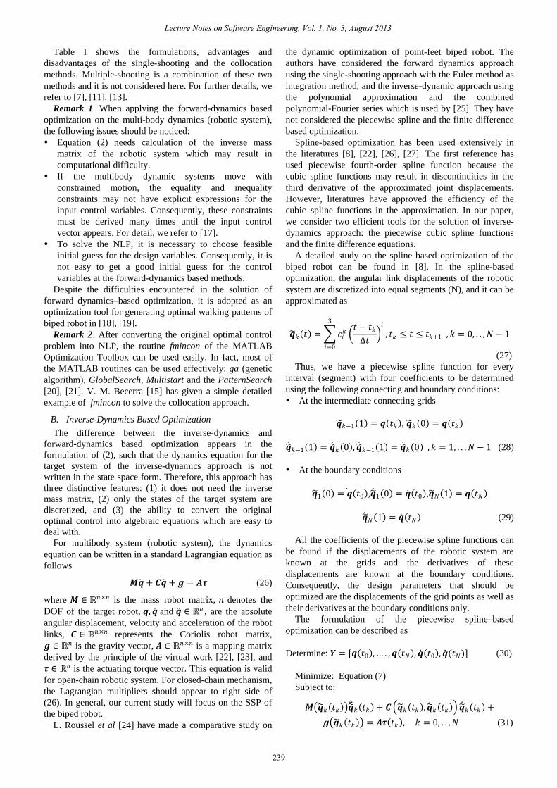
Table I shows the formulations, advantages and

disadvantages of the single-shooting and the collocation

methods. Multiple-shooting is a combination of these two

methods and it is not considered here. For further details, we

refer to [7], [11], [13].

Remark 1. When applying the forward-dynamics based

optimization on the multi-body dynamics (robotic system),

the following issues should be noticed:

Equation (2) needs calculation of the inverse mass

matrix of the robotic system which may result in

computational difficulty.

If the multibody dynamic systems move with

constrained motion, the equality and inequality

constraints may not have explicit expressions for the

input control variables. Consequently, these constraints

must be derived many times until the input control

vector appears. For detail, we refer to [17].

To solve the NLP, it is necessary to choose feasible

initial guess for the design variables. Consequently, it is

not easy to get a good initial guess for the control

variables at the forward-dynamics based methods.

Despite the difficulties encountered in the solution of

forward dynamics–based optimization, it is adopted as an

optimization tool for generating optimal walking patterns of

biped robot in [18], [19].

Remark 2. After converting the original optimal control

problem into NLP, the routine fmincon of the MATLAB

Optimization Toolbox can be used easily. In fact, most of

the MATLAB routines can be used effectively: ga (genetic

algorithm), GlobalSearch, Multistart and the PatternSearch

[20], [21]. V. M. Becerra [15] has given a simple detailed

example of fmincon to solve the collocation approach.

B. Inverse-Dynamics Based Optimization

The difference between the inverse-dynamics and

forward-dynamics based optimization appears in the

formulation of (2), such that the dynamics equation for the

target system of the inverse-dynamics approach is not

written in the state space form. Therefore, this approach has

three distinctive features: (1) it does not need the inverse

mass matrix, (2) only the states of the target system are

discretized, and (3) the ability to convert the original

optimal control into algebraic equations which are easy to

deal with.

For multibody system (robotic system), the dynamics

equation can be written in a standard Lagrangian equation as

follows

𝑴𝒒 + 𝑪𝒒 + 𝒈 = 𝑨𝝉 (26)

where 𝑴 ∈ ℝ𝑛×𝑛 is the mass robot matrix, 𝑛 denotes the

DOF of the target robot, 𝒒,𝒒 and 𝒒 ∈ ℝ𝑛 , are the absolute

angular displacement, velocity and acceleration of the robot

links, 𝑪 ∈ ℝ𝑛×𝑛 represents the Coriolis robot matrix,

𝒈 ∈ ℝ𝑛 is the gravity vector, 𝑨 ∈ ℝ𝑛×𝑛 is a mapping matrix

derived by the principle of the virtual work [22], [23], and

𝝉 ∈ ℝ𝑛 is the actuating torque vector. This equation is valid

for open-chain robotic system. For closed-chain mechanism,

the Lagrangian multipliers should appear to right side of

(26). In general, our current study will focus on the SSP of

the biped robot.

L. Roussel et al [24] have made a comparative study on

the dynamic optimization of point-feet biped robot. The

authors have considered the forward dynamics approach

using the single-shooting approach with the Euler method as

integration method, and the inverse-dynamic approach using

the polynomial approximation and the combined

polynomial-Fourier series which is used by [25]. They have

not considered the piecewise spline and the finite difference

based optimization.

Spline-based optimization has been used extensively in

the literatures [8], [22], [26], [27]. The first reference has

used piecewise fourth-order spline function because the

cubic spline functions may result in discontinuities in the

third derivative of the approximated joint displacements.

However, literatures have approved the efficiency of the

cubic–spline functions in the approximation. In our paper,

we consider two efficient tools for the solution of inverse-

dynamics approach: the piecewise cubic spline functions

and the finite difference equations.

A detailed study on the spline based optimization of the

biped robot can be found in [8]. In the spline-based

optimization, the angular link displacements of the robotic

system are discretized into equal segments (N), and it can be

approximated as

𝒒 𝑘 𝑡 = 𝑐𝑖𝑘

3

𝑖=0

𝑡 − 𝑡𝑘∆𝑡

𝑖

, 𝑡𝑘 ≤ 𝑡 ≤ 𝑡𝑘+1 ,𝑘 = 0, . . ,𝑁 − 1

(27)

Thus, we have a piecewise spline function for every

interval (segment) with four coefficients to be determined

using the following connecting and boundary conditions:

At the intermediate connecting grids

𝒒 𝑘−1 1 = 𝒒 𝑡𝑘 , 𝒒 𝑘 0 = 𝒒 𝑡𝑘

𝒒 𝑘−1 1 = 𝒒 𝑘 0 ,𝒒 𝑘−1 1 = 𝒒 𝑘 0 ,𝑘 = 1, . . ,𝑁 − 1 (28)

At the boundary conditions

𝒒 𝑁 1 = 𝒒 𝑡𝑁 (29)

All the coefficients of the piecewise spline functions can

be found if the displacements of the robotic system are

known at the grids and the derivatives of these

displacements are known at the boundary conditions.

Consequently, the design parameters that should be

optimized are the displacements of the grid points as well as

their derivatives at the boundary conditions only.

The formulation of the piecewise spline–based

optimization can be described as

Determine: 𝒀 = [𝒒 𝑡0 ,… . ,𝒒 𝑡𝑁 ,𝒒 𝑡0 ,𝒒 (𝑡𝑁)] (30)

Minimize: Equation (7)

Subject to:


239

𝒒 1 0 = 𝒒 𝑡0 ,𝒒 1 0 = 𝒒 𝑡0 ,𝒒 𝑁 1 = 𝒒 𝑡𝑁

𝑴 𝒒 𝑘 𝑡𝑘 𝒒 𝑘 𝑡𝑘 + 𝑪 𝒒 𝑘 𝑡𝑘 ,𝒒 𝑘 𝑡𝑘 𝒒 𝑘 𝑡𝑘 +

𝒈 𝒒 𝑘 𝑡𝑘 = 𝑨𝝉 𝑡𝑘 , 𝑘 = 0, . . ,𝑁 (31)

with (13)-(16).

Whereas in the finite difference approach, the velocity

and acceleration of the dynamic system can be

approximated directly using the finite difference approach as

follows.

𝒒 𝑡𝑘 = (𝒒(𝑡𝑘+1) − 𝒒(𝑡𝑘−1)) 2.∆𝑡 , 𝑘 = 0, . . ,𝑁 (32)

𝒒 𝑡𝑘 = (𝒒(𝑡𝑘+1) − 2𝒒(𝑡𝑘) + 𝒒(𝑡𝑘−1)) ∆𝑡2 , 𝑘 = 0, . . ,𝑁

(33)

For detail we refer to [28], [29]. Thus, the formulation of

the finite difference based optimization is as follows:

Determine: Equation (30)

Minimize: Equation (7)

subject to: 𝑴 𝒒 𝑡𝑘 𝒒 𝑡𝑘 + 𝑪 𝒒 𝑡𝑘 ,𝒒 𝑡𝑘 𝒒 𝑡𝑘 +

𝒈 𝒒 𝑡𝑘 = 𝑨𝝉 𝑡𝑘 , 𝑘 = 0, . . ,𝑁 (34)

with (13) to (16).

Remark 3. In effect, we applied the spline-based

optimization and the finite difference approach on a simple

example cited from [6]. The results show that the latter can

be implemented faster and easier than the former. We will

not describe the details here due to the limited space.

III. DYNAMIC OPTIMIZATION OF 6-DOF BIPED ROBOT

Due to the easy use of the finite difference-based

optimization, it was employed to generate optimal motion of

the 6-DOFs biped robot during the single support phase

(SSP) with different cases as we will see in the simulation

section. Fig.2a shows the structure of the investigated biped

robot. The physical parameters are shown in TABLE II.

This section identifies the necessary constraints that can

guarantee natural human motion, as follows:

1) Boundary conditions constraints

Relative displacement of the knee joints and swing

ankle:

5 ≤ 𝑞2(𝑡𝑘) − 𝑞1(𝑡𝑘) ≤ 𝑝𝑖/2, 𝑘 = 0, . . ,𝑁

5 ≤ 𝑞4(𝑡𝑘) − 𝑞5(𝑡𝑘) ≤ 𝑝𝑖/2, 𝑘 = 0, . . ,𝑁

𝑝𝑖/2 ≤ 𝑞6(𝑡𝑘) − 𝑞5(𝑡𝑘) ≤ 3𝑝𝑖/2, 𝑘 = 0, . . ,𝑁 (40)

ZMP-constraint:

In general, there are two concepts used in the literature as

follows:

Concept 1. This is commonly used in the field of biped

robot which states that the location of reaction force is equal

to the ZMP as long as the biped mechanism is stable, as

shown in Fig. 2(b), therefore;

𝑥𝑍𝑀𝑃 𝑡𝑘 = (𝑚6𝑔 𝑑6 − 𝑢1 𝑡𝑘 ) 𝐹𝑦 𝑡𝑘 , 𝑘 = 0, . . ,𝑁

(41)

Thus, the necessary associated constraint is

where 𝑑6 = 𝑂6𝑐6 , 𝑙𝑓1 = 𝑂6𝐴 and 𝑙𝑓1 = 𝑂6𝐵

Fig. 2. The biped robot configuration at the initial single support phase.

TABLE II: THE PHYSICAL PARAMETERS OF THE BIPED ROBOT [30]

𝑖 𝑙𝑖 = 𝑂𝑖𝑂𝑖+1 𝑑𝑖 = 𝑂𝑖𝑐𝑖 𝑚𝑖 𝐼𝑖

1 0.45 0.26 3.61 0.06

2 0.45 0.261 3.69 0.062

3 0.45 0.2 10.3 0.145

4 0.45 0.189 3.66 0.06

5 0.45 0.192 3.53 0.058

6 0.3 0.073 2.05 0.016

In addition, the following constraints of the reaction

forces that should be satisfied


240

Initial configuration of the swing leg:

𝑥𝑠𝐴 𝑡0 + 𝐿𝑠𝑡𝑒𝑝 = 0,𝑥 𝑠𝐴 𝑡0 = 0,𝑦𝑠𝐴 𝑡0 = 0,

𝑦 𝑠𝐴 𝑡0 = 0 (35)

Final configuration of the swing leg:

𝑥𝑠𝐵 𝑡𝑁 − 𝐿𝑠𝑡𝑒𝑝 = 0,𝑥 𝑠𝐵 𝑡𝑁 = 0, 𝑦𝑠𝐵 𝑡𝑁 = 0,

𝑦 𝑠𝐵 𝑡𝑁 = 0 (36)

where all the notations are shown in Fig. 2.

2) Path constraints

Hip motion:

𝑥 𝑕𝑖𝑝 𝑡𝑘 > 0 ,𝑘 = 0, . . ,𝑁 (37)

𝑕𝑚𝑖𝑛 ≤ 𝑦𝑕𝑖𝑝 𝑡𝑘 ≤ 𝑕𝑚𝑎𝑥 ,𝑘 = 0, . . ,𝑁 (38)

Swing foot motion:

0.01 ≤ 𝑦𝑠𝐴 𝑡𝑘 , 𝑘 = 1, . . ,𝑁 − 1

0.01 ≤ 𝑦𝑠𝐵 𝑡𝑘 , 𝑘 = 1, . . ,𝑁 − 1 (39)

𝑢1(𝑡𝑘) + 𝐹𝑦 𝑡𝑘 𝑥𝑍𝑀𝑃(𝑡𝑘) −𝑚6𝑔𝑑6 = 0

−𝑙𝑓2 ≤ 𝑥𝑍𝑀𝑃 𝑡𝑘 ≤ 𝑙𝑓1, 𝑘 = 0, . . ,𝑁 (42)

−𝐹𝑦 𝑡𝑘 < 0 , 𝑘 = 0, . . ,𝑁

−𝐹𝑥 − 𝜇𝐹𝑦 𝑡𝑘 < 0, 𝑘 = 0, . . ,𝑁

𝐹𝑥 − 𝜇𝐹𝑦 𝑡𝑘 < 0, 𝑘 = 0, . . ,𝑁 (43)

Concept 2 [8], [9], [27]. It is assumed that the ground

reaction forces can be equivalently represented by two

normal forces 𝐹𝑦𝐴 ,𝐹𝑦𝐵 applied at end points A and B of the

foot, with a horizontal force acting in the sole, as shown in

Fig. 2 (b). Thus, the conditions that should be satisfied are

−𝐹𝑦𝐴 𝑡𝑘 < 0 , 𝑘 = 0, . . ,𝑁

−𝐹𝑦𝐵 𝑡𝑘 < 0, 𝑘 = 0, . . ,𝑁

−𝐹𝑥 𝑡𝑘 − 𝜇(𝐹𝑦𝐴 𝑡𝑘 + 𝐹𝑦𝐵 𝑡𝑘 ) < 0, 𝑘 = 0, . . ,𝑁

𝐹𝑥 𝑡𝑘 − 𝜇(𝐹𝑦𝐴 𝑡𝑘 + 𝐹𝑦𝐵 𝑡𝑘 ) < 0, 𝑘 = 0, . . ,𝑁 (44)

3) Bounded constraints

𝒒𝑚𝑖𝑛 ≤ 𝒒 𝑡𝑘 ≤ 𝒒𝑚𝑎𝑥 ,𝑘 = 0, . . ,𝑁

𝒒 𝑚𝑖𝑛 ≤ 𝒒 𝑡𝑘 ≤ 𝒒 𝑚𝑎𝑥 ,𝑘 = 0 and 𝑁 (45)

Performance index (objective function)

In general, there are miscellaneous performance indices

that can be used depending on the aim of the designer. If the

minimum energy is required, the literature prefers the

actuating torque cost on the energetic cost due to the

instability problems of the latter. If the designer intends to

focus on the best stability of the biped mechanism, the

minimum deviation of ZMP can be used as cost function [1].

The latter reference has used combined cost function of the

sum of the deviation of ZMP and the minimum energy.

However, it can simply be dealt with ZMP as a constraint

and deals with the minimum energy as cost function.

Anyway, we chose the actuating torques as a cost

function to be minimized.

𝐽 = 𝒖𝑇𝒖𝑡𝑓

𝑡0𝑑𝑡 = 𝒖𝑘

𝑇𝒖𝑘 .∆𝑡𝑁−1𝑘=0 (46)

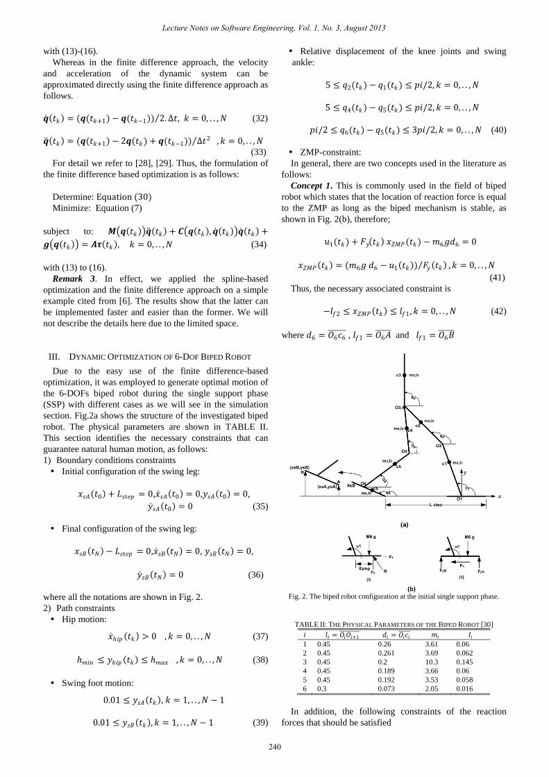
IV. SIMULATION RESULTS AND DISCUSSION

After converting the dynamic optimization into parameter

optimization, any NLP algorithm can be used. Most

literatures [4], [8], [18] have used local solver represented

by fmincon routine for the solution of the parameter

optimization. It should be noted that this command needs

good initial guess to capture feasible local minimum. We

tried to use an arbitrary initial guess, but no feasible solution

can be obtained. However, the inverted–pendulum based

gait can provide us very good initial guess. Therefore, we

depended on this strategy in all investigated cases [31]. One

of the disadvantages of the fmincon is that it can get stuck in

local minimum, therefore, hybrid genetic-sequential

quadratic programming (ga-fmincon) was used to capture

the global minimum, as shown in Fig. 3. However, we got

the same minimum point resulted by the local solver. For

details about the hybrid genetic- SQP we refer to [21], [32]-

[34].

Fig. 3. Flow chart of hybrid genetic–local solver.

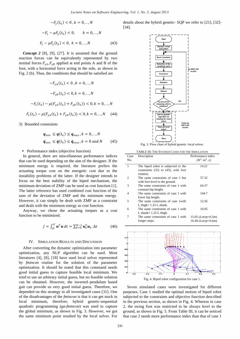
TABLE III: THE STUDIED CASES FOR THE SIMULATION

Case

No.

Description Performance index

(𝑁2 .𝑚2. 𝑠)

1

2

3

4

5

6

7

The biped robot is subjected to the

constraints (35) to (45), with foot

rotation.

The same constraints of case 1 but

with foot level to the ground.

The same constraints of case 1 with

constant hip height.


lower hip height.

The same constraints of case 1with

L thigh= 1.25 L shank.


L shank= 1.25 L thigh.


longer steps.

14.21

57.32

64.37

144.7

12.56

16.05

15.05 (𝐿𝑠𝑡𝑒𝑝=0.5m)

16.49 (𝐿𝑠𝑡𝑒𝑝=0.6m)

Fig. 4. Biped robot configuration for case 1.


241

Seven simulated cases were investigated for different

purposes. Case 1 studied the optimal motion of biped robot

subjected to the constraints and objective function described

in the previous section, as shown in Fig. 4. Whereas in case

2, the swing foot was restricted to be always level to the

ground, as shown in Fig. 5. From Table III, it can be noticed

that case 2 needs more performance index than that of case 1

Fig. 5. Biped robot configuration for case 2.

On the other hand, the effect of the thigh and shank length

were studied via cases 5 and 6 by keeping the total length of

the leg fixed and changing the proportion of the thigh and

the shank. The longer thighs the slightly less energy can be

needed. Whereas, the increase in the required energy is

slight if the shank length is longer than the thigh length. The

last case included the effect of increase of the step length.

The longer steps the slightly more actuating torques are

demanded. The time elapsed in all cased was taken as 0.5 s

while the step length was assumed equal to 0.4 m in cases 1-

6.

V. CONCLUSIONS

This paper focuses on three issues: the selection of the

suitable direct method for suboptimal control of the biped

robot, the suitable algorithm for the solution of the global

minimum of the NLP, and the effect of different constraints

on the required energy of the biped robot. The finite

difference approach can be used efficiently to solve the

suboptimal trajectory of the biped mechanism. While the

genetic-SQP can get the global minimum of the NLP. Lastly,

it can be concluded that more imposed constraints on the

biped robot, more energy is needed. In general, more energy

can be required in the case of

Restriction of the swing foot to be level to the ground.

Reducing the hip height or constraining the hip to move

in constant height.

Longer shanks than thighs.

Longer steps or high step speed.

In effect, a slight increase of the energy was produced in

the last two cases. Despite the easy use of the suboptimal

control problem, it can give approximate solution. Therefore,

further study is necessary to deal with the problem in real

time application.

REFERENCES

[1] P. R. Vundavilli and D. K. Pratihar, ―Gait Planning of Biped Robots

Using Soft Computing: An Attempt to Incorporate Intelligence,‖ in

Intelligent Autonomous Systems: Foundation and Applications, D. K.

Pratihar and L. C. Jain, Ed., Germany: Springer-Verlag, 2010, ch. 4,

pp. 57-85.

[2] H. F. N. Al-Shuka, F. Allmendinger, and B. Corves, Modeling,

stability and walking pattern generators of biped robots: A historical

perspective.

[3] S. Kajita and K. Tani, ―Experimental study of biped dynamic walking

in the linear inverted pendulum mode,‖ in Proc. IEEE Conf. Robotics

and Automation, 1995, vol. 3, pp. 2885-2891.

[4] C. Chevallereau, G. Bessonnet, G. Abba, and Y. Aoustin, Bipedal

Robots, Modeling, Design and Building Walking Robots, 1st ed.,U.K.:

John Wiley and Sons Inc ,2009,ch. 4,pp. 219-265.

[5] R. D. Robinett III, D. G. Wilson, G. R. Eisler, and H. E. Hurtado,

―Applied dynamic programming for optimization of dynamical

systems,‖ SIAM, Philadelphia, USA, 2005.

[6] M. G. Pandy, F. C. Anderson, and D. G. Hull, ―A parameter

optimization approach for the optimal control of large-scale

musculoskeletal,‖ J. Biomech. Eng., vol. 114, no. 4, pp. 450-460,

1992.

[7] M. Diehl, ―Numerical optimal control,‖ Lecture notes, Optimization

in Engineering Center (OPTEC) and Electrical Engineering

Department (ESAT), K. V. Leuven, Belgium, 2011.

[8] P. Seguin and Bessonnet, ―Generating optimal walking cycles using

spline-base state parameterization,‖ International Journal of

Humanoid Robotics, vol. 2, no. 1, pp. 47-80, 2005.

[9] M. Rostami and G. Bessonnet, ―Sagittal gait of a biped robot during

the single support phase. Part 2: Optimal motion,‖ Robotica, vol. 19,

pp. 241-253, 2001.

[10] G. Bessonnet, S. Chesse, and P. Sardain,‖ Generating optimal gait of

a human-sized biped robot,‖ in Proc. the 5th Int. Conf. Climbing and

Walking Robots, Paris, 2002, pp. 241-253.

[11] D. G. Hull, ―Conversion of optimal control problems into parameter

optimization problems,‖ AIAA, Guidance, Navigation and control

performance, San Diego, 1996.

[12] C. J. Goh and K. L. Teo, ―Control parameterization, A unified

approach to optimal problem with general constraints,‖ Automatica,

vol. 24. no. 1, pp. 3-18, 1988.

[13] B. Chachuat, ―Optimal control, Lectures 19-20: Direct solution

methods,‖ Department of chemical engineering, McMaster University,

Canada, 2009.

[14] S. C. Chapra, Applied numerical methods with MATLAB® for

engineers and scientists, New York, USA: McGraw Hill Higher

Education, 2008.

[15] V. M. Becerra, ―Practical direct collocation methods for

computational optimal control,‖ in Modeling and optimization in

space engineering, G. Fasano and J. D. Pinter, Eds., Springer

Optimization and Its Applications, 2013.

[16] O. von Stryk, ―Numerical solution of optimal control problems by

direct collocation,‖ in Optimal control-Calculus of variations, optimal

control theory and numerical methods, R. Bulrisch, A. Miele, J. Stoer,

and K.-H. Well, Eds., International Series of Numerical Mathematics,

pp. 129-143, 1993.

[17] J. T. Betts, ―Practical methods of optimal control using nonlinear

programming,‖ SIAM, Philadelphia, USA, 2001.

[18] C. Azevedo, P. Poignet, and B. Espiau, ―On line optimal control for

biped robot,‖ 15th Teriennial World Congress, Barcelona, Spain, 2002.

[19] L. Roussel, C. Canudas-de-Wit, and A. Goswami, ―Generation of

energy optimal complete gait cycles for bipedal robot,‖ in Proc.

Conference on Robotics and Automation, IEEE, vol. 3, pp. 2036-2041,

1998.

[20] Optimization Toolbox™, User’s Guide, The MathWorks, Inc., 2011.

[21] Global Optimization Toolbox™, User’s Guide, The MathWorks, Inc.,

2011.

[22] A. Hamon and Y. Aoustin, ―Cross four-bar linkage for the knees of a

planar bipedal robot,‖ in Proc. IEEE-RAS International Conference

on Humanoid Robots, 2010, pp.379-384.

[23] S. Tzafestas, M. Raibert, and C. Tzafestas, ―Robust sliding mode

control applied to 5-link biped robot,‖ Journal of Intelligent and

Robotic Systems, vol. 15, pp. 67-133, 1996.

[24] L. Roussel, C. Canudas-de-Wit, and A. Goswami, ―Comparative

study of methods for energy-optimal gait generation for biped robots,‖

International Conference on Informatics and Control, 1997.

[25] V. Yen and M. L. Nagurka, ―Suboptimal trajectory planning of a five-

link human locomotion model,‖ Biomechanics of normal and

prosthetic gait, ASME, BED-vol. 4 and DSC-vol. 7, pp. 17-22, 1987.

[26] C.-S. Lin, P.-R. Chang, and J. Y. S. Luh, ―Formulation and

optimization of cubic polynomial trajectories for industrial robots,‖

IEEE Transactions on automatic control, vol. AC-28, no. 12, pp.

1066-1074, 1983.

[27] T. Saidouni and G. Bessonnet, ―Generating globally optimised

sagittal gait of a biped robot,‖ Robotica, vol. 21, pp. 199-210,2003.

[28] Q. Wang, ―A study of alternative formulations for optimization of

structural and mechanical systems subjected to static and dynamic

loads,‖ PhD Dissertation, University of IOWA, USA, 2006.


242

due to the imposed constraint. For the next cases (case 3-7),

we considered case 1 as reference for the purpose of

comparison. In cases 3 and cases 4, more energy is needed if

the biped robot constrained to move with constant hip or

lower hip height. The more imposed constraints, the more

energy are demanded.

[29] Q. Wang and J. S. Arora, ―Alternative formulations for transient

dynamic response optimization,‖ AIAA, vol. 43, no. 10, pp. 2188-

2195, 2005.

[30] B. Vanderborght, ―Dynamic stabilization of the biped Lucy powered

by actuators with controllable stiffness,‖ PhD dissertation, Vrije

Universiteit Brussel, Belgium, 2007.

[31] H. F. N. Al-Shuka and B. J. Corves, ―On the walking Pattern

generators of biped robot,‖ Journal of Automation and Control

Engineering, vol. 1, no. 2, pp.149-155, 2013.

[32] N. Yokoyama and S. Suzuki, ―Flight trajectory optimization using

genetic algorithm combined with gradient method,‖ ITEM, vol. 1, no.

1, 2001.

[33] F. Yengui, L. Labrak, F. Frantz, R. Daviot, N. Abouchi, and I.

O’Connor, ―Hybrid GA-SQP algorithm for analog circuits sizing,‖

Circuits and Systems, vol. 3, pp. 146-152, 2012.

[34] K. Okuda, K. Yonemoto, and T. Akiyama, ―Hybrid optimal trajectory

generation using genetic algorithm and sequential quadratic

programming,‖ ICROS-SICE International Joint Conference, Japan,

2009.

Hayder F. N. Al-Shuka was born in Baghdad, Iraq in 1979. He received

the B.Sc and M.Sc. degrees from Baghdad and Al-Mustansiriya

Universities respectively, Baghdad, Iraq, in 2003 and 2006 respectively.

Since 2006, he has been assigned as an assistant lecturer in Baghdad

University at the department of Mechanical Engineering. He is currently

PhD student at the RWTH Aachen University at the Department of

Mechanism and Machine Dynamics. His research interests include the

walking patterns and control of biped robots.

Burkhard J. Corves was born in Kiel, Germany in 1960. He received the

Diploma and PhD degrees in Mechanical Engineering from RWTH Aachen

University, Aachen, Germany, in 1984 and 1989 respectively. From 1991

until 2000, he got teaching assignment in RWTH Aachen University. Since

2000, he has been appointed as university professor and director of the

department of Mechanism and Machine Dynamics of RWTH Aachen

University. The research interests of Prof. Dr. Corves include the

kinematics and dynamics of mechanisms and robots.

W.-H. Zhu is an engineering technical officer at the Canadian Space

Agency. His specialty is on precision control of complex robotic systems

characterized by his book entitled Virtual Decomposition Control published

by Springer-Verlag in its STAR series. Dr. Zhu also published 60+ papers

in leading international journals and conference proceedings.


243

on the dynamic optimization of biped robot - lnselnse.org/papers/52-ca021.pdf · ·...

Documents