on the dilution of market power - higher … · on the dilution of market power * sergey kokovin...
TRANSCRIPT

Sergey Kokovin. Mathieu Parenti.
Jacques-François Thisse. Philip Ushchev
ON THE DILUTION
OF MARKET POWER
BASIC RESEARCH PROGRAM
WORKING PAPERS
SERIES: ECONOMICS
WP BRP 176/EC/2017
This Working Paper is an output of a research project implemented at the National Research University Higher
School of Economics (HSE). Any opinions or claims contained in this Working Paper do not necessarily reflect the
views of HSE
On the Dilution of Market Power*
Sergey Kokovin� Mathieu Parenti� Jacques-François Thisse� Philip Ushchev
October 18, 2017
Abstract
We show that a market involving a handful of large-scale �rms and a myriad of small-scale �rms
may give rise to di�erent types of market structure, ranging from monopoly or oligopoly to monopolistic
competition through new types of market structure. In particular, we �nd conditions under which the
free entry and exit of small �rms incentivizes big �rms to sell their varieties at the monopolistically
competitive prices, behaving as if in monopolistic competition. We call this result the dilution of market
power. The structure of preferences is the main driver for a speci�c market structure to emerge as an
equilibrium outcome.
Keywords: dominant �rms, monopolistically competitive fringe, monopolistic competition, oligo-
poly, contestability.
JEL Classi�cation: D43, F12 and L13.
*We gratefully acknowledge comments by D. Spulber, E. Zhelobodko and participants of ESEM and EARIE conferences.The study has been funded by the Russian Academic Excellence Project `5-100' and grant RFBR 16-06-00101.
�Novosibirsk State University and NRU-Higher School of Economics (Russia). Email: [email protected]�ECARES, Université Libre de Bruxelles and CEPR. Email: [email protected]�CORE-UCLouvain (Belgium), NRU-Higher School of Economics (Russia) and CEPR. Email: [email protected]¶NRU-Higher School of Economics (Russia). Email: [email protected]
2
1 Introduction
According to Bruce D. Henderson, the founder of the Boston Consulting Group, �a stable competitive market
never has more than three signi�cant competitors.� Using a sample of more than 160 U.S. industries, two
base-time periods, and numerous performance measures, Uslay et al. (2010) �nd that most industries
consist of three large generalists and numerous small and specialized producers, which succeed if they are
able to operate in a niche market. However controversial the so-called �Rule of Three� may be, it seems
unquestionable that many industries are dominated by a handful of big �rms, which share the market with
many small �rms. Using a sample of 50, 000 U.S. �rms, Hottman et al. (2016) observe that almost 90
percent of sales in a product group are produced by the 10 largest �rms, while 98 percent of �rms have
market shares smaller than 2 percent. Similarly, the empirical trade literature documents the fact that a
handful of �rms account for a considerably large share of exports in many countries (Bernard et al., 2012).
In this paper, we develop a simple, new theory which captures the interactions between big and
small �rms and fully characterizes the market outcome. The key idea is to combine two kinds of �rms: a
discrete number of atomic players, which represent big �rms, and a continuum of nonatomic players, which
represent small �rms. Our setting thus blends oligopolistic and monopolistically competitive �rms, which all
produce di�erent varieties of the same di�erentiated product. Formally, a big �rm supplies a positive mass
of varieties, whereas a small �rm supplies a single variety. Owing to the di�erence in their product scope,
�rms adopt di�erent attitudes toward competition: the big �rms understand that they can strategically
manipulate the market, whereas the small �rms, which are each negligible to the market, treat the market
conditions as given and choose their outputs (or prices) accordingly. Big and small �rms di�er here in kind
because the latter are negligible to the market, while the former are not. This is to be contrasted with
Melitz (2003) where the so-called big and small �rms di�er in types but not in kind because they are all
negligible to the market (Neary, 2010).
In the wake of general-equilibrium models with imperfect competition (Hart, 1985) and the Stackelberg-
Spence-Dixit literature on entry deterrence (Spence, 1977; Dixit, 1979), we assume that big �rms are aware
that their choices a�ect the size of the competitive fringe. More speci�cally, the market process is described
as a two-stage game. At the �rst stage, a big �rm chooses its outputs (or prices), anticipating the reactions
of the small �rms. At the second stage, the small businesses choose their outputs (or prices), treating the
big �rm's choice parametrically. In other words, the small �rms enter or exit the market, whereas the big
�rms always stay in business. The same setting is used in the dominant �rm model where one big �rm
chooses its sale price while anticipating the reactions of a large number of small �rms which treat this price
3
as a given (Markham, 1951). Note, however, the di�erence between this model, where the mass of small
�rms is exogenous, and ours, where it is endogenous. We discuss the staging of the game further in Section
2.
Our main �nding is an e�ect new to the literature, which we christen the dilution of market power.
The essence of this e�ect is that, despite being endowed with the ability to strategically manipulate the
market, a large �rm may �nd it rational to disregard this ability and mimic the behavior of small �rms.1
In other words, the large �rms adopt the same aggressive pricing rule as the one followed by the �rms
belonging to the monopolistically competitive �rms.2 Therefore, the market structure is observationally
equivalent to monopolistic competition.
We illustrate this e�ect by considering an economy where consumers have linear-quadratic preferences,
while the supply side involves one large incumbent and a monopolistically competitive fringe. Whenever
the equilibrium market structure is hybrid, i.e. it involves �rms of both kinds, the dilution of the big �rm's
market power always occurs. But why is this so? Although the incumbent can manipulate the total output
available on the market through its own output, it understands that the mass of small �rms varies so that
the equilibrium aggregate output is the same regardless of its own behavior. In other words, the fringe
acts as a bu�er that stabilizes competition. We will see that a necessary and su�cient condition for this
to happen is that the big �rm is not too big relative to the market. Otherwise, the incumbent chooses to
either deter or blockade entry, as in Dixit (1979).
Next, we show that the dilution of market power keeps its relevance far beyond this simple example.
The key-factor is that the demands faced by �rms are single-aggregate, i.e. all the cross-e�ects in the
demand system are captured by a scalar function whose value plays the role of a market aggregate (Pollak,
1972). This condition is satis�ed for a broad class of demand systems, including those generated by
additive preferences (Zhelobodko et al., 2012), indirectly additive preferences (Bertoletti and Etro, 2017),
and homothetic demand systems with a single aggregator (Matsuyama and Ushchev, 2017). We show that,
when the market involves several big �rms, all �rms are heterogeneous and demands are single-aggregate,
then any hybrid market outcome displays the dilution of market power. This is because the equilibrium
market aggregate pinned down by free entry is independent of the big �rms' choices. As a consequence,
1The dilution of market power has a strong contestability �avor. Indeed, the entry of small �rms, which act non-strategically,su�ces to discipline the big �rm since this one chooses to sell its output as the small �rms do. What is surprising (at least tous) is the fact that adopting such an aggressive behavior is rational on the part of the big �rm. Note, however, the di�erencewith Baumol (1980) and successors. The threat of entry per se is not su�cient here to make the market more competitive. Itis the turnover of small �rms that incentivizes the incumbent to behave as competitively as the small �rms. Another majordi�erence is that the key factor lies in the nature of preferences, rather than in cost considerations.
2By pricing rule we mean here an operator which maps the demand schedule faced by a �rm into the pro�t-maximizingprice as a function of the �rm's marginal cost. Therefore, the same pricing rule does not mean that �rms sell at the sameprice and share the same markups, as the big and small �rms are likely to have di�erent marginal costs.
4
both kinds of �rms treat the market aggregate parametrically, but they do so for very di�erent reasons: the
small �rms are by nature non-strategic, while the big �rms accurately anticipate that the small �rm's best
response is �at in the domain of accommodated entry.
The dilution of market power also has a number of far-reaching implications. One such implication is
the consequences of idiosyncratic technological shocks to large �rms. Speci�cally, if a large �rm is subject
to, say, an exogenous productivity improvement, the equilibrium behavior of the other big �rms remains
the same. Another implication is that neither the emergence of new big �rms nor the merger of a few of
them give rise to major changes economy-wide. All these shocks only a�ect the size of the monopolistically
competitive fringe, without causing any changes in the pro�t-maximizing strategies chosen by the �rms in
the fringe.
In contrast, the dilution of market power does not generally occur when the demand system involves
two or several aggregates, as under quadratic preferences without an outside good (Demidova, 2017) and
under homothetic preferences described by Kimball's (1995) �exible aggregator. In this case, big �rms
behave strategically. However, if we consider the possibility of multiple fringes (which may be interpreted,
e.g., as populations of �rms providing di�erent quality levels), the dilution of market power is restored when
the number of aggregates equals the number of fringes.
In short, our setting allows for an endogenous determination of market structure. Depending on the
market size and the preference for diversity, there is either oligopolistic or monopolistic competition.
Related literature. The foregoing discussion shows that our paper is related to di�erent strands of
literature, including industrial organization, trade theory and general equilibrium under imperfect compe-
tition. In what follows, we discuss the most relevant contributions. It was shown in the 1970s that, when
large traders are similar to each other, or when for each large trader there are small traders similar to it,
the core of an exchange economy coincides with the set of competitive allocations. In other words, the
market power of big traders is diluted (see Gabszewicz and Shitovitz, 1992, for a survey). Our results have
a similar �avor. However, as suggested by Okuno et al. (1980), it is more natural to study such issues in
a non-cooperative setting, which is what we accomplish in this paper. Industrial organization and trade
models with multi-product �rms include Allanson and Montagna (2005), Bernard et al. (2011), Dhingra
(2013), Mayer et al. (2014). Although these authors use di�erent approaches to model multi-product �rms,
they all assume that each �rm is negligible to the market. We di�er from all of them in that multi-product
�rms are able to manipulate the market. By showing that these �rms may choose not to manipulate the
market, we identify conditions for these various models to provide an accurate description of the functioning
5

of markets.
Etro (2006, 2008) models the idea of big and small �rms by assuming that a �rm is big when it is the
leader of a Stackelberg game and a �rm is small when it is a follower. Hence, small �rms are also able to
manipulate the market outcome. Etro (2008) shows that the leaders are more aggressive than the followers
when only big �rms are free to enter the market in the second stage of the game. This di�erence in results
is because, in our setting, the followers pursue the aggressive strategy of pricing at average cost. Therefore,
the leaders cannot adopt a more aggressive behavior than the followers. Neary (2010) suggests a di�erent
approach in which �rms choose to be big or small. Instead, we assume that �rms are born big or small,
but our results show that, under some conditions, the di�erences in kind is immaterial for the equilibrium
outcome. Our paper is more directly linked to Shimomura and Thisse (2012) and Parenti (2017). Even
though the dilution does not hold in their simultaneous game, these authors show that the presence of small
�rms incentivize the big �rms to behave more aggressively than in a purely oligopolistic environment. This
points to the same direction as the dilution of market power.
Even closer to us is the approach developed by Anderson et al. (2015). The great merit of this paper
is to link together results that are a priori disparate. Once oligopolistic �rms have chosen to enter the
market, their pro�ts depend on their own action and an aggregate of all other �rms' actions. Therefore,
each �rm wants to manipulate the market aggregate, so that the dilution of market power never holds.
Rather, we are interested in studying the impact of a monopolistically competitive fringe on the market
outcome. Furthermore, unlike Anderson et al. (2015), we do not impose restrictions on the functional form
of the aggregate, which is given here by any function mapping �rms' strategies into a scalar. Finally, our
analysis is not restricted to the case of a single aggregate. We show that the dilution of market power holds
true when the number of aggregates and fringes is the same. For all these reasons, the two papers are to
be viewed as complements rather than substitutes.
The rest of the paper is organized as follows. The aim of Section 2 is to highlight the e�ect we call the
dilution of market power. To achieve this, we use a simple dominant-�rm-type model with linear-quadratic
preferences, one big �rm and a monopolistically competitive fringe. Section 3 provides a general setting
with single-aggregate preferences, which clari�es how far we can go with this result. Section 4 discusses the
cases of multiple aggregates and multiple fringes. Section 5 concludes.
6
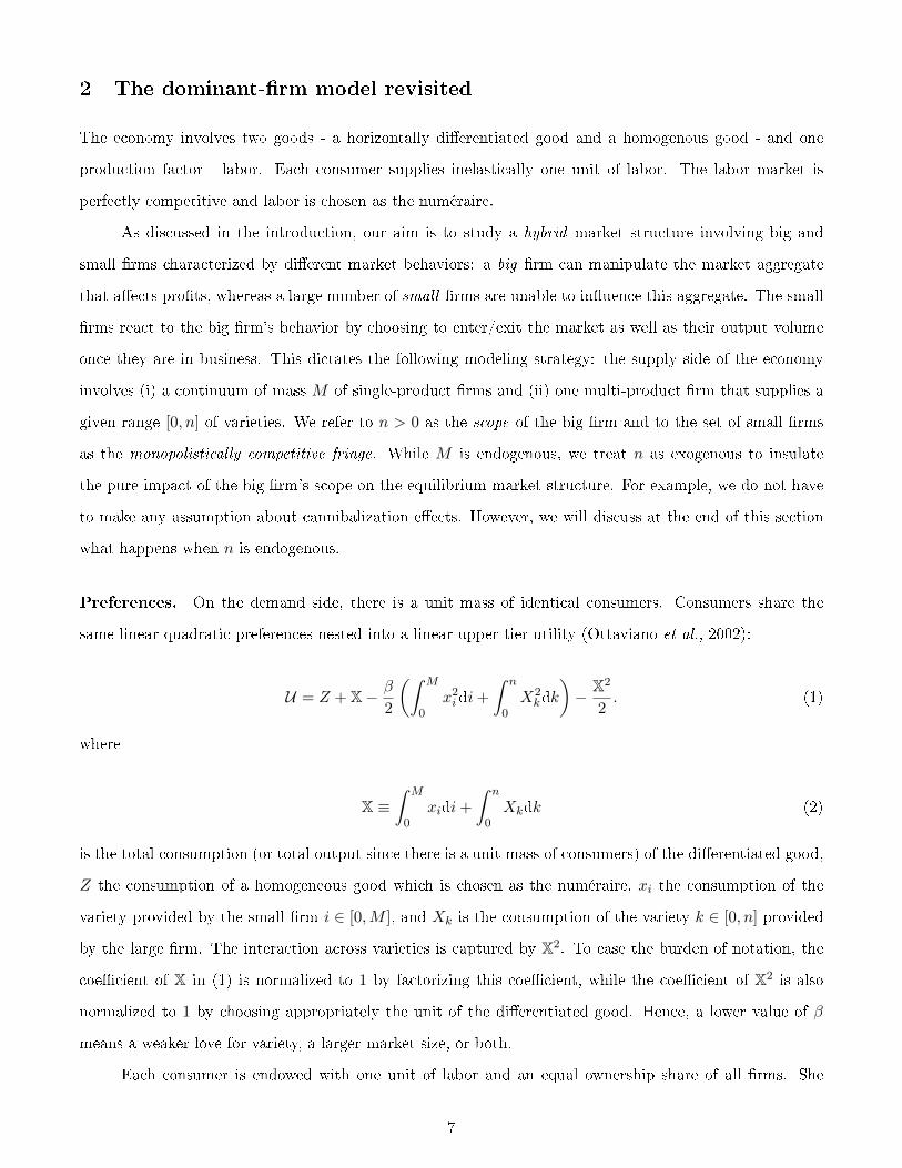
2 The dominant-�rm model revisited
The economy involves two goods - a horizontally di�erentiated good and a homogenous good - and one
production factor - labor. Each consumer supplies inelastically one unit of labor. The labor market is
perfectly competitive and labor is chosen as the numéraire.
As discussed in the introduction, our aim is to study a hybrid market structure involving big and
small �rms characterized by di�erent market behaviors: a big �rm can manipulate the market aggregate
that a�ects pro�ts, whereas a large number of small �rms are unable to in�uence this aggregate. The small
�rms react to the big �rm's behavior by choosing to enter/exit the market as well as their output volume
once they are in business. This dictates the following modeling strategy: the supply side of the economy
involves (i) a continuum of mass M of single-product �rms and (ii) one multi-product �rm that supplies a
given range [0, n] of varieties. We refer to n > 0 as the scope of the big �rm and to the set of small �rms
as the monopolistically competitive fringe. While M is endogenous, we treat n as exogenous to insulate
the pure impact of the big �rm's scope on the equilibrium market structure. For example, we do not have
to make any assumption about cannibalization e�ects. However, we will discuss at the end of this section
what happens when n is endogenous.
Preferences. On the demand side, there is a unit mass of identical consumers. Consumers share the
same linear-quadratic preferences nested into a linear upper-tier utility (Ottaviano et al., 2002):
U = Z + X− β
2
(ˆ M
0x2i di+
ˆ n
0X2kdk
)− X2
2. (1)
where
X ≡ˆ M
0xidi+
ˆ n
0Xkdk (2)
is the total consumption (or total output since there is a unit mass of consumers) of the di�erentiated good,
Z the consumption of a homogeneous good which is chosen as the numéraire, xi the consumption of the
variety provided by the small �rm i ∈ [0,M ], and Xk is the consumption of the variety k ∈ [0, n] provided
by the large �rm. The interaction across varieties is captured by X2. To ease the burden of notation, the
coe�cient of X in (1) is normalized to 1 by factorizing this coe�cient, while the coe�cient of X2 is also
normalized to 1 by choosing appropriately the unit of the di�erentiated good. Hence, a lower value of β
means a weaker love for variety, a larger market size, or both.
Each consumer is endowed with one unit of labor and an equal ownership share of all �rms. She
7

maximizes her utility subject to the budget constraint:
Z +
ˆ M
0pixidi+
ˆ n
0PkXkdk ≤ y,
where pi denotes the price of variety i and Pk the price of variety k, while y > 0 is consumer's income.
Inverse demands and pro�ts. First-order conditions for utility maximization yield the following inverse
demand functions for each variety i ∈ [0,M ] and each variety k ∈ [0, n]:
p(xi,X) = 1− X− βxi, p(Xk,X) = 1− X− βXk. (3)
For simplicity, we assume in this section that all marginal costs to zero and denote by f > 0 a small
�rm's �xed cost. Therefore, �rm i's pro�ts are given by
πi = (1− X− βxi)xi − f.
Note that we have normalized the market size to 1. If the market size were given by L, the �xed cost
f would be replaced with f/L in the analysis developed below. Therefore, a larger market is equivalent to
a lower �xed cost f , which facilitates the entry of small �rms.
The big �rm's pro�ts are given by
N(X) =
ˆ n
0(1− X− βXk)Xkdk,
where X ≡ (Xk)k∈[0,n] is the big �rm's production pro�le.
Since it is negligible to the market, small �rm accurately treats the total output X as a parameter.
By contrast, (2) shows that the big �rm expects its action to a�ect the value of X through its total output
Xmp de�ned as follows:
Xmp ≡ˆ n
0Xkdk. (4)
The timing of the game is as follows. The incumbent moves �rst and the monopolistically competitive
�rms second. Besides the reasons discussed in the introduction, this staging may be justi�ed on the following
grounds. First, the di�erence in entry behavior �ts a fairly robust empirical fact, i.e. the survival probability
of a �rm is positively correlated with its size. Second, the above staging captures the idea that the big
�rm is committed to the market due to the large investment this �rm has to make to build its production
8

capacity. By contrast, the assumption of free entry and exit re�ects the high turnover characterizing small
�rms in many industries, probably because these �rms invest little money to be in business. We seek a
subgame perfect Nash equilibrium and solve the game by backward induction.
2.1 Stage 2: The small �rms' equilibrium strategies
Assume that a hybrid market structure prevails in equilibrium. In this case, a small �rm observes the choice
made by the big �rm through the total output Xmp and chooses its pro�t-maximizing output. This yields
the equilibrium output, price and pro�ts as a function of X:
x∗(X) =1− X
2β, p∗(X) =
1− X2
, π∗(X) =1
4β(1− X)2 − f.
It is readily veri�ed that the zero-pro�t condition π∗(X) = 0 implies that equilibrium total output is
a constant equal to
X∗ = XD ≡ 1− 2√βf < 1. (5)
For XD > 0, we assume that β < 1/(4f); otherwise, the small �rms never enter because f is too high.
In this case, the equilibrium total output is independent of the big �rm's behavior: it depends only upon
the parameter β, which captures the intensity of preference for diversity, and the small �rms' �xed cost f ,
which determines the easiness of entry into the fringe. Note also that X∗ is independent of the scope n of
the big �rm.
Substituting X∗ into x∗(X) and p∗(X), we determine the small �rm's equilibrium output and its
equilibrium price:
x∗ =
√f
β> 0, p∗ =
√βf > 0. (6)
Therefore, small �rms' equilibrium price and output are independent of the big �rm's choice, which
implies that the big �rm in�uences the monopolistically competitive fringe through the mass of small �rms
only. In addition, the zero-pro�t condition implies that the small �rms price their varieties at their average
cost: p∗ = f/x∗.
Evaluating (2) at a symmetric outcome yields X = Xmp +Mx. Solving for M , we obtain the equili-
brium mass of small �rms conditional upon Xmp:
M∗(Xmp) = (1− Xmp)
√f
β− 2f. (7)
9

This expression shows that the fringe acts as a bu�er that stabilizes the total output at the value X∗
through a change in the equilibrium mass of small �rms. When the big �rm increases (decreases) its total
output Xmp, the size of the fringe shrinks (expands).
Observe that Xmp = XD is the unique solution to the equation M∗(Xmp) = 0. Therefore, the
monopolistically competitive fringe disappears when Xmp is su�ciently large:
Xmp ≥ XD,
which implies that XD is the big �rm's minimal total output that deters the entry of small �rms. As a
result, we have:
X∗(Xmp) = max {Xmp,XD} . (8)
As shown by Figure 1, the behavior of the big �rm a�ects the equilibrium value of the market
aggregate if and only if Xmp exceeds XD. Otherwise, the big �rm behaves as if it had no market power.
Indeed, this �rm �nds it rational to forego manipulating the equilibrium value of the market aggregate X
by changing its total output Xmp.
Insert Figure 1 about here
Thus, although the big �rm is non-negligible to the market, things work as if it were so. As a
consequence, any hybrid outcome in which the equilibrium level X∗mp of the big �rm's output is such that
X∗mp < XD, is observationally equivalent to a purely monopolistically competitive equilibrium obtained by
replacing the big �rm with a mass n of small �rms. We call this e�ect dilution of market power and discuss
it in more detail in sub-section 2.4.
2.2 Stage 1: The large �rm's equilibrium strategy
The big �rm chooses its output anticipating the small �rms' optimal responses. As a result, the big �rm
treats X∗ as a given. Thus, the big �rm's adjusted inverse demand for each its variety k, with or without
a monopolistically competitive fringe, is de�ned by the following expression:
p(Xk,X∗) = 1− X∗(Xmp)− βXk. (9)
Combining (9) with (8), the big �rm's pro�t function N(X) may be written as follows:
10
N(X) = min
{Xmp − β
ˆ n
0X2kdk − X2
mp, (1− XD)Xmp − βˆ n
0X2kdk
}. (10)
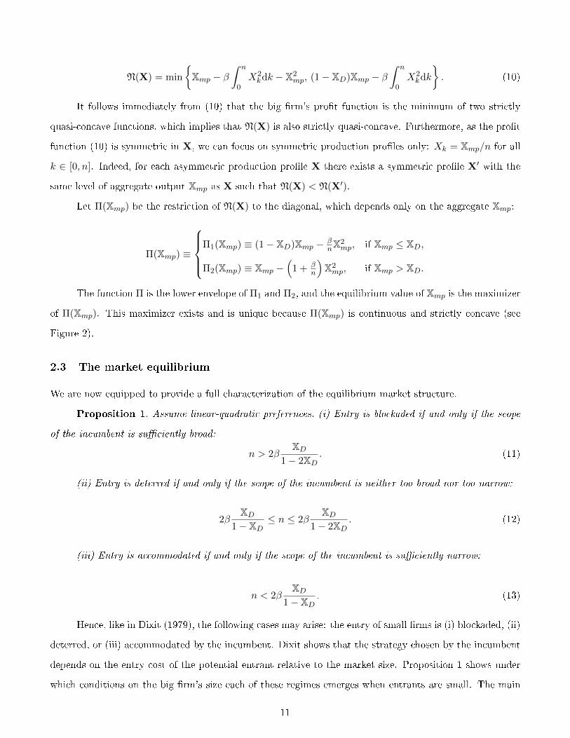
It follows immediately from (10) that the big �rm's pro�t function is the minimum of two strictly
quasi-concave functions, which implies that N(X) is also strictly quasi-concave. Furthermore, as the pro�t
function (10) is symmetric in X, we can focus on symmetric production pro�les only: Xk = Xmp/n for all
k ∈ [0, n]. Indeed, for each asymmetric production pro�le X there exists a symmetric pro�le X′ with the
same level of aggregate output Xmp as X such that N(X) < N(X′).
Let Π(Xmp) be the restriction of N(X) to the diagonal, which depends only on the aggregate Xmp:
Π(Xmp) ≡
Π1(Xmp) ≡ (1− XD)Xmp − β
nX2mp, if Xmp ≤ XD,
Π2(Xmp) ≡ Xmp −(
1 + βn
)X2mp, if Xmp > XD.
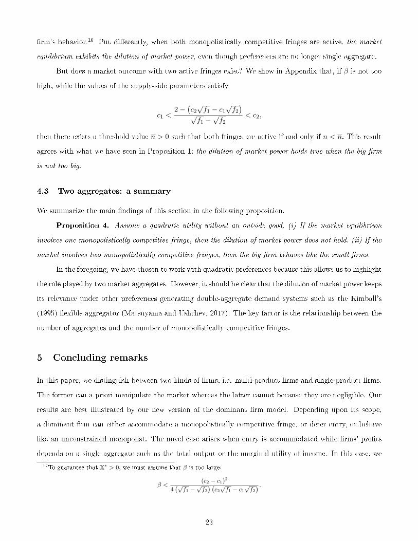
The function Π is the lower envelope of Π1 and Π2, and the equilibrium value of Xmp is the maximizer
of Π(Xmp). This maximizer exists and is unique because Π(Xmp) is continuous and strictly concave (see
Figure 2).
2.3 The market equilibrium
We are now equipped to provide a full characterization of the equilibrium market structure.
Proposition 1. Assume linear-quadratic preferences. (i) Entry is blockaded if and only if the scope
of the incumbent is su�ciently broad:
n > 2βXD
1− 2XD. (11)
(ii) Entry is deterred if and only if the scope of the incumbent is neither too broad nor too narrow:
2βXD
1− XD≤ n ≤ 2β
XD1− 2XD
. (12)
(iii) Entry is accommodated if and only if the scope of the incumbent is su�ciently narrow:
n < 2βXD
1− XD. (13)
Hence, like in Dixit (1979), the following cases may arise: the entry of small �rms is (i) blockaded, (ii)
deterred, or (iii) accommodated by the incumbent. Dixit shows that the strategy chosen by the incumbent
depends on the entry cost of the potential entrant relative to the market size. Proposition 1 shows under
which conditions on the big �rm's size each of these regimes emerges when entrants are small. The main
11

distinctive feature of our approach lies in the endogenous entry and exit of small �rms, a di�erence that
has unsuspected (at least to us) implications.
The proof of Proposition 1 goes as follows. Observe that Π(Xmp) is the lower envelope of two
concave parabolas, while Π1(Xmp) and Π2(Xmp) satisfy the following properties: (i) Π1(0) = Π2(0) = 0, (ii)
Π1(XD) = Π2(XD) = XD − (1 + β/n)X2D, and (iii) Π′1(XD) > Π′2(XD). As illustrated by Figure 2, three
cases may arise.
Insert Figure 2 about here
Blockaded entry. Assume that Π′1(XD) > Π′2(XD) > 0 (see Figure 2a). Since Π1(Xmp) and Π2(Xmp)
are both increasing in the neighborhood of XD, the maximizer of Π(Xmp) exceeds XD, which implies that
the big �rm is an unconstrained monopolist. It is readily veri�ed that Π′2(XD) > 0 holds if and only if the
incumbent �rm's scope is given by (11).
Since Π2(Xmp) is strictly concave, the big �rm's pro�t-maximizing output and pro�ts are obtained
from the �rst-order-condition:
X∗mp(n) =n
2(β + n), Π∗(n) =
n
4(β + n).
In short, if the incumbent is large enough, entry is su�ciently costly, or both, then the monopolist
may accurately ignore the potential entry of small �rms. Otherwise, entry can never be blockaded because
the market size is too large for the big �rm to ignore the small �rms. In this case, does the incumbent deter
or accommodate entry?
Entry deterrence. Assume now that Π′1(XD) > 0 > Π′2(XD) (see Figure 2b). In this case, the maximizer
X∗mp of Π(Xmp) is exactly the kink XD. Indeed, the incumbent chooses an output preventing the entry of
small �rms if and only if X∗mp ≥ XD, which is equivalent to M∗(X∗mp) = 0. The inequalities Π′1(XD) > 0 >
Π′2(XD) hold if and only if the breadth of the big �rm's scope is given by (12).
Since XD is the smallest value of X that deters entry, it has the nature of a �limit output�, which is
the quantity counterpart of limit pricing. Under entry deterrence, the incumbent's total output and pro�ts
are equal to
X∗mp(n) = XD, Π∗(n) = XD[1−
(1 +
β
n
)XD].
12

Accommodating entry. Last, assume that Π′2(XD) < Π′1(XD) < 0 (see Figure 2c). Since Π1(Xmp)
and Π2(Xmp) are both decre0asing in Xmp in the neighborhood of XD, so does Π(Xmp). Therefore, the
maximizer of Π(Xmp) is smaller than XD. This occurs if and only if the big �rm's scope n is small enough
relative to the market size and given by (13). Maximizing Π1(Xmp) with respect to Xmp yields:
X∗mp(n) =n
2β(1− XD) = n
√f
β, Π∗(n) =
n
4β(1− XD)2 = nf.
To sum up, as n steadily decreases, the incumbent's pro�ts and markups (weakly) decrease, thus
implying that the big �rm's market power fades away. During this process, the market outcome displays
a gradual transition from pure monopoly to monopolistic competition through entry deterrence. Note that
the same holds when the market size steadily rises while n remains constant. Since accommodated entry
leads to new and unsuspected results, we focus below on the case of hybrid markets.
2.4 The dilution of market power
When entry is accommodated, the incumbent faces an inverse demand for variety k that accounts for the
massM∗(Xmp) of small �rms that enter the market in the second stage. Although the incumbent is a priori
able to manipulate X through Xmp, it anticipates that the mass (7) of small �rms will adjust in a way such
that the equilibrium value of X is always equal to X∗ regardless of the value taken by Xmp. In other words,
the incumbent accurately treats X∗ as a parameter.
Plugging (5) into (9), it is straightforward to show that the pro�t-maximizing output and price of
variety k under accommodating entry are given by
X∗ =
√f
β, P ∗ ≡
√βf,
which are the same as those given by (6), that is, the equilibrium output and price of a small �rm. Therefore,
the big �rm's equilibrium total output is X∗mp = nx∗, while its equilibrium pro�ts are Π∗(n) = nf .
Stated di�erently, when the large �rm accommodates the presence of small �rms, the former chooses
to sell the quantity x∗ given by (6) for each of its varieties, which it prices at the same level as the
varieties sold by the latter. In other words, if the incumbent is not �too� big relative to the market, there is
monopolistic competition. In other words, the big �rm's market power is dissolved in an ocean of small �rms.
This amounts to saying that the incumbent behaves like a multidivisional �rm in which autonomous �pro�t
centers� produce each a speci�c variety and maximize their own pro�ts, while ignoring demand linkages
13

within the �rm's product range. While the divisionalization of a �rm is often justi�ed by the desire to
prevent pyramiding management costs, our model provides a justi�cation driven by the demand side only.
This shows that a �rm able to manipulate the market may �nd it pro�t-maximizing to disregard
its strategic power, an e�ect which we christen the dilution of market power. The above example and the
analysis developed in the next section show that the dilution of market power owns nothing to the cost
side; it is fully driven by the structure of the demand size. Note also that the empirical evidence suggests
that the small �rms may be signi�cant in number, while their market share is very small. However, the size
of the monopolistically competitive fringe is immaterial for the dilution of market power to hold. What
matters is the existence of entry and exit �ows in the fringe.
2.5 Endogenizing the big �rm's product range
So far, we have assumed that the size n of the product range was given. In line with Spulber (1981), we
assume that the established �rm chooses its scope n before its output. At the stage 0 of the game, the big
�rm's pro�t function is as follows:
Π∗(n) =
n
4(β+n) if n > 2β XD1−2XD
,
XD[1−
(1 + β
n
)XD]
if 2β XD1−XD
≤ n ≤ 2β XD1−2XD
,
fn if n < 2β XD1−XD
,
which can be shown to be strictly increasing, concave and once continuously di�erentiable (see Figure 3 for
an illustration).
Insert Figure 3 here
Building on the spatial model of �exible manufacturing (Eaton and Schmitt, 1994) and following
Mayer et al. (2014) who use linear-quadratic preferences, we assume that the big �rm has a baseline variety
at k = 0, which corresponds to its core competency. To supply another variety, the �rm must incur an
additional cost that increases with the �distance� to its baseline variety. For simplicity, we assume that
the development cost of variety k is given by c(k) = tk with t > 0. When the big �rm's scope is n, the
total cost is therefore equal to tn2. However, our results remain qualitatively the same for more general
speci�cations of the development cost c(k).3
Maximizing Π∗(n)− tn2 with respect to n and using Proposition 1 yields the following result.
3Our conclusions are una�ected when we account for scope economies by assuming that total costs are given by F + tn2
where F > 0 is the cost of launching a R&D division.
14

Proposition 2. Assume core competencies with c(k) = tk. (i) Entry is blockaded if and only if:
t <(1− 2XD)3
8β2XD.
(ii) Entry is deterred if and only if:
(1− 2XD)3
8β2XD≤ t ≤ f
4β
1− XDXD
.
(iii) Entry is accommodated if and only if:
t >f
4β
1− XDXD
. (14)
Hence, we get the following intuitive conditions: the big �rm accommodates entry, hence the dilution
of market power holds, when moving away from core competency is costly, the market is large, and/or the
preference for diversity is strong. In the remaining sections, we will focus on the regime of accommodated
entry.
3 The dilution of market power under single-aggregate preferences
It is tempting to argue that the dilution of market power is an artefact of linear-quadratic preferences. In
this section, we show that this property survives under a much more general condition, i.e. �rms' inverse
demand depends only on the �rm's output and a scalar that aggregates the decisions made by all �rms
(Pollak, 1972). Consider N ≥ 1 big �rms, with �rm j = 1, .., N supplying each a mass nj > 0 of varieties
and producing at marginal cost Cj > 0. We discuss below the case where large �rms can freely enter the
market.
The small �rms are heterogeneous in the sense of Melitz (2003). Prior to entry the small �rms face
uncertainty about their marginal cost but know the continuous distribution Γ(c) from which the marginal
cost c is drawn. To enter the market, the small �rms must bear a sunk cost fe. After entry, each �rm
observes its marginal cost c. In addition, an active c-type �rm must incur a �xed production cost f , so
that producing the quantity xc involves a cost equal to f + cxc.
Consider preferences such that �rms face single-aggregate inverse demands p(·,Λ) where Λ is a scalar
market aggregate which accounts for all the cross-e�ects within the demand system (examples are given
15

below).4 In this case, �rms' pro�t functions may be written as follows:
Πj =
ˆ nj
0[p(Xjk,Λ)− Cj ]Xjkdk, j = 1, ..., N, (15)
π(c) = [p(xc,Λ)− c]xc − f, c ∈ [0, c̄], (16)
where c̄ is the cuto� cost.5
Assumption SA. The inverse demands are single-aggregate and given by p(·,Λ) where the value of
Λ is una�ected by the action of a single small �rm. These demands are such that �rms' pro�ts (15) and
(16) are continuous, strictly quasi-concave in their own strategy for all admissible Λ, and strictly monotone
in the aggregate Λ for all admissible Xjk and xc.6
The strict quasi-concavity assumption is made for the best reply to be a well-de�ned function. That
πc strictly decreases (increases) with Λ means that the market aggregate Λ is a substitute (complement) of
xc.
Assumption SA is satis�ed by the linear demand system (3) where Λ = X. Other examples of demand
systems that are widely used in industrial organization and international trade are given below.
1. Additive preferences. Consider the inverse demands derived from additive preferences (e.g. the
CES and CARA):
U = Me
ˆ c
0u(xc)dΓ(c) +
N∑j=1
ˆ nj
0Uj(Xjk)dk,
where u and Uj are strictly increasing and concave, with u(0) = Uj(0) = 0, whileMe is the mass of entrants.
Denoting by λ the Lagrange multiplier of the budget constraint, the utility-maximizing conditions yield the
following inverse demand functions:
Pjk(Xjk, λ) =U ′j(Xjk)
λ, p(xc, λ) =
u′(xi)
λ.
In this case, the market aggregate, which is the marginal utility of income, is pinned down by the
budget constraint:
Λ ≡ λ = Me
ˆ c
0xcu′(xc)dΓ(c) +
N∑j=1
ˆ nj
0XkU
′j(Xjk)dk.
4Pollak (1972) shows that Marshallian demands are single-aggregate if and only if the inverse demands satisfy the sameproperty.
5To avoid complex issues raised by income endogeneity which stems from redistribution of pro�ts, we assume that �rmsare owned by absentee shareholders. Therefore, since labor is the numéraire, we have y = 1.
6Unlike Acemoglu and Jensen (2013) and Anderson et al. (2015), we do not assume the aggregator Λ to be additivelyseparable in �rms' strategies.
16

Clearly, Λ is una�ected by a change in xc or in Xjk.7
2. Homothetic demand systems with a single aggregator. Another example is given by the
homothetic demand systems with a single aggregator (HSA) studied by Matsuyama and Ushchev (2017).
The HSA inverse demands are given by
p(xc,Λ) =1
Λφ(xc
Λ
), p(Xjk,Λ) =
1
ΛΦj
(Xjk
Λ
), (17)
where φ(·) and Φj(·) are decreasing functions whose elasticities do not exceed one in absolute value. The
market aggregate Λ is implicitly de�ned by the solution to the following �xed-point condition:
Λ = Me
ˆ c
0xcφ
(xcΛ
)dΓ(c) +
N∑j=1
ˆ nj
0XjkΦj
(Xjk
Λ
)dk,
which stems from combining (17) with the budget constraint.
The class of HSA preferences includes both the CES and the translog. The former is obtained by
choosing power functions with the same exponent for φ(·) and Φj(·). The latter is a special case of (17)
where φ(·) and Φj(·) are such that
φ−1(z) =1− γ ln z
z, Φ−1
j (z) =1− γj ln z
z,
where γ and γj , j = 1, ..., N , are positive parameters.
3. Indirectly additive preferences. A further example of single-aggregate demand systems may be
obtained from indirectly additive preferences, that is, the indirect utility is as follows (recall that y = 1):
V = Me
ˆ c
0v (pc) dΓ(c) +
N∑j=1
ˆ nj
0Vj (Pjk) dk,
where v(·) and Vj(·) are decreasing, convex, and twice di�erentiable. The corresponding inverse demand
system is given by
pc =(v′)−1
(Λxc), Pjk =(V ′j)−1
(ΛXjk),
where the market aggregate Λ is given by the solution to the budget constraint:
7Since Λ is the only variable that accounts for income, the properties derived below hold true when the individual incomeis made endogeneous through the redistribution of the big �rms' pro�ts.
17

Me
ˆ c
0xc(v′)−1
(Λxc)dΓ(c) +
N∑j=1
ˆ nj
0Xjk
(V ′j)−1
(ΛXjk)dk = 1.
In sum, the Assumption SA is satis�ed for a broad class of preferences.
Consider the second stage of the sequential game in which the big �rms move �rst and the small
ones second. Being negligible to the market, each small �rm accurately treats the market aggregate Λ as
a parameter and determines its best reply function x∗(Λ). This function is well de�ned under Assumption
SA. This assumption and the envelope theorem imply that the optimal pro�t function π∗c (Λ) is monotone
in Λ. Therefore, for any given Λ, the cuto� condition
π∗c (Λ) ≡ πc(x∗c(Λ),Λ) = 0.
has at most one solution c̄(Λ), which is also monotone in Λ. More speci�cally, c̄(Λ) increases (decreases)
with Λ if and only if π∗c (Λ) increases (decreases) with Λ. Hence, the zero-pro�t condition
ˆ c̄(Λ)
0π∗c (Λ)dΓ(c)− fe = 0 (18)
has a unique solution Λ∗. In other words, as long as entry is accommodated, the equilibrium value Λ∗ of
the market aggregate is uniquely determined and independent of the actions chosen by the big �rms.
In the �rst stage of the game, the big �rms anticipate the equilibrium value Λ∗. Hence, each big �rm
j chooses the quantity X∗jk of its variety k that maximizes its pro�ts [p(Xjk,Λ∗)− Cj ]Xjk, which depend
only upon Xjk.
Consequently, we have the following proposition.
Proposition 3. Assume a hybrid market structure with big and small �rms. Under Assumption SA,
the big �rms behave like the small �rms.
This result has several important implications.
Being non-strategic is a rational strategy. A hybrid market functions �as if� all �rms were to operate
under monopolistic competition. Stated di�erently, the small �rms incentivize the big �rms to refrain from
reducing their output, which renders these �rms more aggressive. Furthermore, since the big and small
�rms are heterogeneous, they do not sell at the same prices. However, under Assumption SA, they adopt
the same pricing rule. In short, Proposition 2 shows that the dilution of market power holds true for a
much broader class of preferences than the linear-quadratic utility.
18
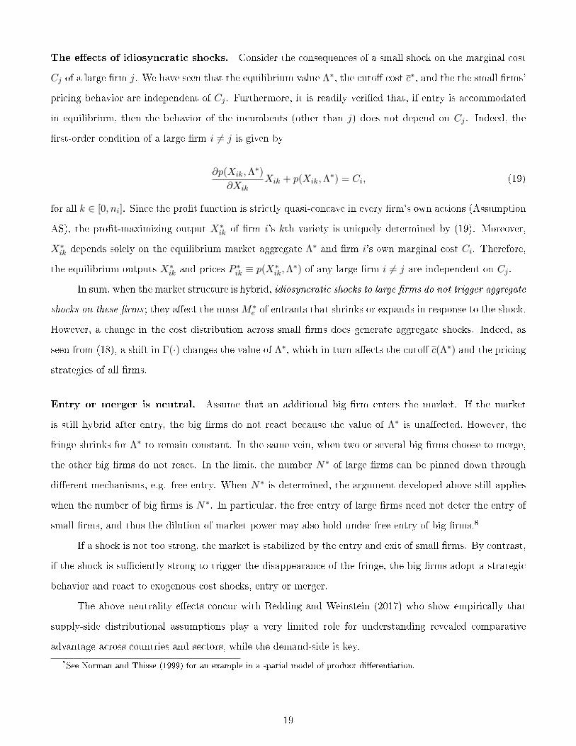
The e�ects of idiosyncratic shocks. Consider the consequences of a small shock on the marginal cost
Cj of a large �rm j. We have seen that the equilibrium value Λ∗, the cuto� cost c∗, and the the small �rms'
pricing behavior are independent of Cj . Furthermore, it is readily veri�ed that, if entry is accommodated
in equilibrium, then the behavior of the incumbents (other than j) does not depend on Cj . Indeed, the
�rst-order condition of a large �rm i 6= j is given by
∂p(Xik,Λ∗)
∂XikXik + p(Xik,Λ
∗) = Ci, (19)
for all k ∈ [0, ni]. Since the pro�t function is strictly quasi-concave in every �rm's own actions (Assumption
AS), the pro�t-maximizing output X∗ik of �rm i's kth variety is uniquely determined by (19). Moreover,
X∗ik depends solely on the equilibrium market aggregate Λ∗ and �rm i's own marginal cost Ci. Therefore,
the equilibrium outputs X∗ik and prices P ∗ik ≡ p(X∗ik,Λ∗) of any large �rm i 6= j are independent on Cj .
In sum, when the market structure is hybrid, idiosyncratic shocks to large �rms do not trigger aggregate
shocks on these �rms; they a�ect the massM∗e of entrants that shrinks or expands in response to the shock.
However, a change in the cost distribution across small �rms does generate aggregate shocks. Indeed, as
seen from (18), a shift in Γ(·) changes the value of Λ∗, which in turn a�ects the cuto� c(Λ∗) and the pricing
strategies of all �rms.
Entry or merger is neutral. Assume that an additional big �rm enters the market. If the market
is still hybrid after entry, the big �rms do not react because the value of Λ∗ is una�ected. However, the
fringe shrinks for Λ∗ to remain constant. In the same vein, when two or several big �rms choose to merge,
the other big �rms do not react. In the limit, the number N∗ of large �rms can be pinned down through
di�erent mechanisms, e.g. free entry. When N∗ is determined, the argument developed above still applies
when the number of big �rms is N∗. In particular, the free entry of large �rms need not deter the entry of
small �rms, and thus the dilution of market power may also hold under free entry of big �rms.8
If a shock is not too strong, the market is stabilized by the entry and exit of small �rms. By contrast,
if the shock is su�ciently strong to trigger the disappearance of the fringe, the big �rms adopt a strategic
behavior and react to exogenous cost shocks, entry or merger.
The above neutrality e�ects concur with Redding and Weinstein (2017) who show empirically that
supply-side distributional assumptions play a very limited role for understanding revealed comparative
advantage across countries and sectors, while the demand-side is key.
8See Norman and Thisse (1999) for an example in a spatial model of product di�erentiation.
19
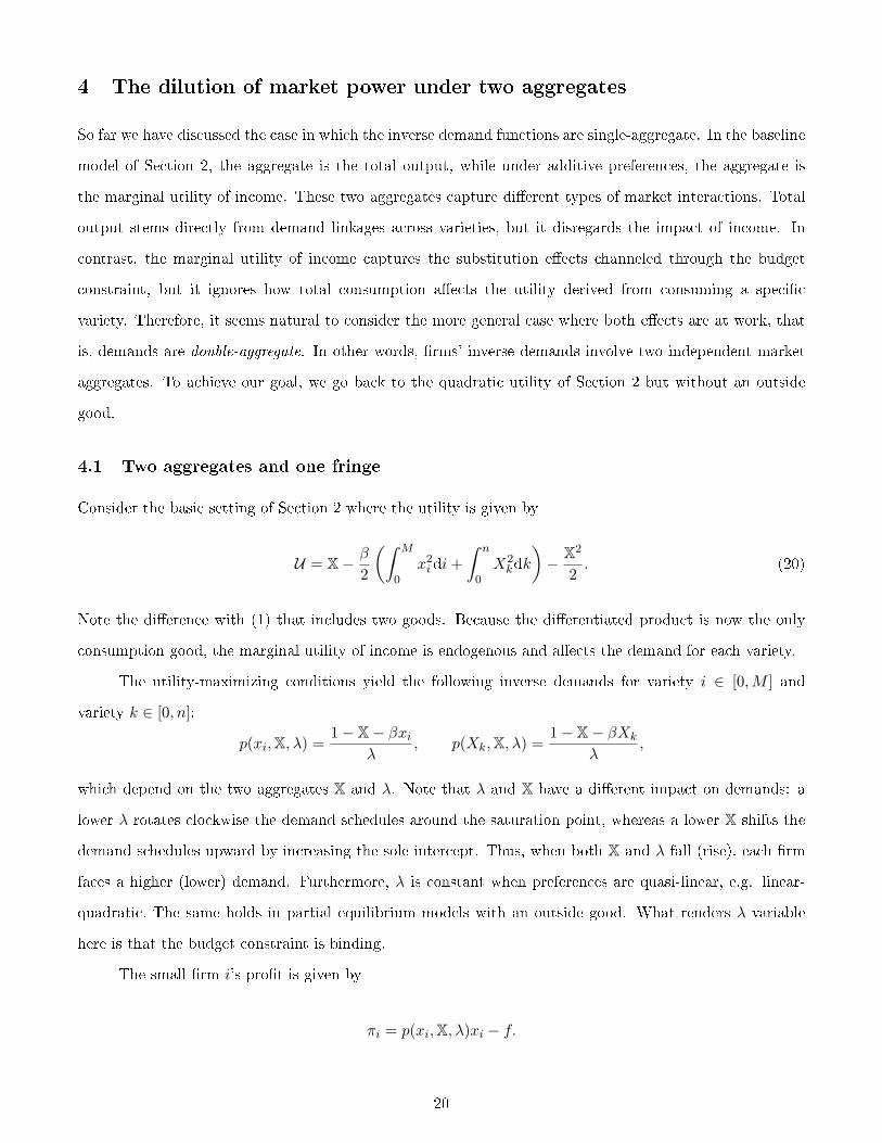
4 The dilution of market power under two aggregates
So far we have discussed the case in which the inverse demand functions are single-aggregate. In the baseline
model of Section 2, the aggregate is the total output, while under additive preferences, the aggregate is
the marginal utility of income. These two aggregates capture di�erent types of market interactions. Total
output stems directly from demand linkages across varieties, but it disregards the impact of income. In
contrast, the marginal utility of income captures the substitution e�ects channeled through the budget
constraint, but it ignores how total consumption a�ects the utility derived from consuming a speci�c
variety. Therefore, it seems natural to consider the more general case where both e�ects are at work, that
is, demands are double-aggregate. In other words, �rms' inverse demands involve two independent market
aggregates. To achieve our goal, we go back to the quadratic utility of Section 2 but without an outside
good.
4.1 Two aggregates and one fringe
Consider the basic setting of Section 2 where the utility is given by
U = X− β
2
(ˆ M
0x2i di+
ˆ n
0X2kdk
)− X2
2. (20)
Note the di�erence with (1) that includes two goods. Because the di�erentiated product is now the only
consumption good, the marginal utility of income is endogenous and a�ects the demand for each variety.
The utility-maximizing conditions yield the following inverse demands for variety i ∈ [0,M ] and
variety k ∈ [0, n]:
p(xi,X, λ) =1− X− βxi
λ, p(Xk,X, λ) =
1− X− βXk
λ,
which depend on the two aggregates X and λ. Note that λ and X have a di�erent impact on demands: a
lower λ rotates clockwise the demand schedules around the saturation point, whereas a lower X shifts the
demand schedules upward by increasing the sole intercept. Thus, when both X and λ fall (rise), each �rm
faces a higher (lower) demand. Furthermore, λ is constant when preferences are quasi-linear, e.g. linear-
quadratic. The same holds in partial equilibrium models with an outside good. What renders λ variable
here is that the budget constraint is binding.
The small �rm i's pro�t is given by
πi = p(xi,X, λ)xi − f.
20

Since the small �rms treat the aggregates X and λ parametrically, their pro�t functions are strictly
concave in xi. Of course, any equilibrium of the fringe features symmetry among small �rms: xi = x all
i ∈ [0,M ].
In the second stage, the large �rm's total output Xmp de�ned by (4) is treated parametrically by the
small �rms. A small �rm's �rst-order condition yields:
x∗(X) =1− X
2β, p∗(X) =
1− X2λ∗(X)
, (21)
where λ∗(X) is pinned down by the zero-pro�t condition:
λ∗(X) =(1− X)2
4βf. (22)
This expression shows that the equilibrium value of the aggregate λ varies with the aggregate X:
the marginal utility of income decreases as the total consumption rises. Therefore, we must know X to
determine λ.
Since marginal costs are zero, the labor market balance implies that the equilibrium mass of entrants
is given by M∗ = 1/f > 0. Combining this with X = Xmp +M∗x∗(X) and (21), we �nd that the impact of
the big �rm on the market aggregate is described as follows:
X∗(Xmp) =
1
1+2βf + 2βf1+2βfXmp, Xmp ≤ 1,
Xmp, Xmp > 1.
(23)
Figure 4 provides an illustration. Comparing Figures 1 and 4 shows why the big �rm now a�ects
the equilibrium value of X: there is no �at spot in Figure 4. As a result, the equilibrium of the second
stage depends on the choice Xmp made by the big �rm in the �rst stage. To put it di�erently, the large
�rm always exploits its strategic power to manipulate the market outcome. This is to be contrasted with
Proposition 1 where X∗ is independent of Xmp when n is not too large.
Insert Figure 4 about here
In the foregoing analysis, we implicitly assume that the monopolistically competitive fringe exists
(x∗ > 0), which holds if and only if Xmp < 1. Combining equation (23) with (21) and (22) yields the
second-stage equilibrium: x∗(Xmp), p∗(Xmp) and λ∗(Xmp). By studying the �rst stage, it is possible to
determine the condition on the size n of the big �rm for this inequality to be satis�ed.
21

4.2 Two aggregates and two fringes
We now assume there are two monopolistically competitive fringes to capture the idea that the two fringes
supply varieties having di�erent qualities, as in Fajgelbaum et al. (2011). In our setting, this can be
reformulated by assuming that �rms in fringe 1 produce at a lower marginal cost but bear a higher �xed
cost than �rms belonging to fringe 2: c1 < c2 and f1 > f2.
Preferences are still given by (20), while the inverse demands for the small �rms are now de�ned by
p(xs,i,X, λ) =1− X− βxs,i
λ,
where s is the fringe index, s = 1, 2. Therefore, we have:
X ≡ˆ M1
0x1,idi+
ˆ M2
0x2,idi+ Xmp, (24)
where Xmp is again the large �rm's total output de�ned by (4).
A small �rm in fringe s maximizes its pro�ts:9
πs(xs) =
(1− X− βxs
λ− cs
)xs − fs, s = 1, 2.
The pro�t-maximizing outputs and prices of small �rms are given, respectively, by
x∗s(X, λ) =1− X− λcs
2β, π∗s(X, λ) =
(1− X− λcs)2
4βλ− fs, s = 1, 2. (25)
Combining π∗s(X, λ) with the free entry conditions π∗1 = π∗2 = 0, we �nd that the equilibrium values
λ∗ and X∗ must satisfy the following relationships:
c1 + 2
√f1β
λ=
1− Xλ
= c2 + 2
√f2β
λ. (26)
Since c1 < c2 and f1 > f2, the equation c1 +2√f1β/λ = c2 +2
√f2β/λ has a unique positive solution
λ∗, while X∗ is pinned down by plugging λ∗ into (26):
λ∗ = 4β
(√f1 −
√f2
c2 − c1
)2
, X∗ = 1− 4β
(√f1 −
√f2
) (c2√f1 − c1
√f2
)(c2 − c1)2
. (27)
As implied by (27), the equilibrium values λ∗ and X∗ of the two aggregates are independent of the big9In what follows, we disregard the variety index i because of symmetry.
22
�rm's behavior.10 Put di�erently, when both monopolistically competitive fringes are active, the market
equilibrium exhibits the dilution of market power, even though preferences are no longer single aggregate.
But does a market outcome with two active fringes exist? We show in Appendix that, if β is not too
high, while the values of the supply-side parameters satisfy
c1 <2−
(c2√f1 − c1
√f2
)√f1 −
√f2
< c2,
then there exists a threshold value n > 0 such that both fringes are active if and only if n < n. This result
agrees with what we have seen in Proposition 1: the dilution of market power holds true when the big �rm
is not too big.
4.3 Two aggregates: a summary
We summarize the main �ndings of this section in the following proposition.
Proposition 4. Assume a quadratic utility without an outside good. (i) If the market equilibrium
involves one monopolistically competitive fringe, then the dilution of market power does not hold. (ii) If the
market involves two monopolistically competitive fringes, then the big �rm behaves like the small �rms.
In the foregoing, we have chosen to work with quadratic preferences because this allows us to highlight
the role played by two market aggregates. However, it should be clear that the dilution of market power keeps
its relevance under other preferences generating double-aggregate demand systems such as the Kimball's
(1995) �exible aggregator (Matsuyama and Ushchev, 2017). The key factor is the relationship between the
number of aggregates and the number of monopolistically competitive fringes.
5 Concluding remarks
In this paper, we distinguish between two kinds of �rms, i.e. multi-product �rms and single-product �rms.
The former can a priori manipulate the market whereas the latter cannot because they are negligible. Our
results are best illustrated by our new version of the dominant �rm model. Depending upon its scope,
a dominant �rm can either accommodate a monopolistically competitive fringe, or deter entry, or behave
like an unconstrained monopolist. The novel case arises when entry is accommodated while �rms' pro�ts
depends on a single aggregate such as the total output or the marginal utility of income. In this case, we
10To guarantee that X∗ > 0, we must assume that β is too large:
β <(c2 − c1)2
4(√f1 −
√f2) (c2√f1 − c1
√f2) .
23

have shown that this aggregate is determined by the sole entry and exit of small �rms. Therefore, even
when the dominant �rm has a relatively large market share, this �rm �nds it pro�t-maximizing to disregard
its ability to manipulate the market, practicing instead a �divisionalization strategy� akin to monopolistic
competition. More generally, we have seen that the presence of a monopolistically competitive fringe may
vastly a�ect the behavior of large �rms in that the former disciplines the latter.
Our results suggest that consumers' preferences, more than producers' costs, determine the market
structure, implying that the on-going emphasis put on cost heterogeneity could well be exaggerated. This
is also in line with the recent empirical �ndings of Hottman et al. (2016) and Redding and Weinstein
(2017). In short, our framework allows the market structure to be endogenized by determining conditions
for oligopolistic competition, monopolistic competition, or hybrid forms of competition to emerge as an
equilibrium outcome.
References
[1] Acemoglu, D., Jensen, M.K. 2013. Aggregate comparative statics. Games and Economic Behavior 81:
27 � 49.
[2] Allanson, P., Montagna, C. 2005. Multiproduct �rms and market structure: An explorative application
to the product life cycle. International Journal of Industrial Organization 23: 587 � 97.
[3] Anderson, S.P., Erkal, N., Piccinin, D. 2015. Aggregative oligopoly games with entry. University of
Virginia, memo.
[4] Baumol, W.J. 1980. Contestable markets: An uprising in the theory of industry structure. American
Economic Review 70: 1 � 15.
[5] Bernard, A.B., Jensen, J.B., Redding, S.J., Schott, P.K. 2012. The empirics of �rm heterogeneity and
international trade. Annual Review of Economics 4: 283 � 313.
[6] Bernard, A.B., Redding, S.J., Schott, P.K. 2011. Multi-product �rms and trade liberalization.Quarterly
Journal of Economics 126: 1271 � 318.
[7] Bertoletti, P., Etro, F. 2017. Monopolistic competition when income matters. Economic Journal 127:
1217 � 43.
[8] d'Aspremont, C., Dos Santos Ferreira, R. Gérard-Varet, L.-A. 1996. On the Dixit-Stiglitz model of
monopolistic competition. American Economic Review 86: 623 � 9.
24

[9] Demidova, S. 2017. Trade policies, �rm heterogeneity, and variable markups. Journal of International
Economics 108: 260 � 73.
[10] Dhingra, S. 2013. Trading away wide brands for cheap brands. American Economic Review 103: 2554
� 84.
[11] Dixit, A.K. 1979. A model of duopoly suggesting a theory of entry barriers. Bell Journal of Economics
10: 20 � 32.
[12] Dixit, A.K., Stiglitz, J.E. 1977. Monopolistic competition and optimum product diversity. American
Economic Review 67: 297 � 308.
[13] Eaton, B.C., Schmitt, N. 1994. Flexible manufacturing and market structure. American Economic
Review 84: 875 � 88.
[14] Eckel, C., Neary, J.P. 2010. Multi-product �rms and �exible manufacturing in the global economy.
Review of Economic Studies 77: 188 � 217.
[15] Etro, F. 2006. Aggressive leaders. RAND Journal of Economics 37: 146 � 54.
[16] Etro, F. 2008. Stackelberg competition with endogenous entry. Economic Journal 118: 1670 � 97.
[17] Fajgelbaum, P., Grossman, G.M., Helpman, E. 2011. Income distribution, product quality, and inter-
national trade. Journal of Political Economy 119: 721 � 65.
[18] Gabszewicz, J.J., Shitovitz, B. 1992. The core in imperfectly competitive economies. In: R. Aumann
and S. Hart (eds.), Handbook of Game Theory with Economic Applications. Volume 1. Amsterdam:
North-Holland, 459 � 83.
[19] Hart, O. 1985. Imperfect competition in general equilibrium: An overview of recent work. In K. Arrow
and S. Honkapohja (eds.), Frontiers in Economics. Oxford: Basil Blackwell, 100 � 49.
[20] Hottman, C., Redding, S.J., Weinstein, D.E. 2016. Quantifying the sources of �rm heterogeneity.
Quarterly Journal of Economics 131: 1291 � 364.
[21] Kimball, M. 1995. The quantitative analytics of the basic neomonetarist model. Journal of Money,
Credit and Banking 27: 1241 � 77.
[22] Markham, J.W. 1951. The nature and signi�cance of price leadership. American Economic Review 41:
891 � 905.
25

[23] Matsuyama, K., Ushchev, P. 2017. Beyond CES: Three alternative classes of �exible homothetic de-
mand systems. CEPR Discussion Paper N◦ 12210.
[24] Mayer, T., Melitz, M., Ottaviano, G.I.P. 2014. Market size, competition, and the product mix of
exporters. American Economic Review 104: 495 � 536.
[25] Melitz, M. 2003. The impact of trade on intraindustry reallocations and aggregate industry producti-
vity. Econometrica 71: 1695 � 725.
[26] Neary, J.P. 2010. Two and a half theories of trade. The World Economy 33: 1 � 19.
[27] Norman, G., Thisse, J.-F. 1999. Technology choice and market structure: Strategic aspects of �exible
manufacturing, Journal of Industrial Economics 47: 345 � 72.
[28] Okuno, M., Postlewaite, A., Roberts, J. 1980. Oligopoly and competition in large markets. American
Economic Review 70: 22 � 31.
[29] Ottaviano, G.I.P., Tabuchi, T., Thisse, J.-F. 2002. Agglomeration and trade revisited. International
Economic Review 43: 409 � 36.
[30] Parenti, M. 2017. International trade with David and Goliath. Journal of International Economics,
forthcoming.
[31] Pollak, R. A. 1972. Generalized separability. Econometrica 40: 431 � 53.
[32] Redding, S.J., Weinstein, D.E. 2017. Accounting for micro and macro patterns of trade. Columbia
University, memo.
[33] Shimomura, K.-I., Thisse, J.-F. 2012. Competition among the big and the small. RAND Journal of
Economics 43: 329 � 47.
[34] Spence, A.M. 1977. Entry, capacity, investment and oligopolistic pricing. Bell Journal of Economics
8: 534 � 44.
[35] Spulber, D.F. 1981. Capacity, output, and sequential entry. American Economic Review 71: 503 � 14.
[36] Uslay, C., Altintig, Z. Ayca, Winsor, R.D. 2010. An empirical examination of the �Rule of Three�:
Strategy implications for top management, marketers, and investors. Journal of Marketing 74: 20 �
39.
26

[37] Zhelobodko, E., Kokovin, S., Parenti, M., Thisse, J.-F. 2012. Monopolistic competition in general
equilibrium: Beyond the constant elasticity of substitution. Econometrica 80: 2765 � 84.
Appendix
We know that
M1x∗1 +M2x
∗2 = X∗ − nX∗, (A.1)
while the budget constraint implies
M1p∗1x∗1 +M2p
∗2x∗2 = 1. (A.2)
As p∗s and x∗s, s = 1, 2, are pinned down by plugging (27) into (25), (A.1) � (A.2) is a system of two
linear equations with two unknowns: M1 and M2.
Lemma 1. The system (A.1) � (A.2) has a unique solution.
Proof. Because c1 < c2, and because the pass-through under linear demands equals 1/2, we have:
p∗2 − p∗1 =c2 − c1
2> 0. (A.3)
�
Hence, the determinant of the system (A.1) � (A.2) is always strictly positive:
β(c2 − c1)x∗1x∗2 > 0.
Hence, the coe�cient matrix is non-degenerate. Q.E.D.
For both fringes to be active, (A.1) � (A.2) must have a positive solution.
Lemma 2. The system (A.1) � (A.2) has a positive solution if and only if the following inequalities
hold :
n
2β + n+
2β
2β + n
1
p∗2< X∗ <
n
2β + n+
2β
2β + n
1
p∗1. (A.4)
Proof. Observe that the slopes of the (A.1)- and (A.2)-loci in the (M1,M2)-plane are equal, respecti-
vely, to x∗1/x∗2 and to p∗1x
∗1/p∗2x∗2. Combining this with p∗2 > p∗1, which is implied by (A.3), we �nd that the
(A.1)-locus is steeper than the (A.2)-locus. Hence, the system (A.1) � (A.2) has a positive solution if and
only if (i) the intercept of the (A.1)-locus with the M2-axis is higher than that of the (A.2)-locus, and (ii)
the intercept of the (A.2)-locus with the M1-axis is further to the right than that of the (A.1)-locus. It is
27

readily veri�ed that (i) and (ii) are equivalent to (A.4). Q.E.D.
We are now equipped to prove that the dilution of market power occurs when the big �rm is not too
big.
Proposition A. Assume that the following inequalities hold :
c1 <2−
(c2√f1 − c1
√f2
)√f1 −
√f2
< c2. (A.5)
Then, β > 0 and n > 0 exist such that both fringes are active if and only if β < β and n < n.
Proof. The inequalities (A.4) can be rewritten as follows:
K1 < n+ 2β < K2, (A.6)
where K1 and K2 are constants de�ned by
Ks ≡(c2 − c1)2
2(√f1 −
√f2
) (c2√f1 − c1
√f2
) [1− 2
cs(√f1 −
√f2
)+ c2√f1 − c1
√f2
]
for s = 1, 2. Furthermore, it is readily veri�ed that (A.5) is equivalent to K1 < 0 < K2. Thus, it remains
to show that n+ 2β < K2 for the proposition hold. Set
β ≡ K2
2=
(c2 − c1)2
4(√f1 −
√f2
) (c2√f1 − c1
√f2
) [1− 2
c2
(√f1 −
√f2
)+ c2√f1 − c1
√f2
],
and assume β ≤ β. Setting n ≡ K2/2β and using (A.6) completes the proof. Q.E.D.
28

29
30

31
Contact details:
Philip Ushchev
National Research University Higher School of Economics (Moscow, Russia).
Center for Market Studies and Spatial Economics, leading research fellow.
E-mail: [email protected]
Any opinions or claims contained in this Working Paper do not necessarily re�ect the
views of HSE.
© Kokovin, Parenti, Thisse, Ushchev, 2017
32