Solar Energy 144 (2017) 40–48

Contents lists available at ScienceDirect

Solar Energy

journal homepage: www.elsevier .com/locate /solener

On the determination of atmospheric longwave irradiance under all-skyconditions

http://dx.doi.org/10.1016/j.solener.2017.01.0060038-092X/� 2017 Elsevier Ltd. All rights reserved.

⇑ Corresponding author.E-mail address: ccoimbra@ucsd.edu (C.F.M. Coimbra).

Mengying Li, Yuanjie Jiang, Carlos F.M. Coimbra ⇑Department of Mechanical and Aerospace Engineering, Jacobs School of Engineering, Center of Excellence in Renewable Resource Integration and Center for Energy Research,University of California in San Diego, 9500 Gilman Drive, La Jolla, CA 92093, USA

a r t i c l e i n f o a b s t r a c t

Article history:Received 23 June 2016Received in revised form 24 December 2016Accepted 3 January 2017

Keywords:Effective sky emissivityEffective sky temperatureDownward longwave irradianceParametric modeling

In this work we review and recalibrate existing models, and present a novel comprehensive model forestimation of the downward atmospheric longwave (LW) radiation for clear and cloudy sky conditions.LW radiation is an essential component of thermal balances in the atmosphere, playing also a substantialrole in the design and operation of solar power plants. Unlike solar irradiance, LW irradiance is not mea-sured routinely by meteorological or solar irradiance sensor networks. In most cases, it must be calcu-lated indirectly from meteorological variables using simple parametric models. Under clear skies,fifteen parametric models for calculating LW irradiance are compared and recalibrated. All modelsachieve higher accuracy after grid search recalibration, and we show that many of the previously pro-posed LWmodels collapse into only a few different families of models. A recalibrated Brunt-family modelis recommended for future use due to its simplicity and high accuracy (rRMSE = 4.37%). To account for thedifference in nighttime and daytime clear-sky emissivities, nighttime and daytime Brunt-type models areproposed. Under all sky conditions, the information of clouds is represented by cloud cover fraction (CF)or cloud modification factor (CMF, available only during daytime). Three parametric models proposed inthe bibliography are compared and calibrated, and a newmodel is proposed to account for the alternationof vertical atmosphere profile by clouds. The proposed all-sky model has 3.8–31.8% lower RMSEs than theother three recalibrated models. If GHI irradiance measurements are available, using CMF as a parameteryields 7.5% lower RMSEs than using CF. For different applications that require LW information duringdaytime and/or nighttime, coefficients of the proposed models are corrected for diurnal and nocturnaluse.

� 2017 Elsevier Ltd. All rights reserved.

1. Introduction

The downward atmospheric longwave irradiance flux (LW, W/m2)is an essential component of radiative balance for solar powerplants and is of great importance in meteorological and climaticstudies, including the forecast of nocturnal temperature variationand cloudiness. It also plays a critical role in the design of radiantcooling systems, as well as in the modeling of weather and climatevariability (Alados et al., 2012; Carmona et al., 2014), and on thedetermination of selective optical properties for photovoltaic pan-els, photovoltaic-thermal collectors, solar thermoelectricity para-bolic disks, etc. (Eicker and Dalibard, 2011; Zaversky et al., 2013).

The downward longwave atmospheric irradiance can be mea-sured directly by pyrgeometers. However, pyrgeometers are notstandard irradiance equipment in most weather stations because

pyrgeometers are relatively expensive and require extensive cali-bration and adjustments to exclude the LW radiation emitted bysurrounding obstacles, buildings and vegetation. Spectral (line-by-line) calculations considering the interactions of LW irradiancewith atmospheric molecules (such as H2O, CO2 and O3), aerosolsand clouds yield reasonable estimates of LW for global calculations,but line-by-line calculations are generally too complex for meteo-rological or engineering use.

A simple approach to estimate LW relies on parametric model-ing of meteorological variables measured routinely at the surfacelevel, such as screening level air temperature and relative humid-ity. The parametric models imply specific assumptions regardingthe vertical structure of the atmosphere (Brunt, 1932; Brutsaert,1975; Ruckstuhl et al., 1984; Maghrabi and Clay, 2011). Theseassumptions are either explicit (Brutsaert, 1975), or implicitlyincluded in the parametric models by locally fitting coefficients(Berdahl and Fromberg, 1982; Tang et al., 2004; Ruckstuhl et al.,

M. Li et al. / Solar Energy 144 (2017) 40–48 41

1984; Bilbao and De Miguel, 2007; Maghrabi and Clay, 2011;Carmona et al., 2014).

In this work we review a large number of previous models fordetermining the downward atmospheric longwave (LW) radiationat the ground level, and propose a novel model for all sky condi-tions (diurnal and nocturnal, clear or cloudy skies). Section 2 out-lines some of the background concepts needed to interpret thedataset and clear sky models used in this work, which aredescribed in Section 3 and in Appendix A. Section 4 discussesand re-calibrates previously proposed models for clear sky condi-tions, and selects the most accurate model family to be used as abasis for the development of an all-sky condition model, which isevaluated against independent data sets. Conclusions from thiswork are presented in Section 6.

2. Background

For longwave atmospheric irradiance (4–100 lm), the back-ground atmosphere can be considered as a gray body, and theLW irradiance is approximated as a fraction of a fictional blackbodyemissive power evaluated at the surface level air temperature(Mills and Coimbra, 2015). This fraction is called the effective skyemissivity esky and is expressed as,

esky ¼ LWrT4

a

ð1Þ

where r ¼ 5:6697� 10�8 W/m2 K4 is the Stefan-Boltzmann con-stant (Mills and Coimbra, 2015) and Ta (K) is the air temperatureat the surface level. This balance can be used to define an effectivesky temperature Tsky (K) by approximating the sky as a blackbody,

LW ¼ rT4sky ð2Þ

Compare Eqs. (1) and (2), the relationship between Tsky and esky is,

Tsky ¼ e1=4skyTa ð3ÞSince esky ranges from 0 to 1, the effective sky temperature is

lower than the surface level air temperature (Mills and Coimbra,2015).

In the parametric modeling, the clear-sky effective emissivity ofthe atmosphere can be expressed as a function of screening levelair temperature Ta (K), relative humidity / (%) and/or other mete-orological variables, including screening level partial pressure ofwater vapor Pw (Pa), dew point temperature Td (K) and moisturecontent d (g/(kg dry air)),

esky;c ¼ f ðTa;/; Pw; Td; dÞ ð4ÞThe partial pressure of water vapor Pw (Pa) and dew point temper-ature Td (K) can be expressed as a function of Ta and / by the Magusexpressions (Alduchov and Eskridge, 1996),

Pw ¼ 610:94/

100

� �exp

17:625ðTa � 273:15ÞTa � 30:11

� �ð5Þ

Td ¼ 243:04 lnðPw=610:94Þ17:625� lnðPw=610:94Þ þ 273:15: ð6Þ

And the moisture content d (kg/(kg dry air)) can be expressed as,

d ¼ Pw

Pa � Pw

Ra

Rw¼ 0:622Pw

Pa � Pw: ð7Þ

where Pa is the air pressure (Pa). In Section 4 of this work, fifteendifferent forms of Eq. (4) are compared and calibrated using mea-surements from seven stations across the contiguous United States,and the most accurate formula is proposed.

The presence of clouds substantially modifies the LW becausethe radiation emitted by water vapor and other gases in the loweratmosphere is supplemented by the emission from clouds. There-fore, under cloudy conditions, the effective sky emissivity is highercompared to clear-sky value. Parametric models can also be usedto estimate all-sky condition LW with the consideration of cloudcontribution,

LW ¼ f ðLWc;CF;CMFÞ ð8Þwhere LWc (W/m2) is the corresponding clear-sky LW, CF (%) is thecloud cover fraction in the sky dome and CMF is a cloud modifica-tion factor,

CMF ¼ 1� GHIGHIc

ð9Þ

where GHI (W/m2) is the global horizontal solar radiation and GHIc(W/m2) is the clear-sky GHI. Note that CMF only has values duringthe daytime. In Section 5, three different forms of Eq. (8) are com-pared and calibrated, and a new model is proposed to achievehigher accuracy.

Therefore, we propose and validate a new parametric modelingof LW for clear- and all-sky conditions applicable to both daytimeand nighttime. We validate the model with data from seven sta-tions over the contiguous United States, for which cloud cover frac-tion data is available in nearby weather stations. A detaileddescription of the dataset is presented in Section 3.

3. Preparation of dataset

3.1. Observational data

The comparison and calibration of parametric models in Sec-tions 4 and 5 are performed and validated using the radiationand meteorological measurements from the SURFRAD (SurfaceRadiation Budget Network) and ASOS (Automated Surface Observ-ing System) operated by NOAA (National Oceanic and AtmosphericAdministration). Currently seven SURFRAD stations are operatingin climatologically diverse regions over the contiguous UnitedStates as shown in Fig. 1 (National Oceanic and AtmosphericAdministration, 2015). Our fitting and validation datasets includemeasurements of year 2012 and year 2013 that are collected inall seven stations. Data from years 2014 and 2015 are not selectedto avoid the influence of El Ni~no and La Ni~na years (Golden GateWeather Service, 2016).

The seven stations, Bondville (in Illinois), Boulder (in Colorado),Desert Rock (in Nevada), Fort Peck (in Montana), Goodwin Creek(in Mississippi), Penn State University (in Pennsylvania) and SiouxFalls (in South Dakota) represent the climatological diversities, asshown in Table 1. Fort Peck and Sioux Falls have a cold and humidclimate with annual averaged temperature and relative humidityaround 7.0 �C and 70%. Bondville and Penn State are cool andhumid with annual averaged temperature around 11.0 �C and rel-ative humidity around 71%. Boulder has a mild climate with annualaveraged temperature and relative humidity of 12.2 �C and 44.7%.Goodwin Creek is warm and humid with annual averaged temper-ature of 16.8 �C and relative humidity of 71.9%. Desert Rock has ahot and dry climate with annual averaged temperature and relativehumidity of 18.8 �C and 27.5%. The seven sites also covers a largealtitude span that ranges from 98 m to 1689 m.

The utilized SURFRAD measurements include 1-min averageddownwelling thermal infrared (IR, W/m2), direct normal solar radi-ation (DNI, W/m2), global horizontal solar radiation (GHI, W/m2),screen level air temperature (Ta, K) and relative humidity of theair (/, %). The Eppley Precision Infrared Radiometer (PIR) measuresthe downwelling IR from the atmosphere. The spectral range of the

Fig. 1. Locations of the 7 SURFRAD stations used in this work (National Oceanic and Atmospheric Administration, 2015).

Table 1Annual average values, 25th and 75th percentile of air temperature (Ta), relative humidity (/), downward atmospheric infrared irradiance (IR) of SURFRAD stations during year2012–2013.

SURFRAD Stations

Parameters Bondville Boulder Desert Rock Fort Peck Goodwin Creek Penn State Sioux Falls

Latitude (�) 40.05 40.13 36.62 48.31 34.25 40.72 43.73Longtitude (�) �88.37 �105.24 �116.02 �105.10 �89.87 �77.93 �96.62Altitude (m) 213 1689 1007 634 98 376 437Data Sampling Rate (minute) 1 1 1 1 1 1 1Average Ta (�C) 11.8 12.2 18.8 5.9 16.8 10.7 8.325th Percentile of Ta (�C) 2.2 4.3 10.6 �3.8 10.0 2.1 �1.875th Percentile of Ta (�C) 20.9 20.6 27.1 16.5 23.9 18.9 19.1Average / (%) 70.7 44.7 27.5 68.2 71.9 71.0 72.125th Percentile of / (%) 58.2 26.2 13.4 52.1 56.8 57.6 58.975th Percentile of / (%) 85.6 61.2 35.5 86.4 89.9 87.4 87.9Average IR (W/m2) 320.7 290.4 308.0 288.9 349.7 318.0 302.425th Percentile of IR (W/m2) 275.1 248.8 268.6 246.7 307.9 276.4 255.875th Percentile of IR (W/m2) 370.6 331.0 342.7 331.9 396.2 366.6 354.0

Closest ASOS stations

Champaign Boulder Desert Rock Wolf Point INTL Oxford State College Sioux Falls

Latitude (�) 40.04 40.04 36.62 48.09 34.38 40.85 43.58Longtitude (�) �88.28 �105.23 �116.03 �105.58 �89.54 �77.85 �96.75Altitude (m) 163 1612 1009 605 138 378 436Data Sampling Rate (minute) 60 20 60 60 20 20 60

42 M. Li et al. / Solar Energy 144 (2017) 40–48

PIR is 3 lm to 50 lm (National Oceanic and AtmosphericAdministration, 2015). The Normal Incidence Pryheliometer (NIP)measures the DNI in the broadband spectural range from0.28 lm to 3 lm (National Oceanic and AtmosphericAdministration, 2015). The Spectrolab SR-75 pyranometer mea-sures the GHI in the same spectral range as the NIP (NationalOceanic and Atmospheric Administration, 2015). All irradianceinstruments have uncertainties smaller than ±5 W/m2, and are cal-ibrated annually. The data quality is controlled by NOAA using themethodology outlined for the Baseline Surface Radiation Network,where low quality data are deleted and questionable data areflagged (less than 1% of data). The instruments are calibratedagainst standards traceable to the World Radiation Center in

Davos, Switzerland (National Oceanic and AtmosphericAdministration, 2015). Questionable data falling outside of physi-cally possible values were also flagged and deleted from our data-set. Since large amounts of measured data are used in this work,the uncertainty is statistically reduced. Less than 0.5% of the orig-inal data has been deleted for this study. The cloud fraction (CF) isobtained from closest ASOS stations (Table 1). ASOS network hasover 3000 operational stations over the contiguous United Statesand its data are publicly available for download from the websiteof Iowa State University of Science and Technology (Iowa StateUniversity of Science and Technology, 2016). The cloud fractionin ASOS is reported in three layers. The amount of cloud isdetermined by adding the total number of hits in each layer and

M. Li et al. / Solar Energy 144 (2017) 40–48 43

computing the ratio of those hits to the total possible. If there ismore than one layer, the ‘hits’ in the first layer are addedto the second (and third) to obtain overall coverage (NationalOceanic and Atmospheric Administration, 1998). ASOS stationsmeasure20-min or 60-min averaged text-annotated CF informa-tion while in this work, the CF is interpreted as numerical valuesbased on Table 2. When CF data are in use, the 1-min averagedSURFRAD data are interpolated to match the timestamp of the CFdata by nearest neighbor interpolation.

3.2. Selection of clear-sky periods

For the analysis of clear-sky parametric models, only clear-skyperiods are selected. The clear-sky periods are defined as the peri-ods where no cloud presents within the field of view of theradiometers. During the daytime, GHI and DNI time series are usedinstead of CF data because irradiance measurements are availableon-site and are sampled at 1-min intervals. The CF data have anuncertainty of ±0.125, sampled every 20 or 60 min and areretrieved from nearby ASOS stations. An endogenous statisticalmodel which was originally developed by Reno et al. for GHI obser-vations (Reno et al., 2012) is used to select clear-sky periods. Thismethod uses five criteria to compare a period of N GHI measure-ments to a corresponding clear-sky GHI for the same period. In thiswork, the clear-sky GHI and DNI values are calculated using clear-sky models adapted from References Kasten and Young (1989),Ineichen and Perez (2002), Ineichen (2006, 2008), and Inmanet al. (2015), which are presented in Appendix A.

The time period is deemed ‘clear’ if threshold values for all thefollowing criteria are met when compared with clear-sky irradi-ance time series:

1. The difference of mean value of irradiance I and clear-sky irra-diance Ic in the time series,

1N

XNn¼1

IðtnÞ � 1N

XNn¼1

IcðtnÞ�����

����� < h1 ð10Þ

2. The difference of max value of I and Ic in the time series,

max IðtnÞ �max IcðtnÞj j < h2; n 2 ½1;2; . . . ;N� ð11Þ3. The difference of length of the line connecting the points in

the time series (Inman et al., 2015), without the considera-tion of the length of the time-step,

XNn¼1

jsðtnÞj �XNn¼1

jscðtnÞj�����

����� < h3 ð12Þ

where slopes sðtnÞ ¼ Iðtn þ DtÞ � IðtnÞ andscðtnÞ ¼ Icðtn þ DtÞ � IcðtnÞ.

4. The difference of maximum deviation from the clear-sky slope,

max jsðtnÞ � scðtnÞj < h4; n 2 ½1;2; . . . ;N� ð13Þ5. The difference of the normalized standard deviation of the slope

between sequential points,

TabNum

AN

ffiffiffiffiffiffiffiffiffiffiffiffiffiffiffiffiffiffiffiffiffiffiffiffiffiffiffiffiffiffiffiffiffiffiffiffiffiffiffiffiffiffiffi1

N�1

PN�1n¼1 ðsðtnÞ � �sÞ2

q1N

PNn¼1IðtnÞ

�ffiffiffiffiffiffiffiffiffiffiffiffiffiffiffiffiffiffiffiffiffiffiffiffiffiffiffiffiffiffiffiffiffiffiffiffiffiffiffiffiffiffiffiffiffiffi1

N�1

PN�1n¼1 ðscðtnÞ � �scÞ2

q1N

PNn¼1IcðtnÞ

������������ < c5

ð14Þ

le 2erical interpretation of ASOS text-annotated cloud fraction (National Oceanic and Atm

SOS text-annotated cloud fraction (CF) Clear Fewumerical cloud fraction (CF) 0 0.12

Specific thresholds for both GHI and DNI are used in this work,resulting in a total of 10 criteria. A 10-min sliding window isemployed as suggested by References Reno et al. (2012) andInman et al. (2015). In this work, a period is classified as clear onlyif all 10 criteria are met for measured GHI and DNI time series in atleast one sliding window around the referred period. The thresholdvalues for GHI and DNI are obtained from Reference Inman et al.(2015) and tabulated in Table 3. The threshold values h1; h2; h3and h4 have units of W/m2 because they represent the differencesof irradiance or slope as defined in Eqs. (10)–(13). The thresholdvalue c5 is dimensionless because it represents the difference ofnormalized standard deviation of the slope as defined in Eq. (14).

During the nighttime, a period is denoted as clear if ASOS cloudfraction (CF) is zero during the whole night.

3.3. Measured atmospheric longwave irradiance

In Refs. Bilbao and De Miguel (2007) and Alados et al. (2012)and many others, the measurements from the PIR are used directlyas the LW irradiance. However, the Eppley PIR only measures infra-red irradiance from 3 lm to 50 lm, which is a subset range of thetotal LW irradiance. To account for this discrepancy, we calculatethe effective sky temperature Tsky iteratively using the proper spec-tral range,

IR ¼ rT4skyFk1�k2 ðTskyÞ ð15Þ

where IR is the measured infrared flux from PIR and Fk1�k2 is theexternal fraction of blackbody emission, which is calculated as,

Fk1�k2 ðTÞ ¼R k2k1

Eb;kðTÞdkR10 Eb;kðTÞdk

¼R k2k1

Eb;kðTÞdkrT4 ð16Þ

where k1 ¼ 3 lm and k2 ¼ 50 lm that match the measurementrange of the Eppley PIR. The measured downward atmosphericlongwave irradiance is then expressed as,

LWS ¼ rT4sky ð17Þ

3.4. Assessment metrics

Four statistical metrics are implemented to assess the accuracyof the parametric models: mean biased error (MBE), root meansquare error (RMSE), relative mean biased error (rMBE) and rela-tive root mean square error (rRMSE).

MBE ¼ 1K

XKk¼1

LWM;k � LWS;k� � ð18Þ

RMSE ¼ffiffiffiffiffiffiffiffiffiffiffiffiffiffiffiffiffiffiffiffiffiffiffiffiffiffiffiffiffiffiffiffiffiffiffiffiffiffiffiffiffiffiffiffiffiffiffiffiffiffiffiffiffiffiffi1K

XK

k¼1LWM;k � LWS;k

� �2r; ð19Þ

rMBE ¼ MBE

1=KPK

k¼1LWS;k

ð20Þ

rRMSE ¼ RMSE

1=KPK

k¼1LWS;k

ð21Þ

ospheric Administration, 1998).

Scattered Broken Overcast5 0.375 0.75 1

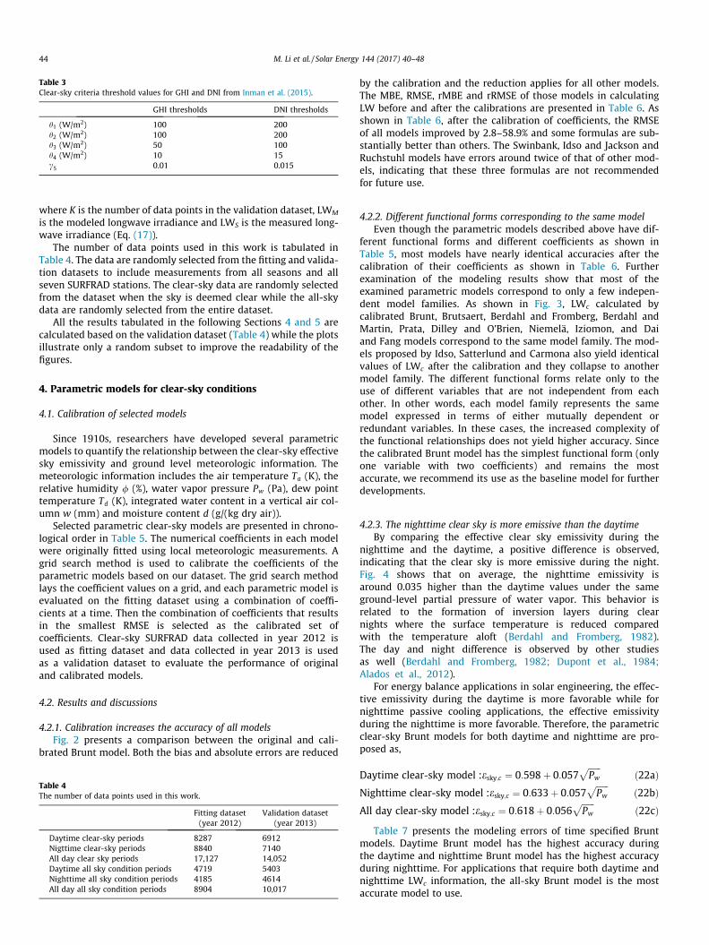
Table 3Clear-sky criteria threshold values for GHI and DNI from Inman et al. (2015).

GHI thresholds DNI thresholds

h1 (W/m2) 100 200h2 (W/m2) 100 200h3 (W/m2) 50 100h4 (W/m2) 10 15c5 0.01 0.015

44 M. Li et al. / Solar Energy 144 (2017) 40–48

where K is the number of data points in the validation dataset, LWM

is the modeled longwave irradiance and LWS is the measured long-wave irradiance (Eq. (17)).

The number of data points used in this work is tabulated inTable 4. The data are randomly selected from the fitting and valida-tion datasets to include measurements from all seasons and allseven SURFRAD stations. The clear-sky data are randomly selectedfrom the dataset when the sky is deemed clear while the all-skydata are randomly selected from the entire dataset.

All the results tabulated in the following Sections 4 and 5 arecalculated based on the validation dataset (Table 4) while the plotsillustrate only a random subset to improve the readability of thefigures.

4. Parametric models for clear-sky conditions

4.1. Calibration of selected models

Since 1910s, researchers have developed several parametricmodels to quantify the relationship between the clear-sky effectivesky emissivity and ground level meteorologic information. Themeteorologic information includes the air temperature Ta (K), therelative humidity / (%), water vapor pressure Pw (Pa), dew pointtemperature Td (K), integrated water content in a vertical air col-umn w (mm) and moisture content d (g/(kg dry air)).

Selected parametric clear-sky models are presented in chrono-logical order in Table 5. The numerical coefficients in each modelwere originally fitted using local meteorologic measurements. Agrid search method is used to calibrate the coefficients of theparametric models based on our dataset. The grid search methodlays the coefficient values on a grid, and each parametric model isevaluated on the fitting dataset using a combination of coeffi-cients at a time. Then the combination of coefficients that resultsin the smallest RMSE is selected as the calibrated set ofcoefficients. Clear-sky SURFRAD data collected in year 2012 isused as fitting dataset and data collected in year 2013 is usedas a validation dataset to evaluate the performance of originaland calibrated models.

4.2. Results and discussions

4.2.1. Calibration increases the accuracy of all modelsFig. 2 presents a comparison between the original and cali-

brated Brunt model. Both the bias and absolute errors are reduced

Table 4The number of data points used in this work.

Fitting dataset(year 2012)

Validation dataset(year 2013)

Daytime clear-sky periods 8287 6912Nigttime clear-sky periods 8840 7140All day clear sky periods 17,127 14,052Daytime all sky condition periods 4719 5403Nighttime all sky condition periods 4185 4614All day all sky condition periods 8904 10,017

by the calibration and the reduction applies for all other models.The MBE, RMSE, rMBE and rRMSE of those models in calculatingLW before and after the calibrations are presented in Table 6. Asshown in Table 6, after the calibration of coefficients, the RMSEof all models improved by 2.8–58.9% and some formulas are sub-stantially better than others. The Swinbank, Idso and Jackson andRuchstuhl models have errors around twice of that of other mod-els, indicating that these three formulas are not recommendedfor future use.

4.2.2. Different functional forms corresponding to the same modelEven though the parametric models described above have dif-

ferent functional forms and different coefficients as shown inTable 5, most models have nearly identical accuracies after thecalibration of their coefficients as shown in Table 6. Furtherexamination of the modeling results show that most of theexamined parametric models correspond to only a few indepen-dent model families. As shown in Fig. 3, LWc calculated bycalibrated Brunt, Brutsaert, Berdahl and Fromberg, Berdahl andMartin, Prata, Dilley and O’Brien, Niemelä, Iziomon, and Daiand Fang models correspond to the same model family. The mod-els proposed by Idso, Satterlund and Carmona also yield identicalvalues of LWc after the calibration and they collapse to anothermodel family. The different functional forms relate only to theuse of different variables that are not independent from eachother. In other words, each model family represents the samemodel expressed in terms of either mutually dependent orredundant variables. In these cases, the increased complexity ofthe functional relationships does not yield higher accuracy. Sincethe calibrated Brunt model has the simplest functional form (onlyone variable with two coefficients) and remains the mostaccurate, we recommend its use as the baseline model for furtherdevelopments.

4.2.3. The nighttime clear sky is more emissive than the daytimeBy comparing the effective clear sky emissivity during the

nighttime and the daytime, a positive difference is observed,indicating that the clear sky is more emissive during the night.Fig. 4 shows that on average, the nighttime emissivity isaround 0.035 higher than the daytime values under the sameground-level partial pressure of water vapor. This behavior isrelated to the formation of inversion layers during clearnights where the surface temperature is reduced comparedwith the temperature aloft (Berdahl and Fromberg, 1982).The day and night difference is observed by other studiesas well (Berdahl and Fromberg, 1982; Dupont et al., 1984;Alados et al., 2012).

For energy balance applications in solar engineering, the effec-tive emissivity during the daytime is more favorable while fornighttime passive cooling applications, the effective emissivityduring the nighttime is more favorable. Therefore, the parametricclear-sky Brunt models for both daytime and nighttime are pro-posed as,

Daytime clear-sky model :esky;c ¼ 0:598þ 0:057ffiffiffiffiffiffiPw

pð22aÞ

Nighttime clear-sky model :esky;c ¼ 0:633þ 0:057ffiffiffiffiffiffiPw

pð22bÞ

All day clear-sky model :esky;c ¼ 0:618þ 0:056ffiffiffiffiffiffiPw

pð22cÞ

Table 7 presents the modeling errors of time specified Bruntmodels. Daytime Brunt model has the highest accuracy duringthe daytime and nighttime Brunt model has the highest accuracyduring nighttime. For applications that require both daytime andnighttime LWc information, the all-sky Brunt model is the mostaccurate model to use.

Fig. 2. Modeled LW with respect to measured LW. (a) Original Brunt model; (b) Calibrated Brunt model.

Table 5Parametric models for clear skies.

Model YearDeveloped

Variables Formulation Original Parameters

Brunt (1932) 1932 Pw (hPa) esky ¼ c1 þ c2ffiffiffiffiffiffiPw

pc1 ¼ 0:52; c2 ¼ 0:065

Swinbank (1963) 1963 Ta (K) esky ¼ c1Tc2a c1 ¼ 9:365� 10�6; c2 ¼ 2

Idso and Jackson (1969) 1969 Ta (K) esky ¼ 1� c1 exp½c2ð273� TaÞc3 � c1 ¼ 0:261; c2 ¼ �7:77� 10�4; c3 ¼ 2Brutsaert (1975) 1975 Pw (hPa), Ta (K) esky ¼ c1 Pw=Tað Þc2 c1 ¼ 1:24; c2 ¼ 1=7

Satterlund (1979) 1979 Pw (hPa), Ta (K) esky ¼ c1½1� expð�PTa=c2w Þ� c1 ¼ 1:08; c2 ¼ 2016

Idso (1981) 1981 Pw (hPa), Ta (K) esky ¼ c1 þ c2Pw expðc3=TaÞÞ c1 ¼ 0:70; c2 ¼ 5:95� 10�5; c3 ¼ 1500Berdahl and Fromberg (1982) 1982 Td (�C) esky ¼ c1 þ c2Td (daytime) c1 ¼ 0:727; c2 ¼ 0:0060Berdahl and Martin (1984) 1984 Td (�C) esky ¼ c1 þ c2 Td=100ð Þ þ c3 Td=100ð Þ2 c1 ¼ 0:711; c2 ¼ 0:56; c3 ¼ 0:73

Prata (1996) 1996 w (g/cm2), Pw (hPa),Ta (K)

esky ¼ 1� ð1þwÞ expð� ffiffiðpc1 þ c2wÞÞ;w ¼ c3 Pw

Tac1 ¼ 1:2; c2 ¼ 3; c3 ¼ 46:5

Dilley and O’brien (1998) 1998 Ta (K), w (kg/m2) esky ¼ c1 þ c2 Ta273:16

� �6 þ c3ffiffiffiffiw25

p� .rT4

a ;w ¼ 4:65 PwTa

c1 ¼ 59:38; c2 ¼ 113:7; c3 ¼ 96:96

Niemelä et al. (2001) 2001 Pw (hPa) esky ¼ c1 þ c2ðPw � c3Þ, if Pw P c3 c1 ¼ 0:72; c2 ¼ 0:009; c3 ¼ 2esky ¼ c1 � c2ðPw � c3Þ, if Pw < c3 c1 ¼ 0:72; c2 ¼ 0:076; c3 ¼ 2

Iziomon et al. (2003) 2003 Pw (hPa), Ta (K) esky ¼ 1� c1 exp �10PwTa

� c1 ¼ 0:35

Ruckstuhl et al. (1984) 2007 w (mm), d (g/kg) esky ¼ c1wc2 ;w ¼ c3d� c4 c1 ¼ 147:8; c2 ¼ 0:26; c3 ¼ 2:40; c4 ¼ 1:60Dai and Fang (2014) 2014 Pw (hPa), Pa (hPa) esky ¼ ðc1 þ c2P

c3w Þ Pa=1013ð Þc4 c1 ¼ 0:48; c2 ¼ 0:17; c3 ¼ 0:22; c4 ¼ 0:45

Carmona et al. (2014) 2014 Ta (K), / (%) esky ¼ �c1 þ c2Ta þ c3/ c1 ¼ 0:34; c2 ¼ 3:36� 10�3; c3 ¼ 1:94� 10�3

M. Li et al. / Solar Energy 144 (2017) 40–48 45

5. Parametric models for all-sky conditions

5.1. Calibration of selected and proposed models

Under all-sky conditions, the downward longwave irradiance isincreased by the radiation emission from clouds (liquid water and/or ice). Therefore, the all-sky parametric models need to includecloud information such as cloud cover fraction (CF) or cloudmodification factor (CMF). In 1999, Crawford and Duchon (1999)developed a parametric model that accounts for the emission ofclouds in the form of,

LW ¼ LWcð1� c1CFc2 Þ þ c3CF

c4rT4a ð23Þ

In the original Crawford and Duchon model, all the four coefficientsc1 � c4 are equal to 1. Other parametric models proposed by

References Konzelmann et al. (1994) and Duarte et al. (2006) wouldalso collapse to this form with different c1 � c4.

A parametric model for daytime all-sky condition was proposedby Bilbao and De Miguel (2007),

LW ¼ LWcð1þ c1CMFc2 Þ ð24Þwhere c1 and c2 are coefficients regressed from local measurements.

Another model proposed by Alados et al. (2012) has the func-tional relation

LW ¼ LWcðc1 � c2ð1� CMFÞÞ ð25Þwhere c1 and c2 are locally fitted coefficients as well.

To account for the modification of LW due to clouds, we proposea comprehensive new model as shown in Eq. (26) where CMF or CFequals to zero corresponds to clear (cloud free) conditions. The first

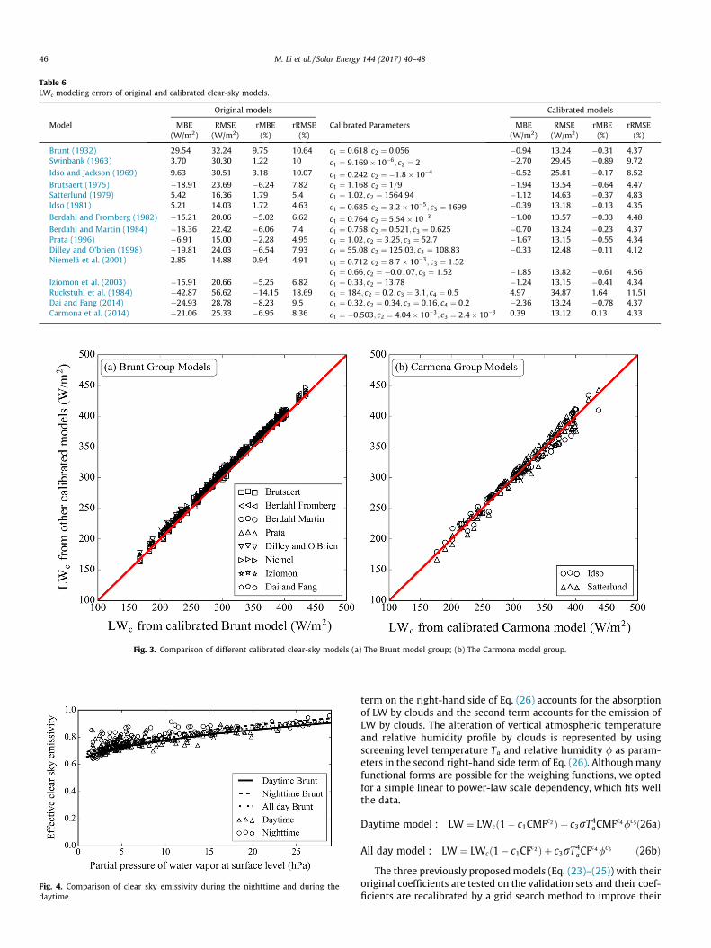
Fig. 3. Comparison of different calibrated clear-sky models (a) The Brunt model group; (b) The Carmona model group.

Table 6LWc modeling errors of original and calibrated clear-sky models.

Original models Calibrated models

Model MBE(W/m2)

RMSE(W/m2)

rMBE(%)

rRMSE(%)

Calibrated Parameters MBE(W/m2)

RMSE(W/m2)

rMBE(%)

rRMSE(%)

Brunt (1932) 29.54 32.24 9.75 10.64 c1 ¼ 0:618; c2 ¼ 0:056 �0.94 13.24 �0.31 4.37Swinbank (1963) 3.70 30.30 1.22 10 c1 ¼ 9:169� 10�6; c2 ¼ 2 �2.70 29.45 �0.89 9.72

Idso and Jackson (1969) 9.63 30.51 3.18 10.07 c1 ¼ 0:242; c2 ¼ �1:8� 10�4 �0.52 25.81 �0.17 8.52

Brutsaert (1975) �18.91 23.69 �6.24 7.82 c1 ¼ 1:168; c2 ¼ 1=9 �1.94 13.54 �0.64 4.47Satterlund (1979) 5.42 16.36 1.79 5.4 c1 ¼ 1:02; c2 ¼ 1564:94 �1.12 14.63 �0.37 4.83Idso (1981) 5.21 14.03 1.72 4.63 c1 ¼ 0:685; c2 ¼ 3:2� 10�5; c3 ¼ 1699 �0.39 13.18 �0.13 4.35

Berdahl and Fromberg (1982) �15.21 20.06 �5.02 6.62 c1 ¼ 0:764; c2 ¼ 5:54� 10�3 �1.00 13.57 �0.33 4.48

Berdahl and Martin (1984) �18.36 22.42 �6.06 7.4 c1 ¼ 0:758; c2 ¼ 0:521; c3 ¼ 0:625 �0.70 13.24 �0.23 4.37Prata (1996) �6.91 15.00 �2.28 4.95 c1 ¼ 1:02; c2 ¼ 3:25; c3 ¼ 52:7 �1.67 13.15 �0.55 4.34Dilley and O’brien (1998) �19.81 24.03 �6.54 7.93 c1 ¼ 55:08; c2 ¼ 125:03; c3 ¼ 108:83 �0.33 12.48 �0.11 4.12Niemelä et al. (2001) 2.85 14.88 0.94 4.91 c1 ¼ 0:712; c2 ¼ 8:7� 10�3; c3 ¼ 1:52

c1 ¼ 0:66; c2 ¼ �0:0107; c3 ¼ 1:52 �1.85 13.82 �0.61 4.56Iziomon et al. (2003) �15.91 20.66 �5.25 6.82 c1 ¼ 0:33; c2 ¼ 13:78 �1.24 13.15 �0.41 4.34Ruckstuhl et al. (1984) �42.87 56.62 �14.15 18.69 c1 ¼ 184; c2 ¼ 0:2; c3 ¼ 3:1; c4 ¼ 0:5 4.97 34.87 1.64 11.51Dai and Fang (2014) �24.93 28.78 �8.23 9.5 c1 ¼ 0:32; c2 ¼ 0:34; c3 ¼ 0:16; c4 ¼ 0:2 �2.36 13.24 �0.78 4.37Carmona et al. (2014) �21.06 25.33 �6.95 8.36 c1 ¼ �0:503; c2 ¼ 4:04� 10�3; c3 ¼ 2:4� 10�3 0.39 13.12 0.13 4.33

Fig. 4. Comparison of clear sky emissivity during the nighttime and during thedaytime.

46 M. Li et al. / Solar Energy 144 (2017) 40–48

term on the right-hand side of Eq. (26) accounts for the absorptionof LW by clouds and the second term accounts for the emission ofLW by clouds. The alteration of vertical atmospheric temperatureand relative humidity profile by clouds is represented by usingscreening level temperature Ta and relative humidity / as param-eters in the second right-hand side term of Eq. (26). Althoughmanyfunctional forms are possible for the weighing functions, we optedfor a simple linear to power-law scale dependency, which fits wellthe data.

Daytime model : LW ¼ LWcð1� c1CMFc2 Þ þ c3rT4aCMFc4/c5ð26aÞ

All day model : LW ¼ LWcð1� c1CFc2 Þ þ c3rT4

aCFc4/c5 ð26bÞ

The three previously proposed models (Eq. (23)–(25)) with theiroriginal coefficients are tested on the validation sets and their coef-ficients are recalibrated by a grid search method to improve their

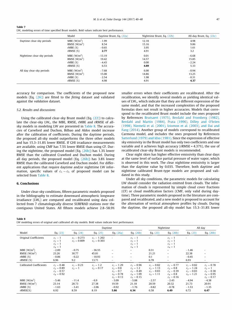
Table 7LWc modeling errors of time specified Brunt models. Bold values indicate best performance.

Model Daytime Brunt, Eq. (22a) Nighttime Brunt, Eq. (22b) All-day Brunt, Eq. (22c)

Daytime clear-sky periods MBE (W/m2) �1.99 12.18 4.98RMSE (W/m2) 8.54 15.16 9.86rMBE (%) �0.65 3.95 1.61rRMSE (%) 2.77 4.91 3.2

Nighttime clear-sky periods MBE (W/m2) �13.19 0.01 �6.68RMSE (W/m2) 19.42 14.57 15.85rMBE (%) �4.43 0.00 �2.24rRMSE (%) 6.53 4.89 5.33

All day clear-sky periods MBE (W/m2) �7.68 6.00 �0.94RMSE (W/m2) 15.08 14.86 13.25rMBE (%) �2.54 1.98 �0.31rRMSE (%) 4.98 4.91 4.37

M. Li et al. / Solar Energy 144 (2017) 40–48 47

accuracy for comparison. The coefficients of the proposed newmodels (Eq. (26)) are fitted to the fitting dataset and validatedagainst the validation dataset.

5.2. Results and discussions

Using the calibrated clear-sky Brunt model (Eq. (22)) to calcu-late the clear-sky LWc, the MBE, RMSE, rMBE and rRMSE of all-sky models in modeling LW are presented in Table 8. The accura-cies of Carwford and Duchon, Bilbao and Aldos model increaseafter the calibration of coefficients. During the daytime periods,the proposed all-sky model outperforms the three other modelsand has 15.3–31.8% lower RMSE. If GHI irradiance measurementsare available, using CMF has 7.5% lower RMSE than using CF. Dur-ing the nighttime, the proposed model (Eq. (26b)) has 1.3% lowerRMSE than the calibrated Crawford and Duchon model. Duringall day periods, the proposed model (Eq. (26b)) has 3.8% lowerRMSE than the calibrated Carwford and Duchon model. For differ-ent applications that require daytime and/or nighttime LW infor-mation, specific values of c1 � c5 of proposed model can beselected from Table 8.

6. Conclusions

Under clear-sky conditions, fifteen parametric models proposedin the bibliography to estimate downward atmospheric longwaveirradiance (LWc) are compared and recalibrated using data col-lected from 7 climatologically diverse SURFRAD stations over thecontiguous United States. All fifteen models achieve 2.8–58.9%

Table 8LW modeling errors of original and calibrated all-sky models. Bold values indicate best pe

Daytime

Model Eq. (23) Eq. (24) Eq. (25) Eq. (26

Original Coefficients c1 ¼ 1c2 ¼ 1c3 ¼ 1c4 ¼ 1

c1 ¼ 0:273c2 ¼ 0:809

c1 ¼ 1:202c2 ¼ 0:303

-

MBE (W/m2) �2.89 �0.75 �36.55 –RMSE (W/m2) 23.26 30.77 45.81 –rMBE (%) �0.86 �0.22 �10.93 –rRMSE (%) 6.96 9.2 13.71 –

Calibrated Coefficients c1 ¼ 0:48c2 ¼ 0:89c3 ¼ 0:57c4 ¼ 0:92

c1 ¼ 0:23c2 ¼ 1

c1 ¼ 1:2c2 ¼ 0:17

c1 ¼ 1:2c2 ¼ 0:8c3 ¼ 0:7c4 ¼ 0:7c5 ¼ 0:1

MBE (W/m2) �5.46 �11.4 �6.9 �3.09RMSE (W/m2) 23.14 28.73 27.38 19.59rMBE (%) �1.63 �3.41 �2.06 �0.92rRMSE(%) 6.92 8.59 8.19 5.86

smaller errors when their coefficients are recalibrated. After therecalibration, we identify several models as yielding identical val-ues of LWc, which indicate that they are different expression of thesame model, and that the increased complexities of the proposedformulas does not result in higher accuracies. Models that corre-spond to the recalibrated Brunt model include the ones proposedby References Brutsaert (1975), Berdahl and Fromberg (1982),Berdahl and Martin (1984), Prata (1996), Dilley and O’brien(1998), Niemelä et al. (2001), Iziomon et al. (2003), and Dai andFang (2014). Another group of models correspond to recalibratedCarmona model, and includes the ones proposed by ReferencesSatterlund (1979) and Idso (1981). Since the expression of effectivesky emissivity in the Brunt model has only two coefficients and onevariable and it achieves high accuracy (rRMSE = 4.37%), the use ofrecalibrated clear-sky Brunt models is recommended.

Clear night skies has higher effective emissivity than clear daysat the same level of surface partial pressure of water vapor, whichis observed in this work. The clear nighttime emissivity is largerthan the daytime value by 0.035. Therefore, both daytime andnighttime calibrated Brunt-type models are proposed and vali-dated in this study.

Under all sky conditions, the parametric models for calculatingLW should consider the radiation emitted from clouds. The infor-mation of clouds is represented by simple cloud cover fractions(CF) or cloud modification factors (CMF, only valid during day-time). Three parametric models proposed in the literature are com-pared and recalibrated, and a newmodel is proposed to account forthe alternation of vertical atmosphere profiles by clouds. Duringthe daytime, the proposed all-sky model has 15.3–31.8% lower

rformance.

Nighttime All day

a) Eq. (26b) Eq. (23) Eq. (26b) Eq. (23) Eq. (26b)

c1 ¼ 1c2 ¼ 1c3 ¼ 1c4 ¼ 1

– c1 ¼ 1c2 ¼ 1c3 ¼ 1c4 ¼ 1

-

– 0.31 – �1.46 -– 21.21 – 22.38 –– 0.1 – �0.45 –– 6.78 – 6.93 –

9

83

c1 ¼ 0:96c2 ¼ 1:2c3 ¼ 0:49c4 ¼ 1:09c5 ¼ 0:15

c1 ¼ 0:82c2 ¼ 1:13c3 ¼ 0:83c4 ¼ 1:11

c1 ¼ 0:77c2 ¼ 0:8c3 ¼ 0:39c4 ¼ 0:8c5 ¼ 0:16

c1 ¼ 0:82c2 ¼ 1:24c3 ¼ 0:83c4 ¼ 1:21

c1 ¼ 0:78c2 ¼ 1c3 ¼ 0:38c4 ¼ 0:95c5 ¼ 0:17

�5.88 �2.57 �2.43 �4.94 �4.3821.18 20.59 20.32 21.73 20.91�1.76 �0.82 �0.78 �1.53 �1.356.34 6.58 6.49 6.72 6.47

48 M. Li et al. / Solar Energy 144 (2017) 40–48

RMSE than the other three calibrated models. If GHI irradiancemeasurements are available, using CMF has 7.5% lower RMSE thanusing CF. During the nighttime and all day periods, the proposedmodel yields 1.3–3.8% lower RMSE than the recalibrated Crawfordand Duchon model. For different applications that require LWinformation during daytime and/or nighttime, coefficients of theproposed model can be selected for use.

The main contributions of this work are: (1) We propose novelaccurate parametric models to calculate 1-min averaged down-ward atmospheric longwave irradiance under both clear-sky andall-sky conditions. (2) The coefficients of the proposed modelsshould be considered more universal, since data from seven clima-tologically diverse stations (rather than one or two particular loca-tions) are used. (3) We also determined that several clear-skyparametric models proposed recently are equivalent.

Acknowledgments

The authors gratefully acknowledge the partial support by theCalifornia Energy Commission EPIC PON-13-303 program, whichis managed by Dr. Silvia Palma-Rojas. The authors also thankfulto Dr. Chi-Han Cheng from the University of Central Florida fordownloading the ASOS cloud fraction data.

Appendix A

Adapted from Ref.Kasten and Young (1989); Ineichen and Perez(2002); Ineichen (2006); Ineichen (2008); Inman et al. (2015), theclear sky GHI is expressed as,

GHIc ¼ c1I0 sinðaeÞ � e0:01m1:8�c2mðf 1þf 2ðTL�1ÞÞ

where c1; c2; f 1 and f 2 are altitude correction coefficients, I0 (W/m2)is the extraterrestrial irradiance, ae (�) is the solar elevation angle,mis the air mass and TL is the Linke turbidity factor. The clear sky DNIis expressed as,

DNIc ¼ 0:664þ 0:163f 1

� �I0 � e�0:09mðTL�1Þ

The altitude correction coefficients are:

c1 ¼ 5:09� 10�5Altþ 0:868

c2 ¼ 3:92� 10�5Altþ 0:0387

f 1 ¼ e�Alt=8000

f 2 ¼ e�Alt=1250

with Alt (m) is the altitude. The extraterrestrial irradiance I0 isexpressed as,

I0 ¼ 1367:7 1þ 0:033 cos2p

365:25DOY

� �� �

with DOY is the day of year. The air mass m is expressed as a func-tion of solar elevation angle,

1m

¼ sinae þ 0:15 ae180p

þ 3:885� ��1:253

The Linke turbidity factor TL is extracted from monthly Link turbid-ity images. The above model can be used to calculated 1-min aver-aged clear-sky GHI and DNI.

References

Alados, I., Foyo-Moreno, I., Alados-Arboledas, L., 2012. Estimation of downwellinglongwave irradiance under all-sky conditions. Int. J. Climatol. 32 (5), 781–793.

Alduchov, O.A., Eskridge, R.E., 1996. Improved Magnus form approximation ofsaturation vapor pressure. J. Appl. Meteorol. 35 (4), 601–609.

Berdahl, P., Fromberg, R., 1982. The thermal radiance of clear skies. Sol. Energy 29(4), 299–314.

Berdahl, P., Martin, M., 1984. Emissivity of clear skies. Sol. Energy 32 (5), 663–664.Bilbao, J., De Miguel, A.H., 2007. Estimation of daylight downward longwave

atmospheric irradiance under clear-sky and all-sky conditions. J. Appl.Meteorol. Climatol. 46 (6), 878–889.

Brunt, D., 1932. Notes on radiation in the atmosphere. I. Quart. J. Roy. Meteorol. Soc.58 (247), 389–420.

Brutsaert, W., 1975. On a derivable formula for long-wave radiation from clearskies. Water Resour. Res. 11 (5), 742–744.

Carmona, F., Rivas, R., Caselles, V., 2014. Estimation of daytime downward longwaveradiation under clear and cloudy skies conditions over a sub-humid region.Theoret. Appl. Climatol. 115 (1–2), 281–295.

Crawford, T.M., Duchon, C.E., 1999. An improved parameterization for estimatingeffective atmospheric emissivity for use in calculating daytime downwellinglongwave radiation. J. Appl. Meteorol. 38 (4), 474–480.

Dai, Q., Fang, X., 2014. A new model for atmospheric radiation under clear skycondition at various altitudes. Adv. Space Res. 54 (6), 1044–1048.

Dilley, A.C., O’brien, D.M., 1998. Estimating downward clear sky long-waveirradiance at the surface from screen temperature and precipitable water.Quart. J. Roy. Meteorol. Soc. 124 (549), 1391–1401.

Duarte, H.F., Dias, N.L., Maggiotto, S.R., 2006. Assessing daytime downwardlongwave radiation estimates for clear and cloudy skies in Southern Brazil.Agric. Forest Meteorol. 139 (3), 171–181.

Dupont, J.-C., Haeffelin, M., Drobinski, P., Besnard, T., 1984. Parametric model toestimate clear-sky longwave irradiance at the surface on the basis of verticaldistribution of humidity and temperature. J. Geophys. Res.: Atmos. 113 (D7).

Eicker, U., Dalibard, A., 2011. Photovoltaic–thermal collectors for night radiativecooling of buildings. Sol. Energy 85 (7), 1322–1335.

Golden Gate Weather Service, 2016. El Niño and La Niña years and intensities.<http://ggweather.com/enso/oni.htm>.

Idso, S.B., 1981. A set of equations for full spectrum and 8-to 14-lm and 10.5-to12.5-lm thermal radiation from cloudless skies. Water Resources Res. 17 (2),295–304.

Idso, S.B., Jackson, R.D., 1969. Thermal radiation from the atmosphere. J. Geophys.Res. 74 (23), 5397–5403.

Ineichen, P., 2006. Comparison of eight clear sky broadband models against 16independent data banks. Sol. Energy 80 (4), 468–478.

Ineichen, P., 2008. Conversion function between the linke turbidity and theatmospheric water vapor and aerosol content. Sol. Energy 82 (11), 1095–1097.

Ineichen, P., Perez, R., 2002. A new airmass independent formulation for the Linketurbidity coefficient. Sol. Energy 73 (3), 151–157.

Inman, R.H., Edson, J.G., Coimbra, C.F.M., 2015. Impact of local broadband turbidityestimation on forecasting of clear sky direct normal irradiance. Sol. Energy 117,125–138.

Iowa State University of Science and Technology, 2016. ASOS-AWOS-METAR datadownload. <https://mesonet.agron.iastate.edu/request/download.phtml>.

Iziomon, M.G., Mayer, H., Matzarakis, A., 2003. Downward atmospheric longwaveirradiance under clear and cloudy skies: measurement and parameterization. J.Atmos. Sol. Terr. Phys. 65 (10), 1107–1116.

Kasten, F., Young, A.T., 1989. Revised optical air mass tables and approximationformula. Appl. Opt. 28 (22), 4735–4738.

Konzelmann, T., van de Wal, R.S., Greuell, W., Bintanja, R., Henneken, E.A., Abe-Ouchi, A., 1994. Parameterization of global and longwave incoming radiation forthe Greenland Ice Sheet. Global Planet. Change 9 (1), 143–164.

Maghrabi, A., Clay, R., 2011. Nocturnal infrared clear sky temperatures correlatedwith screen temperatures and GPS-derived PWV in Southern Australia. EnergyConvers. Manage. 52 (8), 2925–2936.

Mills, A.F., Coimbra, C.F.M., 2015. Basic Heat and Mass Transfer. TemporalPublishing, San Diego, CA.

National Oceanic and Atmospheric Administration, 1998. Automated surfaceobserving system user’s guide. <http://www.nws.noaa.gov/asos/pdfs/aum-toc.pdf>.

National Oceanic and Atmospheric Administration, 2015. SURFRAD Network.<http://www.esrl.noaa.gov/gmd/grad/surfrad/>.

Niemelä, S., Räisänen, P., Savijärvi, H., 2001. Comparison of surface radiative fluxparameterizations: Part I: Longwave radiation. Atmos. Res. 58 (1), 1–18.

Prata, A.J., 1996. A new long-wave formula for estimating downward clear-skyradiation at the surface. Quart. J. Roy. Meteorol. Soc. 122 (533), 1127–1151.

Reno, M.J., Hansen, C.W., Stein, J.S., 2012. Global horizontal irradiance clear skymodels: implementation and analysis, SANDIA report SAND2012-2389.

Ruckstuhl, C., Philipona, R., Morland, J., Ohmura, A., 1984. Observed relationshipbetween surface specific humidity, integrated water vapor, and longwavedownward radiation at different altitudes. J. Geophys. Res.: Atmos. 112 (D3).

Satterlund, D.R., 1979. An improved equation for estimating long-wave radiationfrom the atmosphere. Water Resour. Res. 15 (6), 1649–1650.

Swinbank, W.C., 1963. Long-wave radiation from clear skies. Quart. J. Roy. Meteorol.Soc. 89 (381), 339–348.

Tang, R., Etzion, Y., Meir, I.A., 2004. Estimates of clear night sky emissivity in theNegev Highlands, Israel. Energy Convers. Manage. 45 (11), 1831–1843.

Zaversky, F., García-Barberena, J., Sánchez, M., Astrain, D., 2013. Transient moltensalt two-tank thermal storage modeling for CSP performance simulations. Sol.Energy 93, 294–311.