on the design of a boolean-network robot swarm:...
TRANSCRIPT

ALMA MATER STUDIORUM - UNIVERSITA DI BOLOGNA
SECONDA FACOLTA DI INGEGNERIA
Corso di Laurea Magistrale in
Ingegneria Informatica
ON THE DESIGN OF ABOOLEAN-NETWORK ROBOT SWARMCOLLECTIVE RECOGNITION OF GROUND PATTERNS
Tesi di Laurea elaborata nel corso di:
Intelligenza Artificiale L-M
Tesi di Laurea di:
Davide Vichi
Relatore:
Prof. Andrea Roli
Correlatori:
Dott. Ing. Mauro Birattari
Ing. Carlo Pinciroli
Prof. Marco Dorigo
Anno Accademico 2011/2012
Sessione I

KEY WORDS
Boolean Networks
Swarm Robotics
Metaheuristics


Acknowledgements
First of all, I would like to thank my teacher Andrea Roli, who was able
to nourish and support my passion since I attended the university courses.
This year, he has given to me the opportunity to undertake this magnificent
experience which has already changed my life.
I thank also Marco Dorigo for giving me the possibility to work in IRIDIA
and Mauro Birattari for his support and optimism.
Very thanks to my supervisor Carlo Pinciroli, someone special. Despite
his thousands commitments, always helped me with a smile even facing big
troubles.
I thank all the Iridians: kind guys with whom I shared lunches in can-
teens, dinners, beers, opinions and laughs. I also greet my office mates,
masters students like me, Andreea, Simon and Mikael. Good luck for your
future, I hope to see you again.
I thank my fellows Matteo and Lorenzo, who have given to me a coat to
acclimate in Brussels. Thanks to them I discovered delicious Belgian beers.
I thank my fellow Mattia who just back from the same experience two years
ago, who gave me encouragement in undertaking this adventure. You were
right, it was worth it.
I was pleasantly surprised by the solidarity between ethnic groups that
populate Brussels. In particular, I warmly thank my Czech landlady Jara
who treated me like a son and taught me to speak French. I thank Claudia,
the mexican landlady of Matteo and Lorenzo for her hospitality and for our
discussions washed by tequila.

vi Acknowledgements
Heartfelt thanks to my girlfriend Giulia, who has patiently waited me for
6 months, putting herself aside and fully supporting my convictions. I hope
that what I learned can help us to better face the challenges in our life.
Finally, I thank my family for allowing me to study and for their encour-
agement during difficult times.
I still remember the first time I was given a personal computer. I was
six and the first thing that I asked was “Can I write my name?”. I hope
that now, after some years of studies, I can be able to respond to also more
interesting questions.
Contents
Acknowledgements v
1 Introduction 1
2 Boolean Networks 5
2.1 Introduction . . . . . . . . . . . . . . . . . . . . . . . . . . . . 5
2.2 Boolean Network Dynamics . . . . . . . . . . . . . . . . . . . 6
2.3 Random Boolean Networks . . . . . . . . . . . . . . . . . . . . 9
2.4 Boolean Network Design . . . . . . . . . . . . . . . . . . . . . 12
3 Boolean Networks Robotics 15
3.1 Basics . . . . . . . . . . . . . . . . . . . . . . . . . . . . . . . 15
3.2 Methodology . . . . . . . . . . . . . . . . . . . . . . . . . . . 17
3.2.1 BN-Robot Coupling . . . . . . . . . . . . . . . . . . . 17
3.2.2 BN-Controller Design . . . . . . . . . . . . . . . . . . . 18
3.2.3 Iterated Local Search . . . . . . . . . . . . . . . . . . . 20
3.3 Related Work . . . . . . . . . . . . . . . . . . . . . . . . . . . 22
3.3.1 A Proof of Concept . . . . . . . . . . . . . . . . . . . . 22
3.3.2 Improving the Search Method . . . . . . . . . . . . . . 23
3.3.3 State Space Analysis . . . . . . . . . . . . . . . . . . . 24
4 Task Description 25
4.1 Task Requirements . . . . . . . . . . . . . . . . . . . . . . . . 26
4.2 Description . . . . . . . . . . . . . . . . . . . . . . . . . . . . 26
viii CONTENTS
4.2.1 Robots . . . . . . . . . . . . . . . . . . . . . . . . . . . 27
4.2.2 Environment . . . . . . . . . . . . . . . . . . . . . . . 32
4.2.3 Initial Conditions . . . . . . . . . . . . . . . . . . . . . 33
4.3 Distributed Computation . . . . . . . . . . . . . . . . . . . . . 34
4.3.1 Sensors Networks . . . . . . . . . . . . . . . . . . . . . 34
4.3.2 Cellular Automata . . . . . . . . . . . . . . . . . . . . 36
5 Preliminary Experiments 39
5.1 Initial Setting . . . . . . . . . . . . . . . . . . . . . . . . . . . 39
5.2 First Step: Stochastic Descent Results . . . . . . . . . . . . . 42
5.3 Second Step: Iterated Local Search . . . . . . . . . . . . . . . 42
5.3.1 Results . . . . . . . . . . . . . . . . . . . . . . . . . . . 44
5.4 Third Step: Iterated Local Search with Average as Objective
Function . . . . . . . . . . . . . . . . . . . . . . . . . . . . . . 45
5.4.1 Results . . . . . . . . . . . . . . . . . . . . . . . . . . . 46
5.5 Fourth Step: Objective Function H . . . . . . . . . . . . . . . 47
5.5.1 Two Different Batches of Experiments . . . . . . . . . 50
5.5.2 Results . . . . . . . . . . . . . . . . . . . . . . . . . . . 51
5.6 Fifth Step: Tuning Parameters . . . . . . . . . . . . . . . . . . 52
5.6.1 Results . . . . . . . . . . . . . . . . . . . . . . . . . . . 53
6 A Simpler Case 55
6.1 Description . . . . . . . . . . . . . . . . . . . . . . . . . . . . 55
6.2 First Results . . . . . . . . . . . . . . . . . . . . . . . . . . . . 57
6.3 Results Without Rotational Symmetry . . . . . . . . . . . . . 59
6.4 A New Instance of the Problem . . . . . . . . . . . . . . . . . 61
6.5 Results With Japanese Flag . . . . . . . . . . . . . . . . . . . 63
7 Conclusion 65
A Interacting Boolean Networks 69
Bibliography 76

CONTENTS ix
List of figures 78
List of tables 79

x CONTENTS
1. Introduction
Under the 7th RTD Framework Programme of the European Commission,
several grant agreements (about 75) fall in the remit of the ICT Challenge
“Cognitive systems and robotics”. The phenomenon demonstrates the still
lively interest in artificial intelligence for the European scientific community.
In particular, such projects concern issues about endowing artificial systems
with cognitive capabilities including: recognition, reasoning and planning,
learning and adaptation. The term “cognitive capabilities” is used with good
justification to indicate skills that can make a robotic device able to control
its own actions. Simple cognitive capabilities like establishing and recognising
patterns are prerequisites for higher level operations like conceptualization,
reasoning, planning, intelligent control and complex goal-oriented behaviour.
Moreover, the trend outlined in Strategic Research Agenda (SRA) issued
by the European Robotics Platform in 2009, predicts that by 2020 robots
should be programmable by learning (e.g., from observation or imitation).
Such systems will operate in non-deterministic environments and will regu-
larly be confronted with novelty and change. In order to work robustly and
adaptively, they not only have to be able to extract information from their
environment but also to reason and learn about it [44].
To accomplish such features, the employment of automatic design proce-
dures is needed since such procedures can make the process more robust and
flexible with respect to a customised one.
In this work, we treat the automatic design process as a search problem
2 Introduction
identifying two main components: the model that represents the robot be-
haviour and the optimisation algorithm that shapes the model according to
specific requirements. Generally, the most commonly used model is the arti-
ficial neural network (ANN) which attempts to simulate either the structure
or functional aspects of the biological central nervous system. ANNs and
genetic regulatory networks in general, have interesting features like robust-
ness and flexibility typical of biological systems. For these reasons, ANNs are
used in the field of Evolutionary Robotics where the network is trained by
means of techniques inspired by the Darwinian evolution. However, because
of their complexity, it is impossible to analyse the solutions found and to
reverse-engineer them.
We can try to overcome the problem using a simpler model of genetic reg-
ulatory networks called Boolean network (BN). BNs have been introduced by
Stuart Kauffmann in 1969 in order to study the mechanisms of evolutionary
processes in nature. With their compactness and simplicity we can never-
theless obtain complex behaviour and, moreover, we can study their internal
dynamics.
The second element of the design process concerns the optimisation al-
gorithm. An appropriate choice can be a specific metaheuristic technique
which, exploring immense search spaces, can find a viable solution in a lim-
ited amount of time.
In this work, developed in collaboration with the Institut de Recherches
Interdisciplinaires et de Developpements en Intelligence Artificielle (IRIDIA)
of the Universite Libre de Bruxelles, we apply the automatic methodologies
to a swarm of BN-controlled robots in order to obtain a specific collective
behaviour. Until this moment, the design in swarm robotics has been empir-
ical, tailored to the specific case. However, because of the growing interest
of the research in this field, a more formal methodology is needed in order
to engineer the design of such systems.
Our goal is to program a set of robots with same controllers, in such a way
that they collectively can decide a specific action to perform in accordance
3
with the environment. The environmental features are distributed and this
make the communication necessary to accomplish the task.
The specific task concerns the recognition of two different patterns drawn
on the floor. The robots are placed in order to uniformly covering all the
peculiarities that emerge from the floor. Robots must reach a consensus only
using local communication and signaling their status through the LEDs.
At first, we validate the automatic design methodology on a given instance
of the problem; this is necessary for determining a suitable optimisation al-
gorithm and a good evaluation criterion for the swarm. Subsequently, the
methodology is applied on a simpler case to better investigate the factors
that can increase the performance.
The abstract scenario depicted in our work is only a simple example of
swarm robotics applications which, however, can provide a proof of concept
for more concrete applications (e.g., the exploration of hostile environments
such as oceans, Mars, human body, etc.).
The thesis is structured as follows:
In Chapter 2 we introduce the Boolean networks as model used for rep-
resenting the robot behaviour. We focus on their dynamics detailing also
the analysis of a special kind of BNs used in our experiments: the Random
Boolean Networks. Finally, we provide an overview of previous works about
BNs design.
In Chapter 3 we define the concept of Boolean Network Robotics relying
on the basics of general robotics. We depict the methodology in all its as-
pects and we report recent studies about this field.
Chapter 4 contains the description of the task highlighting the main
emerging aspects, the description of the chosen robots, environments and
initial conditions for each experiment. We also include a brief overview on
the research areas which partially deal the same issues.
In Chapter 5 we report a sequence of preliminary experiments discussing

4 Introduction
for each case the correlations between the achieved results and the chosen
experimental settings.
In Chapter 6 we simplify the problem for a deeper study of the swarm
behaviour. In particular, we focus our analysis on the exchanged communi-
cations among robots.
Finally, Chapter 7 draws some conclusions and gives an outlook for future
works.

2. Boolean Networks
In this chapter we define the Boolean networks as model to represent the
robot behaviour. After a brief introduction in Sec. 2.1, we discuss their
dynamics in Sec. 2.2 while in Sec. 2.3 we focus on a special kind of BN used
in our experiments: the Random Boolean Network. Section 2.4 reports a
brief of previous works on BNs design.
2.1 Introduction
Boolean Networks (BNs) have been introduced by Stuart Kauffman in 1969
[23] as a simplified model of genetic regulatory networks (GRN) and as an
abstraction of complex systems in order to study the mechanisms of evolu-
tionary processes in nature. Despite their simplicity, BNs are very important
because, for many systems, the on-off Boolean idealization is either accurate
or the best idealization of the nonlinear behaviour of the components in the
system [27].
BNs consist of binary variables, each with two possible states (1 or 0).
The variables are connected such that the activity of each element is gov-
erned by the prior activity of some elements according to a Boolean switching
function. The set of these variables is structured like a directed graph with N
nodes. Each node xi has K ingoing arcs and an associated Boolean variable.
The values of the variables are determined by the function fi = (x1, . . . , xK)

6 Boolean Networks
X1
X2
X3
X2 OR X3
X1 AND X2
X1 NOR X3
Figure 2.1: An example of Boolean Network with N = 3 and K = 2.
where the arguments are the Boolean variable value of the nodes whose out-
going arcs are connected to i. A simple example of BN is showed in Fig. 2.1.
We call state of the BN the sequence of the Boolean variable values
s(t) = (x1(t), . . . , xN(t)) in a given instant of time t. Since a Boolean vari-
able can assume only two different values, the state space size is finite (2N)
and the dynamic behaviour is characterized by a sequence of state updates.
Furthermore, several kinds of update rules and dynamics have been pro-
posed [19] like synchronous (the Boolean variables are all updated at the
same time), asynchronous deterministic (variables do not change their states
all at the same moment, but some do it earlier than others) asynchronous
non-deterministic (not only the nodes do not march in step but these nodes
are non-deterministically updated) etc... The one we consider in this thesis
is synchronous with a deterministic nodes updating.
2.2 Boolean Network Dynamics
The state space of Boolean networks is discrete. Thus, it is possible to enu-
merate all the possible states of the network and study interesting dynamics

2.2 Boolean Network Dynamics 7
X1
X2
X3
X2 OR X3
X1 AND X2
X1 NOR X3
X1 X2 X3 X1 X2 X3
0 0 0 0 1 0
0 0 1 1 0 0
0 1 0 1 1 0
0 1 1 1 0 0
1 0 0 0 0 0
1 0 1 1 0 0
1 1 0 1 0 1
1 1 1 1 0 1
t t+1
Figure 2.2: The table describes the dynamics of the BN showing the successor of each
state.
using concepts such as state (or phase) space, trajectories, attractors and
basins of attraction [6].
Since the state space is finite and the dynamics are deterministic, the
state succession assumes this structure:
• When the BN starts its progress, the trajectory (i.e., the evolution of
the BN into the state space) is a succession in which each state is
different from all the previous ones. This sequence of different states
is called transient and the number of states of the transient is called
lenght of the transient. The transient can have length 0.
• Since the network dynamics are deterministic and the state space is
finite, eventually a sequence of states will be repeated. Such sequences
are named attractors of the BN and they can be classified in cyclic
attractors with period t > 1 or point attractors whether t = 1. Point
attractors are also known as fixed points. The set of states that leads
towards an attractor is named basin of attraction.
8 Boolean Networks
X 1
X 2
X 3
AND
OR
OR
(a)
100
011110
101
111
001 010
000
(b)
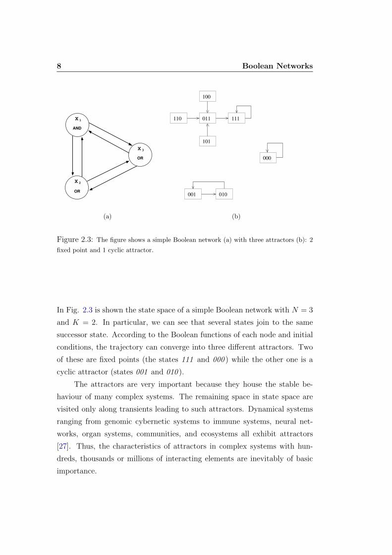
Figure 2.3: The figure shows a simple Boolean network (a) with three attractors (b): 2
fixed point and 1 cyclic attractor.
In Fig. 2.3 is shown the state space of a simple Boolean network with N = 3
and K = 2. In particular, we can see that several states join to the same
successor state. According to the Boolean functions of each node and initial
conditions, the trajectory can converge into three different attractors. Two
of these are fixed points (the states 111 and 000 ) while the other one is a
cyclic attractor (states 001 and 010 ).
The attractors are very important because they house the stable be-
haviour of many complex systems. The remaining space in state space are
visited only along transients leading to such attractors. Dynamical systems
ranging from genomic cybernetic systems to immune systems, neural net-
works, organ systems, communities, and ecosystems all exhibit attractors
[27]. Thus, the characteristics of attractors in complex systems with hun-
dreds, thousands or millions of interacting elements are inevitably of basic
importance.
2.3 Random Boolean Networks 9
2.3 Random Boolean Networks
Starting from the original definition of BN, many variants exist that dif-
fer according to dynamics and updating rules. The most studied are the
Random Boolean Networks (RBNs). RBNs have been used to model living
organisms to provide evidence over the hypothesis that such entities could
be constructed through processes that display some degree of randomness
rather than being precisely programmed [23]. Because of their peculiarities,
RBNs have been also used as models in many different areas, such as evolu-
tionary theory, mathematics, sociology, neural networks, robotics, and music
generation [19].
RBNs are a generalization of Boolean cellular automata (CA) [47], where
the state of each node is not affected necessarily by its neighbours, but po-
tentially by any node in the network. Differently from the general model pre-
sented in Sec. 2.1, RBNs presents randomly generated Boolean functions and
connections among nodes. If we try to imagine all possible networks, for each
node there will be 22K possible functions [21]. Each node has N !/(N −K)!
possible ordered combinations for K different links. Therefore all the possible
networks for given N and K will be:
(22KN !
(N −K)!
)N
(2.1)
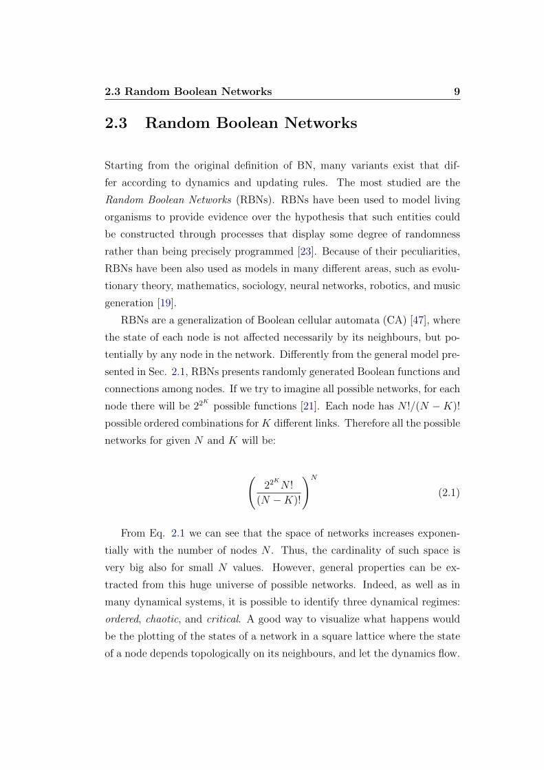
From Eq. 2.1 we can see that the space of networks increases exponen-
tially with the number of nodes N . Thus, the cardinality of such space is
very big also for small N values. However, general properties can be ex-
tracted from this huge universe of possible networks. Indeed, as well as in
many dynamical systems, it is possible to identify three dynamical regimes:
ordered, chaotic, and critical. A good way to visualize what happens would
be the plotting of the states of a network in a square lattice where the state
of a node depends topologically on its neighbours, and let the dynamics flow.

10 Boolean Networks
Figure 2.4: Schematic view of the ordered, edge of chaos and chaotic regime in Boolean
networks with genes arranged on two-dimensional square lattice.
To show which states change and which ones are stable, we indicate chang-
ing states with white, and static ones with hatch marks (see Fig. 2.4). We
observe that:
• in the ordered phase, initially many states change, but quickly the
dynamics stabilise, and most of the nodes are static. At convergence,
what remains is a small number of white ”islands” of nodes changing
state surrounded by a striped ”sea” of static nodes.
• In the chaotic regime, most of the states change constantly, so the long-
term dynamics of the system converges on a white sea of nodes con-
stantly changing state dotted by a few striped islands of static nodes.
• In the critical regime, the dynamics of the system settles on a mid point
between the two previous regimes. Indeed, similarly to the chaotic
regime, the dynamics starts with a white sea of changing nodes is dotted
by striped islands of static nodes, but, as these islands join, they grow
in size so as to look like a sea, in which white islands appear. This
phase transition from the ordered to the chaotic regime is also known
as the edge of chaos.

2.3 Random Boolean Networks 11
Given these regimes, it is possible to observe the stability of a network
after a perturbation (e.g., flipping the state of a node) and how the pertur-
bation spreads. In the ordered regime, usually the perturbation does not
spread. This is because changes cannot propagate from one green island to
another. In the chaotic phase, these small changes tend to propagate through
the network, making it highly sensitive to perturbations. Finally, for the edge
of chaos, changes can propagate, but not necessarily through all the network.
Order arises also as a result of forcing structures. Consider the Boolean
or function. This function asserts that, if at least one of the two input
nodes is active at a given moment, then the node state will be 1 at the next
network update. So, if a node input is constantly 1, the value of the other
input does not affect the state of the node. This kind of functions are called
Canalizing Boolean functions and their presence inside a network can force
the achievement of steady states.
Several RBN simulation experiments show that the networks with K ≤ 2
are in the ordered regime, and networks with K ≥ 3 are in the chaotic regime.
Furthermore, it is possible to identify analytically and statistically the crit-
ical line in the edge of chaos. Different solutions exist. One of these is the
Derrida annealed approximation [11] that measures the Hamming distance
of consecutive randomly chosen configuration of networks. In this way, it is
possible to find a relationship between K and p where p is a parameter called
homogeneity or bias. The Boolean function of a node can be represented by
a truth table in which a Boolean value is assigned to every combination of
input values. Homogeneity is defined as the probability p to have an truth
table entry with 0 as output value. Then, the critical line is defined by Eq.
2.2 and the related plot is showed in Fig. 2.5.
2p(1− p) = 1/K (2.2)
The importance of the complex regime, which represents the phase transi-
tion between order and chaos, is due to the fact that it combines the inherent
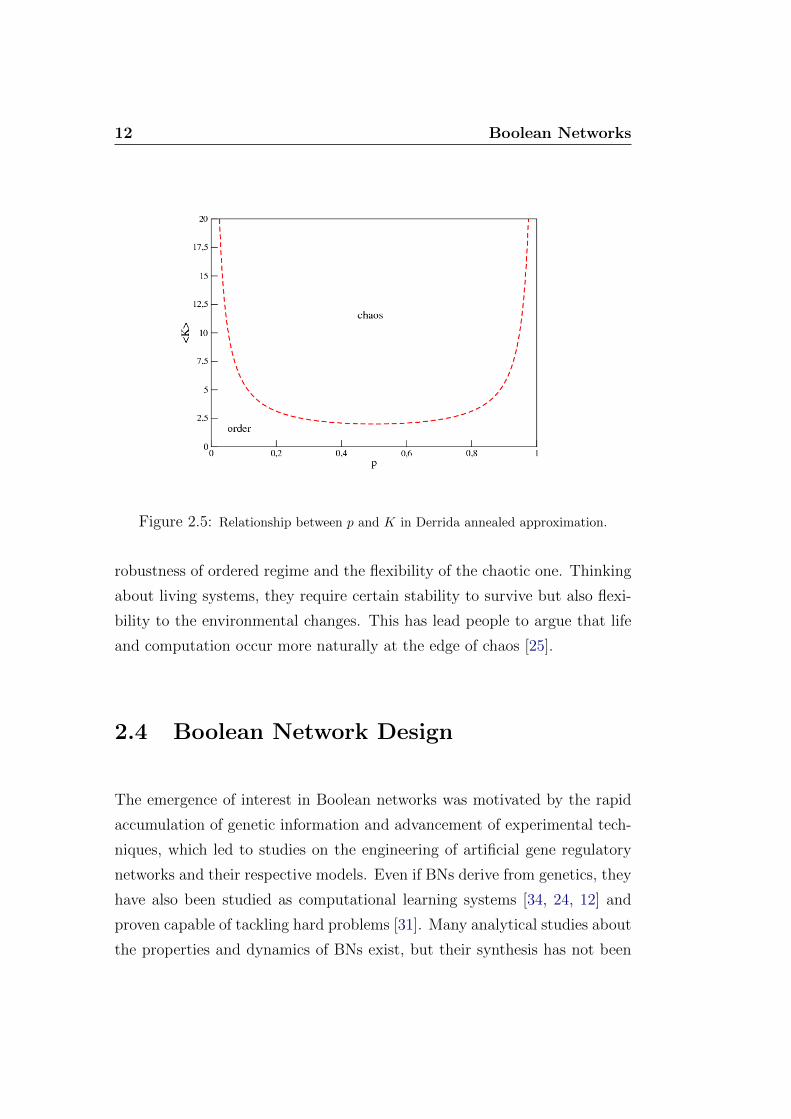
12 Boolean Networks
Figure 2.5: Relationship between p and K in Derrida annealed approximation.
robustness of ordered regime and the flexibility of the chaotic one. Thinking
about living systems, they require certain stability to survive but also flexi-
bility to the environmental changes. This has lead people to argue that life
and computation occur more naturally at the edge of chaos [25].
2.4 Boolean Network Design
The emergence of interest in Boolean networks was motivated by the rapid
accumulation of genetic information and advancement of experimental tech-
niques, which led to studies on the engineering of artificial gene regulatory
networks and their respective models. Even if BNs derive from genetics, they
have also been studied as computational learning systems [34, 24, 12] and
proven capable of tackling hard problems [31]. Many analytical studies about
the properties and dynamics of BNs exist, but their synthesis has not been

2.4 Boolean Network Design 13
deeply studied. The first contribute in this direction is due to Kauffman and
Smith [26] where they proposed some issues that arise in applying Darwin’s
idea to the problem of designing adaptive automata. Subsequently, Lemke
et al. [28] investigate the adaptation of RBNs considering a general genetic
algorithm and a fitness function that takes into account the full network dy-
namical behaviour. Interesting inferences emerge related to the analysis of
the scenario that describes the adaptation on the proposed fitness landscape.
Some studies on the evolvability and robustness are conducted [2, 7, 13].
Szejka and Drossel in [45] focus on networks with canalizing functions where
the evolution is obtained with an adaptive walk. They found that in spite
of having a high degree of robustness, the evolved networks still share many
features with chaotic network. Fretter et al. [16] investigate the propaga-
tion of perturbations in Boolean networks by evaluating the Derrida plot
and modifications of it. They conclude that the simple distinction between
frozen, critical and chaotic networks is no longer useful, since such evolved
networks can display properties of all three types of networks. In addition,
Roli et al. [37] found some differences among the three kinds of networks.
They discuss the results of an experimental analysis in the design of Boolean
networks by means of genetic algorithms. The target of the evolution is to
find a network able to reach an attractor of a specific length. Initial popu-
lations composed of critical or chaotic networks are more likely to reach the
target. Moreover, the evolution starting from critical networks achieves the
best overall performance.

14 Boolean Networks

3. Boolean Networks Robotics
This chapter first introduces the Boolean Network Robotics (Sec. 3.1) pro-
viding some basic concepts useful tu understand the reasons of interest for
this field. After, (Sec. 3.2) it describes in detail the methodology that un-
derlies the automatic design procedure. In Sec. 3.3 we report some recent
works that validate such methodology.
3.1 Basics
The very recent concept of Boolean Networks Robotics refers to the design
of robotic or multi-agent systems. To date, only a few preliminary studies
exist that focus on this problem [40, 18, 3, 39, 41, 38].
As in classical robotics, we consider two principal actors: the agent and
the environment where the agent acts. The agent (in its most general def-
inition) interacts with the environment using sensors and actuators. The
former ones are needed to sense the environment and the latter ones to act
in function of the goals and the sensed environmental information (see Fig.
3.1). A robot is a special kind of agent that operates inside the real world.
One of the hardest problems in the design of a behaviour for a robot is the
unpredictability of the real world, stemming from complex, non-linear phe-
nomena. In general, non-linear systems implies that we can no longer, as
we can with linear systems, decompose the systems into subsystems, solve

16 Boolean Networks Robotics
Figure 3.1: Interaction between agent and environment.
each subsystem individually, and then reassemble them to give the complete
solution [35].
Thus, in real world scenarios, adaptation to constantly changing condi-
tions is often necessary, rendering rule-based strategies likely to fail. Darwin
suggested that adaptation and complexity could evolve by natural selection
acting successively on numerous small, heritable modifications [15]. That
said, the first proposal that Darwinian selection could generate efficient con-
trol systems can be attributed to Alan Turing in the 1950s. He asserted
that intelligent machines capable of adaptation and learning would be too
difficult to conceive by a human designer and could instead be obtained by
using an evolutionary process with mutations and selective reproduction [46].
The idea hinted by Alan Turing has been actually tried in a methodology
called evolutionary robotics. In this approach, genetic regulatory networks
can evolve to obtain the intended behaviour by means of a specific learning
process. BNs are extremely interesting because they are capable of producing
complex behaviours, notwithstanding the compactness of their description.
For this reason, we believe that BNs can effectively play the role of robot
programs [40].

3.2 Methodology 17
3.2 Methodology
The proposed approach consists in using BNs as robot controllers. In this
way, the robot behaviour can be described in terms of trajectories in a state
space, making it possible to design the robot program by directly exploiting
the dynamical characteristics of BNs, such as their attractors, basins of at-
traction and any dynamical property in general. For the design of BN robot,
several interrelated issues have to be tackled.
3.2.1 BN-Robot Coupling
The first issue is called coupling and concerns the mapping between sen-
sors and network inputs and between network outputs and actuators. Many
researchers treat BNs as isolated systems neglecting aspects of interactions
with an external environment. However, some important exceptions exist
[4, 12, 24, 34]. In our case, we divide the network in three specific sets of
nodes: input nodes, hidden nodes and output nodes. The input nodes are
nodes whose state is completely insensitive to the network dynamics (hence
the name) but updated by the sensors readings. Conversely, output nodes
are subjected to the network’s dynamics and their state is observed and used
as signal to trigger or adjust the robot’s actuators. All the remaining nodes
are hidden, i.e., they do not interact with the environment and we conjec-
ture that they could house processes related to memory and reasoning. The
output nodes’ states depend on such hidden nodes. The choice of which
nodes to use as input, output or hidden could be fixed a priori or updated
by means of a learning process. Fig. 3.2 shows the scheme of the coupling
between BN and robot. According to the type of sensor or actuator, the
mapping signal-state/state-signal can be one-to-one or obtained as result of
determined function (e.g., the output could correspond to the moving average
of the state values in time).

18 Boolean Networks Robotics
Figure 3.2: Coupling Between BN and robot.
3.2.2 BN-Controller Design
Once the input and the output mappings are defined, we have two ways
to design the resulting Boolean network. The first way is to design a BN
such that its dynamics satisfy given requirements. For example, in corre-
spondence of attractors with largest basins of attraction the robot exhibit
high-level behaviours and the transitions between attractors would corre-
spond to transitions between behaviours. In this way, the robot is driven
by the dynamics of its Boolean network. The latter possibility consists in
modelling the BN design process as a search problem, in which the goal is
maximising the robot’s performance. These two ways are not alternative and
can be combined. For example, once the basic behaviour is obtained with the
latter approach, we can use the former one in order to improve the robot’s
behaviour [41].
We use a design methodology based on metaheuristics. In fact, the design
of a BN that satisfies given criteria can be modelled as a constrained combina-
torial optimisation problem by properly defining the set of decision variables,
constraints and a evaluation function for reward and punish according to the
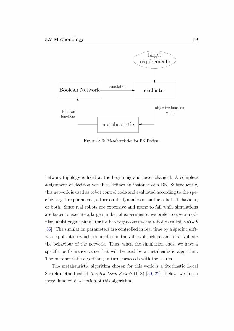
network behaviour. This approach is illustrated by the scheme in Fig. 3.3. In
our work, the decision variables manipulated by the metaheuristic algorithm
correspond to the Boolean functions contained inside the nodes while the
3.2 Methodology 19
Boolean Network
metaheuristic
target
evaluator
Booleanfunctions
objective function
value
simulation
requirements
Figure 3.3: Metaheuristics for BN Design.
network topology is fixed at the beginning and never changed. A complete
assignment of decision variables defines an instance of a BN. Subsequently,
this network is used as robot control code and evaluated according to the spe-
cific target requirements, either on its dynamics or on the robot’s behaviour,
or both. Since real robots are expensive and prone to fail while simulations
are faster to execute a large number of experiments, we prefer to use a mod-
ular, multi-engine simulator for heterogeneous swarm robotics called ARGoS
[36]. The simulation parameters are controlled in real time by a specific soft-
ware application which, in function of the values of such parameters, evaluate
the behaviour of the network. Thus, when the simulation ends, we have a
specific performance value that will be used by a metaheuristic algorithm.
The metaheuristic algorithm, in turn, proceeds with the search.
The metaheuristic algorithm chosen for this work is a Stochastic Local
Search method called Iterated Local Search (ILS) [30, 22]. Below, we find a
more detailed description of this algorithm.
20 Boolean Networks Robotics
3.2.3 Iterated Local Search
As all the stochastic local search algorithms, the Iterated Local Search (ILS)
starts at some location of the search space, representing a possible solution,
and try to improve it by iteratively move from the present location to a neigh-
bouring location. For preventing iterative improvement from getting stuck in
local optima, the ILS essentially alternates two types of search steps: one for
reaching local optima as efficiently as possible, and the other for effectively
escaping from local optima. The landscape that contains these local optima
is defined by an objective function that, in our case, we want to maximize.
Alg. 1 shows an outline for ILS.
Usually, the search process can be initialised in various ways, In this work
we start from a randomly chosen network. For each evaluation, the network
starts from the same randomly chosen state. From this initial candidate so-
lution, a locally optimal solution is obtained by applying a subsidiary local
search procedure localSearch. Subsequently, each iteration of the algorithm
consists of three major stages: perturbation, local search and acceptance crite-
rion. These components need to complement each other for achieving a good
trade-off between intensification and diversification of the search process.
Perturbation a perturbation (perturb) is applied to the current candidate
solution s obtaining a modified candidate solution s′. The role of
perturb is to modify the current candidate solution in a way that will
not be immediately undone by the subsequent local search phase. This
helps the search process to escape from local optima, and the subse-
quent local search phase has more possibility to discover different local
optima. In our case, the perturbation consists in flipping a single bit
randomly chosen into the truth table of each node.
Local Search The next stage is the application of a subsidiary local search
localSearch until a local optimum s′′ is obtained. The local search
procedure has a significant influence on the performance of any ILS
3.2 Methodology 21
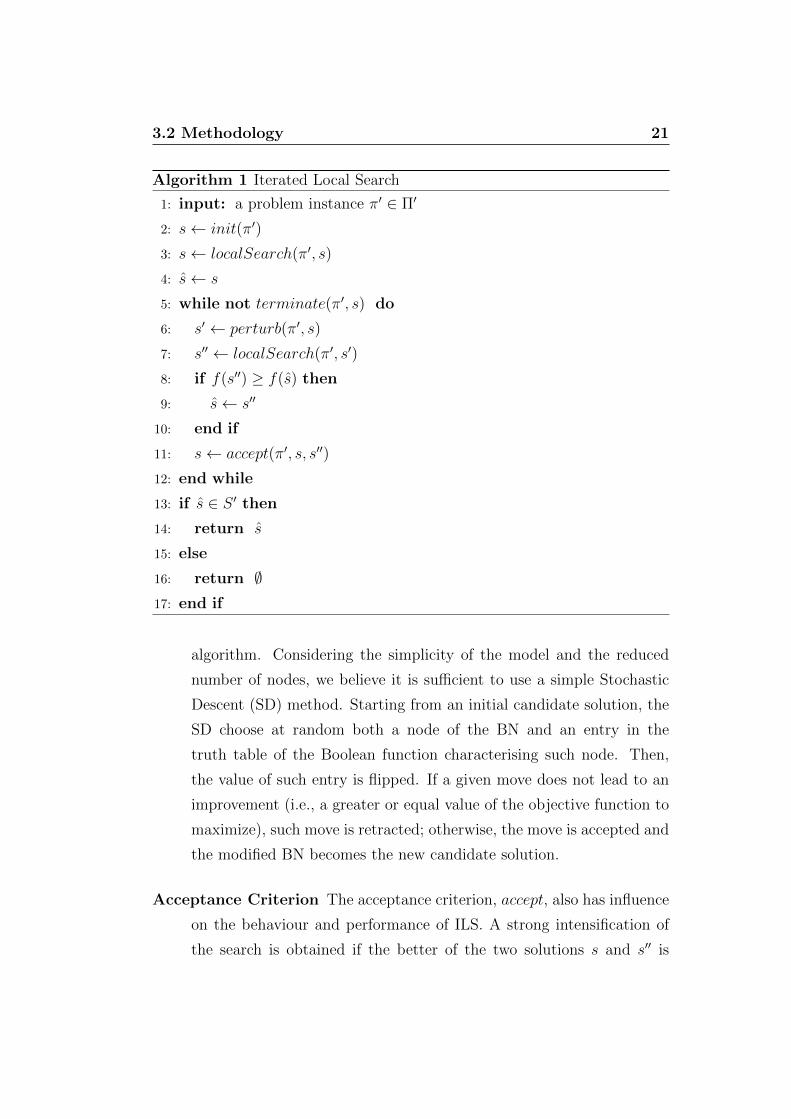
Algorithm 1 Iterated Local Search
1: input: a problem instance π′ ∈ Π′
2: s← init(π′)
3: s← localSearch(π′, s)
4: s← s
5: while not terminate(π′, s) do
6: s′ ← perturb(π′, s)
7: s′′ ← localSearch(π′, s′)
8: if f(s′′) ≥ f(s) then
9: s← s′′
10: end if
11: s← accept(π′, s, s′′)
12: end while
13: if s ∈ S ′ then
14: return s
15: else
16: return ∅17: end if
algorithm. Considering the simplicity of the model and the reduced
number of nodes, we believe it is sufficient to use a simple Stochastic
Descent (SD) method. Starting from an initial candidate solution, the
SD choose at random both a node of the BN and an entry in the
truth table of the Boolean function characterising such node. Then,
the value of such entry is flipped. If a given move does not lead to an
improvement (i.e., a greater or equal value of the objective function to
maximize), such move is retracted; otherwise, the move is accepted and
the modified BN becomes the new candidate solution.
Acceptance Criterion The acceptance criterion, accept, also has influence
on the behaviour and performance of ILS. A strong intensification of
the search is obtained if the better of the two solutions s and s′′ is
22 Boolean Networks Robotics
always accepted. Conversely, if the new local optimum s′′ is always
accepted regardless of its solution quality, the behaviour of the resulting
ILS algorithm corresponds to a random walk in the space of the local
optima of the given evaluation function. For our work, we prefer to
choose s′′ if it is better than or equal to s. Here, for exploring more
of the search space, we accept also a new candidate solution which
performance is the same performance of the previous best solution.
3.3 Related Work
In this work we employed the automatic design methodology seen in Sec. 3.2
in order to synthesize BN-based programs for robots able to perform a given
task. Even though BN robotics is quite recent research field, it is important
to summarise recent work in this area in order to provide its motivations and
perspectives.
Below, we report a summary of the first three works in this direction
where are shown different ways to validate the methodology.
3.3.1 A Proof of Concept
The first contribution in Boolean network robotics comes from Manfroni [40].
In this work, the methodology has been validated by experiments on abstract
case studies (e.g., design of a BN whose trajectory must reach a given a target
state at least once within a certain temporal interval). In these cases, the
networks obtained by automatic design process tend to the critical regime,
that is the most interesting and studied one.
After the validation, the methodology is applied to two robotic tasks:
path following and phototaxis & antiphototaxis. In the former, the robot
selects its actions only on the basis of the current sensory inputs. In the

3.3 Related Work 23
second task, more difficult than the previous one, the robot needs to keep a
sort of internal memory to achieve the goal. The result attained show that
BN dynamics is suitable to produce complex behaviours notwithstanding the
simplicity of the model. However, this work provide only a proof of concept,
without focusing on statistical properties of the methodology, such as its
success rate on robotics case studies.
3.3.2 Improving the Search Method
Garattoni [18] tests the methodology directly on two simple robotic tasks:
phototaxis and obstacle avoidance. The robustness of the methodology is
proven by the good results obtained utilising only a simple stochastic tech-
nique i.e., the stochastic descent. Subsequently, he studies some properties
of the search landscape showing that the dynamical regime of the initial so-
lution can impact the performance of the search process. For instance, initial
solutions in chaotic regime cause a deterioration of the search performance.
Moreover, the choice of the number of nodes can be decisive for the perfor-
mance of the process. In general, a small search landscape make the search
easy, but it is crucial to consider also the required computational capacity for
the target task. Another aspect carried out in that work concerns the link
between the improvements during the training and the network properties.
He shows that relevant improvements in the search landscape correspond to
particular effects on the dynamics of the networks, as the number of states
visited. Finally, the methodology has been employed for a sequence learning
task, more complex due to the form of memory required to be performed. In
this case, the difficulty of the simple stochastic descent emerges in tackling
the task. He proposed different methods with features of search diversifi-
cation, such as the iterated local search and variable neighborhoods search.
From the analysis on the results obtained it is possible to achieve a good
trade-off between intensification and diversification.
24 Boolean Networks Robotics
3.3.3 State Space Analysis
The method is validated also in the work by Amaducci [3], experimenting the
obstacle avoidance and the phototaxis task but the focus of the work is on
the state space structure of the resulting networks. His studies show that the
networks tend to use a low portion of state space to achieve the target task.
In particular, he focuses attention on the relationship between the number
of used states and the quality of results. For example, in the ordered regime,
where the number of used states is lowest, he obtains better results compared
with the chaotic regime in which the number is highest. Furthermore, from
the analysis of the the state distribution during the design process, it emerges
that the number of states is subjected to an exploration phase (i.e., where
the number of visited states increases) and exploitation (i.e., states decrease).
He calls this phenomenom states compression mechanism. The results have
been confirmed with networks of different size. Subsequently, he plots the
entire state space structures showing that the network’s knowledge stored
within the state space is organized in hierarchies that increase the stability
and reliability of the network. From this analysis he states that such large
amount of information can not be extracted just by studying attractors.
The same studies are conducted on the sequence learning task where
the robot is required to keep an internal memory to achieve a given goal.
In this case, he observes a different behaviour in the state space, probably
due to the memory requirements to perform the task. The network realizes
memory by duplicating some portion of its state space and placing it in the
right position of the hierarchy. This mechanism is realized by the states
reuse together with the state space compression and duplication. Finally,
he demonstrates that, independently of the nature of the task, the network
behaviour can be represented by a finite states automaton.
4. Task Description
Starting from the outcomes reached in the previous BN-Robotics works
[40, 18, 3], we now define new objectives to push the limits of this research.
The most important scientific question we want to address is: what happens
inside a system consisting of many BN-controlled robots interacting with each
other? This question is very important, because it moves towards new unex-
plored research areas, such as the interaction among Boolean networks and
new design techniques for swarm robotics. Swarm robotics is an important
application area for swarm intelligence. This concept refers to the emergent
collective intelligence of groups of simple autonomous agents, in particular,
autonomous robots [29]. An autonomous robot is viewed as a system that
acts independently on its environment interacting with other robots around
it. The peculiarity is that an autonomous robot does not follow commands
from a leader [14]. With a swarm of robots we can achieve some tasks that
would be impossible for a single entity.
As we saw in Chapter 3, a methodology exists in order to automatically
design the behaviour of a single robot. The goal of this work is to verify
if such methodology works when applied to a set of interacting robots. In
doing this, we need to define a specific task where collaboration is necessary.
In Sec. 4.1 we introduce the requirements chosen for such task, in Sec. 4.2
we describe in detail all its parts and in Sec. 4.3 we report some similar work
from the field of distributed computation.

26 Task Description
4.1 Task Requirements
The task that we want to consider needs distributed computation and sim-
plicity.
Distributed computation is realized by distributed systems which consist
of multiple autonomous computational entities that communicate through a
network for achieving a common goal. The distributed computation takes
place to solve large computational problems which are too demanding for a
single computational unit. Moreover, the information needed to achieve a
common goal could also be distributed among the nodes of the network. Ac-
cording to the swarm robotics definition, for our task we use a set of robots
with simple computational capabilities. Such robots can only exchange their
limited perceptions with the neighbourhood. The goal is to recognize a cer-
tain environment, whose characteristics can not be fully collected by local
perceptions of a single robot. Here, it is necessary that each robot commu-
nicates its local information until a consensus is reached.
Simplicity is a key issue when, as in our case, we do not have full knowl-
edge of the systems that we want to use. Indeed, although recent studies have
provided the tools to analyze the internal dynamics of Boolean networks, such
systems are yet partially unknown and many aspects are still unexplored. For
this reason, we use simple BN with a small number of nodes. Furthermore,
we employ such networks into simplified environments where the noise com-
ponent does not exist. In these conditions, the computational complexity is
reduced and it is possible to execute a large number of experiments. This
means that we can test the networks on a considerable amount of cases in
order to obtain a complete and thorough picture of the network behaviour.
4.2 Description
The task on which we want to validate the methodology consists of a swarm
of robots that communicate locally among them trying to recognize two dif-
4.2 Description 27
ferent floor patterns. Each robot can only sense the portion of floor below
itself and then send this information into the environment. Each robot, both
transmitter and receiver, perceives the information of the closest robot from
each cardinal point so that is also potentially able to understand what comes
from where (e.g., the northern robot perceives black floor, the southern one
a white floor, etc...). Each robot is equipped with LEDs which can be per-
ceived from an external observer. The goal is to design controllers able to
keep off all the LEDs of the entire swarm if the robots are placed on a certain
floor and turn on all the LEDs whether the swarm is located on the other
one.
Below, we report a more detailed description of the robots used for this
task, in particular the mapping between BN network and controller. Subse-
quently, we report a description of the floor patterns and of different initial
conditions on which we train the network.
4.2.1 Robots
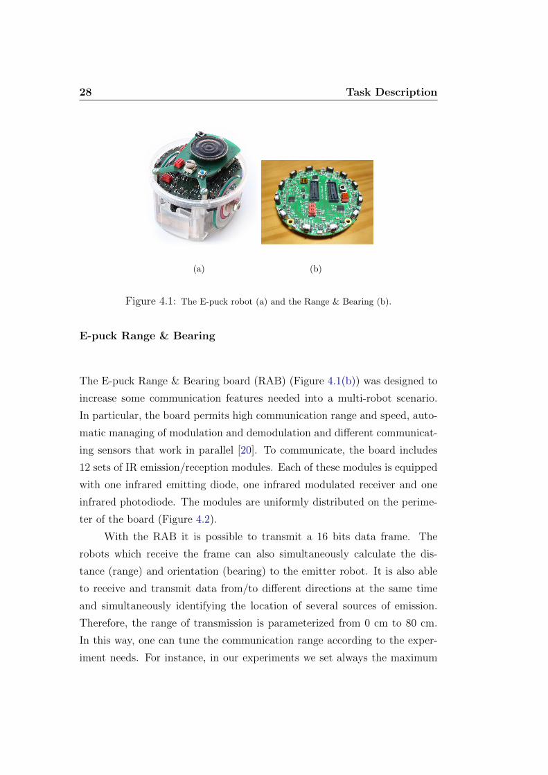
The robot used for our experiments is called E-puck and it is showed in Fig.
4.1(a). The E-puck is a simple robot designed for educational and research
purposes. The full access to knowledge at every level of this robot improves
both the quality of the support to the students and the diffusion in the
research community [33].
A standard E-puck is equipped with several sensors and actuators but
only a small part of them is necessary for our issues. Moreover, we integrate
the robot structure with an open hardware/software board called E-puck
Range & Bearing that enables the robots to communicate and at the same
time obtain the range and bearing of the source of emission. Now we describe
the utilized sensors and actuators.
28 Task Description
(a) (b)
Figure 4.1: The E-puck robot (a) and the Range & Bearing (b).
E-puck Range & Bearing
The E-puck Range & Bearing board (RAB) (Figure 4.1(b)) was designed to
increase some communication features needed into a multi-robot scenario.
In particular, the board permits high communication range and speed, auto-
matic managing of modulation and demodulation and different communicat-
ing sensors that work in parallel [20]. To communicate, the board includes
12 sets of IR emission/reception modules. Each of these modules is equipped
with one infrared emitting diode, one infrared modulated receiver and one
infrared photodiode. The modules are uniformly distributed on the perime-
ter of the board (Figure 4.2).
With the RAB it is possible to transmit a 16 bits data frame. The
robots which receive the frame can also simultaneously calculate the dis-
tance (range) and orientation (bearing) to the emitter robot. It is also able
to receive and transmit data from/to different directions at the same time
and simultaneously identifying the location of several sources of emission.
Therefore, the range of transmission is parameterized from 0 cm to 80 cm.
In this way, one can tune the communication range according to the exper-
iment needs. For instance, in our experiments we set always the maximum

4.2 Description 29
Figure 4.2: (a) Emitters and (b) receivers distribution around the perimeter of the RAB.
range in order to be sure that each robot can sense at least a neighbour.
Ground Sensors
The ground sensors (GS) are composed of three active IR proximity sensors
placed in the front of the e-puck pointing directly at the ground [9]. These
sensor elements are mounted on a small printed circuit board (PCB) which
includes a microcontroller that continually samples the IR sensor elements.
Each IR sensor consists of an IR-emitting diode and a phototransistor. The
IR diode is used to emit a constant amount of infrared beam while the pho-
totransistor detects the amount of signal reflected by the surface. A white
surface reflects much more IR signal than a black surface. The e-puck Ground
Sensors can be used for several different applications. In our case, we employ
the sensor simply to understand whether the surface below the robot is black
or white.
LEDs
The E-puck is equipped by eight red light emitting diodes (LEDs) placed all
around the robot. These LEDs are covered by a translucent plastic and it is
possible to modulate their intensities. In our task, the LEDs are used as a
visual interface for the user to evaluate the correct behaviour of the robot.
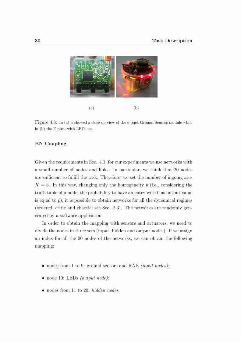
30 Task Description
(a) (b)
Figure 4.3: In (a) is showed a close-up view of the e-puck Ground Sensors module while
in (b) the E-puck with LEDs on.
BN Coupling
Given the requirements in Sec. 4.1, for our experiments we use networks with
a small number of nodes and links. In particular, we think that 20 nodes
are sufficient to fulfill the task. Therefore, we set the number of ingoing arcs
K = 3. In this way, changing only the homogeneity p (i.e., considering the
truth table of a node, the probability to have an entry with 0 as output value
is equal to p), it is possible to obtain networks for all the dynamical regimes
(ordered, critic and chaotic; see Sec. 2.3). The networks are randomly gen-
erated by a software application.
In order to obtain the mapping with sensors and actuators, we need to
divide the nodes in three sets (input, hidden and output nodes). If we assign
an index for all the 20 nodes of the networks, we can obtain the following
mapping:
• nodes from 1 to 9: ground sensors and RAB (input nodes);
• node 10: LEDs (output node);
• nodes from 11 to 20: hidden nodes.
4.2 Description 31
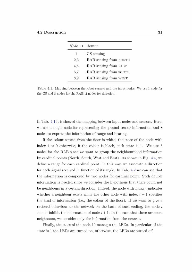
Node id Sensor
1 GS sensing
2,3 RAB sensing from north
4,5 RAB sensing from east
6,7 RAB sensing from south
8,9 RAB sensing from west
Table 4.1: Mapping between the robot sensors and the input nodes. We use 1 node for
the GS and 8 nodes for the RAB: 2 nodes for direction.
In Tab. 4.1 it is showed the mapping between input nodes and sensors. Here,
we use a single node for representing the ground sensor information and 8
nodes to express the information of range and bearing.
If the colour sensed from the floor is white, the state of the node with
index 1 is 0 otherwise, if the colour is black, such state is 1. We use 8
nodes for the RAB since we want to group the neighbourhood information
by cardinal points (North, South, West and East). As shown in Fig. 4.4, we
define a range for each cardinal point. In this way, we associate a direction
for each signal received in function of its angle. In Tab. 4.2 we can see that
the information is composed by two nodes for cardinal point. Such double
information is needed since we consider the hypothesis that there could not
be neighbours in a certain direction. Indeed, the node with index i indicates
whether a neighbour exists while the other node with index i + 1 specifies
the kind of information (i.e., the colour of the floor). If we want to give a
rational behaviour to the network on the basis of such coding, the node i
should inhibit the information of node i+ 1. In the case that there are more
neighbours, we consider only the information from the nearest.
Finally, the state of the node 10 manages the LEDs. In particular, if the
state is 1 the LEDs are turned on, otherwise, the LEDs are turned off.

32 Task Description
34
π −34
π
−π
4π
4
North
South
EastWest
Figure 4.4: E-puck with RAB perceptions by cardinal points. The arrow indicates the
front of the E-puck. The dashed lines identify the range for each cardinal points. According
to the simulator, the angles are in radians increasing in an anticlockwise direction within
the range [−π, π].
4.2.2 Environment
The environments employed for the task are simple bidimensional textures
that define the floors where the robots are placed. As showed in Fig. 4.5,
we use two kinds of floor. The former is a black-white tetromino composed
of four quadrants of alternating colour (like a simplified chessboard) while
the latter is a white floor with a black circle in the centre (like the Japanese
flag).
The chessboard texture is axially symmetrical while the Japanese flag is
also radially symmetric. The presence of such symmetries combined with a
uniform robot distribution prevents the creation of positional bias. Namely,
wherever the robots are placed, we always obtain the same quality of spatial
information.

4.2 Description 33
xi xi+1 Description
0 x no neighbours
1 0 neighbour exists and perceives white
1 1 neighbour exists and perceives black
Table 4.2: Coding of the values for each couple of nodes (xi, xi+1) driven by the RAB.
When the node xi is 0 there is no neighbours.
(a) (b)
Figure 4.5: The patterns chosen for the recognition task. In (a) is showed the chessboard
floor while in (b) the Japanese flag floor.
4.2.3 Initial Conditions
Our goal is to obtain BN controllers that permit to the swarm the recognition
of the floors regardless the position and orientation of the robots. To do that,
a training process that evaluate the network on multiple initial conditions
is necessary. Such initial conditions differ by distribution and orientation.
Indeed, if we evaluate the network on a single distribution, we obtain a too
specialized behaviour that might not work if robots change position. Thus,
the higher the number of initial conditions, the more general the behaviour
of the network obtained at the end of the process.

34 Task Description
Robot Placement
Both the floors have texture composed by only two colours. In order to avoid
bias, we should not prefer an information over the other one i.e., it is impor-
tant to have the same amount of robots placed on both colours.
In order to uniformly distribute the robots, we use the Diffusion Algo-
rithm. Such algorithm simulates the behaviour of gas molecules which, col-
liding with each other, moving and uniformly cover the surrounding environ-
ment. Thus, we realise a simple secondary task where the swarm moves on a
generic arena implementing the diffusion algorithm. The arena has same size
as that defined for the original task. After an initial transient, we sample
periodically the position of each robot. In this way, we obtain a series of
different distributions of robots that we use as different initial conditions for
the evaluation.
4.3 Distributed Computation
From this work, thematics emerge such as self-organization and pattern clas-
sification. We can easily find studies about them in the literature. However,
it does not exist yet a work where such issues are treated for a swarm of
BN-controlled robots. Below, we report an overview of two specific research
areas that, taken together, slightly approach our issues: the sensors networks
and cellular automata.
4.3.1 Sensors Networks
Sensor Network (SN) consist of a large number of cheap, smart devices with
multiple on-board sensors, networked through wireless links and the Internet.
SNs provide unprecedented opportunities for instrumenting and controlling

4.3 Distributed Computation 35
homes, cities, and the environment [10]. Sensor networks may have many
different types of sensors [1] such as seismic, low sampling rate magnetic,
thermal, visual, infrared, acoustic and radar, which are able to monitor a
wide variety of ambient conditions that include:
• temperature,
• humidity,
• vehicular,
• movement,
• lighting condition,
• pressure,
• noise levels,
• the presence or absence of certain kinds of objects,
• mechanical stress levels on attached objects, and the current charac-
teristics such as speed, direction, and size of an object.
In this field, the more interesting issue concerns the extension of the au-
tonomy of the sensors constituting the network. To this end, it is important
to conserve energy and to give up performance in other aspects of the op-
eration such as QoS and bandwidth utilization [43]. Thus, it is crucial to
find a good protocol for exchanging information with a good trade-off among
energy saving and QoS.
A remarkable work is [8] where is deeply described how a SN can solve
the distributed classification problem. They consider the tracking and the
classification of a target that crosses the sensor network. Each object in the
sensor field generates a time-varying spatial signature field that is sensed
36 Task Description
using multiple modalities. The classification is obtained by sampling the tar-
get’s signals over time and analyzing the corresponding time series.
There are two ways to achieve the classification: fusing data or fusing de-
cision. In both cases, there are some master nodes, different from the others,
that collect all data/decision to compute the final result. In general, we can
assert that the SN protocols assign roles to the network’s components. This
aspect is further confirmed in [5] and [10] where they sustain that SNs have
many similarities with multi-agent systems technology.
4.3.2 Cellular Automata
In the field of sensor networks the main issues concern the processing of sig-
nals coming from the real world and the autonomy of the physical devices.
Differently, a cellular automaton (CA) is a decentralized computing theoreti-
cal model principally studied to provide an excellent platform for performing
complex computation with the help of only local information. More pre-
cisely, we have a simple model of a spatially extended (in a certain number
of dimensions) decentralized system made up of a number of individual com-
ponents called cells [17]. The communication between cells is limited to local
interaction. Each individual cell is in a specific state which changes over time
depending on the states of its local neighbours. The overall structure can be
viewed as a parallel processing device. This simple structure when iterated
several times produces complex patterns displaying the potential to simulate
different sophisticated natural phenomena. In order to enable the CA to
reach a given computational goal, the researchers should be able to predict
the global behaviour from the local CA rules. If this was possible, one should
be able to design the local rules/initial conditions from a given prescribed
global behaviour. The only general method to determine the qualitative (av-
erage) dynamics of the system is to run simulations on a computer for various
initial global configurations.

4.3 Distributed Computation 37
The inverse problem of deducing the local rules from a given global be-
haviour is extremely difficult. There have been some efforts, with limited suc-
cess, to build the attractor basin according to a given design specifications.
However, the most popular methodologies to address the inverse problem
of mapping the global behaviour to local CA rules are based on evolution-
ary computation techniques. One of these attempts is [32] where a genetic
algorithm (GA) is used to evolve CAs for two computational tasks: density
classification and synchronization. In both cases, the GA finds rules that give
rise to sophisticated emergent computational strategies. For understanding
how this individual works, they use a general method for reconstructing
the intrinsic computation. This method is called computational mechanics
framework and decomposes the behaviour in regular domains, particles and
particle interactions.
Considering the focus of our work, an interesting study is described in
[42] where the main goal is to understand under which conditions a given set
of interacting Boolean networks can be found in the same attractor. This
work is interesting because each cell is a random Boolean network that shares
some nodes with its neighbourhood. The value of these shared nodes is de-
termined by interaction functions which consider the shared nodes of neigh-
bouring cells. Each cell has the same structure and is driven by the same
interaction function. In these conditions, the CA evolves in discrete time.
Several experiments are launched with different initial condition, number of
shared nodes and different interaction functions. In order to measure the
influence of interaction on the degree of order, they define some variables
as a function of the presence of attractors into the CAs. In this way, it is
possible to classify the CAs in four classes on the basis of their response as
a function of the interaction strength. Moreover, analysing the values of the
variable called average attractor period (AMP) it is possible to understand
which class contains a certain CA. Although the phenomena observed are
complicated, they can provide insights to determine new ways to study the
interaction of random boolean networks.

38 Task Description
5. Preliminary Experiments
In this Chapter we report the sequence of preliminary experiments on which
we have validated the methodology. Sec. 5.1 describes the initial experimen-
tal settings such as the optimisation algorithm, the initial conditions, the
number of iterations and the sets of networks. Section 5.2 shows the results
using a simple stochastic descent method. Sec. 5.3 and Sec. 5.4 report the
experiments using the iterated local search method according two different
objective functions. In Section 5.5 we define a more sophisticated objective
function and we draw some considerations applying it on two cases of output
nodes encoding. Finally, Sec. 5.6 reports the results of experiments setted
by the previous considerations.
5.1 Initial Setting
We have launched 90 experiments with the following configuration:
Number of trials: 30
Iterations: 10000
Number of E-pucks: 20
For each experiment we have 20 E-pucks with the same initial Boolean
network as controller. The networks are generated at random but according
to the following features:

40 Preliminary Experiments
• A total of 20 nodes;
• 9 input nodes: 1 node connected to the ground sensor, 8 nodes con-
nected to the range and bearing sensor;
• 1 output node to set the LEDs ON or OFF;
• Every input node is connected at least to a hidden node;
• Every hidden and output node has 3 ingoing connections (K = 3).
The networks used for the experiments can be grouped in three batches
with different homogeneity p (i.e., considering the truth table of a node, the
probability to have an entry with 0 as output value is equal to p).
• 30 initial networks with p = 0.5
• 30 initial networks with p = 0.788675
• 30 initial networks with p = 0.85
Such homogeneity values statistically correspond to chaotic, critical and
ordered regime (see Sec. 2.3). For each experiment, the robots have the same
network with identical initial state randomly generated.
We call trial a specific initial condition where the swarm of robots will be
simulated and evaluated. For each trial, every E-puck has a given position
and orientation. The criteria for assigning the positions and orientations are
widely described in Sec. 4.2.3. Each step of the training process evaluate
the simulation on 30 trials. In the first fifteen, the robots are placed on a
black-white tetromino floor while in the other ones we have the Japanese flag
floor.
To ensure a correct comparison on the two patterns, we set the same
positions and orientations for both sets of trials (i.e., let N the number of
5.1 Initial Setting 41
trials, the trial 1 has the same robot distribution and orientations of trial
N/2). The only thing that changes is the floor texture.
For each trial, the optimisation algorithm executes the simulation for
10000 times with these parameters:
Length: 20 (simulated seconds)
Ticks per second: 10
Random seed: 312
For the description of the robots’ behaviour during the simulation, you
can trace back to the Section 4.2. Let T the number of the simulation time
steps and x(t)i the behaviour of the epuck i at the time t, we consider the
performance Pn,k of a network n on a certain trial k as the number of correct
behaviours at the last time step t = T (Eq. 5.1).
Pn,k =
∑N
i=1 x(t)i t = T
0 otherwise
, x(t)i =
1 led is correct
0 otherwise(5.1)
Sorting in descending order all the network performances for K trials, we
obtain the distribution DK
DK = {Pn,1, . . . , Pn,K} (5.2)
In this first setting, we define an evaluation function E(1) as the median
value of the distribution DK . The objective function to maximize F (1) is
simply equal to E(1).
E(1) = Pn,K2+1 , F (1) = max E(1) (5.3)
In the section below, we try to optimize the networks using a simple
stochastic descent method (Sec. 3.2.3).
42 Preliminary Experiments
5.2 First Step: Stochastic Descent Results
At first glance, the results are not very satisfactory. In Fig. 5.1 we can see
two graphs. The first one (Fig. 5.1(a)) shows the boxplot of performance
values for each job. Boxplot is a convenient way of graphically depicting
groups of numerical data. The spacings between the different parts of the
box help indicate the degree of dispersion (spread) and skewness in the data.
The bottom and top of the box are always the 25th and 75th percentile (the
lower and upper quartiles, respectively), and the band in the middle of the
box is always the 50th percentile (the median). The ends of the whiskers
can represent several possible alternative values. In our case, the minimum
and maximum of all the data. Any data not included between the whiskers
are plotted as an outlier with a small circle. In this case, we note that the
median value is fairly low (14 on a maximum value of 20) even if some job
gets the value 15.
The second graph (Fig. 5.1(b)) is a histogram of the first iteration with
the best performance value for each job. Here, we can see that most of the
jobs reach the best value before 2000 iterations of the optimisation algorithm.
This suggests that an increase in the number of iterations is not necessary,
but rather, we need a better algorithm.
Finally, in the boxplot of Fig. 5.2 the values are divided by trial and
related to the last iteration with the best value reached. Considering only the
median values, we note that the second pattern (”Japanese flag”) is better
recognized by the swarm and the variance also is smaller.
5.3 Second Step: Iterated Local Search
On the basis of previous results we can conclude that the Stochastic Descent
algorithm is too weak to obtain a satisfactory result. We will try with the
Iterated Local Search algorithm (Sec. 3.2.3) with the Stochastic Descent

5.3 Second Step: Iterated Local Search 43
●
●
●●
●
●●
●
●
1011
1213
1415
Best Value for each job
Obj
Fun
ctio
n
(a)
The first iteration with the best value for each job
Iteration
Fre
quen
cy
0 2000 4000 6000 8000
05
1015
2025
3035
(b)
Figure 5.1: (a) shows the boxplot of the best value of each job. (b) is a histogram that
indicates the frequency of achieving best value as a function of iterations.
logic wrapped inside. In this scenario, we have two levels of perturbation
that we call ILS perturbation and SD perturbation. The SD perturbation
takes place inside the Stochastic Descent algorithm contained within the ILS
body. This perturbation flips a bit of a boolean network’s node chosen at
random. Differently, the ILS perturbation flips a bit chosen at random for
each boolean network node (input nodes excluded). Thus, we launch the
experiments with the parameters below:
Number of trials: 30
Iterations: 20
SD Iterations: 500
Number of E-pucks: 20
Where Iterations and SD Iterations are respectively the iterations of the
ILS algorithm and the iterations of the Stochastic Descent within it. The
total number of SD iterations is 10000; like the previous case.

44 Preliminary Experiments
●
●
●●●
●
●
●
0 2 4 6 8 10 12 14 16 18 20 22 24 26 28
05
1015
20
Values for each trial, for each job
Trial
Eva
luat
ion
Fun
ctio
n
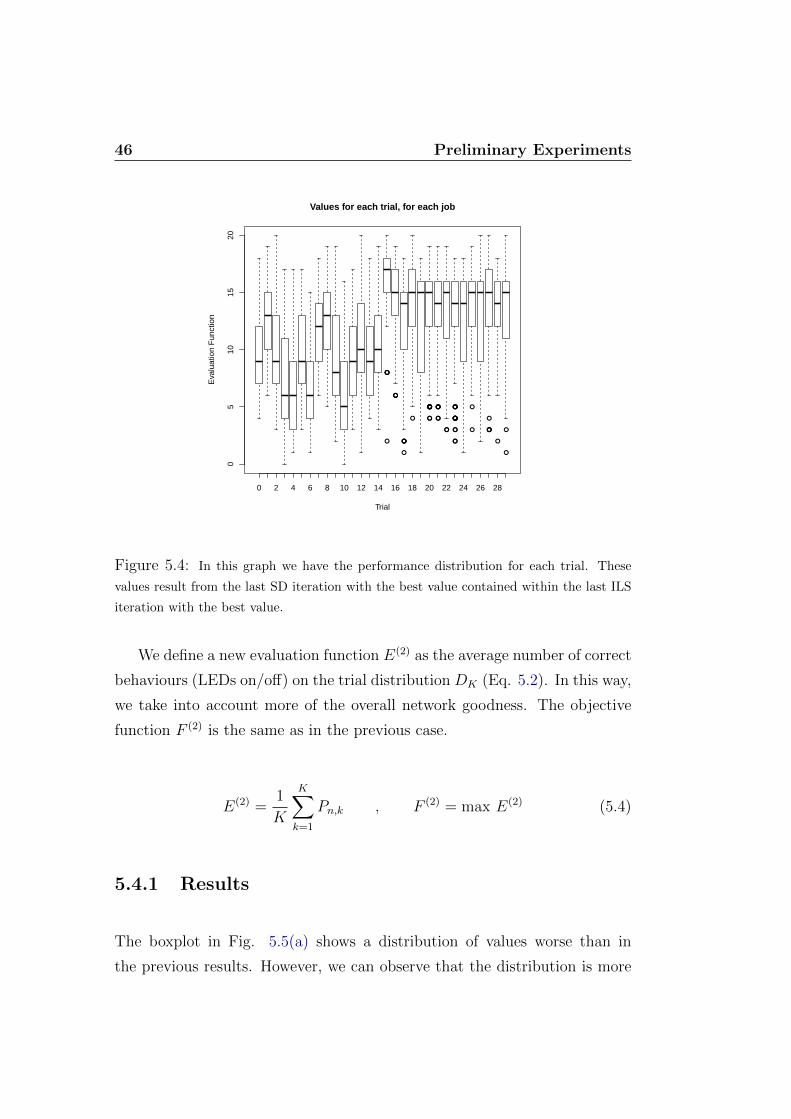
Figure 5.2: In this graph we have the performance distribution for each trial. The first
half of boxplot relates to the chessboard, the second half to the Japanese flag.
5.3.1 Results
By looking at Fig. 5.3(a), a slight improvement could be observed with
respect to the previous algorithm. The boxplot’s shape is the same but we
have a outlier in 16. From Fig. 5.3(b) we have almost the same situation
seen before (most of the job reaches the best value before 1000 SD iterations,
i.e., before the 5th ILS iteration).
The performance values showed in Fig. 5.4 refer to the best SD iteration
contained within the best ILS iteration. In this case, the first half of the
trials (first pattern) has lower average values than the previous case and the
second half values are slightly higher. This is due to the use of a rather
myopic objective function. As saw in Eq. 5.3 , we consider only the median
value from the performance distribution on 30 trials forcing the evolution to
improve only this feature. Since the median provides only discrete values, it

5.4 Third Step: Iterated Local Search with Average as ObjectiveFunction 45
●●
●
●1011
1213
1415
16
Best Value for each job
Obj
Fun
ctio
n
(a)
The first iteration with the best value for each job
Iteration
Fre
quen
cy
0 5 10 15 20
05
1015
2025
3035
(b)
Figure 5.3: (a) shows the boxplot of the best values of each job. (b) shows when the
best performance value is reached. The Iterations-axis refers to the ILS iterations.
seems that it is not a good heuristic search for this problem. Thus, we try
with the average which is continuous and more sensitive to the bound values.
5.4 Third Step: Iterated Local Search with
Average as Objective Function
To face this problem we run another batch of experiments with the same
setting seen before:
Number of trials: 30
Iterations: 20
SD Iterations: 500
Number of E-pucks: 20
46 Preliminary Experiments
●●
●
●
●●●
●
●●●
●
●●
●
●
●
●●●●● ●●
●
●
●
●
●●
●●●
●●
●
●
●
●
●
●
●
●
●
●
●
●
●
●●●
●
●
●
0 2 4 6 8 10 12 14 16 18 20 22 24 26 28
05
1015
20
Values for each trial, for each job
Trial
Eva
luat
ion
Fun
ctio
n
Figure 5.4: In this graph we have the performance distribution for each trial. These
values result from the last SD iteration with the best value contained within the last ILS
iteration with the best value.
We define a new evaluation function E(2) as the average number of correct
behaviours (LEDs on/off) on the trial distribution DK (Eq. 5.2). In this way,
we take into account more of the overall network goodness. The objective
function F (2) is the same as in the previous case.
E(2) =1
K
K∑k=1
Pn,k , F (2) = max E(2) (5.4)
5.4.1 Results
The boxplot in Fig. 5.5(a) shows a distribution of values worse than in
the previous results. However, we can observe that the distribution is more

5.5 Fourth Step: Objective Function H 47
●1011
1213
14
Best Value for each job
Obj
Fun
ctio
n
(a)
The first iteration with the best value for each job
IterationF
requ
ency
0 5 10 15 20
02
46
810
(b)
Figure 5.5: The boxplot in (a) shows worse results than previous case while in (b) is
possible to see a landscape with many flourishing areas.
compact. Also in Fig. 5.6 is showed that.
An interesting observation comes from Fig. 5.5(b).The histogram shows
that there is a non negligible fraction of experiments which attain the best
value at 10-15 iterations of ILS. ILS exploits most of the available iterations.
We could then conclude that the objective function E(2) enables the search
process to perform a wider exploration than in the previous cases.
5.5 Fourth Step: Objective Function H
Till this moment, the evaluation has taken place only at the last time step
(see Eq. 5.1). By analysing the simulation, we observe that a cyclical LEDs
behaviour emerges. This makes us conjecture that an evaluation based on
a single time step can be rather noisy. Indeed, the behaviour at the last
considered time step can be completely different from the other nearby steps.
48 Preliminary Experiments
●
●
●
●
●
●
● ●
● ●
●
●●
●
●
●
●
●
●
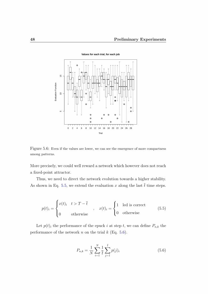
●
●
0 2 4 6 8 10 12 14 16 18 20 22 24 26 28
510
15
Values for each trial, for each job
Trial
Eva
luat
ion
Fun
ctio
n
Figure 5.6: Even if the values are lower, we can see the emergence of more compactness
among patterns.
More precisely, we could well reward a network which however does not reach
a fixed-point attractor.
Thus, we need to direct the network evolution towards a higher stability.
As shown in Eq. 5.5, we extend the evaluation x along the last t time steps.
p(t)i =
x(t)i t > T − t
0 otherwise
, x(t)i =
1 led is correct
0 otherwise(5.5)
Let p(t)i the performance of the epuck i at step t, we can define Pn,k the
performance of the network n on the trial k (Eq. 5.6).
Pn,k =1
N
N∑i=1
1
t
t∑j=1
p(j)i (5.6)
5.5 Fourth Step: Objective Function H 49
Where N is the number of robots and t is the time window length. The
result is normalized according to N . In this way, the networks’ score will be
as high as the number of correct behaviours maintained over t by each robot.
Let DK the sorted (in descending order) performance distribution seen in
Eq. 5.2, we define E the evaluation function on the distribution DK . In Eq.
5.7, we summarise two possibilities tried in the previous steps.
E(1) = Pn,K2+1 , E(2) =
1
K
K∑k=1
Pn,k (5.7)
In this level of evaluation we can add a compactness function c to reward
the networks with smaller variance on the distribution.
c =1
K
K∑k=1
[maxDK
−Pn,k
](5.8)
Here, we calculate the average distance from the maximum value of the
distribution DK normalised on the number of trials K. In order to combine
this function, which is to be maximised, with the previous ones, which is to
be minimised, we introduce a variant, called C (Eq. 5.9).
C = 1− 1
K
K∑k=1
[maxDK
−Pn,k
](5.9)
The combined objective function H is defined as follows:
H = max (αE + (1− α)C) α ∈ [0, 1] (5.10)
The scalar α make it possible to modify the weights of the evaluation
during the training process. For instance, in the first half of the process we
could prefer the definition of networks with good performance and only in the
second half we could tune α in order to increase the importance of compact
results.

50 Preliminary Experiments
5.5.1 Two Different Batches of Experiments
This time we launch two new batches of 90 experiments with the Iterated
Local Search algorithm. Both batches have E(2) as evaluation function (the
average value on the distribution). Furthermore, we try to increase the num-
ber of ILS iteration to enable a larger exploration of the landscape. Below
the setting in detail:
Number of trials: 30
Iterations: 30
SD Iterations: 500
Number of E-pucks: 20
Objective Function: H , (E = E(2), α = 0.8)
For the moment, we maintain the same value for α in all the ILS iterations.
The only difference between the two batches is the epuck’s LEDs actuator.
In the first batch, like the previous cases, the LEDs are directly controlled by
the BN output nodes for each step. In the second one, in order to obtain a
binary value for the LEDs state, we compare the moving average (MA) of the
output node’s value over time with a threshold. We consider values inside a
time window no larger than 9 time steps (Alg. 2). This method permit us
to reduce the network’s oscillation and we move further to the stability.
As shown in Alg. 2 the output node’s state at step j (sj) is always 0 or
1. So, when the value of MA is greater than 0.5 it means that the amount
of 1-values into the buffer S is greater than the 0-values (vice versa with
MA < 0.5 ). When MA = 0.5 we have the same amount of 1s and 0s. In
this case, we choose at random the value for the LEDs.
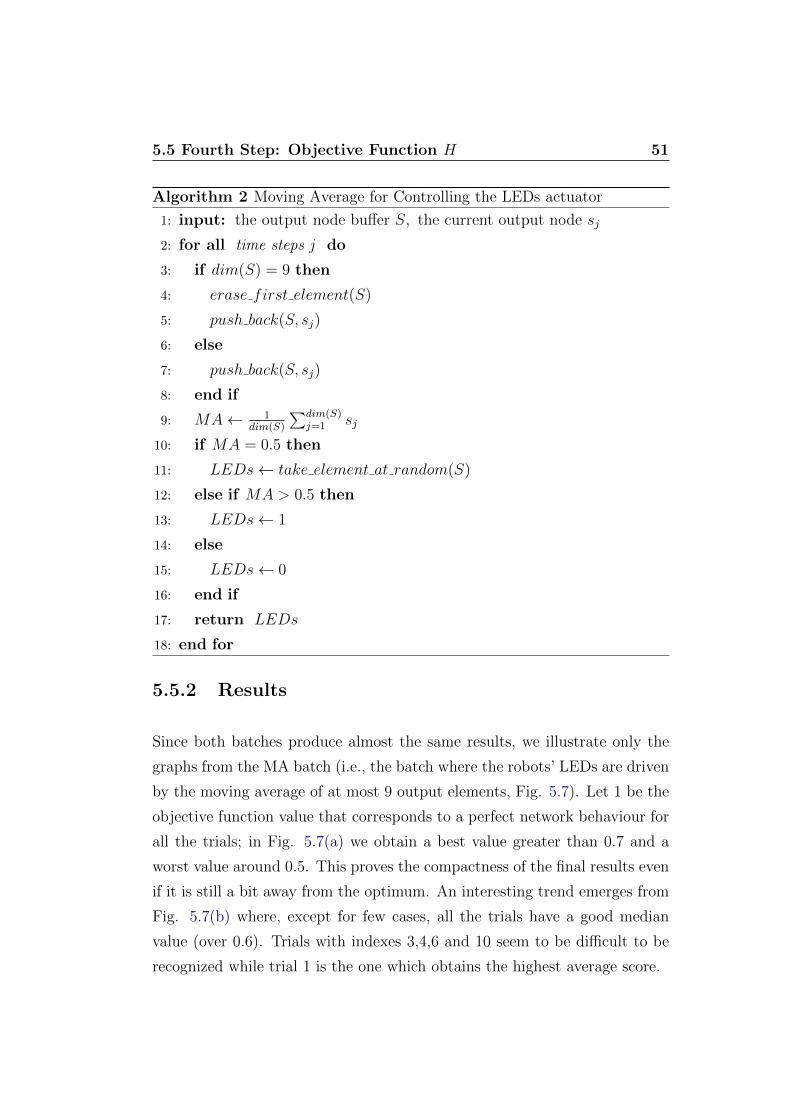
5.5 Fourth Step: Objective Function H 51
Algorithm 2 Moving Average for Controlling the LEDs actuator
1: input: the output node buffer S, the current output node sj
2: for all time steps j do
3: if dim(S) = 9 then
4: erase first element(S)
5: push back(S, sj)
6: else
7: push back(S, sj)
8: end if
9: MA← 1dim(S)
∑dim(S)j=1 sj
10: if MA = 0.5 then
11: LEDs← take element at random(S)
12: else if MA > 0.5 then
13: LEDs← 1
14: else
15: LEDs← 0
16: end if
17: return LEDs
18: end for
5.5.2 Results
Since both batches produce almost the same results, we illustrate only the
graphs from the MA batch (i.e., the batch where the robots’ LEDs are driven
by the moving average of at most 9 output elements, Fig. 5.7). Let 1 be the
objective function value that corresponds to a perfect network behaviour for
all the trials; in Fig. 5.7(a) we obtain a best value greater than 0.7 and a
worst value around 0.5. This proves the compactness of the final results even
if it is still a bit away from the optimum. An interesting trend emerges from
Fig. 5.7(b) where, except for few cases, all the trials have a good median
value (over 0.6). Trials with indexes 3,4,6 and 10 seem to be difficult to be
recognized while trial 1 is the one which obtains the highest average score.
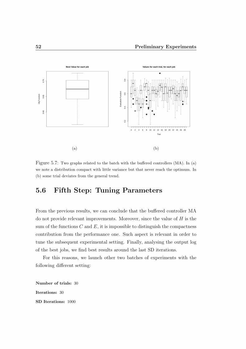
52 Preliminary Experiments0.
600.
650.
70
Best Value for each job
Obj
Fun
ctio
n
(a)
●
●
●
●
●
●
●●●
●
●
●●●
●
●
●●●
●
●
●●●
●●●●●
●●●
●●●
●●●
●●
●
0 2 4 6 8 10 12 14 16 18 20 22 24 26 28
0.2
0.4
0.6
0.8
Values for each trial, for each job
Trial
Eva
luat
ion
Fun
ctio
n
(b)
Figure 5.7: Two graphs related to the batch with the buffered controllers (MA). In (a)
we note a distribution compact with little variance but that never reach the optimum. In
(b) some trial deviates from the general trend.
5.6 Fifth Step: Tuning Parameters
From the previous results, we can conclude that the buffered controller MA
do not provide relevant improvements. Moreover, since the value of H is the
sum of the functions C and E, it is impossible to distinguish the compactness
contribution from the performance one. Such aspect is relevant in order to
tune the subsequent experimental setting. Finally, analysing the output log
of the best jobs, we find best results around the last SD iterations.
For this reasons, we launch other two batches of experiments with the
following different setting:
Number of trials: 30
Iterations: 30
SD Iterations: 1000

5.6 Fifth Step: Tuning Parameters 53
Number of E-pucks: 20
Objective Function: H , (E = E(2), α = 1(batch1), α = 0.9(batch2))
We have increased the number of SD iteration giving more chances to
exploitation. The α value changes in relation to the case. In the former
batch (α = 1) we completely stamp out the C function’s effects (see Eq.
5.10) while we have a weakly presence in the latter (α = 0.9). In this way, it
is possible to prefer the correct behaviour of the robot over the compactness.
Therefore, we want to exclude the ordered networks (i.e., since K is always
3, we exclude the networks with p = 0.85, see Fig. 2.5) and so we launch
only 60 experiments per batch instead of the previous 90. Indeed, because
of their strong resistance to perturbations, the ordered networks are harder
to change than the other ones. Thus, we can save computational time by
focusing only on chaotic and critic networks.
5.6.1 Results
The results are very similar to the previous case. The only difference is
shown in Fig. 5.8 where the median value in the case with α = 1 is under
the threshold of 0.65 while it is slightly above in the other case. We note
that the variance is identical. We think that the greater previous best value
of H (about 0.7) was pushed up by function C. The only influence of E is
not sufficient to improve the results nor with 1000 SD iterations. The other
graphs do not provide any additional information.

54 Preliminary Experiments
0.50
0.55
0.60
0.65
0.70
Best Value for each job
Obj
Fun
ctio
n
(a) best values with α = 1
0.55
0.60
0.65
0.70
Best Value for each job
Obj
Fun
ctio
n
(b) best values with α = 0.9
Figure 5.8: Boxplots of the best values with different influence of E. In both graphs
there are no improvements compared to the previous case.
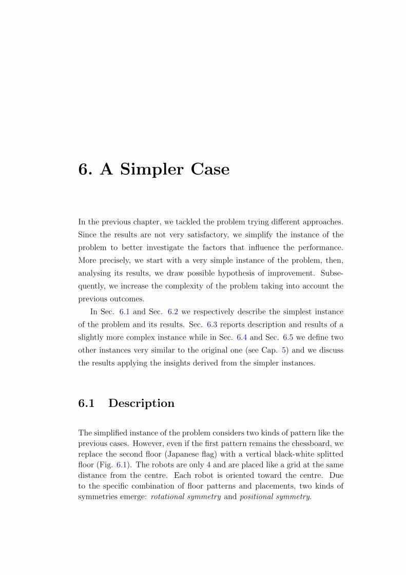
6. A Simpler Case
In the previous chapter, we tackled the problem trying different approaches.
Since the results are not very satisfactory, we simplify the instance of the
problem to better investigate the factors that influence the performance.
More precisely, we start with a very simple instance of the problem, then,
analysing its results, we draw possible hypothesis of improvement. Subse-
quently, we increase the complexity of the problem taking into account the
previous outcomes.
In Sec. 6.1 and Sec. 6.2 we respectively describe the simplest instance
of the problem and its results. Sec. 6.3 reports description and results of a
slightly more complex instance while in Sec. 6.4 and Sec. 6.5 we define two
other instances very similar to the original one (see Cap. 5) and we discuss
the results applying the insights derived from the simpler instances.
6.1 Description
The simplified instance of the problem considers two kinds of pattern like the
previous cases. However, even if the first pattern remains the chessboard, we
replace the second floor (Japanese flag) with a vertical black-white splitted
floor (Fig. 6.1). The robots are only 4 and are placed like a grid at the same
distance from the centre. Each robot is oriented toward the centre. Due
to the specific combination of floor patterns and placements, two kinds of
symmetries emerge: rotational symmetry and positional symmetry.
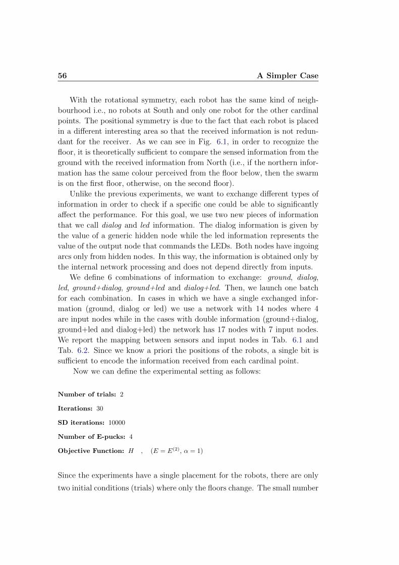
56 A Simpler Case
With the rotational symmetry, each robot has the same kind of neigh-
bourhood i.e., no robots at South and only one robot for the other cardinal
points. The positional symmetry is due to the fact that each robot is placed
in a different interesting area so that the received information is not redun-
dant for the receiver. As we can see in Fig. 6.1, in order to recognize the
floor, it is theoretically sufficient to compare the sensed information from the
ground with the received information from North (i.e., if the northern infor-
mation has the same colour perceived from the floor below, then the swarm
is on the first floor, otherwise, on the second floor).
Unlike the previous experiments, we want to exchange different types of
information in order to check if a specific one could be able to significantly
affect the performance. For this goal, we use two new pieces of information
that we call dialog and led information. The dialog information is given by
the value of a generic hidden node while the led information represents the
value of the output node that commands the LEDs. Both nodes have ingoing
arcs only from hidden nodes. In this way, the information is obtained only by
the internal network processing and does not depend directly from inputs.
We define 6 combinations of information to exchange: ground, dialog,
led, ground+dialog, ground+led and dialog+led. Then, we launch one batch
for each combination. In cases in which we have a single exchanged infor-
mation (ground, dialog or led) we use a network with 14 nodes where 4
are input nodes while in the cases with double information (ground+dialog,
ground+led and dialog+led) the network has 17 nodes with 7 input nodes.
We report the mapping between sensors and input nodes in Tab. 6.1 and
Tab. 6.2. Since we know a priori the positions of the robots, a single bit is
sufficient to encode the information received from each cardinal point.
Now we can define the experimental setting as follows:
Number of trials: 2
Iterations: 30
SD iterations: 10000
Number of E-pucks: 4
Objective Function: H , (E = E(2), α = 1)
Since the experiments have a single placement for the robots, there are only
two initial conditions (trials) where only the floors change. The small number
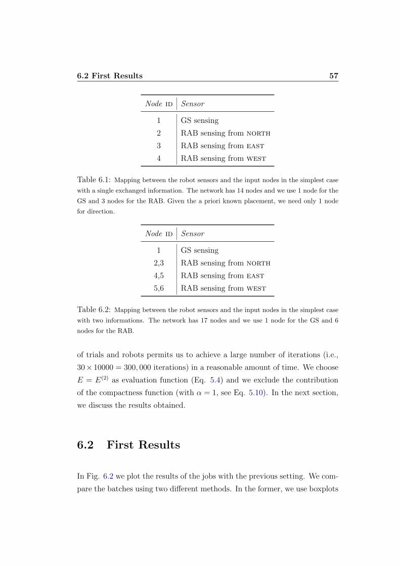
6.2 First Results 57
Node id Sensor
1 GS sensing
2 RAB sensing from north
3 RAB sensing from east
4 RAB sensing from west
Table 6.1: Mapping between the robot sensors and the input nodes in the simplest case
with a single exchanged information. The network has 14 nodes and we use 1 node for the
GS and 3 nodes for the RAB. Given the a priori known placement, we need only 1 node
for direction.
Node id Sensor
1 GS sensing
2,3 RAB sensing from north
4,5 RAB sensing from east
5,6 RAB sensing from west
Table 6.2: Mapping between the robot sensors and the input nodes in the simplest case
with two informations. The network has 17 nodes and we use 1 node for the GS and 6
nodes for the RAB.
of trials and robots permits us to achieve a large number of iterations (i.e.,
30× 10000 = 300, 000 iterations) in a reasonable amount of time. We choose
E = E(2) as evaluation function (Eq. 5.4) and we exclude the contribution
of the compactness function (with α = 1, see Eq. 5.10). In the next section,
we discuss the results obtained.
6.2 First Results
In Fig. 6.2 we plot the results of the jobs with the previous setting. We com-
pare the batches using two different methods. In the former, we use boxplots
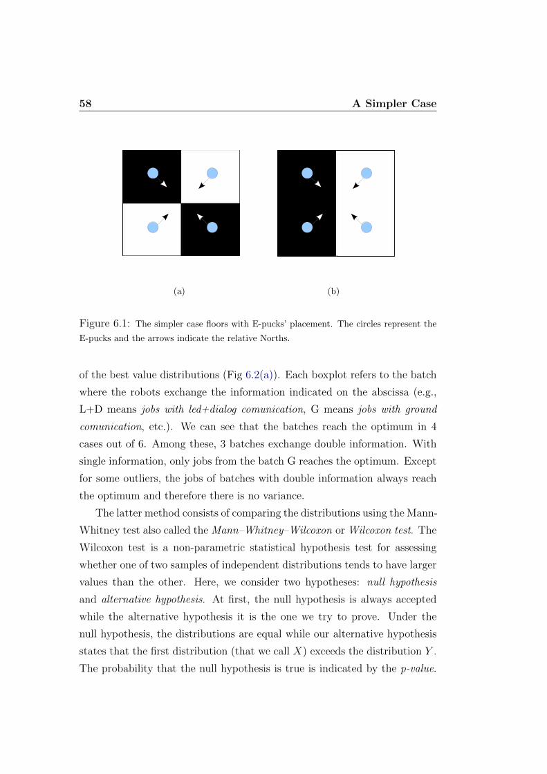
58 A Simpler Case
(a) (b)
Figure 6.1: The simpler case floors with E-pucks’ placement. The circles represent the
E-pucks and the arrows indicate the relative Norths.
of the best value distributions (Fig 6.2(a)). Each boxplot refers to the batch
where the robots exchange the information indicated on the abscissa (e.g.,
L+D means jobs with led+dialog comunication, G means jobs with ground
comunication, etc.). We can see that the batches reach the optimum in 4
cases out of 6. Among these, 3 batches exchange double information. With
single information, only jobs from the batch G reaches the optimum. Except
for some outliers, the jobs of batches with double information always reach
the optimum and therefore there is no variance.
The latter method consists of comparing the distributions using the Mann-
Whitney test also called the Mann–Whitney–Wilcoxon or Wilcoxon test. The
Wilcoxon test is a non-parametric statistical hypothesis test for assessing
whether one of two samples of independent distributions tends to have larger
values than the other. Here, we consider two hypotheses: null hypothesis
and alternative hypothesis. At first, the null hypothesis is always accepted
while the alternative hypothesis it is the one we try to prove. Under the
null hypothesis, the distributions are equal while our alternative hypothesis
states that the first distribution (that we call X) exceeds the distribution Y .
The probability that the null hypothesis is true is indicated by the p-value.
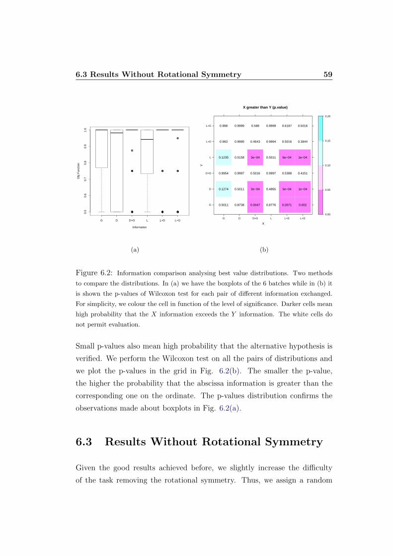
6.3 Results Without Rotational Symmetry 59
●
●
●
●
●
●●●●●● ●
●
●●
●
●●●●●●
●
●
●
●●●●●●
●
G D D+G L L+D L+G
0.5
0.6
0.7
0.8
0.9
1.0
Information
Obj
Fun
ctio
n
(a)
X greater than Y (p.value)
X
YG
D
D+G
L
L+D
L+G
G D D+G L L+D L+G
0.5011 0.8738 0.0047 0.8776 0.0071 0.002
0.1274 0.5011 3e−04 0.4865 5e−04 1e−04
0.9954 0.9997 0.5016 0.9997 0.5388 0.4151
0.1235 0.5158 3e−04 0.5011 6e−04 1e−04
0.993 0.9995 0.4643 0.9994 0.5016 0.3844
0.998 0.9999 0.588 0.9999 0.6187 0.5016
0.00
0.05
0.10
0.15
0.20
(b)
Figure 6.2: Information comparison analysing best value distributions. Two methods
to compare the distributions. In (a) we have the boxplots of the 6 batches while in (b) it
is shown the p-values of Wilcoxon test for each pair of different information exchanged.
For simplicity, we colour the cell in function of the level of significance. Darker cells mean
high probability that the X information exceeds the Y information. The white cells do
not permit evaluation.
Small p-values also mean high probability that the alternative hypothesis is
verified. We perform the Wilcoxon test on all the pairs of distributions and
we plot the p-values in the grid in Fig. 6.2(b). The smaller the p-value,
the higher the probability that the abscissa information is greater than the
corresponding one on the ordinate. The p-values distribution confirms the
observations made about boxplots in Fig. 6.2(a).
6.3 Results Without Rotational Symmetry
Given the good results achieved before, we slightly increase the difficulty
of the task removing the rotational symmetry. Thus, we assign a random
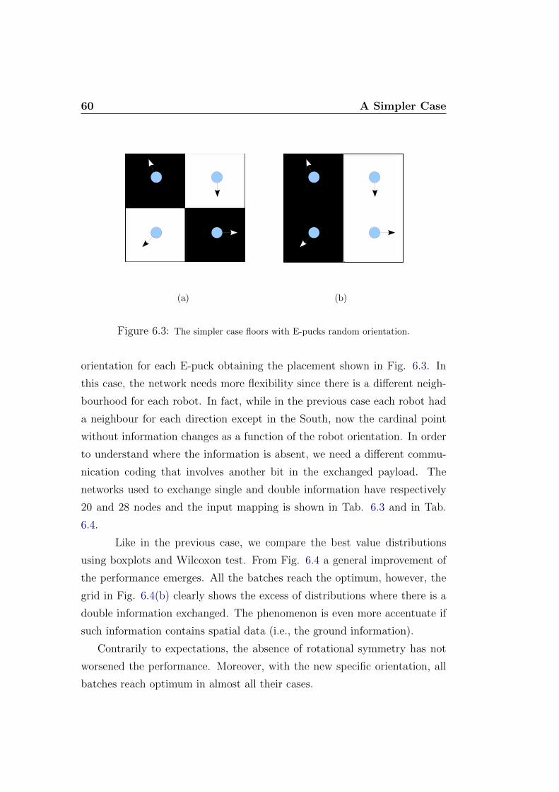
60 A Simpler Case
(a) (b)
Figure 6.3: The simpler case floors with E-pucks random orientation.
orientation for each E-puck obtaining the placement shown in Fig. 6.3. In
this case, the network needs more flexibility since there is a different neigh-
bourhood for each robot. In fact, while in the previous case each robot had
a neighbour for each direction except in the South, now the cardinal point
without information changes as a function of the robot orientation. In order
to understand where the information is absent, we need a different commu-
nication coding that involves another bit in the exchanged payload. The
networks used to exchange single and double information have respectively
20 and 28 nodes and the input mapping is shown in Tab. 6.3 and in Tab.
6.4.
Like in the previous case, we compare the best value distributions
using boxplots and Wilcoxon test. From Fig. 6.4 a general improvement of
the performance emerges. All the batches reach the optimum, however, the
grid in Fig. 6.4(b) clearly shows the excess of distributions where there is a
double information exchanged. The phenomenon is even more accentuate if
such information contains spatial data (i.e., the ground information).
Contrarily to expectations, the absence of rotational symmetry has not
worsened the performance. Moreover, with the new specific orientation, all
batches reach optimum in almost all their cases.
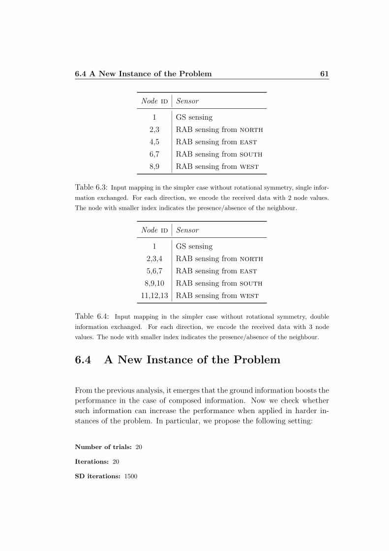
6.4 A New Instance of the Problem 61
Node id Sensor
1 GS sensing
2,3 RAB sensing from north
4,5 RAB sensing from east
6,7 RAB sensing from south
8,9 RAB sensing from west
Table 6.3: Input mapping in the simpler case without rotational symmetry, single infor-
mation exchanged. For each direction, we encode the received data with 2 node values.
The node with smaller index indicates the presence/absence of the neighbour.
Node id Sensor
1 GS sensing
2,3,4 RAB sensing from north
5,6,7 RAB sensing from east
8,9,10 RAB sensing from south
11,12,13 RAB sensing from west
Table 6.4: Input mapping in the simpler case without rotational symmetry, double
information exchanged. For each direction, we encode the received data with 3 node
values. The node with smaller index indicates the presence/absence of the neighbour.
6.4 A New Instance of the Problem
From the previous analysis, it emerges that the ground information boosts the
performance in the case of composed information. Now we check whether
such information can increase the performance when applied in harder in-
stances of the problem. In particular, we propose the following setting:
Number of trials: 20
Iterations: 20
SD iterations: 1500

62 A Simpler Case
●
●●
●
●
●●
●●●●●●●
●●
●●●●●●● ●●●●●●
●
●●●
●
●
●●●●●●●●● ●●●●●●●●●●●●●●●●●
●●
G D D+G L L+D L+G
0.5
0.6
0.7
0.8
0.9
1.0
Information
Obj
Fun
ctio
n
(a)
X greater than Y (p.value)
X
Y
G
D
D+G
L
L+D
L+G
G D D+G L L+D L+G
0.5013 0.9885 0.0036 0.9992 0.9936 0.0422
0.0117 0.5009 0 0.8164 0.6064 2e−04
0.9965 1 1 1 1 0.9231
9e−04 0.1848 0 0.5008 0.2673 0
0.0065 0.3953 0 0.7341 0.5009 1e−04
0.9585 0.9998 0.0792 1 0.9999 0.5023
0.00
0.05
0.10
0.15
0.20
(b)
Figure 6.4: Comparison among best values in the case without rotational symmetry. All
the batches reach the optimum and the best combinations contain the ground information.
Number of E-pucks: 10
Objective Function: H , (E = E(2), α = 1)
Here, the key change is the increase of initial conditions (trials) and robots.
For each trial, we uniformly distribute 10 robots (applying the method de-
scribed in Sec. 4.2.3) and we choose at random the orientations. For com-
putational load issues, we must strongly decrease the number of stochastic
descent iterations (i.e., from 10000 to 1500). The floor patterns remain the
same. In Fig. 6.5 we report the comparison. Although no batch reaches the
optimum, we mostly get a success rate around 80%. The Wilcoxon grid in
Fig. 6.5(b) shows the dominance of “D+G” (dialog+ground) and “L+G”
(led+ground) distribution. Such result is consistent with the simpler case,
confirming the influence of informations composed with spatial data.
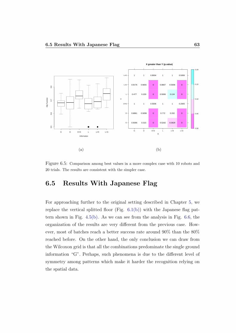
6.5 Results With Japanese Flag 63
●●●●●●●●●●●●●●●●● ●●●●●●●●●●●●●●●●●
G D D+G L L+D L+G
0.5
0.6
0.7
0.8
Information
Obj
Fun
ctio
n
(a)
X greater than Y (p.value)
X
YG
D
D+G
L
L+D
L+G
G D D+G L L+D L+G
0.5006 0.315 0 0.5242 0.0829 0
0.6861 0.5006 0 0.772 0.332 0
1 1 0.5006 1 1 0.2005
0.477 0.229 0 0.5006 0.134 0
0.9176 0.6691 0 0.8667 0.5006 0
1 1 0.8004 1 1 0.5006
0.00
0.05
0.10
0.15
0.20
(b)
Figure 6.5: Comparison among best values in a more complex case with 10 robots and
20 trials. The results are consistent with the simpler case.
6.5 Results With Japanese Flag
For approaching further to the original setting described in Chapter 5, we
replace the vertical splitted floor (Fig. 6.1(b)) with the Japanese flag pat-
tern shown in Fig. 4.5(b). As we can see from the analysis in Fig. 6.6, the
organization of the results are very different from the previous case. How-
ever, most of batches reach a better success rate around 90% than the 80%
reached before. On the other hand, the only conclusion we can draw from
the Wilcoxon grid is that all the combinations predominate the single ground
information “G”. Perhaps, such phenomena is due to the different level of
symmetry among patterns which make it harder the recognition relying on
the spatial data.
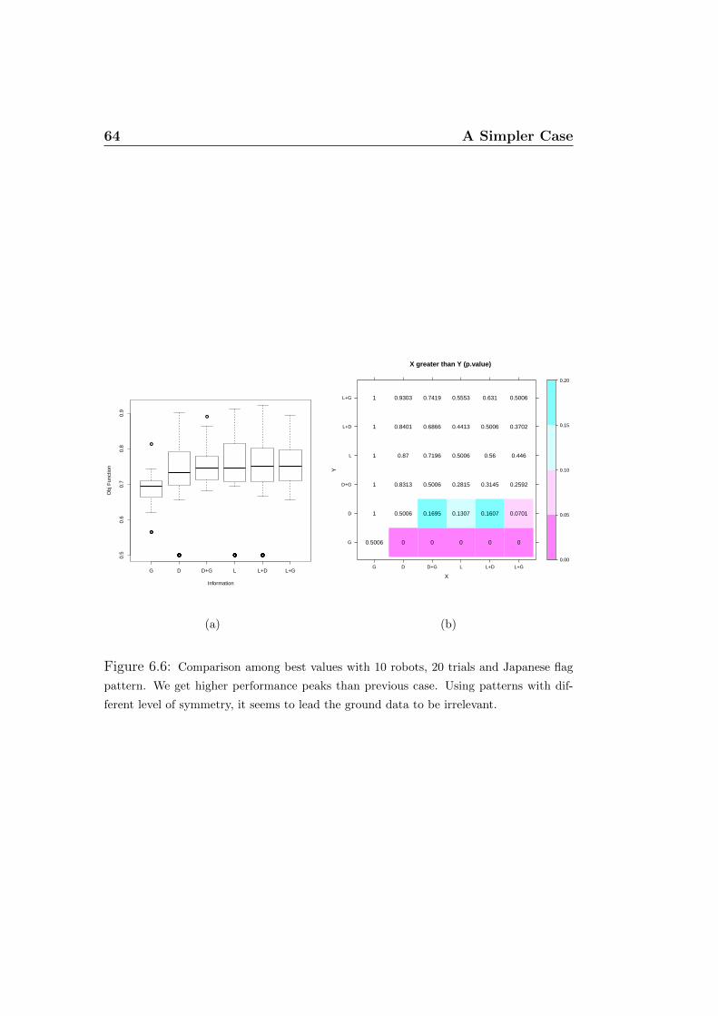
64 A Simpler Case
●●
●
●●●●●●●●●●●●●●
●
●●●●●●●●●●●●●●●●●● ●●●●●●●●●●●●●●●●●
G D D+G L L+D L+G
0.5
0.6
0.7
0.8
0.9
Information
Obj
Fun
ctio
n
(a)
X greater than Y (p.value)
X
Y
G
D
D+G
L
L+D
L+G
G D D+G L L+D L+G
0.5006 0 0 0 0 0
1 0.5006 0.1695 0.1307 0.1607 0.0701
1 0.8313 0.5006 0.2815 0.3145 0.2592
1 0.87 0.7196 0.5006 0.56 0.446
1 0.8401 0.6866 0.4413 0.5006 0.3702
1 0.9303 0.7419 0.5553 0.631 0.5006
0.00
0.05
0.10
0.15
0.20
(b)
Figure 6.6: Comparison among best values with 10 robots, 20 trials and Japanese flag
pattern. We get higher performance peaks than previous case. Using patterns with dif-
ferent level of symmetry, it seems to lead the ground data to be irrelevant.

7. Conclusion
In this thesis we employed an automatic design methodology in order to de-
velop robotic programs for tasks that require collective computation. Such
procedures need two main components that are a model for the robot be-
haviour and an optimisation algorithm to improve the model characteristics.
As model, we used Boolean networks which, although simple, can exhibit
complex dynamics. The used optimisation algorithm consists in a metha-
heuristic technique. In particular, we choose stochastic local search algo-
rithms.
The entire process can be viewed as a constrained combinatorial opti-
misation problem where the decision variables correspond to the Boolean
functions inside the nodes while the objective function guides the tuning of
such variables in order to maximise the robots performance.
The methodology has been validated on a well-defined task where the
swarm of robots must recognise a certain environment whose characteristics
can not be fully collected by perceptions of a single robot. In order to focus-
ing the analysis on the collaborative computation, we equipped robots with
simple computational capabilities such as the communication limited to the
neighbourhood. In addition, we tried to keep the experiments simple enough
to limit the computational resources as much as possible.
In the first part of the experiments we identified a suitable optimisation
algorithm as well as a good evaluation criteria for the swarm. Initially, we
tried a simple stochastic descent method but such algorithm was too weak

66 Conclusion
to obtain satisfactory results. Thus, we replaced it with an iterated local
search algorithm obtaining a slight improvement. We noted that the current
objective function (i.e., the median of the performance on different initial
conditions) provided only discrete values and it seemed that it was not a
good heuristic search for this problem. Then, we changed the objective func-
tion with the average number of correct behaviours. With such new objective
function we observed more compact performance values across the initial con-
ditions and a wider exploration of the search space. Subsequently, we further
improved the objective function by extending the evaluation on a longer time
period of the simulation and adding a factor to reward the compactness of
the results. Since the obtained performance values were highly compact but
lacking improvements, we sharply weakened the contribution of the compact-
ness function. Also in this case, we do not get significant changes.
Since results were still not quite satisfactory, we simplified the instance
of the problem to better investigate the factors that influence the perfor-
mance. In particular, we started with a very simple instance of the problem
where a small amount of robots with the same kind of neighbourhood are
placed in different relevant areas. We analysed the exchange of different
types of information in order to check if a specific one prevails the others.
The experiments where robots exchange double information always obtained
networks with maximum value of the objective function. In the case of single
information, we obtained optimal results only with the exchange of spatial
information. Subsequently, we slightly increased the difficulty by assigning
a random orientation for each robot and contrary to expectations, general
improvements emerged in all kinds of experiments. Moreover, double infor-
mation that contain spatial data still leads to better performance. After,
we checked whether such informations can increase the performance when
applied in harder instances of the problem. Although in these cases no ex-
periments reached the optimum, we got a high success rate confirming also
the influence of informations composed by spatial data. The predominance
of such information disappears if we use patterns with different level of sym-
67
metry. However, the success rate remains high proving of the strength of the
methodology.
This thesis can provide insights for a wide range of future works. A first
possibility concerns the improvement of the evaluation criteria. Indeed, we
could add more sophisticated terms inside the objective function as we have
partially done for the compactness factor (see Sec. 5.5). We could also focus
on the optimisation algorithm, trying new trade-offs between exploration and
exploitation as well as we could change the features of the search space (e.g.,
using a variable neighbourhood search).
The experiments could be repeated with other settings e.g., using Boolean
networks with different size, connections and topologies. According to such
networks, we could define new couplings between nodes and sensors/actua-
tors, moreover, new communication protocols and codings would be needed.
Regarding swarm robotics, it could be interesting to study the task with
hundreds or thousands of robots. For the moment, it is impossible for our
simulator to deal with huge swarms of robots that exchange such amount
of information. A viable solution could be the development of a simplified
simulator that neglects demanding aspects like the physical ones.
Finally, we could conduct studies about dynamics of complex systems
consisting of interacting Boolean networks. For instance, in Appendix A we
show a preliminary study in which we search correlations between the fixed
point achieved by the swarm (which is a network of BNs) and the dynamics
of each single node.

68 Conclusion
A. Interacting Boolean
Networks
Interacting BNs are not much studied in the literature, even though the topic
would be of great importance for collective intelligence. The main scientific
issue concerns the discovery of internal factors that lead to the emergence of
a specific behaviour of the complex system where components are complex
systems themselves.
In this work, we have a swarm of robots controlled by the same Boolean
network. The goal can be only reached with the interactions between these
networks. Such robots, communicating among them, must turn on or off
the LEDs depending on the floor below. Thus, we can see the swarm as
a network (that we call supernet) which must reach a fixed point attractor
within a specific time window. Its nodes are themselves networks with their
own internal dynamics.
As a first attempt to study these dynamics, we consider the Hamming
distances of the states of each robot (denoted by vectors of 0s and 1s) between
two successive moments in which there is a totally correct swarm behaviour
(that we call unison). Plotting such values in a single graph (Fig. A.1),
we can observe the internal dynamics of the supernet before and during the
achievement of a fixed point unison.
In Fig. A.1 are shown the Hamming distances of 4 BN-controlled robots
from a simulation of 100 time step long. We have a priori checked that the

70 Interacting Boolean Networks
●
●
●
● ●
● ●●
●●●●●●●●●●●●●●●●●●●●●●●●●●●●●●●●●●●●●●●●●●●●●●●●●●●●●●●●●●●●●●●●●●●●●●●●●●●●●●●●●●●
0 20 40 60 80 100
02
46
810
12
Step
Ham
min
g D
ist.
●
●
●
● ●● ●
●
●●●●●●●●●●●●●●●●●●●●●●●●●●●●●●●●●●●●●●●●●●●●●●●●●●●●●●●●●●●●●●●●●●●●●●●●●●●●●●●●●●●●
●
●
● ●
● ●
●●●●●●●●●●●●●●●●●●●●●●●●●●●●●●●●●●●●●●●●●●●●●●●●●●●●●●●●●●●●●●●●●●●●●●●●●●●●●●●●●●●●●
●
●● ●
● ●
●
●
●●●●●●●●●●●●●●●●●●●●●●●●●●●●●●●●●●●●●●●●●●●●●●●●●●●●●●●●●●●●●●●●●●●●●●●●●●●●●●●●●●
robot0robot1robot2robot3
Figure A.1: Interacting BN dynamics. We plot the Hamming distances of 4 interacting
BN-controlled robots considering consecutive unison steps. All the BNs reach a fixed point
like the supernet.
network has an optimal behaviour, i.e., the swarm keeps consecutively unison
at least during the last 20 time steps (see Sec. 5.5). After a first transient
phase, all the robots stabilize and reach, in turn, a fixed point.
Thus, only for the BN used in this example, we can assert that the
supernet reaches the fixed point unison when all the individual nodes (robots)
reach, in turn, an internal fixed point. This is only an example of interaction
analysis. In order to generalise the assertion before, we need to perform
several tests with different types of networks and initial conditions.

Bibliography
[1] I.F. Akyildiz, W. Su, Y. Sankarasubramaniam, and E. Cayirci. Wireless
sensor networks: a survey. Computer networks, 38(4):393–422, 2002.
[2] M. Aldana, E. Balleza, S. Kauffman, and O. Resendiz. Robustness
and evolvability in genetic regulatory networks. Journal of theoretical
biology, 245(3):433–448, 2007.
[3] M. Amaducci. Design of boolean network robots for dynamics tasks.
Master’s thesis, Second Faculty of Engineering, Alma Mater Studiorum
Universita di Bologna., Italy, 2012.
[4] L. Ansaloni, M. Villani, and R. Serra. Dynamical critical systems for
information processing: a preliminary study. Proceedings of CEEI, 2009.
[5] M. Bal, W. Shen, and H. Ghenniwa. Collaborative signal and informa-
tion processing in wireless sensor networks: A review. In Systems, Man
and Cybernetics, 2009. SMC 2009. IEEE International Conference on,
pages 3151–3156. IEEE, 2009.
[6] S. Benedettini, A. Roli, M. Manfroni, M. Villani, R. Serra, A. Gagliardi,
P. Pinciroli, and M. Birattari. Dynamical regimes and learning proper-
ties of evolved boolean networks. Neurocomputing, 2012. To appear.
[7] S. Braunewell and S. Bornholdt. Reliability of genetic networks is evolv-
able. Physical Review E, 77(6):060902, 2008.

72 BIBLIOGRAPHY
[8] R.R. Brooks, P. Ramanathan, and A.M. Sayeed. Distributed target
classification and tracking in sensor networks. Proceedings of the IEEE,
91(8):1163–1171, 2003.
[9] AAI Canada. e-puck Ground Sensors: User’s manual, 2007. [Online;
accessed 25-June-2012].
[10] C.Y. Chong and S.P. Kumar. Sensor networks: Evolution, opportunities,
and challenges. Proceedings of the IEEE, 91(8):1247–1256, 2003.
[11] B. Derrida and Y. Pomeau. Random networks of automata: a simple
annealed approximation. EPL (Europhysics Letters), 1:45, 1986.
[12] M. Dorigo. Learning by probabilistic boolean networks. In Neural
Networks, 1994. IEEE World Congress on Computational Intelligence.,
1994 IEEE International Conference on, volume 2, pages 887–891.
IEEE, 1994.
[13] A. Esmaeili and C. Jacob. Evolution of discrete gene regulatory models.
In Proceedings of the 10th annual conference on Genetic and evolution-
ary computation, pages 307–314. ACM, 2008.
[14] G.W. Flake. The computational beauty of nature: Computer explorations
of fractals, chaos, complex systems, and adaptation. The MIT Press,
2000.
[15] D. Floreano and L. Keller. Evolution of adaptive behaviour in robots
by means of darwinian selection. PLoS biology, 8(1):e1000292, 2010.
[16] C. Fretter, A. Szejka, and B. Drossel. Perturbation propagation in ran-
dom and evolved boolean networks. New Journal of Physics, 11:033005,
2009.
[17] N. Ganguly, B.K. Sikdar, A. Deutsch, G. Canright, and P.P. Chaudhuri.
A survey on cellular automata. Technical Report 9, Centre for High
Performance Computing, Dresden University of Technology, 2003.

BIBLIOGRAPHY 73
[18] L. Garattoni. Advanced stochastic local search methods for automatic
design of boolean network robots. Master’s thesis, Second Faculty of
Engineering, Alma Mater Studiorum Universita di Bologna., Italy, 2012.
[19] C. Gershenson. Introduction to random boolean networks. Arxiv
preprint nlin/0408006, 2004.
[20] A. Gutierrez, A. Campo, M. Dorigo, J. Donate, F. Monasterio-Huelin,
and L. Magdalena. Open e-puck range & bearing miniaturized board for
local communication in swarm robotics. In Robotics and Automation,
2009. ICRA’09. IEEE International Conference on, pages 3111–3116.
IEEE, 2009.
[21] I. Harvey and T. Bossomaier. Time out of joint: Attractors in asyn-
chronous random boolean networks. In Proceedings of the Fourth Euro-
pean Conference on Artificial Life, pages 67–75. MIT Press, Cambridge,
1997.
[22] H.H. Hoos and T. Stutzle. Stochastic local search: Foundations and
applications. Morgan Kaufmann, 2005.
[23] S.A. Kauffman. Metabolic stability and epigenesis in randomly con-
structed genetic nets. Journal of theoretical biology, 22(3):437–467, 1969.
[24] S.A. Kauffman. Antichaos and adaptation. Scientific American,
265(2):78–84, 1991.
[25] S.A. Kauffman. Investigations. Oxford University Press, USA, 2002.
[26] S.A. Kauffman and R.G. Smith. Adaptive automata based on darwinian
selection. Physica D: Nonlinear Phenomena, 22(1-3):68–82, 1986.
[27] Stuart A. Kauffman. The origins of order: Self organization and selec-
tion in evolution. Oxford University Press, USA, 1993.

74 BIBLIOGRAPHY
[28] N. Lemke, J. Mombach, and B.E.J. Bodmann. A numerical investigation
of adaptation in populations of random boolean networks. Physica A:
Statistical Mechanics and its Applications, 301(1):589–600, 2001.
[29] Y. Liu and K.M. Passino. Swarm intelligence: Literature overview.
Technical report, Department of Electrical Engineering, the Ohio State
University, 2015 Neil Ave., Columbus, OH, 43210, 2000.
[30] H. Lourenco, O. Martin, and T. Stutzle. Iterated local search. Handbook
of metaheuristics, pages 320–353, 2003.
[31] M. Milano and A. Roli. Solving the Satisfiability Problem through
Boolean Networks. In E. Lamma and P. Mello, editors, AI*IA99: Ad-
vances in Artificial Intelligence, volume 1792 of Lecture Notes in Artifi-
cial Intelligence, pages 72–83. Springer–Verlag, 2000.
[32] M. Mitchell, J.P. Crutchfield, and R. Das. Evolving cellular automata
with genetic algorithms: A review of recent work. In Proceedings of
the First International Conference on Evolutionary Computation and
Its Applications (EvCA’96), 1996.
[33] F. Mondada, M. Bonani, X. Raemy, J. Pugh, C. Cianci, A. Klaptocz,
S. Magnenat, J.C. Zufferey, D. Floreano, and A. Martinoli. The e-puck,
a robot designed for education in engineering. In Proceedings of the 9th
conference on autonomous robot systems and competitions, volume 1,
pages 59–65, 2009.
[34] S. Patarnello and P. Carnevali. Learning networks of neurons with
boolean logic. EPL (Europhysics Letters), 4:503, 1987.
[35] R. Pfeifer, J. Bongard, and S. Grand. How the body shapes the way we
think: a new view of intelligence. The MIT Press, 2007.
[36] C. Pinciroli, V. Trianni, R. O’Grady, G. Pini, A. Brutschy, M. Brambilla,
N. Mathews, E. Ferrante, G. Di Caro, F. Ducatelle, et al. Argos: a

BIBLIOGRAPHY 75
modular, multi-engine simulator for heterogeneous swarm robotics. In
Intelligent Robots and Systems (IROS), 2011 IEEE/RSJ International
Conference on, pages 5027–5034. IEEE, 2011.
[37] A. Roli, C. Arcaroli, M. Lazzarini, and S. Benedettini. Boolean networks
design by genetic algorithms. Arxiv preprint arXiv:1101.6018, 2011.
[38] A. Roli, S. Benedettini, M. Birattari, C. Pinciroli, R. Serra, and M. Vil-
lani. Robustness, evolvability and complexity in boolean network robots.
[39] A. Roli, M. Manfroni, C. Pinciroli, and M. Birattari. Boolean network
robotics: a proof of concept. Arxiv preprint arXiv:1101.6001, 2011.
[40] A. Roli, M. Manfroni, C. Pinciroli, and M. Birattari. On the design of
Boolean network robots. In Cecilia Di Chio, Stefano Cagnoni, Carlos
Cotta, Marc Ebner, Aniko Ekart, Anna Esparcia-Alcazar, Juan Merelo,
Ferrante Neri, Mike Preuss, Hendrik Richter, Julian Togelius, and Geor-
gios Yannakakis, editors, Applications of Evolutionary Computation, vol-
ume 6624, pages 43–52. springer-heidelberg, 2011.
[41] A. Roli, M. Manfroni, C. Pinciroli, and M. Birattari. On the design
of boolean network robots. Applications of Evolutionary Computation,
pages 43–52, 2011.
[42] R. Serra, M. Villani, C. Damiani, A. Graudenzi, A. Colacci, and
SA Kauffman. Interacting random boolean networks. 2007.
[43] K. Sohrabi, J. Gao, V. Ailawadhi, and G.J. Pottie. Protocols for self-
organization of a wireless sensor network. Personal Communications,
IEEE, 7(5):16–27, 2000.
[44] H. Stork. “Cognitive Systems and Robotics” in the ICT Programme of
the European Commission. ERCIM NEWS, 84:2–5, January 2011.

76 BIBLIOGRAPHY
[45] A. Szejka and B. Drossel. Evolution of canalizing boolean networks. The
European Physical Journal B-Condensed Matter and Complex Systems,
56(4):373–380, 2007.
[46] A. M. Turing. Computing machinery and intelligence. Mind,
59(236):433–460, 1950.
[47] J. Von Neumann and A.W. Burks. Theory of self-reproducing automata.
1966.

List of Figures
2.1 Example of Boolean Network . . . . . . . . . . . . . . . . . . 6
2.2 Boolean Network Dynamics . . . . . . . . . . . . . . . . . . . 7
2.3 State Space of BNs . . . . . . . . . . . . . . . . . . . . . . . . 8
2.4 BN Regimes . . . . . . . . . . . . . . . . . . . . . . . . . . . . 10
2.5 Derrida Annealed Approximation . . . . . . . . . . . . . . . . 12
3.1 Agent and Environment . . . . . . . . . . . . . . . . . . . . . 16
3.2 Coupling Scheme . . . . . . . . . . . . . . . . . . . . . . . . . 18
3.3 BN Methodology . . . . . . . . . . . . . . . . . . . . . . . . . 19
4.1 E-puck Robot and E-puck Range & Bearing . . . . . . . . . . 28
4.2 RAB Modules Mapping . . . . . . . . . . . . . . . . . . . . . 29
4.3 Ground Sensors & LEDs . . . . . . . . . . . . . . . . . . . . . 30
4.4 RAB Perceptions by Cardinal Points . . . . . . . . . . . . . . 32
4.5 The Two Patterns for the Task . . . . . . . . . . . . . . . . . 33
5.1 SD Boxplot & Histogram . . . . . . . . . . . . . . . . . . . . . 43
5.2 SD Boxplots by Trials . . . . . . . . . . . . . . . . . . . . . . 44
5.3 ILS Boxplot & Histogram . . . . . . . . . . . . . . . . . . . . 45
5.4 ILS Boxplots by Trials . . . . . . . . . . . . . . . . . . . . . . 46
78 LIST OF FIGURES
5.5 ILS AVG Boxplot & Histogram . . . . . . . . . . . . . . . . . 47
5.6 ILS AVG Boxplots by Trials . . . . . . . . . . . . . . . . . . . 48
5.7 f.obj. H - Boxplots Bestvalues & Trials of MA . . . . . . . . . 52
5.8 f.obj. H - Different Influence of E . . . . . . . . . . . . . . . . 54
6.1 The Simpler Case: Floors with E-pucks . . . . . . . . . . . . . 58
6.2 The Simpler Case: Information Comparison . . . . . . . . . . 59
6.3 The Simpler Case: E-pucks with Random Orientations . . . . 60
6.4 The Simpler Case: Comparison Without Rotational Symmetry 62
6.5 Information Comparison with 10 Robots and 20 Trials . . . . 63
6.6 Information Comparison with 10 Robots, 20 Trials and Japanese
Flag . . . . . . . . . . . . . . . . . . . . . . . . . . . . . . . . 64
A.1 Interacting BN Dynamics . . . . . . . . . . . . . . . . . . . . 70

List of Tables
4.1 Mapping Sensors-Input Nodes . . . . . . . . . . . . . . . . . . 31
4.2 Coding RAB inputs . . . . . . . . . . . . . . . . . . . . . . . . 33
6.1 Mapping Sensors-Input Nodes for the Simpler Case, Single
Information . . . . . . . . . . . . . . . . . . . . . . . . . . . . 57
6.2 Mapping Sensors-Input Nodes for the Simpler Case, Double
Information . . . . . . . . . . . . . . . . . . . . . . . . . . . . 57
6.3 Mapping Sensors-Input Nodes for the Simpler Case Without
Rotational Symmetry, Single Information . . . . . . . . . . . . 61
6.4 Mapping Sensors-Input Nodes for the Simpler Case Without
Rotational Symmetry, Double Information . . . . . . . . . . . 61