On the Complexity of Exploration in Goal-Driven Navigation

Maruan Al-Shedivat1∗ Lisa Lee1* Ruslan Salakhutdinov1,2 Eric P. Xing1,31Carnegie Mellon University, 2Apple, 3Petuum Inc.

Abstract

Building agents that can explore their environments intelligently is a challengingopen problem. In this paper, we make a step towards understanding how a hierar-chical design of the agent’s policy can affect its exploration capabilities. First, wedesign EscapeRoom environments, where the agent must figure out how to navi-gate to the exit by accomplishing a number of intermediate tasks (subgoals), suchas finding keys or opening doors. Our environments are procedurally generatedand vary in complexity, which can be controlled by the number of subgoals andrelationships between them. Next, we propose to measure the complexity of eachenvironment by constructing dependency graphs between the goals and analyticallycomputing hitting times of a random walk in the graph. We empirically evaluateProximal Policy Optimization (PPO) with sparse and shaped rewards, a variation ofpolicy sketches, and a hierarchical version of PPO (called HiPPO) akin to h-DQN.We show that analytically estimated hitting time in goal dependency graphs is aninformative metric of the environment complexity. We conjecture that the resultshould hold for environments other than navigation. Finally, we show that solvingenvironments beyond certain level of complexity requires hierarchical approaches.

1 Introduction

Deep reinforcement learning research has led us to discover general-purpose algorithms for learninghow to control robots [1] and solve games [2, 3], surpassing human abilities. These results indicate asignificant progress in the field. However, building agents capable of intelligent exploration even insimple environments is still an unreached milestone.

To make progress towards this goal, first we need to understand and be able to measure whenexploration is necessary. For instance, while Atari games seem like a challenging benchmark, it turnsout that having a memoryless reactive policy is often sufficient for solving most of these games [4].On the other hand, there are environments (e.g., Montezuma’s Revenge) that can only be solvedby achieving some intermediate goals (subgoals). Learning about the dependencies between thesubgoals requires executing a consistent exploration strategy, reasoning, and multi-step planning,beyond vanilla deep RL methods.

Broadly, exploration is a mechanism used by an agent to reduce uncertainty about its environment(i.e., rewards and state transitions). Notable approaches to exploration include: (1) count-based andintrinsic motivation methods [5], where the agent (approximately) quantifies uncertainty of the statesand actions and tends to visit the states it is least certain about; and (2) various policy-perturbationheuristics, such as ε-greedy, Boltzmann, and parameter-noise methods [6, 7]. All these approachesfunction on the level of atomic actions and hence are limited when it comes to complex structuredtasks with delayed and sparse rewards. To overcome such limitations, it is possible to use theframework of temporal abstractions (options) [8, 9]. In particular, Kulkarni et al. [10] argued forhierarchical methods that enable exploration in the space of goals, which is also our focus.

∗Equal contribution. Correspondence: {alshedivat,lslee}@cs.cmu.edu.

Relational Representation Learning Workshop (NIPS 2018), Montréal, Canada.

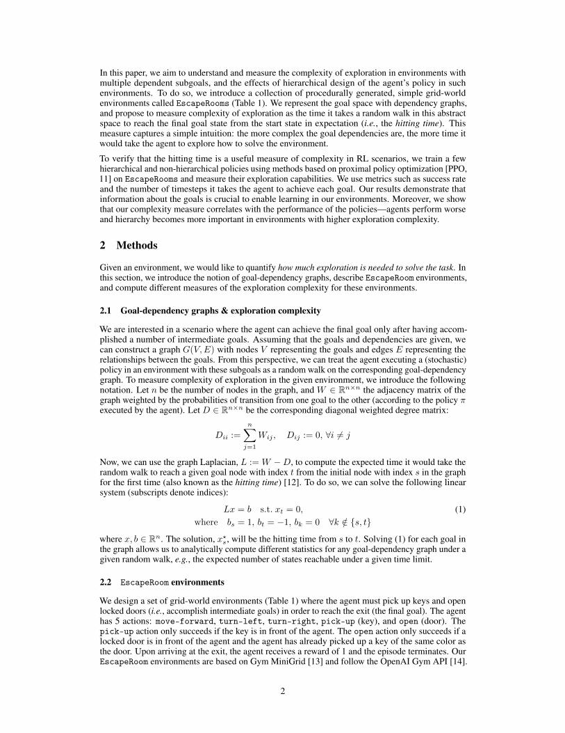
In this paper, we aim to understand and measure the complexity of exploration in environments withmultiple dependent subgoals, and the effects of hierarchical design of the agent’s policy in suchenvironments. To do so, we introduce a collection of procedurally generated, simple grid-worldenvironments called EscapeRooms (Table 1). We represent the goal space with dependency graphs,and propose to measure complexity of exploration as the time it takes a random walk in this abstractspace to reach the final goal state from the start state in expectation (i.e., the hitting time). Thismeasure captures a simple intuition: the more complex the goal dependencies are, the more time itwould take the agent to explore how to solve the environment.

To verify that the hitting time is a useful measure of complexity in RL scenarios, we train a fewhierarchical and non-hierarchical policies using methods based on proximal policy optimization [PPO,11] on EscapeRooms and measure their exploration capabilities. We use metrics such as success rateand the number of timesteps it takes the agent to achieve each goal. Our results demonstrate thatinformation about the goals is crucial to enable learning in our environments. Moreover, we showthat our complexity measure correlates with the performance of the policies—agents perform worseand hierarchy becomes more important in environments with higher exploration complexity.

2 Methods

Given an environment, we would like to quantify how much exploration is needed to solve the task. Inthis section, we introduce the notion of goal-dependency graphs, describe EscapeRoom environments,and compute different measures of the exploration complexity for these environments.

2.1 Goal-dependency graphs & exploration complexity

We are interested in a scenario where the agent can achieve the final goal only after having accom-plished a number of intermediate goals. Assuming that the goals and dependencies are given, wecan construct a graph G(V,E) with nodes V representing the goals and edges E representing therelationships between the goals. From this perspective, we can treat the agent executing a (stochastic)policy in an environment with these subgoals as a random walk on the corresponding goal-dependencygraph. To measure complexity of exploration in the given environment, we introduce the followingnotation. Let n be the number of nodes in the graph, and W ∈ Rn×n the adjacency matrix of thegraph weighted by the probabilities of transition from one goal to the other (according to the policy πexecuted by the agent). Let D ∈ Rn×n be the corresponding diagonal weighted degree matrix:

Dii :=

n∑j=1

Wij , Dij := 0, ∀i 6= j

Now, we can use the graph Laplacian, L :=W −D, to compute the expected time it would take therandom walk to reach a given goal node with index t from the initial node with index s in the graphfor the first time (also known as the hitting time) [12]. To do so, we can solve the following linearsystem (subscripts denote indices):

Lx = b s.t. xt = 0, (1)where bs = 1, bt = −1, bk = 0 ∀k /∈ {s, t}

where x, b ∈ Rn. The solution, x?s , will be the hitting time from s to t. Solving (1) for each goal inthe graph allows us to analytically compute different statistics for any goal-dependency graph under agiven random walk, e.g., the expected number of states reachable under a given time limit.

2.2 EscapeRoom environments

We design a set of grid-world environments (Table 1) where the agent must pick up keys and openlocked doors (i.e., accomplish intermediate goals) in order to reach the exit (the final goal). The agenthas 5 actions: move-forward, turn-left, turn-right, pick-up (key), and open (door). Thepick-up action only succeeds if the key is in front of the agent. The open action only succeeds if alocked door is in front of the agent and the agent has already picked up a key of the same color asthe door. Upon arriving at the exit, the agent receives a reward of 1 and the episode terminates. OurEscapeRoom environments are based on Gym MiniGrid [13] and follow the OpenAI Gym API [14].

2

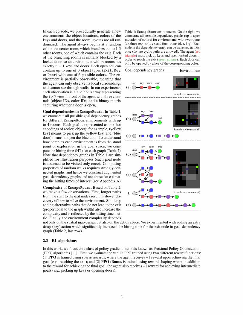
Table 1: EscapeRoom environments. On the right, weenumerate all possible dependency graphs (up to a per-mutation of colors) for environments with two rooms(a), three rooms (b, c), and four rooms (d, e, f ,g). Eachnode in the dependency graph can be traversed at mostonce (i.e., no cyclic paths are allowed). The agent (redtriangle) must pick up keys and open locked doors inorder to reach the exit (green square). Each door canonly be opened by a key of the corresponding color.

Goal dependency graphs Environment

(a)start key door exit

Sample environment (a)

(b)start

key door

exit

(c)

Sample environment (b)

(g)

(f)

(d)start

key door exit

(e)

Sample environment (f)

In each episode, we procedurally generate a newenvironment; the object locations, colors of thekeys and doors, and the room layouts are all ran-domized. The agent always begins at a randomcell in the center room, which branches out to 1-3other rooms, one of which contains the exit. Eachof the branching rooms is initially blocked by alocked door, so an environment with n rooms hasexactly n− 1 keys and doors. Each open cell cancontain up to one of 3 object types (Exit, Key,or Door) with one of 6 possible colors. The en-vironment is partially observable, meaning thatthe agent can only observe its local surroundingsand cannot see through walls. In our experiments,each observation is a 7× 7× 3 array representingthe 7×7 view in front of the agent with three chan-nels (object IDs, color IDs, and a binary matrixcapturing whether a door is open).

Goal dependencies in EscapeRooms. In Table 1,we enumerate all possible goal dependency graphsfor different EscapeRoom environments with upto 4 rooms. Each goal is represented as one-hotencodings of (color, object); for example, (yellowkey) means to pick up the yellow key, and (bluedoor) means to open the blue door. To understandhow complex each environment is from the standpoint of exploration in the goal space, we com-pute the hitting time (HT) for each graph (Table 2).Note that dependency graphs in Table 1 are sim-plified for illustration purposes (each goal nodeis assumed to be visited only once). Computingproperties of random walks requires strongly con-nected graphs, and hence we construct augmentedgoal-dependency graphs and use those for estimat-ing the hitting times of interest (see Appendix A).

Complexity of EscapeRooms. Based on Table 2,we make a few observations. First, longer pathsfrom the start to the exit nodes result in slower dis-covery of how to solve the environment. Similarly,adding alternative paths that do not lead to the exit(proportional to the graph width) also increase thecomplexity and is reflected by the hitting time met-ric. Finally, the environment complexity dependsnot only on the spatial map design but also on the action space. We experimented with adding an extradrop (key) action which significantly increased the hitting time for the exit node in goal-dependencygraph (Table 2, last row).

2.3 RL algorithms

In this work, we focus on a class of policy gradient methods known as Proximal Policy Optimization(PPO) algorithms [11]. First, we evaluate the vanilla PPO trained using two different reward functions:(1) PPO is trained using sparse rewards, where the agent receives +1 reward upon achieving the finalgoal (e.g., reaching the exit); and (2) PPO+Bonus is trained using reward shaping where in additionto the reward for achieving the final goal, the agent also receives +1 reward for achieving intermediategoals (e.g., picking up keys or opening doors).

3

Algorithm 1 Hierarchical PPO

1: Input: Meta-controller policy πM ,Controller policy πC

2: for i = 1 to num_episodes do3: subgoal g ← πM (s)4: while s is not terminal do5: F ← 06: s0 ← s7: while not (g is reached) do8: a← πC({s, g})9: state s′, reward f ← Env(a)

10: intrinsic reward r ← Critic(s′, g)11: PPO_update(πC , s, a, s′, r)12: F ← F + f13: s← s′

14: end while15: PPO_update(πM , s0, g, s′, F )16: subgoal g ← πM (s)17: end while18: end for

Next, we introduce a variant of PPO called HiPPO(Hierarchical PPO) which borrows the hierarchi-cal framework from [10], but replaces the hier-archical value functions in the h-DQN with hi-erarchical PPO policies. In more detail, HiPPOuses a meta-controller policy to choose interme-diate goals for the lower-level controller policy toachieve2. The controller receives one-hot encodedgoals as part of its observation and intrinsic re-wards for achieving intermediate goals chosen bythe meta-controller. The meta-controller receivessparse extrinsic rewards from the environment forachieving the final goal and is prompted to sub-mit a new action (i.e., a new goal) each time thelower-level controller accomplishes the previousgoal. The pseudocode for HiPPO is given in Al-gorithm 1. In our experiments, we used a fixedmeta-controller that chooses a sequence of goalsalong a random depth-first search path on the goaldependency graph, rather than a trainable meta-controller policy.

Lastly, PPO+Sketch is a variation of policy sketches [15] where the agent is provided with a sequenceof goals that leads to achieving the final goal. PPO+Sketch is identical to PPO except that in eachtimestep, the current observation is concatenated with the current intermediate goal3, i.e., the actionsproduced by the policy are always conditional on the current goal. Similar to PPO, and unlike HiPPOand PPO+Bonus, PPO+Sketch does not use intrinsic rewards for achieving intermediate goals.

3 Experiments

We evaluate PPO, PPO+Bonus, PPO+Sketch, and HiPPO on EscapeRoom environments (a)-(g). Welimit the episode length to 1000 time steps. For each method and environment, we use the LSTMpolicy with hidden dimension 64, and train for 10M total time steps on 128 vectorized environmentsusing the Adam optimizer, learning rate 2.5e-4, discount factor γ = 0.9, and TD λ = 0.95. Weevaluated each method and environment over 5 trials with different random seeds.

In Figure 1, we see that HiPPO consistently achieves the smallest average episode length and highestsuccess rate on all environments, thus demonstrating the benefit of using hierarchical policies thatoperate at different temporal scales. Surprisingly, PPO with sparse rewards performs better thanPPO+Bonus, showing that the bonus rewards for achieving intermediate goals does not help a non-hierarchical policy. We also find that PPO+Sketch performs worse than PPO indicating that merelyconditioning on subgoals might be suboptimal and destructively interferes with optimization.

Table 2: Depth, width, and hitting time (HT) statisticscomputed for EscapeRoom environments (a)-(g).

(a) (b) (c) (d) (e) (f) (g)

exit depth 2 2 4 2 2 4 6graph width 1 2 1 2 3 2 1HT (w/o drop-key) 8.4 12.1 15.1 13.1 13.9 29.2 27.5HT (w/ drop-key) 16.5 25.2 39.5 27.5 26.7 86.1 82.5

Environments (f) and (g) are more challengingfor RL agents due to greater exit depth of theirgoal dependency graphs, i.e., the agent mustachieve a longer sequence of intermediate goalsbefore it can reach the exit. Similarly, the widthof the dependency graph introduces complex-ity (due to paths that don’t lead anywhere), butnot as much as the depth. We find that the an-alytically estimated hitting times given in Table 2 are in agreement with the observed empiricalperformance of the RL algorithms. We also note that despite the complexity of the environments,HiPPO is still able to make some progress on (f) and (g), while the other flat PPO baselines (with orwithout reward shaping and/or policy sketches) fail to solve them (Figure 1).

2The action space of the meta-controller is the space of goals. The controller uses available primitive actions.3Feeding goals as observations into the policy network is slightly different from the original design of

Andreas et al. [15]. We plan to investigate the original policy sketch architecture in future work.

4

Table 3: Left: Average success rate (%) to reach the final goal over the last 10 training episodes. Right: Averageepisode length (% of the max length, smaller is more efficient) over the last 10 training episodes. “–” indicatesthat the method failed to reach the final goal within 1000 steps.

Average Success Rate Average Episode Length(a) (b) (c) (d) (e) (f) (g) (a) (b) (c) (d) (e) (f) (g)

PPO 56.1 28.2 0.2 22.7 19.1 0.0 0.0 78.5 88.0 – 90.7 91.4 – –PPO+Bonus 9.0 6.0 0.0 11.0 4.5 0.5 0.0 97.8 96.7 99.9 97.3 98.0 99.9 –PPO+Sketch 23.2 14.5 0.4 12.6 10.7 0.1 0.0 91.9 94.4 99.9 95.0 95.7 – –HiPPO 74.9 57.0 60.8 48.0 29.9 11.2 19.0 48.2 67.4 69.1 71.0 85.3 96.4 93.8

400

500

600

700

800

900

1000

episo

de le

ngth

(a) (b) (c) (d) (e) (f) (g)

2 4 6# timesteps 1e6

0.0

0.2

0.4

0.6

0.8

1.0

succ

ess r

ate

2 4 6# timesteps 1e6

2 4 6# timesteps 1e6

2 4 6# timesteps 1e6

2 4 6# timesteps 1e6

2 4 6# timesteps 1e6

2 4 6# timesteps 1e6

PPO PPO+Bonus HiPPO PPO+Sketch

Figure 1: Average episode length and success rate on EscapeRoom environments with goal dependency graphs(a)-(g) from Table 1. In all environments, HiPPO achieves the best performance (smallest episode length andhighest success rate). In the most complex environments (f) and (g), HiPPO still makes some learning progress.

100 200 300 400 500# episodes

100

200

300

400

500

600

700

800

900

1000

# st

eps t

ill go

al

Goal #1: Get first key

100 200 300 400 500# episodes

Goal #2: Open first door

100 200 300 400 500# episodes

Goal #3: Get second key

100 200 300 400 500# episodes

Goal #4: Open second door

100 200 300 400 500# episodes

Goal #5: Go to exit

PPO PPO+Bonus HiPPO PPO+Sketch

Figure 2: Average number of timesteps to reach each intermediate goal on EscapeRoom (c). HiPPO is thequickest method to achieve each goal.

10 15 20 25 30

hitting time10

20

30

40

50

60

70

succ

ess r

ate

(%)

(a)

(b)(c)

(d)

(e)

(f)(g)

10 15 20 25 30

hitting time

50

60

70

80

90

100

episo

de le

ngth

(%)

(a)

(b) (c)(d)

(e)

(f)(g)

Figure 3: Correlation between the hitting time (Table 2)vs. the average success rate and average episode length(Table 3) of HiPPO for EscapeRoom environments (a)-(g) from Table 1. This verifies that the hitting time is auseful measure of complexity for RL environments.

In Figure 3, we illustrate the correlation betweenthe hitting time on goal dependency graphs (Ta-ble 2) and the empirical performance of HiPPO(Table 3) for different EscapeRoom environ-ments, which demonstrates that analytically es-timated hitting time is an informative metric formeasuring the complexity of an environment.

4 Discussion

We designed a simple grid-world EscapeRoomenvironment where it is easy to measure theexploration complexity by analyzing the corre-sponding goal dependency graphs. We showedthat hitting times in goal dependency graphs are consistent with the empirical performance of PPO-based methods, and is therefore a useful metric to measure the complexity of the environment. Finally,we showed the performance improvement of HiPPO over other flat PPO baselines, demonstrating thebenefit of using hierarchical policies that operate at different temporal scales.

5

References[1] Sergey Levine, Chelsea Finn, Trevor Darrell, and Pieter Abbeel. End-to-end training of deep

visuomotor policies. The Journal of Machine Learning Research, 17(1):1334–1373, 2016.

[2] Volodymyr Mnih, Koray Kavukcuoglu, David Silver, Andrei A Rusu, Joel Veness, Marc GBellemare, Alex Graves, Martin Riedmiller, Andreas K Fidjeland, Georg Ostrovski, et al.Human-level control through deep reinforcement learning. Nature, 518(7540):529–533, 2015.

[3] David Silver, Julian Schrittwieser, Karen Simonyan, Ioannis Antonoglou, Aja Huang, ArthurGuez, Thomas Hubert, Lucas Baker, Matthew Lai, Adrian Bolton, et al. Mastering the game ofgo without human knowledge. Nature, 550(7676):354, 2017.

[4] Christoph Dann, Katja Hofmann, and Sebastian Nowozin. Memory lens: How much memorydoes an agent use? arXiv preprint arXiv:1611.06928, 2016.

[5] Marc Bellemare, Sriram Srinivasan, Georg Ostrovski, Tom Schaul, David Saxton, and RemiMunos. Unifying count-based exploration and intrinsic motivation. In Advances in NeuralInformation Processing Systems, pages 1471–1479, 2016.

[6] Meire Fortunato, Mohammad Gheshlaghi Azar, Bilal Piot, Jacob Menick, Ian Osband, AlexGraves, Vlad Mnih, Remi Munos, Demis Hassabis, Olivier Pietquin, et al. Noisy networks forexploration. arXiv preprint arXiv:1706.10295, 2017.

[7] Matthias Plappert, Rein Houthooft, Prafulla Dhariwal, Szymon Sidor, Richard Y Chen, Xi Chen,Tamim Asfour, Pieter Abbeel, and Marcin Andrychowicz. Parameter space noise for exploration.arXiv preprint arXiv:1706.01905, 2017.

[8] Richard S Sutton, Doina Precup, and Satinder Singh. Between mdps and semi-mdps: Aframework for temporal abstraction in reinforcement learning. Artificial intelligence, 112(1-2):181–211, 1999.

[9] Pierre-Luc Bacon, Jean Harb, and Doina Precup. The option-critic architecture. In AAAI, pages1726–1734, 2017.

[10] Tejas D Kulkarni, Karthik Narasimhan, Ardavan Saeedi, and Josh Tenenbaum. Hierarchicaldeep reinforcement learning: Integrating temporal abstraction and intrinsic motivation. InAdvances in neural information processing systems, pages 3675–3683, 2016.

[11] John Schulman, Filip Wolski, Prafulla Dhariwal, Alec Radford, and Oleg Klimov. Proximalpolicy optimization algorithms. arXiv preprint arXiv:1707.06347, 2017.

[12] László Lovász. Random walks on graphs. Combinatorics, Paul erdos is eighty, 2(1-46):4, 1993.

[13] Maxime Chevalier-Boisvert and Lucas Willems. Minimalistic Gridworld Environment forOpenAI Gym. https://github.com/maximecb/gym-minigrid, 2018.

[14] Greg Brockman, Vicki Cheung, Ludwig Pettersson, Jonas Schneider, John Schulman, Jie Tang,and Wojciech Zaremba. Openai gym. arXiv preprint arXiv:1606.01540, 2016.

[15] Jacob Andreas, Dan Klein, and Sergey Levine. Modular multitask reinforcement learning withpolicy sketches. arXiv preprint arXiv:1611.01796, 2016.

6

A Details on computing hitting times

As we mentioned in Section 2.3, to compute the hitting time of random walk we need an augmentedgoal-dependency graph (which can be generated procedurally from the graphs given in the main text).An example augmented graph for EscapeRoom (c) from Table 1 is presented below.

start

All doors closed

key 1

room 1

start

First door open

key 2

room 2room 1

start

Both doors open

exit

Found exit

The main difference from the goal dependency graph given in Table 1 is that when the agent picks upa key and opens the corresponding door, it transitions into a subgraph that corresponds to the newlayout of the rooms accessible to the agent. Self-loops and transitions between the rooms representthe moving behavior.

We set the following parameters for the random walk. With 80% chance, no transition happens. With19% chance, the walk transitions from the current node along one of the outgoing edges. Finally, toensure strong connectivity of the graph, we add 1% chance of the agent moving back to the root startnode from any other node in the graph4. This corresponds to the situation where the agent is not ableto reach the exit within the time limit and must start a new episode.

4A similar approach is taken by the PageRank algorithm.

7