On the Complexity of Computing Gröbner Basesfor Quasi-Homogeneous Systems

Jean-Charles Faugère*

Jean-Charles.Faugere@inria.frMohab Safey El Din*‡

Mohab.Safey@lip6.frThibaut Verron†*

Thibaut.Verron@ens.fr*INRIA, Paris-Rocquencourt Center, PolSys Project ‡Institut Universitaire de France

UPMC, Univ. Paris 06, LIP6CNRS, UMR 7606, LIP6 †École Normale Supérieure,

Case 169, 4, Place Jussieu, F-75252 Paris 45, rue d’Ulm, F-75230, Paris

ABSTRACTLet K be a field and ( f1, . . . , fn) ⊂ K[X1, . . . ,Xn] be a sequence ofquasi-homogeneous polynomials of respective weighted degrees(d1, . . . ,dn) w.r.t a system of weights (w1, . . . ,wn). Such systemsare likely to arise from a lot of applications, including physics orcryptography.

We design strategies for computing Gröbner bases for quasi-homogeneous systems by adapting existing algorithms for homo-geneous systems to the quasi-homogeneous case. Overall, undergenericity assumptions, we show that for a generic zero-dimensionalquasi-homogeneous system, the complexity of the full strategy ispolynomial in the weighted Bézout bound ∏

ni=1 di/∏

ni=1 wi.

We provide some experimental results based on generic systemsas well as systems arising from a cryptography problem. They showthat taking advantage of the quasi-homogeneous structure of thesystems allow us to solve systems that were out of reach otherwise.

Categories and Subject DescriptorsI.1.2 [Symbolic and Algebraic Manipulation]: Algorithms; F.2.2[Analysis of Algorithms and Problem Complexity]: Nonnumeri-cal Algorithms and Problems

KeywordsGröbner bases; Polynomial system solving; Quasi-homogeneouspolynomials

1. INTRODUCTIONPolynomial system solving is a very important problem in com-

puter algebra, with a wide range of applications in theory (algo-rithmic geometry) or in real life (cryptography). For that purpose,Gröbner bases of polynomial ideals are a valuable tool, and practica-ble computation of the Gröbner bases of any given ideal is a majorchallenge of modern computer algebra. Since their introductionin 1965, many algorithms have been designed to compute Gröbnerbases ([6, 9, 10, 11]), improving the efficiency of the computations.

Permission to make digital or hard copies of all or part of this work forpersonal or classroom use is granted without fee provided that copies arenot made or distributed for profit or commercial advantage and that copiesbear this notice and the full citation on the first page. To copy otherwise, torepublish, to post on servers or to redistribute to lists, requires prior specificpermission and/or a fee.ISSAC’13, June 26–29, 2013, Boston, Massachusetts, USA.Copyright 2013 ACM 978-1-4503-2059-7/13/06 ...$15.00.

Systems arising from “real life” problems often have some struc-ture. It has been observed that most of these structures can makethe Gröbner basis easier to compute. For example, it is known thathomogeneous systems, or systems with an important maximal homo-geneous component, are better solved by using a degree-compatibleorder, and then applying a change of ordering. In this paper, westudy a structure slightly more general than homogeneity, calledquasi-homogeneity. More precisely, we will say that a polyno-mial P(X1, . . . ,Xn) is quasi-homogeneous for the system of weightsW = (w1, . . . ,wn), if the polynomial

Q(Y1, . . . ,Yn) := P(Y w11 , . . . ,Y wn

n )

is homogeneous. Systems with such a structure are likely to arisefor example from physics, where all measures are associated with adimension which, to some extent, can be seen as a weight.

Let F = ( f1, . . . , fm) be a system of polynomials, in a polynomialalgebra graded w.r.t the system of weights W = (w1, . . . ,wn). In thefollowing, we will assume that F is quasi-homogeneous and generic,or more generally that its quasi-homogeneous components of maxi-mal weighted degree are generic. It is possible to compute directlya Gröbner basis of the ideal generated by F . This strategy consistsof running the classical algorithms F5 ([10]) and FGLM ([11]) onF , while ignoring the quasi-homogeneous structure. However, tothe best of our knowledge, there is no general way of evaluating thecomplexity of that strategy.

Another approach is to compute the homogenized system definedby F := ( fi(X

w11 , . . . ,Xwn

n )), and then compute a Gröbner basis ofthat system, using the usual strategies for the homogeneous struc-ture. Experimentally, the first step of the computation is much fasterthan with the naive strategy. However, the number of solutions is in-creased by a factor of ∏

ni=1 wi, slowing down the change of ordering,

which thus becomes the main bottleneck of the computation.Furthermore, to the best of our knowledge, the best complexity

bounds for this computation are those we obtain for a homoge-neous system of the same degree. However, experimentally, thefirst step of the computation proves faster for a homogenized quasi-homogeneous system with weighted degree (d1, . . . ,dn) than for ahomogeneous system of total degree (d1, . . . ,dn).Main results. We provide a complexity study of the above strat-egy, allowing us to quantify this speed-up, as well as to proposea workaround for the change of ordering. Overall, we prove thatthe known bounds for this strategy can be divided by ∏

ni=1 wi for

a generic zero-dimensional W -homogeneous system with weightsW = (w1, . . . ,wn).

More precisely, we assume the system ( f1, . . . , fm) to satisfy thetwo following generic assumptions:

H1. The sequence f1, . . . , fm is regular;

189

H2. The sequence f1, . . . , fi is in Noether position w.r.t. X1, . . . ,Xi,for any 1≤ i≤ m.

Under hypothesis H1, we adapt the classical results of the homo-geneous case, using similar arguments based on Hilbert series, toestimate the degree of the ideal and the degree of regularity of thesystem:

deg(I) =n

∏i=1

di

wi; dreg(F)≤

n

∑i=1

(di−wi

)+max{wi}.

We study the complexity of the F5 algorithm through its matrixvariant matrix-F5. This is a usual approach, carried on for examplein [14]. With minor changes, the matrix-F5 algorithm for homoge-neous systems can be adapted to quasi-homogeneous systems. Acombinatorial result found in [1] shows that the number of columnsof the matrices appearing in that variant of matrix-F5 is approxi-mately smaller by a factor of ∏

ni=1 wi, when compared to the regular

matrix-F5 algorithm. Overall, we can obtain complexity boundswhich are smaller by a factor of Pω than the bounds we wouldobtain for a generic homogeneous system with same degrees, whereP = ∏

ni=1 wi and ω is the exponent of the complexity of matrix mul-

tiplication. In the end, we show that for systems satisfying H1, ourstrategy, running F5 on the homogenized system, dehomogenizingthe result, and then running FGLM, performs in time polynomial in∏

ni=1 di/∏

ni=1 wi, that is polynomial in the number of solutions.

Further assuming hypothesis H2, we also carry on the precisecomplexity analyses done in [2] for homogeneous systems, andadapt them to the quasi-homogeneous case to deduce a precisecomplexity bound for our quasi-homogeneous variant of Matrix-F5. These new complexity bounds are also smaller by a factor ofPω than similar bounds for a generic homogeneous system. Eventhough these bounds still do not match exactly the experimentalcomplexity, they tend to confirm that overall, we are able to computea LEX Gröbner basis for a generic quasi-homogeneous system intime reduced by a factor of Pω , when compared with a generichomogeneous system with same degrees.

We have run benchmarks with the FGb library ([16]) and theMagma computer algebra software ([5]), on both generic systemsand real-life systems arising in cryptography. Experimentally, inboth cases, our strategy seems always faster than ignoring the quasi-homogeneous structure, and the speed-up increases with the consid-ered weights.

Experiments have also shown that the order of the variables canhave an impact on the performances of both strategies. Predictingthis behavior seems to require more sophisticated tools and may bematerial for future research.Prior works. Making use of the structure of polynomial systemsto develop faster algorithms has been a general trend over the pastfew years: see for example [12], [7] or [15]. Polynomial algebrasgraded with respect to a system of weights have been studied byresearchers in commutative algebra. Most notably, the Hilbert seriesof ideals defined by regular sequences, which we use several timesin this paper, is well known, and could be found for example in [21].The paper [20] defines many structures of polynomial algebras, in-cluding weighted gradings, in preparation for future algorithmicdevelopments. Combinatorial objects arising when we try to es-timate the number of monomials of a given W -degree are calledSylvester denumerants, and studied for example in [1].

When it comes to Gröbner bases, weighted gradings and relatedorderings have been described in early works such as [4]. However,as far as we know, the impact of a quasi-homogeneous structureon the complexity of Gröbner bases computations had never beenstudied.

Among the various computer algebra software able to computeGröbner bases, it seems that only Magma has algorithms dedicated

to quasi-homogeneous systems. Given a quasi-homogeneous system,it will detect the appropriate system of weights, and use the W -GREVLEX ordering to compute an intermediate basis before thechange of ordering. However, this strategy is only available forquasi-homogeneous systems, while it can be useful in many othercases, for example systems of polynomials defined as the sum of aquasi-homogeneous component and a scalar.

Other computer algebra software (e.g. Singular) allow the userto compute F and to run the Gröbner basis algorithm on it. Sinceall these algorithms (most often Buchberger, F4 or F5) use S-pairs,they will show a similar speed-up. However, the user must noticethat the computations may benefit from using a quasi-homogeneousstructure of the system, and provide the system of weights.

We do not provide a way to know what is the “appropriate” systemof weights for a given system, or even to detect systems which wouldbenefit from taking into account the quasi-homogeneous structure.However, some systems obviously belong to that category (e.g quasi-homogeneous plus scalar), and the system of weights will then beeasy to compute.Structure of the paper. In section 2 we define more preciselyquasi-homogeneous systems, and we compute their degree anddegree of regularity assuming the above hypotheses. We also takethis opportunity to show briefly that these hypotheses are generic.In section 3 we prove that the strategy consisting of modifyingthe system is correct, we explain how we can adapt matrix-F5 andFGLM to quasi-homogeneous systems, and then we evaluate thecomplexity of these algorithms. In section 4, we briefly explainhow these results for quasi-homogeneous systems still help in casethe system was obtained from a quasi-homogeneous system byspecializing one of the variables to 1. We also give an example ofsuch a structure, as well as the associated algorithm. Finally, insection 5, we give some experimental results.

2. QUASI-HOMOGENEOUS SYSTEMS2.1 Weighted degrees and polynomialsLet K be a field. We consider the algebra A :=K[X1, . . . ,Xn] =K[X].Even though one usually uses the total degree to grade the algebraA, there are other ways to define such a grading, as seen in [4], forexample.

Definition 1. Let W = (w1, . . . ,wn) be a vector of positive inte-gers. Let α = (α1, . . . ,αn) be a tuple of nonnegative integers. Letthe integer degW (Xα ) = ∑

ni=1 wiαi be the W-degree, or weighted

degree of the monomial Xα = Xα11 · · ·X

αnn . Call the vector W a sys-

tem of weights. We denote by 1 the system of weights defined by(1, . . . ,1), associated with the usual grading on A.

One can prove that any grading on K[X] comes from such asystem of weights ([4, sec. 10.2]). We denote by (K[X],W ) theW -graded structure on A, and in that case, to clear ambiguities, weuse the adjective W-homogeneous for elements or ideals, or quasi-homogeneous or weighted homogeneous if W is clear in the context.The word homogeneous will be reserved for 1-homogeneous items.

PROPOSITION 1. Let (K[X1, . . . ,Xn],W ) be a graded polyno-mial algebra. Then the application

homW : (K[X1, . . . ,Xn],W ) → (K[t1, . . . , tn],1)f 7→ f (tw1

1 , . . . , twnn )

is an injective graded morphism, and in particular the image of aquasi-homogeneous polynomial is a homogeneous polynomial.

PROOF. It is an easy consequence of the definition of the gradingw.r.t a system of weights.

The above morphism also provides a quasi-homogeneous variantof the GREVLEX ordering (as found for example in [4]), which we

190

call the W-GREVLEX ordering:u <W -grevlex v ⇐⇒ homW (v)<grevlex homW (v)

Given a W -homogeneous system F , one can build the homogeneoussystem homW (F), and then apply classical algorithms ([10, 11])to that system to compute a GREVLEX (resp. LEX) Gröbner basisof the ideal generated by homW (F). We will prove in section 3(prop. 7) that this basis is contained in the image of homW , and thatits pullback is a W -GREVLEX (resp. LEX) Gröbner basis of theideal generated by F .

Let us end this paragraph with some notations and definitions.The degree of regularity of the system F is the highest degree dreg(F)reached in a run of F5 to compute a GREVLEX Gröbner basis ofhomW (F). The index of regularity of an ideal I is the degree ireg ofthe Hilbert series HSA/I , defined as the difference of the degree ofits numerator and the degree of its denominator.

Recall that given a homogeneous ideal I, we define its degree D asthe degree of the projective variety V (I), as introduced for examplein [18]. This definition still holds for the quasi-homogeneous case.In case the projective variety is empty, that is if the affine variety isequal to {0}, we extend that definition by letting D be the multiplic-ity of the 0 point, that is the dimension of the K-vector space A/I.Finally, from now on we will only consider affine varieties, evenwhen the ideal is quasi-homogeneous. In particular, the dimensionof V (0) is n, and that a zero-dimensional variety will be defined byat least n polynomials.

2.2 Degree and degree of regularityZero-dimensional regular sequences. As in the homoge-neous case, regular sequences are an important case to study, be-cause it is a generic property which allows us to compute severalkey parameters and good complexity bounds. We first characterizethe degree and bound the degree of regularity of a zero-dimensionalideal defined by a regular sequence.

THEOREM 2. Let W = (w1, . . . ,wn) be a system of weights, andF = ( f1, . . . , fm) a regular sequence of W-homogeneous polyno-mials, of respective W-degrees d1, . . . ,dm. Further assume thatthe set of solutions is zero-dimensional, that is m = n. We denoteby I the quasi-homogeneous ideal generated by F. Then we havedeg(I) = ∏

ni=1

diwi

and dreg(F)≤ ∑ni=1(di−wi

)+max{wi}.

PROOF. We will determine the degree and degree of regularityof the system from the Hilbert series (or Poincaré series) of thealgebra A/I. A classical result which can be found for examplein [21, cor. 3.3] states that, for regular sequences, this series is

HSA/I(t) =(1− td1) · · ·(1− tdm)

(1− tw1) · · ·(1− twn). (1)

We assumed n = m, so the Hilbert series can be rewritten as

HSA/I(t) =(1+ · · ·+ td1−1) · · ·(1+ · · ·+ tdn−1)

(1+ · · ·+ tw1−1) . . .(1+ · · ·+ twn−1).

In the 0-dimensional case, recall that the Hilbert series is actually apolynomial, and has degree ireg = ∑

ni=1(di−wi). This means that

all monomials of W -degree greater than ireg are in the ideal, and assuch, that the leading terms of the W -GREVLEX Gröbner basis of Fneed to divide all the monomials of W -degree greater than ireg.Thisproves that all the polynomials in the Gröbner basis computed by F5have W -degree at most ireg +max{wi}. And since the F5 criterion([10]) ensures that there is no reduction to zero in a run of F5 ona regular sequence, the algorithm indeed stops in degree at mostireg +max{wi}.

Furthermore, the degree of the ideal I is equal to the dimension ofthe vector space A/I, that is the value of the Hilbert series at t = 1,that is ∏

ni=1

diwi

.

Note that except for this inequality, not much is known about thedegree of regularity of a quasi-homogeneous system. In particular,the above bound is nothing more than a bound, even in the genericcase. Let us introduce some examples of the three cases one canobserve with a quasi-homogeneous generic system:

1. W = (3,2,1), generic system of W -degree D = (6,6,6): thendreg = ireg +1 = 13;

2. W = (1,2,3), generic system of W -degree D = (6,6,6): thendreg = 15 > ireg +1 = 13;

3. W = (2,3), generic system of W -degree D = (6,6): thendreg = 6 < ireg = 7.

Only the case 1 is observed with generic homogeneous systems.Furthermore, examples 1 and 2 show that the degree of regularitydepends upon the order of the variables (chosen in the description ofthe system of weights). As the Hilbert series of a generic sequencedoesn’t depend on that order, it shows that we probably need to find abetter tool in order to evaluate more precisely the degree of regularityin the quasi-homogeneous case. However, the above bound alreadyleads to good improvements on the complexity bounds, as we willsee in the following sections. Also note that these computationsonly hold when the system is 0-dimensional, we will discuss thatrestriction in section 2.3.

Genericity. We now prove that zero-dimensional W -homoge-neous sequences of given W -degree are generically regular, undersome assumptions on the W -degree. Let us start with the first partof this statement:

LEMMA 3. Let n be a positive integer, and consider the algebraA := K[X1, . . . ,Xn], graded with respect to the system of weightsW = (w1, . . . ,wn). Regular sequences of length n form a Zariski-open subset of all sequences of quasi-homogeneous polynomials ofgiven W-degree in A.

PROOF. Let (d1, . . . ,dm) be a family of W -degrees, we considerthe set V (K[a][X]) of all systems of quasi-homogeneous polynomi-als of W -degree d1, . . . ,dm, where a is a set of variables representingthe coefficients of the polynomials. We denote by f1, . . . , fm thepolynomials of the generic system, and by I the ideal they generate,in K[a][X].

Since the Hilbert series (1) characterizes regular sequences ([21,cor. 3.2]), the sequence ( fi) is regular if and only if the idealI contains all monomials of W -degree between ireg(I) + 1 andireg(I)+max{wi}, where ireg(I) is given by ∑(di−wi). This ex-presses that a given set of linear equations has solutions, and so itcan be coded as some determinants being non-zero.

There are some systems of W -degree for which there is no regularsequence. The reason is that because of the weights, for somesystems of W -degrees, there exists no or very few monomials.For example, take n = 2, W = (1,2) and D = (1,1). All quasi-homogeneous polynomials of W -degree 1 are in KX , so there isno regular sequence of quasi-homogeneous polynomials with theseW -degrees.

However, if we only consider “reasonable” systems of W -degrees,that is systems of W -degrees for which there exists a regular se-quence, regular sequences form a Zariski-dense subset from theabove.

Remark 1. A sufficient condition for example is to take weighteddegrees such that d1 is divisible by w1, . . . , dn is divisible by wn.Thus we can define the sequence X

d1/w1

1 , . . . ,Xdn/wn

n , which is regular,and so for such systems of weight, the regularity condition is generic.

We only proved the genericity for quasi-homogeneous sequencesof length n, the more general case of a sequence of length m ≤ nwill be proved in section 2.3 (remark 2).

191

2.3 Noether positionTo compute the degree and degree of regularity of quasi-homoge-

neous systems of positive dimension, we will assume that the systemF = ( f1, . . . , fm) we consider is in Noether position (as seen in [8,ch. 13, sec. 1] or [3, def. 2]), i.e. the ideal I = 〈F〉 satisfies the twofollowing conditions:• for i≤m, the canonical image of Xi in K[X]/I is an algebraic

integer over K[Xm+1, . . . ,Xn];• K[Xm+1, . . . ,Xn]∩ I = 0.

LEMMA 4. Let F = f1, . . . , fm be a regular quasi-homogeneoussequence of polynomials in K[X1, . . . ,Xn]. The sequence F is inNoether position if and only if Fext := f1, . . . , fm,Xm+1, . . . ,Xn is aregular sequence.

PROOF. Let I be the ideal generated by the fi’s. The geometriccharacterization of Noether position (see e.g. [19]) shows that thecanonical projection onto the m first coordinates

π : V (I)→V (〈X1, . . . ,Xm〉)is a surjective morphism with finite fibers. This implies that thevariety V (〈Fext〉), that is π−1(0), is zero-dimensional, and so thesequence is regular.

Conversely, assume Fext is a regular sequence. Let i ≤ m, wewant to show that Xi is integral over the ring K[Xm+1, . . . ,Xn]. SinceFext defines a zero-dimensional ideal, there exists ni ∈ N suchthat Xni

i = LT( f ) with f ∈ 〈Fext〉 for the GREVLEX ordering withX1 > · · ·> Xn. By definition of the GREVLEX ordering, we can as-sume that f simply belongs to I. This shows that every Xi is integralover K[Xi+1, . . . ,Xn]/I. We get the requested result by inductionon i : first, this is clear if i = m. Now assume that we know thatK[Xi, . . . ,Xn]/I is an integral extension of K[Xm+1, . . . ,Xn]. Fromthe above, we also know that Xi−1 is integral over K[Xi, . . . ,Xn], andso, since the composition of integral homomorphisms is integral, weget the requested result.

Finally, we want to check the second part of the definition ofNoether position. Assume that there is a non-zero polynomialin K[Xm+1, . . . ,Xn]∩ I, since the ideal is quasi-homogeneous, wecan assume this polynomial to be quasi-homogeneous. Either thispolynomial is of degree 0, or it is a non-trivial syzygy betweenXm+1, . . . ,Xn. So in any case, it contradicts the regularity hypothe-sis.

As we did for regular sequences, we first show how we can eval-uate the degree and degree of regularity of a sequence in Noetherposition, and then we show that the Noether position property isgeneric under some assumptions on the W -degree of the polynomi-als.

THEOREM 5. Let W = (w1, . . . ,wn) be a system of weights, andf1, . . . , fm a regular sequence in Noether position, of quasi-homoge-neous polynomials of W-degrees (d1, . . . ,dm). The same way we didabove, we denote by I the ideal generated by the fi’s. Then we havedeg(I) = ∏

mi=1

diwi

and dreg(I)≤ ∑mi=1(di−wi

)+max{wi}.

PROOF. Let us denote by I′ the ideal generated by Fext. Thedegree of the ideal I′ is the same as that of I, because the varietyit defines is the intersection of V (I) with some non-zero-divisorhyperplanes. Furthermore, all critical pairs appearing in a runof F5 on F will also appear in a run of F5 on Fext, ensuring thatdreg(F)≤ dreg(Fext).

But since by Noether position, the family Fext defines a zero-dimensional variety, we can use the previous computations to deduceits degree of regularity and the degree of I′.

LEMMA 6. Let n be a positive integer, and consider the algebraA := K[X1, . . . ,Xn], graded with respect to the system of weightsW = (w1, . . . ,wn). Systems in Noether position form a Zariski-opensubset of all systems of quasi-homogeneous polynomials of givenW-degrees in A.

PROOF. Let F = ( f1, . . . , fm) be m generic quasi-homogeneouspolynomials, with coefficients in K[a]. We use the same characteri-zation of a zero-dimensional regular sequence as we did in the proofof Lemma 3. It allows us to express the regularity condition forthe sequence ( f1, . . . , fm,Xm+1, . . . ,Xn) as some determinants beingnon-zero, which by definition, shows that the condition of being inNoether position is an open condition.

Since a sequence in Noether position is in particular a regularsequence, we are confronted with the same problem as for the gener-icity of regular sequences, that is the possible emptiness of thecondition. However, it is still true that for “reasonable” systems ofW -degrees, i.e. systems of W -degrees for which there exists enoughmonomials, sequences in Noether position do exist, and thus forma Zariski-dense subset of all sequences. For example, since thesequence X

d1/w1

1 , . . . ,Xdm/wm

m is in Noether position, the sufficient con-dition given in Remark 1 is also sufficient to ensure that sequencesin Noether position are Zariski-dense.

Remark 2. Any sequence in Noether position is in particular aregular sequence, so Lemma 6 proves that, under the same assump-tion on the degree, regular sequences of length m ≤ n are genericamong quasi-homogeneous sequences of given W -degree.

3. COMPUTING GRÖBNER BASES3.1 Using the standard algorithms on the

ho-mogenized systemAs we said before, in order to apply the F5 algorithm to a quasi-

homogeneous system, we may run it through homW . This is shownby the following proposition.

PROPOSITION 7. Let F = ( f1, . . . , fm) be a family of polynomi-als in K[X1, . . . ,Xn], assumed to be quasi-homogeneous for a systemof weights W = (w1, . . . ,wn). Let <1 be a monomial order, G thereduced Gröbner basis of homW (F) for this order, and <2 thepullback of <1 through homW . Then

1. all elements of G are in the image of homW ;2. the family G′ := hom−1

W (G) is a reduced Gröbner basis of thesystem F for the order <2.

PROOF. The morphism homW preserves S-polynomials, in thesense that S-Pol(homW ( f ), homW (g)) = homW (S-Pol( f ,g)). Re-call that we can compute a reduced Gröbner basis by running theBuchberger algorithm, which involves only multiplications, addi-tions, tests of divisibility and computation of S-polynomials. Sinceall these operations are compatible with homW , if we run the Buch-berger algorithm on both F and homW (F) simultaneously, they willfollow exactly the same computations up to application of homW .The consequences on the final reduced Gröbner basis follow.

In practice, if we want to compute a LEX Gröbner basis of F ,we generate the system F = homW (F), we compute a GREVLEX

basis G1 of F with F5, and then we compute a LEX Gröbner basisG2 of F with FGLM. In the end, we get a LEX Gröbner basis of F ,which we turn into a LEX Gröbner basis of F via hom−1

W .

3.2 Direct algorithmsWe can now explain why algorithm FGLM becomes a bottleneck

with the above strategy. Indeed, we have seen that going throughhomW increases the Bézout bound of the system by a factor ∏

ni=1 wi,

and recall that the complexity of the FGLM step is polynomial inthat bound.

Here is a workaround. In the above process, we can apply hom−1W

to the basis G1 and thus obtain a W -GREVLEX basis G1 of F . We

192

can then run FGLM on that basis to obtain a LEX basis of F . Thus,we can avoid the problem of a greater degree of the ideal on thecomplexity of the FGLM step.

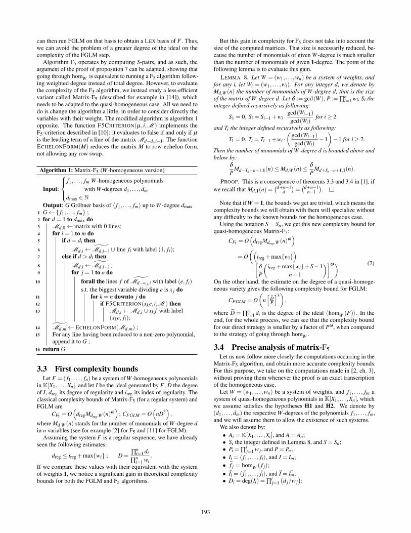
Algorithm F5 operates by computing S-pairs, and as such, theargument of the proof of proposition 7 can be adapted, showing thatgoing through homW is equivalent to running a F5 algorithm follow-ing weighted degree instead of total degree. However, to evaluatethe complexity of the F5 algorithm, we instead study a less-efficientvariant called Matrix-F5 (described for example in [14]), whichneeds to be adapted to the quasi-homogeneous case. All we need todo is change the algorithm a little, in order to consider directly thevariables with their weight. The modified algorithm is algorithm 1opposite. The function F5CRITERION(µ, i,M ) implements theF5-criterion described in [10]: it evaluates to false if and only if µ

is the leading term of a line of the matrix Md−di,i−1. The functionECHELONFORM(M) reduces the matrix M to row-echelon form,not allowing any row swap.

Algorithm 1: Matrix-F5 (W -homogeneous version)

Input:

f1, . . . , fm W -homogeneous polynomials

with W -degrees d1, . . . ,dm

dmax ∈ NOutput: G Gröbner basis of 〈 f1, . . . , fm〉 up to W -degree dmax

1 G←{ f1, . . . , fm} ;2 for d = 1 to dmax do3 Md,0← matrix with 0 lines;4 for i = 1 to m do5 if d = di then6 Md,i← Md,i−1∪ line fi with label (1, fi);7 else if d > di then8 Md,i← Md,i−1;9 for j = 1 to n do

10 forall the lines f of Md−w j ,i with label (e, fi)s.t. the biggest variable dividing e is x j do

11 for k = n downto j do12 if F5CRITERION(xke, i,M ) then13 Md,i←Md,i ∪ xk f with label

(xke, fi);

14 Md,m← ECHELONFORM(Md,m) ;15 For any line having been reduced to a non-zero polynomial,

append it to G ;16 return G

3.3 First complexity boundsLet F = ( f1, . . . , fn) be a system of W -homogeneous polynomials

in K[X1, . . . ,Xn], and let I be the ideal generated by F , D the degreeof I, dreg its degree of regularity and ireg its index of regularity. Theclassical complexity bounds of Matrix-F5 (for a regular system) andFGLM are

CF5 = O(

dregMdreg,W (n)ω)

; CFGLM = O(

nD3),

where Md,W (n) stands for the number of monomials of W -degree din n variables (see for example [2] for F5 and [11] for FGLM).

Assuming the system F is a regular sequence, we have alreadyseen the following estimates:

dreg ≤ ireg +max{wi} ; D =∏

ni=1 di

∏ni=1 wi

.

If we compare these values with their equivalent with the systemof weights 1, we notice a significant gain in theoretical complexitybounds for both the FGLM and F5 algorithms.

But this gain in complexity for F5 does not take into account thesize of the computed matrices. That size is necessarily reduced, be-cause the number of monomials of given W -degree is much smallerthan the number of monomials of given 1-degree. The point of thefollowing lemma is to evaluate this gain.

LEMMA 8. Let W = (w1, . . . ,wn) be a system of weights, andfor any i, let Wi = (w1, . . . ,wi). For any integer d, we denote byMd,W (n) the number of monomials of W-degree d, that is the sizeof the matrix of W-degree d. Let δ := gcd(W ), P := ∏

ni=1 wi, Si the

integer defined recursively as following:

S1 = 0, Si = Si−1 +wi ·gcd(Wi−1)

gcd(Wi)for i≥ 2

and Ti the integer defined recursively as following:

T1 = 0, Ti = Ti−1 +wi ·(

gcd(Wi−1)

gcd(Wi)−1)−1 for i≥ 2.

Then the number of monomials of W-degree d is bounded above andbelow by:

δ

PMd−Tn−n+1,1(n)≤Md,W (n)≤ δ

PMd+Sn−n+1,1(n).

PROOF. This is a consequence of theorems 3.3 and 3.4 in [1], ifwe recall that Md,1(n) =

(d+n−1d)=(d+n−1

n−1).

Note that if W = 1, the bounds we get are trivial, which means thecomplexity bounds we will obtain with them will specialize withoutany difficulty to the known bounds for the homogeneous case.

Using the notation S = Sn, we get this new complexity bound forquasi-homogeneous Matrix-F5:

CF5 = O(

dregMdreg,W (n)ω)

= O((

ireg +max{wi})

·[

δ

P

(ireg +max{wi}+S−1

n−1

)]ω).

(2)

On the other hand, the estimate on the degree of a quasi-homoge-neous variety gives the following complexity bound for FGLM:

CFGLM = O(

n[

DP

]3),

where D = ∏ni=1 di is the degree of the ideal 〈homW (F)〉. In the

end, for the whole process, we can see that the complexity boundfor our direct strategy is smaller by a factor of Pω , when comparedto the strategy of going through homW .

3.4 Precise analysis of matrix-F5Let us now follow more closely the computations occurring in the

Matrix-F5 algorithm, and obtain more accurate complexity bounds.For this purpose, we take on the computations made in [2, ch. 3],without proving them whenever the proof is an exact transcriptionof the homogeneous case.

Let W = (w1, . . . ,wn) be a system of weights, and f1, . . . , fm asystem of quasi-homogeneous polynomials in K[X1, . . . ,Xn], whichwe assume satisfies the hypotheses H1 and H2. We denote by(d1, . . . ,dm) the respective W -degrees of the polynomials f1, . . . , fm,and we will assume them to allow the existence of such systems.

We also denote by:• Ai =K[X1, . . . ,Xi], and A = An;• Si the integer defined in Lemma 8, and S = Sn;• Pi = ∏

ij=1 w j, and P = Pn;

• Ii = 〈 f1, . . . , fi〉, and I = Im;• f j = homW ( f j);• Ii = 〈 f1, . . . , fi〉, and I = Im;• Di = deg(Ii) = ∏

ij=1(d j/w j

);

193

• Di = deg(Ii) = ∏ij=1 d j;

• d(i)reg the degree of regularity of Ii (or of Ii) ;

• Gi the W -GREVLEX Gröbner basis of Ii as given by Matrix-F5.

With these notations, we are going to prove the following theorem:

THEOREM 9. Let W = (w1, . . . ,wn) be a system of weights, andf1, . . . , fm (m ≤ n) a system of W-homogeneous polynomials sat-isfying H1 and H2. Then the complexity of quasi-homogeneousMatrix-F5 algorithm (algorithm 1) is:

CF5 = O

(m

∑i=2

(Di−1−Di−2)Md(i)reg,W

(i)Md(i)

reg,W(n)

)We aim at computing precisely how many lines are reduced in

a run of the Matrix-F5 algorithm, that is, the number of polynomi-als in the returned Gröbner basis. This is done by the followingproposition, which is a weak variant of [3, th. 10]:

PROPOSITION 10. Let ( f1, . . . , fm) be a W-homogeneous sys-tem (w.r.t a system of weights W) satisfying the hypotheses H1 andH2. Let Gi be a reduced Gröbner basis of ( f1, . . . , fi) for the W-GREVLEX monomial ordering, for 1 ≤ i ≤ m. Then the numberof polynomials of W-degree d in Gi whose leading term does notbelong to LT(Gi−1) is bounded by bd,i, defined by the generatingseries

Bi(z) =∞

∑d=0

bd,izd = zdi

i−1

∏k=1

1− zdk

1− zwk.

PROOF. The proof of [3, th. 10] still holds in the quasi-homoge-neous case, using formula (1) for the Hilbert series of a quasi-homogeneous regular sequence.

So we can obtain a better bound for the number of elementaryoperations performed in a Matrix-F5 run. Indeed, Bi(1) representsthe number of reduced polynomials in the computation of a Gröbnerbasis of ( f1, . . . , fi,Xi+1, . . . ,Xn), that is as many as in the compu-tation of a Gröbner basis of ( f1, . . . , fi): since we only performreductions under the pivot line, [3, prop. 9] shows that the linescoming from Xi+1, . . . ,Xn will not add any reduction. Note thatthe above generating series is the same as the Hilbert series of〈 f1, . . . , fi−1,Xi, . . . ,Xn〉, and so, that its value at z = 1 is the de-gree of that ideal, or Di−1. Therefore, we know that the number ofreduced polynomials with label (m, fi) will be Di−1−Di−2 (withconvention that D0 = 0).

Now, let g be any polynomial of W -degree d being reduced in arun of the Matrix-F5 algorithm on ( f1, . . . , fi). From [3, prop. 9], weknow that the leading term of g, after reduction, is in Ai. So overall,in W -degree d, we reduce by at most as many lines as there aremonomials in Ai, that is Md,W (i). Furthermore, each reduction costsat most O(Md,W (n)) elementary algebraic operations, since this isthe length of the matrix lines. And we perform these reductions upto degree d(i)

reg. Note that, if i = 1, there clearly isn’t any reductionin the computation, and we obtain the following formulas:

CF5 = O

(m

∑i=2

(Di−1−Di−2)Md(i)reg,W

(i)Md(i)

reg,W(n)

)(3)

= O

(m

∑i=2

1PiPn

(Di−1

Pi−1− Di−2

Pi−2

)·M

d(i)reg+Si−i+1,1(i)·Md(i)

reg+Sn−n+1,1(n)

)In comparison, the above reasoning for Matrix-F5 applied to F

would give

CF5 = O

(m

∑i=2

(Di−1− Di−2

)M

d(i)reg,1

(i)Md(i)

reg,1(n)

)(4)

so that here again, working with quasi-homogeneous polynomialsyields a gain or roughly P3. Note that the exponent 3 (insteadof the previous ω) is not really meaningful, because we assumedhere that we were using the naive pivot algorithm to perform theGauss reduction. However, if we assume ω = 3 in the previouscomputations as well, we observe that our new bound is generallymuch better than the previous one: figure 1 shows a plot of dataobtained both with algorithm 1 and with Matrix-F5 through homW ,together with the different bounds we can compute.

Asymptotically, though, the gain does not look important, sincethe complexity is still O(nD3) where D is the degree of the idealand n ≥ m the number of variables, or in O(nd3n) where d is thegreatest di.

Remark 3. One may also push the computations a bit further, andobtain an even more accurate bound, expressed in terms of the bd,i(these calculations are done in [2] for the homogeneous case, andcan easily be transposed to the quasi-homogeneous case):

CF5 = O

(m−1

∑i=1

∞

∑d=0

bd+di+1,i+1

Pi+1Pn·Md+di+1+Si+1−i,1(i+1)

·Md+di+1+Sn−n+1,1(n)

). (5)

As an example, we computed that bound as well for a particularcase, and included it in figure 1. As one can see, that bound isindeed better than the intermediate evaluation (3), but the differenceis low enough to justify using the latter evaluation. Furthermore, thebound (3) expressed in terms of the Di’s is more useful in practice,since it has a closed formula using only the parameters of the system(n, m, di and wi). That allows us to use it in complexity evaluations,in both theory and practice.

Remark 4. As one can see on figure 1, the number of operationsneeded by Matrix-F5 on the homogenized system is not signifi-cantly higher than the number of operations needed by the quasi-homogeneous variant of Matrix-F5. That is mostly true because theunmodified algorithm can make use of some of the structure of thequasi-homogeneous systems (for example, columns of zeroes in thematrices).

4. THE AFFINE CASEWe will now consider the case of input that do not necessarily

consist of quasi-homogeneous polynomials. One of the methodsto find a GREVLEX Gröbner basis of such a system is to apply F5,considering at W -degree d the set of monomials having W -degreelower than or equal to d. This is equivalent to homogenizing thesystem, i.e. to adding a variable X1 > · · ·> Xn > H, and applyingthe classical F5 algorithm to this homogeneous system. The reversetransformation is done by evaluating each polynomial at H = 1.

However, this process makes it harder to compute the complexityof the F5 algorithm. The main reason is that dehomogenizing doesnot necessarily preserve W -degree, and as a consequence, it is nolonger true that running the Matrix-F5 algorithm up to W -degree dprovides us with a basis, truncated at W -degree d. What remainstrue though is that past some W -degree, we may obtain a Gröbnerbasis for the entire ideal.

Generally, we want to avoid degree falls in the run of F5, thatis, reductions where the W -degree of the reductee is less than theW -degrees of the polynomials forming the S-pair. This phenomenonis similar to reductions to zero in the quasi-homogeneous case. Itcan be ruled out by considering only systems which are regular inthe affine sense (as found in [2] for gradings in total degree).

Definition 2. Let W be a system of weights, and ( f1, . . . , fn) be asystem of not-necessarily W -homogeneous polynomials. We denote

194

6 12 18 24 30 36 4248103

108

1013

d

Number of operationsMatrix-F5 run on homW (F)

Number of operationsBound (4)Bound (2) with W = 1

Weighted variant of matrix-F5 (Algo. 1)Number of operationsBardet-Faugère-Salvy bound: (5)Bound (3)Bound (2)

Figure 1: Bounds and values, on a log-log scale, for the number of arithmetic operations performed in Matrix-F5 for a generic system withW = (1,2,3) and D = (d,d,d)

by hi the quasi-homogeneous component of highest W -degree infi, for any 1 ≤ i ≤ n. We say that the sequence ( fi) is regular inthe affine sense when the sequence (hi) is regular (in the quasi-homogeneous sense). We define the degree of regularity of the ideal〈 fi〉 as the degree of regularity of the ideal 〈hi〉.

Since a degree fall in a run of F5 is precisely a reduction to zeroin the highest W -degree quasi-homogeneous components of thesystem, we know that the F5 criterion rules out all degree falls in arun of F5 on such a regular system. In turns, it ensures that for sucha system, running Matrix-F5 up to degree d returns a d-Gröbnerbasis of F .

Hence we can study the complexity of F5 by looking at a run ofMatrix-F5 on the homogenized system. As an example, we provethe following theorem:

THEOREM 11. Let W = (w1, . . . ,wn) be a system of weights,and let f1, . . . , fm be a generic system of polynomials of the formfi = gi +λi, with gi W-homogeneous of W-degré di and λi ∈K. LetD be the degree of the system, dreg its degree of regularity, and δ

the gcd of the di’s. We can compute a W-GREVLEX Gröbner basisof this system in time

O(

dreg

δ ωMd,W (n)ω

),

or in other words, we can divide the known complexity of the F5process on such a system by δ ω .

PROOF. The idea is that when we homogenize the system, wecan choose any suitable weight for H, not necessarily 1. More pre-cisely, we can set the weight of H to be δ , so that the homogenizedpolynomials become f h

i = gi +λiHdi/δ .Thus, assuming the computations made at section 2.2 still hold,

we have the same improvements on the bound on dreg and on thesize of matrices as before, and thus we have the wanted result.

Note that even if the initial system is generic, the homogenizedsystem is not. However, one can check that if the initial systemwas regular in the affine sense, the homogenized system is stillregular. Indeed, it’s enough to check that no reduction to zero occurin a Matrix-F5 run, but it is clear, since such a reduction would inparticular be a degree fall. Also, the property of being in Noetherposition for the m first variables is clearly kept upon homogenizing.

As such, generically, our homogenized system is regular and inNoether position, so the previous computations indeed still hold.

5. EXPERIMENTAL RESULTSWe have run some benchmarks1, using the FGb library and the

Magma algebra software. We present these results in Tables 1a1All the systems we used are available online on http://www-polsys.lip6.fr/~jcf/Software/benchsqhomog.html.

and 1b. The examples are chosen with increasing n (number ofvariables and polynomials), two different classes of systems ofweights W and systems of W -degrees D. With these conditions,we built a generic system of polynomials fi in F65521[X], such thatall monomials appearing in fi have W -degree at most di. The lastexamples are systems arising in the study of the Discrete LogarithmProblem, when trying to compute the decompositions of pointson an elliptic curve (see [17]). In both cases, we use a shortenednotation for the systems of weights and the degrees, where forexample (23,12) means (2,2,2,1,1). The magma benchmarks wererun on a machine with 128 GB RAM and 3 GHz CPU, runningMagma v.2.17-1. The FGb benchmarks were run on a laptop with16 GB RAM and 3 GHz CPU.

For each system, we compared our strategy (“qh”) with the defaultstrategy (“std”), for both steps. The algorithms used by the FGblibrary are F5 and an implementation of FGLM taking advantage ofthe sparsity of the matrices ([13]). The algorithms used by Magmaare F4 and the classical FGLM. The complexity of sparse-FGLMdepends on the number of solutions of the system and on the shapeof the input basis, while the complexity of classical FGLM dependsonly on the number of solutions. This explains why we can seea speed-up on the FGLM step in FGb, even though the degree isunchanged.

Acknowledgments. This work was supported in part by theHPAC grant (ANR ANR-11-BS02-013) and by the EXACTA grant(ANR-09-BLAN-0371-01) of the French National Research Agency.

6. REFERENCES[1] G. Agnarsson. On the Sylvester denumerants for general

restricted partitions. In Proceedings of the Thirty-thirdSoutheastern International Conference on Combinatorics,Graph Theory and Computing (Boca Raton, FL, 2002),volume 154, pages 49–60, 2002.

[2] M. Bardet. Étude des systèmes algébriques surdéterminés.Applications aux codes correcteurs et à la cryptographie.Thesis, Université Pierre et Marie Curie - Paris VI, Dec. 2004.

[3] M. Bardet, J.-C. Faugère, and B. Salvy. On the complexity ofthe F5 Gröbner basis algorithm. Private communication, 2012.

[4] T. Becker and V. Weispfenning. Gröbner bases, volume 141of Graduate Texts in Mathematics. Springer-Verlag, NewYork, 1993. A computational approach to commutativealgebra, In cooperation with Heinz Kredel.

[5] W. Bosma, J. Cannon, and C. Playoust. The Magma algebrasystem. I. The user language. J. Symbolic Comput.,24(3-4):235–265, 1997. Computational algebra and numbertheory (London, 1993).

195

System deg(I) tF5 (qh) tF5 (std) Speed-upfor F5

tFGLM (qh) tFGLM (std) Speed-upfor FGLM

Generic n = 7, W = (14,23), D = (47) 2048 2.7 s 3.4 s 1.2 0.4 s 1.1 s 2.6Generic n = 8, W = (14,24), D = (48) 4096 12.3 s 22.5 s 1.8 2.4 s 7.3 s 3.0Generic n = 9, W = (15,24), D = (49) 16384 314.9 s 778.5 s 2.5 119.6 s 327.8 s 2.7Generic n = 7, W = (25,12), D = (47) 512 0.1 s 0.3 s 3.2 0.1 s 0.1 s 1.7Generic n = 8, W = (26,12), D = (48) 1024 0.4 s 1.6 s 4.2 0.2 s 0.3 s 1.9Generic n = 9, W = (27,12), D = (49) 2048 1.6 s 8 s 4.9 0.6 s 1.2 s 2.0Generic n = 10, W = (28,12), D = (410) 4096 7.5 s 40.4 s 5.4 2.4 s 6.2 s 2.6Generic n = 11, W = (29,12), D = (411) 8192 33.3 s 213.5 s 6.4 17.5 s 41.2 s 2.4Generic n = 12, W = (210,12), D = (412) 16384 167.9 s 1135.6 s 6.8 115.8 s 246.7 s 2.1Generic n = 13, W = (211,12), D = (413) 32768 796.7 s 6700 s 8.4 782.7 s 1645.1 s 2.1Generic n = 14, W = (212,12), D = (414) 65536 5040.1 s ∞ ∞ 5602.3 s NA NADLP Edwards n = 4, W = (23,1), D = (84) 512 0.1 s 0.1 s 1 0.1 s 0.1 s 1DLP Edwards n = 5, W = (24,1), D = (165) 65536 935.4 s 6461.2 s 6.9 2164.4 s 6935.6 s 3.2

(a) Benchmarks with FGb

System deg(I) tF4 (qh) tF4 (std) Speed-upfor F4

tFGLM (qh) tFGLM (std) Speed-upfor FGLM

Generic n = 7, W = (14,23), D = (47) 2048 7.9 s 14 s 1.7 214.2 s 222.7 s 1Generic n = 8, W = (14,24), D = (48) 4096 62.6 s 138.3 s 2.2 1774.7 s 1797.1 s 1Generic n = 9, W = (15,24), D = (49) 16384 3775.5 s 8830.5 s 2.3 ∞ ∞ NAGeneric n = 7, W = (25,12), D = (47) 512 0.2 s 0.7 s 3.5 45.5 s 45.6 s 1Generic n = 8, W = (26,12), D = (48) 1024 1 s 6.2 s 6.2 512.3 s 515.6 s 1Generic n = 9, W = (27,12), D = (49) 2048 6 s 88.1 s 14.7 7965 s 8069.4 s 1Generic n = 10, W = (28,12), D = (410) 4096 42.4 s 911.8 s 21.5 ∞ ∞ NAGeneric n = 11, W = (29,12), D = (411) 8192 292.5 s 12126.4 s 41.5 ∞ ∞ NAGeneric n = 12, W = (210,12), D = (412) 16384 2463.2 s 146774.7 s 59.6 ∞ ∞ NAGeneric n = 13, W = (211,12), D = (413) 32768 ∞ ∞ NA ∞ ∞ NADLP Edwards n = 4, W = (23,1), D = (84) 512 1 s 1 s 1 1 s 27 s 27DLP Edwards n = 5, W = (24,1), D = (165) 65536 6044 s 56105 s 9.3 ∞ ∞ NA

(b) Benchmarks with Magma

Table 1: Benchmarks with FGb and Magma for some affine systems

[6] B. Buchberger. A theoretical basis for the reduction ofpolynomials to canonical forms. ACM SIGSAM Bull.,10(3):19–29, 1976.

[7] A. Dickenstein and I. Z. Emiris. Multihomogeneous resultantmatrices. In Proceedings of the 2002 International Symposiumon Symbolic and Algebraic Computation, pages 46–54, NewYork, 2002. ACM.

[8] D. Eisenbud. Commutative algebra, volume 150 of GraduateTexts in Mathematics. Springer-Verlag, New York, 1995. Witha view toward algebraic geometry.

[9] J.-C. Faugére. A new efficient algorithm for computingGröbner bases (F4). J. Pure Appl. Algebra, 139(1-3):61–88,1999. Effective methods in algebraic geometry (Saint-Malo,1998).

[10] J.-C. Faugère. A new efficient algorithm for computingGröbner bases without reduction to zero (F5). In Proceedingsof the 2002 International Symposium on Symbolic andAlgebraic Computation, pages 75–83 (electronic) , New York,2002. ACM.

[11] J. C. Faugère, P. Gianni, D. Lazard, and T. Mora. Efficientcomputation of zero-dimensional Gröbner bases by change ofordering. J. Symbolic Comput., 16(4):329–344, 1993.

[12] J.-C. Faugère and A. Joux. Algebraic cryptanalysis of hiddenfield equation (HFE) cryptosystems using Gröbner bases. InAdvances in cryptology—CRYPTO 2003, volume 2729 ofLecture Notes in Comput. Sci., pages 44–60. Springer, Berlin,2003.

[13] J.-C. Faugère and C. Mou. Sparse FGLM algorithms. Preprintavailable at http://hal.inria.fr/hal-00807540.

[14] J.-C. Faugère and S. Rahmany. Solving systems of polynomialequations with symmetries using SAGBI-Gröbner bases. InISSAC 2009—Proceedings of the 2009 InternationalSymposium on Symbolic and Algebraic Computation, pages151–158. ACM, New York, 2009.

[15] J.-C. Faugère, M. Safey El Din, and P.-J. Spaenlehauer.Gröbner bases of bihomogeneous ideals generated bypolynomials of bidegree (1,1): algorithms and complexity. J.Symbolic Comput., 46(4):406–437, 2011.

[16] J.-C. Faugère. FGb: A Library for Computing Gröbner Bases.In K. Fukuda, J. Hoeven, M. Joswig, and N. Takayama,editors, Mathematical Software - ICMS 2010, volume 6327 ofLecture Notes in Computer Science, pages 84–87, Berlin,Heidelberg, September 2010. Springer Berlin / Heidelberg.

[17] J.-C. Faugère, P. Gaudry, L. Huot, and G. Renault. Usingsymmetries in the index calculus for elliptic curves discretelogarithm. Cryptology ePrint Archive, Report 2012/199, 2012.

[18] R. Hartshorne. Algebraic geometry. Springer-Verlag, NewYork, 1977. Graduate Texts in Mathematics, No. 52.

[19] J. S. Milne. Algebraic geometry (v5.22), 2012. Available atwww.jmilne.org/math/.

[20] L. Robbiano. On the theory of graded structures. J. SymbolicComput., 2(2):139–170, 1986.

[21] R. P. Stanley. Hilbert functions of graded algebras. Advancesin Math., 28(1):57–83, 1978.

196