on the complexity of approximating the independent set

INFORMATION AND COMPUTATION 96, 11-94 (1992)

On the Complexity of Approximating the independent Set Problem*

PIOTR BERMAN AND GEORG SCHNITGER

Department of Computer Science, The Pennsylvania State Universily, Giver&y Park, Pennsylvania 16802

We show that for some positive constant c it is not feasible to approximate Independent Set (for graphs of n vertices) within a factor of n’, provided Maximum 2-Satisjiability does not have a randomized polynomial time approximation scheme. We also study reductions preserving the quality of approximations and exhibit complete problems. 0 1992 Academic Press, Inc.

1. INTRODUCTION

For many important optimization problems achieving the exact optimum is not feasible. This has motivated extensive research on polynomial time approximation algorithms (Ausiello et al., 1977 and 1980; Johnson, 1974; Paz and Moran, 1981). These results can be expressed using the following measure of the quality of an approximation. For positive integers a and b define the symetric function

quaZity(a,b)=max(y,&f).

We say that f approximates F with quality q if max,,, =n quality(f(x), F(x)) < q(n). Note that here “good quality” is “small quality,” and quality 0 is obtained only by an optimal solution.

For many important optimization problems like Zndependent Set, Chromatic Number, Bandwidth, Separator Size, and Smallest Chordal Supergraph, the complexity of approximating remains open, although recently considerable progress was made in obtaining better approximation algorithms (Leighton and Rao, 1988). Still, it is unknown whether it is possible to approximate the Independent Set problem efficiently with constant quality, although no approximation algorithm of quality O(nc) is

* Research supported by Grants NSF-DCR-8407256, ONR-NOO14-80-0517, and AFOSR- 87-0400.

77 0890~54O1/92 $3.00

Copyright 0 1992 by Academic Press. Inc. All rights of reproduction m any form reserved.

78 BERMAN AND SCHNITGER

known (Johnson, 1974). Here, IZ is the number of vertices and c is a constant with c < 1.

Recently, Papadimitriou and Yannakakis (Papadimitriou and Yanna- kakis, 1988) were able to relate the approximation complexity of certain problems that can be approximated (in’polynomial time) with constant quality. They introduced (syntactically) the class Max SNP and showed that Max SNP has complete problems (relative to a reducibility that preserves approximations of constant quality). Examples for complete problems include Maximum 2-Satisj?ability (Max ZSat), Node Cover (for constant degree graphs), Max Cut, and Dominating Set (for bounded degree graphs). Of particular interest is the question whether any of the above problems possesses polynomial time approximation schemes (PTAS). (A PTAS is a family of algorithms, containing for each positive constant E, a polynomial time approximation algorithm of quality E.) Since so far all attempts to obtain PTAS for any of the above problems have met with failure, their result makes the existence of a PTAS for (say) Max 2Sat even more doubtful.

We show that, for some constant c>O, it is impossible to approximate Independent Set (for graphs of n vertices) with quality n”, provided Max 2Sat does not have a randomized polynomial time approximation scheme. In other words, Independent Set does not allow any efficient approximation of significant quality unless all problems in Max SNP have a randomized PTAS (see Theorem 4.6).

Our other goal is to understand why so far (relative to P # NP) no negative results on the approximation complexity of Independent Set have been obtained. Therefore we introduce (in Section 2) a reducibility that preserves the quality of approximation algorithms. This reducibility allows an investigation of whether Zndependent Set is complete.

We consider a class of combinatorial optimization problems (coinciding with the class OPT (log n) of (Krentel, 1986)) and show that it contains complete problems (see Section 3). Examples of complete problems are Longest Induced Path, Longest Path with Forbidden Pairs, and Zero-One Programming (Garey and Johnson, 1979). In Section 3 we exhibit also a complete optimization problem with a monotone feasibility predicate. Therefore, the monotonicity of Independent Set (a subset of an independent set remains independent) is not a property that excludes completeness. On the other hand, let us consider the Monotone Circuit problem, which is even more powerful than Independent Set:

instance: a monotone circuit C built from AND and OR gates. output: the maximal number of O’s of an input string x satisfying C.

We conjecture that the Monotone Circuit problem is incomplete, implying of course the incompleteness of Independent Set.

APPROXIMATING THE INDEPENDENT SET PROBLEM 79

Finally, our result for Independent Set can also be interpreted as relating the approximation degree of Independent Set to the approximation degree of MUX 2Sut. We feel that such indirect evidence of difficulty is important, as long as no direct proof (via the assumption P # NP) is obtained.

2. A REDUCIBILITY PRESERVING APPROXIMATION

We would like to investigate the complexity of computing a feasible solution whose value approximates the global optimum. First we introduce the notion of combinatorial. optimization problems. Intuitively, this class captures weight-free optimization problems. In the following 1 denotes the empty string.

DEFINITION 2.1. (1) A function optF,p(x)=max{F(y): P(x, y)} is called the maximization problem of (F, P). Here F: (0, 1 } * + N is the objective function and P: (0, 1 }* x (0, 1 } * + (0, 1 } is the feasibility predicate.

(2) A maximization problem (F, P) is combinatorial provided that there is a polynomial p such that

(a) F and P can be computed in deterministic polynomial time,

@I 1 GF(Y)G P(M) (c) P(x, y) implies IyI %p(lxl) and (d) P(x, 2) holds for every x.

(3 ) Combinatorial minimization problems are introduced analogously.

For technical reasons we do not allow the value of the objective function to be 0. Thus we use the convention that whenever our definition of the objective function implies value 0, this value is to be redefined to 1 instead.

Remark 2.1. The class OPT(O(logn)) (Krentel, 1986) and the class of polynomially bounded maximization problems (Mehlhorn, 1984) are almost identical with our class of combinatorial maximization problems. Minor differences include the role of 1 and the fact that objective functions can take on the value 0.

In the next two definitions we introduce random approximation algorithms and random reductions preserving the quality of approximations.

DEFINITION 2.2. Let f be a random algorithm.

(1) We call f an approximation algorithm for the optimization

643 96’1.6


problem (F, P) if and only if f can be computed in random polynomial time and for all x the predicate P(x, f(x)) is satisfied.

(2) Let q: {O, l>* + Q be a function. We say that .f approximates opt,, with quality q if there exists a positive constant c such that for every x, quality(F(f(x)), opttp(x)) 6 q(x) holds with probability at least c.

DEFINITION 2.3. Let (F, P) and (G, Q) be two combinatorial optimization problems, and let A: Q x 10, 1 )* + Q be a function. We say that (F, P) can be witness-reduced to (G, Q) with amplification A, i.e., (F’, P) 6 A (G, Q) if and only if there exist random polynomial time algorithms T, (the instance transformation) and T2 (the solution transformation) and a positive constant c such that for all x and y, if X = T,(x) then

(1 ) Q(.?, ~1) implies P(x, T,(.?!-, J’)), and

(2) if Q(-f, Y), then wW(F(TA% Y)), OP~~,~(X)) d A(quality(G(y), opt,&x), x) with probability at least c.

Various related approximation-preserving reducibilities are discussed in Ausiello, D’Atri, and Protassi, 1980; Orponen and Mannila, 1987; Papadimitriou and Yannakakis, 1988; Paz and Moran, 1981; Simon, 1988). We utilize the randomness of the instance transformation T, only in Lemma 4.3, and we never apply randomization to the solution transformation T2. All other results hold for deterministic transformations as well.

We use the notation 6 to denote a reduction with amplification A(q, x) = O(q). According to our definition, (F, P) ,< (G, Q) implies that opt,, has roughly as good approximations as o~t,.~. The following propositions explain the purpose of our reducibility.

PROPOSITION 2.2. Let (F, P) and (G, Q) be two combinatorial optimization problems. Assume (F, P) GA (G, Q) via transformations T, and T, and assume that fc approximates opt,,p with quality q. Then T2 0 (T, , fG 0 T, ) is an approximation algorithm for opt,, of quality A(q 0 T,, identity).

PROPOSITION 2.3. The reducibility 6 is transitive.

3. COMPLETE COMBINATORIAL MAXIMIZATION PROBLEMS

Our goal in this section is a discussion of complete problem for the class of combinatorial maximization problems (relative to the reducibility 6 ).

Let us first observe that complete combinatorial maximization problems for < cannot be approximated tightly (unless P = NP). Consider an NP- complete language of the form {x: 3~vR(x, y)]. Without loss of generality

APPROXIMATING THEINDEPENDENT SET PROBLEM 81

assume that R(x, y) implies Ix/= lyl. Let P(x, y) be [R(x, y) or y=l] and define F(y) =max(Iyl, 1). Obviously, opt,,, has no approximation algorithm of quality n - 1. Now assume that (G, Q) is complete. Then (F, P) < (G, Q) and we will find a positive constant E such that optao does not have approximation algorithm of quality 0(n’).

We now consider Longest Computation, which will be a generic complete problem:

instance: a nondeterministic Turing Machine M and a binary string x. feasible solutions: all triples (M, X, y), where y is a guess string

produced by M on input x. output: the minimum of 1x1 and the length of the longest guess string

y produced by M on input X.

LEMMA 3.1. Longest Computation is complete for the class of combinatorial maximization problems relative to the reducibility d.

Proof Let (F, P) be a combinatorial maximization problem. We say that a string y is a feasible solution for problem instance x whenever P(x, y) is satisfied. We assume that all feasible solutions are of length at most p( lx]) and that the objective function is bounded by ~(1x1) as well.

We construct a Turing machine A4 which first guesses a solution y (I yl d ~(1x1)) and then deterministically checks P(x, y). If y is not a feasible solution, then M stops. Otherwise A4 computes F(y) (deterministically). Without loss of generality, we can assume that, so far, A4 never computes for more than 1~1~ steps (k a sufficiently large integer). Finally, if y is feasible, M continues to compute until a total of F(y) lxlk steps is reached.

Let X denote the word resulting from x by replacing each 0 by 01 and each 1 by 10. First we define the instance transformation T, by T,(x)= (&f, 1 HI-4) 02 OP(I-4) I# ). Then we define the solution transformation by mapping the feasible solution (T,(x), y) to y, if P(x, y) holds, and to A otherwise. 1

THEOREM 3.2. Each of the following functions is complete for the class of combinatorial maximization problems relative to the reducibility < :

(1) Length of Longest Path with Forbidden Pairs (Garey and Johnson, 1979):

instance: a graph G and a collection P of pairs of vertices of G.

feasible solutions: all simple paths containing at most one vertex from each pair in P.

output: the length of the longest feasible path.


(2) Length of Longest Induced Path (Garey and Johnson, 1979): instance: a graph G = ( V, E).

feasible solutions: all subsets of V for which the induced subgraph is a simple path.

output: the size of the largest feasible subset of V.

(3) Largest Induced Connected Chordal Subgraph:

instance: a graph G = ( V, E).

feasible solutions: all subsets of V for which the induced subgraph is connected and chordal.

output: the size of the largest feasible subset of V.

(4) Restricted Zero-One Programming:

instance: An m x n matrix A (over { - 1, 0, 1 > ) and a vector b of m components (over (0, 1)).

feasible solutions: all Cl vectors x such that Ax d 6.

output: max{x, + ... +x,: (x,, . . . . x,) is feasible}.

Proof (1) We reduce Longest Computation to Longest Path with Forbidden Pairs.

First we demand that only l-tape, l-head Turing machines with oblivious head movement be considered as input for Longest Computation. We also assume that these machines to not write and move in the same step, that they start in state q,, and halt by entering the final state ql. (The problem remains complete in spite of these restrictions.)

Now consider such a Turing machine M and an input x = (x1, . . . . x,). We construct a graph H and a set of forbidden pairs P,. H contains a unique source and a unique sink; “legal” paths from the source to the sink will correspond to computations of M.

The source has the form (x,, qO, 0). The remaining vertices of H, with the exception of the sink have the form of triples (a, q, t) where a is a tape symbol of M, q is a control state of M, and t is a step number, 0 < t <n. If at time t a tape square is read for the first time, then we demand that a be the initial content of this square.

An edge of H joins (a, q, t) with (6, r, t + 1) if A4 can change its state from q to r after reading a. If t is a “writing step” (i.e., without movement), then we additionally demand that the transition change the tape symbol to b. Moreover, vertices of the form (a, qr, t) are joined with the sink.

P, consist of two classes of pairs: those with identical step number and all pairs of the form {(a, q, t, ), (b, r, t2)} such that during step t, the head of M leaves a tape square, t, is the next step when the head revisits the same square and a # b.


It is easy to see that paths of length k + 1 from the source to the sink without forbidden pairs are in l-l correspondence to computations of M on input x running in time k.

Later we use H and P, in the proof of (2) and (3). Then it will be important that any connected set without forbidden pairs containing both the sink and the source form an induced path from the sink to the source.

We define the instance transformation from Longest Computation to Longest Path with Forbidden Pairs as follows. We replicate H to obtain copies numbered 1, . . . . 2n. Also, we identify the sink of the ith copy with the source of the (i + 1 )th copy. The resulting graph is called G. A pair is forbidden for G if it is a copy of a pair in P,. Finally, we define the solution transformation for a given path p without forbidden pairs as follows. If p does not connect the sink and the source of some copy of H, then we map it into a. Otherwise we select the longest such segment, construct the guess string y of the computation corresponding to this copy, and output (M, x, y).

For the instance x, let t be the length of the longest computation of A4 on input x. Then 2tn is the length of the longest path without forbidden pairs. Observe that a path is only mapped to I6 if it traverses at most two copies of H. Accordingly, any such path has length at most 2n and produces an approximation of quality at least t - 1. But this is the quality of the empty computation. On the other hand, if a path p is mapped to a non-trivial computation of M, then the length of this computation is at least lp1/2n, where IpI denotes the length of p. The quality of this computation is therefore at most 2tn/lpl - 1 which in turn equals the quality of p. Therefore our reduction is quality-preserving.

(2) Let m = 2h2, where h is the number of vertices of H. We define the instance transformation from Longest Computation to Longest Induced Path. We replicate H to obtain copies numbered 1, . . . . m. Again, we identity the sink of the ith copy with the source of the (i + 1)th copy. The resulting graph is called G = ( V, E, ). Finally we define the set of bad edges E, = ({u, u}: u is a copy of u’, v is a copy v’ and (u’, v’} E PH}. The result of the instance transformation is the graph ( V, E, u E,).

The solution transformation for a given induced path p is defined as follows. For every copy of H we compute the subgraph of ( V, E, ) induced by the intersection of p with this copy. If this subgraph is not connected or does not contain both sink and source, we remove it from further con- sideration. We return the computation of M corresponding to the largest of these subgraphs, or 1, if no admissible subgraph exists. Finally, we have to verify that our reduction is quality-preserving. Again, let t be the length of the longest computation of M on input x. Then tm is the length of the longest induced path.

Assume that the induced path p is mapped to 2. Let us call a vertex v


“bad” if o is incident with a bad edge of p. Since p is an induced path, every vertex of H will have at most two bad copies. But p has to use a bad edge in every copy of H that it traverses. Consequently, p can traverse at most 2h copies and therefore the length of p is bounded by 2h2 = m. The quality of p is thus at least t - 1 which is also the quality of the empty computation.

On the other hand, if a path p is mapped to a nontrivial computation of A4, then the length of this computation is at least Ipj/m. The quality of this computation is therefore at most tm//pl - 1 which in turn equals the quality of p. Therefore, we have established that our reduction is quality-preserving.

(3) The reduction from Longest Computation to Largest Induced Connected Chordal Subgraph is identical to part (2). Also, the argumenta- tion is analogous, utilizing that any connected induced subgraph of H without bad edges is an induced path.

(4) It is obvious that Length of Longest Path with Forbidden Pairs remains complete if we additionally demand that only paths connecting specified vertices s and t are considered. We will reduce the latter problem to Restricted Zero-One Programming.

We define the instance transformation. Let G be an instance of the modified version of Length of Longest Path with Forbidden Pairs. For every edge e = {u, V] of G we introduce two zero-one variables x,,. and x,,,. The corresponding zero-one program consists of four classes of linear constraints.

In the first class we “direct” the edges; i.e., for each edge e = (u, u > we will have the constraint x,,, + x,,, 6 1. Interpret x,,, = 1 (x,,,. = 1) as indicating that edge e is traversed and that u (u) is defined to be the tail of e. In the second class of constraints we express that for each vertex u (except s and t) the number of incoming edges equals the number of leaving edges. The third class ensures that the indegree and outdegree of every vertex is at most one. For one vertex s (t) we have constraints enforcing indegree = 0 and outdegree = 1 (resp. indegree( t) = 1 and outdegree = 0). Finally, the fourth class guarantees that no forbidden pair is contained in the path.

The solution transformation is immediate, since any vector satisfying the linear constraints induces a path without forbidden pairs in G. The length of this path is identical to the component sum of the vector. Thus, the reduction is also quality-preserving. 1

We conjecture that Independent Set is not complete. It would be interesting to find a structural difference between Independent Set and complete problems. For example, a distinguished feature of Independent Set is its monotonicity: every subset of an independent set is itself independent.


We therefore want to investigate whether complete monotone problem exist. (Observe that the restriction of connectivity destroys the monotonicity in the problem of Largest Induced Connected Chordal Subgraph.) Below we show that complete monotone optimization problems exist.

DEFINITION 3.1. (1) Let .Y = (x,, . . . . x,) and y = (y,, . . . . y,) be binary strings. Then xc y if xi < y, for all i. We also set llxll = # {i: xi= 1 }. (#A is the cardinality of A.)

(2) A combinatorial maximization problem (F, P) is monotone if (a) For every instance x all feasible solutions y (except 2) are of

same length. (b) P(x, y) and z c y imply P(x, z).

(4 ~(y)=max(IIAl~ 1). Examples for monotone maximization problems are Independent Set,

Three Dimensional Matching, and 3-Matroid Intersection (Garey and Johnson, 1979).

To describe a complete monotone problem, we need a “robust” encoding of binary strings by “sets.” This will be an encoding with the property that if a set y encodes a string S, and if z is a sufficiently large subset of y, then z also encodes s.

DEFINITION 3.2. Functions Code, Decode: (0, 1 } * + (0, 1 } * form a robust coding scheme if for every S, ? E { 0, 1 } *

(1) [Code(s)1 =2 Is14, IICode(s)ll = ls(*,

(2) ifs # d then Decode(z) = s only if z c Code(s),

(3) z c Code(s) implies Decode(z) = s if llzll 3 Isl ~

otherwise

LEMMA 3.3. There exists a robust coding scheme which is computable in polynomial time.

Proof: Let p be the smallest prime number greater than m*. (Bertrand’s theorem (Niven and Zuckerman, 1980) guarantees p < 2m2.) Observe that p can be computed in time polynomial in m. Consider a binary string s of length m.

We define Code(s) to be a word of length 2m4 which we view as a matrix of m* rows and 2m2 columns. The ith row contains only one 1, namely at position Cj”=, ij- ‘sj mod p.

To compute Decode(z) for z of length 2m4, we similarly view z as a matrix of the above dimensions. (If the length of z is not of this form, we


return 2.) If any row contains more than one 1, we return 1. For every row i containing a single 1 (say at position k), we form the equation ~Jm=i ij- ‘sj = k mod p. If the resulting system has a unique solution consisting of zeros and ones, we return it, otherwise we return 2.

Properties (1) and (2) of a robust coding scheme are trivially satisfied. Property (3) follows since the matrix of a system of any m equations contains a Vandermonde matrix as submatrix and therefore the matrix of the system is non-singular (Roberts, 1984). 1

THEOREM 3.4. There exists a monotone maximization problem which is complete for the class of combinatorial maximization problems relative to the reducibility d .

Proof: Let (F, P) denote the Restricted Zero-One Integer Programming problem. Observe that F= Ij 11 and moreover, for each instance x, all feasible solutions have same length 1,. We will now define a monotone maximization problem (11 11, Q) such that (F, P) can be reduced to (II ll,Q,.

For z#A the predicate Q(x, Z) holds if and only if IzI = 21:, the predicate P(x, Decode(z)) holds and llzll d l,F(Decode(z)).

We immediately obtain opt ,, ,, &x) < l,opt,,(x). Next we show that , actually equality holds. Assume that opt,.,(x) = 11 yll for a feasible solution y. We set z = Code(y) and choose a subset z’ with Ilz’ll = l,F(Decode(z’)). By property (3) of a robust coding scheme, we obtain Decode (z’) = y. Consequently, Z’ is a feasible solution of (11 I/, Q) and opt,, ,,,p(x) = LoptAx).

Now let us verify that the problem (11 11, Q) is monotone. Assume that z c w and Q(x, w) holds. The value of Decode(z) is either equal to Decode(w) or to il. In the former case Q(x, Z) holds because lIzI < llwll < l,F(Decode(w)) = l,F(Decode(z)). For the latter we first observe llzll < 1,. Consequently llzll Q l,F(A). Moreover, P(x, A) holds for every x and therefore Q(.Y, Z) holds.

Now we reduce (F, P) to (11 (I, Q). The instance translation for x is x, while the solution translation for the instance x and solution z is Decode(z).

By definition, Q(x, z) implies P(x, Decode(z)). It suflices to show that Decode does not deteriorate the quality of a solution z. Setting y = Decode(z) we obtain

wality(optF.AxL F(Y)) = opt,,.(x) -F(Y) =OP~II ,I,&) - MY)

F(Y) 1.x F( Y )

~ oPtI1 ,,,&) - llzll Ibll G walW(opt,, II,Q(~), lbll 1. I

APPROXIMATINGTHE INDEPENDENT SET PROBLEM 87

4. AMPLIFICATION

The primary goal of this section is to determine the complexity of approximating the Zndependent Set problem. Our method is related to the well-known technique of amplification (Garey and Johnson, 1979). Given a graph G one can easily construct another graph H(G) such that maximal independent sets of G and H(G) are in l-l correspondence; moreover, an independent set of size s in G corresponds to an independent set of size s’ in H(G). This implies that gaps in the cost function for input G are amplified for input H(G). But this technique has a serious drawback. The size of H(G) is a square of the size of G, hence we can repeat the amplification process only constantly many times. Still the technique is strong enough to establish that any constant approximation ratio of Independent Set yields a PTAS (Garey and Johnson, 1979, p. 146).

Here we refine this technique. Instead of amplifying within a problem we amplify approximation gaps for a “weak” problem into far larger gaps for more expressive problems. We will demonstrate this technique for the class of problems defined below.

DEFINITION 4.1. Let c be a positive constant not larger than 1. A maximization problem (F, P) is c-nice if and only if for each x

(1) all feasible solutions y satisfying P(x, *) are of same length s(x), except for the empty string,

(2) f'(y) = II ~11, and

(3) oPtF,,(x) 2 4x).

A first example of a nice maximization problem is Independent Set (for constant degree graphs), if we consider incidence vectors of independent sets as the feasible solutions. We are also interested in Constraint Satisfuc- tion problems. Here we want to consider the optimization problem of satisfying as many constraints as possible, where each constraint is a conjunction of “few” literals.

For a function f: N + N, MUX, is defined as follows:

instance: a set Y of n propositional variables, a vector (c,, . . . . c,) of conjunctions of at most f(n) literals.

feasible solutions: all collections of simultaneously satisfiable conjunctions.

output: the maximal number of simultaneously satisfiable conjunctions.

Max, is a 0.25-nice maximization problem. Property (3) is satisfied since each instance of MUX, has at least n/4 simultaneously satisfiable constraints (see Lemma 4.5).


Let us now fix some c-nice combinatorial maximization problem (F, P). Raising F to the kth power (the amplification technique of (Garey and Johnson, 1979) uses k = 2) already gives us a large amplification. But this brute force approach is not suitable for our applications, since we need an objective function with only polynomially (in s(x)) many multinomials. To achieve this, we randomly pick polynomially many multinomials of Fk and add them up to obtain a new objective function Fk. Our hope is that gaps for (F, P) still induce much larger gaps for (Fk, I’). First we define the transformed problem.

Let o! be a positive integer to be fixed later.

DEFINITION 4.2. Let (F, P) be a c-nice maximization problem and let k: {O, l)* + N be a function. We demand that k is computable in polynomial time. We define (I;,, Pk), the randomized kth power of (F, P).

(1) The instances of (Fk, Pk) are of the form (x, X), where x= (A-,) . ..) X,) is a vector of m = s(x) subsets of { 1, . . . . s(x)>, each subset has size k(x), and x is an instance of (F, P).

(2) For the instance (x, X) of (Fk, Pk), the feasible solutions (other than A) have the form (y, X), where .r is a feasible solution of (F, P) for the instance x.

(3) Fk(.Vr X) := IX?= I njs x, )?,. (4) Pk((x, X), (y, X’)) is satisfied if and only if P(x, v) is satisfied

and X= X’. We only need properties (1) and (2) of c-nice maximization problems

for the above definition to be meaningful. Property (3) of a c-nice maximization problem will guarantee that we obtain the desired amplification. Later we will drop the subscript of Pk to stress that the feasibility predicates P and P, are basically identical.

Let us again consider Max1 with instance x. Let k be a function such that k(x) depends only on the number of propositional variables. The instances of the randomized kth power of MUX, are then instances of Maxzk; just create for each X, (of size k) the conjunction /GE x, ci. This conjunction depends on 2k(x) literals.

From now on assume that, for the given c-nice maximization problem, an instance x is fixed. Our goal is to determine the interval of the most probable values of optFk,p and to relate these values to the value of WF,P).

Randomly select the vector X defining an instance of (Fkr P). We assume the uniform distribution, so that a particular vector is selected with probability ($t’,-“. We want to establish the connection between values of F(y) and Fk( y, X). Let T = {i: yi = 1 }. Obviously, F(y) = # T. Now we can define a( T, X) = # (i: Xi c T} and obtain, Fk( y, X) = a( T, X).


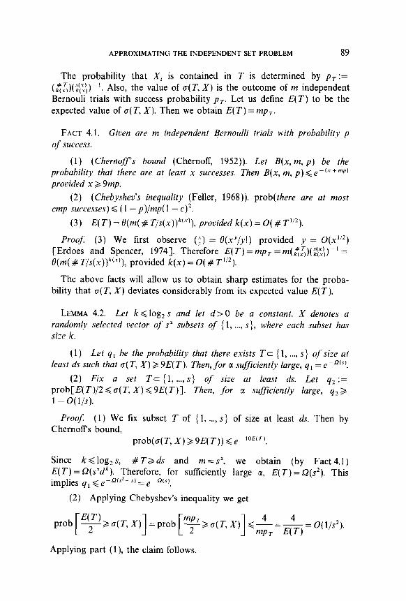
The probability that Xi is contained in T is determined by pT := (z.:)($\))‘. Also, the value of a( T, X) is the outcome of m independent Bernouli trials with success probability pT. Let us define E(T) to be the expected value of a( T, X). Then we obtain E(T) = mp,.

FACT 4.1. Given are m independent Bernoulli trials u?th probability p of success.

(1) (Chernoffs bound (Chernoff, 1952)). Let B(x, m, p) be the probability that there are at least x successes. Then B(x, m, p) < e-(x+mP) provided x 2 9mp.

(2) (Chebyshev’s inequality (Feller, 1968)). prob(there are at most cmp successes)d(l-p)/mp(l-c)‘.

(3) E(T) = 0(m( # T/s(x))~‘~‘), provided k(x) = 0( # T1j2).

Proof: (3) We first observe (;) = 0(x-“/y!) provided y = O(x’12) [Erdoes and Spencer, 19741. Therefore E(T) = mp, = m( ~.rT;)($$-’ = t9(m( # T/s(x))“‘-“), provided k(x) = 0( # T’12).

The above facts will allow us to obtain sharp estimates for the probability that r~( T, X) deviates considerably from its expected value E(T).

LEMMA 4.2. Let k < log, s and let d> 0 be a constant. X denotes a randomly selected vector of sa subsets of (1, . . . . s}, where each subset has size k.

(1) Let q, be the probability that there exists Tc { 1, . . . . s} of size at least ds such that a( T, X) > 9E( T). Then, for u sufficiently large, q, = ee*@).

(2) Fix a set Tc { 1, . . . . s} of size at least ds. Let q2 := prob[E( T)/2 < a( T, X) 6 9E( T)]. Then, for c( sufficiently large, q2 > 1 - O( l/s).

Proof: (1) We fix subset T of { 1, . . . . s} of size at least ds. Then by Chernoff’s bound,

prob(o( T, X) > 9E( T)) d e- 1oE(T’.

Since k 6 log, s, # T3 ds and m = sa, we obtain (by Fact 4.1) E(T) = SZ(s”d’). Therefore, for sufficiently large c(, E(T) = Q(s2). This implies q1 f e 4?(s~--s)=,-m)

(2) Applying Chebyshev’s inequality we get

->a(T, X) =prob 1 [ +T(,.) &z-E 1 4 mp, E(T) o(1’s2)’

Applying part (1 ), the claim follows,


Now we have all the tools to finally investigate the transformation from a nice maximization problem (& P) to (Fk, P).

LEMMA 4.3. Let (F, P) be a c-nice maximization problem for a positive constant c. We also demand that (F, P) possesses an approximation algorithm of constant quality. Let k be a polynomial time computable function with k(x) < logz(s(x)). Then

(F, f’) <a (F/c, PI where A(q,x)= [O(q+ l)]““‘“‘- 1.

In particular, if (F, P) cannot be approximated in random polynomial time with quality < E, then it is impossible to approximate (Fk, P) in random polynomial time with quality = 0( (1 + E)‘(-~’ ) (provided k(x) < log,(s(x))).

Proof: Let x be an instance of the c-nice maximization problem (F, P). Randomly generate m = s(x)’ subsets X,, . . . . X, of ( 1, . . . . s(x)> of size

k(x). Fix CI so that Lemma 4.2 can be applied for d= c/2. Remember that Fk(y, X) is equal to the sum of those multinomials of F( Y)~‘“’ that are specified by X= (X, , . . . . X,).

Next choose some optimal solution ymax for (F, P). Let T= (i: y max i = 11. f’,(~rn,x, X) equals the number of all subsets Xi that are contained in T, since the “products” of all other sets evaluate to 0. According to the previous lemma, we will find (with probability 1 -0(1/s(x))) at least E(T)/2 such subsets. Therefore (with high probability) E( T)/2 < Fk(ymax, X) and thus opt&x, X) > E( T)/2 (with high probability).

Our next goal is to show opt,,.(x)= 0(&T)). This will establish opt&x) = 8(E( T)). Consider a feasible solution z,,, of (F, P) such that ( z,,,, X) is an optimal solution of (Fk, P). Then zmax induces canonically a subset Tk of { 1, . . . . s(x)}. Obviously, optFk.P (x, X) is the number of sets Xi contained in Tk.

Case 1. #T,< #T/2. Insert new elements into T,, so that its size will be #T/2 (and therefore of size at least cs/2). Now we can apply Lemma 4.2 and obtain F&ma, 2 X) 6 9E( T) with exponentially small failure probability. Thus oPtF,,.(x, m = O(E(T)).

Case 2. # Tk 2 # T/2. We obtain, with exponentially small failure probability, opt,,,.(x, X) d 9E(T,). But we also have E(T,) 6 E(T). Thus we have again opt,&, X) = O(E(T)).

We now have to define the transformation that maps feasible solutions of (Fkk, P) to feasible solutions of (F, P). Let (z, X) be a feasible solution approximating opt,,,, with quality q. In other words,


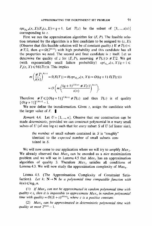
opt&x, X)/F,(z, X) = q+ 1. Let T(z) be the subset of { 1, . . . . s(x)} corresponding to z.

First we run the approximation algorithm for (F, P). The feasible solution returned by the algorithm is a first candidate to be assigned to (z, X). (Observe that this feasible solution will be of constant quality.) If # T(z) < # T/2, then q = Q(2k’“‘) with high probability and this candidate has all the properties we need. The second and final candidate is 2 itself. Let us determine the quality of z for (P’, P), assuming # T(z) > # T/2. We get (with exponentially small failure probability) opt,,.(,~, X)/q + 1 6 Fk(z, X) < 9E( T(z)). This implies

= QE(T)) = NoP~,,,,(x, J3) = O((q + 1) E(T(z)))

(q+ l)“k’“’ #T(z)

s(x)

Therefore # Tg [O(q + l)]l’k(x) # T(z) and thus T(z) is of quality [O(q+ l)]“k’“‘- 1.

We now define the transformation. Given Z, assign the candidate with the larger value of F. 1

Remark 4.4. Let U= { 1, . . . . PZ}. Observe that our construction can be made deterministic, provided we can construct polynomial in n many small substs of U (of size log n) such that for eoery subset S of U (of linear size),

the number of small subsets contained in S is “roughly” identical to the expected number of small subsets contained in S.

We will now come to our application where we will try to amplify Max,. We already observed that Max, can be encoded as a nice maximization problem and we will see in Lemma 4.5 that Max, has an approximation algorithm of quality 3. Therefore Max, satisfies all conditions of Lemma 4.3. We will now study the approximation complexity of Max&.

LEMMA 4.5. (The Approximation Complexity of Constraint Satis- faction). Let k: N + N be a polynomial time computable function with k(n) <log, n.

(1) If Max, can not be approximated in random polynomial time with quality < E, then it is impossible to approximate Max, in random polynomial time with quality = 0( ( 1 + E)~~(~) ), where c is a positive constant.

(2) Max, can be approximated in deterministic polynomial time with quality at most 2k(“‘- 1.


ProoJ: (1) follows directly from Lemma 4.3 and our previous observa- tion that the instances of the randomized kth power of Max? (in the sense of Definition 4.2) are instances of Maxzk. The constant c has to be introduced since the reduction of MaxI to Max, increases the number of variables by a polynomial.

(2) We describe an approximation algorithm for Max, (assuming k(n) <log, n), generalizing Johnson’s approximation (Johnson, 1974). Let x , , . . . . x, be the variables of an instance c1 of Max,.

Preprocessing. Remove all unsatisfiable constraints and assign weight 1 to all (say) m remaining constraints.

The ith Iteration. Assume that truth values have already been assigned to {x, ) . ..) x ,~ , ). Let MI,, be the total weight of all constraints that are falsified when setting .yi = h.

Case 1. M’()>w,. Set xi = 1. Let cl, . . . . L’, be all the constraints that utould be falisified when setting x1 = 0. Remove the weight from all constraints that are now falsified and redistribute their total weight ull over c,, . . . . c,. According to our case assumption this can be achieved with no constraint more than doubling its previous weight.

Case 2. wO < w , . Set x, = 0 and distribute the weight w0 accordingly.

Observe that no constraint receives a weight larger than 2“‘“‘. Since any constraint of non-zero weight is satisfied by our truth assignment, we will have satisfied at least m/2k’“’ constraints. 1

We conclude this section with applications for Independent Set and Longest Common Subsequence (Garey and Johnson, 1979, a problem with important applications in computational molecular genetics).

THEOREM 4.6. (1) Max 2Sat < Max,. Therefore, a randomized PTAS for Max, implies the existence qf a randomized PTAS for Max 2Sat.

(2) Maxlog ,, < Independent Set.

(3) Independent Set < Longest Common Subsequence.

(4) Assume that Max 2Sat does not have a randomized PTAS. Then there is a positive constant c such that neither Independent Set nor Longest Common Subsequence possesses pol.ynomial time approximation algorithms of quality n’.

Proof: Parts (1) and (2) are standard. (3) follows from (Maier, 1978). (4) is a direct consequence of (2) and (3) in combination with Lemma 4.5.


5. CONCLUSIONS AND OPEN PROBLEMS

We have defined reducibilities which preserve the quality of approximation algorithms producing feasible solutions, and we presented complete problems.

We were able to derive negative results concerning the existence of approximation algorithms for specific problems (like Independent Set). This was achieved by considering Maximum 2-Satisfiability. We extended Maxi- mum 2-Satisfiabifity into a hierarchy of Constraint Satisfaction problems and showed that their approximation complexity critically depends on the number of variables per constraint. Since any of our Constraint Satisfaction problems can be canonically reduced to the Independent Set problem, our negative result for Independent Set followed.

We conjecture that the degree of Independent Set is incomplete. (This could explain why previous attempts failed in obtaining strong evidence against the existence of efficient algorithms with “good” approximation behavior.) Therefore we considered whether structural constraints of the feasible domain prevent completeness. We were able to show that complete functions exist whose feasibility domain is monotone. On the other hand, we conjecture that optimization problems are incomplete whenever their feasibility predicate is described by a monotone circuit (provided their objective function is sufficiently “easy”). In the introduction, we mentioned the Monotone Circuit problem as an example.

It seems that the degrees of many important optimization problems are incomparable. Correspondingly one could relax the reducibility 6, for instance allowing a polylogarithmic decrease in quality and allowing Turing reductions. Following these ideas, it is possible to reduce Chromatic Number to Independent Set (Johnson, 1974, pp. 275). Also, functions based on NP-complete languages (see the beginning of Chap. 3) become complete under Turing reductions. This is desirable, since strong negative results on the approximation complexity already follow for any function which is complete under these stronger reductions.

ACKNOWLEDGMENT

We would thank Howard Karloff and Mark Krentel for helpful discussions

RECEIVED December 16, 1988; FINAL MANUSCRIPT RECEIVED December 27. 1989


REFERENCES

AUSIELLO, G., D’ATRI, A.. AND PROTASSI, M.. (1977), On the structure of combinatorial problems and structure preserving reductions, in “Proc. 4th Intl. Coll. on Automata, Languages and Programming,” pp. 45-57.

AUSIELLO, G., D’ATRI. A., AND PROTASSI, M. (1980), Structure preserving reductions among convex optimization problems, J. Compuf. System Sci. 21, 136.

AUSIELLO, G., MARCHETTI~PACCAMELA, A., AND PROTASSI, M. (1980), Towards a unilied approach for the classification of NP-complete optimization problems, Theoret. Compuf. Sci. 12, 83.

CHERNOFF. H. (1952), A measure of asymptotic efficiency for tests of a hypothesis based on the sum of observations, Ann. of Math. Statist. 23, 493.

ERDOES, P., AND SPENCER, J. (1974), “Probabilistic Methods in Combinatorics,” Academic Press, San Diego.

FELLER, W. (1968), “An Introduction to Probability Theory and its Applications,” Vol. 1, 3rd ed., Wiley, New York.

GAREY, M. R., AND JOHNSON, D. S. (1979), “Computers and Intractability: A Guide to the Theory of NP-Completeness,” Freeman, San Francisco.

JOHNSON, D. S. (1974), Approximation algorithms for combinatorial problems, J. Cornpur. System Sci. 9, 256.

KRENTEL, M. W. (1986), The complexity of optimization problems,” in “Proc. 18th Annual ACM Symp. on Theory of Computing,” pp. 69-76.

LEIGHTON, T., AND RAO, S. (1988), An approximate max-flow min-cut theorem for uniform multicommodity flow problems with applications to approximate algorithms, in “Proc. 29th Annual Symp. on Foundations of Computer Science,” pp. 422431.

MAIER. D. (1978), The complexity of some problems on subsequences and supersequences, J. Assoc. Comput. Mach. 25, 322.

MEHLHORN, K. (1984), “Data Structures and Algorithms Two: Graph Algorithms and NP-Completeness,” pp. 183-184, EATCS Monographs on Theoretical Computer Science, Springer-Verlag, Berlin/New York.

NIVEN, I. M., AND ZUCKERMAN, H. S. (1980), “An Introduction to the Theory of Numbers,” pp. 224225, Wiley, New York.

ORPONEN, P., AND MANNILA, H. (1987), “On Approximation Preserving Reductions: Complete Problems and Robust Measures,” Technical Report, University of Helsinki.

PAZ, A., AND MORAN, S. (1981), Non deterministic polynomial optimization problems and their approximation, Theoref. Comput. Sci. 15, 251.

PAPADIMITRIOU, C. H., AND YANNAKAKIS, M. (1988), Optimization, approximation and complexity classes, in “Proc. 20th Annual ACM Symp. on Theory of Computing,” pp. 229-234.

ROBERTS, F. S. (1984), “Applied Combinatorics,” pp. 212-213, Prentice-Hall, Englewood Cliffs, N.J.

SIMON, H. U. (1988), “On Approximate Solutions for Combinatorial Optimization Problems,” Technical Report 15/1988. Sonderforschungsbereich 124, Universitaet Saarbruecken.

on the complexity of approximating the independent set

Documents