on the communication and streaming complexity of...
TRANSCRIPT
On the communication and streaming complexity of maximum
bipartite matching
Ashish Goel
⇤Michael Kapralov
†Sanjeev Khanna
‡
November 27, 2011
AbstractConsider the following communication problem. Alice holdsa graph GA = (P,Q,EA) and Bob holds a graph GB =(P,Q,EB), where |P | = |Q| = n. Alice is allowed tosend Bob a message m that depends only on the graphGA. Bob must then output a matching M ✓ EA [EB . What is the minimum message size of the messagem that Alice sends to Bob that allows Bob to recovera matching of size at least (1 � ✏) times the maximummatching in GA [ GB? The minimum message length isthe one-round communication complexity of approximatingbipartite matching. It is easy to see that the one-roundcommunication complexity also gives a lower bound on thespace needed by a one-pass streaming algorithm to computea (1� ✏)-approximate bipartite matching. The focus of thiswork is to understand one-round communication complexityand one-pass streaming complexity of maximum bipartitematching. In particular, how well can one approximate theseproblems with linear communication and space? Prior toour work, only a 1
2
-approximation was known for both theseproblems.
In order to study these questions, we introduce theconcept of an ✏-matching cover of a bipartite graph G, whichis a sparse subgraph of the original graph that preserves thesize of maximum matching between every subset of verticesto within an additive ✏n error. We give a polynomial timeconstruction of a 1
2
-matching cover of size O(n) with somecrucial additional properties, thereby showing that Aliceand Bob can achieve a 2
3
-approximation with a messageof size O(n). While we do not provide bounds on thesize of ✏-matching covers for ✏ < 1/2, we prove that ingeneral, the size of the smallest ✏-matching cover of agraph G on n vertices is essentially equal to the size ofthe largest so-called ✏-Ruzsa Szemeredi graph on n vertices.We use this connection to show that for any � > 0, a( 23
+�)-approximation requires a communication complexity
of n1+⌦(1/ log logn).
⇤Departments of Management Science and Engineering and
(by courtesy) Computer Science, Stanford University. Email:
[email protected]. Research supported in part by NSF
award IIS-0904325.
†Institute for Computational and Mathematical Engineering,
Stanford University. Email: [email protected]. Research
supported in part by NSF award IIS-0904325 and a Stanford
Graduate Fellowship.
‡Department of Computer and Information Science,
University of Pennsylvania, Philadelphia PA. Email:
[email protected]. Supported in part by NSF Awards
CCF-1116961 and IIS-0904314.
We also consider the natural restrictingon of the prob-lem in which GA and GB are only allowed to share verticeson one side of the bipartition, which is motivated by appli-cations to one-pass streaming with vertex arrivals. We showthat a 3
4
-approximation can be achieved with a linear sizemessage in this case, and this result is best possible in thatsuper-linear space is needed to achieve any better approxi-mation.
Finally, we build on our techniques for the restricted
version above to design one-pass streaming algorithm for the
case when vertices on one side are known in advance, and
the vertices on the other side arrive in a streaming manner
together with all their incident edges. This is precisely the
setting of the celebrated (1 � 1
e )-competitive randomized
algorithm of Karp-Vazirani-Vazirani (KVV) for the online
bipartite matching problem [12]. We present here the
first deterministic one-pass streaming (1� 1
e )-approximation
algorithm using O(n) space for this setting.
1 Introduction
We study the communication and streaming complex-ity of the maximum bipartite matching problem. Con-sider the following scenario. Alice holds a graph GA =(P,Q,EA) and Bob holds a graph GB = (P,Q,EB),where |P | = |Q| = n. Alice is allowed to send Bob amessage m that depends only on the graph GA. Bobmust then output a matching M ✓ EA [ EB . What isthe minimum size of the message m that Alice sends toBob that allows Bob to recover a matching of size atleast 1� ✏ of the maximum matching in GA [GB? Theminimum message length is the one-round communi-cation complexity of approximating bipartite matching,and is denoted by CC(✏, n). It is easy to see that thequantity CC(✏, n) also gives a lower bound on the spaceneeded by a one-pass streaming algorithm to computea (1 � ✏)-approximate bipartite matching. To see this,consider the graph GA [ GB revealed in a streamingmanner with edge set EA revealed first (in some arbi-trary order), followed by the edge set EB . It is clear thatany non-trivial approximation to the bipartite matchingproblem requires ⌦(n) communication and ⌦(n) space,respectively, for the one–round communication and one-
pass streaming problems described above. The centralquestion considered in this work is how well can we ap-proximate the bipartite matching problem when onlyO(n) communication/space is allowed.
Matching Covers: We show that a study of thesequestions is intimately connected to existence of sparse“matching covers” for bipartite graphs. An ✏-matchingcover or simply an ✏-cover, of a graph G(P,Q,E) isa subgraph G0(P,Q,E0) such that for any pairs ofsets A ✓ P and B ✓ Q, the graph G0 preservesthe size of the largest A to B matching to withinan additive error of ✏n. The notion of matchingsparsifiers may be viewed as a natural analog of thenotion of cut-preserving sparsifiers which have playeda very important role in the study of network designand connectivity problems [11, 4]. It is easy to seethat if there exists an ✏-cover of size f(✏, n) for somefunction f , then Alice can just send a message ofsize f(✏, n) to allow Bob to compute an additive ✏nerror approximation to bipartite matching (and (1� ✏)-approximation whenever GA [ GB contains a perfectmatching). However, we show that the question ofconstructing e�cient ✏-covers is essentially equivalent toresolving a long-standing problem on a family of graphsknown as the Ruzsa-Szemeredi graphs. A bipartitegraph G(P,Q,E) is an ✏-Ruzsa-Szemeredi graph if Ecan be partitioned into a collection of induced matchingsof size at least ✏n each. Ruzsa-Szemeredi graphshave been extensively studied as they arise naturallyin property testing, PCP constructions and additivecombinatorics [7, 10, 17]. A major open problem isto determine the maximum number of edges possiblein an ✏-Ruzsa-Szemeredi graph. In particular, do thereexist dense graphs with large locally sparse regions (i.e.large induced subgraphs are perfect matchings)? Weestablish the following somewhat surprising relationshipbetween matching covers and Ruzsa-Szemeredi graphs:for any ✏ > 0 the smallest possible size of an ✏-matchingcover is essentially equal to the largest possible numberof edges in an ✏-Ruzsa-Szemeredi graph.
Constructing dense ✏-Ruzsa-Szemeredi graphs forgeneral ✏ and proving upper bounds on their size ap-pears to be a di�cult problem [9]. To our knowl-edge, there are two known constructions in the liter-ature. The original construction due to Ruzsa andSzemeredi yields a collection of n/3 induced matchingsof size n/2O(
plogn) using Behrend’s construction of a
large subset of {1, . . . , n} without three-term arithmeticprogressions [3, 17]. Constructions of a collection ofnc/ log logn induced matchings of size n/3 � o(n) weregiven in [7, 15]. We use the ideas of [7, 15] to construct( 12
� �)-Ruzsa-Szemeredi graphs with n1+⌦�(1/ log logn)
edges and a more general construction for the vertex ar-
rival case. To the best of our knowledge, the only knownupper bound on the size of ✏-Ruzsa-Szemeredi graphsfor constant ✏ < 1
2
is O(n2/ log⇤ n) that follows fromthe bound used in an elementary proof of Roth’s theo-rem [17].
One-round Communication: We show that in factCC(✏, n) 2n � 1 for all ✏ � 1
3
, i.e. a messageof linear size su�ces to get a 2
3
-approximation to themaximum matching in GA [ GB . We establish thisresult by constructing an O(n) size 1
2
-cover of the inputgraph that satisfies certain additional properties whichallows Bob to recover a 2
3
-approximation1. We referto this particular 1
2
-cover as a matching skeleton ofthe input graph, and give a polynomial time algorithmfor constructing it. Next, building on the above-mentioned connection between matching covers andRuzsa-Szemeredi graphs, we show the following tworesults: (a) our construction of 1
2
-cover implies thatfor any � > 0, there do not exist ( 1
2
+ �)-Ruzsa-Szemeredi graph with more than O(n/�) edges, and(b) our 2
3
-approximation result is best possible whenonly linear amount of communication is allowed. Inparticular, Alice needs to send n1+⌦(1/ log logn) bits toachieve a ( 2
3
+�)-approximation, for any constant � > 0,even when randomization is allowed.
We then study the one round communication com-plexity CCv(✏, n) of (1 � ✏)-approximate maximummatching in the restricted model when the graphs GA
and GB are only allowed to share vertices on one side ofthe bipartition. This model is motivated by applicationto one-pass streaming computations when the verticesof the graph arrive together with all incident edges. Weobtain a stronger approximation result in this model,namely, using the preceding 1
2
-cover construction weshow that CCv(✏, n) 2n � 1 for ✏ � 1/4. Thus a3
4
-approximation can be obtained with linear communi-cation complexity, and as before, we show that obtain-ing a better approximation requires a communicationcomplexity of n1+⌦(1/ log logn) bits.
One-pass Streaming: We build on our techniques forone-round communication to design a one-pass stream-ing algorithm for the case when vertices on one sideare known in advance, and the vertices on the otherside arrive in a streaming manner together with alltheir incident edges. This is precisely the setting ofthe celebrated (1 � 1
e )-competitive randomized algo-rithm of Karp-Vazirani-Vazirani (KVV) for the onlinebipartite matching problem [12]. We give a determin-istic one-pass streaming algorithm that matches the(1 � 1
e )-approximation guarantee of KVV using only
1
We note here that a maximum matching in a graph is only a
2
3
-cover.
O(n) space. Prior to our work, the only known deter-ministic algorithm for matching in one-pass streamingmodel, even under the assumption that vertices arrivetogether with all their edges, is the trivial algorithmthat keeps a maximal matching, achieving a factor of1
2
. We note that in the online setting, randomization iscrucial as no deterministic online algorithm can achievea competitive ratio better than 1
2
.
Related work: The streaming complexity of maxi-mum bipartite matching has received significant atten-tion recently. Space-e�cient algorithms for approximat-ing maximum matchings to factor (1�✏) in a number ofpasses that only depends on 1/✏ have been developed.The work of [14] gave the first space-e�cient algorithmfor finding matchings in general (non-bipartite) graphsthat required a number of passes dependent only on1/✏, although the dependence was exponential. Thisdependence was improved to polynomial in [5], where(1� ✏)-approximation was obtain in O(1/✏8) passes. Ina recent work, [2] obtained a significant improvement,achieving (1 � ✏)-approximation in O(log log(1/✏)/✏2)passes (their techniques also yield improvements for theweighted version of the problem). Further improve-ments for the non-bipartite version of the problem havebeen obtained in [1]. Despite the large body of workon the problem, the only known algorithm for one passis the trivial algorithm that keeps a maximal matching.No non-trivial lower bounds on the space complexity ofobtaining constant factor approximation to maximumbipartite matching in one pass were known prior to ourwork (for exact computation, an ⌦(n2) lower bound wasshown in [6]).
Organization: We start by introducing relevant defi-nitions in section 2. In section 3 we give the construc-tion of the matching skeleton, which we use later insection 4 to prove that CC(1/3, n) = O(n), as well asshow that the matching skeleton forms a 1/2-cover. Insection 5 we deduce using the matching skeleton thatCCv(1/4, n) = O(n). In section 6 we use these tech-niques to obtain a deterministic one-pass (1� 1/e) ap-proximation to maximum matching in O(n) space inthe vertex arrival model. We extend the construction ofRuzsa-Szemeredi graphs from [7, 15] in section 7. Weuse these extensions in section 8 to show that our upperbounds on CC(✏, n) and CCv(✏, n) are best possible, aswell as to prove lower bounds on the space complexityof one-pass algorithms for approximating maximum bi-partite matching. Finally, in section 9 we prove the cor-respondence between the size of the smallest ✏-matchingcover of a graph on n nodes and the size of the largest✏-Ruzsa-Szemeredi graph on n nodes.
2 Preliminaries
We start by defining bipartite matching covers, whichare matchings-preserving graph sparsifiers.
Definition 2.1. Given an undirected bipartite graphG = (P,Q,E), and sets A ✓ P,B ✓ Q, and H ✓ E, letMH(A,B) denote the size of the largest matching in thegraph G0 = (A,B, (A⇥B) \H).
Given an undirected bipartite graph G = (P,Q,E)with |P | = |Q| = n, a set of edges H ✓ E is said to bean ✏-matching-cover of G if for all A ✓ P,B ✓ Q, wehave MH(A,B) � ME(A,B)� ✏n.
Definition 2.2. Define LC(✏, n) to be the smallestnumber m0 such that any undirected bipartite graphG = (P,Q,E) with P = Q = n has an ✏-matching-coverof size at most m0.
We next define induced matchings and Ruzsa-Szemeredi graphs.
Definition 2.3. Given an undirected bipartite graphG = (P,Q,E) and a set of edges F ✓ E, let P (F ) ✓ Pdenote the set of vertices in P which are incident on atleast one edge in F , and analogously, let Q(F ) denotethe set of vertices in Q which are incident on at leastone edge in F . Let E(F ), called the set of edges inducedby F , denote the set of edges E \ (P (F )⇥Q(F )). Notethat E(F ) may be much larger than F in general.
Given an undirected bipartite graph G = (P,Q,E),a set of edges F ✓ E is said to be an induced matchingif no two edges in F share an endpoint, and E(F ) = F .Given an undirected bipartite graph G = (P,Q,E)and a partition F of E, the partition is said to be aninduced partition of G if every set F 2 F is an inducedmatching. An undirected bipartite graph G = (P,Q,E)with P = Q = n is said to have an ✏-induced partitionif there exists an induced partition of G such every setin the partition is of size at least ✏n. Following [7], werefer to graphs that have an ✏-induced partition as ✏-Ruzsa-Szemeredi graphs.
Definition 2.4. Let UI(✏, n) denote the largest numberm such that there exists an undirected bipartite graphG = (P,Q,E) with |E| = m, |P | = |Q| = n, and withan ✏-induced partition.
Note that for any 0 < ✏1
< ✏2
< 1, any ✏2
-inducedpartition of a graph is also an ✏
1
-induced partition,and hence, UI(✏, n) is a non-increasing function of✏. Analogously, any ✏
1
-matching-cover is also an ✏2
-matching cover, and hence, LC(✏, n) is also a non-increasing function of ✏.
3 Matching Skeletons
Let G = (P,Q,E) be a bipartite graph. We now definea subgraph G0 = (P,Q,E0) of G that contains at most(|P | + |Q| � 1) edges, and encodes useful informationabout matchings in G. We refer to this subgraph G0
as a matching skeleton of G, and this construction willserve as a building block for our algorithms. Amongother things, we will show later that G0 is a 1
2
-cover ofG.
We present the construction of G0 in two steps. Wefirst consider the case when P is hypermatchable, thatis, for every vertex v 2 Q there exists a perfect matchingof the P side that does not include v. We then extendthe construction to the general case using the Edmonds-Gallai decomposition [16].
3.1 P is hypermatchable in G We note that sinceP is hypermatchable, by Hall’s theorem [16], we havethat |�(A)| > |A| for all A ✓ P . For a parameter↵ 2 (0, 1], let RG(↵) = {A ✓ P : |�G(A)| (1/↵)|A|}.Note that as the parameter ↵ decreases, the expansionrequirement in the definition above increases. We willomit the subscript G when G is fixed, as in the nextlemma.
Lemma 3.1. Let ↵ 2 (0, 1] be such that R(↵+✏) = ; forany ✏ > 0, i.e. G supports an 1
↵+✏ -matching of the P -side for any ✏ > 0. Then for any two A
1
2 R(↵), A2
2R(↵) one has A
1
[A2
2 R(↵).
Proof. Let B1
= �(A1
) and B2
= �(A2
). First, since(A
1
⇥ (Q\B1
))\E = ; and (A2
⇥ (Q\B2
))\E = ;, wehave that (A
1
\A2
)⇥(Q\(B1
\B2
)) = ;. Furthermore,since R(↵+ ✏) = ;, one has |B
1
\B2
| � (1/↵)|A1
\A2
|.Also, we have |Bi| |Ai|/↵, i = 1, 2. Hence,
|B1
[B2
| = |B1
|+ |B2
|� |B1
\B2
| (1/↵)(|A
1
|+ |A2
|� |A1
\A2
|) = (1/↵)|A1
[A2
|,
and thus (A1
[A2
) 2 R(↵) as required.
We now define a collection of sets (Sj , Tj), j =1, . . . ,+1, where Sj ✓ P, Tj ✓ Q,Si \ Sj = ;, i 6= j.
1. Set j := 1, G0
:= G,↵0
:= 1. We have RG0(↵0
) =;.
2. Let � < ↵j�1
be the largest real such thatRGj�1(�) 6= ;.
3. Let S� =S
A2R(�) A, and T� = �(S�). We haveS� 2 RRj�1(�) by Lemma 3.1.
4. Let Gj := Gj�1
\ (S� [ T�). We refer to thevalue of ↵ at which a pair (S↵, T↵) gets removed
from the graph as the expansion of the pair. SetSj := S� , Tj := T� ,↵j := �. IfGj 6= ;, let j := j+1and go to (2).
The following lemma is an easy consequence of theabove construction.
Lemma 3.2. 1. For each U ✓ Sj one has |�Gj (U)| �(1/↵j)|U |.
2. For every k > 0,
0
@
0
@[
jk
Sj
1
A⇥
0
@Q \[
jk
Tj
1
A
1
A \ E = ;.
Proof. We prove (1) by contradiction. When j = 1, (1)follows immediately since we are choosing the largest� such that R(�) 6= ;. Otherwise suppose that thereexists U ✓ PGj such that |�Gj (U)| < (1/↵j)|U |. Thenfirst observe that |�Gj (U)| > (1/↵j�1
)|U |. If not then
|�Gj�1(Sj�1
[ U)| = |Tj�1
|+ |�Gj (U)|
1
↵j�1
(|Sj�1
|+ |U |) 1
↵j�1
(|Sj�1
[ U |),
since Sj�1
\ PGj = ; by construction. Now as↵j < ↵j�1
is chosen to be the largest real for whichthere exists some subset U 0 ✓ PGj with |�Gj (U
0)| (1/↵j)|U 0|, it follows that for every U ✓ PGj , we musthave |�Gj (U)| � (1/↵j)|U |.
(2) follows by construction.
To complete the definition of the matching skeleton,we now identify the set of edges of G that our algorithmkeeps. For a parameter � � 1 and subsets S ✓ P ,T ✓ Q we refer to a (fractional) matching M thatsaturates each vertex in S exactly � times (fractionally)and each vertex in T at most once as a �-matching ofS in (S, T, (S ⇥ T ) \ E). By Lemma 3.2 there existsa (fractional) (1/↵j)-matching of Sj in (Sj , Tj , (Sj ⇥Tj) \ E). Moreover, one can ensure that the matchingis supported on the edges of a forest by rerouting flowalong cycles. Let Mj be a fractional (1/↵j)-matching in(Sj , Tj) that is a forest.
Interestingly, the fractional matching correspondingto the matching skeleton is identical to a 1-majorizedfractional allocation of unit-sized jobs to (1 � 1) ma-chines [13, 8]; as a result, the fractional matchingsxe simultaneously minimize all convex functions of thexe’s subject to the constraint that every node in P ismatched exactly once.
3.2 General bipartite graphs We now extend theconstruction to general bipartite graphs using theEdmonds-Gallai decomposition of G(P,Q,E), which es-sentially allows us to partition the vertices of G into setsAP (G), DP (G), CP (G), AQ(G), DQ(G), and CQ(G)such that AP (G) is hypermatchable toDQ(G), AQ(G) ishypermatchable toDP (G), and there is a perfect match-ing between CP (G) and CQ(G).
The Edmonds-Gallai decomposition theorem is asfollows.
Theorem 3.1. (Edmonds-Gallai decomposition, [16])Let G = (V,E) be a graph. Then V can be partitionedinto the union of sets D(G), A(G), C(G) such that
D(G) = {v 2 V |9 a maximum matching missing v}A(G) = �(D(G))
C(G) = V \ (D(G) [A(G)).
Moreover, every maximum matching contains a perfectmatching inside C(G).
Applying Edmonds-Gallai decomposition to bipar-tite graphs, we get
Corollary 3.1. Let G = (P,Q,E) be a graph.Then V can be partitioned into the union of setsDP (G), DQ(G), AP (G), AQ(G), CP (G), CQ(G) suchthat
DP (G) = {v 2 P |9 a maximum matching missing v}DQ(G) = {v 2 Q|9 a maximum matching missing v}AP (G) = �(DQ(G))
AQ(G) = �(DP (G))
CP (G) = P \ (DP (G) [AP (G))
CQ(G) = Q \ (DQ(G) [AQ(G)).
Moreover,
1. there exists a perfect matching between CP (G) andCQ(G)
2. for every U ✓ AP (G) one has |�(U)\DQ(G)| > |U |
3. for every U ✓ AQ(G) one has |�(U) \ DP (G)| >|U |.
Proof. (1) is part of the statement of Theorem 3.1. Toshow (2), note that by definition of DQ(G) for eachvertex v 2 DQ(G) there exists a maximum matchingthat misses v. Thus, |�(U) \ DQ(G)| > |U | for everyset U .
Using the above partition, we can now define amatching skeleton of G. Let S
0
= CP (G), T0
=
CQ(G), and let M0
be a perfect matching between S0
and T0
. Let (S1
, T1
), . . ., (Sj , Tj) be the expandingpairs obtained by the construction in the previoussection on the graph induced by AP (G) [ DQ(G).Let (S�j , T�j), . . ., (S�1
, T�1
) be the expanding pairsobtained by the construction in the previous sectionfrom the Q side on the graph induced by AQ(G) [DP (G).
Definition 3.1. For a bipartite graph G = (P,Q,E)we define the matching skeleton G0 of G as the unionof pairs (Sj , Tj), j = �1, . . . ,+1, with corresponding(fractional) matchings Mj. Note that G0 contains atmost |P |+ |Q|� 1 edges.
As before, we can show the following:
Lemma 3.3. 1. For each U ✓ Sj, one has |Tj \�G0(U)| � (1/↵j)|U |.
2. For every k > 0,⇣⇣
P \S
j�k Sj
⌘⇥⇣S
j�k Tj
⌘⌘\
E = ;, and⇣⇣
Q \S
j�k Sj
⌘⇥
⇣Sj�k Tj
⌘⌘\
E = ;.
Proof. Follows by construction of G0.
We note that the formulation of property (2) inLemma 3.3 is slightly di↵erent from property (2) inLemma 3.2. However, one can see that these formu-lations are equivalent when there are no (Sj , Tj) pairsfor negative j, as is the case in Lemma 3.2.
4 O(n) communication protocol for CC( 13
, n)
In this section, we prove that for any two bipartitegraphs G
1
, G2
, the maximum matching in the graphG0
1
[ G2
is at least 2/3 of the maximum matching inG
1
[ G2
, where G01
is the matching skeleton of G1
.Thus, CC(✏, n) = O(n) for all ✏ � 1/3; Alice sends thematching skeleton G0
A of her graph, and Bob computesa maximum matching in the graph G0
A [GB .Before proceeding, we establish some notation used
for the next several sections. Denote by (Sj , Tj), j =�1, . . . ,+1 the set of pairs from the definition of G0.Recall that Sj ✓ P when j � 0 and Sj ✓ Q when j < 0.Also, given a maximummatchingM in a bipartite graphG = (P,Q,E), a saturating cut corresponding to Mis a pair of disjoint sets (A
1
[ B1
, A2
[ B2
) such thatA
1
[ A2
= P,B1
[ B2
= Q, all vertices in A2
[ B1
arematched by M , there are no matching edges betweenA
2
and B1
, and no edges at all between A1
and B2
.The existence of a saturating cut follows from the max-flow min-cut theorem. Let ALG denote the size of themaximum matching in G0
1
[G2
and let OPT denote thesize of the maximum matching in G
1
[G2
.
!"# $%"#
&%"#
'%"#&"# !"# '%"#
'"#$"# !%"#!%"#'"#
("#
)*#
(*#
)"#
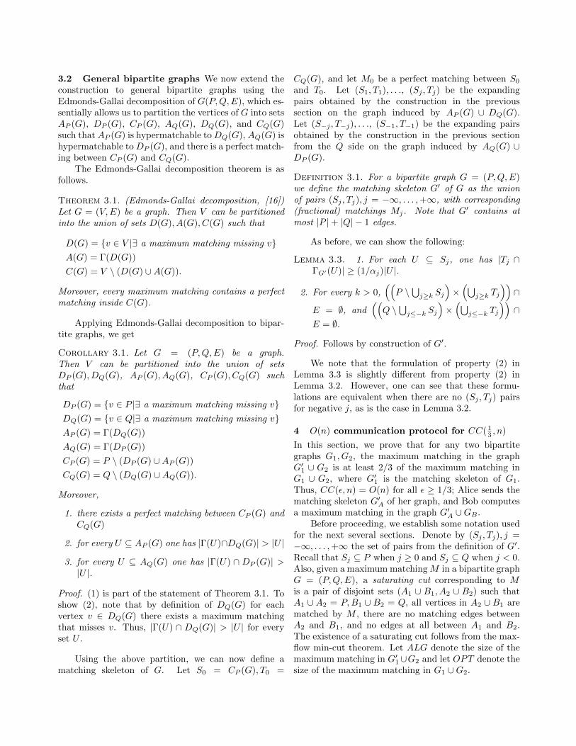
Figure 1: Distribution of (Sj , Tj) pairs across the cut
Consider a maximum matching M in (G01
[ G2
)and a corresponding saturating cut (A
1
[B1
, A2
[B2
);note that ALG = |B
1
| + |A2
|. Let M⇤ be a maximummatching in E
1
\ (A1
⇥B2
). Note that we have OPT |B
1
|+ |A2
|+ |M⇤|.We start by describing the intuition behind the
proof. Suppose for simplicity that the matching skeletonG0
1
of G1
consists of only one (Sj , Tj) pair for somej � 0, such that |Tj | = (1/↵j)|Sj |. We first notethat since the matching M⇤ is not part of the matchingskeleton, it must be that edges of M⇤ go from Sj to Tj .We will abuse notation slightly by writing M⇤ \ X todenote, for X ✓ P [ Q, the subset of nodes of X thatare matched by M⇤. Since all edges of M⇤ go from Sj toTj , we have M⇤\A
1
✓ Sj \A1
and M⇤\B2
✓ Tj \B2
.This allows us to obtain a lower bound on |B
1
| and |A2
|in terms of |M⇤| if we lower bound |B
1
| and |A2
| interms of |Sj \ A
1
| and |Tj \ B2
| respectively. First, wehave that |B
1
| � |�G01(Sj \ A
1
)| � (1/↵j)|Sj \ A1
| �(1/↵j)|M⇤|, where we used the fact that the saturatingcut is empty in G0
1
[ G2
and Lemma 3.3 . Next, weprove that |�G0
1(Sj \ A
2
) \ B2
| (1/↵j)|Sj \ A2
| (thisis proved in Lemma 4.2 below). This, together with thefact that M⇤ \ B
2
✓ Tj \ B2
= �G01(Sj \ A
2
) \ B2
,implies that |A
2
| � ↵j |M⇤|. Thus, we always have|A
2
| + |B1
| � (↵j + 1/↵j)|M⇤|, and hence the worstcase happens at ↵j = 1, i.e. when the matching skeletonG0
1
of G1
consists of only the (S0
, T0
) pair, yielding a2/3 approximation. The proof sketch that we just gaveapplies when the matching skeleton only contains onepair (Sj , Tj). In the general case, we use Lemma 3.3 tocontrol the distribution of M⇤ among di↵erent (Sj , Tj)pairs. More precisely, we use the fact that edges of M⇤
may go from Sj \ A1
to Ti \ B2
only if i j. Anotheraspect that adds complications to the formal proof isthe presence of (Sj , Tj) pairs for negative j.
!"#$ %&'$
%"#$
('$)"#$ ('$ (#$
("#$!'$("#$
*#$
+&$
*&$
+#$
%,$
),$%#'$ !'$
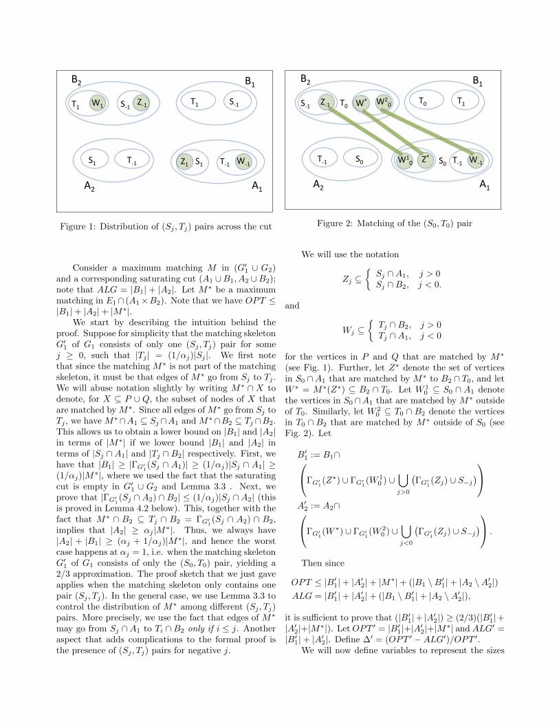
Figure 2: Matching of the (S0
, T0
) pair
We will use the notation
Zj ✓⇢
Sj \A1
, j > 0Sj \B
2
, j < 0.
and
Wj ✓⇢
Tj \B2
, j > 0Tj \A
1
, j < 0
for the vertices in P and Q that are matched by M⇤
(see Fig. 1). Further, let Z⇤ denote the set of verticesin S
0
\A1
that are matched by M⇤ to B2
\ T0
, and letW ⇤ = M⇤(Z⇤) ✓ B
2
\ T0
. Let W 1
0
✓ S0
\ A1
denotethe vertices in S
0
\A1
that are matched by M⇤ outsideof T
0
. Similarly, let W 2
0
✓ T0
\ B2
denote the verticesin T
0
\ B2
that are matched by M⇤ outside of S0
(seeFig. 2). Let
B01
:= B1
\0
@�G01(Z⇤) [ �G0
1(W 1
0
) [[
j>0
��G0
1(Zj) [ S�j
�1
A
A02
:= A2
\0
@�G01(W ⇤) [ �G0
1(W 2
0
) [[
j<0
��G0
1(Zj) [ S�j
�1
A .
Then since
OPT |B01
|+ |A02
|+ |M⇤|+ (|B1
\B01
|+ |A2
\A02
|)ALG = |B0
1
|+ |A02
|+ (|B1
\B01
|+ |A2
\A02
|),
it is su�cient to prove that (|B01
|+ |A02
|) � (2/3)(|B01
|+|A0
2
|+|M⇤|). LetOPT 0 = |B01
|+|A02
|+|M⇤| and ALG0 =|B0
1
|+ |A02
|. Define �0 = (OPT 0 �ALG0)/OPT 0.We will now define variables to represent the sizes
of the sets used in defining B01
, A02
:
w1
0
= |W 1
0
|, w2
0
= |W 2
0
|,z⇤ = |Z⇤|, w⇤ = |W ⇤|, (Note that z⇤ = w⇤)
zj = |Zj |, wj = |Wj |, rj = |�G01(Zj)|,
sj =
⇢|Sj \A
2
| j > 0|Sj \B
1
| j < 0
Lemma 4.1 expresses the size of B01
and A02
in termsof the new variables defined above.
Lemma 4.1. ALG0 =P
j 6=0
(sj+rj)+(z⇤+w1
0
)+(w⇤+
w2
0
), and OPT 0 z⇤+(z⇤+w1
0
)+(w⇤+w2
0
)+P
j 6=0
(sj+zj + rj).
Proof. The main idea is that most of the sets in thedefinitions of B0
1
and A02
are disjoint, allowing us torepresent sizes of unions of these sets by sums of sizesof individual sets.
For ALG0, recall that �G01(Sj) = Tj and hence,
the sets �G01(Sj) are all disjoint. Further, the sets Sj
are all disjoint, by construction, and disjoint with allthe Tj ’s. Thus, |A0
1
| + |B02
| = |�G01(W ⇤) [ �G0
1(W 2
0
)| +|�G0
1(Z⇤) [ �G0
1(W 1
0
)| +P
j 6=0
(sj + rj). The sets W ⇤
and W 2
0
are disjoint. Further, they are subsets of T0
(corresponding to ↵ = 1), and hence nodes in thesesets have a single unique neighbor in G0
1
; consequently|�G0
1(W ⇤)[�G0
1(W 2
0
)| = w⇤+w2
0
. Similarly, |�G01(Z⇤)[
�G01(W 1
0
)| = z⇤ + w1
0
. This completes the proof of thelemma for ALG0.
We have OPT 0 = ALG0 + |M⇤|. Consider any edge(u, v) 2 M⇤. This edge is not in G0
1
and hence must gofrom an Sj to a Tj0 where 0 j0 j or 0 � j0 � j.The number of edges in M⇤ that go from S
0
to T0
is precisely z⇤ by definition; the number of remainingedges is precisely
Pj 6=0
zj .
We now derive linear constraints on the size vari-ables, leading to a simple linear program. We have byLemma 3.3 that for all k > 0
0
@
0
@P \[
j�k
Zj
1
A⇥
0
@[
j�k
Wj
1
A
1
A \ E1
= ;,
0
@
0
@Q \[
j�k
Zj
1
A⇥
0
@[
j�k
Wj
1
A
1
A \ E1
= ;.
(4.1)
The existence of M⇤ together with (4.1)yields
+1X
j=k
zj �+1X
j=k
wj , 8k > 0,
�kX
j=�1zj �
�kX
j=�1wj , 8k > 0.
(4.2)
Furthermore, we have by definition of W 1
0
togetherwith (4.1)that
w1
0
X
j<0
zj �X
j<0
wj
w2
0
X
j>0
zj �X
j>0
wj .(4.3)
Also, we haveX
j<0
zj = w1
0
+X
j<0
wj
X
j>0
zj = w2
0
+X
j>0
wj .(4.4)
Next, by Lemma 3.3, we have rj � (1/↵j)zj . Wealso need
Lemma 4.2. (1) |�G01(Sj \A
2
)\B2
| (1/↵j)|Sj \A2
|for all j > 0, and (2) |�G0
1(Sj \B
1
)\A1
| (1/↵j)|Sj \B
1
| for all j < 0.
Proof. We prove (1). The proof of (2) is analogous.Suppose that |�G0
1(Sj \ A
2
) \ B2
| > (1/↵j)|Sj \ A2
|.Then using the assumption that (A
1
⇥B2
)\E0 = ;, weget
|Tj | = |Tj \B2
|+ |Tj \B1
|� |�G0
1(Sj \A
2
) \B2
|+ |�G01(Sj \A
1
)|> (1/↵j)|Sj \A
2
|+ (1/↵j)|Sj \A1
| > (1/↵j)|Sj |,
a contradiction to the definition of the matching skele-ton.
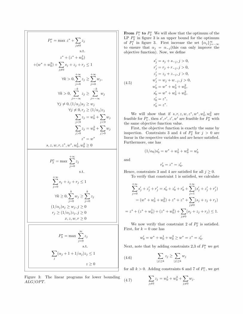
We will now bound �0 = (OPT 0 � ALG0)/OPT 0
using a sequence of linear programs, described in fig-ure 3. We will overload notation to use P ⇤
1
, P ⇤2
, P ⇤3
, re-spectively, to refer to these linear programs as well astheir optimum objective function value. By Lemma 4.2one has for all j 6= 0 that (1/↵j)sj � wj . We combinethis with equations 4.2, 4.3, and 4.4 to obtain the firstof our linear programs, P ⇤
1
, in figure 3. Bounding �0 isequivalent to bounding this LP (i.e. �0 P ⇤
1
). Notethat we have implicitly rescaled the variables so thatOPT 0 1.
We now symmetrize the LP P ⇤1
by collecting thevariables for cases when j is positive, negative, and 0 toobtain LP P ⇤
2
in figure 3. Finally, we relax LP P ⇤2
bycombining the second and third constraints, and thenestablish that the remaining constraints are all tight.This gives us the LP P ⇤
3
in figure 3. Details of theconstruction are embedded in the proof of the followinglemma.
Lemma 4.3. P ⇤1
P ⇤2
P ⇤3
.
P ⇤1
= max z⇤ +X
j 6=0
zj
s.t.
z⇤ + (z⇤ + w1
0
)
+(w⇤ + w2
0
) +X
j 6=0
sj + zj + rj 1
8k > 0,+1X
j=k
zj �+1X
j=k
wj ,
8k > 0,�kX
j=�1zj �
�kX
j=�1wj
8j 6= 0, (1/↵j)sj � wj
8j 6= 0, rj � (1/↵j)zjX
j<0
zj = w1
0
+X
j<0
wj
X
j>0
zj = w2
0
+X
j>0
wj
z⇤ = w⇤
s, z, w, r, z⇤, w⇤, w1
0
, w2
0
� 0
P ⇤2
= max+1X
j=0
zj
s.t.+1X
j=0
sj + zj + rj 1
8k � 0,kX
j=0
wj �kX
j=0
zj
(1/↵j)sj � wj , j � 0
rj � (1/↵j)zj , j � 0
x, z, w, r � 0
P ⇤3
= max1X
j=0
zj
s.t.X
j
(↵j + 1 + 1/↵j)zj 1
z � 0
Figure 3: The linear programs for lower boundingALG/OPT .
From P ⇤1
to P ⇤2
We will show that the optimum of theLP P ⇤
2
in figure 3 is an upper bound for the optimumof P ⇤
1
in figure 3. First increase the set {↵j}1j=�1to ensure that ↵j = ↵�j(this can only improve theobjective function). Now, we define
s0j = sj + s�j , j > 0,
r0j = rj + r�j , j > 0,
z0j = zj + z�j , j > 0,
w0j = wj + w�j , j > 0,
w00
= w⇤ + w1
0
+ w2
0
,
s00
= w⇤ + w1
0
+ w2
0
,
z00
= z⇤,
r00
= z⇤.
(4.5)
We will show that if s, r, z, w, z⇤, w⇤, w1
0
, w2
0
arefeasible for P ⇤
1
, then s0, r0, z0, w0 are feasible for P ⇤2
withthe same objective function value.
First, the objective function is exactly the same byinspection. Constraints 3 and 4 of P ⇤
2
for j > 0 arelinear in the respective variables and are hence satisfied.Furthermore, one has
(1/↵0
)s00
= w⇤ + w1
0
+ w2
0
= w00
andr00
= z⇤ = z00
.
Hence, constraints 3 and 4 are satisfied for all j � 0.To verify that constraint 1 is satisfied, we calculate
+1X
j=0
s0j + z0j + r0j = s00
+ z00
+ r00
++1X
j=1
(s0j + z0j + r0j)
= (w⇤ + w1
0
+ w2
0
) + z⇤ + z⇤ +X
j 6=0
(sj + zj + rj)
= z⇤ + (z⇤ + w1
0
) + (z⇤ + w2
0
) +X
j 6=0
(sj + zj + rj) 1.
We now verify that constraint 2 of P ⇤2
is satisfied.First, for k = 0 one has
w00
= w⇤ + w1
0
+ w2
0
� w⇤ = z⇤ = z00
.
Next, note that by adding constraints 2,3 of P ⇤1
we get
X
|j|�k
zj �X
|j|�k
wj(4.6)
for all k > 0. Adding constraints 6 and 7 of P ⇤1
, we get
X
j 6=0
zj = w1
0
+ w2
0
+X
j 6=0
wj .(4.7)
Subtracting (4.7) from (4.6), we get
kX
|j|=1
zj w1
0
+ w2
0
+kX
|j|=1
wj .(4.8)
Adding z⇤ to both sides and using the fact that z00
= z⇤
and w00
= z⇤ + w1
0
+ w2
0
, we get
kX
j=0
zj kX
j=0
wj .(4.9)
This completes the proof of the first half of lemma 4.3.
From P ⇤2
to P ⇤3
We now bound P ⇤2
. First we relax theconstraints by adding constraint 3 of over j from 0 to kand adding to constraint 2:
max1X
j=0
zj
s.t.1X
j=0
sj + zj + rj 1
kX
j=0
(1/↵j)sj �kX
j=0
zj , 8k � 0
rj � (1/↵j)zj , 8j � 0
x, z, w, r � 0
(4.10)
Note that the first constraint is necessarily tight atthe optimum. Otherwise scaling all variables to makethe constraint tight increases the objective function. Wenow show that all of the constraints in the second lineof (4.10) are necessarily tight at the optimum. Indeed,
let k⇤ � 0 be the smallest such thatPk⇤
j=0
(1/↵j)sj >Pk⇤
j=0
zj . Note that one necessarily has sk⇤ > 0. Let
s0 = s� �ek⇤ + (↵k⇤+1
/↵k⇤)�ek⇤+1
,
r0 = r, z0 = z,
where ej denotes the vector of all zeros with 1 in positionj. Then
kX
j=0
(1/↵j)s0j �
kX
j=0
z0j
for all k and1X
j=0
(s0j + z0j + r0j) = 1� �(1� ↵k⇤+1
/↵k⇤).
So for su�ciently small positive � > 0 one has that
s00 = s0/(1� �(1� ↵k⇤+1
/↵k⇤))
r00 = r0/(1� �(1� ↵k⇤+1
/↵k⇤))
z00 = z0/(1� �(1� ↵k⇤+1
/↵k⇤))
form a feasible solution with a better objective functionvalue.
Thus, one hasPk
j=0
(1/↵j)sj =Pk
j=0
zj for allk � 0 and hence (1/↵j)sj = zj for all j.
Additionally, one necessarily has rj = (1/↵j)zjfor all j at optimum. Indeed, otherwise decreasing rjdoes not violate any constraint and makes constraint 1slack. Then rescaling variables to restore tightness ofconstraint 1 improves the objective function. Thus, weneed to solve
P ⇤3
= max1X
j=0
zj
s.t.X
j
(↵j + 1 + 1/↵j)zj 1
z � 0
(4.11)
But P ⇤3
is easy to analyze: there exists an optimumsolution that sets all zj to zero except for a j thatminimizes (↵j + 1 + 1/↵j). For all non-negative x,f(x) = 1 + x + 1/x is minimized when x = 1, andf(1) = 3. This gives P ⇤
3
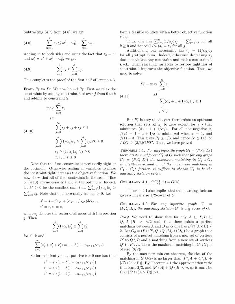
1/3, and hence �0 1/3, orALG0 � (2/3)OPT 0. Thus, we have proved
Theorem 4.1. For any bipartite graph G1
= (P,Q,E1
)there exists a subforest G0
1
of G such that for any graphG
2
= (P,Q,E2
) the maximum matching in G01
[ G2
is a 2/3-approximation of the maximum matching inG
1
[ G2
; further, it su�ces to choose G01
to be thematching skeleton of G
1
.
Corollary 4.1. CC( 13
, n) = O(n).
Theorem 4.1 also implies that the matching skeletongives a linear size 1/2-cover of G.
Corollary 4.2. For any bipartite graph G =(P,Q,E), the matching skeleton G0 is a 1
2
-cover of G.
Proof. We need to show that for any A ✓ P,B ✓Q, |A|, |B| > n/2 such that there exists a perfectmatching between A and B in G one has E0\(A⇥B) 6=;. Let G
2
= (P [P 0, Q[Q0,MP [MQ) be a graph thatconsists of a perfect matching from a new set of verticesP 0 to Q \ B and a matching from a new set of verticesQ0 to P \A. Then the maximum matching in G[G
2
isof size (3/2)n.
By the max-flow min-cut theorem, the size of thematching in G0[G
2
is no larger than |P \A|+ |Q\B|+|E0\(A⇥B)|. By Theorem 4.1 the approximation ratiois at least 2/3, and |P \A|+ |Q \B| < n, so it must bethat |E0 \ (A⇥B)| > 0.
5 O(n) communication protocol for CCv(1
4
, n)
In this section we prove that CCv(✏, n) = O(n) for all✏ < 1/4. In particular, we show that given a bipartitegraph G
1
= (P1
, Q,E1
), there exists a forest F ✓ E1
such that for any G2
= (P2
, Q,E) that may share nodeson the Q side with G
1
but not on the P side, themaximum matching in G0
1
[G2
is a 3/4-approximationof the maximum matching inG
1
[G2
. The broad outlineof the proof is similar to the previous section, but wecan now assume a special optimal matching using theassumption that G
2
may only share nodes with G1
onthe Q side. The proof uses the simple lemma below; westate it here since it is also needed in section 6.
Lemma 5.1. Let G = (P,Q,E) be a bipartite graph andlet S ✓ P be such that |�(U)| � |U | for all U ✓ S. Thenthere exists a maximum matching in G that matches allvertices of S.
The proof is quite simple: start with an arbitrarymaximum matching and repeatedly find and apply evenlength augmenting paths originating from unmatchednodes in S and going to matched nodes in P \ S, toreduce the number of unmatched nodes in S. Thesepaths exist by our condition on S. The details aredeferred to the full version of the paper.
We now state the main theorem of this section. Theproof is deferred to the full version of the paper.
Theorem 5.1. Let G1
= (P1
, Q,E1
), G2
= (P2
, Q,E2
)be bipartite graphs that share the vertex set on oneside. Let G0
1
be the matching skeleton of G1
. Then themaximum matching in G0
1
[G2
is a 3/4-approximationof the maximum matching in G
1
[G2
.
6 One-pass streaming with vertex arrivals
Let Gi = (Pi, Q,Ei) be a sequence of bipartite graphs,where Pi\Pj = ; for i 6= j. For a graph G, we denote bySPARSIFY⇤(G) the matching skeleton of G modified asfollows: for each pair (Sj , Tj), j < 0 keep an arbitrarymatching of Sj to a subset of Tj , discarding all otheredges, and collect all these matchings into the (S
0
, T0
)pair. Note that we have Sj ✓ P , where P is the side ofthe graph that arrives in the stream. We have
Lemma 6.1. Let G = (P,Q,E) be a bipartite graph. LetG0 = SPARSIFY ⇤(G). Let (Sj , Tj), j = 0, . . . ,+1denote the set of expanding pairs. Then E\(Si⇥Tj) = ;for all i < j.
Let
G01
= SPARSIFY⇤(G1
)
and
G0i = SPARSIFY⇤(G0
i�1
[Gi), i > 1
(6.12)
We will show that for each ⌧ > 0 the maximummatching in G0
⌧ is at least a 1 � 1/e fraction of themaximum matching in
S⌧i=1
Gi. We will slightly abusenotation by denoting the set of expanding pairs in G0
⌧
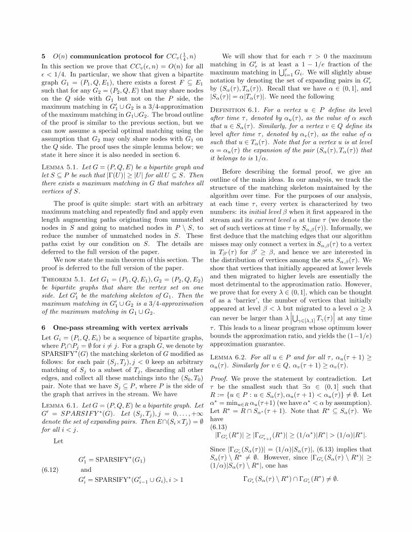
by (S↵(⌧), T↵(⌧)). Recall that we have ↵ 2 (0, 1], and|S↵(⌧)| = ↵|T↵(⌧)|. We need the following
Definition 6.1. For a vertex u 2 P define its levelafter time ⌧ , denoted by ↵u(⌧), as the value of ↵ suchthat u 2 S↵(⌧). Similarly, for a vertex v 2 Q define itslevel after time ⌧ , denoted by ↵v(⌧), as the value of ↵such that u 2 T↵(⌧). Note that for a vertex u is at level↵ = ↵u(⌧) the expansion of the pair (S↵(⌧), T↵(⌧)) thatit belongs to is 1/↵.
Before describing the formal proof, we give anoutline of the main ideas. In our analysis, we track thestructure of the matching skeleton maintained by thealgorithm over time. For the purposes of our analysis,at each time ⌧ , every vertex is characterized by twonumbers: its initial level � when it first appeared in thestream and its current level ↵ at time ⌧ (we denote theset of such vertices at time ⌧ by S↵,�(⌧)). Informally, wefirst deduce that the matching edges that our algorithmmisses may only connect a vertex in S↵,�(⌧) to a vertexin T�0(⌧) for �0 � �, and hence we are interested inthe distribution of vertices among the sets S↵,�(⌧). Weshow that vertices that initially appeared at lower levelsand then migrated to higher levels are essentially themost detrimental to the approximation ratio. However,we prove that for every � 2 (0, 1], which can be thoughtof as a ‘barrier’, the number of vertices that initiallyappeared at level � < � but migrated to a level ↵ � �
can never be larger than ����S
�2[�,1] T�(⌧)��� at any time
⌧ . This leads to a linear program whose optimum lowerbounds the approximation ratio, and yields the (1�1/e)approximation guarantee.
Lemma 6.2. For all u 2 P and for all ⌧ , ↵u(⌧ + 1) �↵u(⌧). Similarly for v 2 Q, ↵v(⌧ + 1) � ↵v(⌧).
Proof. We prove the statement by contradiction. Let⌧ be the smallest such that 9↵ 2 (0, 1] such thatR := {u 2 P : u 2 S↵(⌧),↵u(⌧ + 1) < ↵u(⌧)} 6= ;. Let↵⇤ = minu2R ↵u(⌧+1) (we have ↵⇤ < ↵ by assumption).Let R⇤ = R \ S↵⇤(⌧ + 1). Note that R⇤ ✓ S↵(⌧). Wehave(6.13)|�G0
⌧(R⇤)| � |�G0
⌧+1(R⇤)| � (1/↵⇤)|R⇤| > (1/↵)|R⇤|.
Since |�G0⌧(S↵(⌧))| = (1/↵)|S↵(⌧)|, (6.13) implies that
S↵(⌧) \ R⇤ 6= ;. However, since |�G0⌧(S↵(⌧) \ R⇤)| �
(1/↵)|S↵(⌧) \R⇤|, one has
�G0⌧(S↵(⌧) \R⇤) \ �G0
⌧(R⇤) 6= ;.
This, however, contradicts the assumption that (S↵(⌧)\R⇤) \ S↵⇤(⌧ + 1) = ; and the fact that G0
⌧+1
=SPARSIFY⇤(G0
⌧ , G⌧+1
).The same argument also proves the monotonicity of
levels for v 2 Q.
Let S↵,�(⌧) denote the set of vertices in u 2 P suchthat
1. u 2 S�(⌧ 0), where ⌧ 0 is the time when u arrived(i.e. u 2 P⌧ 0), and
2. u 2 S↵(⌧).
Note that one necessarily has ↵ � � by Lemma 6.2 forall nonempty S↵,� .
We will need the following
Lemma 6.3. For all ⌧ one has for all � 2 (0, 1]0
@(Q \[
↵2[�,1]
T↵(⌧))⇥[
�2[�,1]
S↵,�(⌧)
1
A \⌧[
t=1
Et = ;.
Proof. A vertex u 2 S↵,�(⌧) with � � � that arrivedat time ⌧u could only have edges to v 2 T�0(⌧u) for�0 � �. By Lemma 6.2, such vertices v can only belongto T�00(⌧) for some �00 � �0 � � � �, and the conclusionfollows with the help of Lemma 6.1.
Let t↵(⌧) = |T↵(⌧)|, s↵,�(⌧) = |S↵,�(⌧)|. Thequantities t↵(⌧), s↵,�(⌧) are defined for ↵,� 2 D ={�k : 0 < k 1/�}, where 1/� is a su�cientlylarge integer (note that all relevant values of ↵,�are rational with denominators bounded by n). Inwhat follows all summations over levels are assumed tobe over the set D. Then
Lemma 6.4. For all ⌧ and for all ↵ 2 (0, 1], thequantities t↵(⌧), s↵,�(⌧) satisfy
(6.14)X
�2[↵,1]
X
�2(0,↵��]
s�,�(⌧) (↵��)X
�2[↵,1]
t�(⌧).
Proof. The proof is by induction on ⌧ .
Base: ⌧ = 0 At ⌧ = 0 the lhs is zero, so the relation issatisfied.
Inductive step: ⌧ ! ⌧ + 1 Fix ↵ 2 (0, 1). For all� 2 (0,↵��] let
R�(⌧) = S�(⌧) \
0
@[
�2[↵,1]
S�(⌧ + 1)
1
A .
We have |�G0⌧(R�(⌧))| � (1/�)|R�(⌧)| and
�G0⌧(R�(⌧)) ✓
S�2[↵,1] T�(⌧ + 1).
Also, we have by Lemma 6.2 that0
@[
�2[↵,1]
T�(⌧)
1
A [
0
@[
�2(0,↵��]
�G0⌧(R�(⌧))
1
A
✓[
�2[↵,1]
T�(⌧ + 1).
Moreover, since �G0⌧(R�(⌧)) are disjoint for di↵er-
ent � and disjoint from T�(⌧),� 2 [↵, 1], lettingr�(⌧) = |R�(⌧)|, we have
X
�2[↵,1]
t�(⌧ + 1) �X
�2[↵,1]
t�(⌧) +X
�2(0,↵��]
1
�r�(⌧)
�X
�2[↵,1]
t�(⌧) +1
↵��
X
�2(0,↵��]
r�(⌧).
(6.15)
Furthermore, by Lemma 6.2
X
�2[↵,1]
X
�2(0,↵��]
s�,�(⌧ + 1)
=X
�2[↵,1]
X
�2(0,↵��]
s�,�(⌧) +X
�2(0,↵��]
r�(⌧)
(6.16)
Since by inductive hypothesis(6.17)
X
�2[↵,1]
t�(⌧) �1
↵��
X
�2[↵,1]
X
�2(0,↵��]
s�,�(⌧).
we have by combining (6.15), (6.16) and (6.17)
X
�2[↵,1]
t�(⌧ + 1)
�X
�2[↵,1]
t�(⌧) +1
↵��
X
�2(0,↵��]
r�(⌧)
� 1
↵��
X
�2[↵,1]
X
�2(0,↵��]
s�,�(⌧)
+1
↵��
X
�2[↵,1]
X
�2(0,↵��]
(s�,�(⌧ + 1)� s�,�(⌧))
=1
↵��
X
�2[↵,1]
X
�2(0,↵��]
s�,�(⌧ + 1).
In what follows we only consider sets S↵,�(⌧), T↵(⌧)for fixed ⌧ , and omit ⌧ for brevity. Let S =
S↵,� S↵,� .
Choose a maximum matching M in G⌧ that matchesall of S, as guaranteed by Lemma 5.1. Let � denote
the number of vertices in T1
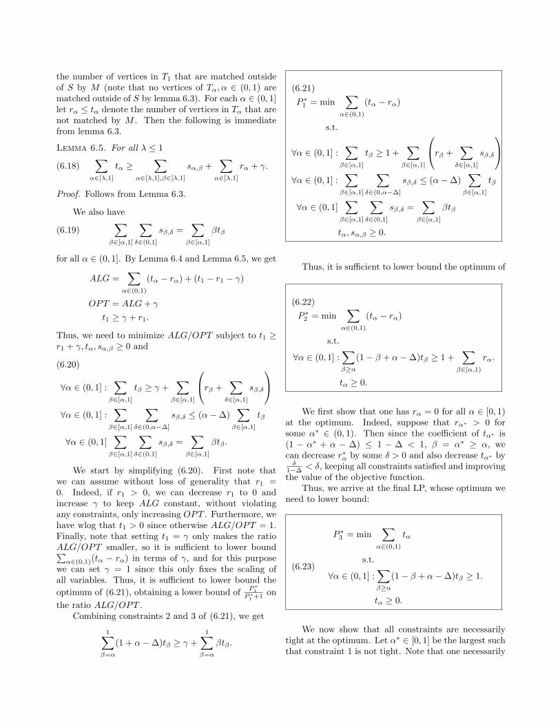
that are matched outsideof S by M (note that no vertices of T↵,↵ 2 (0, 1) arematched outside of S by lemma 6.3). For each ↵ 2 (0, 1]let r↵ t↵ denote the number of vertices in T↵ that arenot matched by M . Then the following is immediatefrom lemma 6.3.
Lemma 6.5. For all � 1
(6.18)X
↵2[�,1]
t↵ �X
↵2[�,1],�2[�,1]
s↵,� +X
↵2[�,1]
r↵ + �.
Proof. Follows from Lemma 6.3.
We also have
(6.19)X
�2[↵,1]
X
�2(0,1]
s�,� =X
�2[↵,1]
�t�
for all ↵ 2 (0, 1]. By Lemma 6.4 and Lemma 6.5, we get
ALG =X
↵2(0,1)
(t↵ � r↵) + (t1
� r1
� �)
OPT = ALG+ �
t1
� � + r1
.
Thus, we need to minimize ALG/OPT subject to t1
�r1
+ �, t↵, s↵,� � 0 and
8↵ 2 (0, 1] :X
�2[↵,1]
t� � � +X
�2[↵,1]
0
@r� +X
�2[↵,1]
s�,�
1
A
8↵ 2 (0, 1] :X
�2[↵,1]
X
�2(0,↵��]
s�,� (↵��)X
�2[↵,1]
t�
8↵ 2 (0, 1]X
�2[↵,1]
X
�2(0,1]
s�,� =X
�2[↵,1]
�t� .
(6.20)
We start by simplifying (6.20). First note thatwe can assume without loss of generality that r
1
=0. Indeed, if r
1
> 0, we can decrease r1
to 0 andincrease � to keep ALG constant, without violatingany constraints, only increasing OPT . Furthermore, wehave wlog that t
1
> 0 since otherwise ALG/OPT = 1.Finally, note that setting t
1
= � only makes the ratioALG/OPT smaller, so it is su�cient to lower boundP
↵2(0,1)(t↵ � r↵) in terms of �, and for this purposewe can set � = 1 since this only fixes the scaling ofall variables. Thus, it is su�cient to lower bound the
optimum of (6.21), obtaining a lower bound of P⇤1
P⇤1 +1
on
the ratio ALG/OPT .Combining constraints 2 and 3 of (6.21), we get
1X
�=↵
(1 + ↵��)t� � � +1X
�=↵
�t� .
P ⇤1
= minX
↵2(0,1)
(t↵ � r↵)
s.t.
8↵ 2 (0, 1] :X
�2[↵,1]
t� � 1 +X
�2[↵,1]
0
@r� +X
�2[↵,1]
s�,�
1
A
8↵ 2 (0, 1] :X
�2[↵,1]
X
�2(0,↵��]
s�,� (↵��)X
�2[↵,1]
t�
8↵ 2 (0, 1]X
�2[↵,1]
X
�2(0,1]
s�,� =X
�2[↵,1]
�t�
t↵, s↵,� � 0.
(6.21)
Thus, it is su�cient to lower bound the optimum of
P ⇤2
= minX
↵2(0,1)
(t↵ � r↵)
s.t.
8↵ 2 (0, 1] :X
��↵
(1� � + ↵��)t� � 1 +X
�2[↵,1)
r↵.
t↵ � 0.
(6.22)
We first show that one has r↵ = 0 for all ↵ 2 [0, 1)at the optimum. Indeed, suppose that r↵⇤ > 0 forsome ↵⇤ 2 (0, 1). Then since the coe�cient of t↵⇤ is(1 � ↵⇤ + ↵ � �) 1 � � < 1, � = ↵⇤ � ↵, wecan decrease r⇤↵ by some � > 0 and also decrease t↵⇤ by
�1��
< �, keeping all constraints satisfied and improvingthe value of the objective function.
Thus, we arrive at the final LP, whose optimum weneed to lower bound:
P ⇤3
= minX
↵2(0,1)
t↵
s.t.
8↵ 2 (0, 1] :X
��↵
(1� � + ↵��)t� � 1.
t↵ � 0.
(6.23)
We now show that all constraints are necessarilytight at the optimum. Let ↵⇤ 2 [0, 1] be the largest suchthat constraint 1 is not tight. Note that one necessarily
has t↵⇤ > 0. Let t0 = t� �e↵⇤ + �1+�
e↵⇤��
.We now verify that all constrains are satisfied. For
↵ > ↵⇤ all constraints are satisfied since we did notchange t. For ↵ = ↵⇤, the constraint is satisfied since itwas slack for t and � is su�ciently small.
For ↵ < ↵⇤, i.e. ↵ ↵⇤�� since we are consideringonly ↵ 2 D, we have
X
��↵
(1� � + ↵��)t0� =X
��↵
(1� � + ↵��)t�
+�
✓1� (↵⇤ ��) + ↵��
1 +�� (1� ↵⇤ + ↵��)
◆
=X
��↵
(1� � + ↵��)t� +��(↵⇤ � ↵��)
1 +�
�X
��↵
(1� � + ↵��)t� � 1.
Thus, at the optimum we have
(6.24)X
��↵
(1 + (↵� � ��))t� = 1, 8↵ 2 [0, 1].
Subtracting (6.24) for ↵+� from (6.24) for ↵, we getX
��↵
(1 + (↵� � ��))t�
�X
��↵+�
(1 + (↵+�� � ��)t�
= t↵ ��X
��↵
t� = 0.
(6.25)
In other words,
(6.26) t↵ = �X
��↵
t� , t1 � 1.
Let � = �
1��
. We now prove by induction that
t1�k� = �(1 + �)k�1 for all k > 0.
Base: k = 1 t1��
= �
1��
= �.
Inductive step: k ! k + 1
t1�(k+1)�
= �
0
@t1�(k+1)�
+ 1 + �kX
j=1
(1 + �)j�1
1
A
Thus,
t1�(k+1)�
= �
0
@1 + �kX
j=1
(1 + �)j�1
1
A
= �
✓1 + �
1� (1 + �)k
1� (1 + �)
◆= �(1 + �)k.
Hence, one has
X
↵2[0,1)
t↵ � �
1/�X
j=1
(1 + �)j�1 = �1� (1 + �)1/�
1� (1 + �)
= (1 + �)1/� � 1 =
✓1 +
�
1��
◆1/�
� 1
= (1��)�1/� � 1
Now, the size of the matching M is bounded by
OPT X
↵2[0,1)
t↵ + 1.
On the other hand,
ALG �X
↵2[0,1)
t↵.
Thus, we get
ALG
OPT=
P ⇤1
P ⇤1
+ 1= 1� 1
P ⇤1
+ 1� 1� 1
P ⇤3
+ 1
� 1� (1��)1/� � 1� 1/e
since (1��)1/� 1/e for all � � 0. We now prove
Theorem 6.1. There exists a deterministic O(n) space1-pass streaming algorithm for approximating the max-imum matching in bipartite graphs to factor 1� 1/e inthe vertex arrival model.
Proof. Run the algorithm given in (6.12), letting |Pi| =1, i.e. sparsifying as soon as a new vertex comes in. Thealgorithm only keeps a sparsifier G0
i in memory, whichtakes space O(n).
7 Constructions of Ruzsa-Szemeredi graphs
In this section we give two extensions of constructions ofRuzsa-Szemeredi graphs from [7]. The first constructionshows that for any constant ✏ > 0 there exist (1/2� ✏)-Ruzsa-Szemeredi graphs with superlinear number ofedges. We use this construction in section 8 to provethat our bound on CC(✏, n), ✏ < 1/3 is tight. Thesecond construction that we present is a generalizationto lop-sided graphs, which we use in section 8 toprove that our bound on CCv(✏, n), ✏ < 1/4 is tight.Specifically, we show the following results:
Lemma 7.1. For any constant ✏ > 0 there exists afamily of bipartite (1/2 � ✏)-Ruzsa-Szemeredi graphswith n1+⌦(1/ log logn) edges.
Lemma 7.2. For any constant � > 0 there exists a fam-ily of bipartite Ruzsa-Szemeredi graphs G = (X,Y,E)
with |X| = n, |Y | = 2n such that (1) the edge setE is a union of n⌦�(1/ log logn) induced 2-matchingsM
1
, . . . ,Mk of size at least (1/2 � O(�))|X|, and (2)for any j 2 [1 : k] the graph G contains a matching M⇤
j
of size at least (1�O(�))|X| that avoids Y \ (Mj \ Y ).
The proofs of these results are based on an adap-tation of Theorem 16 in [7] (see also [15]), which con-structs bipartite 1/3-Ruzsa-Szemeredi graphs with su-perlinear number of edges. The main idea of the con-struction, use of a large family of nearly orthogonalvectors derived from known families of error correctingcodes, is the same. A technical step is required to gofrom matchings of size 1/3 to matchings of size 1/2� ✏for any ✏ > 0. Since the result does not follow directlyfrom [7], we give a complete proof in the full version.
8 Lower bounds on communication andone-pass streaming complexity
We show here that lower bounds on the size of Ruzsa-Szemeredi graphs yield lower bounds on the (random-ized) communication complexity, and hence for one-passstreaming complexity.
In the edge model, we show that
CC⇣
2(1�✏)2�✏ � �, (2� ✏)n
⌘= ⌦(UI(✏, n)) for all
✏, � > 0. In particular, combined with the con-structions of (1/2 + �
0
)-Ruzsa-Szemeredi graphs forany constant �
0
> 0 (Lemma 7.1) this proves thatCC(✏, n) = n1+⌦(1/ log logn) for ✏ < 1/3. Thus ourO(n) upper bound on CC( 1
3
, n) in section 4 is optimalin the sense that any better approximation requiressuper-linear communication. As a corollary, we also getthat super-linear space is necessary to achieve betterthan 2/3-approximation in the one-pass streamingmodel.
In the vertex model, using the construction ofRuzsa-Szemeredi graphs from Lemma 7.2, we showthat CCv(✏, n) = n1+⌦(1/ log logn) for all ✏ < 1/4.This proves optimality of our construction in section 5,and also shows that super-linear space is necessary toachieve better than 3/4-approximation in the one-passstreaming model even in the vertex arrival setting.
We note that our lower bounds for both the edgeand vertex arrival case apply to randomized algorithms.The proofs of these results appear in the full version.
8.1 Edge arrivals
Lemma 8.1. For any ✏ > 0 and � > 0,
CC⇣
2(1�✏)2�✏ � �, (2� ✏)n
⌘= ⌦(UI(✏, n)).
Proof. For any � > 0, we will construct a distributionover bipartite graphs with (2 � ✏)n vertices on each
side such that each graph in the distribution containsa matching of size at least (2 � ✏)n � �n. On theother hand, we will define a partition of the edge setE of the graph into E = E
1
[ E2
and show that anyfor deterministic communication protocol using messagesize s = o(UI(✏, n)), the expected size of the matchingcomputed is bounded by 2(1 � ✏)n + o(n). UsingYao’s minmax principle, we get the desired performancebound for any protocol with o(UI(✏, n)) communication.
Let G = (P,Q,E) be an ✏-RS graph with n verticeson each side and UI(✏, n) edges. By definition, E can bepartitioned into k induced matchings M
1
, ...,Mk, where|Mi| = ✏n for 1 i k, and k = UI(✏, n)/(✏n). Wegenerate a random bipartite graph G0 = (P
1
[ P2
, Q1
[Q
2
, E1
[ E2
) with (2 � ✏)n vertices on each side, asfollows:
1. We set P1
= P and Q1
= Q. Also, let P2
and Q2
be a set of (1 � ✏)n vertices each that are disjointfrom P and Q.
2. For each Mi, i = 1, ..., k, let M 0i be a uniformly at
random chosen subset of Mi of size (1 � �)n. Weset E
1
= [ki=1
M 0i .
3. Choose a uniformly random r 2 [1 : k]. Let M⇤1
be an arbitrary perfect matching between P2
andQ \ Q
1
(Mr), and let M⇤2
be an arbitrary perfectmatching between Q
2
and P \ P1
(Mr). We setE
2
= M⇤1
[M⇤2
.
The instance G0 is partitioned between Aliceand Bob as follows: Alice is given all edges inG
1
(P1
, Q1
, E1
) (first phase), and Bob is given all edgesin G
2
(P2
, Q2
, E2
) (second phase). Clearly, any optimalmatching in G0 has size at least (2� ✏)n� �n; consider,for instance, the matching M 0
r [M⇤1
[M⇤2
.We now show that for any deterministic commu-
nication protocol using communication at most s =o(UI(✏, n)), with probability at least (1 � o(1)), num-ber of edges in M 0
r retained by the algorithm at the endof the first phase is o(n). Assuming this claim, we getthat with probability at least (1� o(1)), the size of thematching output by Bob is bounded by 2(1�✏)n+o(n).Hence the expected size of the matching output by Bobis bounded by 2(1 � ✏)n + o(n). We now establish thepreceding claim.
We start by observing that the number of distinctfirst phase graphs is at least (assume � < ✏/2)
✓✏n
�n
◆k
=
✓✏n
�n
◆UI (✏,n)✏n
= 2�UI(✏,n),
for some positive � bounded away from 0. Let Gdenote the set of all possible first phase graphs, and let
� : G ! {0, 1}s be the mapping used by Alice to mapgraphs in G to a message of size s = o(UI(✏, n)). Forany graph H 2 G, let �(H) = {H 0 | �(H 0) = �(H)}.Then note that for any graph H 2 G, Bob can outputan edge e in the solution i↵ e occurs in every graphH 0 2 �(H). For any subset F of G, let GF denote theunique graph obtained by intersection of all graphs inF (i.e. the graph GF contains an edge e i↵ e is presentin every graph in the family F ).
Claim 8.1. For any 0 < ✏0 < ✏2
and any subset F ofG, let I ✓ {1, 2, ..., k} be the set of indices such that GF
contains at least ✏0n edges from Mi for each i 2 I. Thenif |F | � 2(��o(1))UI(✏,n), |I| = o(k).
The details of the proof are deferred to the full versionof the paper.
To conclude the proof, we note that a simple count-ing argument shows that for a uniformly at random cho-sen graph H 2 G, with probability at least 1 � o(1),we have |�(H)| � 2(��o(1))UI(✏,n). Conditioned on thisevent, it follows from claim 8.1 that for a randomly cho-sen index r 2 [1..k], with probability at least 1 � o(1),the graph G
�(H)
contains at most ✏0n edges from Mr.
In particular, we get
Corollary 8.1. For any � > 0, CC(2/3 + �, n) =n1+⌦�(1/ log logn).
Proof. Follows by putting together Lemma 7.1 andLemma 8.1.
Lower bounds on communication complexity trans-late directly into bounds on one-pass streaming com-plexity:
Corollary 8.2. For any constant � > 0 any (possiblyrandomized) one-pass streaming algorithm that achieves
approximation factor 2(1�✏)2�✏ + � must use ⌦(UI(✏, n))
space. In particular, any one-pass streaming algorithmthat achieves approximation factor 2/3 + � must usen1+⌦�(1/ log logn) space.
Proof. Follows by Lemma 7.1 and Lemma 8.1.
8.2 Vertex arrivals We now prove a lower boundon the communication complexity in the vertex ar-rival model using the construction of lop-sided Ruzsa-Szemeredi graphs from Lemma 7.2. The bound impliesthat our upper bound from section 5 is tight. Moreover,the bound yields the first lower bound on the streamingcomplexity in the vertex arrival model.
Lemma 8.2. For any constant � > 0, CC1
v (3/4+�, n) =n1+⌦�(1/ log logn).
Proof. For su�ciently small � > 0, we will construct adistribution over bipartite graphs with (2+ �)n verticeson each side such that each graph in the distributioncontains a matching of size at least (2 � O(�))n. Onthe other hand, we will show that for any deterministicprotocol using space s = n1+o(1/ log logn), the expectedsize of the matching computed is bounded by (3/2 +O(�))n + o(n). Using Yao’s minmax principle we getthe desired performance bound for any n1+o(1/ log logn)-space randomized protocol.
Let G = (P,Q,E) be an (1/2 � �)-RS graphwith |P | = n, |Q| = 2n and n1+⌦(1/ log logn) edges,as guaranteed by Lemma 7.2. By definition, E canbe partitioned into k induced 2-matchings M
1
, ...,Mk,where |Mi| � (1/2 � �0)n for 1 i k, and k =n⌦(1/ log logn) and some �0 = O(�). We generate arandom bipartite graph G0 = (P
1
[P2
, Q,E1
[E2
) with(2 + �0)n vertices on each side, as follows:
1. We set P1
= P and let P2
be a set of (1 + �0)nvertices that are disjoint from P .
2. For each Mi, i = 1, ..., k, let M 0i be a uniformly at
random chosen subset of Mi of size (1/2 � 2�0)n.We set E
1
= [ki=1
M 0i .
3. Choose a uniformly random r 2 [1 : k]. Let M⇤
be an arbitrary perfect matching between P2
andQ \Q(Mr). We set E
2
= M⇤.
Let Alice hold the graph GA(P1
, Q1
, E1
) and letBob hold the graph G
2
= (P2
, Q,E2
). By Lemma 7.2,there exists a matching M⇤
r that matches at least a(1 � �0) fraction of X and avoids Q \ Q(Mr). Thus,any optimal matching in GA [GB has size at least (2�O(�))n; consider, for instance, the matching M⇤
r [M⇤.However, no deterministic space protocol can out-
put more than a �00 = O(�0) fraction of the edges in M 0r
if it uses n1+o�00 (1/ log logn) space by the same argumentas in 8.1. Hence, the size of the matching output by theprotocol is bounded above by (1/2+O(�))|P
1
|+ |P2
| =(3/2 +O(�))n.
We immediately get
Corollary 8.3. For any constant � > 0 any (possiblyrandomized) one-pass streaming algorithm that achievesapproximation factor 3/4+ � must use n1+⌦�(1/ log logn)
space.
9 Matching covers & Ruzsa-Szemeredi graphs
In this section we prove that the size of the smallestpossible matching cover is essentially the same as thenumber of edges in the largest Ruzsa-Szemeredi graphwith appropriate parameters.
We are now ready to state the two theorems thatuse induced matchings to bound the size of matchingcovers. The lower bound is easy, and is proved first.The upper bound is more intricate, and is presented insection 9.1.
Theorem 9.1. [Lower bound] For any � > 0,
LC(✏, n) � UI ((1 + �)✏, n) ·⇣
�1+�
⌘.
Proof. Let c = 1 + �. By definition, there exists anundirected bipartite graph G = (P,Q,E) with |E| =UI(✏c, n), |P | = |Q| = n, and an induced partition Fof G such that every set in the partition is of size atleast ✏cn. Consider the smallest ✏-matching-cover H ofG, and any set F 2 F . Recall that by the definitionof an induced matching, the edges in F are the onlyedges between P (F ) and Q(F ). Since F is a matchingbetween P (F ) and Q(F ), and the size of F is at least✏cn, the intersection of H and F must be of size at least|F |� ✏n, which is at least |F | ·
�c�1
c
�. Summing over all
sets F in the partition F , we get that |H| � |E| ·�c�1
c
�,
which proves the theorem.
In particular, choosing � = 1, we get LC(✏, n) �UI(2✏, n)/2. The upper bound is more complicated; wefirst state a simplified version (Theorem 9.2), and thenthe full version (Theorem 9.3). The simple version is acorollary of the full version; the full version is proved insection 9.1.
Theorem 9.2. [Simplified upper bound] Assume0 < ✏ < 2/3, 0 < � < 1, and ✏n � 3. Then,
LC(n, ✏) UI((1� �)✏, n) ·O⇣
log(1/✏)�(1��)
⌘.
Theorem 9.3. [Upper bound] Assume ✏n � 3, and0 < � < 1. Then,
LC(n, ✏) UI((1� �)✏, n) ·✓
8✏n
✏n� 1
◆·
·✓1 + log(1/✏) +
log(✏n)
8✏n
◆·✓
1
�(1� �)
◆.
We state the full expression in the above theorem as op-posed to using asymptotic notation since the constantsare simple, and it is conceivable that one may chooseto apply it in regimes where ✏ is arbitrarily close to 1.Choosing � = 1/2 in Theorem 9.2, we get the interestingspecial case, LC(n, ✏) = O(UI(✏/2, n) log(1/✏)).
9.1 Proof of the Upper Bound We will now proveTheorem 9.3. Assume we are given an arbitrary undi-rected bipartite graph G = (P,Q,E) with |P | = |Q| =n. Assume that ✏n is an integer. Also assume that ✏nis at least 3 (of course the most interesting case is when
✏ > 0 is some constant). Before proceeding, we needanother definition:
Definition 9.1. A pair (A,B), where A ✓ P and B ✓Q, is said to be “critical” if |A| = |B| = ME(A,B) =✏n, i.e. A,B are both of size ✏n and there is a perfectmatching between them. Let C denote the set of allcritical pairs in G.
We will now consider a primal-dual pair of LinearPrograms. By strong duality, the optimum objectivevalue for both LPs is the same; denote this value asZ⇤. We label the constraints in the primal with thecorresponding variable in the dual, and vice versa, forclarity.
PRIMAL: Z⇤ = minPe2E
xe
s.t.:8(A,B) 2 C :
Pe2E\(A⇥B)
xe � 1 [�A,B ]
x � 0
DUAL: Z⇤ = maxP
(A,B)2C�A,B
s.t.:8(e) 2 E :
P(A,B)2C:
e2E\(A⇥B)
�(A,B)
1 [xe]
� � 0
We will relate the size of an ✏-matching-cover of Gto the primal and the size of an ✏-induced partition of Gto the dual. In particular, in the next two subsections,we will prove the following two lemmas:
Lemma 9.1. The graph G has an ✏-matching-cover ofsize at most
✓✏n
✏n� 1
◆· (2✏n(1 + log(1/✏)) + log(✏n)) · Z⇤.
Lemma 9.2. There exists a graph G0 = (P,Q,E0) withE0 ✓ E such that |E0| � Z⇤�(1 � �)✏n/4 edges, and G0
has a (1��)✏-induced partition. Hence, UI(n, (1��)✏) �Z⇤�(1� �)✏n/4.
Theorem 9.3 is immediate from these two lemmas.
9.1.1 Proof of Lemma 9.1 A set of edges F ✓ Eis said to satisfy a pair (A,B) if |F \ (A⇥B)| > 0. Wewill further break down the proof of Lemma 9.1 in twoparts.
Lemma 9.3. If F satisfies all critical pairs, then F isan ✏-matching-cover.
Proof. The proof is by contradiction. Suppose F satis-fies all critical pairs, but there exists a pair (A,B) suchthat A ✓ P , B ✓ Q, and MF (A,B) < ME(A,B) � ✏n.Consider an arbitrary maximum matching in the graph(A,B,E \ (A ⇥ B)), say H. Discard all vertices fromA and B that are not incident on an edge in H,to obtain A0 ✓ A, B0 ✓ B. It is still true thatMF (A0, B0) < ME(A0, B0) � ✏n, but now we also knowthat ME(A0, B0) = |H| = |A0| = |B0|. Consider thegraph G0 = (A0, B0, F ). By Hall’s theorem, there existsa set A00 ✓ A0 and another set B00 ✓ B0 such that (a)|A00| > |B00| + ✏n, and (b) |F \ (A00 ⇥ (B0 \ B00))| = 0.Since H is perfect matching in the graph (A0, B0, E),there must exist at least ✏n edges of H that go from A00
to B0 \B00; let H 0 denote an arbitrary set of ✏n edges ofH that go from A00 to B0 \ B00. Let C denote the end-points of these edges in P and D denote the endpointsof these edges in Q. Then, |C| = |D| = ✏n and there isa perfect matching between C and D in E, i.e., the pair(C,D) is critical. But there is no edge between C andD in F (by construction), and hence F does not satisfyall critical pairs, which contradicts our assumption.
Lemma 9.4. There exists a set F of size at most
✓✏n
✏n� 1
◆· (2✏n(1 + log(1/✏)) + log(✏n)) · Z⇤
that satisfies all critical pairs.
Proof. First note that the number of critical pairs is at
most� n✏n
�2
<�en✏n
�2✏n
= e2✏n(1+log(1/✏)).We will now define a simple randomized rounding
procedure for the solution x of the primal LP. For con-venience, let � denote the quantity (2✏n(1+ log(1/✏))+log(✏n)). For each edge e, let xe denote a Bernoulli ran-dom variable which takes the value 1 with probabilitype = min{1, �xe}, and let all xe’s be independent. LetF denote the set of edges e for which xe = 1.
We will now define two bad events: Let ⇠1
denote
the event that |F | > �Z⇤⇣
✏n✏n�1
⌘. Let ⇠
2
denote the
event that F does not satisfy all critical sets.By construction, E[|F |] = E[
Pe xe] �
Pe xe =
�Z⇤. Hence, by Markov’s inequality, Pr[⇠1
] < ✏n�1
✏n =1� 1/(✏n).
Fix an arbitrary critical set (A,B). If there existsan edge e 2 E \ (A ⇥ B) such that pe = 1 then (A,B)is deterministically satisfied by F . Else, it must be thatpe = �xe for every edge e 2 E \ (A ⇥ B), and the
probability that F does not satisfy (A,B) is at most
Y
e2E\(A⇥B)
(1� �xe)
e��P
e2E\(A⇥B) xe
e�� ,
where the third line follows from the second fromfeasibility of the fractional solution. Using the unionbound over all critical pairs, we get Pr[⇠
2
] < e� log(✏n) =1/(✏n). Using the union bound over the two badevents, we get Pr[⇠
1
[ ⇠2
] < 1. Hence, (using theprobabilistic method), there must exist a set of edgesF that satisfies all critical pairs and has size at most⇣
✏n✏n�1
⌘· (2✏n(1 + log(1/✏)) + log(✏n)) · Z⇤.
This concludes the proof of Lemma 9.1.
9.1.2 Proof of Lemma 9.2 This proof is also viarandomized rounding, this time applied to the optimumsolution of the dual LP. For every relevant pair (A,B),choose �A,B to be one with probability ��A,B/2 and 0otherwise; further choose the values of di↵erent �A,B ’sindependently. If �A,B = 1 then we say that the pair(A,B) has been selected. Initialize H to be E; we willremove edges from H till the graph (P,Q,H) has an✏-induced partition.
Step 1: Getting an induced partition. First,fix an arbitrary perfect matching (in E) between eachselected pair, and (a) remove all edges from H that donot belong to any of these perfect matchings. Then, (b)remove all edges that belong to more than one of thegraphs induced by the selected pairs. Let the new setof edges be called H
1
.Step 2: Pruning small induced sets. At this
point, the collection of sets of edges {(A ⇥ B) \ H1
:�A,B = 1} forms an induced partition of the graph(P,Q,H
1
). The only problem is that some of the sets inthis partition may be too small. We will count a selectedpair (A,B) as “good” if it induces at least (1��)✏n edgesin H
1
, and “bad” otherwise. Remove all edges from H1
that are induced by a bad selected pair to obtain theset H
2
. The set (P,Q,H2
) now has a ((1� �)✏)-inducedpartition. Let k denote the number of good selectedpairs; then |H
2
| (and hence UI(n, (1 � �)✏)) is at leastk(1� �)✏n.
We will now show that Pr[k > �Z⇤/4] > 0.Consider a relevant pair (A,B) with �A,B > 0. Now,Pr[�A,B = 1] = ��A,B/2. Consider the perfectmatching F chosen between this pair (arbitrarily) instep 1 and consider any edge e in this matching. Thisedge will not be pruned away in step 1(a). By the
feasibility constraint in the dual,
X
(A0,B0)2C:(A,B) 6=(A0,B0
),e2E\(A0⇥B0)
�A0,B0 < 1.
Hence, the probability that this edge will belong to aselected pair other than (A,B) is less than �/2. Thus,the expected number of edges in H
1
\ (A⇥ B) is morethan (1 � �/2)✏n. The maximum number of edges inH
1
\ (A ⇥ B) is ✏n. Applying Markov’s inequality tothe random variable ✏n� |H
1
\ (A⇥B)|, we get:
Pr[|H1
\ (A⇥B)| � (1� �)✏n | �A,B = 1] > 1/2.
Multiplying with the probability that �A,B = 1, weobtain:
Pr[A relevant pair (A,B) is both selected and good]
> ��A,B/4.
Summing over all relevant pairs (A,B), we get E[k] >�Z⇤/4, and hence (using the probabilistic methodagain), there must exist a set of choices for �A,B whichmake k > �Z⇤/4. For this choice, we know that H
2
(and hence UI(n, (1� �)✏)) is at least Z⇤�(1� �)✏n/4.This concludes the proof of Lemma 9.2.Finally, we note that an upper bound on the
size of ✏-covers directly yields an upper bound on thecommunication complexity of achieving an additive ✏nerror approximation to bipartite matching, denoted byCC
+
(✏, n).
Lemma 9.5. CC+
(✏, n) LC(✏, n).
Proof. Let G1
= (P1
, Q1
, E1
) denote the bipartite graphwith |P | = |Q| = n that Alice holds and let G
2
=(P
2
, Q2
, E2
) be the graph that Bob holds. Let G01
be a✏-matching cover of G
1
. Consider an empty cut (A1
[B
1
, A2
[B2
) corresponding to a maximum matching M 0
in (G01
[G2
), i.e. such that |M 0| = |B1
|+ |A2
|. Let M⇤
denote a maximum matching in (A1
⇥ B2
) \ E1
. SinceG0
1
is an ✏-matching cover, we have that |M⇤| < ✏n.Thus, since the maximum matching M in G
1
[G2
is bounded by |B1
|+ |A2
|+ |M⇤| we have
|M |� |M 0| (|B1
|+ |A2
|+ |M⇤|)� (|B1
|+ |A2
|) ✏n.
References
[1] K. Ahn and S. Guha. Laminar families and metric em-beddings: Non-bipartite maximum matching problemin the semi-streaming model. CoRR, abs/1104.4058,2011.
[2] K. Ahn and S. Guha. Linear programming in the semi-streaming model with application to the maximummatching problem. ICALP, pages 526–538, 2011.
[3] F. A. Behrend. On sets of integers which contain nothree terms in arithmetic progression. Proc. Nat. Acad.Sci., 32:331–332, 1946.
[4] Andras A. Benczur and David R. Karger. Approximat-ing s-t minimum cuts in O(n2) time. Proceedings of the28th annual ACM symposium on Theory of computing,pages 47–55, 1996.
[5] Sebastian Eggert, Lasse Kliemann, and Anand Srivas-tav. Bipartite graph matchings in the semi-streamingmodel. ESA 2009, pages 492–503, 2009.
[6] Joan Feigenbaum, Sampath Kannan, Andrew McGre-gor, Siddharth Suri, and Jian Zhang. On graph prob-lems in a semi-streaming model. Theor. Comput. Sci.,348:207–216, 2005.
[7] E. Fischer, E. Lehman, I. Newman, S. Raskhodnikova,R. Rubinfeld, and A. Samorodnitsky. Monotonicitytesting over general poset domains. STOC, 2002.
[8] A. Goel, A. Meyerson, and S. Plotkin. Approximatemajorization and fair online load balancing. ACMTransactions on Algorithms, 1(2):338–349, Oct 2005.
[9] T. W. Gowers. Some unsolved problemsin additive/combinatorial number theory.http://www.dpmms.cam.ac.uk/ wtg10/addnoth.survey.dvi.
[10] J. Hastad and A. Wigderson. Simple analysis of graphtests for linearity and pcp. Random Structures andAlgorithms, 22, 2003.
[11] D. Karger. Random sampling in cut, flow, and networkdesign problems. Mathematics of Operations Research(Preliminary version appeared in the Proceedings of the26th annual ACM symposium on Theory of comput-ing), 24(2):383–413, 1999.
[12] R. Karp, U. Vazirani, and V. Vazirani. An optimalalgorithm for online bipartite matching. STOC, 1990.
[13] J. Kleinberg, Y. Rabani, and E. Tardos. Fairness inrouting and load balancing. J. Comput. Syst. Sci.,63(1):2–20, 2001.
[14] A. McGregor. Finding graph matchings in datastreams. APPROX-RANDOM, pages 170–181, 2005.
[15] S. Raskhodnikova. Property testing: Theory andapplications. Ph.D. thesis, 2003.
[16] A. Schrijver. Combinatorial Optimization. SpringerVerlag, 2003.
[17] T. Tao and V. Vu. Additive Combinatorics. CambridgeUniversity Press, 2009.