on the block maxima method in extreme value theory: pwm

The Annals of Statistics2015, Vol. 43, No. 1, 276–298DOI: 10.1214/14-AOS1280© Institute of Mathematical Statistics, 2015

ON THE BLOCK MAXIMA METHOD IN EXTREME VALUETHEORY: PWM ESTIMATORS1

BY ANA FERREIRA AND LAURENS DE HAAN

University of Lisbon and Erasmus Univ Rotterdam

In extreme value theory, there are two fundamental approaches, bothwidely used: the block maxima (BM) method and the peaks-over-threshold(POT) method. Whereas much theoretical research has gone into the POTmethod, the BM method has not been studied thoroughly. The present paperaims at providing conditions under which the BM method can be justified.We also provide a theoretical comparative study of the methods, which is ingeneral consistent with the vast literature on comparing the methods all basedon simulated data and fully parametric models. The results indicate that theBM method is a rather efficient method under usual practical conditions.

In this paper, we restrict attention to the i.i.d. case and focus on the prob-ability weighted moment (PWM) estimators of Hosking, Wallis and Wood[Technometrics (1985) 27 251–261].

1. Introduction. The block maxima (BM) approach in extreme value theory(EVT), consists of dividing the observation period into nonoverlapping periods ofequal size and restricts attention to the maximum observation in each period [see,e.g., Gumbel (1958)]. The new observations thus created follow—under domain ofattraction conditions, cf. (2) below—approximately an extreme value distribution,Gγ for some real γ . Parametric statistical methods for the extreme value distribu-tions are then applied to those observations.

In the peaks-over-threshold (POT) approach in EVT, one selects those of the ini-tial observations that exceed a certain high threshold. The probability distributionof those selected observations is approximately a generalized Pareto distributionPickands (1975).

In the case of the POT method, exact conditions under which the statisticalmethod is justified can be described by a second-order term [see, e.g., Drees (1998)and de Haan and Ferreira (2006), Section 2.3]. In the case of block maxima, usu-ally it is taken for granted that the maxima follow very well an extreme valuedistribution. In this paper, we take this misspecification into account by quantify-ing it in terms of a second-order expansion; cf. Condition 2.1 below. Since Gγ isnot the exact distribution for those observations, a bias may appear.

Received April 2014; revised August 2014.1Supported in part by FCT Project PTDC /MAT /112770 /2009; EXPL/MAT-STA/0622/2013 and

PEst-OE/MAT/UI0006/2014.MSC2010 subject classifications. Primary 62G32; secondary 62G20, 62G30.Key words and phrases. Block maxima, peaks-over-threshold, probability weighted moment esti-

mators, extreme value index, asymptotic normality, extreme quantile estimation.

276

http://www.imstat.org/aos/

http://dx.doi.org/10.1214/14-AOS1280

http://www.imstat.org

http://www.ams.org/mathscinet/msc/msc2010.html

ON THE BLOCK MAXIMA METHOD 277

The POT method picks up all “relevant” high observations. The BM method onthe one hand misses some of these high observations and, on the other hand, mightretain some lower observations. Hence the POT seems to make better use of theavailable information.

There are practical reasons for using the BM method:

• The only available information may be block maxima, for example, yearly max-ima with long historical records or long range simulated data sets Kharin et al.(2007).

• The BM method may be preferable when the observations are not exactly inde-pendent and identically distributed (i.i.d.). For example, there may be a seasonalperiodicity in case of yearly maxima or, there may be short range dependencethat plays a role within blocks but not between blocks; cf. for example, Katz,Parlange and Naveau (2002) and Madsen, Rasmussen and Rosbjerg (1997) forfurther discussion.

• The BM method may be easier to apply since the block periods appear naturallyin many situations [Naveau et al. (2009), van den Brink, Können and Opsteegh(2005), de Valk (1993)]. On the other hand, the POT method allows for greaterflexibility in many cases since it might be difficult to change the block size inpractice.

When working with BM, there are two sets of estimators that are widely used:the maximum likelihood (ML) estimators [e.g., Prescott and Walden (1980)] andthe probability weighted moment (PWM) estimators Hosking, Wallis and Wood(1985). Recently, Dombry (2013) has proved consistency of the former. Thepresent paper concentrates on the latter. Our work has given rise to the paperBücher and Segers (2014) on the multivariate case.

The PWM estimators under the Gγ model are very popular, for example, inapplications to hydrologic and climatologic extremes, because of their computa-tional simplicity, good performance for small sample sizes and robustness even forlocation and scale parameters [Diebolt et al. (2008), Katz, Parlange and Naveau(2002), Caires (2009), Hosking (1990)].

The relative merits of POT and BM have been discussed in several papers, allbased on simulated data: Cunnane (1973) states that for γ = 0 and ML estimators,the POT estimate for a high quantile is better only if the number of exceedancesis larger than 1.65 times the number of blocks; Wang (1991) writes that POT isas efficient as BM model for high quantiles, based on PWM estimators; Madsen,Pearson and Rosbjerg (1997) and Madsen, Rasmussen and Rosbjerg (1997) writethat POT is preferable for γ > 0, whereas for γ < 0, BM is more efficient, againwith the number of exceedances larger than the number of blocks; Martins andStedinger (2001) state that the gains (when using historical data) with the BMmodel are in the range of the gains with the POT model, based on ML estimators;Caires (2009) in a vast simulation study writes that with POT samples having anaverage of two or more observations per block, the estimates are more accurate

278 A. FERREIRA AND L. DE HAAN

than the corresponding BM estimates, and with more than 200 years of data theaccuracies of the two approaches are similar and rather good, based on severalestimators including the PWM and ML estimators.

From all these studies, some even with mixed views, the following two fea-tures seem dominant. First, POT is more efficient than BM in many circumstances,though needing, on average, a number of exceedances larger than the number ofblocks. Secondly, POT and BM often have comparable performances, for example,for large sample sizes.

Our theoretical comparison shows that BM is rather efficient. The asymptoticvariances of both extreme value index and quantile estimators are always lower forBM than for POT. Moreover, the approximate minimal mean square error is alsolower for BM under usual circumstances. The optimal number of exceedances isgenerally higher than the optimal number of blocks.

The paper is organized as follows. In Section 2, we state exact conditions tojustify the BM method, along with the asymptotic normality result for the PWMestimators including high quantile estimators. In Section 3, we provide a theoreti-cal comparison between the two methods, BM and POT. The analysis is based ona uniform expansion of the relevant quantile process given in Section 2.1. This ex-pansion also provides a basis for analysing alternative estimators besides the PWMestimator. Proofs are postponed to Section 4.

Throughout the paper, we assume that the observations are i.i.d. In future work,we shall extend the results to the non-i.i.d. case and to the maximum likelihoodestimator.

2. The estimators and their properties. Let X1, X2, . . . be i.i.d. randomvariables with distribution function F . Define for m = 1,2, . . . and i = 1,2, . . . , k

the block maxima

Xi = max(i−1)m<j≤im

Xj .(1)

Hence, the m×k observations are divided into k blocks of size m. Write n = m×k,the total number of observations. We study the model for large k and m, hence weshall assume that n → ∞; in order to obtain meaningful limit results, we have torequire that both m = mn → ∞ and k = kn → ∞, as n → ∞.

The main assumption is that F is in the domain of attraction of some extremevalue distribution

Gγ (x) = exp(−(1 + γ x)−1/γ )

, γ ∈R,1 + γ x > 0,

that is, for appropriately chosen am > 0 and bm and all x

limm→∞P

(Xi − bm

am

≤ x

)= lim

m→∞Fm(amx + bm)

(2)= Gγ (x), i = 1,2, . . . , k.


This can be written as

limm→∞

1

m

1

− logF(amx + bm)= (1 + γ x)1/γ ,

which is equivalent to the convergence of the inverse functions:

limm→∞

V (mx) − bm

am

= xγ − 1

γ, x > 0,

with V = (−1/ logF)←. Hence, bm can be chosen to be V (m). This is the first-order condition. For our analysis, we also need a second-order expansion as fol-lows.

CONDITION 2.1 (Second-order condition). Suppose that for some positivefunction a and some positive or negative function A with limt→∞ A(t) = 0,

limt→∞

(V (tx) − V (t))/a(t) − (xγ − 1)/γ

A(t)=

∫ x

1sγ−1

∫ s

1uρ−1 duds = Hγ,ρ(x),

for all x > 0 [see, e.g., de Haan and Ferreira (2006), Theorem B.3.1]. Note that thefunction |A| is regularly varying with index ρ ≤ 0.

Let X1,k, . . . ,Xk,k be the order statistics of the block maxima X1, . . . ,Xk . Thestatistics β0 = k−1 ∑k

i=1 Xi,k and

βr = 1

k

k∑i=1

(i − 1) · · · (i − r)

(k − 1) · · · (k − r)Xi,k, r = 1,2,3, . . . , k > r,(3)

are unbiased estimators of EX1Frm(X1) [Landwehr, Matalas and Wallis (1979)].

The PWM estimators for γ , as well as the location bm and scale am = a([m]), aresimple functionals of β0, β1 and β2. The estimator γk,m for γ is defined as thesolution of the equation

3γk,m − 1

2γk,m − 1= 3β2 − β0

2β1 − β0,

ak,m = γk,m

2γk,m − 1

2β1 − β0

�(1 − γk,m)and bk,m = β0 + ak,m

1 − �(1 − γk,m)

γk,m

,(4)

where �(x) = ∫ ∞0 tx−1e−t dt , x > 0 [Hosking, Wallis and Wood (1985)]. The ra-

tionale behind the estimator of γ becomes clear when checking the statement ofTheorem 2.3 below.


2.1. Asymptotic normality. The following theorem is the basis for analysingestimators in the BM approach. Let �u� represent the smallest integer larger thanor equal to u.

THEOREM 2.1. Assume that F is in the domain of attraction of an extremevalue distribution Gγ and that Condition 2.1 holds. Let m = mn → ∞ and k =kn → ∞ as n → ∞, in such a way that

√kA(m) → λ ∈ R. Let 0 < ε < 1/2 and

{Xi,k}ki=1 be the order statistics of the block maxima X1,X2, . . . ,Xk . Then, with{Ek}k≥1 an appropriate sequence of Brownian bridges,

√k

(X�ks�,k − bm

a0(m)− (− log s)−γ − 1

γ

)

= Ek(s)

s(− log s)1+γ+ √

kA0(m)Hγ,ρ

(1

− log s

)

+ (s−1/2−ε(1 − s)−1/2−γ−ρ−ε)oP (1),

as n → ∞, where the oP (1) term is uniform for 1/(k + 1) ≤ s ≤ k/(k + 1). Thefunctions a0(m) and A0(m) are chosen as in Lemma 4.2 below.

THEOREM 2.2. Assume the conditions of Theorem 2.1 with γ < 1/2. Then√

k

((r + 1)βr − bm

am

− Dr(γ )

)

→d (r + 1)

∫ 1

0sr−1(− log s)−1−γ E(s) ds + λIr(γ, ρ) =: Qr,

as n → ∞, jointly for r = 0,1,2,3, . . . , where →d means convergence in distri-bution, E is Brownian bridge,

Dr(ξ) = (r + 1)ξ�(1 − ξ) − 1

ξ, ξ < 1

[Dr(0) = log(r + 1) − �′(1) as defined by continuity], and

Ir(γ, ρ) =

⎧⎪⎪⎪⎪⎪⎪⎪⎪⎪⎪⎪⎪⎪⎪⎪⎪⎨⎪⎪⎪⎪⎪⎪⎪⎪⎪⎪⎪⎪⎪⎪⎪⎪⎩

1

ρ

(Dr(γ + ρ) − Dr(γ )

),

ρ �= 0,

D′r (γ ) = (r + 1)γ

γ

(−�′(1 − γ ) + log(r + 1)�(1 − γ )

− (r + 1)−γ Dr(γ )),

γ �= 0, ρ = 0,

D′r (0) = 1

2

(log2(r + 1) + �′′(1) − 2 log(r + 1)�′(1)

),

γ = 0, ρ = 0.

Note that �′(1 − γ ) = ∫ ∞0 u−γ e−u(logu)du and �′′(1) = 1.97811.


REMARK 2.1. The condition√

kA(m) → λ ∈ R means that the growth of kn,the number of blocks, is restricted with respect to the growth of mn, the size ofa block, as n → ∞. In particular this condition implies that (logk)/m → 0, asn → ∞.

THEOREM 2.3. Under the conditions of Theorem 2.2, as n → ∞,√

k(γk,m − γ ) →d 1

�(1 − γ )

(log 3

1 − 3−γ− log 2

1 − 2−γ

)−1

×{

γ

3γ − 1(Q2 − Q0) − γ

2γ − 1(Q1 − Q0)

}

=: ,

√k

(ak,m

am

− 1)

→d γ(2γ − 1

)�(1 − γ )

(Q1 − Q0)

+

{log 2

γ

( −γ

1 − 2−γ+ 1

log 2

)+ �′(1 − γ )

�(1 − γ )

}

=: ,

√kbk,m − bm

am

→d Q0 + γ�′(1 − γ ) − 1 + �(1 − γ )

γ 2 + 1 − �(1 − γ )

γ

=: �;where for γ = 0 the formulas should read as (defined by continuity):

√kγk,m →d

(log 3

2− log 2

2

)−1(1

log 3(Q2 − Q0) − 1

log 2(Q1 − Q0)

),

√k

(ak,m

am

− 1)

→d 1

log 2(Q1 − Q0) +

(log 2

2+ �′(1)

),

√kbk,m − bm

am

→d Q0 − �′′(1) + �′(1).

REMARK 2.2. A slight modification of γk,m produces the explicit estimator

γ ∗k,m = 1

log 2log

(4β3 − β0

2β1 − β0− 1

),(5)

which is the solution of (4γ ∗k,m − 1)(2γ ∗

k,m − 1)−1 = (4β3 − β0)(2β1 − β0)−1. The

conditions of Theorem 2.2 imply

√k(γ ∗k,m − γ

) →d 1

�(1 − γ )

(log 4

1 − 4−γ− log 2

1 − 2−γ

)−1

×{

γ

4γ − 1(Q3 − Q0) − γ

2γ − 1(Q1 − Q0)

}.


2.2. High quantile estimation. Our estimator for xn = F←(1 − pn) =V (1/(− log(1 − pn))), with pn small, is

xk,m = bk,m + ak,m

(mpn)−γk,m − 1

γk,m

.

THEOREM 2.4. Assume the conditions of Theorem 2.2 with ρ negative, orzero with γ negative. Moreover, assume that the probabilities pn satisfy

limn→∞mpn = 0 and lim

n→∞log(mpn)√

k= 0

[in case ρ < 0 the latter can be simplified to limn→∞(logpn)/√

k = 0]. Then√

k(xk,m − xn)

amqγ (1/(mpn))→d + (γ−)2� − γ− − λ

γ−γ− + ρ

as n → ∞, where γ− = min(0, γ ) and qγ (t) = ∫ t1 sγ−1 log s ds.

3. Theoretical comparison between BM and POT methods. In this section,we develop a theoretical comparison between the BM and POT methods, by com-paring the two PWM estimators for the two methods [Hosking and Wallis (1987)and Hosking, Wallis and Wood (1985), resp., for POT and BM].

First, we introduce the PWM-POT estimators for γ and a(n/k), where k isthe number of selected order statistics, {Xn−i,n}k−1

i=0 , from the original sampleX1, X2, . . . , Xn. The statistics

Pn = 1

k

k−1∑i=0

Xn−i,n − Xn−k,n and Qn = 1

k

k−1∑i=0

i

k(Xn−i,n − Xn−k,n)

are estimators for a(n/k)(1 − γ )−1 and a(n/k)(2(2 − γ )−1), respectively. Conse-quently, the PWM estimators are

γk,n = 1 −(

Pn

2Qn

− 1)−1

and a(n/k) = Pn

(Pn

2Qn

− 1)−1

.

The quantile estimator is

xk,n = Xn−k,n + a(n/k)(k/(npn))

γk,n − 1

γk,n

.

Asymptotic normality under conditions equivalent to the ones in Theorems 2.3and 2.4 holds [see, e.g., Cai, de Haan and Zhou (2013)], if ρ ∈ [−1,0] with acaveat for ρ = −1 [for certain cases the functions A in the corresponding second-order conditions may not be the same asymptotically resulting in different valuesof λ in the limiting distributions; cf. Drees, de Haan and Li (2003)].

For BM, k is defined as the number of blocks and, for POT, k is defined as thenumber of selected top order statistics. Hence, in both cases k means the numberof selected observations. For the theoretical comparison, we confine ourselves tothe range ρ ∈ [−1,0] and γ ∈ [−1,1/2), a usual range in many applications.


FIG. 1. Asymptotic variances of γ PWM estimators with dashed line for POT.

Extreme value index estimators.

• First, we compare asymptotic variance and bias for a common value of k:The asymptotic variances of the two γ estimators are shown in Figure 1: the

curve from BM is always below the other one, meaning lower values for theasymptotic variance for all values of γ . The asymptotic biases are compared inFigure 2, through the ratio “bias BM/bias POT”. Recall that the bias depends onboth first- and second-order parameters γ and ρ. Contrary to what is observedfor the variance, the bias of BM is always larger but for ρ = 0 they are thesame regardless the value of γ , equal to 1 [or λ if one takes into account theasymptotic contribution of

√kA(n/k) to the biases].

• Next, we compare asymptotic mean square errors for the “optimal choice” of k

(i.e., that value that makes the limiting mean square error of γ − γ minimal),which is different in the two cases:

FIG. 2. Ratio of asymptotic bias of γ PWM estimators.


An asymptotic expression of the “asymptotic minimal mean square error”(MINMSE in the sequel) is obtained in the following way. Suppose ρ < 0. Firstwe find for each estimator the optimal k in the sense of minimizing the approxi-mate asymptotic mean square error. Denote by σ 2

i = σ 2i (γ ) and B2

i = B2i (γ, ρ)

(i = 1,2; “1” refers to PWM-BM and “2” refers to PWM-POT) the asymptoticvariance and squared bias of the estimators. Under Condition 2.1, we can writeA2(t) = ∫ ∞

t s(u) du with s(·) decreasing and 2ρ −1 regularly varying. The lim-iting mean square error is, approximately,

infk

(σ 2

i

k+ A2(n/k)B2

i

)(6)

or, writing r for n/k, infr ((r/n)σ 2i + B2

i

∫ ∞r s(u) du). Setting the derivative

equal to zero and using properties of regularly varying functions one finds forthe optimal choice of r , r

(i)0 ∼ (1/s)←(n)(B2

i /σ 2i )1/(1−2ρ) and, in terms of k,

k(i)0 ∼ n

(1/s)←(n)

(σ 2

i

B2i

)1/(1−2ρ)

.

Note that the optimal k(i)0 is different but of the same order for both methods.

Next, inserting k(i)0 in (6), after some manipulation we get the following asymp-

totic expression for MINMSE,

1 − 2ρ

−2ρ

(1/s)←(n)

n

(B2

i

)1/(1−2ρ)(σ 2

i

)−2ρ/(1−2ρ).

It follows that MINMSE(BM)/MINMSE(POT) is, approximately,

(B2

1 (γ, ρ)

B22 (γ, ρ)

)1/(1−2ρ)(σ 21 (γ )

σ 22 (γ )

)−2ρ/(1−2ρ)

,

which does not depend on n, just on γ and ρ.The contour plot of “MINMSE(BM)/MINMSE(POT)” is represented in Fig-

ure 3. It can be seen that the BM has lower MINMSE for a large range of (γ, ρ)

combinations. Note that this range includes γ negative and γ positive close tozero which seem to be common values in many practical situations, for exam-ple, in hydrologic and climatologic extremes. Only for γ > 0.2 approximately,MINMSE for POT can be lower depending on ρ.

Finally, comparing the optimal sample sizes (cf. Figure 4 with contour plot ofthe ratio of the optimal values of k), one sees that POT requires systematicallylarger optimal sample size even when the approximate MINMSE is smaller forPOT than BM.


FIG. 3. Contour plot for the ratio of asymptotic minimal mean square error of γ PWM estimators.

Quantile estimators. We repeat the previous analysis for the quantile estima-tors:

• The asymptotic variances of the two estimators are compared in Figure 5: againthe curve from BM is always below the other one meaning lower values for theasymptotic variance for all values of γ . In Figures 6 and 7, the asymptotic bias

FIG. 4. Contour plot for the ratio of the optimal values of k.


FIG. 5. Asymptotic variances of quantile PWM estimators with dashed line for POT.

is represented for each case separately. Note that for γ negative, the bias for BMapproaches zero when ρ ↑ 0 whereas in the POT case it escapes to −∞.

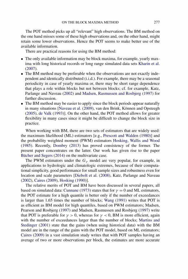
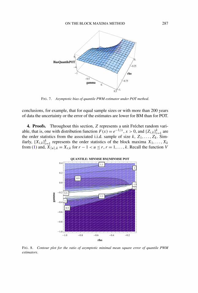
• The contour plot for the ratio “MINMSE(BM)/MINMSE(POT)” is representedin Figure 8. Again the BM method has lower MINMSE for a large range of(γ, ρ) combinations. The “irregularity” around γ ≈ −0.2 is due to a change ofsign in the bias in the POT case. Finally, Figure 9 gives the contour plot for theratio of the optimal values of k, which is smaller than one when γ is small andρ is closer to zero.

In conclusion, for both the extreme value index and quantile PWM estimators,the ones from the BM method have always lower asymptotic variances. Moreover,at an optimal level the BM gives lower MINMSE, thus being more efficient, undermany practical situations. This is in agreement with some of Sofia Caires’ (2009)

FIG. 6. Asymptotic bias of quantile PWM estimator under BM method.


FIG. 7. Asymptotic bias of quantile PWM estimator under POT method.

conclusions, for example, that for equal sample sizes or with more than 200 yearsof data the uncertainty or the error of the estimates are lower for BM than for POT.

4. Proofs. Throughout this section, Z represents a unit Fréchet random vari-able, that is, one with distribution function F(x) = e−1/x , x > 0, and {Zi,k}ki=1 arethe order statistics from the associated i.i.d. sample of size k, Z1, . . . ,Zk . Sim-ilarly, {Xi,k}ki=1 represents the order statistics of the block maxima X1, . . . ,Xk

from (1) and, X�u�,k = Xr,k for r − 1 < u ≤ r , r = 1, . . . , k. Recall the function V

FIG. 8. Contour plot for the ratio of asymptotic minimal mean square error of quantile PWMestimators.


FIG. 9. Contour plot for the ratio of the optimal values of k in quantile case.

from Section 2. The following representation will be useful:

X =d V (mZ).(7)

We start by formulating a number of auxiliary results.

LEMMA 4.1. 1. As k → ∞,

(log k)Z1,k →P 1.

2. [Csörgo and Horváth (1993), page 381] Let 0 < ν < 1/2. With {Ek}k≥1, anappropriate sequence of Brownian bridges,

sup1/(k+1)≤s≤k/(k+1)

s(− log s)

(s(1 − s))ν

∣∣∣∣√

k((− log s)Z�ks�,k − 1

) − Ek(s)

s(− log s)

∣∣∣∣ = oP (1),

as k → ∞ (�u� represents the smallest integer larger or equal to u).3. Similarly, with 0 < ν < 1/2 for an appropriate sequence {Ek}k≥1 of Brownian

bridges and ξ ∈R,

sup1/(k+1)≤s≤k/(k+1)

(s(1 − s)

)−ν

×∣∣∣∣√

ks(− log s)1+ξ

(Zξ�ks�,k − 1

ξ− (− log s)−ξ − 1

ξ

)− Ek(s)

∣∣∣∣ = oP (1),

as k → ∞.


The following is an easily obtained variant of Theorem B.3.10 of de Haan andFerreira (2006).

LEMMA 4.2. Under Condition 2.1, there are functions A0(t) ∼ A(t) anda0(t) = a(t)(1 + o(A(t))), as t → ∞, such that for all ε, δ > 0 there existst0 = t0(ε, δ) such that for t, tx > t0,

∣∣∣∣(V (tx) − V (t))/a0(t) − (xγ − 1)/γ

A0(t)− Hγ,ρ(x)

∣∣∣∣(8)

≤ ε max(xγ+ρ+δ, xγ+ρ−δ).

Moreover,∣∣∣∣a0(tx)/a0(t) − xγ

A0(t)− xγ (xρ − 1)/ρ

∣∣∣∣(9)

≤ ε max(xγ+ρ+δ, xγ+ρ−δ)

and ∣∣∣∣A0(tx)

A0(t)− xρ

∣∣∣∣ ≤ ε max(xρ+δ, xρ−δ).

Note that

Hγ,ρ(x) =

⎧⎪⎪⎪⎪⎪⎪⎪⎪⎪⎪⎪⎪⎨⎪⎪⎪⎪⎪⎪⎪⎪⎪⎪⎪⎪⎩

1

ρ

(xγ+ρ − 1

γ + ρ− xγ − 1

γ

), ρ �= 0 �= γ,

1

γ

(xγ logx − xγ − 1

γ

), ρ = 0 �= γ,

1

ρ

(xρ − 1

ρ− logx

), ρ �= 0 = γ,

1

2(logx)2, ρ = 0 = γ.

PROOF OF THEOREM 2.1. By representation (7),

X�ks�,k − bm

a0(m)− (− log s)−γ − 1

γ

=d

(V (mZ�ks�,k) − bm

a0(m)− V (m/− log s) − bm

a0(m)

)

+(

V (m/− log s) − bm

a0(m)− (− log s)−γ − 1

γ

)

= I (random part) + II (bias part).


We start with part I,

I ={(− log s)−γ V ((− log s)Z�ks�,km/− log s) − V (m/− log s)

a0(m/− log s)

}

×{a0(m/− log s)

a0(m)(− log s)γ

}

= I.1 × I.2.

According to (9) of Lemma 4.2, for each ε, δ > 0 there exists t0 such that thefactor I.2 is bounded (above and below) by

1 + A0(m)

{(− log s)−ρ − 1

ρ± ε max

((− log s)−ρ+δ, (− log s)−ρ−δ)}

provided m ≥ t0 and s ≥ e−m/t0 . According to (8) of Lemma 4.2, for factor I.1 wehave the bounds

(− log s)−γ ((− log s)Z�ks�,k)γ − 1

γ+ A0

(m

− log s

)(− log s)−γ

× {Hγ,ρ

((− log s)Z�ks�,k

) ± ε max((

(− log s)Z�ks�,k)γ+ρ+δ

,


)γ+ρ−δ)}= I.1a + I.1b

provided s ≥ e−m/t0 and m/ log k ≥ t0 [the latter inequality eventually holds truesince

√kA0(m) is bounded]. Note that m/ log k ≥ t0 implies mZ1,k ≥ 2t0 which

implies (Lemma 4.1) mZ�ks�,k ≥ 2t0 for all s.For term I.1a, we use Lemma 4.1.3:

(Z�ks�,k)γ − 1

γ− (− log s)−γ − 1

γ

is bounded (above and below) by

1√k

Ek(s)

s(− log s)1+γ± ε√

k

(s(1 − s))ν

s(− log s)1+γ,

for some ε > 0, 0 < ν < 1/2 and all s ∈ [1/(k + 1), k/(k + 1)].Next, we turn to term I.1b. By Lemma 4.2, (− log s)−γ A0(

m− log s

) is bounded(above and below) by

A0(m){(− log s)−γ−ρ ± ε max

((− log s)−γ−ρ+δ, (− log s)−γ−ρ−δ)}


provided s > e−m/t0 and m/ log k > t0. Furthermore for ρ �= 0 �= γ and s ∈ [1/(k+1), k/(k + 1)], by Lemma 4.1.3,

Hγ,ρ


)

= 1

ρ

{((− log s)Z�ks�,k)γ+ρ − 1

γ + ρ− ((− log s)Z�ks�,k)γ − 1

γ

}

= 1

ρ

{(− log s)γ+ρ

[Zγ+ρ�ks�,k − 1

γ + ρ− (− log s)−γ−ρ − 1

γ + ρ

]

− (− log s)γ[Z

γ�ks�,k − 1

γ− (− log s)−γ − 1

γ

]}

is bounded by

1

ρ

{(− log s)γ+ρ

[1√k

Ek(s)

s(− log s)1+γ+ρ± ε√

k

(s(1 − s))ν

s(− log s)1+γ+ρ

]

− (− log s)γ[

1√k

Ek(s)

s(− log s)1+γ∓ ε√

k

(s(1 − s))ν

s(− log s)1+γ

]}

= ± 2ε

ρ√

k

(s(1 − s))ν

s(− log s),

and similarly for cases other than ρ �= 0 �= γ . The remaining part of I.1b, namely±ε max(((− log s)Z�ks�,k)γ+ρ+δ, ((− log s)Z�ks�,k)γ+ρ−δ), is similar.

Part II, by the inequalities of Lemma 4.2, is bounded by

A0(m)

{Hγ,ρ

(1

− log s

)± ε max

((− log s)−γ−ρ+δ, (− log s)−γ−ρ−δ)}

hence it contributes√

kA0(m)Hγ,ρ( 1− log s

) to the result.Collecting all the terms, one finds the result. �

PROOF OF THEOREM 2.2. Let, for r = 0,1,2,3, . . . ,

J(r)k (s) = (�ks� − 1) · · · (�ks� − r)

(k − 1) · · · (k − r), s ∈ [0,1].

Note that J(r)k (s) → sr , as k → ∞, uniformly in s ∈ [0,1], and

1

k

k∑i=1

(i − 1) · · · (i − r)

(k − 1) · · · (k − r)=

∫ 1

0J

(r)k (s) ds = 1

r + 1

=∫ 1

0sr ds.


Then√

k

((r + 1)βr − bm

am

− (r + 1)γ �(1 − γ ) − 1

γ

)

= √k

((r + 1)

∫ 10 X�ks�,kJ (r)

k (s) ds − bm

am

− (r + 1)

∫ 1

0

(− log s)−γ − 1

γsr ds

)

= √k(r + 1)

∫ 1

0

(X�ks�,k − bm

am

− (− log s)−γ − 1

γ

)J

(r)k (s) ds

− √k(r + 1)

∫ 1

0

(− log s)−γ − 1

γ

(sr − J

(r)k (s)

)ds

= √k(r + 1)

∫ 1/(k+1)

0

(X�ks�,k − bm

am

− (− log s)−γ − 1

γ

)J

(r)k (s) ds

+ √k(r + 1)

∫ k/(k+1)

1/(k+1)

(X�ks�,k − bm

am

− (− log s)−γ − 1

γ

)J

(r)k (s) ds

+ √k(r + 1)

∫ 1

k/(k+1)

(X�ks�,k − bm

am

− (− log s)−γ − 1

γ

)J

(r)k (s) ds

− √k(r + 1)

∫ 1

0

(− log s)−γ − 1

γ

(sr − J

(r)k (s)

)ds

= I.1 + I.2 + I.3 + I.4.

For I.4: since (sr − J(r)k (s)) = O(1/k) uniformly in s, I.4 = O(1/

√k).

For I.1, note that ∫ 1/(k+1)

0

√kX�ks�,k − bm

am

sr ds = oP (1).(10)

This follows since, the left-hand side of (10) equals, in distribution,√k

(k + 1)r+1

V (mZ1,k) − V (m)

am

which, by Lemmas 4.1.1, 4.2 and the fact that m/ log k → ∞, is bounded (belowand above) by√

k

(k + 1)r+1

{Z

γ1,k − 1

γ+ A(m)Hγ,ρ(Z1,k) ± εA(m)max

(Z

γ+ρ+δ1,k ,Z

γ+ρ−δ1,k

)}.

This is easily seen to converge to zero in probability, since Zξ1,k/

√k =

{(log k)Z1,k}ξ log−ξ k/√

k →P 0 for all real ξ and√

kA(m) → λ. Hence, I.1 =oP (1).


Next, we show that∫ 1

k/(k+1)

√kX�ks�,k − bm

am

J(r)k (s) ds = oP (1).(11)

The left-hand side equals, in distribution, since J(r)k (s) ≡ 1 for s ∈ (k(k +1)−1,1),

(1 − k

k + 1

)√kV (mZk,k) − V (m)

am

.

Lemma 4.1 yields

V (mZk,k) − V (m)

am

= Zγk,k − 1

γ+ A(m)

{Hγ,ρ(Zk,k) ± εZ

γ+ρ+δk,k

},

which is (since Zγk,k/kγ converges to a positive random variable) of the order

OP (kγ ). Hence, the integral is of order (k + 1)−1√

kkγ which tends to zero sinceγ < 1/2.

Finally, I.2 has the same asymptotic behaviour as

(r + 1)

∫ k/(k+1)

1/(k+1)

√k

(X�ks�,k − bm

am

− (− log s)−γ − 1

γ

)sr ds,

which, by Theorem 2.1 tends to

(r + 1)

∫ 1

0sr−1(− log s)−1−γ E(s) ds + λ(r + 1)

∫ 1

0Hγ,ρ

(1

− log s

)sr ds.

For the evaluation of the latter integral note that for ξ < 1,

(r + 1)

∫ 1

0sr(− log s)−ξ ds = (r + 1)ξ−1

∫ ∞0

v−ξ e−v dv = (r + 1)ξ−1�(1 − ξ).

Moreover, note that

(r + 1)

∫ 1

0sr (− log s)−ξ − 1

ξds = (r + 1)ξ�(1 − ξ) − 1

ξ, ξ < 1

[Dr(0) = log(r + 1) − �′(1) as defined by continuity], and (r + 1) ×∫ 10 Hγ,ρ( 1

− log s)sr ds = Ir(γ, ρ). �

PROOF OF THEOREM 2.3. From Theorem 2.2, we obtain

√k

(2β1 − β0

am

− 2γ − 1

γ�(1 − γ )

)→d Q1 − Q0,

√k

(3β2 − β0

am

− 3γ − 1

γ�(1 − γ )

)→d Q2 − Q0


hence, by Cramér’s delta method,

√k

(3γk,m − 1

2γk,m − 1− 3γ − 1

2γ − 1

)

= √k

(3β2 − β0

2β1 − β0− 3γ − 1

2γ − 1

)

→d 1

�(1 − γ )

3γ − 1

2γ − 1

(γ

3γ − 1(Q2 − Q0) − γ

2γ − 1(Q1 − Q0)

).

It follows that γk,m →P γ , and hence

√k

(rγk,m − 1

rγ − 1− 1

)= √

krγk,m−γ − 1

1 − r−γ

has the same limit distribution as√

k(γk,m − γ )log r

1 − r−γ, r = 2,3.

It follows that√

k

(3γk,m − 1

2γk,m − 1− 3γ − 1

2γ − 1

)

= 3γ − 1

2γ − 1

[√k

(3γk,m − 1

3γ − 1− 1

)− √

k

(2γk,m − 1

2γ − 1− 1

)]

has the same limit distribution as3γ − 1

2γ − 1

√k(γk,m − γ )

(log 3

1 − 3−γ− log 2

1 − 2−γ

)

and, consequently,√k(γk,m − γ )

→d 1

�(1 − γ )

(log 3

1 − 3−γ− log 2

1 − 2−γ

)−1

×(

γ

3γ − 1(Q2 − Q0) − γ

2γ − 1(Q1 − Q0)

).

For the asymptotic distribution of ak,m we write

√k

(ak,m

am

− 1)

γk,m

(2γk,m − 1)�(1 − γk,m)

×{√

k

(2β1 − β0

am

− 2γ − 1

γ�(1 − γ )

)

+ √k

(2γ − 1

γ�(1 − γ ) − 2γk,m − 1

γk,m

�(1 − γk,m)

)},


and the statement follows, for example, by Cramér’s delta method.For the asymptotic distribution of bk,m, we write

√k

(bk,m − bm

am

)

= √k

(β0 − bm

am

− �(1 − γ ) − 1

γ

)

− ak,m

am

√k

(�(1 − γk,m) − 1

γk,m

− �(1 − γ ) − 1

γ

)

+ �(1 − γ ) − 1

γ

√k

(ak,m

am

− 1)

and the statement follows, for example, by Cramér’s delta method. �

PROOF OF THEOREM 2.4. The proof follows the line of the comparable resultfor the POT method [see, e.g., de Haan and Ferreira (2006), Chapter 4.3]. Letcn = 1/(mpn). Then

√k(xk,m − xn)

amqγ (cn)

=√

k

amqγ (cn)

(bk,m + ak,m

cγk,mn − 1

γk,m

− V

(1

− log(1 − pn)

))

=√

k

qγ (cn)

bk,m − bm

am

+ ak,m

am

√k

qγ (cn)

(cγk,mn − 1

γ− c

γn − 1

γ

)

−√

k

qγ (cn)

(V (m/(−m log(1 − pn))) − V (m)

am

− cγn − 1

γ

)

+ cγn − 1

γ qγ (cn)

√k

(ak,m

am

− 1).

Similarly, as on pages 135–137 of de Haan and Ferreira (2006), this converges indistribution to

+ (γ−)2� − γ− − λγ−

γ− + ρ. �

APPENDIX: ASYMPTOTIC VARIANCES AND BIASES OF THE PWMESTIMATORS

The following provides a basis for an algorithm to calculate the asymptoticvariances/covariances and biases of the PWM estimators.


Let Qr = (r + 1)∫ 1

0 sr−1(− log s)−1−γ E(s) ds + λIr(γ, ρ), r = 0,1,2, as de-fined in Theorem 2.2. For r,m = 0,1,2,

Cov(Qr,Qm)

= (r + 1)(m + 1)

×∫ 1

0

∫ 1

0sr−1um−1(− log s)−1−γ (− logu)−1−γ EB(s)B(u)ds du

(12)

= (r + 1)(m + 1)

∫ 1

0um−1(1 − u)(− logu)−1−γ

∫ u

0sr(− log s)−1−γ ds du

+ (r + 1)(m + 1)

×∫ 1

0sr−1(1 − s)(− log s)−1−γ

∫ s

0um(− logu)−1−γ duds

using the fact that EB(s)B(u) = min(s, u) − su = s(1 − u) for 0 < s < u. Theseintegrals can be evaluated numerically (we have used Mathematica software).

From Theorems 2.3 and 2.4, after some calculations,√

k(γk,m − γ ) →d Cγ (kγ,0Q0 + kγ,1Q1 + kγ,2Q2),(13)

√k

(ak,m

am

− 1)

→d ka,0Q0 + ka,1Q1 + ka,2Q2,(14)

√kbk,m − bm

am

→d kb,0Q0 + kb,1Q1 + kb,2Q2,(15)

√k(xk,m − xn)

amqγ (cn)→d kx,0Q0 + kx,1Q1 + kx,2Q2,(16)

where, for γ �= 0,

Cγ = 1

�(1 − γ )

(log 3

1 − 3−γ− log 2

1 − 2−γ

)−1

,

kγ,0 = γ (3γ − 2γ )

(3γ − 1)(2γ − 1), kγ,1 = −γ

2γ − 1, kγ,2 = γ

3γ − 1;

Ca = log 2

γ

(1

log 2− γ

1 − 2−γ

)+ �′(1 − γ )

�(1 − γ ),

ka,0 = Cγ kγ,0Ca − γ

(2γ − 1)�(1 − γ ),

ka,1 = Cγ kγ,1Ca + γ

(2γ − 1)�(1 − γ ),

ka,2 = Cγ kγ,2Ca − γ

(2γ − 1)�(1 − γ );


Cb = γ�′(1 − γ ) − 1 + �(1 − γ )

γ 2 ,

kb,0 = 1 + Cγ kγ,0Cb + kγ,01 − �(1 − γ )

γ,

kb,1 = Cγ kγ,1Cb + kγ,11 − �(1 − γ )

γ,

kb,2 = Cγ kγ,2Cb + kγ,21 − �(1 − γ )

γ;

kx,0 = Cγ kγ,0 + (γ−)2kb,0 − γ−ka,0,

kx,1 = Cγ kγ,1 + (γ−)2kb,1 − γ−ka,1, kx,2 = Cγ kγ,2 + (γ−)2kb,2 − γ−ka,2

and, for γ = 0,

Cγ = 2(log(3/2)

)−1, kγ,0 = (log 2)−1 − (log 3)−1,

kγ,1 = −(log 2)−1, kγ,2 = (log 3)−1;Ca = 2−1 log 2 + �′(1), Cb = −�′′(1)

and the rest follow similarly by continuity. Then the asymptotic variances, covari-ances and biases follow by combining (12) with (13)–(16) in the obvious way.

Acknowledgements. We thank Holger Drees for a useful suggestion.We would like to thank three unknown referees for their genuine interest and

their insightful comments.

REFERENCES

BÜCHER, A. and SEGERS, J. (2014). Extreme value copula estimation based on block maxima of amultivariate stationary time series. Extremes 17 495–528. MR3252823

CAI, J.-J., DE HAAN, L. and ZHOU, C. (2013). Bias correction in extreme value statistics withindex around zero. Extremes 16 173–201. MR3057195

CAIRES, S. (2009). A comparative simulation study of the annual maxima and the peaks-over-threshold methods. SBW-Belastingen: Subproject “Statistics”. Deltares Report 1200264-002.

CSÖRGO, M. and HORVÁTH, L. (1993). Weighted Approximations in Probability and Statistics.Wiley, Chichester. MR1215046

CUNNANE, C. (1973). A particular comparison of annual maxima and partial duration series meth-ods of flood frequency prediction. J. Hydrol. 18 257–271.

DE HAAN, L. and FERREIRA, A. (2006). Extreme Value Theory: An Introduction. Springer, NewYork. MR2234156

DE VALK, C. (1993). Estimation of marginals from measurements and hindcast data. WL|Delft Hy-draulics Report H1700.

DIEBOLT, J., GUILLOU, A., NAVEAU, P. and RIBEREAU, P. (2008). Improving probability-weighted moment methods for the generalized extreme value distribution. REVSTAT 6 35–50.MR2386298

DOMBRY, C. (2013). Maximum likelihood estimators for the extreme value index based on the blockmaxima method. Available at arXiv:1301.5611.

http://www.ams.org/mathscinet-getitem?mr=3252823





http://arxiv.org/abs/arXiv:1301.5611


DREES, H. (1998). On smooth statistical tail functionals. Scand. J. Stat. 25 187–210. MR1614276DREES, H., DE HAAN, L. and LI, D. (2003). On large deviation for extremes. Statist. Probab. Lett.

64 51–62. MR1995809GUMBEL, E. J. (1958). Statistics of Extremes. Columbia Univ. Press, New York. MR0096342HOSKING, J. R. M. (1990). L-moments: Analysis and estimation of distributions using linear com-

binations of order statistics. J. R. Stat. Soc. Ser. B Stat. Methodol. 52 105–124. MR1049304HOSKING, J. R. M. and WALLIS, J. R. (1987). Parameter and quantile estimation for the generalized

Pareto distribution. Technometrics 29 339–349. MR0906643HOSKING, J. R. M., WALLIS, J. R. and WOOD, E. F. (1985). Estimation of the generalized extreme-

value distribution by the method of probability-weighted moments. Technometrics 27 251–261.MR0797563

KATZ, R. W. PARLANGE, M. B. and NAVEAU, P. (2002). Statistics of extremes in hydrology.Advances in Water Resources 25 1287–1304.

KHARIN, V. V., ZWIERS, F. W., ZHANG, X. and HEGERL, G. C. (2007). Changes in temperatureand precipitation extremes in the IPCC ensemble of global coupled model simulations. Journalof Climate 20 1419–1444.

LANDWEHR, J., MATALAS, N. and WALLIS, J. (1979). Probability weighted moments comparedwith some traditional techniques in estimating Gumbel parameters and quantiles. Water ResourcesResearch 15 1055–1064.

MADSEN, H., PEARSON, C. P. and ROSBJERG, D. (1997). Comparison of annual maximum seriesand partial duration series methods for modeling extreme hydrologic events 2. Regional modeling.Water Resources Research 33 759–769.

MADSEN, H., RASMUSSEN, P. F. and ROSBJERG, D. (1997). Comparison of annual maximum se-ries and partial duration series methods for modeling extreme hydrologic events 1. At-site mod-eling. Water Resources Research 33 747–757.

MARTINS, E. S. and STEDINGER, J. R. (2001). Historical information in a generalized maximumlikelihood framework with partial duration and annual maximum series. Water Resources Re-search 37 2559–2567.

NAVEAU, P., GUILLOU, A., COOLEY, D. and DIEBOLT, J. (2009). Modelling pairwise dependenceof maxima in space. Biometrika 96 1–17. MR2482131

PICKANDS, J. III (1975). Statistical inference using extreme order statistics. Ann. Statist. 3 119–131.MR0423667

PRESCOTT, P. and WALDEN, A. T. (1980). Maximum likelihood estimation of the parameters of thegeneralized extreme-value distribution. Biometrika 67 723–724. MR0601119

VAN DEN BRINK, H. W., KÖNNEN, G. P. and OPSTEEGH, J. D. (2005). Uncertainties in extremesurge level estimates from observational records. Philos. Trans. R. Soc. Lond. Ser. A Math. Phys.Eng. Sci. 363 1377–1386.

WANG, Q. J. (1991). The POT model described by the generalized Pareto distribution with Poissonarrival rate. Journal of Hidrology 129 263–280.

ISADEPARTMENT OF ECONOMICS

UNIVERSITY OF LISBON

TAPADA DA AJUDA 1349-017 LISBOA

PORTUGAL

AND

CEAULFCULBLOCO C6 - PISO 4 CAMPO GRANDE

749-016 LISBOA

PORTUGAL

E-MAIL: [email protected]

DEPARTMENT OF MATHEMATICS

ERASMUS UNIVERSITY ROTTERDAM

P.O. BOX 17383000 DR ROTTERDAM

THE NETHERLANDS

AND

CEAULFCULBLOCO C6 - PISO 4 CAMPO GRANDE

749-016 LISBOA

PORTUGAL

E-MAIL: [email protected]










mailto:[email protected]

mailto:[email protected]

on the block maxima method in extreme value theory: pwm

Documents