on statistical information of extreme order … 1991 subject classifications: primary 62b10, 62g30,...

JOURNAL OF MULTIVARIATE ANALYSIS ,~, 1--30 (1994)

On Statistical Information of Extreme Order Statistics, Local Extreme Value Alternatives,

and Poisson Point Processes

A. JANSSEN

Heinrich-Heine-Universit6t D~sseldorf, D~sseldorf, Germany

AND

F. M A R O H N

Katholische Universit6t Eichsti~tt, Eichstiitt, Germany

The aim of the present paper is to clarify the r61e of extreme order statistics in general statistical models. This is done within the general setup of statistical experiments in LeCam's sense. Under the assumption of monotone likelihood ratios, we prove that a sequence of experiments is asymptotically Gaussian if, and only if, a fixed number of extremes asymptotically does not contain any information. In other words: A fixed number of extremes asymptotically contains information iff the Poisson part of the limit experiment is non-trivial. Suggested by this result, we propose a new extreme value model given by local alternatives. The local structure is described by introducing the space of extreme value tangents. It turns out that under local alternatives a new class of extreme value distributions appears as limit distributions. Moreover, explicit representations of the Poisson limit experiments via Poisson point processes are found. As a concrete example nonparametric tests for Fr6chet type distributions against stochastically larger alternatives are treated. We find asymptotically optimal tests within certain threshold models. © 1994 Academic Press, Inc.

l . INTRODUCTION AND NOTATION

The present paper aims to clarify the r61e of extreme observations within i.i.d, models of real valued random variables in the asymptotic setting. The starting points of our investigation are the recent monographs of Reiss

Received August 28, 1990; revised March 18, 1993.

MSC 1991 subject classifications: primary 62B10, 62G30, secondary 60G55. Key words and phrases: Extreme order statistics, statistical information, Gaussian

experiments, Poisson experiments, Poisson point processes, local extreme value alternatives, extreme value tangents, Fr6chet distribution, intensity model, hazard rate model.

1 0047-259X/94 $6.00

Copyright /("! 1994 by Academic Press, Inc. All rights of reproduction in any form reserved.

2 JANSSEN AND MAROHN

1,19] and Resnick 1-21] about extreme value theory where the high mathematical standard of extreme value theory is documented. On the other hand, the asymptotic statistical theory was recently deeply influenced by the description of models given by tangent cones; see Pfanzagl and Wefelmeyer [18], which goes back to earlier work of Koshevnik and Levit [ 11 ].

The investigation of the structure of extremes and their statistical experiments has two aspects, which may be described as follows:

I. What is the asymptotic contribution of a finite number of extremes for a given arbitrary model?

II. Which kind of asymptotic models can be used for extreme value problems?

The present questions can naturally be embedded in the universal applicable theory of statistical experiments of LeCam 1-12]. Recall that the asymptotic statistical properties of a given sequence of rowwise i.i.d, observations are completely described by the class of infinitely divisible limit experiments F = G ® P which can uniquely be decomposed into the product of a Gaussian experiment G and a Poisson experiment P; see LeCam [12, Chapt. 9] and Miibrodt and Strasser 1-17]. Within this concept, the relevance of a given portion of extreme order statistics is discussed in terms of their limit experiments.

The most popular models (such as those given by tangent cones) are asymptotically Gaussian models. In that case, a finite number of extremes can asymptotically be neglected without any loss of information. In these circumstances, the extremes are often suspected to be outliers and they may be thrown out for the sake of robustness. In Section 2, the main result, Theorem 2.2, shows that this is the only case where extremes may be cancelled. The Gaussian limit experiments are completely characterized by extremes: Under monotone likelihood ratios the limit experiment is Gaussian if, and only if, the extreme observations yield no information. The consequences of that result are twofold: Note first that extreme value problems cannot be described by asymptotically Gaussian experiments (including tangent cones) but Poisson experiments appear naturally. Second, the result gives a further foundation of extreme value theory which is always relevant except for the purely Gaussian limit case. The charac- terization of Gaussian limit experiments may be compared with the behaviour of central order statistics; see Example 2.3. They are, of course, non-negligible and are frequently used as rough estimators of the underlying parameter. Finally, we remark that there is a formal accordance between the present results for statistical experiments and sums of independent random variables considered earlier by Gnedenko and Koimogorov

STATISTICAL INFORMATION OF EXTREMES 3

[3] and Lo6ve [ 15]. They showed that the underlying sums are asymptotically normal if, and only if, the lower and upper extremes converge to zero in probability.

In Section 3, we show that certain Poisson limit experiments can completely be described by extremes. Note that from abstract results it is known that they can be realized by Poisson point processes; compare with the general program of LeCam [12] and Milbrodt [16]. Here, we find an explicit representation via extreme value processes of that result. The results of Section 2 suggest extreme value models given by a set of intensities of Poisson point processes, which stand for a collection of local extreme value alternatives. The local structure of alternatives is described by the space of extreme value tangents, which is introduced (Definition 3.1 ). In Section 4, a first statistical application of the concept of extreme value tangents is given by an example. We study tests for Fr6chet type distributions against stochastically larger alternatives. They have a natural interpretation within the concept of intensity measures and hazard rates. As an application, their asymptotic optimality is discussed. In order not to disturb the main ideas of the present paper, all proofs are postponed to Section 5.

For the remainder of this section, the notation is introduced and some facts concerning statistical experiments are recalled. The reader is referred to LeCam [12], LeCam and Yang [13], Milbrodt and Strasser [17], Strasser [23], and Torgersen [25].

Let E=(I2 , aa/, { P , : t e T } ) be a statistical experiment (sometimes briefly denoted by {P, : t e T}) Then E" denotes the n th product experiment of E consisting of the product measures P','. The restriction of E to some subset O c T is denoted by El o. Let

-' : aP, ( aP, ) ,p. dp. ( i dP, d(P,+ P,) \d(P~+ P,)] (o,~) {o} \d(P:+ P,)

denote the likelihood ratio of P, w.r.t. P,. Two statistical experiments E = ( 1 2 ~ , . ~ , {P, : r e T}) and F = (122, ~¢z,

{ Q , : t e T } ) are called equivalent (E~F) if the distributions of all likelihood processes of E and F coincide:

&# \ \dP ,J ,~r P" = £# \ \ d a , / , ~ r Q" ' seT.

The weak convergence of classes of experiments (w.r.t. ~ ) is defined by the weak convergence of all finite dimensional marginal distributions of the log-likelihood process. The weak convergence of E, to E is denoted by E,--* E.


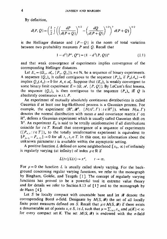
By definition,

),,2 o))"'

is the Hellinger distance and IIP-QII is the norm of total variation between two probability measures P and Q. Recall that

1 - d 2 ( P ", Q")= ( 1 - d z ( P , Q))" (1.1)

and that weak convergence of experiments implies convergence of the corresponding Hellinger distances.

Let E,, = (12,,, st,,,, {P,,, Q,,} ), n e ~, be a sequence of binary experiments. A sequence (Q,,),, is called contiguous to the sequence (P,,),, if P , , ( A , ) ~ 0 implies Q,,(A,,) ~ 0 for A,, e ~g,,. Suppose that (E,,),, is weakly convergent to some binary limit experiment E = (12, ~/, {P, Q }). By LeCam's first lemma, the sequence (Q,,),, is then contiguous to the sequence (P,,), iff Q is absolutely continuous w.r.t.P.

An experiment of mutually absolutely continuous distributions is called Gaussian if at least one log-likelihood process is a Gaussian process. For example, the experiment (R k, ~k, {N(tF, F):t~l/~k}), where N(a, 1") denotes the normal distribution with mean a and covariance matrix F on I~ k, defines a Gaussian experiment which is usually called Gaussian shift on R k. An experiment E o is said to be totally uninformative if all distributions coincide for t e T. Recall that convergence of a sequence of experiments ({P .... : t ~ T}),, to the totally uninformative experiment is equivalent to lIP,,.,,-P,,.,,II ~ 0 for all it, t2~ T. In this case, no information about the unknown parameter t is available within the asymptotic setting.

A positive function L defined on some neighborhood Ix0, ~ ) of infinitely is regularly varying (at infinity) of index p ~ R if

L(tx)/L(t) ~ x p, t ~ ~ .

For p = 0 the function L is usually called slowly varying. For the back- ground concerning regular varying functions, we refer to the monograph by Bingham, Goldie, and Teugels [1]. The concept of regularly varying functions has proved to be a powerful tool in extreme value theory and for details we refer to Section 8.13 of [1 ] and to the monograph by de Haan [4].

Let S be locally compact with countable base and let ~ denote the corresponding Borel a-field. Designate by M(S, ~ ) the set of all locally finite point measures defined on S. Recall that /~ e M(S, ~ ) if there exists a denumerable set of points xj~ S, i~ / , such that/~ = ~ ,~ i ex, and/~(K) < for every compact set K. The set M(S, ~ ) is endowed with the a-field


J[(S, ~) , which is by definition the smallest a-fled such that the projections g--* g(B), B e ~ , are measurable. The space M(S, ~) is Polish in the vague topology. Moreover, the a-field Jt '(S, ~ ) coincides with the Borel ( - B a i r e ) a-field w.r.t, the vague topology; see Kallenberg [9]). Some- times, we simply write M(S) and ./¢'(S) instead of M(S, ~) and ,//(S, ~) , respectively. A point process on (S, ~ ) is a measurable mapping N on some measurable space (I2, ~¢) into M(S, ~). An excellent introduction to the theory of point processes is the recent monograph by Reiss [20].

2. EXTREMES OF ASYMPTOTICALLY GAUSSIAN MODELS

In this section, let P,. ~ always denote continuous distributions of R, and let X~:,, ~< X2:,<~ ... <~X,:, denote the order statistics of the canonical projections X~: R " ~ R on the ith coordinate. The consideration below deals with the k-dimensional lower and upper extremes given by

W,,.k=(XI ........ Xk:,,) and Z , . k = ( X , , + l _ k ........ X .... ). (2.1)

The associated statistical experiments are abbreviated by

Ej:,,.j_<, = (R*, ~*, {Le(W,,., I e: . ,O : OE 0,,})

and E,+~_j:,,.j<~k, respectively, with W,.k replaced by Z,.k, where O , c R denotes a suitable parameter set with lo,-- , lo for some parameter set O. Throughout, we assume that 0 E O. The following two theorems show that under standard regularity assumptions asymptotic Gaussian models are not appropriate for extreme value problems. On the other hand, Theorem 2.2 is essential for extreme value theory. Note that whenever the limit experiment is not Gaussian then the extremes yield a non-negligible asymptotic contribution.

Asymptotic normality is often derived under the standard assumption of Lq-differentiability (at 0) of a given family (P,9)~ for some 1 ~< q ~< 2, which is satisfied if there exists some g e Lq(Po), called the q-derivative of the likelihood ratio, with

in Lq(Po) as ~9 ~ 0 and

,)/o . .

as oq ~ 0. By Lq(Po) we denote the space of Lq-integrable functions w.r.t. P0.

Pa \ [d (Po+Pa) - 1 =o(1~1 ~)

6 J A N S S E N A N D M A R O H N

Recall that a family (P,9).9 is called stochastically increasing if P%((x, oo))~>P~,((x, oo)) for all x e R and each pair 9~ > 3 2 . Before we state our results, note that the totally uninformative experiment Eo contains no information about the unknown parameter 3.

2.1. THEOREM. Assume that the sequence o f experiments ( R " , ~ n, { P',',. ~ :3 s O,, }) is weakly convergent to some Gaussian limit experiment G. Either let

(a) P,,.:~=P,,_~.,~ arise fi'om an Lq-differentiable family (P9),9 (at zero) for 1 <-N q <<. 2, or let

(b) (P,,.o),9 be stochastically increasing for each n.

Then for each k >1 1 the extreme value experiments Ej:, . j ~ k and E , + l - j : , , j <. k are weakly convergent to the totally uninformative experiment Eo.

Under slightly stronger conditions also the converse of Theorem 2.1 can be obtained. In that case, Gaussian limit experiments are completely characterized by the extremes. Recall that a family (P,~),~ on R has monotone likelihood ratio in x, if for each pair 9, < 9 2

dP,~ 2 dP~, (x) = h%. ~2(x) (2.2)

holds P~,+Poz-almost everywhere for some nondecreasing function h,%.,9,:R~[0, oo]. It is well known that (2.2) implies that (P9),9 is stochastically increasing; cf. Witting [26, p. 214]. The boundedness assumption of (2.3) below is standard in asymptotic theory; cf. [17, p. 40].

2.2. THEOREM. Assume that (P,,. ~ ) ~ o, admits monotone likelihood ratios in x for each n ~ N. Let the n-fold product experiment E ~ = (R ~, ~" , { P;',. ,~ : 9 e 0,, } ) be bounded, that is,

l imsupndZ(P, , . ,%,P, , .o : )<oo fo ra l131 ,32 . (2.3) n ~ 7~

Let E" be weakly convergent to some limit experiment E. For f i xed k ~ N the following assertions (a)-(c) are equivalent:

(a) E is Gaussian.

(b) For each 3 ~ 0

log dP,, ~ (Xi:,,)) i E { I . . . . . k , n + 1 - k , ..., n}

in P ,",. o" and P ,",, e-probability.

(c)

--*0

Ej:,.j<.k--* E o and En+,_j:n.j<~k---~ Eo weakly as n--* oo.


In the case of central order statistics the situation is completely different. The experiments of central order statistics are in general not negligible and often again asymptotically Gaussian, as can be seen from the next example.

2.3. EXAMPLE. Let Fdenote a distribution function on I~ with absolutely continuous Lebesgue density f and finite Fisher information !r = S (f'(x))2/ f(x) dx < ~ . Consider the stochastically increasing location family P~ with distribution functions F ( . - 9 ) .

Whenever f (F- ' (q))>O, 0 < q < l , the experiment of central order statistics

(R, ~ , {~ (xc , ,~ 1 :,, I P',',-, -',0 : 9 ~ R})

converges weakly to the one-dimensional Gaussian shift (R, M, {N(ga 2, a-'): 9e R}) with the variance

a2=f2(F l(q))(q(1-q))-~

The proof follows from Theorem 4.1.4 of Reiss [-19], where the convergence of

n'/2f(F - t(q) )(X•,,q I :,,- F- '(q))

to N(9f(F- l (q)) ,q(1-q)) under P',',-,~2:~ is proved w.r.t, the variational distance.

Finally, we discuss the median Xt,,/,_l :,, (q = ½) for 0-symmetric densities f. Its Fisher efficiency is given by 1 >t p := a'-/!r= 4f2(O)/lf. The inequality 4f2(O)<~Is is well known and can be proved directly by the Cauchy- Schwarz inequality. The discussion of the equality sign proves that the median is asymptotically efficient (w.r.t. the Fisher efficiency), that is, p = 1, if and only i f f ( x ) = e x p ( - Ixl )/2 is the density of the double exponential distribution.

3. EXTREME VALUE ALTERNATIVES AND POISSON POINT PROCESSES

As a conclusion of Section 2, we now study the precise influence of the (upper) extremes when the limit experiment is not Gaussian or only a portion of upper extremes is observable. It turns out that in various cases we find an explicit representation of the corresponding limit experiment by Poisson point processes. Let us first summarize some frequently applied approaches in extreme value theory.

Practical problems are often concerned with the upper tails of the underlying distributions. Here, we may think about the insurance mathematics,


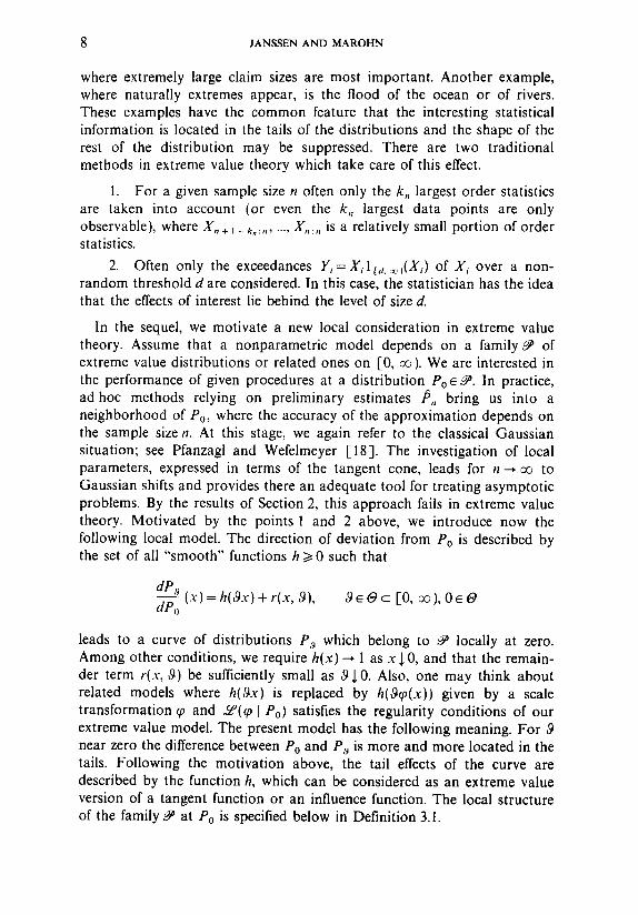
where extremely large claim sizes are most important. Another example, where naturally extremes appear, is the flood of the ocean or of rivers. These examples have the common feature that the interesting statistical information is located in the tails of the distributions and the shape of the rest of the distribution may be suppressed. There are two traditional methods in extreme value theory which take care of this effect.

1. For a given sample size n often only the k,, largest order statistics are taken into account (or even the k,, largest data points are only observable), where X,,+ ~_. ~ ......... X, .... is a relatively small portion of order statistics.

2. Often only the exceedances Yi=X~l~a.o~(Xi) of Xi over a non- random threshold d are considered. In this case, the statistician has the idea that the effects of interest lie behind the level of size d.

In the sequel, we motivate a new local consideration in extreme value theory. Assume that a nonparametric model depends on a f a m i l y ~ of extreme value distributions or related ones on [0, oe). We are interested in the performance of given procedures at a distribution Po E ~'. In practice, ad hoc methods relying on preliminary estimates /~,, bring us into a neighborhood of Po, where the accuracy of the approximation depends on the sample size n. At this stage, we again refer to the classical Gaussian situation; see Pfanzagl and Wefelmeyer [18]. The investigation of local parameters, expressed in terms of the tangent cone, leads for n--* oe to Gaussian shifts and provides there an adequate tool for treating asymptotic problems. By the results of Section 2, this approach fails in extreme value theory. Motivated by the points 1 and 2 above, we introduce now the following local model. The direction of deviation from Po is described by the set of all "smooth" functions h >~ 0 such that

dP~ (x)=h(~gx)+r(x, ~9), ~9~0c [0, ~ ) , 0 ~ O dPo

leads to a curve of distributions P.~ which belong to ~ locally at zero. Among other conditions, we require h(x) ~ 1 as x ], 0, and that the remainder term r(x, ~9) be sufficiently small as ~9~0. Also, one may think about related models where h(~gx) is replaced by h(~gq)(x)) given by a scale transformation ¢p and .~0(~0 ] Po) satisfies the regularity conditions of our extreme value model. The present model has the following meaning. For 9 near zero the difference between Po and P,9 is more and more located in the tails. Following the motivation above, the tail effects of the curve are described by the function h, which can be considered as an extreme value version of a tangent function or an influence function. The local structure of the family ~ at Po is specified below in Definition 3.1.


In the following we restrict ourselves to absolutely continuous distributions Po on ~+ with distribution function Fo and density .fo w.r.t, the Lebesgue measure 2 such that the yon Mises condition

xfo(x) lim - - =~, ~ > 0 (3.1)

. . . . . . 1 - Fo(x)

holds and fo is bounded on each intervall [y, ~ ) , y > 0 . Condition (3.1) implies that Po belongs to the max-domain of attraction of the Fr6chet distribution with shape parameter

Gl.: ,(x)=exp(-x-: ' ) 1 (o..~ i(x), ~ > 0 , (3.2)

that means, there exist constants 3,, > 0, y,, E R, such that ~(6 . (X . : . - y . ) [P '~)~G~, . weakly. Moreover, one can choose 3,,:= I/F o t(1 - 1/n) and b,, = 0, where Fo I denotes the generalized inverse of Fo, see, e.g., De Haan [4]. Note that in our notation we do not distinguish between a distribution and its distribution function.

3.1. DEFINITION (Extreme value tangent space). Let Po fulfill the yon Mises condition (3.1) and let ~ be a family of probability measures with P o e ~ . Denote by ~ the set of measurable functions h: [0, m ) ~ [0, ~ ) with

lira h(x)= 1 (3.3) xlO

and

/ h ( x ) m i n { l , x (J+~)+~} d x < ~ (3.4)

for some 0 < e < ~ . The extreme value tangent space Tv,(Po, ~) is the set of functions h e

such that a curve

dP., dp ° (x)=h(oax)+r(x, 9), oq~6)c [0, ~ ) , 0 ~ O (3.5)

and some q > 0 exist with P~ ~ ~ for 0 < ~9 < q, where the remainder term r in (3.5) fulfills the regularity conditions

(i) r(6,-~x, 6,~9)---,0 for 2 almost all x > 0 and

(ii) ~.,.~, ]r(z, 6,,oa)lfo(z)dz=o(n-I), for each x > 0

and for each oa>0 as n --* ~ , where 6, := l /For(1 - 1/n).

Note that the function x ~ h(~gx) also belongs to the tangent space for ~9 >10 if h ~ Tv,(Po, ~). The relevance of the normalizing sequence (6,,), is

1 0 J A N S S E N A N D M A R O H N

discussed in (3.11) below. The next example has a natural application for testing problems; see Section 4.

3.2. EXAMPLE. Consider the Fr+chet distribution Po of index ~ > 0 with distribution function G~.~; see (3.2). Let :~ denote the set of all distributions which are stochastically larger than Po- The tangent space T~,(Po, ~ ) consists of all functions h E ~ satisfying

I N

h ( z ) z - I I + ' ~ a ~ > ~ . v -~ for all x > 0 . (3.6) x

Let P,,~E~ be a curve of the form (3.5). Then Theorem 3.5 below implies (3.6). Conversely, for all he ~ satisfying (3.6), a curve P,~ exists which fulfills (i) and (ii) of Defintion 3.1. Straightforward calculations show that one can choose the curve P9 represented by

P:~((-oo, x ] ) = e x p -0~ h ( S z ) z - ~ l + ~ d z , x > 0 . (3.7) x

The model (3.7) has a very interesting interpretation in terms of intensity rates and hazard rates if in the latter case the transformation x --* q~(x) := l/x, x > 0, is applied. Let f,~ denote the Lebesgue density of P,~. Then the intensity rate is defined by

f,~(x) - h ( S x ) ~ x - ~ + ~

P. ,~((- ~ , x]) x > 0

and the intensity ratio is just

f : , ( x ) ( fo(x) "~ - p,,,((-oo, x]) \]Oo((---~-, x]) /

1

= h ( a x ) . (3 .8)

The family (/3,,~),,~ := (.9~((o I P,~)),9 yields lifetime distributions of Weibull type with

P , 9 ( ( - ~ , x ] ) = l - e x p - ~ h ( 8 / z ) z ' - ' dz ,

where now the hazard rate 2o of P~ satisfies

~..~(x) := y~(x) = h(O/x) ~ x ' - ~, 1 - P , 9 ( ( - o o , x ] )

x > 0 .

STATISTICAL I N F O R M A T I O N OF EXTREMES 11

The model (3.8) is thus equivalent to the lifetime model with the ratio of hazard rates

~,~( x )/~o( X ) = h( # /x ). (3.9)

Further examples can be obtained from the following lemma, which is concerned with distributions of exponential family type.

3.3. LEMMA. For a given direction h E ~v define

dP ,,~ dPo (x) = c(h(9. )) h(gx) = h(gx) + r(x, 9)

with 1/c(h(~.)) = S h(gx) dPo(x). Then, the conditions Definition 3.1 are satisfied.

(3.10)

(i) and (ii) of

3.4. EXAMPLES. (a) If we take h ( x ) = e x p ( - x ) , the family (P~),~ (3.10) gives an exponential family. Since extreme value distributions often have heavy tails, Po usually does not lie in the domain of attraction of N(0, l ) and Gaussian limit experiments cannot be expected.

(b) Assume that (P,~),9 denotes a family given by (3.10) and some functionh. For d > 0 define a new family of distributions (Po),,~>o by J~o = Po and

dPo dPo (x) = ?(oq)( 1 [o. d~(~X) + h(gx) 1 [a. ~ i(~x))

= 1 [o . d~(~X) + h(~x) 1 [,t, ~ ~(~x) + r(x, ~).

For sufficiently large n this model can be used to obtain a threshold model at size d/6,,, where the interesting effects occur in the tails.

The local considerations now require a rescaling procedure with ~,, 10, such that the experiment

(Rk., Mk., {*~(Z,,.kn [ P,;.,~) : ~9 ~ 0}), (3.11)

given by the relevant part of the order statistics (2.1), is convergent to some non-trivial limit experiment, where now ~ denotes a local parameter. The rescaling procedure is necessary in order to compensate the influence of an increasing sample size n. It turns out that the asymptotic behaviour of this experiment is completely determined by the function h which justifies the investigation of extreme value tangents. For these reasons we introduce the following nonparametric structure model (3.12).

12 J A N S S E N A N D M A R O H N

For a given set ~u o = ~u w i t h h = 1 • ~u o define

dPh dPl ( x )=c (h )h (x ) , h • ~o (3.12)

with normalizing factor c(h) = (S h dP~ )-~, where, for obvious reasons, we prefer the notation Pl instead of Po. Our nonparametric structure model is then {Ph : h • ~uo}. If ~o = {h(9-) : 9 • 0 } we obtain the model (3.10).

In the following, we point out that typically Poisson experiments occur as limit experiments of the structure model (3.12), which can be identified by Poisson point processes. Let

w(z) = (log Gt. :,(z))' = ~z -II +~'~ 1 io" ~l(z)

and define for k >/1 the probability measure Qk, h by

dQk. h (xk, . , q )=exp - w ( z ) h ( z ) d z w(xi) h(x j} 1A,(Xk Xl) d2~ .... . . . . . . .v~ . /= I

with

Ak = { ( y k . . . . . )'l) •Rk:O~<yk~ < "'" ~ < Y l } ;

cf. Lemma 5.3. Note that for k = 1 and h = 1 we obtain the Fr6chet density. Under the regularity assumptions (i) and (ii) of Definition 3.1, we now derive the limit distribution of a fixed number k,, = k of upper extremes Z,,.k (2.1) under local alternatives (3.5). Increasing portions k , of upper extremes are discussed later. For 9 = 0 the following result is known from uniform convergence results of extremes (Falk [2], Sweeting [24]; see also De Haan and Resnick [5]).

3.5. THEOREM. Suppose that Po fulfills the yon Mises condition(3.1). Consider a curve (3.5) with h • 7 t, where the remainder term satisfies (i) and (ii) of Definition 3.1. Then

11~(6,,Z,,.k l P',~,,,~)--Qk, h~,9.~ll ~ 0

for n ~ and 3>O.

From Lemma 3.3 we know that (Ph~a,s. ~)s satisfies the regularity assumptions (i) and (ii) of Definition 3.1 and thus Theorem 3.5 implies the following result.

STATISTICAL INFORMATION OF EXTREMES ! 3

3.6. COROLLARY. Let {P,, :h ~ ~o} be the structure model (3.12). Then, the experiments induced by the k largest extremes

E,,+, i:,,.i<~k = E,,+, i:,,.j<~k(~uo)

=(~k,~k,{z /~(Z, , .k l h¢,~,.~, : h E ~o}) (3.13)

converge weakly to

E, = E,(~'o) = (R k, ~k, {Qk.,, : h s ~o}). (3.14)

Next, we study the limit experiment of the sequence (E,,+ ~ i:,, j-<k),, in more detail. For h e ~ define

v,,(l-x, oo))=I, ~. h(z) w(z)d:

and let ~bl, denote the inverse of v h given by

~%(u)--- sup{t : Vh([t, ~ ) ) > i U}, u > 0 .

Note that exponential random variables and

k

Sk= ~. ~i. i=1

By Lemma 5.3, we see that

Qk.h = ~9((~Jh(Sj))j<~k),

~,~(u)=u-I /L Let (~i)iE~J be a sequence of i.i.d, standard

(3.15)

(3.16)

The limit experiment (3.14) can now be rewritten in terms of point processes. By ~, we denote the Dirac measure in x, that is, ex(B)= I B(x). Then

k

Nk. h = ~, et~h(s j) j=l

denotes the point process corresponding to Qk.h and let

Nh = ~ ~¢,h(Sj) .i>~ I

be the full point process. It is easy to see that Nh is a Poisson point process


with intensity measure v h (see, e.g., Resnick [21, Proposition 3.7]). We call N~.h the k-limited point process of Nh. Obviously

(M((0, ~ )),. t[((0, ~ )), { L;a(N~. ,,) : h • ~o})

is equivalent to Ek; see Lemma 5.3. In the next step we briefly discuss the asymptotic behaviour of the

experiments given by Z,,.~,, where the sequence k,, tends to infinity slowly enough. It is natural to consider first the limit of E,,.~. as n ---, ~ and then the limit k--* oo. The subsequent lemma gives the limit experiment E~ of (Ek)~ ~. In conclusion, we see that there exist sequences k,, --* oo (increasing slowly enough) such that E,_ is a weak accumulation point of E,,+ t -j:,,.j.<k, given by (3.13). For concrete examples we will see which kind of sequences k,, yield convergence to the limit experiment E~. ; see Example 3.8 below.

3.7. LEMMA. The weak limit experiment of ( E ~ ) , ~ is given b),

E~. = E~ (tPo) = (M((0, ~. )), J[((0, ~ )), { L~'(N,,) : h • ~o} ).

Remarks. (a) The parameter h is just the density of vh w.r.t, v~. Thus the tangent space has a quite natural interpretation in terms of the intensity measures (Vh)h~, ° of the limit experiment; see also (3.8) and (3.9). For practical purposes extreme value models can now be established by the investigation of structure models (3.12) given by a relevant subfamily ~o of tangent functions of intensity measures. Note that in the case of Example 3.2 the corresponding intensities of stochastically larger alternatives are just those vh with vh([x, ~))>~v~([x, ~ ) ) for each x > 0 . Statistical inference of Poisson point processes can be found in the books by Karr [10] and Reiss [20].

(b) Recall from Karr [10, Proposition 6.14], that ~ (Nh) is absolutely continuous w.r.t. L/'(N~) iff

~ z t

j ( ] - ]11,2(.V))2 X cl +'~ d.v < o¢.. O

Otherwise the distributions are mutually singular. Note that each tangent h • ~ with h(x)= 1 for 0 < x < d satisfies that condition. On the other hand, there exists h • ~u such that ~ (Nh) and ~ ( N t ) become singular. However, the distributions Qk. h and Qk. ~ are always non-singular for each ke t~ .

The present concept includes various parametric experiments which were earlier considered in the literature. A collection of them is given in our next example. Special attention is given to the experiments (3.13) with increasing portion of extremes k,, ~ ~ . In Example 3.8(b) and (c) (under


the restriction ct<2) it is already known that the limit experiment of E,,+, -j:,,.j~k, is E~ for each sequence k,, --* ~ (even for k,, = n) under mild regularity conditions concerning ~o; see [6, 7]. In that case, a finite number of upper extremes is approximately sufficient.

3.8. EXAMPLES. (a) Our first example deals with a threshold model with d > 0. Introduce the transformation

¢(h)(x) = 1 t0, al(x) + h(x) 1 ta. ~(x) on 7 / and consider the structure model (Pe(h))hE~'. If we take first 6n,L0 and then k ---, ~ we arrive at the limit experiment

(M((0, ~ ) ) , J[((0, ~ ) ) , {~(Ne(h)) : h e ~}), (3.17)

which is a subexperiment of E:~(~u). We now identify (3.17) with an experiment of truncated point processes. Throughout let N(. n [t, ~ ) ) denote the restriction of a point process N(.) on [t, ~) . For 0 < t < d the truncated version of (3.17) relative to [t, ~ ) has the likelihood ratio

dN¢'h)('n[t'~))dNt(.n[t,~)) (/~)=exp(I~l°gh(x)d/a(x)+I~ ( 1 - h ( x ) ) w ( x ) d x )

(3.18)

(see Karr [10, Theorem 2.31] and Reiss [20, Theorem 3.1.1], for the density formula). Note that the likelihood (3.18) is independent of t and its distribution coincides with the likelihood distribution of

(M((O, oo)),Jg((O,~)),{ZP(Nh(.n[d,~))):he~}). (3.19)

If we now let t tend to zero the next theorem implies that the experiments (3.17) and (3.19) are equivalent. Thus also the asymptotic threshold limit experiments are embedded in our approach.

(b) In Janssen [6] the extremes of exponential families were investigated. The models include as a practical application the family of inverse Gaussian distribution which is used to make a statistical inference about the Wiener processes with unknown drift under inverse sampling. By Corollary 3.6, the limit experiment of the k largest extremes of Example 3.4(a) is now

Fk = (m((0, oo)), ,At((0, oo)), {£q'(Nk. expi_a.)) : 9̀ >~0})

with

Fk --+ r : = (m((0, oo)), ,//((0, oo)), {£-a(Nk. e,p(_ ~.)) : ,9 >/0}).

683/48/1-2


For a < 2 and k=k,,--* oo as n--* oo the occurring limit experiment of E,+~_j:,,.j~k, is equivalent to some exponential family F'= {Q,~:8~>0} with

dQ~ dQo (x) = c(8) e x p ( - S x ) ,

where Qo is a one-sided stable distribution with index ct. We see that F and F' are equivalent. It can be shown for 0 < ct < 1 that the relation between F and F ' is given by the sufficient statistic

fO ~" M((O, ~))~p---, xdp(x). (3.20)

In the case 1 ~< ct ~< 2 the mapping (3.20) must be centered. The consideration of exponential families has further aspects. If we make

use of the arguments of Theorem 3.9 below, we see that the truncated version of Fw.r.t. [t, ~ ) , t > 0 ,

N(')= ~ e~h(s~)l[,.~-)(¢h(Sj)) j~>l

is again an exponential family whenever h(x)=exp(-x)1 ,o .~)(x) and /1--* S~ x d~ is a sufficient statistic.

(c) Lifetime location models of Weibull type with density

f (x ) = (1 + a) x" exp( - x I ÷") 1(o, ~)(x) (3.21)

and shape parameter a e ( - 1 , 1) yield a limit experiment G given by the family of point processes

es],. +.J+, 9 , 8>10 j~>l

(see Janssen and Reiss [8J). From Gl,~(x) with ct= l + a we arrive at (3.21) by using the transformations x-~ 1Ix. This model is also contained in our approach. Straightforward calculations show that for a# :0 G is equivalent to the sub-experiment

(M((0, ~ ) ) , ,/4((0, oc)), {&a(Nh~ :8> /0})

given by

h g(x)=h(Sx), h(x) := (1 - x ) " 1(o ' j)(x)


and the corresponding intensity measures

dv ,9 d2 (x)=hg(x)(1 +a)x-t2+")lto.~.)(x).

Note that the corresponding qJo-functions have the form

ql ~(x) = (x I/(~ + " ' + ~)-

Statistical applications for lifetime tests making use of the limit experiment G are contained in Janssen and Mason [7]. For instance, this method proves that related score tests for survival times have certain optimality properties. It should be remarked that G is a stable Poisson experiment in the sense of Strasser [22].

The experiment Eo~(~) appears as the limit experiment of the truncated experiments {~(Nh(" C~ It, o0))): h6 7'}, as the following theorem shows.

3.9. THEOREM. The experiment

(M((0, ~ ) ) , .//((0, ~) ) , {£-a(Nh(-n [t, ~ ) ) ) : he ~u})

converges weakly to E~(~ u) whenever t J, O.

Our last result concerns the limit experiment of the threshold model given in Example 3.8(a). Under additional assumptions on the function h the number of extremes k, may tend to infinity at any rate.

3.10. THEOREM. space

~l := {he ~ : h (x)= l, x~ [0, d) , forsomed>O}.

Then, for each sequence k,, T co, k,, <<. n, we have

En+ l_j:n,j<~kn(~Jl) ~ E ~ ( ~ t )

Consider the structure model (3.12) with parameter

(3.22)

weakly.

4. TESTING EXTREME VALUE HYPOTHESIS

The results of the preceding section are applied for testing the Fr6chet distribution G L ~ against stochastically larger alternatives; see Example 3.2.

As a consequence of the convergence of extreme value experiments the performance of statistical procedures can then be compared along curves


of alternatives (3.5). Recall from LeCam [12] and Strasser [23] that, whenever a (non-degenerate) limit experiment exists, the statistician has (only) to solve the underlying decision problem for the limit experiment and the lower bounds (for power functions, risk functions, etc.) of the limit experiment yield lower bounds for the sequence of experiments. So far, the extreme value models are embedded in the general asymptotic decision theory.

However, in contrast to the case of local asymptotic normality it cannot be expected that the risk bounds of the limit experiments can be attained by the underlying procedures in general. Recently, LeCam [14] discussed lower bounds for Poisson experiments. Here we study a concrete example showing which type of asymptotic results can be expected.

As in Example 3.2 denote by ~ the class of distributions which are stochastically larger than Gl. ~. We consider the testing problem

Ho = {G,.~} against H~ = . # \ H o

at sample sizen, where we assume that the tail index a > 0 is known. In addition, we assume that the relevant differences between H 0 and H~ lie behind a given threshold d/6,,, d > O, where 3,, = ( log(n / (n -1 ) ) )J /L Throughout, the following two models are compared.

1. Only X,, + ~ _ k ........ X, : , are available for fixed k e I~.

2. An increasing sequence of order statistics (X, + t _j:,)~.< k,, k,, 1" oo (including k,, = n), is available.

Our model is a structure model (3.12) with Pt = Gt. ~ and parameter space

~2 = {he ~ : hl[o.d)= 1 and h fulfills (3.6)}.

Within this setup, now let 1 ~< hoe ~2, ho ~- 1, be a fixed "tangent." Then the structure of the likelihood ratio suggests the test statistic

fm T ~ . . . . = w ( z ) ( l - ho(z)) & ax{d, ~nXn+ I -kn:n}

kn

+ ~ (l°gho(f, ,X,,+l-j:, ,))lta.:~.~(f, ,X,,+l-j:, ,) . j = l

Then two asymptotic tests are proposed (for the situations 1 and 2 above):

f l >/ ¢P t, ,, = Tk . c l

0 ' <

{1 ~02., = Tk. ,, c2.

0 ' < (4.1)

STATISTICAL I N F O R M A T I O N OF EXTREMES 19

Introduce the limit distributions under GL. ,

p~ = £P w(z)(1 - ho(z)) dz + Z log ho(S ~ '/~) ax{d, Sk -1 ' ' } j = 1

and

) p 2 = . ~ w(z)(1 -ho(z))dz + logho(S7 I/~) . j = l

Then (~PL,,),, and (~P2. ,.). are test sequences of asymptotic level ~ (not to be confused with the notation of the tail index ~), whenever p ; ( [ c , oo))~<~ for i = 1.2. These tests are asymptotic Neyman-Pearson tests for

.~(Z . . . . I P'~) against .~(Z..r [ P¢'~01~..~), r e {k, k.}

if cg are continuity points of the distribution functions ofp~ and Pi( [ c . ~ )) = holds. According to Example 3.2, this is an asymptotically optimal test for alternatives given by the ratio of intensities ho(6,,.) (3.8).

A proper choice of ho leads to further relevant tests. We obtain shape alternatives if we choose

hl~(x)=l{o.d)(X)+(fl/ot)x~-tJl[a.~o)(x), 0<fl<~x.

Then the tail Php([x, c~) )=Gl .p ( [x , oo)) is for x~>djus t the tail of the Fr6chet distribution with shape parameter ft. Since

log hp(x) = (log(fl/cQ + (c~ - r ) log x) 1 [a, ~(x)

it is convenient to introduce test statistics kn

Tk .... = Z (log(6.X,,+~_j:.)) lta.~(6.X.+~_j:,,), j = l

which are independent of r ! Note that the limit distribution of :Irk.,. under Ho is

£P( ~ iog(Sj-'/~) lta,~)(STI/~)) j = l

whenever k . ~ ~ as n ~ ~ . If the critical value is taken as the ( 1 - ~ ) - quantile of that distribution we arrive at tests which are asymptotically equivalent to q~2... These tests are asymptotically optimal tests for

£~'(Z,,.k. [ G'~,=) against ~q~(Z,,,k. [ P'/,~I~..~)

for arbitrary 0 < fl < a. We obtain scale alternatives if we choose h~(x) = 1 tO, d)(X) + a ' l ta,~)(x),

> 1. In this case the asymptotic optimal test statistic depends only on the number of exceedances.


Remarks. (a) The assertion above remains valid if GL, is substituted by Po, where Po fulfills the von Mises condition (3.1).

(b) Check that h s belongs to ~, whenever h~ ~ and 0<~9< 1 (use H61der's inequality). Thus {Nh~ :~ge [0, 1]} defines an exponential family which is a subfamily of the limit experiment. For this reason the asymptotic optimality of the test ~0~.,, and ~o2.,, in (4.1) carries over to alternatives specified by h~(6,,. ), 0 < ~ <<. 1.

5. PROOFS

The proofs require some technical preparations. First we derive the likelihood ratio of the extremes (2.1).

5.1. LEMMA. Consider distributions Pi with continuous distribution functions Fi for i = O, 1. Then for 1 <~ k <~ n

d&e(W,,.klP'O x k ) = , ~ dP' (1 -- F'(xk)'] "-k dL#(W,,.k l P'~) (x' ..... .= "-~o (x ') 1--Fo(xk),] (5.1)

for x~ < .. • < xk and zero otherwise.

Proof It is known that &a(W,,.kl P'~'), i = O, 1, has the P~ density

d£e(W,,.k l P',') n! (xl ..... X k ) = ( n _ k ) ! (1--Fi(Xk)) n - k (5.2)

dP~

if Xl < -.- < Xk and the density is equal to zero otherwise; see, e.g., Reiss [19, Theorem 1.5.2]. If P~ is Po absolutely continuous (5.1) is an easy consequence of (5.2). In general, the density is first calculated for Pz := (Po+PI ) /2 . Then the expression (dP~/dP2)/(dPo/dP,_) gives the desired formula (5.1). II

A similar formula holds for upper extremes; replace (x~ ..... Xk) by (Xk ..... X,) and 1 - - F i by Fi.

Proof of Theorem 2.1. Using contiguity it is sufficient to consider the likelihood process with basis 0. In the sequel, the proof is carried out for the lower extremes. According to (5.1), we must show that

~ log ~--B~-'- (Xi:,,) + log ~ 0 (5.3) i = l .

in P;',.o-probability, where F,,. s denotes the distribution function of P,, s. By means of Hellinger distances (see (1.1)), the expression nd2(p,,.s, P,.o)


is convergent and (2.3) holds. Thus Theorem (6.3) of Milbrodt and Strasser [17] can be applied to Y,,i :=log(dP,,..9/dP,,.o)(Xi). Hence, for e>~0

n e ' , i . o { I Y , , j I~>~} --,0 (5.4)

recall that X~ is by definition the canonical projection) and thus

Y,,.~:,,--,O and Y, ....... --+0 (5.5)

in P;',. o-probability for the order statistics of Y,,. Since

dP,, Y,,. 1:,, ~< log ~ (Xi:,,) <~ Y ........ (5.6)

the first term in (5.3) vanishes as n --+ oo. A Taylor expansion now shows that the proof of (5.3) is complete whenever

(n - k)(F,,, o(.Yk :,,) - F,,, o(Xk :,)) -+ 0 (5.7)

in P',' o-probability. The verification of (5.7) will be done separately for the cases (a) and (b) of Theorem 2.1.

Case (a). For x, yE [0, 1] the mean value theorem yields for q~> 1

I x - yl <~ q Ixl/q-- yl/ql. (5.8)

Let /~, = Po+ P,,-,J,,~. H61der's inequality together with (5.8)implies

In( f ,,. ,9( Xk :,,) -- F,,. o( Xk :,,)l

<~nq,{_o~.x,:,]f \-'-~-p~ ] - \ d p , , /

~< ( f , - oo. x,:,l I [fdP"-''"°'~l/qq~,-dla,, J - ~,dlx,jfdP°'~l/q'~l ) i n TM " dl~,,)'/"

x (nu, ,(- ~ , Xk:,,]) l - ~i,. (5.9)

Next, we remark that

nu . ( ( - oo, Xk:.])=n(e, , .o((-oo, xk:,,]) + P.. ~( ( - oo, xk:.]))

is stochastically bounded under P,". o. The boundedness ofnP,,, o(( - oo, Xk :,-I ) is immediate, since the expression coincides in distribution with the order statistic Uk:, of n independent random variables which are uniformly distributed in the unit interval. By the same arguments riP,,. ~(( - oo, Xk:,]) is stochastically bounded under P,". ~. Contiguity gives the result also under


P~',.o. It remains to show that the first factor on the right-hand side of (5.9) converges in Pg-probability to zero. Note that Lq-differentiability yields

( (de . - , , . , ; ] '/~ ( ePo] '/~\ / ~ . , , / . ( f , -~ .x , : , l [ q \ \ dl~, J - \ d l ~ , , / ) / n - ' / q dl~,)

(5.1o)

Since X~:,, converges to the lower endpoint of the support of Po, the dominated convergence theorem implies that (5.10) converges in P,~.o-probability to zero.

Case (b). For stochastically increasing families the convergence of (5.7) can be derived by the following arguments: Let ,9 > 0. By the weak sequen- tial compactness of statistical experiments (for finite parameter sets) it is sufficient to show that each weak accumulation point F = {P, Q} of Ej:,.j~<kl~O.,~} is totally uninformative. Assume that convergence holds along a subsequence (nj)j. Taking into account the arguments (5.4)-(5.6) above, we obtain

1--F""9(Xk:") Po') LP(log dQ P) 1) L'a( ( n j - k ) l ° g 1 F,,,. o(Xk :,,j) l ~ v ° : = ~ ] (5.1

in distribution. Since F,, .:~ F,. o we have Vo([0, o r ] ) = 1. On the other hand, the definition of Vo implies S exp(x)dvo(x)<~ 1. Thus Vo=eo and F = Eo follows.

In the case ~9 < 0 the r61e of 0 and ~ can be interchanged. In connection with upper extremes the random variables - X i can be regarded. An obvious modification of the present proof yields the result for stochastically decreasing families. II

The following auxiliary result is crucial for the proof of Theorem 2.2; its proof is elementary.

5.2. LEMMA. Let Y,,, Z,, : (12,,, sg,,,, P,,) ~ R denote random variables with Z,, >1 Y,,. Assume that Z,, ~ Z and Yn ~ Z converge in distribution to some random variable Z defined on some probability space ((2, d , P). Then Z , - Yn--* 0 in P,,-probability.

Proof of Theorem 2.2. The proof is devided into two steps.

I. Here, we show the equivalence of the assertions (b) and (c) for stochastically increasing families (P,.o)o. Note that the implication (b) ~ (c) is given in part (b) of the preceding proof. Assume now that the

S T A T I S T I C A L I N F O R M A T I O N OF EXTREMES 23

assertion (c) holds. Again, it is only necessary to treat the lower extremes and by induction it remains to prove that

k dP,, Z log Ix,:,,) o

i = 1 u l n-0

in P~i.o- and P~',. o-probability. By our assumptions (5.3) converges to zero in P',',. o- and P',',. o-probability. The proof now reduces by showing that (5.7) holds under P',i.o and P',',.o. To this end, we recall from extreme value theory that under P~I..9

k

nF,.o(Xk:,,)'-* ~, rli, i = 1

where r/i are i.i.d, exponential random variables with mean 1. Since Xk:,, contains asymptotically no information about 9, the assertion (5.7) also holds under P',',, o.

Define

Y,=nF,,.o(X,:, ,) and Z,,=nF,,.o(X,:,,).

Then Z,,>>. Y,, for ,9>0 and Z,,~< Y, whenever 0 <0. Thus Lemma 5.2 yields Z , , - Y,,--* 0 in P~. o-probability. Again, Z , , - Y,, contains no information about ~9 and thus the convergence holds also under P,~..9. Hence, the assertion (5.7) is proved.

II. In the second step, we prove the implication (b) ~ (a) for families with monotone likelihood ratios

dP ,,. :~ dp,,.o ( x )= h,,. o(X).

The arguments are based on the criterion (5.12) below for the convergence to Gaussian experiments. Here, we need a slight extension of Theorem (6.3) of Milbrodt and Strasser [17], given in Janssen and Mason [7, Theorem 3.1, Appendix ]. Note that this theorem is applicable, since the boundedness assumption (2.3) implies the infinitesimality of (E,,),,; see Lemma 5.7 in [17]. Along these lines it is sufficent to prove that for each 0 < e <1

n(P, , .o+P,.o){l logh, .ol >~} ~ 0 . (5.12)

Note that by assumption (b)

P~. o{log h~. o(X .... ) > e } = P;:. o{ max log h,,..9(X,) > e } 1 < ~ i ~ < n

= 1 - ( p , . o { l o g h,,..~ < ~ } ) " ~ o,

24

which yields

JANSSEN AND MAROHN

np,,,o{logh,.8>e} --*0 (5.13)

for n ~ ~ . Assertion (5.12) easily follows, since (5.13) also holds under P,,. ,~. The proof of Theorem 2.2 is complete. 1

Proof of Lemma 3.3. Put

r(x, 8) = h ( S x ) [ c ( h ( 8 . )) - 1 ].

We see that condition (i) is satisfied if

lim (c(h(8.)))- '= 1. (5.14) 8J.O

Taking into account (3.3), Fatou's lemma implies lira infoio(c(h(8.))) - j t> 1. So it remains to show

lim sup ( c ( h ( 8 . ) ) ) - l <<. 1. ,9 ,!. 0

We split the integration into three domains whenever 0 < c8 < 6:

I h ( S x ) f o ( x ) d x

" 1 o~ 1 ,5 =Jo h(ox)io(x)ax+} ~, h(x)io(xiO)ax+} ~, hO<)io(XiO)ax = I i ( 8 ) + I 2 ( 8 ) + I3(8).

For all c > 0, we have

I , ( 8 ) ~ fo(x) dx<~ l

as 8 ~ 0. Sincefo is - ( 1 + ~) varying at infinity by Karamata's theorem (see Bingham et al. [1, Theorem 1.6.1]), we can find a constant K = K(c) such thatfo(y)<~Ky -"+')+~ for y>~c and (3.4) holds. Hence, for all 6 > 0

f; I2(8) ~ h(x)KOl+' -"x -"+ ' )+~dx~O


as 8J.0. Next, we choose 6 such that h(x) ~< 2 for x ~ [0, 6]. Then for large e

2K I : x -(1 + ~)+ ~'8' +~-~ dx 13(8) ~ -o

1 <~2K8 ~-~ (c8) - '+~

2K _ _ C-~+~

0~ - - 8

which becomes arbitrarily small for large c. Combining these results, we see that (5.14) is valid.

To show the validity of condition (ii) it is sufficient to show

io~ h(6.0z)fo(z)dz=O(n-'). (5.15) .,-/6,,

The substitution z by 6,~-'z yields

F "F n h(6. Oz)fo(z) dz = -~. h ( S z ) f o ( 6 . 'z) dz. xlSn x

Since Fo is -0( varying and F o ( F o ' ( X ) ) = x, we conclude from (3.1) that

n6., %(87, 'x) --+ ctx - ( ' +'1 (5.16)

Note that the convergence in (5.16) takes place uniformly on intervals [a, oo), a > 0, which is a well-known property of regularly varying functions (see Bingham et al. [1, Theorem 1.5.2]). Now, assertion (5.15) follows from (5.16). I

Proof o f Theorem 3.5. Let

f,,, k, n. a.a = d . ~ ( 6 . Z . , k [ P'~.o)/d2k.

By Scheff6's lemma the result is proved if

f,,.k.,,.6,# -'-* dQk.h(#.)/d2k

as n ~ oo. By formula (1.4.8) of Reiss [19] we have

k n - - k - 1 f . ,k,h, 6.~(Xk . . . . . X l ) = F 6 . o (8. xk) l'-I ( n - - j + l ) 6 ~ f o ( 6 f f ' x J )

j = l

x [ h ( S x j ) + r ( 6 ~ ' x j , 6.8)] 1Ak(X k ..... Xl),

26

where

J A N S S E N A N D M A R O H N

Ak---- {(.Vk ... . . . V,)e (0, ~ ) k :.)'k < ) ' k - , < "'" <Y,}.

In view of (5.16) it remains to show that

~ '"- kt'~ ~Xk) "--) exp -- .v k

w(z) h(,9z) dz)

as n --) oe. First, we obtain by the substitution z --, 6,~ ~z

~. \ n - k

_~,:~'" kt,'; - 'Xk) = , ~ , , l--f.,., 6,: ' [h(gz)+r(~, , ' z , 6,,9)]fo(6,:'z)dz). .

Again the uniform convergence theorem of regularly varying functions shows that

f~- i ~- n6,, -~ h(,gz)fo(6,, Iz) dz .x'~ .x" k

Condit ion (ii) ensures that

w(z) h(,9z) dz.

f ~

n 6,, ~ Ir(6,;tz, 6 , ,O) l f o (6 , ;~ z )d z - ,O .vk

as n ~ ~ . The proof is complete. II

LEMMA 5.3. (a) Let he 71. Then

Qk.,, = ~((~ ' j , (Sj)) j_< k).

(b) The (~kc~(O, oe) k, .ff((O, oe)))-measurable M((O, oe )) defined by

k

T , - ( X I . . . . . X k ) : = ~ , e.,., i = 1

map Tk: (0, ~ ) - - ,

is a sufficient statistic for the family { Qk. h : h e ~v }.

Proof Case(a). First, the joint distribution 2k-density

(x~ ..... Xk) --" e - " 1A,(X, ..... Xk)

(Sj ..... Sk) has the

with Ak= {(y~ ..... ) 'k)e [~ k " 0 < y ~ < . . . <Yk)}' For h > 0 the function ~h is bijective with q / ~ l ( x ) = vh([x, o o ) ) = ] ' ~ h(z)w(z)dz. An application of


the transformation theorem for densities yields (3.16) in the case h > 0. For arbitrary h e ~u we can find a sequence h,, e ~ with h,, > 0 and h,, I h (for example h,, = hl Ih>ol + (I/n) 1 ~h=ol). By the dominated convergence theorem of Lebesgue we obtain dQk.h,/d2 ~ dQ~.h/d2 and vj,,,([x, ~ ) ) vj,([x, oo)), which implies the assertion (3.16) for he ~u.

Case(b). Note that for (x~. ..... x~)eA~

(I; dQk. j_, (x k ..... xl) = exp - (h(z) - 1 ) w(z) dz dQk. ~ Ir..,, ...... ~,.

+ f l o g h ( u ) d T d x k ..... x , )(u))

if we define ~b(p)=sup{t :/2((0, t ] ) = 0 } for peM((0 , oo)). The Neyman criterion for sufficient statistics implies the result, l

Proof of Lemma 3.7. By Lemma 5.3 we have Ek~ {Sa(Nk.j,):he ~Vo}. Let nk : R N ~ R k denote the projection of the first k coordinates. Then

F~(~o) := (R ~, M~, {LP((¢h(Si))i~)l, ,q~,~ : h 6 ~Uo } ) " Ek. (5.17)

In the sequel, we apply the following well-known convergence result for experiments, which is a consequence of the application of standard martingale arguments. Let ~ff,, denote an increasing sequence of sub-a-fields which generate a a-field ff~. Then

{e.,,I.~, : ,geO} ~ {e: , l .~ : OeO}

weakly. For the sequence (5.17) we have

Fk(eo)--*F~(~o) : = ( ~ , ~ , {£P((N, , (S j ) ) j~) :he Co}). (5.18)

Since F~(~o) is more informative than E~ and E~ is more informative that Ek, we conclude from (5.17) and (5.18) that Ek --* E~ and E~ ~ F~.(~Uo). l

Proof of Theorem 3.9. Let if, denote the a-field generated by /1 # ( B n [ t , ~ ) ) for B e ~ c ~ ( 0 , oo) and t > 0 . Then ff,]'d¢'(0, oo) for tJ. 0. Once again, a martingale argument proves the weak convergence of the experiments. I

Proof of Theorem 3.10. Consider he Tj given by h(x)= l to. ,n(x)+ h(x) lra.~(x). Let S~,S~_ .... be as in (3.15). Then £P(Nh) is absolutely continuous w.r.t. P~ and we have equality in distribution under L~'(N~):

1o dNh ~ I -~ ~- g-d-~ = ~a ( 1 - h ( x ) ) w ( x ) d , c + ~ logh(Sf ' / ' ) . (5.19) j = l


Next consider the structure model (3.12). First, we show that

(dPs:,6.',~ + { d N h ) \ d N , j h E (5.20) \ d , l,,E~,, ~,,

weakly as n ~ ~ . For this purpose we show that

log dPl = niogc(h(6,, .))+ logh(f,,Xi:,,) (5.21) i = 1 i = 1

converges weakly to the distr ibution (5.19). The convergence of the finite dimensional marginal distr ibutions of the likelihood process (5.20) w.r.t. P~ follows similarly by the C r a m b r - W o l d device. Note that

h(b,, X,, + l _ j : . ) --, h(S;-1/.)

w.r.t, the variat ional distance for each j e ~. Since b,,X,,+, _j,:,, ~ 0 for each sequence j,, Too we can find for each e > 0 some k • / ~ such that

lira sup P(b,, X,, + i - k:,, > d ) ~< e. n ~ oc

Since log h(x) = 0 for 0 ~< x < d and S 7 l/, ~ 0 as JT oo we have

" ~ ~. logh(b,,Xi:,,)--* logh(ST'/~)

i = 1 j = l

in distribution under Pc;. The convergence of the log c(h(b,,. ))-part of (5.21) can be established as

in the proof of L e m m a 3.3. Let Fhta..~ denote the distr ibution function of Phla.. r Then

1 = f dPht~.. )= c(h(b,. )) FI (d/b,) + 1 - Fnta,. )(d lb,)

implies

log c(h(6,,. )) = log Fhla.. i(d/6,,) - log Fl(d/6,, ).

As in the proof of L e m m a 3.3 we obtain

f) f) n log c(h(6,,. )) -~ - w(z) h(z) dz + w(z) dz

and (5.20) is established. Note that (5.20) implies convergence of the experiments (3.22) for the sequence k,, = n since .t~°(Nh) is absolutely cont inuous w.r.t. ~ ( N ~ ) .


N o w let k , <~ n, k , T oo, d e n o t e any s equence of in tegers and let ~u~t be

any finite subset o f ~ . Since E , ,+~_j : , . j_<k(~ l~) conve rges weak ly to

E k ( ~ ) we can find by L e m m a 3.7 a sequence j,, <~ k , with

E,,+ i _j: , , . j~j,(~uj l) ~ E~(~u l i ). (5.22)

T h u s the l imit e x p e r i m e n t (5.22) is the s a m e w.r.t. ~ j as for k , = n . Since

{ P ' t l t 6 n . l : h e ~ l ~ } is m o r e i n f o r m a t i v e t h a n E,,+~_j:, , . j<<k,(~) and the la t te r e x p e r i m e n t is m o r e i n f o r m a t i v e t h a n tha t e x p e r i m e n t based on the j ,

larges t ex t r emes we have also c o n v e r g e n c e of E,,+l_j:,,..i<~kn(~/tt) to

E~( I//ll ). I

ACKNOWLEDGMENT

This paper was written while both authors were at the University of Siegen. They are grateful to R.-D. Reiss, who introduced them to extreme value theory.

REFERENCES

[1] BINGHAM, N. H., GOLDIE, C. M., ANt) TEUGELS, J. L. (1987). Regular Variation. Cambridge Univ. Press, Cambridge.

[2] FALK, M. (1986). Rates of uniform convergence of extreme order statistics. Ann. Inst. Statist. Math. Part A 38 245-262.

[3] GNEDENKO, B. V., AND KOLMOGOROV, A. N. (1968). Limit Distributions for Sums of Independent Random Variables. Addison-Wesley, Reading, MA.

[4] HAAN, L. DE (1970). On Regular Variation and Its Application to the Weak Convergence of Sample Extremes. Mathematical Centre Tracts 32. Mathematical Centre, Amsterdam.

[5] HAAN, L. DE, AND RESNICK, S. I. (1982). Local limit theorems for sample extremes. Ann. Probab. I0 396-413.

[6] JANSSEN, A. (1989). The r61e of extreme order statistics for exponential families. In Extreme Value Theory (J. Hiisler and R.-D. Reiss, Eds.). Lecture Notes in Statistics, Vol. 51. Springer-Verlag, New York.

[7] JANSSEN, A., AND MASON, D. M. (1990). Non-standard Rank Tests. Lecture Notes in Statistics, Vol. 65. Springer-Verlag, New York.

~8] JANSSEN, A., AND REISS, R.-D. (1988). Comparison of location models of Weibull type samples and extreme value processes, Probab. Theory Related Fields 78 273-292.

[9] KALLENBERG, O. (1986). Random Measures, 4th ed. Academic Press, Berlin/London. [ 10] KARR, A. F. (1986). Point Processes and Their Statistical Inference. Dekker, New York. [~ll] KOSHEVNIK, YU. A., AND LEVIT, B. YA. (1976). On a nonparametric analogue of the

information matrix. Theory Probab. Appl. 21 738-753. [ 12] LECAM, L. (1986). Asymptotic Methods in Statistical Decision Theory. Springer Series in

Statistics. Springer-Verlag, New York. [13] LECAM, L., AND YANG, G. L. (1990). As),mptotics in Statistics. Some Basic Concepts.

Springer Series in Statistics. Springer-Verlag, New York. [14] LECAM, L. (1992). Sur restimation de rintensit6 d'un processus de Poisson. Conference

talk held at 24es Journ6es de Statistisque, Bruxelles, May 1992.


[ 15] LO~VE, M. (1956). Ranking limit problem. In Proceedings, Third Berkely Sympos. Math. Statist. Probab., Vol. I1, pp. 177-194, Univ. of California Press, Berkeley.

[16] MILBRODT, H. (1985). Representation of Poisson experiments. In Infinitely Divisible Statistical Experiments (A. Janssen, H. Milbrodt, and H. Strasser, Eds.), pp. 106-123. Lecture Notes in Statistics, Vol. 27. Springer-Verlag, Berlin/Heidelberg.

[ 17] MILBRODT. H., AND STRASSER, H. (1985). Limits of triangular arrays of experiments. In Infinitely Divisible Statistical Experiments (A. Janssen, H. Milbrodt, and H. Strasser, Eds.), pp. 14-54. Lecture Notes in Statistics, Vol. 27. Springer-Verlag, Berlin/Heidelberg.

[18] PFANZAGL, J., AND WEFELMEYER, W. (1982). Contributions to a General Asymptotic Statistical Theoo'. Lecture Notes in Statistics, Vol. 13. Springer-Verlag, Berlin/Heidelberg.

[ 19] REISS, R.-D. (1989). Approximate Distributions of Order Statistics (with Applications to Nonparametric Statistics). Springer Series in Statistics. Springer-Verlag, New York.

[20] REISS, R.-D. (1993). A Course on Point Processes. Springer Series in Statistics. Springer- Verlag, New York.

[21] RESNICK, S. I. (1987). Extreme Values, Regular Variation, and Point Processes. Applied Probability, Vol. 4. Springer-Verlag, New York.

[22] STRASSER, H. (1985). Stability and translation invariance of statistical experiments. Probab. Math. Statist. 5 1-20.

[23] STRASSER, H. (1985). Mathematical Theo o, of Statistics. De Gruyter Studies in Mathematics, Vol. 7. de Gruyter, Berlin/New York.

[24] SWEETING, T. J. (1985). On domain of uniform local attraction in extreme value theory. Ann. Probab. 13 196-205.

[25] TORGERSEN, E. (1991). Comparison of Statistical Experiments. Cambridge Univ. Press, Cambridge.

[26] WITTING, H. (1985). Mathematisehe Statistik 1. Teubner, Stuttgart.

on statistical information of extreme order … 1991 subject classifications: primary 62b10, 62g30,...

Documents