On Simple Step-stress Model for

Two-Parameter Exponential Distribution∗

S. Mitra1, A. Ganguly1, D. Samanta1, D. Kundu1,2

Abstract

In this paper, we consider the simple step-stress model for a two-parameter expo-nential distribution, when both the parameters are unknown and the data are Type-IIcensored. It is assumed that under two different stress levels, the scale parameter onlychanges but the location parameter remains unchanged. It is observed that the max-imum likelihood estimators do not always exist. We obtain the maximum likelihoodestimates of the unknown parameters whenever they exist. We provide the exact con-ditional distributions of the maximum likelihood estimators of the scale parameters.Since the construction of the exact confidence intervals is very difficult from the condi-tional distributions, we propose to use the observed Fisher Information matrix for thispurpose. We have suggested to use bootstrap method for constructing confidence inter-vals. Bayes estimates and associated credible intervals are obtained using importancesampling technique. Extensive simulations are performed to compare the performancesof the different confidence and credible intervals in terms of their coverage percentagesand average lengths. The performances of the bootstrap confidence intervals are quitesatisfactory even for small sample sizes.

Keywords: Step-stress model; Type-II censoring; two-parameter exponential distribution;

maximum likelihood estimates; conditional moment generating function; confidence interval;

Fisher information matrix; bootstrap confidence interval; Bayes estimate.

1 Department of Mathematics and Statistics, Indian Institute of Technology Kanpur, Pin

208016, India.

2 Corresponding author. Phone: 91-512-2597141, E-mail: kundu@iitk.ac.in.

∗Part of this work has been supported by grants from DST and CSIR, Government of India.

1

1 Introduction

In many life-testing experiments it is quite difficult to obtain enough failure time data under

normal condition. This is mainly due to the fact that many products now a days have

very high reliability to maintain competitiveness. To overcome this problem, accelerated life

testing (ALT) has been introduced to ensure a faster rate of failure, see for example Nelson

[22, 23]; Meeker and Escobar [20]; and Bagdonavicius and Nikulin [3].

Step-stress testing is a special class of ALT, where two or more levels of stress factors

are applied on the products. In this type of experiment, the products are first exposed to

an initial stress level, say s1, and then the stress levels are increased to s2 < · · · < sm

gradually, at pre-fixed times τ1 < · · · < τm−1. The data collected from such an step-stress

testing experiment, may then be extrapolated to estimate the underlying distribution of

failure times under normal conditions. This process requires a model relating the level of

stress and the failure time distributions. Several models are available in the literature for

analyzing step-stress data. In this paper we mainly consider simple step-stress set up, i.e.

only two stress factors are applied on the experimental units.

Let s1 and s2 be two constants, and consider the simple step-stress

s(t) =

{s1 if 0 ≤ t < τ

s2 if t ≥ τ.(1)

Suppose that F1(·) and F2(·) are the cumulative distribution functions (CDFs) of lifetimes

under the constant stress level s1 and s2, respectively. Now we briefly discuss some of the

very popular simple step-stress models.

The most popular one among the different models is the cumulative exposure model

(CEM), which was originally introduced by Sedyakin [25], and latter generalized by Bagdon-

avicius [1], see also Nelson [22] in this respect. Under the CEM, the CDF of the lifetime of

the experimental unit is given by

FCE(t) =

{F1(t) if 0 ≤ t < τ

F2(t − τ + τ ∗CE

) if t ≥ τ

2

for the step-stress s(·), where F2(τ∗CE

) = F1(τ).

Analysis of one-parameter exponential model in case of simple step-stress set up, under

the CEM formulation has been performed quite extensively in the literature. The readers

may refer to the work of Balakrishnan et al. [6], Miller and Nelson [21], Xiong [27] and the

references cited therein. Recently, Balakrishnan [5] provided a synthesis of exact inferential

results and other related issues for one-parameter exponential model under the CEM formu-

lation. DeGroot and Goel [11], Dorp et al. [12], Lee and Pan [16, 17], Leu and Shen [18]

provided the Bayesian inference of the unknown parameters of a simple step-stress model.

Another accelerated failure time (AFT) model for the time varying stresses was proposed

by Bagdonavicius [1]. This model was build on the assumption of generalized Sedyakin (GS)

model with CDFs of lifetimes under different stress levels satisfying F2(t) = F1(rt) for some

r > 0. Under this model the CDF of the lifetimes coming from step-stress s(·) is given by

FAFT(t) =

{F1(t) if 0 ≤ t < τ

F2(t − τ + τ ∗AFT

) if t ≥ τ,

where τ ∗AFT

= rτ . Note that it is assumed here that switching of the stress level changes the

scale parameter only. A generalization of this model has been suggested by Bagdonavicius

and Nikulin, see for example [2] and [3], which assumes that the switch in stress levels

not only change the scale parameter but also the shape parameter. Unfortunately analysis

becomes quite difficult for this general model.

One of the widely used model describing the influence of covariates on the life time

distribution is proportional hazards model (PHM) or Cox model, first introduced by Cox [9].

Bhattacharyya and Soejoeti [7] used the concept of PHM and provided the tempered failure

rate model (TFRM), which assumes that the effect of switching the stress level from s1 to

s2 is to multiply the hazard rate of the stress level s1 by an unknown constant α > 0, i.e.,

λTFRM(t) =

{λ1(t) if 0 ≤ t < τ

αλ1(t) if t ≥ τ,

where λ1(·) and λTFRM(·) are the hazard rates at the stress level s1 and that under the simple

step-stress s(·). Under this model the CDF of the lifetimes coming from step-stress s(·) is

3

given by

FTFRM(t) =

{F1(t) if 0 ≤ t < τ

1 − {1 − F1(τ)}1−α {1 − F1(t)}α if t ≥ τ.

However, TFRM cannot be used to model the lifetimes of the product which has aging

property. Note that the ratio of hazard rates under different stress levels are assumed to be

constant in time in this model. One can think of generalization of this model in this respect

taking increasing, decreasing, or cross-effects ratio of hazard rates, see Bagdonavicius and

Nikulin [3]. It is worth mentioning here that models for step-stress life test were also discussed

by Bagdonavicius and Nikulin [2], Bagdonavicius and Nikulin [3], Bagdonavicius et al. [4],

and Gerville-Reach and Nikulin [15] under the general framework of accelerated life tests.

The main purpose of this study is to consider two-parameter exponential distribution

for the same simple step-stress model under the CEM formulation. It is assumed that as

the stress level changes from s1 to s2, the scale parameter of the exponential distribution

changes from θ1 to θ2, but the location parameter µ remains unchanged. One of the possible

justifications of the assumption of common location parameter is the presence of unknown

calibration in the equipment used for measuring lifetimes. The data are assumed to be

Type-II censored. It is observed that the maximum likelihood estimators (MLEs) of the

unknown parameters do not always exist, whenever they exist, they can be obtained in closed

form. We obtain the exact conditional distributions of the MLEs of the scale parameters.

Since the conditional distributions of the MLEs of the scale parameters depend on the

unknown location parameter µ, it is not possible to obtain the exact confidence intervals

(CIs) of the scale parameters based on the exact conditional distributions. We propose to

use the Fisher information matrix to construct the asymptotic CIs of the unknown scale

parameters, assuming the location parameter to be known. We also propose to use the

parametric bootstrap method for constructing CIs of the scale parameters, and it is very

easy to implement it in practice.

We further consider Bayesian inference of the unknown parameters θ1, θ2 and µ. It is

assumed that θ2 has an inverted gamma prior, and α has a beta prior, where θ1α = θ2.

4

The location parameter µ is assumed to have a non-informative prior. Based on the above

priors the Bayes estimates and the associate credible intervals are obtained using importance

sampling technique. Extensive simulations are performed to compare the performances of

the different methods and the performances are quite satisfactory. One data set has been

analyzed for illustrative purposes.

Rest of the paper is organized as follows. In Section 2 first we discuss the model for-

mulation and then provide the MLEs of the three unknown parameters. The conditional

distribution of the MLEs of the scale parameters are presented in Section 3. In Section 4

we discuss the construction of different CIs for the scale parameters. Bayesian inference of

the model parameters is indicated in Section 5. Simulation results and a data analysis are

provided in Section 6, and finally conclusion appear in Section 7.

2 Model Description and MLEs

2.1 Model Description

We consider a simple step-stress model, where n identical units are placed on a life-testing

experiment at the initial stress level s1. The stress level is changed to a higher level s2 at a

prefixed time τ . Further the experiment is terminated as soon as the rth (r ≤ n is a prefixed

integer) failure occurs. The failure times t1:n < · · · < tr:n denote the observed data. The

following cases may be observed:

Case-I: t1:n < · · · < tr:n < τ ,

Case-II: t1:n < · · · < tN :n < τ < tN+1:n < · · · < tr:n,

Case-III: τ < t1:n < · · · < tr:n,

where N is the number of failures at the stress level s1. Note that for Case-I and Case-III,

N = r and N = 0, respectively. Moreover, we assume that the lifetime distributions at two

different stress levels satisfy CEM assumptions.

We also assume that the lifetime distributions at the stress levels s1 and s2 are exponential

5

with scale parameters θ1 and θ2 respectively and a common location parameter µ. Presence

of the common location parameter is justified in view of the possible unknown bias in the

lifetime measurement system. Note that if µ ≥ τ , then there is no observation at the first

stress level, and hence θ1 is not estimable. Therefore, it is assumed that µ < τ . Then under

the assumption of the CEM, the cumulative distribution function (CDF), FT (·), of a life

time of an item is given by

FT (t) =

1 − e− t−µ

θ1 if µ < t ≤ τ

1 − e− t−τ

θ2− τ−µ

θ1 if τ < t < ∞,(2)

and the corresponding probability density function (PDF), f(t), is given by

fT (t) =

1θ1

e− t−µ

θ1 if µ < t ≤ τ

1θ2

e− t−τ

θ2− τ−µ

θ1 if τ < t < ∞.(3)

2.2 Likelihood Function and MLEs

In this section we consider the likelihood function of the observed data and obtain the MLEs

of the unknown parameters. Then using (3), the likelihood of the observed data is given by

L(µ, θ1, θ2) =

1

θr2

e− n

θ1τ+ n

θ1µ−D2

θ2 if N = 0

1

θN1 θ r−N

2

e−D1

θ1− n

θ1(t1:n−µ)−D2

θ2 if 1 ≤ N ≤ r − 1

1

θr1

e−D1

θ1− n

θ1(t1:n−µ)

if N = r ,

(4)

where D1 =N∑

j=1

tj:n + (n − N)m − nt1:n, D2 =r∑

j=N+1

tj:n + (n − r)tr:n − (n − N)m, and

m = min {τ, tr:n}. From the likelihood function in (4), it is clear that MLE of θ1 does not

exist when N = 0, and θ2 is not estimable for N = r. For 1 ≤ N ≤ r − 1, MLEs of µ ,θ1,

and θ2 exist and are

µ = t1:n, θ1 =D1

N, and θ2 =

D2

r − N(5)

respectively. Clearly these MLEs are conditional MLEs of µ, θ1, and θ2 conditioning on the

event 1 ≤ N ≤ r − 1.

6

3 Conditional Distribution of MLEs

In this section we provide the marginal distribution of the MLEs conditioning on 1 ≤ N ≤

r−1. It can be obtained by inverting the conditional moment generating functions (CMGF)

as it was first suggested by Bartholmew [10]. For simplicity, let us denote the CMGFs of θ1

and θ2 given A = {1 ≤ N ≤ r − 1} by

M1 (ω|A) = E[eω bθ1|1 ≤ N ≤ r − 1] (6)

and

M2(ω|A) = E[eω bθ2|1 ≤ N ≤ r − 1]

respectively. Note that CMGF in (6) can be written as

M1(ω|A) =r−1∑

i=1

E[eω bθ1 |N = i] × P [N = i|1 ≤ N ≤ r − 1]. (7)

Now the number of the failures before time τ , viz., N is a non-negative random variable with

probability mass function (PMF)

P [N = i] =

(n

i

)(1 − e

− τ−µθ1 )i e

−(n−i) τ−µθ1 = pi (say) for i = 0, 1, · · · , n,

so that for i = 1, . . . , r − 1

P [N = i|1 ≤ N ≤ r − 1] =pi∑r−1

j=1 pj

.

The exact derivations of E[eω bθ1 |N = j] for j = 1, · · · , r − 1 are provided in Appendix A.

Using the inversion formula, the exact conditional distribution of θ1 can be obtained from

CMGF and the corresponding probability density function is given in Theorem 3.1.

Theorem 3.1. The PDF of θ1 conditioning on {1 ≤ N ≤ r − 1} is given by

f bθ1(t) = c10 f4 (t − τ10; θ1 (n − 1)) − d10 f4 (t; θ1 (n − 1))

+r−1∑

i=2

i−1∑

j=0

cij f3

(t − τij; i − 1,

θ1

i,(n − j − 1)θ1

i(j + 1)

)

−r−1∑

i=2

i−1∑

j=0

dij f3

(t; i − 1,

θ1

i,(n − j − 1)θ1

i(j + 1)

), (8)

7

wheredij = (−1)i−j−1

Pr−1

k=1pk

(ni

) (i

j+1

)e− n

θ1(τ−µ)

,

cij = (−1)i−j−1

Pr−1

k=1pk

(ni

) (i

j+1

)e−n−j−1

θ1(τ−µ)

,

τij = 1i(n − j − 1)(τ − µ),

(9)

f3(t; η, ξ1, ξ2) =1

ξ2 (1 + ξ1/ξ2)η et/ξ2

∫ ∞

max{0,(1/ξ1+1/ξ2)t}

1

Γ(η)zη−1e−zdz for t ∈ R,

and

f4(t; ξ) =

{1ξet/ξ if t ∈ (−∞, 0)

0 otherwise.

Proof: See Appendix A.

Similarly, inverting the CMGF M2(ω|A) of θ2, conditional PDF of θ2 can be obtained as;

Theorem 3.2. The PDF of θ2 conditioning on {1 ≤ N ≤ r − 1} is given by

f bθ2(t) =

r−1∑

i=1

ci f1

(t, r − i,

θ2

r − i

),

where ci =pi∑r−1

k=1 pk

and f1(t, η, ξ) =1

ξη Γ(ξ)tη−1 e−t/ξ if t > 0.

Proof: See Appendix A.

Since the shape of the conditional PDF of θ1 as given in Theorem 3.1 is difficult to

analyze analytically, we provide the plots in Figure 1 of the PDFs of θ1 for n = 20, µ = 0,

θ1 = 12, θ2 = 4.5, and r = 20 (complete sample). We consider four different values of τ , viz.,

4, 6, 8, and 10. For comparison purposes, we have also generated samples from the same

CEM model, and compute the MLEs of θ1, θ2 and µ, whenever they exist. We provide the

histograms of θ1 and θ2 based on 10000 replications along with the true conditional PDFs of

θ1 and θ2 respectively. It is clear that the true PDFs match very well with the corresponding

histograms. The PDF plot of θ2 which is a mixture of gamma distributions is provided in

Figure 2.

8

0 5 10 15 20 25 30 35 400

0.02

0.04

0.06

0.08

0.1

0.12

0.14

rela

tive

fre

qu

en

cy d

en

sity

(a) τ = 4, r = 20

0 5 10 15 20 25 30 35 400

0.02

0.04

0.06

0.08

0.1

0.12

0.14

rela

tive fre

quency d

ensity

(b) τ = 6, r = 20

0 5 10 15 20 25 30 35 400

0.02

0.04

0.06

0.08

0.1

0.12

0.14

rela

tive

fre

qu

en

cy d

en

sity

(c) τ = 8, r = 20

0 5 10 15 20 25 30 35 400

0.02

0.04

0.06

0.08

0.1

0.12

0.14

rela

tive fre

quency d

ensity

(d) τ = 10, r = 20

Figure 1: PDF-plot of θ1 for different values of τ and for n = r = 20, µ = 0, θ1 = 12, andθ2 = 4.5.

Remark 3.1. Note that the distribution of µ is same as conditional distribution of the

first order statistic with a sample of size n form the two-parameter exponential distribution,

conditioning on the event that there is at least one failure between the time µ and τ . Hence

E(µ) =µ

q+

θ1

n−

τ(1 − q)

q,

where q = 1 − e−n(τ−µ)/θ1 is the probability of getting at least one failure before the time τ .

As MLEs do not exist if number of failure before time τ is zero, one should choose τ so that

q is close to one. Hence using the above relation one can have a bias-reduced estimator of µ

as

µ = µ −θ1

n.

Remark 3.2. MLE of some parametric function, g(µ, θ1, θ2), can be obtained by replacing

the parameters by their respectively MLEs, i.e. MLE of g(µ, θ1, θ2) is g(µ, θ1, θ2). Now

9

0 2 4 6 8 10 120

0.05

0.1

0.15

0.2

0.25

0.3

0.35

0.4

rela

tive

fre

qu

en

cy d

en

sity

(a) τ = 4

0 2 4 6 8 10 120

0.05

0.1

0.15

0.2

0.25

0.3

0.35

rela

tive

fre

qu

en

cy d

en

sity

(b) τ = 6

0 2 4 6 8 10 120

0.05

0.1

0.15

0.2

0.25

0.3

0.35

rela

tive fre

quency d

ensity

(c) τ = 8

0 2 4 6 8 10 120

0.05

0.1

0.15

0.2

0.25

rela

tive fre

quency d

ensity

(d) τ = 10

Figure 2: PDF-plot of θ2 for different values of τ and for n = 20, r = 20, µ = 0, θ1 = 12,and θ2 = 4.5

using the above estimator of µ, one will have a bias-reduced estimator of g(µ, θ1, θ2) as

g = g(µ, θ1, θ2). For example if ηp = µ − θ1 ln(1 − p), i.e., p-th quantile of the lifetimes at

the first stress level, then MLE of ηp is ηp = µ − θ ln(1 − p) and a bias-reduced estimator is

ηp = µ − θ ln(1 − p).

4 Different types of confidence interval of θ1 and

θ2

4.1 Asymptotic Confidence Interval

In the absence of a closed form of the conditional cumulative density functions of the param-

eter estimates θ1 and θ2, we cannot obtain the exact CIs. Because of the complicated nature

10

of these integrals, we cannot consider the tail probabilities of θ1 and θ2 for the construction

of exact CIs as in Chen and Bhattacharyya [8]. Moreover, it is observed empirically that

Pθ1(θ1 > b) is not a monotone function of θ1. Hence the construction of the exact confidence

intervals become very difficult. Due to this reason, we proceed to obtain the asymptotic

CIs of θ1 and θ2. We provide the elements of the Fisher information matrix. Though we

have three parameters µ, θ1, θ2, we obtain the Fisher information matrix for θ1 and θ2 only,

assuming µ is known and use the estimate of µ in the final expressions. We then use the

asymptotic normality of the MLEs to construct asymptotic CIs of θ1 and θ2. For the purpose

of comparison we also use parametric bootstrap methods (see Efron and Tibshirani [13] for

details) to construct CIs for the two scale parameters.

Let I(θ1, θ2) = (Iij(θ1, θ2)); i, j = 1, 2 denote the Fisher information matrix of θ1 and θ2,

whereI11(θ1, θ2) = E

[− N

θ21

+ 2D1

θ31

], I12(θ1, θ2) = 0,

I21(θ1, θ2) = 0, I22(θ1, θ2) = E[− r−N

θ22

+ 2D2

θ32

].

The observed information matrix is

[O11 O12

O21 O22

]=

[Nbθ21

0

0 r−Nbθ22

].

The variance of θ1 and θ2 can be obtained through the observed information matrix as

V1 =θ21

Nand V2 =

θ22

r − N.

The asymptotic distributions of the pivotal quantitiesbθ1−E(bθ1)√

V 1and

bθ2−E(bθ2)√V 2

may then be used

to construct 100(1−α)% CIs for θ1 and θ2 respectively. The 100(1−α)% confidence interval

for θ1 and θ2 are given by

[θ1 ± z1−α

2

√V1

]and

[θ2 ± z1−α

2

√V2

].

4.2 Bootstrap Confidence Interval

In this subsection, we construct bootstrap CIs based on parametric bootstrap. Later we

show that bootstrap CIs has better coverage probabilities than asymptotic CIs unless the

11

sample size is quite large. Now we describe the algorithm to obtain bootstrap CIs for θ1 and

θ2.

Parametric bootstrap:

1. Given τ , n and the original sample t = (t1:n, t2:n, · · · , tr:n) obtain µ, θ1 and θ2, the

MLEs of µ, θ1, and θ2 respectively.

2. Simulate a sample of size n from uniform (0, 1) distribution, denote the ordered sample

as U1:n, U2:n, · · · , Un:n.

3. Find N, such that UN :n ≤ 1 − e− τ−bµ

bθ1 ≤ UN+1:n.

4. If 1 ≤ N ≤ r − 1, proceed to the next step. Otherwise go back to Step 2.

5. For j ≤ N, Tj:n = µ − θ1 ln(1 − Uj:n). For j = N + 1, · · · , n, Tj:n = τ −bθ2

bθ1

(τ − µ) −

θ2 ln(1 − Uj:n).

6. Compute the MLEs of θ1 and θ2 based on T1:n, T2:n, · · · , Tr:n, say θ1

(1)and θ2

(1).

7. Repeat Steps 2-5 M times and obtain θ1

(1), θ2

(1), θ1

(2), θ2

(2), · · · , θ1

(M), θ2

(M).

8. Arrange θ1

(1), θ1

(2), · · · , θ1

(M)in ascending order and obtain θ1

[1], θ1

[2], · · · , θ1

[M ]. Sim-

ilarly, arrange θ2

(1), θ2

(2), · · · , θ2

(M)in ascending order and obtain θ2

[1], θ2

[2], · · · , θ2

[M ].

A two-sided 100(1−α)% bootstrap confidence interval of θi, (i = 1, 2) is then given by

(θ

[α2

M ]

i , θ[(1−α

2)M ]

i

),

where [x] denotes the largest integer less than or equal to x.

5 Bayesian Inference

As the conditional distribution of the MLEs of the unknown parameters are quite com-

plicated, Bayesian analysis seems to be a natural choice. Also it is well known that the

bootstrap CI of the thresh hold parameter µ does not work very well, see for example Shao

12

and Tu ([26], Chapter 3), but a proper Bayesian credible interval(CRI) for µ can be obtained

in a standard manner. In this paper we mainly consider the square error loss function, al-

though any other loss functions can be considered in a similar fashion. Here we assume that

the data are coming form the distribution as mentioned in (2). To proceed further, we need

to make some prior assumptions on the unknown parameters. Note that the basic aim of the

step-stress life tests is to get more failures at the higher stress level, hence it is reasonable

to assume that θ1 > θ2. One of the prior assumption that supports θ1 > θ2 is θ1 =θ2

α,

where 0 < α < 1. Here we assume that θ2 has an inverted gamma (IG) distribution with

parameters a > 0, b > 0, α has a beta distribution with parameters c > 0, d > 0, and the

location parameter µ has a non-informative prior over (−∞, τ). The prior density for θ2, α

and µ are given by

π1(θ2) =ba

Γ(a)

e−b/θ2

θa+12

if θ2 > 0,

π2(α) =1

B(c, d)αc−1(1 − α)d−1 if 0 < α < 1,

π3(µ) = 1 if −∞ < µ < τ

respectively. We also assume that µ, α, and θ2 are independently distributed. Likelihood

function of the data for given (µ, α, θ2) can be expressed as

l(Data|µ, α, θ2) ∝

αN

θ r2

e− 1

θ2{α D3+D2−n α µ}

if µ < t1:n < · · · < tN :n < τ

< tN+1:n < · · · < tr:n, 1 ≤ N ≤ r − 1

αr

θ r2

e− 1

θ2{α D3−n α µ}

if µ < t1:n < · · · < tr:n < τ

1

θ r2

e− 1

θ2{n τ α+D2−n α µ}

if µ < τ < t1:n < · · · < tr:n,

where D3 = D1 + nt1:n. Hence for 0 < α < 1, θ2 > 0, the posterior density of the parameters

given data can be written as

Case-I : N = 0

l(µ, α, θ2|Data) ∝1

θ r+a+12

αc−1 (1 − α)d−1 e− 1

θ2{n α τ+D2+b−n α µ}

if µ < τ.

Case-II : N = 1, 2, · · · , r

l(µ, α, θ2|Data) ∝1

θ r+a+12

αN+c−1 (1 − α)d−1 e− 1

θ2{α D3+D2+b−n α µ}

if µ < t1:n.

13

The Bayes estimate g(µ, α, θ2) of some function, say g(µ, α, θ2), with respect to the

square error loss function is the posterior expectation of g(µ, α, θ2), i.e., it can be expressed

as

g(µ, α, θ2) =

∫ 1

0

∫ ∞

0

∫ t1:n

−∞g(µ, α, θ2) l(µ, α, θ2|Data)dµ dθ2 dα. (10)

Unfortunately, (10) cannot be found explicitly for general function g(µ, α, θ2). One can use

numerical methods to compute (10). Alternatively, Lindley’s approximation (see [19]) can

be used to approximate (10). But credible interval (CRI) cannot be found by any of the

above methods. Hence we propose importance sampling to compute the Bayes estimate and

as well as to construct CRI. In Case-II, (10) can be written as

g(µ, α, θ2) =

∫ 1

0

∫ ∞

0

∫ t1:n

−∞g1(µ, α, θ2)l1(α)l2(θ2|α)l3(µ|α, θ2)dµ dθ2 dα

∫ 1

0

∫ ∞

0

∫ t1:n

−∞g2(µ, α, θ2)l1(α)l2(θ2|α)l3(µ|α, θ2)dµ dθ2 dα

, (11)

where

g1(µ, α, θ2) =g(µ, α, θ2) αN+c−2(1 − α)d−1

(D1α + D2 + b)r+a−1,

g2(µ, α, θ2) =αN+c−2(1 − α)d−1

(D1α + D2 + b)r+a−1,

l1(α) = 1, 0 < α < 1,

l2(θ2|α) =(D1α + D2 + b)r+a−1

Γ(r + a − 1)×

e−(D1α+D2+b)/θ2

θ r+a2

, θ2 > 0,

l3(µ|α, θ2) =nα

θ2

en α(µ−t1:n)/θ2 , µ < t1:n.

Note that l3(µ|α, θ2) has a closed and invertible distribution function, and hence one can

easily draw sample from this density function. It may be noted that the above choice of

g1, g2, l1, l2, and l3 functions are not unique, but the performance based on them are quite

satisfactory.

Algorithm for Case-II:

1. Generate α from U(0, 1).

14

2. Generate θ2 from IG(r + a − 1, D1α + D2 + b).

3. Generate µ from l3(µ|α, θ2).

4. Repeat steps 1-3 M times to obtain {(µ1, α1, θ21), · · · , (µM , αM , θ2M)}.

5. Approximate (10) by

g(µ, α, θ2) =

M∑

i=0

g1(µi, αi, θ2i)

M∑

i=0

g2(µi, αi, θ2i)

6. To find a 100 (1−γ)% CRI for g(µ, α, θ2), arrange the {g(µ1, α1, θ21), · · · , g(µM , αM ,

θ2M)} to get{g(1) < g(2) < · · · < g(M)

}. Arrange {g2(µ1, α1, θ21), · · · , g2(µM , αM ,

θ2M)} accordingly to get{

g(1)2 , g

(2)2 , · · · , g

(M)2

}. Note that g

(i)2 ’s are not ordered. Let

g(i)2 =

g(i)2

M∑

j=1

g(j)2

.

A 100 (1 − γ)% CRI is then given by(g(i), g(n+i)

), where

i ∈

{i ∈ N :

i∑

j=1

g(j)2 ≤ 1 − γ

}and

n+i∑

j=1

g(j)2 −

i∑

j=1

g(j)2 < 1 − γ ≤

n+i+1∑

j=1

g(j)2 −

i∑

j=1

g(j)2 .

Therefore, 100 (1 − γ)% highest posterior density (HPD) CRI of g(µ, α, θ2) becomes

(g(i∗), g(n+i∗)

), where i∗ ∈

{i ∈ N :

i∑

j=1

g(j)2 ≤ 1 − γ

}satisfies

g(n+i∗) − g(i∗) ≤ g(n+i) − g(i), ∀i ∈

{i ∈ N :

i∑

j=1

g(j)2 ≤ 1 − γ

}.

15

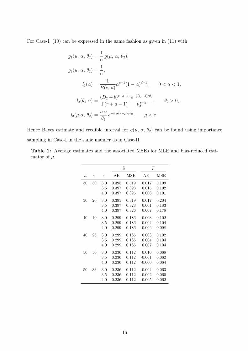
For Case-I, (10) can be expressed in the same fashion as given in (11) with

g1(µ, α, θ2) =1

αg(µ, α, θ2),

g2(µ, α, θ2) =1

α,

l1(α) =1

B(c, d)αc−1(1 − α)d−1, 0 < α < 1,

l2(θ2|α) =(D2 + b)r+a−1

Γ(r + a − 1)

e−(D2+b)/θ2

θ r+a2

, θ2 > 0,

l3(µ|α, θ2) =nα

θ2

e−n α(τ−µ)/θ2 , µ < τ .

Hence Bayes estimate and credible interval for g(µ, α, θ2) can be found using importance

sampling in Case-I in the same manner as in Case-II.

Table 1: Average estimates and the associated MSEs for MLE and bias-reduced esti-mator of µ.

µ µ

n r τ AE MSE AE MSE

30 30 3.0 0.395 0.319 0.017 0.1993.5 0.397 0.323 0.015 0.1924.0 0.397 0.326 0.006 0.191

30 20 3.0 0.395 0.319 0.017 0.2043.5 0.397 0.323 0.001 0.1834.0 0.397 0.326 0.007 0.178

40 40 3.0 0.299 0.186 0.003 0.1023.5 0.299 0.186 0.004 0.1044.0 0.299 0.186 -0.002 0.098

40 26 3.0 0.299 0.186 0.003 0.1023.5 0.299 0.186 0.004 0.1044.0 0.299 0.186 0.007 0.104

50 50 3.0 0.236 0.112 0.010 0.0683.5 0.236 0.112 -0.001 0.0624.0 0.236 0.112 -0.000 0.064

50 33 3.0 0.236 0.112 -0.004 0.0633.5 0.236 0.112 -0.002 0.0604.0 0.236 0.112 0.005 0.062

16

Table 2: Coverage percentages and average lengths of bootstrap and asymptotic confi-dence intervals along with average estimates and the associated MSEs for MLE of θ1.

95% 99%

BCI ACI BCI ACI

n r τ AE MSE CP AL CP AL CP AL CP AL

30 30 3.0 11.962 38.754 92.72 21.315 84.42 20.647 98.38 35.269 91.48 27.1353.5 11.984 33.486 92.36 20.527 86.22 19.134 98.38 34.286 91.66 25.1474.0 11.925 27.370 93.26 19.402 86.62 17.937 98.56 31.918 93.30 23.573

30 20 3.0 11.962 38.754 93.22 21.977 86.18 21.007 98.34 36.415 92.08 27.6073.5 11.984 33.486 93.56 20.231 86.26 18.652 98.66 33.849 93.06 24.5134.0 11.796 22.487 93.12 19.146 87.70 17.515 98.48 31.550 92.98 23.019

40 40 3.0 12.010 27.018 94.02 19.224 87.54 17.418 98.74 32.005 93.52 22.8923.5 11.982 22.815 93.96 17.491 88.72 15.899 98.70 28.649 94.10 20.8944.0 11.767 15.041 93.82 15.956 89.36 14.628 98.82 25.159 94.58 19.224

40 26 3.0 12.010 27.018 93.52 19.110 87.80 17.292 98.92 32.063 93.04 22.7263.5 11.982 22.815 93.54 17.439 88.28 15.782 98.72 28.653 93.66 20.7414.0 11.793 17.007 94.02 16.074 89.18 14.747 98.82 25.389 94.58 19.381

50 50 3.0 11.993 18.326 94.10 16.599 89.28 15.084 98.88 26.894 94.02 19.8243.5 11.968 14.545 94.08 15.250 90.18 13.964 98.72 23.995 94.78 18.3514.0 11.795 11.707 93.34 13.876 89.72 12.922 98.66 20.947 94.82 16.983

50 33 3.0 11.993 18.326 93.62 16.589 88.30 15.039 98.84 26.954 93.66 19.7643.5 11.968 14.545 94.22 15.293 90.10 13.994 98.90 24.077 94.96 18.3914.0 11.900 12.578 93.58 14.107 89.94 13.114 98.84 21.378 94.88 17.235

6 Simulation Results and Data Analysis

To evaluate the performance of the CIs and CRIs we conduct a few simulation studies to

obtain the coverage percentage (CP) and the average length (AL) of the CIs and CRIs of the

different parameters of interest and the median of the first stress level. All the results are

based on 5000 simulations with µ = 0, θ1 = 12, θ2 = 4.5, M = 3000. We consider different

values of n, viz., 30, 40, and 50 and different values for τ , viz., 3.0, 3.5, and 4.0. For each

value of n, we consider r = n and r = 0.65 n. Here we take non-informative priors on all the

parameters, i.e., a = 0, b = 0, c = 1, d = 1 for the Bayesian inference, so that this result

can be compared with that of frequentist approach. Note that Bayes estimate of µ and θ1

exist if N − 1 > 0 and r − 2 > 0, that of θ2 exists if N > 0 and r − 2 > 0. Also note that

we discard those samples for which the Bayes estimate of θ1 and θ2 exceed 100 and those

samples for which Bayes estimate of µ and median of the first stress level either less than

17

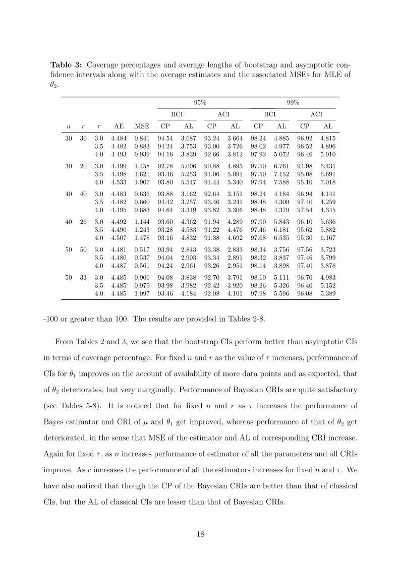
Table 3: Coverage percentages and average lengths of bootstrap and asymptotic con-fidence intervals along with the average estimates and the associated MSEs for MLE ofθ2.

95% 99%

BCI ACI BCI ACI

n r τ AE MSE CP AL CP AL CP AL CP AL

30 30 3.0 4.484 0.841 94.54 3.687 93.24 3.664 98.24 4.885 96.92 4.8153.5 4.482 0.883 94.24 3.753 93.00 3.726 98.02 4.977 96.52 4.8964.0 4.493 0.939 94.16 3.839 92.66 3.812 97.92 5.072 96.46 5.010

30 20 3.0 4.499 1.458 92.78 5.006 90.88 4.893 97.50 6.761 94.98 6.4313.5 4.498 1.621 93.46 5.253 91.06 5.091 97.50 7.152 95.08 6.6914.0 4.533 1.907 93.80 5.547 91.44 5.340 97.94 7.588 95.10 7.018

40 40 3.0 4.483 0.636 93.88 3.162 92.64 3.151 98.24 4.184 96.94 4.1413.5 4.482 0.660 94.42 3.257 93.46 3.241 98.48 4.309 97.40 4.2594.0 4.495 0.683 94.64 3.319 93.82 3.306 98.48 4.379 97.54 4.345

40 26 3.0 4.492 1.144 93.60 4.362 91.94 4.289 97.90 5.843 96.10 5.6363.5 4.490 1.243 93.28 4.583 91.22 4.476 97.46 6.181 95.62 5.8824.0 4.507 1.478 93.16 4.832 91.38 4.692 97.68 6.535 95.30 6.167

50 50 3.0 4.481 0.517 93.94 2.843 93.38 2.833 98.34 3.756 97.56 3.7233.5 4.480 0.537 94.04 2.903 93.34 2.891 98.32 3.837 97.46 3.7994.0 4.487 0.561 94.24 2.961 93.26 2.951 98.14 3.898 97.40 3.878

50 33 3.0 4.485 0.906 94.08 3.838 92.70 3.791 98.10 5.111 96.70 4.9833.5 4.485 0.979 93.98 3.982 92.42 3.920 98.26 5.326 96.40 5.1524.0 4.485 1.097 93.46 4.184 92.08 4.101 97.98 5.596 96.08 5.389

-100 or greater than 100. The results are provided in Tables 2-8.

From Tables 2 and 3, we see that the bootstrap CIs perform better than asymptotic CIs

in terms of coverage percentage. For fixed n and r as the value of τ increases, performance of

CIs for θ1 improves on the account of availability of more data points and as expected, that

of θ2 deteriorates, but very marginally. Performance of Bayesian CRIs are quite satisfactory

(see Tables 5-8). It is noticed that for fixed n and r as τ increases the performance of

Bayes estimator and CRI of µ and θ1 get improved, whereas performance of that of θ2 get

deteriorated, in the sense that MSE of the estimator and AL of corresponding CRI increase.

Again for fixed τ , as n increases performance of estimator of all the parameters and all CRIs

improve. As r increases the performance of all the estimators increases for fixed n and τ . We

have also noticed that though the CP of the Bayesian CRIs are better than that of classical

CIs, but the AL of classical CIs are lesser than that of Bayesian CRIs.

18

Table 4: Coverage percentages and average lengths of bootstrap confidence intervals ofη0.5 along with the average estimates and the associated MSEs of η0.5 as an estimator ofη0.5.

95% 99%

n r τ AE MSE CP AL CP AL

30 30 3.0 8.116 14.353 92.52 14.349 98.84 24.1713.5 8.124 12.938 92.42 13.413 98.34 22.4924.0 8.174 10.834 93.20 12.683 98.58 21.044

30 20 3.0 8.094 14.071 92.36 14.332 98.44 24.1093.5 8.187 13.323 92.72 13.549 98.64 22.7234.0 8.186 9.070 93.30 12.655 98.70 21.049

40 40 3.0 8.233 9.976 93.36 12.622 98.52 20.9603.5 8.225 9.197 93.14 11.590 98.52 18.7574.0 8.219 8.136 93.32 10.779 98.14 16.956

40 26 3.0 8.220 11.055 93.64 12.609 98.54 20.9463.5 8.172 8.165 93.36 11.465 98.60 18.5724.0 8.226 7.254 93.70 10.756 98.76 16.950

50 50 3.0 8.155 8.208 93.70 10.890 98.62 17.3153.5 8.247 6.626 93.92 10.155 98.78 15.7594.0 8.263 5.418 94.26 9.461 98.96 14.314

50 33 3.0 8.272 7.680 93.66 11.103 99.00 17.7343.5 8.234 6.309 93.78 10.125 98.76 15.6584.0 8.177 5.705 93.92 9.334 99.04 14.126

Next we provide a data analysis to illustrate the procedures described in sections 2, 4,

and 5. A artificial data is generated from the CEM given in (2) with n = 30, µ = 10.0,

θ1 = e2.5, θ2 = e1.5, and τ = 14.5 and is given in Table 9. Based on the assumption that the

data given in Table 9 is coming from exponential CEM, MLE of all the three parameters

can be found using (5) and Bayes estimates can be found using the algorithm described in

section 5. Here also we consider two values of r, viz., 30 and 20. For r = 30, MLE of µ, θ1,

θ2 and median of the first stress level are 10.05, 17.22, 3.50, and 21.99 and Bayes estimate

of that are 9.93, 8.52, 5.58, and 23.08 respectively. For r = 20, MLEs are 10.05, 17.21,

3.69, 21.99 and Bayes estimates are 9.89, 11.25, 7.37, and 23.37 respectively. Bias-reduced

estimates of µ and median of the first stress level are same for both values of r and they

are 9.48 and 21.40 respectively. Asymptotic and bootstrap CI, percentile and HPD CRI are

also computed and reported in Table 10.

19

Table 5: Coverage percentages and average lengths of different credible intervals alongwith the average estimates and the associated MSEs for Bayes estimates of µ.

Per. CRI HPD CRI % of

95% 99% 95% 99% samples

n r τ AE MSE CP AL CP AL CP AL CP AL discarded

30 30 3.0 -0.163 1.047 95.58 2.456 99.10 5.190 95.44 1.773 99.18 3.827 0.0003.5 -0.114 0.575 95.46 2.163 98.98 4.168 95.50 1.621 99.00 3.124 0.0004.0 -0.090 0.385 95.46 1.999 98.94 3.619 95.44 1.528 98.98 2.780 0.000

30 20 3.0 -0.182 2.200 95.18 2.510 99.04 5.454 95.62 1.795 99.42 3.913 0.0203.5 -0.106 0.366 95.24 2.141 99.12 3.826 95.72 1.614 99.18 3.028 0.0004.0 -0.076 0.289 95.16 2.006 99.04 3.473 95.50 1.536 99.04 2.745 0.000

40 40 3.0 -0.051 0.130 95.38 1.471 98.94 2.499 94.86 1.132 99.04 2.015 0.0003.5 -0.041 0.130 95.36 1.398 98.98 2.328 95.12 1.087 98.98 1.884 0.0004.0 -0.031 0.110 95.26 1.335 98.90 2.115 94.82 1.048 99.14 1.766 0.000

40 26 3.0 -0.065 0.178 95.62 1.507 99.24 2.593 95.88 1.154 99.26 2.076 0.0003.5 -0.049 0.107 95.34 1.403 99.16 2.276 95.78 1.093 99.24 1.879 0.0004.0 -0.039 0.099 95.32 1.342 99.24 2.127 95.48 1.054 99.20 1.776 0.000

50 50 3.0 -0.036 0.076 94.86 1.087 99.00 1.750 94.92 0.851 98.98 1.455 0.0003.5 -0.028 0.065 94.94 1.042 98.98 1.632 94.80 0.823 98.98 1.370 0.0004.0 -0.024 0.063 94.90 1.017 98.94 1.574 94.80 0.808 99.04 1.328 0.000

50 33 3.0 -0.031 0.073 95.30 1.084 98.78 1.732 94.72 0.850 98.84 1.439 0.0003.5 -0.024 0.070 94.94 1.043 98.74 1.634 94.74 0.823 98.66 1.371 0.0004.0 -0.021 0.067 94.80 1.016 98.70 1.571 94.86 0.807 98.78 1.326 0.000

7 Conclusion

The two-parameter exponential distribution has been considered in a simple step-stress

model. Presence of the common location parameter is justified in the view of possibility

of an unknown bias in the life-time experiment data. We obtain the exact distributions of

the MLEs of the scale parameters at the two stress levels. The exact confidence limits of the

scale parameters are difficult to obtain, due to the complicated nature of the model. We have

proposed to use asymptotic and parametric bootstrap CIs, and the performance of the later

is better. We have further proposed Bayesian inference of the unknown parameters under

fairly general prior assumptions, and we obtained the Bayes estimates and the associated

credible intervals using importance sampling technique. The proposed Bayes estimates and

the credible intervals perform quite well.

20

Table 6: Coverage percentages and average lengths of different credible intervals alongwith the average estimates and the associated MSEs for Bayes estimates of θ1.

Per. CRI HPD CRI % of

95% 99% 95% 99% samples

n r τ AE MSE CP AL CP AL CP AL CP AL discarded

30 30 3.0 15.331 108.646 96.50 32.775 99.66 58.700 94.88 26.657 99.00 47.595 0.3393.5 14.639 84.449 95.70 27.737 99.30 46.712 94.76 23.348 98.98 39.176 0.1404.0 14.092 48.497 95.26 23.792 99.24 37.668 94.44 20.657 98.68 32.754 0.120

30 20 3.0 15.300 95.726 97.04 32.054 99.58 57.465 95.76 26.337 99.24 46.534 0.3793.5 14.733 72.332 96.70 27.527 99.50 46.018 95.90 23.301 99.22 38.804 0.1004.0 14.203 49.417 96.28 23.967 99.54 38.256 95.50 20.796 99.24 33.188 0.080

40 40 3.0 14.016 52.416 95.22 23.452 99.36 37.310 94.08 20.356 99.00 32.333 0.0803.5 13.570 36.284 95.00 20.248 99.38 30.893 94.54 18.025 99.08 27.512 0.0804.0 13.294 28.380 95.28 18.177 99.36 26.995 94.84 16.438 98.90 24.450 0.020

40 26 3.0 14.038 49.181 95.98 23.197 99.46 36.772 95.02 20.198 99.30 31.965 0.1803.5 13.737 37.947 95.90 20.502 99.22 31.311 94.86 18.237 99.12 27.884 0.0404.0 13.410 27.432 95.84 18.223 99.38 27.046 95.02 16.510 99.18 24.518 0.000

50 50 3.0 13.441 31.436 94.92 18.946 99.16 28.454 93.76 17.033 99.00 25.582 0.0203.5 13.144 22.906 95.00 16.741 99.02 24.440 93.96 15.319 98.96 22.394 0.0004.0 12.960 18.053 95.12 15.259 99.04 21.903 94.32 14.126 98.86 20.308 0.000

50 33 3.0 13.435 32.587 95.66 18.839 99.10 28.330 95.04 16.945 99.06 25.469 0.0203.5 13.117 21.933 95.78 16.580 99.26 24.189 94.60 15.180 99.10 22.169 0.0204.0 12.946 17.007 95.76 15.131 99.18 21.737 94.92 14.011 99.12 20.127 0.000

Acknowledgements

The authors would like to thank two reviewers, the associate editor and the editor for their

constructive comments.

Appendix: Lemmas and Proofs of the Theorems

Lemma .1. Let X1:n < · · · < Xn:n be the order statistics of a random sample of size n from

a continuous distribution with PDF f(x). Let D denote the number of order statistics less

than or equal to some pre-fixed number τ , such that F (τ) > 0, where F (.) is the distribution

function of f(.). The conditional joint PDF of X1:n, · · · , XD:n given that D = j is identical

with the joint PDF of all order statistics of size j from the right truncated density function

f∗(t) =

{f(t)F (τ)

for t < τ

0 otherwise.

21

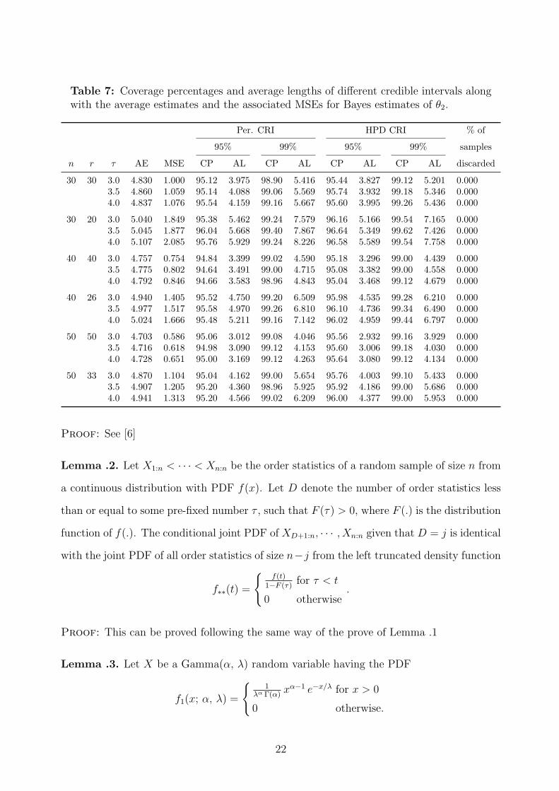
Table 7: Coverage percentages and average lengths of different credible intervals alongwith the average estimates and the associated MSEs for Bayes estimates of θ2.

Per. CRI HPD CRI % of

95% 99% 95% 99% samples

n r τ AE MSE CP AL CP AL CP AL CP AL discarded

30 30 3.0 4.830 1.000 95.12 3.975 98.90 5.416 95.44 3.827 99.12 5.201 0.0003.5 4.860 1.059 95.14 4.088 99.06 5.569 95.74 3.932 99.18 5.346 0.0004.0 4.837 1.076 95.54 4.159 99.16 5.667 95.60 3.995 99.26 5.436 0.000

30 20 3.0 5.040 1.849 95.38 5.462 99.24 7.579 96.16 5.166 99.54 7.165 0.0003.5 5.045 1.877 96.04 5.668 99.40 7.867 96.64 5.349 99.62 7.426 0.0004.0 5.107 2.085 95.76 5.929 99.24 8.226 96.58 5.589 99.54 7.758 0.000

40 40 3.0 4.757 0.754 94.84 3.399 99.02 4.590 95.18 3.296 99.00 4.439 0.0003.5 4.775 0.802 94.64 3.491 99.00 4.715 95.08 3.382 99.00 4.558 0.0004.0 4.792 0.846 94.66 3.583 98.96 4.843 95.04 3.468 99.12 4.679 0.000

40 26 3.0 4.940 1.405 95.52 4.750 99.20 6.509 95.98 4.535 99.28 6.210 0.0003.5 4.977 1.517 95.58 4.970 99.26 6.810 96.10 4.736 99.34 6.490 0.0004.0 5.024 1.666 95.48 5.211 99.16 7.142 96.02 4.959 99.44 6.797 0.000

50 50 3.0 4.703 0.586 95.06 3.012 99.08 4.046 95.56 2.932 99.16 3.929 0.0003.5 4.716 0.618 94.98 3.090 99.12 4.153 95.60 3.006 99.18 4.030 0.0004.0 4.728 0.651 95.00 3.169 99.12 4.263 95.64 3.080 99.12 4.134 0.000

50 33 3.0 4.870 1.104 95.04 4.162 99.00 5.654 95.76 4.003 99.10 5.433 0.0003.5 4.907 1.205 95.20 4.360 98.96 5.925 95.92 4.186 99.00 5.686 0.0004.0 4.941 1.313 95.20 4.566 99.02 6.209 96.00 4.377 99.00 5.953 0.000

Proof: See [6]

Lemma .2. Let X1:n < · · · < Xn:n be the order statistics of a random sample of size n from

a continuous distribution with PDF f(x). Let D denote the number of order statistics less

than or equal to some pre-fixed number τ , such that F (τ) > 0, where F (.) is the distribution

function of f(.). The conditional joint PDF of XD+1:n, · · · , Xn:n given that D = j is identical

with the joint PDF of all order statistics of size n−j from the left truncated density function

f∗∗(t) =

{f(t)

1−F (τ)for τ < t

0 otherwise.

Proof: This can be proved following the same way of the prove of Lemma .1

Lemma .3. Let X be a Gamma(α, λ) random variable having the PDF

f1(x; α, λ) =

{1

λα Γ(α)xα−1 e−x/λ for x > 0

0 otherwise.

22

Table 8: Coverage percentages and average lengths of different credible intervals alongwith the average estimates and the associated MSEs for Bayes estimates of the medianof the first stress level.

Per. CRI HPD CRI % of

95% 99% 95% 99% samples

n r τ AE MSE CP AL CP AL CP AL CP AL discarded

30 30 3.0 10.522 48.677 96.44 21.803 99.60 39.388 95.10 17.746 99.18 31.805 0.3193.5 10.062 37.875 95.86 18.509 99.24 31.308 94.78 15.582 99.06 26.239 0.1204.0 9.741 24.559 95.82 16.037 99.22 25.578 94.54 13.924 98.72 22.173 0.040

30 20 3.0 10.490 42.086 96.76 21.276 99.56 38.104 95.64 17.499 99.14 30.899 0.3793.5 10.115 31.838 96.68 18.289 99.44 30.562 95.70 15.502 99.22 25.828 0.1004.0 9.810 24.366 96.74 16.108 99.44 25.829 95.60 13.974 99.24 22.394 0.020

40 40 3.0 9.708 26.357 95.34 15.918 99.42 25.432 94.54 13.792 98.90 22.015 0.0203.5 9.409 19.095 95.20 13.776 99.32 21.176 94.26 12.238 99.02 18.788 0.0204.0 9.200 13.898 95.46 12.290 99.22 18.308 94.74 11.105 98.98 16.571 0.000

40 26 3.0 9.741 26.678 96.00 15.849 99.48 25.395 95.22 13.765 99.36 21.993 0.0803.5 9.506 19.604 95.92 13.908 99.22 21.371 94.88 12.350 99.08 18.960 0.0004.0 9.256 12.392 95.86 12.256 99.36 18.195 95.18 11.115 99.16 16.502 0.000

50 50 3.0 9.282 14.385 95.06 12.804 99.16 19.223 93.82 11.518 99.02 17.296 0.0203.5 9.083 10.457 95.42 11.322 98.92 16.529 93.88 10.367 98.82 15.151 0.0004.0 8.959 8.250 95.04 10.328 98.98 14.827 94.30 9.567 98.86 13.751 0.000

50 33 3.0 9.298 16.137 95.62 12.794 99.02 19.308 95.06 11.502 99.04 17.331 0.0003.5 9.068 10.032 95.90 11.212 99.22 16.363 94.78 10.270 99.08 15.001 0.0204.0 8.953 7.806 95.84 10.240 99.18 14.715 95.14 9.487 99.10 13.631 0.000

Then for any arbitrary constant A, the MGF of A + X is given by

MA+X = eA ω (1 − λ ω)−α for ω < 1λ

Proof: It can be proved by simple integration and hence the proof is omitted.

Lemma .4. Let X be an Exponential(λ) random variable having PDF

f2(y; λ) =

{e−y for y > 0

0 otherwise.

Then for any arbitrary constant A, the MGF of A − X is given by

MA−X (ω) = eωA (1 + λ ω)−1 for ω > −1

λ.

Proof: It can be proved by simple integration and hence the proof is omitted.

23

Table 9: Data for illustrative example.

Stress level Data

110.05 10.59 12.73 12.99 13.71 14.0314.34

2

14.53 14.97 15.37 15.43 15.48 15.6015.76 16.18 16.46 16.86 16.90 17.0217.36 17.62 18.06 18.31 18.69 18.9418.95 22.65 22.89 24.51 25.39

Table 10: Results of data analysis.

Type of µ θ1 θ2 Median

r CI/CRI LL UL LL UL LL UL LL UL

95% 30 ACI – – 4.46 29.95 2.07 4.93 – –BCI – – 7.39 20.70 2.24 4.32 15.47 36.77Per. CRI 9.89 9.96 6.54 11.10 4.29 7.27 16.15 36.59HPD CRI 9.90 9.96 6.34 10.76 4.15 7.05 14.47 32.68

20 ACI – – 4.46 29.95 1.69 5.70 – –BCI – – 7.39 20.70 2.09 5.27 15.47 36.77Per. CRI 9.84 9.94 8.15 14.78 5.34 9.69 16.16 37.74HPD CRI 9.84 9.93 8.28 14.84 5.43 9.73 15.10 34.21

99% 30 ACI – – 0.45 33.96 1.62 5.38 – –BCI – – 6.27 23.62 2.07 4.83 14.32 51.85Per. CRI 9.88 9.97 5.86 12.10 3.84 7.94 15.12 50.11HPD CRI 9.89 9.97 5.70 11.68 3.73 7.66 14.35 43.59

20 ACI – – 0.45 33.96 1.05 6.33 – –BCI – – 6.27 23.62 1.90 5.90 14.32 51.85Per. CRI 9.83 9.95 7.30 15.52 4.78 10.17 15.14 48.41HPD CRI 9.83 9.94 7.59 15.55 4.97 10.19 13.74 43.31

Corollary .1. Let X be a Gamma(α, λ1) random variable, Y be an Exponential(λ2) random

variable and they are independently distributed. Then for any arbitrary constant A, the

MGF of A + X − Y is

MA+X−Y (ω) = eωA (1 − λ1 ω)−α (1 + λ2 ω)−1 for −1

λ2

< ω <1

λ1

.

Proof: Using Lemmas .3 and .4, it can be proved easily.

Lemma .5. Let X be a Gamma(α, λ1), Y an Exponential(λ2) random variable and they

are independently distributed. Then the PDF of X − Y is given by

f(t; α, λ1, λ2) =1

λα1 λ2 Γ(α)

et/λ2

∫ ∞

max{0,t}zα−1e

−( 1

λ1+ 1

λ2)z

dz for t ∈ R.

24

Proof: It can be proved using transformation of variable.

Proof of Theorem 3.1:

Using the lemma .1, we get

E[eω bθ1 |N = 1] =1

θ1

(1 − e

− τ−µθ1

)∫ τ

µ

eω(t1−nt1+(n−1)τ)− 1

θ1(t1−µ)

dt1

=e− 1

θ1(τ−µ)

θ1

(1 − e

− τ−µθ1

)∫ τ

µ

e

“ωn−ω+ 1

θ1

”(t1−τ)

dt1

=e− 1

θ1(τ−µ)

θ1

(1 − e

− τ−µθ1

) ×e

“ωn−ω+ 1

θ1

”(τ−µ)

− 1

ωn − ω + 1θ1

. (12)

Using the lemma .1, we get for i = 2(1) r − 1

E[eω bθ1|N = i] =i!

θi1

(1 − e

− τ−µθ1

)i

×

∫ τ

µ

∫ τ

t1

· · ·

∫ τ

ti−2

∫ τ

ti−1

eωi(Pi

j=1 tj−nt1+(n−i)τ)− 1

θ1

Pij=1(tj−µ)

dti · · · dt1

=i!e

− iθ1

(τ−µ)

θi1

(1 − e

− τ−µθ1

)i

×

∫ τ

µ

∫ τ

t1

· · ·

∫ τ

ti−2

∫ τ

ti−1

e−

“ωni−ω

i+ 1

θ1

”(t1−τ)−

“1

θ1−ω

i

” Pij=2(tj−τ)

dti · · · dt1

=

(1

θ1

−ω

i

)−1 ∫ τ

µ

· · ·

∫ τ

ti−2

e−

“ωni−ω

i+ 1

θ1

”(t1−µ)−

“1

θ1−ω

i

” Pi−1j=2

(tj−τ)

×

{e−

“1

θ1−ω

i

”(ti−1−τ)

− 1

}dti−1 · · · dt1

...

=e− i

θ1(τ−µ)

(1 − e

− 1

θ1(τ−µ)

)i

i−1∑

j=0

(−1)i−j−1

(i

j + 1

)e

nωi(n−j−1)+ 1

θ1(j+1)

o(τ−µ)

− 1(1 − ω θ1

i

)i−1(1 + ω(n−j−1)θ1

j(i+1)

) .

(13)

25

Hence using (7), (12), and (13), we have

M1(ω|A) =r−1∑

i=1

i−1∑

j=0

(−1)i−j−1

∑n−1k=1 pk

(n

i

)(i

j + 1

)e− n

θ1(τ−µ) e

nωi(n−j−1)+ 1

θ1(j+1)

o(τ−µ)

− 1(1 − ωθ1

i

)i−1(1 + ω(n−j−1)θ1

i(j+1)

)

=r−1∑

i=1

i−1∑

j=0

cijeωτij

(1 − θ1ω

i

)i−1(1 + (n−j−1)θ1ω

(j+1)i

)

−

r−1∑

i=1

i−1∑

j=0

dij1

(1 − θ1ω

i

)i−1(1 + (n−j−1)θ1ω

(j+1)i

) .

where τij, cij and dij are defined in (9). Now using Lemmas .3, .5 and Corollary .1, we have

(8) and this completes the proof of the Theorem 3.1.

Proof of Theorem 3.2

CMGF of θ2 can be expressed as

E[eω bθ2|1 ≤ N ≤ r − 1] =r−1∑

i=1

E[eω bθ2 |N = i] × P (N = i|1 ≤ N ≤ r − 1).

Using Lemma .2, for i = 1, 2, · · · , r − 1

E[eω bθ2 |N = i] =(n − i)!

(n − r)! θr−i2

e−

“ω

r−i− 1

θ2

”(n−i)τ

×

∫ ∞

τ

∫ ∞

ti+1

· · ·

∫ ∞

tn−1

e−Pr−1

j=i+1

“1

θ2− ω

r−i

”tj:n−

“1

θ2− ω

r−i

”(n−r+1)tr:ndtn · · · dti+1

=1

(1 − θ2 ω

r−i

)r−i .

Therefore

E[eω bθ2|1 ≤ N ≤ r − 1] =r−1∑

i=1

1(1 − θ2 ω

r−i

)r−i ×pi∑r−1

k=1 pk

.

Using the Lemma .3, we have the Theorem 3.2.

References

[1] Bagdonavicius, V. (1978), “Testing the hypothesis of the additive accumulation of dam-

ages”, Probability Theory and its Applications, vol 23, 403–408.

26

[2] Bagdonavicius, V. and Nikulin, M. (2001), “Mathematical models in the theory of

accelerated experiments”, In: Mathematics and the 21st century, Singapore, World

Scientific, Eds Ashor A. A. and Obada A. S. F., 271–303.

[3] Bagdonavicius, V. B. and Nikulin, M. (2002), “Accelerated life models: modeling and

statistical analysis”, Chapman and Hall/ CRC Press, Boca Raton, Florida.

[4] Bagdonavicius, V., Nikulin, M., and Reache, L. (2002), “ On parametric inference for

step-stresses models”, IEEE Transaction on Reliability, vol 51, 27–31.

[5] Balakrishnan, N. (2009), “A synthesis of exact inferential results for exponential step-

stress models and associated optimal accelerated life-tests”, Metrika, vol. 69, 351 - 396.

[6] Balakrishnan, N., Kundu, D., Ng, H.K.T. and Kannan, N. (2007), “Point and interval

estimation for a simple step-stress model with type-II censoring”, Journal of Quality

Technology, vol. 39, 35 - 47.

[7] Bhattacharyya, G. K. and Soejoeti, Z. (1989), “A tempered failure rate model for step-

stress accelerated life test”, Communications in Statistics - Theory and Methods, vol

18, 1627–1643.

[8] Chen, S. M. and Bhattacharyya, G.K. (1988), “Exact confidence bound for an expo-

nential parameter under hybrid censoring”, Communication in Statistics, Theory and

Methods, vol 16, 1857-1870.

[9] Cox, D. R. (1972), “Regression models and life tables”, Journal of the Royal Statistical

Society. Series B (Methodological), vol 34, 187–220.

[10] Bartholmew, D.J. (1963), “The sampling distribution of an estimate arising in life-

testing”, Technometrics, vol. 5, 361 - 372.

[11] DeGroot, M.H. and Goel, P.K. (1979), “Bayesian estimation and optimal design in

partially accelerated life testing”, Naval Research Logistics Quarterly, vol. 26, 223 - 235.

27

[12] Dorp, J. R., Mazzuchi T. A., Fornell, G E, and Pollock, L. R. (1996). “A Bayes approach

to step-stress accelerated life testing”. IEEE Transactions on Reliability, vol. 45, 491-

498.

[13] Efron, B and Liberian, R. (1993), “An Introduction to the bootstrap”, Chapman &

Hall, New York.

[14] Fan, T. H., Wang, E. L., and Balakrishnan, N. (2008), “Exponential progressive step-

stress life-testing with link function based on Box-Cox transformation”, Journal of Sta-

tistical Planing and Inference, vol. 138, 2340 - 2354.

[15] Gerville-Reache, L. and Nikulin, M. (2007), “Some recent results on accelerated failure

time models with time-varying stresses”, Quality Technology and Quantitative Manage-

ment, vol 4, 143–155.

[16] Lee, J. and Pan, R, (2008), “Bayesian inference model for step-stress accelerated life

testing with Type-II censoring”, Reliability and Maintainability Symposium, 91 - 96.

[17] Lee, J. and Pan, R. (2011), “Bayesian analysis of step-stress accelerated life test

with exponential distribution”, Quality and Reliability Engineering International, DOI:

10.1002/qre.1251.

[18] Leu, L. Y. and Shen, K. F. (2007), “Bayesian approach for optimum step-stress accel-

erated life testing”, Journal of Chinese Statistical Association, vol. 45, 221 - 225

[19] Lindley, D.V. (1980), “ Approximate Bayesian Methods”, Trabajos de Estadsticay de

Investigacin Operativa, vol. 31, No. 1, 223 - 245.

[20] Meeker, W.Q. and Escobar, L.A. (1998), Statistical methods for reliability data, John

Wiley and Sons, New York.

[21] Miller, R. and Nelson, W.B. (1983), “Optimum simple step-stress plans for accelerated

life testing”, IEEE Transactions on Reliability, vol. 32, 59 - 65.

28

[22] Nelson, W.B. (1980), “Accelerated life testing: step-stress models and data analysis”,

IEEE Transactions on Reliability, vol. 29, 103 - 108.

[23] Nelson, W.B. (1990), Accelerated life testing, statistical models, test plans and data

analysis, John Wiley and Sons, New York.

[24] Ramadan, S. Z. and Ramadan, K. Z. (2012) “Bayesian simple stepstress acceleration life

testing plan under progressive Type-I right censoring for exponential life distribution”,

Modern Applied Science, vol. 6, 91 - 99.

[25] Sedyakin, N.M. (1966), “On one physical principle in reliability theory”, Technical Cy-

bernatics, vol. 3, 80 - 87.

[26] Shao, J. and Tu, D. (1995), The Jackknife and Bootstrap, Springer, New York.

[27] Xiong, C. (1998) Inference on a simple step-stress model with Type-II censored expo-

nential data, IEEE Transactions on Reliability, Vol.-47, 142-146.

[28] Xiong, C. and Milliken, G.A. (1999), “Step-stress life testing with random stress chang-

ing times for exponential data”, IEEE Transactions on Reliability, vol. 48, 141 - 148.

29