on shape-preserving wavelet estimators of cumulative distribution functions and densities

This article was downloaded by: [Universitätsbibliothek Bern]On: 16 August 2014, At: 06:10Publisher: Taylor & FrancisInforma Ltd Registered in England and Wales Registered Number: 1072954 Registeredoffice: Mortimer House, 37-41 Mortimer Street, London W1T 3JH, UK

Stochastic Analysis and ApplicationsPublication details, including instructions for authors andsubscription information:http://www.tandfonline.com/loi/lsaa20

On shape-preserving waveletestimators of cumulative distributionfunctions and densitiesLubomir Dechevsky a & Spiridon Penev ba Institute of Mathematics and Informatics , Technical UniversitySofia , Sofia, 1156, Bulgariab School of Mathematics Department of Statistics , TheUniversity of New South Wales , Sydney, NSW, 2052, AustraliaPublished online: 03 Apr 2007.

To cite this article: Lubomir Dechevsky & Spiridon Penev (1998) On shape-preserving waveletestimators of cumulative distribution functions and densities, Stochastic Analysis andApplications, 16:3, 423-462

To link to this article: http://dx.doi.org/10.1080/07362999808809543

PLEASE SCROLL DOWN FOR ARTICLE

Taylor & Francis makes every effort to ensure the accuracy of all the information (the“Content”) contained in the publications on our platform. However, Taylor & Francis,our agents, and our licensors make no representations or warranties whatsoever as tothe accuracy, completeness, or suitability for any purpose of the Content. Any opinionsand views expressed in this publication are the opinions and views of the authors,and are not the views of or endorsed by Taylor & Francis. The accuracy of the Contentshould not be relied upon and should be independently verified with primary sourcesof information. Taylor and Francis shall not be liable for any losses, actions, claims,proceedings, demands, costs, expenses, damages, and other liabilities whatsoeveror howsoever caused arising directly or indirectly in connection with, in relation to orarising out of the use of the Content.

This article may be used for research, teaching, and private study purposes. Anysubstantial or systematic reproduction, redistribution, reselling, loan, sub-licensing,systematic supply, or distribution in any form to anyone is expressly forbidden. Terms& Conditions of access and use can be found at http://www.tandfonline.com/page/terms-and-conditions

http://www.tandfonline.com/loi/lsaa20

http://dx.doi.org/10.1080/07362999808809543

http://www.tandfonline.com/page/terms-and-conditions

http://www.tandfonline.com/page/terms-and-conditions

STOCHASTIC ANALYSIS AND APPLICATIONS, 16(3), 423-462 (1998)

ON SHAPE-PRESERVING WAVELET ESTIMATORS OF

CUMULATIVE DISTRIBUTION FUNCTIONS AND DENSITIES

Lubomir Dechevsky

Institute of Mathematics and Informatics, Technical University, Sofia 1 156 Sofia, Bulgaria

Spiridon Penev

School of Mathematics, Department of Statistics

The University of New South Wales

Sydney 2052 NSW, Australia

ABSTRACT

In a previous paper we introduced a general class of shape- preserving wavelet approximating operators (approximators) which transform cumulative distribution functions (cdf) and densities into functions of the same type. Empirical versions of these operators are used in this paper to introduce, in an unified way, shape- preserving wavelet estimators of cdf and densities, with a priori prescribed smoothness properties. We evaluate their risk for a variety of loss functions and analyze their asymptotic behavior. We study the convergence rates depending on minimal additional assumptions about the cdf/ density. These assumptions are in terms of the function belonging to certain homogeneous Besov or Triebel- Lizorkin spaces and others. As a main evaluation tool the integral p-modulus of smoothness is used.

0. PRELIMINARIES -

In this section we collect some preliminary notations and

statements which will be used in the next sections.

Copyright 0 1998 by Marcel Dekker, Inc.

Dow

nloa

ded

by [

Uni

vers

itäts

bibl

ioth

ek B

ern]

at 0

6:10

16

Aug

ust 2

014

DECHEVSKY AND PENEV

For O<p<m and for a Lebesgue- measurable function f : R 4 we denote +m

11flL II= ( 1 ( f ( ~ ) ( ~ d x ) " ~ and ilflLWil= es s sup lf(r)l. If O<pLm , LJR) P

.m X€ R

is the set {f: llf J L ll<m). L is a quasi-Banach space for O<pLm (see P P

[2]) with an embedding constant in the quasi-triangle inequality c =max P

(1 ,21 'P1) : Ilf+glL 11Sc (llflL Il+llglL I[), and, in particular, L is a P P P P P

Banach space for llp5m.

We denote by L,,,oc={f: f 1 p L , ( C ) for every compact C a ) where f l C is the restriction of f on C. The spaces ACloc of (locally) absolutely

continuous functions are defined by ACloc={f~Ll,loc: there exists the

derivative f Lebesgue almost everywhere and f E L,,,m}. As usual,

6'' denotes the v-th derivative of a univariate function f. For

fe LIJoc, p~ N, O<h<m, the Steklov's function (Steklov-means) f is

defined for example in [15],[6]. PJ'

+-J Vf will denote the usual variation of a function f in (-m,+m).

-00

b

We shall also use the notation Vf for the variation in [a,b), 3.

+m -.oLa3<+=. For 15p<-~, V f= V f is the Wiener- Young variation of f.

. m P P

We shall denote by BV the space of functions with a bounded Wiener- P

Young variation V f. Then BVI is the space of functions with bounded P

variation in the usual sense. The homogeneous Sobolev spaces are

. P . C1 (P) defined by W (R)= {f:R-, llfl W ll=llf ( L II<-J}, p ~ ~ , l l p l m . Their P P P

inhomogeneous analogs are defined by

The homogeneous Besov and Triebel- Lizorkin spaces BS and F' W 9'

SEE?, O<p,q+ respectively, as well as their inhomogeneous analogs B W

and FS are defined in [2] , [7], or [18]. Here we only make few notes Pq

for the sake of the reader's orientation. If the homogeneous spaces

BL, P' are defined using Wiener- Paley's theory (via Peetre's W

function ([2], [l8]) or Calderon's function ([7]) as a basis for their Dow

nloa

ded

by [

Uni

vers

itäts

bibl

ioth

ek B

ern]

at 0

6:10

16

Aug

ust 2

014

SHAPE-PRESERVING WAVELET ESTIMATORS

atomic decomposition), then a factorization is carried out modulo

polynomials orthogonal to the concretely chosen Calderon's function

(with respective modification for Peetre's function). The factor-

spaces obtained are independent of the concrete choice of Calderon's

(Peetre's) function and are quasi-Banach spaces (Banach spaces for

l<min(p,q)<~). It is convenient to consider the elements of these

spaces as functions rather than as equivalent classes of functions and,

for a fixed choice of Calderon's (Peetre's) function, consider B"' w' W

to be (quasi-) seminosmed.

1 1 1 For s>max{-,1) -1, respectively s> max{-,-,l}- 1, the Besov, P P 9

respectively Triebel- Lizorkin spaces admit equivalent (quasi-) norms

via finite differences and functional moduli of smoothness. The above

restrictions on s are essential and are related to the fact that for

these ranges of parameters the Besov and Triebel- Lizorkin spaces are

1 contained in L,,,oc. Other important ranges of parameters are s>-, P

1 1 respectively s> max{--1. Then each element (equivalence class) of the p'q

Besov, respectively Triebel- Lizorkin space is (contains) a continuous

function.

The inhomogeneous versions BS F" are quasi-Banach spaces w' W

(Banach spaces for llmin{p,q]+). It is important that for

1 . S . S . s S S

F ~ = L P ~ . For p=q: F =B F =B (with s>max{-, 1)- 1 : B' =LP' P W w w ' w w

equivalent quasi-norms). If pfq, S E R then the Besov and Triebel-

Lizorkin spaces are essentially diverse (see for example [IS]). Many

of the well- known function spaces can be identified as homogeneous or

inhomogeneous Besov or Triebel- Lizorkin spaces for specific values of

p,q and s. For an orientation we refer to [7] and [IS].

For the definition and relevant properties of the Riesz potential

ISf, SEW, we refer to [ 2 ] .

Let h>O, ye N. Denote by o (f,h) (llp5-) the integral p- modulus P p

of smoothness of f. The latter is defined by:

Dow

nloa

ded

by [

Uni

vers

itäts

bibl

ioth

ek B

ern]

at 0

6:10

16

Aug

ust 2

014

DECHEVSKY AND PENEV

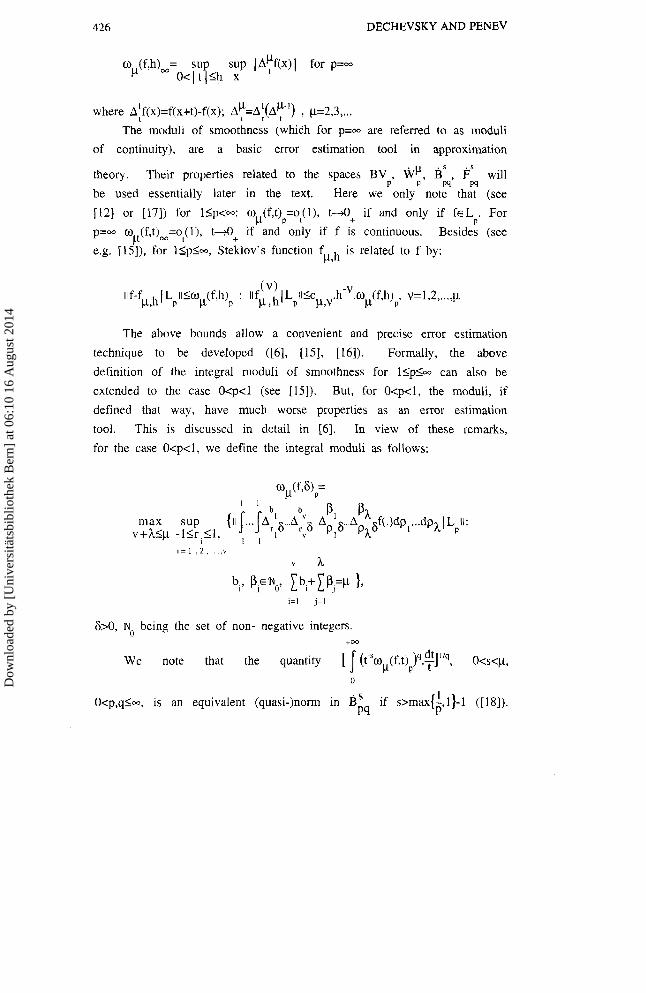
w (f,h)_= sup sup 1 ~ y f ( x ) 1 for p=w O < [ t l l h x

1 p-I where A:f(x)=f(x+t)-f(x); A ~ = A ~ ( A ) . p=2,3 ,.,, The moduli of smoothness (which for p=m are referred to as moduli

of continuity), are a basic error estimation tool in approximation

theory. Their properties related to the spaces BV , wp, B~ , F' will P P W W

be used essentially later in the text. Here we only note that (see

1121 or [ I l l ) for l<.p<m: w (f,t) =ot(l), t 4 + if and only if EL . For I.1 P P

p = ~ w (f,t)m=o (1)' t f O + if and only if f is continuous. Besides (see I'

e.g. [IS]), for ILpSw, Steklov's function f is related to f by: P3h

The above bounds allow a convenient and precise error estimation

technique to be developed ([6], [15], [16]). Formally, the above

definition of the integral moduli of smoothness for 15pS.o can also be

extended to the case Ocp<l (see [15]). But, for Ocp<l, the moduli, if

defined that way, have much worse properties as an error estimation

tool. This is discussed in detail in [6]. In view of these remarks,

for the case O<p<l, we define the integral moduli as follows:

6>0, M being the set of non- negative integers. 0

+w

We note that the quantity q dt l/q [ J t S I , o ~ c p ,

0

1 O<p,qlw, is an equivalent (quasi-)norm in BS if s>rnax{-,l}-1 ([18]). P4 P

Dow

nloa

ded

by [

Uni

vers

itäts

bibl

ioth

ek B

ern]

at 0

6:10

16

Aug

ust 2

014

SHAPE-PRESERVING WAVELET ESTIMATORS 427

t"J

dt 'Iq is an equivalent (quasi-)norm in Also, llf 1 L P it+[ 1 (t-'w,,,(f,t)dg

0

1 B V f s>max{-,l)-1. For the new definition of the integral modulus of W P

smoothness we gave in the case O<p<l, it is possible to show that,

first, it is equivalent to the old one for 1 5 p G ([6]). Next, similar

to the previous definition (see [18]), for w (f,h) it holds in case +m

CL P

1 O<p= qc l and - -l<s <p that [ ( ( t $]'" is an equivalent P C1

0

S S

quasi-norm in i; =B (which equally implies PP PP

o ( ~ , ~ ) ~ C ( ~ , ~ , ~ ) . S . I I ~ ( B ' I I for all f ~ ~ b ) . Finally, for this P p PP

definition a version of the inequalities involving Steklov's function

and its derivatives can be derived also for the case O<p<l (see [6]).

We shall also make use of some facts about concave majorants of

moduli of smoothness. Let F be a continuous function on R. It is a

well- known fact (which can be found in numerous sources on

approximation theory) that W ~ ( F , ~ ) ~ has a "least concave majorant"

wF(t), i.e., ~ , ( F , t ) ~ 6 wF(t), te[O,w), where oFeQ, Q= {a: [O ,w) i

[O,w), w- concave on [O,M), l i m o(t)=w(0)=0), and for every W G R such tie,

that W ~ ( F , ~ ) ~ _ < ~ ~ ( t ) , t~ [Op), it follows that wF(t)<w(t), t t [O,m).

(The idea behind the construction of wF is not difficult to comprehend.

Indeed, let T (~)={(~ ,X)EIR~ : t~[O,m), xsY(t)) be the subgraph of

y(t)=w1(F,t) t t [Op), and denote by ar(y)={(t,y)sR2: t e [ O , ~ ) , ~ = ~ ( t ) }

the graph of y(t). Then the graph of wF(t) is ~ [ F ( Y ) ~ ] , where [ r ( y ) ' ]

is the closure of the convex hull of F(y)). It is easy to verify the

following properties of any o~ Q:

i) o is continuous on [O,m);

ii) if o is not identically 0 on [O,m), then there exists

tw~(O,m], such that w(t) is strictly increasing on [O,tm),

w(t)=m(t,)= sup w(Q t~ [to,-) (the last interval being 0 if to=+-). .tE [OP)

Note that if ~ E R is the least concave majorant of W , ( F , ~ ) ~ , then

Dow

nloa

ded

by [

Uni

vers

itäts

bibl

ioth

ek B

ern]

at 0

6:10

16

Aug

ust 2

014

428 DECHEVSKY AND PENEV

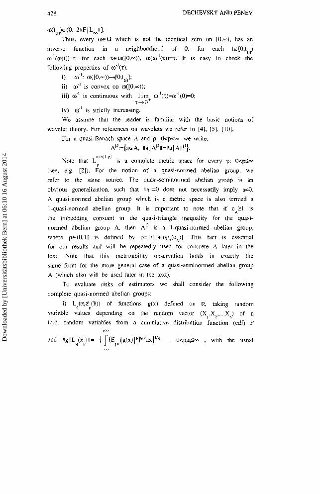
o ( t W ) ~ (0, 211FILmll].

Thus, every w€R which is not the identical zero on [ O p ) , has an

inverse function in a neighbourhood of 0: for each t ~ [ O , t ~ )

w-'(o(t))=t; for each TEW([O,~~)), w(~-~(T) )=T. It is easy to check the

following properties of o.Y1(t):

i) w'l : w([O,-))+[O,t,];

ii) o-I is convex on o([O,w));

iii) o-' is continuous with 1 im ~~Y'(.t)=wl(0)=0; T+O+

iv) o-' is strictly increasing.

We assume that the reader is familiar with the basic notions of

wavelet theory. For references on wavelets we refer to [4], [S], [lo].

For a quasi-Banach space A and p: O<p<-, we write:

AP:={a,A, I I ~ ~ A P I I = I I ~ ~ A I I P } . min(1.p) .

Note that L 1s a complete metric space for every p: O<p<w P

(see, e.g. [ 2 ] ) . For the notion of a quasi-normed abelian group, we

refer to the same source. The quasi-seminormed abelian group is an

obvious generalization, such that llall=O does not necessarily imply a=O.

A quasi-normed abelian group which is a metric space is also termed a

I-quasi-normed abelian group. It is important to note that if c 21 is A

the imbedding constant in the quasi-triangle inequality for the quasi-

normed abelian group A, then A~ is a 1-quasi-normed abelian group,

where p ~ ( 0 , 1 ] is defined by p=ll[l+log2(cA)]. This fact is essential

for our results and will be repeatedly used for concrete A later in the

text. Note that this metrizability observation holds in exactly the

same form for the more general case of a quasi-seminormed abelian group

A (which also will be used later in the text).

To evaluate risks of estimators we shall consider the following

complete quasi-normed abelian groups:

i) L4(~,2P(R)) of functions g(x) defined on [R, taking random

variable values depending on the random vector (X ,X2,...,X ) of n 1 n

i.i.d. random variables from a cumulative distribution function (cdf) F +m

and llg(L ( 2 Ill= { I(E (g(x)(')"dr}'" . O<p,q<= . with the usual 9 P Fn

.w

Dow

nloa

ded

by [

Uni

vers

itäts

bibl

ioth

ek B

ern]

at 0

6:10

16

Aug

ust 2

014


ess sup- definition for p = ~ andor q=-. ii) 1 ([R,L (R)) of trajectories of stochastic processes G(x), X E ~

P 9 based on measurable transformations of the random vector (X1,X 2,...,Xn)

of n i.i.d. random variables from a cdf F and IIGI%?(L)fl= P 'l

+m

{E( I G(x) 1 qd~)p'q}'lp, O<p,q+. .m

We note the following facts:

i)for Ilp,q+ , L (2 ) and 1 ( L ) are Banach spaces. For O<p<l 9 P P 4

andor O<q<l, these are quasi- Banach spaces. The embedding constant in

the quasi- triangle inequality for both L ( 1 ) and 1 (L ) is P P 4

c =c c = mar { I ,2"lp7' .maxi 1 / . W P 4

ii)L ( 1 lP and 1 (L )P are 1- quasi- normed for pp* such that 4 P P 9

1 1 1 1 1 --= max(1,-, -, - + - - I ] . P P 9 P 9

iii)in view of the generalized Minkowski's Inequality,

L (2 ) c 2 (L ) for O<q<pIm; 1 (L )cL ( 1 ) for O<plq<m. Here and in the 4 P P Y P 4 4 P

sequel, " A d " , when applied to quasi- seminormed spaces A and B, has

the meaning of continuous imbedding (see [Z], [IS]). For such A and B,

A@ is the intersection of the two spaces with quasi- seminorm

I I ~ ( A ~ B I I = ~ ~ X { I I ~ ~ A I I , I I ~ I B I ~ ) . and A+B is the sum of the two spaces with

quasi-seminorm

llfJA+Bll= inf {llf,l~ll+llf~ IBII} f=f,+f f o~ A,f, E B

For t~ ( 0 , ~ ) the K- functional of Peetre (see, e.g., [13]) is

defined by:

K(t,f;A,B)= i nf (llfolAll+ t.llfl ~ B I I ) f=fo+f ,foe A,f E B

Clearly it is an equivalent quasi-seminorm in A+B and

I I a I A+B ll=K(l ,a;A,B).

In the particular case p=q, by Fubini's theorem, L ( 1 )= 1 (L ) is P P P P

the corresponding L space with tensor- product measure. In this case P

p*=min{l,p]. It is also easily seen that the embedding constant of the

quasi-triangle inequality for (L ( 1 ))P and ( 1 (L ))P is 4 P P Y D

ownl

oade

d by

[U

nive

rsitä

tsbi

blio

thek

Ber

n] a

t 06:

10 1

6 A

ugus

t 201

4

DECHEVSKY AND PENEV

1. INTRODUCTION -

Wavelet methods are becoming increasingly popular in both

approximation theory and probability theory. The classical problem of

estimating cumulative distribution functions (cdf) and/or densities

offers a nice possibility to marry the methods of these theories to

gain a new insight into the quality of estimation of cdf and densities.

Our framework allows to demonstrate the close links between smoothness

of the cdfldensity, tail behavior, rate of convergence and level of

resolution when using wavelet- based estimators.

This paper can be viewed as a continuation of [6]. In the latter

paper we introduced a general class of shape- preserving wavelet

approximating operators (approximators) and analyzed their

approximation properties under minimal assumptions about the regularity

of the cdfldensity. As a main approximation tool the integral p-

modulus of smoothness is used.

In this paper we introduce, as empirical versions of these

approximators, shape- preserving wavelet estimators with an a priori

prescribed smoothness properties. An estimator of a cdfldensity is

defined to be shape-preserving if the estimator is itself a

cdfldensity. The desirability of the shape-preserving property is

obvious. At the same time, one has to add that unless special care is

taken when constructing the estimator this property will often be

violated.

We evaluate the risks of out estimators for a variety of losses

and analyze their asymptotic behavior. If F is a cdf and Ak is the

shape- preserving wavelet approximator defined in (2.1.1) then for a

sample x,,x2, ..., x from F we define ~:"'(F)(X)=A~(;~)(X) to be the A

wavelet estimator of F where Fn is the empirical distribution

function. The objective is to evaluate the risk II~:"'(F)-FI L ( 2 ) I IP (or 4 P

11 A~'(F)-F 1 2 (L ) 11 p, for O<pcm, O<c+ and some p appropriately chosen P P

so that to mmimize the increase of the imbedding constants in the

evaluation due to applications of the quasi- triangle inequalities (see

the Preliminaries). As usual this is done by breaking the risk into a

stochastic and a bias term by applying the (quasi-) triangle

Dow

nloa

ded

by [

Uni

vers

itäts

bibl

ioth

ek B

ern]

at 0

6:10

16

Aug

ust 2

014


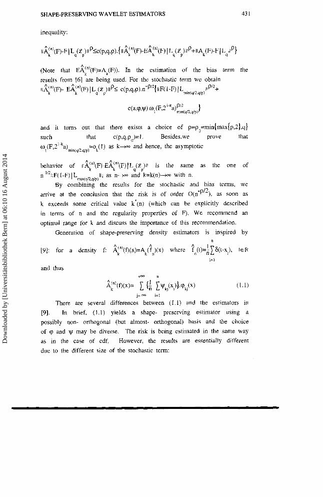
inequality:

(Note that E~~F(F)=A~(F)). In the estimation of the bias term the

results from [6] are being used. For the stochastic term we obtain

II~~;'(F)- E ~ ? ( F ) ( ~ 9 ( & ? ~ ) IIP< C ( ~ , ~ , ~ ) . ~ - ~ ' ~ { I I F ( I - F ) I L mln(q12,qlp) . l1Pn+

and it turns out that there exists a choice of p=p =min{rna~{~,2},~) 0

such that c(p,q,po)=l. Besides,we prove that

=ok(l) as k - ~ and hence, the asymptotic

behavior of II~:"'(F)-E~:")(F)(L~(~JII is the same as the one of

n - 1 1 2 ~ ~ ~ ( l - ~ ) ILmlnlq122q,P)ll, as n- and k=k(n)i.. with n.

By combining the results for the stochastic and bias terms, we

arrive at the conclusion that the risk is of order ~ ( n - ~ ' ~ ) , as soon as

k exceeds some critical value k*(n) (which can be explicitly described

in terms of n and the regularity properties of F). We recommend an

optimal range for k and discuss the importance of this recommendation.

Generation of shape-preserving density estimators is inspired by n

A 1 [91: for a density f: i ~ " ( f ) ( x ) = ~ ~ ( ? ~ ( x ) where fn(t)zE 1 &(t-xi), t~ R

and thus

j=-m i=l

There are several differences between (1.1) and the estimators in

[9] . In brief, (1.1) yields a shape- preserving estimator using a

possibly non- orthogonal (but almost- orthogonal) basis and the choice

of cp and y~ may be diverse. The risk is being estimated in the same way

as in the case of cdf. However, the results are essentially different

due to the different size of the stochastic term:

Dow

nloa

ded

by [

Uni

vers

itäts

bibl

ioth

ek B

ern]

at 0

6:10

16

Aug

ust 2

014

DECHEVSKY AND PENEV

O<pl2,p=min(2,q], and similarly for 2<p<m.

Combining the estimates for the stochastic and bias term yields a

variety of convergence rates, depending on the additional assumptions

about the density f (Corollaries 2.2.2-11). As with cdf, for a density

f these assumptions are in terms of f belonging to a certain function

space: homogeneous Besov or Triebel- Lizorkin spaces and others. In

each of these cases an optimal choice of the resolution level k is

recommended. In particular, under the same assumptions in terms of

Besov spaces, the convergence rates with respect to n and the optimal

choices of k=k(n) coincide with those in [9]. However,. there are

several essential advantages of our results: they treat shape-

preserving estimators; the tensor quasi- norm in L (2 ) reveals more q P

clearly the role of the weight of the density's tail versus its

smoothness; the quasi-Banach case Ocq<l is included in view of its

equal importance for applications; our results are in terms of the

homogeneous, rather than inhomogeneous Besov spaces (which leads to a

slight improvement of the respective results in [9]- see remark 2.2.3);

besides Besov spaces, our results yield estimates in terms of several

other types of function spaces.

Asymptotic optimality of the shape- preserving cdf estimator is

proved with respect to the generalized Cramer- von Mises loss. As far

as the density- preserving estimator is concerned, a partial result

about asymptotic rates of convergence is obtained based on Theorem 3 in

[9]. This result holds only for the orthogonal wavelet bases in our

estimator class. However, we note that, since in general we have

"almost" orthogonal wavelets, the basic idea of the proof can in

principle be ,carried out, mutatis mutandis, for the more general

estimator class, too.

Dow

nloa

ded

by [

Uni

vers

itäts

bibl

ioth

ek B

ern]

at 0

6:10

16

Aug

ust 2

014


2. MAIN RESULTS --

2.1. Estimation of the CDF

Let F be a cdf. Consider the wavelet operator Ak: +=Q

]=-w

XE P, k~ M-the "resolution level", cp k~ (~)=2~cp(2*x-j), vk,(~)=2WIY(2k~- +m

j), <F,vkJ>= I F(t )~ , ( t )d t and the functions cp and yr satisfying the .w

following conditions:

cp: supp c p ~ [-a,a], 1 /2Sa<~; cp(x)TO ,XE P +w

1 (P(x-j)~l , XE P

+w Vcp < w, cp- right continuous (2.1.4)

- 00

There exists be(-a,a) such that cp is non- decreasing on (--,b] and non- increasing on [b,+m) (2.1.5)

+=Q

y~ satisfies (2.1.2) , \VE L,([R) and v(x)dx=l. I (2.1.6) .m

Under these assumptions, Ak is known to be ([I], [6]) shape-

preserving in the sense that if F is a cdf, then Ak(F) is also such.

Suppose now X,,X2, ..., Xn are n independent identically distributed

(i.i.d.) random variables with cdf F. The problem is to estimate F.

Based on the approximator Ak(F)(x), it is easy to derive its empirical A

version. Let Fn be the empirical distribution function, then we define

a shape- preserving estimator ~ ~ ' ( F ) ( x ) = A ~ $ ~ ( x ) , XER.

Lemma 2.1.1. It holds for Y(T)= ~ ( t ) d t : I

Dow

nloa

ded

by [

Uni

vers

itäts

bibl

ioth

ek B

ern]

at 0

6:10

16

Aug

ust 2

014


The following lemma is easy in view of the definition of

L?(F)(X).

Lemma 2.1.2. fi;'(F) is shape- preserving over distributions and has

the same smoothness as cp.

Remark 2.1.1. Ain'(~)(x) can also be written as n

where fik,i(~)(x)= 1 ~ . " { I - Y ( ~ ~ x ~ - ~ ) } ~ ~ ~ ( x ) . If T is a random

variable with a cdf F and Lk(~)(x)= 1 {1-1(2'"~-j)}~(2~r-j), then j,.m

A

Ak,(F)(x) can be considered as n i.i.d. realizations of the random A

variable Ak(F)(x).

Our objective is to estimate the risk IIL:"'(F)-FIL (2 )IIP for q P

O<p<m, O<q+ and some p ~ ( 0 p ) appropriately chosen, so that to minimize

the increase of the imbedding constants due to applications of the

quasi-triangle inequalities. We decompose the risk into a bias and a

stochastic term. Since E~~;"'(F)=A~(F). it is easy to verify that

The bias term has been estimated in [6 ] , and the results obtained

there will be used in evaluating the risk in (2.1.9). Our concern is

thus to evaluate the stochastic term II~~:"(F)-E~:"'(F)IL ( 2 )IIP for an 4 P

appropriate p.

Theorem 2.1.1. Let O<p<m, O<q+, p=min{max{p,2},q}. Then:

Dow

nloa

ded

by [

Uni

vers

itäts

bibl

ioth

ek B

ern]

at 0

6:10

16

Aug

ust 2

014


1 , o<ps2 where c=

(l/p)-(l12) ) , 2<p<w. Moreover, for

0<q<- and F( 1 - F ) E L ~ ~ ~ ~ ~ ~ ~ , ~ ~ ~ , : ol(F*21-ka)m~niqn,q/p~- - ok(l), k+, where, if F is continuous, the case q=m is included, too.

Using the above theorem and Theorem 2.1.1 in [6], we can evaluate

(2.1.9).

Corollary 2.1.1. Let O<p<w, O<ql-, p=rnin{max{p,2),q}, EN. Then llminl l.ql2.qIp~

11 ~ (") (F)-F k I L q ( r P ) 11 Prc(p,q,p){n-Pn(~~~( 1 -F) I Lmin(d2,qlpi

where IIAk(F)-FJL 11 is bounded from above by:

From the above corollary we see that the risk is (as expected)

I I~~?(F) -F I L 4 (m p ) i l~=o(n-P '~) (2.1.12)

unless a too rough resolution level k has been selected. The problem

arises to determine an appropriate range for the parameter k, i.e. to

point out a close to a minimal value k=k(n) as a function of n, such

that the right hand side (RHS) in (2.1.11) is still of the same order.

In [9] similar considerations are done for the density approximation.

Dow

nloa

ded

by [

Uni

vers

itäts

bibl

ioth

ek B

ern]

at 0

6:10

16

Aug

ust 2

014


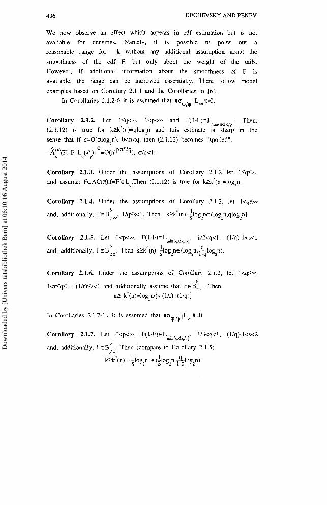
We now observe an effect which appears in cdf estimation but is not

available for densities. Namely, it is possible to point out a

reasonable range for k without any additional assumption about the

smoothness of the cdf F, but only about the weight of the tails.

However, if additional information about the smoothness of F is

available, the range can be narrowed essentially. There follow model

examples based on Corollary 2.1.1 and the Corollaries in [6].

In Corollaries 2.1.2-6 it is assumed that /lo ILoo~~>O. cp3V

Corollary 2.1.2. Let 15q<w, O<p<- and Then,

(2.1.12) is true for k2k'(n)=qlog2n and this estimate is sharp in the

sense that if k=O(olog2n), O<o<q, then (2.1.12) becomes "spoiled":

II~;(F)-F I L (2 ) liP=~(n-poi2q), ~ / q < l . 4 P

Corollary 2.1.3. Under the assun~ptions of Corollary 2.1.2 let I<q+,

and assume: FE AC(IR),~=F'E L .Then (2.1.12) is true for k2k'(n)=log2n. 4

Corollary 2.1.4. Under the assumptions of Corollary 2.1.2, let I<q+ . S 1 and, additionally, FE B l /qP<l . Then k ~ k * ( n ) - ~ l o ~ , n s (lo~n,qlog9n]. P"'

Corollary 2.1.5. Let O<p<m, F ( ~ - F ) E L ~ ~ ~ , ~ , ~ , ~ ,",, 1/2<q<l, ( l / q ) - l a d . S 1 and, additionally, FE B . Then k2k*(n)=Slog2ne (logp,&log2n). PP

Corollary 2.1.6. Under the assumptions of Corollary 2.1.2, let l<q<m, . S

1<6q<m, (l/r)<s<l and additionally assume that F E B , ~ Then,

k> k*(n)=log2ni[s-(1/r)+( 1iq)]

In Corollaries 2.1.7-1 1 it is assumed that \\oV,,, 1 LdI=O.

Corollary 2.1.7. Let O<p<m, F ( ~ - F ) E L , ~ ~ ~ ( ~ ~ ~ , ~ lp,, 1/3<q<l, (l/q)- 1 <s<2 . S

and, additionally, FE B Then (compare to Corollary 2.1.5) PP'

1 1 k>k*(n) E (210g2n ,~ log n) ' I 2

Dow

nloa

ded

by [

Uni

vers

itäts

bibl

ioth

ek B

ern]

at 0

6:10

16

Aug

ust 2

014


Corollary 2.1.8. Under the assumptions of Corollary 2.1.6, assume that . S

FEAC(R) with f=F'€Brm. Then k2k'(n)=l0g~n/[s+l-(l/r)+(l/~)].

Corollary 2.1.9. Under the assumptions of Corollary 2.1.8, assume that . 1

FE AC([R) with f=F'e W , I <p<m, Then k2k8(n)=log2n/[2-(I /r)+(l/q)]. P

Corollary 2.1.10. Under the assumptions of Corollary 2.1.2, let

I<dq<m, ( I l r ) i s i l . I sF~BVr. Then, k2k*(n)4og2n/[s+(llq)].

Corollary 2.1.11. Let O<p<m, F(l-F)€Lmin( (i.e. q=l) and

assume FE AC(R) with density ~=F'E BV,. Then k>k*(n)=(1J2)log2n.

In all Corollaries 2.1.3-11 the estimates about k*(n) are sharp in the

respective sense (compare with Corollary 2.1.2).

Remark 2.1.1. Let us note the computational difficulties which arise if

k is taken much bigger than in the ranges prescribed. The problem is

that, with unbalanced rise of k, cpk, and w become &like functions k~

and both the relative and the absolute computation errors in a 2-k-

neighborhood of any XE[R increase dramatically with k increasing.

2.2. Density Estimation - +M

Let f be a density. Consider Ak(f)(x)= <f,lykj>cpkj(x) with jz."

both cp and y satisfying (2.1.2) and (2.1.3) (note that (2.1.3) can be

loosened to be only satisfied almost everywhere). Under these

assumptions, Ak is known to be shape- preserving ( [ 6 ] ) : Ak(Q is a density. To estimate f using a sample of n observations, we derive an

empirical version of the shape- preserving approximator Ak(f). Let n

A 1 tn(x) be the empirical density fn(x)=f i16(x-~i) , XER, where 6 is the

i= l

delta- function. The shape- preserving density- estimator is

~ ~ ) ( f ) ( x ) = ~ ~ ( ? ~ ( x ) . xe R. (2.2.1)

Remark 2.2.1. The definition (2.2.1) is inspired by [9]. We note that

Dow

nloa

ded

by [

Uni

vers

itäts

bibl

ioth

ek B

ern]

at 0

6:10

16

Aug

ust 2

014


there are several differences between (2.2.1) and the class of

estimators considered in [9]. The estimator i?(f)(x) is shape-

preserving. Further, the function cp may be different from v in 2.2.1.

The functions cp and w are not necessarily such that Ak(f) is an

orthogonal wavelet expansion (although there are admissible cp,yr for

which Ak(f) is an orthogonal expansion).

Remark 2.2.2. Ak(f) is a modification of the operator defined in [I].

We note a major difference: cp and v may be diverse which gives Ak

additional advantages in a number of situations. For example, the

eventual diversity of cp and allows to determine (see 161) the most

general conditions under which the approximation order can be improved.

Besides, it allows a more precise specification of the conditions for

shape- preserving and the differences in this aspect between the case

of cdf and the one of densities. +W n

1 Lemma 2.2.l.(cf. also 191). It holds iL(f)(r)= 1 [,lvk,(~l)]'P,,(x).

J=-W 1=1

We next write analogously to (2.1.9), using ~ i r ) ( f ) = A ~ ( f ) :

11A;j(n-f1 L 4 (P p ) I I P ~ ~ ( ~ , ~ . ~ ) { I I ~ ~ " ' ( D - E A : " ) ( Q 1 L 4 (P p ) I I P + I I A ~ ( Q - ~ L ~ I I P J

(2.2.2)

The bias term having been evaluated in [6], our concern here is to

evaluate the stochastic term IIAF(Q-EA:')(Q 1 L (2 )lip. q P

Theorem 2.2.1. Let f be a density, k ~ w , Oq+. Then:

A) If O<p12, p=min{2,q}, then

Dow

nloa

ded

by [

Uni

vers

itäts

bibl

ioth

ek B

ern]

at 0

6:10

16

Aug

ust 2

014


max (2,p}<q<m, or if q=m and f is continuous, or if Oiq<max{2,p} +m I

min(q/z,q1pJd 1 and sup [ I (J f(x+at)da) x <m.

O l t $h -m 0

Now (2.2.2) can be evaluated by using the above theorem and

Theorem 2.2.1 in [6]. We obtain the following result.

Corollary 2.2.1. Let O<p<m, O<qlm, k€[N. Then

where the term II~:.)(Q-EA:.)(Q ( L (m )ilP is bounded from above by the 4 P

corresponding expression in Theorem 2.2.1, p= , the

term IIAk(f)-flL 11 is bounded from above by the expression given in 9

i)/ii) in Corollary 2.1.1, with F replaced by f.

Remark 2.2.3. Let us mention that in the case p=q=2 (which is most

frequently used in the applications), all requirements on the tail of f

Dow

nloa

ded

by [

Uni

vers

itäts

bibl

ioth

ek B

ern]

at 0

6:10

16

Aug

ust 2

014


that keep the stochastic term at the right-hand side of the estimate of

I I ~ F ( D - ~ ( L (I ) I IP not to explode, are automatically satisfied! At the 9 P

same time, for other values of p and q, if the tail of f is such that f

does not satisfy the conditions (3.27) below, the risk, if measured in

L (I )- norm, might explode. Note also that Kerkyacharian and Picard in 9 P

[9] also put some requirements on the density. It can be seen that

their "Condition Nu implies that f~ L,nin(p ,2,1, n Lmax(p ,Z,I, which

coincides with our condition about the tail behaviour in the partial

case p=q considered there.

Now we shall use Corollary 2.2.1 together with ([6] , Theorem

2.2.1) to obtain estimates of the size of the risk under a variety of

additional conditions on f. For each such set of conditions we shall

be able to find the optimal level of resolution k for which the

wavelet estimator displays best performance. The idea is the

traditional one: since the stochastic term increases, and the bias term

decreases, with the increase of k, the optimal value of k would be the

one for which the order of both terms is the same. This has been also

applied in [9]. Let us note some advantages of our results

(Corollaries 2.2.2- 1 1):

- the results are about shape- preserving estimators;

- the tensor quasi-norms L (2 ) in which the risk is measured are, q P

in our opinion, better suited to reveal the role of the weight of the

tail of the density versus its smoothness;

- the quasi-Banach case O<q<l is included in view of its equal

importance in the applications;

- our results are in terms of the homogeneous analogs of the

inhomogeneous spaces which appear in [9] and, as such, are more

precise, since the bounds from above for our estimates are more

precise. Moreover, this fact makes it possible to improve the results

of the above authors by sometimes imposing weaker assumptions on the

tail of the density. Besides the homogeneous Besov and Triebel-

Lizorkin spaces, the estimates in terms of the functional moduli yield

a variety of estimates in terms of other spaces.

In all corollaries to follow f is a density. In Corollaries

2.2.2-6 110 I L_II>O is assumed. Denote llA:(f)-f 1 L (2 ) ll=&"**. (P,W q P Psi

Dow

nloa

ded

by [

Uni

vers

itäts

bibl

ioth

ek B

ern]

at 0

6:10

16

Aug

ust 2

014

SHAPE-PRESERVING WAVELET ESTIMATORS 44 1

Corollary 2.2.2. Let O<p<m, Ilq<m, O<p<m. Let

f€BV &- q mlnl l , q / 2 . q / p ) k = x 1 l,q12) . Then, the optimal ratio between k

and n is attained for k*(n)=log2n/[1+(2/q)] and -p/lq[l+(2/q)l I

(Pk*)p=0(n P A

1

Corollary 2.2.3. Let O<p<m, l<q<m, fE c:n Lmin{ ~ , q / , q / p , n ~ ~ ~ { 1.~121'

n,k* p iPI3 Then, k*(n)=(log2n)13 , (E ) = ( ). P.4

Corollary 2.2.4. Let O<p<m, I <qlm, O<s<l , S

fEBqm@min( i4n,llnLmu, I , ~ I ~ ] . Then * ( -pW+2~,),

k*(n)=(logB)/(l+2s) and (E"'.* p.q )P=O n (2.2.3)

Corollary 2.2.5. Let O<p<m, (1/2)<q<l, (l/q)-1 <s<l,

f ~ ~ ~ ~ & - ~ ~ ~ ~ ~ ~ , ~ ~ ~ , $ ~ . Then (2.2.3) still holds true.

Corollary 2.2.6. Let O<p<m, 1<&q<m, O<s< I,

" 'L$min{ I , q / ~ , q / p l ~ m u i 1 a12 I . Then p ~ s - ~ l l r ~ + ~ l l ~ ~ l

log2n , (E;:j~=O(i I + Z S ' - ( ~ I I ) + ( ~ I ~ ~ ) +2s-(2/r)+(2i4) (2.2.4)

In Corollaries 2.2.7-1 1 we assume that Ila IL,ll=O. (P-v

Corollary 2.2.7. (compare to Corollary 2.2.5) Let O<p<m, 1/3<q<1, . S

(l/q)-l<s<2, ~ E B ~ ~ & - ~ ~ ~ ~ ~ ~ ~ , ~ ~ ~ , $ , . Then (2.2.3) still holds true.

Corollary 2.2.8. (compare to Corollary 2.2.6). Let O<p<m, l<r<q<m,

O<s<2, fE 'L*mini I , q ~ , q / p l n ~ m t w . { 1,412 1 . Then (2.2.4) continues to

hold true.

Corollary 2.2.9. Let O<p<m, l<&qlm> f~ w2$ r mm( .q/2,q/p)nLmax( 1 .q/2 1

log n ~ 1 2 - ( l l r ) + ( l l q ) l

. Then 2 ,(E;:;*)~=O(n 5 - ( 2 W + ( 2 1 ~ ' ) '9+(2/q)

Dow

nloa

ded

by [

Uni

vers

itäts

bibl

ioth

ek B

ern]

at 0

6:10

16

Aug

ust 2

014


Corollary 2.2.10. Let O<p<m, O<&q<=, O<s5 1,

Corollary 2.2.11, Let O<p<l, q=l, feLmin( lR,llp, nL,Mc(W, f ) ~ BV,.

Then k*(n)=(log2n)/5 . ( P . ~ * ) P = O ( ~ ~ ~ I ~ ) . PSI

Remark 2.2.4. Note the coincidence of the results in Corollaries 2.2.4

and 2.2.7 with the results in 191. Note that Corollaries 2.2.4 and

2.2.7 achieve the same results under weaker assumptions than in the

above paper. In order to clarify this, let q=p in Corollary 2.2.4 or

2.2.7. Then, the coinciding bound for the risk is achieved, according

to 191, for ~ E B : & ~ ~ $ , = B ' & ~ L (where we have used that, for P PI2

l$plm, O<s : B' =BS& ). At the same time, Corollary 2.2.4 or 2.2.7 pM P P

yields the same bound for f ~ ~ ; & m , n ( l , p / 2 , & , n ~ ( 1 , P , 2 1 = Jj;..$p12,?Ll~ This is a demonstration of the effect mentioned that considering

homogeneous, rather than inhomogeneous Besov (or Triebel- Lizorkin)

spaces, brings about a better assessment of the role of the density's

tail weight.

2.3. Asymptotic Normality

There exist (see [ l l ] ) achievable information bounds in the

asymptotic minimax sense for estimators of the cdf. To demonstrate the

asymptotically optimal performance of our wavelet estimators of the

cdf, we have to show that these can achieve the bounds discussed.

We are able to prove asymptotic optimality of A:"'(F) with respect

to the "generalized Cramer- von Mises loss" (the "classical" being the +-

one for q=2): g{[nq12 I 1 A:"'(F)(X)-~(r) 1 qd~(~) ] l lq} , where g(S)= ( 6 I ', ... ~ E R , O<qlp<m . This choice of g corresponds naturally to the quasi-

Dow

nloa

ded

by [

Uni

vers

itäts

bibl

ioth

ek B

ern]

at 0

6:10

16

Aug

ust 2

014


norms in which our evaluations of the risk have been derived. Note

that the function g so selected is an admissible function in the sense

of Millar ([I 11, pp. 162-163) since:

i) g is increasing on [O,w) ; m

ii) there exists a sequence IgnJn, ,, gn- uniformly continuous,

mini 1 51 ,v ) ' , l<p<m

gnfg. Take, for example: g$)= p=l ,

vP' 'min(151,v} , O<p<1

Consider the set C of all continuous cdf on R. Recall the

definition of the set Q from the preliminary section. Denote R c = { o ~ Q :

o(t)52, t~ [O,w)). In the notations of the preliminaries, it is easy to

observe that FE C implies W,E

n

Theorem 2.3.1. Let O<qQ<w. Denote Fn(dx,dx ?... dxJ = l ~ ( d x , ) , xi€ R,

i= 1 A

and let Fn be the empirical distribution function. For w€Rc denote

C W = { F ~ C: ~ ~ ( F , t ) ~ l ~ ( t ) , t~ [O,m)). Then, for every WE Qc and for every

choice of k=k(n) such that 2-k(n)=o(~-1(n-1'2)) as n-, it holds:

Remark 2.3.1. The above theorem indeed shows the asymptotic minimax

optimality of a:"' since it is known for the empirical distribution A

function Fn(x) (see [ l l j ) that it achieves the asymptotic information

bound. Note that for every F E C there exists WEQ such that FE CW (take,

for example, o=wF).

Dow

nloa

ded

by [

Uni

vers

itäts

bibl

ioth

ek B

ern]

at 0

6:10

16

Aug

ust 2

014


As far as the asymptotic rates of convergence in density

estimation are concerned, we shall consider here in detail only the

case when the shape- preserving wavelet estimator is orthogonal.

However, we note that in the general case, the shape- preserving

+M

wavelet is still almost orthogonal: J ~ y ( x ) ~ p ( ~ ) d x r O may only happen .w

[2a]+l, 2aP H if p , ~ : 1 p-v 1 <T) , = , Therefore the basic idea of the

2a , a€ H

proof for the orthogonal case can be carried out in the general non-

orthogonal case, too, with respective modifications.

Theorem 2.3.2. Let lip+, O<Me=, nEN, and suppose that A'"' defined k(n) '

in (2.2.1) is an orthogonal wavelet estimator, with v=(P. Then, for

every s~ (O, l ] , if o SO, and for every s~(O,2], if O ~ . ~ = O , there %'I'

exists a constant c=c(p,s,M)>O such that:

-spl(l+2s) inf s up I I A'" ( o f 1 2 (L )itp>c.n

i ( n ) llfll <M, fTO,llflL,Il=l k ( N P P k ( n ) P,?

Remark 2.3.2 Examples of operators Ak(f) which give admissible A(n) k ( n j

for Theorem 2.3.2, are Ak(Q with ~ ( x ) = (P(x)= ( l l a ) . ~ l-,,,d,, (x-xo), where xo€[-a/2,a/2]. These orthogonal operators are admissible both in

our sense and in the sense of [9].

3. PROOFS OF THE MAIN RESULTS - - - --

Proof of Lemma 2.1.1. The scalar product <F,v > can be transformed k j

as follows: +- +m

W 2 <F,w k .j 2= 2 J ~ ( t ) ~ ( ~ ~ t - j ) d t = 2-V2 J F(I*(T+~))~(T)~T .m .m

+-

=2-W2[1- I ~ ( 2 ~ t - j ) d ~ ( t ) ] -w

Dow

nloa

ded

by [

Uni

vers

itäts

bibl

ioth

ek B

ern]

at 0

6:10

16

Aug

ust 2

014


Here we applied integration by parts and changed the variables. If we

substitute the empirical distribution function instead of F in the

expression obtained and substitute this empirical scalar product in the

formula for Ak(F), we obtain (2.1.7).

Proof of Lemma 2.1.2. We use the fact that Ak(F) is shape- preserving,

as shown in Lemma 2.1.1 of 161. The representation A;)(F)(~)=A~(BJX)

gives then the result.

Proof of Theorem 2.1.1. The following well-known result (see [3]) will

be used as an important technical tool in our evaluations:

If Y,,Y 2,. . . , Yn are i.i.d. random variables , 1 Yi lSA<m, EYi=O,

~ ? = E Y : then:

i) For O<p<2:

El 1yilP6 np12d

1=I

ii) For 2<p<m there exists a constant A >O such that: P

i= l

Other well-known inequalities we shall use are:

maxi l,2P-'].(llf 1 L 11% llg I L 11') for O<p<m, f, g s LP( I ) (3.3) P P

m a x { l . 2 " A " ) ( ~ ~ f l ~ I + I I ~ ~ L I I ) for O<p+. f, p € L P ( ~ ) . (3.4) P P

Now using remark 2.1.1 we observe that the equality n n

i= I 1=1

holds, where for fixed x the i.i.d. random variables

Y ~ = ~ , , F x - E A ~ , ~ F = A F - E X (3.5)

have a finite variance 02(x) and satisfy the conditions I Yl 122, EYi=O

Dow

nloa

ded

by [

Uni

vers

itäts

bibl

ioth

ek B

ern]

at 0

6:10

16

Aug

ust 2

014

446 DECHEVSKYANDPENEV

so that the results (3.1)/(3.2) can be applied.

Denote for a fixed x: B (x)=(E 1 ;\F'(F)(x)- E;\;)(F)(X) 1 p)'lp, P

i=1,2 ,.., n. Applying (3.1)/(3.2) we get

B (x)<n-"*a(x) for O q 1 2 ; P (3.6)

We can continue Inequality (3.7) further to obtain:

In order to be able to further specify (3.6) and (3.8) in terms of

the functions F,cp and v we have to estimate o(x) from above using these

functions. First we shall show that the equality

( k) holds where A are given by

YV ( k ) .k

A =2 {F(x)(I-F(x))+ YV

[v(r)~(r+v-p)(~(2-k((rtv))-~(x))d~} (3.10)

-a

Let us note that in (3.10) (which actually does not depend on x),

the expression F(x)(l-F(x)) for a fixed x has been added and subtracted

in order to better reveal the role of the modulus of smoothness of F.

Dow

nloa

ded

by [

Uni

vers

itäts

bibl

ioth

ek B

ern]

at 0

6:10

16

Aug

ust 2

014


From (3.9) one can see that for any fixed x the non-zero summands

involved in the computation of o2(x) are amongst those for which both k k k conditions 2kx-a< p< 2 x+a and 2 x-a< v< 2 x+a hold simultaneously. But

for those values of p and v the arguments 2 - k ( ~ + ~ ) , 2 - k ( ~ + v ) , ~ ( - a , a ) and x are within a distance less than 21-ka and the summands in (3.10)

can be easily evaluated from above by the corresponding modulus of

smoothness.

We shall indicate the main steps in the proof of (3.9). First,

observe that +m +-

Based on (2.1.7) (see also the proof of Lemma 2.1.1) we could give the

name "empirical scalar products" to the quantities: n

C F : ~ k~ >:=2"(1-A [ Y ( ~ ~ x x ) ) . (3.12)

i= l

Apparently one has: +w +-

~[f$p)(x)l*= I 1 E(<F~V~~><F:W~~>)~~(X).CP~~(X) (3.13) p=-, v=-ca

Combining (3.12) and (3.13), we get:

where the empirical scalar product is taken for n=l. Denote by T a

random variable with the cdf F. Having in mind the definition (3.12),

we obtain easily that:

After some easy application of Integration- by parts and Change- of

variables technique, one gets: Dow

nloa

ded

by [

Uni

vers

itäts

bibl

ioth

ek B

ern]

at 0

6:10

16

Aug

ust 2

014


Combining (3.16) and (3.17) yields then:

a

Utilizing the equality ~ ( z ) d r = l and adding +2F(x), I and

-a -a a

k ~ ( x ) ~ ~ ( r ) Y ( r + v - p ) d z to the expression in the large brackets above,

-a

one obtains:

Dow

nloa

ded

by [

Uni

vers

itäts

bibl

ioth

ek B

ern]

at 0

6:10

16

Aug

ust 2

014


Adding +F(x)~, one finally obtains:

-a

To see that (3.10) follows from (3.18), it remains to show that a

for every s~ R, the expression G(s)= v ( r ) [ ~ ( ~ + s ) + ~ ( ~ - s ) ] d ~ = l . We see J -a

immediately that ~(o)=[Y(a)~-Y(-a)~]=l . Moreover,

00 m

&(s)=/ly(r)v(~+s)di- ( ) ( - d By changing variables r + s i t in .m

I -00

d the first integral, we get @(s)sO.

Dow

nloa

ded

by [

Uni

vers

itäts

bibl

ioth

ek B

ern]

at 0

6:10

16

Aug

ust 2

014


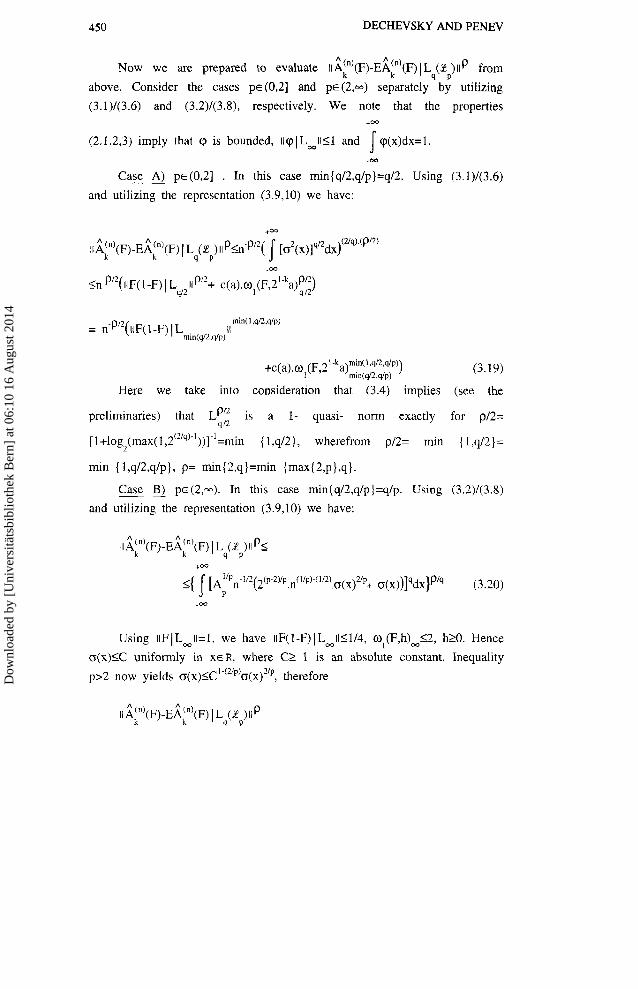
Now we are prepared to evaluate I IA~(F) -E~:" ) (F ) JL (Y )IIP from 4 P

above. Consider the cases pc (0,2] and p~ (2,m) separately by utilizing

(3.1)/(3.6) and (3.2)/(3.8), respectively. We note that the properties + m

(2.1.2,3) imply that cp is bounded, IlcpJLwl151 and cp(x)dx=l. I .m

Case A) p~ (0,2] . In this case min{q/2,q/p}=q/2. Using (3.1)/(3.6) -- and utilizing the representation (3.9,10) we have:

Here we take into consideration that (3.4) implies (see the

preliminaries) that L:;: is a 1- quasi- norm exactly for p/2=

[l+log2(max(1,2~21q)~'))]~1=rnin { 1 ,q/2 1, wherefrom p12= min { I ,q/2 ]=

rnin { 1 ,q/2,q/p], p= min{2,q]=min {max{2,p},q].

Case - B) p~(2 ,m) . In this case min(q/2,q/p]=q/p. Using (3.2)/(3.8)

and utilizing the representation (3.9,10) we have:

Using I IF I L = I I = ~ , we have IIF(1 -F) I Lwll<l/4, ol(F,h)-<2, h2O. Hence

o(x)<C uniforndy in XER, where CT 1 is an absolute constant. Inequality

p>2 now yields o ( x ) 5 ~ ' - ( ~ / ~ ) o ( x ) ~ ~ ~ , therefore Dow

nloa

ded

by [

Uni

vers

itäts

bibl

ioth

ek B

ern]

at 0

6:10

16

Aug

ust 2

014


where p is selected so that LPIp is a 1- quasi- norm, i.e., analogously 4 /P

to case A), plp= min(l,q/p}= min{l,ql2,q/p}, p= min{p,q}=min{max(2,p],q}. Hence,

To finish the proof of Theorem 2.1.1 we need to show that if F is

a cdf and F(x)(l-F(x))€Lh for some h ~ ( 0 , ~ ) then ~ ~ ( F , h ) ~ = o , , ( l ) , h 4

holds. First consider the case llh<m. Clearly FE B V l a V h . Moreover +m +m

( v ~ F ) % VIF holds. From the properties of the integral modulus of -00 . m

smoothness (see 1171, Section 3) we have for h ~ [ l , m ) , h>O: ~ ~ ( F , h ) ~ l

l /h += l/h +m l/h- h ( V ~ F ) " ' ~ h ( V{F)= h - o ( l ) In the case k(O.1) our . m - 00

definition of the integral modulus of smoothness (see the

Preliminaries) is easily seen to be equivalent for p=1 to the

definition given in [18]. Abusing notation, we write +m I

h l lh o , ( ~ , h ) ~ = m a x { sup { J [IlF(x+at)-~(x) 1 da] dx} ,

Olt<h -m

m m x + h x+h

Hence o l (~ ,h )h<{ I 1 V F J dx+ 1 V FI dx)lih for any mE R. For F is .m

X m X

x+h with bounded variation, it is well known that l im V F=O for almost

h-+O+ x

Dow

nloa

ded

by [

Uni

vers

itäts

bibl

ioth

ek B

ern]

at 0

6:10

16

Aug

ust 2

014


every xe[R. Choose m to be e.g. a median of F. Then:

x+h x+h m Note that V F5 min { V F, V F). Utilizing IIF(1-F) lLhll<m, the

x -m x convergence of W , ( F , ~ ) ~ --4 can be obtained using Lebesgue's dominated

h 4 0 +

convergence theorem. Hence the case h ~ ( 0 , l ) is also proved. Finally

let us note that for q=w: 11F(l-F)IL~ll<l14, i.e. F(l-F)€LW and in this

case, if F is continuous then w,(~,2"~a)~=o,(l),k-. Theorem 2.1.1

is proved.

Note about the proofs of the corollaries. The proofs are obtained by a

straightforward equalizing of the convergence rates of the stochastic

and bias term under the assumptions of the respective corollary for the

bias in [6].

Proof of Lemma 2.2.1, Replacing the scalar products <f,v > by the kj

n

1 empirical scalar products <f:v >= - lyrkj(xi) immediately yields the kj n

i= 1

result.

Proof of Theorem 2.2.1. The main steps in the proof follow the steps

in the proof of Theorem 2.1.1. We shall use of the Inequalities (3.6)

and (3.8). To be able to further specify them in terms of the

functions f,cp and v , we have to estimate o(x) from above using these

functions. Following the steps in the proof of Theorem 2.1.1 we get

the representation

( k) but now with A being equal to

+- PV +m +-

Dow

nloa

ded

by [

Uni

vers

itäts

bibl

ioth

ek B

ern]

at 0

6:10

16

Aug

ust 2

014


This is the analog of (3.10) in the case of densities.

Since y satisfies both (2.1.2) and (2.1.3) now. we know that 00

d x ) M , 11 y 1 LwIIS1 and J y(x)dx=l hold. Utilizing these properties and .w

the fact that ykp and ykv have not fully overlapping supports for p#v,

we can claim that:

0 < 2 - ~ J ykv(t)f(t)dts Jy(2*t-v)f(t)dtSl . Hence -00 .'=-

Dow

nloa

ded

by [

Uni

vers

itäts

bibl

ioth

ek B

ern]

at 0

6:10

16

Aug

ust 2

014


there are only a finite number of non-zero summands involved in the

calculation of 02(x) in (3.22). These are such that 2kx-a<y<2k+a and

2kx-a<v<2kx+a should simultaneously hold. But for those values of p and

v the arguments x and 2-k(.r+p),2'k(z+v), TE(-a,a) are at a distance

less than 21'ka and the summands in M'~'(x) can be easily bounded from

above by the corresponding modulus of smoothness of f. Then

substitution from (3.24) into (3.22) yields

where I(x)= max li (x) 1, J(x)= max l j (x) 1 can be evaluated by the p , v CL,V P

corresponding moduli of smoothness.

Now we are prepared to evaluate ili:'(f)-~;\:"'(f) 1 L (2 ) i P from 4 P

above. Consider the cases p ~ ( 0 , 2 ] and p ~ ( 2 , m ) separately by utilizing

(3.1)/(3.6) and (3.2)/(3.8), respectively.

Case A) p ~ ( 0 , 2 ] . In this case min(q/2,q/p]=q/2. Using - - (3.1)/(3.6), utilizing the representation (3.22, 23) and the inequality

for 02(x), we have, invoking (3.4) analogous to the proof of (3.19): +m

I I ~ ~ ) ( ~ ) - E ~ : ~ ) ( ~ ) I L 4 (P P ) iP<n-Pn( I [ d ( ~ ) ] ~ ' ~ d n ) ' s " ~ ~ ~ '

for p=min{2,q]. Case A) of the theorem's assertion now follows by

utilizing the fact that f€L1 and, by Holder's inequality,if f e L n L , 1 2

O<s <s Sw, then f~ L , sl<s<s2. 1 2 7

Case B) p~(2 ,m) . In this case min{q/2,q/p}=q/p. Using (3.2)/(3.8) - - and utilizing the representation (3.22,23), the inequality for 02(x)

Dow

nloa

ded

by [

Uni

vers

itäts

bibl

ioth

ek B

ern]

at 0

6:10

16

Aug

ust 2

014


and the inequality (Zlx, 11 xi la, O<a<l, for a = l / p and a=l/2. we

i I

have:

Analogously to (3.25) we use (3.4) and for p=min{ l ,q] , can

continue the evaluation from above in (3.26) to obtain:

Now the assertion of the theorem in Case B) follows easily by the

same arguments as in Case A).

Now we have to find conditions on the density f e L X that force the

Dow

nloa

ded

by [

Uni

vers

itäts

bibl

ioth

ek B

ern]

at 0

6:10

16

Aug

ust 2

014


corresponding smoothness moduli ~ ~ ( f , h ) ~ in (3.25,26) to tend to zero

when h a + . The case l < k m is considered for example in [12] and it

states that c 0 ~ ( f , h ) ~ 4 , h a + always when f€Lh. For hc(0,1), it is not

difficult to prove (based on Lebesgue's dominated convergence theorem)

that the condition { f€Lh, ~ , ( f ,h )~=o , , ( l ) , h 4 } is equivalent to 1

man{ sup [ /(I1 f(x+at) ( da)'dx]lm, llf (Lhli I<-. Therefore, in our context O<tlh --. 0

we have to require that f f L l belongs also to L for O<p<2, and to q12

L q P for 2<p<m, or, equivalently, '

fE Lmin( I . q ~ Z , ~ / ~ ) @ r n ~ ~ ( I . q / ~ ) w I

for O<p<m. and sup [ / (/I f(x+at) 1 da)"1i11(q12,q1P' dx]- for qsmax {2,p 1. 0 s t 6h

-m o -

Note that, in view of max{ l,q/2]21, the generalized Minkowski

inequality implies 00 1

This is equivalent to impose the following requirement on the

density f: {f: EL and mm(q/*,q/p.l )+maxi 1 .q/>)

Theorem 2.2.1 is proved.

Proof of Theorem 2.3.1. Fix WEQ, The space 2 (L )P is, as mentioned in P q

the preliminaries, a complete quasi-normed abelian group which is

1 metrizable. It is a metric space exactly when 7 max{l, I l + L - l } P S ' P 9

(note that (l/p)5(l/q)). For this choice of p* we have:

Dow

nloa

ded

by [

Uni

vers

itäts

bibl

ioth

ek B

ern]

at 0

6:10

16

Aug

ust 2

014


Now COcC implies +=

.-a A

Since we know that Fn is asymptotically optimal, it suffices to

prove that +m

A (n) A Substituting Ak (F)(x) and F,(X) in (3.28) we obtain:

+-a n

+QJ

where Yi(x)= 1 [ 1 - ~ ( 2 ~ ~ . - j ) - @ ( x - ~ ~ ) ] ~ ( 2 ~ x - j) ,i= 1,2,..,n, XE R, @(.)

j=-w

being the Heaviside's function. (Note that Yi also depend on k but

this dependence has been suppressed in the notation). For a fixed

value of x the random variables Yi(x) are i.i.d., with expected value

EY.(x)=Ak(F)(x)-F(x). This is exactly the quantity which has been

evaluated from above in [6] (see also Corollary 2.1.1). Using this

evaluation and the generalized Minkowski's Inequality, we have:

with some positive constant c. Denote the first and second summands in

Dow

nloa

ded

by [

Uni

vers

itäts

bibl

ioth

ek B

ern]

at 0

6:10

16

Aug

ust 2

014


(3.29) by I and J, respectively.

Utilizing 0~(~.2~~~a)~62o,(~,2~~~a)~, we have, by definition of Cw

and by the choice of k=k(n),

Here we used that l i m o(h)=O,i.e., o and on formally commute. h+O+

To evaluate the expression I from above, we use again the Inequalities

(3.1) and (3.2) (let us note that for a fixed x: Yi(x)-EYi(x) are

i.i.d. zero- mean random variables and that I Yi(x)-EYi(x) 152 holds).

Put &x)=E(Y,(x))*. Like in the proof of Theorem 2.1.1 we can write:

p=-m V=-- Denoting by T a random variable with a cdf F, the following

( k) evaluation of the term 6 can be given:

PV

.m .M

After integrating by parts and changing variables, we have easily:

with a similar expression for v replacing p. In order to apply Cauchy-Schwarz Inequality to evaluate from above

the expression E[(~-Y(~~T-~)-~(X-T))(~-Y(~~T-V)-B(X-T))],W~ need an

estimate for [E 1 I -Y(~~T-~) -B(x-T) 1 2 ] 1 1 2 . Again after integration by

Dow

nloa

ded

by [

Uni

vers

itäts

bibl

ioth

ek B

ern]

at 0

6:10

16

Aug

ust 2

014


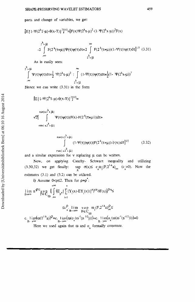
parts and change of variables, we get:

k 2 x-p QJ

-2 1 ~ ( 2 - ~ ( r + p ) ) ~ ( r ) ~ ( r ) d r + 2 I ~(2-~(r+p))(l-~(r))ly(r)dr]"~ (3.31) -00 k

2 x-p As is easily seen:

k 2 x-p 00

1 1 I Y(r)yr(~)d)dr=~ Y(2*x-p12 ; j' (I-Y(r))~(r)dr=$l- Y(~*x-p))' -00 k

2 x-p Hence we can write (3.31) in the form

k mu(-a ,Z x-pJ

and a similar expression for v replacing p can be written.

Now, on applying Cauchy- Schwarz inequality and utilizing

(3.30,32) we get finally: sup o(x)< ~ ~ o ~ ( F , 2 ' - ~ a ) ~ (cdO). Now the X

estimates (3.1) and (3.2) can be utilized.

i) Assume O<p<2. Then for P = ~ * : +m n

<cp. 1 im s u p w,(~,2 '-~a)L1 a n - w FE C,

..

c. 1 i m(o(2 l.ka))P=c. 1 i m(o(on(o-I (n-ll2))))=c. 1 i m(~~(w(w"(n'"~))))=~ n+m n+m n+-

Here we used again that w and on formally commute.

Dow

nloa

ded

by [

Uni

vers

itäts

bibl

ioth

ek B

ern]

at 0

6:10

16

Aug

ust 2

014


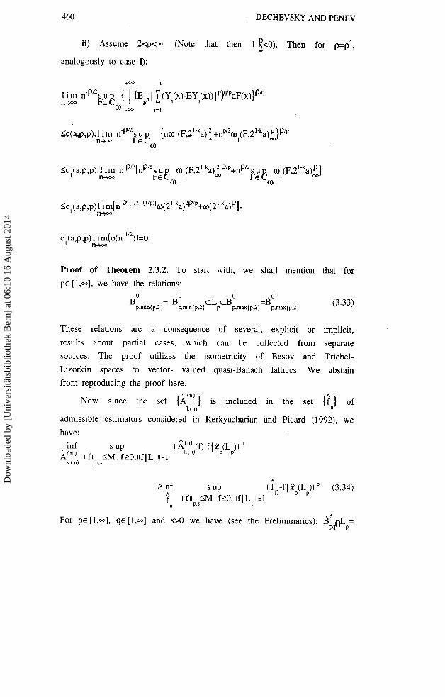
ii) Assume 2<p<m. (Note that then 1-&o). Then for p p * ,

analogously to case i):

Proof of Theorem 2.3.2. To start with, we shall mention that for

p~ [ l , ~ ] , we have the relations:

B0 0

CL do 0

= B =B p.minlp.21 p,minIp,21 P p.maxlp.2) p,maxlp,Z)

(3.33)

These relations are a consequence of several, explicit or implicit,

results about partial cases, which can be collected from separate

sources. The proof utilizes the isometricity of Besov and Triebel-

Lizorkin spaces to vector- valued quasi-Banach lattices. We abstain

from reproducing the proof here.

Now since the set is included k(n)

admissible estimators considered in Kerkyacharian

have:

in the set {fn} of

and Picard (1992), we

. . ^f llfll 5M. RO,llf~L1lI=1 n PS

For p ~ [ l , w ] , q ~ [ l , m ] and s>O we have (see the Preliminaries): BS nL = W P

Dow

nloa

ded

by [

Uni

vers

itäts

bibl

ioth

ek B

ern]

at 0

6:10

16

Aug

ust 2

014

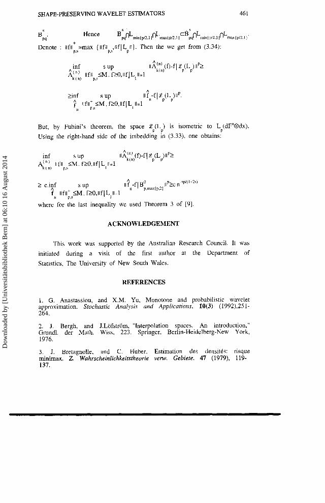
SHAPE-PRESERVING WAVELET ESTIMATORS 46 1

But, by Fubini's theorem, the space 2 (L ) is isometric to L (dFnOdx). P P P

Using the right-hand side of the imbedding in (3.33), one obtains:

where for the last inequality we used Theorem 3 of [9].

ACKNOWLEDGEMENT

This work was supported by the Australian Research Council. It was

initiated during a visit of the first author at the Department of

Statistics, The University of New South Wales.

REFERENCES

1. G. Anastassiou, and X.M. Yu, Monotone and probabilistic wavelet approximation. Stochastic Analysis and Applications, lO(3) (1992),25 1 - 264.

2. J. Bergh, and J.Lofstrom, "Interpolation spaces. An introduction," Grundl. der Math. Wiss, 223. Springer, Berlin-Heidelberg-New York, 1976.

3. J. Bretagnolle, and C. Huber. Estimation des densitis: risque minimax. 2. Wahrscheinlichkeitstheorie vem. Gebiete. 47 (1979), 119- 137.

Dow

nloa

ded

by [

Uni

vers

itäts

bibl

ioth

ek B

ern]

at 0

6:10

16

Aug

ust 2

014

462 DECHEVSKYANDPENEV

4. C.K. Chui, "An Introduction to Wavelets," Academic Press, Boston, 1992.

5. I. Daubechies, "Ten Lectures on Wavelets," SIAM, Philadelphia, 1992.

6. L.T. Dechevsky, and S.I. Penev, On shape- preserving probabilistic wavelet approximators. To appear in Stochastic analysis and applications, 15(2) (1997).

7. M. Frazier, B. Jawert and G.Weiss," Littlewood- Paley theory and the study of function spaces," AMS, Providence,R.I., 1991.

8. H. Johnen, and K.Scherer, On the equivalence of the K-functional and moduli of continuity and some applications, In "Constructive theory of functions of several variables, Oberwolfach'76," (W. Schempp, and K. Zeller, Eds), Lect. Notes in Math. 571, pp. 119-140, Springer, Berlin Heidelberg New York, 1977.

9. G. Kerkyacharian, and D. Picard, hensity estimation in Besov spaces. Statistics& Probability letters, 13 (1992), 15-24.

10. Y. Meyer, "Ondelettes et opkrateurs I," Hemann, Paris, 1990.

11. P. W. Millar, The minimax principle in asymptotic statistical theory. In "Ecole d'EtC de Probabilitts de Saint-Flour XI-1981," (P. Hennequin, Ed), Lect. Notes in Math. 976, pp. 75-265, Springer, Berlin Heidelberg New York, 1983.

12. S. M. Nikol'skii, "Approximation of functions of several variables and imbedding theorems," Springer, Berlin New York, 1975.

13. J. Peetre, "New thoughts on Besov spaces," Duke University Math. Series, Durham, 1976.

14. J. Peetre, and G. Sparr, Interpolation of normed abelian groups, Ann. Math. Pura Appl. 92 (1972), 217- 262.

15. P. Petrushev, and V.A. Popov, "Rational approximation of real functions," Cambridge University Press, Cambridge, 1987.

16. B. Sendov, and V.A. Popov, "Averaged moduli of smoothness," Bulgarian Academy of Sciences, Sofia, 1983.

17. A. F. Timan, "Theory of approximation of functions of a real variable," Hindustan Publ. Corp., Delhi, 1966.

18. H. Triebel, "Theory of function spaces," Monographs in Mathematics, Vol. 78, Birkhauser, Basel, 1983.

Dow

nloa

ded

by [

Uni

vers

itäts

bibl

ioth

ek B

ern]

at 0

6:10

16

Aug

ust 2

014

on shape-preserving wavelet estimators of cumulative distribution functions and densities

Documents