on neumann type problems for non-local equations …
TRANSCRIPT
ON NEUMANN TYPE PROBLEMS FOR NON-LOCAL
EQUATIONS SET IN A HALF SPACE
GUY BARLES, EMMANUEL CHASSEIGNE, CHRISTINE GEORGELIN,AND ESPEN R. JAKOBSEN
Abstract. We study Neumann type boundary value problems for nonlocalequations related to Levy processes. Since these equations are nonlocal, Neu-
mann type problems can be obtained in many ways, depending on the kind of
“reflection” we impose on the outside jumps. To focus on the new phenom-enas and ideas, we consider different models of reflection and rather general
non-symmetric Levy measures, but only simple linear equations in half-space
domains. We derive the Neumann/reflection problems through a truncationprocedure on the Levy measure, and then we develop a viscosity solution the-
ory which includes comparison, existence, and some regularity results. For
problems involving fractional Laplacian type operators like e.g. (−∆)α/2,we prove that solutions of all our nonlocal Neumann problems converge as
α→ 2− to the solution of a classical Neumann problem. The reflection mod-els we consider include cases where the underlying Levy processes are reflected,
projected, and/or censored upon exiting the domain.
1. Introduction
In the classical probabilistic approach to elliptic and parabolic partial differ-ential equations via Feynman-Kac formulas, it is well-known that Neumann typeboundary conditions are associated to stochastic processes having a reflection onthe boundary. We refer the reader to the book of Freidlin [9] for an introductionand to Lions and Sznitman [17] for general results. A key result in this directionis roughly speaking the following: for a PDE with Neumann or oblique boundaryconditions, there is a unique underlying reflection process, and any consistent ap-proximation will converge to it in the limit (see [17] and Barles & Lions [5]). Atleast in the case of normal reflections, this result is strongly connected to the studyof the Skorohod problem and relies on the underlying stochastic processes beingcontinuous.
The starting point of this article was to address the same question, but nowfor jump diffusion processes related to partial integro-differential equations (PIDEsin short). What is a reflection for such processes, and is a PIDE with Neumannboundary conditions naturally connected to a reflection process? It turns out thatthe situation is more complicated in this setting, at least the questions have to bereformulated in a slightly different way. In this article we address these questions
2000 Mathematics Subject Classification. 35R09 (45K05), 35B51, 35D40 .Key words and phrases. Nonlocal equations, Neumann boundary conditions, jumps, Levy mea-
sure, reflection, viscosity solutions.Jakobsen was supported by the Research Council of Norway through the project “Integro-
PDEs: Numerical methods, Analysis, and Applications to Finance”.
1
2 BARLES, CHASSEIGNE, GEORGELIN, AND JAKOBSEN
through an analytical PIDE approach where we keep in mind the idea of having areflection process but without defining it precisely or even proving its existence.
For jump processes which are discontinuous and may exit a domain withouttouching its boundary, it turns out that there are many ways to define a “reflec-tion” or a “process with a reflection”. This remains true even if we restrict ourselvesto a mechanism which is connected to a Neumann boundary condition (see below).But because of the way the PIDE and the process are related, defining a reflectionon the boundary will change the equation inside the domain. This is a new nonlocalphenomenon which is not encountered in the case of continuous processes and PDEs.
PIDE with Neumann-type boundary condition – In order to simplify thepresentation of paper and focus on the main new ideas and phenomenas, we considerdifferent models of reflections and rather general non-symmetric Levy measures, butonly for problems involving linear equations set in simple domains. The cases wewill consider already have interesting features and difficulties. To be precise, weconsider half space domains Ω :=
(x1, . . . , xN ) = (x′, xN ) ∈ RN : xN > 0
and
simple linear Neumann type problems that we write asu(x)− I[u](x)− f(x) = 0 in Ω,
− ∂u∂xN
= 0 in ∂Ω,(1.1)
or sometimes as F (x, u, I[u]) = 0 in Ω,
− ∂u∂xN
= 0 in ∂Ω,
where F (x, r, l) = r − l − f(x) and
I[u](x) = limb→0+
∫b<|z|
[u(x+ η(x, z))− u(x)] dµ(z).
We will assume that f ∈ Cb(Ω), i.e. f is bounded and continuous, that µ is anonnegative Radon measure satisfying∫
|z|2 ∧ 1 dµ(z) <∞,(1.2)
and that
x+ η(x, z) ∈ Ω for all x ∈ Ω , η(x, z) = z if x+ z ∈ Ω.(1.3)
Note that I[u] is a principal value (P.V.) integral, and that (1.2) is the mostgeneral integrability assumption satisfied by the Levy measure associated to anyLevy process [1]. When η(x, z) ≡ z, then I[u] is the generator of a stochasticprocess which can jump from x ∈ Ω to x + z with a certain probability, see e.g.[1, 8, 10]. Assumption (1.3) is a type of reflection condition preventing the jump-process from leaving the domain: nothing happens and η(x, z) = z if x + z ∈ Ω,while if x + z /∈ Ω, then a ”reflection” is performed in order to move the particleback to a point P (x, z) = x+ η(x, z) inside Ω. Note that we have to check at somepoint that the reflection is consistent with a Neumann boundary condition.
NEUMANN PROBLEMS 3
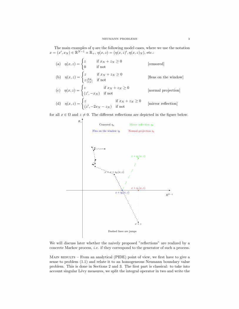
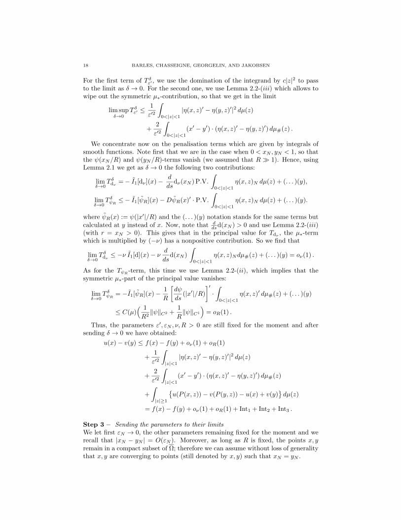
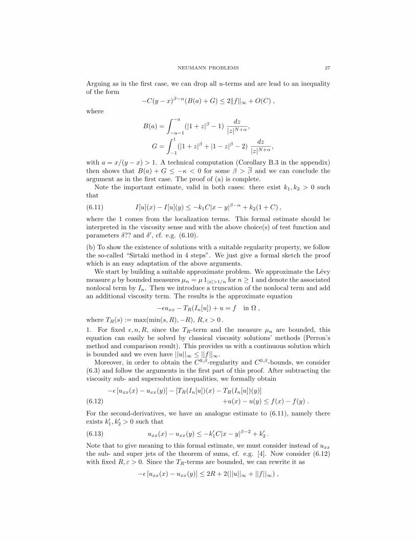
The main examples of η are the following model cases, where we use the notationx = (x′, xN ) ∈ RN−1 × R+, η(x, z) = (η(x, z)′, η(x, z)N ), etc.:
(a) η(x, z) =
z if xN + zN ≥ 0
0 if not[censored]
(b) η(x, z) =
z if xN + zN ≥ 0
z xN|zN | if not
[fleas on the window]
(c) η(x, z) =
z if xN + zN ≥ 0
(z′,−xN ) if not[normal projection]
(d) η(x, z) =
z if xN + zN ≥ 0
(z′,−2xN − zN ) if not[mirror reflection]
for all x ∈ Ω and z 6= 0. The different reflections are depicted in the figure below.
x = x+ ηa(x, z)
x+ z
Censored ηa
x+ ηb(x, z)
Flea on the window ηb
x+ ηc(x, z)
Normal projection ηc
x+ ηd(x, z)
Mirror reflection ηd
Dashed lines are jumps
RN−1
R+
We will discuss later whether the naively proposed ”reflections” are realized by aconcrete Markov process, i.e. if they correspond to the generator of such a process.
Main results – From an analytical (PIDE) point of view, we first have to give asense to problem (1.1) and relate it to an homogeneous Neumann boundary valueproblem. This is done in Sections 2 and 3. The first part is classical: to take intoaccount singular Levy measures, we split the integral operator in two and write the
4 BARLES, CHASSEIGNE, GEORGELIN, AND JAKOBSEN
equation in a more convenient way. Here classical arguments in viscosity solutiontheory are used, see e.g. [4] and references therein. Viscosity solution theory is alsoused to give a good definition of the Neumann boundary conditions.
If µ is a nice bounded measure, then the problem (1.1) can be solved easily with-out caring much about the Neumann boundary condition. Moreover, the solutionswill be uniformly bounded by ||f ||∞. Intuitively (1.1) carries the information thatthe particles remain in Ω since they can only jump inside Ω. This mass conservationis an other way to understand that we are dealing with a (homogeneous) Neumanntype of boundary condition.
When µ then is a singular measure, we can approximate it by a sequence ofbounded measures (µn)n, consider the associated (uniformly bounded!) solutions(un)n, and wonder what the limiting problem is if µn converges to µ in a suitablesense. This is the way we choose to make sense of both the definition of problem(1.1) and the associated notion of (viscosity) solutions. We point out here that the“real” Neumann boundary condition arises only if the measure is singular enough.In the other cases, either the process will never reach the boundary as in thecensored case for α-stable process with α < 1 (see e.g. [6]), or the equation willhold up to the boundary.
The natural next step is then to prove uniqueness results for all the above modelsand equations. In this paper different types of proofs are given depending on thesingularity of the measure and the structure of the “reflection” mechanism at theboundary. These results are given in Sections 4 – 6. The first case we treat iswhen the jump function η enjoys a contraction property in the normal direction.This covers all the non-censored cases listed above – models (b)–(d). Had we had acontraction in all directions, then the usual viscosity solution doubling of variablesargument would work. Here we have to modify that argument to take into accountthe special role of the normal direction.
The second case we consider is the censored case (a) when the singularity of themeasure is not too strong. By this we mean typically a stable process with Levymeasure with density dµ
dz ∼1
|z|N+α for α ∈ (0, 1). We construct an approximate
subsolution which blows up at the boundary and this allows us to derive a compar-ison result by a penalization procedure. Such a construction is related to the factthat the process does not reach the boundary in this case, see e.g. [6].
The last case is the censored case (a) when the singularity is strong, i.e. whenα ∈ [1, 2). This case requires much more work because no blow-up subsolutions ex-ist here. In fact, when α ∈ [1, 2), the censored process does reach the boundary (seee.g. [6]). We first prove that the Neumann boundary condition is already encodedin the equation under the additional assumption that the solution is β-Holder con-tinuous at the boundary for some β > α−1. Then we prove a comparison result forsub/super solutions with this Holder regularity at the boundary. The proof is thensimilar to the proof in the α < 1 case, except that the special subsolutions in thiscase are bounded and only penalize the boundary when the sub/super solutions areHolder continuous there. Finally, we construct solutions in this class. In dimen-sion N = 1, we use and prove that any bounded uniformly continuous solution isHolder continuous provided µ satisfies some additional integrability condition. Inhigher dimensions, we use and prove a similar result under additional regularityassumptions on f in the tangential directions.
NEUMANN PROBLEMS 5
Finally, in Section 7 we show that all the proposed nonlocal models converge tothe same local Neumann problem when the Levy measure approches the “local” case
α = 2. More precisely, we consider Levy measures µα with densities (2−α) g(z)|z|N+α ,
where g is a nonnegative bounded function which is C1 in a neighborhood of 0 andsatisfies g(0) > 0. In this case we prove that whatever nonlocal Neumann modelwe use, the solutions uα converge as α → 2 to the unique viscosity solution of thesame limit problem, namely
(1.4)
−a∆u− b ·Du+ u = f in Ω ,∂u
∂n= 0 in ∂Ω ,
where a := g(0) |SN−1|N and b := Dg(0) |S
N−1|N .
Related work – One of the first papers on the subject was Menaldi and Robin[15]. In that paper stochastic differential equations for reflection problems aresolved in the case of diffusion processes with inside jumps, i.e. when there are nojumps outside the domain. They use the method of “penalization on the domain”inspired by Lions, Menaldi and Sznitman [18].
In model (a) (the censored case), any outside jump of the underlying processis cancelled (censored) and the process is restarted (resurrected) at the origin ofthat jump. We refer to e.g. [6, 10, 13, 16] for more details on such processes. Theprocess can be constructed using the Ikeda-Nagasawa-Watanabe piecing togetherprocedure [6, 10, 16], as Hunt processes associated to some Dirichlet forms [6, 13],or via the Feynman-Kac transform involving the killing measure [6]. In particular,the underlying processes in this paper are related to the censored stable processesof Bogdan et al. [6] and the reflected α-stable process of Guan and Ma [13]. Butnote that we essentially only construct the generators and not yet the processesthemselves. On the technical side, we use viscosity solution methods, while [6, 13]use the theory of Dirichlet forms and potential theory. Our assumptions are alsodifferent, e.g. with our arguments we treat more general measures and we have thepotential to treat non-linear problems, while [6, 13] e.g. treat much more generaldomains.
Let us also mention that the ”natural” Neumann boundary condition for thereflected α-stable process of Guan and Ma [13] is slighly different from the onewe consider here. They claim that the boundary condition arising through thevariational formulation and Green type of formulas is
limt→0
t2−α∂u
∂xN(x+ teN ) = 0.
This formula allows the normal derivative ∂u∂xN
to explode less rapidly than |xN |α−2.
In model (b) outside jumps are stopped where the jump path hits the boundary,and then the process is restarted there. Model (c) is close to the approach of Lions-Sznitman in [17], and here outside jumps are immediately projected to the boundaryalong the normal direction. This type of models will be thoroughly investigated inthe forthcoming paper [3] by three of the authors, but this time in the setting of fullynon-linear equations set in general domains. Note that model (b) and (c) coincidein one dimension, i.e. when N = 1. Finally, in model (d), outside jumps are mirrorreflected at the boundary. This is intuitively the natural way of understanding a
6 BARLES, CHASSEIGNE, GEORGELIN, AND JAKOBSEN
”reflection”, but the model may be problematic to handle in general domains dueto the possibility of multiple reflections. E.g. it is not clear to us if it correspondto an underlying Markov process in a general domain.
To the best of our knowledge, processes with generators of the form (b)–(d) havenot been considered before. E.g. the works of Stroock [19] and Taira [20, 21] seemnot to cover our cases because their integrodifferential operators involve measuresand jump vectors η that are more regular than ours. Moreover in these works, it isthe measure and not η that prevents the process to jump outside Ω.
In the case of symmetric α-stable processes (a subordinated Brownian motion),our formulation follows after a “reflection” on the boundary. So such processescan be constructed from a Brownian motion by first subordinating the processand then reflecting it. Another possible way to construct a “reflected” process inthis case would be to reflect the Brownian motion first and then subordinate thereflected process. A related approach is described e.g. in Hsu [14] where pure jumpprocesses like Levy processes are connected via the Dirichlet-Neumann operatorto the trace at the boundary of a Reflected Brownian Motion in one extra spacedimension Ω × R+. An analytic PIDE version of this approach is introduced byCaffarelli and Silvestre in [7] in order to obtain Harnack inequalities for solutions ofintegrodifferential equations, and then these ideas have been used by many authorssince.
Finally we mention the more classical work of Garroni and Menaldi [11], where alarge class of uniformly elliptic integro differential equations are considered. Thereare two main differences with our work: (i) In [11] the principle part of all equationsis a local non-degenerate 2nd order term. This allows the non-local terms to becontrolled by local terms (the solution and its 1st and 2nd derivatives) via interpo-lation inequalities, and the local W 2,p and C2,α theories can therefore be extendedto this nonlocal case. In our paper, it is the non-local terms that are the principalterms, and interpolation is not available. In addition, most of our results can beextended to degenerate problems. (ii) In [11] Dirichlet type problems are consid-ered, and the authors have to assume extra decay properties of the jump vector ηnear the boundary, conditions that are not satisfied in our Neumann models.
2. Assumptions and Definition of solutions
In this section we state the assumptions on the problem (1.1) that we will usein the rest of the paper, give the definition of solutions for (1.1), and show that thequantities in this defintion is well-defined under our assumptions.
In this paper we let Du(x) and D2u(x) denote the gradient and hessian matrixof a function u at x. We also define P (x, z) = x + η(x, z), and then we can stateour assumptions as follows:
(Hf ) f ∈ Cb(Ω).
(Hµ) The measure µ is the sum of two nonnegative Radon measures µ∗ and µ#,
µ = cµ∗ + µ#,
where c is either 0 or 1, µ∗ is a symmetric measure satisfying (1.2) and∫|z|<1
|z| dµ∗ =∞, and
∫RN
(1 ∧ |z|) dµ# <∞.

NEUMANN PROBLEMS 7
(H0η) Neuman problem: P (x, z)N = xN + η(x, z)N > 0 for any x, z and
η(x, z) = z for any xN + zN > 0.
(H1η) At most linear growth of the jumps: there exists cη > 0 such that
|η(x, z)| ≤ cη|z| for any x, z.
(H2η) Antisymmetry with respect to the z′-variables: for any i = 1, . . . , (N − 1),
η(x, σiz)i = −η(x, z)i where σiz = (z1, . . . ,−zi, . . . , zN ) .
(H3η) Weak continuity condition:
η(y, z)→ η(x, z) µ-a.e. as y → x.
(H4η) Continuity in the x′-variable:
|η(x′, s, z)′ − η(y′, s, z)′| ≤ C|z||x′ − y′| for any x′, y′, z and any s > 0.
(H5η) Non-censored cases: Contraction in the N -th direction:
|P (x, z)N − P (y, z)N | ≤ |xN − yN |.(H6
η) Censored case: For all z 6= 0 and x ∈ Ω,
η(x, z) =
z if xN + zN ≥ 0,
0 otherwise.
Remark 2.1. Assumption (Hµ) means that we can decompose µ into a sum of a sin-gular symmetric Levy measure and a not so singular Levy measure. Symmetric heremeans that
∫RN χ(z) dµ = 0 for any odd µ-integrable function χ. This assumption
covers the stable, the tempered stable, and the larger class of self-decomposableprocesses in RN , cf. chapter 1.2 in [1]. In all these cases the Levy measures satisfy
dµ
dz=
g(z)
|z|N+αfor α ∈ (0, 2),
and (Hµ) holds with c = 0 if α ∈ (0, 1), while if α ∈ [1, 2) and g is Lipschitz inB1(0) and bounded, then (Hµ) holds with c = 1. In the last case we may take
dµ∗dz
=h(z)
|z|N+αand
dµ#
dz=g(z)− h(z)
|z|N+αfor h(z) := min
|y|=|z|g(y),
and note that h is symmetric and g − h is nonnegative. More generally, we canconsider measures where dµ
dz = g(z)dµ∗dz and µ∗ is symmetric.
Remark 2.2. The cases (a), (b), (c), and (d) mentioned in the introduction satisfyassumptions (Hi
η) for i = 0, 1, 2, 3, 4, where in fact (H4η) holds with C = 0. Assump-
tion (H5η) holds except in case (a), and case (a) is equivalent to (H6
η). Note that ηis continuous in x for z 6= 0 in (b), (c), and (d), while in (a), η is continuous excepton the codimension 1 hypersurface zN = xN.
Now we will define generalized solutions in the viscosity sense, and to do thatwe need the following notation:
I[φ] = Iδ[φ] + Iδ[φ] ,
where
Iδ[φ] =
∫|z|≥δ
φ(x+ η(x, z))− φ(x) dµ(z) .

8 BARLES, CHASSEIGNE, GEORGELIN, AND JAKOBSEN
The Iδ-term is well-defined for any bounded function φ. For the Iδ-term there aretwo cases, depending on whether c = 0 or 1 in (Hµ). If c = 0, a Taylor expansionshows that Iδ[φ](x) is well-defined for φ ∈ C1 and x ∈ Ω. If c = 1, and the measureµ is very singular, we add and subtract a compensator and write
Iδ[φ](x) = Iδ[φ](x) + P.V.
∫|z|<δ
Dφ(x) · η(x, z) dµ(z),
for
Iδ[φ](x) :=
∫|z|<δ
φ(x+ η(x, z))− φ(x)−Dφ(x) · η(x, z) dµ(z).
By the C2-regularity of φ, these two terms will be well-defined – see Lemma 2.1below. Note that this results is non-trivial because the compensator is not welldefined in general!
Definition 2.1. Assume that (Hµ), (Hiη) for i = 0, 1, 2 hold.
(i) A bounded usc function u is a viscosity subsolution to (1.1) if, for any test-function φ ∈ C2(RN ) and maximum point x of u− φ in B(x, cηδ) ∩ Ω,
F (x, u(x), Iδ[φ] + Iδ[u]) ≤ 0 if x ∈ Ω and
either F (x, u(x), Iδ[φ] + Iδ[u]) ≤ 0 if x ∈ ∂Ω and c = 0,
or − ∂φ
∂xN(x) ≤ 0 if x ∈ ∂Ω and c = 1.
(ii) A bounded lsc function v is a viscosity supersolution to (1.1) if, for any test-function φ ∈ C2(RN ) and minimum point x of v − φ in B(x, cηδ) ∩ Ω,
F (x, v(x), Iδ[φ] + Iδ[v]) ≥ 0 if x ∈ Ω and
either F (x, v(x), Iδ[φ] + Iδ[v]) ≥ 0 if x ∈ ∂Ω and c = 0,
or − ∂φ
∂xN(x) ≥ 0 if x ∈ ∂Ω and c = 1.
(iii) A viscosity solution is both a sub- and a supersolution.
Remark 2.3. The constant cη is defined in (H1η). If u and φ are smooth and x is a
maximum point of u− φ over B(x, cηδ) ∩ Ω, then by (H1η),
u(x)− φ(x) ≥ u(x+ η(x, z))− φ(x+ η(x, z)) for all |z| < δ.
If we rewrite this inequality and integrate, we find formally that Iδ[u](x) ≤ Iδ[φ](x).Lemma 2.1 below makes this computation rigorous. From this inequality it is easyto prove that classical (sub)solutions of (1.1) are viscosity (sub)solutions. Moreover,smooth viscosity (sub)solutions are classical (sub)solutions (simply take φ = u).
Remark 2.4. In general to pose boundary value problems in the viscosity sense,one requires that either the minimum of the equation and the boundary conditionis nonpositive or the maximum of the equation and the boundary condition isnonnegative. Here this is not the case and for a natural reason. If the measure isvery singular (and c = 1) then the equation cannot hold on the boundary and theinequality holds just for the boundary condition. In the c = 0 case, on the contrary,the equation will hold up to the boundary and the boundary condition can not beimposed in general. In other words, we only end up with a Neumann boundarycondition if c = 1, i.e. the measure has a “strong” singular part µ∗. In this case

NEUMANN PROBLEMS 9
the intensity of small jumps is so strong that the jump-reflection mechanisms, e.g.as in (a) – (d), are not enough to prevent the process from “diffusing” onto theboundary, and we need to add a reflection process at the boundary to keep theprocess inside (just as in the case of Brownian motion). We also note that thesymmetry of µ∗ is a natural condition in order to obtain Neumann and not obliquederivative boundary conditions, cf. Lemma 3.3 and proof.
We now prove that Iδ[φ] is well-defined for φ ∈ C2.
Lemma 2.1. Assume (Hµ) and (Hiη) for i = 0, 1, 2, and let x ∈ Ω, φ ∈ C2, and
δ > 0. Then Iδ[φ](x) is well-defined since
Iδ[φ](x) = Iδ[φ](x) + P.V.
∫|z|<δ
Dφ(x) · η(x, z) dµ(z),
and the compensator term satisfies
P.V.
∫|z|<δ
Dφ(x) · η(x, z) dµ(z)
=
∫|z|<δ
Dφ(x) · η(x, z) dµ#(z) + c
∫xN<|z|<δ
Dφ(x) · η(x, z) dµ∗(z).
Moreover, there is R = R(x, η) > 0 such that
Iδ[φ](x) = oδ(1)‖φ‖C2(BR(x)) as δ → 0.
In the following, we often drop the P.V. notation for such integrals since theymay be expressed in terms of converging integrals. Note that the integral overxN < |z| < δ need not vanish since this regions exceeds the boundary and henceη(x, z) will not be odd there.
To prove Lemma 2.1, we need the following result.
Lemma 2.2. Assume (Hµ) and (Hiη) for i = 0, 1, 2, and let xN > 0, ρ ∈ (0, xN ),
and v ∈ RN be a fixed vector.
(i) For r ∈ (0, ρ),∫r<|z|<ρ v · η(x, z) dµ(z) =
∫r<|z|<ρ v · η(x, z) dµ#(z), and
P.V.
∫|z|<ρ
v · η(x, z) dµ(z) =
∫|z|<ρ
v · η(x, z) dµ#(z) .
(ii) For r ∈ (0, 1),∫r<|z|<δ v
′ · η(x, z)′ dµ(z) =∫r<|z|<δ v
′ · η(x, z)′ dµ#(z), and
P.V.
∫|z|<δ
v′ · η(x, z)′ dµ(z) =
∫|z|<δ
v′ · η(x, z)′ dµ#(z) ,
(iii) For r ∈ (0, 1),∫r<|z|<δ
η(x, z)N dµ∗(z) ≥∫r<|z|<δzN>xN
(zN − xN ) dµ∗(z) ≥ 0 .
Proof. (i) If |z| < ρ < xN , then η(x, z) = z by (H0η). Hence η is odd with respect
to the z variable, and the integral with respect to the symmetric part cµ∗ is zero.Passing to the limit as r → 0 and using the integrability of µ# along with (H1
η)finishes the proof of (i).
10 BARLES, CHASSEIGNE, GEORGELIN, AND JAKOBSEN
(ii) Let σ be the rotation σ(z′, zN ) = (−z′, zN ). Since µ∗ is symmetric,∫r<|z|<δ
v′ · η(x, σz)′ dµ∗(z) =
∫r<|z|<δ
v′ · η(x, z)′ dµ∗(z).
Other hand, since η(x,−z′, zN )′ = −η(x, z′, zN )′ by (H2η), the above integral is zero.
The result on the principal value is obtained as in the first case, after letting r → 0.(iii) Let us decompose∫
r<|z|<δη(x, z)N dµ∗(z) =
∫r<|z|<δ
−xN≤zN≤xN
η(x, z)N dµ∗(z)
+
∫r<|z|<δzN>xN
η(x, z)N dµ∗(z) +
∫r<|z|<δzN<−xN
η(x, z)N dµ∗(z) .
The integral over −xN ≤ zN ≤ xN vanishes since η(y, z) = z in this region and µ∗is symmetric. By (H0
η) we have that η(x, z)N ≥ −xN if zN < −xN and η(x, z) =zN > xN if zN > xN . Hence by symmetry of µ∗,∫
r<|z|<δη(x, z)N dµ∗(z) ≥
∫r<|z|<δzN>xN
(zN − xN ) dµ∗(z) ≥ 0,
and the proof is complete.
Proof of Lemma 2.1. The expression for Iδ is obtained by adding and substractingthe compensator term. The first integral in this expression is well-defined sincethe integrand is smooth and bounded by the function 1
2 |z|2 maxB(x,R) |D2φ|, for
R = maxy∈B(0,δ) |η(x, y)|, which is an µ-integrable function over B(0, δ). Moreover,∫0<|z|<δ |z|
2 dµ(z) = oδ(1) as δ → 0 since |z|2 is µ-integrable near 0.
In the compensator term, the integral with respect to µ# exists by (H1η), while
the integral with respect to µ∗ over B(0, xN ) vanishes by Lemma 2.2-(i). Since |z|is integrable near the origin for µ#, this term is |Dφ(x)|oδ(1) as δ → 0.
3. Derivation of the boundary value problem - PIDE approach
In this section we derive the boundary value problems from approximate prob-lems involving a sequence of bounded positive Radon measures µk = 1|z|>1/kµconverging to µ. Assume (Hµ) and let µk# = 1|z|>1/kµ# and µk∗ = 1|z|>1/kµ∗,it then easily follows that
(H1µ) lim
k→+∞
∫|z| ∧ 1 dµk#(z) =
∫|z| ∧ 1 dµ#(z),
(H2µ) lim
k→+∞
∫|z|2 ∧ 1 dµk∗(z) =
∫|z|2 ∧ 1 dµ∗(z),
(H3µ) lim
k→+∞
∫|z| ∧ 1 dµk∗(z) =∞.
The approximation problem we consider is then given by
u(x)− Iµk [u](x) = f(x) in Ω,(3.1)
where, for φ ∈ Cb(Ω),
Iµk [φ](x) =
∫|z|>0
φ(x+ η(x, z))− φ(x) dµk(z).
NEUMANN PROBLEMS 11
Since the measures µk are bounded, this equation holds in a classical, pointwisesense. Moreover, it is well-posed in Cb(Ω) and the solutions uk are uniformlybounded in k:
Lemma 3.1. Assume (Hf ), (Hµ), (H0η), and (H3
η).
(a) For every k, there is a unique pointwise solution uk of (3.1) in Cb(Ω).(b) If uk and vk are pointwise sub- and supersolutions of (3.1), then uk ≤ vk in Ω.(c) If uk is a pointwise solution of (3.1), then ‖uk‖L∞(Ω) ≤ ‖f‖L∞(Ω).
Proof. (a) Let T : Cb(Ω)→ Cb(Ω) be the operator defined by
Tu := u− ε(u− Iµk [u]− f
),
where ε < (1 + 2‖µk‖1)−1 and ‖µk‖1 is the total (finite!) mass of the measure µk.Then T is a contraction in the Banach space Cb(Ω) since
‖Tu− Tv‖∞ ≤ (1− ε)‖u− v‖∞ + 2ε‖µk‖1‖u− v‖∞≤(1− ε(1 + 2‖µk‖1)
)‖u− v‖∞
≤ C(k)‖u− v‖∞ ,
and C(k) < 1. Hence there exists a unique uk ∈ Cb(Ω) such that Tuk = uk, whichis equivalent to (3.1).
(b) If supΩ(u − v) is attained at a point x ∈ Ω, then by the equation and theeasy fact that Iµk [φ] ≤ 0 at a maximum point of φ,
supΩ
(u− v) = u(x)− v(x) ≤ Iµk [u− v](x) ≤ 0.
The general case follows after a standard penalization argument.(c) Follows from (b) since ±‖f‖L∞(Ω) are sub- and supersolutions of (3.1).
The limiting problem can be identified through the half relaxed limit method:
Theorem 3.2. Assume (Hf ), (Hµ), and (Hiη) for i = 0, 1, 2, 3 hold. Then the
half-relaxed limit functions
u(x) = lim supk→+∞,y→x
uk(y) and u(x) = lim infk→+∞,y→x
uk(y)
are respectively sub- and supersolutions of the Neumann boundary problem in thesense of Definition 2.1.
In the proof we will need the following result whose proof is given at the end ofthis section.
Lemma 3.3. Assume (Hiη) holds for i = 0, 1, 2, (Hµ) holds with c = 1, and let
δ > 0 and γµk,r(x) :=∫|z|<r η(x, z) dµk(z). If yk → x ∈ ∂Ω as k →∞, then
|γµk,δ(yk)| → ∞ andγµk,δ(yk)
|γµk,δ(yk)|→ −n,
where n = (0, 0, . . . , 0,−1) is an outward normal vector of ∂Ω.
Proof of Theorem 3.2. Since the proofs are similar for u and u, we only do the onefor u. Let δ > 0 and φ ∈ C2, and assume that u − φ has a maximum point x inB(x, cηδ) ∩ Ω. Let us first consider the case when x ∈ Ω, i.e. when xN > 0. Bymodifying the test-function, we may always assume that the maximum is strict.
12 BARLES, CHASSEIGNE, GEORGELIN, AND JAKOBSEN
By standard arguments, uk − φ has a maximum point yk in B(x, cηδ), and whenk → +∞,
yk → x and uk(yk)→ u(x).
Let δk = δ − |x− yk| and 0 < r ≤ δk, and note that B(yk, cηr) ⊂ B(x, cηδ). Sincethe max of (uk − φ) in B(yk, cηr) is attained at yk, we find that
(Iµk)r[uk](yk) :=
∫|z|<r
uk(yk + η(yk, z))− uk(yk) dµk
≤∫|z|<r
φ(yk + η(yk, z))− φ(yk) dµk = (Iµk)r[φ](yk).
Hence, since uk is a pointwise solution of (3.1), we find for all 0 < r ≤ δk,
uk(yk)− (Iµk)r[φ](yk)− (Iµk)r[uk](yk) ≤ f(yk),
where (Iµk)r[uk](x) :=∫|z|≥r uk(x+ η(x, z))− uk(x) dµk(z).
We want to pass to the limit in this equation and consider first the (Iµk)r-term.By the definition of u and (H3
η),
lim supk→+∞
uk(yk + η(yk, z)) ≤ u(x+ η(x, z)) for a.e. z.
Hence, since we integrate away from the singularity of µ, we can use Fatou’s lemmaand (H1
µ) and (H2µ) to show that
lim supk→∞
(Iµk)r[uk](yk) ≤∫|z|>r
u(x+ η(x, z))− u(x) dµ(z) = Ir[u](x).
To pass to the limit in the (Iµk)r-term, we have to write it as
(Iµk)r[φ](yk) =∫|z|<r
φ(x+ η(yk, z))− φ(yk)−Dφ(yk) · η(yk, z) dµk(z)︸ ︷︷ ︸
=(Iµk )r[φ](yk)
+γµk,r(yk) ·Dφ(yk),
where γµk,r(x) :=∫|z|<r η(x, z) dµk(z). For |z| < r, a Taylor expansion then yields∣∣φ(yk + η(yk, z))− φ(yk)−Dφ(yk) · η(yk, z)
∣∣ ≤ ‖D2φ‖L∞(B(x,cηr))|z|2.
Hence by (H1η), (H3
η), (H1µ) and (H2
µ), we can use the Dominated ConvergenceTheorem to show that
(Iµk)r[φ](yk)→∫|z|<r
φ(x+ η(x, z))− φ(x)− η(x, z)Dφ(x) dµ(z) = Ir[φ](x).
Next, by Lemma 2.1,
γµk,r(yk) =
∫|z|<r
η(yk, z) dµk#(z) + c
∫yk,N≤|z|<r
η(yk, z) dµk∗(z),
where the last integral is understood to be zero if yk,N > r. Note that sinceyk,N → xN > 0, the domain of integration of the µ∗-integral is always bounded
away from z = 0 when k is big. Along with (H3η) and (H2
µ), this allows us to pass to
NEUMANN PROBLEMS 13
the limit in the µ∗-integral using the Dominated Convergence Theorem. Similarly,we may pass to the limit in the µ#-integral by (H1
η), (H3η) and (H1
µ). We find that
γµk,r(yk,N )→ γr(x) :=
∫|z|<r
z dµ#(x) + c
∫xN≤|z|<r
η(x, z) dµ∗(x)
= P.V.
∫|z|<r
η(x, z) dµ(x) =: γr(x),
where we used Lemma 2.1 again. Hence we can conclude that
limk→∞
(Iµk)r[φ](yk) = Ir[φ](yk) + γr(x) ·Dφ(x) = Ir[φ](x).
Since δk → δ, we end up with the following limit equation,
u(x)− Ir[φ](x)− Ir[u](x) ≤ f(x)
for every 0 < r < δ. Using the Dominated Convergence Theorem again, we sendr → δ and obtain the subsolution condition for (1.1) at the point x ∈ Ω.
The second part of the proof is to consider the case of when x ∈ ∂Ω, i.e thecase when xN = 0. We first do it in the case c = 1. By adding, subtracting, anddivinding by terms, we may rewrite the subsolution condition as
uk(yk)− (Iµk)δ[φ](yk)− (Iµk)δ[uk](yk)− f(yk)
|γµk,δ(yk)|− γµk,δ(yk) ·Dφ(yk)
|γµk,δ(yk)|≤ 0.
By Lemma 3.3, |γµk,δ(yk)| → ∞, and since uk and f are uniformly bounded,
uk(yk)
|γµk,δ(yk)|,
f(yk)
|γµk,δ(yk)|,
(Iµk)δ[uk](yk)
|γµk,δ(yk)|,
all converge to zero. The same is true for
(Iµk)δ[φ](yk)
|γµk,δ(yk)|
since the integrand of the numerator is controlled by ‖D2φ‖∞|z|21|z|<δ and µk
satisfies (H1µ). Using Lemma 3.3 again, we have γµk,δ(yk)/|γµk,δ(yk)| → −n, so
that we may go to the limit in the above inquality to find that
− ∂φ
∂xN(x) =
∂φ
∂n(x) ≤ 0 .
In the case when c = 0, the measure µ = µ# which less singular than µ∗. Thesame line of arguments as in the proof for x ∈ Ω (much easier this time) now showsthat the equation holds at x ∈ ∂Ω.
Proof of Lemma 3.3. First note that by Lemma 2.2 with yk instead of x and µk
instead of µ,
γµk,δ(yk)′ =
∫|z|<δ
η(yk, z)′ dµk(z) =
∫|z|<δ
η(yk, z)′ dµk#(z) ,
which remains uniformly bounded in k because of (H1η) and our assumption on µ#.
Since yk,N → xN = 0, we can assume that 0 ≤ yk,N < δ, and by Lemma 2.2,
(γµk,δ)N (yk) =
∫|z|<δ
η(yk, z)N dµk#(z) +
∫yk,N<|z|<δ
η(yk, z)N dµk∗(z) .

14 BARLES, CHASSEIGNE, GEORGELIN, AND JAKOBSEN
As above, the first integral is uniformly bounded as k → ∞. For the second one,we send r → 0 in Lemma 2.2-(iii) to find that
(3.2)
∫|z|<δ
η(yk, z)N dµk∗(z) ≥
∫|z|<δ
yk,N<zN
(zN − yk,N ) dµk∗(z) ≥ 0,
and, since yk,N → 0, we can then use Fatou’s lemma to show that∫|z|<δzN>0
zN dµ∗(z) ≤ lim infk→∞
∫|z|<δ
yk,N<zN
(zN − yk,N ) dµk∗(z) .
Applying symmetry of the measure µ∗ twice, we are lead to∫|z|<δzN>0
zN dµ∗(z) =1
2
∫|z|<δ
|zN | dµ∗(z) =1
2N
∫|z|<δ
N∑i=1
|zi| dµ∗(z),
so by taking (H3µ) into account, there is a constant C = C(N) > 0 such that∫
|z|<δzN>0
zN dµ∗(z) ≥C
2N
∫|z|<δ
|z| dµ∗(z) =∞.
Hence we have proved that (γµk,δ)N (yk) → ∞ as k → ∞, and if we use that(γµk,δ
)′(yk) is uniformly bounded, we see that
γµk,δ(yk)
|γµk,δ(yk)|=( (γµk,δ)
′(yk)
|γµk,δ(yk)|,
(γµk,δ)N (yk)
|γµk,δ(yk)|
)−→ (0, 0, · · · , 0, 1) = −n.
4. Comparison in non-censored cases
In this section we prove a comparison result for the non-censored cases, i.e.under assumption (Hi
η) for i = 0, . . . , 5. These assumptions covers all the examplesgiven in the introduction, except example (a) – the censored case. As a conseqenceof the comparison result and the results of the previous sections, we also obtainwell-posedness for (1.1). The comparison result is the following:
Theorem 4.1. Assume (Hµ), (Hf ), and (Hiη) hold for i = 0, 1, 2, 3, 4, 5. Let u
be a bounded usc subsolution of (1.1) with data f ∈ Cb(RN ), v be a bounded lscsupersolution of (1.1) with data g ∈ Cb(RN ) such that f ≤ g in Ω. Then u ≤ v onΩ.
From this result it follows that the half-relaxed limits in Theorem 3.2 satisfyu ≤ u in Ω. Since the opposite inequality is always satisfied, this means that u :=u = u is solution of (1.1) according to Definition 2.1. Uniqueness and continuousdependence (on f) follows from Theorem 4.1 by standard arguments and we havethe following result:
Corollary 4.2. Under the assumptions of Theorem 4.1, there exits a unique vis-cosity solution of (1.1) depending continuously on f .
Proof of Theorem 4.1. We argue by contradiction assuming that M := supΩ(u −v) > 0. We provide the full details only when c = 1. The case c = 0 is far simplersince the equation then holds even on the boundary.
To get a contradiction, we first introduce the function
ΨR(x) := u(x)− v(x)− ψR(x, x) ,
NEUMANN PROBLEMS 15
where ψR is a localisation term which makes the max attained:
ψR(x, y) = ψ(|xN |/R) + ψ(|yN |/R) + ψ(|x′|/R) + ψ(|y′|/R) ,
with ψ a smooth function such that
ψ(s) =
0 for 0 ≤ s < 1/2 ,
increasing for 1/2 ≤ s < 1 ,
2(‖u‖∞ + ‖v‖∞ + 1) for s ≥ 1 .
Of course, MR := max ΨR → M as R → ∞ so that for R big, max ΨR > 0. Thenthere are two cases for such R > 0:
(a) either there exists a maximum point xR of ΨR which is not located on theboundary. In this case the proof is quite classical: we use the doubling of variablesplus a localisation term around xR by considering the max of
u(x)− v(y)− |x′ − y′|2
ε′2− |xN − yN |
2
ε2N
− ψR(x, y)− σ|x− xR|4 ,
where σ > 0 is small. The localization term σ|x − xR|4 is chosen so that xR isthe unique maximum point of x 7→ ΨR(x) − σ|x − xR|4, and by choosing σ smallenough, the contribution of this function in the integral term is small1.
Hence the maximum points (x, y) of the above test-function converges necessarelyto (xR, xR) as ε′, εN → 0 and they are also bounded away from the boundary ifε′, εN are small enough. This property implies that we can use directly the equationand obtain max ΨR ≤ 0, which is a contradiction.
(b) or any maximum point xR is located on the boundary. In this case we use thedoubling of variables plus some extra term to push the points inside (see below)1:
Φε′,εN ,ν,R(x, y) := u(x)−v(y)−|x′ − y′|2
ε′2−|xN − yN |
2
ε2N
−ψR(x, y)+dν(xN )+dν(yN ) .
In this case we can assume without loss of generality that the maximum points x, yare always such that 0 < xN , yN < 1, whatever εN , ε
′, ν > 0 are.Note that in both cases we take two distinct real parameters ε′, εN > 0 in order
to take into account the special contraction property in the N -th direction, see(H5
η). Now, since case (a) is rather standard, we only provide a proof of case (b)which is more involved.
The term dν plays the role of a distance to the boundary of the domain; suchterm is usual in classical Neumann proofs in order to prevent the maximum pointsto be on the boundary. More precisely, for ν > 0, we take dν(·) = νd(·) where d isa smooth function such that
d(s) =
s for 0 ≤ s < 1/2 ,
increasing for 1/2 ≤ s < 1 ,
1 for s ≥ 1 .
Let us note that if 0 < ν < 1 and R 1 are fixed, then Φ := Φε′,εN ,ν,R ≤ 0for |x|, |y| large enough, while, by choosing x = y in a suitable way by taking intoaccount the fact that M > 0, we have Φε′,εN ,ν,R(x, x) > 0 for ν small; hence the
1In the viscosity inequalities, the various penalization terms are only integrated near the origin,e.g. in |z| < δ. Therefore we do not need to worry about the integrability at infinity of |x|2 and
|x|4 with respect to the measure µ.
16 BARLES, CHASSEIGNE, GEORGELIN, AND JAKOBSEN
maximum of Φ is attained at some point (x, y) ∈ Ω2, that we still denote by (x, y)for simplicity.
After proving that the points x, y are inside Ω, we are going to first let εN → 0,then ε′ → 0, then ν → 0 and finally R→∞. Because of this use of parameters, wehave
MεN ,ε′,ν,R := max ΦεN ,ε′,ν,R →M > 0 .
In particular, this implies that
xN − yN = O(εN ) , x′ − y′ = O(ε′) ,|x′ − y′|2
ε′2= oεN ,ε′(1) ,
where the O(εN ), O(ε′) are uniform with respect to all the parameters, and theoεN ,ε′(1) means precisely that after passing to the limit as εN → 0, we are left witha quantity which is an oε′(1). Also note that
u(x)− v(y) = M + oεN ,ε′,ν,R(1) ,
where the order of the parameters is important as explained above.
Step 1 – Pushing the points inside.We denote by
ϕ(x, y) :=|x′ − y′|2
ε′2+|xN − yN |2
ε2N
+ ψR(x, y)− dν(xN )− dν(yN ) ,
where we have dropped the parameters for the sake of simplicity of notations.In this step, we prove that the F -viscosity inequalities hold for u and v. Accord-
ing to Definition 2.1, this is clearly the case if c = 0 since these viscosity inequalitieshold even if the maximum or minimum points are on the boundary.
In the c = 1 case, let us assume that the maximum point (x, y) is such thatxN = 0, then x is a (global) maximum point of the function z 7→ u(z)−v(y)−ϕ(z, y)
and, thanks to Definition 2.1, we should have − ∂ϕ∂xN
(x, y) ≤ 0. But, recalling that∂ψR∂xN
is zero in a neighborhood of the boundary, we have
− ∂ϕ
∂xN(x, y) = −2(xN − yN )
ε2N
− ∂ψR∂xN
(x, y) +d
dsdν(0) =
2yNε2N
+ ν > 0 ,
which is a contradiction. Therefore xN cannot be zero and a similar argumentshows that yN > 0 as well, hence both x and y are inside Ω.
Step 2 – Writing the viscosity inequalities and sending δ to zero.We introduce a (small) fixed parameter 0 < δ < 1 which is the parameter appearingin Definition 2.1 in order to give sense to different terms in the equation. We writethe definition of viscosity sub and super solutions, using the test-function in theball Bδ for a δ < ρ := min(xN , yN , 1), and the functions u and v outside this ball.Since u is a viscosity subsolution and the function u(·) − v(y) − ϕ(·, y) reaches amaximum at x, then we have the viscosity subsolution condition that we write asfollows, thanks to Lemma 2.1:
u(x)−∫|z|<δ
[ϕ(x+ η(x, z), y)− ϕ(x, y)−Dxϕ(x, y) · η(x, z)] dµ(z)
− P.V.
∫|z|<δ
Dxϕ(x, y)η(x, z) dµ(z)−∫|z|≥δ
[u(x+ η(x, z))− u(x)] dµ(z) ≤ f(x) .

NEUMANN PROBLEMS 17
For simplicity of notations, we leave out the P.V. notation since the integral canbe expressed as converging integrals and we use the notation P (x, z) := x+η(x, z).Next we use Lemma 2.2-(i) and the similar super solution condition on v to get
−∫|z|<δ
[ϕ(P (x, z), y)− ϕ(x, y)−Dxϕ(x, y) · η(x, z)] dµ(z)
−Dxϕ(x, y) ·∫|z|<δ
η(x, z) dµ#(z)
−∫|z|<δ
[ϕ(x, P (y, z))− ϕ(x, y) +Dyϕ(x, y) · η(y, z)] dµ(z)
+Dyϕ(x, y) ·∫|z|<δ
η(y, z) dµ#(z)
−∫|z|≥δ
[u(P (x, z))− v(P (y, z))− u(x) + v(y)] dµ(z)
+ u(x)− v(y) ≤ f(x)− f(y) .
In order to pass to the limit as δ → 0 to get rid of the test-function ϕ, we useLemma 2.1 for all the terms which are smooth functions: the integrals over B(0, δ)all vanish as δ → 0 and we are left with limit of the integral over |z| > δ. Tothis end, we split this integral into two integrals, one over |z| ≥ 1 (which isindependent of δ of course) and the other over δ ≤ |z| < 1 that we have to dealwith.
Using the definition of the maximum point for Φ, we have that for any z:
u(P (x, z))− v(P (y, z))− ϕ(P (x, z), P (y, z)) ≤ u(x)− v(y)− ϕ(x, y) .
Hence, it follows that
u(P (x, z))− v(P (y, z))− (u(x)− v(y))
≤ |P (x, z)N − P (y, z)N |2
ε2N
− |xN − yN |2
ε2N
+|P (x, z)′ − P (y, z)′|2
ε′2− |x
′ − y′|2
ε′2
+ ψR(P (x, z), P (y, z))− ψR(x, y)
− dν(P (x, z)N ) + dν(xN )− dν(P (y, z)N ) + dν(yN ) ,
and we put this inequality into the integral over δ ≤ |z| < 1 which gives rise toseveral terms denoted by (with obvious notation):∫δ≤|z|<1
u(P (x, z))− v(P (y, z))− u(x) + v(y)
dµ(z) ≤ T δεN + T δε′ + T δψR + T δdν .
As for the εN -terms, we get rid of them by (H5η) which implies T δεN ≤ 0. Then for
the ε′-terms we write
T δε′ =
∫δ≤|z|<1
( |P (x, z)′ − P (y, z)′|2
ε′2− |x
′ − y′|2
ε′2
)dµ
≤ 1
ε′2
∫δ≤|z|<1
|η(x, z)′ − η(y, z)′|2 dµ(z)
+2
ε′2
∫δ≤|z|<1
(x′ − y′) · (η(x, z)′ − η(y, z)′) dµ(z) .
18 BARLES, CHASSEIGNE, GEORGELIN, AND JAKOBSEN
For the first term of T δε′ , we use the domination of the integrand by c|z|2 to passto the limit as δ → 0. For the second one, we use Lemma 2.2-(iii) which allows towipe out the symmetric µ∗-contribution, so that we get in the limit
lim supδ→0
T δε′ ≤1
ε′2
∫0<|z|<1
|η(x, z)′ − η(y, z)′|2 dµ(z)
+2
ε′2
∫0<|z|<1
(x′ − y′) · (η(x, z)′ − η(y, z)′) dµ#(z) .
We concentrate now on the penalisation terms which are given by integrals ofsmooth functions. Note first that we are in the case when 0 < xN , yN < 1, so thatthe ψ(xN/R) and ψ(yN/R)-terms vanish (we assumed that R 1). Hence, usingLemma 2.1 we get as δ → 0 the following two contributions:
limδ→0
T δdν =− I1[dν ](x)− d
dsdν(xN ) P.V.
∫0<|z|<1
η(x, z)N dµ(z) + (. . . )(y),
limδ→0
T δψR ≤− I1[ψR](x)−DψR(x)′ · P.V.∫
0<|z|<1
η(x, z)N dµ(z) + (. . . )(y).
where ψR(x) := ψ(|x′|/R) and the (. . . )(y) notation stands for the same terms butcalculated at y instead of x. Now, note that d
dsd(xN ) > 0 and use Lemma 2.2-(iii)(with r = xN > 0). This gives that in the principal value for Tdν , the µ∗-termwhich is multiplied by (−ν) has a nonpositive contribution. So we find that
limδ→0
T δdν ≤ −ν I1[d](x)− ν d
dsd(xN )
∫0<|z|<1
η(x, z)Ndµ#(z) + (. . . )(y) = oν(1) .
As for the TψR -term, this time we use Lemma 2.2-(ii), which implies that thesymmetric µ∗-part of the principal value vanishes:
limδ→0
T δψR = −I1[ψR](x)− 1
R
[dψ
ds(|x′|/R)
]′·∫
0<|z|<1
η(x, z)′ dµ#(z) + (. . . )(y)
≤ C(µ)( 1
R2‖ψ‖C2 +
1
R‖ψ‖C1
)= oR(1) .
Thus, the parameters ε′, εN , ν, R > 0 are still fixed for the moment and aftersending δ → 0 we have obtained:
u(x)− v(y) ≤ f(x)− f(y) + oν(1) + oR(1)
+1
ε′2
∫|z|<1
|η(x, z)′ − η(y, z)′|2 dµ(z)
+2
ε′2
∫|z|<1
(x′ − y′) · (η(x, z)′ − η(y, z)′) dµ#(z)
+
∫|z|≥1
u(P (x, z))− v(P (y, z))− u(x) + v(y)
dµ(z)
= f(x)− f(y) + oν(1) + oR(1) + Int1 + Int2 + Int3 .
Step 3 – Sending the parameters to their limitsWe let first εN → 0, the other parameters remaining fixed for the moment and werecall that |xN − yN | = O(εN ). Moreover, as long as R is fixed, the points x, yremain in a compact subset of Ω; therefore we can assume without loss of generalitythat x, y are converging to points (still denoted by x, y) such that xN = yN .
NEUMANN PROBLEMS 19
Combining (H3η) and (H4
η), we obtain in particular that
limεN→0
|η(x, z)′ − η(y, z)′| ≤ C|z||x′ − y′| for µ-a.e. z .
Then, (H1η) and the integrability condition on µ# justify that we can use dominated
convergence in Int2. The argument is similar for Int1, using the domination
|η(x, z)′ − η(y, z)′|2 ≤ (2cη)2|z|2 .
So we find that limεN→0 Int2 = 0 while
limεN→0
Int1 ≤ C|x′ − y′|2
ε′2
∫|z|<1
|z|2dµ(z) = oε′(1).
The oR(1) and oν(1) terms are uniform with respect to the other parameters, sothere is no problem to send εN , ε
′ → 0 here. Next, since |x− y| → 0 as εN , ε′ → 0
here, we may assume that x, y → x ∈ Ω by considering a subsequence is necessary.By continuity of f , it then follows that
(f(x)− f(y)
)→ 0.
We then pass also to the limit as ν → 0 and get:
(4.1) u(x)− v(x) ≤ lim supν→0
lim supε′→0
lim supεN→0
[Int3] + oR(1) .
Passage to the limit in the Int3 term is possible because the domain of integrationdoes not meet the singularity of the integral: we need only use the u.s.c. andl.s.c. properties of u and v, together with Fatou’s Lemma (because the integrandis bounded and µ is finite on |z| ≥ 1). After passing to the limit in εN , ε
′ and ν,we have by definition
limν→0
limε′→0
limεN→0
(u(x)− v(y)
)= M + oR(1)
so that
lim supν→0
lim supε′→0
lim supεN→0
[Int3]
≤∫|z|≥1
u(P (x, z))− v(P (x, z))−
(M + oR(1)
)dµ(z) .
Now since and u(P (x, z))− v(P (x, z)) ≤ supΩ(u− v) = M ,
lim supν→0
lim supε′→0
lim supεN→0
[Int3] ≤∫|z|≥1
oR(1) dµ(z) = oR(1).
When R→∞ in (4.1), we get M ≤ 0 and the proof is complete.
5. Comparison in the censored case I.
In this section we give comparison and well-posedness results for the initial valueproblem (1.1) in the censored case (under assumption (H6
η)) when the measure µis not too singular:
(H′µ) The measure µ is a nonnegative Radon measure satisfying
(i)
∫RN|z| ∧ 1 dµ <∞ and (ii)
∫zN=a
dµ = 0 for any a < 0 .
In addition, we assume the existence of a “blow-up supersolution”
20 BARLES, CHASSEIGNE, GEORGELIN, AND JAKOBSEN
(U) There exists R0 > 0 such that, for any R > R0, there is a positive functionUR ∈ C2(Ω) such that
−I[UR](x) ≥ −KR in x : 0 < xN ≤ R,
for some KR ≥ 0, and
UR(x) ≥ 1
ωR(xN )in Ω,
for some function ωR which is nonnegative, continuous, strictly increasingin a neighbourhood of 0, and satisfies ω(0) = 0.
Remark 5.1. See Appendix A for a discussion of this assumption. E.g. in RemarkA.1 we prove that (U) holds if
µ = µ+M∑i=1
ciδxi
where ci ∈ R, δxi are delta measures supported at xi for xiN > 0, and
dµ
dz=
g(z)
|z|N+αwhere α ∈ (0, 1), 0 ≤ g ∈ L∞(R), lim
z→0g(z) = g(0) > 0.
This class of measures include the Levy measures of the stable, tempered stable,and self-decomposable Levy processes. Much more general examples are presentedin Appendix A.
Theorem 5.1. Assume (H′µ), (Hf ), (H6η) and (U) hold. Let u be a bounded usc
subsolution of (1.1) and v be a bounded lsc supersolution of (1.1). Then u ≤ v inΩ.
As in the previous section, we immediatly get a well-posedness result for (1.1)by Theorems 5.1 and 3.2.
Corollary 5.2. Under the assumptions of Theorem 5.1, there exists a unique vis-cosity solution of (1.1) depending continuously on f .
Proof of Theorem 5.1. We argue by contradiction assuming that M := supΩ (u −v) > 0. Take R > R0 and 0 < κ 1. Using 0 < ε 1, we double the variables byintroducing the quantities
φ(x, y) =|x− y|2
ε2+ κ[UR(x) + UR(y)] + ψR(x) + ψR(y),
Φ(x, y) = u(x)− v(y)− φ(x, y),
where UR is given by (U) and ψR(x) = 2(‖u‖∞ + ‖v‖∞)ψ( |x|R ) for an increasing
function ψ(s) ∈ C∞(0,∞) which is 0 in (0, 12 ) and 1 in (1,∞).
For anyR, κ and ε, the function Φ achieves its maximum at (x, y) = (xR,κ,ε, yR,κ,ε)and, by the definition of UR and ψR, we have
(5.1) xN , yN ≥ δ0 = ω−1R
( κ
2(‖u‖∞ + ‖v‖∞)
)and |x|, |y| ≤ R.
These estimates will hold in most of the proof since we are going to keep R and κfixed untill the end, sending ε→ 0 first. A standard argument also shows that
|x− y|2
ε2→ 0 as ε→ 0.
NEUMANN PROBLEMS 21
By the estimates on x, y and extracting a subsequence if necessary, we can assumewithout loss of generality that x, y → X, u(x)→ u(X), and v(y)→ v(X) where Xis a maximum point of Φ(x, x) = u(x)− v(x)− φ(x, x). Finally, when we first sendκ→ 0 and then R→ +∞, we have
u(X)− v(X)→M and κUR(X) + ψR(X)→ 0 .
Now we write down the viscosity inequalities. Since u − φ(·, y) has a globalmaximum at x and v − (−φ(x, ·)) has a global minimum at y, we have that
u(x)− Iδ[u](x)− Iδ[φ(·, y)](x) ≤ f(x),
v(y)− Iδ[v](y)− Iδ[−φ(x, ·)](y) ≥ f(y).
With this in mind we see that
M + o(1) = u(x)− v(y)− φ(x, y)
≤ Iδ[u](x)− Iδ[v](y) + Iδ[φ(·, y)](x)− Iδ[φ(x, ·)](y) + f(x)− f(y).(5.2)
In this inequality, we aim at first sending δ → 0 in order to get rid of the ε-dependingIδ[φ]-terms. In fact Iδ[ϕ] → 0 as δ → 0 by the Dominated Convergence Theoremsince |η(x, z)| ≤ cη|z|, and hence for any C1-function ϕ,∫
RN|ϕ(x+ η(x, z))− ϕ(x)| 1|z|<δdµ(z) ≤ cη‖Dϕ‖L∞(Bcηδ)
∫RN
1|z|<δ |z| dµ(z).
Next we consider the Iδ-terms. We restrict ourselves to a subsequence such thatxN ≥ yN (if xN ≤ yN the argument is similar). Then
Iδ[u](x)− Iδ[v](y) =
∫−xN<zN<−yN
[u(x+ z)− u(x)] 1|z|>δdµ(z)
+
∫−yN<zN
[u(x+ z)− v(y + z)− (u(x)− v(y))] 1|z|>δdµ(z)
=: I1 + I2.
For I1, we have
|I1| ≤ 2‖u‖∞∫|z|>δ
1−xN<zN<−yN(z) dµ(z) .
Keeping κ and R fixed and recalling (5.1), we see that this integral is independent ofδ as soon as δ < δ0. Furthermore, because of (H′µ) (ii), the Dominated ConvergenceTheorem implies that
I1 → 0 as ε→ 0
since |x− y| → 0 as ε→ 0.For I2, we use the maximum point property for x, y,(
u(x+ z)− v(y + z))−(u(x)− v(y)
)≤ φ(x+ z, y + z)− φ(x, y) ,
which after cancellation of the ε-terms leads to
I2 ≤ κ(Iδ[UR](x) + Iδ[UR](y)
)+(Iδ[ψR](x) + Iδ[ψR](y)
).
Recalling again (5.1) and using the regularity of UR and φ, we can send δ → 0 andobtain
lim supδ
I2 ≤ κ(I[UR](x) + I[UR](y)
)+(I[ψR](x) + I[ψR](y)
),
where each term on the right-hand side have a sense.
22 BARLES, CHASSEIGNE, GEORGELIN, AND JAKOBSEN
Consider equation (5.2) again. Using all the previous estimates, we can sendδ → 0 first and obtain using (U) for the UR-terms that
M + o(1) ≤ 2KRκ+ (I[ψR](x) + I[ψR](y)) + (f(x)− f(y)) .
In this inequality, we can first send ε → 0, keeping R and κ fixed. Then f(x) −f(y)→ 0 as ε→ 0 since f is uniformly continuous in BR, and we find that
M + o(1) ≤ 2KRκ+ 2I[ψR](X) .
We conclude by first sending κ→ 0 and then R→ +∞.
6. Comparison results in the censored case II.
In this section we give comparison and well-posedness results for the initial valueproblem (1.1) in the censored case (under assumption (H6
η)) when the measure µis very singular
(H′′µ) Hypothesis (Hµ) holds with
µ∗(dz) =dz
|z|N+α,
∫RN
(1 ∧ |z|β)µ#(dz) <∞ ,
∫zN=a
µ#(dz) = 0 for any a < 0 ,
for α ∈ (1, 2) and β := α− 1.
This assumption is much more restrictive than (Hµ), and the results of this sec-tion are not completely satisfactory. We had lot of difficulties to obtain comparisonresults because on one hand, it is not possible to get rid of the boundary and theboundary condition in such a general way as we did in the less singular case I. Onthe other hand a lot of technical difficulties come from the the way the x-dependingdomain of integration in I interferes with the singularity of the measure and theboundary.
Our first result is the following
Theorem 6.1. Assume (Hf ), (H6η), and (H′′µ) hold.
(a) Let u and v be respectively a bounded usc subsolution and a bounded lsc super-solution of
(6.1) w(x)− I[w](x) = f(x) in Ω ,
and let us also denote by u and v respectively their usc or lsc extensions to Ω2. Ifthere exists C > 0 and β > β such that
(6.2) u(x′, xN ) ≥ u(x′, 0)− CxβN and v(x′, xN ) ≤ v(x′, 0) + CxβN
then u and v are respectively a bounded usc subsolution and a bounded lsc superso-lution of (1.1).(b) If u and v are respectively a bounded usc subsolution and a bounded lsc super-solution of (1.1) satisfying (6.2), then
u ≤ v in Ω.
In particular, there exists at most one solution of (1.1) in C0,β(Ω) for β > β.
2For any x′ ∈ RN−1, u(x′, 0) := lim sup(y′,yN )→(x′,0)
u(y′, yN ) and v(x′, 0) := lim inf(y′,yN )→(x′,0)
v(y′, yN )
NEUMANN PROBLEMS 23
Several comments have to be made on the different statements in Theorem 6.1.Part (a) means that, for sub and supersolutions having a suitable regularity at theboundary, the Neumann boundary condition is already encoded in the equationinside. This might be expected from the proof of Theorem 3.2 or from the intuitioncoming from the censored process. But the result is not true in general since weneed anyway (6.2) to prove it.
Unfortunately part (b) does not provide the full comparison result for semi-continuous solutions, and we do not know if this result is optimal or not. Ofcourse, in view of Theorem 6.1 (b), it is clear that we need a companion existenceresult providing the existence of solutions satisfying (6.2) or belonging to C0,β(Ω)for β > β. We address this question after the proof of Theorem 6.1.
Proof. We prove (a) only in the subsolution case since the supersolution case isanalogous. Let φ be a smooth function which is bounded and has bounded first andsecond-order derivatives and assume that u−φ has a maximum point (x′, 0) ∈ ∂Ω inB((x′, 0), cηδ)∩Ω. We may assume that the maximum is strict and global withoutany loss of generality.
We set θ(t) = tβ ∧ 1 for t ≥ 0 and, for 0 < κ 1, we consider the functionu(x) − φ(x) + κθ(xN ). By standard arguments, using the properties of φ, thisfunction achieves a global maximum at a point nearby (x′, 0), and we claim thatthis point cannot be on ∂Ω = x : xN = 0. Indeed, otherwise it would have to be(x′, 0), the strict global maximum point of u− φ on ∂Ω. But then by (6.2),
u(x′, 0)− φ(x′, 0) ≥ u(x)− φ(x) + κθ(xN ) ≥ u(x′, 0)− φ(x′, 0)− 2CxβN + κθ(xN ),
and we have a contradiction since β > β and hence −2CxβN + κθ(xN ) > 0 for xNsmall enough.
Therefore the function x 7→ u(x) − φ(x) + κθ(xN ) has a maximum point at xκwith (xκ)N > 0. We may write the viscosity inequality at xκ as
u(xκ)− Iδ[φ](xκ)− γ(xκ) ·Dφ(xκ) + κIδ[θ](xκ)− Iδ[u](xκ) ≤ f(xκ),
for (say) 0 < δ < 1, where γ(xκ) = P.V.∫|z|<δ η(xκ, z)µ(dz).
We first consider the term κIδ[θ](xκ). On one hand, the µ#-part is O(κ) since
θ is in C0,β and (H′′µ) holds. On the other hand, the singular part (the µ∗ part) isnothing but
κ P.V.
∫|z|≤δ
xN+zN≥0
θ(xN + zN )− θ(xN )dz
|z|N+α,
where we have dropped the subscript κ to simplify the notation. Since δ < 1 andxN → 0 as κ → 0, we may assume that 0 ≤ xN + zN < 1 for |z| ≤ δ, and hencethat the principal value reduces to
κ P.V.
∫|z|≤δ
xN+zN≥0
|xN + zN |β − |xN |βdz
|z|N+α.
By the computations of Lemma B.1 in the Appendix,
−P.V.
∫xN+zN≥0
|xN + zN |β − |xN |βdz
|z|N+α= 0

24 BARLES, CHASSEIGNE, GEORGELIN, AND JAKOBSEN
for xN > 0. Writing
κ P.V.
∫|z|≤δ
xN+zN≥0
(· · · ) = κ P.V.
∫xN+zN≥0
(· · · ) − κ∫
|z|>δxN+zN≥0
(· · · ) ,
we conclude that for fixed δ,
κ P.V.
∫|z|≤δ
xN+zN≥0
θ(xN + zN )− θ(xN )dz
|z|N+α= O(κ) .
Finally, the u, Iδ, and Iδ terms are uniformly bounded in κ while γ(xκ) → ∞since (xκ)N → 0. We divide the above inequality by |γ(xκ)| and send κ→ 0. As inthe proof of Theorem 3.2 – the second part, when x ∈ ∂Ω and c = 1 – the result isthat all terms vanish except the γ-term and we are left with the boundary condition
∂φ
∂n(x) ≤ 0 .
Now we prove part (b). By linearity of the problem and part (a), the functionw = u − v is a subsolution of (1.1) with f ≡ 0, and we are done if we can provethat w ≤ 0. To prove this, we consider the function
χR,ν(x) := ψ(|xN |/R) + ψ(|x′|/R)− νd(xN ) ,
where ψ and d are defined as in the proof of Theorem 4.1, replacing, in the caseof ψ, 2(‖u‖∞ + ‖v‖∞ + 1) by 2‖w‖∞ + 1. The function χR,ν is smooth and easycomputations show that χR,ν is a supersolution of (1.1) with an f ≥ $(R, ν) where$(R, ν) converges uniformly to 0 as R→∞ and ν → 0. At the boundary ∂Ω,
−∂χR,ν∂xN
= 0 + ν · 1 > 0.
Because of the behavior of χR,ν at infinity, the function w − χR,ν achieves itsmaximum at some point x, and because of the behaviour of χR,ν at the boundary,xN > 0. Writing the viscosity subsolution inequality then yields that
w(x)− χR,ν(x) ≤ −χR,ν(x) + I[χR,ν ](x) + Iδ[u− χR,ν ](x) ≤ −$(R, ν) + 0,
where we have used that Iδ[ψ](x) ≤ 0 at any maximum point x of ψ. Hence, forany y ∈ Ω,
w(y)− χR,ν(y) ≤ −$(R, ν),
and part (b) follows from sending R→∞ and then ν → 0.
Now we turn to the existence of Holder continuous solutions and we begin witha result in 1-d.
Theorem 6.2. Assume N = 1 and that (Hf ), (H6η), and (H′′µ) hold.
(a) Any bounded, uniformly continuous solution of (1.1) is in C0,β(Ω) for someβ > β.(b) There exists a solution of (1.1) in C0,β(Ω) for some β > β.
Proof. (a) To prove the Holder reglarity we consider
(6.3) M = sup[0,+∞)×[0,+∞)
(u(x)− u(y)− C|x− y|β) ,
and argue by contradiction assuming that M > 0. The aim is to show that this isimpossible for C > 0 large enough. A rigorous proof would consists in introducinglocalization terms like the ψ-terms in the proof of Theorem 4.1 and dν-terms in
NEUMANN PROBLEMS 25
order to take care of the Neumann boundary condition. We drop these terms forthe sake of simplicity in order to emphasize the main idea and not loose the readerin technicalities.
Therefore we assume that the above supremum is achieved at (x, y) with x, y > 0.Since M > 0 we have x 6= y, and we assume below x < y. The other casecan be treated analogously. To simplify the notation, we introduce the functionφ(z) := C|x−y+z|β . Note that this function is concave in the intervals (−∞, y−x)and (y − x,+∞), and that it is smooth in (−δ, δ) for δ ≤ y − x so that it can beused as a test function. By the maximum point property for (x, y),
u(x+ z1)− u(y + z2)− C|x− y + (z1 − z2)|β ≤ u(x)− u(y)− C|x− y|β ,
for z1 ≥ −x and z2 > −y, and hence
u(x+ z)− u(y + z)− [u(x)− u(y)] ≤ 0 for z ≥ −x (> −y),(6.4)
u(x+ z)− u(x) ≤ [φ(z)− φ(0)] for z ≥ −x,(6.5)
u(y + z)− u(y) ≥ −[φ(−z)− φ(0)] for z ≥ −y.(6.6)
Using the definition of viscosity solution and the symmetry of the measure µ∗,for δ, δ′ > 0 small enough, we have the inequalities
−(Iδ[φ] + Iδ[u])(x) + u(x) ≤ f(x) and − (Iδ′ [φ] + Iδ′[u])(y) + u(y) ≥ f(y),
which reduce here to
−∫ −δ−x
(u(x+ z)− u(x))dµ(z)−∫ δ
−δ[φ(z)− φ(0)− φ′(0)z]dµ(z)(6.7)
−∫ δ
−δφ′(0)zdµ(z)−
∫ +∞
δ
(u(x+ z)− u(x))dµ(z) + u(x) ≤ f(x) ,
−∫ −δ′−y
(u(y + z)− u(y))dµ(z) +
∫ δ′
−δ′[φ(−z)− φ(0) + φ′(0)z]dµ(z)(6.8)
−∫ δ′
−δ′φ′(0)zdµ(z)−
∫ +∞
δ′(u(y + z)− u(y))dµ(z) + u(y) ≥ f(y) .
In the proof below we will subtract these inequalities and the main difficulty ofthe proof will come from the term
J := −∫ −x−y
(u(y + z)− u(y))dµ(z)
which is not a difference of terms from (6.7) and (6.8). Indeed the domain ofintegration z ∈ (−y,−x) appears in inequality (6.8) but not in (6.7). Because ofthe singularity of µ, if x is close to 0 it is not obvious how to get an estimate forJ which is independent of C, or how to control this “bad term” by a good term.Therefore we have problems with this term if x → 0 when C → +∞. For theµ#-part of J there is no problem, we can use (6.6) to see that
−∫ −x−y
(u(y+ z)−u(y))dµ#(z) ≤∫ −x−y
[φ(−z)−φ(0)]dµ#(z) ≤ C∫ −x−y|z|βdµ#(z) ,
and we will see later that this term can be controlled since |z|β is µ#-integrable.
26 BARLES, CHASSEIGNE, GEORGELIN, AND JAKOBSEN
First case – We first consider the case when x ≤ y − x, or equivalently, 2x ≤ y.In this case J ≥ 0 and can be dropped from inequality (6.8). To see this we notethat for −y ≤ z ≤ −x,
2x− y ≤ x− y − z ≤ xwith x ≤ y − x and 2x− y = −(y − x) + x ≥ −(y − x), and hence by (6.6)
u(y + z)− u(y) ≥ −[φ(−z)− φ(0)] = |x− y|β − |x− y − z|β ≥ 0 .(6.9)
In this first case, we choose δ = x and δ′ = y − x and subtract the viscosityinequalities (6.7) and (6.8). After some computations using (6.5), (6.6), and (6.9),and dropping the J term, we are lead to the inequality
−∫ y−x
−x[φ(z) + φ(−z)− 2φ(0)]dµ(z)
−∫ +∞
y−x((u(x+ z)− u(y + z))− (u(x)− u(y)))dµ(z) + u(x)− u(y) ≤ f(x)− f(y) .
Some easy computations then shows that the first integral equals
−C(y − x)β−α∫ 1
− xy−x
[|1 + z|β + |1− z|β − 2]dz
|z|1+α+O(C) ,
where the O(C)-term comes from the µ# part of the measure since the integrandcan be estimated by 2|z|β which is integrable on, say, (−1, 1). The second integralis nonpositive by (6.4) and can be dropped because of the “−” in front.
Finally, since f is bounded and u(x)− u(y) ≥ 0 (by assumption), we obtain
−C(y − x)β−α∫ 1
− xy−x
[|1 + z|β + |1− z|β − 2]dz
|z|1+α≤ 2‖f‖∞ +O(C) .(6.10)
In order to conclude, we use thatM = u(x)−u(y)−C|x−y|β > 0 (by assumption)and β ≤ 1 ≤ α to find that
|x− y| ≤(2‖u‖∞
C
)1/β
and C(y − x)β−α ≥ KCζ ,
where ζ := 1 + (α− β)β−1 > 1 and K = (2||u||∞)β−αβ . Then we note that
−∫ 1
− xy−x
[|1 + z|β + |1− z|β − 2]dz
|z|1+α≥ −
∫ 1
0
[|1 + z|β + |1− z|β − 2]dz
|z|1+α> 0 ,
since z 7→ |1 + z|β is strictly concave on (−1, 1). From inequality (6.10) we thenfind that
KCζ ≤ 2‖f‖∞ +O(C) ,
which cannot hold for C large enough and we have a contradiction in the first case.
Second case – When x > y − x, or equivalently, 2x > y. In this case we chooseδ = δ′ = y − x, subtract viscosity inequalities (6.7) and (6.8), and use (6.6) to seethat
−∫ −x−y
[φ(−z)− φ(0)]dµ(z)−∫ y−x
−(y−x)
[φ(z) + φ(−z)− 2φ(0)]dµ(z)
−∫ +∞
y−x((u(x+ z)− u(y + z))− (u(x)− u(y)))dµ(z) + u(x)− u(y) ≤ f(x)− f(y) .
NEUMANN PROBLEMS 27
Arguing as in the first case, we can drop all u-terms and are lead to an inequalityof the form
−C(y − x)β−α(B(a) +G) ≤ 2‖f‖∞ +O(C) ,
where
B(a) =
∫ −a−a−1
(|1 + z|β − 1)dz
|z|N+α,
G =
∫ 1
−1
(|1 + z|β + |1− z|β − 2)dz
|z|N+α,
with a = x/(y − x) > 1. A technical computation (Corollary B.3 in the appendix)then shows that B(a) + G ≤ −κ < 0 for some β > β and we can conclude theargument as in the first case. The proof of (a) is complete.
Note the important estimate, valid in both cases: there exist k1, k2 > 0 suchthat
(6.11) I[u](x)− I[u](y) ≤ −k1C|x− y|β−α + k2(1 + C) ,
where the 1 comes from the localization terms. This formal estimate should beinterpreted in the viscosity sense and with the above choice(s) of test function andparameters δ?? and δ′, cf. e.g. (6.10).
(b) To show the existence of solutions with a suitable regularity property, we followthe so-called “Sirtaki method in 4 steps”. We just give a formal sketch the proofwhich is an easy adaptation of the above arguments.
We start by building a suitable approximate problem. We approximate the Levymeasure µ by bounded measures µn = µ 1|z|>1/n for n ≥ 1 and denote the associatednonlocal term by In. Then we introduce a truncation of the nonlocal term and addan additional viscosity term. The results is the approximate equation
−εuxx − TR(In[u]) + u = f in Ω ,
where TR(s) := max(min(s,R),−R), R, ε > 0 .
1. For fixed ε, n,R, since the TR-term and the measure µn are bounded, thisequation can easily be solved by classical viscosity solutions’ methods (Perron’smethod and comparison result). This provides us with a continuous solution whichis bounded and we even have ||u||∞ ≤ ||f ||∞.
Moreover, in order to obtain the C0,β-regularity and C0,β-bounds, we consider(6.3) and follow the arguments in the first part of this proof. After subtracting theviscosity sub- and supersolution inequalities, we formally obtain
−ε [uxx(x)− uxx(y)]− [TR(In[u])(x)− TR(In[u])(y)]
+u(x)− u(y) ≤ f(x)− f(y) .(6.12)
For the second-derivatives, we have an analogue estimate to (6.11), namely thereexists k′1, k
′2 > 0 such that
(6.13) uxx(x)− uxx(y) ≤ −k′1C|x− y|β−2 + k′2 .
Note that to give meaning to this formal estimate, we must consider instead of uxxthe sub- and super jets of the theorem of sums, cf. e.g. [4]. Now consider (6.12)with fixed R, ε > 0. Since the TR-terms are bounded, we can rewrite it as
−ε [uxx(x)− uxx(y)] ≤ 2R+ 2(||u||∞ + ||f ||∞) ,
28 BARLES, CHASSEIGNE, GEORGELIN, AND JAKOBSEN
and use (6.13) to find that the inequality cannot hold for C large enough. Thisimplies that the solution un,R,ε is at least C0,β by the arguments of the regularityproof above.
2. The above argument also shows that, for fixed ε, the C0,β-bounds for the un,R,εare uniform in n since they depend only on R through the TR-term. This allowsus to pass to the limit n → +∞ and get a solution uR,ε := limn→+∞ un,R,ε ofthe limiting equation enjoying the same C0,β-bound. This solution satisfies thetruncated viscous equation with µn replaced by the singular measure µ.
3. Next, we repeat the proof of the C0,β-bound for the truncated viscous equation :Estimate (6.11) together with the fact that TR is an increasing and a 1-Lipschitzcontinuous function, implies that
TR(I[u](x))− TR(I[u](y)) ≤ k2 .
at least for C big enough. Rewriting the analogue of (6.12) as
−ε [uxx(x)− uxx(y)] ≤ [TR(I[u])(x)− TR(I[u])(y)] + 2(||u||∞ + ||f ||∞) ,
this new estimates on the difference of the truncated terms shows that the C0,β-bound which is obtained in Step 1, is independent of R and we can let R → +∞.The result is that the limit uε := limR→∞ uR,ε is a C0,β-solution of the non-truncated viscous equation
−I[u]− εuxx + u = f in Ω .
4. Finally we come back again to the proof of the C0,β-bound but, this time, themain role is played by the non-local term via estimate (6.11). Indeed we rewritethe analogue of (6.12) as
− [I[u](x)− I[u](y)] ≤ ε [uxx(x)− uxx(y)] + 2(||u||∞ + ||f ||∞) ,
and remark that, since the uxx-terms satisfy (6.13), the ε-term in (6.12) can beestimated by εk′2. Using (6.11), we obtain again a contradiction for large enoughC. The argument is the same as in Step 3 with the roles of the local and nonlocalterms exchanged. This also explains the terminology “Sirtaki’s method”, sinceSirtaki is a danse where we exchange the roles of the two feet as we exchange herethe role of the εuxx and I[u] terms. To conclude the argument, we have found thatthe C0,β-bound is independent of ε, and we pass to the limit as ε → 0. We get asolution u of the original problem belonging to C0,β . Since this solution is unique,it is the solution we are looking for.
Now we turn to the case when N ≥ 2. Unfortunately we require far moreretrictive assumptions on f .
Theorem 6.3. Assume N ≥ 2, that (Hf ), (H6η), and (H′′µ) hold, and that f(. . . , xN )
is in W 2,∞(RN−1) for any xN > 0 with uniformly bounded W 2,∞-norms.(a) Any bounded, uniformly continuous solution of (1.1) is in C0,β(Ω) for someβ > β.(b) There exists a solution of (1.1) in C0,β(Ω) for some β > β.
Proof. We are not going to provide the full proof since it is rather long and tediousand is mostly based on two ingredients which we have already seen. But we remarkthat an easy consequence of the the comparison result and linearity of the problem,
NEUMANN PROBLEMS 29
is that u inherits the regularity of f . I.e. there exists a constant K > 0 such that,for any x′, z′ ∈ RN−1 and xN > 0,
(6.14) −K|z′|2 ≤ u(x′ + z′, xN ) + u(x′ − z′, xN )− 2u(x′ + z′, xN ) ≤ K|z′|2 .Then we repeat the 1-d proof essentially considering
sup[0,+∞)×[0,+∞)
(u(x′, xN )− u(x′, yN )− C|xN − yN |β) .
Of course, a doubling of variables in x′ is necessary to take care of the singularityof the measure, but using the W 2,∞ property in x′, we can go back to the 1-dcomputations without any difficulty. Let us just mention the key decomposition weuse here. We rewrite the integrals with respect to µ∗, first replacing the integrandsby
u(x′ + z′, xN + zN ) + u(x′ − z′, xN − zN )− 2u(x′, xN ),
and then by
∆2z′u(x′, xN + zN ) + ∆2
z′u(x′, xN − zN ) + 2∆2zNu(x′, xN ),
where
∆2z′u(x′, xN ) :=
1
2
(u(x′ + z′, xN ) + u(x′ + z′, xN )− 2u(x′, xN )
),
∆2zNu(x′, xN ) :=
1
2
(u(x′, xN + zN ) + u(x′, xN − zN )− 2u(x′, xN )
).
These expressions are not equal pointwise of course, but they give the same integralsbecause of the symmetry of µ∗. We deal with the ∆2
z′ -terms using (6.14), and the∆2zN -term is treated as in the one dimensional case. Also note that we use a
decomposition of Ω into sets like RN−1×zN : a ≤ zN ≤ b, for a, b > 0, followingthe 1-d proof.
Finally, concerning the nonsymetric part µ#, we use as usual the fact that it isa controlled term since it is less singular.
The existence is proved as in the proof of Theorem 6.2.
Remark 6.1. The regularity results of the N = 1 and N ≥ 2 cases are different.In the first case, the results is purely elliptic and we gain regularity. In the secondcase, the result is elliptic in the xN -direction while in the other directions we justuse a preservation of regularity argument. It is an open problem to find an ellipticargument also in the x′-directions.
7. The limit as α→ 2−
In this section we prove that all the Neumann models we consider converge tothe same local Neumann problem as α→ 2−, provided that the nonlocal operatorsinclude the normalisation constant (2 − α). To be more precise, we consider thefollowing problem
−(2− α)∫RN uα(x+ η(x, z))− uα(x) dµα + uα(x) = f(x) in Ω ,
∂u
∂n= 0 in ∂Ω ,
(7.1)
where α ∈ (0, 2), η depends on the Neumann model we consider, and
dµαdz
=g(z)
|z|N+α

30 BARLES, CHASSEIGNE, GEORGELIN, AND JAKOBSEN
where g is nonnegative, continuous and bounded in RN , g(0) > 0 and g ∈ C1(B)for some ball B around 0.
We prove below that the solution of (7.1) converge to the solution of the followinglocal problem,
(7.2)
−a∆u− b ·Du+ u = f in Ω ,∂u
∂n= 0 in ∂Ω ,
where
a := g(0)|SN−1|N
and b := Dg(0)|SN−1|N
.
In this section |SN−1| denotes the measure of the unit sphere in RN and IdN theN ×N identity matrix.
Theorem 7.1. Assume (Hiη), i = 0 . . . 4 hold and let uα be the solutions of (7.1)
for α ∈ (0, 2). Then, as α → 2−, uα converges locally uniformly to the uniquesolution u of (7.2).
Before providing the proof, we introduce the following sequences of measures:
(dν1α)i,j = (2− α)zizj
g(z)
|z|N+αdz ,
dν2α = (2− α)z
g(z)− g(0)
|z|N+αdz ,
(dν3α,y)i,j = (2− α)η(y, z)iη(y, z)j
g(z)
|z|N+αdz ,
dν4α,y = (2− α)η(y, z)
g(z)− g(0)
|z|N+αdz ,
where η(y, z)i denotes the i-th component of the vector η(y, z). Note that ν1α and
ν3α,y are matrix measures while ν2
α and ν4α,y are vector measures. The localization
phenomenon occuring as α→ 2 is reflected in the following lemma:
Lemma 7.2.(a) As α→ 2−, ν1
α aδ0IdN and ν2α bδ0 in the sense of measures.
(b) For any sequence αk → 2 and yk → x, there exist two vector functions a(x), b(x) ∈RN satisfying
1
2a ≤ ai(x) ≤ Λ and |bi(x)| ≤ Λ for some Λ = Λ(g, η) <∞ ,
such that, at least along a subsequence,
ν3αk,yk
diag(a(x))δ0 , ν4αk,yk
b(x)δ0 ,
where diag(a(x)) is the diagonal matrix with diagonal coefficients ai(x).
Proof. If δ ∈ (0, 1) is fixed, we notice first that, for any K > 1,
0 ≤ (2− α)
∫δ<|z|<K
|z|2 g(z) dz
|z|N+α≤ ‖g‖∞(δ2−α −K2−α)→ 0 as α→ 2− ,
so that the only possible limit in the sense of measure is supported in 0. Similarcalculations show that the same is true for all the measures νi, i = 2 . . . 4.

NEUMANN PROBLEMS 31
Coming back to ν1, we compute the inner integral as follows,
(2− α)
∫|z|<δ
zizjg(z)
|z|N+αdz
= g(0)(2− α)
∫|z|<δ
zizjdz
|z|N+α+ (2− α)
∫|z|<δ
zizjg(z)− g(0)
|z|N+αdz .
The second integral vanishes as α→ 2 since∣∣∣(2− α)
∫|z|<δ
zizjg(z)− g(0)
|z|N+αdz∣∣∣
≤ Cg(2− α)
∫|z|<δ
|z|3
|z|N+αdz ≤ Cg(2− α)
δ3−α
3− α→ 0 as α→ 2−,
for Cg = ‖Dg‖L∞(Bδ). By symmetry, the first integral is zero for i 6= j, while fori = j,
g(0)(2− α)
∫|z|<δ
z2i
dz
|z|N+α= g(0)
|SN−1|N
(2− α)
∫ δ
r=0
r2+N−1
rN+αdr
= g(0)|SN−1|N
δ2−α −→ a as α→ 2− .
This means that the measures ν1α concentrate to a delta mass δ0 multiplied by
the diagonal matrix aIdN .Let us now consider the inner integral for each component of the measures ν2
α :using similar arguments, we have
(2− α)
∫|z|<δ
zig(z)− g(0)
|z|N+αdz
= (2− α)
∫|z|<δ
zi(z,Dg(0)) + (z,Dg(z)−Dg(0))
|z|N+αdz
=
N∑j=1
∂g
∂xj(0)(2− α)
∫|z|<δ
zizjdz
|z|N+α+ oδ(1)
=∂g
∂xi(0)(2− α)
∫|z|<δ
z2i
dz
|z|N+α+ oδ(1)
−→ ∂g
∂xi(0)|SN−1|N
+ oδ(1) as α→ 2− .
Hence, by the definition of b, ν2α concentrates to bδ0.
We now come to the measures ν3 which is more complex to analyse due to thepresence of the perturbation η(yk, z). We first notice that by using (H2
η), it followsthat for i 6= j, ∫
|z|<δη(yk, z)iη(yk, z)j
g(z)dz
|z|N+α= 0 .
Then by (H1η) |η(yk, z)| ≤ cη|z|, and we have
0 ≤ g(0)(2− α)
∫|z|<δ
η(yk, z)2i
dz
|z|N+αdz
≤ g(0)c2η(2− α)
∫|z|<δ
|z|2 dz
|z|N+αdz ≤ g(0)c2η|SN−1| .
32 BARLES, CHASSEIGNE, GEORGELIN, AND JAKOBSEN
So, the total mass of ν3 is bounded and, by the same arguments as above, it is clearthat the support of ν3 shrinks to 0 (or the empty set).
Then, we split the integral over |z| < δ as follows
(2− α)
∫|z|<δ
η(yk, z)2i
g(z)dz
|z|N+α=
∫|z|<δ
zN>−yk,N
(· · · ) +
∫|z|<δ
zN≤−yk,N
(· · · ) = (Ai) + (Bi) .
The first integral is easy to handle since ηi(yk, z) = z when zN > −yk,N ,
(Ai) = (2− α)
∫|z|<δ
zN>−yk,N
z2i
g(z)dz
|z|N+α
= (2− α)
∫|z|<δzN>0
z2i
g(z)dz
|z|N+α+ o(yk,N )→ 1
2a .
The other integral has a sign and can take different values according to the structureof the jumps, but in all cases we see that the weak limit of ν3 can be written asa(x)δ0 where a(x) satisfies a/2 ≤ ai(x) ≤ Λ.
The measure ν4 is treated similarly: the total mass can be bounded by
(2− α)
∫|z|<δ
|η(y, z)| |g(z)− g(0)||z|N+α
dz
≤ cηCg(2− α)
∫|z|<δ
|z|2 dz
|z|N+α= cηCg|SN−1|δ2−α ,
so that, up to a subsequence, there exists indeed a vector function b such thatν4αn,yn → bδ0 in the sense of measures, with ‖b‖∞ ≤ cηCg|SN−1|. The result then
holds with Λ := |SN−1|cη maxCg, g(0).
Remark 7.1. Note that in the censored case, a(x) ≡ a/2 since the jumps below level−yN are censored, while a(x) = a by symmetry when the jumps are mirror reflected.Under our general hypotheses, different structures of the jumps (i.e. different η’s)lead to different a’s which could in principle depend on x and the sequences αk, yk.We will overcome this difficulty by using the extremal Pucci operator associated toa(x): for any symmetric N ×N matrix A with eigenvalues (λi) we define
(7.3) M+(A) :=a
2
∑λi<0
λi + Λ∑λi>0
λi .
Proposition 7.3. Let us define the half relaxed limits as α→ 2−,
u(x) := lim supα→2,y→x
uα(y) and u(x) := lim infα→2,y→x
uα(y) .
Under the assumptions of Theorem 7.1, u is a viscosity subsolution of (7.2), and uis a viscosity supersolution of (7.2).
Proof. The proofs for u and u are similar, therefore we only provide it for u. Wehave to check that u satisfy the viscosity subsolution inequalities for the Neumannproblem (7.2) at any point x ∈ Ω. There are two separate cases to check, (i) whenx ∈ Ω and (ii) when x ∈ ∂Ω.
Step 1. Case (i) where x ∈ Ω, that is xN > 0. Let φ be a smooth function andassume that x is a strict local maximum point of u − φ. By standard argumentsthere exists a sequence (yα)α of local maximum points of uα − φ such that yα → x

NEUMANN PROBLEMS 33
as α → 2−. Moreover, since xN > 0, by taking α close to 2, we can assume thatyα,N > δ for some small δ > 0. By the subsolution inequality for uα at yα,
−(2− α)
∫|z|<δ
φ(yα + z)− φ(yα)−Dφ(yα) · z dµα − (2− α)
∫|z|<δ
Dφ(yα) · z dµα
−(2− α)
∫|z|≥δ
uα(P (yα, z))− uα(yα) dµα + uα(yα) ≤ f(yα).
We recall that the second integral of the left-hand side is well-defined : see theremark after Lemma 2.1.
We denote the three integral terms by I1, I2, and I3. Then
I1 = −(2− α)
∫|z|<δ
((D2φ(yα) + oδ(1))z, z) dµα
= −(2− α)
∫|z|<δ
(D2φ(yα)z, z) dµα + oδ(1).
Note that the oδ(1)-term is independent of α because the measure (2 − α)|z|2µαhas bounded mass. The symmetry of µα implies that
∫|z|<δ zizj dµα = 0 and then,
by Lemma 7.2, we get
I1 = −(2− α)Tr(D2φ(yα))
∫|z|<δ
|z|2 dµα + oδ(1) = a∆φ(x) + oα(1) + oδ(1) .
Similarly we have
I2 = −(2− α)
∫|z|<δ
Dφ(yα) · z dµα = −(2− α)Dφ(yα)
∫|z|<δ
z dµα,
and by symmetry of µα and Lemma 7.2 we see that
I2 = −(2− α)Dφ(yα)
∫|z|<δ
zg(z)− g(0)
|z|N+αdz = b ·Dφ(x) + oα(1) + oδ(1) .
The oδ(1)-terms are independent of α since the measures ν2α of Lemma 7.2 have
unformly bounded mass. For the last integral I3, we use the boundedness of (uα)αwith respect to α to see that
(7.4) |I3| ≤ C(2− α)
∫|z|≥δ
dz
|z|N+α≤ C ′ 2− α
αδα→ 0 as α→ 2 .
So we keep δ > 0 fixed and pass to the limit as α→ 2− (and yα → x) to get
−a∆φ(x)− b ·Dφ(x) + u(x) ≤ f(x) + oδ(1) .
Then, since δ < xN could be arbitrarily small, we pass to the limit as δ → 0 andget the viscosity subsolution condition for u at x.
Step 2. Case (ii) where x ∈ ∂Ω, that is xN = 0. We again consider a smoothfunction φ such that u−φ has a strict local maximum point at x and, as above, wehave a sequence (yα)α of maximum points of uα − φ such that yα → x as α→ 2−.
In this step we are going to prove that
(7.5) min(−M+(D2u(x))− Λ|Du(x)|+ u(x)− f(x) ;
∂φ
∂n(x))≤ 0 ,
where M+ is defined in (7.3). We may assume that ∂φ∂n (x) = − ∂φ
∂xN(x) > 0 since
otherwise (7.5) is already satisfied. Then for α close to 2, − ∂φ∂xN
(yα) > 0 by the

34 BARLES, CHASSEIGNE, GEORGELIN, AND JAKOBSEN
continuity of Dφ. We can also assume yα ∈ Ω, since otherwise yα ∈ ∂Ω and then∂φ∂n (yα) = − ∂φ
∂xN(yα) ≤ 0 for α close to 2 by Definition 2.1, and this would contradict
our assumption.Therefore 0 < yα,N → 0 as α → 2, and the subsolution inequality for uα takes
the form
− (2− α)
∫|z|<δ
φ(yα + η(yα, z))− φ(yα)−Dφ(yα) · η(yα, z) dµα
− (2− α)
∫|z|<δ
Dφ(yα) · η(yα, z) dµα
− (2− α)
∫|z|≥δ
uα(P (yα)− uα(yα) dµα + uα(yα) ≤ f(yα).
We denote as before the three integral terms by I1, I2, I3. The compensator termI2 can be written as
I2 = −g(0)Dφ(yα) · (2− α)
∫|z|<δ
η(yα, z)dz
|z|N+α
−Dφ(yα) · (2− α)
∫|z|<δ
η(yα, z)g(z)− g(0)
|z|N+αdz
= I2,1 + I2,2 .
For symmetry reasons of both η and the measure, I2,1 reduces to the scalar productof the N -th components, and it has a sign,
I2,1 = −g(0)∂φ
∂xN(yα)(2− α)
∫|z|<δ
η(yα, z)Ndz
|z|N+α≥ 0 ,
since g(0), − ∂φ∂xN
(yα), and the η-integral are nonnegative (see Lemma 2.2 (iii)).Thus we may drop the I2,1 term from the inequality above and get that
I1 + I2,2 + I3 + uα(yα) ≤ f(yα) .
We now pass to the limit in this inequality as α→ 2 and hence yα,N → 0. Thedifference with Step 1 above, is that now yα converge to the boundary so thatwe cannot take a fixed 0 < δ < yα,N as α → 2. For the first integral, Lemma 7.2enables us to take subsequences αk → 2 and yα → 0 such that (dropping thesubscript k for simplicity)
I1 = −(2− α)
∫|z|<δ
φ(yα + η(yα, z))− φ(yα)−Dφ(yα) · η(yα, z)g(z)dz
|z|N+α
= −∑i,j
∫|z|<δ
(∂2i,jφ(yα) + oδ(1)) d(ν3
α,yα)i,j(z)
= −∑i,j
∂2i,jφ(x)
∫|z|<δ
d(ν3α,yα)i,j(z) + oα(1) + oδ(1)
= −∑i
ai(x)∂2i,iφ(x) + oα(1) + oδ(1)
≥ −M+(D2φ(x)) + oα(1) + oδ(1) .
The last term I3 can be treated as in Step 1 and vanishes as α → 2. We areleft with the I2,2 term and use again Lemma 7.2, this time for the measure ν4. The

NEUMANN PROBLEMS 35
result is the existence of a vector b(x) such that along subsequences we have
I2,2 = Dφ(yα) · (2− α)
∫|z|<δ
η(yα, z)g(z)− g(0)
|z|N+αdz
= Dφ(x) · b(x) + oα(1) ≥ −Λ|Dφ(x)|+ oα(1) .
Hence, passing to the limit α→ 2 in the above inequality, leads to
−M+(D2φ(x))− Λ|Dφ(x)|+ u(x)− f(x) ≤ 0,
and (7.5) still holds.
Step 3. We shall prove now that boundary condition (7.5) reduces to the condition∂φ∂n ≤ 0. Let us assume on the contrary that ∂φ
∂n (x) > 0 for some point x at theboundary xN = 0 and some smooth function φ such that u− φ has a maximumpoint at x. For any τ, ε > 0, we take a smooth, bounded function ψ : R+ → R+
such that
ψ(t) = τ(t− t2
ε2
)for 0 ≤ t ≤ ε2/2 .
Since ψ(0) = 0 and 0 ≤ ψ for 0 ≤ t ≤ ε2/2, it follows that u(x)−φ(x)−ψ(xN ) hasagain a local maximum point at x. Hence (7.5) holds with φ(x) + ψ(xN ) replacingφ(x), i.e.
(7.6) min(E(φ) +
a
2
2τ
ε2− Λτ ;
∂φ
∂n(x)− τ
)≤ 0 ,
where
E(φ) := −M+(D2φ(x))− Λ|Dφ(x)|+ u(x)− f(x) .
Since we assumed that ∂φ∂n (x) > 0, we first fix τ > 0 small enough so that the
inequality ∂φ∂n (x) − τ > 0 still holds. Then we can choose ε > 0 small enough to
ensure that also
E(φ) +a
2
2τ
ε2− Λτ > 0 .
But then we contradict (7.6), and hence the boundary condition for u reduces to∂φ/∂n ≤ 0 everywhere on the boundary. This concludes the proof of Proposi-tion 7.3.
Proof of Theorem 7.1. We have seen that u is a subsolution of (7.2) while u is asupersolution of the same problem. Since u ≤ u on Ω by definition and u ≥ u on Ωby the comparison principle for (7.2), we see that u = u on Ω. Setting u := u = uon Ω, it immediately follows that u is a continuous (since u is lsc and u is usc) andthe unique viscosity solution of (7.2). By classical arguments in the half-relaxedlimit method, the sequence (uα)α also converge locally uniformly to u.
Appendix A. Blowup supersolution in censored case I.
In this section we assume (H6η) and (H′µ) as in Section 5. Remeber that Ω :=
(x1, . . . , xN ) = (x′, xN ) : xN ≥ 0
. First we show that in the censored fractionalLaplace case (i.e. the censored alpha stable case), we can essentially take
U(x) = − lnxN
as our blowup supersolution in assumption (U) in Section 5.
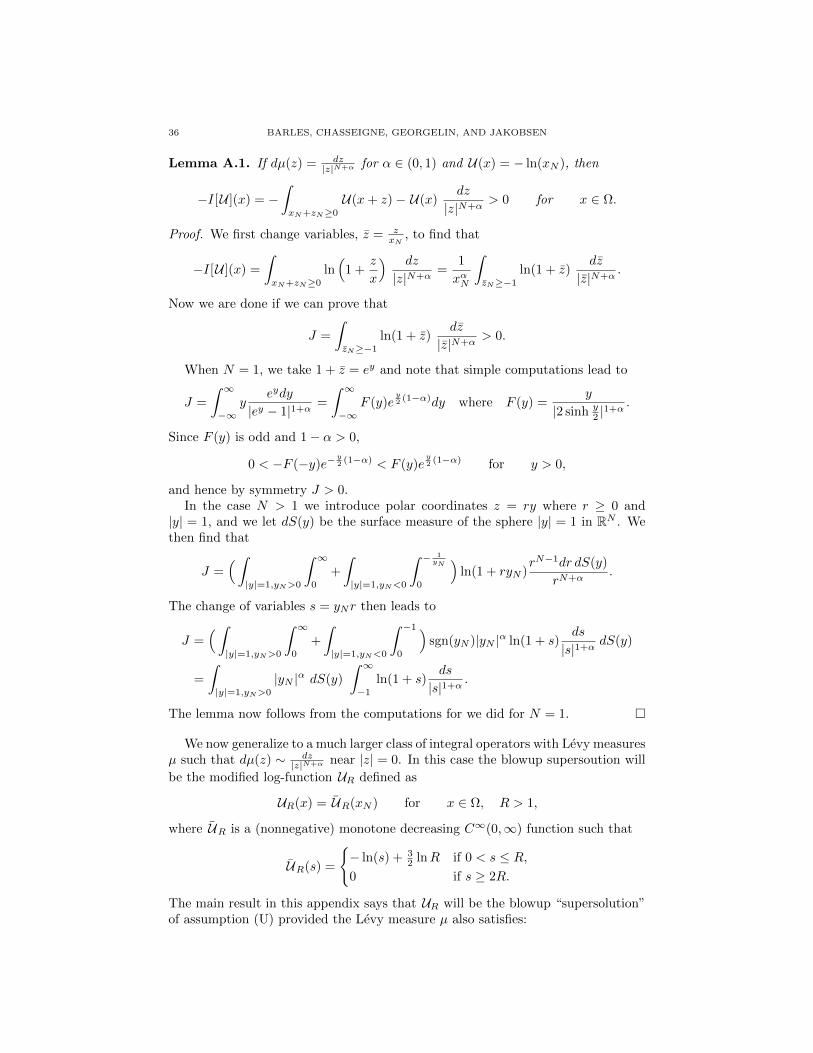
36 BARLES, CHASSEIGNE, GEORGELIN, AND JAKOBSEN
Lemma A.1. If dµ(z) = dz|z|N+α for α ∈ (0, 1) and U(x) = − ln(xN ), then
−I[U ](x) = −∫xN+zN≥0
U(x+ z)− U(x)dz
|z|N+α> 0 for x ∈ Ω.
Proof. We first change variables, z = zxN
, to find that
−I[U ](x) =
∫xN+zN≥0
ln(
1 +z
x
) dz
|z|N+α=
1
xαN
∫zN≥−1
ln(1 + z)dz
|z|N+α.
Now we are done if we can prove that
J =
∫zN≥−1
ln(1 + z)dz
|z|N+α> 0.
When N = 1, we take 1 + z = ey and note that simple computations lead to
J =
∫ ∞−∞
yeydy
|ey − 1|1+α=
∫ ∞−∞
F (y)ey2 (1−α)dy where F (y) =
y
|2 sinh y2 |1+α
.
Since F (y) is odd and 1− α > 0,
0 < −F (−y)e−y2 (1−α) < F (y)e
y2 (1−α) for y > 0,
and hence by symmetry J > 0.In the case N > 1 we introduce polar coordinates z = ry where r ≥ 0 and
|y| = 1, and we let dS(y) be the surface measure of the sphere |y| = 1 in RN . Wethen find that
J =(∫|y|=1,yN>0
∫ ∞0
+
∫|y|=1,yN<0
∫ − 1yN
0
)ln(1 + ryN )
rN−1dr dS(y)
rN+α.
The change of variables s = yNr then leads to
J =(∫|y|=1,yN>0
∫ ∞0
+
∫|y|=1,yN<0
∫ −1
0
)sgn(yN )|yN |α ln(1 + s)
ds
|s|1+αdS(y)
=
∫|y|=1,yN>0
|yN |α dS(y)
∫ ∞−1
ln(1 + s)ds
|s|1+α.
The lemma now follows from the computations for we did for N = 1.
We now generalize to a much larger class of integral operators with Levy measuresµ such that dµ(z) ∼ dz
|z|N+α near |z| = 0. In this case the blowup supersoution will
be the modified log-function UR defined as
UR(x) = UR(xN ) for x ∈ Ω, R > 1,
where UR is a (nonnegative) monotone decreasing C∞(0,∞) function such that
UR(s) =
− ln(s) + 3
2 lnR if 0 < s ≤ R,0 if s ≥ 2R.
The main result in this appendix says that UR will be the blowup “supersolution”of assumption (U) provided the Levy measure µ also satisfies:
NEUMANN PROBLEMS 37
(U)′ For all R, ε > 0 there are r, c,K > 0 and α ∈ (0, 1) such that
(a)
∫−1<zN≤R
ln(1 + zN )(sαµ(sdz)− c dz
|z|N+α
)> −ε for s ∈ (0, r),
(b)
∫−1<zN≤− 1
2
ln(1 + zN ) µ(sdz) ≥ −K for s ∈ (r,R).
Theorem A.2. Assume (H6η), (Hµ)′, and (U)′ hold. Then the function UR defined
above satisfy the assumptions in (U). In particular, there is R0 > 0 such that forany R > R0 there is KR ≥ 0 such that
−I[UR](x) ≥ −KR in x : 0 < xN ≤ R.Before we prove this result, we show how assumption (U)′ can be checked when
µ is Levy measure whos restriction to z : |zN | ≤ r has a density
dµ
dz=
g(z)
|z|N+αwhere
α ∈ (0, 1),
0 ≤ g ∈ L∞loc(RN ) ∩ L1(RN ; dz1+|z|N+α ),
limz→0 g(z) = g(0) > 0.
(A.1)
Note that the L1 assumption makes dµdz integrable near infinity and that L∞(RN ) ⊂
L1(RN ; dz1+|z|N+α ) for α > 0.
Corollary A.3. If µ has a density satisfying (A.1), then the function UR definedabove satisfy the assumptions in (U).
Proof. By Theorem A.2 we have to check that (U)′ holds. Part (b) follows fromHolder’s inequality since ln(1 + s) ∈ L1(−1, 0). Now we check part (a). Note that
sαµ(sdz)− c dz
|z|N+α=g(sz)− c|z|N+α
dz.
Now choose c = g(0) and write∫−1<zN≤R
ln(1 + zN )(sαµ(sdz)− c dz
|z|N+α
)≥ − sup
−s<r<Rs|g(r)− g(0)|
∫−1<zN≤R
| ln(1 + zN )| dz
|z|N+α.
Part (a) now follows since the last integral is finite for any R > 0, while the sup-termgoes to zero as s→ 0 by continuity of g at z = 0.
Remark A.1. Assumption (A.1) also includes measures like
µ =
M1∑i=1
µi,
where µi have densities satifying (A.1) for different gi and αi. To see this, simply
take α = maxi αi and g(z) =∑Mi=1 gi(z)|z|α−αi and note that g ∈ L1(RN ; dz
1+|z|N+α ).
We can even relax this assumption to include measures with zero or arbitrary neg-ative αi provided that maxi αi remains in (0, 1). Finally we mention that we needsome assumption to insure that µ does not give to much mass to the negative partof the integral −I[UR]. In (A.1) we do this by requiring continuity at 0 of g, but acarefull reader can extend this assumption to allow some discontinuities at 0.

38 BARLES, CHASSEIGNE, GEORGELIN, AND JAKOBSEN
Remark A.2. In assumption (U)′ it is only the restriction of µ to the set
z : −r < zN < Rr ∩ z : −1 < zN < −1
2
that plays any role. Hence if µ satisfies (U)′, by taking r small enough, so will µ+ µfor any measure µ satisfying∫
|z|>0
dµ <∞ and supp µ ∩ z : −1 < zN < r = ∅ for some r > 0.
E.g. the delta-measure µ =∑Mi=1 δxi is ok if xiN > 0.
Proof of Theorem A.2. First note that there is an R0 > 0 such that
JR0 :=
∫−1<zN≤R0
ln(1 + zN )dz
|z|N+α> 0.
Indeed, in the proof of Lemma A.1, we showed that J∞ = J > 0. The result thenfollows by the Dominated Convergence Theorem since the integrand is positive forzN > 0 and integrable.
For any R > R0, we note immediatly that UR is a nonnegative decreasing func-tion which trivially satisfies the second part of (U) with ωR(s) = 1
UR(s). We will
now check that UR has the appropriate supersolution properties and hence com-plete the proof that UR satisfies (U) under (U)′ . By the definition of UR, we canwrite
−I[UR](x) =
∫−xN<zN≤RxN
ln(
1 +zNxN
)µ(dz) + IR
=
∫−1<yN≤R
ln(1 + yN ) µ(xN dy) + IR,
where IR = −∫zN>RxN
UR(x + z) − UR(x) µ(dz) > 0 since UR is decreasing. By
assumption (U)′ we then find a r > 0 such that for xN ∈ (0, r),
−xαNI[UR](x) ≥ JR +
∫−1<yN≤R
ln(1 + y)(xαNµ(xN dy)− dy
|y|1+α
)≥ 1
2JR > 0.
When xN ∈ (r,R), another application of (U)′ along with (Hµ)′ leads to
− I[UR](x)
≥(∫−xN<zN<− xN2
+
∫− xN2 <zN<R∩|z|<1
+
∫− xN2 <zN<R∩|z|>1
)ln(
1 +z
xN
)dµ(dz)
≥ −K − maxs∈(− 1
2 ,Rr )
|∂s ln(1 + s)||xN |
∫|z|<1
|z|dµ(z)− maxs∈(− 1
2 ,Rr )| ln(1 + s)|
∫|z|>1
dµ(z).
Since this last expression is bounded for xN ∈ (r,R), this completes the proof.
Appendix B. Estimates for the censored case II.
Lemma B.1. Let µ(dz) = dz|z|N+α , α ∈ (1, 2), and define θ(x) = |xN |β. If β ∈ (0, 1)
and x ∈ Ω, then
I[θ](x) = P.V.
∫xN+zN≥0
θ(x+ z)− θ(x) µ(dz)
> 0 if β > α− 1,
= 0 if β = α− 1,
< 0 if β < α− 1.

NEUMANN PROBLEMS 39
Proof. First let β ∈ (0, 1) and N = 1, and define θ(x) = |x|β . Note that the changeof variables z = xz followed by 1 + z = es reveals that
I[θ](x) = P.V.
∫x+z≥0
|x+ z|β − |x|β dz
|z|1+α
= |x|β−α P.V.∫z≥−1
|1 + z|β − 1dz
|z|1+α
= |x|β−α P.V.∫ ∞−∞
2 sinh βs2
|2 sinh s2 |1+α
es2 (1+β−α)dx.
When β = α− 1, the integrand is odd and hence the integral is zero. For β > α− 1(β < α − 1) the exponential factor makes the integral positive (negative). Hence
when β + 1− α = 0, > 0 or < 0, then I[θ] = 0, > 0, or < 0 respectively.
When N > 1, a similar result holds for θ(x) = |xN |β . The idea is to work inpolar coordinates. We set x = ry for r ≥ 0 and |y| = 1 and let dS(y) denote thesurface area element of the N -sphere |y| = 1. We also use the change of variablesryN = rxN .
I[θ](x)
=
∫xN+zN≥0
|xN + zN |β − |xN |βdz
|z|N+α
=
∫|y|=1
∫xN+ryN>0
|xN + ryN |β − |xN |βrN−1dr dS(y)
rN+α
=
(∫|y|=1,yN>0
∫ ∞0
+
∫|y|=1,yN<0
∫ − xNyN0
)(· · · )dr dS(y)
r1+α
=
(∫|y|=1,yN>0
∫ ∞0
−∫|y|=1,yN<0
∫ −1
0
)|xN |β−α|yN |α
(|1 + r|β − 1
)dr dS(y)
|r|1+α
= |xN |β−α∫|y|=1,yN>0
|yN |α dS(y)
∫ ∞−1
|1 + r|β − 1dr
|r|1+α.
Here the first integral is just a positive constant while the second integral is thesame we found in the N = 1 case. The conclusion is therefore as in that case:When β + 1− α = 0, > 0 or < 0, then I[θ] = 0, > 0, or < 0 respectively.
Next we consider the two integrals
B(a) =
∫ −a−a−1
|1 + z|β − 1 dµ(z),
G =
∫ 1
−1
|1 + z|β + |1− z|β − 2 dµ(z),
where a > 1, β ∈ (0, 1), and dµ(z) = dz|z|N+α for α ∈ [1, 2).
Proposition B.2. If β = α− 1 then there is a κ > 0 such that
B(a) +G ≤ −κ < 0
for any a > 1.
By continuity of the integrals in β we have the following corollary:
40 BARLES, CHASSEIGNE, GEORGELIN, AND JAKOBSEN
Corollary B.3. There is κ > 0 and β > α− 1 such that
B(a) +G ≤ −κ ≤ 0
for any a > 1.
To prove Proposition B.2, note that z + 1 ≤ 0 for z ∈ (−a− 1,−a) (a > 1) andthat the change of variable 1 + z = −ex in B(a) leads to
B(a) =
∫ ln a
ln(a−1)
2 sinh βx2
|2 cosh x2 |1+α
ex2 (1+β−α) dx
β=α−1=
∫ ln a
ln(a−1)
2 sinh βx2
|2 cosh x2 |1+α
dx.
For the G integral we have the following result.
Lemma B.4.
G = 2 P.V.
∫ ln 2
− ln 2
2 sinh βx2
|2 sinh x2 |1+α
ex2 (1+β−α)dx − 2
∫ ∞ln 2
2 sinh βx2
|2 sinh x2 |1+α
e−x2 (1+β−α)dx,
and if β = α− 1,
G = − 2
∫ ∞ln 2
2 sinh βx2
|2 sinh x2 |1+α
dx.
Proof. First note that by symmetry
G = 2 limb→0+
∫(−1,1)\(−b,b)
|1 + z|β − 1 dµ(z).
Then, since 1 + z > 0 for z ∈ (−1, 1), the change of variable 1 + z = ex leads to
G = 2 limb→0+
∫(−∞,ln 2)\(ln(1−b),ln(1+b))
2 sinh βx2
|2 sinh x2 |1+α
ex2 (1+β−α) dx.
Note that ln(1± b) = ±b+O(b2) and decompose the above integral as follows,∫(−∞,ln 2)\(ln(1−b),ln(1+b))
(· · · ) dx
=(∫
(−∞,ln 2)\(−b,+b)+
∫(−∞,ln 2)\(ln(1−b),−b)
−∫
(−∞,ln 2)\(ln(1+b),b)
)(· · · ) dx
Now since sinhx = x + O(x3), the last two integrals are bounded by Cb2 bb1+α =
Cb2−α for b 1, and we have
G = 2 limb→0+
∫(−∞,ln 2)\(−b,b)
(· · · ) dx = 2
(P.V.
∫(− ln 2,ln 2)
+
∫(−∞,− ln 2)
)(· · · ) dx.
A change of variables in the last integral then gives the first statement of the Lemma.The last part of the lemma follows since the integrand is odd when β = α− 1, andhence the integral over (− ln 2, ln 2) vanishes.
We also need the next lemma.
Lemma B.5. If β = α− 1, then B(2) < −G2 .

NEUMANN PROBLEMS 41
Proof. We will show that
B(2) =
∫ ln 2
0
2 sinh βx2
|2 cosh x2 |1+α
dx ≤∫ ln 2
0
2 sinh β(x+ln 2)2
|2 sinh x+ln 22 |1+α
dx <
∫ ∞0
(· · · ) dx = −G2.
The last inequality is trivial, and since sinh is an increasing function, the firstinequaliy follows if we can show that
coshx
2≥ sinh
x+ ln 2
2for all x ∈ (0, ln 2).
But this easily follows since f(x) = cosh x2 − sinh x+ln 2
2 satisfy
f ′(x) =1
2sinh
x
2− 1
2cosh
x+ ln 2
2≤ 0 for all x,
f(ln 2) =
√2− 1
4≥ 0.
Proof of Proposition B.2. Divide the integral B(a) into three parts(∫ 0
ln(a−1)∧0
+
∫ ln 2∧ln a
ln(a−1)∨0
+
∫ ln 2∨ln a
ln 2
)(· · · ) dx.
Now we conclude since the first integral is negative, the second one is less than −G2by Lemma B.5, and the last one is less than −G2 by definition of G.
References
[1] D. Applebaum Levy Processes and Stochastic Calculus Cambridge University Press, Cam-
bridge, 2009.[2] G. Barles, E. Chasseigne, and C. Imbert. On the Dirichlet problem for second-order elliptic
integro-differential equations. Indiana Univ. Math. J. 57 (2008), no. 1, 213–246.
[3] G. Barles, C. Georgelin, and E. Jakobsen. On Neumann and oblique derivatives boundaryconditions for second-order elliptic integro-differential equations in preparation.
[4] G. Barles and C. Imbert. Second-order elliptic integro-differential equations: viscosity solu-
tions’ theory revisited. Ann. Inst. H. Poincare Anal. Non Lineaire 25 (2008), no. 3, 567-585.[5] G. Barles and P.L. Lions Remarques sur les problemes de reflexion oblique. C. R. Acad. Sci.
Paris Ser. I Math. 320 (1995), no. 1, 69–74.
[6] K. Bogdan, K. Burdzy and Z. Chen Censored stable processes Probab. Theory Related Fields127 (2003), no. 1, 89-152.
[7] L. Caffarelli and L. Silvestre. An extension problem related to the fractional Laplacian.Comm. Partial Differential Equations 32 (2007), no. 7-9, 1245–1260.
[8] R. Cont and P. Tankov. Financial modelling with jump processes. Chapman & Hall/CRC,
Boca Raton, FL, 2004.[9] M. Freidlin. Functional integration and partial differential equations. Annals of Mathematics
Studies, vol. 109, Princeton University Press, Princeton, 1985.
[10] M. Fukushima, Y. Oshima and M. Takeda Dirichlet forms and symmetric Markov processesde Grueter Studies in Mathematics 19 (1994)
[11] M.G. Garroni and J. L. Menaldi. Second order elliptic integro-differential problems. Chapman
& Hall/CRC Research Notes in Mathematics, 430. Chapman & Hall/CRC, Boca Raton, FL,2002.
[12] Q.Y. Guan. The integration by part of the regional fractional Laplacian. Commun. Math.
Phys. 266, 289–329 (2006)[13] Q.Y. Guan. and Z.M. Ma Reflected symmetric α stable process and regional fractional Lapla-
cian. Probab. Theory Relat. Fields 134, 649–694 (2006)[14] P. Hsu. On excursions of reflecting Brownian motions. Transactions of the A.M.S. 296, no
1(1996), 239–264
42 BARLES, CHASSEIGNE, GEORGELIN, AND JAKOBSEN
[15] J. L. Menaldi and M. Robin Reflected Diffusion Processes with Jumps The Annals of Prob-
ability, Vol. 13, No. 2 (May 1985), pp. 319-341
[16] N. Jacob. Pseudo differential operators and Markov process. Vol III . Markov process andApplications Imperial College Press, Princeton, 2005.
[17] P.-L. Lions and A.-S. Sznitman Stochastic differential equations with reflecting boundary
conditions. Comm. Pure Appl. Math. 37 (1984), no. 4, 511–537.[18] P.-L. Lions, J. L. Menaldi and A.-S. Sznitman Construction de processus de diffusion reflechis
par penalisation du domaine CRAS Paris I-292 , 559-562(1981).
[19] D. Stroock Diffusion processes associated with Levy generators, Z.Wahrscheinlichkeitstheorieund Verw. Gebiete 32 (1975), no. 3, 209?244..
[20] K. Taira Boundary value problems for elliptic integro-differential operators, Math. Z. 222,
305- 327 (1996).[21] K. Taira Semigroups, boundary value problems and Markov processes , Springer Monographs
in MAthematics, Springer Verlag (2003).
(Guy Barles) Laboratoire de Mathematiques et Physique Theorique, CNRS UMR 6083,Federation Denis Poisson, Universite Francois Rabelais, Parc de Grandmont, 37200
Tours, France
E-mail address: [email protected]
(Emmanuel Chasseigne) Laboratoire de Mathematiques et Physique Theorique, CNRS
UMR 6083, Federation Denis Poisson, Universite Francois Rabelais, Parc de Grand-mont, 37200 Tours, France
E-mail address: [email protected]
(Christine Georgelin) Laboratoire de Mathematiques et Physique Theorique, CNRSUMR 6083, Federation Denis Poisson, Universite Francois Rabelais, Parc de Grand-
mont, 37200 Tours, FranceE-mail address: [email protected]
(Espen R. Jakobsen) Department of Mathematical Sciences, Norwegian University of
Science and Technology, 7491 Trondheim, NorwayE-mail address: [email protected]