on model predictive control for economic and robust ... · pdf filede esta manera, varios...
TRANSCRIPT

On Model Predictive Control for
Economic and Robust Operation of
Generalised Flow-based Networks
Juan Manuel Grosso Perez
Institut de Robotica i Informatica Industrial
Universitat Politecnica de Catalunya. BarcelonaTech
Consejo Superior de Investigaciones Cientıficas
A thesis co-directed by:
Dr. Carlos Ocampo-MartınezDr. Vicenc Puig Cayuela
A thesis submitted for the degree of
Doctor of Philosophy
Barcelona, Spain, March 2015

Universitat Politecnica de Catalunya. BarcelonaTech
Departament d’Enginyeria de Sistemes, Automatica i Informatica Industrial
Doctoral Programme:Automatic Control, Robotics and Computer Vision (ARV)
This PhD thesis was completed at:
Institut de Robotica i Informatica Industrial, CSIC-UPC
Advisors:Dr. Carlos Ocampo-MartınezDr. Vicenc Puig Cayuela
External Reviewers:Dr. Bart De Schutter (Delft University of Technology)Dr. Alessandro Casavola (Universita della Calabria)
PhD Thesis Committee:Dr. Alessandro Casavola (Universita della Calabria)Dr. Sorin Olaru (SUPELEC)Dr. Gabriela Cembrano (Consejo Superior de Investigaciones Cientıficas)Dr. Francesco Tedesco (Universita della Calabria)Dr. Ramon Perez (Universitat Politecnica de Catalunya)
c© Juan Manuel Grosso Perez 2015

To my family...


Acknowledgements
There is a point in time where certain things have to end to set ourselves at the beginningof an open highway of new opportunities and challenges to be faced, thus, now is myturn to give end to my doctoral thesis. This dissertation represents not only my workat the boards, papers and computers during the last four years but also a bunch ofups and downs, professional and personal experiences that have shaped my life and myknowledge. This journey has not been made in loneliness and here I want to express mysincere gratitude to those that supported me during my doctoral days.
First, I want to thank my supervisors Dr. Carlos Ocampo-Martinez and Prof. VicencPuig for their continuous support. They gave me the possibility to start this challengingjourney and a place for learning with freedom for professional development within thecontext of applied research.
Second, I want to thank Prof. Frank Allgower from the Institute for Systems The-ory and Automatic Control of the University of Stuttgart for receiving me as a visitorresearcher and for giving me a place and the opportunity to interact with excellent re-searchers. Special thanks go to Dr. Matthias Muller for his time to discuss and make meanalyse interesting issues regarding economic MPC, even when he was fully consumedby the writing of his own PhD thesis. In the same way, I want to thank Dr. DanielLimon and Dr. Jose Marıa Maestre, both of them from University of Seville, and Dr.Pantelis Sopasakis from IMT Lucca for our technical discussions and for our commonresearch activities. Thanks to all of them I complemented some contents of this thesis.
Third, I wish to express my gratitude to Prof. Bart De Schutter from TU Delftand Prof. Alessandro Casavola from University of Calabria for having reviewed thethesis, providing helpful comments to improve the quality of the manuscript. Moreover,I want to thank Prof. Casavola, in addition to Prof. Sorin Olaru from SUPELEC,Dr. Gabriela Cembrano from CSIC, Dr. Francesco Tedesco from University of Calabriaand Dr. Ramon Perez from UPC for joining my thesis committee.
Fourth, I would like to thank some people I met at IRI, with whom I founded not onlya scientific and academic relationship with fruitful discussions but also ties of friendshipthat allowed me to research in a pleasant working environment. Special thanks to FengXu, Albert Rosich, Bernat Joseph, Stephan Strahl and Maite Urrea, with whom I hadinteresting talks ranging from how to do research to topics related to history, music,economy, etc.
Fifth, I want to thank the projects that funded my research. The work presentedin this thesis has been partially supported by the EU projects EFFINET (FP7-ICT-2011-8-31855) and i-Sense (FP7-ICT-2009-6-270428), and by the Spanish projects ECO-CIS (CICYT DPI2013-48243-C2-1-R) and SHERECS (CICYT DPI2011-26243) of theMinistry of Economy and Competitiveness, WATMAN (CICYT DPI2009-13744) of the
iii

Ministry of Science and Technology and the DGR of Generalitat de Catalunya (SACgroup Ref. 2014/SGR/374).
Finally, I owe my gratitude to my family for being such a great example of work,courage and perseverance, for their support and motivation despite the distance duringthese years. Especially, I want to express my deepest thankfulness to Fernanda, for herunlimited love and support during the not always easy time as a PhD student; theseyears has been coloured with her company and she has given me the strength to fightfor this achievement.
Juan Manuel GrossoBarcelona, February 2015
iv

Abstract
This thesis is devoted to design Model Predictive Control (MPC) strategies aimingto enhance the management of constrained generalised flow-based networks, with spe-cial attention to the economic optimisation and robust performance of such systems.Several control schemes are developed in this thesis to exploit the available economicinformation of the system operation and the disturbance information obtained frommeasurements and forecasting models. Dynamic network flows theory is used to de-velop control-oriented models that serve to design MPC controllers specialised for flownetworks with additive disturbances and periodically time-varying dynamics and costs.The control strategies developed in this thesis can be classified in two categories: cen-tralised MPC strategies and non-centralised MPC strategies. Such strategies are assessedthrough simulations of a real case study: the Barcelona drinking water network (DWN).
Regarding the centralised strategies, different economic MPC formulations are firststudied to guarantee recursive feasibility and stability under nominal periodic flow de-mands and possibly time-varying economic parameters and multi-objective cost func-tions. Additionally, reliability-based MPC, chance-constrained MPC and tree-basedMPC strategies are proposed to address the reliability of both the flow storage and theflow transportation tasks in the network. Such strategies allow to satisfy a customerservice level under future flow demand uncertainty and to efficiently distribute over-all control effort under the presence of actuators degradation. Moreover, soft-controltechniques such as artificial neural networks and fuzzy logic are used to incorporateself-tuning capabilities to an economic certainty-equivalent MPC controller.
Since there are objections to the use of centralised controllers in large-scale net-works, two non-centralised strategies are also proposed. First, a multi-layer distributedeconomic MPC strategy of low computational complexity is designed with a controltopology structured in two layers. In a lower layer, a set of local MPC agents are incharge of controlling partitions of the overall network by exchanging limited informationon shared resources and solving their local problems in a hierarchical-like fashion. More-over, to counteract the loss of global economic information due to the decompositionof the overall control task, a coordination layer is designed to influence non-iterativelythe decision of local controllers towards the improvement of the overall economic per-formance. Finally, a cooperative distributed economic MPC formulation based on aperiodic terminal cost/region is proposed. Such strategy guarantees convergence to aNash equilibrium without the need of a coordinator and relies on an iterative and globalcommunication of local controllers, which optimise in parallel their control actions butusing a centralised model of the network.
Keywords: MPC, economic optimisation, robust performance, reliability, centralisedcontrol, distributed control, non-iterative coordination, cooperative control.
v


Resumen
Esta tesis se enfoca en el diseno de estrategias de control predictivo basado en mod-elos (MPC, por sus siglas en ingles) con la meta de mejorar la gestion de sistemas quepueden ser descritos por redes generalizadas de flujo y que estan sujetos a restricciones,enfatizando especialmente en la optimizacion economica y el desempeno robusto de talessistemas. De esta manera, varios esquemas de control se desarrollan en esta tesis paraexplotar tanto la informacion economica disponible de la operacion del sistema como lainformacion de perturbaciones obtenida de datos medibles y de modelos de prediccion.La teorıa de redes dinamicas de flujo es utilizada en esta tesis para desarrollar modelosorientados a control que sirven para disenar controladores MPC especializados para lagestion de redes de flujo que presentan tanto perturbaciones aditivas como dinamicas ycostos periodicamente variables en el tiempo. Las estrategias de control propuestas enesta tesis se pueden clasificar en dos categorıas: estrategias de control MPC centralizadoy estrategias de control MPC no-centralizado. Dichas estrategias son evaluadas medi-ante simulaciones de un caso de estudio real: la red de transporte de agua potable deBarcelona en Espana.
En cuanto a las estrategias de control MPC centralizado, diferentes formulacionesde controladores MPC economicos son primero estudiadas para garantizar factibilidadrecursiva y estabilidad del sistema cuya operacion responde a demandas nominales deflujo periodico, a parametros economicos posiblemente variantes en el tiempo y a fun-ciones de costo multi-objetivo. Adicionalmente, estrategias de control MPC basado enfiabilidad, MPC con restricciones probabilısticas y MPC basado en arboles de escenariosson propuestas para garantizar la fiabilidad tanto de tareas de almacenamiento como detransporte de flujo en la red. Tales estrategias permiten satisfacer un nivel de servicioal cliente bajo incertidumbre en la demanda futura, ası como distribuir eficientemente elesfuerzo global de control bajo la presencia de degradacion en los actuadores del sistema.Por otra parte, tecnicas de computacion suave como redes neuronales artificiales y logicadifusa se utilizan para incorporar capacidades de auto-sintonıa en un controlador MPCeconomico de certeza-equivalente.
Dado que hay objeciones al uso de control centralizado en redes de gran escala, dosestrategias de control no-centralizado son propuestas en esta tesis. Primero, un con-trolador MPC economico distribuido de baja complejidad computacional es disenadocon una topologıa estructurada en dos capas. En una capa inferior, un conjunto decontroladores MPC locales se encargan de controlar particiones de la red mediante elintercambio de informacion limitada de los recursos fısicos compartidos y resolviendosus problemas locales de optimizacion de forma similar a una secuencia jerarquica desolucion. Para contrarrestar la perdida de informacion economica global que ocurre trasla descomposicion de la tarea de control global, una capa de coordinacion es disenadapara influenciar no-iterativamente la decision de los controles locales con el fin de lo-
vii

grar una mejora global del desempeno economico. La segunda estrategia no-centralizadapropuesta en esta tesis es una formulacion de control MPC economico distribuido cooper-ativo basado en una restriccion terminal periodica. Tal estrategia garantiza convergenciaa un equilibrio de Nash sin la necesidad de una capa de coordinacion pero requiere unacomunicacion iterativa de informacion global entre todos los controladores locales, loscuales optimizan en paralelo sus acciones de control utilizando un modelo centralizadode la red.
Palabras clave: MPC, optimizacion economica, desempeno robusto, fiabilidad, con-trol centralizado, control distribuido, coordinacion no-iterativa, control cooperativo.
viii

Contents
Acknowledgements iii
Abstract vii
Resumen ix
List of Figures xvii
List of Tables xxi
Nomenclature xxiii
I Preliminaries 1
1 Introduction 3
1.1 Motivation . . . . . . . . . . . . . . . . . . . . . . . . . . . . . . . . . . . 3
1.2 Research Background . . . . . . . . . . . . . . . . . . . . . . . . . . . . . 6
1.2.1 Reliability in Flow-based Networks . . . . . . . . . . . . . . . . . . 7
1.2.2 Decision Making under Uncertainty . . . . . . . . . . . . . . . . . 9
1.2.3 MPC Tuning Strategies . . . . . . . . . . . . . . . . . . . . . . . . 12
1.2.4 Economic MPC for the Management of Network Flows . . . . . . . 13
1.2.5 Non-centralised MPC for Large-scale Networks . . . . . . . . . . . 15
1.3 Thesis Objectives . . . . . . . . . . . . . . . . . . . . . . . . . . . . . . . . 18
ix

CONTENTS
1.4 Outline of the Thesis . . . . . . . . . . . . . . . . . . . . . . . . . . . . . . 19
2 Generalised Flow-based Networks 25
2.1 Introduction . . . . . . . . . . . . . . . . . . . . . . . . . . . . . . . . . . . 25
2.2 Modelling and Problem Statement . . . . . . . . . . . . . . . . . . . . . . 27
2.2.1 Networks as Directed Graphs . . . . . . . . . . . . . . . . . . . . . 27
2.2.2 Network Attributes . . . . . . . . . . . . . . . . . . . . . . . . . . . 28
2.2.3 Dynamic Minimum Cost Flow Problem . . . . . . . . . . . . . . . 30
2.3 Integrating Scheduling and Control . . . . . . . . . . . . . . . . . . . . . . 32
2.3.1 Control-oriented Model . . . . . . . . . . . . . . . . . . . . . . . . 33
2.3.2 MPC for the Control of Dynamic Network Flows . . . . . . . . . . 36
2.4 Case Study . . . . . . . . . . . . . . . . . . . . . . . . . . . . . . . . . . . 39
2.4.1 Description . . . . . . . . . . . . . . . . . . . . . . . . . . . . . . . 39
2.4.2 System Management Criteria . . . . . . . . . . . . . . . . . . . . . 40
2.4.3 Baseline MPC Problem Setting . . . . . . . . . . . . . . . . . . . . 44
2.4.4 Key Performance Indicators . . . . . . . . . . . . . . . . . . . . . . 47
2.5 Numerical Results . . . . . . . . . . . . . . . . . . . . . . . . . . . . . . . 47
2.6 Summary . . . . . . . . . . . . . . . . . . . . . . . . . . . . . . . . . . . . 49
II Centralised MPC Schemes for Economic and Robust Operation 53
3 Economic MPC Strategies for Generalised Flow-based Networks 55
3.1 Introduction . . . . . . . . . . . . . . . . . . . . . . . . . . . . . . . . . . . 55
3.2 Problem Statement . . . . . . . . . . . . . . . . . . . . . . . . . . . . . . . 56
3.3 Existence of Admissible Controlled Flows . . . . . . . . . . . . . . . . . . 59
3.4 Synthesis of Flow-based Controllers . . . . . . . . . . . . . . . . . . . . . . 63
3.4.1 Economic Scheduling Optimisation for Periodic Operation . . . . . 63
x

CONTENTS
3.4.2 Nominal Economic MPC Strategies for Periodic Network Flows . . 64
3.4.3 Numerical Results . . . . . . . . . . . . . . . . . . . . . . . . . . . 70
3.5 Economic MPC for Periodic Systems . . . . . . . . . . . . . . . . . . . . . 74
3.5.1 Economically Optimal Scheduling for Periodic Systems . . . . . . . 75
3.5.2 Economic MPC with Periodic Terminal Penalty and Region . . . . 76
3.5.3 Analysis of the Average Performance . . . . . . . . . . . . . . . . . 78
3.5.4 Lyapunov Nominal Stability . . . . . . . . . . . . . . . . . . . . . . 80
3.5.5 Computation of the Terminal Ingredients . . . . . . . . . . . . . . 84
3.5.6 Numerical Results . . . . . . . . . . . . . . . . . . . . . . . . . . . 91
3.6 Summary . . . . . . . . . . . . . . . . . . . . . . . . . . . . . . . . . . . . 94
4 Reliability-based MPC of Generalised Flow-based Networks 97
4.1 Introduction . . . . . . . . . . . . . . . . . . . . . . . . . . . . . . . . . . . 97
4.2 Safety Stocks Allocation Policy . . . . . . . . . . . . . . . . . . . . . . . . 99
4.3 Actuator Health Management Policy . . . . . . . . . . . . . . . . . . . . . 101
4.4 Reliability-based Economic MPC Problem . . . . . . . . . . . . . . . . . . 103
4.5 Numerical Results . . . . . . . . . . . . . . . . . . . . . . . . . . . . . . . 105
4.6 Summary . . . . . . . . . . . . . . . . . . . . . . . . . . . . . . . . . . . . 111
5 Stochastic MPC for Robustness in Generalised Flow-based Networks 113
5.1 Introduction . . . . . . . . . . . . . . . . . . . . . . . . . . . . . . . . . . . 113
5.2 Problem Formulation . . . . . . . . . . . . . . . . . . . . . . . . . . . . . . 115
5.3 Chance-Constrained MPC . . . . . . . . . . . . . . . . . . . . . . . . . . . 117
5.4 Tree-based MPC . . . . . . . . . . . . . . . . . . . . . . . . . . . . . . . . 122
5.5 Numerical Results . . . . . . . . . . . . . . . . . . . . . . . . . . . . . . . 124
5.6 Summary . . . . . . . . . . . . . . . . . . . . . . . . . . . . . . . . . . . . 144
xi

CONTENTS
6 Learning-based Tuning of Supervisory MPC for Generalised Flow-based Networks 147
6.1 Control System Structure . . . . . . . . . . . . . . . . . . . . . . . . . . . 148
6.2 Learning and Planning Layer . . . . . . . . . . . . . . . . . . . . . . . . . 148
6.2.1 ANN for Demand Forecasting . . . . . . . . . . . . . . . . . . . . . 150
6.2.2 ANN for Optimal Economic Trajectory . . . . . . . . . . . . . . . 151
6.2.3 ANN for Dynamical Safety Volumes . . . . . . . . . . . . . . . . . 152
6.3 Supervision and Adaptation Layer . . . . . . . . . . . . . . . . . . . . . . 152
6.3.1 Reasoning Mechanism . . . . . . . . . . . . . . . . . . . . . . . . . 153
6.3.2 Linking Heuristic . . . . . . . . . . . . . . . . . . . . . . . . . . . . 155
6.4 Numerical Results . . . . . . . . . . . . . . . . . . . . . . . . . . . . . . . 156
6.4.1 Demand Forecasting and States Planning with ANNs . . . . . . . 156
6.4.2 Fuzzy Tuning of MPC Parameters . . . . . . . . . . . . . . . . . . 157
6.4.3 LB-MPC Controller for DWN . . . . . . . . . . . . . . . . . . . . . 157
6.5 Summary . . . . . . . . . . . . . . . . . . . . . . . . . . . . . . . . . . . . 162
III Distributed Economic MPC Schemes for Network Management163
7 Multi-Layer Non-Iterative Distributed Economic MPC 165
7.1 Introduction . . . . . . . . . . . . . . . . . . . . . . . . . . . . . . . . . . . 165
7.2 Problem Formulation . . . . . . . . . . . . . . . . . . . . . . . . . . . . . . 168
7.3 Description of the Approach . . . . . . . . . . . . . . . . . . . . . . . . . . 172
7.3.1 Lower Optimisation Layer . . . . . . . . . . . . . . . . . . . . . . . 172
7.3.2 Upper Optimisation Layer . . . . . . . . . . . . . . . . . . . . . . . 176
7.3.3 ML-DMPC Algorithm . . . . . . . . . . . . . . . . . . . . . . . . . 179
7.4 Numerical Results . . . . . . . . . . . . . . . . . . . . . . . . . . . . . . . 182
7.5 Summary . . . . . . . . . . . . . . . . . . . . . . . . . . . . . . . . . . . . 185
xii

CONTENTS
8 Distributed Economic MPC with Global Communication 189
8.1 Introduction . . . . . . . . . . . . . . . . . . . . . . . . . . . . . . . . . . . 189
8.2 Problem Formulation . . . . . . . . . . . . . . . . . . . . . . . . . . . . . . 191
8.3 Cooperative Distributed Economic MPC Formulation based on a Periodic
Terminal Penalty and Region . . . . . . . . . . . . . . . . . . . . . . . . . 193
8.4 Numerical Results . . . . . . . . . . . . . . . . . . . . . . . . . . . . . . . 197
8.5 Summary . . . . . . . . . . . . . . . . . . . . . . . . . . . . . . . . . . . . 199
IV Concluding Remarks 201
9 Concluding Remarks 203
9.1 Contributions . . . . . . . . . . . . . . . . . . . . . . . . . . . . . . . . . . 203
9.2 Directions for Future Research . . . . . . . . . . . . . . . . . . . . . . . . 206
V Appendices 209
A Demand Modelling 211
A.1 Water Demand Characterisation . . . . . . . . . . . . . . . . . . . . . . . 211
A.2 BATS Modelling of Water Demand . . . . . . . . . . . . . . . . . . . . . . 212
B Reduction of Flow Variables 217
C Convex Approximation of DWN Chance Constraints 219
D Background on LMIs 221
References 223
xiii


List of Figures
2.1 Example of a network directed graph. Source nodes (green), sink nodes
(red), intermediate nodes (blue) . . . . . . . . . . . . . . . . . . . . . . . . 28
2.2 Characterisation of network nodes . . . . . . . . . . . . . . . . . . . . . . 28
2.3 Barcelona DWN full diagram . . . . . . . . . . . . . . . . . . . . . . . . . 41
2.4 Barcelona DWN aggregate diagram . . . . . . . . . . . . . . . . . . . . . . 42
2.5 Barcelona DWN sector diagram . . . . . . . . . . . . . . . . . . . . . . . . 43
2.6 CE-MPC receding horizon strategy with hard and soft constraints . . . . 46
2.7 Management of water storage with the CE-MPC strategy . . . . . . . . . 51
2.8 Optimal operation of a sample of actuators in the Barcelona DWN . . . . 52
3.1 Price-of-use for actuators u4, u5 and u6 in economic units (e.u.) . . . . . . 73
3.2 Evolution of some states under varying economic parameters . . . . . . . 73
3.3 Graphical illustration of the proposed economic MPC with periodic ter-
minal region for the case n = 2, N = 8, T = 4. optimal periodic orbit
(dashed red), predicted state trajectory (dashed green), closed-loop state
trajectory (solid black). . . . . . . . . . . . . . . . . . . . . . . . . . . . . 90
4.1 Reliability-based MPC structure . . . . . . . . . . . . . . . . . . . . . . . 98
4.2 Management of storage of water with the RB-MPC strategies . . . . . . . 108
4.3 Management of actuators with the RB-MPC strategies . . . . . . . . . . . 109
xv

LIST OF FIGURES
4.4 Control actions for a sample of redundant actuators using the RB-MPC(2)
strategy . . . . . . . . . . . . . . . . . . . . . . . . . . . . . . . . . . . . . 110
4.5 Example of the smart tuning strategy within the RB-MPC(2) strategy . . 110
5.1 Reduction of a disturbance fan (left) of equally probable scenarios into a
rooted scenario-tree (right). . . . . . . . . . . . . . . . . . . . . . . . . . . 123
5.2 Comparison of the robustness in the management of water storage in a
sample of tanks of the Barcelona DWN: (blue circle) CC-MPC1%, (black
diamond) CC-MPC20%, (red square) CC-MPC50%, (solid green) CE-MPC,
(dashed red) Net demand. . . . . . . . . . . . . . . . . . . . . . . . . . . . 133
5.3 Operation of the Barcelona DWN with the CC-MPC strategies . . . . . . 136
5.4 Degradation of a set of redundant actuators under the CC-MPC strategies 137
5.5 Risk averse mechanism using RB-MPC and CC-MPC . . . . . . . . . . . 140
5.6 Comparison of hourly and daily costs . . . . . . . . . . . . . . . . . . . . . 142
6.1 Multilayer hierarchical intelligent control architecture . . . . . . . . . . . 149
6.2 Feed-forward Neural Network diagram . . . . . . . . . . . . . . . . . . . . 150
6.3 ANNs training diagrams for Demand Forecasting (top), Economic trajec-
tory (middle) and Base-stocks setting (bottom) . . . . . . . . . . . . . . . 151
6.4 Fuzzy rules-based MPC tuner diagram . . . . . . . . . . . . . . . . . . . . 153
6.5 Evolution of tuning parameters for the LB-MPC strategy . . . . . . . . . 158
6.6 Histograms of tuning parameters for the LB-MPC strategy . . . . . . . . 159
6.7 Dynamic variation of tanks volumes for the different approaches . . . . . 160
6.8 Comparison of the daily electric and water costs for the different approaches161
7.1 Decomposition of a network with r sources into M subsystems . . . . . . 169
7.2 ML-DMPC control architecture . . . . . . . . . . . . . . . . . . . . . . . . 173
7.3 Partition of the Barcelona DWN . . . . . . . . . . . . . . . . . . . . . . . 183
7.4 Network subsystems Si and their shared connections wij . . . . . . . . . . 184
xvi

LIST OF FIGURES
7.5 Total flow per water source in the Barcelona DWN . . . . . . . . . . . . . 186
7.6 Economic costs of the three MPC strategies . . . . . . . . . . . . . . . . . 186
8.1 Open-loop cost decreasing of VN as function of the number of Gauss-
Jacobi iterations . . . . . . . . . . . . . . . . . . . . . . . . . . . . . . . . 198
A.1 Histogram of demand c176BARsud in the Barcelona DWN . . . . . . . . 212
A.2 Time series decomposition by the BATS model for water demand fore-
casting in the Barcelona DWN . . . . . . . . . . . . . . . . . . . . . . . . 213
A.3 Forecasting of water demand using a BATS model . . . . . . . . . . . . . 213
xvii


List of Tables
2.1 Comparison of considered drinking water network configurations . . . . . 40
2.2 Key performance indicators for the CE-MPC strategy . . . . . . . . . . . 48
2.3 Water and electric cost for the CE-MPC strategy . . . . . . . . . . . . . . 48
3.1 Comparison of controller performance . . . . . . . . . . . . . . . . . . . . 71
3.2 Comparison of daily average costs of EMPC strategies . . . . . . . . . . . 72
3.3 Open-loop average cost of MPC strategies . . . . . . . . . . . . . . . . . . 93
3.4 Closed-loop performance of periodic economic MPC strategies . . . . . . . 94
4.1 Key performance indicators for RB-MPC . . . . . . . . . . . . . . . . . . 106
4.2 Water and electric cost comparison of RB-MPC strategies . . . . . . . . . 106
5.1 Assessment of CC-MPC and TB-MPC applied to the sector model of the
DWN case study. . . . . . . . . . . . . . . . . . . . . . . . . . . . . . . . . 129
5.2 Comparison of the MPC strategies applied to the Barcelona DWN . . . . 132
5.3 Comparison of daily average economic costs of MPC strategies . . . . . . 134
5.4 Key performance indicators for CC-MPC . . . . . . . . . . . . . . . . . . 135
5.5 Water and electric cost comparison of CC-MPC strategies . . . . . . . . . 138
5.6 Conservatism of the Deterministic Equivalent CC-MPC . . . . . . . . . . 139
5.7 Comparison of controllers performance . . . . . . . . . . . . . . . . . . . . 141
5.8 Comparison of daily average costs of MPC strategies . . . . . . . . . . . . 142
xix

LIST OF TABLES
5.9 Comparison of capabilities handled by each controller . . . . . . . . . . . 143
6.1 Fuzzy-logic rules for LB-MPC. . . . . . . . . . . . . . . . . . . . . . . . . 154
6.2 Performance of the ANNs (MAE%) . . . . . . . . . . . . . . . . . . . . . . 156
6.3 Key performance indicators for the different approaches . . . . . . . . . . 160
7.1 Performance comparisons . . . . . . . . . . . . . . . . . . . . . . . . . . . 185
8.1 Performance comparisons . . . . . . . . . . . . . . . . . . . . . . . . . . . 199
xx

Nomenclature
Notation
Symbol Description
·, . . . set or sequence
∅ empty set
x ∈ X x is an element of the set XR set of real numbers
R+ set of non-negative real numbers
R>c R>c := x ∈ R | x > c for some c ∈ R+
R≥c R≥c := x ∈ R | x ≥ c for some c ∈ R+
Rn space of n-dimensional (column) vectors with real entries
Rn×m space of n by m matrices with real entries
Z set of integers
Z+ set of non-negative integers including zero
Z>c Z>c := x ∈ Z | x > c for some c ∈ Z+
Z≥c Z≥c := x ∈ Z | x ≥ c for some c ∈ Z+
Z[c1,c2) Z[c1,c2) := x ∈ Z | c1 ≤ x < c2 for some c1, c2 ∈ Z+
Z[c1,c2] Z[c1,c2] := x ∈ Z | c1 ≤ x ≤ c2 for some c1, c2 ∈ Z+
X(⊂) ⊆ Y set X is a (strict) subset of YX× Y Cartesian product of the sets X and Y, i.e., X× Y = (x, y) | x ∈ X, y ∈ YXN N -dimensional Cartesian product X× X× . . .× X, for some N ∈ Z≥1
CoX convex hull of the set Xint(X) interior of the set Xx> (X>) transpose of a vector x ∈ Rn (matrix X ∈ Rn×m)
X−1 inverse of the matrix X ∈ Rn×n
xxi

NOMENCLATURE
x(i) (X(i)) i-th element (row) of the vector x ∈ Rn (matrix X ∈ Rn×m)
Xij element in the i-th row and j-th column of the matrix X ∈ Rn×m
xii∈Z[a,b]ordered sequence of elements (xa, . . . , xb) with a, b ∈ Z≥1 and a < b
diag(·) operator that builds a diagonal matrix with the elements of its argument
| · | (1) |x| ≥ 0 with x ∈ R returns the absolute value of the scalar x
(2) |x| ∈ (R+ ∪ 0)n returns the component-wise absolute value
of the vector x ∈ Rn
(3) |A| returns the cardinality of the set A
‖ · ‖ 2-norm (Euclidian norm) of a vector, i.e., ‖x‖ :=√∑n
i=1 x2(i), where x ∈ Rn
In identity matrix of dimension n× n, where n ∈ Z≥1
0m×n zero matrix of dimension m× n, where m,n ∈ Z≥1
Sn set of all n-dimensional symmetric matrices, i.e.,
Sn := X ∈ Rn×n | X = X>Sn+ (Sn−) set of all n-dimensional positive (negative) semi-definite matrices
Sn++ (Sn−−) set of all n-dimensional positive (negative) definite matrices
X 0 (≺ 0) X is a positive (negative) definite matrix, i.e., X ∈ Sn++
X 0 ( 0) X is a positive (negative) semi-definite matrix, i.e., X ∈ Sn+bicj bicj := mod(i, j) is the modulo operation between integers i, j ∈ Z+
P[·] probability measure
E[·] expectation with respect to probability measure P[·]N(x,Σx) multivariate normal distribution of x with mean x and covariance Σx
Φ(·) standard cumulative distribution function
Φ−1(·) quantile function
σx standard deviation of x
∂f∂x partial derivative of function f with respect to x[a ?b c
]the symbol ”?” denotes the symmetric part of a matrix,
i.e.,
[a ?b c
]=
[a b>
b c
]
xxii

NOMENCLATURE
Acronyms
Acronym Description
MPC Model Predictive Control
EMPC Economic Model Predictive Control
CE-MPC Certainty-Equivalent Model Predictive Control
RB-MPC Reliability-Based Model Predictive Control
SMPC Stochastic Model Predictive Control
CC-MPC Chance-Constrained Model Predictive Control
TB-MPC Tree-Based Model Predictive Control
LB-MPC Learning-Based Model Predictive Control
ML-DMPC Multi-Layer Distributed Model Predictive Control
CDEMPC Cooperative Distributed Economic Model Predictive Control
FHOP Finite Horizon Optimisation Problem
LMI Linear Matrix Inequality
LTI Linear Time Invariant
RTO Real-Time Optimiser
QP Quadratic Programming
LP Linear Programming
PID Proportional-Integral-Derivative
DWN Drinking Water Network
xxiii


Part I
Preliminaries
1


Chapter 1
Introduction
1.1 Motivation
The evolution of human civilisations until the current days might be heavily related to
the understanding and acceptance of connectivity and networks as tools to enhance the
quality of life, considering the importance of both social interactions and physical in-
frastructure systems. In the daily living people are part of many instances of networks,
e.g., communication networks, electrical power networks, public transport networks,
road-traffic networks, water networks, financial networks, supply-chains, among others.
These networks may be considered as critical infrastructures [122], since their proper op-
eration is vital for the normal functioning of modern society. Consequently, maintaining
a truly efficient, reliable and sustainable service is a must in network systems.
Physical networks are conceived and designed to supply different specific services.
Nevertheless, many of the problems that drive their operation (e.g., minimisation of
displacement times, maximisation of plants’ throughput, minimisation of energy con-
sumption, maximisation of demand satisfaction, etc.) share a common feature: some
commodity (or many at the same time), e.g., information, water, oil, money, people,
products, among any other real or abstract entity, need to be transported through the
network infrastructure, and this has to be done whilst making best use of available re-
sources and in line with the prevailing regulatory framework. Such similarity in the
related transportation problems gave rise to the classic field of network flows [2], which
forms a large area of optimisation theory (especially in combinatorial and linear program-
ming techniques) and are core problems in operations research, applied mathematics,
3

Chapter 1. Introduction
computer science, and many fields of engineering.
Under the framework of network flows, any network can be generically described with
a graph consisting of a set of nodes (or vertices) that represent locations, and a set of
arcs (or edges) that model links between nodes. The network nodes can be classified in
supply nodes (e.g., production units, oilfields, water reservoirs, factories), demand nodes
(e.g., houses, refineries, or other consumption points), and intermediate transshipment
nodes with or without storage capability (e.g., pipe junctions, pumping stations, street
crossings, warehouses, water storage deposits, energy storage units). Ordered sequences
of arcs (e.g., pipelines, electrical cables, roads, railways, or other channels) form paths
(or routes), which are used to transport the commodity from the supply nodes to the
demand nodes. Typically, nodes and arcs of a network are subject to capacity constraints
and to some costs associated with their use. The commodity that is being transported
over the network, however, determines how the overall system operates.
Network flow problems have been in the focus of research for many years and a ma-
ture theory for network analysis and design has been developed with numerous efficient
algorithms for solving classical problems such as the minimum cost flow problem, the
shortest path problem and the maximum flow problem. A comprehensive discussion of
theory, algorithms and applications of network flow problems can be found in [2, 17, 154].
Nevertheless, despite the mature mathematical background supporting the network flows
field, there are some aspects that limit the applicability of the available results to real
problems. To start, the main drawback of the classical network flow theory is that most
developed algorithms rely on the assumptions of static flow conditions and static net-
work structures, but time plays a vital role in many real applications, where capacities,
costs, supplies, demands, and therefore flows, evolve over time with possibly different
time scales. On other hand, static network flows theory does not consider in general
the possibility of storage in transshipment nodes nor the flow of multiple commodities,
which are crucial in several real networks.
The aforesaid weaknesses of static network flows have originated the so-called dy-
namic network flows (also called network flows over time). In general, dynamic network
flows have three main differences with respect to the traditional models; these differ-
ences are: (i) flows change over time, (ii) the flow between two nodes takes a finite
4

Chapter 1. Introduction
transit time and, (iii) storage is allowed at the nodes of the network for later trans-
portation. A further extension of the static and dynamic network flows is the so-called
generalised network flows, which allow to have gains in the arcs of the network. Dynamic
networks were introduced in [59, 85]. Since then, several authors have studied different
features of flows over time and useful surveys on the topic are available in the literature,
see e.g., [9, 80, 95, 97, 168]. A common conclusion reported in the aforementioned sur-
veys is that, when merging from the static models to the dynamic models, several of the
arising network flow problems are NP-hard and most of the solution methods are based
on approximations of the optimal values and eventually reduce the dynamic problem to
a static one to exploit existing algorithms [97, 168].
Recently, some progress on pseudo-polynomial- or polynomial-time algorithms has
been achieved for the case of dynamic and generalised network flows, see e.g., [73, 80, 121]
and references therein. Nonetheless, there are some practical issues that have not been
considered and still hamper the applicability of results to real-size networks. Specifically,
besides the general setting of network flows, real networks typically share the following
characteristics [122]:
• they span a large geographical area,
• they have a modular structure consisting of multiple interconnected subsystems,
• they have many actuators and sensors,
• they have dynamics evolving with possibly different nature (continuous, discrete,
or hybrid),
• there are different actors involved in the network operation with multiple and
possibly conflicting objectives.
These features make the management of dynamic networks a complex task and have
become an increasingly research subject worldwide due to the lack of strategies to deal
with energetic, environmental and economic issues, with special attention to efficient
handling of resources and planning against uncertainty of demand and/or supply.
Strategic and tactic decisions in physical networks operation can be addressed by
different methods proposed within the supply-chain theory, see e.g., [139, 157], but the
5

Chapter 1. Introduction
modelling framework of systems and control theory has shown to be suitable to handle
the problem consisting of time variance, uncertainties, delays, and lack of system infor-
mation, see e.g., [115, 122, 134, 163, 173]. Most of the approaches developed for dynamic
networks management are deterministic and mainly based on efficient linear/quadratic
programming techniques to deal with economic optimisation or regulation control. How-
ever, due the stochastic nature of demands and the ageing behaviour of the elements
in the infrastructure, reliability assessment, uncertainty forecasting, safety mechanisms,
robust feasibility, modularity and scalability of the control strategy are still challenging
problems in the design of tractable controllers for these large-scale systems, and these
latter aspects are the main focus of this research.
In this thesis, a general setting of dynamic flow problems with possibly time-varying
capacities, costs, supplies and demands is studied and control algorithms for solving
such problems are developed. As discussed in [122], a particularly useful form of control
for networks dealing with transportation problems that can cope with constraints and
exploit all information available in a systematic way is model predictive control (MPC),
see e.g., [109, 149]. Therefore, the contributions in this thesis rely on the use and
extensions of recent developments of the MPC framework, specifically, those related to
economic MPC and distributed MPC. The work in this thesis is primarily motivated by
applications of dynamic flows in drinking water networks control. Hence, the network
flows are usually interpreted as water quantities that flow over time and the performance
of the strategies is measured with respect to an economic index and to the service level
achieved when satisfying time-varying water demands. The global aim of this thesis
is then to study the application of the MPC framework for the economic and robust
operation of generalised flow-based networks.
1.2 Research Background
This thesis aims to exploit the MPC framework in order to optimise the operations of
generalised flow-based networks, seeking to achieve a customer service level and a reliable
cost-effective network operation. Therefore, this section presents a short overview regard-
ing the state of the art of the different topics that this thesis synergistically combines
to develop MPC controllers as decision-support tools in the management of dynamic
6

Chapter 1. Introduction
network flows. Such topics are: reliability in flow-based networks, decision making un-
der uncertainty, MPC tuning strategies and economic (centralised and non-centralised)
MPC schemes for controlling dynamic network flows. For further details on the topics
presented in this section, the reader is encouraged to resort to the given bibliography.
1.2.1 Reliability in Flow-based Networks
The behaviour of network flows in a given infrastructure is governed by: (i) the commod-
ity being transported, (ii) the physical laws that describe the flow relationships between
the elements conforming the network, (iii) the consumer demand, and (iii) the network
topology. Generally, reliability can be defined as the probability that units, components,
equipments and systems will accomplish their intended function for a specified period
of time under some operating conditions and specific environments [67]. Thus, from the
perspective of supply chain engineering [69], reliability analysis of a flow-based network
is concerned with the α-service level (type I), which is an event-oriented performance
criterion that measures the probability that all customer demands will be completely
served within a given time interval from the stock on hand without delay, under nor-
mal and emergency conditions. The required quantities of the transported commodity
are defined in terms of the flux to be supplied within given ranges of flow capacity in
each element of the network. Traditionally, reliability in flow-based networks has been
assumed to be assured by heuristic guidelines and contingency analysis in the design
phase (e.g., setting alternative source/demand paths, over-sizing network elements), but
the level of reliability is not quantified or measured. Hence, since the reliability of a sys-
tem involves stochastic events, more emphasis has to be put on its explicit incorporation
in the operation phases.
As stated in [136] for the case of a water distribution system (but applicable to
other kinds of flow-based networks), reliability assessment of a network can be classi-
fied in two main categories: (i) Topological reliability, which refers to the probability
that a network is connected given the mechanical reliabilities of its components, i.e.,
the probabilities that components will remain operational at any time. For this case,
analytical and simulation methods exist to assess topological reliability using graph con-
nectivity and reachability analysis. (ii) Hydraulic reliability, which refers directly to the
fundamental task of a flow-based network, i.e., the transport of desired quantities of
7

Chapter 1. Introduction
the commodity with a desired quality to the appropriate locations at the appropriate
times. Despite this classification, since the network infrastructure is subject to random
failures, topological reliability should also be explicitly considered when performing hy-
draulic reliability assessments in order to guarantee a desired service level. Being the
control of water networks the motivational application of this thesis, the reader may
refer to [12, 93, 113, 166, 177, 181, 191] as examples of methods for reliability analysis
in flow-based networks.
Service reliability and economic optimisation in flow-based networks have been an
important research topic in the field of inventory management for planning against un-
certainty in demand and/or supply. The main strategy to assure a service level is per-
forming demand forecasting to guarantee a safety stock in storage units (if they exist)
as a countermeasure to secure network performance against uncertainty. Obtaining and
using advanced demand information enable network operators to be more responsive to
customer needs and improve inventory management [138]. Flow demand in a network
is a highly variable process due to the range of possible user types and numerous influ-
encing factors categorised as climatic, socio-economic and structural. As a result, it is
impossible to forecast demand with certainty. Forecasting methods can be classified in
the following categories: econometric, end-use, time-series, regressions, and other non-
parametric/soft-computing models, see e.g., [19, 156] for a detailed review on models
applied for urban water demand forecasting.
The interaction between forecasting and stock control is well reviewed in [18, 77, 88,
135, 160, 171] and references therein. Most of the results reported in the aforementioned
literature of general supply-chains assume that the demand forecast error is stationary
and usually normally distributed while replenishment lead time (the time from the mo-
ment a supply requirement is placed to the moment it is received) is stationary and
usually certain [88], but these assumptions do not generally hold. In practical opera-
tion of flow-based networks, the settling of the safety stock is typically determined by
experience, estimating risk and assigning a fixed value (i.e., a proportion of the storage
capacity) for the entire planning horizon. This approach is too conservative and reduces
the manoeuvrability space for economic optimisation because the full excursion in stor-
age nodes is restricted and avoids the use of their plenty capacity to save energy costs in
flow-transport actions. Regarding the lead time, it generally fluctuates over time when
8

Chapter 1. Introduction
capacity is limited by a fixed or a time-varying safety constraint. Moreover, models that
consider non-stationary flows are unfortunately not very helpful if they just use demand
and lead-time information to calculate safety stocks, especially when variations may be
caused by the ageing of network supply components.
To the best of this thesis author’s knowledge, reliability degradation models for
system and components have not been addressed simultaneously with dynamic safety
stocks planning in the framework of generalised dynamic network flows optimisation.
Reliability in flow-based networks is commonly analysed off-line, i.e., a posteriori of the
operation cycle, but without a measure of the capacity degradation that may exist in the
arcs of the network (related to actuators). Relevant attempts to compute the required
safety stocks considering the network’s health were presented in [20, 22] for the control of
production-distribution systems with uncertain demands and system failures. In these
works, necessary and sufficient conditions to drive and keep the state within the least
storage level are obtained, but under the requirement that the controller must be aware
of the failure configuration, which is not always possible to identify and isolate. Most
of other approaches that present components’ health management to assess mechanic
reliability in a system are within the framework of fault-tolerant control or in the field of
maintenance scheduling, see e.g., [76, 92, 111, 143] and references therein. Commonly,
such approaches work in a reactive manner (i.e., executing an action after complete
failure of components) or with a monitoring and planning purpose (i.e., programming
maintenance periods for repairing or replacing damaged components). Therefore, taking
into account that flows through actuators are manipulated and monitored variables,
topological and hydraulic reliability in flow-based networks can be assured for a given
period of time with optimal control effort allocation policies that explicitly consider the
ageing of components and system health, and the MPC framework might be suitable to
manage this task online in a proactive manner.
1.2.2 Decision Making under Uncertainty
Decision making under uncertainty is a central issue in almost all disciplines and appli-
cation areas. The literature in this topic is quite extensive, see e.g., [15, 62, 66, 182] for a
survey of mathematical optimisation techniques for decision making under uncertainty.
9

Chapter 1. Introduction
Especially, in generalised flow-based networks such as water networks, power energy net-
works, road-traffic networks, supply-chains, among others, uncertainty might be large
due to the complexity and size of these systems, and it can be caused by many sources
(e.g., exogenous and endogenous demands, noise, equipment degradation, plant model
mismatch, other disturbances). Therefore, uncertainty cannot be neglected in the man-
agement of dynamic flow-based networks if it is desired to fulfil reliability requirements
and quality standards.
In industrial practice, uncertainties are usually compensated by over-design of ele-
ments or overestimation of operational parameters by introducing safety factors obtained
mostly by experience or application-dependent heuristics, which restrict considerably the
economic profit of the network operation. Consequently, several approaches reported in
the literature for control applications of flow-based networks, see e.g., [29, 129, 140, 169],
addressed the uncertainty by solving, in a receding horizon fashion, a deterministic opti-
misation problem where uncertain disturbances are replaced by nominal forecasts, which
are computed based upon the past and current information available at each decision
time instant and assumed as certain. These approaches rely on the so-called certainty
equivalence property [180], which in the MPC framework leads to a perturbed nominal
deterministic MPC, also named certainty-equivalent MPC (CE-MPC). This strategy is
less conservative and is usually complemented with a (de)tuning of the controller, but it
can lead to frequent constraint violations due to the ignored effects of future uncertainty.
There is another widely reported class of techniques that face uncertainties explicitly.
These strategies use an uncertain process model whose characterisation can be performed
under two main paradigms: the deterministic worst-case description, which is exploited
in robust optimisation techniques [15], and the stochastic description, which is exploited
in stochastic optimisation techniques [94]. The reader is referred to [62] for a detailed
overview of the state of the art of these techniques and their application in particular
problems related to network flows. A common drawback of most reported approaches
is that the practical applicability of uncertain dynamic models turns out to be rather
limited to small-size network flow problems, mainly due to the computational burden
of the techniques, which generally relies on dynamic programming and two-stage (or
multi-stage) decisions with recourse.1
1A recourse decision means that the decision can be made in the second (or subsequent) stage to
10

Chapter 1. Introduction
From the perspective of control theory, robustness in dynamic-flow networks has been
addressed in [20–24], under a purely deterministic unknown-but-bounded description of
the uncertainty (without recourse), studying also special extensions such as periodic
network flows, input delays and system failures. The common approach in these works
is the characterisation of the maximal robust control invariant (RCI) set, i.e., the set of
network states for which there exist network flows that guarantee the demand satisfac-
tion at all time instants. Since in large-scale networks (systems with a large number of
states, inputs and disturbances) the computation of the RCI set might be cumbersome,
a decentralised design parametrised with respect to arc capacities was proposed in [13].
More recently, thanks to the idea of adjustable solutions of robust optimisation problems
proposed in [16], multi-stage decision rules allowing recourse at every step of a planning
horizon have been applied to MPC strategies designed for constrained dynamical sys-
tems [72] and dynamic network flows, see e.g., [184]. Another approach that has been
well exploited in the MPC framework and that is gaining attention under a distributed
fashion for dynamic flow-based networks is the so-called tube-based MPC, see, e.g., [43]
and references therein. The main problem of the aforementioned robust deterministic
approaches is the computational burden and the conservatism of most solutions; if the
disturbance bounds used in these methods result to be very wide, a significant deterio-
ration of the performance will take place. It is worth to mention that the assumption of
bounded disturbance does not hold in many practical cases, therefore, if the realisation
of the disturbances lie outside of the admissible set, no statement about robust stability
or feasibility can be made.
A more realistic description of uncertainty is the stochastic paradigm, which leads to
less conservative control approaches by including explicit models of uncertainty in the
design of control laws and by transforming hard constraints into probabilistic constraints.
As reviewed in [31], the stochastic approach is a classic one in the field of optimisation,
but due to the advances in technology (which improve computation capacity) and the
flexibility of the MPC framework to incorporate models and constraints within an opti-
mal control problem, a renewed attention has been given to stochastic programming [165]
as a powerful tool for robust control design, leading to the Stochastic MPC and especially
compensate for any bad effects that might be consequence of the first (or previous) stage decision.
11

Chapter 1. Introduction
the Chance-Constrained MPC (CC-MPC). This stochastic control strategy describes ro-
bustness in terms of probabilistic (chance) constraints [36], which restrict the probability
of violation of any operational requirement or physical constraint to lie below a prescribed
value representing the notion of reliability or risk of the system. By setting this value
properly, the operator can trade conservatism against performance. Relevant works that
exploit the CC-MPC approach can be found in [35, 41, 96, 104, 132, 133, 161, 183],
and references therein. Most of the cited publications use the closed-loop prediction
scheme to optimise control policies and assume multiplicative and/or additive uncer-
tainties. Feedback control laws are commonly linear or affine with respect to the state,
but recently affine disturbance feedback approaches are gaining attention. A review on
chance-constrained optimal control of systems related to dynamic flow networks can be
read in [137], especially the case of multi-reservoir system optimisation.
1.2.3 MPC Tuning Strategies
An important task in MPC design is the incorporation of preferences and degrees of
freedom for the operators. Therefore, as suggested in [103], another approach to aid the
decision-making process under uncertainty is to adopt the idea from adaptive control.
Some common approaches in this research line are the change of the control law or
controller tuning according to the real-time measurement information of the system,
see [158, 178], and real-time identification or selection of prediction models, see [49]
and references therein. As stated in [112], the limitation of adaptive MPC is that it is
challenging to satisfy the stability or even feasibility of the problem, especially when the
uncertainty changes frequently.
The tuning task of MPC controllers has been widely investigated and general guide-
lines are available in the literature, see [64, 162, 164, 178, 189]. Some methods propose
heuristics while others are based on stability criteria, closed-loop frequency-domain anal-
ysis, optimisation-based algorithms, genetic programming, on-line process identification,
among others. The general approach in tuning procedures is to define MPC parameters
off-line as constants for all the system operation but this fact could lead to decrease the
system performance due to reduction of manoeuvrability. Other methods generate the
complete Pareto frontier and select the best solution according to an extra criterion, but
these approaches are computationally prohibitive in fast-dynamic or large-scale systems.
12

Chapter 1. Introduction
In order to face the aforementioned design issues, MPC algorithms have been ex-
tended or replaced with soft-computing techniques in different control architectures [176].
Most of these approaches are intended to improve performance by using expert-guidance
or iterated experiments in order to simplify models of non-linear systems or to approx-
imate and generalise by learning-based techniques the solution of optimal controllers,
see [3, 10, 99, 141, 179, 195]. Intelligent control systems are able to replicate aggressive
manoeuvres while performing adaptation, function approximation, knowledge modelling
and massive parallel processing. Nevertheless, the main drawback of replacing MPC
controllers with predictive soft-controllers is that they may not guarantee safety, sta-
bility or robustness due to the lack of feedback correction mechanisms for unmeasured
disturbances so the performance is subject to the limited scenarios used in the learning
process.
Therefore, implementation of adaptive structures and tractable on-line tuning pro-
cedures are still necessary to be integrated with robust MPC techniques to address some
uncertainty explicitly in the controller calculation and to assure feasibility, economic effi-
ciency and safety of complex multi-variable systems as generalised flow-based networks.
1.2.4 Economic MPC for the Management of Network Flows
As previously commented, control theory for the management of network flows is an
active area of research, see e.g., [134, 157, 163]. Among advanced control techniques,
MPC has proven to be one of the most effective and accepted control strategies for large-
scale complex systems due to its flexibility to manage constraints and to optimise multi-
objective problems as the ones encountered in the management of flow-based networks,
see e.g. [124]. The basic idea of MPC is to exploit a model of the network to simulate
its future evolution over a prediction horizon and compute an optimal control action
(with respect to a predefined cost function) by solving, at each decision time instant, an
open-loop optimisation problem in a receding horizon fashion [109].
Within the active research on MPC strategies for economic operation of systems, the
predominant approach is to consider a time-invariant model of the system and a hier-
archical control structure [175], where standard MPC controllers are designed for track-
ing economic/operational set-points that are usually computed in an upper layer with a
real-time optimiser (RTO) or a steady-state target optimiser (SSTO), which use complex
13

Chapter 1. Introduction
non-linear stationary models and usually larger sampling times than the regulatory MPC
layer. Nevertheless, time-varying problems do arise in practice in dynamic networks, ei-
ther because the plant has time-varying dynamics or because the performance refers to
the process economics, which generally encompasses multiple time-dependent objectives,
e.g., profitability, reliability, energy consumption, efficiency, etc. Hence, as discussed in
[54], model inconsistencies, set-point changes, time-varying parameters, disturbances,
and time-scale differences may lead the system to suboptimal economic performance
and feasibility loss under the traditional hierarchical control scheme.
In order to tackle some of the main drawbacks of the typical hierarchical scheme
and to take more economic profit from the transitory behaviour of the system, some
authors have proposed to integrate the economic optimisation within the MPC using
either a two-layer approach, see, e.g., [52, 190], or a single-layer approach, i.e., the
so-called economic MPC [150]. The main challenge of this latter framework is the de-
sign of economic controllers with stability guarantees and a priori average performance
bounds. Recent studies on control of flow-based networks are focused on the design
of MPC controllers that directly optimise a (non-standard) economic cost function, see
e.g., [1, 50, 70, 130, 142], not to obtain steady-state set-points but target trajectories for
low-level PID controllers. As reviewed in [53], several formulations have been proposed
in the literature to design controllers with desired theoretical properties. In former
works, e.g., [48] and [7], average performance and Lyapunov-based stability analysis
were proposed for schemes using a terminal equality constraint, which have been later
relaxed in different ways, e.g., by using a terminal penalty and an ellipsoidal terminal
constraint [6], generalised terminal constraints [55, 118], transient average constraints
[119], generalised terminal region [120], Lyapunov-based constraints [78], or by removing
the terminal constraints [74]. Most of these approaches consider time-invariant systems
and time-invariant economic cost functions. Limited extensions are reported in the liter-
ature for the time-varying case. In [58], a generalised terminal constraint based MPC is
proposed for time-invariant systems with the aim of retaining feasibility under possible
changes of the economic cost function (which remains the same along the prediction
horizon). In [51], the cost function is considered time-dependent and Lyapunov-based
constraints are used to guarantee stability. Other few works are particularly specialised
in enforcing periodic operation of the plant by means of MPC schemes relying on peri-
14

Chapter 1. Introduction
odically time-varying terminal equality constraints, see e.g., [82, 105, 194]. Despite the
advances in the economic MPC framework and its practical advantages to be applied in
dynamic network flows control, there still are open issues to be addressed [53], such as
robustness considerations and non-centralised schemes for large-scale networks.
1.2.5 Non-centralised MPC for Large-scale Networks
It has been already stated that network flow problems are generally associated with
large-scale systems or with networks composed by several interacting subsystems, in
which achieving high specifications of reliability, efficiency and profitability is a must.
Traditional MPC procedures assume that all available information is centralised, i.e.,
a global dynamical model of the system must be available for control design and all
measurements must be collected in one location to estimate all states and to compute
all control actions, which give the best possible performance. However, when consid-
ering large-scale dynamic flow-based networks, these assumptions usually fail to hold,
either because gathering all measurements in one location is not feasible, or because the
computational needs of a centralised strategy are too demanding for a real-time imple-
mentation. This fact might lead to a lack of scalability. Subsequently, a model change
would require the re-tuning of the centralised controller. Thus, the cost of setting up
and maintaining the monolithic solution of the control problem is prohibitive. In such a
case, a centralised control architecture could not be an adequate choice.
A way of circumventing these issues is to decompose the associated dynamic con-
trol problem into a number of smaller problems, and looking into multi-agent or non-
centralised control architectures, such as: decentralised, distributed or hierarchical con-
trol, where a set of local controllers (usually denoted as agents) are in charge of con-
trolling partitions of the entire system [122]. Those techniques have become one of
the hottest topics in control during the early twenty-first century, opening the door to
research toward solving new open issues and related problems of the strategy. Many
approaches have been developed in this area and relevant surveys are available in the
literature, see e.g., [39, 123]. The selection of a specific control architecture for a given
network flow problem inherently depends on the application, the process properties
(e.g., system type, control objective, coupling sources, randomness) and the technolog-
ical limitations (e.g., communication and processing constraints). Despite the benefits
15

Chapter 1. Introduction
of non-centralised control architectures, they also have some drawbacks that have to be
taken into account, the most important being the loss of performance in comparison with
a single centralised controller and the difficulty to guarantee feasibility. The solutions
to these issues rely on the degree of interaction between the local subsystems and the
coordination/communication mechanisms between their agents. When designing non-
centralised controllers for large-scale networks, there is a prior problem to be solved: the
system decomposition into subsystems, see e.g., [87, 108, 116, 128, 167]. In this thesis,
it is assumed that the decomposition of the initial large-scale system into small-scale
interacting subsystems is already given.
In [123], a taxonomic discussion of the current state of the art of non-centralised MPC
control architectures is presented, with special attention to distributed MPC schemes. In
decentralised predictive controllers, local agents usually do not communicate, although
in some works information exchange (such as measurements and previous control deci-
sions) is only allowed before and after the decision-making process but without negotia-
tion between agents, i.e., control actions are decided independently [14]. Consequently,
the worst overall network performance can be achieved. A full decentralisation of the
problem is applicable only for weakly coupled systems, where interactions can be ne-
glected by local agents, otherwise, a loss of feasibility and instability issues may arise.
To avoid this latter, some decentralised schemes allow a minimum exchange of infor-
mation and consider interactions among subsystems as disturbances to be rejected, see
e.g., [127, 145, 153]. Nevertheless, it was shown in [148] that modelling the interac-
tions between subsystems and exchanging trajectory information among controllers is
insufficient to provide even closed-loop stability due to the inherent competition of local
agents. Hence, some level of negotiation or coordination mechanism is necessary to lead
local agents to improve overall performance and avoid instability. In this line, there have
been developed and published plenty of distributed and hierarchical MPC schemes, lying
between the centralised and the fully decentralised extremes, see [123] for details.
Among these latter results, some methods compute their control actions using it-
erative communication rounds, while others decide them in a non-iterative fashion. In
general, non-iterative methods are usually non-cooperative, while the iterative ones are
cooperative and usually rely on distributed optimisation techniques. Moreover, the lo-
cal agents may decide their control actions in parallel or following a hierarchical and
16

Chapter 1. Introduction
sequential updating process. Some approaches are exclusively designed for networks of
systems with decoupled dynamics but with coupled costs or coupled constraints, while
other approaches are able to cope with coupled dynamics, i.e., state-coupled, input-
coupled or both. Few approaches consider the case of having coupled dynamics, coupled
costs and coupled constraints, simultaneously. This latter case is the one of interest
of this thesis given that in flow-based networks there often appears coupling (equality
and/or inequality) constraints and coupled inputs due to subsystem flow interactions
and shared resources. In such a case, suitable control strategies arise from cooperative
game theory and from decomposition techniques in mathematical programming. A brief
discussion of relevant works is presented below. For further details on other distributed
MPC techniques, the reader is referred to the aforementioned surveys.
In [68], the distributed optimisation problem is considered as a dynamical game with
coupled control sets. The original problem is decomposed into smaller coupled prob-
lems in a distributed structure, which is solved iteratively using the theory of potential
games. The approach guarantees feasibility of the control algorithm if the starting point
is a feasible solution, relying on a candidate control sequence with zero terminal control.
Nevertheless, this candidate control sequence might not be feasible in flow problems
with input-coupled constraints depending on external signals such as, e.g, time-varying
demands. A similar approach is reported in [110], where a stabilising distributed MPC
scheme based on agent negotiation is proposed for input-coupled systems with quadratic
cost functions, where local agents negotiate asynchronously a cooperative decision at
each sampling time, following a proposal-acceptance protocol to improve an initial fea-
sible solution and considering the welfare of the neighbourhood. In such scheme, the
controllers are capable to retain feasibility and to guarantee closed-loop stability of the
overall system by an optimal design of local feedback control laws and invariant terminal
sets. This approach also lacks of mechanisms to cope with coupled equality constraints.
In order to cope with the difficulties imposed by the coupling constraints, some dis-
tributed schemes based on primal and dual decompositions of the optimisation problem
have been proposed. In [124], schemes derived from an overall augmented Lagrange for-
mulation in combination with either a block coordinate descent or the auxiliary problem
principle are proposed. The main disadvantage of dual decomposition methods is the
fact that primal feasibility is only attained asymptotically. Thus, if early termination
17

Chapter 1. Introduction
of the algorithms is required, no primal feasible solution for the centralised MPC prob-
lem can be guaranteed and neither stability. This latter problem was avoided in the
cooperative distributed MPC schemes proposed in [57, 170], which rely on subsystems
sharing the overall cost function and having knowledge of the centralised model. In these
approaches, no coordination layer is employed and terminating the iteration of the dis-
tributed controllers prior to convergence retains feasibility and consequently closed-loop
stability; besides, in the limit of iterating to convergence, the obtained control action
leads to plant-wide Pareto optimality and is equivalent to the centralised solution, even
under sparsely input-coupled constraints. This cooperative distributed MPC scheme has
been recently extended in the framework of economic MPC [101], but loosing the capa-
bility of achieving Pareto optimality in the limit of the iterations due to the appearance
of non-sparse coupled constraints in the economic optimisation problem, which leads to
converge to non-optimal fixed points. These fixed points have been avoided, within the
standard MPC framework, in the scheme proposed in [33] for the control of linear dy-
namic networks, which relies on a distributed gradient-based algorithm for implementing
an interior-point method distributively with a network of agents. Another interesting
result, successfully used in the control of energy networks [8, 83], is the distributed
optimisation scheme proposed in [126], which is based on the optimality condition de-
composition. In this latter approach, a coordinated solution of the global problem is
achieved in a decentralised manner; the coordinator does not update information but
collects and distributes it, and most important, there is no need to solve sub-problems
until optimality in each sampling time (as required in other decomposition approaches).
1.3 Thesis Objectives
This thesis focuses on exploiting the MPC framework to design optimal controllers for
networks subject to constraints and to persistent and fluctuating disturbances. Partic-
ularly, the management of dynamic network flows within a multi-objective optimisation
framework is studied, considering demands as system disturbances. Therefore, the main
goal of this thesis is to develop economic MPC flow controllers that use the propaga-
tion of uncertainty through the decision-making process and explicitly consider service
reliability and actuators degradation to guarantee system availability and demand sat-
isfaction with a given confidence level.
18

Chapter 1. Introduction
To achieve the main goal of this thesis, some specific objectives have been proposed as
follows:
1. To consider the stochastic nature of disturbances and analyse the impact of the open-
loop feedforward uncertainty in the MPC strategy.
2. To design robust MPC strategies capable to set optimal safety amounts of commodity
storage to face demand uncertainty with an efficient constraint handling.
3. To model degradation of actuators and their reliability as a function of applied control
effort.
4. To propose a prognostics and health management method within the MPC formula-
tion in order to efficiently distribute control effort between actuators and guarantee
system availability for a given maintenance horizon.
5. To explore the MPC tuning state of the art and propose a practical strategy with
computational efficiency for on-line use as a tool for automatic decision making. At-
tention must be put in memory management and solving time.
6. To design MPC controllers for the finite-time horizon minimum cost dynamic flow
problem to achieve an economically optimal operation of a dynamic flow-based net-
work.
7. To design non-centralised economic MPC strategies to control dynamic flow-based
networks of large size.
8. To implement the designed controllers and tuning strategies on the Barcelona drinking
water network (DWN) as the case study of large-scale complex systems, comparing
results with baseline controllers and analysing advantages and disadvantages of the
approaches proposed in this thesis.
1.4 Outline of the Thesis
This dissertation is organised in four parts. The first part is dedicated to discuss the
state of the art of different topics that are relevant to the control of network flows and
19

Chapter 1. Introduction
introduces fundamental concepts and models for the study of generalised flow-based net-
works as well as a baseline MPC strategy for the integration of scheduling and control
of dynamic network flows. The second part of this dissertation describes different cen-
tralised MPC schemes developed here to enhance the economic and robust operation
of generalised flow-based networks subject to additive uncertainty and periodic dynam-
ics. The main results in this part are a reliability-based MPC controller, a chance-
constrained MPC controller, a scenario tree-based MPC controller, a periodic economic
MPC controller, and a learning-based self-tuning MPC controller for the management
of dynamic network flows. The third part of the dissertation is devoted to the design
of non-centralised economic MPC strategies that cope with some of the difficulties en-
countered in the centralised control of large-scale networks. Finally, the fourth part of
the dissertation summarises the main results and contributions of the thesis and states
some avenues for future research.
A detailed summary of the posterior chapters conforming the different parts of this
dissertation is given below.
Chapter 2: Generalised Flow-based Networks
This chapter presents mathematical preliminaries about the systems and problems con-
sidered in this thesis, in order to support the understanding of the developments that
are proposed in this research. Especially, modelling principles and common operational
objectives in dynamic-flow control are stated. A baseline centralised MPC strategy for
the control of generalised flow-based networks is also introduced. Moreover, a selected
case study corresponding to the drinking water network of the city of Barcelona (Spain)
is described as an example of the minimum cost dynamic flow problem addressed in this
thesis by means of the MPC framework.
Chapter 3: Economic MPC for Periodic Generalised Flow-based Net-works
This chapter explores the application of recent results on economic MPC for the periodic
operation of generalised flow-based networks. Moreover, an economic MPC formulation
with time-varying terminal cost and terminal region is proposed for controlling non-linear
periodic systems, relaxing existent results that use more restrictive terminal periodic
20

Chapter 1. Introduction
equality constraints. In addition, some single-layer economic MPC formulations are
proposed to cope with the feasibility loss that could happen in standard two-layer control
architectures when requiring the pre-calculation of the optimal scheduling trajectory
under time-varying cost functions. This chapter is based on the following publications:
• J.M. Grosso, C. Ocampo-Martinez, V. Puig, D. Limon, and M. Pereira. Economic
MPC for the management of drinking water networks. In 13th European Control
Conference (ECC), pages 790-795, Strasbourg, France, June 2014.
• D. Limon, M. Pereira, D. Munoz de la Pena, T. Alamo and J.M. Grosso. Single-
layer economic model predictive control for periodic operation. Journal of Process
Control, 24(8):1207-1224, 2014.
• J.M. Grosso, M.A. Muller, C. Ocampo-Martinez, V. Puig, and F. Allgower. On
economic model predictive control for periodic systems. Automatica, March 2014
(to be submitted).
Chapter 4: Reliability-based MPC of Generalised Flow-based Networks
This chapter analyses the main ideas on service reliability of networks, dynamic safety
stock planning, and degradation of equipment health, in order to develop a reliability-
based MPC strategy for the management of generalised flow-based networks. The pro-
posed controller is based on a bi-level optimisation problem with dynamic constraints,
with the aim to improve the robust performance of the baseline MPC controller presented
in Chapter 2. Two enhancements of the baseline controller are presented and incorpo-
rated in the MPC algorithm. The first enhancement considers supply-chain management
theory to compute an optimal inventory replenishment policy based on customer service
level satisfaction, leading to dynamically allocate safety stocks of water in the network
to satisfy periodic demands with stationary stochastic characteristics. The second en-
hancement computes a smart distribution of the control effort and maximises availability
of actuators by estimating their degradation and reliability. This chapter is based on
the publication:
• J.M. Grosso, C. Ocampo-Martinez, and V. Puig. Reliability-based economic model
predictive control for generalised flow-based networks including health-aware ca-
pabilities. Optimal Control Applications and Methods, 2015 (submitted).
21

Chapter 1. Introduction
• J.M. Grosso, C. Ocampo-Martinez, and V. Puig. A service reliability model pre-
dictive control with dynamic safety stocks and actuators health monitoring for
drinking water networks. In IEEE 51st Annual Conference on Decision and Con-
trol (CDC), pages 4568-4573, Maui, Hawaii, USA, December 2012.
Chapter 5: Stochastic MPC for Robustness in Generalised Flow-basedNetworks
This chapter proposes a robust control strategy for the management of generalised flow-
based networks based on finite-horizon stochastic optimisation problems with proba-
bilistic constraints. Particularly, two different stochastic programming approaches are
explored: chance-constrained model predictive control (CC-MPC) and tree-based model
predictive control (TB-MPC). Under the former approach, flow demands are modelled as
stochastic variables with a non-stationary uncertainty description, unbounded support
and a known (or approximated) quasi-concave probabilistic distribution. A deterministic
equivalent of the stochastic problem is formulated using Boole’s inequality to decompose
joint chance constraints into a set of individual chance constraints and, by considering
a uniform allocation of risk, to bound these latter constraints. In the latter approach,
demands are modelled as a disturbance tree. The most probable evolutions of the de-
mand are modelled as branches of the tree. In both cases, an MPC controller is used to
optimise the expected value of the system variables taking into account the disturbances.
This chapter is based on the following publications:
• J.M. Grosso, C. Ocampo-Martinez, V. Puig, and B. Joseph. Chance-constrained
model predictive control for drinking water networks. Journal of Process Control,
24(5):504-516, 2014.
• J.M. Grosso, J.M. Maestre, C. Ocampo-Martinez, and V. Puig. On the assess-
ment of tree-based and chance-constrained predictive control approaches applied
to drinking water networks. In 19th IFAC World Congress, pages 6240-6245, Cape
Town, South Africa, August 2014.
• A.K. Sampathirao, J.M. Grosso, P. Sopasakis, C. Ocampo-Martinez, A. Bemporad
and V. Puig. Water demand forecasting for the optimal operation of large-scale
22

Chapter 1. Introduction
drinking water networks. In 19th IFAC World Congress, pages 10457-10462, Cape
Town, South Africa, August 2014.
Chapter 6: Learning-based Tuning of Supervisory MPC for GeneralisedFlow-based Networks
In this chapter, a learning-based tuning strategy of MPC controllers for the manage-
ment of generalised flow-based networks is described. The strategy relies on the use of
soft-control techniques to incorporate self-tuning capabilities of controllers. The overall
control architecture presents a hierarchical scheme with a learning and planning layer
based on artificial neural networks, a supervision and adaptation layer based on a fuzzy
inference system and a feedback control layer. The proposed MPC controller leads to
improved computational time, especially when the complexity of the problem structure
can grow with system dimensionality and non-linear computations. This chapter is based
on the following publications:
• J.M. Grosso, C. Ocampo-Martinez, and V. Puig. Learning-based tuning of super-
visory model predictive control for drinking water networks. Engineering Applica-
tions of Artificial Intelligence, 26(7):1741-1750, 2013.
• J.M. Grosso, C. Ocampo-Martinez, and V. Puig. Adaptive multilevel neuro-fuzzy
Model Predictive Control for Drinking Water Networks. In IEEE 20th Mediter-
ranean Conference on Control and Automation (MED), Barcelona, Spain, July
2012.
Chapter 7: Multi-layer Non-iterative Distributed Economic MPC
In this chapter, a multi-layer non-iterative distributed economic MPC approach is anal-
ysed for its application to large-scale generalised flow-based networks. This approach
is based on the periodic nature of the system disturbance and the availability of both
static and dynamic models of the network. The topology of the controller is structured
in two layers. First, an upper layer is in charge of achieving a set of global objectives and
works with a sampling time corresponding to the disturbance period. Second, a lower
layer, with a higher frequency of sampling is in charge of computing the references for
the system actuators in order to satisfy a set of local objectives. A system partitioning
23

Chapter 1. Introduction
allows to establish a hierarchical flow of information between a set of MPC controllers
and restrictive assumptions are required to guarantee recursive feasibility of the control
scheme. This chapter is partially based on the following publication:
• C. Ocampo-Martinez, V. Puig, J.M. Grosso, and S. Montes de Oca. Multi-layer de-
centralized MPC of large-scale networked systems. In Distributed Model Predictive
Control Made Easy, pages 495-515, Springer Netherlands, 2014.
Chapter 8: Distributed Economic MPC with Global Communication
In this chapter, a cooperative distributed economic MPC approach for the control of dy-
namic networks formed by input- and cost-coupled subsystems with convex cost functions
is explored. The control scheme relies on the availability of global model information
of interacting plants and on the broadcasting of predicted trajectories. Conditions to
guarantee robust feasibility are introduced by means of robustness constraints based on
periodic robust control invariant sets.
Chapter 9: Concluding Remarks
This chapter summarises the contributions made in this thesis and discusses the main
concluding ideas and open issues for future research.
24

Chapter 2
Generalised Flow-based Networks
This chapter presents mathematical preliminaries about the systems and problems con-
sidered in this thesis. Especially, modelling principles and common operational objec-
tives in dynamic flows control are stated. A baseline centralised MPC strategy for the
control of generalised flow-based networks is also introduced. Moreover, a selected case
study corresponding to the drinking water network of the city of Barcelona (Spain) is
described as an example of the minimum cost dynamic flow problem.
2.1 Introduction
Several real problems concerning production, transportation and distribution of some
commodity(ies) can be addressed by generalised flow-based network models, which are
described by a directed graph consisting of a set of nodes (or vertices) that represent
locations, and a set of arcs (or edges) that model links between nodes and flow direction.
Basically, such problems consist in determining a strategy to decide the arc flows in order
to transport the commodity through the network to satisfy the demand. Typically, nodes
and arcs of the graph are subject to capacity constraints and to some costs associated
with their use. The commodity that is being transported over the network, however,
determines how the overall system functions. The literature on this subject is extensive;
the reader is referred to the references discussed in § 1.1.
In particular, dynamic networks (i.e., networks in which flows, storage levels, costs,
demands and other network parameters are time-varying quantities) have received great
attention and are the main interest of this thesis. A typical problem concerning this
25

Chapter 2. Generalised Flow-based Networks
kind of systems consists of planning the commodity flows and storage levels at each
time in order to minimise transportation and holding costs. If the supply and demand
are known in advance for a planning horizon, the dynamic problem can be handled via
the time-expanded network method (see, [59]), which requires a duplication of the given
network for each time step. This fact makes the time-expanded models non suitable to
tackle real-size problems, even more if uncertainty comes to play.
In order to tackle the aforementioned problems, control theory has emerged as a
great tool to deal with dynamic networks, see, [20, 22, 23]. In these references, the basic
goal was that of keeping the system state (represented by the buffer levels in storage
units) inside prescribed box constraints for all possible unknown (but bounded) inputs
by using minimum cost flows that are subject to hard bounds. The aforecited works
have basically extended, within the control theory framework, the feasibility conditions
shown in [59, 63, 85], to networks where all the nodes are dynamic, i.e., they have
storage capacity. The main result is that the existence of a feasible control strategy is
guaranteed if and only if the storage capacity is large enough to absorb the immediate
uncertainty effect and if the controlled admissible flows dominate the demands. Since
verifying these conditions could be computationally demanding (or even NP-hard), a
decentralised analysis of the feasibility conditions was proposed in [13] for polyhedral
constraints following the results in [23]. A common situation found in the state of the
art is that all nodes are considered to be either static or dynamic, but there are no
conditions for the situation where both kind of nodes are present in the system. In the
network flow framework, this latter situation has been analysed transforming dynamic
nodes into delayed flows through arcs, but again these models are rather cumbersome.
In this thesis, the dynamic minimum cost flow problem is the central object of study,
considering both dynamic and static nodes. Throughout the thesis, it is supposed that
there is a single commodity to be routed through a multi-terminal network, that is, a
network with multiple source nodes and sink nodes. The capacities, costs and demands
are subject to fluctuations over time with constant (zero) transit times. In the following,
a detailed description of the problem as well as a mathematical formulation are given.
26

Chapter 2. Generalised Flow-based Networks
2.2 Modelling and Problem Statement
2.2.1 Networks as Directed Graphs
A generalised flow-based network is here denoted as N = (G, p, S), which consists of a
directed graph G = (V,A) formed by a finite set of nodes V ⊆ Z≥1, and a finite set of
arcs A ⊆ V× V, with an arc a ∈ A being an ordered link between a pair of nodes (i, j)
with i, j ∈ V, whose order indicates the direction of the flow between the two nodes. The
network has a special subset of nodes S ⊂ V called terminals. A terminal is either a source
or a sink. The functioning of the network is driven by a vector function p containing the
functions that define the dynamic attributes of the graph, i.e., capacities, transit times,
gains, supplies, demands. It is assumed that only the attributes conforming p are time
varying, while the structure of the network (defined by G and S) remains unchanged.
For an arc a = (i, j) ∈ A with i, j ∈ V, one refers to i as the tail (or start node) and j as
the head (or end node). Two arcs a, a′ ∈ A, a 6= a′, are called parallel, if they have the
same start and end node, i.e., a = (i, j) and a′ = (i, j) for some i, j ∈ V. Moreover, an
arc a = (i, i) ∈ A, with the same start and end node i ∈ V, is called a loop. For a given
node i, the following sets are defined:
δ+i := a ∈ A | a = (j, i) for some j ∈ V, (2.1a)
δ−i := a ∈ A | a = (i, j) for some j ∈ V, (2.1b)
δi := δ+i ∪ δ−i , (2.1c)
N+i := j ∈ V | a = (j, i) ∈ δ+
i , (2.1d)
N−i := j ∈ V | a = (i, j) ∈ δ−i , (2.1e)
Ni := N+i ∪N
−i , (2.1f)
where δ+i and δ−i are the sets of incoming and outgoing arcs of node i ∈ V, respectively.
Similarly, N+i is the set of adjacent nodes sending the incoming arcs of node i, and N
−i
is the set of adjacent nodes receiving the outgoing arcs of node i. Hence, δi is the set of
all incident arcs connected to node i, while Ni represents its neighbourhood, that is, the
set of all adjacent nodes interacting with node i.
Figure 2.1 shows an example of a network directed graph, with V = 1, 2, 3, 4, 5, 6, 7, 8and A = (1, 3), (2, 3), (3, 5), (3, 6), (4, 6), (4, 7), (6, 8). The terminal nodes in such ex-
ample form the set of source nodes 1, 2 and the set of sinks 5, 7, 8. The rest of nodes
27

Chapter 2. Generalised Flow-based Networks
1 2
3 4
6 7
8
5
G = (V,A)
Figure 2.1: Example of a network directed graph. Source nodes (green), sink nodes(red), intermediate nodes (blue)
(a) Source node (b) Sink node (c) Intermediate node
(r, i)
r(i, s)
s
(r, i)
(i, s)
i( j, i) (i, l)
Figure 2.2: Characterisation of network nodes
3, 4, 6 form the set of intermediate nodes. Figure 2.2 shows the structural differences
between each sort of node. Note that a source node r has only outgoing arcs (i.e., δ−r 6= ∅,δ+r = ∅), a sink node s has only incoming arcs (i.e., δ+
s 6= ∅, δ−r = ∅) and an intermediate
node i has both incoming and outgoing arcs (i.e., δ−i 6= ∅, δ+r 6= ∅).
2.2.2 Network Attributes
As mentioned before, the dynamic nature of the network N, with nv := |V| nodes,
ma := |A| arcs and time horizon T ∈ Z+, comes from the behaviour of a set of attributes
contained in p that define the network functioning. These attributes are described next.
Load and flow rate. In a dynamic model, the commodity being transported could
spend a non zero transit time on the arc. Hence, it is important to differentiate two
28

Chapter 2. Generalised Flow-based Networks
attributes of dynamic flows (also called flows over time): the load and the flow rate,
which are the quantity of commodity on the arc and the amount of flow that enters
the arc per unit of time, respectively [97]. The main interest here for dynamic models
is then the flow rate, usually denoted just as flow. A dynamic flow in network N is a
time-dependent function ua : A × Z[0,T ] → R+ that assigns to every arc a ∈ A, at each
time step k ∈ Z[0,T ], a flow rate value ua,k.
Supplies and demands. Each node i ∈ V, has either a net available supply or net
required demand of flow, given by a function b : V × Z[0,T ] → R, which is often called
balance. Notice that supplies and demands are constrained to be finite. Remind that the
network structure contains a special subset S ⊂ V containing the terminal nodes. These
nodes are defined from their balance attribute, for all time steps k ∈ Z[0,T ], as follows:
a node r ∈ V is denoted as a terminal source node if r ∈ S+ := r ∈ S | br,k > 0 and
their value br,k is referred to as supply, while a node s ∈ V is denoted as a terminal sink
node if s ∈ S− := s ∈ S | bs,k < 0 and their balance bs,k is referred to as demand. It
is assumed, without loss of generality, that∑
i∈S bi,k = 0 for all k. Thus, it follows that
that S = S+ ∪ S
−. The rest of nodes i ∈ V \ S, are called intermediate nodes.
Flow capacity. The physical constraints of the network elements imply a flow capacity
given by bounding functions umax and umin, which represent the maximum and minimum
amount of flow on the arc a ∈ A, respectively. Here, it is assumed, without loss of
generality, that umax : A×Z[0,T ] → R+ and umin : A×Z[0,T ] → 0. Any non-zero lower
bound can be transformed into a zero bound by simple translations of the limits. Hence,
a dynamic flow is subject to the following non-negative capacity constraint:
0 ≤ ua,k ≤ umax(a, k), ∀a = (i, j) ∈ A, ∀i, j ∈ V,∀k ∈ Z[0,T ]. (2.2)
Storage capacity. Each node i ∈ V \ S has a storage function xi : V × Z[0,T ] → R≥0,
which is induced by the flows from incident arcs a ∈ δi and a given initial storage
value xi,0. This function assigns to every node i, at each time step k ∈ Z[0,T ], a non-
negative value xi,k, which measures the amount of flow stored at node i from step k− 1
to k. From this attribute, it is possible to differentiate two other kinds of nodes in
a network: static nodes and dynamic nodes. In the static ones, the transshipment of
the commodity is immediate since they do not have any storage (also called holdover)
capacity, i.e., xi,k = 0 for all k ∈ Z+. Contrary, dynamic nodes have a finite storage
29

Chapter 2. Generalised Flow-based Networks
function xi,k ∈ R≥0 for all k. Here, it is assumed that dynamic nodes have finite storage
capacity given by xmax : V × Z[0,T ] → R+ and xmin : V × Z[0,T ] → 0. Again, any
non-zero lower bound can be transformed into a zero bound by simple translations of
the limits. Let Y := i ∈ V \ S | xi,k ≥ 0, ∀k denote the set of dynamic nodes. Hence,
the storage function satisfies the following capacity constraints:
0 ≤ xi,k ≤ xmax(i, k), ∀i ∈ Y, ∀k ∈ Z[0,T ], (2.3)
xi,k = 0, ∀i ∈ V \ S \ Y, ∀k ∈ Z[0,T ]. (2.4)
Costs. Each arc a ∈ A has, without loss of generality, an associated non-negative flow
cost given by the function ca : Z[0,T ] → R+, which determines the cost per flow unit for
transport the commodity through arc a at time k ∈ Z[0,T ]. Similarly, each dynamic node
i ∈ V \ S has an associated non-negative storage cost given by ci : Z[0,T ] → R+, which
determines the cost of storing one unit of flow at node i from time step k − 1 to k.
Transit times. Each arc a = (i, j) ∈ A, has a transit time τa,k ∈ Z[0,T ] for each time
step k ∈ Z[0,T ], which is the amount of time a unit of flow needs to travel from node i
to node j, entering the arc a at time step k, i.e., a flow entering node i at time k will
arrive node j at time k + τa,k.
Gains. Each arc a ∈ A has a gain γa,k for each time step k ∈ Z[0,T ], such that if ua,k
units of flow enter an arc a at time k, there will be γa,kua,k units leaving the arc at
time k + τa,k. Gains determine the amount of flow changes while traversing an arc, and
are useful to model network phenomena such as pipe leaks and evaporation in hydraulic
networks, taxes or interest in financial networks, energy losses in electrical or thermal
networks, among others. A network with γa,k < 1 is called lossy.
2.2.3 Dynamic Minimum Cost Flow Problem
After defining the attributes of the network elements, it can be stated that a feasible
dynamic flow is such that satisfies the capacity constraints (2.2) and (2.3), and the
30

Chapter 2. Generalised Flow-based Networks
following flow conservation constraints for all k ∈ Z[0,T ]:
xi,k+1 = bi,k + xi,0 −∑a∈δ−i
k∑θ=0
ua,θ +∑a∈δ+
i
k∑θ=τa
γaua,θ−τa , ∀i ∈ Y, (2.5a)
0 = bi,k −∑a∈δ−i
k∑θ=0
ua,θ +∑a∈δ+
i
k∑θ=τa
γaua,θ−τa , ∀i ∈ V \ S \ Y. (2.5b)
Next, a network flow problem is stated that is of interest for this thesis: the discrete-
time dynamic minimum cost flow problem of a nominal capacitated network, usually
expressed as a constrained linear programming problem given by
minua,[0,T ]
T∑t=k
[∑a∈A
ca,kua,k +∑i∈Y
ci,kxi,k
], (2.6)
subject to (2.2), (2.3) and (2.5). Note that due to the possibly time-varying nature of
the network attributes, the choice of flows has to be made at successive times, i.e., the
operation of the network requires re-scheduling.
In this thesis, the following attribute assumptions are considered for the addressed
cost flow problems.
Assumption 2.1 (Zero transit times). The network operates in a push-flow regime withτa,k = 0 for all a ∈ A and all k ∈ Z+.
Assumption 2.2 (Normal flow conservation). The flow through each arc does not ex-perience any gain or loss, i.e., γa,k = 1 for all a ∈ A and all k ∈ Z+.
Assumption 2.3 (Constant capacity bounds). The flow and storage capacities are timeinvariant.
Assumption 2.4 (Costs). The flow cost for each arc and storage cost for each dynamicnode are perfectly known for all time instants. Both costs can be time varying.
Consequently, the flows are computed for the given costs based on measured and
forecasted demands and pushed through the arcs as required, maintaining equal inflow
rates and outflow rates, and keeping the arcs fully loaded.
It seems contradictory to work with zero transit times in dynamic networks since
non-zero times is the main difference from static networks. However, as pointed out in
[97], an important additional feature of dynamic networks is their storage capability,
which allows to send more flow in a dynamic network with zero transit times than
31

Chapter 2. Generalised Flow-based Networks
the maximum flow in the corresponding static network, by delaying part of the flow
at the source or at intermediate nodes. The storage capability also allows to exploit
the forecasting of time-varying demands and costs to achieve an economically efficient
operation.
2.3 Integrating Scheduling and Control
Even though the dynamic networks framework considers flows over a time horizon, the
dynamic minimum cost flow problem, often used for planning and scheduling of flows
under nominal demands, is still a static open-loop optimisation problem based on current
available data. Therefore, when deviations from nominal demand patterns occur, reac-
tive scheduling is required. As reviewed in [172], several methods have been proposed
in the literature to address such re-scheduling task within both the supply-chain theory
and the control theory fields, most of them based on simple re-optimisation that does
not necessarily lead to good closed-loop performance. Hence, as discussed in the afore-
mentioned reference, the MPC framework can be successfully used to address some of
the scheduling limitations, such as guaranteeing feasibility of the optimisation problem
at each time instant and possibly convergence to a desired set-point.
This thesis relies on the MPC framework to integrate, under a single problem, the
scheduling of dynamic minimum cost flows with other control objectives, e.g., safety-
stocks optimisation, smoothness operation, among others that are not commonly con-
sidered in the standard MPC cost function where quadratic costs of deviation from
targets are often used. Traditionally, control systems are usually implemented by means
of a two-layer architecture, where the scheduling is solved in an upper optimisation layer
and the control actions computed in a (follow-up) lower layer usually with feedback
PID controllers [174]. Contrary, in this section an MPC controller is designed to com-
pute the control actions by directly optimising a general convex cost function including
the process economics, what lies in the so-called economic MPC (see the discussion in
§ 1.2.4).
32

Chapter 2. Generalised Flow-based Networks
2.3.1 Control-oriented Model
In this section, the model of a dynamic network N is generalised by considering the
network as a constrained linear dynamic system, which is represented by a discrete-time
state-space model. To do so, consider first the directed graph G(V,A) of the network,
which has nv = |V| nodes and ma = |A| arcs, and build the corresponding incidence
matrix of the graph.
The incidence matrix, denoted as BN ∈ Rnv×ma , is defined by its elements
[BN]ij :=
1 if arc j ∈ δ+
i
−1 if arc j ∈ δ−i0 otherwise
where i ∈ V and j ∈ A indicate respectively the row and column of the matrix ele-
ment, and δ+i and δ−i are the sets of incoming and outgoing arcs of node i respectively.
Moreover, the incidence matrix can be split in two matrices, i.e., BN = BuN +Bd
N, whose
components are respectively defined as
[BuN]ij :=
1 if arc j ∈ δ+
i
−1 if arc j = (i, z) ∈ δ−i and node z ∈ N−i \ S−
0 otherwise
[BdN]ij :=
−1 if arc j = (i, z) ∈ δ−i and node z ∈ S
−
0 otherwise
where N−i is the set of adjacent nodes receiving the outgoing arcs of node i, and S
− is
the set of terminal nodes categorised as sinks.
In addition, redefine x (with some abuse of notation) as a state vector x ∈ Rn that
collects the storage of all dynamic nodes i ∈ Y ⊂ V. Similarly, define the vector u ∈ Rm of
controlled inputs as the collection of the flow rate through the arcs j ∈ Au := j = (i, z) ∈A such that i, z ∈ V\S−, and the vector d ∈ Rp of uncontrolled inputs as the collection
of flow rate through the arcs j ∈ Ad := j = (i, z) ∈ A such that i ∈ V\S− and z ∈ S−.
The dynamic and static state vectors, and the controlled and uncontrolled input vectors
are given respectively by
x := T>x xN, xe := T>e xN, u := T>u uN, d := T>d uN, (2.7)
33

Chapter 2. Generalised Flow-based Networks
where xN :=(x(1), . . . , x(nv)
)>is a vector containing the storage state of all nodes of the
network and uN :=(u(1), . . . , u(ma)
)>is a vector containing the flow rate of all arcs in
the network. The static state vector has no storage capacity, i.e., xe = 0 for all time
instants. Moreover, Tx ∈ Rnv×n and Te ∈ Rnv×q are matrices that collect the n columns
and the q columns of the identity matrix of order nv, corresponding to the indices of the
dynamic nodes i ∈ Y and the static nodes z ∈ V \ S \ Y, respectively, with n+ q = nv.
Similarly, Tu ∈ Rma×m and Td ∈ Rma×p are matrices that collect the m columns and the
p columns of the identity matrix of order ma, corresponding to the indices of the arcs
contained in Au and Ad, respectively, with m+ p = ma. Note that
TxT>x = In, TeT
>e = Iq, TuT
>u = Im, TdT
>d = Ip, (2.8)
where I(·) denotes the identity matrix of order (·). Finally, define a matrix AN ∈ Rnv×nv
to consider the effect of possibly state-couplings between the nodes.
Following the flow conservation constraints (2.5) and Assumptions 2.1, 2.2 and 2.3,
a discrete-time model based on a linear difference-algebraic equation can be formulated
for the network N as follows:xk+1 = T>x ANxN,k + ∆t T>x (Bu
N +BdN)uN,k, ∀k ∈ Z+
0 = ∆t T>e (BuN +Bd
N)uN,k, ∀k ∈ Z+
(2.9a)
(2.9b)
where ∆t ∈ Z≥1 is the sampling time expressed in a time unit compatible with the flow
rate unit. This model depends on the overall vectors xN and uN, but a more appropriate
model can be obtained by using (2.7), (2.8) and (2.9), yieldingxk+1 = Axk +Buk +Bddk, ∀k ∈ Z+
0 = Euuk + Eddk, ∀k ∈ Z+
(2.10a)
(2.10b)
where A = T>x ANTx ∈ Rn×n, B = ∆t T>x BuNTu ∈ Rn×m, Bd = ∆t T>x B
dNTd ∈ Rn×p,
Eu = ∆t T>e BuNTu ∈ Rq×m and Ed = ∆t T>e B
dNTd ∈ Rq×p.
Assumption 2.5. The pair (A,B) is controllable and (2.10b) is reachable1, i.e., q ≤ mwith rank(Eu) = q.
1If q < m, then multiple solutions exist, so uk should be selected by means of an optimisation
problem. Equation (2.10b) implies the possible existence of uncontrollable flows dk at the junctionnodes. Therefore, a subset of the control inputs will be restricted by the domain of some flow demands.
34

Chapter 2. Generalised Flow-based Networks
Moreover, from (2.2), (2.3) and Assumption 2.3, the storage and flow capacity con-
straints can be re-written in compact form as follows:
xk ∈ X := x ∈ Rn | 0 ≤ x ≤ xmax, ∀k ∈ Z+ (2.11a)
uk ∈ U := u ∈ Rm | 0 ≤ u ≤ umax. ∀k ∈ Z+ (2.11b)
Note that requiring zero lower bounds on x and u is not a restrictive assumption. As
pointed out in [22], if there is a lower bound xmin 6= 0, it suffices to shift the state variables
as x = x− xmin to obtain 0 ≤ x ≤ xmax − xmin. Similarly, if some component u(i) of the
controlled flows has a lower bound u(i),min 6= 0, then it can be defined u(i) = u(i)−u(i),min,
where 0 ≤ u(i) ≤ u(i),max−u(i),min. For this latter case, the component u(i),min has to be
considered as a new uncontrolled fixed flow, i.e., d(p+1),k = u(i),min for all k ∈ Z+, with
d(p+1),min = d(p+1),max since d(p+1),k is a parameter.
A more general constraint set can be used within this modelling framework to easily
incorporate any other operational constraints, e.g.,
Y(d) := (x, u) ∈ X× U | Fx+Gu+Hd ≤ g, (2.12)
where F ∈ Rr×n, G ∈ Rr×m, H ∈ Rr×p and g ∈ Rr, with r ∈ Z+ being the number of
element-wise constraints. Note that the above constraint set is convex and compact. It
may depend on the demand d and consequently it could be time varying.
Regarding the operation of the generalised flow-based networks, the following as-
sumptions are considered in this thesis.
Assumption 2.6. The states are connected only through controlled flows, i.e., there isno direct state couplings, that is AN = Inv
and A = In.
Assumption 2.7. The states in x and the demands in d are measured at any timeinstant k ∈ Z+.
Assumption 2.8. The realisation of demands at any time instant k ∈ Z+ can be de-composed as
dk = dk + ek, (2.13)
where dk ∈ Rp is the vector of expected disturbances, and ek ∈ Rp is the vector offorecasting errors with non-stationary uncertainty and a known (or approximated) quasi-
concave probability distribution D(0,Σ(e(j),k)). The stochastic nature of each jth row ofdk is described by d(j),k ∼ Di(d(j),k,Σ(e(j),k)), where d(j),k denotes its mean, and Σ(e(j),k)its variance.
35

Chapter 2. Generalised Flow-based Networks
Although this chapter considers nominal models, the previous state-space formulation
allows to introduce unknown disturbances explicitly in the model and constraints, and
is suitable to extend powerful tools of control theory to the design, analysis and optimal
control of generalised flow-based networks.
2.3.2 MPC for the Control of Dynamic Network Flows
MPC stands for a family of methods that select control actions based on optimisation
problems. It is one of the most successful control technologies applied in a wide variety
of application areas. The tractability of an MPC problem, especially when dealing with
large-scale systems, is defined by the nature of the elements that are involved in the
predictive and optimisation strategy. The use of a cost function allows to describe the
desired behaviour of the system and is generally defined under two purposes: stability
and performance. Such function serves also to specify preferences in a multi-objective
optimal control problem and it is application-dependent. There exist within the MPC
literature common cost functions that are convex and lead to an easy to solve problem.
Common choices are based on linear (i.e., ‖·‖1, and ‖·‖∞) and quadratic norm costs (i.e.,
‖·‖2), which are usually weighted. The explicit handling of constraints is the key strength
of MPC. It can be found in different applications the following types of constraints: linear
(used to upper/lower bound variables), convex quadratic (used to bound a variable
to lie within an ellipsoid), probabilistic (used to deal with uncertainty and to reduce
conservatism of worst-case approaches), second order cones, switched constraints (used
when the inclusion of the constraint depends on meeting a predefined condition), non-
linear constraints (comprise any other type of constraint and are difficult to handle
when solving the optimisation problem). The most critical element within the MPC
framework is the dynamic model of the system, since the robustness and performance of
the controller depend on the model, which can be deterministic or stochastic, linear or
non-linear, continuous or discrete or hybrid.
The MPC strategy can be summarised as follows. At each time step, the controller
uses all the available information and a model of the system to solve an open-loop
optimisation problem, which gives a sequence of future control actions satisfying system
constraints and optimising the desired performance cost; only the first control move is
applied. At the next time step, the overall procedure is repeated over a shifted prediction
36

Chapter 2. Generalised Flow-based Networks
horizon using updated system measurements to compensate for modelling errors and/or
disturbances. This scheme is referred also as receding horizon control. Further details
on MPC theory, design and applications can be found in [109, 151].
In what follows, an MPC setting is given for the integrated scheduling-control prob-
lem in a generalised flow-based network with time-invariant capacity constraints, under
the following assumption.
Assumption 2.9. A priori knowledge of the requested demand is available for a givenfuture time horizon N ∈ Z+. The known sequence is denoted by dk := dk+ii∈Z[0,N−1]
.Each demand dk+i is assumed admissible for all k, i ∈ Z+, i.e., there exists a flowsatisfying it without violating network’s capacity and conservation constraints.
This setting with perfect knowledge of demand is often called prescient MPC and it
is based on the following finite horizon optimisation problem (FHOP):
PN (k, xk,dk) : V 0N (k, xk) = min
uk
VN (k, xk,uk), (2.14a)
subject to:
xk+i+1|k = Axk+i|k +Buk+i|k +Bddk+i, ∀i ∈ Z[0,N−1] (2.14b)
Euuk+i|k + Eddk+i = 0, ∀i ∈ Z[0,N−1] (2.14c)
xk+i|k ∈ X, ∀i ∈ Z[1,N ] (2.14d)
uk+i|k ∈ U, ∀i ∈ Z[0,N−1] (2.14e)
xk|k = xk, (2.14f)
in which N ∈ Z+ is the prediction horizon, k ∈ Z+ is the current time step, and
the sequence uk = uk+i|ki∈Z[0,N−1]is the decision variable to be optimised given the
current state xk and the sequence of demands dk = dk+ii∈Z[0,N−1]. The sub-index
k+ i|k denotes the prediction made at time step k of the associated variable for a future
step k + i. The cost function VN (k, xk,uk) is given by
VN (k, xk,uk) :=
N−1∑i=0
`(k + i, xk+i|k, uk+i|k), (2.15)
where ` : Z+ × Rn × Rm → R≥0 is the stage cost containing the scheduling economic
objective function and any other control objective. It is assumed that ` is convex and
possibly time varying.
37

Chapter 2. Generalised Flow-based Networks
The control action to be injected into the system at each time step k ∈ Z+ is given
by the control law of the receding horizon policy, i.e.,
uk = κN (k, xk,dk) := u?k|k, (2.16)
hence, the closed-loop evolution of the system is given by
xk+1 = Axk +Bu?k|k +Bddk, Euu?k|k +Bddk = 0. (2.17)
The set of control sequences uk satisfying the flow conservation constraints and the
capacity constraints of PN (k, xk,dk) is denoted as
UN,k(xk,dk) := uk | (xk,uk) ∈ FN,k(dk), (2.18)
in which, for each k ∈ Z+, FN,k(dk) ⊂ Rn × RNm is a closed set defined by
FN,k(dk) := (xk,uk) |(xk+i|k, uk+i|k
)∈ X× U, Euuk+i|k + Eddk+i = 0,
xk+N |k ∈ X, i ∈ Z[0,N−1]. (2.19)
The time-varying domain of admissible states is defined as the projection of the feasible
set FN,k(dk) onto Rn, i.e.,
XN,k(dk) := xk ∈ Rn | ∃uk such that (xk,uk) ∈ FN,k(dk). (2.20)
The overall MPC strategy is summarised in Algorithm 1.
Algorithm 1 MPC Receding Horizon Strategy
1: measure the state xk and obtain dk = dk+ii∈Z[0,N−1]at time k
2: compute u∗k(xk) = u?k+i|ki∈Z[0,N−1]by solving (2.14) with horizon N
3: apply the first element u∗k|k to the system4: proceed to time step k + 15: go to 1.
In several applications, a priori information of flow demands is not perfectly known.
Hence, their characterisation (deterministic or stochastic) should be obtained before-
hand. A common approach is to use nominal predictions computed by means of forecast-
ing techniques. In the following section, a description of the case study used throughout
the remaining chapters of this thesis is presented along with a baseline MPC controller
design based on forecasts of future flow information.
38

Chapter 2. Generalised Flow-based Networks
2.4 Case Study
2.4.1 Description
The MPC approaches presented in this thesis will be assessed with a case study of a
large-scale real system reported in [129], specifically the Barcelona drinking water net-
work (DWN). The general role of this system is the spatial and temporal re-allocation
of water resources from nature to human society, keeping in mind quantitative and qual-
itative aspects of water availability and human needs. This network is currently man-
aged by AGBAR1 and it supplies potable water to the Metropolitan Area of Barcelona
(Catalunya, Spain). In general, the water network operates as a full-interconnected sys-
tem driven by endogenous and exogenous flow demands; different hydraulic elements
are used to collect, store, distribute and supply drinking water to the associated pop-
ulation. In the Barcelona DWN, the water is taken from both superficial (i.e., rivers)
and underground sources (i.e., wells), providing together a flow of around 7 m3/s. The
main supply comes from rivers Llobregat, Ter, and Besos, with 52%, 46% and 2% of
the total water supply, respectively. These sources are regulated by dams that have an
overall capacity of 600 hm3. The water availability at the sources significantly influences
the characteristics and operation of the water supply system. Storage and transmission
facilities are used to compensate for the different spatial and temporal distribution of
natural water resources and human demands. After collected, water is purified to the
level of the drinking water quality standard in four water treatment plants (WTP). The
water flow from any of the sources is limited and has an associated price depending on
the required treatment and legal extraction canons. Due to the geographical topology of
Barcelona and its surroundings, the water supply area is divided in 113 pressure floors
and the DWN is structured in two management layers: the transport network, which
links the water treatment plants with the reservoirs located all over the city, and the
distribution network, which is sectorised in sub-networks that link reservoirs directly to
consumers. This thesis is focused on the transport network. Hence, each sector of the
distribution network will be considered as a pooled demand to be served by the trans-
port network. These demands are characterised by patterns of water usage and can be
predicted by time-series models, neural networks, among other methods [19, 156].
1Aguas de Barcelona, S.A. Company that manages the drinking water transport and distribution in
Barcelona (Spain).
39

Chapter 2. Generalised Flow-based Networks
Table 2.1: Comparison of considered drinking water network configurations
Model# dynamic # static # source # demand # manipulated
nodes nodes nodes nodes flows
Full 63 17 10 88 114Aggregate 17 11 9 25 61Sector 3 2 2 4 6
Throughout this thesis, three different network examples extracted from the original
graph of the Barcelona DWN are used to present the numerical results. The models
related to each example are denoted as full model, aggregate model and sector model.
The considered configurations differ mainly in the size of the network flow problems
and the number of elements that conform the networks (see Table 2.1). The full model
represents the original graph of the DWN (see Figure 2.3). The aggregate model is a
simplification of the original graph, where groups of elements have been aggregated (not
discarded) in single nodes to reduce the size of the original problem (see Figure 2.4).
The sector model considers only a sector of the DWN (see Figure 2.5).
2.4.2 System Management Criteria
The general goal in the operation of the Barcelona DWN is to control the hydraulic
performance and to minimise the economic expenditures of water provision. Accordingly,
the control task for the operation of this system can be formulated as a multi-objective
optimisation problem. In this thesis, three operational goals with different nature are
considered, i.e., economic, safety, and smoothness objectives, which are stated as follows:
1. To provide a reliable water supply in the most economic way, i.e., minimising water
production and transport costs, and (if relevant) costs associated with the storage
of water.
2. To guarantee the availability of enough water in each reservoir to satisfy its under-
lying demand, keeping a safety stock to face uncertainties and avoid stock-outs.
3. To operate the pressurised transport network under smooth control actions.
40

Chapter 2. Generalised Flow-based Networks
c70P
AL
c125PA
L
iPalle
ja4
d110PA
P
c110P
AP
iPapio
l2A
GBA
R
d54R
EL
d100C
FE
c100C
FE
vS
JD
c100LLO
d80G
AVi8
0
CA
S85
c80G
AV
i80
CA
S85
c70LLO
vCanyars
iRelle
u
iGava4
iCast
elld
efe
ls
d115C
AST
c115C
AST
vC
anR
oca
iBella
mar
dPLA
NTA
Aport
LL1
iSJD
70
iSJD
50
cR
EC
AR
REG
A
iSJD
10
iCorn
ella50
iCorn
ella70
c70FLL
vZonaFra
nca
vC
erd
aTra
ja
vTorrassa
vR
ossic
hM
aq
vC
ollb
lanc
iCollb
lanc
iEsplu
gues
vEsplu
gues
c130BA
R
iFin
estrelles200
iFin
estrelle
s176
d200B
LL
c200B
LL
vFin
estrelle
s
d176B
AR
sud
c176B
AR
sud
c200B
AR
sc
vB
onanova
vPortola
vM
inaC
iuta
t
d200A
LT
c200ALT
vBaro
StL
luis
c200B
AR
nord
d90C
ER
D
c101M
IR
iAlture
s vPsgS
tJoan
c100B
LLnord
d70B
BE
c70BB
E
iCorn
ella
100
iCorn
ella
130
iRoquete
s
aM
S
iMin
aSeix
aPousC
AS
T
iPousC
AST
aPousB
aP
ousE12
iEta
pBesos
iEstrella
12
d130B
AR
c140LLO
d125P
AL
Aport
T
vPalle
ja70
vA
bre
ra
vFontS
anta
vGava100a80
vTrinitat7
0
vTrinitat1
00
vTerM
ontc
ada
vTerC
arm
el
vTrinita
t130
Aport
LL2
c176BA
Rcentre
Aport
A
vTrinitat2
00
vS
ifoTer
vB
esosM
ontc
Cerd
v70LLFLL
vTer
iSJD
Spf
iSJD
Sub
d205FO
Nd320FO
N
iPalle
ja1
iPalle
ja2
c205FO
Nc320FO
N
c356FO
N
d175P
AP
c175i1
35PA
P
vP
apio
lATLL
c82P
AL
d130LS
E
iLaS
entiu
c130LSE
aC
AST8
iCaste
lldefe
ls8
d145M
MA
iMasJove
c145M
MA
c175B
VI
iStB
oi
iVila
decans1
iStC
liment1
iBegues1
d150S
BO
d175LO
R
iOriole
s
d184B
EG
d255B
EG
iBegues2
d114SC
L
d190SC
L
iStC
lim
ent2
d135V
IL
d185V
IL
iViladecans2
d369B
EG iB
egues3
d450B
EG
iBegues4
C175LO
RC
185VIL
c190S
CL
c255B
EG
c150S
BO
C135V
ILc114SC
LC
184E
SP
c369BE
Gc450BE
G
iCanR
oig
c195Tor
d147S
CC iS
taC
lmC
erv
ello
c147SC
C
d205C
ES
iCescaplin
a1
c205C
ES
d263C
ES
iCescaplin
a2
c263C
ES
d252C
GL
d313C
GL
iCanG
uell2
d3
d246C
GY
d200C
GY
d268C
GY
c200C
GY
c246C
GY
c252C
GL
iCanG
uey1d2
iCanG
uey1d5
iCanG
uell1
iCanG
uey2
c268C
GYd
361C
GY
c361C
GY iC
anG
uey3 d
374C
GL
iCanG
uell2
d5
c374C
GL
c313C
GL
d200BS
O
iBells
ole
ig
c200BS
O
d437VV
I
c300B
AR iF
inestrelle
s300
d320M
GB
iPapio
l1
c320M
GB
C437V
VI
iMasG
uim
bau1
iTib
idabo
d400M
GB iM
asG
uim
bau2c400M
GB
c475M
GB
c541TIB
d255C
AR iC
arm
el
c255C
AR
d260SG
E
d328S
GE
c260SG
E
c328SG
E
iStG
enis
1
iStG
enis
2
c250TBA
iTorr
eBaro
2
iCerd
UA
Bd197BE
T
d215V
ALL
d184S
MM
iSta
MaM
ontc
ada
d132C
MF
d200FD
M
iFlo
rMaig
c238U
AB
c200FD
M
c184SM
M
c197B
ET
c132C
MF
C215V
ALL
c250V
AS
AB
iValle
nsana1
c260V
ALL
c275BE
V
d169C
ME
iTorr
eBaro
1
c169C
ME
c55B
AR
d120P
OM
iMore
ra
iMntjcS
taA
malia
iMntjcTre
sP
ins
d171S
AM
d144TP
I
d190TC
A
c144TP
I
C171S
AM
c190TC
A
c120P
OM
d117M
TG
c117M
TG
c135S
CG
d151B
ON
d197G
UI
c151B
ON
c197G
UI
d225G
UI
c225G
UI
iBonavis
ta
iGuin
ard
era
1
iGuin
ard
era
2
c70C
FE
vBesosSta
Colo
ma
c100B
ES iTorreoC
aste
ll
vFin
est
rllE
splg
c150A
LT
c176B
AR
nord
d202C
RU
c202C
RU
iCanR
uti
d1
d2
d3
d4
d5
d6
d7
d8
d9
d10
d11
d12
d13
d14
d15
d16
d17
d18
d19
d20
d21
d22
d23
d24
d25
d26
d27
d28
d29
d30
d31
d32
d33
d34
d35
d36
d37
d38
d39
d40
d41
d42
d43
d44
d45
d46
d47
d48
d49
d50
d51
d52
d53
d54
d55
d56
d57
d58
d59
d60
d61
d62
d63 d
64
d65
d66
d67
d68
d69
d70
d71
d72
d73
d76
d77
d78
d79
d80
d81
d82
d83
d84
d86
d85
d87
d88
x1
x2
x3
x4
x5
x6
x7
x8
x9
x10
x11
x12
x13
x14
x16
x17
x18
x19
x20
x21
x22
x23
x24
x25
x26
x27
x28
x29
x31
x32
x33x30
x34
x35
x36
x37
x38
x39
x40
x41
x42
x43
x45
x46 x
47
x48
x49
x50
x51
x52
x54
x53
x55
x58
x56
x57
x59
x60
x61
x63
x62
u1
u2
u3
u4
u5
u6
u7
u8
u9
u10
u11
u12
u13
u14
u115
u15
u16
u17
u18
u19
u20
u21
u26
u23
u24
u30
u31
u28
u34
u35
u109
u111
u108
u32
u38
u40
u37
u112
u81
u123
u47
u42
u39
u43
u44
u45
u52
u56
u57
u60
u62
u66
u61
u63
u65
u68
u69
u67
u85
u50
u51
u78
u82
u105
u88
u102
u92
u94
u101
u100
u29
u110
u107
u36
u33
u41
u46
u55
u86
u53
u125
u90
u76
u74
u72
u71
u106
u83
u89
u80
u73
u87
u103
u97
u91
u96
u93
u98
u95
u99
u49
u22
u27
u25
u48
u58
u113
u84
u64
vC
onflent
v70C
FE
vMontigala
iUAB
vHorta
iMasG
uim
bau3
iPalle
ja3
iVallv
idre
ra
d300B
AR
v55BA
R
iCerd
Sabadell
iValle
nsana2
iBoscV
ilaro
d10C
OR
d195TO
R
u59
u104
vC
ncp
cio
Are
nal
u70
c100BLLsc
d74
aPousE
3456
iEstrella
3456
u77
u75
135M
GA
vA
lture
s
v117M
ontigala
iMonte
mar
vP
alle
jaA
TLL
vTerS
taC
olo
ma
vSJD
Tot
vP
ousE
strella
iCerd
Montflo
rit
vC
erd
anyola
90
x44
vC
orn
ella
100
x15
u116
u117 u118
u119
u120
u121
u122
u124
u54
u126
u79
u127
u128
u129
u114
u130
N4
N3
N2
N1
N5
N6
N7
N8
N9
N10
N11
N12
N13
N14
N15
N16
N17
d75
Last U
pdate
:
23 M
ar, 2
011
Juan M
anuel G
rosso
SAC
–IR
I– U
PC
63 S
TA
TE
VA
RIA
BLES
(x)
114
CO
NTR
OL A
CTIO
NS (u)
130 FLO
W A
CTU
ATO
RS (u)
88 D
ISTU
RB
AN
CES
(d)
17
NO
DES
(N
)
Model P
ara
mete
rs S
um
mary
Reserv
oir
Dem
and
secto
r
Sourc
e
(Superfic
ial or
Underg
round)
Pum
pin
g
sta
tion
Valv
e
LEG
EN
D:
Infr
astr
uctu
res
Dis
trib
ution
node
Figure 2.3: Barcelona DWN full diagram
41

Chapter 2. Generalised Flow-based Networks
Figure 2.4: Barcelona DWN aggregate diagram
42

Chapter 2. Generalised Flow-based Networks
u1!
u2!
u3!
u4!
u5!
u6!
x1!
x2!
x3! d4!
d3!
d2!
d1!
Figure 2.5: Barcelona DWN sector diagram
These objectives can be expressed quantitatively by the following performance indica-
tors1 for all time steps k ∈ Z+:
`E(xk, uk; cu,k, cx,k) := c>u,kWe uk∆t+ c>x,kWhxk, (2.21a)
`S(xk; sk) :=
(xk − sk)>Ws(xk − sk) if xk ≤ sk0 otherwise,
(2.21b)
`∆(∆uk) := ∆u>kW∆u ∆uk. (2.21c)
The first objective, `E(xk, uk; cu,k, cx,k) ∈ R≥0, represents the economic cost of network
operation at time step k, which depends on two components. On one hand, on a time-
of-use pricing scheme driven by a time-varying price of the flow through arcs cu,k :=(c1 + c2,k
)∈ Rm+ , which in this application takes into account a fixed water production
cost c1 ∈ Rm+ and a water pumping cost c2,k ∈ Rm+ that changes according to the
electricity tariff (assumed periodically time-varying). On the other hand, on a (possibly)
time-varying inventory holding price cx,k ∈ Rn+ of storage at dynamic nodes. All prices
are given in economic units per cubic meter (e.u./m3). The second objective, `S(xk; sk) ∈R≥0 for all k, is a performance index that penalises the amount of water volume going
below a given safety threshold sk ∈ Rn in m3, which is desired to be stored in tanks
and satisfies the condition xmin ≤ sk ≤ xmax. Note that this safety objective is a
1The performance indicators considered in this thesis may vary or be generalised with the corre-
sponding manipulation to include other control objectives.
43

Chapter 2. Generalised Flow-based Networks
piecewise continuous function, but it can be redefined as `S(ξk;xk, sk) := ξ>k Ws ξk,
accompanied with two additional convex constraints, i.e., xk ≥ sk − ξk and ξk ∈ Rn+, for
all k. The last objective, `∆(∆uk) ∈ R≥0, represents the penalisation of control signal
variations ∆uk := uk − uk−1 ∈ Rm. The inclusion of this latter objective aims to extend
actuators life and assure a smooth operation of the dynamic network flows. Furthermore,
We ∈ Sm++, Wx ∈ Sn++, Ws ∈ Sn++ and W∆u ∈ Sm++ are matrices that weight each decision
variable in their corresponding cost function.
To achieve the control task, the above predefined objectives are aggregated in a multi-
objective stage cost function, which depends explicitly on time due to the time-varying
parameters of the involved individual objectives. The overall stage cost is defined for all
k ∈ Z+ as
`(k, xk, uk, ξk) := γ1`E(xk, uk; cu,k, cx,k) + γ2`∆(∆uk) + γ3`S(ξk;xk, sk), (2.22)
where γ1, γ2, γ3 ∈ R+ are scalarised weights that allow to prioritise the impact of each
objective involved in the overall performance of the network.
2.4.3 Baseline MPC Problem Setting
The baseline MPC law used in this thesis for the DWN case study is the one proposed
in previous works, see [129, 142], where water demands are considered measured dis-
turbances and their expectations are used as certain in the prediction model. Thus,
this baseline approach results in a certainty-equivalent predictive controller (CE-MPC).
The problem consists in finding the cheapest possible way of sending a certain amount
of water through the network to satisfy a given pattern of water demands, considering
available water sources and physical and operative/safety constraints for tanks and ac-
tuators. To do so, the CE-MPC law takes into account the cost function (2.22). Ideally,
the resultant strategy should fill the tanks during the periods of lower energy cost with
water taken from the cheapest sources.
Therefore, for a given N ∈ Z≥1 and given sequences of flow prices, storage prices,
safety thresholds and water demands, denoted respectively as cu,k = cu,ii∈Z[k,k+N−1],
cx,k = cx,ii∈Z[k,k+N−1], sk = sii∈Z[k,k+N−1]
and dk = dii∈Z[k,k+N−1], the baseline
MPC controller design is based on the solution of the following finite horizon optimisation
44

Chapter 2. Generalised Flow-based Networks
problem (FHOP) at each time step k:
PN (k, xk,dk, sk) : V 0N (k, xk) = min
uk,ξkVN (k, xk,uk, ξk), (2.23a)
subject to:
xk+i+1|k = Axk+i|k +Buk+i|k +Bddk+i, ∀i ∈ Z[0,N−1] (2.23b)
Euuk+i|k + Eddk+i = 0, ∀i ∈ Z[0,N−1] (2.23c)
xk+i|k ∈ X, ∀i ∈ Z[1,N ] (2.23d)
uk+i|k ∈ U, ∀i ∈ Z[0,N−1] (2.23e)
ξk+i|k ≥ sk+i − xk+i|k, ∀i ∈ Z[0,N ] (2.23f)
ξk+i|k ≥ 0, ∀i ∈ Z[0,N ] (2.23g)
∆uk+i|k = uk+i|k − uk+i−1|k, ∀i ∈ Z[0,N−1] (2.23h)
xk|k = xk, uk−1|k = uk−1, (2.23i)
in which the cost function VN (k, xk,uk, ξk) is the finite sum of stage costs, i.e.,
VN (k, xk,uk, ξk) :=
N−1∑i=0
`(k + i, xk+i|k, uk+i|k, ξk+i|k), (2.24)
with decision variables uk = uk+i|ki∈Z[0,N−1]and ξk = ξk+i|ki∈Z[0,N ]
. The control law
is derived from the receding horizon policy, i.e.,
uk = κN (k, xk,dk, sk, cu,k, cx,k) := u?k|k, (2.25)
hence, the closed-loop evolution of the system is given by
xk+1 = Axk +Bu?k|k +Bddk, Euu?k|k +Bddk = 0, (2.26)
and the time-varying domain of admissible states is defined as
XN,k(dk, sk) := xk ∈ Rn | ∃(uk, ξk) such that (2.23) is feasible. (2.27)
At the next time step, the optimisation is restarted with new feedback measurements to
compensate unmeasured disturbances and model inaccuracies. This scheme is repeated
at each future time step for given time-varying parameters. A useful visualization of
the MPC approach is presented in Figure 2.6. Notice that a demand forecast signal is
45

Chapter 2. Generalised Flow-based Networks
FuturePastxmax
xmin
xsafetyquadraticpenalisation
Predicted output (xk+i|k)
Prediction Horizon (Hp)
Forecasted demand (dk+i|k)Actualdemand
Previousinput
umax
umin
Future input (uk+i|k)
Control Horizon (Hc)
k k + 1 k +Hc k +Hp
Control
action
Disturbance
Output
Figure 2.6: CE-MPC receding horizon strategy with hard and soft constraints
used in the receding horizon calculation to anticipate future system behaviour, which
plays a significant role in the application of MPC for the management of generalised
flow-based networks. This exogenous signal is computed using the method described in
Appendix A.1.
In this CE-MPC baseline strategy, the safety volume sk remains constant for every
time step, i.e., sk = sk+i ∀k, i ∈ Z+, and it is defined heuristically as a fraction of the
maximum storage capacity, i.e., sk = βxmax with β ∈ R(0,1). Moreover, it is assumed in
the prediction model that perfect demand information is available for the given prediction
horizon. This assumption might hold in some applications where the demand follows a
predefined contract, but not necessarily in the selected case study, i.e., drinking water
networks, where current water demand is measured and future values rely on forecasts
that introduce uncertainty in the model. The baseline strategy might work properly
due to the inherent robustness of MPC if the realisations of future demands lie near the
nominal ones, otherwise, the system will incur a higher risk of constraints violation of
the real outputs.
46

Chapter 2. Generalised Flow-based Networks
2.4.4 Key Performance Indicators
In order to assess the performance of every control strategy developed throughout this
thesis, the baseline framework defines three key performance indicators (KPI) based on
the DWN management criteria, which are described below.
Economic KPI. This performance indicator is related with the hourly overall economic
cost of meeting water demands. It is defined as follows:
KPIE :=1
Ns
Ns∑k=1
(c1 + c2,k)>uk∆t, (2.28)
where Ns ∈ Z+ is the number of hours considered in the experiment, ∆t = 3600s is
the sampling time in seconds, and c1 and c2,k are the water production cost and hourly
electric cost, respectively, of applying the control law (2.25) at time step k.
Safety KPI. This performance indicator captures the average amount of safety stocks
that are used to meet demands. It is defined as follows:
KPIS :=1
Ns
Ns∑k=1
n∑i=1
ξ(i),k, (2.29)
where n ∈ Z+ is the number of storage tanks, ξ(i),k := min 0, x(i),k − xs(i),k is the level
of violation of the soft constraint for the i-th tank at time step k, and Ns the time
horizon of the experiment. Ideally, this KPI should be zero, meaning that the operation
respects the safety requirements.
Smoothness KPI. This indicator assesses the smooth performance of the control ac-
tions. It is defined as follows:
KPI∆U :=1
Ns
m∑i=1
Ns∑k=1
∆u>k ∆uk, (2.30)
where m ∈ Z+ is the number of actuators, ∆uk = uk−uk−1, is the variation of the control
action for the i-th actuator at time step k, and Ns the time horizon of the assessment.
2.5 Numerical Results
This section presents the results of applying the CE-MPC strategy to the full model of
the Barcelona DWN (see Figure 2.3). The simulation has been carried out over a time
47

Chapter 2. Generalised Flow-based Networks
Table 2.2: Key performance indicators for the CE-MPC strategy
KPIE KPIS KPI∆U CPU Time
(e.u.) (m3) (m6/s2) (s)
2442.97 0.18011 0.84192 202.37
e.u.: economic units
Table 2.3: Water and electric cost for the CE-MPC strategy
Water Cost Electric Cost Total Cost(e.u.) (e.u.) (e.u.)
Day 1 26248.84 29032.71 55281.55Day 2 31667.56 29895.44 61563.00Day 3 28788.12 29664.12 58452.24Day 4 29444.35 29784.28 59228.63
e.u.: economic units
period of four days (96 hours) with a sampling time of one hour. Demand scenarios
correspond to real values reported between July 23 and July 27, 2007. Initial conditions,
i.e., sources capacity, tank states and safety volumes, are fixed a priori according to real
data. The weights of the cost function (2.22) are γ1 = 100, γ2 = 1 and γ3 = 10, while
the internal weighting matrices of the individual objectives are We = Im, Wx = 0n,
Ws = In and W∆u = Im. The prediction horizon is N = 24 hours. The simulation has
been carried out using the CPLEX solver of the TOMLAB 7.6 optimisation package,
and Matlab R2010b (64 bits), running in a PC Intel Core E8600 at 3.33GHz with 8GB
of RAM.
Table 2.2 summarises the baseline control performance according to the KPIs defined
in § 2.4.4. Moreover, Table 2.3 shows the economic costs detailed per day. From the
numerical results, it is important to notice that the KPIS is not null, which means that
during the experiment some storage tanks violate their safety thresholds. This may
imply that some thresholds are too high to retain feasibility for the given demands or
that they are not adequate from an economic point of view.
Figure 2.7 shows the excursion of water in a sample of tanks within an important
sector of the Barcelona DWN. It can be seen how the CE-MPC controller keeps the
volume in tanks within the hard and soft constraints. Notice that the net demand of each
tank (exogenous plus endogenous demands) is properly satisfied along the simulation
48

Chapter 2. Generalised Flow-based Networks
horizon. The selected plots summarise different behaviours that the volume in a tank
may present. Tank 59 shows how the relation between storage capacity, safety volumes
and demands could lead to a non-smooth excursion of water (increasing pumping costs)
if the capacity is low and demand is near to safety volume. Another special case is Tank
53, whose capacity allows to satisfy its underlying demand for several days by filling the
tank just once; this behaviour is an ideal one to optimise pumping costs. The other tanks
in the Figure 2.7, show the proper replenishment planning that the predictive controller
dictates according to the cyclic behaviour of demands. The soft constraints that are
shown in Figure 2.7 were set empirically by analysing historic records of demand and
supposing an emergency safety factor. Nevertheless, some of the tanks in the complete
network, e.g., Tank 50 and Tank 55, have conservative safety volumes when compared
with their associated net demand, what leads to higher values in the economic cost
function. This fact highlights the need of strategies to set optimal safety volumes.
Figure 2.8 shows the normalised behaviour of a sample of actuators according to a
pattern of electric costs. It can be seen how the CE-MPC properly decides to pump water
when the electric tariff is cheaper. The actuators of the four top plots of Figure 2.8 have a
degree of redundancy with each other because all of them can supply the water required
by Tank 38 in the Barcelona DWN. The same situation occurs with the actuators of
the four bottom plots, which have redundancy when satisfying the demand plugged to
Node 13 in the network (see Figure 2.3). Notice that in both cases, if the control effort
is allocated just by economic criteria, some of the actuators will present an accelerated
degradation of their health while the other ones are merely used. This fact affects the
reliability of actuators and, as a consequence, it could compromise the overall system
availability. Therefore, it is necessary to develop additional criteria, e.g., prognostic and
health management (PHM) of actuators, to face the uncertainty related with the wear
of components.
2.6 Summary
This chapter presented mathematical preliminaries about the systems and problems con-
sidered in this thesis. Especially, modelling principles of dynamic network flow problems
were introduced and a control-oriented model based on the discrete-time state-space
49

Chapter 2. Generalised Flow-based Networks
framework was formulated. Furthermore, a baseline centralised MPC strategy for the
scheduling-control problem in generalised flow-based networks was introduced. A se-
lected case study corresponding to the drinking water network of the city of Barcelona
(Spain) was used as an example of the minimum cost dynamic flow problem addressed
in this thesis by means of the MPC framework.
It is important to highlight that in network flow problems working in batch operation
with a finite end-point (i.e., no more flow will be demanded after the end of a prefixed
time window), the previous MPC settings for re-scheduling can be formulated with a
shrinking prediction horizon, i.e., the prediction horizon of PN (k, xk,dk) will be time
varying with Nk+1 = Nk− 1. A useful result that can be used in networks with periodic
re-scheduling or with high computational burden of the receding horizon control is the
so-called move blocking strategies [30], which reduce the degrees of freedom by fixing
the control actions over several time steps.
Even when the MPC framework is flexible to integrate the scheduling-control prob-
lem, both the prescient MPC (with perfect information of demands) and the certainty-
equivalent MPC (with estimated information of demands) do not necessarily lead to
acceptable closed-loop solutions as has been discussed in [172], mainly because the finite
horizon problem does not account for long-term effects of demands. This fact could
cause poor performance or loss of feasibility, especially when deciding under uncer-
tainty. Therefore, simple re-scheduling is not enough and appropriate modifications of
the FHOP are required to account for this issue. Moreover, in real network flow prob-
lems, demands might be unbounded. In such a case, state constraints should be softened
to retain feasibility of the optimisation problem.
50
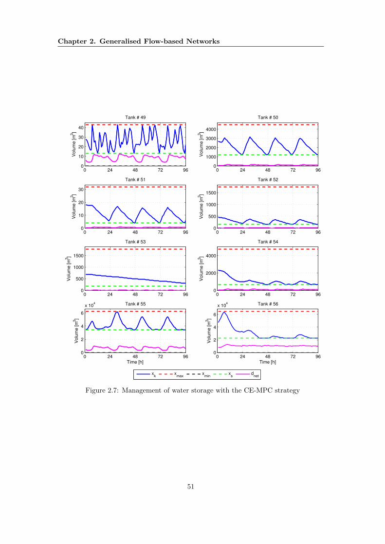
Chapter 2. Generalised Flow-based Networks
0 24 48 72 960
10
20
30
40
Tank # 49
Vo
lum
e [
m3]
0 24 48 72 960
1000
2000
3000
4000
Tank # 50
Vo
lum
e [
m3]
0 24 48 72 960
10
20
30
Tank # 51
Vo
lum
e [
m3]
0 24 48 72 960
500
1000
1500
Tank # 52
Vo
lum
e [
m3]
0 24 48 72 960
500
1000
1500
Tank # 53
Vo
lum
e [
m3]
0 24 48 72 960
2000
4000
Tank # 54
Vo
lum
e [
m3]
0 24 48 72 960
2
4
6
x 104 Tank # 55
Vo
lum
e [
m3]
Time [h]
0 24 48 72 960
2
4
6
x 104 Tank # 56
Vo
lum
e [
m3]
Time [h]
xk
xmax
xmin
xs
dnet
Figure 2.7: Management of water storage with the CE-MPC strategy
51

Chapter 2. Generalised Flow-based Networks
0 24 48 72 960
1
2
Flo
w [
m3/h
]
Actuator # 48
0 24 48 72 96−2
−1
0
1
2
0 24 48 72 960
0.5
1
Flo
w [
m3/h
]
Actuator # 49
0 24 48 72 96−2
0
2
0 24 48 72 960
0.5
Flo
w [
m3/h
]
Actuator # 71
0 24 48 72 960
0.01
0.02
0 24 48 72 960
0.5
Flo
w [
m3/h
]
Actuator # 110
0 24 48 72 96−1
0
1
0 24 48 72 96
0
Flo
w [
m3/h
]
Actuator # 81
0 24 48 72 96−1
0
1
0 24 48 72 960
1
2
3
Flo
w [
m3/h
]
Actuator # 83
0 24 48 72 96−1
−0.5
0
0.5
1
0 24 48 72 960
0.5
1
1.5
2
Time [h]
Flo
w [
m3/h
]
Actuator # 84
0 24 48 72 96−1
−0.5
0
0.5
1
0 24 48 72 960
0.5
Time [h]
Flo
w [
m3/h
]
Actuator # 87
0 24 48 72 960
0.05
uk
umax
umin Electric tariff pattern
Figure 2.8: Optimal operation of a sample of actuators in the Barcelona DWN
52

Part II
Centralised MPC Schemes forEconomic and Robust Operation
53


Chapter 3
Economic MPC Strategies forGeneralised Flow-based Networks
This chapter addresses the management of generalised flow-based networks regarding a
multi-objective cost function by means of economically-oriented MPC strategies. Here, it
is shown that the economic MPC framework is flexible to enhance the dynamic minimum
cost flow scheduling problem by guaranteeing recursive feasibility, asymptotic economic
performance and possibly asymptotic stability, even under changes of the economic cost
function. The chapter focuses on the design of economic predictive controllers for net-
works with periodically-time varying operation.
3.1 Introduction
Recalling the discussion in § 1.2.4, the predominant approach to incorporate economic
information in control applications is to consider a hierarchical control structure, where
standard MPC controllers are designed for tracking economic operational set-points that
are computed usually in an upper layer by means of a real-time optimiser (RTO) or a
steady-state target optimiser (SSTO), which usually use complex non-linear stationary
models and larger sampling times than the regulatory MPC layer. A more appealing al-
ternative from an economic point of view is to formulate a predictive controller that uses
a simplified control-oriented model and integrates the economic and control objectives
in a single optimisation problem, as has been introduced in § 2.3.2 for re-scheduling of
dynamic network flows. Nevertheless, the main drawback of these aforementioned alter-
55

Chapter 3. Economic MPC Strategies for Generalised Flow-basedNetworks
natives is the lack of mechanisms to retain feasibility of the MPC optimisation problem
at each time step (even under nominal conditions). This feasibility loss could be caused
due to different reasons, e.g., the time-varying nature of disturbances and parameters,
the time-scale differences and model mismatch in the hierarchical architecture, the omis-
sion of long-term effects of demands within the finite horizon scheduling problem, among
others.
In order to tackle the aforementioned feasibility problem without softening the orig-
inal constraints, additional ingredients are often included in the standard MPC for-
mulation, specifically, terminal constraints and/or terminal penalties [112]. The use of
economic cost functions directly in the MPC setting has lead to the so-called economic
MPC framework, and several formulations exists [53], where recursive feasibility, closed-
loop stability and/or average asymptotic performance can be guaranteed under some
form of dissipativity, duality or convexity assumptions.
This chapter is particularly focused on the periodic operation of generalised flow-
based networks. Five different MPC formulations are discussed: a hierarchical two-layer
approach, an economic MPC with periodic terminal equality constraint, an economic
MPC with periodic terminal penalty and terminal region, and two different modifications
of the terminal equality constraint based formulation, which are meant to overcome
possible feasibility losses in the presence of changing operating patterns. The discussed
schemes are tested and compared by means of the Barcelona’s drinking water network
case study, specifically using the sector model (see Figure 2.5).
3.2 Problem Statement
Consider a generalised flow-based network being described in the form (2.10), satisfying
Assumptions 2.6 and 2.7 and with states and controlled flows constrained to lie in the
convex and compact sets X and U defined in (2.11). The basic problem considered in this
section is that of finding conditions under which (2.14) is solvable at time step k ∈ Z+,
and conditions under which feasibility at k implies feasibility for all subsequent time
steps t > k, i.e., recursive feasibility. Here, Assumption 2.9 is dropped, and the control
synthesis problem is considered under the following interpretation (similar to [146]):
56

Chapter 3. Economic MPC Strategies for Generalised Flow-basedNetworks
Interpretation 3.1 (Sup-Inf Type Information). At any time step k ∈ Z+ when thedecision concerning the controlled flow uk is taken, both the state xk and the demand(uncontrolled flow) dk ∈ Dk := d ∈ Rp | 0 ≤ d ≤ dmax,k, dmax,k ∈ Rp+ are known, whilefuture demands dk+i are unknown for all i ∈ Z+ and can take arbitrary values dk+i ∈Dk+i, i ∈ Z+. The controller has also knowledge of the sequence of sets Dk+ii∈Z[1,N−1]
for a given horizon N ∈ Z+.
The above interpretation can be considered as a non-cooperative two-player dynamic
game that leads to a max-min optimal control problem, whose treatment in the robust
MPC literature is quite narrow; see [146] and references therein. In this game, the
first player is the controller, which has access to the current state xk and the current
demand dk when determining the controlled flow uk at each time step k. Specifically,
the controller employs a control law κN : Z+ ×Rn ×Rp → Rm to set a control action of
the form
uk = κN (k, xk, dk). (3.1)
The second player, often called the adversary, is the entity (e.g., the customer) which
demands a flow of commodity without having information about the state of the system
nor the controller. At each time step k, the adversary employs a policy δ : Z+ → Rp to
determine exogenously the demand, i.e., dk = δ(k) ∈ Dk.
To characterise the set of initial states and the admissible feedback control law (3.1)
for which (2.14) is solvable at time step k = 0 under Interpretation 3.1, some additional
notation is introduced. Let φ(i;xk,uk,dk) denote the solution of the dynamic state
update equation (2.10a) at the time step i ∈ Z+, starting from the state xk and reached
under the control sequence uk and the demand sequence dk. In addition, define the
following set:
V(d) := u ∈ Rm | Euu+ Edd = 0, d ∈ D, (3.2)
U(d) := U ∩ V(d), (3.3)
where V(d) is the set of control actions that satisfy the mass balance at static nodes for
a given demand d ∈ D. Likewise, some useful definitions are recalled below.
Definition 3.1 (Admissible uk and dk). Given the state xk and a target state set T, thecontrol sequence uk = uk+i|ki∈Z[0,N−1]
and the demand sequence dk = dk+ii∈Z[0,N−1]
are admissible if
57

Chapter 3. Economic MPC Strategies for Generalised Flow-basedNetworks
(i) dk+i ∈ Dk+i, ∀i ∈ Z[0,N−1],
(ii) for all dk ∈ Dk × Dk+1 . . .× Dk+N−1, it holds that
(φ(i;xk,uk,dk), uk+i|k(xk,dk)) ∈ X× U(dk+i), ∀i ∈ Z[0,N−1], and
φ(N ;xk,uk,dk) ∈ T.
Definition 3.2 (N -step max-min controllability). Let DN,k be the set of all admissibledemand sequences dk and UN (xk,dk) the set of all admissible control sequences uk attime step k ∈ Z+ for given time-horizon N > k. A state xk ∈ X is N -step max-mincontrollable to a target set T ⊆ X if and only if for all admissible demand sequences dkthere exists an admissible control sequence, i.e., UN (xk,dk) 6= ∅. A set XN is called N -step max-min controllable if all xk ∈ XN are N -step max-min controllable to the targetset.
An important ingredient in the N -step max-min controllability is the one-step con-
trollable set, which for a generalised flow-based network under Interpretation 3.1 is given
by the pre-image mapping
B(X,D) := x ∈ X | ∀d ∈ D, ∃u ∈ U(d) such that Ax+Bu+Bdd ∈ X, (3.4)
where X and D are a one-step target set of states and a set of demands, respectively.
Therefore, by inspection of Definition 3.2, at k = 0, the i-step max-min controllable sets,
with i ∈ Z[0,N ], are given by iteration of the mapping B(·, ·), i.e.,
Xi = B(Xi−1,DN−i), i ∈ Z[1,N ], (3.5)
with the boundary condition X0 := T ⊆ X. Each controllable set has an associated
max-min set-valued control map given for all i ∈ Z[1,N ] by:
Ui(x, d) := u ∈ U | ∀(x, d) ∈ Xi×DN−i, Euu+Edd = 0 , Ax+Bu+Bdd ∈ Xi−1. (3.6)
Therefore, the set of all admissible control sequences u = uii∈Z[0,N−1]is defined as
UN (x,d) := u | ui ∈ U, ∀i ∈ Z[0,N−1] and ∀(x, d) ∈ XN−i × Di,
Euui + Edd = 0 , Ax+Bu+Bdd ∈ XN−i−1.(3.7)
As shown in [146], from continuity of the system dynamics and compactness of X, Uand Di, if the target set is compact, then the i-step max-min controllable sets and their
corresponding set-valued control maps are compact (possibly empty).
58

Chapter 3. Economic MPC Strategies for Generalised Flow-basedNetworks
3.3 Existence of Admissible Controlled Flows
Showing the resolvability of (2.14) requires first the existence of an admissible control
sequence satisfying Definition 3.1. This involves establishing the N -step controllability
of the constrained generalised flow-based network following Definition 3.2 with target
set T = X. The following basic result is the starting point for the feasibility analysis.
Proposition 3.1. The N -horizon scheduling-control problem (2.14) is solvable at giveninitial time step k ∈ Z+ if and only if the N -step max-min controllable set is non-empty, i.e., XN 6= ∅ and the state xk belongs to any of the one-step controllable sets Xj,j ∈ Z[0,N ]. In such a case, a control sequence exists satisfying uk ∈ UN (x,d).
Proof : The statement follows directly from Definitions 3.1 and 3.2.
It is important to remark that Proposition 3.1 only ensures feasibility of the MPC
optimisation problem (2.14) at time step k, but not at future steps t > k. Therefore, it is
desired to find conditions under which recursive feasibility of the optimisation problem
is guaranteed for any sequence of admissible demand flows. In order to do so, something
has to be assumed regarding the limit behaviour of the sequence of demand time-varying
sets Dkk∈Z[0,∞). A suitable assumption is that this sequence of sets is asymptotically
convergent either to a single invariant set or to a limit-cycle of sets. For brevity of the
exposition, this chapter considers the first case.
Assumption 3.1. Dk → D := d ∈ Rp | 0 ≤ d ≤ dmax, dmax ∈ Rp+ as k → ∞, withDk ⊆ D,∀k ∈ Z+.
Establishing initial conditions that guarantee the existence of admissible control se-
quences for all time steps requires the following set invariance notions.
Definition 3.3 (Max-min robust control invariance). A set C ⊆ X is a max-min robustcontrol invariant set for the system (2.10) with x ∈ X, u ∈ U and d ∈ D if and onlyif C ⊆ B(C, D), i.e., for all (x, d) ∈ C × D there exists a control u ∈ U such thatAx+Bu+Bdd ∈ C and Euu+ Edd = 0.
Definition 3.4 (Maximal max-min robust control invariant set). A max-min robustcontrol invariant set is called the maximal max-min robust control invariant set (heredenoted as C∞) if and only if it contains all max-min robust control invariant sets.
Remark 3.1. The set C∞ is unique (possibly empty). Consider the sequence of max-min controllable sets Xii∈Z[0,∞)
generated by (3.5) with N → ∞. If Assumption 3.1
holds then the sequence Xii∈Z[0,∞)converges to the set X :=
⋂∞i=0 Xi. Moreover, from
59

Chapter 3. Economic MPC Strategies for Generalised Flow-basedNetworks
Definition 3.3, an i-step controllable set Xi is max-min robust control invariant if andonly if Xi ⊆ Xi+1 = B(Xi, D). In addition, for the target set T = X, the maximal max-min robust control invariant set satisfies C∞ ⊆
⋂∞i=0 Xi and it is finitely determined,
with C∞ = Xi, if and only if Xi = B(Xi, D) for some i ∈ Z+. The limit behaviour of themax-min controllable sets leads to the result in Proposition 3.2. ♦
Proposition 3.2. The MPC problem (2.14) is solvable at any time step k ∈ Z+ if andonly if the maximal max-min controllable set is non-empty, i.e., C∞ 6= ∅, and the statexk belongs to it. In such a case, a control sequence exists satisfying
uk ∈ U∞(xk,dk) = u = uii∈Z[0,N−1]∈ UN | ∀dk = dk+ii∈Z[0,N−1]
∈ DN ,
φ(i;xk,u,dk) ∈ C∞ and Euui + Eddk+i = 0 , ∀i ∈ Z[0,N−1].(3.8)
Proof : The statement follows directly from Definitions 3.3 and 3.4.
Remark 3.2. For large-scale systems with more complex constraint sets, the compu-tation of the maximal max-min robust control invariant set C∞ might be challenging.Constructing any non-empty robust control invariant set Ω ⊆ X could be a simpler ap-proach. From Definition 3.3, for k = 0, all x0 ∈ Ω are controllable. Since Ω is controlinvariant, it follows that Ω ⊆ XN ⊆ C∞. Hence, the non-emptiness condition C∞ 6= ∅holds by construction and a control sequence exists for any time step. ♦
Theorem 3.1. Let Assumptions 2.5, 2.6 and 3.1 hold. Then, under Interpretation 3.1,there exists an admissible max-min feedback control strategy of the form (3.1) such thatfor all dk ∈ D and all k ∈ Z+, a generalised flow-based network satisfies flow conservationconstraints (2.10) and capacity constraints (2.11), if and only if the following conditionsare satisfied:
BdD ⊆ −BU, (3.9a)
EdD ⊆ −EuU. (3.9b)
Moreover, the largest admissible initial set X0 ⊆ X, for which the MPC algorithm remainsfeasible for all time and all (x, d) ∈ X0×D, is non-empty and given by the maximal max-min robust control invariant set, i.e., X0 = C∞ 6= ∅, which is explicitly characterised andgiven by
C∞ = B(X, D) =((X⊕ (−BU))BdD
)∩ X. (3.10)
Proof: Conditions in (3.9) can be considered as matching conditions for robust control
system design, see [187] and references therein. Condition (3.9a) has been previously used
under a min-max framework in [22, 23] and proved to be one of the required ingredients
to ensure the existence of a min-max winning strategy in a dynamic LTI system. For
generalised flow-based networks, it is necessary, in addition, to include condition (3.9b).
60

Chapter 3. Economic MPC Strategies for Generalised Flow-basedNetworks
Both matching conditions are necessary and sufficient under Interpretation 3.1. The
proof follows the line of arguments in [23], and is detailed here for completeness. For
necessity, let d∗ ∈ D be a suitable demand flow such that Bdd∗ /∈ −BU, i.e., there exists
a hyperplane in Rn such that
∃z1 ∈ Rn, ε > 0, z>1 Bdd∗ ≥ −z>1 Bu+ ε1, ∀u ∈ U. (3.11)
Then, for any x0 ∈ X and selecting dk = d∗ for all k ≥ 0, from (2.10a) it is obtained
that xk = Ax0 +∑k−1
i=0 (Bui +Bdd∗) for any feasible sequence ui ∈ Uk−1
i=0 . Multiplying
both sides of this latter equality by z>1 , it follows from (3.11) that
z>1 xk = z>1 Ax0 + z>1
k−1∑i=0
(Bui +Bdd∗) ≥ z>1 x0 + ε1k,
which implies that for k sufficiently large, xk /∈ X. In the same way, assume that there
exists a vector z2 6= 0 in Rq that strongly separates EuU from −Edd∗. Then, there
exists a ε2 ≥ 0 such that z>2 Edd∗ ≥ −z>2 Euu + ε2 for every u ∈ U. This latter implies
the violation of the flow conservation in (2.10b). Therefore, both (3.9a) and (3.9b)
are necessary conditions to guarantee the possibility for the controller to find admissible
flows that counteract the effect of any demand and to keep the states within their feasible
domain.
Conditions in (3.9) are also sufficient. First, it follows from (3.9a) and from the
Minkowski sum properties, that (X⊕ (−BU))BdD ⊇ X, which implies that the set C∞
defined in (3.10) is not empty. Now, from Definitions 3.3 and 3.4, for each xk ∈ C∞ 6= ∅and all dk ∈ D, with k = 0, there exists a uk ∈ U such that xk+1 = Axk +Buk +Bddk ∈C∞ and Euuk + Eddk = 0. By (3.9a) and (3.9b), for each dk ∈ D, there exists a uk ∈ Usuch that Buk = −Bddk and Euuk = −Eddk. Therefore, xk+1 ∈ X. By repeating the
same argument for all subsequent k ∈ Z[1,∞), it can be shown that all the states x ∈ C∞
define admissible initial conditions to keep future state trajectories feasible for all time
steps.
Now, to prove that C∞ = B(X, D), recall the recursion (3.5). Assume that the one-
step controllable set X1 = B(X0, D) 6= ∅ with X0 = X and D = D. From the definition
of the pre-image map B(·, ·) in (3.4), it follows that
X1 = x ∈ X | ∀d ∈ D, ∃u ∈ U, such that Ax+Bu+Bdd ∈ X, Euu+Edd = 0. (3.12)
61

Chapter 3. Economic MPC Strategies for Generalised Flow-basedNetworks
In order to find an explicit characterisation of the set X1, it is needed to eliminate the
quantifiers in (3.12) and obtain a single equation. To do so, one can first eliminate the
algebraic constraint (Euu + Edd = 0) by using a suitable parametrisation of u. From
Assumption 2.5, the following parametrisation can be performed:
∀w ∈ D, ∃v, such that u = P
[ −M1
I(m−q)
]︸ ︷︷ ︸
Q
v + P
[−Ed0p
]︸ ︷︷ ︸
R
d ∈ U, (3.13)
where v ∈ Rm−q is a reordered subset of the control inputs, P ∈ Rm×m is a positive
permutation matrix, I(m−q) is an (m − q)-square identity matrix, 0p is a p-square null
matrix and M1 ∈ Rq×(m−q) is a matrix resultant from the rearrangement of the elements
of u in the permutation process. For further details refer to Appendix B. Replacing
(3.13) in (3.12) leads to
B(X, D) = x ∈ X | ∀d ∈ D, ∃v ∈ Rm−q, such that Qv +Rd ∈ U, and
Ax+B(Qv +Rd) +Bdd ∈ X.(3.14)
Eliminating the quantifiers in (3.14), yields
X1 =((X⊕ (−BU))BdD
)∩ X. (3.15)
Similarly, it can be verified that X2 = B(X1, D) is given explicitly by
X2 =((X1 ⊕ (−BU))BdD
)∩ X
=((((
(X⊕ (−BU))BdD)∩ X
)⊕ (−BU)
)BdD
)∩ X. (3.16)
From Minkowski sum properties, it can be verified that (X⊕ (−BU)) BdD ⊇ X if
(3.9a) holds. Therefore, it holds that
X2 =((X⊕ (−BU))BdD
)∩ X = X1.
Hence, from Remark 3.1, the maximal max-min robust control invariant set1 is finitely
determined and given by the fixed point of the pre-image mapping, i.e.,
C∞ =((X⊕ (−BU))BdD
)∩ X,
which concludes the proof.
1Notice that even when the explicit expression of C∞ results to be the same as if considering only
(2.10a) for the dynamic nodes, the static balance in (2.10b) requires the extra condition (3.9b) toguarantee C∞ 6= ∅.
62

Chapter 3. Economic MPC Strategies for Generalised Flow-basedNetworks
3.4 Synthesis of Flow-based Controllers
Initial conditions under which the MPC problem (2.14) ensures feasibility for all time
steps has been discussed in the previous section. Nevertheless, in several applications
of generalised-flow based networks, properties such as asymptotic average performance
or convergence to some economically optimal set-point or periodic trajectory may in
addition be required. Therefore, this section presents the design of different economic
MPC controllers, which are specialised for the case when the network is operating under
periodically time-varying demands and costs. Such periodic operation results to be of
interest for the management of critical infrastructures such as water supply networks,
energy distribution networks, supply-chains, among others, where the flow costs and
demands often follow a periodic pattern.
3.4.1 Economic Scheduling Optimisation for Periodic Operation
A special case of the control synthesis problem is when the demand schedule is a periodic
flow that is known a priori. In such a case, the time-varying demand sets Dk defined
in the previous section become periodically time-varying singletons. Other particularity
shared in several networks is to operate under periodically time-varying costs, which are
usually defined by a time-of-use pricing scheme. Hence, the following assumptions are
in order.
Assumption 3.2. The demand dk = δ(k) ∈ Dk is perfectly known and follows a nominalT -periodic pattern. Hence, Dk = δ(k) for all k ∈ Z+, with the consumer policy δsatisfying δ(k) = δ(k + T ) and consequently dk = dk+T for all k. The smallest integerT ∈ Z≥1 fulfilling this latter equality is called the period of the uncontrolled flows.
Assumption 3.3. The system operates minimising a T -periodic economic stage cost` : Z+ × Rn × Rm → R+, which satisfies `(k, x, u) = `(k + T, x, u), T ∈ Z≥1, for all k.This stage cost is continuous.
In view of Assumptions 3.2 and 3.3, an economically optimal flow scheduling can be
computed by solving the following T -horizon optimisation problem PT (k, dT ,pT ):
V 0T (k, dT ,pT ) = min
x0,uVT (k, x0, u) :=
T−1∑i=0
`(k + i, xi, ui) (3.17)
subject to (x0, u) ∈ FT (dT ),
63

Chapter 3. Economic MPC Strategies for Generalised Flow-basedNetworks
with the set FT (dT ) being compact and defined as
FT (dT ) := (x0, u) | u = uii∈Z[0,N−1]∈ UNr , φ(i; x0, u, dT ) ∈ Xr, φ(N ; x0, u, dT ) = x0,
Euui + Eddbk+icT = 0, i ∈ Z[0,N−1],(3.18)
where dT := dbk+icT i∈Z[0,T−1]and pT := pbk+icT i∈Z[0,T−1]
denote respectively the
nominal periodic demand and the vector of economic parameters defining the T -periodic
stage cost function `(k + i, ·, ·), k ∈ Z+. The sets Xr and Ur are closed hyperboxes
contained in the relative interior of the original constraint sets in order to avoid that
X and U are not active at the optimal trajectory. Assume that FT (dT ) 6= ∅, then the
minimum of (3.17) exists from compactness of FT (dT ) and continuity of `(i, ·, ·) for all
i. Moreover, from optimality and periodicity V 0T (0, dT ,pT ) = V 0
T (k, dT ,pT ) for all k.
The optimal state and input trajectories can be constructed from the solution of (3.17)
and given by x? = x?i = φ(i; x?0, u?, dT )i∈Z[0,T−1]
and u? = u?i i∈Z[0,T−1], respectively,
where φ(i; x?0, u?, dT ), denotes the i-step evolution of the dynamic state vector starting
from the initial condition x?0. In addition, it is possible to build the best T -periodic orbit
for system (2.10) as follows:
XT (dT ,pT ) :=T−1⋃i=0
x?i . (3.19)
In general, `(k + i, ·, ·), i ∈ Z[0,T−1], need not be positive definite with respect to any
setpoint and there does not necessarily exist a unique optimal feasible solution (x?, u?)
or unique orbit set XT (dT ,pT ). Hence, in the following one of the feasible solutions can
be arbitrarily selected or the cost function can be regularised to obtain a unique optimal
solution.
3.4.2 Nominal Economic MPC Strategies for Periodic Network Flows
In this section, different economically-oriented MPC strategies are stated for the gener-
alised flow-based networks scheduling-control problem. These schemes are: a two-layer
architecture where an economic planner and a tracking MPC are interacting, a stan-
dard economic MPC with terminal state constraint, and two one-layer economic MPC
strategies that account for changes in the economic criteria.
64

Chapter 3. Economic MPC Strategies for Generalised Flow-basedNetworks
Hierarchical MPC
This is a two-layer optimal controller, where a separation of objectives, models and/or
time-scales may be performed. Below, the optimisation problems involved in this hier-
archical approach are stated.
Upper layer Economic MPC. In this layer, a dynamic real-time optimiser (D-RTO)
computes the optimal time-varying state and input T -periodic trajectories by solving
problem PT (k, dT ,pT ) at the beginning of each operating cycle. Denote with (x?z, u?z)
the optimal solution of (3.17) at time step z ∈ Z+, then these economically optimal
trajectories govern a lower layer MPC described below.
Lower layer Tracking MPC. In this layer, conventional MPC is used to enforce the system
to track the pre-computed optimal trajectories. The associated optimisation problem is
stated as
minuk
Hlp−1∑i=0
‖xk+i|k − x?bk+icT |z‖2Qx
+ ‖uk+i|k − u?bk+icT |z‖2Qu, (3.20a)
subject to:
xk+i+1|k = Axk+i|k +Buk+i|k +Bddbk+icT , ∀i ∈ Z[0,H
lp−1]
(3.20b)
Euuk+i|k + Eddbk+icT = 0, ∀i ∈ Z[0,H
lp−1]
(3.20c)
xk+i|k ∈ X, ∀i ∈ Z[1,H
lp−1]
(3.20d)
uk+i|k ∈ U, ∀i ∈ Z[0,H
lp−1]
(3.20e)
xk+H
lp|k
= x?k+H
lp|z, (3.20f)
xk|k = xk, (3.20g)
where H lp ∈ Z≥1 is the prediction horizon of the lower layer, xk ∈ Rn is the measured
initial state at time step k ∈ Z+, the weighting matrices satisfy Qx 0, Qu 0 and
bk + icT denotes the modulus operation mod(k + i, T ). Following the receding horizon
technique, the control law derived under this hierarchical scheme is given by κ(xk, dT
)=
u?k|k, i.e., only the first control action of the optimal input sequence obtained in (3.20) is
applied to the system. If asymptotic convergence to the upper layer trajectory is desired,
the tracking problem can be reformulated in terms of the error ek+i = xk+i|k− x?bk+icT |z,
leading to a set-point (origin) stabilization problem of the error dynamics; see e.g., [56].
65

Chapter 3. Economic MPC Strategies for Generalised Flow-basedNetworks
Note that the upper layer may have an equal or larger sampling time than the one of
the lower layer, i.e., ∆t1 ≥ ∆t2. The main drawback of this two-layer MPC approach for
the management of generalised flow-based networks is that if the economic parameters
of the cost function or the demand patterns change in time with a high rate, then the
transitory periods will be so that the interaction between layers could lead to a possible
loss of feasibility or to an economic performance degradation.
Standard Economic MPC
The main feature of this approach, in contrast with the hierarchical scheme even when the
two-layers may work with the same sampling time, is that the standard economic MPC
considers the global economic criteria directly as the stage cost of the MPC controller
and avoids penalising the tracking error with respect to the targets [150]. The associated
FHOP for the periodic operation of the system is stated as
minuk
VN (k, xk,uk) =N−1∑i=0
`(k + i, xk+i|k, uk+i|k), (3.21a)
subject to:
xk+i+1|k = Axk+i|k +Buk+i|k +Bddbk+icT , ∀i ∈ Z[0,N−1] (3.21b)
Euuk+i|k + Eddbk+icT = 0, ∀i ∈ Z[0,N−1] (3.21c)
xk+i|k ∈ X, ∀i ∈ Z[1,N−1] (3.21d)
uk+i|k ∈ U, ∀i ∈ Z[0,N−1] (3.21e)
xk+N |k = x?bk+NcT , (3.21f)
xk|k = xk, (3.21g)
where xk is the measured initial state at time step k ∈ Z+, and x?bk+NcT is the optimal
periodic value obtained in (3.17) that corresponds to the time step k. Similarly to
conventional tracking MPC, the first optimal control action u?k|k obtained from (3.21) is
applied to the system. As shown in [7, Theorem 4], standard economic MPC is capable
of enhancing the closed-loop economic performance of the system if this is not optimally
operated at steady state, achieving an asymptotic average cost that is at least as good
as the average cost of the best periodic trajectory obtained in (3.17), i.e.,
lim supM→+∞
∑Mk=0 `(k, xk, uk)
M + 1≤∑T−1
k=0 `(k, x?k, u
?k)
T. (3.22)
66

Chapter 3. Economic MPC Strategies for Generalised Flow-basedNetworks
For a general (possibly non-convex) cost functional `(k, x, u), the standard economic
MPC may not be a stabilising controller. In fact, to guarantee stability and optimal
steady-state operation of a system, certain dissipativity conditions must be satisfied
(see [117] and references therein). For the particular case of periodic operation, different
periodic dissipativity notions were introduced in [75], from where the following definition
is extracted (adapted to our setting).
Definition 3.5. Let Assumptions 3.2 and 3.3 hold. Then, system (2.10) is called strictlydissipative with respect to a T -periodic supply rate s : Z[0,T−1] × X × U → R, if thereexists a T -periodic storage function λ : Z[0,T−1] × X→ R, and a function ρ ∈ K∞, suchthat the following inequality holds for all (k, x, u) ∈ Z[0,T−1] × X× U(dk):
s(k, x, u) + λ(k, x)− λ(k + 1, Ax+Bu+Bddk) ≥ ρ(‖x− x?k‖). (3.23)
Therefore, in order to enforce convergence to the optimal trajectory (x?, u?), the follow-
ing is assumed.
Assumption 3.4. System (2.10) is strictly dissipative with respect to the supply ratedefined as s(k, x, u) = `(k, x, u)− `(k, x?k, u?k).
There exist methods to determine storage functions λ that satisfy Assumption 3.4
for linear systems with convex constraints and convex cost functions, see e.g., [45, 48]
for time-invariant systems and [194] for periodically time-varying systems.
Nominal asymptotic stability of the closed-loop system operating with periodic de-
mand and periodic cost is guaranteed by problem (3.21) and can be proved directly
from [194, Theorem 1] under certain additional assumptions, i.e., (weak) controllability
of system (2.10) and strong duality of problem (3.17), and with minor modifications to
include the algebraic equation (2.10b). Adapting [7, Definition 6.1] to the periodic case,
it can be said that when the system is forced to optimally operate at the best periodic
trajectory (x?, u?), its asymptotic average performance is under-bounded by
lim supM→+∞
∑Mk=0 `(k, xk, uk)
M + 1≥∑T−1
k=0 `(k, x?k, u
?k)
T. (3.24)
If the above inequality is strict (>), then the system is sub-optimally operated off its
best periodic trajectory.
Even when the economic MPC controller improves the asymptotic average economic
performance of the system when not enforcing convergence, its main weakness is a pos-
sible loss of feasibility due to changes in the periodic demand pattern or in the economic
67

Chapter 3. Economic MPC Strategies for Generalised Flow-basedNetworks
parameters affecting the cost function, which make the previous target state to be pos-
sibly unreachable under the given prediction horizon. Consequently, the standard eco-
nomic MPC controller still depends on the pre-computed optimal T -periodic trajectory,
which should be computed when detecting demand or costs changes before the MPC
runs in order to obtain compatible terminal states.
Economic MPC for Changing Operating Patterns
In order to overcome the possible loss of feasibility due to changing operating patterns
caused by the parameters of the cost function or by the demands, two approaches follow-
ing the ideas in [82] and [106] are proposed here to be solved in a one-layer architecture.
These schemes integrate in different ways the optimal trajectory problem (3.17) with
the standard economic MPC in (3.21).
Option A: Enlargement of the prediction horizon
minuk
N+T−1∑i=0
`(k + i, xk+i|k, uk+i|k), (3.25a)
subject to:
xk+i+1|k = Axk+i|k +Buk+i|k +Bddbk+icT , ∀i ∈ Z[0,N+T−1] (3.25b)
Euuk+i|k + Eddbk+icT = 0, ∀i ∈ Z[0,N+T−1] (3.25c)
xk+i|k ∈ X, ∀i ∈ Z[1,N+T−1] (3.25d)
uk+i|k ∈ U, ∀i ∈ Z[0,N+T−1] (3.25e)
xk+N+T |k = xk+N |k (3.25f)
xk|k = xk, (3.25g)
where T ∈ Z+ is the period of the demands and N = cT with c ∈ Z+. Note that in this
option, slight changes of the economic MPC framework are required. First, the terminal
constraint (3.21f) is replaced with (3.25f). Second, the prediction horizon is extended to
cover the period of the cost and process dynamics. This is done in order to avoid the use
of a precomputed trajectory. Note that (3.21f) is a sort of generalised terminal constraint
associated to a periodic trajectory that results from the same prediction model used in
problem rather than to a precomputed trajectory. This makes the system find its own
new optimal orbit if the operational conditions (prices or demands) change.
68

Chapter 3. Economic MPC Strategies for Generalised Flow-basedNetworks
Option B: Inclusion of a pseudo-reference to track
minukx
s0,u
sk
T−1∑j=0
γE `(k + j, xsj , usj) +
N−1∑i=0
γT
(‖xk+i|k − xsi‖2Qx
+ ‖uk+i|k − usi‖2Qu
),
(3.26a)
subject to (3.21b)-(3.21e) ∀i ∈ Z[0,N ] and
xsj+1 = Axsj +Busj +Bddbk+jcT , ∀j ∈ Z[0,T−1] (3.26b)
Euusj + Eddbk+jcT = 0, ∀j ∈ Z[0,T−1] (3.26c)
(xsj , usj) ∈ Xr × Ur, ∀j ∈ Z[0,T−1] (3.26d)
xsT = xs0, (3.26e)
xk+N |k = xsN , (3.26f)
xk|k = xk, (3.26g)
with Qx 0, Qu 0 and the prediction horizon N selected in such a way that N ≤ T ,
being T ∈ Z≥1 the period of the time-varying parameters. Moreover, γE ∈ R+ and
γT ∈ R+ are scalars introduced to establish a trade-off between economic and tracking
performance. Recall that Xr and Ur are tightened constraint sets that are used here
to avoid active constraints at the optimal pseudo-reference. Note that the constraints
(3.26b)-(3.26e) imposed on the pseudo-reference model are identical to the constraints
of periodic scheduling problem (3.17), and guarantee that this trajectory is admissible
and periodic. The terminal constraint (3.26f) forces the predicted trajectory of the real
system to reach the pseudo-reference in N steps.
This controller has the following interesting theoretical and practical properties that
are proved and discussed in detail in [106]:
(i) The controller guarantees convergence of the closed-loop system to the optimal
trajectory (x?, u?) without requiring its a priori computation by a dynamic RTO
for the given periodic economic parameters.
(ii) The proposed optimisation problem is recursively feasible for the nominal periodic
demand, even if the economic cost function changes.
(iii) The domain of attraction of the proposed controller is in general larger than the
domain associated with the standard economic MPC approach.
69

Chapter 3. Economic MPC Strategies for Generalised Flow-basedNetworks
(iv) The closed-loop system is input-to-state stable with respect to additive distur-
bances, whenever the evolution of the system is admissible. This implies that the
closed-loop system is robust to small variations of the demand vector d.
Remark 3.3. The economic MPC controllers associated with the optimisation problems(3.4.2) and (3.26) are not enforcing convergence to the precomputed optimal trajectoryobtained in (3.17). Instead, they are meant to retain feasibility under possible changes ofthe economic parameters in the cost function and to find new optimal stable trajectoriesfor the current conditions. To do so, certain assumptions are still required such as (weak)controllability and (strict) convexity of the cost function.
3.4.3 Numerical Results
This section presents the results of applying the economic MPC approaches described in
§ 3.4.2 to the small-size sector example (see Figure 2.5) of the drinking water network case
study described in § 2.4. The FHOP of each strategy is properly adapted to incorporate
the additional safety constraint and slack variables used in (2.23). The sampling time
is ∆t = 3600 s. The simulation horizon is sixteen days (Ns = 384 hours) for each
strategy. The weights of the aggregate user-defined cost function are γ1 = 100, γ2 = 1,
and γ3 = 10. For the tracking terms, the weighting matrices Qx and Qu are set up
arbitrarily as identity matrices of proper dimensions (although other weights can be
freely use depending on the desired response). The prediction horizon has been selected
as N = 24 hours due to the periodicity of both water demands and electricity prices
(i.e., T = 24 hours). For the hierarchical controller, the upper layer is executed every
24 hours as usually done in water distribution scheduling, while the lower layer runs
in an hourly basis as in the other economic MPC strategies. The initial common state
for all simulations is x0 = [160.44, 646.23, 633.89]> in m3 and the security threshold
is s = [42, 18.0, 270]> in m3. The formulation of the optimisation problems and the
closed-loop simulations have been carried out using YALMIP Toolbox, CPLEX solver
and Matlab R2012b (64 bits), running in a PC Intel Core E8600 at 3.33GHz with 8GB
of RAM.
The closed-loop performance of each controller has been assessed using the key per-
formance indicators (KPIs) described in § 2.4.4. Results are summarised in Table 3.1,
where the hierarchical MPC, the standard economic MPC, and both economic MPC
options A and B for changing patterns are compared and labeled HEMPC, EMPC,
70

Chapter 3. Economic MPC Strategies for Generalised Flow-basedNetworks
Table 3.1: Comparison of controller performance
Controller KPIE KPI∆U
(e.u.) (m3/s)2
Ideal scheduling (Problem (3.17)) 28.6056 2.06× 10⁻³
HEMPC(1) 28.4347 2.14× 10⁻³
HEMPC(2) 28.6114 2.08× 10⁻³
EMPC(1) 28.4124 8.89× 10⁻⁷
EMPC(2) 28.6080 8.89× 10⁻⁷
EMPCT-A(1) 28.4124 8.89× 10⁻⁷
EMPCT-A(2) 28.6041 8.89× 10⁻⁷
EMPCT-B(1)@γO=1, γT=1 28.5165 2.17× 10⁻³
EMPCT-B(1)@γO=1, γT=10 28.4493 2.35× 10⁻³
EMPCT-B(1)@γO=1, γT=100 28.4178 2.34× 10⁻³
EMPCT-B(1)@γO=10, γT=1 28.8128 2.29× 10⁻³
EMPCT-B(2)@γO=1, γT=100 28.6120 2.43× 10⁻³
e.u.: economic units.
Subindex (1) indicates non-periodic behaviour enforced while(2) indicates that the periodic constraint is enforced.
EMPCT-A and EMPCT-B, respectively. The sub-index (1) indicates that the controller
is not including the terminal constraint, while sub-index (2) indicates that the terminal
periodic constraint is enforced. The safety indicator has been omitted in Table 3.1 given
that, for all simulated scenarios and strategies, KPIS = 0, which means that all of the
MPC controllers decided not to use water from the safety stocks for the given periodic
demand. Note that for each strategy the enforcement of terminal constraints implies an
increment of the economic cost. This decrease in performance is the price for gaining in
stability.
Furthermore, Table 3.2 discloses details of the production and operational costs re-
lated to each strategy starting from a non-optimal state x0 = [92.45, 905.82, 504.14]> in
m3, and compares the daily average economic performance of the controllers enforcing
their corresponding periodic terminal constraints. For the standard EMPC(2), the ter-
minal constraint is set up in relation to a pre-calculated optimal cycle obtained from
71

Chapter 3. Economic MPC Strategies for Generalised Flow-basedNetworks
Table 3.2: Comparison of daily average costs of EMPC strategies
Controller Water Cost Electric Cost Daily Cost(e.u./day) (e.u./day) (e.u./day)
EMPC(2) 577.24 110.04 687.28
HEMPC(2) 610.02 134.13 744.15
EMPCT-A(2) 577.79 109.56 687.35
EMPCT-B(2) 577.75 109.79 687.54
e.u.: economic units
(3.17). In the HEMPC(2), the reference trajectory is computed by the upper layer every
24 hours. For controllers EMPCT-A(2) and EMPCT-B(2), no pre-calculated trajectory is
needed. It can be seen how the HEMPC(2) cost degrades notoriously the performance in
comparison with the other MPC strategies due to the time-scale separation in its layers.
Even when feasibility issues were not found for any of the strategies in this case study,
these results reaffirm the current tendency of improving the economic performance by
migrating to one-layer economic MPC controllers which are robust to changes in the
cost function.
To further highlight the performance of controllers EMPCT-A and EMPCT-B, which
cope with changing economic criterion, the price parameter of the economic term in
(2.22) has been affected switching the price profile at different time steps but keeping
the same period, see Figure 3.1. As it can be seen in Figure 3.2 for the evolution of
the states, both controllers maintain the recursive feasibility and stabilise at similar
trajectories.
Even so, the approach in (3.26), which includes a pseudo-reference and tracking
terms, presents a slightly higher cost with respect to the approach in (3.4.2). This
behaviour might be due to the regularisation terms that decrease the economic perfor-
mance if design parameters (i.e., γE , γT , Qx and Qu) are not properly tuned. A possible
enhancement could be to include the economic cost function also in the tracking term
of the EMPCT-B. Further simulations and numerical results of this latter controller for
this case study and for a four tank benchmark example can be found in [106].
72

Chapter 3. Economic MPC Strategies for Generalised Flow-basedNetworks
0 50 100 150 200 250 300 350 4000
0.05
0.1
u 4 cos
t [e.
u.]
0 50 100 150 200 250 300 350 4000
0.02
0.04
0.06
u 5 cos
t [e.
u.]
0 50 100 150 200 250 300 350 4000
0.2
0.4
u 6 cos
t [e.
u.]
Time [h]
Figure 3.1: Price-of-use for actuators u4, u5 and u6 in economic units (e.u.)
0 50 100 150 200 250 300 350 4000
500
1000
1500
2000
2500
3000
3500
Time [h]
Stat
es [m
3 ]
x1, EMPCT Ax2, EMPCT Ax3, EMPCT Ax1, EMPCT Bx2, EMPCT Bx3, EMPCT B
Figure 3.2: Evolution of some states under varying economic parameters
73

Chapter 3. Economic MPC Strategies for Generalised Flow-basedNetworks
3.5 Economic MPC for Periodic Systems
Previous stabilising strategies are based on a periodically time-varying terminal equality
constraint MPC formulation, in which the system is stabilised by forcing the termi-
nal state to a point of the best periodic orbit. Nevertheless, as highlighted in [6] for
the time-invariant case, a terminal equality constraint may result to be quite restric-
tive and should be removed or replaced with a terminal penalty and a terminal region
constraint. Therefore, the main contribution of this section is the extension and gen-
eralisation of previous results addressing periodic economic operation of time-invariant
systems with periodic costs to the case of periodically time-varying systems. Specifically,
a terminal penalty/region economic MPC formulation for general linear periodic systems
is proposed here. For this, the methodology proposed in [27], based on linear matrix
inequalities (LMIs), is incorporated into the economic MPC framework to design the
required periodically time-varying terminal penalty functions, terminal control laws and
terminal ellipsoidal regions. The resultant conditions are less conservative than those
of [194], thus leading to an improved size of the feasible set of initial conditions and a
possibly improved closed-loop performance.
Consider a class of dynamic time-varying affine system described by
xk+1 = f(k, xk, uk) := Akxk +Bkuk + wk, (3.27)
where xk ∈ Rn and uk ∈ Rm represent the system state and input vectors at current time
step k ∈ Z+, respectively. State measurements are assumed to be available at each time
step. The vector wk ∈W ⊆ Rp represents a known and bounded (possibly time-varying)
exogenous input. Matrices Ak and Bk are assumed to be known for each time step k.
The system is subject to (possibly time-varying) equality and inequality constraints
given in the form of a convex closed polyhedral set, which is defined as
Yk := (x, u) ∈ Rn+m | aj,kx+ bj,ku ≤ hj,k,∀j ∈ Z[1,r], ∀k ∈ Z+, (3.28)
where r ∈ Z≥1 is the number of hyperplanes and aj,k ∈ R1×n and bj,k ∈ R1×m for all
j ∈ Z[1,r] and k ∈ Z+. Denote by Xk ⊆ Rn and Uk ⊂ Rm the projections of Yk at each
time step k on the state and input domains, respectively. The performance of the system
is measured by a possibly time-varying economic stage cost function ` : Z+×Rn×Rm →R+.
74

Chapter 3. Economic MPC Strategies for Generalised Flow-basedNetworks
In what follows, this section focuses on a subclass of time-varying systems, namely
periodically time-varying systems.
Definition 3.6. System (3.27) is called T -periodic if there exists a T ∈ Z≥1 such thatfor all (k, x, u) ∈ Z≥0 × Rn × Rm it holds that f(k, x, u) = f(k + T, x, u). The smallestsuch T is called period of system (3.27).
Assumption 3.5 (Properties of constraint sets). The constraint set is periodically-timevarying, i.e., Yk+T = Yk, and satisfies in addition Yk ⊆ C for all k ∈ Z+ and somecompact set C containing the origin.
Assumption 3.6 (Periodicity and continuity of functions). The functions f and ` arecontinuous on Yk for all k ∈ Z+ and T -periodic, i.e., f(k, ·, ·) = f(k + T, ·, ·) and`(k, ·, ·) = `(k + T, ·, ·).
From (3.27), Assumption 3.6 implies that Ak+T = Ak, Bk+T = Bk, and wk+T = wk
for all k ∈ Z+. Note that a time-invariant system is a T -periodic system with period
T = 1.
3.5.1 Economically Optimal Scheduling for Periodic Systems
Similarly to § 3.4.1, the optimal scheduling for the system (3.27) satisfying Assump-
tions 3.5 and 3.6, with known periodic sequence wT := wii∈Z[0,T−1]and known eco-
nomic parameter pT := pii∈Z[0,T−1], is given by the following optimisation problem:
V 0T (k,wT ,pT ) = min
x0,u
T−1∑i=0
`(k + i, xi, ui), (3.29a)
subject to
xi+1 = f(k + i, xi, ui), ∀i ∈ Z[0,T−1] (3.29b)
(xi, ui) ∈ Yk+i, ∀i ∈ Z[0,T−1] (3.29c)
x0 = xT , (3.29d)
from which the optimal state and input periodic trajectories can be constructed as
x? := x?i i∈Z[0,T−1]and u? := u?i i∈Z[0,T−1]
, respectively. Each wbk+icT element is
the affine term corresponding to the function f(k + i, ·, ·), and each pbk+icT element
defines the cost `(k+ i, ·, ·). Recall that from optimality and periodicity of the solution,
75

Chapter 3. Economic MPC Strategies for Generalised Flow-basedNetworks
it holds V 0T (0,wT ,pT ) = V 0
T (k,wT ,pT ) for all k ∈ Z+. Hence, the infinite horizon
state and input trajectories can be defined from the solution of (3.29) with k = 0,
as x?∞ := x?i = x?bicT i∈Z[0,∞)and u?∞ := u?i = u?bicT i∈Z[0,∞)
. In this way, the best
T -periodic orbit is given by XT (dT ,pT ) :=⋃T−1i=0 x
?i .
3.5.2 Economic MPC with Periodic Terminal Penalty and Region
In this section, an economic MPC controller with terminal penalty/region formulation
is proposed, which extends the results in [6] for the case of T -periodic systems with
possibly periodically time-varying economic cost functions. The proposed formulation
also satisfies the inequality (3.22), i.e., the closed-loop system under non-steady operation
outperforms the asymptotic average performance of the optimal trajectory (x?∞, u?∞)
given by (3.29). The periodic terminal point constraint setting described in § 3.4.2 is a
particular case of the economic MPC presented in this chapter. The proposed economic
MPC problem is defined as follows:
PN (k, xk,wT ,pT ):
minuk
VN (k, xk,uk) =N−1∑i=0
`(k + i, xk+i|k, uk+i|k)+Vf (k +N, xk+N |k) (3.30a)
subject to:
xk+i+1|k = f(k + i, xk+i|k, uk+i|k), ∀i ∈ Z[0,N−1] (3.30b)
(xk+i|k, uk+i|k) ∈ Yk+i, ∀i ∈ Z[0,N−1] (3.30c)
xk+N |k ∈ Xf (k +N, x?k+N ), (3.30d)
xk|k = xk, (3.30e)
where function Vf : Z≥0×Rn → R+ is a time-varying penalty on the terminal state, and
the set Xf (k +N, x?k+N ) ⊆ Xk+N is a time-varying compact terminal region containing
the target state x?k+N in its interior, which is defined as x?k+N := x?bk+NcT , where the
term in the right hand side of the equality comes from solving (3.29) with k = 0.
The control law is derived from the receding horizon policy, i.e.,
uk = κN (k, xk) := u?(k|k), (3.31)
76

Chapter 3. Economic MPC Strategies for Generalised Flow-basedNetworks
and the closed-loop system evolution is given by
xk+1 = f(k, xk, κN (k, xk)). (3.32)
The set of all control sequences uk satisfying the state, input, and terminal constraints
of PN (k, xk,wT ,pT ) is denoted as
UN (k, xk) := uk | (xk,uk) ∈ FN (k) (3.33)
in which, for each k ∈ Z+, FN (k) ⊂ Rn × RNm is a compact set defined by
FN (k) := (xk,uk) | xk|k = xk, xk+i+1|k = f(k + i, xk+i|k, uk+i|k), (3.34)
(xk+i|k, uk+i|k) ∈ Yk+i, ∀i ∈ Z[0,N−1],
xk+N |k ∈ Xf (k +N, x?k+N ). (3.35)
The time-varying domain of admissible states is defined as the projection of FN (k) onto
the space Rn, i.e.,
XN (k) := xk ∈ Rn | ∃uk such that (xk,uk) ∈ FN (k). (3.36)
Let Stt∈Z[0,T−1]denote a sequence of sets with St ⊆ Xt for all t ∈ Z[0,T−1], T ∈ Z+.
Then, the following definitions are introduced.
Definition 3.7. The sequence Stt∈Z[0,T−1]is called periodically positive invariant
(PPI) for an autonomous system of the form xk+1 = f(k, xk) if for each k ∈ Z+ itholds that xk ∈ SbkcT implies xk+1 ∈ Sbk+1cT .
Definition 3.8. System (3.27) is called strictly dissipative with respect to a T -periodicsupply rate function s : Z+ ×Xk ×Uk → R if there exists a T -periodic storage functionλ : Z+ ×Xk → R≥0, and a K∞ function ρ(·) such that the following inequality holds forall (x, u) ∈ Yk and k ∈ Z+:
s(k, x, u) + λ(k, x)− λ(k + 1, f(k, x, u)) ≥ ρ(‖x− x?k‖). (3.37)
This latter definition is similar to Definition 3.5, but applied to the general case of
T -periodic linear systems with possibly periodically-time varying constraints.
Assumption 3.7 (Strict dissipativity). System (3.27) is strictly dissipative with respectto the supply rate defined as s(k, x, u) := `(k, x, u)− `(k, x?k, u?k).
77

Chapter 3. Economic MPC Strategies for Generalised Flow-basedNetworks
Assumption 3.8 (Continuity of terminal penalty and storage functions). The termi-nal penalty function Vf (k, ·) is T -periodic and continuous on the terminal compact setXf (k, x?k) for all k. The T -periodic storage function λ(k, ·) is continuous on Yk for allk.
Assumption 3.9 (Periodic positive invariance). There exists a T -periodic sequence ofconvex compact terminal regions Xf (i, x?i )i∈Z[0,T−1]
with each Xf (i, x?i ) ⊆ Xi containing
the point x?i in its interior, a periodic auxiliary control law κf : Z+ × Rn → Rm, and aperiodic terminal cost function Vf : Z+×Rn → R+, such that the following holds for allk ∈ Z+ and all x ∈ Xf (k, x?k):
Vf (k + 1, f(k, x, κf (k, x))) ≤ Vf (k, x)− `(k, x, κf (k, x)) + `(k, x?k, u?k), (3.38a)
f(k, x, κf (k, x)) ∈ Xf (k + 1, x?k+1), (3.38b)
(x, κf (k, x)) ∈ Yk. (3.38c)
Note that (3.38a) implicitly requires the set Xf (k, x?k) for all k ∈ Z+ to be periodi-
cally invariant under the periodic control law κf (k, x). Hence, x ∈ Xf (k, x?k) implies
f(k, x, κf (k, x)) ∈ Xf (k + 1, x?k+1) for all k.
3.5.3 Analysis of the Average Performance
To analyse the performance of system (3.27) controlled by the proposed quasi-infinite
horizon economic MPC approach with periodic terminal penalty/region, denote first by
V 0N (k, xk,uk) the optimal value of (3.30a). If Assumption 3.7 is not satisfied, asymptotic
convergence to the optimal periodic trajectories (x∞, u∞) is not generally to be expected,
nevertheless, the control law (3.31) induces an asymptotic average performance that is
not worse than that of operating the system at the optimal periodic trajectories.
Theorem 3.2. Consider the economic MPC formulation of problem (3.30) with a givenperiod T ∈ Z≥1. If Assumptions 3.5, 3.6, 3.8 and 3.9 hold, the asymptotic averageperformance of the closed-loop system (3.32) is better than the performance of the optimalperiodic trajectories derived from (3.29), i.e.,
lim supM→+∞
∑Mk=0 `(k, xk, u(k))
M + 1≤∑T−1
k=0 `(k, x?k, u
?k)
T. (3.39)
Proof. This result follows from the combination of preliminary results on economic MPC
with periodic terminal equality constraint [7] and economic MPC with fixed terminal re-
gion constraint [6]. Assume that PN (k, xk,wT ,pT ) has a feasible solution for the current
state xk ∈ XN (k), which gives optimal input and state sequences denoted respectively
78

Chapter 3. Economic MPC Strategies for Generalised Flow-basedNetworks
as u?k = u?k+i|ki∈Z[0,N−1]and x?k = x?k+i|ki∈Z[0,N ]
. Choose a candidate input sequence
and its associated state sequence admissible in FN (k + 1) for the next time step, as
follows:
uk+1 = u?k+1|k, . . . , u?k+N−1|k, κf (k +N, x?k+N |k),
xk+1 = x?k+1|k, . . . , x?k+N |k, x
?k+N+1|k,
where x?k+N+1|k = f(k + N, x?k+N |k, κf (k + N, x?k+N |k)). Due to the terminal con-
straint (3.30d) and the periodic invariance property stated in Assumption 3.9, it holds
x?k+N+1|k ∈ Xf (k + N + 1, x?k+N ). Moreover, the cost (3.30a) evaluated along these
feasible candidate state/input sequences is given by
VN (k + 1, x?k+1|k, uk+1) =
N−1∑i=1
`(k + i, x?k+i|k, u?k+i|k) + `(k +N, x?k+N |k, κf (k +N, x?k+N |k))
+ Vf (k +N + 1, x?k+N+1|k)
= V 0N (k, xk)− `(k, xk, u?k|k) + `(k +N, x?k+N |k, κf (k +N, x?k+N |k))
− Vf (k +N, x?k+N |k) + Vf (k +N + 1, x?k+N+1|k).
From (3.38a) in Assumption 3.9, it follows that
VN (k + 1, x?k+1|k, uk+1) ≤ V 0N (k, xk) + `(k, x?k, u
?k)− `(k, xk, u?k|k).
By optimality, V 0N (k + 1, xk+1) ≤ VN (k + 1, x?k+1|k, uk+1). Therefore, for all states
xk ∈ XN (k), it holds that
V 0N (k + 1, xk+1)− V 0
N (k, xk) ≤ `(k, x?k, u?k)− `(k, xk, u?k|k). (3.40)
Taking averages on both sides of (3.40) gives
0 = lim infM→+∞
∑Mk=0 V
0N (k + 1, xk+1)− V 0
N (k, xk)
M + 1(3.41a)
≤ lim infM→+∞
∑Mk=0 `(k, x
?k, u
?k)− `(k, xk, uk)
M + 1(3.41b)
=
∑T−1k=0 `(k, x
?k, u
?k)
T− lim sup
M→+∞
∑Mk=0 `(k, xk, uk)
M + 1. (3.41c)
The left-hand side equality of (3.41) comes from Assumptions 3.5, 3.6 and 3.8, which
imply that V 0N (k + 1, xk+1) − V 0
N (k, xk) is bounded. The right-hand side equality of
(3.41) comes from the fact that the pair (x?k, u?k) is T -periodic for all k, then, the infinite
horizon average cost is equal to the average cost of a single period (see [7, Theorem 4]).
Rearranging, one obtains the desired inequality (3.39), which completes the proof.
79

Chapter 3. Economic MPC Strategies for Generalised Flow-basedNetworks
3.5.4 Lyapunov Nominal Stability
It has been already shown that the closed-loop asymptotic average performance of the T -
periodic system is at least as good as the one of the best T -periodic orbit (as formalised in
§ 3.5.3), but in general, the closed-loop system might not converge to this orbit but pos-
sibly some other (better) oscillating (or even a non-periodic) behaviour is encountered.
However, it was shown in [75] that periodic dissipativity implies that the system is opti-
mally operated at the best T -periodic orbit XT (dT ,pT ) obtained from (3.29). Hence, it
will be shown in the following how the proposed terminal penalty/region based economic
MPC controller guarantees that the closed-loop system converges to XT (dT ,pT ).
In order to analyse the asymptotic stability of the closed-loop system, the following
periodically time-varying rotated stage and terminal costs are considered:
L(k, x, u) := `(k, x, u)− `(k, x?k, u?k) + λ(k, x)− λ(k + 1, f(k, x, u)), (3.42)
Vf (k, x) := Vf (k, x)− Vf (k, x?k) + λ(k, x)− λ(k, x?k). (3.43)
Remark 3.4. It can be assumed without loss of generality that Vf (k, x?k) = 0 andλ(k, x?k) = 0 for all k ∈ Z+. ♦
With the above rotated cost, the following auxiliary optimal control problem is in-
troduced:
PN (k, xk,wT ,pT ) :
minuk
VN (k, xk,uk) :=N−1∑i=0
L(k + i, xk+i|k, uk+i|k) + Vf (k +N, xk+N |k), (3.44)
subject to (3.30b)–(3.30e). Note that the constraints in problem PN (k, xk,wT ,pT ) are
the same as the ones in the original problem PN (k, xk,wT ,pT ). Therefore, both problems
have an identical feasible set FN (k) for all k ∈ Z+.
Lemma 3.1 (Equivalence of solutions). Let Assumptions 3.5, 3.6, 3.8 and 3.9 hold.The solution of the auxiliary problem PN (k, xk,wT ,pT ) is identical to the solution ofthe original problem PN (k, xk,wT ,pT ).
Proof. Note that both problems only differ in the cost function. Hence, expanding the
rotated cost function yields
80

Chapter 3. Economic MPC Strategies for Generalised Flow-basedNetworks
VN (k, xk,uk) =N−1∑i=0
L(k + i, xk+i|k, uk+i|k) + Vf (k +N, xk+N |k)
=
N−1∑i=0
`(k + i, xk+i|k, uk+i|k)− `(k + i, x?k+i, u?k+i)
+ λ(k + i, xk+i|k)− λ(k + i+ 1, f(k + i, xk+i|k, uk+i|k))
+ Vf (k +N, xk+N |k)− Vf (k +N, x?k+N )
+ λ(k +N, xk+N |k)− λ(k +N, x?k+N )
= VN (k, xk,uk) + λ(k, xk|k)− Vf (k +N, x?k+N )
− λ(k +N, xk+N |k) + λ(k +N, xk+N |k)− λ(k +N, x?k+N )
−N−1∑i=0
`(k + i, x?k+i, u?k+i).
Moreover, from Remark 3.4, it is finally obtained that
VN (k, xk,uk) = VN (k, xk,uk) + λ(k, xk)−N−1∑i=0
`(k + i, x?k+i, u?k+i). (3.45)
Since λ(k, xk) and∑N−1
i=0 `(k+ i, x?k+i, u?k+i) are independent of the decision variable uk
for a given initial state xk ∈ Xk, the cost functions VN (k, xk,uk) and VN (k, xk,uk) differ
only by a constant. Therefore, PN (k, xk,wT ,pT ) and PN (k, xk,wT ,pT ) have identical
solutions at all time steps k ∈ Z+.
In addition to the equivalence of the problems, it can be seen that the modified terminal
cost inherits the basic stability condition of the original terminal cost.
Lemma 3.2 (Stability condition of the modified costs). Let Assumption 3.9 hold.The modified costs L and Vf satisfy the following property for all k ∈ Z+ and allx ∈ Xf (k, x?k):
Vf (k + 1, f(k, x, κf (k, x))) ≤ Vf (k, x)− L(k, x, κf (k, x)). (3.46)
Proof. Similarly to the proof of [6, Lemma 9], the desired inequality comes from adding
to both sides of (3.43) the term λ(k, x) + λ(k + 1, f(k, x, κf (k, x))), rearranging and
considering Remark 3.4.
81

Chapter 3. Economic MPC Strategies for Generalised Flow-basedNetworks
Lemma 3.3 (MPC cost is less than terminal cost). Let Assumptions 3.5, 3.6, 3.8 and 3.9hold, and denote by V 0
N (k, xk) the optimal solution to (3.44) at time step k ∈ Z+. Then,
V 0N (k, xk) ≤ Vf (k, xk), ∀xk ∈ Xf (k, x?k), ∀k ∈ Z+. (3.47)
Proof. From Assumption 3.9, there exists a control law κf (k, xk) ∈ Uk such that
f(k, xk, κf (k, xk)) ∈ Xf (k + 1, x?k+1) for all xk ∈ Xf (k, x?k) and all k ∈ Z+. Due to
the periodic positive invariance of the sequence of terminal regions, every κf (t, xt)) for
time steps t > k is a suboptimal but feasible control action that keeps the state within
the feasible set. Therefore, for all k ∈ Z+ and all xk ∈ Xf (k, x?k) it follows by optimality
that
V 0N (k, xk) ≤
N−1∑i=0
L(k + i, xk+i, κf (k + i, xk+i)) + Vf (k +N, xk+N )
= Vf (k, xk) +N−1∑i=0
(L(k + i, xk+i, κf (k + i, xk+i))
+ Vf (k + i+ 1, xk+i+1)− Vf (k + i, xk+i)).
(3.48)
Then, applying (3.46) consecutively to the terms in the last summation of (3.48) leads
to (3.47) and the claim is proved.
Lemma 3.4 (Bounds on positive definite functions [89]). Let ρ(x) : A → R≥0 be apositive definite function defined on a compact set A, i.e., zero at zero and strictlypositive on x 6= 0. Then, there exists function α1, α2 ∈ K, such that
α1(x) ≤ ρ(x) ≤ α2(x), ∀x ∈ A, k ∈ Z+. (3.49)
Lemma 3.5 (Bounds on modified stage and terminal costs). Let Assumptions 3.5 to 3.9hold, and let α1 and α2 be K∞ functions. The rotated stage cost L and terminal cost Vfsatisfy, for all k ∈ Z+, the following inequalities:
L(k, xk, uk) ≥ α1(‖xk − x?k‖), ∀xk ∈ XN (k), ∀uk ∈ Uk, (3.50)
α1(‖xk − x?k‖) ≤ Vf (k, xk) ≤ α2(‖xk − x?k‖), ∀xk ∈ Xf (k, x?k). (3.51)
Proof. From (3.37), (3.42) and Assumption 3.7, it holds that L(k, xk, uk) ≥ ρ(‖xk− x?k‖)for all (xk, uk) ∈ Yk, which in addition to Lemma 3.4, leads to (3.50). Consider now
a trajectory starting in the terminal region, that is, xk ∈ Xf (k, x?k), and driven by the
terminal controller kf . Following the line of arguments in [6, Lemma 11 and 12], it can
be shown from (3.46) and (3.50) that Vf (k, xk) ≥∑+∞
k=0 L(k, xk, κf (k, xk)). Hence, from
82

Chapter 3. Economic MPC Strategies for Generalised Flow-basedNetworks
(3.50) it follows that Vf (k, xk) ≥ α1(‖xk − x?k‖) ≥ 0 for all k ∈ Z+. In addition, from
Assumption 3.8, Vf (k, xk) is locally bounded and by definition Vf (k, x?k) = 0, thus, it
can be upperbounded by a class K∞ function, i.e., Vf (k, xk) ≤ α2(‖xk − x?k‖) for all
xk ∈ Xf (k, x?k) and all k ∈ Z≥0.
Theorem 3.3 (Lyapunov asymptotic stability with periodic terminal penalty/region).Consider a T -periodic system and let Assumptions 3.5 to 3.9 hold. Let XT (wT ,pT ) bethe best feasible T -periodic orbit of the system obtained by solving (3.29). Then, theeconomically optimal trajectory (x∞, u∞) is asymptotically stable for all feasible initialstates x0 ∈ XN (0) and the closed-loop system (3.32) converges to XT (wT ,pT ). Theperiodically time-varying Lyapunov function is V 0
N (k, xk), and satisfies
V 0N (k, xk) ≥ α1(‖xk − x?k‖), (3.52)
V 0N (k, xk) ≤ α2(‖xk − x?k‖), (3.53)
V 0N (k + 1, xk+1)− V 0
N (k, xk) ≤ −α1(‖xk − x?k‖), (3.54)
∀xk ∈ XN (k), k ∈ Z≥0, with α1 and α2 being class K∞ functions.
Proof. Consider the optimal modified cost function for xk ∈ XN (k), i.e.,
V 0N (k, xk) =
N−1∑i=0
L(k + i, x?k+i|k, u?k+i|k) + Vf (k +N, x?k+N |k).
The lower bound imposed by inequality (3.52) follows directly from Lemma 3.5. The
upper bound in (3.53) follows from Lemma 3.3, Lemma 3.5 and Proposition 2 in [152].
Finally, condition (3.54) can be proved following the same analysis used in the proof of
Theorem 3.2 for the original cost. Specifically, from Assumption 3.9 and Lemma 3.2, it
follows for the rotated cost function (3.44) that
VN (k + 1, x?k+1|k, uk+1) ≤ V 0N (k, xk)− L(k, xk, u
?k|k). (3.55)
By optimality, V 0N (k+1, xk+1, uk+1) ≤ VN (k+1, x?k+1|k), hence, from (3.55) and Lemma
3.5 it holds that
V 0N (k + 1, xk+1)− V 0
N (k, xk) ≤ −α1(‖xk − x?k‖), ∀xk ∈ XN (k), (3.56)
which completes the proof.
83

Chapter 3. Economic MPC Strategies for Generalised Flow-basedNetworks
3.5.5 Computation of the Terminal Ingredients
To completely characterise the proposed stabilising economic MPC controller, it is nec-
essary to compute the terminal ingredients of PN (k, x,wT ,pT ), in such a way that
Assumption 3.9 is satisfied. To do so, a systematic procedure is presented next, which
builds on the results reported in [6] for time-invariant systems, where a fixed terminal
region around the economically optimal steady-state was used. Here, to cover linear pe-
riodically time-varying systems, these previous results are combined with ideas from [27,
Section 4], where terminal sets and quadratic cost functions were computed for periodic
systems in a stabilising MPC context.
Consider system (3.27) subject to (3.28) and let Assumptions 3.5 and 3.6 hold, i.e.,
Ak+T = Ak, Bk+T = Bk and wk+T = wk, for all k ∈ Z+ and period T ∈ Z+. The
matrices Ak, Bk and the vector wk are assumed to be known for k ∈ Z[0,T−1], and by
periodicity also known for any k ≥ T .
Assumption 3.10. There exist T -periodic matrices Kk ∈ Rn×m, k ∈ Z[0,T−1], such that
the matrices Ak := Ak +BkKk are Schur (also periodic).
The computation of the terminal ingredients of (3.30) requires in addition the exis-
tence of a terminal control law, which is here chosen as follows:
κf (k, x) := Kk(x− x?k) + u?k, (3.57)
where Kk is the periodically time-varying feedback gain satisfying Assumption 3.10,
and the pair (x?k, u?k) are elements of the economically optimal periodic state and input
trajectories obtained from (3.29).
The terminal regions are proposed here to be ellipsoidal-level sets associated to
quadratic periodically time-varying functions of the form
V (k, x) :=1
2(x− x?k)>Pk(x− x?k), (3.58)
where Pk = Pk+T ∈ Sn++ for all k ∈ Z+. Thus, the terminal regions are periodically time-
varying ellipsoids centred around the nominal best periodic trajectory and are defined
as
Xf (k, x?k) := x ∈ Rn | (x− x?k)>Pk(x− x?k) ≤ β, (3.59)
84

Chapter 3. Economic MPC Strategies for Generalised Flow-basedNetworks
where β ∈ R+. The periodic matrices Pk and Kk and the scalar β must ensure that the
state and input constraints are always satisfied under the use of the terminal controller
(3.57), i.e., xk ∈ Xf (k, x?k) ⊂ Xk and κf (k, xk) ∈ Uk for all k ∈ Z+.
In the following, the procedure in [6, Section 4.1] is properly modified to derive a
suitable terminal function Vf for the periodically time-varying case. First, assume that
the economic costs `(k, ·, ·) are twice continuously differentiable for all k ∈ Z+ and define
T -periodic functions of the form
¯(k, x) := `(k, x, κf (k, x))− `(k, x?k, u?k), k ∈ Z[0,T−1]. (3.60)
The ideal terminal penalty function Vf satisfying (3.38a) is the infinite horizon cost for
the terminal controller κf , which is given by Vf (k, x) =∑∞
i=0¯(k + i, xk+i) and can be
explicitly determined for special cases like quadratic costs. In the sequel it is proposed
how to analytically compute such terminal function.
From adaptation of [6, Lemma 22], it follows that one can select T matrices Qk ∈ Sn++
(possibly time-invariant) such that Qk − ¯xx(k, x) < 0 for all x ∈ Xk, (x?k, u
?k) ∈ Yk and
k ∈ Z[0,T−1] (and by periodicity for all k ∈ Z+). Moreover, the quadratic cost function
`q(k, x) :=1
2(x− x?k)>Qk(x− x?k) + q>k (x− x?k), (3.61)
with qk := ¯x(k, x?k, u
?k) for all k ∈ Z+, is such that for all x ∈ Xk the inequality
`q(k, x) ≥ ¯(k, x) + (1/2)(x − x?k)>(x − x?k) holds. In this way, a candidate terminal
penalty function is given by
Vf (k, x) :=
∞∑i=0
`q(k + i, xk+i), (3.62)
with xk = x and xk+i+1 = Ak+ixk+i + Bk+i(Kk+i(xk+i − x?k+i) + u?k+i) + wk+i, for
all i ∈ Z+. To obtain an explicit expression of (3.62) recall that the optimal trajectory
obtained in (3.29) satisfies x?k+1 = Akx?k+Bku
?k+wk. From (3.57) and Assumption 3.10,
the error dynamics are given by
(xk+1 − x?k+1) = Ak(xk − x?k), ∀k ∈ Z+. (3.63)
The so-called monodromy matrix of system (3.63) with period T , is given by
Ψk :=
T−1∏i=0
Ak+i, ∀k ∈ Z+. (3.64)
85

Chapter 3. Economic MPC Strategies for Generalised Flow-basedNetworks
This matrix is periodic, i.e., Ψk+T = Ψk for all k ∈ Z+ due to periodicity of each matrix
Ak. From, (3.61), (3.63) and (3.64), the terminal penalty function (3.62) can be written
as follows:
Vf (k, x) =1
2
T−1∑j=0
(xk+j − x?k+j)>( ∞∑i=0
(Ψik+j)
>Qk+jΨik+j
)(xk+j − x?k+j)
+T−1∑j=0
¯x(k + j, x?k+j , u
?k+j)
>∞∑i=0
Ψik+j(xk+j − x?k+j)
=1
2
T−1∑j=0
(xk+j − x?k+j)>Pk+j(xk+j − x?k+j) + p>k+j(xk+j − x?k+j), (3.65)
with xk = x and xk+j+1 = Ak+jxk+j + Bk+j(Kk+j(xk+j − x?k+j) + u?k+j) + wk+j , for
all j ∈ Z[0,T−1]. For the given k and each j ∈ Z[0,T−1], matrices Pk+j are the solutions
to the discrete Lyapunov equations Ψ>k+jPk+jΨk+j − Pk+j = −Qk+j , while p>k+j =
¯x(k + j, x?k+j , u
?k+j)
>(In −Ψk+j)−1. From (3.62), it follows directly that the candidate
function Vf satisfies condition (3.38a) of Assumption 3.9. In fact, from periodicity
assumptions and proper manipulation of (3.62)–(3.65), it can be derived the following
equality:
Vf (k + 1,f(k, x, κf (k, x))− Vf (k, x)
=1
2(x− x?k)>(Ψ>k PkΨk − Pk)(x− x?k)− ¯
x(k, x?k, u?k)>(x− x?k). (3.66)
Therefore, (3.62) and (3.66) yield the following Lyapunov equations
Ψ>k PkΨk − Pk = −Qk, ∀k ∈ Z[0,T−1]. (3.67)
It is important to remark that matrices Pk and Kk must satisfy in addition the following
condition:
A>k Pk+1Ak − Pk 0, ∀k ∈ Z[0,T−1] (3.68)
with PT = P0. This is required to satisfy the periodic positive invariance condition
(3.38b). Furthermore, for all x ∈ Xf (k, x?k) ⊆ Xk the periodic feedback gains Kk involved
in the terminal controller κf (k, x) have to guarantee (3.38c) for all k.
From the above, it can be seen that the explicit characterisation of the candidate
function requires the computation of the T -periodic matrices Pk and Kk, with k ∈
86

Chapter 3. Economic MPC Strategies for Generalised Flow-basedNetworks
Z[0,T−1]. The main difficulty to do so is that the monodromy matrices defined in (3.64)
lead to non-linear matrix inequalities that cannot be straightforwardly solved. To cope
with this difficulty, a predictive controller relying on the online solution of a semi-definite
programming problem was proposed in [25]. However, the approach lies within the
(non-economic) stabilising predictive control framework and can be computationally
burdensome for generalised flow-based network problems.
Despite the aforementioned difficulty for solving (3.67) and (3.68), it is still possible
to find a set of matrices fulfilling Assumption 3.9. To do so, relax condition (3.67) and
consider instead Ψ>k PkΨk − Pk −Qk for all k ∈ Z[0,T−1]. Following [26, Remark 19],
this latter condition and (3.68) can be satisfied if there exist matrices Pk and Kk such
that PT = P0 and A>k Pk+1Ak − Pk −Qk holds for all k ∈ Z[0,T−1]. This claim is
formalised with the following result.
Theorem 3.4. Consider the system xk+1 = f(k, xk, κf (k, xk)) satisfying Assumption 3.6with period T ∈ Z≥1, control law (3.57) and the pair (x?k, u
?k) ∈ Yk for each k ∈ Z[0,T−1].
Let Xk ∈ Sn++, Yk ∈ Rm×n and β ∈ R+ be decision variables, and solve
maxXk0, Yk∈R
m×n, β∈R+
− log det(X0) (3.69a)
subject to Xk ? ?AkXk +BkYk Xk+1 ?
Q12kXk 0n×n βIn
0, (3.69b)
[(hj,k − (aj,kx
?k + bj,ky
?k))
2 ?
Xka>j,k + Y >k b
>j,k Xk
] 0, (3.69c)
∀k ∈ Z[0,T−1], j ∈ Z[1,r], with XT = X0. Let Xopt,k, Yopt,k, and βopt denote the optimalsolution to (3.69). Set
Pk := X−1opt,k βopt, Kk := YkX
−1k , ∀k ∈ Z[0,T−1]. (3.70)
Further, set PT = P0 and KT = K0. If problem (3.69) can be solved, then Assumption 3.9is satisfied.
Proof. First, it will be shown that the solution of (3.69) renders the terminal sets defined
in (3.59) to be periodically time-varying positively invariant for the system xk+1 =
87

Chapter 3. Economic MPC Strategies for Generalised Flow-basedNetworks
f(k, xk, κf (k, xk)) with κf as defined in (3.57). To do so, note that for k ∈ Z+ the
requirement xk ∈ Xf (k, x?k) is equivalent to the quadratic functional condition
F1 = (xk − x?k)>Pk(xk − x?k)− β ≤ 0.
In a similar way, the requirement that xk+1 ∈ Xf (k + 1, x?k+1) is equivalent to
F0 = (xk+1 − x?k+1)>Pk+1(xk+1 − x?k+1)− β ≤ 0.
By Lemma D.1, the requirement that xk ∈ Xf (k, x?k) implies xk+1 ∈ Xf (k + 1, x?k+1), is
equivalent to the existence of ζk > 0, such that
(xk+1 − x?k+1)>Pk+1(xk+1 − x?k+1)− β − ζk((xk − x?k)>Pk(xk − x?k)− β) ≤ 0. (3.71)
From (3.63), the above inequality can be rewritten as a quadratic functional of (xk− x?k)for all k ∈ Z+. Hence, by Lemma D.3, an equivalent linear matrix inequality condition
can be obtained, i.e., [A>k Pk+1Ak − ζkPk 0
0 ζk − β
] 0.
The above inequality can be decoupled to obtain, 0 < ζk ≤ β, and
A>k Pk+1Ak − ζkPk 0. (3.72)
As reviewed in [25, Chapter 3], there exists a ζk such that (3.72) is equivalent to
A>k Pk+1Ak − Pk −Qk. (3.73)
By retrieving Xk and Yk according to (3.70), applying the Schur complement to (3.69b),
and pre- and post-multiplying the result with Pk, it can be shown that (3.69b) is equiv-
alent to (3.73) with k ∈ Z[0,T−1]. Since Qk 0 for all k ∈ Z+, then condition (3.68) is
satisfied and the sequence formed by the terminal sets Xf (k, x?k)k∈Z[0,T−1]is periodi-
cally positive invariant for the closed-loop system xk+1 = f(k, xk, κf (k, xk)).
The terminal sets satisfy state and input constraints for all k ∈ Z+. This can be
shown by retrieving Xk and Yk according to (3.70) and applying the Schur complement
to (3.69c), which gives
(aj,k + bj,kKk)(βP−1k )(aj,k + bj,kKk)
> ≤ (hj,k − aj,kx?k − bj,ku?k)2, (3.74)
88

Chapter 3. Economic MPC Strategies for Generalised Flow-basedNetworks
for all j ∈ Z[1,r] and all k ∈ Z+. This inequality satisfies the necessary condition for
an ellipsoid to be contained in a polyhedron, see [27, Lemma 1], thus, (3.74) guarantees
that Xf (k, x?k) ⊂ Xk, ∀k ∈ Z+. Consequently, if xk ∈ Xf (k, x?k) then (xk, κ(k, xk)) ∈ Ykfor all k ∈ Z+.
It only remains to prove (3.38a). Then, by pre- and post-multiplying (3.73) with
(xk − x?k)> and (xk − x?k), respectively, it follows that
(xk+1 − x?k+1)>Pk+1(xk+1 − x?k+1)− (xk − x?k)>Pk(xk − x?k) ≤ −(xk − x?k)>Qk(xk − x?k),(3.75)
for all k ∈ Z+. Summing up (3.75) from k = 0 to k = T −1, and using (3.63) and (3.64),
yields
(xk − x?k)>(Ψ>k PkΨk − Pk)(xk − x?k) ≤ −T−1∑k=0
(xk − x?k)>Qk(xk − x?k). (3.76)
Multiplying this latter inequality by (1/2) and adding to both of its sides the term
−¯x(k, x?k, u
?k)>(x− x?k), lead to
1
2(xk − x?k)>(Ψ>k PkΨk − Pk)(xk − x?k)− ¯
x(k, x?k, u?k)>(x− x?k)
≤ −1
2
T−1∑k=0
(xk − x?k)>Qk(xk − x?k)− ¯x(k, x?k, u
?k)>(x− x?k)
≤ −1
2(xk − x?k)>Qk(xk − x?k)− ¯
x(k, x?k, u?k)>(x− x?k)
≤ ¯(k, xk) = `(k, xk, κf (k, xk))− `(k, x?k, u?k), (3.77)
for all k ∈ Z+. The second inequality follows from the positive definiteness of Qk, while
the last inequality comes from the definition of `q(k, xk) in (3.61). Then, from (3.65) and
(3.77), condition (3.38a) is satisfied. Consequently, the terminal ingredients obtained by
solving (3.69) fulfil Assumption 3.9 and the claim of Theorem 3.4 is proved.
Remark 3.5. The economic MPC setting based on a periodically time-varying terminalequality constraint [194] is a particular case of the approach introduced in this chapter,and it can be recovered by setting Vf (xk+N |k) = 0, Xf (k, x(bkcT )) = x?k and κf (k, xk) =u?p(bkcT ) for all k ∈ Z≥0 and given period T ∈ Z≥1. Nevertheless, it is known that theclosed-loop performance achieved with a terminal penalty/region MPC formulation isat least as good as the asymptotic performance associated with the terminal equalityconstraint setting. ♦
89

Chapter 3. Economic MPC Strategies for Generalised Flow-basedNetworks
b
b
b
bb
b
b
b
b
b
b
b
b
b
b
b
b
b
b
b
b
X
Xu
X f (x⋆0
)
X f (x⋆2
)
X f (x⋆3
)X f (x⋆1
)
x0
x1
x8
x7
x6
x5
x4
x3
x2
x(2)
x(1)
bc
bc
bc
bcbcbc
bcx1|0
x2|0
x3|0
x4|0
bc
x5|0
x6|0
x7|0x8|0
Figure 3.3: Graphical illustration of the proposed economic MPC with periodic terminalregion for the case n = 2, N = 8, T = 4. optimal periodic orbit (dashed red), predictedstate trajectory (dashed green), closed-loop state trajectory (solid black).
The concept of the proposed economic MPC with periodic terminal region is illus-
trated in Figure 3.3 for the exemplary case of a two-dimensional system with prediction
horizon N = 8, period T = 4 and invariant state and input constraint sets. Define the
set Xu ⊆ X as follows: Xu := x ∈ X | κf (k, x) ∈ U, ∀k with κf (k, x) chosen with
the form in (3.57). Then, the terminal state of the predicted state trajectory will lie
in the corresponding terminal region Xf (·), which depends on the time step when the
prediction is performed. For instance, in the graphical illustration, at initial time k = 0,
the predicted terminal state x8|0 lies in the set around the optimal periodic reference x0
since bk + NcT = 0. Once the closed-loop state trajectory reaches one of the periodic
90

Chapter 3. Economic MPC Strategies for Generalised Flow-basedNetworks
terminal sets, the terminal control law can render the state towards the desired optimal
orbit exponentially. It is worth highlighting that the closed-loop state trajectory does
not necessarily converge monotonically to the optimal periodic orbit at each subsequent
step but in each period. Therefore, the periodically time-varying terminal region might
lead to a larger domain of attraction.
3.5.6 Numerical Results
This section presents the results of applying the proposed terminal penalty/region eco-
nomic MPC formulation also to the small-size sector example (see Figure 2.5) of the
drinking water network case study described in § 2.4. The off-line design of the period-
ically time-varying terminal penalties and terminal regions as well as the on-line MPC
optimisations have been carried out on a Macbook Pro Intel Core 2 Duo at 2.4GHz with
4GB of RAM using MATLAB R2010b (64 bits), the YALMIP Toolbox and the MOSEK
7.0 solver.
Again, the nominal control-oriented model of the DWN is described by the following
discrete-time linear model:
xk+1 = Axk +Buk +Bddk, k ∈ Z≥0, x0 = x, (3.78)
where xk ∈ R3 is the state vector given in m3, which represents the volume of water stored
in the tanks, uk ∈ R6 is the input vector given in m3/s and represents the water flow
through the actuators (valves and pumps), and dk ∈ R4 is a known disturbance vector
given in m3/s, which is related to non-stationary and cyclic nominal water demands with
known period T = 24 hours, i.e., dk+T = dk for all k ∈ Z+. Moreover, x ∈ Rn is the
initial state, and matrices A, B, Bd are time-invariant of compatible dimensions dictated
by the network topology. In this case, even when matrices A, B and Bd in (3.78) are
time-invariant, the DWN still evolves periodically due to the cyclic behaviour of water
demands.
The system is subject to state and input constraints due to physical limits and
operational restrictions. To fit with the proposed formulation, the constraint set is
defined as Yk := Xk × Uk, with
Xk = X := x ∈ R3 : xmin ≤ x ≤ xmax, ∀k ∈ Z+ (3.79a)
Uk = u ∈ R6 : umin ≤ u ≤ umax, Eu = −Eddk, ∀k ∈ Z+ (3.79b)
91

Chapter 3. Economic MPC Strategies for Generalised Flow-basedNetworks
where xmin and xmax, given in m3, are vectors in R3 related to the minimum and maxi-
mum volume of water that tanks are able to store, and similarly, umin and umax, given
in m3/s, are vectors in R6 related to the minimum and maximum allowable water flow
through actuators. Note that (3.79b) is periodically time-varying due to the presence of
the periodic demand in the inputs equality constraint that arises from static relations
(i.e., mass balance at junction nodes) within the network. Moreover, E ∈ R2×6 and
Ed ∈ R2×4 are time-invariant matrices.
The economic stage cost is given by the multi-objective function denoted by
`M (k, xk, uk) := γ1`E,k + γ2`∆,k + γ3`S,k, (3.80)
where γ1, γ2, γ3 are positive prioritisation weights and the functions `E,k, `∆,k and `S,k
are the same used in (2.22). Moreover, as discussed in § 3.5.4, convergent behaviour of the
system to the optimal orbit (if desired) can be ensured if the system is strictly dissipative
(see Definition 3.5). Given that (3.80) is not dissipative with respect to the optimal orbit,
asymptotic stability can be enforced by adding sufficiently convex regularisation terms
to the cost function as proved in [7, Theorem 3]. A common practice is to use a tracking
term, which for this periodic case may be defined as follows:
`T (k, xk, uk) := ‖xk − x?k‖2Q + ‖uk − u?k‖2R, (3.81)
with the penalties Q ∈ Sn++ and R ∈ Sm++ chosen to achieve strong convexity of the
stage cost function and positive definiteness with respect to the optimal periodic orbit,
sufficing for strict dissipativity.
In order to compare the economic profit achievable with the pure economic MPC
strategy and that achievable with the stabilising version that incorporates tracking terms,
the following weighted sum is defined:
`(k, xk, uk) := θ`M (k, xk, uk) + (1− θ)`T (k, xk, uk), (3.82)
where θ ∈ [0, 1] is a parameter that expresses the manager’s relative importance of
transient profit and convergence to the optimal orbit. Setting θ = 1 gives the pure
economic MPC formulation with cost function (3.80), while θ = 0 gives the standard
tracking MPC formulation with cost function (3.81).
92

Chapter 3. Economic MPC Strategies for Generalised Flow-basedNetworks
Table 3.3: Open-loop average cost of MPC strategies
MPC strategy / Terminal condition Average cost % Gain(e.u.)
Tracking MPC / periodic terminal point constraint 25.0219 -Economic MPC / periodic terminal point constraint 25.0201 + 0.0072Economic MPC / periodic terminal penalty/region 21.2425 +15.1043
e.u.: economic units
The assessment of the proposed controller has been carried out by solving (3.30)
equipped with the stage cost (3.82), a sampling time of ∆t = 3600 s and a prediction
horizon equal to the period of the water demands and the electricity prices, i.e., N =
T = 24 hours. The weights of the cost function (3.80) are γ1 = 100, γ2 = 1, and γ3 = 10,
while the state and input penalties in (3.81) are chosen to be Q = 10−6In and R = 10Im
to ensure strong convexity of (3.82). Results are specified for three MPC controllers,
i.e., a standard MPC that tracks the state and input trajectories obtained in (3.29),
an economic MPC with periodically time-varying terminal equality constraint (see, e.g.,
[7] and [194]), and the proposed economic MPC with periodically time-varying terminal
penalty and terminal region.
Table 3.3 shows the average performance results of the open-loop optimisation, i.e.,∑N−1k=0 `(k, xk, uk)/N with prediction horizon N = 24 hours. The initial state is a point
near to the best periodic orbit computed in (3.29). It can be noticed that the economic
MPC setting with periodically time-varying terminal penalty and region is able to im-
prove the performance by 15.10% of the tracking MPC setting, which has the same cost
as the optimal orbit. The enhancement achieved in this test with the terminal equality
constraint based economic MPC is negligible for this simulation, i.e., 0.007%, since the
initial state is quite near to the optimal reference.
Table 3.4 shows the closed-loop results over a simulation horizon of four days (M = 96
hours) with a common initial condition x0 = [141, 288, 930]> in m3 and a safety threshold
s = [42, 18, 270]> in m3. The aforementioned table compares the average economic cost,
i.e.,∑M
k=0 `(k, xk, uk)/(M + 1), and the transient cost defined as∑∞
k=0 `(k, xk, uk) −`(k, x?k, u
?k), where lower values imply better economic performance. It can be noticed
that the loss of economic performance occurs when moving from the extreme of a pure
economic MPC formulation (θ = 1), to the extreme of a pure tracking MPC (θ = 0).
93

Chapter 3. Economic MPC Strategies for Generalised Flow-basedNetworks
Table 3.4: Closed-loop performance of periodic economic MPC strategies
θ Terminal Region Terminal ConstraintAverage cost Transient cost Average cost Transient cost
1.00 25.0313 - 26.3124 -0.75 26.2925 122.1548 26.2957 122.46630.50 26.2932 122.2157 26.2958 122.46300.25 26.2941 122.3026 26.2958 122.46290.00 26.4380 136.1194 26.2995 122.8267
All costs are in economic units (e.u.)
Greater values of θ leads to faster convergence and less economic profits, which is the
price to gain in stability. In fact, in the tracking extreme, the terminal penalty/region
approach did not outperform the cost of the terminal point constraint approach. This
behaviour may be expected since the terminal penalty is not optimally designed for
the pure tracking MPC scheme. Nevertheless, the results show that when operating
with θ > 0, the proposed formulation with periodically time-varying terminal region
and terminal penalty may outperform the performance achievable with a periodically
time-varying terminal equality constraint.
3.6 Summary
In this chapter, the potential of economic MPC for control of generalised flow-based net-
works has been verified on a proof of concept case study. A multi-objective cost function
was considered and different economic MPC formulations were analysed and extended
for controlling a network under nominal demands, which were considered periodic. In
the first part of the chapter, initial conditions to guarantee feasibility of the MPC op-
timisation problem were derived under a max-min paradigm. Later recursive feasibility
and stabilising economic MPC controllers based on terminal equality constraint formu-
lations were discussed. Especially, the single-layer economic MPC approaches resulted
to be of great utility for the control of flow networks due to their capacity to cope with
changes in the economic parameters of the cost function. In the last part of the chapter,
an economic MPC formulation based on periodically time-varying terminal ingredients
(terminal penalty, terminal region and terminal control law) has been suggested. The
contribution of this latter formulation was the extension and generalisation of previous
94

Chapter 3. Economic MPC Strategies for Generalised Flow-basedNetworks
results addressing periodic economic operation of time-invariant systems to the case of
linear periodic systems. It has been shown that when using a terminal region constraint
instead of a terminal equality constraint, the closed-loop average performance of a peri-
odic economic MPC algorithm can be enhanced. The methodologies were verified with
a drinking water network example, considering a periodic multi-objective cost function.
95


Chapter 4
Reliability-based MPC ofGeneralised Flow-based Networks
As reviewed in previous chapters, the management criteria in generalised flow-based net-
works often involve a trade-off between operational costs and reliability assurance. Thus,
if cost-reliability optimisation is desired, the acceptability of risk should be considered by
the decision maker. In this way, to enable the incorporation of risk perception into the
controller design, the approaches introduced in previous chapters have to be enhanced
with a more robust strategy, capable to take into account stochastic properties of criti-
cal parameters that directly affect the overall reliability of a given network, such as the
uncertainty related with the uncontrolled flows and the health of actuators.
This chapter presents an MPC strategy that assures reliability in generalised flow-
based networks given a customer service level, a forecasting demand and a degradation
rate of actuators. The underlying idea concerns an MPC controller with capabilities
to dynamically allocate minimal safety volumes of the transported commodity in each
storage node to face uncertainties, and to distribute control effort within actuators to
extend their useful life and improve overall system reliability.
4.1 Introduction
The control strategy addressed in this chapter is based on a multilayer (hierarchical)
control system structure enhanced with forecasting demand and actuators health esti-
mation modules (see Figure 4.1). The hierarchical architecture has been widely used in
97

Chapter 4. Reliability-based MPC of Generalised Flow-based Networks
Plant-Wide Optimisation
Economic MPC
(Constraints Governor)
MPC
(Dynamic Optimisation)
Basic Feedback Control
Plant
DemandForecasting
Actuators Health
Estimation
Disturbance(measured demands)
PricesService LevelObjectivesPriorities
Cost (J)
Reliability (R)
d, xs, z, zmax
We, Wx, Wu
x
J
u! x
u y
d
z
Figure 4.1: Reliability-based MPC structure
process control with satisfactory results, optimising economic profits when disturbances
are slowly varying, see e.g., [100, 174]. In several generalised flow-based networks (e.g.,
water networks, electric power networks), these disturbances often follow a pattern in
a daily basis and can be well forecasted for an hourly sampling time, which makes the
hierarchical structure suitable to optimise targets for the policies of the operational level.
The proposed control architecture has two layers, combining an upper Economic Op-
timisation Layer (EOL) and a lower Optimal Feedback-Control Layer (OFCL). The EOL
is a strategic layer that deals with the adjustment of targets, bounds and tuning weights
for the control problem, taking into account economic cost functions. In this layer, the
minimal volume required in each storage node and the allowed health degradation of
actuators are computed dynamically to assure a predefined service level. The OFCL
is a tactical layer that executes a dynamic optimisation within an MPC algorithm to
translate strategic policies into desired control actions.
98

Chapter 4. Reliability-based MPC of Generalised Flow-based Networks
4.2 Safety Stocks Allocation Policy
There is often the need of guaranteeing a safety stock in each storage node of a generalised
flow-based network in order to decrease the probability of stock-outs (when a node
has insufficient resources to satisfy either external demands or the flow requested by
other intermediate nodes) due to possible uncertainties in the network. As discussed in
§ 1.2.1, stock allocation problems have been addressed before in the literature of supply
chain management, where solutions are mainly based on inventory planning strategies
that incorporate, within deterministic formulations, safety mechanisms to cope with
randomness and risks associated to networks operation (see also [40]). Most techniques
from inventory management suppose a hierarchical and descendant flow of products, even
in multi-stage multi-echelon schemes, in a way that predicted safety stock changes are
easily communicated backwards in order to support availability of quantities when they
are needed [88]. Nevertheless, this behaviour is not true in real large-scale generalised
flow-based networks since a meshed topology with multi-directional flows between nodes
prevails instead of spread tree configurations.
To circumvent the aforementioned difficulties and to determine the amount of safety
stocks, an inventory planning strategy is addressed here to enrich previous control ap-
proaches with replenishment policies. Consider the system (2.10) and let the disturbance
vector d satisfy Assumption 2.8. Hence, the goal is to dynamically allocate a minimal
amount of flow volume sk ∈ X in each storage node at time step k ∈ Z+ to avoid stock-
outs. To do so, the EOL first estimates future flows for a short-term prediction horizon
Ns ∈ Z+, as follows:
us,k = arg minus,k
Ns−1∑i=0
`(k + i, xk+i|k, us,k+i|k), (4.1a)
subject to:
xk+i+1|k = Axk+i|k +Buk+i|k +Bddk+i|k, ∀i ∈ Z[0,Ns−1] (4.1b)
Euuk+i|k + Eddk+i|k = 0, ∀i ∈ Z[0,Ns−1] (4.1c)
xk+i|k ∈ X, ∀i ∈ Z[1,Ns] (4.1d)
uk+i|k ∈ U, ∀i ∈ Z[0,Ns−1] (4.1e)
xk|k = xk. (4.1f)
99

Chapter 4. Reliability-based MPC of Generalised Flow-based Networks
The above optimisation problem uses the same model structure as in (2.14) but using de-
mand forecasts d. The resultant sequence of estimated flows us,k := us,k+i|ki∈Z[0,Ns−1],
allows to virtually decouple storage nodes and to estimate at time step k ∈ Z+ their
average forecast net demand davg,k ∈ D as follows:
davg,k =
∑Ns−1i=0 dnet,k+i|k
Ns − 1, (4.2)
where dnet,k+i|k := |Boutus,k+i|k + Bpdk+i|k|, i ∈ Z[0,Ns−1] is the forecast net demand
consisting of the term Boutus,k+i|k representing the estimated endogenous demands (the
outflows of storage nodes imposed by neighbouring nodes) and the term Bpdk+i|k repre-
senting the estimated exogenous (customer) demands, both for a given prediction step
i ∈ Z[0,Ns] starting from the current time step k. Now, even if the net demand is pre-
dicted with a strong confidence level in a short horizon Ns, it is usually required to store
safety stocks yk ∈ Rn+ at each time step k ∈ Z+ to face flow uncertainties. The amount
of safety stocks is related with the stochastic nature of demands and lead times (the
time from the moment a supply requirement is placed to the step it is received), and
consequently with the quality of the forecasting model. Hence, the safety stock is given
by
yk = Φ−1(γ)σk, (4.3)
where Φ−1(·) is the inverse cumulative normal distribution, γ ∈ (0, 100)% is the desired
customer service level (percentage of customers that do not experience a stock-out) and
σk :=[σ(1),k, . . . , σ(n),k
]> ∈ Rn is the vector of total forecast deviations, where each j-th
deviation is given by
σ(j),k :=√σ2d(j),k τ(j),k + σ2
τ(j),k davg(j),k
for all j ∈ Z[1,n]. At each time step k the individual total deviation takes into account the
forecast deviations of the individual net demands and lead times, denoted respectively as
σd(j),k and στ(j),k. In this way, the vector sk ∈ Rn+ of commodity base-stocks is computed
as follows:
s(j),k = τ(j),kdavg(j),k + y(j),k, ∀j ∈ Zn1 , (4.4a)
sk :=[s(1),k, . . . , s(n),k
]>. (4.4b)
100

Chapter 4. Reliability-based MPC of Generalised Flow-based Networks
The base-stock sk is introduced in the MPC design of § 2.3.2 as a soft constraint to lead
the state of storage nodes to be greater than such stocks (when possible) and to let the
system employ safety stocks yk to face uncertainties (when needed) but penalising in the
MPC cost function the used amount of safety ξk ∈ Rn+. This soft constraint is expressed
as xk ≥ sk − ξk and the stage cost function is now ˜(k, xk, uk) := `(k, xk, uk) + ‖ξk‖2.
Remark 4.1. This strategy deals specifically with storage node reliability (assumingtheir faulty behaviour as the inability to satisfy their own demands), which is affected byboth the capacity and reliability of the elements supplying water to them. If the supplycapacity is less than the average demand, no tank will be probably large enough to providea sustained service. ♦
4.3 Actuator Health Management Policy
Unless some damage mitigating policy is adopted to ensure the availability of actuators
for a given maintenance horizon, their inherent degradation could compromise the overall
service reliability of the network. Therefore, system safety can be enhanced by taking
into account the health of the components explicitly in the controller design. Several
models have been proposed in literature to describe reliability and ageing of actuators
under nominal operation, see [71, 76, 102] for a review. Nevertheless, as pointed in
[92, 111], a realistic health measurement should also include the trend of actuators
ageing according to the variation of the operating conditions. Rates of degradation
can be assumed constant for some equipment but others present a highly variable and
non-linear rate depending on the degradation mechanism and the local conditions [188].
For the sake of simplicity, the linear proportional degradation model presented in
[143] and its uniform rationing heuristic is adopted in this chapter to estimate and
manage the health of the actuators. The approach considers the health condition of
each actuator being described by a wear process with rate associated to the exerted
control effort as follows:
zk+1 = zk + ϕ|uk|, (4.5)
where zk ∈ Rm denotes the state of cumulative degradation of actuators at time step
k and ϕ := diag(ψ1, . . . , ψm) is a diagonal matrix of constant degradation coefficients
ψi ∈ R, i ∈ Z[1,m], associated with the m actuators.
101

Chapter 4. Reliability-based MPC of Generalised Flow-based Networks
Degradation of each actuator will accumulate until the element reaches a state in
which it will not perform its function with an acceptable level. At this time step, it
can be considered that the actuator operation may be compromising the network supply
service unless the demands result reachable from other redundant flow paths or a fault
tolerant mechanism is activated. Therefore, instead of incurring into a failure that
requires corrective control actions, a preventive strategy can be implemented to improve
overall system reliability by guaranteeing that each actuator remains available until the
step of a programmed maintenance intervention.
To circumvent the system availability problem, an obvious approach is to constrain
the accumulated degradation of actuators at each time step to remain below a safe thresh-
old until a predefined maintenance horizon is reached. Here, the health management is
considered to be ruled by the constraints proposed in [143], which are:
zk+N |k ≤ zmax,k, (4.6)
zmax,k := zk +Nztresh − zkM +N − k , (4.7)
where N ∈ Z+ is the prediction horizon used also for prognosis, δz ∈ (0, 1) is the risk
acceptability level, zmax,k ∈ Rm is the vector of maximum accumulated degradation of
actuators allowed for the time step k, and ztresh ∈ Rm is the vector of thresholds for
the terminal degradation at a maintenance horizon M ∈ Z+. Notice that (4.6) restricts
the predicted accumulated degradation of actuators’ health at N -steps ahead from the
current time step k, and the right side of (4.7) is a uniform rationing of the remaining
allowed degradation (ztresh − zk) that is updated at each time step according to the
applied control actions and ensures that zk ≤ ztresh for k = M .
Remark 4.2. Despite the inherent relation, a degraded state is not the same as a faultystate, see [81]. In fact, under nominal conditions of operation, degradation always pre-cedes failure. When a component is degraded, maintenance actions should be executed toimprove its performance to acceptable levels, but when the component is faulty, repairingactions are needed to restore its functionality. ♦
Keeping in mind the difference between degraded and faulty states, it can be noticed
that the strategy for uniform rationing of degradation should be complemented with
other safety mechanisms to incorporate the remaining useful life of the actuators on the
basis of their reliability and keep them available as long as possible. Accordingly, here the
102

Chapter 4. Reliability-based MPC of Generalised Flow-based Networks
improvement of the safety and reliability of a generalised flow-based network is proposed
using a smarter control allocation policy following the results of [91] and the proportional
hazard model reported in [186]. The main idea is to add to the economic cost function
a penalisation on control actions, which is weighted with a matrix Wu ∈ Rm×m+ that
depends directly on the actuators reliability. This strategy leads to a smart use of
actuators, minimising the frequency of unscheduled downtimes and related costs.
Consider that the actuators’ reliability can be estimated for the variable operating
conditions with the following modified exponential distribution:
Ri,k = exp(−λ0
i exp(βi‖ui,0:k‖22
)), ∀i ∈ Z[1,m], (4.8)
where λ0i ∈ R+ is a coefficient representing the nominal failure rate of the i-th actuator,
βi =(tM(ui,max − ui,min
))−1 ∈ R is a shape parameter of the actuator failure for a
expected life tM ∈ Z+, and exp(βi‖ui,0:k‖22) ∈ R+ with ui,0:k = [ui,0, . . . , ui,k]> is the
load function that modifies the failure rate according to the energy of the control actions
applied from the initial time until the time step k. From (4.8), it follows that the cumu-
lative probability of failure rate can be written as Fi,k = 1−Ri,k. Hence, the optimal
control actions computed by the predictive controller can be distributed among actua-
tors in a way that components with larger accumulated damage are relieved. This can
be achieved by adding to the original cost function a weighted term for the suppression
of control moves, i.e., ‖∆uk‖2Wu,k, in which the weighting matrix is given by
Wu,k = diag (w1, w2, . . . , wm) , (4.9)
where wi,k = Fi,k = 1 − Ri,k for i ∈ Z[1,m]. Notice that the weighting matrix is re-
computed on-line at each time step k to take into account the variation of the control
actions and actuators’ reliability. Hence, this weighting strategy leads to improve system
availability, i.e., to retain the operability of the network elements for longer times.
4.4 Reliability-based Economic MPC Problem
After discussing reliability aspects of storage and supply infrastructure, next the setting
of the proposed reliability-based economic MPC (RB-MPC) controller is shown, which
incorporates into its optimisation problem both the dynamic safety stocks policy and the
103

Chapter 4. Reliability-based MPC of Generalised Flow-based Networks
actuator-health management policy, in order to improve the flow supply service level in
a given network, facing uncertainty in the demands and equipment wear. The approach
is based on a bi-level optimisation problem, in which the first level solves problem (4.1)
and the second level solves the following problem at each time step k:
minuk,ξk
N−1∑i=0
`(k + i, xk+i|k, uk+i|k) + ‖ξk+i|k‖2Ws+ ‖∆uk+i|k‖2Wu,k
(4.10a)
subject to:
xk+i+1|k = Axk+i|k +Buk+i|k +Bddk+i|k, ∀i ∈ Z[0,N−1] (4.10b)
zk+i+1|k = zk+i|k + ϕ|uk+i|k|, ∀i ∈ Z[0,N−1], (4.10c)
Euuk+i|k + Eddk+i|k = 0, ∀i ∈ Z[0,N−1] (4.10d)
xk+i|k ∈ X, ∀i ∈ Z[1,N ] (4.10e)
uk+i|k ∈ U, ∀i ∈ Z[0,N−1] (4.10f)
ξk+i|k ≥ sk − xk+i|k, ∀i ∈ Z[0,N ] (4.10g)
ξk+i|k ≥ 0, ∀i ∈ Z[0,N ] (4.10h)
zk+N |k ≤ zmax,k, (4.10i)
∆uk+i|k = uk+i|k − uk+i−1|k, (4.10j)
(xk|k, zk|k, uk−1|k) = (xk, zk, uk−1), (4.10k)
where uk = uk+i|ki∈Z[0,N−1]and ξk = ξk+i|ki∈Z[0,N−1]
are the decision variables with
uk being the controlled flows and ξk the level of violation of the safety constraint,
dk+i|k ∈ D is the predicted demand obtained at the current time step k for i-steps ahead,
ϕ ∈ Rm is the vector of actuators degradation coefficients, sk ∈ X is the vector of base-
stocks obtained at time k and given by (4.4), zmax,k ∈ Rm is the maximum accumulated
degradation of actuators allowed for the time step k. The weight Ws ∈ Rn×n+ is used
to manage the acceptability level for safety constraint violation and Wu,k ∈ Rm×m+ is
the reliability-based weighting matrix introduced to relieve the actuators with larger
accumulated degradation.
Remark 4.3. The core of the RB-MPC approach relies on the dynamic handling ofconstraints in order to trade-off reliability and economic optimisation to obtain a en-hanced robust performance. Note that the worse the demand forecasting and actuatorsdegradation models are, the stricter the constraints and the more conservative controlpolicy will be. The RB-MPC gives just an enhancement of robustness, neither robuststability nor robust feasibility are guaranteed for this scheme. ♦
104

Chapter 4. Reliability-based MPC of Generalised Flow-based Networks
4.5 Numerical Results
This section presents the results of applying the RB-MPC approach to the full model
(see Figure 2.3) of the Barcelona drinking water network described in § 2.4. Simulations
have been done under the same real demand scenarios, initial conditions and compu-
tational resources of Section 2.5. The matrix ϕ of degradation coefficients involved in
the actuators health degradation model (4.5) is set up with the individual coefficients
ψi = 1.3459×10⁻⁴, if the ith actuator is a pump, or ψi = 2.9496×10⁻⁵ if the actuator is
a valve. A maintenance horizon of six months (M = 4320 hours) is used to manage the
actuators degradation and a supply service level of γ = 95% is required. These nominal
degradation values are based on typical failure rates as those used in [5], and on the
analysis developed in [81] about the relation between failure coefficients and degrada-
tion coefficients. The forecast demand involved in the proposed safety stocks allocation
policy is based on a forecasting module proposed later on Chapter 6, which predicts fu-
ture water demands for the selected case study according to past demands and weather
conditions (i.e., temperature and relative humidity). The optimisation problem is given
by
minuk,ξk
VN (k, xk,uk, ξk), (4.11)
subject to (4.10b)–(4.10k). The cost function VN (k, xk,uk, ξk) is given by (2.22) but
setting the weighting matrix W∆u = Wu,k and Wu,k obtained from (4.9).
In order to assess the control enhancements developed in this chapter, two control
strategies have been simulated:
• RB-MPC(1): implements only the dynamic safety stock policy in order to study
the impact of considering solely the service reliability in tanks, i.e., solve problem
(4.11) neglecting constraints (4.10i) and without the reliability-based weight.
• RB-MPC(2): implements the full approach, i.e., considering (4.11) with both the
safety stocks allocation policy and the prognostics and health management (PHM)
of actuators.
Table 4.1 summarises the performance of each of these RB-MPC strategies, according
to the KPIs defined in Section 2.4.4. Taking into account that the lower the value of
105

Chapter 4. Reliability-based MPC of Generalised Flow-based Networks
Table 4.1: Key performance indicators for RB-MPC
Controller KPIE KPIS KPI∆U
(e.u.) (m3) (m3/s)2
RB-MPC(1) 2383.97 1987.75 0.9024RB-MPC(2) 2569.59 3029.94 2.1023
e.u.: economic units
Table 4.2: Water and electric cost comparison of RB-MPC strategies
MPC Approach Water Cost Electric Cost Total Cost(e.u.) (e.u.) (e.u.)
Day 1RB-MPC(1) 23176.05 29068.32 52244.37RB-MPC(2) 34601.19 18472.19 53073.38
Day 2RB-MPC(1) 30304.53 29803.52 60108.05RB-MPC(2) 47613.86 20120.06 67733.93
Day 3RB-MPC(1) 28487.43 29686.35 58173.78RB-MPC(2) 42258.51 19805.85 62064.37
Day 4RB-MPC(1) 29059.73 29764.94 58824.67RB-MPC(2) 43818.31 19991.01 63809.32
e.u.: economic units
the KPIs the better the performance of the controller is, it might be hastily concluded
that the RB-MPC(1) strategy has the best results. Nevertheless, the higher values in
the RB-MPC(2) strategy are due to the smart distribution of the control effort to extend
or guarantee the availability of the system. The actuators health management in RB-
MPC(2) requires to distribute the load between redundant actuators according to their
level of degradation no matter if water has to be supplied from more expensive sources
or if its necessary to store more water. This fact might decrease the electric cost and
increase the water cost. Table 4.2 shows in detail the economic costs per day of including
reliability aspects explicitly in the MPC law. The results reflect the expected conflictive
relation between economic optimisation and reliability.
Figure 4.2 shows the hourly excursion of water in four tanks of the Barcelona DWN.
The plots compare the results of both RB-MPC strategies with the replenishment be-
haviour obtained with the CE-MPC approach. Notice in Figure 4.2(a) that the solely
inclusion of the dynamic safety stocks, computed as proposed in § 4.2, improves the
106

Chapter 4. Reliability-based MPC of Generalised Flow-based Networks
water management in the DWN by widening the water excursion range. The proper
selection of the safety volume constraint with the RB-MPC(1) smooths the behaviour
of tanks and the required pumping scheme. Figure 4.2(b) shows the replenishment of
tanks when including also the PHM policy. The plots show again a relaxed behaviour
and a wider excursion of water in tanks. The difference between the RB-MPC(2), the
RB-MPC(1) and the CE-MPC, is that the former will tend to store larger amounts of
water in tanks (if possible) when the associated actuators are degrading too fast.
On other hand, Figure 4.3 shows a comparison of the control actions computed with
the RB-MPC strategies (under nominal degradation conditions) and those computed
with the CE-MPC approach. As expected, all of the controllers decide to activate the
actuators with variable electric cost (i.e., pumps) when the electric tariff is cheaper. Of
course, if it is necessary to satisfy the associated water requirement, some elements (e.g.,
Actuator 87) must operate even in high electric cost periods. The RB-MPC(1) strategy
computes similar patterns of control actions to those of the computed by the CE-MPC.
Instead, the RB-MPC(2) differs in the way that it tends to select control actions that
decelerate (if possible) the wear of the actuators. It can be seen that specially pumps,
which are rotative elements with higher degradation coefficients and higher electric costs,
are less used (see e.g., Actuator 71) with this latter strategy if it is not a critical element
in a reachability analysis.
To analyse the advantages of incorporating actuators reliability in the MPC law,
Figure 4.4 shows four redundant actuators operated with the RB-MPC(2) strategy. Sim-
ulations were done for three different degradation coefficients of one of the plotted actu-
ators in order to simulate possible faulty behaviours. It can be seen how the controller
decreases the use of an actuator if its health condition is getting worse. The results
highlight the robustness and the benefits of the health-aware capability of the RB-MPC
approach, specially to manage large DWN.
Figure 4.5 shows in detail the effect of the health degradation on the reliability of
Actuator 49, and how the RB-MPC strategy uses this information to smartly tune the
move suppression of the mentioned actuator. An increment in the degradation of the
element causes a decrement of its reliability, unless the maintenance horizon is reached
and the health condition improved or renewed.
107

Chapter 4. Reliability-based MPC of Generalised Flow-based Networks
0 24 48 72 960
10
20
30
40
Tank # 49
Vo
lum
e [
m3]
0 24 48 72 960
1000
2000
3000
4000
Tank # 50
Vo
lum
e [
m3]
0 24 48 72 960
2
4
6
x 104 Tank # 55
Vo
lum
e [
m3]
Time [h]
0 24 48 72 960
2
4
6
x 104 Tank # 56
Vo
lum
e [
m3]
Time [h]
xRBMPC
1
xCEMPC
xmax
xmin
xs
dnet
(a) Replenishment of storage tanks with RB-MPC(1)
0 24 48 72 960
10
20
30
40
Tank # 49
Vo
lum
e [
m3]
0 24 48 72 960
1000
2000
3000
4000
Tank # 50
Vo
lum
e [
m3]
0 24 48 72 960
2
4
6
x 104 Tank # 55
Vo
lum
e [
m3]
Time [h]
0 24 48 72 960
2
4
6
x 104 Tank # 56
Vo
lum
e [
m3]
Time [h]
xRBMPC
2
xCEMPC
xmax
xmin
xs
dnet
(b) Replenishment of storage tanks with RB-MPC(2)
Figure 4.2: Management of storage of water with the RB-MPC strategies
108

Chapter 4. Reliability-based MPC of Generalised Flow-based Networks
0 24 48 72 960
1
2
Flo
w [m
3/h
]
Actuator # 48
0 24 48 72 96−2
−1
0
1
2
0 24 48 72 960
0.5
1
Flo
w [m
3/h
]
Actuator # 49
0 24 48 72 96−2
0
2
0 24 48 72 960
0.5
1
Flo
w [m
3/h
]
Actuator # 71
0 24 48 72 960
0.01
0.02
0 24 48 72 960
0.5
Flo
w [m
3/h
]
Actuator # 110
0 24 48 72 96−1
0
1
0 24 48 72 96−0.2
0
0.2
Flo
w [m
3/h
]
Actuator # 81
0 24 48 72 96−1
0
1
0 24 48 72 960
1
2
3
Flo
w [m
3/h
]
Actuator # 83
0 24 48 72 96−1
−0.5
0
0.5
1
0 24 48 72 960
0.5
1
1.5
2
Time [h]
Flo
w [m
3/h
]
Actuator # 84
0 24 48 72 96−1
−0.5
0
0.5
1
0 24 48 72 960
0.5
Time [h]
Flo
w [m
3/h
]
Actuator # 87
0 24 48 72 960
0.05
uRBMPC
1
uRBMPC
2
uCEMPC
umax
umin Electric tariff pattern
Figure 4.3: Management of actuators with the RB-MPC strategies
109

Chapter 4. Reliability-based MPC of Generalised Flow-based Networks
0 24 48 72 960
1
2
Flo
w [
m3/h
]Actuator # 48
0 24 48 72 96−2
−1
0
1
2
0 24 48 72 960
0.5
1
Flo
w [
m3/h
]
Actuator # 49
0 24 48 72 96−2
0
2
0 24 48 72 960
0.5
1
Time [h]
Flo
w [
m3/h
]
Actuator # 71
0 24 48 72 960
0.01
0.02
0 24 48 72 960
0.5
Time [h]
Flo
w [
m3/h
]
Actuator # 110
0 24 48 72 96−1
0
1
uRBMPC
2,ψ
49
(1) uRBMPC
2,ψ
49
(2) uRBMPC
2,ψ
49
(3) uCEMPC
umax
umin Electric tariff pattern
Figure 4.4: Control actions for a sample of redundant actuators using RB-MPC(2)
strategy, varying the degradation coefficient of Actuator 49, i.e., ψ(1)49 = 2.95 × 10⁻⁵,
ψ(2)49 = 1.5× 10⁻⁴ and ψ
(3)49 = 6× 10⁻⁴
0 24 48 72 960
0.01
0.02
0.03
De
gra
da
tio
n
Degradation of Actuator 49
0 24 48 72 960
0.2
0.4
0.6
0.8
Time [h]
Flo
w [
m3/h
]
Control actions of Actuator 49
0 24 48 72 960.2
0.4
0.6
0.8
1
Re
liab
ility
Reliability of Actuator 49
0 24 48 72 960
20
40
60
80
Time [h]
Tu
nin
g w
eig
ht:
W∆
u
Weighting of Actuator 49
uRBMPC
2,ψ
49
(1) uRBMPC
2,ψ
49
(2) uRBMPC
2,ψ
49
(3) uCEMPC
Figure 4.5: Example of the smart tuning strategy within the RB-MPC(2) strategy
110

Chapter 4. Reliability-based MPC of Generalised Flow-based Networks
The level of estimated reliability, depends on both time of use and load conditions of
the actuator. A reliability loss implies an increment in the tuning weight of the actuators.
If the topology of the system arises feasibility problems when applying the RB-
MPC(2) strategy, constraint (4.10i) can be softened by adding a slack variable to one
of the sides of the inequality and penalising it in the MPC cost function. Moreover, if
the manager considers that the economic cost of applying the full RB-MPC approach to
operate the DWN is expensive, then, instead of using a hard constraint for the actuators
degradation (which is the main cause that increases the cost of the solution), constraint
(4.10i) can be neglected and problem (4.11) solve only considering the safety stock
allocation policy in combination with the reliability-based weighting strategy. This will
still incorporate tanks and actuators reliability in the control law but without guarantee
of reaching the maintenance horizon.
4.6 Summary
This chapter has shown through a real case study the effectiveness of the proposed
RB-MPC strategy, which enhances the CE-MPC described in § 2.4.3 by incorporating
dynamic planning of safety stocks and actuators health monitoring, to assure reliability
in the flow supply and to minimise operational costs for a given customer service level.
The EOL allows to efficiently solve the non-linear problems and the tuning of strategic
targets such as minimum storage volumes and maximum degradation of actuators, before
the MPC algorithm executes. This simplifies the inherent optimisation by maintaining
the dynamic model and constraints in the linear domain. It is important to remark that
uncertainty is considered stationary within the prediction horizon and consequently the
safety constraint keeps a uniform back-off of demand. The core of the approach relies
on the quality of the forecasting demand. An increment in the forecasting error leads to
require greater amounts of safety stocks, causing a reduction of the available capacity
in the storage nodes to perform optimal excursions, which in turn increases operational
costs. The safety mechanism involved in the strategy does not propagate uncertainties
along the entire prediction horizon. Classic robust techniques assume bounded uncer-
tainties and solve a worst-case problem, what leads to an unnecessary conservatism
that detriments economic objectives. Therefore, a probabilistic handling of constraints
111

Chapter 4. Reliability-based MPC of Generalised Flow-based Networks
might be beneficial. Future avenues for research on reliability-based controllers could
be: multi-period analysis with different replenishment cycle for each storage node, dis-
tributed control of the network with pooling risk analysis and actuators ageing models
enriched with the effect of maintenance quality and health-aware control.
112

Chapter 5
Stochastic MPC for Robustnessin Generalised Flow-basedNetworks
The control of generalised flow-based networks is a challenging problem due to their
size and exposure to uncertain influences such as flow demands and other external phe-
nomena affecting their operation. In this chapter, two different stochastic program-
ming approaches are proposed for optimising network flows under uncertainty: chance-
constrained model predictive control and tree-based model predictive control. Under the
former approach, disturbances are modelled as stochastic variables with a non-stationary
description, unbounded support and quasi-concave probabilistic distribution. A deter-
ministic equivalent of the related stochastic problem is formulated by using Boole’s
inequality and a uniform allocation of risk. In the latter approach, demand is modelled
as a disturbance rooted tree where branches are formed by the most probable evolutions
of the demand. In both approaches, MPC is used to optimise the expectation of the
operational cost of the disturbed system.
5.1 Introduction
In generalised flow-based networks, a common purpose is the achievement of the highest
level of consumer satisfaction and service quality in line with the prevailing regula-
tory framework, whilst making best use of available resources. Hence, networks must
113

Chapter 5. Stochastic MPC for Robustness in Generalised Flow-basedNetworks
be reliable and resilient while being subject to constraints and to continuously varying
conditions with both deterministic and probabilistic nature. Customer behaviour deter-
mines the transport and storage operations within the network, and flow demands can
vary in both the long and the short term, often presenting time-based patterns in some
applications. Therefore, a better understanding and forecasting of demands will improve
both modelling and control of flow-based networks.
This chapter focuses on the way that uncertainty can be faced in the control of
generalised flow-based networks from an MPC framework. The simplest way to do this
is by ignoring the explicit influence of disturbances or using their expected value as done
in Chapters 2 and 3. Unfortunately, this approach may lead to poor control performance
or frequent constraint violations. In Chapter 4, a reliability-based MPC was proposed to
handle demand uncertainty by means of a (heuristic) safety stock allocation policy, which
takes into account short-term demand predictions but without propagating uncertainty
along the prediction horizon. As discussed in [34], alternative approaches of MPC for
stochastic systems are based on min-max MPC, tube-based MPC, and stochastic MPC.
The first two consider disturbances to be unmeasured but bounded in a predefined set,
which is more conservative and reduces the control performance due to the worst-case
nature of the schemes. On the other hand, stochastic MPC considers a more realistic
description of uncertainty, which leads to less conservative control approaches at the
expense of a more complex modelling of the disturbances. The stochastic approach has
a mature theory in the field of optimisation [31], but a renewed attention has been given
to the stochastic programming techniques as powerful tools for control design, see, e.g.,
[32] and references therein.
From the wide range of stochastic MPC methods, this chapter specialises on scenario
tree-based MPC (TB-MPC) and chance-constrained MPC (CC-MPC). Regarding TB-
MPC, see, e.g., [147] and [107], uncertainty is addressed by considering simultaneously a
set of possible disturbance scenarios modelled as a rooted tree, which branches along the
prediction horizon. On the other hand, CC-MPC [161] is a stochastic control strategy
that describes robustness in terms of probabilistic (chance) constraints, which require
that the probability of violation of any operational requirement or physical constraint
is below a prescribed value, representing the notion of reliability or risk of the system.
By setting this value properly, the operator/user can trade conservatism against per-
114

Chapter 5. Stochastic MPC for Robustness in Generalised Flow-basedNetworks
formance. Relevant works that address the CC-MPC approach in water systems can
be found in [65, 137] and references therein. The main contribution of this chapter is
then the design and assessment of CC-MPC and TB-MPC controllers for the operational
management of generalised flow-based networks, discussing their advantages and weak-
ness in the sense of applicability and performance. The particular case study is related
to the water network described in § 2.4.
5.2 Problem Formulation
Consider a generalised flow-based network being described by the difference-algebraic
equation (2.10) and satisfying Assumptions 2.5 to 2.8. The system is subject to state
and input constraints considered here in the form of convex polyhedra defined as
X := x ∈ Rn | Gx ≤ g, (5.1a)
U := u ∈ Rm | Hu ≤ h, (5.1b)
where G ∈ Rrx×n, g ∈ Rrx , H ∈ Rru×m, h ∈ Rru , being rx ∈ Z+ and ru ∈ Z+ the
number of state and input constraints, respectively.
Notice in (2.10b) that a subset of controlled flows are directly related with a subset
of uncontrolled flows. Hence, it is clear that u does not take values in Rm but in a
linear variety as shown in (3.2). This latter observation, in addition to Assumption 2.5
and Interpretation 3.1, can be exploited to develop an affine parametrisation of control
variables in terms of a minimum set of disturbances as shown in Appendix B, mapping
control problems to a space with a smaller decision vector and with less computational
burden due to the elimination of the equality constraints. Thus, the system (2.10) can
be rewritten as
xk+1 = Axk + Buk + Bddk, (5.2)
and the input constraint (5.1b) replaced with a time-varying restricted set defined as
Uk := u ∈ Rm−q |HPM1u ≤ h−HPM2dk, (5.3)
which is non-empty if the dominance conditions in (3.9) hold.
115

Chapter 5. Stochastic MPC for Robustness in Generalised Flow-basedNetworks
The control goal is again to minimise a convex (possibly multi-objective) stage cost
`(k, x, u) : Z+ × X × Uk → R+, which might bear any functional relationship to the
economics of the system operation. Let xk ∈ X be the current state and let dk =
dk+ii∈Z[0,N−1]be the sequence of disturbances over a given prediction horizon N ∈ Z≥1.
The first element of this sequence is measured, while the rest of the elements are estimates
of future disturbances computed by an exogenous system and available at each time step
k ∈ Z+. Hence, the MPC controller design is based on the solution of the following finite
horizon optimisation problem:
minuk=uk+i|ki∈Z[0,N−1]
N−1∑i=0
`(k + i, xk+i|k, uk+i|k), (5.4a)
subject to:
xk+i+1|k = Axk+i|k + Buk+i|k + Bddk+i, ∀i ∈ Z[0,N−1] (5.4b)
xk+i|k ∈ X, ∀i ∈ Z[1,N ] (5.4c)
uk+i|k ∈ Uk+i, ∀i ∈ Z[0,N−1] (5.4d)
xk|k = xk. (5.4e)
Assuming that (5.4) is feasible, i.e., there exists a non-empty sequence uk, then the
receding horizon philosophy commands to apply the control action
uk = κN (k, xk,dk) = u∗k|k. (5.5)
This procedure is repeated at each time step k, using the current measurements of states
and disturbances and the most recent forecast of these latter over the next future horizon.
Due to the stochastic nature of future disturbances, the prediction model (5.4b) in-
volves exogenous additive uncertainty, which might cause that the compliance of state
constraints for a given control input cannot be ensured. Therefore, uncertainty has to
be represented in such a way that its effect on present decision making can properly be
taken into account. To do so, stochastic modelling based on data analysis, probability
distributions, disturbance scenarios, among others, and the use of stochastic program-
ming may allow to establish a trade-off between robustness and performance. In the
sequel, two stochastic MPC strategies are proposed for their application on network
flows control.
116

Chapter 5. Stochastic MPC for Robustness in Generalised Flow-basedNetworks
5.3 Chance-Constrained MPC
Since the optimal solution to (5.4) does not always imply feasibility of the real system, it
is appropriate to relax the original constraints in (5.4c) with probabilistic statements in
the form of the so-called chance constraints. In this way, state constraints are required to
be satisfied with a predefined probability to manage the reliability of the system. Con-
sidering the form of the state constraint set X, there are two types of chance constraints
according to the definitions below.
Definition 5.1 (Joint chance constraint). A (linear) state joint chance constraint isof the form
P[G(j)x ≤ g(j) , ∀j ∈ Z[1,rx]] ≥ 1− δx, (5.6)
where P denotes the probability operator, δx ∈ (0, 1) is the risk acceptability level ofconstraint violation for the states, and G(j) and g(j) denote the j-th row of G and g,respectively. This requires that all rows j have to be jointly fulfilled with probability1− δx at least.
Definition 5.2 (Individual chance constraint). A (linear) state individual chanceconstraint is of the form
P[G(j)x ≤ g(j)] ≥ 1− δx,j , ∀j ∈ Z[1,rx], (5.7)
which requires that each j-th row of the inequality has to be fulfilled individually withprobability 1− δx,j at least, where δx,j ∈ (0, 1).
Both forms of constraints are useful to measure risks, hence, their selection depends
on the application. All chance-constrained models require prior knowledge of the ac-
ceptable risk δx associated with the constraints. A lower risk acceptability implies a
harder constraint. This chapter is concerned with the use of joint chance constraints
since they can express better the management of the overall reliability in a generalised
flow-based network. In general, joint chance constraints lack from analytic expressions
due to the involved multivariate probability distribution. Nevertheless, sampling-based
methods, numeric integration, and convex analytic approximations exist, see e.g., [31]
and references therein. Here, (5.6) is approximated following the results in [125, 144] by
upper bounding the joint constraint and assuming a uniform distribution of the joint risk
among a set of individual chance constraints that are later transformed into equivalent
deterministic constraints under Assumption 5.1.
117

Chapter 5. Stochastic MPC for Robustness in Generalised Flow-basedNetworks
Assumption 5.1. Each demand in d ∈ Rp follows a log-concave univariate distribution,whose stochastic description is known.
Given the dynamic model in (5.2), the stochastic nature of the demand vector d
makes the state vector x ∈ Rn to be also a stochastic variable. Then, let the cumulative
distribution function of the constraint be denoted as
FGx(g) := P[G(1)x ≤ g(1), . . . , G(rx)x ≤ g(rx)
]. (5.8)
Defining the events Cj :=G(j)x ≤ g(j)
for all j ∈ Zrx1 , and denoting their complements
as Ccj :=G(j)x > g(j)
, then it follows that
FGx(g) = P[C1 ∩ . . . ∩ Crx
](5.9a)
= P[(Cc1 ∪ . . . ∪ Ccrx)c
](5.9b)
= 1− P[(Cc1 ∪ . . . ∪ Ccrx)
]≥ 1− δx. (5.9c)
Taking advantage of the union bound, Boole’s inequality allows to bound the probability
of the second term in the left-hand side of (5.9c), stating that for a countable set of
events, the probability that at least one event happens is not higher than the sum of the
individual probabilities [144]. This yields
P
rx⋃j=1
Ccj
≤ rx∑j=1
P[Ccj]. (5.10)
Applying (5.10) to the inequality in (5.9c), it follows that
rx∑j=1
P[Ccj]≤ δx ⇔
rx∑j=1
(1− P
[Cj])≤ δx. (5.11)
At this point, a set of constraints arise from previous result as sufficient conditions
to enforce the joint chance constraint (5.6), by allocating the joint risk δx in separate
individual risks denoted by δx,j , j ∈ Zrx1 . These constraints are:
P[Cj]≥ 1− δx,j , ∀j ∈ Zrx1 , (5.12)
rx∑j=1
δx,j ≤ δx, (5.13)
0 ≤ δx,j ≤ 1, (5.14)
118

Chapter 5. Stochastic MPC for Robustness in Generalised Flow-basedNetworks
where (5.12) forms the set of rx resultant individual chance constraints, which bounds
the probability that each inequality of the receding horizon problem may fail; and (5.13)
and (5.14) are conditions imposed to bound the new single risks in such a way that the
joint risk bound is not violated. Any solution that satisfies the above constraints, is
guaranteed to satisfy (5.6). As done in [125], assigning, e.g., a fixed and equal value of
risk to each individual constraint, i.e., δx,j = δx/rx for all j ∈ Z[1,rx], then (5.13) and
(5.14) are satisfied.
Remark 5.1. The single risks δx,j, j ∈ Z[1,rx], might be considered as new decisionvariables to be optimised, see e.g., [133]. This should improve the performance but atthe cost of more computational burden due to the greater complexity and dimensionalityof the optimisation task. Therefore, as generalised flow-based networks are often large-scale systems, the uniform risk allocation policy is adopted to avoid overloading of theoptimisation problem. ♦
After decomposing the joint constraints into a set of individual constraints, the deter-
ministic equivalent of each separate constraint may be used given that the probabilistic
statements are not suitable for algebraic solution. Such deterministic equivalents might
be obtained following the results in [37]. Assuming a known (or approximated) quasi-
concave probabilistic distribution function for the effect of the stochastic disturbance in
the dynamic model (5.2), it follows that
P[G(j)xk+1 ≤ g(j)
]≥ 1− δx,j ⇔ FG(j)Bddk
(g(j) −G(j)(Axk + Buk)) ≥ 1− δx,j⇔ G(j)(Axk + Buk) ≤ g(j) − F−1
G(j)Bddk(1− δx,j),
(5.15)
for all j ∈ Z[1,rx], where FG(j)Bddk(·) and F−1
G(j)Bddk(·) are the cumulative distribution and
the left-quantile function of G(j)Bddk, respectively. Hence, the original state constraint
set X is contracted by the effect of the rx deterministic equivalents in (5.15) and replaced
by the stochastic feasibility set given by
Xs,k := xk ∈ Rn |∃uk ∈ Uk, such that
G(j)(Axk + Buk) ≤ g(j) − F−1G(j)Bddk
(1− δx,j), ∀j ∈ Z[1,rx],
for all k ∈ Z+. From convexity of G(j)xk+1 ≤ g(j) and Assumption 5.1, it follows that
the set Xs,k is convex when non-empty for all δx,j ∈ (0, 1) [86] and most quasi-concave
distribution function. For some particular distributions, e.g., Gaussian, convexity is
retained for δx,j ∈ (0, 0.5]
119

Chapter 5. Stochastic MPC for Robustness in Generalised Flow-basedNetworks
In this way, the reformulated predictive controller solves the following deterministic
equivalent optimisation problem for the expectation E[·] of the cost function in (5.4a):
minuk
N−1∑i=0
E[`(k + i, xk+i|k, uk+i|k)], (5.16a)
subject to:
xk+i+1|k = Axk+i|k + Buk+i|k + Bddk+i, ∀i ∈ Z[0,N−1] (5.16b)
G(j)(Axk+i|k + Buk+i|k) ≤ g(j) − zk,j(δx), ∀i ∈ Z[0,N−1],∀j ∈ Z[1,rx] (5.16c)
uk+i|k ∈ Uk+i, ∀i ∈ Z[0,N−1] (5.16d)
xk|k = xk, (5.16e)
where uk = uk+i|ki∈Z[0,N−1]is the sequence of controlled flows, dk+i, is the expected
future demands computed at time step k ∈ Z+ for i-steps ahead, i ∈ Z[0,N−1], nc ∈ Z≥1
is the number of total individual state constraints along the prediction horizon, i.e.,
nc = rxN and zk,j(δx) := F−1G(j)Bddk+i
(1− δx
nc
). Since nc does not only depend on
the number of state constraints rx but also on the value of N , the decomposition of
the original joint chance constraint within the MPC algorithm could lead to a large
number of constraints. This fact reinforces the use of a fixed risk distribution policy
for generalised flow-based network control problems, in order to avoid the addition of a
large number of new decision variables to be optimised.
Remark 5.2. It turns out that most (not all) probability distribution functions usedin different applications, e.g., uniform, Gaussian, logistic, Chi-squared, Gamma, Beta,log-normal, Weibull, Dirichlet, Wishart, among others, share the property of being log-concave. Then, their corresponding quantile function can be computed off-line for a givenrisk acceptability level and used within the MPC convex optimisation. ♦
Conservatism
The approach presented above to derive deterministic equivalents of joint chance con-
straints gives a conservative approximation of the original stochastic problem. The
impact of the conservatism on the quality of the solution is discussed below.
Consider again that the satisfaction of each individual constraint is an event Ci,
i ∈ Z[1,nc]. A joint chance constraint requires that the conjunction of all the individual
constraints is satisfied with a desired probability level 1− δx, i.e.,
P
[nc⋂i=1
Ci
]≥ 1− δx. (5.17)
120

Chapter 5. Stochastic MPC for Robustness in Generalised Flow-basedNetworks
Under the assumption that each individual constraint is probabilistically independent,
the probability of the joint constraint, considering the uniform risk allocation policy, is
given by
P
[nc⋂i=1
Ci
]=
nc∏i=1
P [Ci]
=
nc∏i=1
(1− δx,i
)=
(1− δx
nc
)nc
. (5.18)
Taking into account that using Boole’s inequality to upper bound the joint constraint
leads to (5.12), (5.13) and (5.14), it follows that(1− δx
nc
)nc
≥ (1− δx)⇔ δx ≥ 1−(
1− δxnc
)nc
. (5.19)
In this way, the approximated conservatism ∆ introduced by the CC-MPC approach
with individual constraints presented in this chapter is given by
∆ = δ −(
1−(
1− δxnc
)nc). (5.20)
Remark 5.3. The level of conservatism, without assumptions on the independence ofevents, can be derived by using the inclusion-exclusion principle for the union of finiteevents, Ei, ∀i ∈ Z[1,nc], which asserts the following equality:
P
[nc⋃i=1
Ei
]=
nc∑i=1
P [Ei]
−∑
1≤i<j≤nc
P[Ei ∩ Ej
]+
∑1≤i<j<k≤nc
P[Ei ∩ Ej ∩ Ek
]− · · · + (−1)nc−1 P
[nc⋂i=1
Ei
]. (5.21)
Defining Ei := Cci , and subtracting (5.21) from (5.10), it follows that the conservatism
121

Chapter 5. Stochastic MPC for Robustness in Generalised Flow-basedNetworks
is given by
∆ =∑
1≤i<j≤nc
P[Cci ∩ Ccj
]−
∑1≤i<j<k≤nc
P[Cci ∩ Ccj ∩ Cck
]+ · · · − (−1)nc−1 P
[nc⋂i=1
Cci
]. (5.22)
To evaluate the resulting expression requires the knowledge of the conditional probabilityof the events, which might be even impractical to obtain. Hence, (5.20) is used as anapproximated indicator. ♦
5.4 Tree-based MPC
The deterministic equivalent CC-MPC proposed before might be still conservative if the
probabilistic distributions of the stochastic variables are not well characterised or do not
have a log-concave form. Therefore, this section presents the TB-MPC strategy that
relies on scenario-trees to approximate the original problem, dropping Assumption 5.1.
The approach followed by TB-MPC is based on modelling the possible scenarios of the
disturbances as a rooted tree (see Figure 5.1 right). This means that all the scenarios
start from the same measured disturbance value. From that point, the scenarios must
remain equal until the point in which they diverge from each other, which is called
a bifurcation point. Each node of the tree has a unique parent and can have many
children. The total number of children at the last stage corresponds to the total number
of scenarios. The probability of a scenario is the product of probabilities of each node
in that scenario.
Notice that before a bifurcation point, the evolution followed by the disturbance
cannot be anticipated because different evolutions are possible. For this reason, the
controller has to calculate control actions that are valid for all the scenarios in the
branch. Once the bifurcation point has been reached, the uncertainty is solved and
the controller can calculate specific control actions for the scenarios in each of the new
branches. Hence, the outcome of TB-MPC is not a single sequence of control actions,
but a tree with the same structure of that of the disturbances. As in standard MPC,
only the first element of this tree is applied (the root) and the problem is repeated in a
receding horizon fashion.
122

Chapter 5. Stochastic MPC for Robustness in Generalised Flow-basedNetworks
!"#"$%&'&()*+ ,'*"$#-&'!+ !"#"$%&'&()*+ ,'*"$#-&'!+
xk|k = xk
d1k+1|k
dNs
k+1|k
dNs
k+N−1|k
d1k+N−1|k
djk|k = dk
∀j ∈ Z[1:Ns]
djk|k = dk
∀j ∈ Z[1:Nr]
d1k+N−1|k
dNr
k+N−1|k
xk|k = xk
!"#$%&'()*%$+ !"#$%&'()+&##+
Figure 5.1: Reduction of a disturbance fan (left) of equally probable scenarios into arooted scenario-tree (right).
In generalised flow-based networks the uncertainty is generally introduced by the
unpredictable behaviour of consumers. Therefore, a proper demand modelling is re-
quired to achieve an acceptable supply service level. For the case study of this thesis,
the reader is referred to [156], where the authors presented a detailed comparison of
different forecasting models. Once a model is selected, it has to be calibrated and then
used to generate a large number of possible demand scenarios by Monte Carlo sampling
for a given prediction horizon N ∈ Z≥1. For the CC-MPC approach, the mean demand
path is used, while for the TB-MPC approach a set of scenarios is selected. The size
of this set is here computed following the bound proposed in [159], which takes into
account the desired risk acceptability level. A large number of scenarios might improve
the robustness of the TB-MPC approach but at the cost of additional computational
burden and economic performance losses. Hence, a trade-off must be achieved between
performance and computational burden. To this end, a representative subset of scenar-
ios may be chosen using scenario reduction algorithms. In this paper, the backward
reduction algorithm proposed in [79] is used to reduce a specified initial fan of Ns ∈ Z≥1
equally probable scenarios into a rooted tree of Nr << Ns scenarios, see Figure 5.1
The easiest way to understand the optimisation problem that has to be solved in
TB-MPC is to solve as many instances of Problem (5.4) as the number Nr of consid-
ered scenarios, but formally it is a multi-stage stochastic program and solved as a big
optimisation for all the scenarios. Due to the increasing uncertainty, it is necessary to
include non-anticipativity constraints [155] in the MPC formulation so that the calcu-
123

Chapter 5. Stochastic MPC for Robustness in Generalised Flow-basedNetworks
lated input sequence is always ready to face any possible future bifurcation in the tree.
More specifically, if dak = dak|k, dak+1|k, . . . , dak+N |k and dbk = dbk|k, dbk+1|k, . . . , d
bk+N |k
are two disturbance sequences corresponding respectively to certain forecast scenarios
a, b ∈ Z[1,Nr], then the non-anticipativity constraint uak+i|k = ubk+i|k has to be satisfied
for any i ∈ Z[0,N ] whenever dak+i|k = dbk+i|k in order to guarantee that for all j ∈ Z[1,Nr]
the input sequences uj = ujk+i|ki∈Z[0,N−1]form a tree with the same structure of that
of the disturbances.
In this way, the TB-MPC controller has to solve the following optimisation problem
at each time step k ∈ Z+, accounting for the Nr demand scenarios, each with probability
pj ∈ (0, 1] satisfying∑Nr
j=1 pj = 1:
minujk
Nr∑j=1
pj
(N−1∑i=0
`(k + i, xjk+i|k, ujk+i|k)
), (5.23a)
subject to:
xjk+i+1|k = Axjk+i|k + Bujk+i|k + Bddjk+i, ∀i ∈ Z[0,N−1], ∀j ∈ Z[1,Nr], (5.23b)
xjk+i+1|k ∈ X, ∀i ∈ Z[0,N−1], ∀j ∈ Z[1,Nr], (5.23c)
ujk+i|k ∈ Ujk+i, ∀i ∈ Z[0,N−1], ∀j ∈ Z[1,Nr], (5.23d)
xjk|k = xk, djk|k = dk, ∀j ∈ Z[1,Nr], (5.23e)
uak+i|k = ubk+i|k if dak+i|k = dbk+i|k, ∀i ∈ Z[0,N−1], ∀a, b ∈ Z[1,Nr]. (5.23f)
where Ujk+i := uj ∈ Rm−q |HPM1uj ≤ h−HPM2d
jk+i.
Remark 5.4. The number of scenarios used to build the rooted tree should be determinedregarding the computational capacity and the probability of risk that the manager iswilling to accept. ♦
5.5 Numerical Results
Performance Comparison on a Small-Scale System
This section discusses the results of applying the deterministic equivalent CC-MPC and
the TB-MPC to the Barcelona DWN case study, described previously in § 2.4. The
DWN is considered as a stochastic constrained system subject to deterministic hard
constraints on the control inputs and linear joint chance constraints on the states. The
124

Chapter 5. Stochastic MPC for Robustness in Generalised Flow-basedNetworks
source of uncertainty in the system is assumed to be the forecasting error of the water
demands. Therefore, regular forecasting of a vast number of univariate time series is an
essential task to design the proposed controllers for the operational management of the
DWN. The water demand characterisation, modelling and forecasting method for the
selected case study is detailed in Appendix A.
The stochastic control problem of the DWN is stated as follows:
minuk
N−1∑i=0
E[γ1`E(k + i, xk+i|k, uk+i|k) + γ2`∆(∆uk+i|k)
], (5.24a)
subject to:
xk+i+1|k = Axk+i|k + Buk+i|k + Bddk+i|k, (5.24b)
P[xk+i+1|k ≥ xmin
]≥ 1− δx
2, (5.24c)
P[xk+i+1|k ≤ xmax
]≥ 1− δx
2, (5.24d)
P[xk+i+1|k ≥ dnet,k+i+1|k
]≥ 1− δs, (5.24e)
uk+i|k ∈ Uk+i, (5.24f)
dnet,k+i+1|k = −(Bout(P M1uk+i|k + P M2dk+i|k) + Bddk+i+1|k), (5.24g)
∆uk+i|k = uk+i|k − uk+i−1|k, (5.24h)
(xk|k, uk−1|k) = (xk, uk−1), (5.24i)
for all i ∈ Z[0,N−1], where `E(k+ i, xk+i|k, uk+i|k) := c>u,k+iWe uk∆t captures the process
economics with cu,k+i ∈ Rm being a known periodically time-varying price of electric
tariff, and `∆(∆uk+i|k) := ‖P M1∆uk+i|k + P M2∆dk+i|k‖2W∆uis a control move sup-
pression term aiming to enforce a smooth operation. Moreover, δx, δs ∈ (0, 1) are
the accepted maximum risk levels for the state constraints and the safety constraint
(5.24e), respectively. The objectives are traded-off with the scalar weights γ1, γ2 ∈ R+,
while the elements of the decision vector are prioritised by the weighting matrices
We,W∆u ∈ Sm++. The service reliability goal (i.e., demand satisfaction) is enforced
by the constraints (5.24e) and (5.24g). In this latter constraint, dnet,k+i+1|k ∈ Rn is
a vector of net demands above which is desired to keep the reservoirs to avoid stock-
outs. The Bout(P M1uk+i|k + P M2dk+i|k) component represents the current prediction
step endogenous demand, i.e., the outflow of the tanks caused by water requirements
125

Chapter 5. Stochastic MPC for Robustness in Generalised Flow-basedNetworks
from neighbouring tanks or nodes, and the Bddk+i+1|k component denotes the exogenous
(customer) demands of tanks for the next prediction step.
The open-loop feed-forward uncertainty in the DWN can be modelled by the rela-
tionship between predicted states and predicted disturbances, see (C.2) and (C.3). In the
dynamic model (5.2) of the DWN, randomness is directly described by the uncertainty
of customer demands, which can be estimated from historical data. Figure A.1 shows
the histogram of a specific water demand node in the Barcelona DWN for the same time
step in different days during year 2007. It can be seen in the envelope of the histogram,
that the uncertain demand obeys a probabilistic distribution close to a Gaussian distri-
bution (red curve). This behaviour is shared by the rest of the demand nodes of the
network. Hence, Assumption 2.8 holds and a tractable safe approximation of (5.24) can
be derived following § 5.3. In this way, the joint chance constraints (5.24c)–(5.24e) are
transformed into deterministic equivalent constraints as shown in Appendix C for the
particular case of Gaussian distributions.
The optimisation problem associated with the deterministic equivalent CC-MPC for
the selected application is stated as follows for a given sequence dk = dk+i|ki∈Z[0,N−1]
of forecasted demands:
minuk,ξk
N−1∑i=0
E[γ1`E(k + i, xk+i|k, uk+i|k) + γ2`∆(∆uk+i|k) + γ3`S(ξk+i|k)
], (5.25a)
subject to:
xk+i+1|k = Axk+i|k + Buk+i|k + Bddk+i|k, (5.25b)
x(j),k+i+1|k ≥ xmin(j) + Φ−1
(1− δx
2nN
)Σ
1/2x(j),k+i+1|k, (5.25c)
x(j),k+i+1|k ≤ xmax(j) − Φ−1
(1− δx
2nN
)Σ
1/2x(j),k+i+1|k, (5.25d)
x(j),k+i+1|k ≥ dnet(j),k+i+1|k + Φ−1
(1− δs
nN
)Σ
1/2dnet(j),k+i+1|k − ξ(j),k+i|k, (5.25e)
ξk+i|k ≥ 0, (5.25f)
uk+i|k ∈ Uk+i, (5.25g)
dnet,k+i+1|k = −(Bout
(P M1uk+i|k + P M2dk+i|k
)+ Bddk+i+1|k), (5.25h)
∆uk+i|k = uk+i|k − uk+i−1|k, (5.25i)
(xk|k, uk−1|k) = (xk, uk−1), (5.25j)
126

Chapter 5. Stochastic MPC for Robustness in Generalised Flow-basedNetworks
for all i ∈ Z[0,N−1] and all j ∈ Z[1,n], where uk = uk+i|k and ξk = ξk+i|k are the de-
cision variables. The vectors x and d denote the mean of the random state and demand
variables, respectively. Moreover, Φ−1 is the left-quantile function of the Gaussian dis-
tribution, and x(j) and Σx(j)denote respectively the mean and variance of the j-th row
of the state vector, which are obtained as described in Appendix A. Notice that Prob-
lem (5.25) includes the additional objective `S(ξk+i|k) := ‖ξk+i|k‖2Wswith Ws ∈ Sn++,
and the additional constraint (5.25f), which are related to the safety operational goal.
These elements appear due to the safety deterministic equivalent soft constraint (5.25e)
introduced with the slack decision variable ξ ∈ Rn to allow the trade-off between safety,
economic and smoothness objectives. Constraints (5.25c) and (5.25d) can be softened
in the same way to guarantee recursive feasibility of the optimisation problem if uncer-
tainty is too large. For a strongly feasible stochastic MPC approach using closed-loop
predictions by means of an affine disturbance parametrisation of the control inputs, the
reader is referred to [96].
The enforcement of the chance constraints enhances the robustness of the MPC
controller by causing an optimal back-off from the nominal deterministic constraints as a
risk averse mechanism to face the non-stationary uncertainty involved in the prediction
model of the MPC. The states are forced to move away from their limits before the
disturbances have chance to cause constraint violation. The Φ−1(·) terms represent
safety factors for each constraint, and specially in (5.25e), it denotes the optimal safety
stock of storage tanks.
Problem (5.16) may be casted as a second-order cone programming problem. How-
ever, state uncertainty is a function of the disturbances only and is not a function of
the decision variables of the optimisation problem. Therefore, the variance terms in
each deterministic equivalent can be forecasted prior to the solution of the optimisation
problem to include them as known parameters in the MPC formulation. This simplifi-
cation results in a set of linear constraints and the optimisation remains as a quadratic
programming (QP) problem, which can be efficiently solved.
The optimisation problem associated with the scenario tree-based MPC approach is
127

Chapter 5. Stochastic MPC for Robustness in Generalised Flow-basedNetworks
stated as follows for all i ∈ Z[0,N−1] and all j ∈ Z[1,Nr]:
minujk,ξ
jk
Nr∑j=1
pj
N−1∑i=0
γ1`E(k + i, xjk+i|k, ujk+i|k) + γ2`∆(∆ujk+i|k) + γ3`S(ξjk+i|k), (5.26a)
subject to:
xjk+i+1|k = Axjk+i|k + Bujk+i|k + Bddjk+i|k, (5.26b)
(xjk+i+1|k, ujk+i|k, ξ
jk+i|k) ∈ X× Ujk+i × Rn+, (5.26c)
xjk+i+1|k ≥ djnet,k+i+1|k − ξ
jk+i|k, (5.26d)
djnet,k+i+1|k = −(Bout
(P M1u
jk+i|k + P M2d
jk+i|k
)+ Bdd
jk+i+1|k), (5.26e)
∆ujk+i|k = ujk+i|k − ujk+i−1|k, (5.26f)
(xjk|k, ujk−1|k, d
jk|k) = (xk, uk−1, dk), (5.26g)
uak+i|k = ubk+i|k if dak+i|k = dbk+i|k ∀a, b ∈ Z[1,Nr]. (5.26h)
Table 5.1 summarises the results of applying the deterministic equivalent CC-MPC
and the TB-MPC to the sector model (see Figure 2.5) of the Barcelona drinking water
network (DWN) described in § 2.4. The formulation of the optimisation problems
and the closed-loop simulations have been carried out using YALMIP Toolbox, CPLEX
solver and Matlab R2012b (64 bits), running in a PC Intel Core E8600 at 3.33GHz
with 8GB of RAM. Simulations have been carried out over a time period of eight days,
i.e., ns = 192 hours, with a sampling time of one hour. Applied demand scenarios were
taken from historical data of the Barcelona DWN. The weights of the multi-objective
cost function are γ1 = 100, γ2 = 1, and γ3 = 10. The prediction horizon is selected as
N = 24 hours due to the periodicity of demands. The key performance indicators used
to assess the aforementioned controllers are defined as follows:
KPI1 ,24
ns + 1
ns∑k=0
γ1`E(k, xk, uk) + γ2`∆(∆uk) + γ3`S(ξk), (5.27a)
KPI2 , |k ∈ Zns
1 | xk < −Bpdk|, (5.27b)
KPI3 ,ns∑k=1
nx∑i=1
max0,−Bp(i)dk − xk(i), (5.27c)
KPI4 ,1
ns
ns∑k=1
tk, (5.27d)
128

Chapter 5. Stochastic MPC for Robustness in Generalised Flow-basedNetworks
Table 5.1: Assessment of CC-MPC and TB-MPC applied to the sector model of theDWN case study.
CC-MPC TB-MPC
δx KPI1 KPI2 KPI3 KPI4 KPI1 KPI2 KPI3 KPI4 Nr Ns
0.3 58535.80 0 0 1.2558397.14 0 0 0.94 5
1958280.69 1 0.51 1.61 1058279.95 1 4.16 2.37 14
0.2 58541.19 0 0 1.2158482.14 3 0.18 1.18 7
2958903.63 0 0 2.33 1458452.41 0 0 4.05 21
0.1 58558.29 0 0 1.2558610.32 0 0 2.57 14
5958630.20 0 0 6.65 2958656.56 1 0.18 13.47 44
0.01 58612.28 0 0 1.25- - - - 149
599- - - - 299- - - - 449
0.001 58667.85 0 0 1.25- - - - 1499
5999- - - - 2999- - - - 4499
where KPI1 is the average daily multi-objective cost, KPI2 is the number of time steps
where the stored water goes below the demanded volume (for this, |·| denotes the cardinal
of a set of elements), KPI3 is the accumulated volume of water demand that was not
satisfied over the simulation horizon, and KPI4 is the average time in seconds required
to solve the MPC problem at each time step k ∈ Z[0,ns]. For the CC-MPC approach,
the effect of considering different levels of joint risk acceptability was analysed using
δx ∈ 0.3, 0.2, 0.1, 0.01, 0.001 and δs = δx. Regarding the TB-MPC approach, different
sizes for the initial set of scenarios were considered, i.e., Ns ∈ 19, 28, 59, 599, 5999. The
size of this initial set was computed following the bound proposed in [159] taking into
account the risk levels involved in the chance constraints. This initial set was reduced
later by a factor of 0.25, 0.50, and 0.75 to obtain different rooted trees with Nr scenarios.
As shown in Table 5.1, the different CC-MPC scenarios highlight that reliability and
control performance are conflicting objectives, i.e., the inclusion of safety mechanisms
in the controller increases the reliability of the DWN in terms of demand satisfaction,
but also the cost of its operation. The main advantage of the CC-MPC is its formal
methodology, which leads to obtain optimal safety constraints that tackle uncertainties
129

Chapter 5. Stochastic MPC for Robustness in Generalised Flow-basedNetworks
and allow to achieve a specified global service level in the DWN. Moreover, the robustness
of the deterministic equivalent CC-MPC approach is achieved with a low computational
burden given that the only extra load (comparing with a nominal formulation) is the
computation of the stochastic characteristics of disturbances propagated in the prediction
horizon. In this way, the deterministic equivalent CC-MPC approach is suitable for real-
time control (RTC) of large-scale DWNs.
Regarding the TB-MPC approach, numeric results in Table 5.1 show that consider-
ing higher Ns increments the stage cost while reducing the volume of unsatisfied water
demand. Nevertheless, this latter observation is not applicable for the different Nr cases
within a same Ns. This might be influenced by the quality of the information that
remains after the scenario generation and reduction algorithms that affect the robust-
ness of the approach and will be subject of further research. The main drawback of the
TB-MPC approach is the solution average time and the computational burden. In this
case study, the implementation for all cases taking Ns ∈ 599, 5999 was not possible
due to memory issues. Hence, some simplification assumptions as those used in [107] or
parallel computing techniques might be useful.
Performance Assessment of CC-MPC on a Large-Scale System
Previous results showed that both CC-MPC and TB-MPC have similar performance
under high levels of risk acceptability. Nevertheless, when requiring small risk levels
(δx < 0.1), CC-MPC retains tractability of the FHOP with low complexity, while the TB-
MPC suffers the curse of dimensionality. Therefore, in the following only the performance
of the CC-MPC approach is assessed on the full model of the Barcelona DWN (see
Figure 2.3). The tuning of the controller parameters is the same as in the previous
simulations.
In order to further evaluate the proposed CC-MPC scheme, results are compared
with the baseline CE-MPC approach discussed in § 2.4.3, which assumes predictions of
demands as certain. In these simulations, the CE-MPC strategy has been set up to
allow the volume of water in tanks to decrease until the predicted volume of future net
demands, which is set as a hard constraint but ignoring the influence of uncertainty.
Contrary, the CC-MPC strategy considers and propagates the uncertainty of forecasted
130

Chapter 5. Stochastic MPC for Robustness in Generalised Flow-basedNetworks
demands explicitly in the MPC design and, as a consequence, involves a robust handling
of constraints. Again, to analyse the effect of the risk level (δx) in this CC-MPC strat-
egy when considering large-scale systems, different scenarios have been simulated for
acceptable joint risks of 50%, 40%, 30%, 20%, 10%, 5% and 1%. Table 5.2 summarises
the numeric results of the aforementioned controllers through different key performance
indicators (KPIs), which are defined below:
KPIE :=1
ns + 1
ns∑k=0
c>u,kuk∆t, (5.28a)
KPI∆U :=1
ns + 1
m∑i=1
ns∑k=0
(∆u(i),k
)2, (5.28b)
KPIS :=n∑i=1
ns∑k=0
max
0, s(i),k − x(i),k
, (5.28c)
KPID :=
n∑i=1
ns∑k=0
max
0, dnet(i),k − x(i),k
, (5.28d)
KPIR :=
∑ni=1
∑nsk=1 s(i),k∑n
i=1
∑nsk=1 x(i),k
× 100%, (5.28e)
KPIO := topt,k, (5.28f)
where KPIE is the average economic performance of the DWN operation, KPI∆U mea-
sures the smoothness of the control actions, KPIS is the amount of water used from
safety stocks, KPID is the volume of water demand that is not satisfied over the simu-
lation period, KPIR is the average percentage of safety volume that is contained in the
real water volume, and KPIO determines the difficulty to solve the optimisation tasks
involved in each strategy by accounting topt,k as the average time that takes to solve
the corresponding MPC optimisation problem. The CE-MPC controller has been tuned
with a safety stock for each tank equal to its net exogenous demand, i.e., sk = dnet,k.
Therefore, the KPIS results to be equal to the KPID as should be expected given their
definitions. In the case of the CC-MPC controller, sk has been set equal to the right hand
of (5.25e). The formulation of the optimisation problems and the closed-loop simulations
have been carried out using YALMIP Toolbox, CPLEX solver and Matlab R2012b (64
bits), running in a PC Intel Core E8600 at 3.33GHz with 8GB of RAM.
Regarding the comparison of the KPIS between the CE-MPC and the CC-MPC
controllers, the results in Table 5.2 present greater values for the CC-MPC cases. This
131
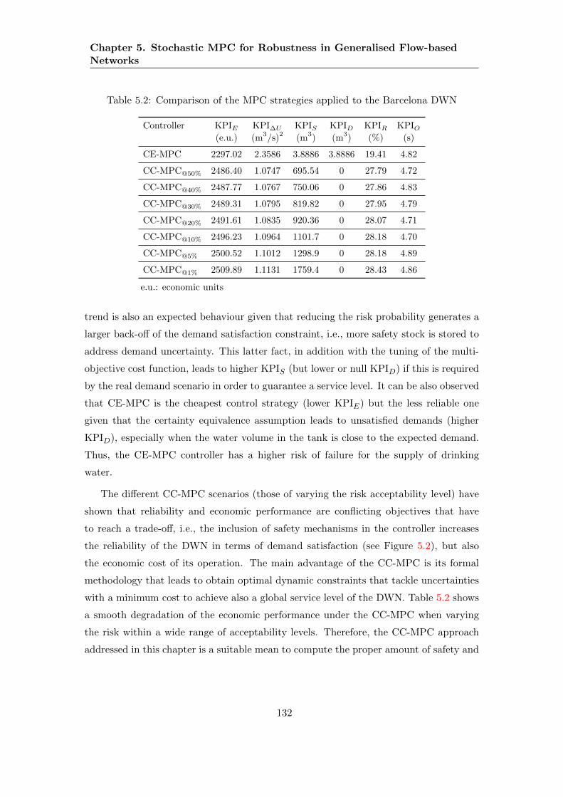
Chapter 5. Stochastic MPC for Robustness in Generalised Flow-basedNetworks
Table 5.2: Comparison of the MPC strategies applied to the Barcelona DWN
Controller KPIE KPI∆U KPIS KPID KPIR KPIO(e.u.) (m3/s)2 (m3) (m3) (%) (s)
CE-MPC 2297.02 2.3586 3.8886 3.8886 19.41 4.82
CC-MPC@50% 2486.40 1.0747 695.54 0 27.79 4.72
CC-MPC@40% 2487.77 1.0767 750.06 0 27.86 4.83
CC-MPC@30% 2489.31 1.0795 819.82 0 27.95 4.79
CC-MPC@20% 2491.61 1.0835 920.36 0 28.07 4.71
CC-MPC@10% 2496.23 1.0964 1101.7 0 28.18 4.70
CC-MPC@5% 2500.52 1.1012 1298.9 0 28.18 4.89
CC-MPC@1% 2509.89 1.1131 1759.4 0 28.43 4.86
e.u.: economic units
trend is also an expected behaviour given that reducing the risk probability generates a
larger back-off of the demand satisfaction constraint, i.e., more safety stock is stored to
address demand uncertainty. This latter fact, in addition with the tuning of the multi-
objective cost function, leads to higher KPIS (but lower or null KPID) if this is required
by the real demand scenario in order to guarantee a service level. It can be also observed
that CE-MPC is the cheapest control strategy (lower KPIE) but the less reliable one
given that the certainty equivalence assumption leads to unsatisfied demands (higher
KPID), especially when the water volume in the tank is close to the expected demand.
Thus, the CE-MPC controller has a higher risk of failure for the supply of drinking
water.
The different CC-MPC scenarios (those of varying the risk acceptability level) have
shown that reliability and economic performance are conflicting objectives that have
to reach a trade-off, i.e., the inclusion of safety mechanisms in the controller increases
the reliability of the DWN in terms of demand satisfaction (see Figure 5.2), but also
the economic cost of its operation. The main advantage of the CC-MPC is its formal
methodology that leads to obtain optimal dynamic constraints that tackle uncertainties
with a minimum cost to achieve also a global service level of the DWN. Table 5.2 shows
a smooth degradation of the economic performance under the CC-MPC when varying
the risk within a wide range of acceptability levels. Therefore, the CC-MPC approach
addressed in this chapter is a suitable mean to compute the proper amount of safety and
132

Chapter 5. Stochastic MPC for Robustness in Generalised Flow-basedNetworks
0 5 10 15 20 250
0.5
1
1.5
2
2.5
3x 10
4
Time [h]
Vo
lum
e [
m3]
Tank #55
Figure 5.2: Comparison of the robustness in the management of water storage in a sampleof tanks of the Barcelona DWN: (blue circle) CC-MPC1%, (black diamond) CC-MPC20%,(red square) CC-MPC50%, (solid green) CE-MPC, (dashed red) Net demand.
the proper control actions to assure a desired service level. Notice that the computational
burden (KPIO) of the CC-MPC is similar to the CE-MPC given that the complexity
of the optimisation problem is not altered, i.e., the number of constraints and decision
variables remain the same. The only extra load that might be added is the computation
of the variance of the disturbances propagated in the prediction horizon. Consequently,
the CC-MPC approach is suitable for RTC of the Barcelona DWN.
Table 5.3 discloses details of the average production and operational costs related
to each strategy. Comparing the CE-MPC controller with the CC-MPC@5% controller
(requiring a reliability of 95%), it can be noticed that the dynamic safety stocks result-
ing within the stochastic approach might lead to an increase of the operational cost,
especially in the electric cost, mainly due to the extra amount of water that is needed
to be moved through the network and allocated in tanks to guarantee that the water
supply will be feasible with a certain probability for future disturbance realisations.
133

Chapter 5. Stochastic MPC for Robustness in Generalised Flow-basedNetworks
Table 5.3: Comparison of daily average economic costs of MPC strategies
Controller Water Cost Electric Cost Daily Average Cost(e.u./day) (e.u./day) (e.u./day)
CE-MPC 23015.42 27195.31 50210.73
CC-MPC@5% 22980.34 28514.71 51495.05
e.u.: economic units
In the sequel the CC-MPC approach is further simulated for a different initial condi-
tion and compared under two different settings to assess the effect of actuators health.
The MPC settings are:
• CC-MPC(1): It is based in the optimisation problem (5.25), i.e., it considers only
the uncertainty related to exogenous water demands.
• CC-MPC(2): It incorporates additionally the actuator health management policy
described in § 4.3, i.e., it considers both the uncertainty of forecast demands and
the uncertainty of the actuator degradation model. In this setting, the optimisation
problem (5.25) is modified by including constraint (4.10c) and a probabilistic form
of constraint (4.10i) with an associated risk level denoted as δz ∈ (0, 1). This
latter chance constraint is approximated following § 5.3, what gives a deterministic
equivalent constraint z(r),k+N |k ≤ zmax(r),k −Φ−1(
1− δzmN
)‖Σ1/2
η I>(r)‖2 for all r ∈Z[1,m], where η ∈ Rnu is a random vector of noise incorporated in the actuator
health degradation process defined in § 4.3, whose components lie in a normal
distribution N(0,Ση). Recall that the actuator degradation management policy
also adapts on-line the weight W∆u in the cost function according to the reliability
of the actuators.
Table 5.4 summarises the performance of each CC-MPC strategy according to eco-
nomic, safety and smoothness indicators (see § 2.4.4). As expected, the CC-MPC(2) has
a higher KPIE than the CC-MPC(1). The reason of this result is the same as in the RB-
MPC(2), i.e., the inclusion of actuators degradation constraints leads to control actions
that sacrifice (if necessary) economic performance in order to guarantee the availability
of actuators for a given maintenance horizon. The rationing of actuators degradation
also leads to increase the smoothness (KPI∆U ), especially due to the operation of pumps
134

Chapter 5. Stochastic MPC for Robustness in Generalised Flow-basedNetworks
Table 5.4: Key performance indicators for CC-MPC
Controller KPIE KPIS KPI∆U
(e.u.) (m3) (m3/s)2
CC-MPC(1) 2390.57 9421.46 1.0223CC-MPC(2) 2761.48 3364.82 2.8664
e.u.: economic units
associated with Tank 55 to Tank 63 in the bottom-right part of the DWN diagram (see
Figure 2.3). With the CC-MPC(1) the volume of water in the aforementioned tanks are
managed near the safety constraints without complete replenishments, while with the
CC-MPC(2) the excursion of water is cyclic within the full range of operation. The ac-
tuators health management policy forces to cycle the operation of several pumps instead
of keeping some of them always active, and therefore require to exploit the full capacity
of the related tanks. The safety performance indicator (KPIS) is drastically higher in
the CC-MPC(1); the reason is that the volume in tanks tends to remain more time in the
limit of constraints, what leads to increase the frequency of violation of safety thresh-
olds. Figure 5.3 illustrates the mentioned behaviour of the system. In general, chance
constraints cause an optimal back-off from real constraints as a risk averse mechanism
to face the non-stationary uncertainty involved in the prediction of states.
Figure 5.4 shows the accumulated degradation of a set of redundant actuators. No-
tice how the CC-MPC(2) smartly decides to decrease the rate of degradation of Actuator
87 (a pump) by distributing the control effort between the other three plotted actu-
ators (which are valves that have lower coefficients of degradation) according to their
flow capacity. This behaviour is equivalent to the one obtained with the RB-MPC(2) in
Chapter 4, the difference is that the chance constrained approach narrows the maximum
level of degradation allowed at each time step according to the uncertainty in the health
prediction model of actuators. The wear process with the CC-MPC(1) is neglected, com-
promising the reliability of the supply infrastructure even if safety stocks are optimally
computed for a reliable service. This latter observation also applies for the RB-MPC(1)
and the CE-MPC approaches discussed in previous chapters.
Table 5.5 details the water production and electricity costs of each CC-MPC strategy.
The CC-MPC(1) has very similar costs to those of the baseline CE-MPC, but with the
benefit of a better handling of constraints, automatic computation of safety stocks and
135

Chapter 5. Stochastic MPC for Robustness in Generalised Flow-basedNetworks
0 24 48 72 960
2000
4000
6000
Tank # 31V
olu
me [m
3]
0 24 48 72 960
100
200
300
400
Tank # 36
Volu
me [m
3]
0 24 48 72 960
10
20
30
40
Tank # 49
Volu
me [m
3]
Time [h]
0 24 48 72 960
1000
2000
3000
Tank # 60
Volu
me [m
3]
Time [h]
xCCMPC
1
xCCMPC
2
xCEMPC
xmax
xmin
xs
dnet
(a) Management of water storage with the CC-MPC strategies
0 24 48 72 96
−0.1
0
0.1
0.2
0.3
Flo
w [m
3/h
]
Actuator # 81
0 24 48 72 96−0.05
0
0.05
0 24 48 72 960
2
Flo
w [m
3/h
]
Actuator # 83
0 24 48 72 96−0.05
0
0.05
0 24 48 72 960
0.5
1
1.5
2
Time [h]
Flo
w [m
3/h
]
Actuator # 84
0 24 48 72 96−0.05
0
0.05
0 24 48 72 960
0.1
0.2
0.3
0.4
0.5
Time [h]
Flo
w [m
3/h
]
Actuator # 87
0 24 48 72 96−0.05
0
0.05
uCCMPC
1
uCCMPC
2
uCEMPC
umax
umin Electric tariff pattern
(b) Management of actuators with the CC-MPC strategies
Figure 5.3: Operation of the Barcelona DWN with the CC-MPC strategies
management of risk near to the output bounds. On the other hand, the CC-MPC(2)
achieves a notorious improvement in electric costs but at the expense of increasing stored
volumes of water (no matter the expensive the source could be) and consequently water
136

Chapter 5. Stochastic MPC for Robustness in Generalised Flow-basedNetworks
0 10 20 30 40 50 60 70 80 90 1000
1
2
3
4
5
6
7x 10
−3
Time [h]
Accum
ula
ted H
ealth
Deg
radatio
n (
Z)
ZCCMPC
1
(81)
ZCCMPC
1
(83)
ZCCMPC
1
(84)
ZCCMPC
1
(87)
ZCCMPC
2
(81)
ZCCMPC
2
(83)
ZCCMPC
2
(84)
ZCCMPC
2
(87)
Figure 5.4: Degradation of a set of redundant actuators under the CC-MPC strategies
costs. Nevertheless, the full approach has the capability to manage actuators health,
and of course, such enhancement implies a higher total cost (if based only on water
and electric prices without considering corrective maintenance costs that probably will
appear if the degradation management is not active to guarantee actuator availability).
The conservatism of reformulating the pure stochastic MPC into the tractable deter-
ministic equivalent CC-MPC is shown in Table 5.6 for the respective chance constraints
associated with the state bounds, safety levels and degradation management, with dif-
ferent levels of maximum joint risk. Notice that the conservatism increases when the risk
level increases but remains constant despite the variation of the number of individual
constraints. Hence, the goodness of the approximation using the Boole’s inequality is
not affected; neither by the number of decision variables, nor by the prediction horizon.
An important aspect in any MPC controller is the handling of constraints. In the
Barcelona DWN, manipulated variables can always be kept within bounds by the con-
troller, but output constraints, which are subject to measured and/or unmeasured un-
certainties, must be controlled in advance. Neither the baseline CE-MPC approach
described in Chapter 2 nor the economic MPC approaches in Chapter 3 consider un-
137

Chapter 5. Stochastic MPC for Robustness in Generalised Flow-basedNetworks
Table 5.5: Water and electric cost comparison of CC-MPC strategies
MPC Approach Water Cost Electric Cost Total Cost(e.u.) (e.u.) (e.u.)
Day 1CC-MPC(1) 21937.42 29074.87 51012.30CC-MPC(2) 45248.32 12176.02 57424.34
Day 2CC-MPC(1) 31300.76 29869.56 61170.32CC-MPC(2) 58707.65 13380.02 72087.68
Day 3CC-MPC(1) 28958.00 29783.34 58741.34CC-MPC(2) 55131.50 13227.99 68359.50
Day 4CC-MPC(1) 28630.73 29939.65 58570.38CC-MPC(2) 53629.68 13600.91 67230.60
e.u.: economic units
certainty explicitly in the controller and might require on-line tuning to ensure an ap-
propriate robust performance, as addressed with the learning-based tuning strategy in
Chapter 6. The other MPC strategies developed so far in this thesis, i.e., RB-MPC,
CC-MPC and TB-MPC, focus on robust performance of the DWN, where flow demand
constitutes the main source of uncertainty. Both the RB-MPC and the CC-MPC strate-
gies enhance the robustness of the baseline CE-MPC by performing a dynamic handling
of constraints while keeping tractability of the optimisation problems even for the large-
scale model of the case study. Instead, the TB-MPC introduces robustness by considering
a single optimisation problem with multiple disturbance scenarios, what precludes the
tractability and limits the applicability of the technique to small-scale systems.
Figure 5.5 shows the mechanism that the RB-MPC and the CC-MPC use to guar-
antee a service level in the DWN and to avoid the violation of real output constraints
due to uncertainty. The plot shows the response of both controllers for a forecasted de-
mand with confidence levels of 80% and 95%. Notice that both approaches dynamically
generate a back-off of original constraints. The characteristics of the safety mechanism
observed in each controller are the following:
• RB-MPC: This controller uses the original output bounds, but computes a dy-
namic soft constraint (i.e., the base stock) to guarantee a desired service level. It
can be seen in the evolution of the base stock that the uncertainty is considered
stationary within the MPC algorithm, i.e., the constraint keeps a uniform back-off
138

Chapter 5. Stochastic MPC for Robustness in Generalised Flow-basedNetworks
Table 5.6: Conservatism of the Deterministic Equivalent CC-MPC
Joint Chance Constraint Number of Individual Joint Risk ConservatismConstraints of Approximation
State Hard Bounds
0.001 4.9967× 10⁻⁷
0.01 4.9817× 10⁻⁵
3024 0.03 4.4539× 10⁻⁴
0.05 1.2290× 10⁻³
0.1 4.8359× 10⁻³
Safety Constraint
0.001 4.9950× 10⁻⁷
0.01 4.9801× 10⁻⁵
1512 0.03 4.4524× 10⁻⁴
0.05 1.2286× 10⁻³
0.1 4.8344× 10⁻³
Degradation Constraint
0.001 4.9965× 10⁻⁷
0.01 4.9816× 10⁻⁵
114 0.03 4.4537× 10⁻⁴
0.05 1.2290× 10⁻³
0.1 4.8358× 10⁻³
of demand, whose amount represents the safety stock along the prediction horizon.
The stochastic description of demands, used to define this soft constraint, is com-
puted a posteriori, based on the sample mean and sample deviation (see § 4.2),
before each MPC execution.
• CC-MPC: This controller incorporates robustness by replacing the deterministic
constraints with chance constraints. In this approach, every constraint that in-
volves random variables is adjusted, hence, either the base stock, the hard bounds
of the states and the terminal constraint of actuators degradation are dynamically
managed by the CC-MPC controller. The level of observed back-off is variable
and depends on the volatility of the forecasted demand at each prediction step
(see § 5.3). In this approach, a prediction model of the stochastic properties of
disturbances is used in parallel with the MPC model.
An important observation regarding the handling of constraints by both RB-MPC
and CC-MPC controllers is the inherent relation between the service level in the RB-
MPC and the joint risk level in the CC-MPC. Despite being defined under different
139
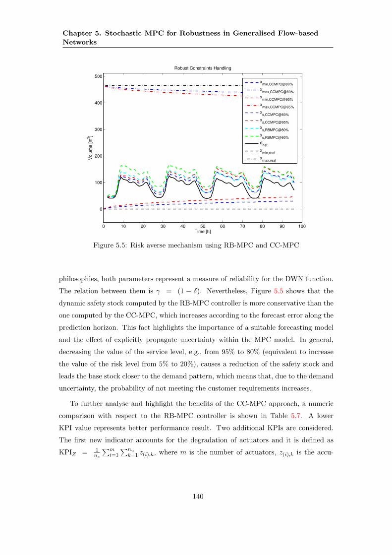
Chapter 5. Stochastic MPC for Robustness in Generalised Flow-basedNetworks
0 10 20 30 40 50 60 70 80 90 100
0
100
200
300
400
500
Robust Constraints Handling
Time [h]
Volu
me [
m3]
xmin,CCMPC@80%
xmax,CCMPC@80%
xmin,CCMPC@95%
xmax,CCMPC@95%
xs,CCMPC@80%
xs,CCMPC@95%
xs,RBMPC@80%
xs,RBMPC@95%
dnet
xmin,real
xmax,real
Figure 5.5: Risk averse mechanism using RB-MPC and CC-MPC
philosophies, both parameters represent a measure of reliability for the DWN function.
The relation between them is γ = (1 − δ). Nevertheless, Figure 5.5 shows that the
dynamic safety stock computed by the RB-MPC controller is more conservative than the
one computed by the CC-MPC, which increases according to the forecast error along the
prediction horizon. This fact highlights the importance of a suitable forecasting model
and the effect of explicitly propagate uncertainty within the MPC model. In general,
decreasing the value of the service level, e.g., from 95% to 80% (equivalent to increase
the value of the risk level from 5% to 20%), causes a reduction of the safety stock and
leads the base stock closer to the demand pattern, which means that, due to the demand
uncertainty, the probability of not meeting the customer requirements increases.
To further analyse and highlight the benefits of the CC-MPC approach, a numeric
comparison with respect to the RB-MPC controller is shown in Table 5.7. A lower
KPI value represents better performance result. Two additional KPIs are considered.
The first new indicator accounts for the degradation of actuators and it is defined as
KPIZ = 1ns
∑mi=1
∑nuk=1 z(i),k, where m is the number of actuators, z(i),k is the accu-
140

Chapter 5. Stochastic MPC for Robustness in Generalised Flow-basedNetworks
Table 5.7: Comparison of controllers performance
Controller KPIE KPIS KPI∆U KPIZ KPIV KPIO CPU Time
(e.u.) (m3) (m3/s)2 (s) (s)
CE-MPC 2442.97 0.18011 0.8419 0.1374 2245 1.83 202.37
RB-MPC(1)@95% 2383.97 1987.75 0.9024 0.1377 1596 10.22 884.10
RB-MPC(2)@95% 2569.59 3029.94 2.1023 0.1098 1699 9.18 892.34
RB-MPC(1)@80% 2373.44 991.68 0.8265 0.1376 1775 9.01 878.19
RB-MPC(2)@80% 2560.72 1625.29 2.0665 0.1187 1761 9.17 891.38
CC-MPC(1)@5% 2390.57 9421.46 1.0223 0.1373 1822 2.65 624.36
CC-MPC(2)@5% 2761.48 3364.82 2.8664 0.1270 1710 2.50 603.91
CC-MPC(1)@20% 2362.64 710.22 1.1556 0.1374 1960 2.41 603.61
CC-MPC(2)@20% 2560.36 4946.13 2.2038 0.1076 1715 2.67 629.35
e.u.: economic units
mulated health degradation of the i-th actuator at time step k, and ns is the simulation
horizon of the assessment. The second new indicator measures the number of safety
constraint violations that have been occurred during the simulation and it is defined as
KPIV =∑ns
k=1 nv,k, where nv,k is the number of tanks that required the use of its safety
stock at time step k. Simulations have been carried out using γ = 80, 95% for the RB-
MPC and δ = 5, 20% for the CC-MPC. In addition, Table 5.8 and Figure 5.6 disclose
details of the production and operational costs related to each strategy, which are the
primary objectives for managers. Furthermore, Table 5.9 summarises the capabilities
handled by each controller. This qualitative information complements the quantitative
evaluation of the strategies in order to highlight the benefits of the MPC designs.
After reviewing the performance indicators and capabilities, it can be reaffirmed that
the robust MPC strategies developed in this thesis outperform the CE-MPC controller,
which may have low values in most of the KPIs but with any guarantee of reliability,
robust or probabilistic feasibility. Despite to have the lowest KPIS , the baseline ap-
proach is the one that presents the highest number of soft constraints violations, what
means that the safety thresholds might be overestimated (as observed in several tanks
in the DWN), causing more oscillations in the excursion of water, or keeping states near
the threshold with easiness to activate the constraints in the controller. Therefore, the
141

Chapter 5. Stochastic MPC for Robustness in Generalised Flow-basedNetworks
Table 5.8: Comparison of daily average costs of MPC strategies
MPC Approach Water Average Cost Electric Average Cost Daily Average Cost(e.u./day) (e.u./day) (e.u./day)
CE-MPC 29037.21 29594.14 58631.35
RB-MPC(1) 27756.93 29580.78 57337.72
RB-MPC(2) 42072.97 19597.27 61670.25
CC-MPC(1) 27706.72 29666.85 57373.58
CC-MPC(2) 53179.29 13096.23 66275.53
e.u.: economic units
0 1 2 3 40
0.5
1
1.5
2
2.5
3x 10
4 Daily Electric Costs
Ele
ctr
ic C
ost
[e.u
.]
Time [day]0 1 2 3 4
0
1
2
3
4
5
6x 10
4 Daily Water Costs
Wa
ter
Co
st
[e.u
.]
Time [day]
CEMPC RBMPC(1)
RBMPC(2)
CCMPC(1)
CCMPC(2)
0 24 48 72 960
0.1
0.2
0.3
0.4
0.5Hourly Electric Costs
Time [h]
Ele
ctr
ic C
ost
[e.u
.]
0 24 48 72 960
0.2
0.4
0.6
0.8Hourly Water Costs
Time [h]
Wa
ter
Co
st
[e.u
.]
Figure 5.6: Comparison of hourly and daily costs
baseline CE-MPC approach, with fixed and empirical safety stocks, limits the economic
optimisation. Instead, the strategies RB-MPC(1) and CC-MPC(1), reached the lowest
KPIE (in both 80% and 95% risk levels) by incorporating robust and optimal safety
142

Chapter 5. Stochastic MPC for Robustness in Generalised Flow-basedNetworks
Table 5.9: Comparison of capabilities handled by each controller
.
Controller Dynamic Dynamic Actuators SmartSafety Stocks Output Bounds PHM Tuning
CE-MPCRB-MPC(1)
√RB-MPC(2)
√ √ √CC-MPC(1)
√ √CC-MPC(2)
√ √ √ √√: handled
stocks to face demand uncertainty with minimum storage of water. These robust ap-
proaches have lower KPIV , i.e., they reduce the number of violations of the base stocks,
but increase the amount of safety stocks used to meet demands (higher KPIS). This is
an expected behaviour due to the policy of minimum storage behind the computation of
the base stocks, which prefers to use the safety stocks instead of keeping more volume
of water than the required. The lower cost of water in the Barcelona DWN (see Fig-
ure 5.6), comparing the CE-MPC with the RB-MPC(1) and CC-MPC(1), reinforces this
observation. The main disadvantage of these cheaper controllers is that control actions
are computed based on economic criteria and accounting for tanks reliability but not for
actuators reliability. This fact leads to higher values of the KPIZ , i.e., the controllers
overexploit those actuators that have lower operational costs, accelerating their wear
and compromising the service reliability.
In order to manage the overall system reliability, the RB-MPC(2) and CC-MPC(2)
controllers incorporate actuators health models and restrict their maximal cumulative
degradation at each time step to ensure their proper functioning until a maintenance
horizon is reached. As seen in Table 5.8, the ability to compute control actions for
an efficient management of actuator reliability implies an important reduction of the
electric costs, but at expense of an increment of the KPIE due to the higher water
cost, of the KPI∆U due to the distribution of control effort that avoids (if possible)
constant control actions that could cause an imbalance degradation of actuators, and
of the KPIS due to the narrowing of constraints. It is important to point out that
the two RB-MPC controllers have greater KPIO than the CC-MPC controllers. The
reason is that the former ones have to solve a bi-level optimisation problem on-line,
compared with the CC-MPC controllers that just require to solve a single optimisation
143

Chapter 5. Stochastic MPC for Robustness in Generalised Flow-basedNetworks
problem. Nonetheless, all the compared controllers are suitable for RTC considering the
sampling time in the DWN is one hour. Looking at the results discussed before, the
CC-MPC strategy should be preferred given their tractability for large-scale systems (as
shown with the Barcelona DWN case study) and its ability to handle probabilistic and
deterministic constraints.
5.6 Summary
In this chapter, two stochastic control approaches have been assessed to deal with the
management of generalised flow-based networks. Both the CC-MPC and the TB-MPC
approaches focused on robust economic performance under additive disturbances (un-
bounded and stationary or non-stationary) and avoid relying on heuristic fixed safety
volumes such as those used in the CE-MPC or the RB-MPC schemes proposed in the
previous chapters, which results in better economic performance. According to the re-
sults obtained for the considered case study, both techniques showed a relatively similar
performance. However, it seems clear that CC-MPC is more appropriate when requiring
a low probability of constraint violation, since the use of TB-MPC demands the inclusion
of a higher number of scenarios, which may be an issue for the application of the latter to
large-scale networks. The analytical approximation of joint chance constraints based on
their decomposition into individual chance constraints, these latter bounded by means
of Boole’s inequality, has shown to be suitable for large networks regarding that the
conservatism involved is not affected neither by the number of the inequalities nor the
prediction horizon of the MPC. The level of resultant back-off is variable and depends on
the volatility of the forecasted demand at each prediction step and the suitability of the
probabilistic distribution used to model uncertainty. The presence of unbounded distur-
bances in the system precludes the guarantee of robust feasibility with these schemes.
Hence, the approaches proposed in this chapter are based on a service-level guarantee
and a probabilistic feasibility. The case study shows that the CC-MPC is suitable for
the operational guidance of large-scale networks due to its robustness, flexibility, modest
computational requirements, and ability to include risk considerations directly in the
decision-making process. Even when the CC-MPC increased the operational costs by
around 2.5%, it allowed to improve service reliability by more than 90% when comparing
with a CE-MPC setting.
144

Chapter 5. Stochastic MPC for Robustness in Generalised Flow-basedNetworks
Future research will be directed to incorporate parametric uncertainty and unmea-
sured disturbances in the model. In addition, future work should include a more detailed
study regarding the number of scenarios contained in the tree. Likewise, distributed com-
putation could be used in order to relieve the scaling problems of TB-MPC when the
number of scenarios is too high. Moreover, it is of interest to extend the results and de-
velop decentralised/distributed stochastic MPC controllers for large-scale complex flow
networks.
145


Chapter 6
Learning-based Tuning ofSupervisory MPC for GeneralisedFlow-based Networks
This chapter proposes a synergy of artificial intelligence, supply chain theory and auto-
matic control to devise an adaptive and robust MPC controller for the management of
generalised flow-based networks. Here, a Learning-based Supervisory MPC (LB-MPC)
strategy with a hierarchical multilayer structure is developed, where soft-computing
techniques (i.e., neural networks and fuzzy logic) are used not to approximate an MPC
controller but to tune its design parameters on-line by learning the expectation of the
performance. In contrast to general tuning approaches, the LB-MPC method presented
in this chapter not only adapts the weights of the multi-objective optimisation problem
that takes place within the MPC controller but also the prediction horizon according
to the current situation of the plant. Furthermore, operational output constraints are
dynamic and governed according to the non-stationary uncertainty of the system distur-
bances to assure service reliability while optimising economic resources. The proposed
control scheme is a quasi-explicit MPC approach with low on-line computational burden,
because most of the heavy computations are converted into non-linear explicit modules
using neural networks. The benefits, i.e., flexibility and reliability of this LB-MPC con-
troller as a decision-support tool are shown in this chapter through the real case study
of § 2.4.
147

Chapter 6. Learning-based Tuning of Supervisory MPC for GeneralisedFlow-based Networks
6.1 Control System Structure
The control strategy addressed in this chapter is based on a multilayer (hierarchical)
control system structure. The hierarchical architecture has been frequently used in pro-
cess control with satisfactory results optimising economic profits when disturbances are
slowly varying [174]. In several generalised flow-based network applications and partic-
ularly in the case study addressed in this thesis, disturbances often follow a pattern in
a daily basis and can be well predicted for an hourly sampling time, which makes the
hierarchical structure suitable to optimise targets for the policies of the direct control
level. Therefore, the controller proposed in this chapter is based on a three-layer struc-
ture (see Figure 6.1). First, a Learning and Planning layer (LPL) determines on-line
strategic dynamic safety constraints, economically optimal state references and demand
forecasts, all of them by means of artificial neural networks (ANNs). Secondly, a Su-
pervision and Adaptation layer (SAL) implements a fuzzy rule-based inference system
(FIS) to continually adjust the parameters of an MPC controller, which computes, along
the receding horizon approach, the optimal controlled flows according to the current
status of the plant. Finally, a Basic Feedback Control layer (BFCL), commonly based
on PID controllers or any other tracking-oriented controller, is responsible for real-time
operation of the system and has direct access to the manipulated variables. The BFCL
is not addressed in this chapter because it is assumed that the design problem of each
local regulatory controller is already solved by the operators of the system. Hence, as a
common practice in the design of hierarchical controllers, perfect reference tracking of
the control loops at the lower layer is assumed in this chapter.
6.2 Learning and Planning Layer
Classical hierarchical MPC structures exhibit a high computational burden when set-
point optimisation, governing of constraints and forecasting of disturbances, are required
to be executed at the same frequency that the control problem is solved. Sequential opti-
misations are often required for the planning of actions in top layers but many parameters
and non-linear functions cause these tasks to be intractable for on-line tuning of con-
trollers, especially in large-scale systems as generalised flow-based networks. Therefore,
148

Chapter 6. Learning-based Tuning of Supervisory MPC for GeneralisedFlow-based Networks
General Management Policies
Learning and Planning
Supervision and Adaptation
Basic Feedback Control
Plant
(Neural-Networks based)
(Fuzzy-tuned MPC)
dDisturbance(Real demand)
u y
xu⋆
d, xe, s x, V 0
N(k, x)
V 0
N(k, x)Service Level
Prices
Constraints
Priorities
Weather conditions(Temperature, humidity)
Knowledge base(rules, fuzzy-sets)
Figure 6.1: Multilayer hierarchical intelligent control architecture
this chapter proposes a planning layer that uses ANNs in order to reduce the computa-
tional burden of optimisation-based approaches.
ANNs have a remarkable ability to derive meaning from complicated or imprecise
data and can be employed to extract patterns and detect trends that are too complex to
be noticed by other computational techniques. Specifically, this chapter uses multi-layer
perceptron (MLP) neural models, which as proved in [44, 61] can represent continuous
functions to any degree of accuracy, with at least one hidden layer, provided that the
number of neural units is sufficiently large. MLP is considered a universal approximator
and has been efficiently used for on-line predictive control due to its natural capability for
storing and generalising experience-based knowledge, see e.g., [60, 98, 141]. As illustrated
in Figure 6.2, a basic MLP consists of one input layer containing a vector of N ∈ Z≥1
predictor variable values (z1, . . . , zN )>, one or more hidden layers with S ∈ Z≥1 active
neurons, and one output layer with L ∈ Z≥1 neurons. Learning is a process through
which free parameters (i.e., synaptic weights whji and wokj , and bias levels bhj and bok,
with i ∈ Z[1,N ], j ∈ Z[1,S], k ∈ Z[1,L]) of an ANN are adapted through a continuous
process of stimulation by the environment in which the network is embedded. In this
chapter, three MLP supervised training structures (see Figure 6.3) with one hidden
layer are devised in order to forecast flow demands and to plan future base-stocks and
economically optimal references. Tan-sigmoid and linear activation functions are used
for the hidden and the output layers, respectively, following the results presented in
149

Chapter 6. Learning-based Tuning of Supervisory MPC for GeneralisedFlow-based Networks
b
b
b
b
b
b
b
b
b
b
b
b
b
Input Hidden Output
Σ
Σ
Σ
Σ
Σ
Σ
f h
f h
f h
f o
f o
f o
yo1
yok
yoL
no1
nok
noL
yh1
yhj
yhS
nh1
nhj
nhS
woLS
bhS
bhj
bh1
1
1
1
1
1
1
wh11
whS N
z1
z2
zi
zN
yh= f h(Whz + bh) yo
= f o(Woyh+ bo)
wo11
bo1
bok
boL
Figure 6.2: Feed-forward Neural Network diagram
[192]. The training patterns (i.e., 8640) used in each ANN are divided randomly with a
ratio of 60%, 20% and 20%, to form training, validation and testing sets, respectively.
Networks with different numbers of active neurons have been trained off-line in order
to find the one with the smallest test data cost. The training of the ANNs is done
with the Gauss-Newton approximation to Bayesian regularisation (GNBR) algorithm
developed in [46], which avoids over-fitting and improves the generalisation ability of
the neural models. This training method performs Bayesian regularisation employing
the Levenberg-Marquardt back-propagation algorithm, which ensures that the ANNs
provide accurate output values for inputs not represented in the calibration set of the
neural network and imposes constraints to get smaller weights and a smoother ANN
behaviour.
6.2.1 ANN for Demand Forecasting
This module focuses on the problem of flow demand forecasting for real-time operation of
a given generalised flow-based network. An hourly consumption data analysis is proposed
here for training an MLP (see Figure 6.3 top) with 100 neurons in the hidden layer. For
the particular DWN case study (see § 2.4), the inputs to the neural model are chosen
based on the suggestions in [11] and correlation analysis, i.e., considering consumption
data and meteorological variables such as temperature T and air relative humidity H.
Principal component analysis (PCA) preprocessing is applied to the training patterns
150

Chapter 6. Learning-based Tuning of Supervisory MPC for GeneralisedFlow-based Networks
+−
BP
dkANND
Tk
Hk
ed,k
dk
+−
b
b
ANNE
BP
tk
dk
ee,k
xe,k xk uk
ℓE
SystemEconomic
MPC
pk X,U
dk
+−ANNS
BP
dk
es,k
sk sk uk
ℓE
Base Economic
MPC
pk X,U
dk
Stocks
+
−
bdk
ed,k
γ τ D
DB ed,k
Figure 6.3: ANNs training diagrams for Demand Forecasting (top), Economic trajectory(middle) and Base-stocks setting (bottom)
in order to reduce the dimension of the input vectors and to obtain uncorrelated values
that facilitate the learning process.
6.2.2 ANN for Optimal Economic Trajectory
The economically optimal state trajectory for each flow storage unit is the one obtained
considering only the economic stage cost term `E : Z+×X×U→ R+ of a possibly multi-
objective cost function related to the operation of the network flows, solving often a
linear programming constrained optimisation problem on-line. Again, for the particular
case study in § 2.4, and with the intention to reduce computational effort, an MLP
with 50 neurons in the hidden layer is trained off-line to emulate the economic MPC
controller. A non-linear explicit approximated model of the optimal operation of the
system is obtained, which is later used to compute at each time step k ∈ Z+ the economic
trajectory xe,k = xe,k+ii∈Z[0,N ]for a given prediction horizon N ∈ Z≥1, taking into
account the known economic parameter pk involved in the stage cost `E , the constraint
sets and the predicted demand sequence dk as inputs (see Fig. 6.3 middle).
151

Chapter 6. Learning-based Tuning of Supervisory MPC for GeneralisedFlow-based Networks
6.2.3 ANN for Dynamical Safety Volumes
In order to include the safety stock management policy proposed in § 4.2, this chapter
uses an ANN to avoid the on-line optimisations that are required to virtually decouple
the dynamic states of a generalised flow-based network for the calculation of the base-
stock vector in (4.4). Here, the non-linear explicit approximated model of a trained MLP
dynamically computes the safe base-stock vector sk ∈ Rn for each k ∈ Z+ (see Figure 6.3
bottom). For the particular case study in § 2.4, an MLP with 50 neurons in the hidden
layer is trained with input-output patterns that are generated using historical records of
demand forecasting errors ed,k ∈ Rp as inputs, while using safety inventories in sk ∈ Rn
as outputs. The target sk of this ANN has been calculated following § 4.2 with a service
level γ = 95% and a lead time τ = 4 hours.
Remark 6.1. The number of hidden layers and neuron units depend upon the complexityof the problem and the available computational resources, i.e., both are design parameters.
♦
Remark 6.2. Neural models may not adapt to all characteristics of the environment,especially when there are uncertainties and no feedback correction mechanisms. Theperformance of ANNs in any application will be as adequate as the scenarios and thequality of the training data set are. This lack of guarantees is the reason why this chapterenhances a constrained MPC controller with neuro-learning for tuning purposes insteadof implementing a pure neuro-control approach. ♦
6.3 Supervision and Adaptation Layer
Self-tuning on-line algorithms for MPC of large-scale flow networks is not a widely re-
ported topic in literature. Most of the tuning strategies for the inherent multi-objective
optimisation problems take into account the exploration of the complete Pareto frontier
to choose a non-dominated solution in line with the management objectives. As shown
in [178] for a water network application, one of the goals behind the Pareto frontier
applied to the predictive control of a generalised flow-based network should be to find a
direct relation between the weights of the solution points and the flow demands, which
often are assumed periodic as discussed in Chapter 3. Nevertheless, the computation of
the Pareto frontier for a given system and cost function could be cumbersome. There-
fore, to reduce computational complexity, this chapter presents an adaptation scheme,
similar to the one in [4]. Here, a fuzzy logic module interacts with an MPC controller by
152

Chapter 6. Learning-based Tuning of Supervisory MPC for GeneralisedFlow-based Networks
Fuzzification Defuzzification
R1(eE , eS )
R2(eE , eS )
Rr(eE , eS )
Knowledge Base
Rules-based Inference
eE , eS N,We,Ws,W∆u
LinkingHeuristic
Figure 6.4: Fuzzy rules-based MPC tuner diagram
automatically adjusting the tuning parameters of the controller based on the supervision
of output feedback and measured disturbances.
6.3.1 Reasoning Mechanism
A knowledge-based tuner for the MPC controller is proposed in the sequel. The tuning
mechanism consists in a fuzzy inference system (FIS) that involves: (i) a fuzzyfication
interface, (ii) an a priori rule base, (iii) a defuzzyfication interface, and (iv) a linking
heuristic (see Figure 6.4). The design of each of these elements is application-dependent
and should be set up after a phase of experimentation and understanding of the effect
that the selected tuning parameters have on the given generalised flow-based network.
Hence, the methodology is next explained for the case study of § 2.4.
First, a fuzzyfication phase converts the crisp values of both the normalised economic
state error defined as eE,k := |xk − xe,k|/xe,k ∈ Rn and the normalised safety volume
state error defined as eS,k := (xk − sk)/sk ∈ Rn, into fuzzy values. Indeed, to each input
of the supervisor nifs input fuzzy sets are associated and labelled with nifs linguistic
input variables and described by specific Gaussian membership functions with values in
the interval [0, 1]. The universe of discourse for the input eE is: small (S), medium (M),
large (L); and for the input eS it is: large-negative (LN), medium-negative (MN), small-
negative (SM), very-small-negative (V SN), very-small-positive (V SP ), small-positive
(SP ), medium-positive (MP ), large-positive (LP ).
153

Chapter 6. Learning-based Tuning of Supervisory MPC for GeneralisedFlow-based Networks
Table 6.1: Fuzzy-logic rules for LB-MPC.
Rule Inputs Outputs
eE,k eS,k Nk We,k Ws,k W∆u,k
1 L LP L L VS VS2 L MP L L VS S3 L SP L M VS M4 L VSP L S S L5 M LP M L VS VS6 M MP M L VS S7 M SP M M VS M8 M VSP M S S L9 S LP S L VS VS10 S MP S M VS S11 S SP S M VS M12 S VSP S S S L13 any LN L VS L VS14 any MN L VS L VS15 any SN L VS L VS16 any VSN L VS L VS
The fuzzy-logic supervisor involves expert knowledge using the Mamdani’s fuzzy
inference system, which applies the set of linguistic rules presented in Table 6.1 to
the fuzzy inputs in order to evaluate the supervisor fuzzy outputs. The inference ta-
ble associates nofs output fuzzy sets (nofs linguistic output variables), described by
specific trapezoidal membership functions, to the supervisor’s crisp output variables
Nk, We,k, Ws,k, W∆u,k ∈ Rn, k ∈ Z+. The universe of discourse for output Nk is: small
(S), medium (M), large (L); and for the outputs We,k, Ws,k, W∆u,k is: very small
(V S), small (S), medium (M), large (L). The min-max inference method is used for
the evaluation of the fuzzy rules contribution, and the gravity center method is used in
the defuzzyfication phase. For a detailed explanation on fuzzy inference reasoning, the
reader could refer to [185]. Note that the outputs of the FIS are in Rn because they are
computed for every state in the network. Therefore, it is further required to transform
the resulting weights We,k and W∆u,k into an actuator base in Rm×m and the results for
Nk into an integer value N ∈ Z≥1. The weight Ws,k is already related to states but it
has to be transformed into a diagonal matrix in Rn×n.
154

Chapter 6. Learning-based Tuning of Supervisory MPC for GeneralisedFlow-based Networks
6.3.2 Linking Heuristic
To obtain the quantitative value of the tuned parameters in the corresponding domain for
the MPC problem stated in § 2.4.3, an associative heuristic is proposed in Algorithm 2,
where the argument of sub-index (·) represents a specific row of the associated variable.
This heuristic is based on the topology of the generalised flow-based network.
Algorithm 2 Linking Heuristic
1: procedure LinkingHeuristic(We,k, Ws,k, W∆u,k, Nk)2: m := number of actuators3: n := number of tanks4: we ← 0m×1
5: w∆u ← 0m×1
6: for i = 1→ m do7: if u(i) connects junction–junction or storage–demand then8: we(i) ← 09: w∆u(i) ← 0
10: else11: if u(i) connects storage(a)–storage(b) , with a, b ∈ Rn then
12: we(i) ← maxWe(a),k, We(b),k13: w∆u(i) ← maxW∆u(a),k, W∆(b),k14: else15: if u(i) connects storage(a)–junction , with a ∈ Rn then
16: we(i) ← We(a),k
17: w∆u(i) ← W∆u(a),k
18: end if19: end if20: end if21: end for22: We ← Rm×m (diagonal matrix whose diagonal is the vector we)23: W∆u ← Rm×m (diagonal matrix whose diagonal is the vector wu)24: Ws ← Rn×n (diagonal matrix whose diagonal is the vector Ws,k)
25: N ← maxNk26: return N,We,Ws,W∆u
27: end procedure
Remark 6.3. Most of the tuning guidelines reported in literature assume weighting ma-trices with equal elements in the diagonal. The learning-based tuning approach presentedin this thesis allows to adapt on-line individual elements of the cost function weightingmatrices giving more degrees of freedom to the managers of the network. ♦
155

Chapter 6. Learning-based Tuning of Supervisory MPC for GeneralisedFlow-based Networks
Table 6.2: Performance of the ANNs (MAE%)
Neurons ANNd ANNe ANNs
10 8.8299 629.4652 3.5512
20 7.1257 87.2827 2.0423
30 10.9843 89.3765 1.5513
40 7.8918 1.4455 1.4124
50 8.6294 1.4098 1.0376
60 11.2109 1.4263 1.0323
70 11.3223 1.4788 1.0206
80 7.4649 − −90 14.0614 − −100 6.6945 − −110 14.8369 − −
6.4 Numerical Results
In this section, simulation results of the LB-MPC approach applied to the aggregate
model (see Figure 2.4) of the DWN case study described in § 2.4 are presented. All
the simulations have considered a time period of four days (96 hours). The selected
sampling time is one hour. Simulations have been carried out using the CPLEX solver
of the TOMLAB 7.6 optimisation package, together with the Fuzzy Logic Toolbox and
the Neural Network Toolbox of Matlab R2010b (64 bits). The computer used to run the
simulations is a PC Intel Core E8600 running both cores at 3.33GHz with 8GB of RAM.
6.4.1 Demand Forecasting and States Planning with ANNs
Table 6.2 shows the mean absolute percentage error (MAE%) of the ANNs described
in § 6.2, that were trained using the function trainrb included in the Neural Network
Toolbox of Matlab. The final architecture of each ANN was selected by comparing the
performance of experiments varying the number of neurons in the hidden layer. The
selected number of neurons were 100, 50 and 50 for the ANNd, ANNe, and ANNs,
respectively. Forecasting of demand with the ANNd is based on water consumption and
meteorological (temperature and air relative humidity) records available from AGBAR
Company and from the Servei de Meteorologia de Catalunya1, respectively. The results
1http://www.meteo.cat
156

Chapter 6. Learning-based Tuning of Supervisory MPC for GeneralisedFlow-based Networks
show the prediction of water demand is reliable and the magnitude of the forecasting
error is not a reason to reject the obtained model. In fact, these minimal discrepancies
are reflected in an increase of the safety volume. In contrast to ANNd, the ANNe for
the economic optimal trajectory and the ANNs for the safety volume trajectory perform
with higher accuracy as it could be expected, because both MLPs are trained with
the solution of QP problems instead of experimental driven data as in the forecasting
demand case. The advantage of all of the neural models used in this chapter is that the
time invested in processing data and training the ANNs will be gained in the on-line
solving process once they are accurately validated and tested.
6.4.2 Fuzzy Tuning of MPC Parameters
In most of the results presented in literature for control of DWNs, tuning is focused
on the weighting matrices with no adaptation schemes. Nevertheless, for large-scale
systems, an efficient selection of the prediction horizon is demanded since the size and
complexity of the optimisation problem is based mainly on this parameter. Thus, the
methodology proposed in this chapter adapts the prediction horizon according to a trade-
off between risk and economic cost. The selected tuning parameters for problem (2.23)
are the prediction horizon N and the weights We, Ws, W∆u. These parameters were
computed and adapted by the FIS described in § 6.3 using the Fuzzy Logic Toolbox of
Matlab. The evolution of such parameters is shown in Figure 6.5, while the histograms
of their values are shown in Figure 6.6. These results were obtained for an unmeasured
random disturbance of at most 20% of the nominal demand pattern.
6.4.3 LB-MPC Controller for DWN
The proposed learning-based approach has been implemented for the tuning of the con-
strained MPC described in § 2.4.3 to operate the Barcelona DWN. Results have been
compared with two other strategies. The controllers are the following ones:
• MPCo: the baseline MPC approach introduced in § 2.4.3, which uses a fixed
prediction horizon (N = 24 hours), constant water base-stocks and constant tuning
weights for the prioritisation of management objectives.
157

Chapter 6. Learning-based Tuning of Supervisory MPC for GeneralisedFlow-based Networks
0 20 40 60 80 1000
5
10
15
20
T ime [hours]
N:Pre
dictionhorizon
[hours]
0 20 40 60 80 10050
60
70
80
90
T ime [hours]
We:Economic
weight
0 20 40 60 80 1004
6
8
10
12
14
16
T ime [hours]
Ws:Safe
tyweight
0 20 40 60 80 1000
10
20
30
40
T ime [hours]
W∆u:Smooth
ness
weight
Figure 6.5: Evolution of tuning parameters for the LB-MPC strategy
• MPCss: the bi-level RB-MPC approach described in Chapter 4, but implementing
only the dynamic optimisation of safety stocks following Section 4.2. It considers
fixed prediction horizon and fixed weights as well.
• LB-MPC: the learning-based MPC approach addressed in this chapter, consisting
in the same problem (2.23) but with adaptive prediction horizon, tuning weights
and safety stocks.
Table 6.3 shows the specific performance indicators (as defined in § 2.4.4) that were
used to assess the aforementioned controllers over the simulation period (Ns = 96 hours).
Recall that KPIE is the total economic cost of the DWN operation, KPIS is the accu-
mulation of all safety level violations and KPI∆U is the accumulated RMS of control
variations. Simulations show that static MPC design parameters (safety stocks, tuning
weights and prediction horizon) are a drawback for the management of network flows,
158

Chapter 6. Learning-based Tuning of Supervisory MPC for GeneralisedFlow-based Networks
0 5 10 15 200
20
40
60
80
100
N Histogram
N : P redi c t i on Hori zon
Frequency
50 60 70 80 900
5
10
15
20
25
W e Histogram
W e: E conomic We ight
Frequency
5 10 15 200
5
10
15
20
25
30
W s Histogram
W s: Safe ty We ight
Frequency
0 10 20 30 400
5
10
15
20
25
W∆u Histogram
W∆u: Smoothne ss We ight
Frequency
Figure 6.6: Histograms of tuning parameters for the LB-MPC strategy
because under uncertain disturbances, the fixed value of these parameters might cause
an undesired restriction of the solution space that degrades the economic performance,
and/or increment the risk of constraint violation. Figure 6.7 shows the excursion of
water in a tank of a representative part of the Barcelona DWN, whose behaviour is rep-
resentative of most storages in the DWN. It can be seen that all of the compared MPC
controllers keep the volume in tank within the hard and soft constraints satisfying also
the net demand along the simulation horizon but with differences in the computational
time (see Table 6.3) and the management of safety stocks that impacts the aforemen-
tioned KPIs. As expected, the safety stocks of the LB-MPC controller tend to reproduce
the ones computed with the MPCss controller because this latter was used to train the
ANN that predicts the safety level in the LB-MPC.
159

Chapter 6. Learning-based Tuning of Supervisory MPC for GeneralisedFlow-based Networks
Table 6.3: Key performance indicators for the different approaches
Controller KPIE (103) KPIS KPI∆U CPU time
(e.u.) (m3) (m3/s)2 (s)MPCo 183.74 28.8022 0.1318 142.01MPCss 176.77 5.0295 0.1340 286.17
LB-MPC 178.99 5.2138 0.1172 132.91
e.u.: economic units
0 24 48 72 96
0
1
2
3
4
5
6
7
8
9
10
x 104 Tank # 12
Vo
lum
e [
m3]
Time [h]
x
MPCo
xMPCss
xLB−MPC
xs,MPCo
xs,MPCss
xs,LB−MPC
dnet
xmax
xmin
Figure 6.7: Dynamic variation of tanks volumes for the different approaches
The MPCo controller presents the highest economic cost due to the conservative and
static safety volumes that limits the economic optimisation. In general, this approach
does not guarantee optimal results for any condition because the safety is fixed heuris-
tically without taking into account demand variations. Instead, the MPCss controller
has a certain robustness to disturbances by optimising the dynamic safety stocks (see
Figure 6.7) in accordance to the deviation of the forecasting error. The MPCss presents
the best economic performance but the highest computational effort (see Table 6.3) since
it involves more on-line optimisation problems to set those safety stocks.
Results show that the LB-MPC controller outperforms the previous strategies. It
presents similar results to the MPCss controller for the economic, safety and smoothness
indicators but reduces the computational burden (see Table 6.3). In addition, Figure 6.7
and Figure 6.8 show that, despite the similar safety stocks of the MPCss controller and
160

Chapter 6. Learning-based Tuning of Supervisory MPC for GeneralisedFlow-based Networks
1 2 3 42.05
2.1
2.15
2.2x 10
4
Time [days]
Eco
no
mic
un
its [
e.u
.]
Daily Electric Costs
MPCo
MPCss
LB−MPC
1 2 3 41
1.5
2
2.5
3x 10
4 Daily Water Costs
Time [days]
Eco
no
mic
un
its [
e.u
.]
MPCo
MPCss
LB−MPC
Figure 6.8: Comparison of the daily electric and water costs for the different approaches
the LB-MPC controller, this latter makes better use of hydraulic and economic resources
due to its flexibility to self-adapt the parameters of the controller if the operational
conditions change (see Figure 6.6). This capability helps managers to deal with demand
uncertainty and prediction errors in an optimal and economic way, guaranteeing the
desired safety and service level with less volume of water and less electric energy.
Furthermore, Figure 6.8 details that even when the MPCss approach has a lower value
than the LB-MPC approach for the economic performance indicator (see Table 6.3),
which integrates water costs and electric costs, the LB-MPC presents a lower cost in
the electric component due to the adaptation of weights by means of the AI techniques
used in this application. From an operational point of view, this difference in costs
implies that the LB-MPC controller decides to take water from more expensive sources
in order to further reduce the electrical costs by pumping more, with respect to the other
approaches, when the electric tariff is cheaper.
161

Chapter 6. Learning-based Tuning of Supervisory MPC for GeneralisedFlow-based Networks
6.5 Summary
This chapter has presented a multilayer MPC approach with self-tuning capabilities for
the efficient management of network flows based on soft-computing techniques. The
approach has been applied to the aggregate model of the Barcelona DWN obtaining
important improvements in the computation time towards on-line implementation for
large-scale systems. The selected tuning parameters of the MPC problem were the pre-
diction horizon and the weighting matrices of the multi-objective cost function. The
main advantage of the fuzzy tuner is its ability to adapt every element independently,
which is a difficult task in analytical approaches due their lack of intuitiveness for multi-
variable large-scale systems. The controller also tunes the set-points based on inventory
management theory, enriching the controller design with reliability aspects to assure
a customer service level under disturbances uncertainty. Further research will be con-
ducted in using other ANNs structures and in reinforcement learning algorithms with
two main directions: (i) to implement intelligent distributed MPC of generalised-flow
based networks where shared variables are negotiated using learning techniques, and (ii)
to adapt and improve the presented fuzzy inference system.
162

Part III
Distributed Economic MPCSchemes for Network
Management
163


Chapter 7
Multi-Layer Non-IterativeDistributed Economic MPC
This chapter proposes a multi-layer non-iterative distributed economic MPC approach
for its application to large-scale generalised flow-based networks. The topology of the
controller is structured in two layers. First, an upper layer exploits the periodic nature
of the demands to compute a sequence of flow economic prices that minimises a set of
global objectives that are used to influence local controllers. This layer works with a
sampling time corresponding to the period of the flow demands. Second, a lower layer
formed by local MPC controllers operating with a higher sampling frequency is in charge
of computing, in a sequential way, the flow references for the system actuators in order
to satisfy a set of local objectives.
7.1 Introduction
The control schemes proposed in previous chapters have shown the potential applicabil-
ity of centralised MPC for economic scheduling-control of network flows. Nevertheless,
as illustrated with the case study used along this thesis, generalised flow-based networks
are generally systems comprised of multiple subsystems and/or large-scale systems with
communication constraints. Thus, the centralisation of decisions in a single MPC-based
agent could be disadvantageous for the reliability of the network operation and the main-
tenance of the monolithic prediction model. These issues have received a lot of attention
from the control research community during the last years. As reviewed in § 1.2.5,
165

Chapter 7. Multi-Layer Non-Iterative Distributed Economic MPC
several non-centralised control strategies have been already proposed in the literature,
where either large-scale systems are partitioned into subsystems with individual control
agents or a plant-wide optimisation problem is distributed in a set of smaller optimisation
problems that are usually coordinated by a master problem. The importance of system
partitioning and/or distributed optimisation has already been noticed in classic references
addressing decentralised control of large-scale systems [108, 167] and the decomposition
of mathematical programming problems [42]. For distributing the centralised MPC op-
timisation problem, several analytic methods exist, e.g., Dantzig-Wolfe decomposition,
Bender’s decomposition, optimality condition decomposition, among other dual or pri-
mal decomposition techniques. These analytic decompositions rely strongly on the form
of both the constraints and the objective function, and are specialised to particular
problem structures that might not cover many real large-scale generalised flow-based
networks. Therefore, system partitioning by means of graph theory is also used to
cope with large-scale networks. Basically, the partitioning of a flow-based network con-
sists in choosing subsets of the global variables to be assigned to different local agents
that are in charge of controlling individual partitions/subsystems. Such subsets might
be joint or disjoint, depending on the non-centralised control approach to be applied.
In general, the optimal decomposition of networks is an open problem and is out of
the scope of this thesis (nonetheless, some approaches have been proposed so far, see,
e.g., [84, 87, 116, 128]). Particularly, this chapter addresses a large-scale network as a
system-of-systems instead of analytically decomposing the global optimisation problem;
the corresponding partitions will be assumed given from now on (as often done in the
literature).
It has been demonstrated in [148] that exchanging only interaction information (even
iteratively) among the local controllers is not enough to guarantee closed-loop stability
and/or optimal plant-wide performance due to their competitive behaviour. Hence, for
economically optimal operation (or to reduce sub-optimality) of the network, cooper-
ation between local controllers must be induced. This latter can be achieved, e.g., by
means of cooperative, coordinated or hierarchical MPC schemes, which incorporate ne-
gotiation/coordination mechanisms to approach the centralised solution. A crucial issue
in all these non-centralised control schemes is that of guaranteeing recursive feasibility of
the optimisation problem, specially when addressing dynamically coupled subsystems.
166

Chapter 7. Multi-Layer Non-Iterative Distributed Economic MPC
Among the non-centralised MPC schemes that have been proposed in the literature (see
e.g., [123] and references therein), one important criterion of classification is the exchange
of information between local agents (e.g., predicted trajectories, prices or dual variables),
which in general can be either local or global. On the one hand, there are schemes that
use local information and iterative communication to improve performance, guarantee-
ing feasibility mostly only upon convergence to the global optimal solution. To cope
with feasibility losses (e.g., due to early termination of the iterative algorithm) other
non-iterative distributed MPC schemes consider the shared variables as local distur-
bances and rely on the design of (possibly over-conservative) robust local controllers,
guaranteeing feasibility of the network at the expense of a worse economic performance.
On the other hand, there exists several cooperative approaches inspired in [170], which
exchange global information and ensure recursive feasibility of the optimisation problem
(even with non-iterative communication) by using centralised prediction models. Gen-
erally, these cooperative schemes converge asymptotically to the central optimum under
certain structural assumptions, e.g., sparse couplings.
Most of the available non-centralised MPC algorithms were proposed to control sys-
tems operating under a standard (tracking) cost functions and only few cooperative
(iterative) distributed economic MPC schemes have been recently published (see e.g.,
[50, 101]). Differently, this chapter proposes a non-iterative multi-layer distributed eco-
nomic MPC (ML-DMPC) approach for its application to generalised flow-based net-
works. This approach is based on a temporal and functional decomposition of the cen-
tralised economic scheduling-control problem discussed in Chapter 3. The architecture
of the proposed ML-DMPC controller lies in the class of hierarchical systems [114].
Specifically, the controller comprises two layers that operate at different time scales and
interact to fulfil a set O of desired control objectives. In a top-down hierarchy, the control
structure has a centralised coordinator in the upper layer and a set of local distributed
MPC controllers in the lower layer.
Contrary to the standard coordinated distributed control structures [114], where the
local controllers use local information and communicate iteratively only with the co-
ordinator to reconstruct the centralised performance, the proposed ML-DMPC scheme
considers non-iterative and hierarchical-like neighbour-to-neighbour communication be-
tween the local controllers and the coordinator is used to influence (also non-iteratively)
167
Chapter 7. Multi-Layer Non-Iterative Distributed Economic MPC
the overall performance trough economic intervention parameters. The ML-DMPC con-
troller aims to improve the performance of a decentralised MPC strategy (but still being
globally sub-optimal) and to guarantee recursive feasibility of the related distributed
algorithm.
7.2 Problem Formulation
In § 2.3.1, a method to obtain the monolithic state-space model of a given generalised
flow-based network graph was described. Once the control-oriented model is stated, it
is important to determine the objective of performing the partitioning of the physical
network depending on the control strategy to be followed. For large-scale network flow
problems, the partitioning of the system gains sense from the point of view of modularity
of the control architecture and the reduction of computational burden. In any case, the
way the network elements are interconnected is a key factor for performing the partition-
ing and control of the overall network since it determines the type of couplings between
subsystems and consequently the complexity and rationality of the control strategy.
In the sequel, the overall system (2.10) is assumed to be decomposed in a set of
M ∈ Z≥1 dynamically coupled non-overlapping subsystems denoted by Si, i ∈ Z[1,M ].
The number M of subsystems is generally a tuning parameter. In this chapter, a two-
stage decomposition is performed. In the first stage, a reachability analysis is used to
define a set of subsystems that can be supplied only by one source each. These resultant
subsystems are here called anchored subsystems and are denoted as Si, i ∈ Z[1,r], where
r ≤ M , is the number of flow sources in the network. The remaining elements of
the network are grouped in a subsystem denoted as S, which is supplied by the cross-
border outflows of the anchored subsystems. Such flows are considered as pseudo-sources
of S. In the second stage of the decomposition, subsystem S is later subdivided into
M − r subsystems by means of the graph-based partitioning algorithm proposed in
[128]. This algorithm aims at decomposing S and its corresponding directed graph into
sub-graphs, in such a way that all resultant partitions have nearly the same number
of vertices and a hierarchical/sequential solution order can be stated. This feature
balances computations and allows minimising communications/interactions between the
local controllers involved. Note that another set of pseudo-sources may appear after the
168

Chapter 7. Multi-Layer Non-Iterative Distributed Economic MPC
S1 S2 Sr. . .
S
Large-Scale
SM
Sr+3
Sr+1
. . . SrS2S1
Network
Sr+2
Figure 7.1: Decomposition of a network with r sources into M subsystems
decomposition of S and, contrary to the first stage of decomposition, each subsystem may
have both entering and leaving cross-border flows depending on the interconnections of
the resultant Si subsystems, i ∈ Z[r+1,M ]. A sketch of the overall decomposition process
is depicted in Figure 7.1.
Particularly, due to Assumption 2.6, this thesis considers only input-coupled dy-
namics and input-coupled constraints. Then, each subsystem can be described by the
following discrete-time linear model:
x[i]k+1 = Aiix
[i]k +Biiu
[i]k +Bd,iid
[i]k +
M∑j=1j 6=i
Biju[j]k ,
0 = Eu,iiu[i]k + Ed,iid
[i]k +
M∑j=1j 6=i
Eu,iju[j]k ,
(7.1a)
(7.1b)
for all k ∈ Z+ and i, j ∈ Z[1,M ], where x[i]k ∈ Rni , u
[i]k ∈ Rmi and d
[i]k ∈ Rpi are respectively
the local state, input and demand vectors of subsystem Si, i ∈ Z[1,M ]. Local matrices are
given by the topology of each subsystem, with Aii = Ini, Bii ∈ Rni×mi , Bd,ii ∈ Rni×pi ,
Bij ∈ Rni×mj , Eu,ii ∈ Rqi×mi , Ed,ii ∈ Rqi×pi and Eu,ij ∈ Rqi×mi for all i, j ∈ Z[1,M ]. The
decomposition assures that∑M
i=1 ni = n,∑M
i=1mi = m,∑M
i=1 pi = p and∑M
i=1 qi = q for
all ni,mi, pi, qi ∈ Z≥1. Similarly, the global constraint sets X, U and D are decomposed
169

Chapter 7. Multi-Layer Non-Iterative Distributed Economic MPC
to give place to a set of local constraints defined by:
x[i]k ∈ Xi := x[i] ∈ Rni | 0 ≤ x[i] ≤ x[i]
max, (7.2a)
u[i]k ∈ Ui := u[i] ∈ Rmi | 0 ≤ u[i] ≤ u[i]
max, (7.2b)
d[i]k ∈ Di := d[i] ∈ Rpi | 0 ≤ d[i] ≤ d[i]
max. (7.2c)
Definition 7.1 (Neighbour and neighbourhood). A subsystem Sj is defined as a neigh-bour of subsystem Si if and only if Bij 6= 0 or Eu,ij 6= 0, j ∈ Z[1,M ], j 6= i. Hence, theneighbourhood of Si is defined as Ni := j ∈ Z[1,M ] | Bij 6= 0 or Eu,ij 6= 0, j 6= i.
Remark 7.1. Note that the overall system model can be obtained by the composition ofthe above M subsystems, as follows:
xk+1 = Axk +Buk +Bddk,
0 = Euuk + Eddk,
where the vectors and matrices are now a permutation of the original ones, with
xk =
x[1]k...
x[M ]k
, uk =
u[1]k...
u[M ]k
, dk =
d[1]k...
d[M ]k
, (7.3)
and
A =
In1. . . 0
.... . .
...0 . . . InM
, B =
B11 . . . B1M...
. . ....
BM1 . . . BMM
,Bd =
Bd,ii . . . 0...
. . ....
0 . . . Bd,MM
, Eu =
Eu,11 . . . Eu,1M...
. . ....
Eu,M1 . . . Eu,MM
,Ed =
Ed,ii . . . 0...
. . ....
0 . . . Ed,MM
.Moreover, since the dynamic and static nodes of the network were decomposed into Mdisjoint subsets, it follows that the global constraint sets can be recovered as Cartesianproducts, i.e.,
X =M∏i=1
Xi, U =M∏i=1
Ui, D =M∏i=1
Di. (7.4)
♦
170

Chapter 7. Multi-Layer Non-Iterative Distributed Economic MPC
Before getting through the design of the ML-DMPC strategy, the following prelimi-
nary assumptions related to the overall system are stated.
Assumption 7.1. All sinks have a periodic flow request (with period T ∈ Z≥1) that can
be supplied by at least one flow source through at least one flow path1.
Assumption 7.2. The required control objectives can be grouped in a set O = Ol ∪ Og,which is a composition of a set Ol of local control objectives and a set Og of global
control objectives. Moreover, ml , |Ol|, mg , |Og|, and hence ml +mg = |O|.
Assumption 7.2 allows to rewrite a centralised general economic stage cost function
` : Z+ × Rn × Rm → R+ in the following form:
`(k, xk, uk) =
mg∑g=1
γg`g(k, xk, uk) +
ml∑l=1
γl`l(k, xk, uk), (7.5)
where γg, γl ∈ R+ are scalar weights that prioritise, within the overall cost function,
each global and local control objective, particularly represented by convex functions
`g : Z+×Rn×Rm → R+ and `l : Z+×Rn×Rm → R+, respectively. Hence, from (7.1),
(7.2) and Remark 7.1, the centralised MPC optimisation problem with stage cost (7.5)
and prediction horizon N can be rewritten as follows:
minuk
N−1∑t=0
mg∑g=1
γg`g(k, xk+t|k, uk+t|k) +
ml∑l=1
γl`l(k, xk+t|k, uk+t|k)
, (7.6a)
subject to:
x[i]k+t+1|k = Aiix
[i]k+t|k +Biiu
[i]k+t|k +Bd,iid
[i]k+t|k +
M∑j=1j 6=i
Biju[j]k+t|k, (7.6b)
0 = Eu,iiu[i]k+t|k + Ed,iid
[i]k+t|k +
M∑j=1j 6=i
Eu,iju[j]k+t|k, (7.6c)
(x[i]k+t+1|k, u
[i]k+t|k) ∈ Xi × Ui, (7.6d)
x[i]k|k = x
[i]k , (7.6e)
for all i ∈ Z[1,M ] and all t ∈ Z[0,N−1]. The aggregate state and input vectors in the
cost function are given by xk+t|k = (x[1]>
k+t|k, . . . , x[M ]>
k+t|k)>, uk+t|k = (u
[1]>
k+t|k, . . . , u[M ]>
k+t|k)>,
respectively. The decision variable is the input sequence uk = uk+t|kt∈Z0,N−1.
1A flow path is an ordered sequence of arcs, which may connect sources, intermediate nodes and
sinks.
171
Chapter 7. Multi-Layer Non-Iterative Distributed Economic MPC
Thus, the goal of the ML-DMPC approach proposed in this chapter is that of solving
(7.6) in a distributed fashion in order to cope with the aforementioned disadvantages
of a centralised controller. To do so, a set C := C1, . . . , CM of local controllers, their
communication network and a coordination mechanism are designed in the following to
properly address the effect of couplings between subsystems and to take into account
Assumption 7.2.
7.3 Description of the Approach
The whole ML-DMPC set-up consists on: (i) an upper layer in charge of achieving the
global objectives by solving a centralised optimisation problem with a sampling time
∆t1, and (ii) a lower layer comprising a set of distributed MPC agents that compute the
references for the system actuators in order to satisfy the local objectives. This latter
layer operates with a sampling time ∆t2 (∆t2 ≤ ∆t1). The local controllers solve their
associated optimisation problem in a hierarchical/sequential fashion and exchange (non-
iteratively) in a neighbour-to-neighbour communication strategy the predicted sequence
of the inputs affecting neighbouring subsystems. The upper layer influences the opera-
tion of the lower layer by projecting global economic information into the local agents,
specifically by modifying the prices/weights of the flow arcs that are shared among the
subsystems arising in the lower layer. Figure 7.2 shows the proposed control structure.
The ML-DMPC scheme leads to a suboptimal plant-wide performance but with the ad-
vantage of a tractable implementation due to a hierarchical/sequential communication
approach that avoids negotiations among local controllers. In what follows, a formal de-
scription of the two optimisation layers involved in the ML-DMPC approach and their
interaction is given.
7.3.1 Lower Optimisation Layer
Once the network partitioning is performed and the M local models are obtained, it only
remains to distribute the original centralised economic MPC problem among the local
controllers Ci, considering the given management policies and constraints.
In order to simplify the notation, let rewrite the interaction-oriented local models in
172

Chapter 7. Multi-Layer Non-Iterative Distributed Economic MPC
Upper Optimisation LayerCoordinator
C2 C4
C1
C3 C5 C6
Lower Optimisation Layer
DMPC
ω31ω12
ω32
ω14 ω16
ω51
ω61
ω13
w32
w13
w12w14
w16
w61w31
w51
(∆t1)
(∆t2)
Figure 7.2: ML-DMPC control architecture
the following more compact form:x[i]k+1 = Aiix
[i]k +Biiu
[i]k +Bd,iid
[i]k + Biw
[i]k
0 = Eu,iiu[i]k + Ed,iid
[i]k + Eiw
[i]k ,
(7.7a)
(7.7b)
for all i ∈ Z[1,M ], where w[i]k := (w>i1,k, . . . , w
>i|Ni|
,k)> ∈ Wi is a vector stacking the
flows decided by the controllers of neighbours of subsystem Si, being i1, . . . , i|Ni| an
ordered sequence of the indices contained in the set Ni (that is, i1 < . . . < i|Ni|) and
wj,k := T>wju
[j]k for all j ∈ Ni. In the definition of each wj,k, the matrix Twj
∈ Rmj×mij
(T>wjTwj
= Imij) is such that it collects the mij (mij < mj) columns of the identity
matrix of order mj , corresponding to the indices of the rows of u[j]k ∈ Rnj related to
the controlled flows decided by the controller Cj and affecting subsystem Si. Moreover,
matrices Bi and Ei are suitably defined to represent the effect of w[i]k on the local state
vector x[i]k , and the set Wi is obtained appropriately from Ui. In the sequel, every
subsystem Sj that impose an outflow wj,k to a subsystem Si will be considered as a
virtual sink of Si.
Interpretation 7.1. At any time step k ∈ Z+ when the controlled flow u[i]k is computed,
the controller Ci has knowledge of the state x[i]k and the demands d
[i]k and w
[i]k imposed by
173

Chapter 7. Multi-Layer Non-Iterative Distributed Economic MPC
the local and virtual sinks, respectively. Future demands d[i]k+t and w
[i]k+t might be unknown
for all t ∈ Z≥1 and can take arbitrary values in Di and Wi, respectively. Nevertheless,the controller Ci has also knowledge of the N -step sequences of both the local and virtualdemand expectations.
Each controller Ci will be in charge of deciding only the network flows corresponding
to subsystem Si by using local and neighbouring information under Interpretation 7.1.
In this chapter, the local problems are defined in such a way that each of them considers
a local stage cost function but with a structure similar to the one in (7.5). Specifically,
the stage cost function related to each Ci is written as
`i(k, x[i]k , u
[i]k ) =
mg∑g=1
γg,i ˆg,i(k, x[i]k , u
[i]k ) +
ml∑l=1
γl,i`l,i(k, x[i]k , u
[i]k ), (7.8)
where each ˆg,i, g ∈ Z[1,mg ], corresponds to the g-th global control objective properly
expressed and weighted with a suitable γg,i ∈ R+ in order to influence controllers Ci to
improve plant-wide performance. Moreover, each `l,i is assumed to be the corresponding
part of the separable local objectives `l, l ∈ Z[1,ml], related to the subsystem Si.
For each subsystem Si, a portion of control authority is removed by its neighbours
and added to its local uncertainty in a max-min sense due to the local knowledge consid-
ered in Interpretation 7.1. Hence, before fully devising the distributed MPC controllers
operating in the lower layer, the following definition (adjusted from [13, Definition 4.1]
for the max-min case) is introduced.
Definition 7.2. Denote a given network decomposition with ∆ = Sii∈Z1,Mand let
CSi∞ be the maximal max-min robust control invariant set for subsystem Si. Then, the
decentralised max-min robust control invariant set for the overall system (2.10) subject
to constraints (2.11) and decomposed into ∆ is given by C∆∞ =
∏Mi=1 C
Si∞.
For a given network decomposition ∆ and local sets Xi, Ui, Di and Wi, i ∈ Z[1,M ],
each maximal max-min robust control invariant set CSi∞ (see Definition 3.4) can be ex-
plicitly computed as done in § 3.3 for the overall network. Note that such sets CSi∞ may
result to be empty for a given ∆ (consequently C∆∞ = ∅), which implies that there is no
guarantee that a decentralised control strategy will be feasibility for all times. In such a
case, the sets Ui (accordingly Wi), i ∈ Z[1,M ], should be properly modified to make the
decentralised design of C∆∞ possible, see e.g., [13].
174

Chapter 7. Multi-Layer Non-Iterative Distributed Economic MPC
Assumption 7.3. The local constraint sets arising for a given network decomposition∆ = Sii∈Z1,M
are such that
Bd,iiDi ⊕ BiWi ⊆ −BiiUi and Ed,iiDi ⊕ EiWi ⊆ −Eu,iiUi,
for all Si ∈ ∆. Hence, CSi∞ :=
((Xi ⊕ (−BiiUi))
(Bd,iiDi ⊕ EiWi
))∩ Xi 6= ∅.
Even when Assumption 7.3 holds and C∆∞ exists, the algebraic equation (7.7b) for
each local model acts as a coupling constraint that forbids the design of non-iterative
distributed controllers with parallel solution of the local optimisation problems. Thus,
the distributed MPC algorithm considered in the lower layer of the proposed ML-DMPC
approach consists in a non-iterative communication-based MPC design that builds on the
hierarchical-like decentralised MPC approach reported in [127]. The strategy proposed
here also follows a hierarchical sequence of solution but considering conditions to deal
with the existence of bidirectional complicating flows between neighbour subsystems.
The optimisation problem to be solved in the lower layer of the ML-DMPC by each
local controller Ci, i ∈ Z[1,M ], with sampling time ∆t2, is defined as follows:
minuk
N−1∑t=0
mg∑g=1
γg,i ˆg,i(k, x[i]k+t|k, u
[i]k+t|k) +
ml∑l=1
γl,i`l,i(k, x[i]k+t|k, u
[i]k+t|k)
, (7.9a)
subject to:
x[i]k+t+1|k = Aiix
[i]k+t|k +Biiu
[i]k+t|k +Bd,iid
[i]k+t|k + Biw
[i]k+t|k,∀t ∈ Z[0,N−1] (7.9b)
0 = Eu,iiu[i]k+t|k + Ed,iid
[i]k+t|k + Eiw
[i]k+t|k, ∀t ∈ Z[0,N−1] (7.9c)
x[i]k+1|k ∈ C
Si∞, (7.9d)
x[i]k+t|k ∈ Xi, ∀t ∈ Z[2,N ] (7.9e)
u[i]k+t|k ∈ Ui, ∀t ∈ Z[0,N−1] (7.9f)
u[i](r),k|k = u
[i]?(r),k+1|k−1, ∀r ∈ Iu (7.9g)
x[i]k|k = x
[i]k , (7.9h)
where Iu ⊂ Z+ is a set containing the indices of all the rows of vector u[i]k related to the
inputs decided locally by Ci but affecting neighbours whose controllers Cj are located in
higher levels of the pre-defined hierarchy of solution. Moreover, u[i]?(r),k+1|k−1 denotes the
175

Chapter 7. Multi-Layer Non-Iterative Distributed Economic MPC
r row of the optimal local input vector u[i] computed at time step k−1 for the predicted
step k + 1.
Comparing with the algorithms in [127, 131], problem (7.9) has two subtle but im-
portant differences:
(i) The incorporation of (7.9d) as a robustness constraint that enforces the predicted
state to lie within the maximal max-min robust control invariant set at the first
prediction step.
(ii) The incorporation of (7.9f), restricting those components of the first control action
that are decided locally but affect neighbouring subsystems whose controllers are
located at higher levels of the solution hierarchy.
As demonstrated in [90, Chapter 6] for a min-max interpretation in a standard centralised
MPC controller, the robustness constraint (7.9d) leads to a robust strongly feasible
MPC algorithm. Nonetheless, this constraint by its own cannot guarantee recursive
feasibility of the overall distributed MPC solution sequence because CSi∞ is computed
under Interpretation 7.1, which requires that each controller Ci knows at least the first
demand value of its local and virtual sinks (i.e., d[i]k and w
[i]k when solving at k). This
latter requirement is not fulfilled if controllers Ci are allowed to freely optimise their
full input vector without considering their effect in the hierarchical sequence of solution
of the non-iterative ML-DMPC approach. To exemplify this observation, assume that
a controller Cj optimises the flow of a complicating arc affecting a subsystem Si whose
controller Ci has already solved the i-th problem in the solution sequence. Then, the
trajectory obtained by Cj could be infeasible (specially due to the equality coupling
constraint (7.9c)) for Si since w[i]k might be changed and Ci does not have the chance
to recompute its solution. Hence, constraint (7.9f) results to be an extra necessary
condition to satisfy Interpretation 7.1 and retain feasibility of the overall sequence of
local problems.
7.3.2 Upper Optimisation Layer
The fulfilment of a global objective from a local point of view often implies information
from the entire network, but this is lost when the system partitioning is performed.
176

Chapter 7. Multi-Layer Non-Iterative Distributed Economic MPC
Therefore, it is necessary to figure out how to induce cooperation among the set of
distributed controllers, considering all the control objectives belonging to O in a suitable
way.
As previously mentioned in § 1.2.5 and § 7.1, one common way to improve overall
closed-loop performance of a decentralised/distributed control scheme is to incorporate a
supervisor controller or coordinator on top of the local controllers. Two frequently used
coordination methods are the goal coordination and the interaction prediction coordina-
tion (cf., [114]). The fundamental idea behind these approaches is to have independent
subproblems containing certain coordinating parameters (e.g., Lagrange multipliers, co-
state variables, pseudo-variables, etc.) in addition to the local decision variables. In both
coordination methods, duality theory is used as a standard to construct an equivalent
two-level problem to the primal (centralised) optimisation problem. Within such frame-
work, the coordinating parameters are updated iteratively by the coordinator based
on the local solutions until an optimal solution to the overall system is achieved (cf.
[42, 114]). Feasibility of these coordinated control strategies is guarantee only upon
convergence.
Contrary to the common methods, the upper optimisation layer of the ML-DMPC
approach proposed in this chapter is not focused on reconstructing the centralised op-
timal solution in an iterative manner but to improve the economic performance of the
local MPC controllers by intervening in their decision process with a low frequency of
intervention. Specifically, this upper layer influences the local solutions by computing,
in a non-iterative way, the weight ω ∈ Rnω (being nω the number of arcs interconnecting
the subsystems) related to the pseudo-sources discussed in § 7.2 that appears after the
selected network decomposition method (see Figure 7.1). The weights in ω will affect the
first term in the local cost function (7.9a) of each controller Ci, i ∈ Z[1,M ]. Therefore,
to compute ω, a centralised optimisation problem based on a temporal and functional
decomposition of the network is stated in the upper layer of the ML-DMPC by consid-
ering: (i) a static model of the whole network, and (ii) a cost function that only takes
into account the global control objectives associated to the system.
The proposed upper optimisation layer works with a sampling time ∆t1 = T , where
T ∈ Z≥1 corresponds to the period of the periodic flow requested by local sinks (see
Assumption 7.1). Thus, when looking at the volume evolution of storage elements, they
177

Chapter 7. Multi-Layer Non-Iterative Distributed Economic MPC
show a similar behaviour as the flow to the sinks, i.e., volumes might also show a periodic
behaviour with period T . For this reason, when modelling the network with sampling
time ∆t1, it can be assumed that volumes do not change. From now on, sub-index c is
used to differentiate the temporal scale of the model in the upper layer to that of the lower
layer (e.g., xc,k denotes the state at the coordinator level at time step k with sampling
time ∆t1). Hence, storage nodes behave as static nodes in this layer and the network
dynamic model (2.10a) becomes a stationary model, i.e., xc,k = Acxc,k+Bcuc,k+Bd,cdc,k.
Having the stationary model considered by the coordinator and the functional
`up(k, xc,k, uc,k) :=
mg∑g=1
γg,c`g,c(xc,k, uc,k), (7.10)
the upper layer optimisation problem is here proposed to be formulated for a generalised
flow-based network as the search of the economically optimal path flows from sources
nodes to sink nodes.
Definition 7.3 (Directed path). Given a directed graph G = (V,A) of a network, adirected path is an ordered sequence of nodes v1, v2, . . . , vn in which there is an arc (i, j)pointing from each node i in the sequence to its successor node j in the sequence, thatis, (v1, v2)(v2, v3), . . . , (vn−1, vn).
To mathematically and systematically find all flow paths in a given network this
chapter follows the methodology in [38, Appendix A], which exploits the information
contained in the node-arc incidence matrix of the network directed graph to construct
the path-arc matrix for the given sources and sinks. The description of such algorithm
is omitted here for brevity and the reader is referred to the aforementioned reference.
Once the path-arc matrix is obtained, a constrained optimisation problem can be stated
to minimise (7.10) in terms of path flows, which are denoted here as up ∈ Rnp with np
the number of possible paths. Hence, the coordinator solves in the upper layer of the
ML-DMPC, an optimisation problem with the following structure:
minup
ˆup(xc,k, up,k) (7.11a)
subject to:
Apup,k ≤ bp,k, (7.11b)
Aequp,k = beq,k, (7.11c)
178

Chapter 7. Multi-Layer Non-Iterative Distributed Economic MPC
where function ˆup is equivalent to (7.10) but properly expressed in terms of the path
flows up,k by using the graph path-arc matrix. Moreover, constraint (7.11b) is used to
consider the physical bounds of each actuator involved in each path, while constraint
(7.11c) is used to enforce satisfaction of demands dc,k. Matrices Ap and Aeq and vectors
bp and beq are defined accordingly to the considered bounds and balance constraints.
Throughout this thesis it has been assumed that the flow at each arc of the network
is driven by an actuator. Therefore, by using the optimal solution of problem (7.11) and
the information contained in the path-arc matrix of the overall network, it is possible
to compute the accumulated cost incurred in traversing all the paths that reach the
intermediate nodes from which the arcs interconnecting the M subsystems depart. This
accumulated cost information, in addition to Assumption 7.1, allow to define the weight
ω as a coordinating economic parameter. This weight is used by the coordinator to
project, into the cost function of each local controller Ci, the economic impact (from a
global point of view) that each subsystem Si will suffer when requesting flow from its
neighbour subsystems.
In network flow problems, the global objectives are often given as a composition
of economic linear cost functions. In such a case, the value of ω can be obtained by
following Algorithm 3. Note that Assumption 7.1 and the temporal scale selected for
the upper layer make (7.11) independent of the state. Furthermore, the weight ω is more
an intervention parameter than a coordination variable since the upper layer does not
use any feedback information from the local controllers allocated at the lower layer.
7.3.3 ML-DMPC Algorithm
The sharing of information between the two layers of the proposed ML-DMPC approach
depends on the nature and features of each application. For the case considered in
this chapter (i.e., periodic demands), the interaction is unidirectional from the upper
optimisation layer to the lower optimisation layer. Once the optimisation problem related
to the upper layer is solved, the resultant parameters are properly updated for each
optimisation problem behind each Ci, i ∈ Z[1,M ]. This updating is performed with a
periodicity ∆t1 to consider possible changes in the periodic pattern of demands. In fact,
if a given application involves an agreement of pre-defined demands to be satisfied, the
optimisation problem of the upper layer needs to be executed only once at the beginning
179

Chapter 7. Multi-Layer Non-Iterative Distributed Economic MPC
Algorithm 3 Computation of the economic intervention parameter ω
1: Compute the path-arc matrix of the network graph, denoted here by Rp ∈ Rnp×m.
2: Define a matrix Cp ∈ Rnp×m with the same structure of matrix Rp but containingin each matrix element the unitary flow cost of each actuator in each possible path.
3: Identify all the arcs interconnecting subsystems Si, i ∈ Z[1,M ], and denote withnus ∈ Z+ the number of such arcs, called from now on as complicating arcs.
4: Solve problem (7.11) and identify from the optimal solution all the paths in whicheach complicating arc participates, and denote by npj ∈ Z+, j ∈ Z[1,nus
], the numbers
of such paths.5: Define a set of matrices Tsj ∈ Rnp×npj , j ∈ Z[1,nus
], satisfying T>sjTsj = Inpj, each of
them collecting the npj columns of the identity matrix of order np.
6: Define a set of matrices Rpj := T>sjRp and Cpj := T>sjCp for all j ∈ Z[1,nus].
7: From the sequential order of the directed paths involved in each matrix Rpj , define
a set of matrices Rpj whose elements will be the same as the ones in matrices Rpjfor all the positions related to the sequential arcs that reach the complicating arcs(these latter included) in each path, and zero in those matrix elements related tothe successor arcs.
8: Define the vector ω := (ω1, . . . , ωnus)>, with each of its components computed as
ωj =1>nus
((Cpj Rpj
) Rpj
)>T>sju
?p,k[
R>pjT>sju?p,k
](rj)
, ∀j ∈ Z[1,nus]
where 1nusdenotes an all-ones column vector of length nus , the operator () indicates
the Hadamard product of matrices and [·](rj) is the rj row of the vector in the brackets
with rj being the position of the associated j-th complicating arc in the input vectoruc,k. Then, ωj represents a unitary cost per flow unit.
of the operation. In general, the computation time that the upper layer spends is quite
low with respect to the computation time of the lower layer. This fact is due to the
difference in the nature of the models handled by each layer and the interactions given
by the distributed MPC controllers as well as their amount and disposition within the
defined hierarchy. Algorithm 4 collects the main steps of the proposed ML-DMPC
approach. The computation time spent by the scheme corresponds with the sum of
maximum times of each hierarchical level of controllers.
One important property desired in the design of any MPC strategy is recursive
feasibility. In the following, it is shown that the proposed ML-DMPC algorithm remains
180

Chapter 7. Multi-Layer Non-Iterative Distributed Economic MPC
Algorithm 4 Non-iterative Multi-Layer Distributed Economic MPC
1: Initialisation: Set k = 0, establish an arbitrary weight ω in the upper layer andsend that information to every local controller Ci, i ∈ Z[1,M ]. For each current local
state x[i]k and local demand sequence d
[i]k = d[i]
k , d[i]k+1|k, . . . , d
[i]k+N−1|k, find for all
subsystems Si a feasible (not necessarily optimal) pair of state and input sequences
(x[i]k = xk+t|kt∈Z[0,N ]
,u[i]k = uk+t|kt∈Z[0,N−1]
). Apply u[i]k|k in every subsystem and
transmit each u[i]k to the controllers of the corresponding neighbours of each Si.
2: Collecting of information: After receiving all the neighbour trajectories u[j]k ,
j ∈ Ni, each controller Ci builds the trajectory w[i]k = w[i]
k+t|k∈Z[0,N−1], differencing
between shared inputs to be imposed by controllers arranged in higher levels of hier-archy and shared inputs planned by controllers arranged in the same or lower levelsof hierarchy. These imposed and planned input trajectories are formed locally as
w[i]a,k = w[i]?
a,k|k, . . . , w[i]?a,k+N−1|k and w
[i]a,k = w[i]?
b,k+1|k−1, . . . , w[i]?b,k+N−1|k, w
[i]?b,k+1|k−1,
respectively, and it is assumed that w[i]k+t|k = (w
[i]>a,k , w
[i]>b,k )>. At each sampling time,
obtain x[i]k and d
[i]k for each subsystem Si.
3: Solution of local problems: Solve each optimisation problem (7.9) following apredefined hierarchical sequence.
4: Implementation of control action: Each local controller Ci applies
κi(x[i]k ,u
[i]k ,d
[i]k ,w
[i]k ) = u
[i]?k|k to the associated subsystem Si. Transmit each u
[i]k to
the controllers of the corresponding neighbours of each Si.5: Updating of the economic intervention parameter: If bkc∆1
∈ Z+, then solveproblem (7.11) for the current dk and update ω following Algorithm 3. Send thenew weight to each local controller Ci. Otherwise, go to step 5.
6: Increment k and go to step 2.
feasible for all times if initial feasibility is assumed. The guarantee of feasibility of the
approach is unrelated to optimality of the distributed solution.
Theorem 7.1. Let Assumptions 7.1 to 7.3 hold and suppose that an initial feasiblesolution in Step 1 of Algorithm 4 exists. Then, each local MPC problem (7.9) solved inStep 3 of Algorithm 4 is robust strongly feasible for each subsystem Si ∈ ∆.
Proof: The proof is by induction, showing that feasibility at time step k implies feasibility
at time step k + 1. Let x[i]k be a feasible initial condition for each local problem (7.9)
and assume that there exists a pair of feasible (not necessarily optimal) state-input
trajectories given by (x[i]k ,u
[i]k ) for each subsystem Si ∈ ∆. Consider now the hierarchical
flow of the solution at the next time step k+1. Since each subsystem applied previously
the first control action of the initial feasible trajectory u[i]k , it follows then that x
[i]k+1 =
181

Chapter 7. Multi-Layer Non-Iterative Distributed Economic MPC
x[i]k+1|k and from constraint (7.9d) it holds that x
[i]k+1 ∈ C
Si∞ for all i ∈ Z[1,M ]. Since CSi
∞ 6= ∅by Assumption 7.3, it follows from the invariance property of C
Si∞ (see Definitions 3.3
and 3.4 but adjusted to consider w[i]k as an additional local disturbance) that for all
(x[i]k+1,d
[i]k+1,w
[i]k+1) ∈ C
Si∞ × DNi ×WN
i , there exists a control sequence u[i]k+1 ∈ UNi such
that the constraints in problem (7.9) are satisfied at time step k+1 for all i ∈ Z[1,M ]. This
latter claim holds only under Interpretation 7.1, that is, if and only if each controller Ci
knows at least the first demand value of its local and virtual sinks (d[i]k+1 and w
[i]k+1 when
solving at k+1). Such requirement is guaranteed by means of constraint (7.9f), which is
feasible by the assumption of existence of any initial feasible trajectory uk. Therefore, all
the local problems solved sequentially by controllers Ci are feasible at k + 1. Feasibility
for all times follows then by induction over k and the assumption of initial feasibility.
Consequently, the ML-DMPC approach is strongly feasible and the claim is proved.
7.4 Numerical Results
In order to evaluate the effectiveness of the proposed ML-DMPC approach, the case
study related to the full model of the Barcelona DWN is used (see details in § 2.4). In
such network, the set Og of global control objectives is formed only by the cost function
(2.21a), while the set Ol of local control objectives is formed by the cost functions
(2.21b) and (2.21c). The overall network is assumed to be decomposed in six subsystems
(∆ = S1, . . . , S6), which are non-overlapping, output-decentralised and input-coupled
(see § 7.4). The model and constraints of each subsystem Si are obtained following § 7.2.
The controller Ci of each subsystem Si uses the following local multi-objective stage cost
in its optimisation problem:
`i(k, x[i]k , u
[i]k ) = γ1,i
ˆE,i(x
[i]k , u
[i]k ; c
[i]u,k) + γ2,i`∆,i(∆u
[i]k ) + γ3,i`S,i(ξ
[i]k ;x
[i]k , s
[i]k ), (7.12)
where functions ˆE,i, `∆,i and `S,i are the local economic, safety and smoothness objec-
tives for subsystems Si (see § 2.4.2 for details on the centralised cost and § 7.3.1 for the
derivation of the local costs). Moreover, γ1,i, γ2,i, and γ3,i are positive scalar weights to
prioritise each objective in the aggregate local cost function. Each local MPC controller
operates with a sampling time ∆t2 = 1 hour and a prediction horizon N = 24 hours.
The weight γ1,i and the internal economic parameters of each function ˆE,i, i ∈ Z[1,6], are
182

Chapter 7. Multi-Layer Non-Iterative Distributed Economic MPC
Figure 7.3: Partition of the Barcelona DWN
modified by the upper optimisation layer, placing properly each element of the interven-
tion parameter ω (see Algorithm 3) in the local cost of the corresponding complicated
arcs. The cost function used in the upper optimisation layer is given by:
`up(k, xc,k, uc,k) = `E,c(xc,k, uc,k), (7.13)
which is derived from (2.21a) but expressed in a temporal scale of days (i.e., ∆t1 = 24
hours). The constraints and the rest of the parameters involved in the optimisation
problems (i.e., water demands, economic prices of water end electricity, safety thresholds,
etc.) are set up according to § 2.4.
Figure 7.4 shows, in a more compact way, the resulting subsystems and the important
couplings between them including their direction. Instead of neglecting the effect of these
shared links as classic pure decentralised control schemes do, the ML-DMPC approach
applied to the aforementioned case study has the control architecture shown in Figure 7.2.
183

Chapter 7. Multi-Layer Non-Iterative Distributed Economic MPC
w34
w31
w13
w12
w14
w16
w61
w51
S1
S2
S3
S4
S5
S6
Figure 1: Network subsystems Si and their shared connections wij
1
Figure 7.4: Network subsystems Si and their shared connections wij
The results obtained by applying the ML-DMPC (Algorithm 4) are compared with
those of applying a centralised MPC (CMPC) approach and a decentralised MPC (DMPC)
strategy proposed in [128]. The formulation of the optimisation problems and the closed-
loop simulations have been carried out using YALMIP Toolbox, CPLEX solver and Mat-
lab R2012b (64 bits), running in a PC Intel Core E8600 at 3.33GHz with 8GB of RAM.
All of the results were obtained for a simulation horizon of 72 hours with data of the
real network, and are summarised in Table 7.1 in terms of computational burden and of
economic cost as a global management performance indicator. For each MPC approach,
the computation time (in seconds) and the water, electric and total cost in economic
units (e.u.), are detailed. It can be noticed that an increment of nearly 30% of the to-
tal costs of operation occurs when using the non-multilevel hierarchical DMPC strategy
with respect to the CMPC baseline. Despite the lower electric costs, the loss of perfor-
mance in the overall cost is due to the specialised behaviour of local MPC controllers
to solve their own optimisation problems without knowing the real water-supply cost of
using shared resources with the neighbours. In contrast, the ML-DMPC outperforms
the DMPC results by including the bi-level optimisation, which allows to propagate the
water cost of sources related with neighbour subsystems to the shared links thanks to
the daily centralised control level. With this ML-DMPC approach, the level of sub-
optimality is acceptable comparing with the CMPC strategy, i.e., total costs are very
similar, but the computational burden is reduced.
184

Chapter 7. Multi-Layer Non-Iterative Distributed Economic MPC
Table 7.1: Performance comparisons
Controller Water Cost Electric Cost Total Cost CPU time(e.u.) (e.u.) (e.u.) (s)
CMPC 93.01 90.31 183.33 1143DMPC 205.55 34.58 240.13 537ML-DMPC 97.11 87.53 184.64 540
e.u.: economic units
For this particular application, the computation time of the three approaches is able
to satisfy the real-time constraint since the control sampling time is 1 hour. Thus, the
main motivation for using ML-DMPC is the scalability and easy adaptability of the
sub-models if network changes, as well as the modularity of the control policy that leads
to face some malfunction/fault without stopping the overall supervisory MPC strategy.
Due the difference of price between water sources and the impact of electric costs
on the overall economic performance, the CMPC and ML-DMPC strategies decide to
use more water from the Llobregat source despite the consequent pumping of more
water through the network (see Figure 7.5), thus achieving a lower total cost, while the
hierarchical DMPC decides to exploit in each subsystem its own water source (which
could be expensive) and minimise the pumping operation cost. Figure 7.6 shows in detail
the evolution of water cost and electric cost, respectively. These results confirm the
improvement obtained by including an upper optimisation layer to coordinate the local
MPC controllers, which copes with the lack of communication of a pure decentralised
approach.
7.5 Summary
This chapter proposed a non-iterative multi-layer distributed economic MPC approach
for large-scale generalised flow-based networks. The control architecture consists in two
optimisation layers. The upper layer, working with a larger time scale, is in charge of
improving the global performance (in general related to an optimal economic cost) by
influencing a set of distributed MPC controllers by means of an intervention economic
parameter. These distributed controllers are hierarchically arranged in a lower optimisa-
tion layer and are in charge of determining the set-point of the flow actuators to satisfy
185

Chapter 7. Multi-Layer Non-Iterative Distributed Economic MPC
0 8 16 24 32 40 48 56 64 720
1
2
3
4
5
6
7
8
time (hours)
flo
w (
m3/s
)
CMPC DMPC ML-DMPC
(a) Ter source
0 8 16 24 32 40 48 56 64 720
1
2
3
4
5
6
time (hours)
flo
w (
m3/s
)
CMPC DMPC ML-DMPC
(b) Llobregat source
0 8 16 24 32 40 48 56 64 720
0.5
1
1.5
time (hours)
flo
w (
m3/s
)
CMPC DMPC ML-DMPC
(c) Abrera source
Figure 7.5: Total flow per water source in the Barcelona DWN
0 8 16 24 32 40 48 56 64 720.2
0.4
0.6
0.8
1
time (hours)
co
st
(e.u
./s)
CMPC DMPC ML-DMPC
(a) Water cost
0 8 16 24 32 40 48 56 64 72
0.1
0.2
0.3
0.4
0.5
time (hours)
co
st
(e.u
./s)
CMPC DMPC ML-DMPC
(b) Electric cost
Figure 7.6: Economic costs of the three MPC strategies
the local management/control objectives. The system decomposition is based on graph
partitioning theory. Results obtained on selected simulation scenarios have shown the
effectiveness of the control strategy in terms of system modularity, reduced computa-
tional burden and, at the same time, reduced loss of performance in contrast to a CMPC
strategy and a hierarchical-like DMPC strategy. Additionally, it has been proved that
the proposed approach results in a strongly feasible distributed MPC algorithm. For
clarity of presentation, in Algorithm 4 it was required that each subsystem calculates
186

Chapter 7. Multi-Layer Non-Iterative Distributed Economic MPC
its input trajectory at each time step in a hierarchical and sequential order. However,
the algorithm works in the same way if non-neighboring systems located in the same
level of hierarchy solve their problems in parallel. Future work will be focused on finding
stability conditions under the framework of economic MPC, and also on improving the
mechanism of coordination to avoid the requirement of plant-wide information in the
upper layer of the ML-DMPC approach.
187


Chapter 8
Distributed Economic MPC withGlobal Communication
In this chapter, a cooperative distributed economic MPC approach for the control of
generalised flow-based networks is discussed. The core of the approach relies on solving
the centralised economic MPC formulation proposed in § 3.5 for periodically time-varying
systems but in a distributed way, following the algorithm proposed in [101]. All the local
controllers cooperate to improve the overall network performance without requiring a
coordination layer. Instead, the controllers use both the global cost function and the
monolithic model of the network to optimise their local control actions but considering
the impact of their strategy on all the subsystems composing the network. To do so, a
global (all-to-all) communication strategy is used. Pareto optimality is not possible to
achieve due to non-sparse coupling constraints but asymptotic convergence to a Nash
equilibrium can be guaranteed.
8.1 Introduction
Throughout this thesis, the importance of developing economic MPC strategies to make
optimal use of system resources has been discussed, especially when the main control
objectives are not regulation or tracking but profitability, reliability or any general multi-
objective function. Particularly, Chapter 3 discussed several economic MPC formulations
of interest for generalised flow-based networks driven by periodic demands and, more
generally, for periodically time-varying networks. Such formulations were based on the
189

Chapter 8. Distributed Economic MPC with Global Communication
centralisation of decisions in a single controller, which from a computational and organi-
sational point of view is not appealing. Consequently, Chapter 7 proposed a non-iterative
distributed economic MPC scheme with low computational requirements. Such scheme
(labelled ML-DMPC) uses an upper coordination layer to influence the decisions of a set
of non-cooperative local controllers in order to improve the decentralised performance.
Nevertheless, the improvement seems to be limited by the simplifications made in the
design of the coordinator and by the low frequency of its intervention. Despite the lack
of performance bounds for the ML-DMPC approach, it could be thought that the overall
closed-loop performance with such a non-iterative algorithm will improve further if the
coordinator intervenes with the same sampling time as the local controllers. Since the
coordinator strategy is based on a monolithic model and a linear programming prob-
lem, increasing its frequency to that of the local controllers would result in a centralised
decision process.
In generalised flow-based network applications, objections to centralised MPC are
often not due to the computational burden of the algorithms but about modularity and
scalability of the control architecture. Moreover, the maintenance of a monolithic model
could also not be a problematic issue in some networks whose critical infrastructures can
remain unchanged for long periods of time (e.g., municipal water systems, oil transport
networks, etc.). Therefore, if a centralised model is available, a more appealing control
scheme could be designed following the cooperative distributed MPC framework pro-
posed in [170] for a standard tracking cost function. Contrary to the ML-DMPC and
other distributed MPC strategies reviewed in § 1.2.5, the aforementioned cooperative
distributed control approach does not require a coordination layer. Instead, the subsys-
tems need to share models and objective functions with each other, but deciding only
their own control actions based on the input predictions of the others. Although the
algorithm relies on an iterative exchange of local solutions to improve the performance,
it does not depend on achieving optimality to guarantee recursive feasibility. This latter
is an important feature of the approach, since the operation of the system is not com-
promised for any possibly early termination of the parallel optimisation problems. The
advantages of cooperative distributed MPC and its design techniques have been recently
extended in [101] to the case of cooperative economic MPC for linear time-invariant
systems with convex objectives. In such an approach, asymptotic convergence to a set
190

Chapter 8. Distributed Economic MPC with Global Communication
of Nash equilibria is guaranteed.
The contribution of this chapter is to extend the analysis of cooperative economic
MPC presented in [101] to the case of periodically time-varying generalised flow-based
networks. Thus, this chapter relies strongly on the theoretical framework developed
previously in § 3.5 for periodic systems.
8.2 Problem Formulation
As discussed in § 8.1, the cooperative distributed MPC framework requires generally
that the subsystems share their models, constraints and objective functions with each
other (in addition to the exchange of their input plans). In this chapter, a discrete-
time linear composite model derived from Remark 7.1 is used to represent generalised
flow-based networks formed by M coupled subsystems, but modified for the case of
periodically time-varying systems (see Definition 3.6). Specifically, each local controller
Ci, i ∈ Z[1,M ] is equipped with the following plant-wide model:
xk+1 = Akxk +Bi,ku[i]k +
M∑j=1j 6=i
Bj,ku[j]k +Bd,kdk,
0 = Ei,ku[i]k +
M∑j=1j 6=i
Ej,ku[j]k + Ed,kdk,
(8.1a)
(8.1b)
where, for all k ∈ Z+, the global state, local input and global demand vectors satisfy
point-wise constraints of the form xk ∈ X ⊂ Rn, u[i]k ∈ Ui ⊂ Rmi for all i ∈ Z[1,M ]
and dk ∈ D ⊂ Rp, respectively. It is assumed that all the sets are compact and that
the local input sets are disjoint and satisfy U =∏Mi=1 Ui. Moreover, the demand vector
and all the matrices are assumed to be T -periodic and known for each time step k,
that is, dk = dk+T , Ak = Ak+T , Bi,k = Bi,k+T , Bd,k = Bd,k+T , Eu,k = Eu,k+T and
Ed,k = Ed,k+T , with T ∈ Z≥1 the period of the system.
Similarly to Remark 7.1, the global vectors of the composite model (8.1) are a per-
mutation of the original ones, i.e.,
xk =
x[1]k...
x[M ]k
, uk =
u[1]k...
u[M ]k
, dk =
d[1]k...
d[M ]k
. (8.2)
191

Chapter 8. Distributed Economic MPC with Global Communication
Therefore, matrices Bi,k and Ei,k in (8.1) are given by the columns of matrix Bk, which
is similar to the invariant matrix B in Remark 7.1, i.e.,
Bi,k =
B1i,k...
BMi,k
, Ei,k =
E1i,k...
EMi,k
, ∀i ∈ Z[1,M ], (8.3)
where block matrices Bji,k and Eji,k, j ∈ Z[1,M ], describe the effect that the input vector
u[i]k of subsystem Si has on all the subsystems Sj .
For notational simplicity and readability, and especially to fit with the supporting
theoretical framework developed previously in § 3.5, the subsequent content considers
that each controller Ci uses a plant-wide model represented more compactly as a class
of constrained dynamic time-varying affine system, redefined here as follows:
xk+1 = f(k, xk, uk) := Akxk +[B1,k . . . BM,k
] u[1]k...
u[M ]k
+Bd,kdk ∀k ∈ Z+. (8.4)
Note that model (8.4) does not include (8.1b), because such algebraic condition is now
included in the redefined overall constraint set, which is time-varying due to the non-
stationary demand equality and inequality constraints given in the form of a convex
closed polyhedral set, which is here defined as
Yk :=
(x, u) ∈ X×M∏i=1
Ui |[E1,k . . . EM,k
] u[1]
...
u[M ]
+ Ed,kdk = 0
∀k ∈ Z+.
(8.5)
In order to induce cooperation between the local controllers, each of them is equipped
with the same cost function used in the centralised economic MPC approach proposed
in § 3.5.2 for the periodically time-varying case. However, each controller Ci, i ∈ Z[1,M ],
can adjust only the inputs under its control authority for the corresponding subsystem
Si. The rest of the elements of the composite input vector in the i-th local problem are
assumed to be fixed parameters that are determined by subsystems Sj , j ∈ Z[1,M ], j 6= i.
It is important to highlight that this cooperative scheme requires further that all the local
controllers have to be synchronised to update simultaneously the global state, input, and
demand vectors.
192

Chapter 8. Distributed Economic MPC with Global Communication
8.3 Cooperative Distributed Economic MPC Formulationbased on a Periodic Terminal Penalty and Region
The optimisation problem considered in this section for the cooperative economic MPC
of generalised flow-based networks is built on the periodic terminal penalty/region for-
mulation proposed in (3.30). Therefore, the design of the MPC strategy depends on
Assumptions 3.5 to 3.9, which are supposed to hold in the sequel. Specifically, each
distributed controller Ci, i ∈ Z[1,M ], solves the following optimisation problem:
P[i]N (k, xk,dT ,pT ):
minu
[i]k
VN (k, xk,uk) =N−1∑i=0
`(k + i, xk+i|k, uk+i|k)+Vf (k +N, xk+N |k), (8.6a)
subject to:
xk+i+1|k = f(k + i, xk+i|k, uk+i|k), ∀i ∈ Z[0,T−1] (8.6b)
(xk+i|k, uk+i|k) ∈ Yk+i, ∀i ∈ Z[0,T−1] (8.6c)
xk+N |k ∈ Xf (k +N, x?k+N ), (8.6d)
xk|k = xk, (8.6e)
uk =
u[1]
...
u[M ]
, (8.6f)
u[j]k = u
[j],pk , ∀j ∈ Z[1,M ] \ i (8.6g)
where u[i]k = u[i]
k+t|kt∈Z[0,N−1]is the decision vector and u
[j],pk = u[j],p
k+t|kt∈Z[0,N−1]for
all j ∈ Z[1,M ] \ i is the current input sequence computed and transmitted by the j-th
subsystems at the p-th iteration. Moreover, dT = d[i]k+tt∈Z[0,N−1]
is a known T -periodic
demand sequence involved in the definition of function f and pT = pk+tt∈Z[0,N−1]is
a known T -periodic economic parameter defining the time varying nature of the cost.
Additionally, ` : Z+×Rn×Rm1 × . . .×RmM → R+ is a convex periodic economic stage
cost function, Vf : Z+ × Rn → R+ is a periodic function that penalises the terminal
state, the set Xf (k+N, x?k+N ) ⊆ X is a time-varying compact terminal region containing
the optimal periodic target state x?k+N in its interior, which comes from solving (3.29)
with k = 0. The terminal ingredients of the optimisation problem (8.6) are computed
following § 3.5.5.
193

Chapter 8. Distributed Economic MPC with Global Communication
Remark 8.1. A cooperative distributed economic MPC formulation with terminal equal-ity constraint can be recast from (8.6) by setting the terminal cost Vf (k+N, xk+N |k) = 0and Xf (k +N, x?k+N ) = x?k+N. ♦
The cooperative distributed economic MPC design relies merely on a set of local
optimisation problems emulating the structure of a centralised economic MPC formula-
tion, whose theoretical results (i.e., recursive feasibility, asymptotic average performance
and stability) rely on convexity assumptions and the existence of feasible (sub-optimal)
shifted candidate solutions (see [101, 170]). Hence, it could be expected that the cooper-
ation between controllers in a distributed formulation for periodically time-varying gen-
eralised flow-based networks leads to heritage the benefits of the terminal penalty/region
based economic MPC approach discussed in § 3.5.
In the sequel, consider (with some abuse of notation) that the vector uk of input
sequences can be denoted as (u[1]k ,u
[2]k , . . . ,u
[M ]k ). Thus, Algorithm 5 summarises the
principle of operation of the cooperative distributed economic MPC strategy. The inner
loop of Algorithm 5 is based on iterative parallel optimisation of the Gauss-Jacobi type.
For convex problems, this Gauss-Jacobi routine has the property that it generates feasible
iterates with non-increasing objective function values [170].
It is remarkable that, contrary to the distributed ML-DMPC approach proposed in
Chapter 7, the cooperative distributed economic MPC discussed above does not include a
coordination layer. In fact, subsystems just need to interact among themselves to transfer
information regarding their predicted inputs under a global communication strategy.
There is no minimum number of iterations required in the algorithm to ensure recursive
feasibility. Subsystems can choose to stop after any number of iterations, and even then,
stability of the closed-loop system can also be guaranteed.
Properties of the Cooperative Distributed Economic MPC approach
Three important properties arise from the inner loop of Algorithm 5, which were pre-
viously proved for the non-periodic cooperative economic MPC strategy suggested in
[101].
1. Recursive feasibility. Given the feasibility set FN (k) defined as in (3.34) and
any feasible initial condition (xk, (u[1]k ,u
[2]k , . . . ,u
[M ]k )p) ∈ FN (k) for some p ∈ Z+,
194

Chapter 8. Distributed Economic MPC with Global Communication
then the pair obtained from the same current state and any future input iter-
ate obtained as specified in Step 10 of Algorithm 5 is also feasible. That is,
(xk, (u[1]k ,u
[2]k , . . . ,u
[M ]k )p+i) ∈ FN (k) for all i ∈ Z+. This follows from convex-
ity of the set U and the fact that any convex combination of states and input
sequences in FN (k) also belong to the set.
2. Convergence. The cost VN (k, xk,upk) decreases on each iteration and is conver-
gent as p → ∞. This property can be shown from the monotonicity of the cost,
which follows according to:
VN (k, xk,up+1k ) = VN
(k, xk,
M∑i=1
αi
(u
[1],pk , . . . ,u
[i]?k , . . . ,u
[M ],pk
))
≤M∑i=1
αiVN
(k, xk,
(u
[1],pk , . . . ,u
[i]?k , . . . ,u
[M ],pk
))≤
M∑i=1
αiVN
(k, xk, (u
[1],pk , . . . ,u
[i],pk , . . . ,u
[M ],pk )
)= VN
(k, xk,u
pk
).
The first equality follows from Step 10 of Algorithm 5. The first inequality fol-
lows from convexity of the function VN , while the second inequality follows from
optimality of u[i]?, i ∈ Z[1,M ]. The last equality follows from the condition of the
convex combination of weights αi, i.e.,∑M
i=1 αi = 1. Because the cost is lower
bounded, it converges.
3. Optimality. The iteration (u[1],pk , . . . ,u
[i],pk , . . . ,u
[M ],pk ) converges to the set of
Nash equilibria as p→∞ and not to a Pareto (centralised) solution. This means
that the iterated cost ends up in deadlock situations where, for a set of strategies
(u[1]k , . . . , u
[M ]k ), it holds
VN (k, xk, (u[1]k , . . . , u
[M ]k )) ≤ VN (k, xk, (u
[1]k , . . . , u
[i−1]k , u
[i]k , u
[i+1]k , . . . , u
[M ]k )),
for all u[i]k . This property was formally proved in [101].
195

Chapter 8. Distributed Economic MPC with Global Communication
Algorithm 5 Cooperative Distributed Economic MPC with Terminal Penalty
Inputs: Current state x0, initial feasible (not necessarily optimal) sequenceu0, network decomposition ∆, periodic sequences dT and pT , periodic matricesAk, Bk, Bd,k, Eu,k, Ed,k, pmax ≥ 1, αi ∈ (0, 1) such that
∑Mi=1 αi = 1.
Output: Closed-loop trajectories (xk, uk), k ∈ Z≥1
Set k ← 0while k ≥ 0 do
Set p← 0, x← xku
[i],pk ← u
[i]k for all i ∈ Z[1,M ]
Transmit the inputs u[i] from current subsystem to the other rest of the subsystemswhile p < p do
Solve problem (8.6) to obtain u[i]?k for all i ∈ Z[1,M ]
Set u[i],p+1k ← αiu
[i],pk + (1− αi)u[i]?
k for all i ∈ Z[1,M ]
Set p← p+ 1end whileSet uk ← (u
[1],pk ,u
[2],pk , . . . ,u
[M ],pk ) and obtain xk+N |k ← φ(N ;xk,uk,dT )
Obtain u+ := (u1+, u2+, . . . , uM+)← κf (k +N, xk+N |k)
Compute next warm start u[i]k+1 = (u
[i],pk+1|k, u
[i],pk+2|k, . . . , ui+) for all i ∈ Z[1,M ]
Set input as uk = (u[1],pk|k , u
[2],pk|k , . . . , u
[M ],pk|k )
Apply input uk to the system to obtain xk+1
k ← k + 1end while
In a generalised flow-based network applications, the difficulty to converge to the
solution of the centralised problem by means of the cooperative distributed economic
MPC is mainly due to two causes, which are: (i) the input-coupled constraints arising
from (8.1b) and, (ii) the couplings induced by the terminal constraint (8.6d) used in
the proposed approach. For the case when only sparse input-coupled constraints are
present, a method to recover the Pareto optimality in a standard tracking MPC scheme
has been proposed in [170]. In the setting related to (8.6), such method can also be
used to improve performance and ameliorate the numerical conditioning of the equality
input-coupled constraints involved in (8.5). However, since the terminal state constraint
is strongly coupled, convergence to Pareto optimality is still not attainable.
Regarding the outer loop of Algorithm 5, recursive feasibility follows from the termi-
nal equality constraint (8.6d) and the existence of a suboptimal but feasible candidate
solution for the next time step (obtained from Steps 14 and 15 of Algorithm 5). This
196

Chapter 8. Distributed Economic MPC with Global Communication
latter warm start, in addition to Assumptions 3.5 to 3.9, allow to establish the following
result.
Theorem 8.1 (Stability). Consider a T -periodic generalised flow-based network de-scribed in the form of (8.4) subject to (8.5) and let Assumptions 3.5 to 3.9 hold. LetXT (wT ,pT ) be the best feasible T -periodic orbit of the system obtained by solving (3.29).Then, XT (wT ,pT ) is asymptotically stable for all feasible initial state x0 ∈ XN (0) forthe distributed closed-loop system.
Proof: The result follows directly from Theorem 3.3 in addition to the convergence and
optimality properties discussed before.
8.4 Numerical Results
Similarly to previous chapters, the effectiveness of the cooperative economic MPC ap-
proach proposed in § 8.3 is assessed in this section by means of the case study described
in § 2.4. Specifically, the aggregate model of the Barcelona DWN was used (see Fig-
ure 2.4) for the simulations discussed in the following. The formulation of the optimi-
sation problems and the closed-loop simulations have been carried out using YALMIP
Toolbox, CPLEX solver and Matlab R2012b (64 bits), running in a PC Intel Core E8600
at 3.33GHz with 8GB of RAM.
Figure 8.1 shows the convergence property of Algorithm 5 when solving at k = 0 for
a prediction horizon of N = 24 hours. It can be seen that, even when the magnitude of
the cost difference is in practice negligible for this simulation, the property of decreasing
open-loop cost holds and it shows a convergent behaviour when more iterations are
allowed.
Regarding the closed-loop performance, Table 8.1 shows a comparison between the
proposed cooperative distributed economic MPC controller using p ∈ 1, 5, 10, the cen-
tralised standard economic MPC with terminal equality constraint described in Chap-
ter 3, the hierarchical-like decentralised MPC proposed in [128] and the multi-layer dis-
tributed economic MPC described in Chapter 7. Such controllers are labelled CDEMPC,
EMPC, DMPC, and ML-DMPC, respectively. The performance is assessed for a sim-
ulation horizon of 96 hours and compared in terms of computational burden and of
economic cost as a global management performance indicator. For each MPC approach,
197

Chapter 8. Distributed Economic MPC with Global Communication
0 1 2 3 4 5 6 7 8 9 10 11 12 13 14 153.8667
3.8668
3.8669
3.867
3.8671
3.8672
3.8673
3.8674x 10⁴
pmax
VN(k
,xk,u
p k)
Figure 8.1: Open-loop cost decreasing of VN as function of the number of Gauss-Jacobiiterations
the average computation time (in seconds) required to solve the optimisation problems
and the water, electric and total costs, in economic units (e.u.), are detailed. As can
be expected, the DMPC approach outperforms all other controllers in terms of average
computational time but at the expense of having the largest sub-optimality (when us-
ing the performance of the EMPC approach as a baseline) due to the loss of economic
information that comes along with the decentralisation process. In contrast, the ML-
DMPC approach outperforms the results of the DMPC approach by using an upper
coordination layer, which modifies (non-iteratively) the cost of the shared resources in
such a way that each local controller has an approximated global economic information.
Regarding the CDEMPC approach, it can be seen that incrementing the intermediate
Gauss-Jacobi iterates improves the overall closed-loop performance but without con-
verging to the results of the EMPC approach. In fact, for the selected case study, the
rate of improvement is slow. Using p = 5 or p = 10 does not decrease considerably
the overall cost of the CDEMPC approach, but it does increase notably the computa-
tion time. Therefore, a trade-off between the level of sub-optimality and the number of
198

Chapter 8. Distributed Economic MPC with Global Communication
Table 8.1: Performance comparisons
Controller Water Cost Electric Cost Total Cost CPU time
EMPC 96.468 86.317 182.785 17.493DMPC 171.136 63.940 235.076 5.787ML-DMPC 110.720 86.659 197.379 5.819CDEMPCp=1 106.455 82.900 189.355 19.910CDEMPCp=5 106.443 82.907 189.350 100.588CDEMPCp=10 106.444 82.905 189.349 201.218
e.u.: economic units
p-iterations has to be done. The CDEMPC approach outperforms the ML-DMPC ap-
proach in terms of economic cost due to the use of a centralised model within each local
controller of the CDEMPC approach (no coordination layer is required). Besides, the
ML-DMPC approach is non-iterative and its recursive feasibility is enforced by using
appropriate robustness constraints that detriment the economic performance. Never-
theless, the ML-DMPC approach reduces considerably the average computation time
compared to the CDEMPC approach. The low complexity of the ML-DMPC approach,
its level of sub-optimality, and its computation time make such controller appealing for
larger problems.
8.5 Summary
This chapter addresses an iterative distributed economic MPC formulation for its appli-
cation of periodically time-varying generalised flow-based networks that are subject to
convex constraints and strictly convex economic cost functions. The distributed algo-
rithm is based on the cooperation of local controllers. Such controllers use the centralised
model and objective function of the system but optimise only their corresponding control
actions. The communication strategy between subsystems is all-to-all. Therefore, a reli-
able communication network is required. The main advantage of this approach is that it
can tackle easily the interactions related to both the dynamic nodes and the static nodes
of the network, without complicating the feasibility analysis after decomposing the con-
trol authority. Differently to the ML-DMPC approach of Chapter 7, recursive feasibility
of the cooperative algorithm does not rely on robustness constraints. Instead, it relies on
convex combinations of the local solutions, which follow the suboptimal MPC philosophy,
199

Chapter 8. Distributed Economic MPC with Global Communication
allowing the early termination of the distributed optimisation before convergence. The
scheme uses a periodically time-varying terminal penalty/region that forces the state to
lie within the optimal nominal periodic orbit at the end of the prediction horizon. This
allows to obtain a priori bounds of the average performance of the closed-loop system.
Specifically, the system outperforms in average the best periodic orbit. Additionally,
stability to the optimal periodic orbit can be guaranteed and if the algorithm converges,
a Nash equilibrium is achieved. As drawbacks of the approach, it can be mentioned that
the rate of convergence to the Nash equilibrium could be slow. Hence, a large number
of intermediate iterations could be required and that translates in higher computational
times.
200

Part IV
Concluding Remarks
201


Chapter 9
Concluding Remarks
This chapter concludes this thesis by highlighting its main contributions and by giving
an outlook to promising future research perspectives.
9.1 Contributions
Throughout this thesis, each chapter has already presented important conclusions about
the performance, advantages and drawbacks of the proposed control strategies. Nonethe-
less, the main contributions are summarised below.
• Modelling principles of dynamic network flow problems were introduced and a
control-oriented model based on the discrete-time state-space framework was for-
mulated.
• A baseline certainty-equivalent MPC strategy was proposed for the integration of
the economic scheduling and the real-time control of network flows. Additionally,
necessary and sufficient conditions to guarantee the existence of strongly feasi-
ble control laws of such baseline controller were derived based on both max-min
controllability and set invariance notions.
• Different economic MPC controllers were designed to address the special case of
operating under periodically time-varying demands and a multi-objective cost func-
tion. Among such controllers, it is important to highlight a single-layer economic
MPC controller that copes with changes in the economic parameters of the cost
203

Chapter 9. Concluding Remarks
function, and a periodically time-varying terminal cost/region based formulation
that enlarges the domain of attraction of the standard economic MPC approach
and improves the average performance. For this latter controller, conditions to
guarantee recursive feasibility and Lyapunov asymptotic stability were derived for
more general periodic linear systems.
• Robust MPC strategies capable to compute dynamic safety stocks and managing
the health of actuators in generalised flow-based networks were designed. The
strategies optimise the storage at nodes without the expense of excessive stocks
due to the exploitation of the quality of information, i.e., the inventories are in-
creased when uncertainty is large and decreased when measurements and forecasts
are more accurate. Moreover, the actuators are controlled in a way that their
availability is assured for a desired maintenance horizon. These strategies are: (i)
a reliability-based MPC controller that combines supply-chain theory and reliabil-
ity engineering under the MPC framework to guarantee a desired service level in
networks with constant uncertainty, and (ii) a tractable chance-constrained MPC
controller that assumes networks as stochastic and probabilistic constrained sys-
tems and handles constraints by computing a dynamic back-off according to the
time-dependent uncertainty of non-stationary disturbances.
• A scenario tree-based MPC strategy was designed and assessed for its application
to large-scale networks with uncertain disturbances. The approach does not need
to know the probability distribution of the disturbances but a forecast scenario
tree of their future evolution. The controller is able to cope naturally with both
inequality and equality uncertain constraints. The formulation of the associated
optimisation problem requires the introduction of non-anticipativity constraints
and involves a large number of decision variables that make the solution compu-
tationally demanding for low levels of risk acceptability and a large number of
disturbances. Therefore, the approach is attractive but only for uncertain systems
whose associated tree-based MPC optimisation problem results in a tractable size.
Such size is related to the number of decision variables and constraints that the
available processing capability can handle.
• A dynamic tuning for the control move suppression based on the current reliabil-
ity of the actuators was proposed to distribute the global control effort between
204

Chapter 9. Concluding Remarks
redundant actuators that share a demand load. The proposed method avoids the
accelerated wear that some equipment may have when no health management is
considered.
• A multi-layer MPC controller with self-tuning capabilities for the efficient man-
agement of generalised flow-based networks was proposed based on soft-computing
techniques (specifically, neural networks and fuzzy logic). The selected parameters
to be tuned in the MPC problem were the prediction horizon and the weighting
matrices of the multi-objective cost function. The main advantage of the proposed
learning-based tuning method is that it is able to tune every element of the network
independently, which is a difficult task in analytical approaches due to their lack
of intuitiveness for large-scale systems. Although the tuning method was assessed
with a centralised problem, it can be similarly applied in each local controller of a
distributed MPC scheme, considering the neighbour flow requests as disturbances.
• A non-iterative two-layer economic distributed MPC controller was designed based
on temporal, functional and spatial decomposition of the original problem and sys-
tem. The approach guarantees recursive feasibility by introducing a first-step ro-
bustness constraint in the local optimisation problem of each distributed controller
and by using a hierarchical-like solution process. The communication strategy is
neighbour-to-neighbour. The overall performance is influenced by a coordination
layer that projects, by means of a flow-path centralised problem, global economic
information related to the control inputs that interconnect subsystems, which are
obtained by a graph-based decomposition of the network.
• An iterative cooperative distributed economic MPC strategy that guarantees re-
cursive feasibility and convergence to a Nash equilibrium was designed for linear
periodic generalised flow-based networks subject to convex constraints and strictly
convex economic cost functions. The approach relies on distributing the optimi-
sation of the centralised problem. In such approach, each distributed controller
solves a suboptimal centralised MPC problem with periodic terminal cost/region
but optimising only the control inputs that have been assigned to it in a previ-
ous decomposition of the input vector. The plant-wide applied control action is
205

Chapter 9. Concluding Remarks
obtained by means of a convex combination of the distributed solutions. The pro-
posed cooperative economic MPC controller guarantees asymptotic stability of the
economically optimal periodic trajectory of the system.
• A real case study, i.e., the Barcelona drinking water network, was used to test and
demonstrate the flexibility and properties of each proposed MPC strategy.
9.2 Directions for Future Research
There are several open problems and interesting avenues of research arising from the
results presented in this thesis. In the following, some ideas of possible future lines of
research are outlined.
• Incorporate parametric uncertainty and unmeasured disturbances in the model and
implement closed-loop predictions by parametrisation of the control actions based
on affine disturbance feedback, in order to reduce the conservatism of open-loop
predictions.
• Develop algorithms for on-line optimisation of risk allocation in the CC-MPC ap-
proach.
• Develop distributed versions of the proposed centralised stochastic MPC con-
trollers. Particularly, the demanding optimisation problem of the tree-based MPC
approach could be distributed in parallel sub-problems, where each of them ad-
dresses a single disturbance scenario. Moreover, it is of interest to derive bounds
for the number of required clustered scenarios in the disturbance tree in order to
achieve a desired probability of constraint satisfaction.
• Design economic MPC controllers capable to consider different replenishment cy-
cles at each storage node, demand pooling risks and actuator maintenance quality
and cost in the model and stage cost function.
• Improve the coordination mechanism of the ML-DMPC approach in order to avoid
the need of an upper optimisation layer that requires plant-wide information. A
possible way to address this goal is by designing flow price tracing algorithms
based on a proportional sharing assumption for the allocation of costs that are
206

Chapter 9. Concluding Remarks
dependent on the flow value. Such tracing methodologies can be rationalised using
cooperative game theory and information theory, specifically the Shapley value
and the maximum entropy principle.
• Develop system partitioning algorithms to obtain possibly dynamic graphs based
directly on the economic cost function and the network reliability. The algorithms
should guarantee the existence of non-empty decentralised robust control invariant
sets.
• Develop flow-based models considering both time-varying gains and time-varying
transit times in the arcs of the network graph to incorporate non-linearities and
phenomena of real applications, e.g., delays, pressure relations in water/gas net-
works, energy loss in electric networks, among others, and analyse how such time-
varying properties affect the feasibility, stability and optimality of the economic
MPC controllers.
• Design distributed economic MPC controllers without terminal constraints and
studying the method of cutting-plane consensus but considering dynamic state,
input and output couplings between subsystems.
• Develop distributed observers and distributed fault-tolerant control schemes.
207


Part V
Appendices
209


Appendix A
Demand Modelling
A.1 Water Demand Characterisation
Regular forecasting of a vast number of univariate time series is an essential task to de-
velop proper controllers for the operational management of the drinking water network
(DWN). The open-loop feed-forward uncertainty in the DWN can be modelled by the
relationship between predicted states and predicted disturbances, see (C.2) and (C.3).
In the dynamic model (2.10) of the DWN, randomness is directly described by the un-
certainty of customer demands, which can be estimated from historical data. Figure A.1
shows the histogram of a specific water demand node in the Barcelona DWN for the
same time instant in different days during year 2007. It can be seen, in the envelope
of the histogram, that the uncertain demand obeys a probabilistic distribution close to
a Gaussian distribution (red curve). In addition, the last two plots of Figure A.2 show
that the demand pattern presents two seasonal cycles, one with a daily period and the
other one with a weekly period.
In order to compute the forecast of future disturbances and its stochastic properties,
this thesis follows the modified exponential smoothing state-space framework developed
in [47] for automatic forecasting of complex seasonal time series, such as the ones related
to water demands in the Barcelona DWN. This framework extends traditional exponen-
tial smoothing models to accommodate multiple seasonality. The forecasting model is
named BATS, which is an acronym for time-series models with Box-Cox transforma-
tion, ARMA errors, Trend and Seasonality components. Taking the time series of the
p demands involved in the Barcelona DWN case studies, and applying the BATS fore-
211

Chapter A. Demand Modelling
250 300 350 400 450 500 550 600 650 7000
5
10
15
20
25
30
35
40
45
Water Demand
Fre
que
ncy
Figure A.1: Histogram of demand c176BARsud in the Barcelona DWN
casting method presented in [47], it is possible to define the elements that complete the
deterministic equivalent CC-MPC approach, i.e., the predicted mean and covariance.
The other non-stochastic MPC approaches presented in this thesis use only the mean
forecast demands, assuming they lie in compact sets that can be inferred from historical
data or decision makers’ experience. In some networks the bounds of demands might be
explicitly stipulated in supply contracts. Figure A.3 shows an open-loop forecast of a
demand along a prediction horizon of four days, highlighting the effect of the propagated
uncertainty. The thick line is the expectation of future demand, while the thin lines are
the upper and lower bounds of the prediction interval for different confidence levels. For
more details about the prediction of time-series uncertainty description, the reader is
referred to the aforementioned reference.
A.2 BATS Modelling of Water Demand
Demand time series model: Let dk, k ∈ Z+, denote an observed time series of
any water demand, and d(ω)k the Box-Cox transformed observed value at time k with
the parameter ω. The transformed series d(ω)k , is then decomposed into an irregular
212

Chapter A. Demand Modelling
−4.
5−
4.0
−3.
5
obse
rved
−4.
0−
3.9
−3.
8−
3.7
−3.
6
leve
l
−0.
0004
5−
0.00
035
−0.
0002
5
slop
e
0.0e
+00
1.0e
−08
2.0e
−08
seas
on1
−0.
6−
0.2
0.2
0.4
1 2 3 4 5
seas
on2
Time
Decomposition by BATS model
Figure A.2: Time series decomposition by the BATS model for water demand forecastingin the Barcelona DWN
0 20 40 60 80 100 120 140 160 180 2000
0.01
0.02
0.03
0.04
0.05
0.06
0.07
Time [h]
Wa
ter
De
ma
nd
Flo
w [
m3/s
]
Future Past
Figure A.3: Forecasting of water demand using a BATS model
213

Chapter A. Demand Modelling
component hk, a level component lk, a growth component bk and possible seasonal
components s(i)k with seasonal frequencies mi, for i = 1, . . . , P , where P is the total
number of seasonal patterns in the series. In order to allow for possible dampening of
the trend, a damping parameter φ is included. The irregular component hk is described
by an ARMA(p, q) process with parameters ϕi for i = 1, . . . , p and θi for i = 1, . . . , q,
and an error term εk which is assumed to be a Gaussian white noise process with zero
mean and constant variance σ2. The smoothing parameters, given by αd, βd, γd,i for
i = 1, . . . , P , determine the extent of the effect of the irregular component on the states
lk, bk, s(i)k respectively.
The equations for the models are
d(ω)k =
d
(ω)k −1ω , ω 6= 0,
log (dk) , ω = 0,(A.1)
d(ω)k = lk−1 + φbk−1 +
∑Pi=1 s
(i)k−mi
+ hk, (A.2)
lk = lk−1 + φbk−1 + αdhk, (A.3)
bk = φbk−1 + βdhk, (A.4)
s(i)k = s
(i)k−mi
+ γd,ihk, (A.5)
hk =∑p
i=1 ϕihk−i +∑q
i=1 θiεk−i + εk. (A.6)
The above model receives the notation BATS(p, q,m1,m2, . . . ,mP ) and it can be ex-
pressed in the following state-space form:
d(ω)k = w>xd,k−1 + εk, (A.7)
xd,k = Fxd,k−1 + gεk, (A.8)
where w> is a row vector, g is a column vector, F is a square matrix and xd,k is the
unobserved demand state vector at time k. The details on how these vectors and matrices
are defined can be found in [47].
Demand uncertainty propagation: Let ϑ be a vector of all parameters to be esti-
mated in the model (A.1-A.6), including the smoothing parameters and the Box-Cox
parameter. Moreover, let k be the actual length of a water demand time series, n be the
length of the desired demand forecast horizon, and dk+n|k ,dk+n|xd,k, ϑ
be a random
variable denoting future values of a demand series given the model, its calibrated param-
eters and the demand state vector at the last observation xd,k. A Gaussian assumption
214

Chapter A. Demand Modelling
for the errors implies that d(ω)k+n|k is also normally distributed, with mean d
(ω)k+n|k and
variance Σ(ω)d,k+n|k given by
d(ω)k+n|k = w>Fn−1xd,k, (A.9)
Σ(ω)d,k+n|k =
σ2 if n = 1,
σ2[1 +
∑n−1j=1 (w>F j−1g)2
]if n ≥ 2.
(A.10)
As demonstrated in [47], point forecasts and forecast intervals are obtained using the
inverse Box-Cox transformation.
Taking the nd time series of demands in the Barcelona DWN, and computing the
inverse transformation of (A.9) and (A.10) applied to each of them, it is possible to
define the elements that complete the stochastic properties of the DWN model for a
prediction horizon N ∈ Z≥1 as follows:
dk+n|k ,[d1,k+n|k, . . . , dnd,k+n|k
]>, (A.11)
Σd,k+n|k , diag(Σd(1),k+n|k, . . . ,Σd(nd),k+n|k
), ∀n ∈ Z[1,N ]. (A.12)
215


Appendix B
Reduction of Flow Variables
The reduction of the model is based on the following assumption.
Assumption B.1. There are more variables than algebraic equations, i.e.,q < m. The matrix Eu in (2.10b) has maximal rank, i.e. rank (Eu) = q, and it can beexpressed in a reduced staggered form by using Gauss-Jordan elimination.
Consider (2.10b) in the following form:
[Eu Ed
] [ ud
]= 0. (B.1)
Assumption B.1 guarantees that there exists a permutation P of the first m variables in
(B.1) such that
Eu P =[Iq M1
], M1 ∈ Rq×(m−q), (B.2)
and
[Eu Ed
]P =
[Iq M1 Ed
], Ed ∈ Rq×p, (B.3)
where
P =
[P 00 Ip
]. (B.4)
Then, it is possible to state that
[Eu Ed
] [ ud
]= 0 ⇐⇒
[Eu Ed
]P P>
[ud
]= 0. (B.5)
217

Chapter B. Reduction of Flow Variables
Defining[vd
]= P>
[ud
]=
[P>ud
], (B.6)
where
v =
[uu
], u ∈ Rq, u ∈ R(m−q), (B.7)
then it holds
[Iq M1 Ed
] uud
= 0 =⇒ u = −M1 u− Ed d, (B.8)
and
v =
[uu
]=
[−M1 u− Ed d
u
]=
[ −M1
I(m−q)
]u+
[−Ed0p
]d. (B.9)
Finally, being P a permutation matrix and therefore an orthogonal matrix, i.e.,
P−1 = P>, and from P> u = v, the control parametrisation is as follows:
u = P
[ −M1
I(m−q)
]︸ ︷︷ ︸
M1
u+ P
[−Ed0p
]︸ ︷︷ ︸
M2
d. (B.10)
Replacing (B.10) in (2.10), the system can be then modelled with the following difference
equation:
xk+1 = Axk + B uk + Bd dk, (B.11)
where
B = B P M1, Bd = B P M2 +Bd. (B.12)
In the same way, constraint (5.1b) is transformed taking into account the control parametri-
sation in (B.10). Therefore, the set of restricted input constraints is defined as
Uk , u ∈ Rm−q |HPM1u ≤ h− FPM2dk ∀k. (B.13)
218

Appendix C
Convex Approximation of DWNChance Constraints
Below are derived the deterministic equivalents of the individual chance constraints that
approximate the joint chance constraints in (5.24).
Lower Bound of States: The robust counterpart of the set of individual chance
constraints that approximates the joint constraint (5.24c) is derived as follows:
∀i ∈ Z[0,N−1] ∧ ∀j ∈ Z[1,n],
P[x(j),k+i+1|k ≥ xmin(j)
]≥ 1− δx
2nN
⇔ P[x(j),k+i+1|k < xmin(j)
]≤ δx
2nN
⇔ P
x(j),k+i+1|k − x(j),k+i+1|k
Σ1/2x(j),k+i+1|k
<xmin(j) − x(j),k+i+1|k
Σ1/2x(j),k+i+1|k
≤ δx2nN
⇔ Φ
xmin(j) − x(j),k+i+1|k
Σ1/2x(j),k+i+1|k
≤ δx2nN
,
⇔ x(j),k+i+1|k ≥ xmin(j) − Φ−1
(δx
2nN
)Σ
1/2x(j),k+i+1|k. (C.1)
The mean and variance of x are computed over the random variable d, as follows:
x(j),k+i+1|k = A(j)xk+i|k + B(j)uk+i|k + Bd(j)dk+i|k, (C.2)
Σx(j),k+i+1|k = A(j)Σx,k+i|kA>(j) + Bd(j)Σd,k+i|kB
>d(j), . (C.3)
219

Chapter C. Convex Approximation of DWN Chance Constraints
The symmetry of the normal distribution allows to consider the equality
−Φ−1(p) = Φ(1 − p) for any probability level p ∈ (0, 1). In this way, the equivalent
of (5.24c) can be finally expressed, ∀ i ∈ Z[0,N−1] and ∀j ∈ Z[1,n], by the following single
constraints:
x(j),k+i+1|k ≥ xmin(j) + Φ−1
(1− δx
2nN
)Σ
1/2x(j),k+i+1|k. (C.4)
Upper Bound of States: The same procedure used to derive the lower bound of
states yields the robust counterpart of (5.24d), which is expressed, ∀i ∈ Z[0,N−1] and
∀j ∈ Z[1,n], as
x(j),k+i+1|k ≤ xmax(j) − Φ−1
(1− δx
2nN
)Σ
1/2x(j),k+i+1|k. (C.5)
Safety Constraint of States: In the operational constraint (5.24e), both sides of the
inequality xk+i+1|k ≥ dnet,k+i+1|k contain random variables. This fact could complicate
the definition of a linear deterministic equivalent for the probabilistic constraint, unless
appropriate assumptions are made. As it can be seen in (5.24b) and (5.24g), the un-
certainty in variables xk+i+1|k and dnet,k+i+1|k is directly associated with the stochastic
variable in common: the forecasted demand d, which appears in the definition of both
sides of the aforementioned inequality, but with a difference of one time instant between
each side. Therefore, taking into account that a disturbance prediction model (e.g.,
time-series model) may allow to estimate the cumulative uncertainty for a multiple-step
forecasting process, it can be assumed that the uncertainty of dk+i|k is already considered
in the uncertainty of dk+i+1|k. This assumption avoids overestimation of uncertainty and
aims to reduce conservatism in the controller performance.
The deterministic equivalent is derived as follows:
∀i ∈ Z[0,N−1] ∧ ∀j ∈ Z[1,n], P[x(j),k+i+1|k ≥ dnet(j),k+i+1|k
]≥ 1− δs
nN
⇔ P[dnet(j),k+i+1|k − x(j),k+i+1|k ≤ 0
]≥ 1− δs
nN
⇔ Φ
−E [dnet(j),k+i+1|k − x(j),k+i+1|k]
Σ1/2dnet(j),k+i+1|k
≥ 1− δsnN
⇔ x(j),k+i+1|k ≥ dnet(j),k+i+1|k + Φ−1
(1− δs
nN
)Σ
1/2dnet(j),k+i+1|k. (C.6)
220

Appendix D
Background on LMIs
Lemma D.1 (S-procedure for quadratic functions). Let F0, F1, . . . , Fp be quadratic func-tions of the variable ξ ∈ Rn, i.e.,
Fi(ξ) := ξ>Miξ + 2y>i ξ + zi, i ∈ Z[1,p]
where yi ∈ Rn, M>i = Mi ∈ Rn×n and zi ∈ R. If there exists a scalar ζi > 0, for alli ∈ Z[1,p], such that for all ξ
F0(ξ)−p∑i=1
ζiFi(ξ) ≤ 0,
then, F0(ξ) ≤ 0 for all ξ such that Fi(ξ) ≤ 0 for all i ∈ Z[1,p] (cf. [28]).
Lemma D.2 (Schur complement). Given Q = Q> and R = R>, the condition[Q S
S> R
] 0
is equivalent toR 0, Q− SR†S> 0, S(I −RR†) = 0,
where R† denotes the Moore-Penrose inverse of R (cf. [28]).
Lemma D.3. (cf. [193]) Let M ∈ Rn×n, y ∈ Rn and z ∈ R. The inequality
x>Mx+ 2y>x+ c ≤ 0
is satisfied for all x ∈ Rn if and only if[M y
y> z
] 0.
221


References
[1] O. Adeodu and D.J. Chmielewski. Control of electric power transmission networks
with massive energy storage using economic MPC. In Proc. 2013 American Control
Conference (ACC), pages 5839–5844, Washington, DC, USA, June 2013.
[2] R.K. Ahuja, T.L. Magnanti, and J.B. Orlin. Network Flows: Theory, Algorithms,
and Applications. Prentice Hall, Englewood Cliffs, NJ, 1993.
[3] B.M. Akesson and H.T. Toivonen. A neural network model predictive controller.
Journal of Process Control, 16(9):937–946, 2006.
[4] E. Ali. Heuristic on-line tuning for nonlinear model predictive controllers using
fuzzy logic. Journal of Process Control, 13(5):383–396, 2003.
[5] M.J. AlSalamah, E. Shayan, and M. Savsar. Reliability analysis of a cooling seawa-
ter pumping station. International Journal of Quality & Reliability Management,
23(6):670–695, 2006.
[6] R. Amrit, J.B. Rawlings, and D. Angeli. Economic optimization using model
predictive control with a terminal cost. Annual Reviews in Control, 35(2):178–
186, 2011.
[7] D. Angeli, R. Amrit, and J.B. Rawlings. On average performance and stability
of economic model predictive control. IEEE Transactions on Automatic Control,
57(7):1615–1626, 2012.
[8] M. Arnold, R.R. Negenborn, G. Andersson, and B. De Schutter. Distributed pre-
dictive control for energy hub coordination in coupled electricity and gas networks.
223

REFERENCES
In R.R. Negenborn, Z. Lukszo, and H. Hellendoorn, editors, Intelligent Infrastruc-
tures, volume 42 of Intelligent Systems, Control and Automation: Science and
Engineering, pages 235–273. Springer Netherlands, 2010.
[9] J.E. Aronson. A survey of dynamic network flows. Annals of Operations Research,
20(1):1–66, 1989.
[10] A. Aswani, N. Master, J. Taneja, D. Culler, and C. Tomlin. Reducing transient and
steady state electricity consumption in hvac using learning-based model-predictive
control. Proceedings of the IEEE, 100(1):240–253, January 2012.
[11] M. Babel and V. Shinde. Identifying prominent explanatory variables for water
demand prediction using artificial neural networks: A case study of Bangkok.
Water Resources Management, 25:1653–1676, 2011.
[12] Y. Bao and L. Mays. Model for water distribution system reliability. Journal of
Hydraulic Engineering, 116(9):1119–1137, 1990.
[13] M. Baric and F. Borrelli. Decentralized robust control invariance for a network of
integrators. In Proc. 2010 American Control Conference (ACC), pages 3939–3944,
Baltimore, MD, USA, June 2010.
[14] A. Bemporad and D. Barcelli. Decentralized model predictive control. In A. Be-
mporad, M. Heemels, and M. Johansson, editors, Networked Control Systems,
volume 406 of Lecture Notes in Control and Information Sciences, pages 149–178.
Springer London, 2010.
[15] A. Ben-Tal, L. El Ghaoui, and A.S. Nemirovski. Robust Optimization. Princeton
Series in Applied Mathematics. Princeton University Press, October 2009.
[16] A. Ben-Tal, A. Goryashko, E. Guslitzer, and A. Nemirovski. Adjustable robust
solutions of uncertain linear programs. Mathematical Programming, 99(2):351–376,
2004.
[17] D.P. Bertsekas. Network Optimization: Continuous and Discrete Models. Athena
Scientific, Belmont, Massachusetts, 1998.
224

REFERENCES
[18] J. Betts. A robust approximation for setting target inventory levels in a constrained
production environment. Procedia Computer Science, 4:1262–1271, 2011.
[19] R.B. Billings and C.V. Jones. Forecasting Urban Water Demand. American Water
Works Association, second edition, 2008.
[20] F. Blanchini, S. Miani, and W. Ukovich. Control of production-distribution sys-
tems with unknown inputs and system failures. IEEE Transactions on Automatic
Control, 45(6):1072–1081, 2000.
[21] F. Blanchini, R. Pesenti, F. Rinaldi, and W. Ukovich. Feedback control of
production-distribution systems with unknown demand and delays. IEEE Trans-
actions on Robotics and Automation, 16(3):313–317, 2000.
[22] F. Blanchini, F. Rinaldi, and W. Ukovich. Least inventory control of multistorage
systems with non-stochastic unknown inputs. IEEE Transactions on Robotics and
Automation, 13(5):633–645, 1997.
[23] F. Blanchini, F. Rinaldi, and W. Ukovich. A network design problem for a distri-
bution system with uncertain demands. SIAM Journal on Optimization, 7(2):560–
578, 1997.
[24] F. Blanchini and W. Ukovich. Linear programming approach to the control of
discrete-time periodic systems with uncertain inputs. Journal of Optimization
Theory and Applications, 78(3):523–539, 1993.
[25] C. Bohm. Predictive Control using Semi-definite Programming - Efficient Ap-
proaches for Periodic Systems and Lur’e Systems. Logos Verlag Berlin, 2011.
[26] C. Bohm, M. Lazar, and F. Allgower. Stability of periodically time-varying sys-
tems: Periodic Lyapunov functions. Automatica, 48(10):2663–2669, 2012.
[27] C. Bohm, S. Yu, and F. Allgower. Predictive control for constrained discrete-time
periodic systems using a time-varying terminal region. In Proc. 14th International
Conference on Methods and Models in Automation and Robotics, pages 537–542,
Miedzyzdroje, Poland, 2009.
225

REFERENCES
[28] S. Boyd, L. El Ghaoui, E. Feron, and V. Balakrishnan. Linear Matrix Inequalities
in System and Control Theory, volume 15 of Studies in Applied Mathematics.
SIAM, Philadelphia, PA, 1994.
[29] M. Burger, M. van den Berg, A. Hegyi, B. De Schutter, and J. Hellendoorn.
Considerations for model-based traffic control. Transportation Research Part C:
Emerging Technologies, 35:1–19, 2013.
[30] R. Cagienard, P. Grieder, E.C. Kerrigan, and M. Morari. Move blocking strategies
in receding horizon control. Journal of Process Control, 17(6):563–570, 2007.
[31] G. Calafiore and F. Dabbene. Probabilistic and Randomized Methods for Design
under Uncertainty. Springer, 2006.
[32] G. Calafiore, F. Dabbene, and R. Tempo. Research on probabilistic methods for
control system design. Automatica, 47(7):1279–1293, 2011.
[33] E. Camponogara. Distributed optimization for MPC of linear dynamic networks.
In J.M. Maestre and R.R. Negenborn, editors, Distributed Model Predictive Control
Made Easy, volume 69 of Intelligent Systems, Control and Automation: Science
and Engineering, pages 193–208. Springer Netherlands, 2014.
[34] M. Cannon, P. Couchman, and B. Kouvaritakis. MPC for stochastic systems. In
R. Findeisen, F. Allgwer, and L. Biegler, editors, Assessment and Future Directions
of Nonlinear Model Predictive Control, volume 358 of Lecture Notes in Control and
Information Sciences, pages 255–268. Springer Berlin Heidelberg, 2007.
[35] M. Cannon, B. Kouvaritakis, and X. Wu. Probabilistic constrained mpc for mul-
tiplicative and additive stochastic uncertainty. IEEE Transactions on Automatic
Control, 54(7):1626–1632, july 2009.
[36] A. Charnes and W.W. Cooper. Chance constraints and normal deviates. Journal
of the American Statistical Association, 57(297):134–148, 1962.
[37] A. Charnes and W.W. Cooper. Deterministic equivalents for optimizing and sat-
isficing under chance constraints. Operations Research, 11(1):18–39, 1963.
226

REFERENCES
[38] W.C. Cheng, N.S. Hsu, W.M. Cheng, and W.W.G. Yeh. A flow path model for
regional water distribution optimization. Water Resources Research, 45:1–12, 2009.
[39] P.D. Christofides, R. Scattolini, D. Munoz de la Pena, and J. Liu. Distributed
model predictive control: A tutorial review and future research directions. Com-
puters & Chemical Engineering, 51:21–41, 2013.
[40] M. Christopher. Logistics & Supply Chain Management: Creating Value-Adding
Networks. Financial Times. FT Press, 3rd edition, February 2005.
[41] E. Cinquemani, M. Agarwal, D. Chatterjee, and J. Lygeros. Convexity and con-
vex approximations of discrete-time stochastic control problems with constraints.
Automatica, 47(9):2082–2087, 2011.
[42] A.J. Conejo, E. Castillo, R. Minguez, and R. Garcia-Bertrand, editors. Decompo-
sition Techniques in Mathematical Programming. Springer, Berlin, 2006.
[43] C. Conte, M.N. Zeilinger, M. Morari, and C.N. Jones. Robust distributed model
predictive control of linear systems. In Proc. 2013 European Control Conference
(ECC), pages 2764–2769, Zurich, Switzerland, July 2013.
[44] G. Cybenko. Approximation by superpositions of a sigmoidal function. Mathe-
matics of Control, Signals, and Systems, 2:303–314, 1989.
[45] T. Damm, L. Grune, M. Stieler, and K. Worthmann. An exponential turnpike
theorem for dissipative discrete time optimal control problems. SIAM Journal on
Control and Optimization, 52(3):1935–1957, 2014.
[46] F. Dan Foresee and M.T. Hagan. Gauss-Newton approximation to Bayesian learn-
ing. In International Conference on Neural Networks, volume 3, pages 1930–1935,
Houston, TX, USA, June 1997.
[47] A.M. De Livera, R.J. Hyndman, and R.D. Snyder. Forecasting time series with
complex seasonal patterns using exponential smoothing. Journal of the American
Statistical Association, 106(496):1513–1527, 2011.
[48] M. Diehl, R. Amrit, and J.B. Rawlings. A Lyapunov function for economic optimiz-
ing model predictive control. IEEE Transactions on Automatic Control, 56(3):703–
707, 2011.
227

REFERENCES
[49] D. Dougherty and D. Cooper. A practical multiple model adaptive strategy for
multivariable model predictive control. Control Engineering Practice, 11(6):649–
664, 2003.
[50] P.A.A Driessen, R.M. Hermans, and P.P.J. van den Bosch. Distributed economic
model predictive control of networks in competitive environments. In Proc. IEEE
51st Annual Conference on Decision and Control (CDC), pages 266–271, Maui,
HI, USA, December 2012.
[51] M. Ellis and P.D. Christofides. Economic model predictive control with time-
varying objective function for nonlinear process systems. AIChE Journal,
60(2):507–519, 2014.
[52] M. Ellis and P.D. Christofides. Integrating dynamic economic optimization and
model predictive control for optimal operation of nonlinear process systems. Con-
trol Engineering Practice, 22:242–251, 2014.
[53] M. Ellis, H. Durand, and P.D. Christofides. A tutorial review of economic model
predictive control methods. Journal of Process Control, 24(8):1156–1178, 2014.
[54] S. Engell. Feedback control for optimal process operation. Journal of Process
Control, 17(3):203 – 219, 2007.
[55] L. Fagiano and A.R. Teel. Generalized terminal state constraint for model predic-
tive control. Automatica, 49(9):2622–2631, 2013.
[56] T. Faulwasser and R. Findeisen. A model predictive control approach to trajectory
tracking problems via time-varying level sets of Lyapunov functions. In Proc.
50th IEEE Conference on Decision and Control and European Control Conference
(CDC-ECC), pages 3381–3386, Orlando, FL, USA, December 2011.
[57] A. Ferramosca, D. Limon, I. Alvarado, and E.F. Camacho. Cooperative distributed
MPC for tracking. Automatica, 49(4):906–914, 2013.
[58] A. Ferramosca, J.B. Rawlings, D. Limon, and E.F. Camacho. Economic MPC for
a changing economic criterion. In Proc. 49th IEEE Conference on Decision and
Control (CDC), pages 6131–6136, Atlanta, GA, USA, 2010.
228

REFERENCES
[59] L. R. Ford and D. R. Fulkerson. Flows in Networks. Princeton University Press,
1962.
[60] T. Fukuda and T. Shibata. Theory and applications of neural networks for indus-
trial control systems. IEEE Transactions on Industrial Electronics, 39(6):472–489,
1992.
[61] K. Funahashi. On the approximate realization of continuous mappings by neural
networks. Neural Networks, 2(3):183–192, 1989.
[62] V. Gabrel, C. Murat, and A. Thiele. Recent advances in robust optimization: An
overview. European Journal of Operational Research, 235(3):471–483, 2014.
[63] D. Gale. A theorem on flows in networks. In I. Gessel and G. Rota, editors, Classic
Papers in Combinatorics, Modern Birkhauser Classics, pages 259–268. Birkhauser
Boston, 1987.
[64] J. Garriga and M. Soroush. Model predictive control tuning methods: A review.
Industrial & Engineering Chemistry Research, 49(8):3505–3515, 2010.
[65] A. Geletu, M. Kloppel, H. Zhang, and P. Li. Advances and applications of chance-
constrained approaches to systems optimisation under uncertainty. International
Journal of Systems Science, 44(7):1209–1232, 2013.
[66] A. Geletu and P. Li. Recent developments in computational approaches to opti-
mization under uncertainty and application in process systems engineering. Chem-
BioEng Reviews, 1(4):170–190, 2014.
[67] I. Gertsbakh. Reliability Theory: With Applications to Preventive Maintenance.
Springer, 2010.
[68] L. Giovanini. Game approach to distributed model predictive control. IET Control
Theory Applications, 5(15):1729–1739, 2011.
[69] M. Goetschalckx. Advanced supply chain models. In F.S. Hillier and C.C. Price,
editors, Supply Chain Engineering, volume 161 of International Series in Opera-
tions Research & Management Science, pages 615–670. Springer US, 2011.
229

REFERENCES
[70] A. Gopalakrishnan and L.T. Biegler. Economic nonlinear model predictive control
for periodic optimal operation of gas pipeline networks. Computers & Chemical
Engineering, 52:90–99, 2013.
[71] N. Gorjian, L. Ma, M. Mittinty, P. Yarlagadda, and Y. Sun. A review on degra-
dation models in reliability analysis. In Proc. of the 4th World Congress on Engi-
neering Asset Management. Springer, 2009.
[72] P.J. Goulart, E.C. Kerrigan, and J.M. Maciejowski. Optimization over state feed-
back policies for robust control with constraints. Automatica, 42(4):523–533, 2006.
[73] M. Groß. Approximation Algorithms for Complex Network Flow Over Time Prob-
lems. PhD thesis, Technische Universitat Berlin, 2014.
[74] L. Grune. Economic receding horizon control without terminal constraints. Auto-
matica, 49(3):725–734, 2013.
[75] L. Grune and M. Zanon. Periodic optimal control, dissipativity and MPC (ex-
tended abstract). In Proc. 21st International Symposium on Mathematical Theory
of Networks and Systems, Groningen, The Netherlands, July 2014.
[76] M. Guida and M. Giorgio. Reliability analysis of accelerated life-test data from a
repairable system. IEEE Transactions on Reliability, 44(2):337–346, 1995.
[77] V.D.R. Guide and R. Srivastava. A review of techniques for buffering against
uncertainty with MRP systems. Production Planning & Control, 11(3):223–233,
2000.
[78] M. Heidarinejad, J. Liu, and P.D. Christofides. Economic model predictive con-
trol of nonlinear process systems using Lyapunov techniques. AIChE Journal,
58(3):855–870, 2012.
[79] H. Heitsch and W. Romisch. Scenario tree modeling for multistage stochastic
programs. Mathematical Programming, 118(2):371–406, 2009.
[80] B.E. Hoppe. Efficient Dynamic Network Flow Algorithms. PhD thesis, Cornell
University, 1995.
230

REFERENCES
[81] F. Hsu, W.E. Vesely, E. Grove, M. Subudhi, and P.K. Samanta. Degradation
modeling: Extensions and applications. Technical report, Brookhaven National
Laboratory, 1991.
[82] R. Huang, E. Harinath, and L.T. Biegler. Lyapunov stability of economically
oriented NMPC for cyclic processes. Journal of Process Control, 21(4):501–509,
2011.
[83] G. Hug-Glanzmann and G. Andersson. Decentralized optimal power flow control
for overlapping areas in power systems. IEEE Transactions on Power Systems,
24(1):327–336, 2009.
[84] M. Jilg and O. Stursberg. Optimized distributed control and topology design
for hierarchically interconnected systems. In Proc. European Control Conference
(ECC), pages 4340–4346, July 2013.
[85] L.R. Ford Jr. and D.R. Fulkerson. Constructing maximal dynamic flows from
static flows. Operations Research, 6(3):419–433, 1958.
[86] P. Kall and J. Mayer. Stochastic Linear Programming. Number 80 in International
Series in Operations Research & Management Science. Springer, New York, NY,
2005.
[87] S. Kamelian and K. Salahshoor. A novel graph-based partitioning algorithm
for large-scale dynamical systems. International Journal of Systems Science,
46(2):227–245, 2015.
[88] J.J. Kanet, M.F. Gorman, and M. Stoßlein. Dynamic planned safety stocks in
supply networks. International Journal of Production Research, 48(22):6859–6880,
2010.
[89] C.M. Kellett. A compendium of comparison function results. Mathematics of
Control, Signals, and Systems, 26(3):339–374, 2014.
[90] E.C. Kerrigan. Robust Constraint Satisfaction: Invariant Sets and Predictive
Control. PhD thesis, Department of Engineering, University of Cambridge, UK,
November 2000.
231

REFERENCES
[91] A. Khelassi, J. Jiang, D. Theilliol, P. Weber, and Y.M. Zhang. Reconfiguration of
control inputs for overactuated systems based on actuators health. In Proc. 18th
IFAC World Congress, pages 13729–13734, Milano, Italy, August 2011.
[92] A. Khelassi, D. Theilliol, P. Weber, and D. Sauter. A novel active fault tolerant
control design with respect to actuators reliability. In Proc. 50th IEEE Conference
on Decision and Control and European Control Conference (CDC-ECC), pages
2269 –2274, Orlando, FL, USA, December 2011.
[93] D. Khomsi, G. Walters, A. Thorley, and D. Ouazar. Reliability tester for water-
distribution networks. Journal of Computing in Civil Engineering, 10(1):10–19,
1996.
[94] A.J. Kleywegt and A. Shapiro. Stochastic Optimization, pages 2625–2649. John
Wiley & Sons, Inc., 2007.
[95] R. Koch and E. Nasrabadi. Flows over time in time-varying networks: Opti-
mality conditions and strong duality. European Journal of Operational Research,
237(2):580–589, 2014.
[96] M. Korda, R. Gondhalekar, J. Cigler, and F. Oldewurtel. Strongly feasible stochas-
tic model predictive control. In Proc. 50th IEEE Conference on Decision and Con-
trol and European Control Conference (CDC-ECC), pages 1245–1251, Orlando,
FL, USA, December 2011.
[97] B. Kotnyek. An annotated overview of dynamic network flows. Technical Report
RR-4936, INRIA, September 2003.
[98] M. Lawrynczuk. Neural models in computationally efficient predictive control
cooperating with economic optimisation. In J.M. de Sa, L.A. Alexandre, W. Duch,
and D. Mandic, editors, Artificial Neural Networks ICANN 2007, volume 4669 of
Lecture Notes in Computer Science, pages 650–659. Springer Berlin Heidelberg,
2007.
[99] M. Lawrynczuk. Training of neural models for predictive control. Neurocomputing,
73(7-9):1332–1343, 2010.
232

REFERENCES
[100] M. Lawrynczuk, P.M. Marusak, and P. Tatjewski. Efficient model predictive con-
trol integrated with economic optimisation. In Proc. 2007 Mediterranean Confer-
ence on Control Automation (MED), pages 1–6, Athens, Greece, June 2007.
[101] J. Lee and D. Angeli. Cooperative economic model predictive control for linear
systems with convex objectives. European Journal of Control, 20(3):141–151, 2014.
[102] C. Letot and P. Dehombreux. Dynamic reliability degradation based models and
maintenance optimization. In Proc. 9th National Congress on Theoretical and
Applied Mechanics (NCTAM), Brussels, Belgium, May 2012.
[103] X. Li. Robust Model Predictive Control for Process Control and Supply Chain
Optimization. PhD thesis, McMaster University, 2010.
[104] X. Li and T.E. Marlin. Robust supply chain performance via model predictive
control. Computers & Chemical Engineering, 33(12):2134–2143, 2009.
[105] D. Limon, T. Alamo, D. Munoz de la Pena, M.N. Zeilinger, C. Jones, and
M. Pereira. MPC for tracking periodic reference signals. In Proc. 4th IFAC Non-
linear Model Predictive Control Conference, pages 490–495, Noordwijkerhout, The
Netherlands, August 2012.
[106] D. Limon, M. Pereira, D. Munoz de la Pena, T. Alamo, and J.M. Grosso. Single-
layer economic model predictive control for periodic operation. Journal of Process
Control, 24(8):1207–1224, 2014.
[107] S. Lucia, S. Subramanian, and S. Engell. Non-conservative robust nonlinear
model predictive control via scenario decomposition. In Proc. 2013 IEEE Multi-
Conference on Systems and Control (MSC), pages 586–591, Hyderabad, India,
2013.
[108] J. Lunze. Feedback Control of Large-Scale Systems. Prentice Hall, Great Britain,
1992.
[109] J.M. Maciejowski. Predictive Control with Constraints. Prentice Hall, Essex, Eng-
land, 2002.
233

REFERENCES
[110] J.M. Maestre, D. Munoz de la Pena, E.F. Camacho, and T. Alamo. Distributed
model predictive control based on agent negotiation. Journal of Process Control,
21(5):685–697, 2011. Special Issue on Hierarchical and Distributed Model Predic-
tive Control.
[111] S. Martorell, A. Sanchez, and V. Serradell. Age-dependent reliability model con-
sidering effects of maintenance and working conditions. Reliability Engineering
and System Safety, 64(1):19–31, 1999.
[112] D.Q. Mayne, J.B. Rawlings, C.V. Rao, and P.O.M. Scokaert. Constrained model
predictive control: Stability and optimality. Automatica, 36(6):789 – 814, 2000.
[113] L.W. Mays. Reliability Analysis of Water Distribution Systems. American Society
of Civil Engineers, 1989.
[114] M.D. Mesarovic, D. Macko, and Y. Takahara. Theory of Hierarchical, Multilevel,
Systems. Academic Press, New York, 1970.
[115] F.H. Moss and A Segall. An optimal control approach to dynamic routing in
networks. IEEE Transactions on Automatic Control, 27(2):329–339, 1982.
[116] N. Motee and B. Sayyar-Rodsari. Optimal partitioning in distributed model pre-
dictive control. In Proc. 2003 American Control Conference (ACC), volume 6,
pages 5300–5305, June 2003.
[117] M. A. Muller, D. Angeli, and F. Allgower. On necessity and robustness of dissi-
pativity in economic model predictive control. IEEE Transactions on Automatic
Control, 2014. (to appear).
[118] M.A. Muller, D. Angeli, and F. Allgower. Economic model predictive control with
self-tuning terminal cost. European Journal of Control, 19(5):408–416, 2013.
[119] M.A. Muller, D. Angeli, and F. Allgower. On convergence of averagely constrained
economic MPC and necessity of dissipativity for optimal steady-state operation.
In 2013 American Control Conference (ACC), pages 3141–3146, June 2013.
[120] M.A. Muller, D. Angeli, and F. Allgower. Performance analysis of economic MPC
with self-tuning terminal cost. In Proc. 2014 American Control Conference (ACC),
June 2014.
234

REFERENCES
[121] E. Nasrabadi. Dynamic Flows in Time-Varying Networks. PhD thesis, Amirkabir
University of Technology, 2009.
[122] R.R. Negenborn and H. Hellendoorn. Intelligence in transportation infrastructures
via model-based predictive control. In R. R. Negenborn, Z. Lukszo, and H. Hellen-
doorn, editors, Intelligent Infrastructures, pages 3–24. Springer, Dordrecht, The
Netherlands, 2010.
[123] R.R. Negenborn and J.M. Maestre. Distributed model predictive control: An
overview and roadmap of future research opportunities. IEEE Control Systems
Magazine, 34(4):87–97, Aug 2014.
[124] R.R. Negenborn, B. De Schutter, and J. Hellendoorn. Multi-agent model predictive
control for transportation networks: Serial versus parallel schemes. Engineering
Applications of Artificial Intelligence, 21(3):353–366, 2008.
[125] A. Nemirovski and A. Shapiro. Convex approximations of chance constrained
programs. SIAM Journal on Optimization, 17(4):969–996, 2006.
[126] F.J. Nogales, F.J. Prieto, and A.J. Conejo. A decomposition methodology applied
to the multi-area optimal power flow problem. Annals of Operations Research,
120(1-4):99–116, 2003.
[127] C. Ocampo-Martinez, D. Barcelli, V. Puig, and A. Bemporad. Hierarchical and
decentralised model predictive control of drinking water networks: Application to
Barcelona case study. IET Control Theory & Applications, 6(1):62–71, 2012.
[128] C. Ocampo-Martinez, S. Bovo, and V. Puig. Partitioning approach oriented to the
decentralised predictive control of large-scale systems. Journal of Process Con-
trol, 21(5):775–786, 2011. Special Issue on Hierarchical and Distributed Model
Predictive Control.
[129] C. Ocampo-Martinez, V. Puig, G. Cembrano, R. Creus, and M. Minoves. Improv-
ing water management efficiency by using optimization-based control strategies:
the Barcelona case study. Water Science & Technology: Water supply, 9(5):565–
575, 2009.
235

REFERENCES
[130] C. Ocampo-Martinez, V. Puig, G. Cembrano, and J. Quevedo. Application of
predictive control strategies to the management of complex networks in the urban
water cycle. IEEE Control Systems, 33(1):15–41, 2013.
[131] C. Ocampo-Martinez, V. Puig, J.M. Grosso, and S. Montes-de-Oca. Multi-layer
decentralized MPC of large-scale networked systems. In J.M. Maestre and R.R.
Negenborn, editors, Distributed Model Predictive Control Made Easy, pages 495–
515. Springer, 2014.
[132] F. Oldewurtel, C.N. Jones, and M. Morari. A tractable approximation of chance
constrained stochastic MPC based on affine disturbance feedback. In Proc. 47th
IEEE Conference on Decision and Control, pages 4731–4736, Cancun, Mexico,
December 2008.
[133] M. Ono and B.C. Williams. Iterative risk allocation: A new approach to robust
model predictive control with a joint chance constraint. In Proc. 47th IEEE Con-
ference on Decision and Control, pages 3427–3432, Cancun, Mexico, December
2008.
[134] M. Ortega and L. Lin. Control theory applications to the production-inventory
problem: A review. International Journal of Production Research, 42(11):2303–
2322, 2004.
[135] H. Osman and K. Demirli. Integrated safety stock optimization for multiple
sourced stockpoints facing variable demand and lead time. International Jour-
nal of Production Economics, 135(1):299–307, 2012.
[136] A. Ostfeld. Reliability analysis of water distribution systems. Journal of Hydroin-
formatics, 6:281–294, 2004.
[137] T.B.M.J. Ouarda and J.W. Labadie. Chance-constrained optimal control for mul-
tireservoir system optimization and risk analysis. Stochastic Environmental Re-
search and Risk Assessment, 15:185–204, 2001.
[138] O. Ozer. Replenishment strategies for distribution systems under advance demand
information. Management Science, 49(3):255–272, 2003.
236

REFERENCES
[139] L.G. Papageorgiou. Supply chain optimisation for the process industries: Advances
and opportunities. Computers & Chemical Engineering, 33(12):1931 – 1938, 2009.
[140] M. Papageorgiou. Certainty equivalent open-loop feedback control applied to mul-
tireservoir networks. IEEE Transactions on Automatic Control, 33(4):392–399,
1988.
[141] T. Parisini and R. Zoppoli. A receding-horizon regulator for nonlinear systems
and a neural approximation. Automatica, 31(10):1443–1451, 1995.
[142] J. Pascual, J. Romera, V. Puig, R. Creus, and M. Minoves. Operational predictive
optimal control of Barcelona water transport network. In Proc. 18th IFAC World
Congress, pages 10571–10578, Milano, Italy, August 2011.
[143] E.B. Pereira, R.K.H. Galvao, and T. Yoneyama. Model predictive control using
prognosis and health monitoring of actuators. In Proc. 2010 IEEE International
Symposium on Industrial Electronics (ISIE), pages 237–243, Bari, Italy, July 2010.
[144] A. Prekopa. Stochastic Programming. Kluwer Academic Publishers, 1995.
[145] D.M. Raimondo, L. Magni, and R. Scattolini. Decentralized MPC of nonlinear
systems: An input-to-state stability approach. International Journal of Robust
and Nonlinear Control, 17(17):1651–1667, 2007.
[146] S.V. Rakovic, M. Baric, and M. Morari. Max-min control problems for constrained
discrete time systems. In Proc. 47th IEEE Conference on Decision and Control
(CDC), pages 333–338, Cancun, Mexico, December 2008.
[147] L. Raso, P. J. van Overloop, and D. Schwanenberg. Decisions under uncertainty:
Use of flexible model predictive control on a drainage canal system. In Proc. 9th
Conference on Hydroinformatics, Tianjin, China, September 2010.
[148] J. B. Rawlings and B. T. Stewart. Coordinating multiple optimization-based con-
trollers: New opportunities and challanges. Journal of Process Control, 18(9):839–
845, October 2008.
[149] J.B. Rawlings and R. Amrit. Optimizing process economic performance using
model predictive control. In L. Magni, D. Martino Raimondo, and F. Allgower,
237

REFERENCES
editors, Nonlinear Model Predictive Control, volume 384 of Lecture Notes in Con-
trol and Information Sciences, pages 119–138. Springer Berlin Heidelberg, 2009.
[150] J.B. Rawlings, D. Angeli, and C.N. Bates. Fundamentals of economic model pre-
dictive control. In Proc. 51st IEEE Conference on Decision and Control (CDC),
pages 3851–3861, 2012.
[151] J.B. Rawlings and D.Q. Mayne. Model Predictive Control: Theory and Design.
Nob Hill Publishing, 2009.
[152] J.B. Rawlings and D.Q. Mayne. Postface to Model Predictive Control: Theory
and Design, 2011. http://jbrwww.che.wisc.edu/home/jbraw/mpc/postface.pdf.
[153] S. Riverso, M. Farina, and G. Ferrari-Trecate. Plug-and-play decentralized model
predictive control for linear systems. IEEE Transactions on Automatic Control,
58(10):2608–2614, 2013.
[154] R.T. Rockafellar. Network Flows and Monotropic Optimization. Athena Scientific,
Belmont, Massachusetts, 1998.
[155] R.T. Rockafellar and R.J.-B. Wets. Scenario and policy aggregation in optimization
under uncertainty. Mathematics of Operation Research, 16(1):119–147, 1991.
[156] A.K. Sampathirao, J.M. Grosso, P. Sopasakis, C. Ocampo-Martinez, A. Bemporad,
and V. Puig. Water demand forecasting for the optimal operation of large-scale
drinking water networks: The Barcelona case study. In Proc. 19th IFAC World
Congress, pages 10457–10462, Cape Town, South Africa, 2014.
[157] H. Sarimveis, P. Patrinos, C.D. Tarantilis, and Ch.T. Kiranoudis. Dynamic mod-
eling and control of supply chain systems: A review. Computers & Operations
Research, 35(11):3530 – 3561, 2008.
[158] S. Sastry and M. Bodson. Adaptive Control: Stability, Convergence, and Robust-
ness. Prentice-Hall, Inc., Upper Saddle River, NJ, USA, 1989.
[159] G. Schildbach, L. Fagiano, C. Frei, and M. Morari. The scenario approach for
stochastic model predictive control with bounds on closed-loop constraint viola-
tions. Automatica, 50(12):3009–3018, 2014.
238

REFERENCES
[160] T. Schoenmeyr and S.C. Graves. Strategic safety stocks in supply chains with
evolving forecasts. Manufacturing & Service Operations Management, 11(4):657–
673, 2009.
[161] A.T. Schwarm and M. Nikolaou. Chance-constrained model predictive control.
AIChE Journal, 45(8):1743–1752, 1999.
[162] J.D. Schwartz and D.E. Rivera. Simulation-based optimal tuning of model predic-
tive control policies for supply chain management using simultaneous perturbation
stochastic approximation. In Proc. 2006 American Control Conference, pages 556–
561, Minneapolis, MN, USA, June 2006.
[163] J.D. Schwartz and D.E. Rivera. A process control approach to tactical inventory
management in production-inventory systems. International Journal of Production
Economics, 125(1):111–124, 2010.
[164] G. Shah and S. Engell. Tuning MPC for desired closed-loop performance for MIMO
systems. In Proc. 2011 American Control Conference, pages 4404–4409, 2011.
[165] A. Shapiro, D. Dentcheva, and A. Ruszczynski. Lectures on Stochastic Program-
ming: Modeling and Theory. Society for Industrial and Applied Mathematics and
Mathematical Programming Society, 2009.
[166] D. Shinstine, I. Ahmed, and K. Lansey. Reliability/availability analysis of mu-
nicipal water distribution networks: Case studies. Journal of Water Resources
Planning and Management, 128(2):140–151, 2002.
[167] D.D. Siljak. Decentralized Control of Complex Systems. Academic Press, 1991.
[168] M. Skutella. An introduction to network flows over time. In W. Cook, L. Lovasz,
and J. Vygen, editors, Research Trends in Combinatorial Optimization, pages 451–
482. Springer Berlin Heidelberg, 2009.
[169] L.E. Sokoler, L. Standardi, K. Edlund, N.K. Poulsen, H. Madsen, and J.B.
Jørgensen. A Dantzig–Wolfe decomposition algorithm for linear economic model
predictive control of dynamically decoupled subsystems. Journal of Process Con-
trol, 24(8):1225–1236, 2014.
239

REFERENCES
[170] B.T. Stewart, A.N. Venkat, J.B. Rawlings, S.J. Wright, and G. Pannocchia. Coop-
erative distributed model predictive control. Systems & Control Letters, 59(8):460–
469, 2010.
[171] L.W.G. Strijbosch, A.A. Syntetos, J.E. Boylan, and E. Janssen. On the interac-
tion between forecasting and stock control: The case of non-stationary demand.
International Journal of Production Economics, 133(1):470–480, 2011.
[172] K. Subramanian, C.T. Maravelias, and J.B. Rawlings. A state-space model for
chemical production scheduling. Computers & Chemical Engineering, 47(0):97–
110, 2012.
[173] K. Subramanian, J.B. Rawlings, C.T. Maravelias, J. Flores-Cerrillo, and L. Megan.
Integration of control theory and scheduling methods for supply chain manage-
ment. Computers & Chemical Engineering, 51(0):4–20, 2013.
[174] P. Tatjewski. Advanced Control of Industrial Processes. Springer-Verlag, 2007.
[175] P. Tatjewski. Advanced control and on-line process optimization in multilayer
structures. Annual Reviews in Control, 32(1):71 – 85, 2008.
[176] P. Tatjewski and M. Lawrynczuk. Soft computing in model-based predictive con-
trol. International Journal of Applied Mathematics and Computer Science, 16:7–
26, 2006.
[177] A. Torii and R. Lopez. Reliability analysis of water distribution networks using the
adaptive response surface approach. Journal of Hydraulic Engineering, 138(3):227–
236, 2012.
[178] R. Toro, C. Ocampo-Martinez, F. Logist, J. Van Impe, and V. Puig. Tuning of
predictive controllers for drinking water networked systems. In Proc. 18th IFAC
World Congress, pages 14507–14512, Milano, Italy, August 2011.
[179] J.J. Valera-Garcıa, V. Gomez-Garay, E. Irigoyen-Gordo, F. Artaza-Fano, and
M. Larrea.Sukia. Intelligent Multi-Objective Nonlinear Model Predictive Con-
trol (iMO-NMPC): Towards the ‘on-line’ optimization of highly complex control
problems. Expert Systems with Applications, 39(7):6527–6540, 2012.
240

REFERENCES
[180] H. Van de Water and J. Willems. The certainty equivalence property in stochastic
control theory. IEEE Transactions on Automatic Control, 26(5):1080–1087, 1981.
[181] J. Wagner, U. Shamir, and D. Marks. Water distribution reliability: Analytical
methods. Journal of Water Resources Planning and Management, 114(3):253–275,
1988.
[182] M.R. Wagner. Decision making under uncertainty using mathematical optimiza-
tion: A survey. California Journal of Operations Management, 6:56–60, 2008.
[183] A.L. Warren and T.E. Marlin. Constrained MPC under closed-loop uncertainty. In
Proc. 2004 American Control Conference, volume 5, pages 4607–4612, July 2004.
[184] J. Warrington, P. Goulart, S. Mariethoz, and M. Morari. Policy-based reserves
for power systems. IEEE Transactions on Power Systems, 28(4):4427–4437, Nov
2013.
[185] S.S.F. Wata, R. Langari, and D.P. Filev. Fuzzy Control: Synthesis and Analysis.
John Wiley & Sons, Inc., New York, NY, USA, 1st edition, 2000.
[186] P. Weber, B. Boussaid, A. Khelassi, D. Theilliol, and C. Aubrun. Reconfigurable
control design with integration of a reference governor and reliability indicators.
Applied Mathematics and Computer Science, 22(1):139–148, 2012.
[187] J.F. Whidborne, T. Ishihara, H. Inooka, T. Ono, and T. Satoh. Some prac-
tical matching conditions for robust control system design. Technical Report
EM/2001/10, King’s College London, December 2001.
[188] J. Wintle, P. Moore, N. Henry, S. Smalley, and G. Amphlett. Plant ageing: Man-
agement of equipment containing hazardous fluids or pressure. Technical report,
Health and Safety Executive (HSE), 2006.
[189] W. Wojsznis, J.G., T. Blevins, and A. Mehta. Practical approach to tuning MPC.
ISA Transactions, 42(1):149–162, 2003.
[190] L. Wurth, R. Hannemann, and W. Marquardt. A two-layer architecture for eco-
nomically optimal process control and operation. Journal of Process Control,
21(3):311–321, 2011.
241

REFERENCES
[191] S. Yang, N. Hsu, P. Louie, and W. Yeh. Water distribution network reliability:
Connectivity analysis. Journal of Infrastructure Systems, 2(2):54–64, 1996.
[192] H. Yonaba, F. Anctil, and V. Fortin. Comparing sigmoid transfer functions for
neural network multistep ahead streamflow forecasting. Journal of Hydrologic
Engineering, 15(4):275–283, 2010.
[193] S. Yu, C. Bohm, H. Chen, and F. Allgower. Finite horizon model predictive
control with ellipsoid mapping of uncertain linear systems. IET Control Theory
Applications, 6(18):2820–2828, 2012.
[194] M. Zanon, S. Gros, and M. Diehl. A Lyapunov function for periodic economic
optimizing model predictive control. In Proc. 52nd IEEE Annual Conference on
Decision and Control (CDC), pages 5107–5112, Firenze, Italy, December 2013.
[195] Y. Zhao, H. Gao, and T. Chen. Fuzzy constrained predictive control of non-linear
systems with packet dropouts. IET Control Theory & Applications, 4(9):1665–
1677, september 2010.
242