on mathematical models for bose-einstein condensates in
TRANSCRIPT

On mathematical models forBose-Einstein condensates in optical
lattices
Amandine Aftalion∗ and Bernard Helffer†
October 20, 2008
Abstract
Our aim is to analyze the various energy functionals appearing inthe physics literature and describing the behavior of a Bose-Einsteincondensate in an optical lattice. We want to justify the use of somereduced models. For that purpose, we will use the semi-classical anal-ysis developed for linear problems related to the Schrodinger operatorwith periodic potential or multiple wells potentials. We justify, insome asymptotic regimes, the reduction to low dimensional problemsand analyze the reduced problems.
Contents
1 Introduction 4
1.1 The physical motivation for Bose-Einstein condensates in op-tical lattices . . . . . . . . . . . . . . . . . . . . . . . . . . . . 4
1.2 The linear model . . . . . . . . . . . . . . . . . . . . . . . . . 8
1.3 The reduced functionals . . . . . . . . . . . . . . . . . . . . . 10
∗CNRS, Universite Pierre et Marie Curie-Paris 6, UMR 7598, laboratoire Jacques-LouisLions, 175 rue du Chevaleret, Paris F-75013 France
†Laboratoire de Mathematiques, Univ Paris-Sud et CNRS, Bat 425. 91 405 OrsayCedex France.
1

1.4 Main results . . . . . . . . . . . . . . . . . . . . . . . . . . . . 12
1.4.1 Universal estimates and applications . . . . . . . . . . 12
1.4.2 Case (A) : the longitudinal model . . . . . . . . . . . . 14
1.4.3 Case (B) : the transverse model . . . . . . . . . . . . . 16
1.4.4 Tunneling effect and discrete model . . . . . . . . . . . 17
1.5 Organization of the paper . . . . . . . . . . . . . . . . . . . . 18
2 Analysis of the linear model 18
2.1 The harmonic oscillator in the transverse variable . . . . . . . 19
2.2 The band spectrum in the longitudinal direction . . . . . . . . 20
2.2.1 Floquet’s theory . . . . . . . . . . . . . . . . . . . . . . 20
2.2.2 Wannier’s approach . . . . . . . . . . . . . . . . . . . . 21
2.2.3 (NT )-periodic problem . . . . . . . . . . . . . . . . . . 23
3 Semi-classical analysis for the T -periodic case 24
3.1 Preliminary discussion . . . . . . . . . . . . . . . . . . . . . . 24
3.2 The harmonic approximation . . . . . . . . . . . . . . . . . . 25
3.3 The tunneling effect . . . . . . . . . . . . . . . . . . . . . . . . 27
4 Justification of the reduction to the longitudinal energy ENA 29
4.1 Main result . . . . . . . . . . . . . . . . . . . . . . . . . . . . 29
4.2 Proof of Theorem 1.3 and Theorem 1.4 . . . . . . . . . . . . . 30
4.2.1 Weak Interaction case . . . . . . . . . . . . . . . . . . 30
4.2.2 Thomas-Fermi case . . . . . . . . . . . . . . . . . . . . 30
4.3 Proof of Theorem 4.1 . . . . . . . . . . . . . . . . . . . . . . . 31
5 The 1D periodic model : estimates for mNA 35
5.1 Universal estimates . . . . . . . . . . . . . . . . . . . . . . . 35
5.2 Semi-classical results in the Weak Interaction case : N = 1 . . 37
2
5.3 Semi-classical analysis in a Thomas-Fermi regime : case N = 1. 38
5.3.1 Main results . . . . . . . . . . . . . . . . . . . . . . . . 38
5.3.2 The harmonic functional on R . . . . . . . . . . . . . . 39
5.3.3 The harmonic functional on ]− T2, T
2[ . . . . . . . . . . 42
5.3.4 Relevance of the “harmonic functional” for rough bounds 43
5.3.5 Relevance of the “harmonic functional’ for the asymp-totic behavior . . . . . . . . . . . . . . . . . . . . . . . 44
5.4 The case N > 1 . . . . . . . . . . . . . . . . . . . . . . . . . . 45
5.4.1 Universal control . . . . . . . . . . . . . . . . . . . . . 45
5.4.2 Rough lower bounds . . . . . . . . . . . . . . . . . . . 45
5.4.3 Asymptotics . . . . . . . . . . . . . . . . . . . . . . . . 46
6 Study of Case (B) : Justification of the transverse reducedmodel 47
6.1 Main result . . . . . . . . . . . . . . . . . . . . . . . . . . . . 47
6.2 Proof of Theorems 1.5 and 1.6 . . . . . . . . . . . . . . . . . . 48
6.2.1 Reduction to the case N = 1 . . . . . . . . . . . . . . . 48
6.2.2 The Weak Interaction regime : case N = 1 . . . . . . . 48
6.2.3 The Thomas Fermi regime : case N = 1 . . . . . . . . 49
6.3 Proof of Theorem 6.1 . . . . . . . . . . . . . . . . . . . . . . . 51
6.4 On the minimizers of EB. . . . . . . . . . . . . . . . . . . . . . 55
6.5 Lower bounds in the TF case (N ≥ 1) . . . . . . . . . . . . . . 57
7 Tunneling effects for the non-linear models 57
7.1 Towards the DNLS model. . . . . . . . . . . . . . . . . . . . . 58
7.1.1 Preliminaries . . . . . . . . . . . . . . . . . . . . . . . 58
7.1.2 Projecting on the eigenspace Im πN . . . . . . . . . . . 58
7.1.3 Neglecting the tunneling . . . . . . . . . . . . . . . . . 59
7.1.4 Taking into account the tunneling . . . . . . . . . . . . 60
3

7.2 On approximate models in case B : towards Snoek’s model . . 63
7.3 Spatial period-doubling in Bose-Einstein condensates in an op-tical lattice . . . . . . . . . . . . . . . . . . . . . . . . . . . . 64
8 Other optical lattices functionals 69
8.1 Summary of the linear case . . . . . . . . . . . . . . . . . . . . 69
8.2 The 3D- functionals . . . . . . . . . . . . . . . . . . . . . . . 71
8.3 Comparison between the Floquet Bose-Einstein functionalsand the periodic Bose-Einstein functional . . . . . . . . . . . . 73
8.4 Comparison between the periodic Bose-Einstein functional andthe Bose-Einstein functional on R3 . . . . . . . . . . . . . . . 74
8.5 Comparison between the (NT )-periodic problem and the T -problem . . . . . . . . . . . . . . . . . . . . . . . . . . . . . . 76
A Floquet theory 77
1 Introduction
1.1 The physical motivation for Bose-Einstein conden-sates in optical lattices
Superfluidity and superconductivity are two spectacular manifestations ofquantum mechanics at the macroscopic scale. Among their striking charac-teristics is the existence of vortices with quantized circulation. The physicsof such vortices is of tremendous importance in the field of quantum fluidsand extends beyond condensed matter physics. The advantage of ultracoldgaseous Bose-Einstein condensates is to allow tests in the laboratory to studyvarious aspects of macroscopic quantum physics. There is a large body ofresearch, both experimental, theoretical and mathematical on vortices inBose-Einstein condensates [PeSm, PiSt, Af, LSSY]. Current physical inter-est is in the investigation of very small atomic assemblies, for which onewould have one vortex per particle, which is a challenge in terms of detec-tion and signal analysis. An appealing option consists in parallelizing thestudy, by producing simultaneously a large number of micro-BECs rotatingat the various nodes of an optical lattice [Sn]. Experiments are under way.
4

A major topic is the transition from a Mott insulator phase to a superfluidphase. We refer to the paper of Zwerger [Z] and the references therein formore details. Our framework of study will be in the mean field regime wherethe condensate can be described by a Gross Pitaevskii type energy with aterm modeling the optical lattice potential. The mean field description ofa condensate by the Gross Pitaevskii energy has been derived as the limitof the hamiltonian for N bosons, when N tends to infinity [LSY, LS] in thecase of a condensate without optical lattice. The scattering length aN of theinteraction in the N -body problem is such that NaN → g. The rigorousderivation in the case of an optical lattice where there are fewer atoms persite is nevertheless open. In a one-dimensional optical lattice, the condensatesplits into a stack of weakly-coupled disk-shaped condensates, which leads tosome intriguing analogues with high-Tc superconductors due to their similarlayered structure [SnSt1, SnSt2, KMPS, ABB1, ABB2, ABS]. Our aim, inthis paper, is to address mathematical models that describe a BEC in anoptical lattice. The theory which we will develop is inspired by a series ofphysics papers [Sn, SnSt1, SnSt2, KMPS, STKB]. We want to justify theirreduction to simpler energy functionals in certain regimes of parameters andin particular understand the ground state energy.
The ground state energy of a rotating Bose-Einstein condensate is givenby the minimization of
QΩ(Ψ) :=∫
R3
(1
2|∇Ψ− iΩ× rΨ|2 − 1
2Ω2r2 |Ψ|2 + (V (r) +Wε(z))|Ψ|2 + g|Ψ|4
)dxdydz ,
(1.1)
under the constraint∫
R3
|Ψ(x, y, z)|2 dxdydz = 1 , (1.2)
where
• r2 = x2 + y2 , r = (x, y, z) ,
• Ω ≥ 0 is the rotational velocity along the z axis,
• Ω× r = Ω(−y, x, 0) ,
• g ≥ 0 is the scattering length.
5

The experimental device leading to the realization of optical lattices requiresa trapping potential V (r) given by
V (r) =1
2
(ω2⊥r
2 + ω2zz
2), (1.3)
corresponding to the magnetic trap. We assume that the radial trappingfrequency is much larger than the axial trapping frequency, that is
0 ≤ ωz << ω⊥ . (1.4)
We will always assume the condition :
0 ≤ Ω < ω⊥ (1.5)
for the existence of a minimizer. The trapping has to be stronger than thecentrifugal force. The presence of the one dimensional optical lattice in thez direction is modeled by
Wε(z) =1
ε2w(z) , (1.6)
where 1ε2
is the lattice depth1, and w is a positive T -periodic function. In thewhole paper, we will assume :
Assumption 1.1.The potential w is a C∞ even, non negative function on R which is T -periodicand admits as unique minima the points kT (k ∈ Z). Moreover these minimaare non degenerate. Thus,
w(z + T ) = w(z) , w(0) = 0 , w′′(0) > 0 , w(z) > 0 if z 6∈ TZ . (1.7)
An example is
w(z) = sin2(2πz
λ) (1.8)
and λ is the wavelength of the laser light. The optical potential Wε createsa one-dimensional lattice of wells separated by a distance T = λ/2 . Wewill assume that ε tends to 0 (this means deep lattice) and that T is fixed.Furthermore, we assume that the lattice is deep enough so that it dominatesover the magnetic trapping potential in the z direction and that the numberof sites is large. Thus we will, in this paper, ignore the magnetic trap in thez direction, and this will correspond to the case
ωz = 0 . (1.9)
1called Vz in Snoek [Sn]
6

We will mainly discuss, instead of a problem in R3, a periodic problem in thez direction, that is in R2
x,y×[−T2, T
2[, where T corresponds to the period of the
optical lattice, or in R2x,y × [−NT
2, NT
2[ for a fixed integer N ≥ 1. Therefore,
we focus (see however Subsection 8.2 for a justification of this choice) on theminimization of the functional
Qper,NΩ (Ψ) :=∫
R2x,y×]−NT
2,NT
2[
(1
2|∇Ψ− iΩ× rΨ|2 − 1
2Ω2r2|Ψ|2 + (V (r) +Wε(z))|Ψ|2 + g|Ψ|4
)dxdydz ,
(1.10)
under the constraint∫
R2x,y×]−NT
2,NT
2[
|Ψ(x, y, z)|2 dxdydz = 1 , (1.11)
with
V (r) =1
2ω⊥2r2 , (1.12)
the potential Wε given by (1.6)-(1.7), and the wave function Ψ satisfying
Ψ(x, y, z +NT ) = Ψ(x, y, z) . (1.13)
This functional has a minimizer in the unit sphere of its natural form domain(see (8.10) for its description) Sper,NΩ and we call
Eper,NΩ = inf
Ψ∈Sper,NΩ
Qper,NΩ (Ψ) . (1.14)
NotationIn the case N = 1, we will write more simply
QperΩ := Q
per,(N=1)Ω , Eper
Ω := Eper,(N=1)Ω . (1.15)
When Ω = 0, we will sometimes omit the reference to Ω.
Our aim is to justify that the ground state energy can be well approx-imated by the study of simpler models introduced in physics papers [Sn,SnSt1, KMPS] and to measure the error which is done in the approxiamtion.For that purpose, we will describe how, in certain regimes, the semi-classicalanalysis developed for linear problems related to the Schrodinger operatorwith periodic potential or multiple wells potentials is relevant: Outassourt[Ou], Helffer-Sjostrand [He, DiSj] or for an alternative approach [Si].
7

1.2 The linear model
The linear model which appears naturally is a selfadjoint realization associ-ated with the differential operator :
HΩ = HΩ⊥ +Hz , (1.16)
with
HΩ⊥ := −1
2∆x,y +
1
2ω2⊥r
2 − ΩLz , (1.17)
Lz = i(x∂y − y∂x) , (1.18)
and
Hz := −1
2
d2
dz2+Wε(z) . (1.19)
In the transverse direction, we will consider the unique natural selfadjointextension in L2(R2
x,y) of the positive operator HΩ⊥ by keeping the same no-
tation. In the longitudinal direction, we will consider specific realizations ofHz and in particular the T -periodic problem or more generally the (NT )-periodic problem attached to Hz which will be denoted by Hper
z and Hper,Nz
and we keep the notation Hz for the problem on the whole line.So our model will be the self-adjoint operator
Hper,NΩ = HΩ
⊥ +Hper,Nz . (1.20)
In this situation with separate variables, we can split the spectral analysis,the spectrum of Hper,N
Ω being the closed set
σ(Hper,NΩ ) := σ(HΩ
⊥) + σ(Hper,Nz ) . (1.21)
The first operator HΩ⊥ is a harmonic oscillator with discrete spectrum
as we will explain in Section 2. Under Condition (1.5), the bottom of itsspectrum is given by
λ⊥1 := inf(σ(HΩ⊥)) = ω⊥ , (1.22)
hence is independent of Ω.
A corresponding groundstate is the Gaussian ψ⊥ =(ω⊥π
) 12 exp−ω⊥
2r2. The
gap between the ground state energy and the second eigenvalue (which hasmultiplicity 1 or 2) is given by
δ⊥ := λ⊥2,Ω − λ⊥1 = ω⊥ − Ω . (1.23)
8

The properties of the periodic Hamiltonian Hper,Nz , which will be de-
scribed in Subsection 3.2 (Formulas (3.8) and (3.9) for the physical model),depend on the value of N . In the case N = 1, we call the groundstate of Hper
z
φ1(z) and the ground energy (or lowest eigenvalue) λ1,z. In the semi-classicalregime ε→ 0, λ1,z satisfies
λ1,z ∼ c
ε, (1.24)
for some c > 0. The splitting δz between the groundstate energy and thefirst excited eigenvalue satisfies
δz ∼ c
ε, (1.25)
for some c > 0.For N > 1, the groundstate energy of Hper,N
z is unchanged and the corre-sponding groundstate φN1 is the periodic extension of φ1 considered as an(NT )-periodic function. More precisely, in order to have the L2- normaliza-tions, the relation is
φN1 =1√Nφ1 , (1.26)
on the line. But we have now N exponentially close eigenvalues of the orderof λ1,z lying in the first band of the spectrum of Hz on the whole line. Theyare separated from the (N + 1)-th by a splitting δNz which satisfies :
δNz = δz + O(exp−S/ε)) . (1.27)
Here the notation O(exp−S/ε)) means
O(exp−S/ε)) = O(exp−S ′/ε) , ∀S ′ < S . (1.28)
The first N eigenfunctions satisfy
φN` (z + T ) = exp(2iπ(`− 1)
N) φN` (z) , for ` = 1, . . . , N , (1.29)
corresponding to the special values k = 2π(`−1)NT
of what will be called later ak-Floquet condition (see (A.2)).
We will sometimes use another real orthonormal basis (called (NT )-periodic Wannier functions basis) (ψNj ) (j = 0, . . . , N − 1) of the spectralspace attached to the first N eigenvalues. Each of these (NT )-periodic func-tions have the advantage to be localized (as ε → 0) in a specific well of Wε
considered as defined on R/(NT )Z.
9
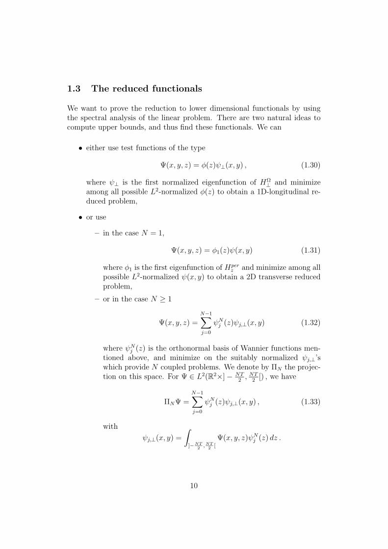
1.3 The reduced functionals
We want to prove the reduction to lower dimensional functionals by usingthe spectral analysis of the linear problem. There are two natural ideas tocompute upper bounds, and thus find these functionals. We can
• either use test functions of the type
Ψ(x, y, z) = φ(z)ψ⊥(x, y) , (1.30)
where ψ⊥ is the first normalized eigenfunction of HΩ⊥ and minimize
among all possible L2-normalized φ(z) to obtain a 1D-longitudinal re-duced problem,
• or use
– in the case N = 1,
Ψ(x, y, z) = φ1(z)ψ(x, y) (1.31)
where φ1 is the first eigenfunction of Hperz and minimize among all
possible L2-normalized ψ(x, y) to obtain a 2D transverse reducedproblem,
– or in the case N ≥ 1
Ψ(x, y, z) =N−1∑j=0
ψNj (z)ψj,⊥(x, y) (1.32)
where ψNj (z) is the orthonormal basis of Wannier functions men-tioned above, and minimize on the suitably normalized ψj,⊥’swhich provide N coupled problems. We denote by ΠN the projec-tion on this space. For Ψ ∈ L2(R2×]− NT
2, NT
2[) , we have
ΠNΨ =N−1∑j=0
ψNj (z)ψj,⊥(x, y) , (1.33)
with
ψj,⊥(x, y) =
∫
]−NT2,NT
2[
Ψ(x, y, z)ψNj (z) dz .
10

Computing the energy of a test function of type (1.30), we get
Qper,NΩ (Ψ) = ω⊥ + ENA (φ) (1.34)
where ENA is the functional on the NT -periodic functions in the z direction,defined on H1(R/NTZ) by
φ 7→ ENA (φ) =
∫ NT2
−NT2
(1
2|φ′(z)|2 +Wε(z)|φ(z)|2 + g |φ(z)|4
)dz (1.35)
with
g := g
(∫
R2
|ψ⊥(x, y)|4 dxdy)
=1
2πgω⊥. (1.36)
The functional ENA is introduced by [KMPS] who analyze a particular case.Its study in the small ε limit is one of the aims of this paper.
For test functions of type (1.31), we get in the case N = 1
QperΩ (Ψ) = λ1,z + EB,Ω(ψ) (1.37)
with
EB,Ω(ψ)
:=
∫
R2x,y
(1
2|∇x,yψ − iΩ× rψ|2 − 1
2Ω2r2|ψ|2 +
1
2ω2⊥(x2 + y2)|ψ|2 + g|ψ|4
)dx dy ,
(1.38)
and
g := g
(∫ T2
−T2
|φ1(z)|4 dz). (1.39)
In the case N > 1, we define ENB,Ω((ψj,⊥)j=0,...,N−1) by
Qper,NΩ (Ψ) := λ1,z
∑j
||ψj,⊥||2 + ENB,Ω((ψj,⊥)) (1.40)
with
Ψ =N−1∑j=0
ψNj (z)ψj,⊥(x, y) . (1.41)
Of course when minimizing over normalized Ψ’s, one gets more simply theproblem of minimizing
Qper,NΩ (Ψ) = λ1,z + ENB,Ω((ψj,⊥)) . (1.42)
11

As such, the energy ENB,Ω does not provide N coupled problems but onesingle energy depending on N test functions. Nevertheless, in the small εlimit, the Wannier functions are localized in each well. Thus each functionψj,⊥ only interacts with its nearest neighbors and this simplification pro-vides N coupled problems, as suggested by Snoek [Sn] on the basis of formalcomputations. We will analyze their validity. This reduced functional issomehow related to the Lawrence-Doniach model for superconductors (see[ABB1, ABB2]).
1.4 Main results
1.4.1 Universal estimates and applications
The analysis of the linear case immediately leads to the following trivialand universal inequalities (which are valid for any N and any Ω such that0 ≤ Ω < ω⊥)
λ1,z + ω⊥ ≤ Eper,NΩ ≤ λ1,z + ω⊥ + IN , (1.43)
where
IN :=gω⊥2Nπ
(∫ T2
−T2
|φ1(z)|4dz)
=I
N. (1.44)
This universal estimate is obtained by using the test function
Ψper,N(x, y, z) = ψ⊥(x, y)φN1 (z) ,
where φN1 is the N -th normalized ground state introduced in (1.26) andψ⊥(x, y) is the ground state of HΩ
⊥, actually independent of Ω.From (1.26), we have :
∫ NT2
−NT2
(φN1 (z))4 dz =1
N2
∫ NT2
−NT2
φ1(z)4 dz =
1
N
∫ T2
−T2
φ1(z)4 dz , (1.45)
where, as ε→ 0, and, under Assumption (1.7), it can be proved (see (3.10))that ∫ T
2
−T2
φ1(z)4 dz ∼ c4 ε
− 12 , (1.46)
for some explicitly computable constant c4 > 0.Thus, we have the following estimate for IN
IN ∼ c42π
gω⊥N
ε−12 . (1.47)
12

An immediate analysis shows that λ1,z + ω⊥ is a good asymptotic of
Eper,NΩ in the limit ε → 0 when g is sufficiently small (what we can call the
quasi-linear situation). More precisely, we have
Theorem 1.2.Under the condition that either
(QLa) g << ε12 , (1.48)
or(QLb) gω⊥ε
12 << 1 , (1.49)
then we haveEper,N
Ω = (λ1,z + ω⊥) (1 + o(1)) , (1.50)
as ε tends to 0.
Each of these conditions implies indeed that IN is small relatively to λzor to ω⊥.
So our goal is
• to have more accurate estimates than (1.50),
• to analyze more interesting cases when none of these two conditions issatisfied and to give natural sufficient conditions allowing the analysisof reduced models.
We are able to justify the reductions to the lower dimensional functionalsENA and ENB,Ω when their infimum is much smaller than the gap between thefirst two excited states of the linear problem in the other direction, namelyin case A, when mN
A is much smaller than δ⊥, where
mNA = inf
||φ||=1ENA (φ) , (1.51)
and in case B, when mNB,Ω is much smaller than 1/ε, the gap between the two
first bands of the periodic problem on the line, where
mNB,Ω = infP
j ||ψj,⊥||2=1ENB,Ω((ψj,⊥)) . (1.52)
An independent difficulty is then to have more accurate estimates mNA and
mNB,Ω according to the regime of parameters. We do not have universal esti-
mates for this but have to separate two cases :
13

• the Weak Interaction case, where the interaction term (L4 term) is atmost of the same order as the ground state of the linear problem in thesame direction;
• the Thomas Fermi case, where the kinetic energy term is much smallerthan the potential and interaction terms.
In what follows, when N is not mentioned in mNA , mN
B,Ω, ENA , ENB,Ω, thenthe notations are for N = 1. Similarly, if Ω is not mentioned, this meansthat either the considered quantity is independent of Ω or that we are treat-ing the case Ω = 0. To mention the dependence on other parameters, wewill sometimes explictly write this dependence like for example mN
A (ε, g) ormNB,Ω(g, ω⊥) .
1.4.2 Case (A) : the longitudinal model
We consider states which are of type (1.30) with ϕ ∈ L2(Rz/(NT )Z). Theenergy of such test functions provides the upper bound
Eper,NΩ ≤ ω⊥ +mN
A (ε, g) (1.53)
where mNA is given by (1.51) and g was introduced in (1.36).
In order to show that the upper bound is an approximate lower bound,we first address the “Weak Interaction” case,
(AWIa) 1 << ε(ω⊥ − Ω) , (1.54)
and, for a given c > 0,(AWIb) gω⊥ε
12 ≤ c . (1.55)
The first assumption implies that the lowest eigenvalue λ1,z of the linearproblem in the z direction (having in mind (1.24)) is much smaller than thegap in the transverse direction δ⊥ = ω⊥ − Ω. This will allow the projectiononto the subspace ψ⊥⊗L2(Rz/(NT )Z). The second assumption implies thatthe nonlinear term (of order gω⊥/
√ε) is of the same order as λ1,z. It implies
using (1.24), (1.47) and the universal estimate
λ1,z ≤ mNA ≤ λ1,z + IN , (1.56)
that
mNA ≈
1
ε. (1.57)
14

Here ≈ means “of the same order” in the considered regime of parameters.More precisely we mean by writing (1.57) that, for any ε0 > 0, there existsC > 0 such that, for all ε ∈]0, ε0], any g, ω⊥ satisfying (1.55),
1
Cε≤ mN
A ≤C
ε.
Note that most of the time, we will not control the constant with respect toN .All these rough estimates are obtained by rather elementary semi-classicalmethods which are recalled in Section 3. More precise asymptotics of mN
A
will be given under the additional Assumption (1.48) in Section 5.2. Thus,by (1.54), mN
A is much smaller than δ⊥. We will prove
Theorem 1.3.When ε tends to 0, and under Conditions (1.54) and (1.55), we have
Eper,NΩ = ω⊥ +mN
A (ε, g) (1 + o(1)) . (1.58)
We now describe the “Thomas-Fermi” regime, where we can also justify thereduction to the longitudinal model. We assume that, for some given c > 0 ,
(ATFa) gω⊥√ε >> 1 , (1.59)
(ATFb) gω⊥ε2 ≤ c , (1.60)
(ATFc) g512 ε−
16ω⊥
512 << (ω⊥ − Ω)
38 . (1.61)
Note that (1.59) is the converse of (1.55) while (1.59) and (1.61) imply that1 << ε(ω⊥ − Ω). This implies λ1,z << δ⊥, which is the main condition toreduce to case A. Assumptions (1.59) and (1.60) allow to show that :
mNA ≈
(gω⊥ε
) 23, (1.62)
and this also implies that the nonlinear term is much bigger than δz.The estimate (1.62) will be shown in Section 5.3, together with more preciseones with stronger hypotheses (see Assumption (5.19) and (5.20)).
Theorem 1.4.When ε tends to 0, and under Conditions (1.59), (1.60) and (1.61), we have,as ε→ 0,
Eper,NΩ = ω⊥ +mN
A (ε, g) (1 + o(1)) . (1.63)
The proofs give actually much stronger results.
15

1.4.3 Case (B) : the transverse model
This corresponds to the idea of a reduction on the ground eigenspace in thez variable, where the interaction term is kept in the transverse problem:therefore, this is a regime where ω⊥ε << 1. We recall that we denote by λ1,z
the (N -independent) ground state energy of Hper,Nz and by φN1 the normalized
ground state. We consider states which are of type (1.31) or (1.32). We havedefined ENB,Ω by (1.40)-(1.41) and mN
B,Ω, the infimum of the energy of suchtest functions by (1.52). We have the upper bound
Eper,NΩ ≤ λ1,z +mN
B,Ω . (1.64)
When N = 1, mB,Ω is a function of g and ω⊥ as it is clear from (1.38) and(1.52). Note that, from (1.46), we get
g = g(
∫ T2
−T2
φ1(z)4dz) ≈ g√
ε. (1.65)
Again we can discuss two different cases according to the size of the interac-tion. In the Weak Interaction case, we prove the following :
Theorem 1.5.When ε tends to 0, and under the conditions
(BWIa) gε−12 ≤ C , (1.66)
(BWIb) ω⊥ε << 1 , (1.67)
thenEper,N
Ω = λ1,z +mNB,Ω(1 + o(1)) . (1.68)
Condition (BWIb) implies that the bottom of the spectrum of the linearproblem in the x − y direction is much smaller than δz, the gap in the zdirection, which is of order 1/ε. Condition (1.66), together with (1.43) and(1.47), implies that mN
B,Ω satisfies
mNB,Ω ≈ ω⊥ . (1.69)
Indeed, (BWIa) and (BWIb) imply gε12ω⊥ << 1, that is (QLb).
In the Thomas-Fermi case, we prove the following :
16

Theorem 1.6.When ε tends to 0, and under the conditions
(BTFa)√ε << g , (1.70)
(BTFb) ω⊥√gε
34 << 1 , (1.71)
and(BTFc) g
32 ε
14ω⊥ << 1 , (1.72)
thenEper,N
Ω = λ1,z +mNB,Ω(1 + o(1)) . (1.73)
Note that (BTFa) is the converse of (BWIa). We will see in Proposition6.3 (together with (6.4), (6.16) and (6.49)) that, under these assumptionsand Assumption (6.15), the term mN
B,Ω satisfies
mNB,Ω ≈ ω⊥
√g/ε1/4 , (1.74)
and thus is much smaller than δNz which is of order 1ε.
Our proofs are made up of two parts : rough or accurate estimates ofmNA,Ω and mN
B,Ω on the one hand and a lower bound for Eper,NΩ on the other
hand. The lower bound consists in showing that the upperbound obtained byprojecting on the special states introduced above in (1.30), (1.31) or (1.32)is actually also asymptotically a good lower bound.
1.4.4 Tunneling effect and discrete model
Since the Wannier functions are localized in the z variable, the energy ofa function Ψ =
∑N−1j=0 ψNj (z)ψj,⊥(x, y) provides at leading order the sum of
N decoupled energies for ψj,⊥ on each slice j. At the next order, in thecomputation of the L2 norm of the gradient, only the nearest neighbors in zinteract through an exponentially small term, describing what is called thetunneling effect. These simplifications are discussed in section 7. We arelead to new functionals and in particular a discrete model that we analyzein relationship with the physics papers.
In case A, the behavior on each slice j is the same, given by ψ⊥ and it isthe behavior on the z direction which has a tunneling contribution. Thereare no vortices whatever the velocity Ω.
In case B, for N = 1, there are vortices for large velocity and they arelocated on each slice at the same place. For N large, it is an open and
17

interesting question to analyze whether it is possible for a vortex line to varylocation according to the slice, whether vortices interact between the slicesand how. This could be performed using our reduced models.
1.5 Organization of the paper
The paper is organized as follows. In Section 2, we start the spectral analysisof the linear problems in the longitudinal and transverse directions. We recallin particular the main techniques which can be used for the analysis of thespectral problem with periodic potential on the line. Section 3 is devoted tothe semi-classical results for the periodic problem. Although we are mainlyinterested in 1D-problems we recall here techniques which are true in anydimension and can be useful for the analysis of 2D or 3D optical lattices.
In Section 4, we prove the main theorems for case A. In Section 5, weanalyze the ground state of the 1D nonlinear energy ENA for N = 1 andN > 1 and also distinguish between the two cases: Weak Interaction andThomas-Fermi. Section 6 corresponds to a similar analysis for the transversemodels ENB . Section 7 is devoted to the tunneling effects and discuss, on thebasis of the semi-classical estimates of Section 3, some results by physicistson the discrete nonlinear Schrodinger model. In Section 8, we analyze variousboundary conditions and compare in particular the problems on R3 (whichis completely solved) and the problems on R2×] − NT
2, NT
2[ with periodic
condition which seem physically more interesting.
2 Analysis of the linear model
The linear model which appears naturally is associated to
HΩ = HΩ⊥ +Hz ,
which was presented in the introduction (see (1.17)-(1.21)). A natural con-dition (for the strict positivity of the operator HΩ
⊥) is Condition (1.5). Inthis situation with separate variables, we can split the spectral analysis inthe separate spectral analysis of HΩ
⊥ and the spectral analysis of a suitablerealization of Hz which will be presented in the next subsection.
18

2.1 The harmonic oscillator in the transverse variable
For simplicity, we begin the analysis of H⊥ = HΩ⊥ with the case Ω = 0.
The first operator HΩ=0⊥ is a harmonic oscillator with discrete spectrum and
the bottom of its spectrum is given by
inf(σ(H0⊥)) = ω⊥ . (2.1)
A corresponding L2-normalized ground state is the Gaussian
ψ⊥ =(ω⊥π
) 12exp−ω⊥
2r2 . (2.2)
Moreover the gap between the ground state energy and the second eigenvalue(which has multiplicity 2) is given by
λ2,⊥ − ω⊥ = ω⊥ . (2.3)
The spectrum of HΩ⊥ can be recovered by considering first the joint spec-
trum of HΩ⊥ and Lz. For each eigenspace of Lz corresponding to ` for some
` ∈ Z, we can look at the operator
H(`)⊥ := −1
2∆x,y +
1
2ω⊥2r2 − Ω` , (2.4)
considered as an unbounded operator on L2(R2) ∩ Ker (Lz − `).
More precisely, for Ω satisfying (1.5), a common eigenbasis of Lz and H0⊥
is given by the set of (not normalized) Hermite functions:
φj,k(x, y) = eω⊥2
(x2+y2) (∂x + i∂y)j (∂x − i∂y)
k(e−ω⊥(x2+y2)
)(2.5)
where j and k are non-negative integers.The eigenvalues are (j − k) for Lz and
Ej,k = ω⊥ + (ω⊥ − Ω)j + (ω⊥ + Ω)k (2.6)
for HΩ⊥.
The spectrum of H(`)⊥ is obtained by considering the pairs (j, k) such that
j − k = `.We emphasize that this orthogonal basis of eigenfunctions is independent ofΩ.
19
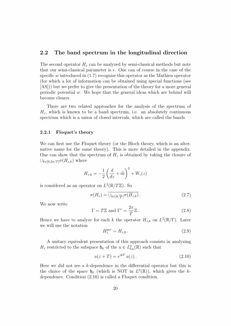
2.2 The band spectrum in the longitudinal direction
The second operator Hz can be analyzed by semi-classical methods but notethat our semi-classical parameter is ε. One can of course in the case of thespecific w introduced in (1.7) recognize this operator as the Mathieu operator(for which a lot of information can be obtained using special functions (see[AS])) but we prefer to give the presentation of the theory for a more generalperiodic potential w. We hope that the general ideas which are behind willbecome clearer.
There are two related approaches for the analysis of the spectrum ofHz, which is known to be a band spectrum, i.e. an absolutely continuousspectrum which is a union of closed intervals, which are called the bands.
2.2.1 Floquet’s theory
We can first use the Floquet theory (or the Bloch theory, which is an alter-native name for the same theory). This is more detailed in the appendix.One can show that the spectrum of Hz is obtained by taking the closure of∪k∈[0,2π/T ]σ(Hz,k) where
Hz,k = −1
2
(d
dz+ ik
)2
+Wε(z)
is considered as an operator on L2(R/TZ). So
σ(Hz) = ∪k∈[0, 2πT
]σ(Hz,k) . (2.7)
We now write
Γ = TZ and Γ∗ =2π
TZ . (2.8)
Hence we have to analyze for each k the operator Hz,k on L2(R/Γ). Laterwe will use the notation
Hperz = Hz,0 . (2.9)
A unitary equivalent presentation of this approach consists in analyzingHz restricted to the subspace hk of the u ∈ L2
loc(R) such that
u(z + T ) = eikT u(z) . (2.10)
Here we did not see a k-dependence in the differential operator but this isthe choice of the space hk (which is NOT in L2(R)), which gives the k-dependence. Condition (2.10) is called a Floquet condition.
20

This means that we have written, using the language of the Hilbertian-integrals, the decomposition
L2(R) =
∫ ⊕
[0,2π/T ]
hk dk (2.11)
and that we have for the operator the corresponding decomposition
Hz =
∫ ⊕
[0,2π/T ]
Hz,k dk , (2.12)
with Hz,k unitary equivalent to Hz,k.
For each k ∈ [0, 2π/T [, Hz,k has a discrete spectrum which can be de-scribed by an increasing sequence of eigenvalues (λj(k))j∈N. The spectrum ofHz is then a union of bands Bj, each band being described by the range of λj.At least when we have the additional symmetry Wε even, one can determinefor which value of k the ends of the band Bj are obtained. For j = 1, weknow in addition from the diamagnetic inequality that the minimum of λ1 isobtained for k = 0 :
infkλ1(k) = λ1(0) . (2.13)
2.2.2 Wannier’s approach
When the band is simple (and this will be the case for the lowest band inthe regime ε small), one can associate to λj(k) a normalized2 eigenfunctionϕj(z, k) with in addition an analyticity with respect to k together with the(2π/T )-periodicity in k.
In this case (we now take j = 1), one can associate to ϕ1, which satisfies,
ϕ1(z + T ; k) = ϕ1(z, k) , (2.14)
and
ϕ1(z; k +2π
T) = ϕ1(z, k) , (2.15)
a family of Wannier’s functions (ψ`)`∈Γ defined by
ψ0(z) =T
2π
∫ 2πT
0
exp(ikz) ϕ1(z, k) dk , ψ`(z) = ψ0(z − `) , (2.16)
2in L2(]− T2 ,
T2 [),
21

for ` ∈ Γ .In addition, we can take ψ0 real. One can indeed construct ϕ1 satisfying inaddition the condition
ϕ1(z, k) = ϕ1(z,−k) . (2.17)
One obtains (after some normalization of ψ0) that
Proposition 2.1.
(i) The family (ψ`)`∈Γ gives an orthonormal basis of the spectral space at-tached to the first band.
(ii) ψ0 is an exponentially decreasing function.
The second point can be proved using the analyticity3 with respect to k.This orthonormal basis corresponding to the first band plays the role of the
basis Pj(z) exp− |z2|2
in the Lowest Landau Level approximation.Note that we recover ϕ1(z, k) by the formula
ϕ1(z, k) = exp(−ikz)∑
`∈Γ
exp(ik`) ψ`(z) . (2.18)
Moreover, the operator A on `2(Γ) whose matrix is given by
A``′ = 〈Hzψ`, ψ`′〉 (2.19)
is unitary equivalent to the restriction of Hz to the spectral space attachedto the first band.One can of course observe that A commutes with the translation on `2(Γ),so it is a convolution operator by a sequence a ∈ `1(Γ) (actually in the spaceof the rapidly decreasing sequences S(Γ)),
A``′ = a(`− `′) , (2.20)
which is actually the Fourier series of k 7→ λ1(k)
λ1 = a , (2.21)
where
λ1(`) :=T
2π
∫ 2π/T
0
exp(−i`k) λ1(k) dk . (2.22)
So we have(Au)(`) =
∑
`′∈Γ
a(`− `′)u(`′) , for u ∈ `2(Γ) .
3One can make a contour deformation in the integral defining ψ0 in (2.16).
22

2.2.3 (NT )-periodic problem
There is another way to proceed at least heuristically. We keep w T -periodicbut look at the (NT )-periodic problem and we analyze this problem. Thespectrum is discrete but the idea is that we will recover the band spectrumin the limit N → +∞. If we compare with what we do in the Floquettheory, the analysis of the (NT )-periodic problem consists in consideringthe direct sum of the problems with a Floquet condition corresponding tok = 0, 2π
NT, · · · , 2π(N−1)
NT.
Note that this decomposition into a direct sum works only for linearproblems, so it will be interesting to explore this approach for the non linearproblem.
In this spirit, it can be useful to have an adapted orthonormal basis ofthe spectral space attached to the first N eigenvalues of the NT -periodicproblem (which can be identified with the vector space generated by theeigenfunctions corresponding to the N Floquet eigenvalues associated withk = 0, 2π
NT, · · · , 2π(N−1)
NT.
Our claim is that there exists an orthonormal basis, for the L2-norm on]− NT
2, NT
2[, consisting of (NT )-periodic functions and replacing the Wannier
functions.
We write
ψN0 (z) =1√N
N∑j=1
φNj (z) , (2.23)
where φNj is an eigenfunction4 of the (NT )-periodic problem, chosen in sucha way that
φNj (z + T ) = ωj−1N φNj (z) , (2.24)
with ωN = exp(2iπ/N).We can then introduce
ΓN = Γ/(NTZ) , (2.25)
and define, for ` ∈ ΓN = Γ, the (NT )-Wannier functions
ψN` (z) = ψN0 (z − `) (2.26)
4Note that except in the case j = 1, we do not claim that φNj is the j-th eigenfunction
but this is the first one corresponding to the condition (2.24).
23

This gives an orthonormal basis of the eigenspace attached to the first Neigenvalues of the (NT )-periodic problem. These first N eigenvalues belongto the previously defined first band.
Note that conversely, we can recover the eigenfunctions φNj from the ψNjby a discrete Fourier transfrom. In particular we have
φN1 =1√N
N−1∑j=0
ψNj . (2.27)
Except the fact that these “Wannier” functions are NOT exponentiallydecreasing at ∞ (they are by construction (NT )-periodic), one can thenplay with them in the same way (this corresponds to the replacement of theFourier series by the finite dimensional one). We then meet the “discreteconvolution” on `2(ΓN) :
(ANu)(`) =∑
`′∈ΓN
aN(`− `′)u(`′) , for u ∈ `2(ΓN) .
Of course `2(ΓN) is nothing else than CN with its natural Hermitian struc-ture.
We have presented different techniques to determine the bottom of thespectrum ofHz, which all provide the same ground energy. We will now recallmore quantitative results based on the so-called semi-classical analysis.
3 Semi-classical analysis for the T -periodic
case
3.1 Preliminary discussion
Till now, we have not strongly used that we are in a semi-classical regime:our semi-classical parameter here will not be the Planck constant ~ (whichwas already assumed to be equal to 1) but ε. We will now use this additionalassumption for extracting quantitative results from the previously presentedqualitative theory. As already said, the physics literature is analyzing a veryparticular model, the Mathieu equation. We will rapidly sketch how one cando this in full generality. For the one dimensional case which is considered
24

here, one can probably refer to Harrell [Ha] (who uses techniques of ordinarydifferential equations) or to the book of Eastham [Eas], but we will describea proof which is more general in spirit, which is not limited to the one dimen-sional situation (see Simon [Si], Helffer-Sjostrand [HeSj1], Outassourt [Ou])and is described in the books of Helffer [He] or Dimassi-Sjostrand [DiSj].As we have shown in the previous section, the good description of the firstband, can be either obtained by a good approximation of λ1(k) and ϕ1(z, k)as ε → 0 or by first finding a good approximation of the Wannier functionψ0 introduced in (2.16), which is expected to be exponentially localized inone well, or of the (NT )-periodic Wannier function introduced in (2.23).
The analysis is done usually in two steps. First we localize roughly λ1(k),then we analyze very accurately the variation of λ1(k)− λ1(0).The first one will be obtained by a harmonic approximation and the secondone by the analysis of the tunneling effect.
3.2 The harmonic approximation
We will provide the explanation in a general case containing the model con-sidered by Snoek [Sn] as a particular case. We recall that we work underAssumption 1.1. The statements below are sometimes written vaguely andwe refer to [DiSj] or [He] for more precise mathematical statements.For the approximation of λ1,z(0) (actually for any λ1,z(k)) the rule is thatwe replace w(z) (having in mind (1.7)) by its quadratic approximation at 0.The harmonic approximation consists in first looking at the operator
−1
2
d2
dz2+
w′′(0)
2ε2z2 , (3.1)
on R.For the model in [Sn], w(z) = sin2(πz
T), and we find
−1
2
d2
dz2+
1
ε2(πz
T)2 . (3.2)
This operator is a harmonic oscillator whose spectrum is explicitly known.The j-th eigenvalue is given by
λharj,z =j − 1
2
ε
√w′′(0) . (3.3)
25
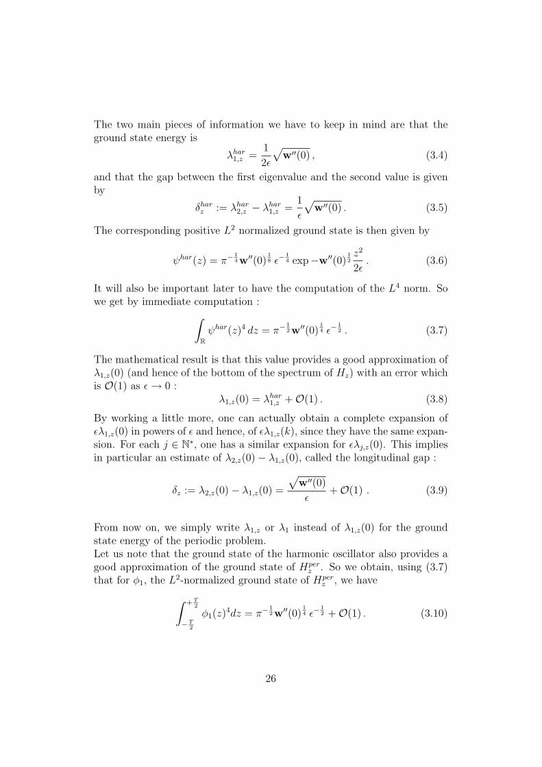
The two main pieces of information we have to keep in mind are that theground state energy is
λhar1,z =1
2ε
√w′′(0) , (3.4)
and that the gap between the first eigenvalue and the second value is givenby
δharz := λhar2,z − λhar1,z =1
ε
√w′′(0) . (3.5)
The corresponding positive L2 normalized ground state is then given by
ψhar(z) = π−14w′′(0)
18 ε−
14 exp−w′′(0)
12z2
2ε. (3.6)
It will also be important later to have the computation of the L4 norm. Sowe get by immediate computation :
∫
Rψhar(z)4 dz = π−
12w′′(0)
14 ε−
12 . (3.7)
The mathematical result is that this value provides a good approximation ofλ1,z(0) (and hence of the bottom of the spectrum of Hz) with an error whichis O(1) as ε→ 0 :
λ1,z(0) = λhar1,z +O(1) . (3.8)
By working a little more, one can actually obtain a complete expansion ofελ1,z(0) in powers of ε and hence, of ελ1,z(k), since they have the same expan-sion. For each j ∈ N∗, one has a similar expansion for ελj,z(0). This impliesin particular an estimate of λ2,z(0)− λ1,z(0), called the longitudinal gap :
δz := λ2,z(0)− λ1,z(0) =
√w′′(0)
ε+O(1) . (3.9)
From now on, we simply write λ1,z or λ1 instead of λ1,z(0) for the groundstate energy of the periodic problem.Let us note that the ground state of the harmonic oscillator also provides agood approximation of the ground state of Hper
z . So we obtain, using (3.7)that for φ1, the L2-normalized ground state of Hper
z , we have
∫ +T2
−T2
φ1(z)4dz = π−
12w′′(0)
14 ε−
12 +O(1) . (3.10)
26

3.3 The tunneling effect
We now briefly explain the results about the length of the first band, whichis exponentially small as ε → 0. The results can take the following form(see the work of Outassourt [Ou] or the book by Dimassi-Sjostrand, Formula(6.26))
λ1(k)− λ1(0) = 2(1− cos(kT ))τ +O(exp−S + α
ε) (3.11)
with α > 0 (arbitrarily close from below to 1) and, for some cτ 6= 0,
τ ∼ cτ ε− 3
2 exp−Sε. (3.12)
Moreover one can express the constants cτ and S once w is given (see5 also[He] in addition to the previous references). This τ seems to be called insome physical literature the hopping amplitude.Here, we simply explain how one computes S which determines the exponen-tial decay of τ as ε → 0. In any dimension, S is interpreted as the minimalAgmon distance between two different minima of the potential w. In onedimension, with w satisfying Assumption (1.1), this distance is simply theAgmon distance between two consecutive minima and is given by
S :=√
2
∫ T2
−T2
√w(z) dz . (3.13)
In particular, when w(z) = sin2(πzT
), we get
S :=√
2
∫ T2
−T2
| sin(πz
T)| dz =
2√
2T
π. (3.14)
This is to compare to (14) in [SnSt1], which is not an exact formula (aswrongly claimed) but only an asymptotically correct formula. It can befound, for this Mathieu operator, in [AS].Let us give the formula for the constant cτ . It can be found in [Ha], see also[Ou], Formula (4.14) and [He] p. 58-59. We have :
cτ = 234π−
12 expAτ , (3.15)
with (assuming w even)
Aτ = limη→0
(∫ T2
η
1√w(z)
dz +
√2√
w′′(0)ln η
). (3.16)
5The computation is a little simpler in the case when w is even.
27

We just sketch the mathematical proof. Filling out all the wells suitablyexcept one (say 0), we get a new potential wmod ≥ w which coincides with win an interval containing 0 and excluding small neighborhoods of all the otherminima. We consider, for ε small enough, the ground state of this modifiedproblem and (multiplying by a cut-off function) we get a function ψapp0 (andan eigenvalue λapp1 ) which is a very good approximation of ψ0.Now the hopping amplitude in the abstract theory is given6 exactly by
−τ = a(T ) = 〈Hzψ0 , ψ1〉 = 〈(Hz − µ)ψ0 , ψ1〉 , (3.17)
the last equality being satisfied, due to the orthogonality of ψ0 and ψ1, for anyµ. When replacing ψ0 by its approximation, one has to be careful, becauseψapp0 and ψapp1 := ψapp0 (· − T ) are no more orthogonal. So this leads to takeµ = λapp1 , and one can prove that
τ ∼ −〈(Hz − λapp1 )ψapp0 , ψapp1 〉 . (3.18)
An easy way to see that τ is exponentially small is to observe that
〈(Hz − λapp1 )ψapp0 , ψapp1 〉 = ε−2 〈(w(z)− wmod)ψapp0 , ψapp1 〉 , (3.19)
and to use the information on the asymptotic decay of ψapp0 . The WKB-approximation of ψapp0 is, in a neighborhood of 0,
ψwkb0 = ε−14 b(z, ε) exp−1
ε
∫ z
0
√w(s)ds , for z ≥ 0 , (3.20)
withb(z, ε) ∼
∑j≥0
bj(z)εj , (3.21)
and
b0(z) = π−14 exp
−
∫ z
0
(w12 )′(t)−
√w′′(0)
2
2√
w(t)dt
. (3.22)
It should then be completed by symmetry to get an even WKB solution on]− T,+T [.Note that we have
(w12 )′(T−) = −
√w′′(0)
2,
which implies that b0 tends to +∞ as z → T−.
6For the Mathieu potential, this is consistent with Formula (13) in [SnSt1].
28

An integration by parts together with a WKB approximation leads to theasymptotic estimate of τ announced in (3.12). More precisely, we get that
the prefactor cτ is immediately related to the constant b0(T2)2
√V (T
2) and
this leads to (3.15). Note that more generally we have
b0(z)b0(T − z)√V (z) = Cst , (3.23)
which again shows the blowing up of b0 at T .
Finally, we emphasize that ψwkb0 is a good approximation of ψ0 only inintervals ]− T + η, T − η[ for some η > 0.
One can also see that a(kT ) is of the order of |a(T )||k| (for k ≥ 2)
a(kT ) = O(τ 2) , (3.24)
so it is legitimate in order to compute the width of the first band to forgetall the a(`) for ` ∈ Γ, ` 6= 0,±T .Thus, in the k variable, the spectrum (corresponding to the first band) is upto a very small error, of the order of the square of a(T ), given by the operatorof multiplication in L2(R/Γ) by the function a(0) + 2a(T ) cos(kT ).
Remark 3.1.What is written above corresponds to the use of Wannier functions on R. Onecan write a close theory using the (NT )-periodic Wannier functions withoutmodifying the main terms of the asymptotics. In particular, ψwkb0 is also agood approximation of ψN0 in intervals ]− T + η, T − η[ for some η > 0.The interest of the Wannier functions on R is that they allow to recover theinformation for all Floquet eigenvalues (see the discussion in Section 7.1).
4 Justification of the reduction to the longi-
tudinal energy ENA4.1 Main result
In this section, we address the reduction to the energy ENA defined in (1.35)and prove the following theorem (recall that mN
A is defined in (1.51)):
29

Theorem 4.1. If
(AΩa) mNA (ε, g)(ω⊥ − Ω)−1 << 1 (4.1)
and(AΩb) g(2ω⊥ − Ω)mN
A (ε, g)(ω⊥ − Ω)−32 << 1, (4.2)
we haveinf
||Ψ||=1Eper,NΩ (Ψ) = ω⊥ +mN
A (ε, g)(1 + o(1)). (4.3)
Both Theorem 1.3 and Theorem 1.4 are a consequence of Theorem 4.1 assoon as we have the appropriate rough estimates on mN
A already presentedin the introduction. This is what we explain first in Subsection 4.2 beforeproving the theorem in Subsection 4.3.
4.2 Proof of Theorem 1.3 and Theorem 1.4
4.2.1 Weak Interaction case
In the Weak Interaction case, we recall from (1.57), that, when (1.55) issatisfied, then
mNA ≈ 1/ε . (4.4)
Therefore, when (1.54) and (1.55) are satisfied, then (4.1) and (4.2) auto-matically hold with the observation that
g(2ω⊥ − Ω)(ω⊥ − Ω)−32mN
A (ε, g) ≤ Cg(2ω⊥ − Ω)ε12 ((ω⊥ − Ω)ε)−
32 << 1 ,
and Theorem 1.3 follows from Theorem 4.1.
4.2.2 Thomas-Fermi case
In the Thomas-Fermi case, we will prove in (5.18) that, when (1.59) and(1.60) are satisfied, then
mNA ≈ (gω⊥/ε)2/3 . (4.5)
Let us verify that, if (1.59), (1.60) and (1.61) are satisfied, then (4.1) and(4.2) hold. This will prove Theorem 1.4.
We get (4.1) in the following way. First we have :
(ω⊥ − Ω)−1mNA (ε, g) ≤ C(ω⊥ − Ω)−1ω⊥
23 g
23 ε−
23 .
30

Hence (4.1) is a consequence of
gω⊥ << ε(ω⊥ − Ω)32 , (4.6)
which follows from (1.61) since (1.59) and (1.61) imply that (ω⊥−Ω)ε >> 1.The check of (4.2) is then immediate from (1.61) and (4.5).
4.3 Proof of Theorem 4.1
Because of the upper bound (1.53), Theorem 4.1 is a consequence of thefollowing proposition, recalling that δ⊥ = ω⊥ − Ω .
Proposition 4.2.There exists a constant C > 0 such that, for all ε ∈]0, 1], for all ω⊥, Ω s.t.δ⊥ ≥ 1 and for all g ≥ 0 ,
inf||Ψ||=1
Qper,NΩ (Ψ) = ω⊥ +mN
A (ε, g) (1− CrA(ε, g)) , (4.7)
with
0 ≤ rA(ε, g) ≤ g1/4δ− 1
8⊥
(δ⊥ + ω⊥δ⊥
) 14
mNA (ε, g)
14 + mA(ε, g)δ⊥
−1 . (4.8)
Proof of the propositionFor simplicity, we make the proof for Ω = 0. Note also that
1− CrA(ε, g) ≥ 0
by the lower bound. So we have only to prove (4.8) under the additionalcondition that the right hand side of (4.8) is less than some fixed α0 . In anycase, the estimate is only interesting in this case !The proof does not depend on N and for Ω not zero, we will make a remarkat the end on how to adapt it, using the diamagnetic inequality.
The proof is inspired by [AB] where a reduction is made from a 3D to a 2Dsetting for a fast rotation. We project a minimizer Ψ onto ψ⊥⊗L2(R/NTZ),and call ψ⊥(x, y) ξ(z) its projection:
Ψ(x, y, z) = ψ⊥(x, y)ξ(z) + w(x, y, z) with
∫
R2
ψ⊥(x, y)w(x, y, z) dxdy = 0 .
(4.9)
31

The orthogonality condition implies in particular
1 =
∫ NT2
−NT2
|ξ(z)|2 dz +
∫
R2×]−NT2,NT
2[
|w(x, y, z)|2 dxdydz (4.10)
and we have the lower bound∫ NT
2
−NT2
E ′B(w(·, ·, z)) dz ≥ (δ⊥+ω⊥)
∫
R2×]−NT2,NT
2[
|w(x, y, z)|2 dxdydz , (4.11)
with
E ′B(ψ) =
∫
R2
(1
2|∇x,yψ(x, y)|2 +
ω⊥2
2(x2 + y2) |ψ(x, y)|2
)dxdy .
We compute the energy of Ψ and use the orthogonality condition and theequation satisfied by ψ⊥ to find that all the cross terms disappear so that
QN,per(Ψ) = ω⊥
∫ NT2
−NT2
|ξ(z)|2 dz + EN ′A (ξ)
+
∫
R2
EN ′A (w(x, y, ·)) dxdy +
∫ NT2
−NT2
E ′B(w(·, ·, z)) dz
+ g
∫
R2×]−NT2,NT
2[
|Ψ(x, y, z)|4 dxdydz , (4.12)
where
EN ′A (φ) =
∫ NT2
−NT2
(1
2|φ′(z)|2 +Wε(z)|φ|2
)dz .
From (4.10), (4.11) and (4.12), we find
QN,per(Ψ) ≥ ω⊥ +δ⊥
δ⊥ + ω⊥
∫ NT2
−NT2
E ′B(w(·, ·, z)) dz +
∫
R2
EN ′A (w(x, y, ·)) dxdy .
(4.13)We use (4.13) together with the upper bound (1.53) and (4.11) to derive that
∫
R2×]−NT2,NT
2[
|w(x, y, z)|2 dxdydz ≤ mNA (ε, g)
δ⊥. (4.14)
Note that the righthand side in (4.14) is very small according to Conditions(4.1) and (4.2).Note that (4.14) implies
∫ NT2
−NT2
|ξ(z)|2dz ≥ 1− mNA (ε, g)
δ⊥. (4.15)
32
Then, we get also,
∫R2×]−NT
2,NT
2[|∇x,yw(x, y, z)|2 dxdydz ≤ 2 δ⊥+ω⊥
δ⊥mN
A (ε,bg)ω⊥
,∫R2×]−NT
2,NT
2[|∂zw(x, y, z)|2 dxdydz ≤ 2 mN
A (ε, g) .(4.16)
The proof of the Sobolev embedding of H1(R3) in L6(R3) gives (see for ex-ample [Bre], p. 164, line -1) for a general function v in H1(R3)
‖v‖6 ≤ 4‖∂xv‖1/32 ‖∂yv‖1/3
2 ‖∂zv‖1/32 . (4.17)
Here ‖ · ‖p denotes the norm in Lp(R3).In our case, we are working in H1(R2
x,y × (Rz/NTZ)). A partition of unityin the z variable allows us to extend this estimate also this case, and we get,for another universal constant C,
‖w‖6 ≤ CN‖∂xw‖1/32 ‖∂yw‖1/3
2
(‖∂zw‖22 + ||w||22
)1/6, (4.18)
where this time || · ||p denotes the norm in Lp(R2x,y×]− NT
2, NT
2[).
So we obtain :
‖w‖6 ≤ CmNA (ε, g)
12
(δ⊥ + ω⊥δ⊥
) 13
. (4.19)
(C, C are N -dependent constants possibly changing from line to line.)Since by Holder’s Inequality,
‖w‖4 ≤ ‖w‖1/42 ‖w‖3/4
6 ,
we deduce that
‖w‖4 ≤ C mA(ε, g)12 δ⊥
− 18
(δ⊥ + ω⊥δ⊥
) 14
. (4.20)
We expand
|Ψ|4 = |ψ⊥|4|ξ|4+2|ψ⊥|2|ξ|2|w|2+4(<(ψ⊥ξw)+1
2|w|2)2+4|ψ⊥|2|ξ|2<(ψ⊥ξw) .
Since (4.12) implies that
EN(Ψ) ≥ ω⊥ + ENA (ξ)− 4g
∫
R2×]−NT2,NT
2[
|ψ⊥(x, y)|3|ξ(z)|3|w(x, y, z)| dxdydz ,
33

in order to get the lower bound, we just need to prove that the last term isa perturbation to ENA (ξ).We can do the following estimates
g∫ |ψ⊥(x, y)|3|ξ(z)|3|w(x, y, z)| dxdydz
≤ c0gω⊥34 (
∫ |ψ⊥(x, y)|4 dxdy) 34 (
∫ |ξ(z)|4dz) 34 ‖w‖4
≤ c1g1/4(ENA (ξ))3/4‖w‖4
≤ c2g1/4δ⊥
− 18
(δ⊥+ω⊥δ⊥
) 14mNA (ε, g)
12 (ENA (ξ))3/4
≤ c3g1/4δ⊥
− 18
(δ⊥+ω⊥δ⊥
) 14mNA (ε, g)
14
(1 + C mN
A (ε, g)δ⊥−1
) ENA (ξ) .
Here to get the last line, we have used the lower bound
ENA (ξ) ≥ mNA (ε, g) ||ξ||42 ,
and (4.15).This leads to
EN(Ψ) ≥ ω⊥+ENA (ξ)
(1− C g1/4δ⊥
− 18
(δ⊥ + ω⊥δ⊥
) 14
mNA (ε, g)
14 − C mN
A (ε, g)δ⊥−1
),
and then to (4.7).
Remark 4.3.In the case with rotation Ω, the proof is the same if we replace E ′B by E ′B,Ωdefined by
E ′B,Ω(ψ) =
∫
R2
(1
2|∇x,yψ − iΩr⊥ψ|2 +
1
2(ω⊥2 − Ω2)r2|ψ|2
)dxdy . (4.21)
We also use the diamagnetic inequality
∫|∇|w|(x, y)|2 dxdy ≤
∫| (∇w − iΩr⊥w
)(x, y)|2 dxdy (4.22)
which provides the Sobolev injections.
Remark 4.4.Here, we have not proved that the minimizer of E behaves almost like theground state in x, y times a function of ξ which minimizes EA. We are justable (see (4.14)) to prove that the minimizer is close to its projection (insome L2 or L4 norm). When N = 1, this can be improved under the stronger
34

condition (1.49). We first observe (note that (4.13) is still true with theaddition of E ′A(ξ) on the right hand side) that
E ′A(ξ) ≤ mA(ε, g) . (4.23)
Using (4.15), assuming mA
δ⊥< 1, this leads to
E ′A(ξ) ≤ mA(ε, g)(1− mA(ε, g)
δ⊥)−1||ξ||2 (4.24)
We will show in Subsection 5.2 (see (5.14)) how to proceed in order to showthat ξ is close to the ground state φ1(z) of Hper
z .This can allow to improve the information given in Theorem 1.2.
5 The 1D periodic model : estimates for mNA
The aim of this section is to analyze mNA . We note that rough estimates
were already given for the weak interaction case which were enough for thejustification of the model but the corresponding rough estimates needed forthe Thomas-Fermi justification will be obtained in this section. We will thenlook at accurate estimates for mN
A , which will be established under strongerhypotheses. We will end the section by the discussion of the case N > 1,which finally leads to the introduction of the DNLS model for the WeakInteraction case.
5.1 Universal estimates
We consider the one dimensional situation and a T - periodic potential W ,which could be for example W (z) = (sin πz)2/ε2. We consider the problemof minimizing on L2(R/TR) the functional
ψ 7→ G(ψ) =1
2
∫ T2
−T2
|ψ′(z)|2 dz +
∫ T2
−T2
W (z)|ψ(z)|2 dz + g
∫ T2
−T2
|ψ(z)|4 dz ,(5.1)
over ||ψ||L2 = 1.We are interested in the control of the minimum of the functional and willsimply prove
35

Lemma 5.1.If g ≥ 0, then
m(g) := inf||ψ||L2=1
G(ψ) = λ1 + g
∫ +T2
−T2
|φ1(z)|4 dz + o(g) , (5.2)
where (λ1, φ1) is the spectral pair of −12d2
dz2+ W (z) corresponding to the
ground state energy (with ||φ1||2 = 1).
Proof :It is clear that
λ1 ≤ m(g) ≤ λ1 + g
∫ T2
−T2
|φ1(z)|4dz , (5.3)
so the question is now to improve the lower bound.One could of course think of applying bifurcation theory but this gives onlya local result and we need in any case a global estimate for showing that theglobal minimizer of G is closed to φ1 as g is small.Let φmin be a minimizer of G, then we know that
1
2
∫ T2
−T2
|φ′min|2dz +
∫ T2
−T2
W (z)|φmin(z)|2 dz ≤ λ1 + g
∫ T2
−T2
|φ1(z)|4 dz . (5.4)
So φmin plays the role of a quasimode (or approximate eigenfunction) for−1
2d2
dz2+W (z).
A rather standard theorem in perturbation theory (we can write φmin =αφ1 + u⊥), gives first
1− |α|2 = ||u⊥||2 ≤ g
∫ T2
−T2
|φ1(z)|4 dzλ2 − λ1
,
and then the existence of a complex number c of modulus 1 such that
||φmin − cφ1||2L2 ≤ 2g
∫ T2
−T2
|φ1(z)|4 dzλ2 − λ1
. (5.5)
Here λ2 denotes the second eigenvalue of or Hamiltonian.Of course, the estimate is only interesting if
2g
∫ T2
−T2
|φ1(z)|4 dzλ2 − λ1
< 1 . (5.6)
36

We can now write
m(g) ≥ λ1 + g∫ T
2
−T2
|φmin(z)|4 dz≥ λ1 + g
∫ T2
−T2
|φ1(z)|4 dz − 4g||φmin − cφ1||2||φ1||36 .(5.7)
For the last estimate, we develop |φmin|4 in the following way
|φmin|4 = |cφ1 + φmin − cφ1|4≥ |φ1|4 + 2|φ1|2|φmin − cφ1|2 − 4|φ1|3|φmin − cφ1| . (5.8)
From this inequality we get
|φmin|4 ≥ |φ1|4 − 4|φ1|3|φmin − cφ1| . (5.9)
It just remains to control ||φ1||6 uniformly with respect to g, which can bededuced of the uniform control of the norm of φ1 in L6.
One can actually be more precise on what we have claimed in Lemma 5.1.
Lemma 5.2.If g ≥ 0, then
m(g) ≥ λ1 + g||φ1||44 − 252 g
32 ||φ1||36||φ1||24(λ2 − λ1)
− 12 . (5.10)
This estimate is interesting if
g <1
32||φ1||44||φ1||−6
6 (λ2 − λ1) . (5.11)
Remark 5.3.Everything being universal, one can of course replace T by NT in the de-scription.
5.2 Semi-classical results in the Weak Interaction case :N = 1
We first recall that using (3.10) we have, under Condition (1.55), the roughcontrol
1
Cε≤ λ1,z ≤ mA(ε, g) ≤ λ1,z + g
∫ T2
−T2
|φ1(z)|4 dz ≤ C
ε, (5.12)
37

which leads to (1.57) for N = 1 and was sufficient for the justification of thelongitudinal model A.
Let us now show that under stronger assumptions one can have a moreaccurate asymptotics including the main contribution of the non-linear in-teraction.
Proposition 5.4.Under Assumption (1.49), mA admits the following asymptotics :
mA(ε, g) = λhar1 (ε) + π−12w′′(0)
14 gε−
12 + c0 +O(ε) +O(g
32 ε−
14 ) . (5.13)
Proof :Indeed, λ1 and λ1 − λ2 are of order 1
ε, and by (3.10) and (5.5), we get
||φmin − cφ1||2L2 ≤ Cgε12 . (5.14)
Using the harmonic approximation, the term ||φ1||6 is of order ε−16 and the
remainder appearing in (5.10) is of order g32 ε−
14 . Altogether we get for the
energy
mA(ε, g) = λ1,z + g
∫ T2
−T2
|φ1(z)|4 dz +O(g32 ε−
14 ) . (5.15)
Using (3.10), we obtain (5.13). This asymptotics becomes interesting in thesemi-classical regime if (1.49) holds.
Remark 5.5.Exponentially small effects will be discussed in Section 7.
5.3 Semi-classical analysis in a Thomas-Fermi regime :case N = 1.
5.3.1 Main results
In this subsection, we first give the rough estimate leading to (1.62) forN = 1.Recall that g = 1
πgω⊥, but g and ε are taken as independent parameters.
Proposition 5.6.If for some c > 0,
gε2 ≤ c , (5.16)
38

and ifgε
12 >> 1 , (5.17)
then there exist C and ε0 such that
1
Cg
23 ε−
23 ≤ mA(ε, g) ≤ Cg
23 ε−
23 , ∀ε ∈]0, ε0] . (5.18)
We will also get the following accurate estimate :
Proposition 5.7.If
gε2 << 1 , (5.19)
and (5.17) are satisfied , then
mA(ε, g) = 2−43 3
53 5−1w′′(0)
23 g
23 ε−
23
(1 +O(g−
23 ε−
13 )
). (5.20)
The new asusmption is (5.19), which is stronger than (5.16).
5.3.2 The harmonic functional on R
Let us start with the case of a harmonic potential Wε(z) = γ z2
2ε2on R, with
γ > 0, and consider the problem of minimizing
qHr,T (u) =1
2
∫ T2
−T2
u′(t)2 dt+γ
2ε2
∫ T2
−T2
t2u(t)2 dt+ g
∫ T2
−T2
u(t)4 dt (5.21)
over the u’s in the form domain of qHr,T such that ||u||2 = 1.We denote by mHr,T
A the infimum of the functional. Actually there are twoapproximating “ harmonic ” functionals of interest corresponding to T finiteand to T = +∞. An interesting point is that, for T large enough, theminimizers of these two functionals are the same as we will see below. Butlet us start with the case T = +∞.
Lemma 5.8.If (5.17) holds, then
mHr,+∞A (ε, g) = 2−
43 3
53 5−1γ
23 g
23 ε−
23
(1 +O(g−
23 ε−
13 )
). (5.22)
39

The proof is very standard (see for example [BBH], [Af] or [CorR-DY]which treat the (2D)-case). The analysis is done through a dilation. Welook for an L2-normalized test function φ in the form
φ(z) = ρ12v(ρz) , (5.23)
with ρ and v to be determined.The 1−D energy of φ becomes
1
2ρ2
∫
Rv′(t)2dt+ ρ−2ε−2
γ
∫
Rt2v(t)2dt+ gρ
∫
Rv(t)4dt , (5.24)
with
εγ = ε/
√1
2γ .
This leads to choose ρ = ργ such that
ρ−3 = gε2γ ,
henceργ = ε
− 23
γ g−13 , (5.25)
and the energy of this model becomes
g23 ε−
23
(qTF (v) +
1
2(ε
12γ g)
− 43
∫
Rv′(t)2 dt
)(5.26)
with
qTF (v) :=
∫
Rt2v(t)2 dt+
∫
Rv(t)4 dt . (5.27)
This is asymptotically of the order of g23 ε−
23 and Condition (5.17) is just
the condition that the kinetic term is negligeable in the computation of theenergy.Let us recall the details of this asymptotics for completeness. We have firstto minimize over L2-normalized v the approximating functional qTF . Theminimizer vmin(t) of qTF is determined by the equations
t2v(t) + 2v(t)3 = λv(t) ,
∫
Rv(t)2dt = 1 . (5.28)
We get
vmin(t) = 2−12 (λ− t2)
12+ , (5.29)
40

with
λ =
(3
2
) 23
, (5.30)
and for x ∈ R,(x)+ = max(x, 0) .
The corresponding TF-energy is
eTF :=
∫
R(t2vmin(t)
2 + vmin(t)4) dt =
2
5λ
52 . (5.31)
Unfortunately, this minimizer is not in H1(R) and can not be used directlyfor our initial rescaled functional
qσTF (v) = qTF (v) + σ
∫
Rv′(t)2 dt ,
withσ = g−
43 ε− 2
3γ .
Here we recall that (5.17) implies
0 ≤ σ << 1 .
So we need to regularize this minimizer to have an upperbound for the energyof our “harmonic” functional which is good as σ → 0.
This can be done in the following way (see for example [Af] and referencestherein).
We introduce
γ(s) =
√s , if s > σ
13
sσ−16 , if s < σ
13
(5.32)
Let us consider the function
vσ(t) = γ(vmin(t)2) .
We get that vσ belongs to H1 and satisfies
∫|vσ(t)|2 dt = 1− r(σ) ,
withr(σ) = O(σ
23 ) .
41

More precisely the (positive) remainder r(σ) is
r(σ) =
∫
vmin(t)2<σ13
(−|vmin(t)|2 + σ−13 |vmin(t)|4) dt .
Let us now consider as a test function
vσ := vσ/‖vσ‖ .Then we have
vσ = (1 +1
2r(σ) +O(σ
43 ))vσ .
So we get
qσTF (vσ) = qTF (vmin) +O(σ ln1
σ) .
So we have the upper-bound in the statement (5.22) (actually with abetter remainder term) of the lemma. The lower bound in (5.22) is immediatebecause the kinetic term is positive.
5.3.3 The harmonic functional on ]− T2, T
2[
We consider now the case of the interval and have the following Lemma :
Lemma 5.9.Under Assumption (5.17), there exists C > 0 such that
mhar,TA (ε, g) ≥ 1
Cg
23 ε−
23 . (5.33)
The proof is based on the same method as in the previous subsubsection.It is easy to see that the minimizers coincide if
ργT
2> λ
12 , (5.34)
that is
T > g13 ε
23γ
(3
2
) 13
. (5.35)
If (5.35) is not satisfied, we can still have a lower bound for the infimumof the functional. The renormalized functional reads
qren,T (v) := ρ2
∫ ρT2
ρT2
v′(t)2dt+ρ−2ε−2γ
∫ ρT2
ρT2
t2v(t)2dt+ gρ
∫ ρT2
ρT2
v(t)4dt , (5.36)
42

which satisfies
qren,T (v) ≥ gρ
(∫ ρT2
ρT2
v(t)4dt
).
Using the Holder inequality, we obtain, if ||v||2 = 1,
qren,T (v) ≥ (gρ)(ρT )−1 ,
and using our assumption, we obtain
qren,T (v) ≥ 1
2λ−
12 (gρ) ≥ 1
Cg
23 ε−
23 , (5.37)
if ||v||2 = 1.
We then immediatly obtain Lemma 5.9.
5.3.4 Relevance of the “harmonic functional” for rough bounds
First we prove Proposition 5.6. We can proceed by direct comparison. Ob-serving that we can find α > 0 such that
w(z) ≤ αz2 , ∀z ∈ [−T2,+
T
2] ,
andραT > 2λ
12 .
Here, we use (5.16) and
ρα = c0α13 (ε−
23 g−
13 ) ≥ c0α
13 c−
13 .
We can then use the asymptotic estimate (5.22) with γ = α to get the upperbound in (5.18).
Using now Assumption (1.1), we can also find α such that
w(z) ≥ αz2 , ∀z ∈ [−T2,+
T
2] ,
This leads, using our analysis of qTF in the harmonic case to the lower boundin (5.18).
43
5.3.5 Relevance of the “harmonic functional’ for the asymptoticbehavior
In order to have a better localized minimizer, we should assume that ρ →+∞ and this corresponds to replacing Assumption (5.16) by the strongerAssumption (5.19).
Moreover, we have to verify that under this assumption the “harmonicapproximation” is valid for this energy computation. For this, we shouldanalyze the localization of the minimizer. Assuming that such a localizedminimizer exists (minimize the functional v 7→ ∫
(z2v(z)2 + v(z)4) dz), wecan also get an upperbound of mA by using a harmonic approximation anda lower bound of the same order.
For the lower bound, we have just to analyze (forgetting the positivekinetic term) the infimum of the functional
φ 7→∫ T
2
−T2
(w(z)
ε2φ2 + gφ4
)dz .
As in the other case, a minimizer (over the L2-normalized φ’s), should satisfy,for some µ > 0, the Euler-Lagrange equation
w(z)
ε2φ(z) + 2gφ(z)3 = µφ(z) ,
where µ will be determined by the L2 normalization over ]− T2, T
2[.
We find
φ(z) =1√2g
(µ− w(z)
ε2
) 12
+
. (5.38)
with1
2g
∫(µ− w(z)
ε2)+dz = 1 . (5.39)
But we know from the upperbound that µ is less than two times the energywhich is asymptotically lower than mhar
A (εg). In particular, if µε2 is small, itis easy to estimate µ using the harmonic approximation of w at its minimum.It remains to verify the behavior of µε2. We find
µε2 ≤ Cg23 ε
43 .
Not surprisingly, this shows that µε2 is small as ρ→ +∞. So finally, we haveobtained Proposition 5.7.
44

5.4 The case N > 1
We would like to extend our rough or accurate estimates for mA to theanalogous estimates for N > 1, keeping the same kind of assumptions.
5.4.1 Universal control
We now consider the functional over ] − NT2, NT
2[. Using the minimizer ob-
tained forN = 1 and extending it by periodicity, we get after renormalization,the general upper-bound
mNA (ε, g) ≤ mA(ε,
g
N) . (5.40)
From this comparison, we obtain immediately the rough upper bounds inthe WI case and in the TF case.
5.4.2 Rough lower bounds
In the WI case, we always have, observing that λ1,z is the ground state energyfor any N ∈ N∗,
λz1 ≤ mNA (ε, g) . (5.41)
Hence we obtain in full generality
Proposition 5.10.Under Condition (1.54), then, for any N ≥ 1, we have
mNA (ε, g) ≈ 1
ε(5.42)
In the TF case, it remains to prove the lower bound which will be aconsequence of the following inequality :
mNA (ε, g) ≥ 1
CN2g
23 ε
43 . (5.43)
We indeed observe that if uN is a normalized minimizer, then there existsone interval Ij :=]j T
2, (j + 2)T
2[ (j ∈ −N, . . . , N − 2), such that
∫
Ij
|uN |2 dz ≥ 1
N
45

We can then write, forgetting the kinetic term and translating Ij to ]− T2,+T
2[,
mNA (ε, g) ≥ ε−2
∫Ij
w(z) |uN |2 dz + g∫Ij|uN |4 dz
≥ inf(||uN ||2, ||uN ||4) inf ||u||=1
∫ +T2
−T2
(Wε|u|2 + g|u|4) dz .
Then we can combine the lower bound obtained for N = 1 and the inequalityw(z) ≥ αz2 to get (5.43). So we get finally that mN
A has the right order inthe TF case.
Proposition 5.11.Under Assumptions (5.16) and (5.17), we have, for any N ≥ 1,
mNA (ε, g) ≈ g
23 ε
43 . (5.44)
This extends to general N our former Proposition 5.6.
5.4.3 Asymptotics
We would like to give conditions under which the universal upperbound (5.40)becomes actually asymptotically or exactly a lower bound.
Proposition 5.12.Under either Assumption (1.49) or Assumptions (5.17) and (5.19),
mNA (ε, g) ∼ mA(ε,
g
N) . (5.45)
Proof :The upperbound was already obtained in (5.40). The proof of the lowerbound is different in the two considered cases.
WI case. We will see later (in (7.6)) by a rough analysis of the tunnelingeffect and the property that the infimum of the function
CN 3 (c0, c2, . . . , cN−1) 7→N−1∑j=0
|cj|4
46

over∑
j |cj|2 = 1 is attained when all the |cj|’s are equal :
|cj| = 1√N, for j = 0, . . . , N − 1 , (5.46)
that, under Assumption (1.49), there exist C > 0, ε0 > 0 and α > 0 suchthat
mNA (g, ε) ≥ mA(
g
N, ε)− C(g + 1) exp−α
ε, ∀ε ∈ (0, ε0] . (5.47)
TF case. In this case we can for the lower bound forget the kinetic termand come back to the analysis of Subsubsection 5.3.5, with T replaced byNT . Under Assumption (5.19), we have seen in (5.38) that the minimizeruN is localized in the neighborhood of each minimum and T -periodic.We can then write
∫ NT2
−NT2
(wε2|uN |2 + g|uN |4
)dz = N
∫ T2
−T2
(wε2|uN |2 + g|uN |4
)dz
=∫ T
2
−T2
(wε2|√NuN |2 + bg
N|√NuN |4
)dz
≥ inf ||v||=1
∫ T2
−T2
(wε2|v|2 + bg
N|v|4
)dz .
But under Assumptions (5.17) and (5.19), the last term in the inequality hassame asymptotics as mA(ε, bg
N) and we are done.
Remark 5.13.This proposition leaves open the question of the equality in (5.45).
6 Study of Case (B) : Justification of the
transverse reduced model
6.1 Main result
We have defined ENB,Ω by (1.40)-(1.41) and mNB,Ω, the infimum of the energy
by (1.52). In case B, the proof of the reduction does not depend on whetherN = 1 or N > 1. The only difference is when looking at the rough or accurateestimates of the reduced model. Note that only rough estimates are used inthe part concerning the justification of the model.
The reduction is very similar to case A, and we will prove
47

Theorem 6.1.If
(RBa) εmNB,Ω << 1 , (6.1)
and(RBb) g mN
B,Ω ε12 << 1 , (6.2)
then, as ε tends to 0,
inf||Ψ||=1
Qper,NΩ (Ψ) = λ1,z +mN
B,Ω(1 + o(1)) . (6.3)
Then Theorems 1.5 and 1.6 follow from this result and appropriate esti-mates on mN
B,Ω, as we will prove in section 6.2, while the proof of Theorem 6.1is made in Section 6.3.
6.2 Proof of Theorems 1.5 and 1.6
The issue is to determine the magnitude of the infimum of the energy of thetransverse problem mN
B,Ω.
6.2.1 Reduction to the case N = 1
As in Case A it is immediate to see that
mNB,Ω ≤ mB,Ω(
g
N, ω⊥) . (6.4)
If indeed ψmin,N was the T -periodic minimizer for (1.38) with gN = egN
, weget (6.4) by using (1.26), (2.27) and taking ψj,⊥ = 1√
Nψmin,N .
So it remains for the needed upper-bound to analyze the case N = 1.This depends on the magnitude of g and leads us to consider two cases.
6.2.2 The Weak Interaction regime : case N = 1
Proposition 6.2.If (1.66) holds, then
mB,Ω(g, ω⊥) ≤ Cω⊥ . (6.5)
48
Indeed, (1.66) implies that g is bounded and the test function ψ⊥ (whichis independent of Ω) implies the proposition.
Therefore, if (1.66) and (1.67) are satisfied, then Theorem 6.1 holds andimplies Theorem 1.5.
6.2.3 The Thomas Fermi regime : case N = 1
We start with the case when Ω = 0. When g is not bounded, we can meet aThomas-Fermi situation.
Proposition 6.3.If g → +∞, the function mB(g, ω⊥) satisfies
mB(g, ω⊥) ∼ cTFω⊥√g , (6.6)
withcTF =
π
24λ3 = 3−12
32π−
12 . (6.7)
Therefore, if (1.70), (1.71), (1.72) are satisfied, then Theorem 6.1 impliesTheorem 1.6.
Proof.
A rescaling in√√
g/ω⊥ yields a new energy
u 7→ ω⊥2
∫
R2
(1√g|∇u|2 +
√gr2|u|2 + 2
√g|u|4
)dxdy ,
which is of the type Thomas Fermi (that is kinetic energy can be neglected)if
1√g<<
√g . (6.8)
This leads then simply to the TF reduced functional
u 7→ (ω⊥√g)
∫
R2
(1
2r2|u|2 + |u|4
)dxdy ,
whose infimum over the unit ball in L2(R2) is of order cTF (ω⊥√g), with
cTF > 0 defined by :
cTF = inf||u||2=1
∫
R2
(1
2r2|u(x, y)|2 + |u(x, y)|4
)dxdy . (6.9)
49

The minimizer exists and is explicitly known as
umin(x, y) =1
2(λ− r2)
12+ with λ = 2
32π−
12 .
This leads to (6.7).
In addition, by a computation similar to the one in Subsection 5.3, weobtain more precisely
Lemma 6.4.There exists c such that, as g tends to +∞,
mB
ω⊥= cTF
√g +
c√g
ln g +O(1√g) , (6.10)
with cTF defined in (6.9).
Remark 6.5.Note that we have the universal lower bound
mB(g, ω⊥) ≥ cTF ω⊥√g . (6.11)
This lower bound becomes better than the universal lower bound by ω⊥ assoon as
cTF√g > 1 . (6.12)
Remark 6.6.In the semi-classical regime, conditions (BTFa) and (BTFc) in Theorem 1.6(take their product) imply that this two-dimensional energy is much smallerthan 1/ε, that is
ω⊥g12 ε−1/4 << ε−1 . (6.13)
We now look at the case when Ω > 0. The previous proof, using that theminimizer of the TF reduced functional in (6.9) is radial, yields
Proposition 6.7.There exists C such that, as g → +∞,
mB,Ω(g, ω⊥) ≤ mB(g, ω⊥) + C ln g g−12 . (6.14)
This will be improved in (6.48) by a direct study of the minimizer of EB,Ω.
50

Remark 6.8.For a lower bound, we can use the TF reduced functional
IΩ(u) = ω⊥√g
∫
R2
(1
2(1− Ω2/ω⊥2)r2|u|2 + |u|4
)dxdy
whose minimum is explicit :
inf||u||=1
IΩ(u) = ω⊥√geTF
√1
2(1− Ω2/ω⊥2) .
Thus we get that, if there exists β ∈ [0, 1[ such that
0 ≤ Ω/ω⊥ ≤ β , (6.15)
then, as g → +∞,mB,Ω(g, ω⊥) ≈ ω⊥
√g . (6.16)
The uniformity of the approximation depends on β.
In fact, if one wants a more precise expansion of the energy, one canuse the ground state ρ of IΩ to split the energy EB,Ω(u). Indeed the EulerLagrange equation for ρ multiplied by (1− |u|2) for any function u yields theidentity (see [Af])
EB,Ω(u) = IΩ(ρ) +
∫ρ2|∇v − iΩ× rv|2 + gρ4(1− |v|2)2
where v = u/ρ. Thus, IΩ always provides a lower bound with an invertedparabola profile as soon as we are in a TF situation. The second part of theenergy has the vortex contribution which is of lower order when Ω/ω⊥ <<1. More precisely, the first vortex is observed for a velocity Ω of orderω⊥ ln g/
√g. When Ω increases and becomes at most like βω⊥ with β < 1,
the two parts of the energy I(ρ) and the rest become of similar magnitude.In the limit, Ω → ω⊥, there are a lot of vortices and the description can bemade with the lowest Landau levels sets of states. The leading order term ofthe energy is the first eigenvalue of −(∇− iΩ× r)2 which is equal to Ω.
6.3 Proof of Theorem 6.1
We recall that we have the universal upperbound (1.64). The lower boundfollows from the following proposition and the fact that there exists c > 0such that
δNz ∼ c/ε ,
as ε tends to 0.
51

Proposition 6.9.There exists a universal constant C > 0 such that
inf||Ψ||=1
Qper,NΩ (Ψ) = λ1,z +mN
B,Ω (1− CrNB ) . (6.17)
with
0 ≤ rNB ≤ mNB,Ω(δNz )−1 + g
14 (δNz )−
18 (mN
B,Ω)14 (1 +
λ1,z
δNz)
18 . (6.18)
Before giving the detailed proof, let us shortly sketch the case N = 1.The proof is indeed essentially the same as for Case (A). One has just toexchange the role of (A) and (B). mA should be replaced by mB, ω⊥ by λ1,z
and δz by δ⊥. Note that in the two models (A) and (B) the ratio betweenthe ground state energy and the splitting is of order 1. We have indeed
δ⊥ = ω⊥ and, in the semi-classical regime,λ1,z
δz≈ 1 .
Proof :We start from a minimizer Ψ and first write
Ψ = ΠNΨ + w (6.19)
where ΠN is the projection relative to the first N eigenfunctions of Hz intro-duced in (1.33). We have
ΠNw = 0 , (6.20)
and||w||2 + ||ΠNΨ||2 = 1 . (6.21)
We have the lower bound∫
R2x,y
E ′A(w) dxdy ≥ λN+1,z
∫
R2×]−NT2,+NT
2[
|w(x, y, z)|2dxdydz , (6.22)
with
E ′A(φ) :=
∫ NT2
−NT2
(1
2φ′(z)2 +
1
ε2w(z)φ(z)2
)dz . (6.23)
We now rewrite the energy in the form
Qper,NΩ (Ψ) =
∫ NT2
−NT2
E ′B,Ω(Ψ) dz+
∫
R2x,y
E ′A(ΠNΨ) dxdy+
∫
R2x,y
E ′A(w) dxdy+IN(Ψ) ,
(6.24)
52

with
IN(Ψ) = g
∫|Ψ|4dxdydz , (6.25)
and
E ′B,Ω(ψ) =
∫
R2x,y
(1
2|∇x,yψ − iΩr⊥ψ|2 +
1
2(ω⊥2 − Ω2)r2|ψ|2
)dxdy , (6.26)
with r⊥ = (−y, x).We note that IN ≥ 0 and that
E ′B,Ω(ψ) ≥ ω⊥||ψ||2 . (6.27)
We first get the control of ||w||2. Having in mind (1.64), we obtain
λ1,z +mNB,Ω ≥ Qper,N
Ω (Ψ)≥ ω⊥ + λN+1,z||w||2 + λ1,z||ΠNΨ||2 (6.28)
and this implies
||w||2 ≤ mNB,Ω
δNz. (6.29)
The right hand side in (6.29) is small according to (6.1). Note also that wehave immediately from (6.21),
||ΠNΨ||2 ≥ 1− mNB,Ω
δNz. (6.30)
We now have to control the derivatives of w. For the transverse control, westart from
λ1,z +mNB,Ω ≥ λ1,z +
1
2
∫
R2x,y×]−NT
2,N2
|∇x,yw − iΩr⊥w|2dxdy , (6.31)
which leads to|||∇x,yw − iΩr⊥w| ||2 ≤ 2mN
B,Ω . (6.32)
For the longitudinal control, we write, for any α ∈ [0, 1]
λ1,z +mNB,Ω ≥ λ1,z||ΠNΨ||2 +
α
2||∂zw||2 + λN+1,z(1− α)||w||2 . (6.33)
We determine α by writing
λN+1,z(1− α) = λ1,z ,
53

hence
α = 1− λ1,z
λN+1,z
. (6.34)
So we have
||∂zw||2 ≤ 2
αmNB,Ω ≤ 2
λN+1,z
δN,zmNB,Ω . (6.35)
In the semi-classical regime where we are, this leads to the existence of aconstant C such that
||∂zw||2 ≤ CmNB,Ω . (6.36)
Using in addition the diamagnetic inequality, we obtain
||∇|w|||22 ≤ CmNB,Ω . (6.37)
As in the other case, we obtain from Sobolev’s Inequality the control ofw in L6 norm
||w||6 ≤ C(mNB,Ω)
12 (1 +
1
δNz)
13 ≤ C(mN
B,Ω)12 , (6.38)
where we have used that δNz >> 1 in the semi-classical regime.Using Holder’s inequality, we obtain
||w||4 ≤ C(mNB,Ω)
12 (δNz )−
18 . (6.39)
We now have all the estimates needed to mimic the proof of case A.
We start from
E(Ψ) ≥ λ1,z + EB(ΠNΨ)− 4g
∫|ΠNΨ|3|w| dxdydz . (6.40)
We have now to control the third term in (6.40) by the second term. This isdone like in case A in the following way :
4g∫ |ΠNΨ|3|w| dxdydz ≤ 4g||ΠNΨ||34 ||w||4
≤ C1g14 (δNz )−
18 (EB(ΠNΨ))
34 (mN
B,Ω)12 .
(6.41)
We now useEB(ΠNΨ) ≥ mN
B,Ω||ΠNΨ||42 , (6.42)
which together with (6.29) leads to
mNB,Ω ≤ C(1 +
mNB,Ω
δNz)EB(ΠNΨ) . (6.43)
54

This leads to
4g
∫|ΠNΨ|3|w| dxdydz ≤ C2g
14 (mN
B,Ω)14 (δNz )−
18 (1+
mNB,Ω
δNz)EB(ΠNΨ) . (6.44)
Using this control, (6.29), (6.40) and (6.42), we have obtained the detailedproof of (6.17) in the general case.
6.4 On the minimizers of EB.
The next proposition is rather standard and refers to the case N = 1 but hasits own interest. As a corollary, this will yield an upperbound for mB,Ω.
Proposition 6.10.The minimizer of EB over the normalized ψ’s is unique (up to a multiplicativeconstant of modulus 1) and radial.
Proof :We first observe that if ψ is a minimizer then |ψ| is also a minimizer. Con-sequently, we start considering a non negative minimizer.Now |ψ| is solution of the corresponding Euler equation and by the MaximumPrinciple, |ψ| cannot have a local minimum. Hence ψ cannot vanish and wecan write
ψ = |ψ| eiα .Comparing EB(ψ) and EB(|ψ|) we get
|∇ψ| = |∇|ψ| | a.e.
and this implies that α is constant.So we can now assume that ψ is a real positive minimizer. The Euler-Lagrange equation reads
−∆ψ + ω⊥2r2ψ + g|ψ|2ψ = λψ (6.45)
for some real Lagrange multiplier λ.Let φ another positive solution (with ||φ||L2 = 1) of the Euler-Lagrangeequation for a possibly different µ ∈ R :
−∆φ+ ω⊥2r2φ+ g|φ|2φ = µφ . (6.46)
55

Possibly exchanging the roles of ψ and φ, we can w.l.o.g assume that
λ ≥ µ .
Let us consider, for some α > 0 to be determined, the rescaling
φ(x, y) =√αu(
√αx,
√αy) ,
we get for u the equation
−∆u+ω⊥2
α2r2u+ g|u|2u =
µ
αu .
We now choose α = µλ
which leads to
−∆u+ ω⊥2
(λ2
µ2
)r2u+ g|u|2u = λu . (6.47)
We can now compare u and ψ. Let us introduce v = uψ
which is a solution of
−div(ψ2∇v) + gvψ4(|v|2 − 1) = ω⊥2r2vψ2(1− λ2
µ2) .
Multiplying by (v − 1)+ and integrating7 we obtain
∫
R2
ψ2|∇(v−1)+|2 +gvψ4(v−1)2+(v+1) dxdy =
∫
R2
ω⊥2r2vψ2(1− λ2
µ2) dxdy .
With our assumption on (λ, µ), this implies the vanishing of (v− 1)+ almosteverywhere hence v ≤ 1.This can be reinterpreted as u ≤ ψ and the L2 normalization implies u = ψ.The lemma is proved.
Finally, one can construct a radial positive solution (by minimizing EBover the radial functions). This gives a solution φ of the Euler equation whichis also strictly positive.
Observing that, if ψ is radial, we have that EB,Ω(ψ) = EB(ψ), this propo-sition has the following interesting corollary.
Corollary 6.11.We always have
inf EB,Ω := mB,Ω ≤ mB . (6.48)
7In full rigor, we should consider a sequence χn(v − 1)+ where (χn)n is a suitablesequence of cut-off functions and take the limit (See [BrOs]).
56

6.5 Lower bounds in the TF case (N ≥ 1)
We start from a minimizer (ψ`,⊥)`. Due to the normalization, there exists atleast one j such that
||ψj,⊥|| ≥ 1√N
Then we write (neglecting the kinetic part)
mNB,Ω ≥
1
2(ω2−Ω2)
∫r2|ψj,⊥|2+g
∫ NT2
−NT2
∫
R2x,y
(N−1∑j=0
ψNj (z)ψj,⊥(x, y)
)4
dzdxdy .
When expanding(∑N−1
j=0 ψNj (z)ψj,⊥(x, y))4
, the mixed terms are exponen-
tially small (see Subsection 7.1) in comparison to∑
j ||ψj,⊥||4L4 , hence we get,for some α > 0,
mNB,Ω ≥
1
2(ω2−Ω2)
∫r2|ψj,⊥|2+g
∫ NT2
−NT2
ψN0 (z)4dz(
∫(ψj,⊥)4dxdy) (1−exp−α
ε) .
We now use (7.4), to obtain
mNB,Ω ≥ 1
2(ω2 − Ω2)
∫r2|ψj,⊥|2 + g
∫ T2
−T2
φ1(z)4dz(
∫ψ4j,⊥dxdy)(1− exp−α
ε)
= 12(ω2 − Ω2)
∫r2|ψj,⊥|2 + g(
∫ψ4j,⊥dxdy)(1− exp−α
ε)
≥ (12(ω2 − Ω2)
∫r2|ψj,⊥|2 + g(
∫ψ4j,⊥dxdy)
)(1− exp−α
ε)
≥ 1N2 (1− exp−α
ε) infψ,||ψ||=1
(12(ω2 − Ω2)
∫r2|ψ|2 + g(
∫ψ4dxdy)
).
One can then use the asymptotics obtained in the proof of (6.16) to get,under Assumption (6.15), the existence of CN,β > 0 such that, as ε tends to0 and g to ∞,
mNB,Ω ≥
1
CN,βω⊥
√g . (6.49)
7 Tunneling effects for the non-linear models
This is only in this section that we will exhibit the role of these localized(NT )-periodic Wannier functions.
57

7.1 Towards the DNLS model.
7.1.1 Preliminaries
We have already proved for any N ≥ 1 the rough estimates on mNA allowing
to justify the longitudinal model. We have established or announced betterasymptotics at the price of stronger assumptions.Our aim in this section is to discuss possible asymptotics for mN
A in the casewhen N > 1, which will involve the tunneling effect. Although we have nofinal result on this part, we would like to prove how we reach a familiar modelconsidered by the physicists : the DNLS model.In particular we will describe in Proposition 7.7 under which assumptionsone can get a simplified model.
We consider on ] − NT2, NT
2[ the (NT )-periodic problem for the operator
− d2
dz2+ Wε(z) with Wε(z) = w(z)
ε2, w satisfying Assumption (1.1). Here we
always work in the semi-classical regime.
The starting point in this subsection is that we replace the issue of min-imizing EN,ε,bgA on the (NT )-periodic L2-normalized functions by restrictingthe approximation to the eigenspace Im πN associated with the first N eigen-values of the linear problem.
7.1.2 Projecting on the eigenspace ImπN
Our aim is to analyze the reduced functional
CN 3 c = (c)j=0,...,N−1 7→ EN,ε,bg,redA (c) = EN,ε,bgA (N−1∑j=0
cjψNj ) , (7.1)
where EN,ε,bgA is in fact ENA given in (1.35) with the explicit notation of thedependence of the parameters and the ψNj are the (NT )-periodic Wannierfunctions. When N = 1, the error which is done has been estimated in(5.15) under the assumption that gε
12 is small, i.e. (1.49). Replacing in the
argument the projection on the first eigenspace by πN , the same result holdstrue for N > 1.
We now concentrate our discussion to the model obtained after this firstapproximation. More specifically we are interested in the asymptotics of theinfimum of this functional.
58

Here natural approximations of this reduced functional appear. Each ofthese approximations gives a corresponding approximation of the infimum ofthe reduced functional, which is defined by :
mN,(0)A (ε, g) := inf
c | PN−1j=0 |cj |2=1
EN,ε,bg,redA (c) . (7.2)
Let λN1,z = λ1,z be the bottom of the (NT )-periodic spectrum of Hz on
[−NT2, NT
2] (with N minima). So strictly speaking, we can start the anal-
ysis of this first approximate model only under Condition (1.49).
Proposition 7.1.Under condition (1.49)
mNA (ε, g) = m
N,(0)A (ε, g) +O(g
32 ε−
14 ) . (7.3)
One can nevertheless imagine that the information obtained in the nextsubsubsection is valid in a more general context (maybe by choosing otherlocalized Wannier functions). We now analyze various approximations of
mN,(0)A (ε, g).
7.1.3 Neglecting the tunneling
Neglecting the tunneling effect, we are lead to the minimum of the functionalEN,ε,bg,(1)A
CN 3 c 7→ EN,ε,bg,(1)A (c) := λ1,z
(N−1∑j=0
|cj|2)
+ g (N−1∑j=0
|cj|4) (
∫ NT2
−NT2
|ψN0 (z)|4 dz) ,
over the c’s such thatN−1∑j=0
|cj|2 = 1 .
Observing (see [DiSj]), that
∫ NT2
−NT2
|ψN0 (z)|4 dz =
∫ T2
−T2
φ1(z)4 dz + O(exp− S
2ε) , (7.4)
where φ1 is the groundstate of the T -periodic problem, the minimum of thisapproximate functional, which is attained for cj = N− 1
2 , is
mN,(1)A = λ1,z +
g
N
∫ NT2
−NT2
|ψN0 (z)|4 dz . (7.5)
59
So as a first approximation, we have obtained
Proposition 7.2.
mN,(0)A (ε, g) = λ1,z +
g
N(
∫ NT2
−NT2
|ψN0 (z)|4 dz) + (g + 1) O(exp−Sε) ,
or
mN,(0)A (ε, g) = λ1,z +
g
N(
∫ T2
−T2
φ1(z)4 dz)+ g O(exp− S
2ε)+ O(exp−S
ε) . (7.6)
The definition of O is given in (1.28). If we apply this result to our
context with g = ω⊥g, this yields information on the behavior of mN,(0)A
independently of Assumption (1.49).
7.1.4 Taking into account the tunneling
If we keep the main tunneling term, we get the following more accurateapproximating functional
CN 3 c 7→ EN,ε,bg,(2)A (c)
:= λ1
(∑N−1j=0 |cj|2
)− τ<
(∑N−1j=0 cj cj+1
)+ g (
∑N−1j=0 |cj|4) (
∫ NT2
−NT2
|ψN0 (z)|4 dz) .(7.7)
Here τ is the hopping amplitude introduced around (3.12), λ1 is the low-est eigenvalue corresponding to the Floquet condition k = N
2for the linear
problem on ] − T2, T
2[, which is exponentially closed to λ1 and we take the
convention that cN = c0.The quadratic form corresponds to the approximation in the first band :
CN 3 c 7→ λ1
(N−1∑j=0
|cj|2)− τ<
(N−1∑j=0
cj cj+1
)(7.8)
which can be shown to be correct modulo O(exp−2Sε
).
Remark 7.3.This time the minimizer could depend on g !! This is the kind of problemwhich is analyzed in [KMPS] and in Subsection 7.3.
60

Discussion about the justification of EN,ε,bg,(2)A
One can wonder why we forget some terms in the computation. Let usdo this more carefully. To be consistent with what we forget in the lin-ear case (terms of order O(τ 2)), we show first that one can approximate8(∫ NT
2
−NT2
|∑N−1j=0 cjψ
Nj (z)|4 dz
)by
(∫ NT2
−NT2
|∑N−1j=0 cjψ
Nj (z)|4 dz
)=
(∑N−1
j=0 |cj|4)(∫ NT
2
−NT2
|ψN0 |4dz)+
∑N−1j=0
((|cj|2 + |cj+1|2)(cj c(j+1) + cj+1 c(j)) (
∫ NT2
−NT2
ψN0 (z)|ψN0 (z)|2 · ψN1 (z)dz))
+O(τ 2) .(7.9)
This first approximation is based on the following lemma.
Lemma 7.4.
∫ NT2
−NT2
ψN0 (z)2ψN1 (z)2dz = O(exp−2S
ε) .
This is based on the property that, for all η > 0, there exists Cη suchthat
|ψN0 (z)| ≤ Cη expη
hexp−1
εdmodAg (z) , (7.10)
where dmodAg (z) is an even function such that
dmodAg (z, 0) = 2
∫ z
0
√w(t) dt , for z ∈ [0, T [ ,
and such that dmodAg (z, 0) is increasing for z ≥ 0.On the contrary, this is a priori unclear9 why one could forget terms like
τ = g
∫ NT2
−NT2
ψN0 (z)3ψN1 (z)dz . (7.11)
(where we recall that w is even by Assumption (1.1) and that this impliesψN0 even and real). This term is a priori of the same order as τ . We haveindeed
8We use here the assumption that the potential and hence ψN0 is even. We recall also
that the ψj are real.9In [KMPS], p. 5, between formulas (18) and (19), the term τ is discussed; see also p. 6
around formula (20).
61

Lemma 7.5.
∫ +NT2
−NT2
ψN0 (z)3ψN1 (z) dz = O(exp−Sε) . (7.12)
Due to the decay estimates (7.10) for these (NT )- Wannier functions, theterm to integrate in (7.12) decays like
O(
exp−1
ε
(3dmodAg (z) + dmodAg (z − T )
)),
so the main contribution comes from the origin and has the same size asexp−S
ε.
So it is necessary to be careful10, if one wants to neglect τ .
Let us now try to estimate∫ +NT
2
−NT2
ψN0 (z)3ψN1 (z) dz as ε→ 0 more precisely.
Heuristically, one can try to use a WKB approximation, this is available forψN0 in the neighborhood of 0 but unfortunately, we do not have a good WKBapproximation of ψN1 (z) close to the origin, as observed in Subsection 3.3(see (3.23)). So we have no obvious main term for the asymptotic behavior
of∫ +NT
2
−NT2
ψN0 (z)3ψN1 (z) dz. A reasonable guess (which is implicitly used by
the physicists) should be to suggest the following conjecture.
Conjecture 7.6.
τ = g o(τ) , (7.13)
as ε→ 0.
The weaker mathematical result, which is obtained from Lemma 7.5 bythe considerations above using Helffer-Sjostrand techniques [DiSj], is the fol-lowing proposition.
Proposition 7.7.Under the assumption that there exists η > 0 such that,
0 ≤ g expη
ε≤ 1 , (7.14)
10We thank M. Snoek for kindly answering our questions on this problem.
62

thenmN,(0)A = m
N,(2)A + o(τ) . (7.15)
holds.
This gives a motivation for the analysis of the DNLS model of [STKB](with an extra term in λ
∑N−1j=0 |cj|2).
If we consider the (NT )-periodic Floquet problem, we arrive naturally toquestions analyzed in [KMPS] (16-17-18), and the remark after (21) in thispaper.
7.2 On approximate models in case B : towards Snoek’smodel
Using the basis of the (NT )-Wannier approach), we can consider ENB intro-duced in (1.42) and consider the decomposition
ENB (ψ0,⊥, · · · , ψN−1,⊥) := EN ′B (ψ0,⊥, · · · , ψN−1,⊥)+g||
N−1∑j=0
ψNj (z)ψj,⊥(x, y)||4L4 .
We now use various approximations related to the analysis of the z-problem ((NT )-Wannier functions). We get
EN ′B (ψ0,⊥, · · · , ψN−1,⊥)
∼ s∑N−1
j=0 ||ψj,⊥||2 + t∑N−1
j=0 (〈ψj,⊥, ψj+1,⊥〉+ 〈ψj,⊥, ψj−1,⊥〉) ,
andg||∑N−1
j=0 ψj(z)ψj,⊥(x, y)||4L4 ∼ g||ψ0||4L4
∑N−1j=0 ||ψj,⊥||4L4 .
So the approximate functional becomes
EN,approxB ((ψj,⊥)j) =∑N−1
j=0
∫R2
(12|∇ψ⊥,j|2 + V (x, y)|ψj,⊥(x, y)|2) dxdy
+s∑N−1
j=0 ||ψj,⊥||2+t
∑N−1j=0 (〈ψj,⊥, ψj+1,⊥〉+ 〈ψj,⊥, ψj−1,⊥〉)
+g∑N−1
j=0 ||ψj,⊥||4L4 ,
(7.16)
63

which should be minimized over the (ψj,⊥)j such that
N−1∑j=0
||ψj,⊥||2 = 1 .
This is the model described by Snoek [Sn].
Starting from this model, one can, depending on the size of the variousparameters, come back in some case to the situation when (ψj,⊥)j is of the
form cjψ⊥, with∑N−1
j=0 |cj|2 = 1. In this case, we come back to the results ofthe previous subsection. In the other cases, the problem seems completelyopen.
7.3 Spatial period-doubling in Bose-Einstein conden-sates in an optical lattice
Here we mainly follow [MNPS]. We look at the discrete model for whichthese authors refer to [STKB].
The Hamiltonian for the discrete model is formally defined11 as
H(c) = −τ∑j
(cjcj+1 + cjcj+1) + I∑j
|cj|4 ,
where c = (cj) ∈ `2(Z;C), τ ≥ 0, I ≥ 0.
This is a particular case of the so-called DNLS model12 (Discrete NonLinear Schrodinger model). But we will immediately reduce our analysis tothe (NT )-periodic problem and Floquet variants of this problem.We will restrict the sum above to j = 1, . . . , N , where N is a fixed positiveinteger. But for defining the tunneling term (cjcj+1 + cjcj+1), we use theFloquet condition
cN+1 = exp(ikN) c1 . (7.17)
Remarks 7.8.
• [MNPS] looks at the particular case N = 2p.
11after substraction of a term in the form σ∑
j |cj |2,12In the general case one should add the term
∑j εj |cj |2 when the trapping is present
the authors propose εj = ωj2 with ω proportional to ωz.
64

• When k = 0, this is the natural (NT )-periodic problem.
• Note that it is the standard Floquet problem only for N = 1.
• Note that we forget the term λ∑
j |cj|2 which corresponds only to a shiftof the energy.
Hence we would like to minimize HN,k(c)
HN,k(c) := −τN∑j=1
(cjcj+1 + cjcj+1) + I
N∑j=1
|cj|4 , (7.18)
over the c’s normalized in CN by
||c||2 = Nc , (7.19)
and the k-Floquet condition (7.17).Moreover for future use we introduce the strictly positive parameter
ν = Nc/N > 0 . (7.20)
Remark 7.9.In the preceding sections we were taking Nc = 1. Up to a change of theparameter τ , one can always reduce to the general case to this situation. Adifference could occur if we take ν fixed and N → +∞.
We will then be interested in the analysis of the energy per particle
E(τ, I, ν,N, k) =1
Nc
inf||c||2=Nc
HN,k(c) . (7.21)
Writingcj = exp i kj gj (7.22)
then from (7.17)g1+N = g1 . (7.23)
The case when N = 1 corresponds to the usual Floquet condition.Writing that c is a critical value of HN,k, we get that for some µ (which iscalled the chemical potential or the Lagrange multiplier in mathematics)
2I|cj|2cj − τ (cj+1 + cj−1) = µcj , (7.24)
for j = 1, . . . , N , with condition (7.17). This becomes in terms of the gj’s
2I|gj|2gj − τ (exp ik gj+1 + exp(−ik) gj−1) = µgj , (7.25)
for j = 1, . . . , N , with the N -periodic convention (7.23).
65

The case N = 1In this case, we have simply one equation
2I|g1|2g1 − 2τ cos(k) g1 = µ g1 , (7.26)
with|g1|2 = ν . (7.27)
We find immediately that
µ = −2τ cos(k) + 2Iν (7.28)
andg1 = ν exp iφ1 . (7.29)
The energy per particule E is then equal to
E =1
Nc
H1,k(c) = −2τ cos(k) + Iν . (7.30)
For this choice of N , we have recovered exactly what we have found in the lin-ear case I = 0. The effect of the non-linear term just creates a k-independentshift of the energy. Note also that as a function of k, the energy is minimalfor k = 0, which is the periodic case.
The case N = 2In this case, we get, using the periodicity assumption, the following systemof equations
2I|g1|2g1 − 2τ cos(k) g2 = µg1 ,−2τ cos(k) g1 + 2I|g2|2g2 = µg2 ,
(7.31)
with the normalization condition
|g1|2 + |g2|2 = Nc = 2ν . (7.32)
We writegj = |gj| exp iϕj , for j = 1, 2 . (7.33)
A suitable combination of the two lines gives
2I(|g1|2 − |g2|2
)= 2τ cos(k)
( |g2||g1| exp i(ϕ2 − ϕ1) − |g1|
|g2| exp−i(ϕ2 − ϕ1)
).
(7.34)
66

If we observe that the left hand side is real, we get
0 = 2τ cos(k)
( |g2||g1| +
|g1||g2|
)sin(ϕ2 − ϕ1) . (7.35)
The real part of (7.34) is in any case given by
I(|g1|2 − |g2|2
)= τ cos(k)
(|g2|2 − |g1|2) 1
|g1||g2| cos(ϕ2 − ϕ1) . (7.36)
We meet three cases.
Case 1We first observe that the solutions corresponding to the case N = 1 arerecovered by taking ϕ1 = ϕ2 and |g1| = |g2|.Another family of solutions is obtained by taking ϕ1 = ϕ2 +π and |g1| = |g2|.This corresponds to an “antiperiodic” solution over two periods.
The solutions such that |g1| = |g2| =√ν seem to be simply deformations
of the case I = 0.At least for I small, this is indeed also a consequence of the implicit functiontheorem when cos k 6= 0.The energy per particle E is the same as for N = 1.
Case 2If we assume that
|g1| 6= |g2| , (7.37)
andτ cos k 6= 0 , (7.38)
then the previous necessary conditions become first
sin(ϕ2 − ϕ1) = 0 ,
henceϕ2 = ϕ1 mod(Zπ) ,
and secondly (using the first one)
2I|g1||g2| = ±2τ cos k . (7.39)
Using the normalization of g1 and g2, we get as a necessary condition
|τ cos k| ≤ |I|ν . (7.40)
67

If these conditions are satisfied, we can find in function of the sign13 ofcos k, a unique pair g1, g2 (up to a multiplication by eiθ). Coming back tothe initial system of equations leads to the determination of µ which is givenby
µ = 4Iν , (7.41)
and of the energy E which is given by :
E =τ 2
Iνcos2 k + 2Iν . (7.42)
Case 3It remains to consider the degenerate situation. If
cos k = 0 , (7.43)
i.e. if|k| = π
2, (7.44)
Theng1 = ν exp iϕ1 , g2 = ν exp iϕ2 , (7.45)
is a solution for any pair (ϕ1, ϕ2). The corresponding µ is given by
µ = 2Iν , (7.46)
andE = Iν . (7.47)
This is the same energy that the one found for the usual Bloch state (withthe same k) but note that the gj are no more 1-periodic (gj+1 6= gj).
Question 7.10.It is unclear in the discussion what is the status of k. Are we interested inminimizing over k? But in this case k = 0 and N = 1 seems optimal in thesense that they give the lowest E.
Remark 7.11.An interesting problem, which is discussed in [MNPS], is the analysis of thestability, looking at the linearized corresponding problem.
Remark 7.12.Of course the analysis of more general N ’s would be quite interesting. A fewnumerical results are given in [MNPS] corresponding to N = 4.
13It seems that in our problem we have I ≥ 0 and τ > 0.
68

8 Other optical lattices functionals
In this section, we discuss the choice of analyzing periodic boundary condi-tions in the z direction and the possibility of stating the problem differently.We compare the (NT )-periodic problem to the T -periodic problem and dis-cuss shortly the question N → +∞.
8.1 Summary of the linear case
We summarize what we have obtained in the linear situation. Different tech-niques can be used for determining the bottom of the spectrum of Hz andthen of H, but the ground state energies always coincide.
(i) Minimize the functional
ψ 7→ Q(ψ) := 〈Hzψ |ψ〉L2(R) , (8.1)
over L2-normalized ψ’s in C∞0 (R) (or in H1(R)). In this case, theminimization gives the ground state energy but there is no minimizerin the form domain of the operator !
(ii) Minimize the functional
ψ 7→ Qper(ψ) =
∫ +T2
−T2
(1
2|ψ′(z)|2 +Wε(z)|ψ(z)|2
)dz , (8.2)
over the L2 normalized C∞ T -periodic functions ψ’s (or on H1,per) .Here we integrate over one period ! The minimization will give theground state energy of the periodic operator and the minimizer of thefunctional will be the ground state.
(iii) Minimize the functional
ψ 7→ Qper,N(ψ) =
∫ NT2
−NT2
(1
2|ψ′(z)|2 +Wε(z)|ψ(z)|2
)dz , (8.3)
over the L2-normalized C∞ (NT )-periodic functions (or on H1,N,per).Here we integrate over N periods ! The minimization will give theground state energy of the periodic operator and the minimizer of thefunctional will be again the T -periodic ground state.
69

(iv) Minimize over k ∈ [0, 2π/T [, the infimum of the functional
QFloq,k(ψ) =
∫ +T2
−T2
(1
2|ψ′(z)− ikψ(z)|2 +Wε(z)|ψ(z)|2
)dz (8.4)
over the L2-normalized C∞ T -periodic functions ψ (or on H1,per). Herewe integrate over one period ! The minimization will give the groundstate energy of the periodic operator (i.e. k = 0) and the minimizerof the functional will be the periodic ground state (corresponding tok = 0).
(v) Minimize over the space generated by the Wannier functions (identifiedwith `2(Γ,C)). This corresponds to the reduction to the first band andleads to the analysis of
`2(Γ,C) 3 c = (c`)`∈Γ 7→∑
`,m
λ1(`−m)c`cm , (8.5)
with∑
` |c`|2 = 1.
(vi) Minimize over the space generated by the (NT )-Wannier functions(identified with `2(ΓN ,C) = CN). This corresponds to the reduction tothe spectral space attached to the first N eigenfunctions of the (NT )-periodic problem living in the first band.
We emphasize, that, in each case, we get the same ground stateenergy.As already mentioned, the 3-dimensional linear case introduced in (1.16) iseasily reduced to the one-dimensional case Hz.
Remark 8.1.The reader could be astonished that we discuss only the case ωz = 0. Thisis a current assumption in the physical literature. Mathematically, there isa dramatic change in the nature of the spectrum. The problem could becomequite difficult in some regimes of ωz and this will not discussed in this paper.Let us nethertheless make a few comments.When ωz 6= 0, the spectrum ofHz on the line becomes indeed discrete. By monotonicity, the bottom of thespectrum is above λ1,z. One can also get an upper bound by computing theenergy of a suitable quasimode (or more simply of the ground state of thelinear problem) but this can only be good in some asymptotical regime.
70

8.2 The 3D- functionals
Let us consider the fully non-linear problems and try to implement someof the results obtained for the linear models. We take ωz = 0, we have toanalyze (see (1.1)) the functional
Ψ 7→ QΩ(Ψ) :=∫
R3
(1
2|(∇x,y,z − iΩ× r)Ψ(r)|2 + (V (r) +Wε(z)− 1
2Ω2r2)|Ψ(r)|2 + g|Ψ(r)|4
)dxdydz .
(8.6)
We denote by DΩ the natural maximal form domain of the form QΩ(Ψ) inL2(R3), that is
DΩ = u ∈ H1(R3) , xu ∈ L2(R3) , yu ∈ L2(R3) . (8.7)
We denote the intersection of the L2(R3)-unit ball with DΩ :
SΩ = Ψ ∈ DΩ , ||Ψ||L2 = 1 .
We call the infimum of this functional
EΩ := infΨ∈SΩ
QΩ(Ψ) . (8.8)
Because there is no harmonic trapping in the z-variable the choice of thecondition of normalization in L2(R3) is questionable.
The T -periodicity of the optical lattice in the z-variable suggests to con-sider other functionals, where we integrate over R2
x,y×] − T2, T
2[ (or more
intrinsically over R2x,y × (R/TZ) ), or over R2
x,y×]− NT2, NT
2[ for some integer
N , and where the variational space has to be defined suitably (periodic con-ditions or Floquet conditions). We refer to Subsection 8.1, for the discussiondone in the linear case. In the non-linear case, this has led to the introduc-tion of the ”periodic” Bose-Einstein functional (see (1.15)) We will denoteby Qper,N
Ω the functional obtained by integration over N periods (see (1.10)).We call Dper
BE, the natural maximal form domain of the form QperΩ . It corre-
sponds to the distributions Ψ in H1loc(R3), satisfying (1.13) and such that,
the restriction ΨT to R2x,y×]− T
2, T
2[, satisfies :
ΨT ∈ H1(R2x,y×]− T
2,T
2[) ,
√x2 + y2 ΨT ∈ L2(R2
x,y×]− T
2,T
2[) . (8.9)
71
We note that this functional has clearly a minimizer in SperΩ , where
SperΩ = Ψ ∈ DperΩ ,
∫
R2x,y×]−T
2,T2
[
|Ψ(x, y, z)|2 dxdydz = 1 . (8.10)
We denote this infimum by
EperΩ = inf
Ψ∈SperΩ
QperΩ (Ψ) . (8.11)
In the spirit of the Floquet theory, one can also be interested in the analysisof the Floquet Bose-Einstein family of functionals, defined for k ∈ R by :
Ψ 7→ QFloqΩ,k (Ψ)
:=∫R2
x,y×]−T2,T2
[
(12|(∇x,y − iΩr⊥)Ψ|2 − 1
2Ω2r2|Ψ|2
+12|(∂z + ik)Ψ|2 + (V (r) +Wε(z))|Ψ|2
)dxdydz
+g∫R2
x,y×]−T2,T2
[|Ψ|4 dxdydz ,
(8.12)
where Ψ satisfiesΨ(x, y, z + T ) = Ψ(x, y, z) . (8.13)
We call DFloqΩ,k , the natural maximal form domain of QFloq
Ω,k , which is actuallyindependent of k and Ω :
DFloqΩ,k = Dper
Ω .
We note that we have here a family over k of functionals. Each of thesefunctionals has a minimizer in SFloqk , where
SFloqΩ,k =: Ψ ∈ DFloqΩ,k ,
∫
R2x,y×]−T
2,T2
[
|Ψ|2 dxdydz = 1 . (8.14)
It is natural to be interested in the quantity
EFloqΩ := inf
kEFloq
Ω,k , (8.15)
withEFloq
Ω,k := infΨ∈SFloq
Ω,k
QFloqΩ,k (Ψ) . (8.16)
Remark 8.2.In the physics literature, this corresponds to a ground state of a condensateat rest in the frame of the optical lattice. The energies EFloq
Ω,k describe statesof the system where all the atoms move with respect to the optical potential,at fixed velocity, giving rise to a constant current equal to k. Experimentally,this is achieved by moving the optical lattice with respect to the condensate.We refer to [KMPS] and the references therein.
72

We would like to compare the various functionals.
Because g ≥ 0, all the functional are bounded from below, admit aninfimum and a lower bound is given by the analysis of the linear problemcorresponding to g = 0. But there is probably no existence of a minimizerfor the Bose Einstein functional. So we will have to consider minimizingsequences or approximate minimizers using possibly other models havingminimizers. We refer for this to Subsection 8.1. The new point is now thatit is unclear that the various ground state energies obtained by the differentprocedures coincide !
Finally, it could be interesting to compare directly the infimum of thethree functionals above and then to find good approximations of these infima.
At the moment we have shown in the “linear” section that :
EΩ(g = 0) = EperΩ (g = 0) = EFloq
Ω (g = 0) = inf σ(HΩ) = λ1,z + ω⊥ . (8.17)
We have also mentioned, observing the monotonicity of the functionals withrespect to g, that, for g ≥ 0,
EΩ(g = 0) ≤ EΩ(g) ,Eper
Ω (g = 0) ≤ EperΩ (g) ,
and EFloqΩ (g = 0) ≤ EFloq
Ω (g) .(8.18)
This is further developed in Proposition 8.3.
8.3 Comparison between the Floquet Bose-Einstein func-tionals and the periodic Bose-Einstein functional
The argument which follows is only correct when Ω = 0. The idea is thatusing the Kato inequality, one has
QperBE(|ψ|) ≤ QFloq
k (ψ) , ∀k (8.19)
In the periodic case, the minimization over complex functions leads tothe same infimum as in the real case.We then obtain
EFloq ≤ Eper ≤ EFloqk , (8.20)
henceEFloq = Eper . (8.21)
This seems to suggest that, when Ω = 0, there is no interest to introduce Flo-quet conditions, if one is only interested in the determination of the groundstate energy.
73

8.4 Comparison between the periodic Bose-Einsteinfunctional and the Bose-Einstein functional on R3
Here we again work for general Ω’s satisfying (1.5). We can naturally trywhat was working in the linear case. If Ψper(x, y, z) = ψper(x, y)ϕ1(z) is theperiodic minimizer of the linear problem, i.e. satisfying
HΩΨper = ElinΨper , ||Ψper||2L2(R2
x,y×]−T2,T2
[)= 1
andΨper(x, y, z + T ) = Ψper(x, y, z) , (8.22)
with Elin = ω⊥ + λ1,z, we can use as trial function for the Bose Einsteinfunctional
ΨR := cRχR(z)Ψper(x, y, z) , (8.23)
where cR > 0 is determined by the condition
c2R
∫
R3
|χR(z)Ψper(x, y, z)|2 dxdydz = 1 , (8.24)
Here R ≥ 1 is a free parameter which will tend to +∞ and χR is a functionwith support in [−RT − T,RT + T ] equal to 1 on [−RT,+RT ] whose firstderivative is independent of R ≥ 1.It is immediate to see, from the normalization chosen for Ψper, that
cR ∼ 1√2R
, as R→ +∞ . (8.25)
We note that these trial functions are radial in the (x, y) variable and areindependent of Ω.
The main point is to observe that we have∫R3 |ΨR(x, y, z)|4 dxdydz ∼ 2Rc4R
∫R2×]−T
2,T2
[|Ψper(x, y, z)|4 dxdydz
∼ 12R
∫R2×]−T
2,T2
[|Ψper(x, y, z)|4 dxdydz .
(8.26)Hence
limR→+∞
∫
R3
|ΨR(x, y, z)|4 dxdydz = 0 , (8.27)
We also obtain easily that, as R→ +∞,
limR→+∞
∫
R3
|(∇−iΩ×r)ΨR(x, y, z)|2 =
∫
R2×]−T2,T2
[
|(∇−iΩ×r)Ψper(x, y, z)|2 dxdydz(8.28)
74

and
limR→+∞
∫
R3
(V (x, y, z)− 1
2Ω2r2)|ΨR(x, y, z)|2
=
∫
R2×]−T2,T2
[
(V (x, y, z)− 1
2Ω2r2)|Ψper(x, y, z)|2 dxdydz . (8.29)
So we obtain thatlim
R→+∞QΩ(ΨR) = Eper
Ω (g = 0) . (8.30)
One can also observe that everything is actually Ω independent.
Combining with what we have verified for the linear case, we obtain that,for g ≥ 0,
EperΩ (g = 0) = E(g = 0) ≤ EΩ(g) ≤ lim
R→+∞QΩ(ΨR) = Eper
Ω (g = 0) . (8.31)
So we have proved the
Proposition 8.3.For all g ≥ 0, all 0 ≤ Ω < ω⊥,
E(g) = EΩ(g) = EperΩ (g = 0) = EΩ(g = 0) = E(g = 0) . (8.32)
The conclusion is that if we look at the Bose-Einstein functional on R3
the infimum of the functional restricted to L2-normalized states is indepen-dent of g ≥ 0 and Ω and is immediately obtained by the ground state energyof the Hamiltonian attached to the case g = 0 and Ω = 0.
The result is of course also valid for the 1-dimensional problem and isindependent of any asymptotic analysis.
Remark 8.4.Another natural physical problem would be to analyze the quantity
lim infNc→+∞
1
Nc
inf
R + NT2
−NT2
|Ψ|2 dx=Nc
Qper,NΩ (Ψ)
75

or
lim supNc→+∞
1
Nc
inf
R + NT2
−NT2
|Ψ|2 dx=Nc
Qper,NΩ (Ψ)
where we compute the energy by integrating over N periods and where
Nc/N = ν
(ν fixed). Upper bounds for this model are the periodic models with g replacedby gν. We met already this problem in Subsection 7.3 for discrete models.
8.5 Comparison between the (NT )-periodic problemand the T -problem
In this subsection, we pursue the analysis of the links between the (NT )-periodic problem (N > 1) and the T -periodic problem. We recall from Sub-subsection 2.2.3 that, for the (NT )-periodic problem in 1D, the ground stateenergy is λ1,z. Moreover, in the semi-classical regime we have a packet of Neigenvalues which are exponentially close separated from the (N+1)-th eigen-value by a splitting δNz which satisfies (1.27). In case A, a natural question is :
Question 8.5.Is the minimizer of ENA T -periodic as in the linear case ?
When the answer is yes, we immediately obtain that
mNA (ε, g) = mA(ε,
g
N) (8.33)
and we can directly use what we have done for proving Theorem 1.3 byreplacing g by g
N.
To our knowledge the answer to this question is unknown, so it is natural tolook at simpler models.
In case B a natural question could be
Question 8.6.Is the corresponding minimizer in this reduced space T -periodic ?
76

When the answer to this question is yes, we have seen in (6.4) togetherwith the discussion around (5.43) (with the additional assumption that theminimizer is periodic) that
mNB,Ω = mB,Ω(
g
N) .
We could then use what we have used for the proof of Theorem 1.5. Thisshould work in the case when g and Ω are small.
Actually, we could have asked more directly the following question
Question 8.7.Under which condition on g and Ω is the minimizer of the (NT )-periodicinitial problem T -periodic ?
If it is the case, we get immediately
Eper,NΩ (g) = Eper
Ω (g
N) (8.34)
So we can directly relate the treatment of the (NT )-periodic problem to ourpreceding studies, without any use of (NT )-periodic Wannier functions.
The general answer is unknown. One suspects by bifurcation argumentsthat it is true for g and Ω small enough, but the physicists seem to wait forthe other situation. This should in particular be the case for sufficiently largerotation Ω (see for example [CorR-DY]) or in the case with (NT )-Floquetconditions (see the discussion in Subsection 7.3 on an approximating model).
A Floquet theory
We follow the presentation of [DiSj] (p. 160-161), who are actually dealingwith a more complicate situation. If we take as lattice Γ = ZT , the duallattice Γ∗ is Γ∗ = 2π
TZ. For u ∈ S(R) and k ∈ R, we put
Uu(y; k) =∑γ∈Γ
exp iγ k u(y − γ) . (A.1)
We notice that Uu(y; k) only depends on k modulo the dual lattice Γ∗ soUu(y; k) is well defined on R× (R/Γ∗).
77

For k ∈ R/Γ∗, we put
D′k = u ∈ D′(R) ; u(y + γ) = exp iγ k u(y) , (A.2)
and
Hk = u ∈ L2loc(R) ∩ D′
k ;
∫
E
|u(y)|2 dy < +∞ , (A.3)
where E is a fundamental domain of Γ (for example E = [−T2, T
2[).
When k = 0, H0 denotes simply the space of T -periodic functions in L2loc(R).
From (A.1) we see thatUu( · ; k) ∈ Hk , (A.4)
and if we view Hk as a bundle over R/Γ∗, we can view Uu as a section ofthis bundle. We write Uu ∈ C∞(R/Γ∗;Hk).
Now, if v ∈ L2(R/Γ∗), one can expand it in a Fourier series :
v(k) =∑γ∈Γ
v(γ) exp iγ k , (A.5)
where
v(γ) =T
2π
∫ 2πT
0
exp−iγ k v(k) dk . (A.6)
We have the Parseval formula
T
2π
∫ 2πT
0
|v(k)|2 dk =∑γ∈Γ
|v(γ)|2 . (A.7)
Now, for any y ∈ R, we can view (A.1) as the Fourier expansion of U(y; ·),so (A.7) gives
T
2π
∫ 2πT
0
|Uu(y; k)|2 dk =∑γ∈Γ
|u(y − γ)|2 . (A.8)
Integrating over y ∈ [−T2, T
2], we get
T
2π
∫ T2
−T2
(∫ 2πT
0
|Uu(y; k)|2 dk)dy =
∑γ∈Γ
∫ T2
−T2
|u(y−γ)|2 dy =
∫ +∞
−∞|u(y)|2 dy .
(A.9)
78

So U can be extended to an isometry from L2(R) into L2(R/Γ∗;Hk), which,as an Hilbert space, can be also described as the space of the v’s in L2
loc(R2)such that
v(y + γ; k) = exp iγ k v(y; k) , ∀γ ∈ Γ ,v(y; k + γ∗) = v(y; k) , ∀γ∗ ∈ Γ∗ ,
(A.10)
with the norm, whose square appears in the left hand side of (A.9), i.e.
v 7→√∫
[−T2,T2
]×[0,2π/T ]
|v(y; k)|2 dy dk . (A.11)
Like in the standard analysis of the Fourier transform, we have now to ana-lyze the surjectivity property and the construction of an inverse.If (y, k) 7→ v(y; k) belongs to C∞(R/Γ∗;Hk), we can write the Fourier ex-pansion of v with respect to the second variable :
v(y; k) =∑γ∈Γ
vγ(y) exp iγ k , (A.12)
with
vγ(y) =T
2π
∫ 2πT
0
exp−iγ k v(y; k) dk . (A.13)
Using the first line of (A.10), we see that
vγ(y) = v0(y − γ) . (A.14)
Hence, when v is smooth, we have
v = UWv , (A.15)
where
Wv(y) =T
2π
∫ 2πT
0
v(y; k) dk = v0(y) . (A.16)
Using (A.16), (A.14) and (A.12), we obtain
||Wv||2L2(R) =∑
γ∈Γ
∫ T2
−T2
|v0(y − γ)|2 dy=
∑γ∈Γ
∫ T2
−T2
|vγ(y)|2 dy= ||v||2L2(R/Γ∗,Hk) .
(A.17)
This shows that W is an isometry of L2(R/Γ∗;Hk) into L2(R). Hence W isa bounded right inverse for U . Since U is an isometry, we conclude that U is
79

unitary and that its inverse is W .Now, when considering P := − d2
dy2+W (y) with W T -periodic, we see that
UPU−1 =
∫ ⊕
[0,2π/T ]
Pk dk , (A.18)
where, by definition the right hand side in (A.18) denotes the selfadjointoperator Q on L2(R/Γ∗;Hk), with domain L2(R/Γ∗;H2
k), which is given by
Qv(y; k) =(Pkv(·; k)
)(y) . (A.19)
Here aboveH2k = u ∈ Hk , u
(`) ∈ Hk for |`| ≤ 2 ,and Pk is the selfadjoint operator onHk associated to the differential operator− d2
dy2+W (y) with domain H2
k.
Finally, we note that for k ∈ R/Γ∗ , Pk is unitary equivalent to the operator
Pk = exp−iy k Pk exp iy k , (A.20)
which is now acting on H0 (corresponding to the T -periodic fuunctions inL2loc). More explicitly it takes the form
Pk = −(d
dy+ ik
)2
+W (y) .
Acknowledgements: We are very grateful to Michiel Snoek for an-swering our questions on his PhDThesis and the physics knowledge on thetopic and to Xavier Blanc for his comments on the manuscript.
80

References
[AS] M. Abramowitz and I. A. Stegun. Handbook of mathematical functions,Volume 55 of Applied Math Series. National Bureau of Standards, 1964.
[Af] A. Aftalion. Vortices in Bose-Einstein Condensates. Progress in Non-linear Differential Equations and Their Applications. Birkhauser.
[AB] A. Aftalion and X. Blanc. Reduced energy functionals for a threedimensional fast rotating Bose-Einstein condensates. To appear in Ann.I.H.P.-Analyse nonlineaire (2007).
[ABN] A. Aftalion, X. Blanc, F. Nier. Lowest Landau level functional andBargmann transform in Bose Einstein condensates, J. Func. Anal. 241,p. 661-702, (2006).
[ABB1] S. Alama, A.J. Berlinsky, and L. Bronsard. Minimizers of theLawrence-Doniach energy in the small-coupling limit : finite width sam-ples in a parallel field. Ann. I. H. Poincare-Analyse nonlineaire 19, 3(2002), p. 281-312.
[ABB2] S. Alama, A.J. Berlinsky, and L. Bronsard. Periodic lattices for theLawrence-Doniach energy of layered superconductors in a parallel field.Comm. in Contemporary Mathematics 3 (3)(2001), p. 457-404.
[ABS] S. Alama, L. Bronsard, E. Sandier, On the shape of interlayer vorticesin the Lawrence-Doniach model. Trans. AMS 360 (2008), p. 1-34.
[BDZ] I. Bloch, J. Dalibard, W. Zwerger , Many-Body Physics with UltracoldGases, Rev. Mod. Phys. 80, 885 (2008).
[Bre] H. Brezis. Analyse fonctionnelle, Theorie et applications, Dunod, 1983.
[BBH] F. Bethuel, H. Brezis, and F. Helein. Ginzburg-Landau vortices.Progress in Nonlinear Partial Differential Equations and Their Appli-cations, 13. Birkhauser Boston, Boston, 1994.
[BrOs] H. Brezis and L. Oswald. Remarks on sublinear elliptic equations.Nonlin. Anal., vol. 10, p. 55-64 (1986).
[CorR-DY] M. Correggi, T. Rindler-Daller, and J. Yngason. Rapidly rotatingBose-Einstein condensates in strongly anharmonic traps. J. of Math.Physics 48, 042104 (2007).
81

[DiSj] M. Dimassi, J. Sjostrand. Spectral Asymptotics in the semi-classicallimit. London Mathematical Society. Lecture Note Series 268. CambridgeUniversity Press (1999).
[Eas] M.S.P. Eastham. The spectral theory of periodic differential equations.ED. Scottish Academic Press (1973).
[Ha] E.M. Harrell. The band-structure of a one-dimensional, periodic systemin a scaling limit. Ann. Physics 119 (1979), no. 2, p. 351-369.
[He] B. Helffer. Semi-classical analysis for the Schrodinger operator andapplications. Lecture Notes in Mathematics 1336. Springer Verlag 1988.
[HeSj1] B. Helffer, J. Sjostrand. Analyse semi-classique pour l’equation deHarper. Bulletin de la SMF 116 (4) Memoire 34 (1988).
[HeSj2] B. Helffer and J. Sjostrand. Equation de Schrodinger avec champmagnetique et equation de Harper. Proceedings of the Sonderborg Sum-mer school. Springer Lect. Notes in Physics 345, p. 118-197 (1989).
[KMPS] M. Kramer, C. Memotti, L. Pitaevskii, and S. Stringari. Bose-Einstein condensates in 1D optical lattices : compressibility, Bloch bandsand elementary excitations. arXiv:cond-mat/0305300 (27 Oct 2003).
[LS] Lieb E.H. , Seiringer R, Derivation of the Gross-Pitaevskii Equation forRotating Bose Gases, Commun. Math. Phys. 264 (2006), 505-537.
[LSSY] E.H. Lieb, R. Seiringer, J.P. Solovej, and J. Yngason. The mathe-matics of the Bose gas and its condensation. Birkhauser, Basel (2005).
[LSY] Lieb E.H. , Seiringer R, Yngvason J, A Rigorous Derivation of theGross-Pitaevskii Energy Functional for a Two-dimensional Bose Gas,Comm. Math. Phys. 224 (2001), 17-31.
[MNPS] M. Machholm, A. Nicholin, C.J. Pethick, and H. Smith. Spatialperiod-doubling in Bose-Einstein condensates in an optical lattice. Phys.Rev. A 69, 043604 (2004).
[Ou] A. Outassourt. Comportement semi-classique pour l’operateur deSchrodinger a potentiel periodique. J. Funct. Anal. 72 (1987), no. 1, p. 65-93.
[PeSm] C. Pethick, H. Smith, Bose-Einstein condensation of dilute gases.Cambridge University Press (2001).
82

[PiSt] L.P. Pitaevskii, S. Stringari. Bose-Einstein condensation. OxfordScience Publications (2003).
[ReSi] M. Reed and B. Simon. Methods of modern Mathematical Physics,Vol. I-IV. Academic Press, New York.
[Si] B. Simon. Semi-classical analysis of low lying eigenvalues III. Width ofthe ground state band in strongly coupled solids. Ann. Phys. 158 (1984),p. 415-420.
[ScYn] K. Schnee and J. Yngvason. Cond. Mat. 0510006.
[Sn] M. Snoek. PHD Thesis. Vortex matter and ultracold superstrings inoptical lattices (2006).
[SnSt1] M. Snoek and H.T.C. Stoof. Vortex-lattice melting in a one-dimensional optical lattice. Phys. Rev. Lett. 96, 230402 (2006) andarXiv:cond-mat/0601695 (31 January 2006).
[SnSt2] M. Snoek and H.T.C. Stoof. Theory of vortex-lattice melting ina one-dimensional optical lattice. Phys. Rev. A74, 033615 (2006) andarXiv:cond-mat/0605699 (May 2006).
[STKB] A. Smerzi, A. Trombettoni, P.G. Kevrekidis, and A.R. Bishop. Dy-namical Superfluid-Insulator transition in a chain of weakly coupled Bose-Einstein condensates. Phys. Rev. Lett. 89, 170402 (2002).
[Z] W.Zwerger, Mott-Hubbard transition of cold atoms in optical lattices,Journal of Optics B: Quantum and Semiclassical Optics 5 (2003) S9-S16.
83