LAPPEENRANNAN TEKNILLINEN YLIOPISTO

Faculty of Technology

Master’s Degree Program in Chemical Engineering

Jesse Tikka

On-line determination of residual collector concentration in flotation

process

Examiners: Ph.D. Jaakko Leppinen

Docent Satu-Pia Reinikainen

Supervisors: M.Sc. (tech.) Annukka Aaltonen

Ph.D. Jaakko Leppinen

Docent Satu-Pia Reinikainen

PREFACE

This Master’s thesis was done in Lappeenranta University of Technology in the

Laboratory of Chemistry in co-operation with Outotec Finland.

I would like to thank my supervisors, Annukka Aaltonen, Jaakko Leppinen and Satu-

Pia Reinikainen, for all the help and support during this assignment. I would also like

to specially thank LUT staff members Tuomas Sihvonen, Heli Sirén, Jussi

Kemppinen, Outotec staff members Anssi Seppänen, Eero Rauma and FQM Kevitsa

Mining staff member Tomi Maksimainen for their contribution to this project.

Finally, I thank all my friends, family and colleagues for the support during my

studies in Lappeenranta University of Technology.

Lappeenranta 1.4.2014

Jesse Tikka

ABSTRACT

LAPPEENRANTA UNIVERSITY OF TECHNOLOGY

Faculty of Technology

LUT Chemistry

Jesse Tikka

On-line determination of residual collector concentration in flotation process

Master’s thesis

2014

63 pages, 30 figures, 9 tables and 3 appendices

Examiners: Docent Satu-Pia Reinikainen

Ph.D. Jaakko Leppinen

Keywords: on-line, capillary electrophoresis, xanthate, flotation, collector chemical

Valuable minerals can be recovered by using froth flotation. This is a widely used

separation technique in mineral processing. In a flotation cell hydrophobic particles

attach on air bubbles dispersed in the slurry and rise on the top of the cell. Valuable

particles are made hydrophobic by adding collector chemicals in the slurry. With the

help of a frother reagent a stable froth forms on the top of the cell and the froth with

valuable minerals, i.e. the concentrate, can be removed for further processing.

Normally the collector is dosed on the basis of the feed rate of the flotation circuit

and the head grade of the valuable metal. However, also the mineral composition of

the ore affects the consumption of the collector, i.e. how much is adsorbed on the

mineral surfaces. Therefore it is worth monitoring the residual collector concentration

in the flotation tailings. Excess usage of collector causes unnecessary costs and may

even disturb the process.

In the literature part of the Master’s thesis the basics of flotation process and collector

chemicals are introduced. Capillary electrophoresis (CE), an analytical technique

suitable for detecting collector chemicals, is also reviewed. In the experimental part

of the thesis the development of an on-line CE method for monitoring the

concentration of collector chemicals in a flotation process and the results of a

measurement campaign are presented. It was possible to determine the quality and

quantity of collector chemicals in nickel flotation tailings at a concentrator plant with

the developed on-line CE method. Sodium ethyl xanthate and sodium isopropyl

xanthate residuals were found in the tailings and slight correlation between the

measured concentrations and the dosage amounts could be seen.

TIIVISTELMÄ

LAPPEENRANTA UNIVERSITY OF TECHNOLOGY

Teknillinen tiedekunta

LUT Kemia

Jesse Tikka

Kokoojakemikaalien jäännöspitoisuuksien on-line määrittäminen

flotaatioprosessissa

Diplomityö

2014

63 sivua, 30 kuvaa, 9 taulukkoa and 3 liitettä

Tarkastajat: Dosentti Satu-Pia Reinikainen

FT Jaakko Leppinen

Avainsanat: on-line, kapillaarielektroforeesi, ksantaatti, flotaatio, kokooja kemikaali

Arvokkaat mineraalit voidaan ottaa talteen vaahdotuksen avulla. Tämä on yleisesti

käytetty erotustekniikka mineraalien prosessoinnissa. Vaahdotuskennossa

hydrofobiset partikkelit kiinnittyvät dispegoituihin ilmakupliin ja nousevat niiden

avulla kennon huipulle. Arvokkaat partikkelit muutetaan hydrofobisiksi lisäämällä

kokoojakemikaaleja lietteeseen. Vaahdote reagenssien avulla stabiili vaahtokerros

muodostuu kennon yläosaan ja vaahto, joka sisältää arvokkaat mineraalit, ts. rikaste,

voidaan poistaa jatkoprosessointia varten. Normaalisti kokoojakemikaalien annostus

riippuu vaahdotuspiirin syöttömäärästä ja arvokkaiden metallien pitoisuudesta

syötteessä. Kuitenkin myös syötteen mineraalikoostumus vaikuttaa kulutukseen, eli

siihen paljonko kemikaalia adsorboituu mineraalipinnoille. Siksi kokoojakemikaalien

jäännöspitoisuuksia kannattaa mitata vaahdotuksen jätteissä. Ylimääräinen

kokoojakemikaalien käyttö aiheuttaa ylimääräisiä kustannuksia ja saattaa jopa haitata

prosessia.

Diplomityön kirjallisuusosassa esitellään vaahdotuksen perusteet, kokoojakemikaalit,

sekä kapillaarielektroforeesi (CE), kokoojakemikaalien määrittämiseen sopiva

analyyttinen menetelmä. Diplomityön kokeellisessa osassa kuvataan

vaahdotusprosessin kooojakemikaalien havaitsemiseen soveltuva on-line-CE-

menetelmän kehitys ja tulokset mittauskampanjasta. Myös kokoojakemikaalien

havaitsemis- ja määritysrajat esitetään. Kehitetyllä menetelmällä oli mahdollista

määrittää kokoojakemikaalien määrä ja laatu nikkelivaahdotuksen jätteestä

rikastamolla. Havaitut kokoojakemikaalit olivat natrium-etyyli-ksantaatti ja natrium-

isopropyyli-ksantaatti. Mitattujen kokoojakemikaalikonsentraatioiden ja annostusten

välillä oli havaittavissa lievää korrelaatiota.

Contents

Theoretical part ............................................................................................................. 2

1 Introduction ........................................................................................................... 2

2 Froth flotation ........................................................................................................ 3

2.1 Flotation Cell .................................................................................................... 4

2.2 Flotation reagents............................................................................................... 6

3 Collector chemicals ............................................................................................... 8

3.1 Collector classification ...................................................................................... 9

3.2 Thiol collectors ................................................................................................ 11

3.3 Xanthates ......................................................................................................... 12

4 Capillary electrophoresis ..................................................................................... 15

4.1 Electrophoresis and electro-osmosis................................................................ 17

4.2 Sample injection ............................................................................................. 19

4.3 Modes of operation .......................................................................................... 20

5 On-line measuring ............................................................................................... 21

Experimental part........................................................................................................ 25

6 Instrumentation and reagents............................................................................... 25

7. Preliminary experiments and method optimization............................................. 27

7.1. Method optimization: operating parameters .................................................... 29

7.2 Method optimization: sampling procedure ...................................................... 33

8 Process implementation ....................................................................................... 39

8.1 Sample pretreatment ........................................................................................ 40

8.2 On-line CE analyses ........................................................................................ 41

9 Robustness ........................................................................................................... 46

9.1 Preliminary experiment results ........................................................................ 46

9.2 Concentrator experiment results ...................................................................... 50

10 Conclusions ..................................................................................................... 56

APPENDICES:

APPENDIX I: Electropherograms of SIPX, SEX and Aerophine calibration in

filtered nickel tailings

APPENDIX II: Electropherograms of concentrator measurements

APPENDIX III: Measured SIPX and SEX migration time, peak area and

concentration

2

Theoretical part

1 Introduction

Valuable minerals are separated from ore in a froth flotation process. Before flotation

the ore is crushed and ground in order to liberate the valuable minerals. Ground ore is

mixed with water and treated in a flotation cell where reagents such as collector

chemicals, activating agents and depressants contribute to the separation process.

Collector chemicals attach to the surface of the minerals rendering them hydrophobic.

Hydrophobic particles attach to gas bubbles enabling selective separation of the

desired minerals from the gangue. These particles accumulate on the surface of the

cell as a froth layer. Frothers are used to aid the formation and stabilization of froths.

The desired minerals are removed from the surface of the flotation cell with froth for

further processing. [1-3]

Collector chemicals which are commonly used to process sulphide minerals are thiols

or they can hydrolyse to thiols. Alkyl xanthates and dithiophosphates are the most

commonly used collector chemicals for sulphide minerals. Collectors attach to the

minerals by either chemisorption or physisorption forming a monolayer to the particle

surface thus making them hydrophobic with their non-polar hydrocarbon ends. [3, 4]

The purpose of this work was to develop a capillary electrophoresis (CE) monitoring

system for the amounts of collector chemicals used in mineral processing. Tuomas

Sihvonen [5] and Jussi Kemppinen [6] had previously studied the detection of

collector chemicals with capillary electrophoresis. The aim of this study was to

develop an on-line CE method for monitoring concentration of sodium isopropyl

xanthate, sodium ethyl xanthate and sodium di-isobutyldithiophosphinate in flotation

tailings.

In the literature part the basics of froth flotation, collector chemicals and capillary

electrophoresis are presented. In the experimental part instrumentation and reagents,

3

method development, concentrator plant measurements and conclusions are

presented.

2 Froth flotation

Froth flotation is a separation method where the desired particles are removed from

gangue. The process is widely used in mineral applications but it is not limited to

those only. Non-mineral applications include processes such as de-inking of recycled

paper. The process is based on differences in in the surface chemistry of particles that

affects their ability to attach air bubbles. Hydrophobic particles adhere to air bubbles

contrary to hydrophilic particles which stay in contact with water. Since froth

flotation is a process which includes solid, liquid and gas phases, the process is

considered to be rather complex. The process includes a variety of interrelated

variables, and changing one of them could result in effects in another. A schematic of

interrelated variables is presented in Figure 1. [1-3, 7]

Flotation

system

Chemistry

Collectors

Frothers

Activators

Depressants

pH

Operation

Feed rate

Mineralogy

Particle size

Pulp density

Temperature

Equipment

Cell Design

Agitation

Air flow

Cell bank configuration

Cell bank control

Figure 1 Froth flotation variables [3]

4

Floatable minerals can be categorized in to two groups which are polar and non-polar

minerals. Non-polar minerals form relatively weak molecular bonds and thus are

difficult to hydrate unlike polar minerals. Due to this non-polar minerals are

hydrophobic and polar minerals are hydrophilic. [1] Most minerals are hydrophilic

and thus need to be treated with chemicals to make them reject water. Some minerals

are naturally hydrophobic. These include minerals such as graphite, sulfur, antimonite

(Sb2S3), molybdenite (MoS2), talc and high rank coals such as anthracite. Even

though some minerals are naturally hydrophobic, they still usually need additional

boost to separate them from gangue. This is done by using oil-based collectors such

as petroleum oils. [1, 2]

2.1 Flotation Cell

In order to separate the desired minerals from ore it first needs to be crushed and

ground into finer particles. The particles are then mixed with water and treated with

specific reagents. The mixture is then fed to an aggregated flotation cell where the

separation on desired particles takes place. [2, 8] A picture of a flotation cell is

presented in Figure 2.

Figure 2 A flotation cell where: A Flotation cell, a froth exit point, B Minerals

attached to air bubbles, b Froth layer, c Pulp, d Cell agitator [2]

5

Mixing the slurry with the presence of air bubbles ensures that the surface activated

minerals come in contact with bubbles thus making the separation possible. Air

bubbles transport the desired minerals to the top of the cell where they are removed

for further processing. Unwanted gangue exits from the bottom of the cell. To ensure

high recovery of desired minerals, several cells are usually needed. In this case they

are installed in a series. Flotation cells are conventionally assembled in a multi-stage

circuit, which includes rougher, cleaner and scavenger cells. The slurry, which

contains coarser particles, is fed to rougher flotation cell. The rougher emphasizes in

high mineral recovery without achieving the final concentration. The particles in

rougher froth are commonly ground finer and fed to a cleaner cell which separates the

final concentrate from the gangue which is fed back to rougher flotation. The rougher

tail is fed to a scavenger cell which returns its concentrate back to circulation while

removing the gangue from the process. The arrangement of these flotation cells is

presented in Figure 3. There are a great number of different configurations of process

flow sheets and this is one simplified example. [1, 2, 8, 9]

1 2 3 4 5 6 7 8

ConcentrateFeed

Pulp

Rougher froth

Scavenger froth

CleanerWater

Tail

Figure 3 Typical flotation cell arrangement [1]

6

2.2 Flotation reagents

Flotation reagents are usually classified by their function or chemistry in the process.

It is commonly considered that there are five functions which classify the reagents:

collectors, frothers, modifiers, activators and depressants. Collectors coat and/or react

with mineral surfaces thus making them hydrophobic. Common collectors are

xanthates, amines and dithiophosphates. [1-3]

Frothers aid in the formation and stabilization of air-induced flotation froths. Often

two or more frothers are used in conjunction. This is done because one must

complement the collector to form complexes with minerals and one must aid in the

formation of a mechanically satisfactory froth since flotation efficiency depends on it.

[1-3, 10]

Modifiers influence the way that collectors attach to particle surfaces. Modifiers may

increase or prevent the adsorption of collector onto minerals. Activators increase and

depressants prevent the adsorption. Activators enable collector adsorption to minerals

which normally would not be possible. For example copper sulfate can be used as an

activator for sphalerite (ZnS) with xanthate collectors. Xanthate is not able to attach

to sphalerite since the thermodynamic stability of zinc xanthate is low. In this case

copper sulfate can be used as an activator since it forms a thin copper sulfide film on

top of sphalerite which allows xanthate attachment thus rendering the particle

floatable. Other metals, such as silver and lead, can be used instead of copper but

copper is less toxic than lead and cheaper than silver. Depressants are usually based

on increasing selectivity by preventing one mineral from attaching to collectors while

allowing another mineral to attach and float unimpeded. [1-3, 11]

The boundary of these functions is not always clear, since some of these components

can have several functions at the same time. For example lime can be used to modify

pH but the calcium cation in lime can also act as a depressant for pyrite in copper

7

flotation. Commonly used organic flotation collectors are presented in Table I.

Inorganic auxiliary flotation reagents are shown in Table II. [1-3]

Table I Commonly used organic flotation collectors [2]

Compound Area of application

Primary amine salts silica, silicates, sylvite

Quaternary ammonium salts silicates, oxides, clays

p-Tolyarsonic acid cassiterite

Sodium salts of carboxylic acids oxides, carbonates, apatite, iron ore,

chromite, scheelite

Alkyldithiocarbamates sulfides, metallic minerals

Dixanthogens sulfides, metallic minerals

Hydrocarbon oils a coal, molybdenite, colemanite with sulfonates, iron ores, wolframite, cassiterite

Napthenic acids fluorapatite, colemanite

Oximes chrysocolla, cassiterite

Alkylsulfates and -sulfonates iron ores, beach sand cleaning, borates,

carbonates, fluorite

Sodium 2-(Methyloleylamino) ethylsulfonate celestite

O-Ethyl isopropyl thionocarbamate copper sulfides

Thionocarbanilide sulfide minerals

Alkyldithiocarbonates (xanthates) sulfide minerals, gold

Xanthogen formates b sulfide minerals

Dialkyl-dithiophosphates c sulfide minerals, native gold, copper a Vapor oils, kerosine, fuel oils, b Trade name: Minerec, c Trade name: Aerofloat

8

Table II Inorganic flotation reagents [2]

Compound Composition Common applications

Lime CaO pH regulator depressant

Sodium carbonate (soda ash)

Na2CO3 pH regulator depressant

Sodium hydroxide (caustic soda)

NaOH pH regulator depressant

Sodium sulfide Na2S sulfide depressant and ore sulfidizer

Sodium bisulfide NaHS sulfide depressant and ore sulfidizer

Sulfuric acid H2SO4 pH regulator

Sodium cyanide NaCN sulfide depressant

Calcium cyanide Ca(CN)2 sulfide depressant

Sodium dichromate Na2Cr2O7 PbS depressant

Cupric sulfate CuSO4 ZnS, FeAsS, Sb2S3 activator

Lead acetate Pb(CH3COO)2 Sb2S3 activator

Sodium ferrocyanide Na4Fe(CN)6 depressant in Cu-Mo sulfide circuits

Potassium permanganate KMnO4 FeS2 depressant in FeAsS flotation

Sulfur dioxide SO2 activated ZnS depressant

Sodum thiosulfate Na2S2O3 SO2 source in acid circuits

Sodium silicate Na2SiO3 siliceous gangue dispersant

Sodium fluosilicate Na2SiF6 depressant in iron-flotation circuits

Sodium polyphosphates e.g. (NaPO3)6 dispersant

Sodium fluoride NaF activator in silicate flotation

Nokes reagent Complex mixture of P2S5, As2O3, Sb2O3, NaOH, etc.

flotation circuits except for MoS2

3 Collector chemicals

Collector chemical molecular structure can be divided into two parts: polar and non-

polar part. The non-polar part (hydrocarbon radical) of a collector gives the

hydrophobic properties to it. The polar part can react with water and adsorb to a

mineral surface thus orienting the hydrophobic hydrocarbon radical outwards the

mineral making the compound repel water. Collectors bond to a mineral by either

chemisorption or physisorption. In chemisorption the polar part of the collector

undergoes a chemical reaction thus becoming irreversibly bonded. Since a chemical

9

reaction is specific to certain atoms, chemisorption is highly selective. In

physisorption collectors attach to minerals reversibly due to Van Der Waals bonding

or electrostatic attraction. Collectors can adsorb to any surface that have the right

degree of natural hydrophobicity or electrical charge thus making physisorption less

selective than chemisorption. [3, 12, 13] Sodium oleate which has a typical collector

structure is presented in Figure 4.

Figure 4 Sodium oleate molecule structure [14]

3.1 Collector classification

Collectors can be classified according to ability to dissociate into ion in water

solutions. The ion which causes the hydrophobic properties to the mineral is called

active repellant ion. The ion which does not give repellant properties is called non-

active ion. Collectors cannot directly adsorb to minerals. Solidophilic group, which is

attached to the hydrocarbon radical chain, forms a connection between the collector

and the mineral once the collector has been dissociated to water. Collectors are

classified into two groups: ionizing and non-ionizing. The ionizing group is further

classified into anionic and cationic group according to which ion gives the

hydrophobic properties to the mineral. Anionic collectors, which are the most used

collectors in flotation, are subdivided according to their solidophilic group structure

into oxhydryl (based on organic and sulfo-acid ions) and sulfhydryl (contains bivalent

sulfur) collectors. Collector chemical classification is presented in Figure 5. [3, 14]

10

Collectors

Non-ionizingUsually liquid, non-polar hydrocabons

IonizingDissociate in water and are divided into two groups

Cationic collectros Based on pentavalent nitrogen

Anionic collectorsVarious compositions in the polar group

Based on organic acid and sulfo acid anions

Based on bivalent sulfur

C

O

O

Carboxyl group Sulfuric acid anion

S

O S

S S

S

O

OO O

O

O

O

O C

Xanthogenates

S

O

P

Dithiophosphates

Figure 5 Collector chemical classification [14]

11

3.2 Thiol collectors

Thiol collectors operate mainly as collectors for metallic sulfides in froth flotation

and they include minimum of one sulfur atom which is not bonded with oxygen.

Thiol collectors include compounds such as xanthates, dithiophosphates and

dithiophosphinates. [1,15] Although xanthate is the most preferred thiol collector,

these are often used in conjunction with each other’s since it has been noted that

mixtures often result in higher recoveries and grades than single component collectors

[16]. For example Bagci et al. [15] have studied the adsorption of isopropyl xanthates

(SIPX) and di(isobutyl) dithiophosphinate (DTPI) mixture on chalcopyrite. They

found two ratios for the maximum collector adsorption amount. The first ratio was

30:70 DTPI:SIPX when DTPI was added first. The second one was 50:50 SIPX:DTPI

when the collectors were added together. This thesis will mainly focus on xanthates

over dithiophosphates and dithiophosphinates. The collectors used in the

experimental part are presented in Table III.

Table III Collectors used in the experimental part of this Master’s thesis

Trademark FLOMIn C-3330 FloMin C-3200 Aerophine 3418A

Abbreviation SIPX SEX DTPINa

CAS no. 140-93-2 140-90-9 13360-78-6

Sodium di(isobutyl)

dithiophosphinate

Sodium ethyl

xanthate

Structure

Name Sodium isopropyl xanthate

S-Na+

S

O

CH3

CH3

P

S

S-Na+S-Na+

S

O

12

3.3 Xanthates

Xanthates (IUPAC chemical name O-Alkyl carbonodithioate) are the most

abundantly used thiol collectors for sulfide ore treatment. They are commercially

available as solutions, powders and pellet from which pellets are mostly favored since

they have less problems with dusting and have better storage stability. Xanthates

decompose in the presence of moisture. One of the decomposition products of

xanthates is carbon disulfide which is highly flammable. That is why good ventilation

should be taken in consideration when storing xanthates. Xanthates dissolve in water

fairly well. However the solubility decreases with the chain length. Xanthate ions

absorb UV light at the wave length of 226 and 301 nm latter showing higher values.

Xanthates are produced by reacting alkyl alcohol and alkali hydroxide following by

addition of carbon disulfide. [1, 15, 17] The reactions are shown in equations 1 and 2.

(1)

(2)

Purity of commercial xanthates is usually less that 85-90 %. Impurities may include

production of by-products such as residual alcohol or alkali hydroxide. Alkali

hydroxide may be purposely added to the commercial xanthate since it slows down

the thermal decomposition of xanthates during storage. In storage xanthate

decomposition rates are usually below 1 % per day. The stability of xanthates has an

effect on the process which is why the decomposition mechanism is good to know.

Below pH 3, half-life of xanthates is reduced to minutes. [1, 15]

Z. Sun et al. [13] have studied the degradation of ethyl-xanthate as a function of pH

in different temperatures and media by UV-visible spectrophotometry. They came to

the conclusion that the degradation increases with decreasing pH when pH<7.

Xanthates have the maximum half-life at pH 7-8. The degradation increases at pH 9-

10 but the half-life increases after pH 10. Lower temperatures increased the half-life

of xanthates. The half-life of xanthates was higher in pure water unlike in waters

13

where agents such as NaNO3 and NaCl were added or in supernant of flotation

tailings. The half-live of xanthate is presented in Figure 6 as a function of pH in three

different temperatures. Xanthate and its main degradation products are presented in

Table IV. [17]

Figure 6 Half-life of xanthate as a function of pH in three different temperatures

5, 20 and 40 °C. [17]

Table IV Xanthate and its main degradation products and forming pHs [17]

Agent UV-light adsorption

wavelength, nm Formation pH

Xanthate ROCS2- 226 & 301 -

Carbon disulfide CS2 206,5 3-5

Monothiocarbonate ROCSO- 223 6-12

Dixanthogen (ROCS2)2 238 & 283 6-12

Xanthic acid ROCS2H 270 3-5

Perxanthate ROCS2O- 348 9-11

14

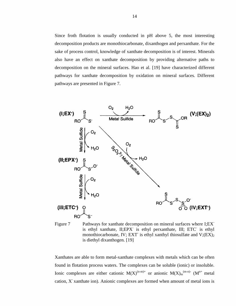
Since froth flotation is usually conducted in pH above 5, the most interesting

decomposition products are monothiocarbonate, dixanthogen and perxanthate. For the

sake of process control, knowledge of xanthate decomposition is of interest. Minerals

also have an effect on xanthate decomposition by providing alternative paths to

decomposition on the mineral surfaces. Hao et al. [19] have characterized different

pathways for xanthate decomposition by oxidation on mineral surfaces. Different

pathways are presented in Figure 7.

Figure 7 Pathways for xanthate decomposition on mineral surfaces where I;EX

-

is ethyl xanthate, II;EPX- is ethyl perxanthate, III; ETC

- is ethyl

monothiocarbonate, IV; EXT- is ethyl xanthyl thiosulfate and V;(EX)2

is diethyl dixanthogen. [19]

Xanthates are able to form metal-xanthate complexes with metals which can be often

found in flotation process waters. The complexes can be soluble (ionic) or insoluble.

Ionic complexes are either cationic M(X)(n-m)+

or anionic M(X)m(m-n)-

(Mn+

metal

cation, X- xanthate ion). Anionic complexes are formed when amount of metal ions is

15

lower than xanthate ions and cationic complexes are formed when the amount of

metal ions is higher than xanthate ions. Insoluble metal xanthates are formed when

xanthate and metal ions react in stoichiometric concentrations. Xanthates are able to

form 1:1 complexes with Pb2+

, Cd2+

, Zn2+

, Ni2+

, Co2+

and Cu2+

. Other metal-xanthate

complexes may also occur. Xanthate metal complexes have quite low solubilities e.g.

Zn(EtX)2 has a solubitity of 9.0*10-4

mol/L in 20°C water. [15]

4 Capillary electrophoresis

Electrophoresis is the movement of ions in an electric field. This often performed by

applying a current across a narrow-bore open capillary where the separation of

substances takes place. Other electrophoresis techniques include methods such as slab

gel electrophoresis, but it has lower separation efficiency and longer analysis time.

High separation efficiency of capillary electrophoresis (CE) is based on large surface

area to volume ratio and the minimizing of peak widening due to thermal reasons.

The advantages and disadvantages of capillary electrophoresis are presented in Table

V. [20-25]

Table V Advantages and disadvantages of capillary electrophoresis [20-23, 25]

Advantages Disadvantages

High efficiency Method reproducibility

Short analysis time Sensitivity

Small samples needed (1-50nl) Injection accuracy

Produces small amount of analysis waist

Wide range of applications

Operates in aqueous media

Method development is relatively simple

Automated instrumentation

16

The capillary is fused silica with bore diameter varying between 20-200 µm. The

length of the capillary varies often between 20-100 cm.. Capillaries can be made from

glass or Teflon but silica usually preferred since it has certain advantages over glass

and Teflon e.g. it won’t break so easily as glass. High voltage (10-30 kV) is applied

across the capillary ends which generates electro-osmotic (EOF) and electrophoretic

flows that transport substances in different velocities according to their charge

density. Thus the substances arrive in different order to the detector where migration

time and absorbance level can are measured. [20-23]

The detector is usually based on absorbance of ultraviolet (UV) -light, but other

detectors are also sometimes used. These include detectors such as laser-induced

fluorescence, conductivity, electrochemical, mass spectrophotometry, radioactivity

and refractive index detectors. The absorbance of UV light is done through a capillary

window, where the polymer coating over the capillary has been removed. Substances

which don’t absorb UV-light can also be detected with a UV absorbance detector by

using a buffer which absorbs light strongly. When the substance zone arrives to the

detector it is recognized by its ability to not absorb light. In other words the

absorbance level decreases below the zero level. This occurs every time when zones

of substances that don’t absorb UV-light arrive to the detector. [23, 26, 26]

Capillary electrophoresis instrumentation setup consists of inlet and outlet buffer

electrolyte reservoirs, sample reservoir, high voltage power supply, capillary, detector

and a computer control. The capillary is coated with a polymer to protect it. The

polymer is removed where the detector is since the detection is made through the

capillary usually with a UV-detector. CE instrumentation setup is presented in Figure

8.

17

Outlet reservoir

SampleInlet

reservoir

Computer control

Detector

HV Power supply Electrode

Capillary

Figure 8 CE instrumentation setup [21]

4.1 Electrophoresis and electro-osmosis

The capillary is filled with a background electrolyte (buffer). Sample is introduced to

the capillary by inserting the capillary inlet end from the buffer vial to the sample

vial. Sample is injected by using different methods to the capillary. The inlet end of

the capillary is inserted back to the buffer vial after which voltage is turned on

between the capillary ends. The outlet of the capillary is usually in the same vial as

the negative electrode. This is called normal polarity. When the outlet is in the same

vial as the positive electrode the setup is called reversed polarity. Positively charged

ions are attracted to the negative electrode and start to move towards it. Negative ions

are attracted to the positive electrode. This movement caused by electrical voltage is

called electrophoretic flow (EPF). When the pH of the buffer is above 2 the silica

capillary becomes ionized and is negatively charged. Thus the positively charged ions

accumulate as a layer on top of the silica surface forming an electrical double layer

(Stern layer). A diffusion layer, forming of mainly positively charged ions, is

stratified loosely on top of the Stern layer. When a voltage is applied to the capillary

negatively charged ions pull the loose positively charged ions with them. This

movement is called electro-osmotic flow. If EOF is greater than the repulsion of

18

positively charged ions towards the positively charged electrode caused by

electrophoretic force, the positively charged ions will also move forward towards the

detector. [20-23] The mobility of analytes has been expressed in formula 3. [27]

(3)

Where µa apparent mobility

µEP electrophoretic mobility

µEO electro-osmotic mobility

With cations µEP and µEO are parallel and with anions vice versa if the system has been

setup as normal polarity. Anions will go through the capillary only if µEO is larger

than µEP. Apparent mobility is calculated with formula 4.

(4)

Where Ld capillary length to detector

Lt capillary total length

t migration time

U applied voltage between capillary ends

Electro-osmotic mobility can also be calculated with the previous by replacing

migration time with EOF peak time.

19

4.2 Sample injection

Samples are introduces to the capillary by replacing the capillary inlet vial from the

buffer vial to the sample vial. The length of sample zone injected should be less than

1-2 % of the total length of the capillary. Hydrodynamic sample injection is the most

preferred injection method available. Sample is introduced to the capillary by the

means of either pressure from the inlet, by vacuum from the outlet or by siphoning.

Hydrodynamic injection is almost independent from the sample matrix. That is why it

is often preferred over others injection methods. [20-22]

Electrokinetic sample injection, which is often called field amplified sample injection

(FASI), is another method for sample injection. Capillary inlet is placed in to the

sample vial and voltage is applied between the capillary ends. Analytes move to the

capillary due to electrophoretic flow. EOF can help to inject the analytes to the

capillary if EOF moves towards the outlet. If EOF moves to the opposite direction, it

will hinder the injection. Molecules with high electrophoretic mobilities will migrate

to the capillary more rapidly. That is why FASI will not give a uniform injection.

Field strengths are often 3-5 times lower than the field strengths used in separation.

Injection times are usually 10-30 s. Pressure and voltage are many times used in

combination to inject the sample to the capillary. In this case the injection method is

called pressure assisted field amplified sample injection (PA-FASI). This

combination can be used if EOF migrates the analytes away from the capillary to

overcome this problem. PA-FASI has the same problem as FASI as the molecules

with higher electrophoretic mobilities will migrate more rapidly, the injection will not

be uniform. [20-23, 28]

Stacking is a method where sample that has a much lower conductivity than the

buffer electrolyte is injected to the capillary hydrodynamically. Ions of the sample are

stacked (compressed) into zones in the sample region near the buffer region. Opposite

polarity is turned on to push the end of the sample matrix out of the capillary while

the stacked ions of the sample stay near to the buffer region. After this the inlet end of

20

the capillary is set in the buffer vial and normal separation voltage is applied.

Stacking requires filling the capillary up to two thirds of the total capillary length. [5,

20, 21, 29, 30]

4.3 Modes of operation

Capillary electrophoresis has a group of operation modes which have divergent

operative and separative characteristics. The modes are capillary zone electrophoresis

(CZE), capillary isoelectric focusing (CIEF), capillary gel electrophoresis (CGE),

capillary isotachophoresis (CITP), micellar electro kinetic capillary chromatography

(MEKC) and capillary electro chromatography (CEC). Since the focus of this

research was on CZE, it and only two of the previously mentioned modes are shortly

described below to give some kind of a view of these modes and how the differ from

one another. [20, 22]

Capillary zone electrophoresis is the simplest form of CE and it is also the mode

which was used in the experimental part of this research. The capillary is filled with a

homogenous buffer solution after which sample is injected to it. Constant field

strength is applied throughout the length of the capillary which causes analytes to

migrate in to different zones due to EOF and EPF. [20, 22]

Molecules will stop migrating if they become neutral in an electric field. Capillary

isoelectric focusing is performed in a pH gradient. The pH is high at the cathode and

low at the anode end. Carrier ampholytes applied in a series generate the pH gradient.

Ampholytes migrate in the capillary, when voltage is applied, according to their

charge towards different electrodes. When ampholytes reach their isoelectric point

they will stop migrating, since they will become neutral. Thus the molecules will be

in different zones. [20, 22, 31]

Capillary isotachophoresis is carried out by filling the capillary with a leading buffer

solution which has higher mobility that any of the analytes. Sample is the injected to

21

the capillary after which a terminating buffer is introduced to the end of the capillary.

The terminating buffer has a lower mobility than any of the analytes. Thus the

analytes will separate between the leading and terminating buffer. [20, 22, 32] An

illustration of how analytes separate in different zones when using CZE, CIEF and

CITP is expressed in Figure 9.

a dc b a

T L

LT

ab

e fg h

d bc d

rfgc

def g

a aa a

bb

bb

cc

cc

dd

dd

ee

e

e

fff

f

gg

gg

hh

hh

t=0

t=0

t=0

t>0

t>0

t>0

CZE

IEF

ITP

Figure 9 Illustration of CZE, CIEF and CITP zonal separation [20]

5 On-line measuring

On-line monitoring of environmental or process samples can help control and

understand processes better. The word “on-line” in this context means that sampling

and analysis is automated while sample transport is integrated. If compared to e.g.

off-line monitoring, sampling is manual, analysis is manual or automated and sample

transport is done in a remote or centralized laboratory. Different classes of process

analyzers are presented in Table VI. [33]

22

Table VI Classes of process analyzers [33]

Process analyzer Sampling Sample transport Analysis

Off-line manual to remote or centralized laboratory

automated/manual

At-line discontinuous/manual to logical analytical

equipment automated/manual

quick check

On-line automated Integrated automated

In-line integrated no transport automated

Noninvasive no contact no transport automated

Physical parameters, such as temperature, pressure and density, may have an effect on

chemical reactions. These are often more easily measured on-line, than chemical

parameters, but they do not explain the overall process. An on-line chemical

measurement method is needed to determine variables that physical parameter

measurements cannot explain such as chemical composition. This requires a fast and

reliable analysis method to able to intervene the process according to the situation.

On-line measurements can aid in the following issues: [33]

Making the process more efficient

Ensure and enhance product quality and uniformity

Comprehension of the process

Increasing safety by monitoring process and reactor conditions

Saving raw materials, labor costs, process waste and etc.

Saving time for analysis and sample transport

On-line monitoring of chemical reactions includes methods which are based on

techniques such as ultrasound, dielectric spectroscopy, optical spectroscopy, particle

size analysis, chromatography, electroanalytical methods, mass spectrometry,

rheometry, NMR spectroscopy and etc. [33] An on-line Capillary electrophoresis

system has been used previously to e.g. monitor the production of carboxylic acid by

yeast in bioreactor cultivations [34] and to monitor water-soluble ions in pulp and

paper machine waters [35].

23

H. Turkia et al. [34] developed a method where a sample was pumped from a

bioreactor, through a filter, to a CE flow-through sample vial. CE measured the

production of carboxylic acid by two yeast, K. lactis and S. serevisiae. The sampling

interval was either once per hour or once per every two hours and system was able to

run automatically and continuously up to six days. The system setup of the on-line

CE monitoring method which H. Turkia et al. used is presented in Figure 10.

Figure 10 Schematic of the on-line monitoring system used to produce

carboxylic acid [34]

R. Kokkonen et al. [35] used an on-line CE system to monitor water-soluble ions in

pulp and paper machine waters. Requirements for water circulation have increased

which means the concentrations of water-soluble compounds will increase also. It is

highly likely that this will lead to chemical precipitation and equipment corrosion. A

batch-type feeding unit was used in the CE unit to refill the samples. The system was

suitable for the task and it could run continuously up to one week.

S.Luukkanen et al. [36] developed a method for measuring xanthate concentrations

from flotation tailings with an on-line potentiometric titration system (Murtac OMT

20 DX). They conducted a two-week measuring experiment in in Pyhäsalmi Finland

concentrating plant. The tailings slurry was directed through several clarifying stages

before filtering it by using a CERAMEC filter. The clarifying stages were used since

the pulp density in the tailings was high and because of this the filter would have

been blocked rapidly. Thus the sample would not have been able to be transported to

24

the analyzer. The xanthate amounts in the flotation tailings varied between 3-11 ppm

during a two-week measuring period.

A method, which used similar titrator as S. Luukkanen et al. used, was previously

operated in Siilijärvi Finland concentration plant to measure seasonal fluctuations of

species which dissolved from minerals and air (Ca2+

, CO32-

and HCO3-) to a flotation

pond by P. Stén et al. [37] A sintered alumina CERAMEC filter proved to be a

sufficient way to clear the sample from the pond.

Xanthates have also been analyzed, in a laboratory scale, by using an on-line UV-

spectrometer system. F. Hao et al. [38] used a method where they pumped solution

from a flotation cell through a micro filter with a peristaltic pump to a UV-

spectrometer. The UV-spectrometer was able to measure the sum of xanthates used

since no separation was done. The system could be used successfully for 50 minutes

at a time without blocking the filter.

In this research an on-line monitoring CE system was developed to measure collector

chemicals from flotation tailings. An automatic sampling unit and a CE method were

developed for this purpose. Normally the dosage of the collector depends on the feed

rate of the flotation circuit and the head grade of the valuable metal, but these

variables do not reveal the changes taking place in mineral composition of the ore.

Therefore it is worth monitoring the residual collector concentration in the flotation

tailings since excess usage of collector causes unnecessary costs and may even

disturb the process. The method development is presented in the experimental part of

the thesis.

25

Experimental part

6 Instrumentation and reagents

The aim of the experimental part of the thesis was to develop an on-line CE method

that is able to measure the concentration of collector chemicals from nickel flotation

tailings. Water used in these experiments was purified by Elga Centra R 60/120 water

purification system. This water is referred as pure water. Process water was received

from FQM Kevitsa Mining Oy in Finland as well as the tailings slurry from nickel

flotation with ca. 25 % solids. The ionic strength of samples affects the CE analyses.

Since collector concentrations were designed to be measured from nickel tailings, the

tailings were used as sample matrix when calibration standards were created. Hence

the ionic strength is closely the same.

Beckman Coulter P/ACE MDQ, with UV/vis diode array detection, capillary

electrophoresis was used to analyze all samples. The diameter of the capillary was 49

µm. The total length of capillary was 60 cm and the length to the detector was 50 cm.

The capillary was manufactured by Polymicro technologies and it was fused silica

coated with a polymer. The polymer was burned off at the detection window. A

peristaltic pump manufactured by Ismatec model BVB Standard with a multi-channel

pump head Ismatec CA-12, was used during on-line experiments to transport samples

to a flow-through vial inside the capillary electrophoresis. The pump was controlled

with a relay through the CE program. Two vial trays which had two large buffer

reservoirs (2 x 30 ml) were used since during long runs the buffer started to deplete.

Also the operator would not have to fill several small vials instead of a few large

ones. A vial tray which has two large buffer reservoirs is presented in Figure 11.

26

Figure 11 A vial tray with two large buffer reservoirs

A 10 µm Metrohm stainless steel rod filter, in conjunction with a settling tank, was

used to filter the samples for the capillary electrophoresis. Sampling was done with

an automated system which was specifically built for this study. The system is

presented in method development section.

Preliminary experiments were made in Lappeenranta University of Technology

before the concentrator measurement campaign. Sodium isopropyl xanthate (SIPX)

and sodium di(isobutyl) dithiophosphinate (Aerophine) were measured during these

test. Sodium ethyl xanthate (SEX) was included to the experiments during the

concentrator measurement campaign. The purities and the providers of the reagents

are shown in Table VII.

Table VII Reagents used in the experiments

Chemical Abbreviation Purity Provider

Sodium isopropyl xanthate SIPX 87-89 % Flomin Inc.

Sodium di(isobutyl) dithiophosphinate

Aerophine 3418A 50-52 % (aq) Cytec

Industries Inc.

Sodium ethyl xanthate SEX 90 % Flomin Inc.

The background electrolyte solution (buffer) used was the same that Tuomas

Sihvonen [5] and Jussi Kemppinen [6] had used in their theses. The buffer was a 60

mM CAPS (3-(cyclohexylamino)propane-1-sulfonic acid) and 40 mM NaOH

27

solution. The solution was prepared by dissolving and mixing the substances to pure

water in an ultrasonic bath. The electrolyte solution seemed to keep relatively stable

for a long period of time. During the preliminary tests it was stored in a fridge and

before experiments the solution was allowed to warm to room temperature and it was

mixed in an ultrasonic bath. When the experiments were made during the

concentrator measurement campaign there was no ultrasonic bath available to mix the

solution. Instead, it was mixed manually, by shaking it in a bottle.

7. Preliminary experiments and method optimization

The validation process utilized in the experimental part is expressed in Figure 12.

Specificity and selectivity research

CE and sampling method optimization

(experimental design)

Repeatability(one concentration)

Robustness

Sensitivity, LOD, LOQ, Working range, linearity

(wide calibration concentration

range)

Process implementation (concentrator experiments)

Validation

Figure 12 A schematic of the utilized validation process

28

The method development was mainly made on the basis of preliminary experiments.

Before a two-week concentrator plant measurement campaign, experiments were

made in Lappeenranta University of Technology in Finland. Beckman Coulter

P/ACE MDQ capillary electrophoresis analyzer was used during the preliminary

tests. However, the CE broke before the concentrator measurement campaign and a

similar replacement instrument had to be used during the two-week measurement

campaign. A few experiments were made, with the replacement device, before the

campaign to see if the device would give similar results as previously and thus if it

could be used. The surface area of electro-osmotic flow peak was much lower on the

replacement CE and the peak did not stand out from the base line as clearly as with

the first CE used. This likely refers that less sample was injected to the capillary.

However it is likely that the surface areas are not compatible across devices. None the

less, collector chemicals could be qualified and quantified with the replacement

device with adequate precision.

Validation factors and components that affect them:

Specificity and selectivity

o Sample matrix

o Background electrolyte solution (buffer)

o Method parameters

o Chemical characteristics

Repeatability

o Stability of chemicals used

o Storage conditions

o Ambient conditions

LOD & LOQ

o Separation efficiency

o Baseline noise

o Peak identification and integration

o Chemical characteristics

o Detection method

29

Sensitivity, working range and linearity

o Calibration concentration range

o Calibration correlation

7.1. Method optimization: operating parameters

The first experiments were done off-line before switching to on-line. Experiments

started with the same method as T. Sihvonen et al. [39] had used in their tests. During

the injection negative voltage was applied to concentrate anions and external pressure

was added to exceed EOF. Process water and the filtrated tailings of nickel

circulation were tested with a capillary that had an effective range (length from inlet

to detection window) of 50 cm. The tailings sample was filtered with a 0.45 µm

syringe filter since otherwise the solid particles might have blocked the capillary.

The capillary was introduced by washing it first by pressure with NaOH for 10 min,

pure water 10 min and finally with the CAPS-buffer for 10 min. After this the actual

method was started. The method included three steps: buffer washing 3 min, injection

1 min and separation 10-20 min. Several runs were made with this method, which is

why there had to be a buffer wash between runs. The washing pressure was 40 psi.

The injection was done with a pressure assisted field amplified sample injection (PA-

FASI) method. The injection pressure was 1.5 psi and the voltage was 15 kV. The

polarity was on reverse. Once the separation started, the polarity was switched to

normal and the separation voltage was set to 20 kV. This method was tried on the

process water and filtered nickel flotation tailings. Process water did not show traces

of SIPX or Aerophine since the base line of CE graph was almost completely flat (i.e.

no spikes were shown). SIPX was found on the nickel flotation tailings, but no

Aerophine was detected. The peaks were identified by spiking i.e. adding reagents to

the sample matrix and seeing which peak grows. The method parameters, from where

the development was started, are presented in Table VII. CE graphs of process water

and nickel flotation tailings are presented in Figures 13 and 14.

30

Table VII Instrument parameters

Relay 2 on (pump) Time from start 2.9 min

Buffer wash Time 3 min

Pressure 40 psi

Injection

Voltage 15 kV

Pressure 1.5 psi

Time 1 min

Polarity reverse

Separation

Voltage 20 kV

Time 10-20 min

Temperature 20 °C

Polarity normal

Detection Wavelength 214, 225 and 301 nm

Figure 13 Process water CE graph. Applied wavelengths were 301 nm (blue/top

line), 225 nm (black/mid line) and 214 nm (red/bottom line). EOF-

peak can be seen approximately at time 5.5 min. Injection was done

with pressure and voltage. Separation voltage was 20 kV.

31

Figure 14 Filtered nickel circulation tailings CE graph. Applied wavelengths

were 301 nm (blue/top line), 225 nm (black/mid line) and 214 nm

(red/bottom line). EOF-peak can be seen approximately at time 5.5

min. SIPX can be seen clearly from the blue/top line approximately

slightly after 15 min mark. Injection was done with pressure and

voltage. Separation voltage was 20 kV.

SIPX and Aerophine peaks could be clearly seen from the sample matrix, when they

were added into it, even with relatively low concentrations. This indicated that the

injection seemed to be working. The peaks could also be seen during on-line tests.

Higher separation voltages were tried to make the method faster. The maximum

allowed separation voltage which could be set on the device was 30 kV. With this

voltage peaks still clearly separated from each other and the separation was made

faster. SIPX peak came approximately five minutes faster, during on-line tests, on 30

kV separation voltage when compared with 20 kV separation voltage. Because of this

it was decided to use the 30 kV voltage. Using higher separation voltages also makes

CE spikes higher and narrower which facilitates analyzing.

During on-line tests, a peristaltic pump was used to transport samples to a flow-

through sample vial. Sample was circulated from a beaker glass to the vial and back.

The circulation was first set to be on the whole method. The pump speed was set to

be relatively low since otherwise it would spit some of the samples out from the flow-

32

through vial inside the CE and could cause problems with electricity. Capillary

electrophoresis gave several errors due to pressure and voltage leakage during

injection. Since the injection was done with a pressure assisted field amplified sample

injection method, it was deduced that pressure and voltage might leak because of the

flow through vial. Injection was set to be done with vacuum and voltage, instead of

pressure and voltage. By using vacuum, pressure could not leak since the inlet end of

the capillary was under the sample surface in the flow-through vial. Sample

circulation was set to be on only during the buffer wash which stopped voltage from

leaking.

Two vial trays with two large 30 ml buffer reservoirs (Figure 11) were acquired, since

during long runs the buffer started to deplete. The manufacturer announced in the

user manual that the reservoirs could hold up to 30 ml of solution. However, when

experiments were made by adding 30 ml of buffer to the reservoirs, they slightly

flood over. If the reservoirs were filled too full, some electrical discharges could be

seen during usage and the experiment had to be immediately stopped. It was noted

that when 15 ml of buffer was added in a reservoir, no electrical discharges could be

seen. Since the reservoirs were relatively large, some power was sure to be leaked

and the device informed about it. An “external adapter” option had to be selected

from the device program to bypass this problem.

Repetition experiments were made with nickel circulation tailings where SIPX and

Aerophine were added to see how the depletion of buffer affects the analysis. This

was done with the special vial trays, where the buffer reservoirs were filled with 15

ml of buffer. It was noted that after 30 runs, each having a 20 min separation phase,

the area of SIPX peak was approximately 80 % of the first run.

The nickel circulation tailings had to be filtered since otherwise the solids would have

blocked the 50 µm diameter capillary. The slurry contained 25 % of solids and the

experiments made used mainly tailings which were filtered with a 0.45 µm syringe

filter. No solids could be seen in the filtered matrix. Samples which were filtered with

the 10 µm rod filter contained some solids. The filter was able to remove

approximately 99 % of solids and the matrix was slightly dark. The slurry, filtered

33

with the 10 µm rod filter, was analyzed with CE to see if the non-filtered solids

would interfere the analysis. A few small sharp peaks could be seen in the CE graph

on all applied wavelengths, which implies that solid particles pass the detector. This

did not seem to disturb the analysis, even when several repetitions were made.

As an outline optimization to operating parameters was done to the following issues:

Separation voltage

Flow-through vial pump speed

Injection pressure

o Pressure was reversed to vacuum

CE program configuration

o “External adapter” option was selected to bypass current leakage

Amount of runs that can be done before the buffer depletes

7.2 Method optimization: sampling procedure

Approximately 40 liters of nickel circulation tailings slurry was obtained for

preliminary experiments. During the transportation and storing most of the solids had

settled to the bottom of the storage barrel and the surface of the slurry was clear. The

settled solids had a clay-like feeling when trying the bottom with a stick. The slurry

was mixed with a 3-blade propeller. Since the concentration of solids was high, 25 %

in mass, the slurry had to be left to mix overnight so that it would be homogenous

once filtrated.

A peristaltic pump, with a capacity of 320 ml/min (theoretical value, real value with

water 250 ml/min), and a 20 µm stainless steel rod filter were used in filtration tests.

The filter was attached to the other end of a 3 m tube, with a 4 mm diameter, and the

pump was installed to the other. However, once the filter was sunk under the mixed

slurry and the pump was turned on, the speed of the filtration was so low that it was

decided to get a pump with a larger 1.2 l/min capacity. Also the 20 µm rod filter

34

seemed to let through a relatively large amount of solids which could be seen with the

human eye. The filtrate was relatively dark in the beginning of the filtration, before a

cake was formed on top of the filter and started to do most of the filtration. Therefore

a filter with a smaller 10 µm mesh size was tested. The higher 1.2 l/min capacity was

theoretically possible with no counter pressure. However, it was able to pump water,

with a 3 m hose attached and no filter, approximately only 330 ml/min. When the

mixed tailings slurry was filtered with the higher capacity pump and a smaller mesh

size rod filter the speed of the filtration was approximately 19 ml/min. The filtrate

was quite clear since the filter removed approximately 99 % of solids. The filtrate

became even clearer during the filtration since a cake was formed on top of the filter

and started to do most of the filtration. The hose and filter were backwashed with

water for 10 s time and with air for 5 s time to remove the formed cake on top from

the filter and to clear the hose from filtrate and washing water. This was done since

after a few minutes of filtration, the cake became so thick that it restricted too much

of the flow and it was not reasonable to continue the filtration with such a slow speed.

The filtration volume in relation to filtration time is illustrated in Figure 15.

Figure 15 Filtration volume expressed as a relation to filtration time. The graph

starts at 130 s time since it took that much time to fill the 3 m hose

between the filter and the pump. The filtration speed calculated from

the slope is approximately 19 ml/min.

y = 0.3143x - 39.429 R² = 0.9723

0

10

20

30

40

50

60

0 50 100 150 200 250 300

Vo

lum

e a

fte

r p

um

p, m

l

Time, s

35

Next, a 10 minute settling was tried prior filtration to see if it would speed up the

filtering. It was concluded that a single-stage sample preparation by filtration would

be too slow. For this reason an estimate for settling speed had to be determined. A

measuring cylinder was filled with the mixed slurry and the time which the solids

settled was measured. In the beginning the settling speed was slightly above 0.2

cm/min but after 162 min of settling it had dropped down to 0.13 cm/min. The solids

settled relatively slowly, but there was a clear cut between the two phases. The

settling in a measuring cylinder is shown in Figure 16.

Figure 16 Settling of the nickel circulation tailings. Settling times from left to

right: 12, 67 and 137 min.

Sampling was planned to be done from Multiplexer, used as a sampler for the Courier

analyzer, manufactured by Outotec, in a real flotation process at FQM Kevitsa

Mining Oy. Courier is an on-line analyzer that measures element grades from process

streams. The results from Courier can be used to control the process. It uses

wavelength dispersive x-ray fluorescence (WDXRF) as a measuring technique and

can give for example the copper grade (%) in a process sample. Process samples are

fed to Courier from sample Multiplexer (MXA), which selects one sample at a time

to be analyzed. The sample, for measuring collector chemicals, was taken

36

automatically from Courier feed box at the MXA, when the tailings from nickel

flotation was fed to the box. The flow chart is presented in Figure 17 after which the

process is described.

37

Fig

ure

17

S

yst

em f

low

ch

art

38

Slurry is pumped via pump P1, which is a diaphragm pump, to a settling tank for 48

seconds. The slurry is left to settle for 24 minutes. After settling it is pumped, via 10

µm rod filter, with a peristaltic pump P2 to a sample tub inside the sample basin for 3

minutes. Following the filtration, valves V3 and V2 open automatically and back-

wash the pipelines, filter and bottom of the settling tank, are backwashed for 18

seconds after which the valves close. The water used for washing is the

concentrator’s raw water. Next the pipelines and filter are cleared with air and the

bottom of the settling unit opens clearing the tank of excess sample. Valves V1 and

V4 open automatically for 24 seconds. The automation is done by using time relays.

Valve V5 can be manually opened if the sample tank needs to be cleared. CE and the

multi-channel peristaltic pump P3 work independently regardless of the sample

preparation unit. CE sends a command to pump P3, once previous analysis is done, to

start pump sample from the sample reservoir inside the sample tank to the flow-

through sample vial. Sample tub overflow is led out of the system from the bottom of

the sample basin. Settling basin and units prior that, were one floor up from the rest

of the system which were in the same booth as the Courier analyzer unit. A

Schematic diagram of the Courier installation layout is presented in Figure 18.

Figure 18 Courier installation layout

39

As an outline optimization to sampling procedure was done to the following issues:

Filter mesh size

o A smaller 10 µm mesh size rod filter was selected instead of a 20 µm

filter since it would not have filtered the solids as well.

The times of various stages

o Filtration time

o Counter-current water wash time

o Counter-current air blow time

o Settling time

o Slurry pump (P1) operating time

8 Process implementation

A two-week measurement campaign was carried out in the end of January 2014 at

FQM Kevitsa Mining Oy concentrator plant, in northern Finland. Kevitsa Mining Oy

employs more than 300 workers and the estimated operating time is 29 years. The

concentrator produces approximately 85 000 tons/year of nickel concentrate and

70 000 tons/year of copper concentrate. After the ore has gone through crushing and

grinding, copper is recovered in several stages of flotation. The tailings of copper

flotation are fed to nickel circuit and the tailings of nickel flotation are fed to pyrite

flotation. SIPX and SEX are added to the beginning of nickel flotation. Aerophine is

added to the beginning of copper circuit.

Sample pretreatment unit which was developed on the basis of preliminary

experiments was introduced during these measurements. Before the campaign, the CE

which was used in method development broke and experiments had to be done with a

similar replacement device. SIPX and Aerophine collectors were tested during the

preliminary tests. SEX was introduced in addition to these in the concentrator. There

40

was no previous experience on how SEX would behave during long period on-line

runs with CE. T. Sihvonen [5] had studied Potassium-ethyl-xanthate off-line with CE

in his studies.

Issues which needed to be taken in consideration while implementing the system are

listed below:

Sample pretreatment

o Sample should be relatively clear (as little of solids as possible)

o Sample is taken from the correct stream

Sample feed

o Enough sample is fed

Process conditions

o Humidity should not be too high.

o CE should be placed on a stable platform (no vibration).

o Temperature should be close to laboratory conditions.

8.1 Sample pretreatment

The automatic sampling system was introduced during the concentrator measurement

campaign. The system was automated by using time relays. One of the relays was

broken and thus the system skipped the last phase of the sampling loop. Because of

this, during the first week of measurements, the system had to be partly manually

operated. At the end of the first measurement week, a new relay arrived and after

switching it with the broken one, there were no problems due to the relay.

The system was set to take a sample from the courier feed box when the tailings of

nickel circulation arrived to it. However, the sample loop started quite often

immediately after the previous had ended, even if the Courier feed box held a wrong

sample. This was probably due to wrong parameters in Couriers program. New

parameters were obtained at the end of the measurement campaign, but there was no

41

time to test them in action. The new parameters are expected to be tested during a

second measurement which will be reported separately from this thesis.

Approximately 1/3 of experiments went wrong due to wrong sample intake. During

the campaign the system was set to do measurements over one night, which was the

longest single run. The wrong samples could be seen from CE graphs since the

graphs were much different from the nickel flotation tailings graphs.

Optimization of the sampling unit had to be mainly done in the amount of sample

taken from the Courier feed box and the level of the filter in the settling tank. The

amount of sample pumped to settling tank was relatively low. It was increased by

raising the operating pressure of the slurry pump and increasing the pumping time.

The amount of slurry pumped to the settling tank was also affected by the primary

sample flow from the process to Multiplexer. However it was not possible to alter the

amount of primary sample flow. The amount, and thus the level, of slurry pumped to

the settling tank varied slightly between measurements. Because of this the filter had

to put in a certain height, so that it would be under the slurry surface. If it would have

been put too low, it would have clogged since a large amount of the solids settle to

the bottom of the tank. A quite good height for the filter was found by trial and error.

8.2 On-line CE analyses

Capillary electrophoresis was used to qualify and quantify collector chemicals from

the tailings of nickel circuit. Four collectors were used at the concentrator, which

were SIPX, SEX, Aerophine and potassium-amyl-xanthate (PAX). PAX was not

studied in either during the preliminary experiments or at the concentrator. PAX is

used in sulfur flotation which is done after nickel flotation where the process sample

was taken. SIPX and Aerophine had been examined before the concentrator

measurement campaign. During the preliminary experiments SIPX was found from

the tailings of nickel circuit unlike Aerophine. Aerophine is added to the beginning of

copper flotation at low design rate and has thus quite possibly left the process before

the end of nickel circuit.

42

SEX was measured for the first time with the developed method during the campaign.

There was no previous experience how it would behave during long period on-line

experiments. Two large spikes were seen on xanthate detection wavelength 301 nm.

The peaks were distinguished by spiking, i.e. adding collector to the sample matrix

and seeing which peak grows. Identifying was slightly problematic since when

spiking was done with SIPX, both of the peaks grew. When spiking was done with

SEX only the latter peak grew. It is possible that SIPX pellets, used for preparing the

solution, contained also SEX as a production by-product of SIPX. SIPX came to the

detector before SEX. The amount, of which SEX peak area grew when SIPX pellets

were added, seemed to be rather constant in relation to the peak area which SIPX

grew. This relation was used as a correction factor when SEX calibration curve was

made, since the calibration curves of all three collectors were made in the same

matrix (SIPX influenced SEX peak area) and the issue was noticed only after the

calibration solutions had been made and analyzed. In addition, if the calibration

curves had been made individually for all three collectors, it would have taken a too

large portion of the time which was available at measurement campaign.

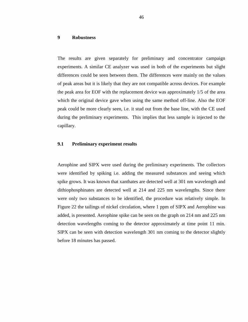
After identifying the spikes and creating a calibration curve for all three collectors,

the sampling unit and analyzer were tested in conjunction and the results were

compared with the dosage values of the collectors. Nickel flotation tailings, where 1

ppm of SIPX and SEX has been added, is presented In Figure 19. The analyzed

tailings, used in Figure 18, were divided into two portions. To one portion a small

amount of SEX was added. This is presented in Figure 20. SIPX was added to the

second portion, which is presented in Figure 21.

43

Figure 15 Nickel circulation tailings where 1 ppm of SIPX and SEX has been

added. Detection wavelength is 301 nm.

Figure 20 Nickel circulation tailings where a small amount of SEX has been

added in addition to the 1 ppm addition of SIPX and SEX. Detection

wavelength is 301 nm.

44

Figure 21 Nickel circulation tailings where a small amount of SIPX has been

added in addition to the 1 ppm addition of SIPX and SEX. Detection

wavelength is 301 nm.

It can be clearly seen that when SEX was added to the nickel circulation tailings in

Figure 20, which included 1 ppm of SIPX and SEX, only the latter of the two large

spikes grew. This obviously means that the latter spike represents SEX. But when

SIPX was added to the tailings, both of the spikes grew. However, the first of the two

large spikes grew more over the other.

The pressure used to wash the capillary during the preliminary experiments was set to

40 psi. However the replacement CE could not keep the pressure so high. The

program stopped some of the runs due to this. The washing pressure was lowered to

30 psi which stopped the program from giving errors. The reduction did not seem to

affect the analysis.

The sample tank had a small reservoir (a few tens of milliliters) inside of it where the

filtrate was pumped. The filtrate overflow ran to the sample tank. The overflow

filtrate was led out from the bottom of the tank. Since the volume of the reservoir was

small, the time which the multi-channel peristaltic pump P3 operated had to be

45

decreased to one minute. The reservoir was drained empty during the one minute

pumping but the pump did not unnecessarily operate as long as it did previously.

Since the outlet of the flow-through vial was higher than the inlet, and the capillary

and electrode sunk under the sample surface, it did not matter if the sample ran out

from the reservoir inside the sample tank. The final method which was improved on

the basis of preliminary experiments and concentrator measurements is presented in

Table VIII.

Table VIII Final CE method

Relay 2 on (pump) Time from start 1 min

Buffer wash Time 3 min

Pressure 30 psi

Injection

Voltage 15 kV

Pressure 1.5 psi

Time 1 min

Polarity reverse

Separation

Voltage 30 kV

Time 10-20 min

Temperature 20 °C

Polarity normal

Detection Wavelength 214, 225 and 301 nm

46

9 Robustness

The results are given separately for preliminary and concentrator campaign

experiments. A similar CE analyzer was used in both of the experiments but slight

differences could be seen between them. The differences were mainly on the values

of peak areas but it is likely that they are not compatible across devices. For example

the peak area for EOF with the replacement device was approximately 1/5 of the area

which the original device gave when using the same method off-line. Also the EOF

peak could be more clearly seen, i.e. it stud out from the base line, with the CE used

during the preliminary experiments. This implies that less sample is injected to the

capillary.

9.1 Preliminary experiment results

Aerophine and SIPX were used during the preliminary experiments. The collectors

were identified by spiking i.e. adding the measured substances and seeing which

spike grows. It was known that xanthates are detected well at 301 nm wavelength and

dithiophosphinates are detected well at 214 and 225 nm wavelengths. Since there

were only two substances to be identified, the procedure was relatively simple. In

Figure 22 the tailings of nickel circulation, where 1 ppm of SIPX and Aerophine was

added, is presented. Aerophine spike can be seen on the graph on 214 nm and 225 nm

detection wavelengths coming to the detector approximately at time point 11 min.

SIPX can be seen with detection wavelength 301 nm coming to the detector slightly

before 18 minutes has passed.

47

Figure 22 CE graph of nickel circulation tailings where 1 ppm of SIPX and

Aerophine have been added. Injection was done with pressure and

voltage. Separation voltage was set to 20 kV. Applied wavelengths

were 301 nm (blue/top line), 225 nm (black/mid line) and 214 nm

(red/bottom line).

During the first on-line experiments with CE, the instrument gave occasional errors

due to electricity and pressure leakage. The electricity leakage stopped when the

circulation in the flow-through vial was stopped during the injection. However this

did not solve the leakage problem with the pressure used during injection. Vacuum

was tried instead of pressure to exceed EOF. The injection done with vacuum and

voltage gave a surface area for EOF peak which was approximately 1,3 times larger

than the injection done with pressure and voltage. This implies that more analytes are

injected to the capillary. Even if circulation is not on during injection, pressure might

be pushed out slightly from the outlet of the flow-through vial.

Different separation voltages were tried mainly to test if the analysis could be made

faster but also to see if any problems would occur. This way the problems could be

avoided during the measurement campaign. Since SIPX came to the detector after

Aerophine, analysis time depended on it. When a 15 kV separation voltage was

applied, SIPX was not shown in the CE graph during a 20 minute separation phase.

48

However, when a 30 kV separation voltage was applied, SIPX was shown in the CE

graph slightly before 12 minutes of separation voltage had passed.

Repetition experiments were made with nickel circulation tailings where SIPX and

Aerophine were added to see how the depletion of buffer affects the analysis. This

was done with the special vial trays, where the buffer reservoirs were filled with 15

ml of buffer. It was noted that after 30 runs, each having a 20 min separation phase,

the area of SIPX peak was approximately 80 % of the first run. The depletion of the

buffer is expressed as relative reduction of SIPX peak area as a function of repetitions

in Figure 23.

Figure 23 The depletion of the buffer expressed as SIPX peak surface area

relative reduction as a function of repetitions

Since the 10 µm rod filter removed approximately 99 % of solids, the filtered tailings

from nickel circuit had to be tested in case the non-filtered particles would interfere

the analysis. A few small sharp peaks were shown on all applied detection

wavelengths due to solid particles which passed the detector. However these particles

did not seem to hinder the process even when several analysis repetitions of the

filtrate were made. CE graphs of nickel circulation tailings filtrate, where SIPX and

Aerophine have been added, are shown on in Figures 24 and 25 with two different

detection wavelengths.

y = -0.7341x + 101.2 R² = 0.9568

60

65

70

75

80

85

90

95

100

0 5 10 15 20 25 30 35 40

SIP

X p

eak

su

rfac

e a

rea,

%

Repetition number

49

Figure 24 CE graph of filtered tailings from nickel circuit with 5 repetitions. 1

ppm of SIPX and Aerophine were added to the filtrate. Applied

wavelength is 301 nm.

Figure 25 CE graph of filtered tailings from nickel circuit with 5 repetitions.

SIPX and Aerophine were added to the filtrate. Applied wavelength is

225 nm.

50

9.2 Concentrator experiment results

Calibration curves for SIPX, SEX and Aerophine were made on-line with the CE

method described in Table VIII. The standard solutions were made in the same matrix

(nickel circulation tailings) as the measurements were done. This way the ionic

strengths in the solutions should be close to same. Some variation might occur in the

ionic strength of nickel circulation tailings for example due to changes in ore

composition. Nonetheless this method should provide a good way to calculate

accurate concentrations for the collectors used. Calibrations standards were made in

the concentrations of 0.05; 0.1; 0.5; 1; 5; and 15 ppm. Since the tailings contained

SIPX and SEX in itself, the absorbance response of the blank solution was reduced

from the standard solutions. Also the constant was taken off from the calibration

curves. The electropherograms from CE calibration curve runs are shown in

APPENDIX I. The calibration curves for Aerophine, SIPX and SEX are presented in

figures 26, 27 and 28.

Figure 26 Aerophine calibration curve in nickel circulation tailings

y = 119971x R² = 0.9976

0

200000

400000

600000

800000

1000000

1200000

1400000

1600000

1800000

2000000

0 2 4 6 8 10 12 14 16

Pe

ak a

rea,

Au

*min

Concentration, ppm

Aerophine calibration curve

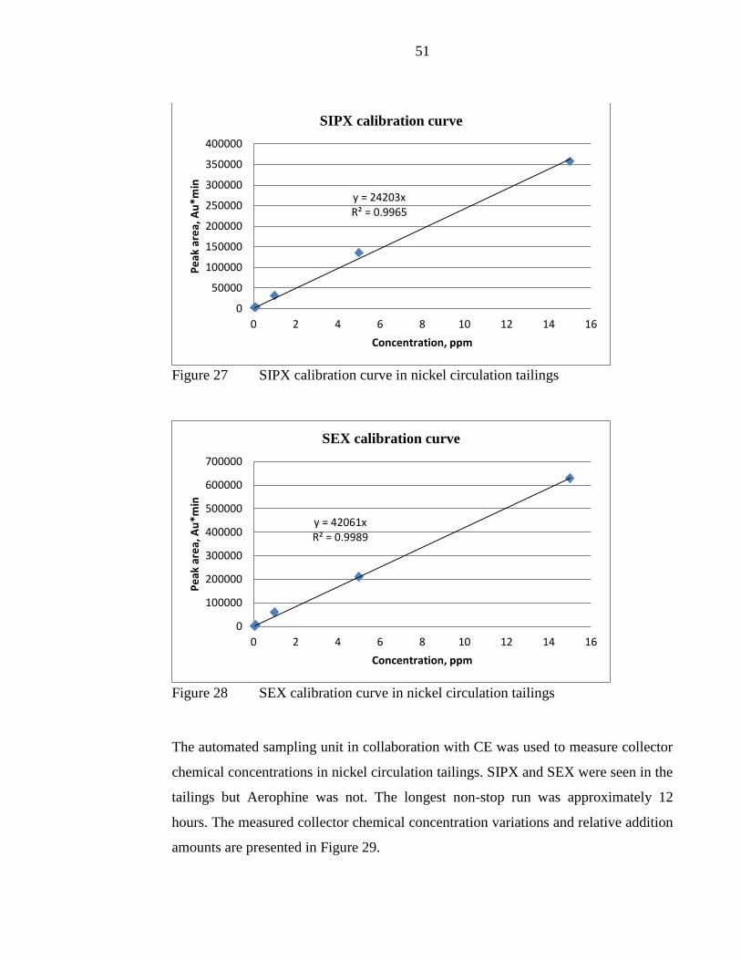
51

Figure 27 SIPX calibration curve in nickel circulation tailings

Figure 28 SEX calibration curve in nickel circulation tailings

The automated sampling unit in collaboration with CE was used to measure collector

chemical concentrations in nickel circulation tailings. SIPX and SEX were seen in the

tailings but Aerophine was not. The longest non-stop run was approximately 12

hours. The measured collector chemical concentration variations and relative addition

amounts are presented in Figure 29.

y = 24203x R² = 0.9965

0

50000

100000

150000

200000

250000

300000

350000

400000

0 2 4 6 8 10 12 14 16

Pe

ak a

rea,

Au

*min

Concentration, ppm

SIPX calibration curve

y = 42061x R² = 0.9989

0

100000

200000

300000

400000

500000

600000

700000

0 2 4 6 8 10 12 14 16

Pe

ak a

rea,

Au

*min

Concentration, ppm

SEX calibration curve

52

Fig

ure

29

M

easu

red c

once

ntr

atio

ns

and r

elat

ive

addit

ion a

mounts

of

coll

ecto

r

chem

ical

s in

the

pro

cess

53

The electropherograms from concentrator measurements are shown in APPENDIX II.

The values of migration time, peak area and concentration for each data point can

seen in APPENDIX III. Some correlation can be seen between the measured

concentrations and the relative addition amounts. During the longest single period 12-

hour run the concentrations seem to follow the addition amounts with a slight delay.

However if the individual runs are compared with each other’s, the correlation cannot

be seen. This might be explained for example due to buffer depletion or because the

capillary needs to be rinsed with NaOH so that no precipitate accumulation will

interfere the analysis. The capillary was rinsed in the beginning and end of each run

with 0.1 M NaOH.

It was noticed that SIPX pellets contained SEX as well. When SIPX was added to the

nickel circulation tailings the amount which SEX increased seemed to be rather

constant. The amount, which SEX grew, was approximately 12 % of the increase

amount of SIPX.

Limit of detection (LOD) and limit of quantification (LOQ) were calculated from

signal areas. Signal for analyte peaks were obtained from the lowest calibration

standards which had a signal to noise ratio larger than 10. The noise was obtained

from the baseline by integrating several noise peaks and calculating an average of

those. LOD was calculated as a signal area corresponding with the compound at the

lowest concentration to receive signal to noise ratio equal to 3. LOQ was calculated

the same way but with ratio 10. Electrophoretic mobilities for analytes were

calculated with equations 3 and 4 for calibrations standards between concentration

area of 0.05 ppm – 15 ppm. Relative standard deviation (RSD) for electrophoretic

mobility was determined to describe the spread of data with respect to the mean.

LOD, LOQ, µep and RSD of µep are presented in Table IX.

54

Table IX Validation measures LOD, LOQ, electrophoretic mobility and relative

standard deviation for electrophoretic mobility, for each collector

chemical

Collector chemical LOD, ppm LOQ, ppm µep, 10-8

m2v

-1s

-1 µep RSD, %

SIPX 0.0076 0.0254 -2.184 3.02

SEX 0.0029 0.0096 -2.392 6.36

Aerophine 0.0005 0.0018 -1.638 4.11

The migration time of SIPX and SEX changed between runs and during long runs.

Both collectors came to the detector faster over time as the run went forward. For

example during a 12-hour run, SEX came to detector approximately in 8 minutes at

the beginning. But after circa 12 hours had passed, SEX came to the detector more

than a minute earlier. This is probably due to ionic strength changes in the buffer

solution. Some shifting of the spikes, between different runs, could be seen during the

measurement campaign. This is probably caused by temperature and ionic strength

variations in the process. The used CE could control the temperature of the capillary

and sample storage but it is probable that, since the measurements were done on-line,

the samples did not have enough time to warm up to the set temperature. Migration

time shift of SIPX and SEX during approximately a 12-hour run is presented in

Figure 30 which can be used to estimate how the peaks will shift.

55

Fig

ure

30

S

IPX

and S

EX

mig

rati

on

tim

e sh

ift

duri

ng a

ppro

xim

atel

y 1

2 h

run

56

10 Conclusions

The aim of this thesis was the development of an on-line capillary electrophoresis

(CE) method for monitoring the behavior of collector chemicals in a flotation process.

For this reason a pretreatment filtration unit had to be designed to remove solid

particles, from nickel circulation tailings, which would otherwise interfere the CE

analyses. High concentrations of solids would likely block the capillary and/or cause

the CE graph to be un-interpretable due to additional spikes in the graph caused by

the solid particles. Also, a CE method needed to developed, because of this. Collector

chemicals had been examined previously by CE off-line. The method needed to be

enhanced to be able to work on-line in a real industrial process for long periods of

time. Method development was mainly done during preliminary experiments in

Lappeenranta University of Technology. Some minor tweaks were done to the

method when the system was tested in practice at a concentrator plant FQM Kevitsa

Mining Oy in northern Finland during a two week measurement campaign.

The designed pretreatment filtration unit removed approximately 99 % of the solids

in nickel circulation tailings. The remained particles did not hinder the analysis. The

used 10 µm rod filter, in conjunction with a settling unit, seemed to be a robust way

to filter the solid particles. In the beginning of the filtration more particles passed the

filter since a cake had not formed on top of the filter, which later started to do most of

the filtration. The system filtered a few deciliters of sample before the filter was

almost completely clogged. The sample amount was more than enough which was

needed for on-line CE analysis. The pretreatment filtration unit took samples

automatically approximately once every 30 minutes when nickel circulation tailings

came to the Courier multiplexer. However the system started to do another sampling

loop relatively frequently after the correct sampling loop had ended. Therefore the

system took a wrong sample to be analyzed. This effected approximately on one third

of the samples taken and the reason for wrong sample intake was probably involved

with the parameters set in the Courier program. The wrong samples could be clearly

spotted from the CE graphs since they differed from the correct ones so dramatically.

57

New Courier parameters will be tested in the future which will hopefully stop this

problem from occurring.

The developed CE method, described in Table VII, was able to detect sodium

isopropyl xanthate (SIPX) and sodium ethyl xanthate (SEX) from nickel circulation

tailings. Aerophine was not detected. This is likely due to the fact that Aerophine is

added to the beginning of copper circulation, which is set before nickel circulation,

and thus is removed before the end of nickel circulation. Limit of detection (LOD)

and limit of quantification (LOQ) for SIPX was 0.0076 ppm and 0.0254 ppm, for

SEX 0.0029 ppm and 0.0096 ppm and respectively for Aerophine 0.0005 ppm and

0.0018 ppm. The measured concentrations of SIPX and SEX were higher than LOD

and LOQ. The analysis of these components was possible to be done in less than 15

minutes which was less than sampling time.

When the calibration curve for SEX was created, the CE peaks widened on higher

concentrations and distinctly differed from the lower concentration peaks. High

concentrations lead to broad cross-sectional flow profiles and thus can be seen as

wide peaks. However when the wide peaks were integrated, the surface area values

did not seem to differ from the calibration line drawn with lower concentrations i.e.

the surface area values fitted to the line. This implies that the CE response taken from

higher concentrations could be used in the concentration determination.

The system can operate approximately one day on its own. After this the operator

mainly needs to change the buffer in the CE trays and check that the system is

working properly. The CE trays which had large buffer trays proved to ease the

workload of the operator since he did not have to fill several smaller vials instead of a

few larger ones. The system can be made to operate at a longer period if the analysis

interval is made longer. Collector chemical concentrations should not change in the

system relatively suddenly which should make the interval change possible. However

problems might still occur with the device itself since it is a relatively delicate

analyzer. Therefore it is better if the operator checks the system condition at least

once a day.

58

SIPX and SEX were added to the beginning of nickel flotation. During CE analyses,

it was noticed that the SIPX pellets contained also SEX, which is likely a production

by-product of SIPX. The amount, which SEX grew, was approximately 12 % of the

increase amount of SIPX. This could partially explain why the amount of SEX in

nickel circulation tailings was roughly 2-3 times the amount of SIPX. SIPX might

also react more actively with minerals which could be why there would be less of it in

the tailings of nickel circulation.

Slight correlation between the measured and addition amounts of collector chemicals

can be seen in Figure 29. During the longest single period 12-hour run, the

concentrations seemed to follow the addition amounts with a slight delay. However if

the individual runs are compared with each other’s, the correlation cannot be seen.

This might be explained e.g. due to buffer depletion or because the capillary needs to

be rinsed with NaOH so that no precipitate accumulation will interfere the analysis.

The capillary was rinsed in the beginning and end of each run with 0.1 M NaOH. The

correlation refers that the method seems to be working as intended. However more

data is needed on this issue in order to insure this fact. For this reason more

measurements will be made but they will be reported separately from this thesis.

In addition to the new Courier parameter tests and extra measurements, which should

be made to ensure that the system is working as intended, the next step could be

further automation in the CE program. In this research the CE spikes had to be

manually integrated with the program and the spike surface area had to be compared

to the calibration curve to get a concentration for each measurement and collector

chemical. This was relatively time consuming for the operator. The program should

be automated so that it would do this itself and send the data to the control room

programs which operators could use to control the process. Some shifting of the

spikes could be seen during the measurement campaign which might make automatic

spike integration difficult. A way to predict the shifting should be looked into more

closely. Also the on-line CE system could be altered so that it would measure the

concentrations of collector chemicals form other streams in addition to the nickel

59

circuit tailings. Robustness in process conditions should also be looked more closely

into.

Two electropherogram spikes came to the detector after SIPX and SEX nearly every

time (can be seen in APPENDIX II). These spikes can be seen with detection

wavelengths 214 and 225 nm. The spikes are likely degradation products of the

collectors. Jussi Kemppinen [6] had examined degradation products of collectors in

his Master’s thesis. The electropherograms spike which follows SEX spike is likely

ethyl thiocarbonate.

As a conclusion the developed on-line CE system proved to work in a real industrial

process relatively well. However some further testing in a concentrator plant and

development in CE program automation is needed so that the system would not be so

dependent on operator service.

60

References

1] R. D. Crozier, Flotation: Theory, Reagents and Ore Testing, Oxford, Great

Britain, 1992. ISBN: 0-08-041864-3

[2] Ullmann’s Encyclopedia of Industrial Chemistry, Vol B2: Unit Operations 1,

Gerhatz W., 5th

ed., VCH Verlagsgesellschaft, Federal Republic of Germany,

1988, Chapter 23

[3] S.K. Kawatra, Froth Flotation – Fundamental Principles, 2009

[4] M.J. Pearse, An overview of the use of chemical reagents in mineral

processing, Minerals Engineering, 18:139-149, 2005

[5] T. Sihvonen, Determination of collector chemicals from flotation process

waters using capillary electrophoresis, Master’s Thesis, Lappeenranta

University of Technology, Lappeenranta, Finland, 2012

[6] J. Kemppinen, Determination of decomposition products of flotation collector

chemicals using capillary electrophoresis, Master’s Thesis, Lappeenranta

University of Technology, Lappeenranta, Finland, 2013

[7] L.K. Wang, N.K. Shammas, W.A. Selke, D.B. Aulenbach, Handbook of

enviromentalengineering, Vol 12, Flotation technology, Humana press, New

York, 2010, ISBN 978-1-58829-494-4

[8] R.W. Rousseau, Handbook of Separation Process Technology, John Wiley &

Sons, USA, 1987, ISBN: 978-0-471-89558-9

[9] M.C. Fuerstenenau, G. Jameson, R. Yoon, Froth Flotation: A Century of

Innovation, SME, USA, 2007, ISBN-13: 978-0-87335-252-9

[10] S. Farrokhpay, The significance of froth stability in mineral flotation – A

review, Advances in Colloidal and Interface Science, 166:1-7, 2011

[11] Y. Hu, W. Sun, and D. Wang, Electrochemistry of Flotation of Sulphide

Minerals, Springer Berlin Heidelberg, 2009, ISBN 978-3-540-92178-3

61

[12] N.O. Lotter, D.J. Bradshaw, The formulation and use of mixed collectors in

sulphide flotation, Minerals engineering, 23:945-951, 2010

[13] A.N. Buckley, R. Woods, Chemisorption – the thrermodynamically favoured

process in the interaction of thiol collectors with sulphide minerals,

International Journal of Mineral Processing, 25:15-26, 1997

[14] S.M. Bulatovic, Handbook of Flotation Reagents: Chemistry, Theory and

Practice - Flotation of Sulfide Ores, Elsevier, Amsterdam, The Netherlands,

2007, ISBN: 978-0-444-53029-5

[15] J. Leja, Surface Chemistry of Froth Flotation, Plenum Press, New York, 1982,

ISBN: 0-306-40588-1

[16] B. McFadzean, D.G. Castelyn, C.T. O’Connor, The effect of mixed thiol

collectors on the flotation of galena, Minerals Engineering, 36-38: 211-218,

2011

[17] E. Bagci, Z. Ekmekci, D. Bradshaw, Adsorption behavior of xanthate and

dithiophosphinate from their mixtures on chalcopyrite, Minerals Engineering

20:1047-1053, 2007

[18] Z. Sun, W. Forsling, The degradation kinetics of ethyl-xanthate as a function

of pH in aqueous solution, Minerals Engineering, 10(4): 389-400, 1997

[19] F.P. Hao, E. Silvester, G.D. Senior, Spectoscopic characterization of ethyl

xanthate oxidation products and analysis by ion interaction chromatography,

Analytical chemistry, Vol. 72, No. 20: 4836-4845, 2000

[20] D.N. Heiger, High performance capillary electrophoresis – An introduction,

Hewlett-Packard Company, France, 1992

[21] H.H. Lauer, G.P. Rozing, High performance capillary electrophoresis, Agilent

Technologies, Germany, 2010

62

[22] Beckman Coulter, Introduction to capillary electrophoresis,

https://www.beckmancoulter.com/wsrportal/bibliography?docname=360643-

CEPrimer1.pdf, referred 3.12.2013

[23] T. Hiissa, H. Sirén, P. Savolahti, T. Kotiaho, Anionien ja kationien määritys

kapillaarielektroforeesilla – Menetelmän testaus ja optimointi, Posiva Oy,

Finland, 1999

[24] J. Cao, F.J. Hong, P. Cheng, Numerical study of radial temperature gradient

effect on separation efficiency in capillary electrophoresis, International

Communications in Heat and Mass Transfer, 34:1048-1055, 2007

[25] K.D. Altria, Enhanced pharmaceutical analysis by CE using dynamic surface

coating system, Journal of pharmaceutical and biomedical analysis, 31: 447-

453, 2003

[26] K.D. Altria, D. Elder, Overview of the Status and Applications of Capillary

Electrophoresis to the Analysis of Small Molecules, Journal of

Chromatography A, 1023:1-14, 2004

[27] M.L. Marina, A. Ríos, M. Valcárcel, Comprehensive analytical chemistry,

Volume XLV, Analysis and detection by capillary electrophoresis, Elsevier

B.V., Amsterdam, The Netherlands, 2005, ISBN: 0-444-51718-9

[28] F. Hissner, B. Daus, J. Mattusch, K. Heinig, Determination of flotation

reagents used in tin-mining by capillary electrophoresis, Journal of

chromatography A, 853:497-502, 1999

[29] Z. K. Shihabi, Stacking in Capillary Zone Electrophoresis, Journal of

Chromatography A, 902:107-117, 2000.

[30] J. P. Quirino and S. Terabe, Sample Stacking of Cationic and Anionic

Analytes in Capillary Electrophoresis, Journal of Chromatography A, 902:

119-135, 2000.

63

[31] L.H.H. Silverstand, J. Sastre Torano, W.P. van Bennekom, G.J. de

Jong,Recent development in capillary isoelectric focusing, Journal of

Chromatography A, 1204:157-170, 2008

[32] Z. Jarolímová, P. Lubal, V. Kanický, Analysis of renal stones by capillary

isotachophoresis, Talanta, 98:49-53, 2012

[33] Ullmann’s Encyclopedia of Industrial Chemistry, Vol 25, Wiley-VCH Verlag

GmbH & KGaA, Weinheim, 2012

[34] H. Turkia, S. Holmstöm, T. Paasikallio, H. Sirén, M. Penttilä, J.P. Pitkänen,

Online capillary electrophoresis for monitoring carboxylic acid production by

yest during bioreactor cultivations, Analytical chemistry, 85:9705-9712, 2013

[35] R. Kokkonen, H. Sirén, S. Kauliomäki, S. Rovio, K. Luomanperä, On-line

process monitoring of water-soluble ions in pulp and paper machine waters by

capillary electrophoresis, Journal of chromatography A, 1032: 243-252, 2004

[36] S. Luukkanen, P. Parviainen, M. Miettinen, P. Stén, S. Lähteenmäki,

A.Tuikka, Monitoring the composition of water of lotation slurries with an

on-line analyser, Minerals engineering, 16:1075-1079, 2009

[37] P. Stén, P. Parviainen, M. Miettinen, S. Luukkanen, V. Kaskiniemi, J.

Aaltonen, On-line analysis of flotation process waters at Siilijärvi (Finland)

apatite concentrating plant, Minerals engineering, 16:229-236, 2003

[38] F. Hao, K.J. Davey, W.J. Bruckard, J.T. Woodcock, Online analysis for

xanthate in laboratory flotation pulps with a UV monitor, International journal

of mineral processing, 89:71-75, 2008

[39] T. Sihvonen, A. Aaltonen, J. Leppinen, S. Hiltunen, H. Sirén, A novel

capillaty electrophoresis method with pressure assister field amplified sample

injection in determination of thiol collectors in flotation process waters,

Journal of chromatography A, 1325:234-240, 2014

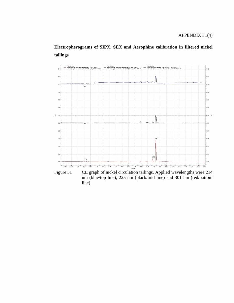
APPENDIX I 1(4)

Electropherograms of SIPX, SEX and Aerophine calibration in filtered nickel

tailings

Figure 31 CE graph of nickel circulation tailings. Applied wavelengths were 214

nm (blue/top line), 225 nm (black/mid line) and 301 nm (red/bottom

line).

APPENDIX I 2(4)

Figure 32 CE graph of nickel circulation tailings where 0,05 ppm of Aerophine,

SIPX and SEX were added. Applied wavelengths were 214 nm

(blue/top line), 225 nm (black/mid line) and 301 nm (red/bottom line).

Figure 33 CE graph of nickel circulation tailings where 0,1 ppm of Aerophine,

SIPX and SEX were added. Applied wavelengths were 214 nm

(blue/top line), 225 nm (black/mid line) and 301 nm (red/bottom line).

APPENDIX I 3(4)

Figure 34 CE graph of nickel circulation tailings where 1 ppm of Aerophine,

SIPX and SEX were added. Applied wavelengths were 214 nm

(blue/top line), 225 nm (black/mid line) and 301 nm (red/bottom line).

Figure 35 CE graph of nickel circulation tailings where 5 ppm of Aerophine,

SIPX and SEX were added. Applied wavelengths were 214 nm

(blue/top line), 225 nm (black/mid line) and 301 nm (red/bottom line).

APPENDIX I 4(4)

Figure 36 CE graph of nickel circulation tailings where 15 ppm of Aerophine,

SIPX and SEX were added. Applied wavelengths were 214 nm

(blue/top line), 225 nm (black/mid line) and 301 nm (red/bottom line).

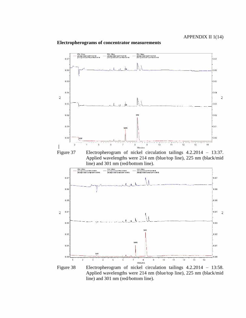
APPENDIX II 1(14)

Electropherograms of concentrator measurements

Figure 37 Electropherogram of nickel circulation tailings 4.2.2014 – 13:37.

Applied wavelengths were 214 nm (blue/top line), 225 nm (black/mid

line) and 301 nm (red/bottom line).

Figure 38 Electropherogram of nickel circulation tailings 4.2.2014 – 13:58.

Applied wavelengths were 214 nm (blue/top line), 225 nm (black/mid

line) and 301 nm (red/bottom line).

APPENDIX II 2(14)

Figure 39 Electropherogram of nickel circulation tailings 4.2.2014 – 14:20.

Applied wavelengths were 214 nm (blue/top line), 225 nm (black/mid

line) and 301 nm (red/bottom line).

Figure 40 Electropherogram of nickel circulation tailings 4.2.2014 – 14:41.

Applied wavelengths were 214 nm (blue/top line), 225 nm (black/mid

line) and 301 nm (red/bottom line).

APPENDIX II 3(14)

Figure 41 Electropherogram of nickel circulation tailings 5.2.2014 – 14:06.

Applied wavelengths were 214 nm (blue/top line), 225 nm (black/mid

line) and 301 nm (red/bottom line).

Figure 42 Electropherogram of nickel circulation tailings 5.2.2014 – 14:57.

Applied wavelengths were 214 nm (blue/top line), 225 nm (black/mid

line) and 301 nm (red/bottom line).

APPENDIX II 4(14)

Figure 43 Electropherogram of nickel circulation tailings 5.2.2014 – 15:23.

Applied wavelengths were 214 nm (blue/top line), 225 nm (black/mid

line) and 301 nm (red/bottom line).

Figure 44 Electropherogram of nickel circulation tailings 5.2.2014 – 15:49.

Applied wavelengths were 214 nm (blue/top line), 225 nm (black/mid

line) and 301 nm (red/bottom line).

APPENDIX II 5(14)

Figure 45 Electropherogram of nickel circulation tailings 5.2.2014 – 16:15.

Applied wavelengths were 214 nm (blue/top line), 225 nm (black/mid

line) and 301 nm (red/bottom line).

Figure 46 Electropherogram of nickel circulation tailings 5.2.2014 – 17:34.

Applied wavelengths were 214 nm (blue/top line), 225 nm (black/mid

line) and 301 nm (red/bottom line).

APPENDIX II 6(14)

Figure 47 Electropherogram of nickel circulation tailings 5.2.2014 – 18:00.

Applied wavelengths were 214 nm (blue/top line), 225 nm (black/mid

line) and 301 nm (red/bottom line).

Figure 48 Electropherogram of nickel circulation tailings 5.2.2014 – 18:26.

Applied wavelengths were 214 nm (blue/top line), 225 nm (black/mid

line) and 301 nm (red/bottom line).

APPENDIX II 7(14)

Figure 49 Electropherogram of nickel circulation tailings 5.2.2014 – 19:19.

Applied wavelengths were 214 nm (blue/top line), 225 nm (black/mid

line) and 301 nm (red/bottom line).

Figure 50 Electropherogram of nickel circulation tailings 5.2.2014 – 19:45.

Applied wavelengths were 214 nm (blue/top line), 225 nm (black/mid

line) and 301 nm (red/bottom line).

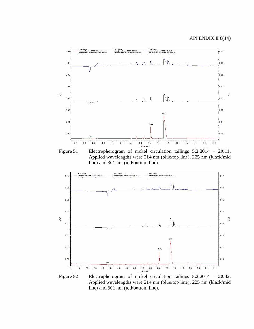
APPENDIX II 8(14)

Figure 51 Electropherogram of nickel circulation tailings 5.2.2014 – 20:11.

Applied wavelengths were 214 nm (blue/top line), 225 nm (black/mid

line) and 301 nm (red/bottom line).

Figure 52 Electropherogram of nickel circulation tailings 5.2.2014 – 20:42.

Applied wavelengths were 214 nm (blue/top line), 225 nm (black/mid

line) and 301 nm (red/bottom line).

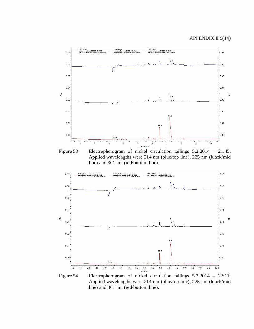
APPENDIX II 9(14)

Figure 53 Electropherogram of nickel circulation tailings 5.2.2014 – 21:45.

Applied wavelengths were 214 nm (blue/top line), 225 nm (black/mid

line) and 301 nm (red/bottom line).

Figure 54 Electropherogram of nickel circulation tailings 5.2.2014 – 22:11.

Applied wavelengths were 214 nm (blue/top line), 225 nm (black/mid

line) and 301 nm (red/bottom line).

APPENDIX II 10(14)

Figure 55 Electropherogram of nickel circulation tailings 5.2.2014 – 23:03.

Applied wavelengths were 214 nm (blue/top line), 225 nm (black/mid

line) and 301 nm (red/bottom line).

Figure 56 Electropherogram of nickel circulation tailings 6.2.2014 – 00:48.

Applied wavelengths were 214 nm (blue/top line), 225 nm (black/mid

line) and 301 nm (red/bottom line).

APPENDIX II 11(14)

Figure 57 Electropherogram of nickel circulation tailings 6.2.2014 – 01:14.

Applied wavelengths were 214 nm (blue/top line), 225 nm (black/mid

line) and 301 nm (red/bottom line).

Figure 58 Electropherogram of nickel circulation tailings 6.2.2014 – 02:07.

Applied wavelengths were 214 nm (blue/top line), 225 nm (black/mid

line) and 301 nm (red/bottom line).

APPENDIX II 12(14)

Figure 59 Electropherogram of nickel circulation tailings 6.2.2014 – 02:33.

Applied wavelengths were 214 nm (blue/top line), 225 nm (black/mid

line) and 301 nm (red/bottom line).

Figure 60 Electropherogram of nickel circulation tailings 6.2.2014 – 11:31.

Applied wavelengths were 214 nm (blue/top line), 225 nm (black/mid

line) and 301 nm (red/bottom line).

APPENDIX II 13(14)

Figure 61 Electropherogram of nickel circulation tailings 6.2.2014 – 12:00.

Applied wavelengths were 214 nm (blue/top line), 225 nm (black/mid

line) and 301 nm (red/bottom line).

Figure 62 Electropherogram of nickel circulation tailings 6.2.2014 – 12:28.

Applied wavelengths were 214 nm (blue/top line), 225 nm (black/mid

line) and 301 nm (red/bottom line).

APPENDIX II 14(14)

Figure 63 Electropherogram of nickel circulation tailings 6.2.2014 – 13:06.

Applied wavelengths were 214 nm (blue/top line), 225 nm (black/mid

line) and 301 nm (red/bottom line).

Figure 64 Electropherogram of nickel circulation tailings 6.2.2014 – 13:38.

Applied wavelengths were 214 nm (blue/top line), 225 nm (black/mid

line) and 301 nm (red/bottom line).

APPENDIX III 1(1)

Measured SIPX and SEX migration time, peak area and concentration

13:3

74.

2.20

147.

1924

150

1.00

8.18

1244

832.

96

13:5

84.

2.20

147.

2023

960

0.99

8.19

1236

032.

94

14:2

04.

2.20

147.

1824

774

1.02

8.14

1239

662.

95

14:4

14.

2.20

147.

1722

199

0.92

8.13

1214

822.

89

14:0

65.

2.20

147.

1418

083

0.75

8.11

9566

62.

27

14:5

75.

2.20

146.

9815

148

0.63

7.97

8270

01.

97

15:2

35.

2.20

146.

9915

462

0.64

7.95

8406

42.

00

15:4

95.

2.20

146.

9213

463

0.56

7.85

7683

41.

83

16:1

55.

2.20

146.

8712

972

0.54

7.79

7347

71.

75

17:3

45.

2.20

146.

7616

219

0.67

7.60

8935

62.

12

18:0

05.

2.20

146.

7116

532

0.68

7.52

8956

72.

13

18:2

65.

2.20

146.

6514

942

0.62

7.44

8228

01.

96

19:1

95.

2.20

146.

6117

362

0.72

7.37

8791

82.

09

19:4

55.

2.20

146.

5516

000

0.66

7.29

8186

21.

95

20:1

15.

2.20

146.

5622

538

0.93

7.28

1003

732.

39

20:4

25.

2.20

146.

5124

551

1.01

7.20

1023

632.

43

21:4

55.

2.20

146.

4822

264

0.92

7.17

9430

92.

24

22:1

15.

2.20

146.

4220

790

0.86

7.08

8922

12.

12

23:0

35.

2.20

146.

3822

769

0.94

7.02

9714

12.

31

0:48

6.2.

2014

6.33

1930

90.

806.

9289

395

2.13

1:14

6.2.

2014

6.29

1700

10.

706.

8781

033

1.93

2:07

6.2.

2014

6.28

1832

50.

766.

8586

285

2.05

2:33

6.2.

2014

6.24

1644

40.

686.

7977

997

1.85

11:3

16.

2.20

148.

2023

767

0.98

9.66

1368

973.

25

12:0

06.

2.20

148.

2935

673

1.47

9.76

1388

063.

30

12:2

86.

2.20

148.

2932

481

1.34

9.76

1277

623.

04

13:0

66.

2.20

148.

2837

109

1.53

9.72

1388

393.

30

13:3

86.

2.20

148.

3736

685

1.52

9.84

1368

693.

25

SEX

co

nce

ntr

atio

n, p

pm

SEX

pe

ak a

rea,

Au

*min

Me

asu

rem

en

t

dat

e

Me

asu

rem

en

t

tim

eSI

PX

co

nce

ntr

atio

n, p

pm

SIP

X p

eak

are

a,

Au

*min

SEX

mig

rati

on

tim

e, m

inSI

PX

mig

rati

on

tim

e, m

in

Tab

le X

M

easu

red S

IPX

and S

EX

mig

rati

on t

ime,

pea

k a

rea

and

conce

ntr

atio

n