on learning machines for engine control - accueil learning machines for engine control ......

HAL Id: hal-00265653https://hal.archives-ouvertes.fr/hal-00265653

Submitted on 19 Mar 2008

HAL is a multi-disciplinary open accessarchive for the deposit and dissemination of sci-entific research documents, whether they are pub-lished or not. The documents may come fromteaching and research institutions in France orabroad, or from public or private research centers.

L’archive ouverte pluridisciplinaire HAL, estdestinée au dépôt et à la diffusion de documentsscientifiques de niveau recherche, publiés ou non,émanant des établissements d’enseignement et derecherche français ou étrangers, des laboratoirespublics ou privés.

On learning machines for engine controlGérard Bloch, Fabien Lauer, Guillaume Colin

To cite this version:Gérard Bloch, Fabien Lauer, Guillaume Colin. On learning machines for engine control. D. Prokhorov.Computational Intelligence in Automotive Applications, Springer-Verlag, pp.126-144, 2008, Studies inComputational Intelligence (SCI), vol. 132, <10.1007/978-3-540-79257-4_8>. <hal-00265653>

https://hal.archives-ouvertes.fr/hal-00265653

https://hal.archives-ouvertes.fr

On learning machines for engine control

Gerard Bloch1, Fabien Lauer1, and Guillaume Colin2

1 Centre de Recherche en Automatique de Nancy (CRAN), Nancy-University,CNRS, CRAN-ESSTIN, 2 rue Jean Lamour, 54519 Vandoeuvre les Nancy,France. [email protected],[email protected]

2 Laboratoire de Mecanique et d’Energetique (LME), University of Orleans, 8 rueLeonard de Vinci, 45072 Orleans Cedex 2, [email protected]

Summary. The chapter deals with neural networks and learning machines for en-gine control applications, particularly in modeling for control. In the first section,some basics on the common features of engine control are recalled, based on a layeredengine management structure. Then the use of neural networks for engine model-ing, control and diagnosis is briefly described. The need for descriptive models formodel-based control and the link between physical models and black box models areemphasized at the end of this section by exposing the grey box approach taken inthis chapter. The second section introduces the neural models most used in enginecontrol, namely, MultiLayer Perceptrons (MLP) and Radial Basis Function (RBF)networks. A more recent approach, known as Support Vector Regression (SVR), tobuild models in kernel expansion form is then presented. The third section is devotedto examples of application of these models in the context of turbocharged Spark Ig-nition (SI) engines with Variable Camshaft Timing (VCT). This specific context isrepresentative of modern engine control problems. In the first example, the airpathcontrol is studied, where open loop neural estimators are combined with a dynamicalpolytopic observer. The second example considers modeling the in-cylinder residualgas fraction by Linear Programming SVR (LP-SVR), based on a limited amount ofexperimental data and a simulator built from prior knowledge. Each example triesto show that models based on first principles and neural models must be joinedtogether in a grey box approach to obtain efficient and acceptable results.

1 Introduction

The following gives a short introduction on learning machines in engine con-trol. For a more detailed introduction on engine control in general, the readeris referred to [19]. After a description of the common features in engine con-trol (Sect. 1.1), including the different levels of a general control strategy, anoverview of the use of neural networks in this context is given in Sect. 1.2. Sec-tion 1 ends with the presentation of the grey box approach considered in this

2 G. Bloch, F. Lauer, G. Colin

chapter. Then, in Section 2, the neural models that will be used in the illus-trative applications of Section 3, namely, the MultiLayer Perceptron (MLP),the Radial Basis Function Network (RBFN) and a kernel model trained bySupport Vector Regression (SVR) are exposed. The examples of Section 3 aretaken from a context representative of modern engine control problems, suchas airpath control of a turbocharged Spark Ignition (SI) engine with VariableCamshaft Timing (VCT) (Sect. 3.2) and modeling of the in-cylinder residualgas fraction based on very few samples in order to limit the experimental costs(Sect. 3.3).

1.1 Common features in engine control

The main function of the engine is to ensure the vehicle mobility by providingthe power to the vehicle transmission. Nevertheless, the engine torque is alsoused for peripheral devices such as the air conditioning or the power steering.In order to provide the required torque, the engine control manages the engineactuators, such as ignition coils, injectors and air path actuators for a gasolineengine, pump and valve for diesel engine. Meanwhile, over a wide range ofoperating conditions, the engine control must satisfy some constraints: driverpleasure, fuel consumption and environmental standards.

In [12], a hierarchical (or stratified) structure, shown on figure 1, is pro-posed for engine control. In this framework, the engine is considered as atorque source [17] with constraints on fuel consumption and pollutant emis-sion. From the global characteristics of the vehicle, the Vehicle layer controlsdriver strategies and manages the links with other devices (gear box, ...). TheEngine layer receives from the Vehicle layer the effective torque set point(with friction) and translates it into an indicated torque set point (withoutfriction) for the combustion by using an internal model (often a map). TheCombustion layer fixes the set points for the in-cylinder masses while takinginto account the constraints on pollutant emissions. The Energy layer ensuresthe engine load with e.g. the Air to Fuel Ratio (AFR) control and the turbocontrol. The lower level, specific for a given engine, is the Actuator layer, whichcontrols, for instance, the throttle position, the injection and the ignition.

With the multiplication of complex actuators, advanced engine control isnecessary to obtain an efficient torque control. This notably includes the con-trol of the ignition coils, fuel injectors and air actuators (throttle, ExhaustGas Recirculation (EGR), Variable Valve Timing (VVT), turbocharger. . . ).The air actuator controllers generally used are PID controllers which are dif-ficult to tune. Moreover, they often produce overshooting and bad set pointtracking because of the system nonlinearities. Only model-based control canenhance engine torque control.

Several common characteristics can be found in engine control problems.First of all, the descriptive models are dynamic and nonlinear. They requirea lot of work to be determined, particularly to fix the parameters specificto each engine type (”mapping”). For control, a sampling period depending

On learning machines for engine control 3

Ve

hi

En

g

Co

mb

En

e

Actu

a

Airmfuel

mair

Effective

Torque

Indicated

Torque

Driver request

(Accelerator pedal)

cle

gin

e

ustio

n

erg

y

ato

rsInjectionmburned gasConstraintsConstraintsConstraints

(Pollutant emission,

Fuel consumption)

ignition

p )

Vehicle-engine border

Fig. 1. Hierarchical torque control adapted from [12]

on the engine speed (very short in the worst case) must be considered. Theactuators present strong saturations. Moreover, many internal state variablesare not measured, partly because of the physical impossibility of measuringand the difficulties in justifying the cost of setting up additional sensors. Ata higher level, the control must be multi-objective in order to satisfy contra-dictory constraints (performance, comfort, consumption, pollution). Lastly,the control must be implemented in on-board computers (Electronic ControlUnits, ECU), whose computing power is increasing, but remains limited.

1.2 Neural networks in engine control

Artificial neural networks have been the focus of a great deal of attention dur-ing the last two decades, due to their capabilities to solve nonlinear problemsby learning from data. Although a broad range of neural network architecturescan be found, MultiLayer Perceptrons (MLP) and Radial Basis Function Net-works (RBFN) are the most popular neural models, particularly for systemmodeling and identification [45]. The universal approximation and flexibilityproperties of such models enable the development of modeling approaches, andthen control and diagnosis schemes, which are independent of the specifics ofthe considered systems. As an example, the linearized neural model predic-tive control of a turbocharger is described in [11]. They allow the constructionof nonlinear global models, static or dynamic. Moreover, neural models canbe easily and generically differentiated so that a linearized model can be ex-tracted at each sample time and used for the control design. Neural systemscan then replace a combination of control algorithms and look-up tables usedin traditional control systems and reduce the development effort and expertiserequired for the control system calibration of new engines. Neural networkscan be used as observers or software sensors, in the context of a low numberof measured variables. They enable the diagnosis of complex malfunctions byclassifiers determined from a base of signatures.


First use of neural networks for automotive application can be tracedback to early 90’s. In 1991, Marko tested various neural classifiers for onlinediagnosis of engine control defects (misfires) and proposed a direct control byinverse neural model of an active suspension system [31]. In [38], Puskoriusand Feldkamp, summarizing one decade of research, proposed neural nets forvarious subfunctions in engine control: AFR and idle speed control, misfiredetection, catalyst monitoring, prediction of pollutant emissions. Indeed, sincethe beginning of the 90’s, neural approaches have been proposed by numerousauthors, for example, for

• vehicle control. Anti-lock braking system (ABS), active suspension, steer-ing, speed control;

• engine modeling. Manifold pressure, air mass flow, volumetric efficiency,indicated pressure into cylinders, AFR, start-of-combustion for Homoge-neous Charge Compression Ignition (HCCI), torque or power;

• engine control. Idle speed control, AFR control, transient fuel compensa-tion (TFC), cylinder air charge control with VVT, ignition timing control,throttle, turbocharger, EGR control, pollutants reduction;

• engine diagnosis. Misfire and knock detection, spark voltage vector recog-nition systems.

The works are too numerous to be referenced here. Nevertheless, the readercan consult the recent articles [43, 1, 4] and the references therein, for anoverview.

More recently, Support Vector Machines (SVMs) have been proposed as anew, though related, approach for nonlinear black box modeling [23, 51, 39]or monitoring [41] of automotive engines.

1.3 Grey box approach

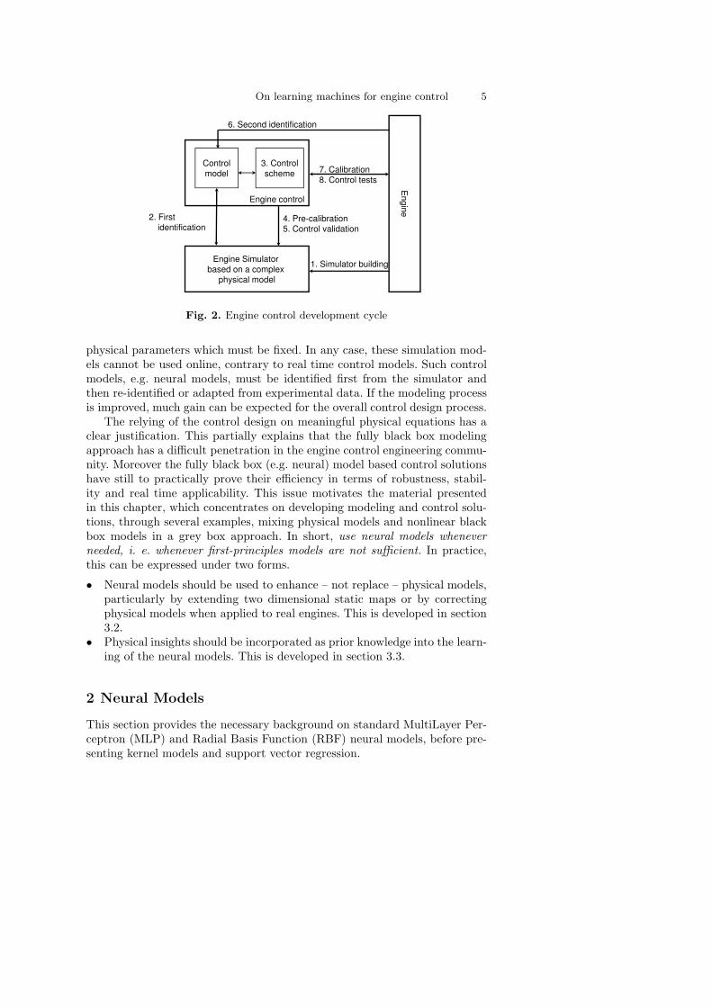
Let us now focus on the development cycle of engine control, presented inFigure 2, and the different models that are used in this framework. The designprocess is the following:

1. Building of an engine simulator mostly based on prior knowledge,2. First identification of control models from data provided by the simulator,3. Control scheme design,4. Simulation and pre-calibration of the control scheme with the simulator,5. Control validation with the simulator,6. Second identification of control models from data gathered on the engine,7. Calibration and final test of the control with the engine.

This shows that, in current practice, more or less complex simulation environ-ments based on physical relations are built for internal combustion engines.The great amount of knowledge that is included is consequently available.These simulators are built to be accurate, but this accuracy depends on many


6 S d id tifi ti

3 ControlControl

6. Second identification

En

g

3. Control

scheme

Control

model

Engine control

7. Calibration

8. Control tests

ine

2. First

identification4. Pre-calibration

5. Control validation

1. Simulator buildingEngine Simulator

based on a complex

physical model

Fig. 2. Engine control development cycle

physical parameters which must be fixed. In any case, these simulation mod-els cannot be used online, contrary to real time control models. Such controlmodels, e.g. neural models, must be identified first from the simulator andthen re-identified or adapted from experimental data. If the modeling processis improved, much gain can be expected for the overall control design process.

The relying of the control design on meaningful physical equations has aclear justification. This partially explains that the fully black box modelingapproach has a difficult penetration in the engine control engineering commu-nity. Moreover the fully black box (e.g. neural) model based control solutionshave still to practically prove their efficiency in terms of robustness, stabil-ity and real time applicability. This issue motivates the material presentedin this chapter, which concentrates on developing modeling and control solu-tions, through several examples, mixing physical models and nonlinear blackbox models in a grey box approach. In short, use neural models whenever

needed, i. e. whenever first-principles models are not sufficient. In practice,this can be expressed under two forms.

• Neural models should be used to enhance – not replace – physical models,particularly by extending two dimensional static maps or by correctingphysical models when applied to real engines. This is developed in section3.2.

• Physical insights should be incorporated as prior knowledge into the learn-ing of the neural models. This is developed in section 3.3.

2 Neural Models

This section provides the necessary background on standard MultiLayer Per-ceptron (MLP) and Radial Basis Function (RBF) neural models, before pre-senting kernel models and support vector regression.


2.1 Two neural networks

As depicted in [45], a general neural model with a single output may be writtenas a function expansion of the form

f(ϕ, θ) =

n∑

k=1

αkgk(ϕ) + α0 , (1)

where ϕ = [ϕ1 . . . ϕi . . . ϕp]T is the regression vector and θ is the parameter

vector.The restriction of the multilayer perceptron to only one hidden layer and

to a linear activation function at the output corresponds to a particular choice,the sigmoid function, for the basis function gk, and to a ”ridge” constructionfor the inputs in model (1). Although particular, this model will be calledMLP in this chapter. Its form is given, for a single output fnn, by

fnn(ϕ, θ) =

n∑

k=1

w2k g

p∑

j=1

w1kjϕj + b1

k

+ b2, (2)

where θ contains all the weights w1kj and biases b1

k of the n hidden neurons

together with the weights and bias w2k, b2 of the output neuron, and where

the activation function g is a sigmoid function (often the hyperbolic tangentg(x) = 2/(1 + e−2x) − 1).

On the other hand, choosing a Gaussian function g(x) = exp(

−x2/σ2)

as basis function and a radial construction for the inputs leads to the radialbasis function network (RBFN) [37], of which the output is given by

f(ϕ, θ) =n

∑

k=1

αkg (‖ϕ − γk‖σk) + α0 (3)

=

n∑

k=1

αk exp

−1

2

p∑

j=1

(ϕj − γkj)2

σ2kj

+ α0 ,

where γk = [γk1 . . . γkp]T is the ”center” or ”position” of the kth Gaussian

and σk = [σk1 . . . σkp]T its ”scale” or ”width”, most of the time with σkj =

σk, ∀j, or even σkj = σ, ∀j, k.The process of approximating nonlinear relationships from data with these

models can be decomposed in several steps:

• determining the structure of the regression vector ϕ or selecting the inputsof the network, see e.g. [44] for dynamic system identification;

• choosing the nonlinear mapping f or, in the neural network terminology,selecting an internal network architecture, see e.g. [40] for MLP’s pruningor [36] for RBFN’s center selection;


• estimating the parameter vector θ, i.e., (weight) ”learning” or ”training”;• validating the model.

This approach is similar to the classical one for linear system identification[28], the selection of the model structure being, nevertheless, more involved.For a more detailed description of the training and validation procedures, see[6] or [35].

Among the numerous nonlinear models, neural or not, which can be usedto estimate a nonlinear relationship, the advantages of the one hidden layerperceptron, as well as those of the radial basis function network, can be sum-marized as follows: they are flexible and parsimonious nonlinear black box

models, with universal approximation capabilities [5].

2.2 Kernel expansion models and Support Vector Regression

In the past decade, kernel methods [42] have attracted much attention in alarge variety of fields and applications: classification and pattern recognition,regression, density estimation. . . Indeed, using kernel functions, many linearmethods can be extended to the nonlinear case in an almost straightforwardmanner, while avoiding the curse of dimensionality by transposing the focusfrom the data dimension to the number of data. In particular, Support VectorRegression (SVR), stemming from statistical learning theory [50] and basedon the same concepts as the Support Vector Machine (SVM) for classifica-tion, offers an interesting alternative both for nonlinear modeling and systemidentification [15, 32, 52].

SVR originally consists in finding the kernel model that has at most a devi-ation ε from the training samples with the smallest complexity [46]. Thus, SVRamounts to solving a constrained optimization problem known as a quadraticprogram (QP), where both the ℓ1-norm of the errors larger than ε and theℓ2-norm of the parameters are minimized. Other formulations of the SVRproblem minimizing the ℓ1-norm of the parameters can be derived to yieldlinear programs (LP) [47, 30]. Some advantages of this latter approach canbe noticed compared to the QP formulation such as an increased sparsity ofsupport vectors or the ability to use more general kernels [29]. The remainingof this chapter will thus focus on the LP formulation of SVR (LP-SVR).

Nonlinear mapping and kernel functions

A kernel model is an expansion of the inner products by the N trainingsamples xi ∈ IRp mapped in a higher dimensional feature space. Defining thekernel function k(x,xi) = Φ(x)T Φ(xi), where Φ(x) is the image of the pointx in that feature space, allows to write the model as a kernel expansion

f(x) =

N∑

i=1

αik(x,xi) + b = K(x,XT )α + b , (4)


where α = [α1 . . . αi . . . αN ]T and b are the parameters of the model, thedata (xi, yi), i = 1, . . . , N , are stacked as rows in the matrix X ∈ IRN×p andthe vector y, and K(x,XT ) is a vector defined as follows. For A ∈ Rp×m andB ∈ Rp×n containing p-dimensional sample vectors, the “kernel” K(A,B)maps Rp×m ×Rp×n in Rm×n with K(A,B)i,j = k(Ai,Bj), where Ai and Bj

are the ith and jth columns of A and B. Typical kernel functions are thelinear (k(x,xi) = xTxi), Gaussian RBF (k(x,xi) = exp(−‖x − xi‖

22/2σ2) )

and polynomial (k(x,xi) = (xT xi + 1)d) kernels. The kernel function definesthe feature space F in which the data are implicitly mapped. The higher thedimension of F , the higher the approximation capacity of the function f , upto the universal approximation capacity obtained for an infinite feature space,as with Gaussian RBF kernels.

Support Vector Regression by Linear Programming

In Linear Programming Support Vector Regression (LP-SVR), the model com-plexity, measured by the ℓ1-norm of the parameters α, is minimized togetherwith the error on the data, measured by the ε-insensitive loss function l,defined by [50] as

l(yi − f(xi)) =

{

0 if |yi − f(xi)| ≤ ε ,

|yi − f(xi)| − ε otherwise .(5)

Minimizing the complexity of the model allows to control its generalizationcapacity. In practice, this amounts to penalizing non-smooth functions andimplements the general smoothness assumption that two samples close ininput space tend to give the same output.

Following the approach of [30], two sets of optimization variables, in twopositive slack vectors a and ξ, are introduced to yield a linear program solvableby standard optimization routines such as the MATLAB linprog function. Inthis scheme, the LP-SVR problem may be written as

min(α,b,ξ≥0,a≥0)

1T a + C1T ξ

s.t. −ξ ≤ K(X,XT )α + b1− y ≤ ξ

0 ≤ 1ε ≤ ξ

−a ≤ α ≤ a ,

(6)

where a hyperparameter C is introduced to tune the trade-off between theminimization of the model complexity and the minimization of the error. Thelast set of constraints ensures that 1Ta, which is minimized, bounds ‖α‖1. Inpractice, sparsity is obtained as a certain number of parameters αi will tendto zero. The input vectors xi for which the corresponding αi are non-zero arecalled support vectors (SVs).


2.3 Link between Support Vector Regression and RBFNs

For a Gaussian kernel, the kernel expansion (4) can be interpreted as a RBFNwith N neurons in the hidden layer centered at the training samples xi andwith a unique width σk = [σ . . . σ]T , k = 1, . . . , N . Compared to neuralnetworks, SVR has the following advantages: automatic selection and sparsityof the model, intrinsic regularization, no local minima (convex problem witha unique solution), and good generalization ability from a limited amount ofsamples.

It seems though that least squares estimates of the parameters or standardRBFN training algorithms are most of the time satisfactory, particularly whena sufficiently large number of samples corrupted by Gaussian noise is available.Moreover, in this case, standard center selection algorithms may be fasterand yield a sparser model than SVR. However, in difficult cases, the goodgeneralization capacity and the better behavior with respect to outliers ofSVR may help. Even if non-quadratic criteria have been proposed to train [8]or prune neural networks [49, 24], the SVR loss function is intrinsically robustand thus allows accommodation to non-Gaussian noise probability densityfunctions. In practice, it is advised to employ SVR in the following cases.

• Few data are available.• The noise is non-Gaussian.• The training set is corrupted by outliers.

Finally, the computational framework of SVR allows for easier extensions suchas the one described in this chapter, namely, the inclusion of prior knowledge.

3 Engine control applications

3.1 Introduction

The application treated here, the control of the turbocharged Spark Ignitionengine with Variable Camshaft Timing, is representative of modern enginecontrol problems. Indeed, such an engine presents for control the commoncharacteristics mentioned in the introduction 1.1 and comprises several airactuators and therefore several degrees of freedom for airpath control.

More stringent standards are being imposed to reduce fuel consumptionand pollutant emissions for Spark Ignited (SI) engines. In this context, down-sizing appears as a major way for reducing fuel consumption while maintainingthe advantage of low emission capability of three-way catalytic systems andcombining several well known technologies [27]. (Engine) downsizing is theuse of a smaller capacity engine operating at higher specific engine loads,i.e. at better efficiency points. In order to feed the engine, a well-adaptedturbocharger seems to be the best solution. Unfortunately, the turbochargerinertia involves long torque transient responses [27]. This problem can be


partially solved by combining turbocharging and Variable Camshaft Timing(VCT) which allows air scavenging from the intake to the exhaust.

pman

Tman

Sthr

WG

Qcyl

Qthr

VCTexhVCTin

Lambda sensor

turbine

compressor

Manifold

pint

pamb

Tamb

Fig. 3. Airpath of a Turbocharged SI Engine with VCT

The air intake of a turbocharged SI Engine with VCT, represented inFigure 3, can be described as follows. The compressor (pressure pint) producesa flow from the ambient air (pressure pamb and temperature Tamb). This airflow Qth is adjusted by the intake throttle (section Sth) and enters the intakemanifold (pressure pman and temperature Tman). The flow that goes into thecylinders Qcyl passes through the intake valves, whose timing is controlled bythe intake Variable Camshaft Timing V CTin actuator. After the combustion,the gases are expelled into the exhaust manifold through the exhaust valve,controlled by the exhaust Variable Camshaft Timing V CTexh actuator. Theexhaust flow is split into turbine flow and wastegate flow. The turbine flowpowers up the turbine and drives the compressor through a shaft. Thus, thesupercharged pressure pint is adjusted by the turbine flow which is controlledby the wastegate WG.

The effects of Variable Camshaft Timing (VCT) can be summarized asfollows. On the one hand, cam timing can inhibit the production of nitrogenoxides (NOx). Indeed, by acting on the cam timing, combustion productswhich would otherwise be expelled during the exhaust stroke are retained in


the cylinder during the subsequent intake stroke. This dilution of the mix-ture in the cylinder reduces the combustion temperature and limits the NOx

formation. Therefore, it is important to estimate and control the back-flowof burned gases in the cylinder. On the other hand, with camshaft timing,air scavenging can appear, that is air passing directly from the intake to theexhaust through the cylinder. For that, the intake manifold pressure mustbe greater than the exhaust pressure when the exhaust and intake valvesare opened together. In that case, the engine torque dynamic behavior is im-proved, i.e. the settling times decreased. Indeed, the flow which passes throughthe turbine is increased and the corresponding energy is transmitted to thecompressor. In transient, it is also very important to estimate and control thisscavenging for torque control.

For such an engine, the following presents the inclusion of neural modelsin various modeling and control schemes in two parts: an air path controlbased on an in-cylinder air mass observer, and an in-cylinder residual gasestimation. In the first example, the air mass observer will be necessary tocorrect the manifold pressure set point. The second example deals with theestimation of residual gases for a single cylinder naturally-aspirated engine.In this type of engine, no scavenging appears, so that estimation of burnedgases and air scavenging of the first example is simplified into a residual gasestimation.

3.2 Airpath observer based control

Control scheme

The objective of engine control is to supply the torque requested by the driverwhile minimizing the pollutant emissions. For a SI engine, the torque is di-rectly linked to the air mass trapped in the cylinder for a given engine speedNe and an efficient control of this air mass is then required. The air path con-trol, i.e. throttle, turbocharger and variable camshaft timing (VCT) control,can be divided in two main parts: the air mass control by the throttle and theturbocharger and the control of the gas mix by the variable camshaft timing(see [11] for further details on VCT control). The structure of the air masscontrol scheme, described in figure 4, is now detailed block by block. Thesupervisor, that corresponds to a part of the Combustion layer of figure 1,builds the in-cylinder air mass set point from the indicated torque set point,computed by the Engine layer. The determination of manifold pressure setpoints is presented at the end of the section. The general control structureuses an in-cylinder air mass observer discussed below that corrects the errorsof the manifold pressure model. The remaining blocks are not described inthis chapter but an Internal Model Control (IMC) of the throttle is proposedin [11] and a linearized neural Model Predictive Control (MPC) of the tur-bocharger can be found in [10, 11]. The IMC scheme relies on a grey boxmodel, which includes a neural static estimator. The MPC scheme is basedon a dynamical neural model of the turbocharger.


(Set point) Turbocharger(Sensors)

WG(Set point)

( p )Manifoldpressure

model

Control(Sensors)

-+_air spm

_man spp

thS

, ,man e int

p N p

Air P

a

Superv

Torque Set

ThrottleControl

(Sensors)

th

manp

ath

vis

or

SetPoint

im

(Sensors)

, , ,e in exh manN VCT VCT T

Air mass observer

ˆairm

_air spm

(Sensors)

, ,man ep N

VCT VCT, ,in exh

man

VCT VCT

T

EnergyLayer

ActuatorLayer

CombustionLayer

Fig. 4. General control scheme

Observation scheme

Here two nonlinear estimators of the air variables, recirculated gas mass RGMand in-cylinder air mass mair, are presented. Because these variables are notmeasured, data provided by a complex but accurate high frequency enginesimulator [26] are used to build the corresponding models.

Because scavenging and burned gas back-flow correspond to associatedflow phenomena, only one variable, the Recirculated Gas Mass (RGM), isdefined:

RGM =

{

mbg , if mbg > msc

−msc , otherwise,(7)

where mbg is the in-cylinder burned gas mass and msc is the scavenged airmass. Note that, when scavenging from the intake to the exhaust occurs, theburned gases are insignificant. The recirculated gas mass RGM estimator isa neural model entirely obtained from the simulated data.

Considering in-cylinder air mass observation, a lot of references are avail-able especially for air-fuel ratio (AFR) control in a classical engine [20]. Morerecently, [48] uses an ”input observer” to determine the engine cylinder flowand [3] uses a Kalman filter to reconstruct the air mass for a turbocharged SIengine.

A novel observer for the in-cylinder air mass mair is presented below.Contrary to the references above, it takes into account a non measured phe-nomenon (scavenging), and can thus be applied with advanced engine tech-nology (turbocharged VCT engine). Moreover, its on-line computational load


is low. As presented in Figure 5, this observer combines open loop nonlin-

manp

Observer (17)

thQ

RGM

Air Flow meter +-ˆ

manp

Q Observer (17)

based on (11)manp

eN

inVCT

RGM

cylQ

(13)air

mˆcyl

Q

(12)RGM estimator (8)sc

Q

(18)

exhVCT Volumetric efficiency

estimator (10)

vol

manT

_air OLm

ˆ

++

Open loop

air mass

estimator (9)

_air cylm

Fig. 5. Air mass observer scheme

ear neural based statical estimators of RGM and mair, and a ”closed loop”polytopic observer. The observer is built from the Linear Parameter Varyingmodel of the intake manifold and dynamically compensates for the residualerror ∆Qcyl committed by one of the estimators, based on a principle similarto the one presented in [2].

Open loop estimators

Recirculated gas mass model

Studying the RGM variable (7) is complex because it cannot be measuredon-line. Consequently, a static model is built from data provided by the enginesimulator. The perceptron with one hidden layer and a linear output unit (2)is chosen with a hyperbolic tangent activation function g.

The choice of the regressors ϕj is based on physical considerations and the

estimated Recirculated Gas Mass RGM is given by

RGM = fnn(pman, Ne, V CTin, V CTexh), (8)

where pman is the intake manifold pressure, Ne the engine speed, V CTin theintake camshaft timing, and V CTexh the exhaust camshaft timing.

Open loop air mass estimator

The open loop model mair OL of the in-cylinder air mass is based on thevolumetric efficiency equation:


mair OL = ηvol

pambVcyl

rTman

, (9)

where Tman is the manifold temperature, pamb the ambient pressure, Vcyl thedisplacement volume, r the perfect gas constant, and where the volumetricefficiency ηvol is described by the static nonlinear function f of four variables:pman, Ne, V CTin and V CTexh.

In [14], various black box models, such as polynomial, spline, MLPand RBFN models, are compared for the static prediction of the volu-metric efficiency. In [9], three models of the function f , obtained fromengine simulator data, are compared: a polynomial model linear in man-ifold pressure proposed by Jankovic [22] f1(Ne, V CTin, V CTexh)pman +f2(Ne, V CTin, V CTexh), where f1 et f2 are 4th order polynomials, completewith 69 parameters, then reduced by stepwise regression to 43 parameters;a standard 4th order polynomial model f3(pman, Ne, V CTin, V CTexh), com-plete with 70 parameters then reduced to 58 parameters; and a MLP modelwith 6 hidden neurons (37 parameters)

ηvol = fnn(pman, Ne, V CTin, V CTexh) . (10)

Training of the neural model has been performed by minimizing the meansquared error, using the Levenberg-Marquardt algorithm. The behavior ofthese models is similar, and the most important errors are committed at thesame operating points. Nevertheless, the neural model, that involves the small-est number of parameters and yields slightly better approximation results, ischosen as the static model of the volumetric efficiency. These results illustratethe parsimony property of the neural models.

Air mass observer

Principle

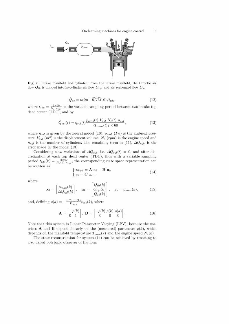
The air mass observer is based on the flow balance in the intake manifold.As shown in figure 3.2, a flow Qth enters the manifold and two flows leaveit: the flow that is captured in the cylinder Qcyl and the flow scavenged fromthe intake to the exhaust Qsc. The flow balance in the manifold can thus bewritten as

pman(t) =rTman(t)

Vman

(Qth(t) − Qcyl(t) − ∆Qcyl(t) − Qsc(t)) , (11)

where, for the intake manifold, pman is the pressure to be estimated (in Pa),Tman is the temperature (K), Vman is the volume (m3), supposed to be con-stant and r is the ideal gas constant. In (11), Qth can be measured by anair flow meter (kg/s). On the other hand, Qsc (kg/s) and Qcyl (kg/s) are

respectively estimated by differentiating the Recirculated Gas Mass RGM(8):


pman

pint

Qth

Q

Qcyl

Qsc

Fig. 6. Intake manifold and cylinder. From the intake manifold, the throttle airflow Qth is divided into in-cylinder air flow Qcyl and air scavenged flow Qsc

Qsc = min(−RGM, 0)/ttdc, (12)

where ttdc = 2×60Ne ncyl

is the variable sampling period between two intake top

dead center (TDC), and by

Qcyl(t) = ηvol(t)pamb(t) Vcyl Ne(t) ncyl

rTman(t)2 × 60, (13)

where ηvol is given by the neural model (10), pamb (Pa) is the ambient pres-sure, Vcyl (m3) is the displacement volume, Ne (rpm) is the engine speed andncyl is the number of cylinders. The remaining term in (11), ∆Qcyl, is theerror made by the model (13).

Considering slow variations of ∆Qcyl, i.e. ∆Qcyl(t) = 0, and after dis-cretization at each top dead center (TDC), thus with a variable samplingperiod ttdc(k) = 2×60

Ne(k) ncyl, the corresponding state space representation can

be written as{

xk+1 = A xk + B uk

yk = C xk ,(14)

where

xk =

[

pman(k)∆Qcyl(k)

]

, uk =

Qth(k)Qcyl(k)Qsc(k)

, yk = pman(k), (15)

and, defining ρ(k) = − r Tman(k)Vman

ttdc(k), where

A =

[

1 ρ(k)0 1

]

, B =

[

−ρ(k) ρ(k) ρ(k)0 0 0

]

. (16)

Note that this system is Linear Parameter Varying (LPV), because the ma-trices A and B depend linearly on the (measured) parameter ρ(k), whichdepends on the manifold temperature Tman(k) and the engine speed Ne(k).

The state reconstruction for system (14) can be achieved by resorting toa so-called polytopic observer of the form


{

xk+1 = A(ρk)xk + B(ρk)uk + K(yk − yk)yk = Cxk ,

(17)

with a constant gain K.This gain is obtained by solving a Linear Matrix Inequality (LMI). This

LMI ensures the convergence towards zero of the reconstruction error for thewhole operating domain of the system based on its polytopic decomposition.This ensures the global convergence of the observer. See [34], [33] and [13] forfurther details.

Then, the state ∆Qcyl is integrated (i.e. multiplied by ttdc) to give the airmass bias

∆mair = ∆Qcyl × ttdc . (18)

Finally, the in-cylinder air mass can be estimated by correcting the open loopestimator (9) with this bias as

mair cyl = mair OL + ∆mair . (19)

Results

Some experimental results, normalized between 0 and 1, obtained on a 1.8Liter turbocharged 4 cylinder engine with Variable Camshaft Timing are givenin figure 7. A measurement of the in-cylinder air mass, only valid in steady

28 30 32 34 36 38 40 420.05

0.1

0.15

0.2

0.25

0.3

0.35

0.4

0.45

0.5

Time (s)

Normalised air mass

MeasurementObserver without neural modelOpen Loop neural modelNeural based observer

Fig. 7. Air mass observer results (mg) vs. time (s) on an engine test bench


state, can be obtained from the measurement of Qth by an air flow meter.Indeed, in steady state with no scavenging, the air flow that gets into thecylinder Qcyl is equal to the flow that passes through the throttle Qth (seeFigure 3.2). In consequence, this air mass measurement is obtained by inte-grating Qth (i.e. multiplying by ttdc). Figure 7 compares this measurement,the open loop neural estimator ((9) with a neural model (10)), an estimationnot based on this neural model (observer (17) based on model (11) but withQcyl = Qsc = 0), the proposed estimation ((19) combining the open loop neu-ral estimator (9) and the polytopic observer (17) based on model (11) withQcyl given by (13) using the neural model (10) and Qsc given by (12) using(8)).

For steps of air flow, the open loop neural estimator tracks very quickly themeasurement changes, but a small steady state error can be observed (see forexample between 32 s and 34 s). Conversely, the closed loop observer whichdoes not take into account this feedforward estimator involves a long transienterror while guarantying the convergence in steady state. Finally, the proposedestimator, including feedforward statical estimators and a polytopic observer,combines both the advantages: very fast tracking and no steady state error.This observer can be used to design and improve the engine supervisor offigure 5 by determining the air mass set points.

Computing the manifold pressure set points

To obtain the desired torque of a SI engine, the air mass trapped in thecylinder must be precisely controlled. The corresponding measurable variableis the manifold pressure. Without Variable Camshaft Timing (VCT), thisvariable is linearly related to the trapped air mass, whereas with VCT, thereis no more one-to-one correspondence. Figure 8 shows the relationship betweenthe trapped air mass and the intake manifold pressure at three particular VCTpositions for a fixed engine speed.

Thus, it is necessary to model the intake manifold pressure pman. Thechosen static model is a perceptron with one hidden layer (2). The regressorshave been chosen from physical considerations: air mass mair (corrected bythe intake manifold temperature Tman), engine speed Ne, intake V CTin andexhaust V CTexh camshaft timing. The intake manifold pressure model is thusgiven by

pman = fnn (mair, Ne, V CTin, V CTexh) . (20)

Training of the neural model from engine simulator data has been performedby minimizing the mean squared error, using the Levenberg-Marquardt algo-rithm.

The supervisor gives an air mass set point mair sp from the torque setpoint (figure 4). The intake manifold pressure set point, computed by model(20), is corrected by the error ∆mair (18) to yield the final set point pman sp

aspman sp = fnn (mair sp − ∆mair sp, Ne, V CTin, V CTexh) . (21)


100 150 200 250 300 350 4000.2

0.3

0.4

0.5

0.6

0.7

0.8

0.9

1

Air mass (mg)

Manifold pressure (bar)

VCTin

=0, VCTexh

=0

VCTin

=40, VCTexh

=40

VCTin

=0, VCTexh

=20

Fig. 8. Relationship between the manifold pressure (in bar) and the air masstrapped (in mg) for a SI engine with VCT at 2000 rpm

Engine test bench results

The right part of figure 9 shows an example of results for air mass control, inwhich the VCT variations are not taken into account. Considerable air massvariations (nearly ±25% of the set point) can be observed. On the contrary,the left part shows the corresponding results for the proposed air mass control.The air mass is almost constant (nearly ±2% of variation), illustrating that themanifold pressure set point is well computed with (21). This allows to reducethe pollutant emissions without degrading the torque set point tracking.

3.3 Estimation of in-cylinder residual gas fraction

The application deals with the estimation of residual gases in the cylinders ofSpark Ignition (SI) engines with Variable Camshaft Timing (VCT) by SupportVector Regression (SVR) [7]. More precisely, we are interested in estimatingthe residual gas mass fraction by incorporating prior knowledge in the SVRlearning with the general method proposed in [25]. Knowing this fractionallows to control torque as well as pollutant emissions. The residual gas massfraction χres can be expressed as a function of the engine speed Ne, theratio pman/pexh, where pman and pexh are respectively the (intake) manifoldpressure and the exhaust pressure, and an overlapping factor OF (in ◦/m)[16], related to the time during which the valves are open together.

The available data are provided, on one hand, from the modeling and simu-lation environment Amesim [21], which uses a high frequency zero-dimensional


0 10 20 30 40 50 600.11

0.12

0.12

0.14

0.15

0.16

0.17Normalised Air Mass

Time (s)

Set pointObservation

0 5 10 15 20 25 30 35 400.1

0.11

0.12

0.13

0.14

0.15

0.16

0.17Normalised Air Mass

Time (s)

Set PointObservation

Fig. 9. Effect of the variation of VCT’s on air mass with the proposed controlscheme (left) and without taking into account the variation of VCT’s in the controlscheme (right)

thermodynamic model and, on the other hand, from off line measurements,which are accurate, but complex and costly to obtain, by direct in-cylindersampling [18]. The problem is this. How to obtain a simple, embeddable, blackbox model with a good accuracy and a large validity range for the real engine,from precise real measurements as less numerous as possible and a represen-tative, but possibly biased, prior simulation model? The problem thus posed,although particular, is very representative of numerous situations met in en-gine control, and more generally in engineering, where complex models, moreor less accurate, exist and where the experimental data which can be used forcalibration are difficult or expensive to obtain.

The simulator being biased but approximating rather well the overall shapeof the function, the prior knowledge will be incorporated in the derivatives.Prior knowledge of the derivatives of a SVR model can be enforced in thetraining by noticing that the kernel expansion (4) is linear in the parametersα, which allows to write the derivative of the model output with respect tothe scalar input xj as

∂f(x)

∂xj=

N∑

i=1

αi

∂k(x,xi)

∂xj= rj(x)T α , (22)

where rj(x) = [∂k(x,x1)/∂xj . . . ∂k(x,xi)/∂xj . . . ∂k(x,xN )/∂xj]T is ofdimension N . The derivative (22) is linear in α. In fact, the form of thekernel expansion implies that the derivatives of any order with respect to anycomponent are linear in α. Prior knowledge of the derivatives can thus beformulated as linear constraints.

The proposed model is trained by a variant of algorithm (6) with additionalconstraints on the derivatives at the points xp of the simulation set. In thecase where the training data do not cover the whole input space, extrapolationoccurs, which can become a problem when using local kernels such as theRBF kernel. To avoid this problem, the simulation data xp, p = 1, . . . , Npr,


are introduced as potential support vectors (SVs). The resulting global modelis now

f(x) = K(x, [XT XT])α + b , (23)

where α ∈ IRN+Npr

and [XT XT] is the concatenation of the matrices XT =

[x1 . . . xi . . . xN ], containing the real data, and XT

= [x1 . . . xp . . . xNpr ],containing the simulation data. Defining the Npr × (N + Npr)-dimensional

matrix R(XT, [XT X

T]) = [r1(x1) . . . r1(xp) . . . r1(xNpr)]T , where r1(x)

corresponds to the derivative of (23) with respect to the input x1 = pman/pexh,the proposed model is obtained by solving

min(α,b,ξ,a,z)

1

N + Npr1Ta +

C

N1T ξ +

λ

Npr1T z

s.t. −ξ ≤ K(XT , [XT XT])α + b1− y ≤ ξ

0 ≤ 1ε ≤ ξ

−a ≤ α ≤ a

−z ≤ R(XT, [XT X

T])α − y′ ≤ z ,

(24)

where y′ contains the Npr known values of the derivative with respect tothe input pman/pexh, at the points xp of the simulation set. In order to

be able to evaluate these values, a prior model, f(x) =∑Npr

p=1 αpk(x, xp) +

b, is first trained on the Npr simulation data (xp, yp), p = 1, . . . , Npr,only. This prior model is then used to provide the prior derivatives y′ =[∂f(x1)/∂x1 . . . ∂f(xp)/∂x1 . . . ∂f(xNpr)/∂x1]T .

Note that the knowledge of the derivatives is included by soft constraints,thus allowing to tune the trade-off between the data and the prior knowledge.The weighting hyperparameters are set to C/N and λ/Npr in order to main-tain the same order of magnitude between the regularization, error and priorknowledge terms in the objective function. This allows to ease the choice of Cand λ based on the application goals and confidence in the prior knowledge.Hence, the hyperparameters become problem independent.

The method is now evaluated on the in-cylinder residual gas fraction ap-plication. In this experiment, three data sets are built from the available datacomposed of 26 experimental samples plus 26 simulation samples:

• the training set (X,y) composed of a limited amount of real data (Nsamples),

• the test set composed of independent real data (26 − N samples),• the simulation set (X, y) composed of data provided by the simulator

(Npr = 26 samples).

The test samples are assumed to be unknown during the training and areretained for testing only. It must be noted that the inputs of the simulationdata do not exactly coincide with the inputs of the experimental data as shownin Figure 3.3 for N = 3.


0.4 0.6 0.8 10

10

20

30

0.4 0.6 0.8 10

10

20

30

0.4 0.6 0.8 10

10

20

30

0.4 0.6 0.8 10

10

20

30

0.4 0.6 0.8 10

10

20

30

0.4 0.6 0.8 10

10

20

30

Ne = 1000 rpmOF = 0◦CA/m

OF = 0.41◦CA/m

OF = 1.16◦CA/m

Ne = 2000 rpmOF = 0.58◦CA/m

OF = 1.16◦CA/m

OF = 2.83◦CA/m

Fig. 10. Residual gas mass fraction χres in percentages as a function of the ratiopman/pexh for two engine speeds Ne and different overlapping factors OF . The 26experimental data are represented by plus signs (+) with a superposed circle (⊕) forthe 3 points retained as training samples. The 26 simulation data appear as asterisks(∗)

The comparison is performed between four models.

• The experimental model trained by (6) on the real data set (X,y) only,• the prior model trained by (6) on the simulation data (X, y) only,• the mixed model trained by (6) on the real data set simply extended with

the simulation data ([XT XT]T , [yT yT ]T ) (the training of this model is

close in spirit to the virtual sample approach, where extra data are addedto the training set),

• the proposed model trained by (24) and using both the real data (X,y)and the simulation data (X, y).

These models are evaluated on the basis of three indicators: the root meansquare error (RMSE) on the test set (RMSE test), the RMSE on all exper-imental data (RMSE) and the maximum absolute error on all experimentaldata (MAE).


Before training, the variables are normalized with respect to their meanand standard deviation. The different hyperparameters are set according tothe following heuristics. One goal of the application is to obtain a model thatis accurate on both the training and test samples (the training points are partof the performance index RMSE). Thus C is set to a large value (C = 100) inorder to ensure a good approximation of the training points. Accordingly, ε isset to 0.001 in order to approximate the real data well. The trade-off parameterλ of the proposed method is set to 100, which gives as much weight to boththe training data and the prior knowledge. Since all standard deviations ofthe inputs are equal to 1 after normalization, the RBF kernel width σ is setto 1.

Table 1. Errors on the residual gas mass fraction with the number of real andsimulation data used for training. ’–’ appears when the result is irrelevant (modelmostly constant).

Model # of realdata N

# of simula-tion data Npr

RMSE test RMSE MAE

experimental model 6 6.84 6.00 15.83prior model 26 4.86 4.93 9.74mixed model 6 26 4.85 4.88 9.75proposed model 6 26 2.44 2.15 5.94

experimental model 3 – – –prior model 26 4.93 4.93 9.74mixed model 3 26 4.89 4.86 9.75proposed model 3 26 2.97 2.79 5.78

Two sets of experiments are performed for very low numbers of trainingsamples N = 6 and N = 3. The results in Table 1 show that both the exper-

imental and the mixed models cannot yield a better approximation than theprior model with so few training data. Moreover, for N = 3, the experimental

model yields a quasi-constant function due to the fact that the model hasnot enough free parameters (only 3 plus a bias term) and thus cannot modelthe data. In this case, the RMSE is irrelevant. On the contrary, the proposed

model does not suffer from a lack of basis functions, thanks to the inclusionof the simulation data as potential support vectors. This model yields goodresults from very few training samples. Moreover, the performance decreasesonly slightly when reducing the training set size from 6 to 3. Thus, the pro-posed method seems to be a promising alternative to obtain a simple blackbox model with a good accuracy from a limited number of experimental dataand a prior simulation model.


4 Conclusion

The chapter exposed learning machines for engine control applications. Thetwo neural models most used in modeling for control, the MultiLayer Per-ceptron and the Radial Basis Function network, have been described, alongwith a more recent approach, known as Support Vector Regression. The useof such black box models has been placed in the design cycle of engine control,where the modeling steps constitute the bottleneck of the whole process. Ap-plication examples have been presented for a modern engine, a turbochargedSpark Ignition engine with Variable Camshaft Timing. In the first example,the airpath control was studied, where open loop neural estimators are com-bined with a dynamical polytopic observer. The second example consideredmodeling a variable which is not measurable on-line, from a limited amountof experimental data and a simulator built from prior knowledge.

The neural black box approach for modeling and control allows to developgeneric, application independent, solutions. The price to pay is the loss of thephysical interpretability of the resulting models. Moreover, the fully black box(e.g. neural) model based control solutions have still to practically prove theirefficiency in terms of robustness or stability. On the other hand, models basedon first principles (white box models) are completely meaningful and manycontrol approaches with good properties have been proposed, which are wellunderstood and accepted in the engine control community. However, thesemodels are often inadequate, too complex or too difficult to parametrize, asreal time control models. Therefore, intermediate solutions, involving grey boxmodels, seem to be preferable for engine modeling, control and, at a higherlevel, optimization. In this framework, two approaches can be considered.First, beside first principles models, black box neural sub-models are chosenfor variables difficult to model (e.g. volumetric efficiency, pollutant emissions).Secondly, black box models can be enhanced thanks to physical knowledge.The examples presented in this chapter showed how to implement these greybox approaches in order to obtain efficient and acceptable results.

References

1. C. Alippi, , C. De Russis, and V. Piuri. A neural-network based control solutionto air fuel ratio for automotive fuel injection system. IEEE Trans. on SystemMan and Cybernetics - Part C, 33(2):259–268, 2003.

2. P. Andersson. Intake Air Dynamics on a Turbocharged SI Engine with Waste-gate. PhD thesis, Linkoping University, Sweden, 2002.

3. P. Andersson and L. Eriksson. Mean-value observer for a turbocharged SI en-gine. In Proc. of the IFAC Symp. on Advances in Automotive Control, Salerno,Italy, pages 146–151, April 2004.

4. I. Arsie, C. Pianese, and M. Sorrentino. A procedure to enhance identificationof recurrent neural networks for simulating air-fuel ratio dynamics in SI engines.Engineering Applications of Artificial Intelligence, 19(1):65–77, 2006.


5. A. R. Barron. Universal approximation bounds for superpositions of a sigmoidalfunction. IEEE Trans. on Information Theory, 39(3):930–945, 1993.

6. G. Bloch. and T. Denoeux. Neural networks for process control and optimiza-tion: two industrial applications. ISA Transactions, 42(1):39–51, 2003.

7. G. Bloch, F. Lauer, G. Colin, and Y. Chamaillard. Combining experimentaldata and physical simulation models in support vector learning. In L. Iliadisand K. Margaritis, editors, Proc. of the 10th Int. Conf. on Engineering Applica-tions of Neural Networks (EANN), Thessaloniki, Greece, volume 284 of CEURWorkshop Proceedings, pages 284–295, 2007.

8. G. Bloch, F. Sirou, V. Eustache, and P. Fatrez. Neural intelligent control of asteel plant. IEEE Trans. on Neural Networks, 8(4):910–918, 1997.

9. G. Colin. Controle des systemes rapides non lineaires – Application au mo-teur a allumage commande turbocompresse a distribution variable. PhD thesis,University of Orleans, France, 2006.

10. G. Colin, Y. Chamaillard, G. Bloch, and A. Charlet. Exact and linearised neuralpredictive control - a turbocharged SI engine example. Journal of DynamicSystems, Measurement and Control - Trans. of the ASME, 129(4):527–533, 2007.

11. G. Colin, Y. Chamaillard, G. Bloch, and G. Corde. Neural control of fastnonlinear systems, Application to a turbocharged SI engine with VCT. IEEETrans. on Neural Networks, 18(4):1101–1114, 2007.

12. G. Corde. Le controle moteur. In G. Gissinger and N. Le Fort Piat, editors,Controle commande de la voiture. Hermes, 2002.

13. J. Daafouz and J. Bernussou. Parameter dependent Lyapunov functions fordiscrete time systems with time varying parametric uncertainties. Systems &Control Letters, 43(5):355–359, August 2001.

14. G. De Nicolao, R. Scattolini, and C. Siviero. Modelling the volumetric efficiencyof IC engines: parametric, non-parametric and neural techniques. Control En-gineering Practice, 4(10):1405–1415, 1996.

15. P.M.L. Drezet and R.F. Harrison. Support vector machines for system identifi-cation. In Proc. of the UKACC Int. Conf. on Control, Swansea, UK, volume 1,pages 688–692, 1998.

16. J. W. Fox, W. K. Cheng, and J. B. Heywood. A model for predicting residualgas fraction in spark-ignition engines. SAE Technical Papers, (931025), 1993.

17. J. Gerhardt, H. Honniger, and H. Bischof. A new approach to functionnaland software structure for engine management systems - BOSCH ME7. SAETechnical Papers, (980801), 1998.

18. P. Giansetti, G. Colin, P. Higelin, and Y. Chamaillard. Residual gas frac-tion measurement and computation. International Journal of Engine Research,8(4):347–364, 2007.

19. L. Guzzella and C.H. Onder. Introduction to Modeling and control of InternalCombustion Engine Systems. Springer, 2004.

20. E. Hendricks and J. Luther. Model and observer based control of internal com-bustion engines. In Proc. of the 1st Int. Workshop on Modeling Emissions andControl in Automotive Engines (MECA), Salerno, Italy, pages 9–20, Salerno,Italy, 2001.

21. Imagine. Amesim web site. www.amesim.com, 2006.22. M. Jankovic and S.W. Magner. Variable Cam Timing : Consequences to Au-

tomotive Engine Control Design. In Proc. of the 15th Triennial IFAC WorldCongress, Barcelona, Spain, 2002.


23. I. Kolmanovsky. Support vector machine-based determination of gasoline direct-injected engine admissible operating envelope. SAE Technical Papers, (2002-01-1301), 2002.

24. M. Lairi and G. Bloch. A neural network with minimal structure for maglevsystem modeling and control. In Proc. of the IEEE Int. Symp. on IntelligentControl / Intelligent Systems & Semiotics, Cambridge, MA, USA, pages 40–45,1999.

25. F. Lauer and G. Bloch. Incorporating prior knowledge in support vector regres-sion. Machine Learning, 2007. doi:10.1007/s10994-007-5035-5.

26. F. Le Berr, M. Miche, G. Colin, G. Le Solliec, and F. Lafossas. Modelling ofa Turbocharged SI Engine with Variable Camshaft Timing for Engine ControlPurposes. SAE Technical Paper, (2006-01-3264), 2006.

27. B. Lecointe and G. Monnier. Downsizing a Gasoline Engine Using Turbocharg-ing with Direct Injection. SAE Technical Paper, (2003-01-0542), 2003.

28. L. Ljung. System identification: Theory for the user. Prentice-Hall Inc., 2ndedition, 1999.

29. O. Mangasarian. Generalized support vector machines. In A. Smola, P. Bartlett,B. Scholkopf, and D. Schuurmans, editors, Advances in Large Margin Classifiers,pages 135–146. MIT Press, 2000.

30. O. L. Mangasarian and D. R. Musicant. Large scale kernel regression via linearprogramming. Machine Learning, 46(1-3):255–269, 2002.

31. K.A. Marko. Neural network application to diagnostics and control of vehiclecontrol systems. In R. Lippmann, J. E. Moody, and D. S. Touretzky, editors,Advances in Neural Information Processing Systems, volume 3, pages 537–543.Morgan Kaufmann, 1991.

32. D. Mattera and S. Haykin. Support vector machines for dynamic reconstructionof a chaotic system. In B. Scholkopf, C. J. C. Burges, and A. J. Smola, editors,Advances in kernel methods: support vector learning, pages 211–241. MIT Press,1999.

33. G. Millerioux, F. Anstett, and G. Bloch. Considering the attractor structureof chaotic maps for observer-based synchronization problems. Mathematics andComputers in Simulation, 68(1):67–85, February 2005.

34. G. Millerioux, L. Rosier, G. Bloch, and J. Daafouz. Bounded state reconstruc-tion error for LPV systems with estimated parameters. IEEE Trans. on Auto-matic Control, 49(8):1385–1389, August 2004.

35. O. Nelles. Nonlinear System Identification: From Classical Approaches to NeuralNetworks and Fuzzy Models. Springer-Verlag, Berlin, Germany, 2001.

36. M. J. L. Orr. Recent advances in radial basis function networks. Technicalreport, Edinburgh University, UK, 1999.

37. T. Poggio and F. Girosi. Networks for approximation and learning. Proc. IEEE,78(10):1481–1497, 1990.

38. G. V. Puskorius and L. A. Feldkamp. Parameter-based kalman filter training:theory and implementation. In S. Haykin, editor, Kalman filtering and neuralnetworks, chapter 2, pages 23–67. Wiley, 2001.

39. A. Rakotomamonjy, R. Le Riche, D. Gualandris, and Z. Harchaoui. A com-parison of statistical learning approaches for engine torque estimation. ControlEngineering Practice, 2007.

40. R. Reed. Pruning algorithms – a survey. IEEE Trans. on Neural Networks,4:740–747, 1993.


41. M. Rychetsky, S. Ortmann, and M. Glesner. Support vector approaches forengine knock detection. In Proc. of the Int. Joint Conf. on Neural Networks(IJCNN), Washington, DC, USA, volume 2, pages 969–974, 1999.

42. B. Scholkopf and A. J. Smola. Learning with Kernels: Support Vector Machines,Regularization, Optimization, and Beyond. MIT Press, Cambridge, MA, USA,2001.

43. P. J. Shayler, M. S. Goodman, and T. Ma. The exploitation of neural networks inautomotive engine management systems. Engineering Applications of ArtificialIntelligence, 13(2):147–157, 2000.

44. J. Sjoberg and L. S. H. Ngia. Neural nets and related model structures fornonlinear system identification. In J. A. K. Suykens and J. Vandewalle, editors,Nonlinear Modeling, Advanced Black-Box Techniques, chapter 1, pages 1–28.Kluwer Academic Publishers, 1998.

45. J. Sjoberg, Q. Zhang, L. Ljung, A. Benveniste, B. Delyon, P.Y. Glorennec,H. Hjalmarsson, and A. Juditsky. Nonlinear black-box modeling in system iden-tification: a unified overview. Automatica, 31(12):1691–1724, 1995.

46. A. J. Smola and B. Scholkopf. A tutorial on support vector regression. Statisticsand Computing, 14(3):199–222, 2004.

47. A. J. Smola, B. Scholkopf, and G. Ratsch. Linear programs for automaticaccuracy control in regression. In Proc. of the 9th Int. Conf. on Artificial NeuralNetworks, Edinburgh, UK, volume 2, pages 575–580, 1999.

48. A. Stotsky and I. Kolmanovsky. Application of input estimation techniquesto charge estimation and control in automotive engines. Control EngineeringPractice, 10:1371–1383, 2002.

49. P. Thomas and G. Bloch. Robust pruning for multilayer perceptrons. InP. Borne, M. Ksouri, and A. El Kamel, editors, Proc. of the IMACS/IEEEMulticonf. on Computational Engineering in Systems Applications, Nabeul-Hammamet, Tunisia, volume 4, pages 17–22, 1998.

50. V. N. Vapnik. The nature of statistical learning theory. Springer-Verlag, NewYork, NY, USA, 1995.

51. C.-M. Vong, P.-K. Wong, and Y.-P. Li. Prediction of automotive engine powerand torque using least squares support vector machines and Bayesian inference.Engineering Applications of Artificial Intelligence, 19(3):277–287, 2006.

52. L. Zhang and Y. Xi. Nonlinear system identification based on an improved sup-port vector regression estimator. In Proc. of the Int. Symp. on Neural Networks,Dalian, China, volume 3173 of LNCS, pages 586–591. Springer, 2004.

Index

airpathcontrol, 9, 11in-cylinder air mass observer, 14in-cylinder residual gas fraction, 18manifold pressure, 17recirculated gas mass, 12, 13volumetric efficiency, 13

engineactuators, 2control, 1, 9

common features, 2development cycle, 4

downsizing, 9Spark Ignition (SI) —, 9turbocharging, 10

grey box approach, 4

kernel function, 7

learning machines, 1

linear parameter varying (LPV) system,15

multilayer perceptron (MLP), 3, 6

neural networksin engine control, 3models, 5

polytopic observer, 15prior knowledge, 4, 18

radial basis function (RBF)kernel, 8, 19networks, 3, 6, 9

support vector machine (SVM), 7support vector regression (SVR), 7, 18

variable camshaft timing (VCT), 10,11, 18

on learning machines for engine control - accueil learning machines for engine control ......

Documents