on homogeneous nucleation of water and carbon dioxide in ... · 05/12/2019 · figure 1.1:...
TRANSCRIPT

On homogeneous nucleation of water and carbon dioxidein carrier gasCitation for published version (APA):Dumitrescu, L. R. (2019). On homogeneous nucleation of water and carbon dioxide in carrier gas: a molecularstudy. Eindhoven: Technische Universiteit Eindhoven.
Document status and date:Published: 05/12/2019
Document Version:Publisher’s PDF, also known as Version of Record (includes final page, issue and volume numbers)
Please check the document version of this publication:
• A submitted manuscript is the version of the article upon submission and before peer-review. There can beimportant differences between the submitted version and the official published version of record. Peopleinterested in the research are advised to contact the author for the final version of the publication, or visit theDOI to the publisher's website.• The final author version and the galley proof are versions of the publication after peer review.• The final published version features the final layout of the paper including the volume, issue and pagenumbers.Link to publication
General rightsCopyright and moral rights for the publications made accessible in the public portal are retained by the authors and/or other copyright ownersand it is a condition of accessing publications that users recognise and abide by the legal requirements associated with these rights.
• Users may download and print one copy of any publication from the public portal for the purpose of private study or research. • You may not further distribute the material or use it for any profit-making activity or commercial gain • You may freely distribute the URL identifying the publication in the public portal.
If the publication is distributed under the terms of Article 25fa of the Dutch Copyright Act, indicated by the “Taverne” license above, pleasefollow below link for the End User Agreement:
www.tue.nl/taverne
Take down policyIf you believe that this document breaches copyright please contact us at:
providing details and we will investigate your claim.
Download date: 01. Mar. 2020

On homogeneous nucleation of water and carbondioxide in carrier gas: a molecular study
PROEFSCHRIFT
ter verkrijging van de graad van doctor aan deTechnische Universiteit Eindhoven, op gezag van de
rector magnificus, prof.dr.ir. F.P.T. Baaijens, voor eencommissie aangewezen door het College voor
Promoties, in het openbaar te verdedigenop donderdag 5 december 2019 om 11:00 uur
door
Lucia Raluca Dumitrescu
geboren te Lipova, Roemenie

Dit proefschrift is goedgekeurd door de promotoren en de samenstelling van depromotiecommisie is als volgt:
voorzitter: prof.dr. L.P.H. de Goey1e promotor: prof.dr.ir. D.M.J. Smeulders2e promotor: prof.dr.ir. J.A.M. Damcopromotor: dr. S.V. Gaastra-Nedealeden: prof.dr. E.J. Meijer (Universiteit van Amsterdam)
prof.dr. P.A.J. Hilbersprof.dr. J.M.V.A. Koelman
adviseur: dr. Jan Hruby (Academy of Sciences of the Czech Republic)
Het onderzoek of ontwerp dat in dit proefschrift wordt beschreven is uigevoerdin overeenstemming met de TU/e Gedragscode Wetenschapsbeoefening.

I dedicate this to my late great grandmother mama-Ana.
Dedic aceasta teza strabunicii mele mama-Ana.
iii

Copyright © 2019 by Lucia Raluca Dumitrescu
All rights reserved. No part of this publication may be reproduced, stored in aretrieval system, or transmitted in any form, or by any means, electronic, mechanical,photocopying, recording, or otherwise, without the prior permission of the author.
Cover design by Mirel CuiedanTypeset with LATEXPrinted by IPSKAMP Printing B.V.
A catalogue record is available from Eindhoven University of Technology Library.ISBN: 978-90-386-4942-9
This research has received partly funding from Shell Global Solutions International B.V.and partly from Topsector TKI Gas under project number TKIG01030 'ControlledCrystallization of Impurities in Pre-processing and Liquefaction'.

Contents
Summary 3
1 Introduction 7
1.1 Background and motivation . . . . . . . . . . . . . . . . . . . . . . . 7
1.2 On nucleation . . . . . . . . . . . . . . . . . . . . . . . . . . . . . . . 9
1.3 Theoretical and numerical approach . . . . . . . . . . . . . . . . . . . 10
1.4 Current status of MD studies on water and carbon dioxide nucleation 12
1.5 Thesis overview . . . . . . . . . . . . . . . . . . . . . . . . . . . . . . 13
2 Aspects of homogeneous nucleation 15
2.1 Metastability . . . . . . . . . . . . . . . . . . . . . . . . . . . . . . . . 15
2.2 Thermodynamics of clusters . . . . . . . . . . . . . . . . . . . . . . . 17
2.3 Nucleation kinetics . . . . . . . . . . . . . . . . . . . . . . . . . . . . . 21
2.4 Molecular modeling . . . . . . . . . . . . . . . . . . . . . . . . . . . . 25
3 Nucleation of TIP4P and TIP4P/2005 water model 39
3.1 Introduction . . . . . . . . . . . . . . . . . . . . . . . . . . . . . . . . 39
3.2 Theory and Modeling . . . . . . . . . . . . . . . . . . . . . . . . . . . . 41
3.3 Molecular systems and simulations . . . . . . . . . . . . . . . . . . . . 44
3.4 Results and discussion . . . . . . . . . . . . . . . . . . . . . . . . . . 46
3.5 Conclusions . . . . . . . . . . . . . . . . . . . . . . . . . . . . . . . . 55
3.6 Appendix . . . . . . . . . . . . . . . . . . . . . . . . . . . . . . . . . . 56
4 Water nucleation in helium, methane, argon, and carbondioxide 59
4.1 Introduction . . . . . . . . . . . . . . . . . . . . . . . . . . . . . . . . 59
4.2 Physical model and methodology . . . . . . . . . . . . . . . . . . . . . . 61
4.3 Results and discussions . . . . . . . . . . . . . . . . . . . . . . . . . . 68
4.4 Water nucleation in carbon dioxide and methane . . . . . . . . . . . . 74
4.5 Conclusions . . . . . . . . . . . . . . . . . . . . . . . . . . . . . . . . 79
5 Carbon dioxide nucleation in methane 81
5.1 Introduction . . . . . . . . . . . . . . . . . . . . . . . . . . . . . . . . . 81
5.2 Molecular models . . . . . . . . . . . . . . . . . . . . . . . . . . . . . 83
5.3 Simulation method . . . . . . . . . . . . . . . . . . . . . . . . . . . . 85
5.4 Results and discussion . . . . . . . . . . . . . . . . . . . . . . . . . . 86
5.5 Conclusions . . . . . . . . . . . . . . . . . . . . . . . . . . . . . . . . 96
6 Conclusions 99
v

Appendix A 103A.1 Liquid structure . . . . . . . . . . . . . . . . . . . . . . . . . . . . . . 103A.2 Cluster size detection . . . . . . . . . . . . . . . . . . . . . . . . . . . 105
Acknowledgments 107
Curriculum Vitae 109
References 110
vi

Summary
On homogeneous nucleation of water and carbon dioxide in
carrier gas: a molecular study
This thesis research investigated the nucleation of water and carbon dioxide by
performing molecular dynamics simulations with the purpose of assessing the validity
of a single impurity phase separation step as part of the pre-treatment of natural gas
prior to liquefaction.
The nucleation behavior of water in argon carrier gas was investigated at 350 K.
Two water models were used. Nucleation was triggered by a rapid quenching from
1000 K to 350 K. The molecular composition of a large stable cluster considerably
changes throughout the nucleation phase. The MD nucleation rates were derived
from the threshold method (also called the Yasuoka and Matsumoto, YM) method.
The nucleation rate for the first water model (TIP4P) was found to be 1.08 × 1027
cm−3s−1. The second water model (TIP4P/2005) predicted a nucleation rate of
2.30 × 1027 cm−3s−1. In addition, this model also led to the formation of a larger
number of clusters. Six simulation runs for each case show that the results are within
9% accuracy.
The water vapor supersaturation ratios, S, were 7.57 for the TIP4P water model
and 48.65 for the TIP4P/2005 water model. Classical Nucleation Theory (CNT) over-
estimated the TIP4P nucleation rates by half an order of magnitude. The discrepancy
was even larger for TIP4P/2005, which we attributed to a different description of the
vapor.
Our data were compared with predictions from literature. We found that our results
complemented existing data for high supersaturation and high nucleation rates. Our
results were also consistent with data from Tanaka,130 Angelil5 and Perez.116
Different carrier gases (helium, argon and methane) were also investigated. For water,
the TIP4P/2005 model was used to represent water molecules. The Lennard-Jones (LJ)
potential was taken for helium, methane, and argon molecules. The nucleation rates
were derived from two different methods: the mean first passage time (MFPT) and
YM methods. The MFPT results were found to be typically one order of magnitude
lower than the YM method. This finding is in agreement with results from literature.
Surprisingly, it was found that the nucleation rates of water in the three carrier
gases did not show large differences, although those for methane were found to be
systematically higher. We found that small differences were clearly correlated with
3

the amount of removed latent heat and with the collisions between water and carrier
gas molecules, and between carrier gas molecular among themselves. Methane led
to the highest nucleation rate, thus showing that thermalization (removing of latent
heat) is not primarily governed by the molecular mass of the carrier gas. For heavier
carrier gases, the number of collisions increased and the heat removal decreased, which
resulted in lower nucleation rates. Mass effects were systematically studied. From the
cluster distribution in these simulations it was found that more water monomers and
smaller water nuclei were found in a heavier carrier gas than in a lighter carrier gas.
Moreover, for identical masses, the different interaction parameters of the carrier gases
led to discrepancies in thermalization efficiency. This finding shows that interaction
parameters also play a role in thermalization.
The effect of the concentration of the carrier gas on nucleation was also studied. For
higher concentration, both the thermalization efficiency and nucleation rates increased.
Furthermore, doubling the concentration led to an increase of the nucleation rates by a
factor of 1.3, which is slightly less than in the study of Zipoli et al. 161 For a tripled
carrier gas concentration the nucleation rates increased by almost a factor two.
We also added carbon dioxide in concentrations of 9% and 23% to these systems. It
was observed that very few CO2 molecules were initially trapped within the water cluster
but they later escaped form the cluster. For 9% CO2 concentration the differences
in nucleation rates were negligible. However, for 23% concentration, nucleation rates
increased notably. Moreover, the effect of CO2 was stronger at higher supersaturation.
A qualitative comparison of our results for 23% CO2 with experimental results of
Holten et al. using 25% CO2,57 showed that nucleation were quite comparable.
CO2 nucleation in CH4 was investigated at 220 K and 230 K in supersaturation
ranges from 1.93 to 3.18. For the CO2 molecule, the EPM2 potential model was
implemented. It was also shown that large sized clusters at equilibrium conditions
could be considered bulk liquid at the corresponding temperature. By combining
energy and geometrical considerations, we found that a critical length of 0.44 nm was
sufficient to define the liquid phase. The YM and MFPT methods were used to obtain
the nucleation rates. As also seen before in this work, the nucleation rates predicted
by the threshold method were one order of magnitude larger than those predicted by
the MFPT method. The CNT predictions showed agreement with the nucleation rates
from the MFPT method, and YM predictions were within one order of magnitude from
the CNT predictions. The nucleation rates obtained from the YM method of Horsch et
al. at 228 K were approximately in the same order of magnitude (1027− 1028 cm−3s−1)
as our YM results at 230 K. However, their supersaturation values were much higher
4

than ours, possibly due to less efficient temperature stabilization.
5

6

1Introduction
1.1 Background and motivation
Phase transitions such as crystallization, melting, condensation, and boiling all
proceed through a nucleation event. Due to the important role of nucleation in phase
transitions, there are many fields of science and technology that rely on knowledge of
the underlying physics of phase transitions to model and thus predict the behavior of
the studied system. A few examples are the field of meteorology,142 cryo-preservation
of biological tissues,132 and the development of decompression sickness in deep-sea
divers.110
The interest in studying nucleation in this work is related to the industry of the
liquefied natural gas (LNG). LNG is natural gas (predominantly methane, CH4, with
a mixture of other components) that has been liquefied in order to reduce its volume
to 1/600th of its gaseous state, primarily to facilitate the process of large distance
transportation by ship.
7

1.1. Background and motivation
Figure 1.1: Illustrative schematic of a typical LNG process.
The typical production chain of LNG, as shown in Fig. 1.1, begins with the pre-
treatment of natural gas in which impurities such as hydrogen sulfide (H2S), carbon
dioxide (CO2), water (H2O), mercury (Hg) and heavy hydrocarbons (HHC) have to be
removed for two reasons:
• To prevent blockage due to freezing of components at subsequent steps in the
LNG liquefaction facility where it can obstruct the process flow or can cause
damage such as corrosion.
• To bring LNG to the required composition for transport, not only for commercials
reasons (the commercial value of LNG depends on its energy contents and thus
the composition), but also for safety reasons (well-known is the LNG rollover
due to a too high nitrogen content).
Figure 1.2: LNG, biogas and fossil natural gas typical composition.
8

Chapter 1. Introduction
Fig. 1.2 shows the typical LNG composition in relation to fossil natural gas and
biogas. The LNG pre-treatment usually consists of an array of removal steps for each
component, which add complexity and additional cost to the LNG facility. Well known
is the amine scrubbing process for the removal of hydrogen sulphide and CO2. After
all components are removed to achieve a concentration below the requirement, the
remaining natural gas mixture is the feed gas for the cryogenic liquefaction process.
Although there are many LNG liquefaction processes, the modern facilities all use a
mixed refrigerant coolant in heat exchange with the natural gas feed. The natural
gas is cooled down to approximately 115 K, 60 bara after which the majority of the
natural gas is expanded to saturated LNG under storage (near atmospheric) pressure.
The application interest of studying nucleation in this work is to assess the approach
of a single component phase transition and separation not as a separate process step
but included in the cryogenic process under pre-defined temperature and pressure at
a pre-defined place in the cryogenic facility. This nucleation study is the first step
in defining the required cryogenic process conditions for this cryogenic purification
method.
1.2 On nucleation
At atmospheric pressure, it is well known that water will turn into a solid state
below the freezing point of 0°C. However, it is perhaps less known that it is possible to
cool very pure (liquid) water down to approximately -45°C at atmospheric pressure
without observing freezing.100 In the absence of foreign particles (ions, impurities) and
macroscopic surfaces, water can remain in a supercooled state until small nuclei of the
new (solid) phase are formed solely due to statistical thermal fluctuations within the
supercooled state of water. This phenomenon is called homogeneous nucleation, and it
constitutes a fundamental step in nucleation.
The same principle also holds for water vapor. The vapor can remain in a metastable
state under ultra pure conditions. For the vapor to reach a supercooled or supersatu-
rated metastable state, its saturated or equilibrium vapor pressure, which is strongly
dependent on temperature, needs to be below the (partial) water vapour pressure at
the same temperature. This can occur through a sudden decrease in temperature
of the water vapor, which is called quenching. Supersaturation, is the driving force
of nucleation, and describes how far the vapor phase is from equilibrium. It can be
approximated by the ratio of the partial water vapor pressure and the saturated vapour
pressure. In a supersaturated state, one would expect a rapid condensation of the
9

1.3. Theoretical and numerical approach
vapor into thermodynamically stable liquid droplets. However, for a new interface to
be formed between the vapor and liquid, a free energy barrier towards equilibrium has
to be overcome. For deeper quenches (i.e., higher supersaturations), the energy barrier
becomes less pronounced, which enables critical clusters (i.e., those that grow towards
droplets) to be more easily formed. Further, the nucleation process is quantified by
the number of critical clusters (stable nuclei) formed per unit of time and per unit of
volume: the so-called nucleation rate parameter.
1.3 Theoretical and numerical approach
A large number of theoretical32,70 approaches has been developed for homoge-
neous nucleation. The most successful in terms of accessibility and applicability to
a wide variety of systems, while at the same time yielding results in qualitative and
semiquantitative agreement with experiments, is the classical theory of nucleation
(CNT).11,38,158,80 In this thesis (Chapter 2) the CNT will be presented and further
used as a reference to compare with the nucleation rate and critical cluster size results
of this work.
Currently, the nucleation rate ranges captured experimentally span from 10−2
cm−3s−1 to 1018 cm−3s−1 . For a more detailed overview on experimental methods,
we refer the reader to the work of Wyslouzil and Wolk.154 It should be noted that
the direct observation of the nucleation process is difficult. Rather, the composition
of critical clusters can be inferred from experimentally obtained nucleation rate and
supersaturation of the already grown droplets using the nucleation theorem.68
A powerful complementary tool that actually captures the nucleation phenomenon
at a microscopic level is computational simulation. Molecular level simulations allow
investigation of the underlying mechanism of how the nucleation process is influenced
by the molecular properties of a gas (diffusivity, molecular interactions, molecular
characteristics of the vapor and the carrier gas, local concentrations). It does so by
using techniques like molecular Monte Carlo (MC) and Molecular dynamics (MD),
which help to get fundamental understanding by studying molecular and configurational
properties of particle systems.
MD uses a deterministic approach to obtain a complete description of the dynamic
properties by integrating the classical equations of motion of the particles while tracking
the time evolution of the system. In the following, MD simulation methods relevant to
model nucleation are introduced.
In nucleation experiments, carrier gases are typically present. These carrier gases
10

Chapter 1. Introduction
are defined as the non-condensing constituent of the gas-vapor mixture. Nearly all
nucleation data available to date were obtained in studies using a carrier gas. In the
conception of these experiments, this second gas was added for two main reasons.
First, because it acts as a reservoir for the latent heat released during condensation,
which means that the condensing droplets can be kept in an isothermal state, thereby
greatly facilitating experimental determination of their formation rate and growth speed.
Second, because the carrier gas is needed as a means for gasdynamic wave propagation
experiments (which are commonly operated at atmospheric pressure or above) since
the condensing vapors usually have low vapor pressures. In real experiments the heat is
removed from the carrier gas by expansion of the gas mixture. Expansion is performed
by a rapidly increasing the volume or rapidly decreasing the pressure of the gas. In
MD the heat removal is performed by coupling the carrier gas to a MD thermostat,
which is described later in Chapter 2. This, of course, is not a complete representation
of what would happen in reality as the cooling of the carrier gas would be provided
through the walls of the system. This process of heat conduction and convection is
neglected and it is assumed that the cooling of the carrier gas takes place through
uniform velocity rescaling provided by the MD thermostat.
One of the fundamental parameters in describing nucleation is the (liquid) cluster
definition. Determining which molecules belong to a liquid cluster is relevant to the
development of the numerical methods for cluster detection. Throughout this thesis
Stillinger’s definition128 was used, in which a molecule belongs to the cluster if the
separation distance between one of the molecule’s atoms and at least one of the atoms of
the cluster is smaller than a threshold bonding distance. In MD time-dependent cluster
statistics yields the nucleation rate. For such analysis, several methods exist. In this
thesis the focus is on two of the most common and reliable methods used in molecular
studies of nucleation. One of them is the method of Yasuoka and Matsumoto,155 also
called the threshold method, which uses the number of clusters larger than a threshold
value plotted over time to determine the nucleation rate. The other one is the mean
first passage time method (MFPT).10,149,151 In this method the first time that a cluster
passes a certain size is averaged over several simulations at the same conditions. This
procedure is repeated for all clusters in the system from which an average growth time
can be deduced.
MD simulations are currently limited by the computational power. For this reason,
MD simulations of nucleation are performed at high supersaturation conditions that
yield high nucleation rates, typically in the range of 1025 cm−3s−1 to 1030 cm−3s−1.
These ranges are far from the accessible ranges of nucleation rates from the experimental
11

1.4. Current status of MD studies on water and carbon dioxide nucleation
methods, which makes a direct quantitative comparison challenging. To be able to
compare the nucleation rates in spite of the differences imposed by the limitation of
each method, a so-called scaled model prediction46 was used for water.
1.4 Current status of MD studies on water and carbon dioxide
nucleation
Yasuoka & Matsumoto 156 studied water nucleation at 350 K using the TIP4P
water model in a carrier gas (argon) and later extended the work to larger systems
using SPC/E water.90 The former paper reported on the distribution of clusters, the
critical nucleus and fusion of clusters, but did not report on the molecular composition
evolution of an individual cluster and the effect of the chosen water model on the
results. Molecular composition can explain the cluster stability dependence on the
system configuration during the nucleation phase. An error analysis was not performed
as only two system realizations were considered in this work. Due to stochastic
behavior, scattered nucleation rates may be registered for different system realizations.
Nevertheless, the results provide useful reference data for subsequent studies.
In molecular simulations, interactions between atoms and molecules are defined
by a potential model that governs the interaction forces. As such, different potential
models can lead to different results of studied properties or processes in a system.
Other studies of water nucleation include the work of Tanaka et al. 130 and Angelil
et al. 5 , who studied nucleation of the SPC/E model at a wide range of temperatures
(300-390 K). Also, Perez & Rubio 116 studied water nucleation using a different model,
the TIP4P/2005 model, at 330 K. The comparison of different water models and their
effect on cluster formation remain areas of ongoing study.
In experimental or real-life plants, a carrier gas typically removes the heat through
high-frequency molecular collisions. It seems obvious that the more efficiently the
latent heat is removed from the cluster, the more the nucleation rate will approach
the isothermal nucleation rate, at which point no latent heat is generated at all. The
pressure effect of the carrier gas on nucleation has been intensively studied both
theoretically and experimentally; a detailed review is given by Brus et al. 17 The
influence of the carrier gas density was also investigated in MD simulations of argon
nucleation by Wedekind et al. 150 The authors report an overall increase in nucleation
rates with an increasing amount of helium. Their result is consistent with the studies
on water nucleation by Zipoli et al. 161 at 350 K using the coarse grain TIP4P model in
argon and of Tanaka et al. 130 using the SPC/E water model in argon and temperatures
12

Chapter 1. Introduction
of 275 to 350 K. The effect of the carrier gas on the nucleation process is still topic of
current research.
Homogeneous nucleation of pure CO2 was studied by Horsch et al. 59 and Kido &
Nakanishi 74 . The two-center Lennard-Jones model with an embedded point quadruple
(2CLJQ)140 for CO2 was used by Horsch et al. 59 , where systems of pure CO2 were
fully thermostatted. The air pressure effect on 2CLJQ model nucleation was also
studied in fully thermostatted system60 with CO2 mole fractions of 1/2 and 1/3. The
results showed around one order of magnitude increase from pure CO2 to 1/3 CO2 mole
fraction. The 2CLJQ model has an oversimplified structure aimed to reproduce the
vapor liquid equilibrium (VLE). Moreover, the model proposed by Murthy, Singer, and
McDonald (MSM)103 was used by Kido & Nakanishi 74 in unthermostatted nucleation
simulations. The MSM is one of the earliest parameterized 3-site models developed to
reproduce the second virial coefficient. Overall these studies show CO2 nucleation takes
place in fully thermostatted or unthermostatted systems. The approach of partially
thermostatted system, which is usually adopted in water nucleation simulations, is
a closer approach to a simulation of an expansion experiment. Furthermore, using a
different potential model with better predictions of carbon dioxide properties can show
an effect on the nucleation rate predictions.
1.5 Thesis overview
This thesis presents results on nucleation of water and CO2 in a carrier gas. While
nucleation has already been studied by means of MD simulations, this study aims to
complement this research by presenting, in a nutshell, results of water nucleation in
different carrier gases, the effect of those carrier gases and also results of CO2 nucleation
at different densities and temperatures in methane carrier gas.
• Chapter 2 presents the thermodynamic concepts of nucleation together with the
relevant definitions. The CNT is introduced, which is used in this work as a
reference for the molecular simulations. The MD simulation technique is also
introduced here.
• Chapter 3 presents the study of water nucleation in argon and the effect of two
different water models: the TIP4P model and the TIP4P/2005 model that are
both often used in water simulations. These outcomes are compared with CNT.
• Chapter 4 evaluates the non-isothermal effect of the molecular properties and
concentrations of the carrier gas in water nucleation by using the collision rate
and the removed latent heat parameters. For this purpose, the water nucleation
was studied in different concentrations of methane, helium, and argon. Moreover,
13

1.5. Thesis overview
Chapter 4 presents results on ternary systems (where water is still the condensing
phase) of water, CO2 and methane. The simulation results are compared to the
results of the binary water-methane system and other experimental results from
literature.
• Chapter 5 shows the study of carbon dioxide nucleation at different CO2 densities,
in which methane is used as a carrier gas. The results are compared with CNT
predictions and literature results on pure carbon dioxide nucleation.
• Chapter 6 presents the general conclusions of this work.
14

2Aspects of homogeneous nucleation
The goal of the present chapter is to provide background on the (vapor to liquid)
nucleation and on the theoretical and numerical approaches used in this work. Molecular
dynamics is used throughout this thesis to study nucleation and classical nucleation
theory is used as a reference. Therefore, in the following, the terms of metastability and
thermodynamics of clusters are introduced before presenting classical nucleation theory,
and statistical mechanics is briefly discussed before describing molecular dynamics.
For a more detailed description of molecular dynamics, the reader is referred to the
book of Allen and Tildesley.4 The chapter concludes with a brief discussion on the
thermodynamic, structural, and dynamical properties that can be obtained from the
microscopic properties in MD simulations.
2.1 Metastability
For homogeneous vapor to liquid nucleation to occur, a state of supersaturation
of the vapor is required. Supersaturation defines how far from equilibrium the vapor
phase is. The most common experimental path to bring a vapor of temperature T and
pressure p to a supersaturated state is through isothermal compression. Much like
the isotherm from the van der Waals equation of state in Fig. 2.1, when the stable
vapor from point A is compressed, it eventually reaches the saturated pressure value,
peq(T ) at point B on the liquid-vapor coexistence curve. Further compression results
15
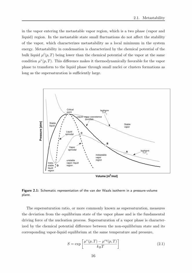
2.1. Metastability
in the vapor entering the metastable vapor region, which is a two phase (vapor and
liquid) region. In the metastable state small fluctuations do not affect the stability
of the vapor, which characterizes metastability as a local minimum in the system
energy. Metastability in condensation is characterized by the chemical potential of the
bulk liquid µl(p, T ) being lower than the chemical potential of the vapor at the same
condition µv(p, T ). This difference makes it thermodynamically favorable for the vapor
phase to transform to the liquid phase through small nuclei or clusters formations as
long as the supersaturation is sufficiently large.
Volume [m3/mol]
Pre
ss
ure
[a
tm]
Criticalpoint
Stablevapor
IsothermT<T
c
A
B
C
D
Liquid−vapor coexistence(binodal)
Vapor spinodal
Liquid spinodal
Stableliquid
meta−stableliquidregion
metastablevaporregionunstable
vapor−liquidregion
IsothermT=T
c
Figure 2.1: Schematic representation of the van der Waals isotherm in a pressure-volumeplane.
The supersaturation ratio, or more commonly known as supersaturation, measures
the deviation from the equilibrium state of the vapor phase and is the fundamental
driving force of the nucleation process. Supersaturation of a vapor phase is character-
ized by the chemical potential difference between the non-equilibrium state and its
corresponding vapor-liquid equilibrium at the same temperature and pressure,
S = exp
[µv(p, T )− µeq(p, T )
kBT
](2.1)
16

Chapter 2. Aspects of homogeneous nucleation
where kB is the Boltzmann constant, T is the thermodynamic temperature and µeq(p, T )
is the molecular chemical potential of the vapor-liquid equilibrium state at the same
pressure and temperature. In the case of an ideal gas the chemical potential difference
is defined as
µv − µeq = kBT lnpv
peq. (2.2)
Thus leading to S = pv/peq, which has the same functional form as the relative humidity.
In the case of a non-ideal vapor in mixture with a carrier gas, as in this research, the
change in chemical potential is determined by
µv − µeq = kBT lnfv
feq, (2.3)
where f represents the fugacity, which is an effective partial pressure that takes a
non-ideal gas behavior into account. The fugacity coefficient φ is defined as φ = f/yp
(with y the molar fraction of the vapor) and it gives the deviation from the ideal gas
(partial pressure). Thus, from eq. 2.2 it is clear that
S =fv
feq=
φ
φeq
y
yeq. (2.4)
Furthermore, if we assume that the neighboring molecules of the condensed molecules
are mostly carrier gas molecules in both equilibrium and the actual supersaturated
states, so that φ ≈ φeq, then S can be approximated as
S ≈ y
yeq=
ρ1
ρeq1(2.5)
with ρ1 the number density of the vapor. The second approximation is the form that
was used in the studies presented in the remaining chapters. As such, S characterizes
the degree of metastability of a system. When a vapor is under-saturated (S < 1) it
exhibits a distribution of unstable clusters that evaporate due to the higher chemical
potential of the liquid than the vapor. While in equilibrium, the cluster distribution
follows the Boltzmann distribution law.83 However, when the vapor is supersaturated
(S > 1), µl < µv, formation of liquid begins via molecules merging into clusters.
2.2 Thermodynamics of clusters
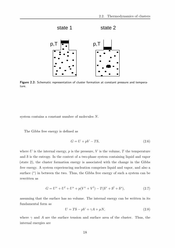
Let us consider the case of a closed system, isolated from its surroundings by a
piston, as shown in Fig. 2.2. In this figure the system is in transition from vapor
equilibrium (state 1) to a liquid cluster formation inside the vapor (state 2). The
17
2.2. Thermodynamics of clusters
Figure 2.2: Schematic representation of cluster formation at constant pressure and tempera-ture.
system contains a constant number of molecules N .
The Gibbs free energy is defined as
G = U + pV − TS, (2.6)
where U is the internal energy, p is the pressure, V is the volume, T the temperature
and S is the entropy. In the context of a two-phase system containing liquid and vapor
(state 2), the cluster formation energy is associated with the change in the Gibbs
free energy. A system experiencing nucleation comprises liquid and vapor, and also a
surface (s) in between the two. Thus, the Gibbs free energy of such a system can be
rewritten as
G = Uv + U l + Us + p(V v + V l)− T (Sv + Sl + Ss), (2.7)
assuming that the surface has no volume. The internal energy can be written in its
fundamental form as
U = TS− pV + γA+ µN, (2.8)
where γ and A are the surface tension and surface area of the cluster. Thus, the
internal energies are
18

Chapter 2. Aspects of homogeneous nucleation
Uv = TSv − pvV v + µvNv (2.9)
U l = TSl − plV l + µlN l (2.10)
Us = TSs + γA+ µsNs. (2.11)
For an initial homogeneous system (vapor) using Euler’s theorem for homogeneous
functions, the Gibbs free energy is given by
G0 = µ0N0, (2.12)
by assuming the equalities µ0 = µv, pv = p, taking into account conservation of
molecule numbers N0 = Nv +N l +N s, and incorporating eqs. 2.8-2.12 we obtain
∆G = G−G0 = N l(µl − µv) +Ns(µs − µv) + V l(pv − pl) + γA, (2.13)
The assumption that the core of the liquid cluster is in equilibrium with the interface,
in which case µs = µl applies, leads to
∆G = n∆µ− V l∆p+ γA, (2.14)
where n = N l+Ns is the total number of molecules in the cluster, ∆µ = µl(pl)−µv(pv)
and ∆p = pl − pv are the chemical potential and pressure differences between a cluster
and its surrounding vapor, respectively.
The interface between the liquid and vapor phase is modeled through capillarity
approximation, the fundamental assumption of the Classical Nucleation Theory (CNT)
developed by Volmer, Weber, Becker, Doring, and Zeldovich.11,139,158 Capillarity
approximation assumes that
• a liquid ”cluster” is spherical (vl = V l/n) and smooth as if it were a macroscopic
object with a well-defined radius, bulk liquid properties inside, and bulk vapor
properties outside;
• the thickness of the interface between the cluster and vapor is infinitely thin and
its energy is equal to the bulk phases at equilibrium
• the liquid is considered incompressible, µl − µeq = vl∆p.
19

2.2. Thermodynamics of clusters
Taking these assumptions into consideration, we arrive at
∆µ = (µl − µeq) + (µeq − µv). (2.15)
From eq. 2.1 and the incompressibility assumption above, we find that
∆µ = vl∆p− kBT lnS. (2.16)
Substitution in 2.14 yields that
∆G = −nkBT lnS + γA. (2.17)
The radius of a cluster with n molecules is given by
rn =
(3vl
4π
)n1/3 = r1n
1/3, (2.18)
where r1 is the radius of a single molecule. Therefore, the area of the cluster is
an = A = 4πr2n = 4πr2
1n2/3. The reduced free energy of the cluster formation is now
given by∆G
kBT= θn2/3 − n lnS, (2.19)
with the reduced surface tension
θ =a1γ
kBT, (2.20)
where the first term on the right-hand side of eq. 2.19 represents the contribution to
the interface created between the vapor and liquid and the second term represents the
bulk formation. From eq. 2.19, for a fixed T , ∆Gn can be plotted as a function of n
and S.
Fig. 2.3 shows the behavior of the free energy of under-saturated, saturated,
and supersaturated states. Whenever the system is (under)saturated S ≤ 1, ∆Gn
monotonously increases. However, if the system is supersaturated S > 1, ∆Gn increases
up to point n∗ and then decreases. In such cases, clusters smaller than n∗ are unstable
and tend to evaporate, while clusters that are larger than n∗ could become stable and
grow further. Thus, the profile of the free energy is a function of n, and the maximum
20

Chapter 2. Aspects of homogeneous nucleation
100
101
102
103
−50
0
50
100
150
200
250
300
n
∆ G
n [k
B T
]
S = 10
S = 6
S = 3
S = 1
S = 0.1
Figure 2.3: Free energy formation of cluster of n molecules at different supersaturations (S).
value of the function is reached when
n∗ =
(2θ
3 lnS
)3
, (2.21)
which represents the so-called critical cluster size and indicates the limit a cluster
needs to overcome in order to become a stable droplet. From this equation, the energy
barrier is established as∆G∗
kBT=
4
27
θ3
(lnS)2. (2.22)
2.3 Nucleation kinetics
An increase in size of an n-mer (cluster containing n molecules) is presumed to be
the result of collisions with other molecules and a reduction in size is presumed to
result from the loss of single molecules. In order to capture growth or reduction, CNT
uses the kinetic model of Szilard,31 which assumes that
• the change in size of a cluster occurs through impingement or loss of a single
molecule;
• the probability of a molecule colliding with a cluster and sticking is equal to
unity;
• no correlation is made between successive size change events.
21

2.3. Nucleation kinetics
bn+1ρn+1
ρnρn−1
bn
fn−1 fn
Figure 2.4: Schematic representation of the nucleation kinetics; fn is the forward rate, bn isthe backward rate, and ρn is the number density of an n-cluster.
Fig. 2.4 shows the schematic illustration of these assumptions in the kinetics of
nucleation. The illustration depicts fn as the forward (condensation) rate of one
molecule addition to an n-mer, where n becomes n+ 1, and depicts bn as the backward
(evaporation) rate, which refers to the loss of one molecule so that the n-mer becomes
an (n− 1)-mer. The non-equilibrium number density ρn change rate is described by
backward and forward losses on one hand, and increases from both the forward rate of
the previous step and the backward rate of the next step, on the other hand.
dρndt
= fn−1ρn−1(t) + bn+1ρn+1(t)− fnρn(t)− bnρn(t) (2.23)
The exchange rate between n-mers and (n+ 1)-mers is defined as
Jn(t) = fnρn(t)− bn+1ρn+1(t), (2.24)
so that the Becker-Doring11 kinetic equations becomes
dρndt
= Jn−1(t)− Jn(t). (2.25)
The formulation of the forward rate fn depends on the type of phase transition. For
the gas to liquid transition, the impingement rate j with a unit surface in the kinetic
theory of gases is j = p/√
2πmkBT . Therefore, the collision rate of the monomers with
the surface of an n-mer can be written as
fn = jan =
(kBT
2πm
)1/2
a1n2/3ρ1, (2.26)
in which m is the molecular mass of the vapor and ρ1 is the monomer number density.
The evaporation rate bn is not known a priori. To calculate this rate, CNT uses
the principle of detailed balance at the constrained equilibrium condition, called the
22

Chapter 2. Aspects of homogeneous nucleation
'kinetic theory of nucleation',72,71 where transition rates are equal in both directions,
Jn(t) = 0. At the constrained equilibrium, Jn = 0 holds for all n-mers, and their
distribution ρneq is time independent. Thus, from eq. 2.24 we find
bn+1 = feqnρeqnρeqn+1
. (2.27)
If a steady non-equilibrium state is assumed, where dρn/dt = 0 for all n, then all
the Jn rates can be replaced by a single steady-state nucleation rate, Js. describes the
number of nuclei (clusters) formed per unit volume and time. Substituting Jn = Js
and eq. 2.27 into eq. 2.24 we arrive at
Js = fnρn − feqnρeqnρeqn+1
ρn+1. (2.28)
We have seen that fn is proportional to ρ1, the monomer density, which is also
proportional to the partial pressure of the vapor (provided that the vapor contains
mainly monomers). This proportionality implies that fn/feqn = S. Dividing eq. 2.28
by fnρeqn S
n yields (note that Sn denotes S to the power n)
Jsfnρ
eqn Sn
=ρn
Snρeqn− ρn+1
Sn+1ρeqn+1
. (2.29)
Summation of this expression from n = 1 to N results in
Js
N∑n=1
(1
fnρeqn Sn
)= 1− ρN+1
SN+1ρeqN+1
. (2.30)
For sufficiently large N the last term on the right side can be neglected.64 By extending
the summation to infinity and replacing it with an integral, we can write the steady-state
nucleation rate as
Js =
[ ∞∫1
1
fnρeqn Sn
dn
]−1
, (2.31)
while considering n a continuous variable. To proceed with the integral calculation,
the Courtney distribution model25 is adopted for the equilibrium number density of
n-mers, given by
ρeqn Sn = ρeq1 exp(n lnS − n2/3θ) = ρeq1 exp
(− ∆G
kBT
). (2.32)
The exponent in this equation has its minimum close to the critical size n∗, meaning
23

2.3. Nucleation kinetics
that in the integral (eq. 2.31) the largest contribution is around the n∗ value. The
non-equilibrium formation energy can be thus written in a Taylor series form close to
n∗ as
∆G ' ∆G∗ − Z2πkBT (n− n∗)2, (2.33)
with Z being the Zeldovich factor
Z =
[− 1
2πkBT∆G′′(n∗)
]1/2
=1
3
(θ
π
)1/2
(n∗)−2/3, (2.34)
where the double prime denotes the second derivative. Substituting eqs. 2.32 and 2.33
into eq. 2.31 leads to
Js = fn∗ρeq1
∞∫1
[−Z2π(n− n∗)2]dn
−1
exp
(− ∆G∗
kBT
). (2.35)
If the lower limit in the integration is changed to −∞, a Gaussian type integral can
be recognized with a solution Z−1. By further incorporating eqs. 2.22, 2.26, and 2.34
the formulation of Js finally becomes
Js = ρ1ρeq1 v
l
(2γ
πm
)1/2
exp
[− 4
27
θ3
(lnS)2
]. (2.36)
This expression of the nucleation rate thus combines the thermodynamics and
kinetics of the molecular system. Even though CNT is able to capture the underlying
physics and provide a qualitative description of the nucleation phenomena,152 it
fails to provide a good quantitative description of water nucleation,16,18,138,58 or
nucleation of other substances,137 or nucleation in multicomponent systems.124,66
Another shortcoming of CNT is that it is unable to explain the vanishing nucleation
barrier at high supersaturations.123 Although various extensions14,42,41 and other
theoretical approaches64,68,29,121,65 have been developed, CNT is favored in practice
and remains a reference in nucleation studies. The CNT expression in eq. 2.36 (for
which ρ1ρeq1 = ρ2
1) is used for comparison with the simulation results in Chapters 3, 4,
and 5. The monomer density ρ1 can directly be obtained from molecular dynamics
simulations and the molecular liquid volume vl and surface tension γ is taken from
literature.
24

Chapter 2. Aspects of homogeneous nucleation
2.4 Molecular modeling
Computational molecular simulations constitute a powerful tool to describe the
nucleation process at its earliest stage. Molecular simulations trace molecules by using
detailed information of atomic positions, velocities and forces that allow understanding
of the microscopic origin of physical properties that cannot be accessed experimentally.
The use of computer simulations to investigate properties of condensed matter dates
back to the 1950’s when the first MC96 and MD simulations were performed.2 Both
Monte Carlo (MC) and Molecular Dynamics (MD) simulations are computational
techniques that essentially ”sample” ensembles. The main difference between MC
and MD is that MC simulations generate sequences of configurations stochastically,
while MD simulations generate configurations in a deterministic manner by computing
the time evolution of the system. Thus, the macroscopic properties of a system
calculated from molecular interactions in MC are averaged ensembles and in MD
they are time averages. These averages are equal according to the fundamentals
of molecular simulations (Ergodic hypotheses37). MC has been previously used to
study homogeneous nucleation94 by sampling random molecular configurations and
estimating free energies of formation of the small embryos. However, MC simulations
do not provide information about time evolution. On the other hand, MD simulates an
experiment and provides a complete description of the system structure and dynamics,
as it studies the temporal evolution of the coordinates and velocities of the given
macromolecular structure. As such, in this research MD simulations were used to study
homogeneous nucleation.
Statistical mechanics
Statistical mechanics is the field of study that relates the classical physics or
properties measured in a typical experiment with quantum physics by using statistical
methods, probability theory, and the microscopic physical laws. In the following,
the principles and available tools that provide the connection between the macro
and microstate of a system in a simulation are presented as groundwork prior to the
introduction of MD.
2.4.1 Ensembles
To completely characterize a system of one mole of a substance or around 1023
atoms, the three components of velocity and three components of the position of each
25

2.4. Molecular modeling
atom are needed. This characterization is currently impossible to handle computation-
ally. However, when describing the state of any system, the average thermodynamic
properties such as the pressure, volume, and temperature are typically considered. To
calculate these properties, statistical physics uses the principle that all possible states
appear with an equal probability, meaning that a given system can have a number
of configurational microstates that all have the same thermodynamic properties or
macrostate. Still, the system can only be in one state at a given time. As such, each
possible state appears the same number of times among the copies of the system.
The collection of all these possible states under the same macroscopic condition is
called an ensemble. Thus, statistical mechanics deals with ensembles rather than
individual systems. Fixing three macroscopic properties of a systems implies that the
ensemble will also have three fixed macroscopic properties. During time evolution of a
macroscopic system in a fixed macrostate, the microstate is supposed to pass through
all the possible states.
Depending on the interaction of the system with its surroundings, the thermodynamic
system can be classified as an isolated, closed or open system. Similarly, statistical
ensembles are also classified into three different categories.
Micro-canonical (NVE) ensemble
The microcanonical ensemble corresponds to an isolated system, in which neither
energy nor matter (mass) is exchanged with its surroundings. It is also called the NVE
ensemble, as each isolated system in the ensemble has a constant number or particles
(N), volume (V) and total energy (E), while all the other properties are allowed to
fluctuate. Here, it is assumed that constant energy refers to an energy level that lies
within E and E+δE, with δE → 0. The number of all possible system configurations
(quantum states) in the ensemble corresponding to energy E is denoted as Ω(E), also
called the micro-canonical partition function.92 The thermodynamic properties can
then be obtained by correlating the entropy of the system A (SA) with the number of
all possible states, Ω. From the statistical definition of entropy by Boltzmann, if an
experiment has N possible outcomes with equal probability, the entropy SA = kB log Ω,
where kB is the Boltzmann constant. As stated in the second law of thermodynamics,
the equilibrium corresponds to maximum entropy and implicitly to the maximum Ω.
26

Chapter 2. Aspects of homogeneous nucleation
Canonical (NVT) ensemble
The canonical ensemble corresponds to a closed system exchanging only energy (not
matter) with its surroundings. In this ensemble the controlled and fixed properties are
N, V and T. This ensemble is most commonly used in simulation studies of fluids with
known densities to predict properties such as pressure, transport properties, internal
energy, etc. Although the system is in thermal equilibrium with a heat bath, the energy
can vary from zero to infinity thereby, having an energy state Es for each microstate
s. The probability for the system to be in microstate s is eEs/kBT and the canonical
partition function is defined as
Z(N,V, T ) =∑s
e−Es/kBT (2.37)
The Helmholtz free energy of the system is related to the logarithm of the partition
function and is given by
A(N,V, T ) = −kBT lnZ(N,V, T ) (2.38)
All equilibrium thermodynamic properties can be deduced by taking derivatives
of the free energy with respect to its parameters. As such, the partition function of
an ensemble is the key parameter in statistical mechanics to computing most of the
thermodynamics state variables of a system.
Grand canonical ensemble
The grand canonical ensemble, also called the µV T ensemble, corresponds to an
open system where both energy and matter are exchanged with the surroundings. The
fixed properties here are V, T, and µ, i.e. the system is in thermal and chemical
equilibrium with a reservoir. This ensemble is the only one with a fluctuating number
of particles in the system, and it is mostly used in adsorption or chemical reaction
studies.
Isothermal-isobaric(NpT) ensemble
In the isothermal-isobaric (NpT) ensemble the amount of particles N, pressure p,
and temperature T are constrained. Although this ensemble does not correspond to a
typical thermodynamic system, it is widely implied in simulations as it enables the
prediction of thermophysical properties from constrained experimental conditions.
27
2.4. Molecular modeling
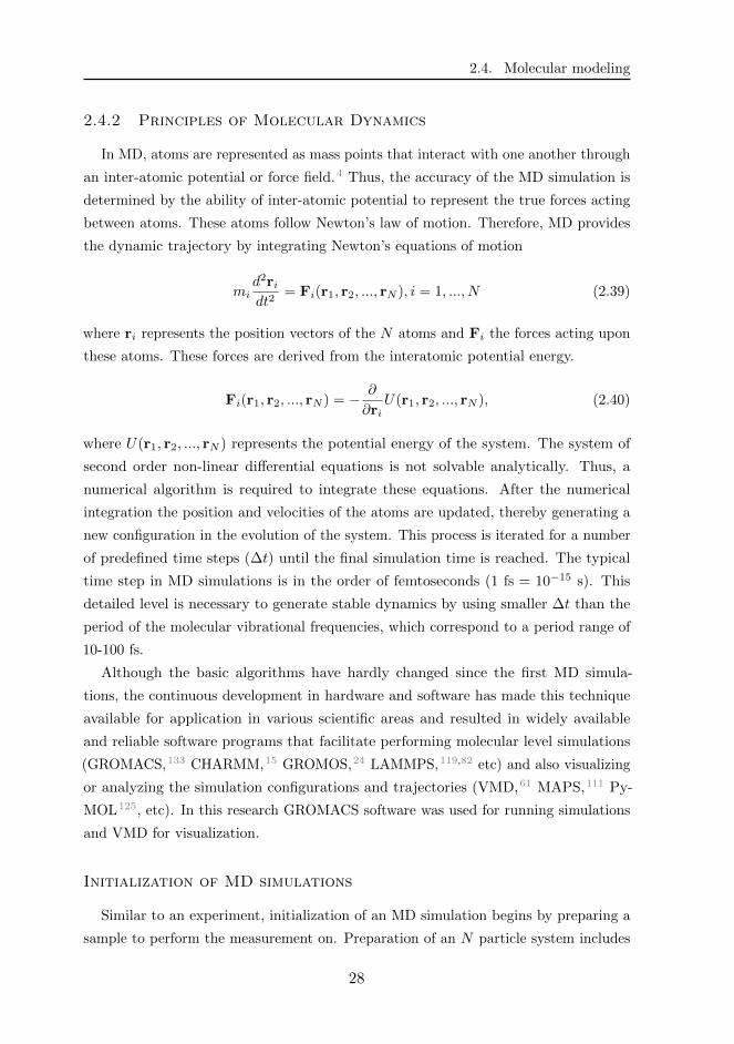
2.4.2 Principles of Molecular Dynamics
In MD, atoms are represented as mass points that interact with one another through
an inter-atomic potential or force field.4 Thus, the accuracy of the MD simulation is
determined by the ability of inter-atomic potential to represent the true forces acting
between atoms. These atoms follow Newton’s law of motion. Therefore, MD provides
the dynamic trajectory by integrating Newton’s equations of motion
mid2ridt2
= Fi(r1, r2, ..., rN ), i = 1, ..., N (2.39)
where ri represents the position vectors of the N atoms and Fi the forces acting upon
these atoms. These forces are derived from the interatomic potential energy.
Fi(r1, r2, ..., rN ) = − ∂
∂riU(r1, r2, ..., rN ), (2.40)
where U(r1, r2, ..., rN ) represents the potential energy of the system. The system of
second order non-linear differential equations is not solvable analytically. Thus, a
numerical algorithm is required to integrate these equations. After the numerical
integration the position and velocities of the atoms are updated, thereby generating a
new configuration in the evolution of the system. This process is iterated for a number
of predefined time steps (∆t) until the final simulation time is reached. The typical
time step in MD simulations is in the order of femtoseconds (1 fs = 10−15 s). This
detailed level is necessary to generate stable dynamics by using smaller ∆t than the
period of the molecular vibrational frequencies, which correspond to a period range of
10-100 fs.
Although the basic algorithms have hardly changed since the first MD simula-
tions, the continuous development in hardware and software has made this technique
available for application in various scientific areas and resulted in widely available
and reliable software programs that facilitate performing molecular level simulations
(GROMACS,133 CHARMM,15 GROMOS,24 LAMMPS,119,82 etc) and also visualizing
or analyzing the simulation configurations and trajectories (VMD,61 MAPS,111 Py-
MOL125, etc). In this research GROMACS software was used for running simulations
and VMD for visualization.
Initialization of MD simulations
Similar to an experiment, initialization of an MD simulation begins by preparing a
sample to perform the measurement on. Preparation of an N particle system includes
28

Chapter 2. Aspects of homogeneous nucleation
the creation of a starting configuration of the system to investigate. As such, the initial
positions and velocities of the N particles are required. In the case of crystal structures,
these positions are predefined in a crystallographic data file. For disordered systems,
such as those sampled in this work, the positions are randomly distributed and exclude
overlapping atoms. The velocity of each atom is randomly attributed according to
the Maxwell-Boltzmann distribution which corresponds to the set temperature of the
system. For statistical accuracy, independent starting configurations of a system are
commonly used, where the system is replicated and individual particles are assigned
different initial positions and velocities.
While the fraction of edge particles in the macroscopic system is negligible, this
is not the case in MD simulations. The system size and particle number ranges in
MD simulations are between nanometer to micrometer and thousands to millions of
particles, in which edge particles are proportional to a fraction of N−1/3. Due to this
high fraction of edge particles, the choice of boundary conditions (fixed, free or periodic)
cannot be assumed to have a negligible effect on the evaluation of the bulk properties
of the system. In this work, we study disordered systems that simulate bulk phases, for
which it is essential to avoid surface effects. Thus, periodic boundary conditions4 are
employed to mimic the immersion of the N particle system in an infinite bulk system
represented by identical replicas of the system.
The initial configuration of the system is not representative of the thermodynamic
system to be investigated. To further facilitate the system rapidly reaching thermody-
namic equilibrium the system needs to attain a local minimum of the potential energy.
This local minimum is ensured through an energy minimization simulation by using
the iterative steepest descent or conjugate gradient method.160
Running Equilibration or Production simulation
The following step after sample preparation is performed to connect the sample to
the measuring tool. In MD this is performed by running an equilibration simulation.
Now that the system is equilibrated and corresponds to a real thermodynamic system,
the actual measurement can be performed on the sample, which in MD corresponds
to the production simulation run. Running an equilibration or production simulation
essentially means solving the differential equation in eq. 2.39 using an NVE, NPT or
NVT ensemble until the thermodynamic properties fluctuate around their set condition
values.
To numerically solve eq. equation (2.39) in this research we use the so-called leap-frog
integrator.55 Leap-frog is a stable method that supports conservation of energy, has
29

2.4. Molecular modeling
higher stability than the more complex integrators, and requires lower memory to
implement. The atom coordinates, velocities and accelerations are updated in the
leapfrog method as follows
ri(t) = ri(t−∆t) + vit−∆t
2∆t, (2.41)
ai = F(ri(t))/mi, (2.42)
vit+∆t
2= vit−
∆t
2+ai(t)∆t, (2.43)
where vi = (d/dt)r is the velocity, ai = (d2/dt2)r is the acceleration, and mi is the
mass of atom i.
Truncation, short-range and long-range interactions
In MD, the computational effort required to evaluate the forces between all N atoms
of a system is proportional to N2. Hence, as the number of particles increases so
does the computation time. Thus, to reduce unnecessary computation effort in a large
system, periodic boundary conditions are used together with spherical truncation for
the computation of the particle interactions (potential). In the latter approach, only
the interactions separated by a distance smaller than rcut are considered
ULJtrunc(r) :=
ULJ(r) for r ≤ rcut
0 for r > rcut.(2.44)
The value of rcut should be smaller than half the length of the simulation box because
at larger values interactions between a particle and its own periodic image in the
neighboring replica box might be computed as a particle-particle interaction. Still, the
rcut should be large enough such that interactions beyond rcut become negligible. In
MD the total intermolecular potential is split into short-range and long-range forces.
Short-range interactions decay rapidly with distance. Thus, the spherical truncation
can be safely applied to the short-range interactions, typically represented by the
Lennard-Jones (LJ) potential:
ULJ = 4ε
[(σr
)12
−(σr
)6]. (2.45)
The parameter ε is the potential well depth, σ is the distance at which the potential
becomes zero, and r is the inter-atomic distance. In this research values of 99 and
30
Chapter 2. Aspects of homogeneous nucleation
40 A were used for truncation. Such rather large values of potential cutoffs were
essential to obtain reliable force calculations for non-equilibrium conditions in large
simulation boxes. The long-range interactions consist of electrostatic or Coulombic
interactions outside of the rcut and are infinite ranged. Hence, a simple truncation is
not applicable. To account for the long-range interactions, the effect of periodic images
must be considered. The most commonly used method to decompose the Coulombic
forces and evaluate long-range interactions is the so-called Ewald summation.30 In this
research we used a more efficient method derived from Ewald summation, the Particle
Mesh Ewald summation27 (PME). In this approach point charges are interpolated over
a mesh to obtain a discretized Poisson equation. This equation is solved using the
Fast Fourier Transform to obtain the electrostatic energy. In the PME approach, for
accuracy reasons, the total electrostatic energy is defined as Eel = Esr + Elr, where
the first element in the summation is the sum of the short-range potential in real space
and the second element is the summation in Fourier space of the long-range part of the
potential. In this research, the Fourier spacing was set at 0.12 nm and the short-range
electrostatic interactions were truncated at the same value as the LJ truncation.
Temperature and pressure control
In an NVE ensemble the total energy is kept constant, whereas the kinetic and the
potential energy contributions can fluctuate. If we take for example a system that
has not reached equilibrium, the system will experience temperature changes until it
achieves equilibrium. To rapidly reach equilibrium in MD simulations, temperature or
pressure control is applied by removing heat or stress from the system. This control is
available through a thermostat or a barostat. In this work, several thermostats and
barostats were used and are described below.
The instantaneous temperature of a system in MD is related to the kinetic energy,
Ek =
N∑i=1
p2i
2mi=kBT
2Ndf , (2.46)
where Ndf is the total number of degrees of freedom of the particles (in MD defined as
3N −Nc −Ncom, Nc is the number of constrains on the systems and Ncom = 3 the
center-of-mass removal) and pi is the momentum of atom i. As such, the temperature
can be controlled by rescaling the velocities of the atoms.
To maintain constant temperature the easiest algorithm to use is the (simple) velocity
scaling (VS). In this approach the velocities are scaled regularly by a factor λ =√T0/T ,
31

2.4. Molecular modeling
where T0 is the desired (thermostat) temperature and T is the instantaneous current
temperature of the system.
A similar approach, but which scales with each time step, is the Berendsen thermostat
approach,12 in which the system temperature decays exponentially to the desired
temperature with
∆T =δt
τ(T0 − T ), (2.47)
where δt is the simulation time step and τ is the time constant. The time constant
determines how quickly the desired temperature will be reached. Both Berendsen
and VS algorithms allow rapid achievement of the desired temperature, and are thus
recommended for the equilibration phase of a system (provided that the time constant
is small enough). However, both thermostats suppress natural temperature fluctuation
and thus do not sample the dynamics of a true NVT ensemble.101 In this work, a
Berendsen thermostat was used for system equilibration with a typical MD time
constant of 0.1 ps. The VS was used with a smaller τ of 0.025 ps to rapidly decrease
the temperature to the desired nucleation temperature and to thermostat the carrier
gas in production runs.
A more physically realistic thermostat is the Nose-Hoover107 (NH) thermostat. In the
NH thermostat the imaginary heat bath becomes an integral part of the system, where
large but realistic oscillations around the desired value adjust the system temperature.
The period of these oscillations is defined as τ2NH = Q/(NdfkBT0), where Q and
T0 are the strength of the coupling to the heat bath and the reference temperature
of the heat bath, respectively. This slow damping oscillatory relaxation algorithm
causes poor temperature control and requires longer computation times to attain
equilibrium. However, the NH thermostat is recommended for production runs where
system dynamics is relevant because it samples the true canonical ensemble. Thus, the
NH thermostat was also employed in production runs of our research.
The instantaneous pressure tensor in an MD simulation is directly related to the
virial tensor by
P =2
V
Ek +1
2
N∑i<j
rijFij
, (2.48)
where rij and Fij is the inter-atomic distance and force, respectively. Thus, to control
the pressure, the volume of the simulation box is scaled. Further, the pressure is
derived from the trace of the pressure tensor: P = Tr(P)/3.
Similar to its thermostat counterpart the Berendsen barostat decays exponentially
32

Chapter 2. Aspects of homogeneous nucleation
to reach the desired pressure by
∆P =δt
τP(P0 − P ). (2.49)
where P0 is the set desired pressure and τP the coupling constant.
The Parrinello-Rahman barostat112 represents the true NPT ensemble and follows
the same principle as the NH thermostat. Compared to the Berendsen barostat, the
Parrinello-Rahman barostat allows for shape deformations of the simulation box in
addition to size deformation. The inverse matrix parameter determines the strength of
the coupling by
W−1ij =
4π2βij3τ2PL
, (2.50)
where β is the isothermal compressibility of the system. The Parrinello-Rahman barostat
coupling is recommended only for systems that have already achieved equilibrium,
because in the case of system far from equilibrium, coupling may result in large
dampening oscillations of the box size. In the current research τP was set to 0.1 ps and
the earlier mentioned barostats were employed in the equilibration phase after running
an NVT ensemble.
Molecular models
At the molecular level the underlying model that describes the behavior of a system
is called the force field. A force field (FF) is a mathematical expression that defines
the inter-atomic potential energy by using a set of parameters. Depending on the
development procedure and (experimental or theoretical) input data for the optimization
of these parameters,87,129 various FF have been developed. A typical functional form
of a FF is composed of bonded and non-bonded terms as follows
Etotal = Ebond + Eangle + Edihedral + Eelectrostatic + EvdW . (2.51)
The first three terms on the right-hand side represent the intramolecular or bonded
contributions, in which the bond stretching has a harmonic form,
Ebond =1
2kb(l − l0)2. (2.52)
33

2.4. Molecular modeling
In the same way, angle bending is represented as
Eangle =1
2kΘ(Θ−Θ0)2, (2.53)
while for the dihedral torsional energy,
Edihedral =
3∑n=1
kΦ,n(1 + cos(nΦ− Φn,0)), (2.54)
the values of the bond strengths kb, kΘ, kΦ,n and the parameters l0, Θ0 and Φn,0 are
given by the force field.
The last two terms in eq. 2.51 represent the non-bonded or intermolecular interactions,
in which the functional form of the electrostatic energy is
Eelectrostatic =1
4πε0
∑i<j
qiqjrij
, (2.55)
where qi, qj represent the atomic charges, rij the inter-atomic distance, ε0 is the vacuum
permittivity. The functional form for the van der Waals interaction in the current
research was represented by the LJ potential (see eq. 2.45).
In this research, nucleation was simulated in systems containing water or carbon
dioxide as condensing phases and argon, helium or methane as thermostatting gases. For
each particular component, one or two models were chosen to represent the interatomic
forces.
In Chapter 3 the TIP4P63 and TIP4P/20051 models were used to represent water
and LJ was used to model the monoatomic argon. It has been shown that the
TIP4P model qualitatively reproduces the phase diagram, whereas the improved model
correctly predicts the phase diagram of water7,135 and a variety of physico-chemical
properties118,43. In this work the two different water models were used to analyze the
re-parametrization effect of the TIP4P model on the nucleation process.
The topologies of TIP4P and TIP4P/2005 model are very similar and are defined
as rigid molecules that have 4 interaction sites. Three of these sites coincide with the
oxygen and hydrogen atom positions. The other site is a massless dummy M site,
coplanar with the O and H sites and located at the bisector of the H-O-H angle. The
distance between O-H and the angle between H-O-H are fixed to the experimental
values, 0.9572 A and 104.52°, respectively. The only difference in topology is the O-M
distance, which is 0.15 A for the TIP4P and 0.1546 A for the TIP4P/2005 model.
Regarding the interactions, there is a single LJ contribution at the oxygen site and
34

Chapter 2. Aspects of homogeneous nucleation
electrostatic charges at the hydrogens and the M site, where qH = −qM/2. The
parameter values of the water and argon potential models are given in Table 3.1.
In Chapter 4 helium and methane are used as carrier gases. Both carriers were
represented as monoatomic gases and LJ potential was employed with the parameter
values shown in Chapter 3, Table 4.1.
In Chapter 5 nucleation of carbon dioxide in methane are discussed. The linear
carbon dioxide molecule was modeled using the elementary physical model 2 (EPM2),50
which has two rigid bonds and a flexible bond angle. To implement this model a virtual
site topology of the EPM2 model was used, in which two massive atoms have each
half the mass of the CO2 molecule and the virtual sites are at the position of the
carbon and oxygen atoms. Instead of using bonds, in the virtual site topology the
distance between the mass centers is fixed and the position of the mass centers is used
to reconstruct the positions of the virtual sites. The structure of the molecule and
potential parameters can be found in Figure 5.1.
2.4.3 Properties derived from molecular dynamics simulation
Thermodynamic properties
As discussed in the previous subsection, thermodynamic properties such as tem-
perature and pressure can be computed from molecular dynamics simulations using
eqs. 2.48 and 2.50, respectively. From these equations, the values of the instantaneous
temperature and pressure are obtained at each time step. As such, the thermodynamic
properties are estimated from time averages over the phase-space trajectory or the
statistical ensemble average.
Structural properties
The radial distribution function (RDF) or the pair correlation function, g(r), provides
information on the system’s local atomic structure by showing how density varies as
a function of distance r away from a reference. This is done by measuring the ratio
between the number density of atoms on a spherical shell of thickness δr at distance r
from an atom and the average number density of atoms. The general expression for
g(r) in a N particle system is defined as
g(n)(r1, . . . , rn) =V nN !
Nn(N − n)!
1
ZN
∫· · ·∫e−βUndrn+1 . . . drN (2.56)
where UN is the total potential energy of the system, V n is the volume of n-particles
35

2.4. Molecular modeling
system (n < N) and ZN =∫· · ·∫e−βUndr1 . . . drN , the so-called configurational
integral.22 In practice, the second-order correlation function g(2)(r1, r2) ≡ g(r) is of
high relevance in MD as it can be validated with experimentally determined g(r)
through X-ray diffraction77,40,145 or neutron diffraction measurements.134 The RDF
between particles of type a and type b can be calculated by
4πr2gab(r) =1
NaρB
Na∑i=1
Nb∑j=1
〈δ(|ri − rj | − r)〉 (2.57)
where Na and Nb is the number of a and b type atoms, respectively; ρB is the average
density of b type atoms over all spheres around atoms a, and δ is the shell thickness
relative to the distance between atom i and j, with 〈·〉 representing the ensemble
average. As such, gab(r) effectively counts the average number of b neighbors in a shell
at distance r around an a particle and represents it as a local density.
0 0.2 0.4 0.6 0.8 1 1.20
0.5
1
1.5
2
2.5
3
r
g OO
(r)
Figure 2.5: Radial distribution function determined from a 300 ps NVT simulation of bulkliquid water of 5000 molecules at a temperature of 350 K and a density of 971.3 mg/cm3.
In the case of a homogeneous system with uniform distribution of particles (bulk),
g(r) is normalized such that limr→∞ g(r) = 1. This behavior can be observed in Fig. 2.5,
in which an example of a radial distribution function for liquid water between oxygen
atoms is shown. The first peak in the RDF corresponds to the first coordination sphere.
The second peak is the attraction to particles in the first peak. In the same manner,
the third peak is the attraction to particles from the second peak. The magnitude
36

Chapter 2. Aspects of homogeneous nucleation
of these peaks diminishes, reflecting vanishing attractions as r becomes larger, while
the wells are due to the excluded volume of particles occupying the previous peak. At
large values of r, the distribution within the sphere becomes equal to the average bulk
density, and thus the RDF converges to 1. In the case of a liquid cluster in vacuum,
the profile of the RDF will decrease as r approaches the margins of the cluster until it
converges to 0.
In Chapter 5 the radial distribution is used to validate the virtual site topology
(built to reproduce the EPM2 model) against literature data, and to verify the liquid
structure of large carbon dioxide clusters obtained from our nucleation simulations.
Self-diffusion coefficient
Diffusion is a process caused by thermal motion of particles in a fluid. The law that
describes diffusion at macroscopic level is known as Fick's law, which relates the flux
of diffusing particles, j, to the concentration gradient, ∇c, by j = −D∇c, where D is
the diffusion coefficient.
In an MD simulation the trajectories of all atoms in an N particle system are
followed. As such, the phase space trajectory obtained from the ensemble facilitates
the computation of the diffusion coefficient. Einstein is one of such methods,44,78,52
which measures the mean displacement of the atoms from their initial positions to their
positions at time t
u2(t) =1
N
∑i
|ri(t)− ri(0)|2, (2.58)
where ri(0) is the initial position of atom i and ri(t) is the position of atom i at
time t. Self-diffusion is the diffusion of the constituent particles of a fluid among the
other identical particles. Furthermore, to determine the self-diffusion coefficient at
microscopic level, the Einstein relation93 can be used
D = limt→∞
u2(t)
6t, (2.59)
In Chapter 4 self-diffusivity derived from Einstein’s relation is used to validate the
employed helium, argon, and methane molecular models. It is known that Einstein’s
relation results in underestimation of diffusivity due to discontinuity of the particle
position when crossing the periodic boundary. However, in large sized systems of 1000
molecules this effect reduces.102 In our research the system was comprised of 5000
molecules, and as such this effect was strongly reduced.
37

2.4. Molecular modeling
38

3Nucleation of TIP4P and TIP4P/2005 water
model∗
3.1 Introduction
Understanding condensation phenomena is of great interest in environmental sci-
ences,120,13 biomedical studies8,106 and technological processes. A rich field of appli-
cations of condensation in multi-component gases is associated with the natural gas
industry. Liquefaction of natural gas involves several pre-treatment steps to remove
low concentration contaminants from natural gas such as water, carbon dioxide, ethane
and butane. These impurities should be removed to prevent blockages in pipeline
systems and heat exchangers and prevent crystal deposition at cryogenic conditions
on the process equipment during the actual liquefaction process. We are interested
in evaluating the natural gas pre-processing during cool down with very limited or
non-additional gas treatment, by investigating phase transitions for multi-component
gas mixtures.
Nucleation (the process by which embryos of the new phase are formed from the
∗The content of this chapter was previously published in the Journal of Chemical Physics.The original citation is as follows: Dumitrescu, L.R., Smeulders, D.M.J., Dam, J.A.M, andGaastra-Nedea, S.V., Homogeneous nucleation of water in argon. Nucleation rate computationfrom molecular simulations of TIP4P and TIP4P/2005 water model, The Journal of ChemicalPhysics, 146, 084309 (2017).
39

3.1. Introduction
parent phase) is the first step in the condensation process, followed by droplet growth
and possibly crystallization at low enough temperatures.113,81 The nucleation process
is called homogeneous when the presence of dust particles and foreign bodies can be
excluded and droplets are formed solely because the free energy associated with the
supersaturated vapor is large enough to overcome the excess free energy associated
with the embryo’s surface. The number of stable droplets formed per unit time and
volume (the so-called nucleation rate) is the key parameter in quantifying nucleation
processes and thus essential for understanding and controlling natural gas liquefaction.
In gas mixtures, the non-condensing phase or phases act as a heat reservoir to keep
the nucleating phase at isothermal conditions and the embryos are non-spherical.
Over the past years homogeneous nucleation processes have been studied both experi-
mentally51 and theoretically.32,70 However, no theoretical prediction model successfully
describes quantitatively nucleation of all substances under various conditions. The
most widely used theoretical model to understand nucleation is the Classical Nucleation
Theory (CNT). CNT was developed by Becker & Doring 11 , and Frenkel 38 (based on the
nucleation kinetic theory earlier established by Volmer & Weber 139 , and Farkas 31) and
later reformulated by Zel’dovich 158 . The theory assumes equilibrium properties for the
small embryos whereas nucleation process is obviously a non-equilibrium phenomenon.
Computer simulations, like molecular Monte Carlo (MC) and Molecular dynamics
(MD), have proved to be helpful tools to gain insight into systems behavior at molecular
level. Existing MC simulations for homogeneous nucleation94 sample random molecular
configurations and estimate free energies of formation of the small embryos. These are
then applied to a steady-state kinetic model for the nucleation rate. As such, MC can
not be used to study the real time evolution of the system. On the other hand, MD is
a promising technique to obtain a complete description of the dynamical properties
and it can be used to track the time evolution of the non-equilibrium dynamics.
Previously, an overview of nucleation of Argon using MD simulations was presented
by Kalikmanov et al. 67 showing that CNT results for the nucleation rates deviate by
approximately 3-5 orders of magnitude from MD simulations and by up to 26 orders
from the experiments.33
Yasuoka & Matsumoto 156 have studied water nucleation using the TIP4P model
in a carrier gas (Argon) and later extended the work to larger systems using SPC/E
water.90 In the former paper they reported on distribution of clusters, the critical
nucleus and fusion of clusters, but they did not report on the molecular composition
evolution of an individual cluster or the effect of the chosen water model on the results.
Molecular composition might explain the cluster stability dependence on the system
40

Chapter 3. Nucleation of TIP4P and TIP4P/2005 water model
configuration during the nucleation phase. Moreover, as nucleation is a stochastic
process, many independent MD simulations should be considered in order to improve
the accuracy of the nucleation rates. For water nucleation in a carrier gas, Yasuoka &
Matsumoto 156 considered two independent runs when determining the rates.
Due to stochastic behavior, scattered rates can be registered for different starting
configurations of the system. Investigation of the deviations of these rates together
with cluster stability and dynamics is important in order to understand in depth the
nucleation process.
Using different molecular models can lead to different results in the nucleation
behavior depending on how accurately the force field (FF) reproduces the thermo-
dynamic conditions of phase transitions. Yasuoka & Matsumoto 156 used the TIP4P
water model to simulate nucleation of water. It is still an open subject to asses and
compare different water models and their effect on the embryonic clusters undergoing
the nucleation process.
The surface tension values depend on the FF of the molecular model in use.91,3,131,157,62
In the study of Yasuoka & Matsumoto 156 , the predicted TIP4P surface tension is
smaller than the experimental and other literature values for water surface tension.
This could account for the CNT nucleation rate being almost two orders of magnitude
different from the simulation outcome. Using state-of-art surface tension values136 for
the same TIP4P water model, one can investigate the effect of surface tension on the
CNT prediction.
In this work we focus on understanding the stability of clusters and improving the
nucleation rates accuracy for mixtures that are used in gas pre-treatment. We gain
an understanding of the system dynamics by looking at distribution of the clusters
at different moments in time. We monitor the evolution of the individual molecules
forming a TIP4P water cluster from small, medium to large sizes. We analyze the
effect of the improved TIP4P/2005 water model. An error analysis is extracted from
six independent configuration runs to obtain the accurate nucleation rate. We compare
successfully our nucleation rate results with Yasuoka & Matsumoto 156 , the CNT
prediction and Hale’s theoretical scaled model prediction.46
3.2 Theory and Modeling
3.2.1 Classical Nucleation theory
The theory of homogeneous nucleation from vapor to liquid assumes microscopic
clusters to be macroscopic objects with well-defined bulk phase properties and surface
41

3.2. Theory and Modeling
free energy relative to the background vapor. The CNT free energy of cluster formation
is given by:
∆G = 4πr2γ − (4/3)πr3ρnl kBT lnS (3.1)
in which the first term is the positive contribution of the surface tension γ (surface-
free-energy per unit area) of the interface between liquid and vapor, and the second
term is the decrease in the free energy due to the bulk liquid formation. Starting from
the premise that we are in an ideal-vapor environment and the liquid is incompressible,
the pressure difference becomes ρnl kBT lnS, where ρnl is the liquid number density
of the cluster, kB the Boltzmann constant, T the system temperature and S the
supersaturation ratio. Supersaturation is the driving force of the nucleation processes
and it is defined as ρn/ρnsat, with ρn being the number density of the vapor and ρnsat
of the saturated vapor. The free energy difference reaches its maximum ∆G∗ when
the cluster of size n (number of molecules per cluster) attains the critical value n∗.
Deriving from expression (3.1), the size of the critical cluster can be written as
n∗ =32π
3
γ3
(kBT lnS)3(ρnl )2, (3.2)
and
∆G∗ =16π
3
γ3
(kBT lnSρnl )2, (3.3)
where n is obtained from n = ρnl V , and V is the spherical volume of the cluster.
CNT states that the nucleation rate, JCNT defined as the formation rate of the
clusters (of any size) per unit volume follows the expression: JCNT = K exp(−∆G∗
kBT),
where the kinetic prefactor K is defined as K = ρnZrf . The Zeldovich factor and the
forward rate are
Z =1
3
(θ
π
)1/2
(n∗)−2/3 (3.4)
rf = a0n2/3
√kBT
2πmρn, (3.5)
respectively, where m is the molecular mass and θ = γa0/(kBT ), with a0 as ”molecular
surface area”. Thus the classical expression of the nucleation rate becomes:
JCNT = (ρnl )−1
√2γ
πm(ρn)2 exp
(−∆G∗
kBT
).64 (3.6)
42

Chapter 3. Nucleation of TIP4P and TIP4P/2005 water model
3.2.2 Molecular Dynamics
MD is a computational technique which can be used to model and analyze dynamic
events in non-equilibrium states. With the help of MD we can predict macroscopic
thermodynamic properties of physical systems based on the time dependent dynamics
of many particle systems.
MD simulations generate trajectories of particles by means of direct numerical inte-
gration of Newton’s equations of motion. It is generally assumed that particles (atoms
or molecules) interact via effective atom-atom (or atom-molecule) pair potentials.39
For the Argon atoms we use the widely adopted Lennard-Jones (LJ) potential formula:
ULJ = 4ε
[(σr
)12
−(σr
)6]. (3.7)
where ε is the depth of the potential well, σ is the separation at which the potential is
zero and r is the interatomic separation. Water being a polyatomic polar molecule, more
interactions are considered including both the van der Waals and the ionic interactions.
Thus, the total non-bonded intermolecular potential becomes:
Uinter =∑a,b<a
4εOO
[(σOOrab
)12
−(σOOrab
)6]
+1
4πε0
∑i,j<i
qiqjrij
. (3.8)
The first term is the LJ (short-range) interaction between oxygen atoms, where εOO
is the interaction strength and σOO the length scale between the atom pairs separated
by a distance rab. The second term is the Coulombic (long-range) interactions between
the pairs of charged sites of the water molecules, where qi, qj represent their partial
charges and rij the distance between them; ε0 is the vacuum permittivity.
MD uses ensembles to simulate or compare properties of the system with a real
experiment. An ensemble is the statistical description of a macroscopic system which
uses a collection of large number of microstate states of the system under the same
macroscopic thermodynamic conditions. Our simulations generate NVE, NPT and
NVT ensembles.4
Periodic boundary conditions and minimum image convention are used for the
bulk phase (no free surfaces) MD simulations.4 A cutoff distance rcut, is used for the
LJ potential and the Particle mesh Ewald (PME)27 summation is implemented for
the Coulombic interactions. This method divides the interactions into short-ranged
components calculated in the real space, and the long-ranged components evaluated
using Fast Fourier transform.
To achieve constant temperature and pressure we adopt several methods. The
43

3.3. Molecular systems and simulations
Table 3.1: Intermolecular force field parameters for Argon and water molecular models.
Atom/Molecule ε/k (K) σ (A) qH (e)
Ar 119.8 3.405 -TIP4P53 78.0 3.154 +0.520TIP4P/20051 93.2 3.1589 +0.5564
Nose-Hoover107 thermostat is used to couple the system to an imaginary heat bath,
where large, but realistic oscillations adjust the system temperature. The period of
these oscillations is defined as τ2NH = Q/(NdfkBT0), where Q, Ndf and T0 are the
strength of the coupling to the heat bath, the total number of degrees of freedom of
the particles and the reference temperature of the heat bath, respectively. Due to its
slow damping oscillatory relaxation approach, the algorithm is more time consuming
during equilibration of the system at a given temperature.
For equilibration, we use the Berendsen thermostat12 because of the temperature
exponential relaxation towards the desired value. The velocities are scaled at each
time step, such that the change in temperature is proportional to the temperature
difference between the system and the heat bath: ∆T = δt/τ × (T0 − T ), where δt is
the simulation time step, T is the current instantaneous temperature of the system
and τ is the relaxation time. A faster method to bring the simulated system to the
desired temperature is the simple velocity rescaling.
Subsequent to temperature adjustment, pressure control in our simulation is achieved
by adjusting the volume of the simulation box via the Parrinello-Rahman barostat.112
Since the system has already reached equilibrium, the deformations of our simulation
box are negligible and account for a maximum of 2.7 % of its volume.
3.3 Molecular systems and simulations
We consider two different water models in our study: TIP4P and TIP4P/2005.
In order to study cluster dynamics and obtain a high statistical accuracy of water
nucleation processes, we construct six simulation boxes for each model with different
initial configurations of the same macroscopic system. Previous studies146,149 have
shown that simulation boxes containing more than 200 molecules provide reliable
statistics on cluster formation. Our simulation boxes consist each of 5000 water
molecules and 5000 Argon atoms. Argon is used as a heat bath and water is the
condensing phase. All simulation boxes are cubically shaped with a length of 28 nm,
chosen such as to reach the system equilibrium (mass) density ρ = 21.9× 10⁻³ g/cm3.
44

Chapter 3. Nucleation of TIP4P and TIP4P/2005 water model
Initial coordinates
Energy minimization
Equilibration dynamics(NVT)
1
Equilibration dynamics(NPT & NVE)2&3
is Temp.and
Press.reached?
Quench (NVT)4
Production phase (NVT)5
yes
no
(a)
−400 −200 0 200 400 600 800 1000 1200
−10
−5
0
5
10
15
20
25
Kinetic
Potential
1 2 3 54
Time [ps]
Pote
ntial and K
inetic E
nerg
y p
er
wate
r m
ole
cule
[kJ/m
ol/m
ole
c]
(b)
Figure 3.1: (a) Flowchart of the MD steps triggering nucleation. (b) Time evolution of thepotential and kinetic energy of water per molecule during the corresponding numbered steps inthe adjacent flowchart.
The initial average thermodynamic properties (T = 1000 K, p = 63 bar and
ρ = 21.9 × 10⁻³ g/cm3) agree with the GERG 200479 equation of state predictions
where the NIST REFPROP program84 was used.
Molecular computations are performed using periodic boundary conditions with
minimum image convention and leap-frog algorithm for the integration of Newton’s
equations of motion. The FF parameters for Argon, TIP4P and TIP4P/2005 models are
given in Table 3.1. The Lorentz-Berthelot combining rules are used for the interactions
between Argon and water. The molecular trajectories are generated using a time step of
δt = 0.5 fs. The process is carried out as follows (see Figures 3.1a and 3.1b). During the
equilibration steps 1 and 2 the vapor is kept at constant (averaged) temperature of 1000
K using the Berendsen thermostat with a relaxation time of τ = 0.1 ps. Furthermore,
the pressure is stabilized in step 2 using the Parrinello-Rahman barostat with the same
τ = 0.1 ps for the time constant. Next, a 200 ps NVE simulation (step 3) is performed
to provide a homogeneous starting configuration of the unperturbed system. The LJ
and the short-range Coulombic interactions are truncated both at rcut = 99 A.
Next, we trigger the nucleation process by quenching the system (step 4) into the
45
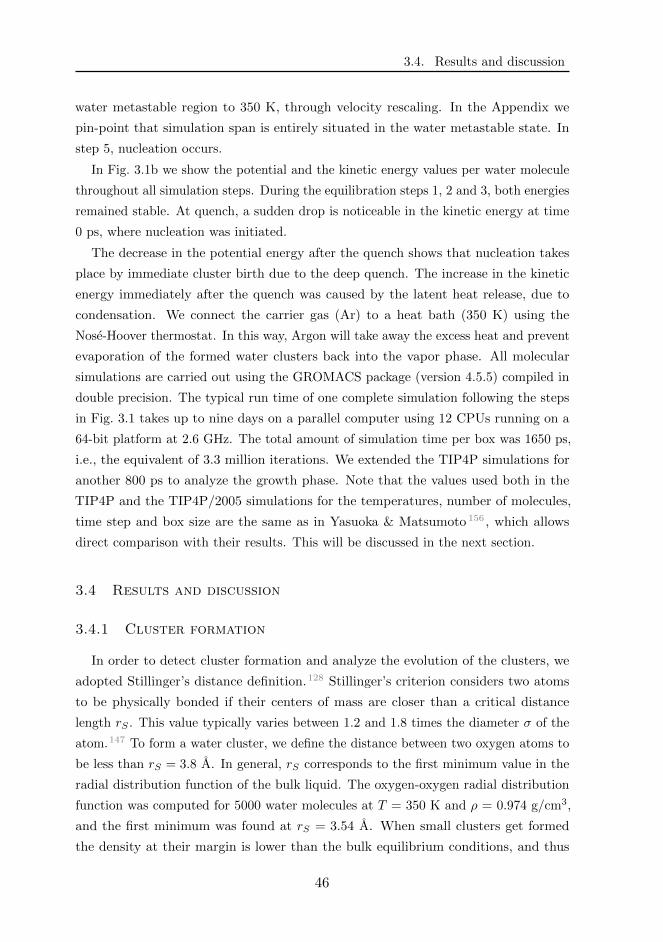
3.4. Results and discussion
water metastable region to 350 K, through velocity rescaling. In the Appendix we
pin-point that simulation span is entirely situated in the water metastable state. In
step 5, nucleation occurs.
In Fig. 3.1b we show the potential and the kinetic energy values per water molecule
throughout all simulation steps. During the equilibration steps 1, 2 and 3, both energies
remained stable. At quench, a sudden drop is noticeable in the kinetic energy at time
0 ps, where nucleation was initiated.
The decrease in the potential energy after the quench shows that nucleation takes
place by immediate cluster birth due to the deep quench. The increase in the kinetic
energy immediately after the quench was caused by the latent heat release, due to
condensation. We connect the carrier gas (Ar) to a heat bath (350 K) using the
Nose-Hoover thermostat. In this way, Argon will take away the excess heat and prevent
evaporation of the formed water clusters back into the vapor phase. All molecular
simulations are carried out using the GROMACS package (version 4.5.5) compiled in
double precision. The typical run time of one complete simulation following the steps
in Fig. 3.1 takes up to nine days on a parallel computer using 12 CPUs running on a
64-bit platform at 2.6 GHz. The total amount of simulation time per box was 1650 ps,
i.e., the equivalent of 3.3 million iterations. We extended the TIP4P simulations for
another 800 ps to analyze the growth phase. Note that the values used both in the
TIP4P and the TIP4P/2005 simulations for the temperatures, number of molecules,
time step and box size are the same as in Yasuoka & Matsumoto 156 , which allows
direct comparison with their results. This will be discussed in the next section.
3.4 Results and discussion
3.4.1 Cluster formation
In order to detect cluster formation and analyze the evolution of the clusters, we
adopted Stillinger’s distance definition.128 Stillinger’s criterion considers two atoms
to be physically bonded if their centers of mass are closer than a critical distance
length rS . This value typically varies between 1.2 and 1.8 times the diameter σ of the
atom.147 To form a water cluster, we define the distance between two oxygen atoms to
be less than rS = 3.8 A. In general, rS corresponds to the first minimum value in the
radial distribution function of the bulk liquid. The oxygen-oxygen radial distribution
function was computed for 5000 water molecules at T = 350 K and ρ = 0.974 g/cm3,
and the first minimum was found at rS = 3.54 A. When small clusters get formed
the density at their margin is lower than the bulk equilibrium conditions, and thus
46

Chapter 3. Nucleation of TIP4P and TIP4P/2005 water model
we consider a larger bond of rS = 3.8 A. Other definitions to define a liquid cluster
exist.126 In the study of Yasuoka & Matsumoto 156 , a cluster is defined by the potential
energy between two water molecules being smaller than −10 kJ/mol. Consequences of
the cluster definition are discussed in the forthcoming.
Number of water molecules in cluster [−]
Num
ber
of clu
ste
rs [−
]
10 20 30 60 100 200
0
1
2
3
t = 600 ps
10 20 30 60 100 200
0
1
2
3
t = 820 ps
10 20 30 60 100 200
0
1
2
3
t = 1240 ps
Snapshot (a)
Snapshot (c)
Snapshot (b)
a’
Figure 3.2: Cluster size distribution. Clusters having less than 10 water molecules are notshown. At t = 600 ps there is cluster (a’) and snapshots correspond to Figures 3.3a to 3.3c.
Using the Stillinger distance definition, in Fig. 3.2 a typical distribution of water
clusters at three different times is shown. In the top figure, at 600 ps after the quench,
small clusters with n ≤ 20 molecules dominate the cell, indicating that nucleation
has barely started. Yet, larger clusters having more than 20 water molecules were
already formed at this stage. At 820 ps the number of large clusters (between 20 and
50 molecules) is comparable with those at 600 ps, whereas few clusters grew larger
than 50 molecules. At 1240 ps, large clusters gathered more than 100 molecules. The
47
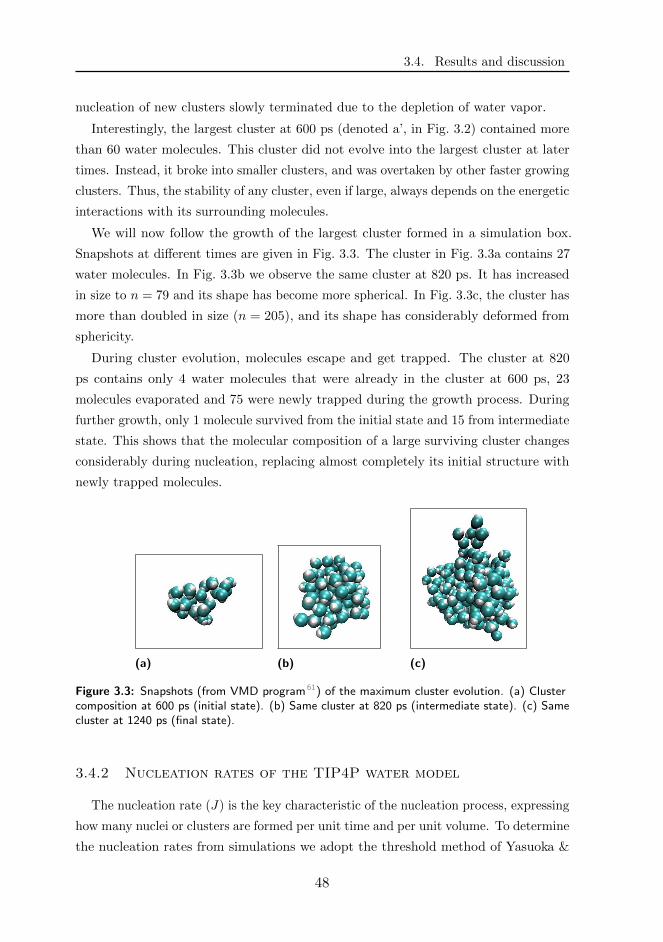
3.4. Results and discussion
nucleation of new clusters slowly terminated due to the depletion of water vapor.
Interestingly, the largest cluster at 600 ps (denoted a’, in Fig. 3.2) contained more
than 60 water molecules. This cluster did not evolve into the largest cluster at later
times. Instead, it broke into smaller clusters, and was overtaken by other faster growing
clusters. Thus, the stability of any cluster, even if large, always depends on the energetic
interactions with its surrounding molecules.
We will now follow the growth of the largest cluster formed in a simulation box.
Snapshots at different times are given in Fig. 3.3. The cluster in Fig. 3.3a contains 27
water molecules. In Fig. 3.3b we observe the same cluster at 820 ps. It has increased
in size to n = 79 and its shape has become more spherical. In Fig. 3.3c, the cluster has
more than doubled in size (n = 205), and its shape has considerably deformed from
sphericity.
During cluster evolution, molecules escape and get trapped. The cluster at 820
ps contains only 4 water molecules that were already in the cluster at 600 ps, 23
molecules evaporated and 75 were newly trapped during the growth process. During
further growth, only 1 molecule survived from the initial state and 15 from intermediate
state. This shows that the molecular composition of a large surviving cluster changes
considerably during nucleation, replacing almost completely its initial structure with
newly trapped molecules.
(a) (b) (c)
Figure 3.3: Snapshots (from VMD program 61) of the maximum cluster evolution. (a) Clustercomposition at 600 ps (initial state). (b) Same cluster at 820 ps (intermediate state). (c) Samecluster at 1240 ps (final state).
3.4.2 Nucleation rates of the TIP4P water model
The nucleation rate (J) is the key characteristic of the nucleation process, expressing
how many nuclei or clusters are formed per unit time and per unit volume. To determine
the nucleation rates from simulations we adopt the threshold method of Yasuoka &
48

Chapter 3. Nucleation of TIP4P and TIP4P/2005 water model
Matsumoto 156 . The method counts the clusters larger than a threshold value nth over
time.
0 200 400 600 800 1000 1200 1400 1600 1800 2000 22000
5
10
15
20
25N
um
ber
of clu
ste
rs
Time [ps]
n ≥ 20
n ≥ 30
n ≥ 40
n ≥ 50
Figure 3.4: Time evolution of the average number of TIP4P clusters larger than a thresholdnth : larger than 20 molecules (crosses), larger than 30 (open triangle), larger than 40 (opensquare), larger than 50 (open star). The solid lines correspond to the fittings used to measurethe nucleation rate.
We ran six independent simulations for TIP4P. In Fig. 3.4, we plot the average
numbers of clusters larger than nth = 20, 30, 40 and 50 as a function of time. During
steady-state nucleation regime the number of clusters increases linearly, followed by a
plateau and subsequent decrease, which suggests that nucleation stopped and growth
took over. The results are assumed to contribute to the nucleation rate slope if the
increase in subsequent cluster numbers is larger than 33 % of the corresponding nth.
The slopes are also shown in Fig. 3.4. In practice, as here, the slopes are not parallel.
In such situation, the averages slope is recommended64 to compute the nucleation rate.
Thus for TIP4P we found J = 1.08× 1027 cm−3s−1. Our simulation result reported
for TIP4P model is remarkably consistent with that of Yasuoka and Matsumoto
(J = 0.96× 1027 cm−3s−1), even though different cluster definitions have been used.
This shows that the cluster definition does not have a significant influence on our
nucleation rate outcome. Moreover, we adopted a larger cut-off radius (99 A) than
in Yasuoka and Matsumoto’s work (12 A), different combination rules and a different
MD software package.
49

3.4. Results and discussion
3.4.3 Nucleation rate of the TIP4P/2005 water model
The TIP4P/2005 model1 is a re-parametrization of the common TIP4P water model.
The parameter values for the TIP4P/2005 model are given in Table 4.1. This potential
model gives excellent predictions for the phase diagram of water7,135 and a variety of
physico-chemical properties.118,43
0 200 400 600 800 1000 12000
5
10
15
20
25
30
Nu
mb
er
of
clu
ste
rs
Time [ps]
n ≥ 20
n ≥ 30
n ≥ 40
n ≥ 50
Figure 3.5: Time evolution of the average number of TIP4P/2005 clusters larger than a thresh-old nth : larger than 20 molecules (crosses), larger than 30 (open triangle), larger than 40(open square), larger than 50 (open star). The solid lines correspond to the fittings used tomeasure the nucleation rate.
We ran six independent simulations with the same conditions as used for the TIP4P
simulations (see Section 3.3). For the cluster definition, the threshold distance was
defined as rS = 3.7 A. Note that the oxygen-oxygen radial distribution function has its
first minimum at 3.44 A here, which is 0.1 A less than in the TIP4P model. Therefore
instead of 3.8 A as used for the TIP4P model, we use rS = 3.7 A in this case. The
results are shown in Fig. 3.5. The growth of small clusters (n ≤ 20) was not found to
be linear and does not reach a clear plateau (growth stage), so they were not used
for nucleation rate determination. Note that the simulation time is shorter than in
the TIP4P case because nucleation starts earlier (even before t = 200 ps). Also, the
maximum number of clusters of each nth formed by the TIP4P/2005 is 5 to 10 greater
than for the TIP4P potential. The reason could be that the TIP4P/2005 model has
higher electrostatic charges so stronger attraction forces are prescribed.
Averaging the three linear curves, we find that J = 2.30× 1027 cm−3s−1, which is
50

Chapter 3. Nucleation of TIP4P and TIP4P/2005 water model
Table 3.2: Input parameters for classical nucleation theory calculationsat T = 350 K. For convenience reasons we use mass densities, rather than number densities.
ρ [g/cm3] ρsat [g/cm3] S [-] ρl [g/cm3] γ [mJ/m2]
TIP4P 3.03× 10⁻³ (4.0± 0.5)× 10−4 ∗ 7.70± 0.96 0.950± 0.003 ∗ 48.8± 1.2 ∗
TIP4P/2005 2.92× 10⁻³ (6.0± 0.3)× 10−5 ∗ 48.77± 2.44 0.968± 0.002 ∗ 61.9± 1.3 ∗
REFPROP 2.6×10⁻⁴ † 0.9737 † 63.25 †
∗from Reference.136†from Reference.143
two times larger than the TIP4P value.
3.4.4 Comparison with CNT
0 200 400 600 800 1000 12001500
2000
2500
3000
3500
4000
Nu
mb
er
of
wa
ter
mo
no
me
rs [−
]
Time [ps]
TIP4P
TIP4P/2005
run 1
run 2
run 3
run 4
run 5
run 6
Figure 3.6: Time evolution of TIP4P and TIP4P/2005 water monomers for 6 simulation runs.
In Fig. 3.6 we show the number of water monomers (water vapor) in time over each
of the 6 simulation runs. As expected, the six runs of each model show similar behavior,
whereas the two water models show a clear discrepancy.
In order to use CNT (see eq. 3.6), we need the water vapor density ρ, which
is essentially a non-equilibrium parameter. This is computed by averaging over the
monomer evolution during the nucleation phase (between 600 and 1250 ps). Equilibrium
parameters for TIP4P and TIP4P/2005 were investigated by Vega & de Miguel 136 and
are summarized in Table 3.2, together with our MD non-equilibrium vapor densities.
Substituting these values and their uncertainties, we obtain a CNT nucleation rate
51

3.4. Results and discussion
for the TIP4P of (5.44+5.56−3.38) × 1027 cm−3s−1, which is on average half an order of
magnitude larger than our MD results given in subsection 3.4.2. This underlines that
CNT generally overestimates the nucleation rate at higher (than 240 K) temperatures,
as is also known from experiments.152
Following the same sequence as for the TIP4P model, we compute JCNT for
TIP4P/2005. The water vapor density ρ is now computed from the monomer density
averaged from 400 up to 700 ps (Fig. 3.6) corresponding to the nucleation phase, and
is found to be 2.92×10⁻³ g/cm3, which is remarkably close to the value from TIP4P
(3.03×10⁻³ g/cm3). Because the equilibrium value ρsat is much smaller for TIP4P/2005
than for the TIP4P, S becomes much larger, and we obtain JCNT = (3.66+0.74−0.68)× 1028
cm−3s−1 in this case, which is more than one order of magnitude larger than the corre-
sponding MD result (2.30× 1027 cm−3s−1). We thus conclude that for TIP4P/2005
the discrepancy between CNT and MD is larger than for TIP4P.
Yasuoka & Matsumoto 156 also performed CNT calculations, albeit with a much
lower value for the surface tension (γ = 39.29 mJ/m2). This resulted in a CNT
prediction of almost two orders of magnitude larger than their MD results.
In Table 3.2, we also give the REFPROP equilibrium values for water. REFPROP
uses the IAPWS-1995 formulation equation of state for water,143 accepted as essentially
equivalent to experimental data. The ability of each FF to reproduce the experimental
values of ρsat and γ strongly reflects the variations in the above given CNT predictions.
3.4.5 Error analysis
As discussed previously, the curves in Figures 3.4 and 3.5 are obtained from averaging
the number of clusters over six independent simulation runs. This allows accuracy
analysis. In Fig. 3.7, the results of Fig. 3.4 are complemented with error bars. This
means that the slopes of the linear growth curves also have minimum and maximum
values. The uncertainty is obtained by taking the standard deviations of each nth
and subsequently averaging them. We now find together with the uncertainty that
J = (1.08± 0.10)× 1027 cm−3s−1 for TIP4P.
52

Chapter 3. Nucleation of TIP4P and TIP4P/2005 water model
0 200 400 600 800 1000 1200 1400 1600 1800 2000 2200
0
5
10
15
20
Num
ber
of clu
ste
rs
Time [ps]
n ≥ 20
n ≥ 40
(a)
0 200 400 600 800 1000 1200 1400 1600 1800 2000 2200
0
2
4
6
8
10
12
14
16
18
Num
ber
of clu
ste
rs
Time [ps]
n ≥ 30
n ≥ 50
(b)
Figure 3.7: Error bars computed over 6 simulation runs of TIP4P for the time evolution ofnumber of clusters: larger than 20 molecules (crosses), larger than 30 (open triangle), largerthan 40 (open square), larger than 50 (open star). The symbols indicate the mean values of the6 runs.
In Fig. 3.8, we show the error bars of the TIP4P/2005 water model simulations.
Using the same approach for TIP4P/2005, J = (2.30± 0.10)× 1027 cm−3s−1.
Note that during the growth phase, immediately after 1000 ps, the error bars
dramatically increase in size. This reveals the statistical phenomenon of coalescence
between large clusters. The behavior is not visible in the case of TIP4P growth phase
and it is probably due to the lower number of clusters formed.
0 200 400 600 800 1000 1200
0
5
10
15
20
25
30
Nu
mb
er
of
clu
ste
rs
Time [ps]
n ≥ 20
n ≥ 40
(a)
0 200 400 600 800 1000 1200
0
5
10
15
20
Nu
mb
er
of
clu
ste
rs
Time [ps]
n ≥ 30
n ≥ 50
(b)
Figure 3.8: Error bars computed over 6 simulation runs of TIP4P/2005 for the time evolutionof number of clusters: larger than 20 molecules (crosses), larger than 30 (open triangle), largerthan 40 (open square), larger than 50 (open star). The symbols indicate the mean values of the6 runs.
53
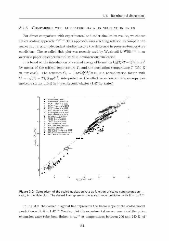
3.4. Results and discussion
3.4.6 Comparison with literature data on nucleation rates
For direct comparison with experimental and other simulation results, we choose
Hale’s scaling approach.45,47,48 This approach uses a scaling relation to compare the
nucleation rates of independent studies despite the difference in pressure-temperature
conditions. The so-called Hale plot was recently used by Wyslouzil & Wolk 154 in an
overview paper on experimental work in homogeneous nucleation.
It is based on the introduction of a scaled energy of formation C0(Tc/T −1)3/(lnS)2
by means of the critical temperature Tc and the nucleation temperature T (350 K
in our case). The constant C0 = [16π/3]Ω3/ ln 10 is a normalization factor with
Ω = γ/(Tc − T )/(kBρ2/3l ) interpreted as the effective excess surface entropy per
molecule (in kB units) in the embryonic cluster (1.47 for water).
0 5 10 15 20 25 30
0
5
10
15
20
25
30
C0 (T
c/T−1)
3 / (lnS)
2
− lo
g (
J /
10
26 c
m−
3s
−1 )
current work TIP4P
current work TIP4P/2005
PEWT Holten et al. 2005
PEWT Fransen et al. 2015
PEWT Luijten et al. 1997
NPC Viisanen et al. 1993
SSN Wyslouzil et al. 2007
LFDC Manka et al. 2010
FEC Manka et al. 2007
TDCC Brus et al. 2009
TDCC Brus et al. 2008
ECC Miller et al. 1983
NPC Wolk and Strey 2001
SSN Kim et al. 2004
MD SPC/E Tanaka et al. 2014
MD SPC/E Angelil et al. 2015
MD TIP4P/2005 Perez 2011
Figure 3.9: Comparison of the scaled nucleation rate as function of scaled supersaturationratio, in the Hale plot. The dashed line represents the scaled model prediction with Ω = 1.47. 46
In Fig. 3.9, the dashed diagonal line represents the linear slope of the scaled model
prediction with Ω = 1.47.46 We also plot the experimental measurements of the pulse
expansion wave tube from Holten et al.58 at temperatures between 200 and 240 K, of
54

Chapter 3. Nucleation of TIP4P and TIP4P/2005 water model
Fransen et al. 36 at 240 K, of Luijten et al.86 at 230 and 250 K, the nucleation pulse
chamber data of Viisanen et al.138 at 260 K, the supersonic nozzle data of Wyslouzil
et al. 153 at 200-230 K, the laminar flow diffusion chamber data of Manka et al. 89
at 240-270 K, the free expansion chamber data of Manka et al. 88 at 200-250 K, the
thermal diffusion cloud chamber data of Brus et al.16,18,19 from 290 to 320 K, Miller
et al. 97 from 230 to 290 K, the expansion chamber data of Wolk & Strey 152 at 220-260
K, the supersonic nozzle data of Kim et al. 75 at 210-230 K, the MD SPC/E results of
Tanaka et al.130 and Angelil et al.5 at 300-390 K and the MD TIP4P/2005 results of
Perez et al.116 at 330 K. All the measurement data use the experimentally determined
value Tc = 647.1 K, whereas the models TIP4P and TIP4P/2005 predict 588 K and
640 K,135 respectively. Thus, for the simulation data we adopt the value corresponding
to the potential model.
All experimental and numerical data tend to collapse onto or approach the prediction
line. Our data are at relatively high nucleation rates and are consistent with the data
of Tanaka, Angelil and Perez.
3.5 Conclusions
The nucleation behavior of water in Argon was investigated through MD simulations
typically covering 1250 ps and beyond. Rapid cool down from 1000 K to 350 K was
performed. Two water models, TIP4P and TIP4P/2005 were used.
We found that the stability of any cluster, even if large, strongly depends on the
energetic interactions with its surrounding molecules. By carefully tracing the structure
of the largest surviving cluster over time, we have seen that almost all its initial
molecules evaporated. The molecular composition of a large stable cluster changes
considerably throughout nucleation phase.
Following the threshold method of Yasuoka & Matsumoto 156 the MD nucleation
rates were derived. We found the nucleation rate to be 1.08 × 1027 cm−3s−1 for
TIP4P. Remarkably, the number is very close to that of Yasuoka & Matsumoto 156 ,
in spite of the fact that they used a different value for the cutoff radius, a different
cluster definition, combination rules and MD software. We found that the TIP4P/2005
prescribes a faster dynamics, with a nucleation rate of J = 2.30× 1027 cm−3s−1, which
is two times larger than TIP4P and has larger number of clusters formed.
To compare the results of the threshold method with CNT, the supersaturation
and thus the non-equilibrium value for the water density is needed. This value was
derived from MD water monomer density. We obtained relatively high supersaturations
55

3.6. Appendix
of 7.70 and 48.77 for TIP4P and TIP4P/2005, respectively. Substitution of these
values into CNT together with TIP4P and TIP4P/2005 equilibrium parameters from
literature shows that CNT overestimates the TIP4P nucleation rates by half an order
of magnitude with respect to the threshold method. The discrepancy is largest for
TIP4P/2005, which can be attributed to the poor vapor description of the water model.
The computation of nucleation rates and supersaturations allowed to compare our
data with literature data in a so-called Hale plot. We found that our results complement
existing data towards high supersaturations and nucleation rates. In the same time,
our results are consistent with those by Tanaka, Angelil and Perez.
3.6 Appendix
To prove that our nucleation simulations are not situated in the spinodal regime of
water, we make use of the IAPWS-95 formulation.143 In Fig. 3.10, we plot the spinodal
and the binodal line in the P-d diagram of the experimental water represented by
IAPWS-95. The saturation points from Vega & de Miguel 136 of TIP4P and TIP4P/2005
model are also plotted here. It is easily noticeable that both water potentials provide a
fairly good description of the vapor-liquid equilibria at these conditions.
0 0.005 0.01 0.015 0.02 0.025 0.030
5
10
15
20
25
density [g/cm3]
pre
ssu
re [
ba
r]
spinodal line
binodal line
t=0 ps
t=1250 ps TIP4P
t=1250 ps TIP4P/2005
sat. points TIP4P
sat. points TIP4P/2005
Figure 3.10: Pressure-density diagram of water from IAPWS-95 equation of state: binodalcurve (solid line) and spinodal curve (dashed line). The saturation points of TIP4P (dots) andTIP4P/2005 (crosses) from Vega & de Miguel 136 . The starting pressure in the MD simulations(circle), end pressure of TIP4P (plus sign) and of TIP4P/2005 (triangle).
Knowing the water density in our simulations (ρW = 0.006806 g/cm3) and the
56
Chapter 3. Nucleation of TIP4P and TIP4P/2005 water model
pressure, we pin-point the start (t = 0 ps) and end point (t = 1250 ps) of the nucleation
simulations. All values are away from the spinodal line, confirming that the initial
and final state of the nucleation simulations are in the water metastable regime. Note
that the starting pressure is the same in both water model systems. The pressure at
the end of the TIP4P simulations is higher than of the TIP4P/2005 due to the lower
number of clusters formed during the simulation time.
57

3.6. Appendix
58

4Water nucleation in helium, methane, argon,
and carbon dioxide∗
4.1 Introduction
Understanding and modeling condensation phenomena plays a crucial role in the field
of earth sciences,120,13 biomedical research,8,106 and industrial processes such as the
production of liquefied natural gas (LNG). Prior to liquefaction, impurities like water
vapor, carbon dioxide, and hydrogen sulfide need to be removed to avoid blockages in
the pipelines and heat exchangers, and to prevent damage to the liquefaction equipment.
Several removal procedures are available,76 but none of them effectively covers all types
and concentrations of contaminants. Here, we investigate the condensation of water as
a first step in a gas treatment process.
Nucleation is the first stage in the condensation process and is subsequently followed
by droplet growth. The nucleation process is called homogeneous when the presence of
dust particles and foreign bodies can be excluded and small nuclei of the new phase
are formed solely due to statistical thermal fluctuations within the metastable phase.
∗The content of this chapter is based on the following publication: Dumitrescu, L.R.,Huinink, H., Smeulders, D.M.J., Dam, J.A.M, and Gaastra-Nedea, S.V., Water nucleation inhelium, methane, and argon: a molecular dynamics study, The Journal of Chemical Physics,148, 194502 (2018), with an additional section on preliminary results of water nucleation incarbon dioxide and methane.
59

4.1. Introduction
These fluctuations need to overcome an energy barrier in order to form an interface
between the gas phase and the new stable nucleus. The height of the nucleation barrier
decreases as the degree of supersaturation increases. The supersaturation is defined
as S = ρn/ρnsat, where ρn and ρnsat are the number densities of the supersaturated
vapor and saturated vapor at identical conditions, respectively. The nucleation rate
(J) is defined as the amount of stable (critical) clusters formed per unit time, per unit
volume.
When a cluster catches a new water molecule, it absorbs the latent heat, which
subsequently raises the temperature of the cluster. This leads to non-isothermal
conditions in the system and highly affects the nucleation rate of the process (as
nucleation is very sensitive to temperature changes). In experimental or real-life plants,
a carrier gas typically removes the heat through high-frequency molecular collisions. It
seems obvious that the more efficiently the latent heat is removed from the cluster,
the more the nucleation rate will approach the isothermal nucleation rate, at which
point no latent heat is generated at all. Gas pressure also influences nucleation. An
early study reported a pressure effect of the carrier gas on nucleation in a thermal
diffusion cloud chamber setup.35 The pressure effect has been intensively studied both
theoretically and experimentally; a detailed review is given by Brus et al. 17 Still, both
theoretical model predictions and experimental results are very much controversial.
Improved formulations of the classical nucleation theory (CNT11,139,31,38,158) agree on
nucleation rates decreasing with increasing pressure of the carrier gas,34,80,69 but Feder
et al. 32 report the opposite effect. Experimental data show nucleation rates either
increase, decrease, or do not vary at all when the carrier gas pressure increases.148
The influence of the carrier gas density was previously investigated in molecular
dynamics (MD) simulations of argon nucleation by Wedekind et al. 150 The authors
report an overall increase in nucleation rates with an increasing amount of helium.
Their result is consistent with the studies on water nucleation by Zipoli et al. 161 at
350 K using the coarse grain TIP4P model in argon and of Tanaka et al. 130 using
the SPC/E water model in argon and temperatures of 275 to 350 K. Monte Carlo
simulations were performed to compute the nucleation barrier of water cluster formation
in nitrogen,109 where it was found that the nucleation barrier at 240 K increased in
relation to increases in carrier gas density, while at 298.15 K no effect was found.
The role of the carrier gas type was investigated experimentally in a laminar flow
diffusion chamber for n-hexanol nucleation.85 The nucleation rates were found to be
larger for argon than for helium, with reduced differences at elevated temperatures.
However, the nucleation pulse chamber experiments on water nucleation by Viisanen
60
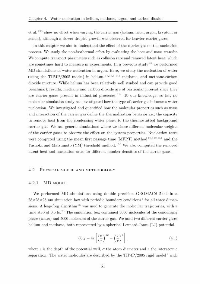
Chapter 4. Water nucleation in helium, methane, argon, and carbon dioxide
et al. 138 show no effect when varying the carrier gas (helium, neon, argon, krypton, or
xenon), although a slower droplet growth was observed for heavier carrier gases.
In this chapter we aim to understand the effect of the carrier gas on the nucleation
process. We study the non-isothermal effect by evaluating the heat and mass transfer.
We compute transport parameters such as collision rate and removed latent heat, which
are sometimes hard to measure in experiments. In a previous study28 we performed
MD simulations of water nucleation in argon. Here, we study the nucleation of water
(using the TIP4P/2005 model) in helium,17,36,6,141 methane, and methane-carbon
dioxide mixture. While helium has been relatively well studied and can provide good
benchmark results, methane and carbon dioxide are of particular interest since they
are carrier gases present in industrial processes.114 To our knowledge, so far, no
molecular simulation study has investigated how the type of carrier gas influences water
nucleation. We investigated and quantified how the molecular properties such as mass
and interaction of the carrier gas define the thermalization behavior i.e., the capacity
to remove heat from the condensing water phase to the thermostatted background
carrier gas. We ran generic simulations where we chose different molecular weights
of the carrier gases to observe the effect on the system properties. Nucleation rates
were computed using the mean first passage time (MFPT) method10,149,151 and the
Yasuoka and Matsumoto (YM) threshold method.155 We also computed the removed
latent heat and nucleation rates for different number densities of the carrier gases.
4.2 Physical model and methodology
4.2.1 MD model
We performed MD simulations using double precision GROMACS 5.0.4 in a
28×28×28 nm simulation box with periodic boundary conditions4 for all three dimen-
sions. A leap-frog algorithm56 was used to generate the molecular trajectories, with a
time step of 0.5 fs.28 The simulation box contained 5000 molecules of the condensing
phase (water) and 5000 molecules of the carrier gas. We used two different carrier gases
helium and methane, both represented by a spherical Lennard-Jones (LJ) potential,
ULJ = 4ε
[(σr
)12
−(σr
)6], (4.1)
where ε is the depth of the potential well, σ the atom diameter and r the interatomic
separation. The water molecules are described by the TIP4P/2005 rigid model1 with
61

4.2. Physical model and methodology
Table 4.1: Potential parameters and densities of carrier gases and water. The parameters formethane from Ref. CH4FF, for helium are from Ref. Bird, and for the TIP4P/2005 water modelfrom Ref. tip4p2005.
Atom/Molecule ε/k (K) σ (A) qH (e) ρ (mg cm−3)
CH4 148.55 3.7281 - 6.060Ar 119.8 3.405 - 15.093He 10.22 2.576 - 1.512TIP4P/2005 93.2 3.1589 +0.5564 6.806
an intermolecular potential having the following expression:
Uinter =∑a,b<a
4εOO
[(σOOrab
)12
−(σOOrab
)6]
+1
4πε0
∑i,j<i
qiqjrij
. (4.2)
The first summation represents the LJ interaction between the oxygen atoms of the
water molecule, where εOO, σOO, and rab are the interaction strength, the length scale,
and the distance between the oxygen atoms, respectively. The second summation
represents the electrostatic potential, where ε0 is the electric constant, qi and qj are the
partial charges, and rij the distances between the pairs of charged sites in the water
molecule.
The LJ and the short-range Coulombic interactions were both truncated at a cut-off
distance, rcut, of 99 A. The Particle-Mesh Ewald (PME)27 technique was used for the
long-range Coulombic interactions. Lorentz-Berthelot combining rules were assumed
between unlike atoms i and j, with σij = (σii + σjj)/2 and εij =√εiiεjj . A water
molecule was assumed to interact with the carrier gas only through its oxygen site.
In Table 4.1 the values of the potential parameters and the starting densities are
given (note that densities change during nucleation). For reference, the values for
argon are also included here, as this gas was used in our previous publication.28 In the
forthcoming, the validation of the force fields (FFs) of water and carrier gases at the
nucleation temperature of 350 K is presented.
4.2.2 System and model parameters
For validation of the nucleation mechanism we examined the water density of the
TIP4P/2005 model (Table 4.1) for metastability. MD simulations were carried out
in an NVT (i.e. constant number of particles, volume, and temperature) ensemble
containing 2500 water molecules at 350 K and densities in the range of 3 to 33 mg
62
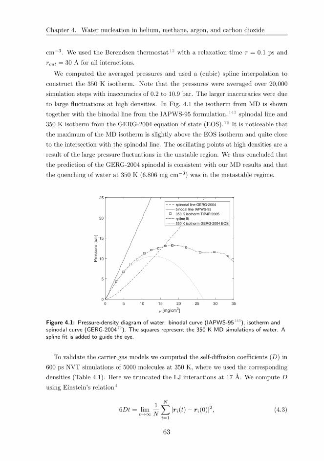
Chapter 4. Water nucleation in helium, methane, argon, and carbon dioxide
cm−3. We used the Berendsen thermostat12 with a relaxation time τ = 0.1 ps and
rcut = 30 A for all interactions.
We computed the averaged pressures and used a (cubic) spline interpolation to
construct the 350 K isotherm. Note that the pressures were averaged over 20,000
simulation steps with inaccuracies of 0.2 to 10.9 bar. The larger inaccuracies were due
to large fluctuations at high densities. In Fig. 4.1 the isotherm from MD is shown
together with the binodal line from the IAPWS-95 formulation,143 spinodal line and
350 K isotherm from the GERG-2004 equation of state (EOS).79 It is noticeable that
the maximum of the MD isotherm is slightly above the EOS isotherm and quite close
to the intersection with the spinodal line. The oscillating points at high densities are a
result of the large pressure fluctuations in the unstable region. We thus concluded that
the prediction of the GERG-2004 spinodal is consistent with our MD results and that
the quenching of water at 350 K (6.806 mg cm−3) was in the metastable regime.
0 5 10 15 20 25 30 35
ρ [mg/cm3]
0
5
10
15
20
25
Pre
ssu
re [
ba
r]
spinodal line GERG-2004
binodal line IAPWS-95
350 K isotherm TIP4P/2005
spline fit
350 K isotherm GERG-2004 EOS
Figure 4.1: Pressure-density diagram of water: binodal curve (IAPWS-95 143), isotherm andspinodal curve (GERG-2004 79). The squares represent the 350 K MD simulations of water. Aspline fit is added to guide the eye.
To validate the carrier gas models we computed the self-diffusion coefficients (D) in
600 ps NVT simulations of 5000 molecules at 350 K, where we used the corresponding
densities (Table 4.1). Here we truncated the LJ interactions at 17 A. We compute D
using Einstein’s relation4
6Dt = limt→∞
1
N
N∑i=1
|ri(t)− ri(0)|2, (4.3)
63

4.2. Physical model and methodology
where the right-hand side represents the mean squared displacement (MSD) over
all atoms, with N being the number of atoms and ri the position of the atom i
at time t. The diffusion coefficient is obtained from the least squares regression of
the MSD. The coefficients were averaged over five independent runs, and the results
were DHe = (19.7 ± 0.4) × 10−8 cm2 s−1, DCH4= (2.78 ± 0.04) × 10−8 cm2 s−1
and DAr = (2.23 ± 0.03) × 10−8 cm2 s−1. The corresponding REFPROP84 data
are DHe = (22.2± 1.6)× 10−8 cm2 s−1, DCH4= (2.89± 0.09)× 10−8 cm2 s−1, and
DAr = (2.57 ± 0.06) × 10−8 cm2 s−1. The REFPROP values were within the error
bars of the MD data for CH4 and slightly outside for He and Ar. Such discrepancies
were reported before for Ar.73
To define condensation, water clusters consisting of two or more water molecules
need to be identified. For this we used Stillinger’s definition,128 who argued that two
atoms belong to a cluster if their centers of mass are within a fixed distance rS . We
assumed that a water cluster is formed if the distance between two oxygen atoms
becomes less than 3.7 A (∼1.17σO−O).28
4.2.3 Computational approach for nucleation rates
We initially equilibrated the systems over 200 ps during which the gas mixture
reached a stable set temperature of 1000 K and pressure of 63 bar. We first used
a Berendsen thermostat12 for this temperature (between 0 - 100 ps) and next used
a Berendsen barostat for this pressure (between 100 - 200 ps), both with relaxation
time of τ = 0.1 ps. After applying the barostat the volume of (28 nm)3 changed by a
maximum of 0.25 %, which was considered negligible. Next, a 200 ps microcanonical
ensemble was used to verify the energy drift of the unperturbed system (between 200 -
400 ps). Then the condensation was triggered by an instantaneous temperature drop
(quenching) to 350 K by simple velocity rescaling. During the subsequent condensation
period, the carrier gas was kept at 350 K by means of a velocity rescaling thermostat
(with τ = 0.025 ps) and water was not coupled to any thermostat. Condensation was
simulated for a period of 1250 ps.155
In Fig. 4.2a we show a characteristic number density distribution at the end of
the simulation run. In Fig. 4.2b the density distribution in half plane cross sections
is shown. We notice in Fig. 4.2a that clusters are formed and in Fig. 4.2b that the
maximum number density inside a cluster reached approximately 3×10⁻⁴ nm−3, which
is in good agreement with the bulk liquid number density of water143 (2.9 × 10⁻⁴
nm−3).
We computed the nucleation rates by employing two different methods: the threshold
64

Chapter 4. Water nucleation in helium, methane, argon, and carbon dioxide
ρ110-4 nm-3
1
2
3
4
5
6
(a)
ρ110-4 nm-3
0.5
1.0
1.5
2.0
2.5
3.0
(b)
Figure 4.2: Number density distribution (a) in the simulation box and (b) in half plane cross-sections of the box.
method of Yasuoka & Matsumoto 155 (YM method) and the mean first passage time
(MFPT) method introduced by Wedekind et al. 151
The YM method is particularly suited to compute nucleation rates in large and
highly supersaturated systems,23 where a significant number of clusters is rapidly
formed. The method is based on snapshots of cluster size distributions. From the
distributions, the number of clusters larger than a threshold value (nth) is plotted over
time, in which the threshold value should be larger than the critical size. Because we
do not have a priori information on the critical cluster size, we choose an arbitrary
range of values for nth.
In Figs. 4.3a and 4.3b we plot the averaged time evolution of the number of water
clusters in helium and methane for different nth. The averaging is over 6 independent
runs. During steady-state nucleation, the number of clusters increases linearly with
time. This linear regime is followed by a plateau and a subsequent decrease, which
suggests that nucleation stopped and droplet growth took over. Straight lines are
fitted through the data points in the nucleation regime in the same way as in our
previous publication.28 For any nth larger than the critical cluster size, we expect the
lines to run in parallel. According to the YM method,155 the nucleation rate can be
determined from the slope of the fitted lines and the simulation box volume. These
lines are not parallel for helium, nor for methane. To compute the nucleation rates
we used individual and averaged slopes. The decrease in the slopes of the lines is
attributable to the high supersaturation conditions, where a large number of small
clusters are initially formed that later coalesce and grow into larger clusters.
65

4.2. Physical model and methodology
0 200 400 600 800 1000 1200
0
5
10
15
20
25
30
35
40
Num
ber
of w
ate
r clu
ste
rs
Time [ps]
in Helium
Fit
n ≥ 20
n ≥ 30
n ≥ 40
n ≥ 50
(a)
0 200 400 600 800 1000 1200
0
5
10
15
20
25
30
35
40
Num
ber
of w
ate
r clu
ste
rs
Time [ps]
in Methane
Fit
n ≥ 20
n ≥ 30
n ≥ 40
n ≥ 50
(b)
Figure 4.3: Averaged time development of water cluster thresholds ‘n’ in (a) helium (b)methane. In both figures ‘n’: larger than 20, 30, 40, and 50 molecules. Solid lines are fittingsused to measure the nucleation rate.
In Fig. 4.4 we show the number of water monomers in methane and helium. To
compute ρn we averaged the number of monomers between 300 and 700 ps.28 Using
the TIP4P/2005 saturated density136 (ρnsat = 2× 10⁻³ nm−3) at 350 K, the systems
had supersaturations S = 51.82 in helium and S = 44.50 in methane. These supersatu-
rations are considerably higher than S = 11.96 in helium and S = 10.27 in methane
when using the literature data143 (ρnsat = 8.7× 10⁻³ nm−3), as was also observed by
Perez & Rubio 116 .
At supersaturations of 51.82 (11.96 corresponding literature data) in helium and
44.50 (10.27) in methane the CNT predictions of the nucleation barriers become 2.16
kBT (5.40) for helium and 2.33 kBT (6.13) for methane, showing that the nucleation
mechanism prevails. Moreover, the critical cluster size is 1.09 (4.35) for He and 1.22
(5.27) for CH4, with nucleation rates of 4.44 (613)×1028 cm−3 s−1 in helium and 2.74
(172)×1028 cm−3 s−1 in methane.
To analyze the evolution of the mechanism in our simulations we included typical
cluster distributions at three moments. In Fig. 4.5 at 20 ps (top figure) we notice very
small clusters were formed, while later at 300 ps and 700 ps they grew and coalesced
into larger clusters.
Another way to compute the nucleation rate is the so-called MFPT method.49 In
this approach, the time until the largest cluster in the system reaches a given cluster
size n is recorded. Next, from the averaged time over replicated simulations the mean
first passage time, τ(n), is obtained. The approach is particularly suited for the study
of nucleation in relatively small system sizes and high free-energy barriers. Under these
66
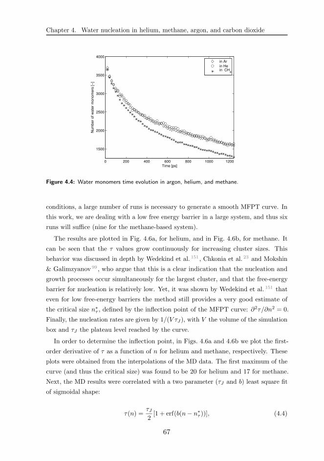
Chapter 4. Water nucleation in helium, methane, argon, and carbon dioxide
0 200 400 600 800 1000 1200
1500
2000
2500
3000
3500
4000
Nu
mb
er
of
wa
ter
mo
no
me
rs [
−]
Time [ps]
in Ar
in Hein CH
4
Figure 4.4: Water monomers time evolution in argon, helium, and methane.
conditions, a large number of runs is necessary to generate a smooth MFPT curve. In
this work, we are dealing with a low free energy barrier in a large system, and thus six
runs will suffice (nine for the methane-based system).
The results are plotted in Fig. 4.6a, for helium, and in Fig. 4.6b, for methane. It
can be seen that the τ values grow continuously for increasing cluster sizes. This
behavior was discussed in depth by Wedekind et al. 151 , Chkonia et al. 23 and Mokshin
& Galimzyanov 99 , who argue that this is a clear indication that the nucleation and
growth processes occur simultaneously for the largest cluster, and that the free-energy
barrier for nucleation is relatively low. Yet, it was shown by Wedekind et al. 151 that
even for low free-energy barriers the method still provides a very good estimate of
the critical size n∗τ , defined by the inflection point of the MFPT curve: ∂2τ/∂n2 = 0.
Finally, the nucleation rates are given by 1/(V τJ ), with V the volume of the simulation
box and τJ the plateau level reached by the curve.
In order to determine the inflection point, in Figs. 4.6a and 4.6b we plot the first-
order derivative of τ as a function of n for helium and methane, respectively. These
plots were obtained from the interpolations of the MD data. The first maximum of the
curve (and thus the critical size) was found to be 20 for helium and 17 for methane.
Next, the MD results were correlated with a two parameter (τJ and b) least square fit
of sigmoidal shape:
τ(n) =τJ2
[1 + erf(b(n− n∗τ ))], (4.4)
67

4.3. Results and discussions
3 10 20 30 60 1000
20
40
60
80
At 20 ps
Num
ber
of clu
ste
rs [−
]
Cluster size [−]
10 20 30 60 100 120
0
1
2
3
At 300 ps
Num
ber
of clu
ste
rs [−
]
Cluster size [−]
10 20 30 60 100 120
0
1
2
3
At 700 ps
Num
ber
of clu
ste
rs [−
]
Cluster size [−]
Figure 4.5: Cluster size distribution at 20 ps, at 300 ps and 700 ps.
where erf() is the error function and b is defined by the Zeldovich factor158 Z = b/√π.
The fitting domain is between n = 0 and nmax = 2× n∗, which corresponds to τ = 329
ps for helium and τ = 243 ps for methane. As starting points for τJ we used the
aforementioned τ values and for b we use zero. In Figs. 4.6a and 4.6b, the resulting
curves are plotted (solid lines). Convergence was reached in 6-7 iterations, with values
of τJ = 330 ps and b = 0.079 for helium and τJ = 215 ps and b = 0.096 for methane.
We used these values to compute the nucleation rates, which are discussed in the
following section.
4.3 Results and discussions
4.3.1 Nucleation rates
In Table 4.2 we define the notations and the starting density values of the systems.
Here, we also added simulations at a slightly lower water density (4.903 mg cm−3) and
68

Chapter 4. Water nucleation in helium, methane, argon, and carbon dioxide
0 10 20 30 40 50 60 70 80 900
100
200
300
400
500
600
Cluster size (n)
τ(n
) [ps]
τJ
0 10 20 30 40 50 60 70 80 900
2
4
6
8
10
12
∂ τ
(n)/
∂ n
n*
τ
τ(n) MD data
τ(n) fit
∂ τ (n)/ ∂ n
(a)
0 10 20 30 40 50 60 70 80 900
100
200
300
400
500
600
Cluster size (n)
τ(n
) [ps]
τJ
0 10 20 30 40 50 60 70 80 900
2
4
6
8
10
12
∂ τ
(n)/
∂ n
n*
τ
τ(n) MD data
τ(n) fit
∂ τ (n)/ ∂ n
(b)
Figure 4.6: (a) MFPT (τ) and first derivative ∂τ(n)/∂n as function of the cluster size inhelium, (b) in methane.
Table 4.2: MD systems and densities (ρ) in mg cm−3 from the type and number of moleculesof the carrier gas.
Carrier gas \ molec 5000∗ 5000† 10000† 15000†
HeliumS0,He S1,He S2,He S3,He
5.99 8.32 9.83 11.34
MethaneS0,CH4 S1,CH4 S2,CH4 S3,CH4
9.27 12.87 18.93 24.99
Argon- S1,Ar - -- 21.90 - -
Note: All systems contain 5000 water molecules.∗ρH2O = 4.903 mg cm−3
†ρH2O = 6.806 mg cm−3
higher carrier gas concentrations.
In Table 4.3 the nucleation rates are given. We obtained J = 20.4 ± 1.1 × 1026
cm−3s−1 for helium and 28.2±0.9×1026 cm−3s−1 for methane, where we averaged over
three different slopes nth = 30, 40, and 50 (see Fig. 4.3). The values from the individual
threshold lines are also given in Table 4.3. The uncertainties of the MFPT rates were
obtained from the standard deviation of τ(n) and those of the YM method from the
variation of the slopes. Notice that the nucleation rates decreased with increasing nth.
The nucleation rates obtained from MFPT were typically one order of magnitude lower
than those obtained from the YM method, as was also found in the study by Romer
& Kraska 122 for zinc nucleation in argon. The authors attributed this discrepancy to
69

4.3. Results and discussions
Table 4.3: MD Nucleation rate (J) values in 1026 cm−3s−1 of water in helium, methane, andargon at 350 K.
Method S0,He S1,He S2,He S3,He S1,Ar S0,CH4 S1,CH4 S2,CH4 S3,CH4
YM30,40,50 20.4± 1.1 28.5 42.6 23.0± 1.0 28 28.2± 0.9 36.9 49.5YM20 29.1± 1.1 - 42.8± 0.9YM30 22.6± 1.3 25.7± 0.9 35.5± 1.0YM40 19.3± 1.2 22.9± 1.0 25.9± 0.8YM20,30,40 10.4 14.1MFPT 0.76 1.37± 0.16 1.71± 0.50 1.02 2.08± 0.27
the coupling of the nucleation and growth processes. The MFPT method considers
only the largest cluster. Thus, if this cluster is already in growth stage, the method
will overestimate the size of the critical cluster and underestimate the nucleation rate.
Yet, the MFPT method predicted a critical cluster size of 20 for helium and of 17 for
methane. From this we can confirm that the choice of the threshold values nth in the
YM method was indeed correct, as these threshold values should be larger than the
critical cluster size.
Remarkably, the three carrier gases (helium, argon, and methane) had similar
nucleation rates in spite of the differences in molecular weight and interaction model
parameters (see Table 4.1). The reason for this similarity is discussed in the next
subsection.
4.3.2 Thermalization by the carrier gas
The removal of latent heat (thermalization) from the clusters is highly dependent
on the collision rate of the clusters with the surrounding carrier molecules. In the
study by Wedekind et al. 150 on the influence of the carrier gas on argon nucleation,
the authors argue that a lighter carrier gas is expected to show better thermalization
characteristics than heavier gas, due to higher collision frequency with clusters. The
statement is based on the theoretical prediction of Feder et al. 32 for monoatomic
vapors and gases. We address this statement by comparing the collision rates, removed
energy, and nucleation rates for our three different carrier gases in the S1 systems.
We computed binary water-carrier gas collision rates (vcw) averaged over the first
600 ps after the quenching with 1 ps time step and we defined a collision by an
intermolecular distance smaller than 1.12σ. The removed energy (Q) was computed
by subtracting the final total energy (at 1.25 ns) from the initial total energy. As the
energy in the system is transferred not only through collisions between carrier gas and
water molecules but also between the carrier gas molecules among themselves, we also
considered the carrier-carrier gas collision rates (vcc), which were also averaged over the
70

Chapter 4. Water nucleation in helium, methane, argon, and carbon dioxide
first 600 ps. The results are given in Table 4.4. We note that the slight discrepancies
between nucleation rates are correlated with the amount of removed energy and with
the water-carrier gas and carrier-carrier gas collision rates. It seems, then, that the
removal of energy is not governed by the molecular mass of the carrier gas (mc), as
the largest energy removal was found for CH4 with a mass ratio between Ar and He.
Obviously, these carrier gases differ in other properties as well (see Table 4.1), which
could also have an effect on the removal of energy.
Table 4.4: Computational results and reduced mass of the carrier gases, with JYM being thenucleation rate from the YM method.
Carrier gas CH4 Ar He
JYM(30,40,50) (1026 cm−3s−1) 28.2 23.0 20.4
Q (104 RT) 3.54 2.96 2.79vcc (ps−1) 79 60 32vwc (ps−1) 56 53.5 44mc/mH2O 0.89 2.22 0.22
We further investigated the mass dependency of water-carrier collision rates and
removed energy by varying mc whilst keeping the other properties of the carrier gases
the same. The results are given in Fig. 4.7. We notice that for variations of mc,
the trends of binary collision rates and energy removal contrast; a larger molecular
mass led to higher collisions but lower heat transfer. The lower heat transfer of the
heavier carrier gas can be explained through an analytical derivation of the center of
mass translational post-collision velocities of water molecules; this was also reported
in Nedea et al. 104 The water-carrier collisions consist of interactions of carrier gas
molecules not solely with water nuclei but also with water monomers. Due to the low
energy transfer, a heavier carrier gas encounters more water monomers and smaller
water clusters to collide with compared to a lighter carrier gas. Thus, the different
cluster and monomer distribution evolution in our systems led to differences in the
collision rates. Hence, from our simulations the thermalization dependency on mc is in
agreement with Wedekind’s statement, as long as the interaction parameters are kept
constant.
Figure 4.7 also shows that QCH4 > QAr > QHe and that vCH4wc > vArwc > v He
wc for
corresponding molecular masses. In Table 4.5 the nucleation rates for all these masses
are shown. From this table we notice that JCH4> JAr > JHe, except for the highest
mass ratio 22.22, where the computation of J becomes ambiguous. At this point we
can argue that the mass of the carrier gas is not the only factor in thermalization, but
71

4.3. Results and discussions
10−1
100
101
102
0.6
1.1
1.6
2.1
2.6
3.1
3.6
4.1x 10
4
En
erg
y r
em
ove
d b
y c
arr
ier
ga
s [
RT
]
mc/m
H2O
[−]
10−1
100
101
10240
45
50
55
60
65
70
75
Wa
ter−
ca
rrie
r co
llisio
n r
ate
s [
ps−
1]
CH4
Ar
He
Figure 4.7: Removed energy and collision rates as function of the reduced mc. Open circlesrepresent true values.
the interaction parameters σ and ε also play a certain role. Additional simulations were
performed where we changed the interaction strength (ε) and kept the other properties
unchanged. In Fig. 4.8 we can observe that the increasing strength of the interactions
led to higher energy removal in all carrier gases.
Table 4.5: Comparison of water nucleation rates for different molecular mass of argon, helium,and methane. Note that the JYM in helium at largest mass could not be computed due tosparse data points.
JYM(30,40,50) (1026 cm−3s−1)mc/mH2O
0.22 0.89 2.22 22.22
CH4 30.2 28.2 24.4 3.21Ar 27.9 26.7 23.0 10.8He 20.4 14.9 11.0 -
Finally, the interplay between mass and interaction parameters of the carrier gases
support the small discrepancies in the nucleation rates. This explains why the optimal
parameter values of CH4 lead to the largest nucleation rate.
4.3.3 Effect of the carrier gas concentration
The effect of the carrier gas concentrations on the latent heat removal for different
carrier gases was investigated. The number of water molecules in the computational
72
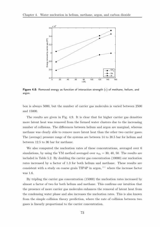
Chapter 4. Water nucleation in helium, methane, argon, and carbon dioxide
0 20 40 60 80 100 120 140 1602.4
2.6
2.8
3
3.2
3.4
3.6x 10
4
ε [K]
En
erg
y r
em
ove
d b
y c
arr
ier
ga
s [
RT
]
CH4
He
Ar
Figure 4.8: Removed energy as function of interaction strength (ε) of methane, helium, andargon.
box is always 5000, but the number of carrier gas molecules is varied between 2500
and 15000.
The results are given in Fig. 4.9. It is clear that for higher carrier gas densities
more latent heat was removed from the formed water clusters due to the increasing
number of collisions. The differences between helium and argon are marginal, whereas
methane was clearly able to remove more latent heat than the other two carrier gases.
The (average) pressure range of the systems are between 14 to 38.5 bar for helium and
between 12.5 to 36 bar for methane.
We also computed the nucleation rates of these concentrations, averaged over 6
simulations, by using the YM method averaged over nth = 30, 40, 50. The results are
included in Table 5.2. By doubling the carrier gas concentration (10000) our nucleation
rates increased by a factor of 1.3 for both helium and methane. These results are
consistent with a study on coarse grain TIP4P in argon,161 where the increase factor
was 1.6.
By tripling the carrier gas concentration (15000) the nucleation rates increased by
almost a factor of two for both helium and methane. This confirms our intuition that
the presence of more carrier gas molecules enhances the removal of latent heat from
the condensing water phase and also increases the nucleation rates. This is also known
from the simple collision theory prediction, where the rate of collision between two
gases is linearly proportional to the carrier concentration.
73
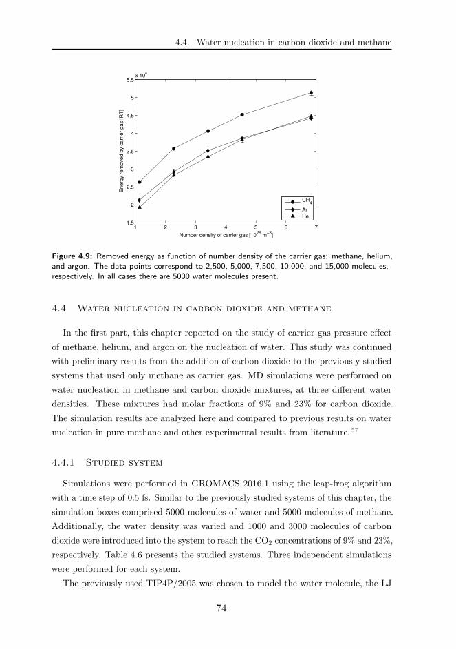
4.4. Water nucleation in carbon dioxide and methane
1 2 3 4 5 6 71.5
2
2.5
3
3.5
4
4.5
5
5.5x 10
4
Number density of carrier gas [1026
m−3
]
En
erg
y r
em
ove
d b
y c
arr
ier
ga
s [
RT
]
CH4
Ar
He
Figure 4.9: Removed energy as function of number density of the carrier gas: methane, helium,and argon. The data points correspond to 2,500, 5,000, 7,500, 10,000, and 15,000 molecules,respectively. In all cases there are 5000 water molecules present.
4.4 Water nucleation in carbon dioxide and methane
In the first part, this chapter reported on the study of carrier gas pressure effect
of methane, helium, and argon on the nucleation of water. This study was continued
with preliminary results from the addition of carbon dioxide to the previously studied
systems that used only methane as carrier gas. MD simulations were performed on
water nucleation in methane and carbon dioxide mixtures, at three different water
densities. These mixtures had molar fractions of 9% and 23% for carbon dioxide.
The simulation results are analyzed here and compared to previous results on water
nucleation in pure methane and other experimental results from literature.57
4.4.1 Studied system
Simulations were performed in GROMACS 2016.1 using the leap-frog algorithm
with a time step of 0.5 fs. Similar to the previously studied systems of this chapter, the
simulation boxes comprised 5000 molecules of water and 5000 molecules of methane.
Additionally, the water density was varied and 1000 and 3000 molecules of carbon
dioxide were introduced into the system to reach the CO2 concentrations of 9% and 23%,
respectively. Table 4.6 presents the studied systems. Three independent simulations
were performed for each system.
The previously used TIP4P/2005 was chosen to model the water molecule, the LJ
74
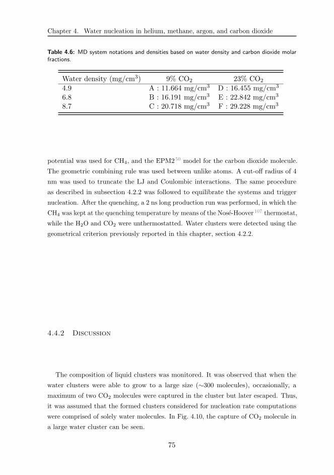
Chapter 4. Water nucleation in helium, methane, argon, and carbon dioxide
Table 4.6: MD system notations and densities based on water density and carbon dioxide molarfractions.
Water density (mg/cm3) 9% CO2 23% CO2
4.9 A : 11.664 mg/cm3 D : 16.455 mg/cm3
6.8 B : 16.191 mg/cm3 E : 22.842 mg/cm3
8.7 C : 20.718 mg/cm3 F : 29.228 mg/cm3
potential was used for CH4, and the EPM250 model for the carbon dioxide molecule.
The geometric combining rule was used between unlike atoms. A cut-off radius of 4
nm was used to truncate the LJ and Coulombic interactions. The same procedure
as described in subsection 4.2.2 was followed to equilibrate the systems and trigger
nucleation. After the quenching, a 2 ns long production run was performed, in which the
CH4 was kept at the quenching temperature by means of the Nose-Hoover107 thermostat,
while the H2O and CO2 were unthermostatted. Water clusters were detected using the
geometrical criterion previously reported in this chapter, section 4.2.2.
4.4.2 Discussion
The composition of liquid clusters was monitored. It was observed that when the
water clusters were able to grow to a large size (∼300 molecules), occasionally, a
maximum of two CO2 molecules were captured in the cluster but later escaped. Thus,
it was assumed that the formed clusters considered for nucleation rate computations
were comprised of solely water molecules. In Fig. 4.10, the capture of CO2 molecule in
a large water cluster can be seen.
75

4.4. Water nucleation in carbon dioxide and methane
Figure 4.10: Snapshot of a CO2 molecule captured in the formed water cluster.
Nucleation rates were derived by applying the YM method,155 averaged over the
three independent simulations. The time evolution of the number of clusters larger
than 20, 30, 40, and 50 is shown in Fig. 4.11 for system A and D, in Fig. 4.12 for
system B and E, and in Fig. 4.13 for system C and F. As the evolution of the number
of clusters for larger thresholds (n > 40) was inconclusive, only clusters larger than
30 and 40 molecules were used for the computation of the nucleation rates. For the
computation of the supersaturation, the vapor density (ρn) values were derived from
the monomer values averaged over the linear fitting domain, marked by the solid lines
in these figures.
0 200 400 600 800 1000 12000
5
10
15
20
25
30
Num
ber
of H
2O c
lust
ers
Time [ps]
n ≥ 20n ≥ 30n ≥ 40n ≥ 50
(a)
0 200 400 600 800 1000 12000
5
10
15
20
25
30
35
40
Num
ber
of H
2O c
lust
ers
Time [ps]
n ≥ 20n ≥ 30n ≥ 40n ≥ 50
(b)
Figure 4.11: Number of water clusters as a function of time in (a) system A and (b) in systemD.
76
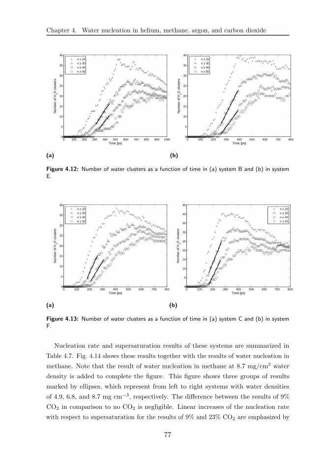
Chapter 4. Water nucleation in helium, methane, argon, and carbon dioxide
0 100 200 300 400 500 600 700 800 900 10000
5
10
15
20
25
30
35
40N
umbe
r of
H2O
clu
ster
s
Time [ps]
n ≥ 20n ≥ 30n ≥ 40n ≥ 50
(a)
0 100 200 300 400 500 600 700 8000
5
10
15
20
25
30
35
40
Num
ber
of H
2O c
lust
ers
Time [ps]
n ≥ 20n ≥ 30n ≥ 40n ≥ 50
(b)
Figure 4.12: Number of water clusters as a function of time in (a) system B and (b) in systemE.
0 100 200 300 400 500 600 700 8000
5
10
15
20
25
30
35
40
Num
ber
of H
2O c
lust
ers
Time [ps]
n ≥ 20n ≥ 30n ≥ 40n ≥ 50
(a)
0 100 200 300 400 500 600 700 8000
5
10
15
20
25
30
35
40
45
Num
ber
of H
2O c
lust
ers
Time [ps]
n ≥ 20n ≥ 30n ≥ 40n ≥ 50
(b)
Figure 4.13: Number of water clusters as a function of time in (a) system C and (b) in systemF.
Nucleation rate and supersaturation results of these systems are summarized in
Table 4.7. Fig. 4.14 shows these results together with the results of water nucleation in
methane. Note that the result of water nucleation in methane at 8.7 mg/cm3 water
density is added to complete the figure. This figure shows three groups of results
marked by ellipses, which represent from left to right systems with water densities
of 4.9, 6.8, and 8.7 mg cm−3, respectively. The difference between the results of 9%
CO2 in comparison to no CO2 is negligible. Linear increases of the nucleation rate
with respect to supersaturation for the results of 9% and 23% CO2 are emphasized by
77

4.4. Water nucleation in carbon dioxide and methane
Table 4.7: Supersaturation and nucleation rate results of water in carbon dioxide and methanesystems.
System A B C D E F
S 36.8 45.52 58.56 35.37 43.03 55.08
J (1026 cm−3s−1) 18.85 32.42 71.78 17.3 48.2 94.4
35 40 45 50 55 60
1
2
3
4
5
6
7
8
9
10
11x 10
27
Supersaturation [−]
Nuc
leat
ion
rate
[cm
−3 s−
1 ]
0% CO29% CO223% CO2
Figure 4.14: Effect of 9% and 23% carbon dioxide concentration on water nucleation rate at350 K. The ellipses mark the results of simulations at three different water densities (from leftto right 4.9, 6.8, and 8.7 mg cm−3).
dashed lines. For molar concentration of 23% CO2, the effect of CO2 is clearly visible
at 6.8 and 8.7 mg cm−3. Albeit in the same order of magnitude, the nucleation rates
at 8.7 mg cm−3 water density without CO2 increased from ∼ 7 × 1027 cm−3s−1 to
9×1027 cm−3s−1 at 23% CO2. Thus, with increasing density and thus supersaturation,
the effect of CO2 increased further on water nucleation.
4.4.3 Comparison with other results
In the work of Holten 57 , water nucleation was studied in methane and carbon
dioxide in an expansion wave tube setup at 235 K and 10 bar. In the following, we
qualitatively compare our results with the experimental results of Holten.
The systems studied by Holten contained 0% and 25% carbon dioxide. Supersatura-
78

Chapter 4. Water nucleation in helium, methane, argon, and carbon dioxide
tion for this study was computed using the first approximation in eq. 2.5, in which the
enhancement factor, defined as fe = yeqp/peq, was introduced. Equation 2.5 is repeated
here for the reader's convenience: S ≈ y/yeq. The nucleation rate results were plotted
as functions of supersaturation. Large discrepancies were found at S ≈ 9, the only
comparable supersaturation value, where the nucleation rates increased from 5.1× 10⁷
cm−3 s−1 at 0% CO2 to 1.9×1011 cm−3 s−1 at 25% CO2. However, when the nucleation
rates were plotted against the reduced partial pressure (yp/peq), which is approximately
equivalent to the supersaturation definition used in our computations, the influence of
CO2 was decreased to the same order of magnitude. Thus, the experimental results
of Holten, albeit at different temperature, pressure, and supersaturation conditions,
show qualitative agreement with our results on the effect of 23% CO2 by showing an
increase in nucleation rates within the same order of magnitude. However, the results
of our study are preliminary, and thus further investigation should be performed to
achieve better accuracy at different supersaturation conditions to draw firm conclusions
regarding the effect of CO2.
4.5 Conclusions
Molecular dynamics simulations were conducted to analyze the influence of the
molecular properties and concentration of the carrier gas on water condensation at 350
K. We used the TIP4P/2005 water model and the LJ potential for helium, methane,
and argon. We applied the mean first passage time (MFPT) and Yasuoka Matsumoto
(YM) methods to compute the nucleation rates. We found that the MFPT results were
typically one order of magnitude lower than the YM method for all carrier gases. This
is in agreement with earlier results from literature.
Surprisingly, it was found that the nucleation rates of water in the three carrier gases
did not show large differences, although those for methane were found systematically
higher. We found that these slight differences were clearly correlated with the amount
of removed latent heat and with the water-carrier gas and carrier-carrier gas molecular
collisions. Despite having a mass between argon and helium, methane led to the highest
nucleation rate showing that thermalization is not governed by the molecular mass of
the carrier gas.
We varied the molecular mass of the carrier gases while keeping the rest of the
properties constant. By increasing the mass of the carrier we found that the water-
carrier gas binary collisions increased while the heat removal decreased and thus
nucleation rates decrease as well. From the cluster distribution in these simulations
79

4.5. Conclusions
more water monomers and smaller water nuclei were found in a heavier carrier gas than
in a lighter carrier gas. Moreover, for corresponding masses, the different interaction
parameters of the carrier gases also led to discrepancies in thermalization efficiency
showing that interaction parameters also play a role in thermalization. Finally it was
shown that true methane, in comparison to argon and helium, has optimal values of
mass and interaction parameters rendering higher nucleation rates.
The concentration of the carrier gas was also varied. Upon increasing the background
concentration of the carrier gases, both the thermalization efficiency and nucleation
rates increased. For a doubled carrier gas concentration the nucleation rates increased
by a factor of 1.3, slightly less than in the study of Zipoli et al. 161whereas for tripled
carrier gas concentration the nucleation rates increased by almost a factor of two.
Preliminary results on water nucleation in methane and carbon dioxide addition
were also presented. Carbon dioxide was added in concentrations of 9% and 23% to
these systems. It was observed that very few CO2 molecules were trapped within the
water cluster, but they did escape later on. Thus, they were not considered part of
a nucleating cluster. For 9% CO2 concentration the differences in nucleation rates
were negligible compared to no CO2. However, for the 23% concentration of CO2
nucleation rates derived from the threshold method increased notably at the same order
of magnitude. Moreover, the effect of CO2 was stronger at higher supersaturation. A
qualitative comparison of our results for 23% of added CO2 with experimental results
of Holten using 25% CO2, although in different conditions, showed agreement and that
nucleation rates increased within the same order of magnitude. The results of our study
are preliminary, and thus further investigation should be performed to achieve better
accuracy at different supersaturation conditions to draw firm conclusions regarding the
effect of CO2.
80

5Carbon dioxide nucleation in methane∗
5.1 Introduction
With the ever-increasing energy demand and the new EU carbon emission target of
40% reduction in greenhouse gas emissions by 2030, our society is looking for cleaner fuel
alternatives. Among the fossil fuels, natural gas emits the least carbon dioxide (CO2)
per unit of energy produced. The CO2 concentration in geological reservoirs of natural
gas varies considerably around the globe.21 To meet the quality specification for pipeline
transport, natural gas needs to be processed such that it reaches CO2 concentrations
as low as 2-3%, while for a liquefaction facility the typical CO2 concentration must be
less than 50 ppm. The LNG pre-treatment usually comprises several removal steps
which not only add complexity to the LNG facility,76 but also has a CO2 footprint of
its own. The cost of the treatment is dependent on the composition and concentration
of the gas. However, a high CO2 content in the gas mixtures increases the treatment
costs.
In the present work we assess the approach of a single impurity phase separation step
by carefully determining phase transitions. The ultimate goal is to use this detailed
understanding to a localized CO2 separation step as part of the LNG liquefaction
process.
∗The content of this chapter is based on Dumitrescu, L.R., Smeulders, D.M.J., Dam,J.A.M, and Gaastra-Nedea, S.V., Molecular study of homogeneous carbon dioxide nucleationin methane using the EPM2 model, submitted 2019.
81
5.1. Introduction
An equation of state (EOS) provides a description of state properties of a pure
component or a mixture under given conditions. To induce and analyze phase changes in
a gas mixture, out-of-equilibrium (metastable) conditions are required. More specifically,
for condensation, a state of supersaturation of the vapor is required. The first step of
the condensation process is nucleation, in which the new phase begins to form from
the old phase through the merging of atoms or molecules into small nuclei or clusters.
The nucleation phenomenon is called homogeneous when nucleation occurs purely from
stochastic density fluctuations of the condensing phase without the presence of foreign
particles or surfaces.
The observation of homogeneous nucleation in light scattering and transmission
experiments is limited by the wavelength of the laser. Only the droplets that grow
from nuclei are detected by the laser light, but not the microscopically small nuclei
themselves. Molecular simulations thus complement experiments, as they provide the
ability to accurately analyze dynamics of nucleation at atomistic space and time scales.
Previously, homogeneous nucleation of pure CO2 was studied by means of molecular
dynamics (MD) simulations by Horsch et al. 59 and Kido & Nakanishi 74 . In MD,
inter-atomic potential models are used to define the behavior of molecules. The choice
of the potential model strongly influences the predicted properties of the system.
Several molecular models have been developed for CO2.103,159,26,144,108,50,140,98,9,117,95
The two-center Lennard-Jones model with an embedded point quadruple (2CLJQ)140
was used by Horsch et al. 59 in simulations, where systems of pure CO2 were fully
thermostatted. The 2CLJQ model has an oversimplified structure aimed to reproduce
the vapor liquid equilibrium (VLE). The model proposed by Murthy, Singer, and
McDonald (MSM)103 was used by Kido & Nakanishi 74 in unthermostatted nucleation
simulations. The MSM model is one of the earliest parameterized 3-site models aimed
to reproduce the second virial coefficient.
We chose the 3-site elementary physical model (EPM2)50 as it is the most applied
model for CO2, and it has the ability to not only correctly describe the VLE, but also
to reasonably predict the shear viscosity and thermal conductivity under supercritical
conditions.105 This research represents the first nucleation study using the EPM2 force
field to model the carbon dioxide molecule.
This chapter presents the study of CO2 nucleation at various densities in methane
(CH4) carrier gas at relatively low supersaturation conditions (∼2-3). The goal here
is to compare how molecular scale methodologies predictions for these systems and
conditions compare with CNT and literature. First, the metastable region of the
EPM2 model was established through 220 K and 230 K isotherms and compared to
82

Chapter 5. Carbon dioxide nucleation in methane
the Peng-Robinson EOS115 predictions. To distinguish liquid clusters from arbitrary
groups of individual molecules, different criteria were defined and tested. One criterion
was based on a geometrical configuration parameter and the other was based on an
energy criterion. Nucleation rates derived from the threshold method155 and MFPT
method10,149,151 were compared with the classical nucleation theory (CNT) prediction
and literature results of the Horsch et al. 59
5.2 Molecular models
For the implementation of the EPM2 model, we used a virtual site topology, as
illustrated in Fig. 5.1. In this topology, two mass points (D) that each have half of the
CO2 mass (22.0049 amu) with a fixed bond length maintain the moment of inertia. The
carbon and oxygen sites are massless virtual sites which have charge and Lennard-Jones
(LJ) parameters, as described by Harris & Yung 50 . To have the proper moment of
inertia, the D-D distance is 1.959 A. Such virtual site topology was used to overcome
the algorithmic limitations20 that a linear molecule poses in a molecular simulation.
CH4 is modeled as a LJ fluid with parameters σCH4−CH4= 3.7281 A and εCH4−CH4
= 148.55 K.140 To compute the LJ interactions between different atoms, the geometric
mean is used. Bond lengths of the CO2 molecule were kept nearly constant by using the
Linear Constraint Solver of the fourth order.54 Both the short-range Coulombic and
LJ interactions were truncated at rcut = 40 A. To compute the long-range Coulombic
interactions, the Particle mesh Ewald sum method was used.27
LJ parameters
C-C 28.129 O-O 80.507
C-C 2.757 O-O 3.033
Coulomb parameters
q = 0.6512 e
/K
/Å C
DO
OD
-q/2
+q
-q/21.149 Å
1.959 Å
Figure 5.1: Virtual site topology of the CO2 for the EPM2 model (potential parameters arefrom Harris & Yung 50).
83

5.2. Molecular models
As this virtual site topology for the CO2 molecules was not used in literature before,
we validated it through the weighted radial distribution function (RDF). The RDF
represents the probability of finding a pair of atoms separated by a given distance r.
Considering a system of individual C and O atoms, the weighted RDF of the CO2
molecule is computed as follows
gw(r) = 0.403gOO(r) + 0.464gCO(r) + 0.133gCC(r), 95 (5.1)
where gOO(r), gCO(r), and gCC(r) are the RDFs for oxygen atom pairs, carbon and
oxygen atom pairs, and carbon atom pairs, respectively. The gw(r) of our topology
was compared with the EPM2 model results from a liquid bulk representing the EPM2
model at 239 K and 1.45 MPa by Merker et al. 95 Figure 5.2 shows this comparison
between the weighted RDFs. It is clear that the weighted RDF of our virtual site
topology is in perfect agreement with the RDF of the EPM2 model from literature.95
0.2 0.3 0.4 0.5 0.6 0.7 0.8 0.90
0.2
0.4
0.6
0.8
1
1.2
1.4
r [nm]
gw
(r)
virtual site topology
Merker et. al data
Figure 5.2: Comparison of the EPM2 models using the virtual site topology for CO2 (o) andthe topology used in Merker et al. 95 The weighted radial distribution function gw(r) is plottedagainst distance r.
In order to determine the initial states where nucleation events could occur in our
simulations, we used the same approach as that presented in Chapter 4. To localize
the barrier between the unstable and metastable phase of the virtual site topology,
short NVT simulations consisting of 20,000 steps were used for 5,000 CO2 molecule
systems at 220 and 230 K and densities between 75 and 275 mg cm−3. Fig. 5.3 shows
84

Chapter 5. Carbon dioxide nucleation in methane
the average isothermal pressure values of our simulations together with the binodal line
from Span and Wagner’s EOS,127 and the spinodal line and corresponding isotherms
from the Peng-Robinson (PR) EOS.115 It can clearly be seen from the PR isotherms
that densities below 125 mg cm−3 fall into the metastable state. Therefore, these
densities were used as initial densities of CO2 in the mixture systems discussed later
in this chapter. Although systematically above the Peng-Robinson isotherms, the
EPM2 pressure values of the isotherms followed the same trend. We also note that
the maximum pressure values for the EPM2 isotherms are situated at the spinodal
crossing. Thus, the EPM2 model captures the essential properties of the metastable
region described by the PR EOS isotherms.
50 100 150 200 250 300 350
10
15
20
25
30
35
40
45
50
Density [mg cm−3
]
Pre
ssu
re [
ba
r]
binodal Span Wagner EOS
spinodal PR EOS
220 K isotherm EPM2
230 K isotherm EPM2
isotherms PR EOS
220 K
230 K
Figure 5.3: Pressure as function of density in the metastable and unstable regions of the EPM2model at 220 and 230 K. The CO2 binodal curve is from the Span and Wagner EOS 127 and thespinodal curve and isotherms are from the Peng-Robinson EOS. 115
5.3 Simulation method
Our systems consisted of 5,000 CO2 molecules and 5,000 CH4 molecules enclosed
in cubically shaped boxes assuming periodic boundary conditions in all directions.
Table 5.1 shows the notations and details of these systems.
The simulation steps were as follows. First, the forces in the system were minimized
using the method of steepest descent.160 Equilibration was performed in one single
simulation step of 100 ps in an NVT ensemble using the Berendsen thermostat12 with
85

5.4. Results and discussion
Table 5.1: Total versus CO2 density, equilibration temperature and size of the carbon dioxide-methane systems.
System Total/CO2 density (mg cm−3) eq. T (K) Box length (nm)
S1 102.3/75 530 16.95S2 136.4/100 430 15.40S3 153.5/112.5 400 14.81S4 170/125 375 14.30
a coupling constant of 0.1 ps for different temperatures. The temperatures considered
were 530 K, 430 K, 400 K, and 375 K, corresponding to systems S1, S2, S3, and S4,
respectively. After equilibration, deep quenches at 220 K and 230 K were applied
using weak coupling (velocity scaling) on both CO2 and CH4 molecules. After the
quenching, a 1 ns long production run was performed, in which the CH4 was kept at
the quenching temperature by means of the Nose-Hoover107 thermostat, while the
CO2 was unthermostatted. Simulations were performed in GROMACS 2016.1 using
the leap-frog algorithm with a time step of 0.5 fs. Each production run was replicated
using 10 or 14 different initial molecular space-velocity distributions. During these
simulation runs, clusters of CO2 began to nucleate and grow, representing the liquid
phase of the CO2. To detect clusters, different criteria were considered. They are
discussed in Appendix A. We chose to define CO2 as a liquid when CO2 molecules
have their carbon sites closer than or equal to a distance of 0.44 nm (∼1.6σC).
5.4 Results and discussion
Nucleation rates were derived by applying the YM or threshold method155 and the
mean first passage time (MFPT) method.151
5.4.1 Threshold method
In the threshold method the number of clusters larger than nth molecules is calculated
as a function of time. During the steady-state nucleation regime the number of clusters
larger than nth molecules increases linearly, then plateaus and finally decreases, which
signifies that nucleation has stopped and growth has taken over. This behavior can be
observed in Figs. 5.4a and 5.4b, which show the clusters larger than 20, 30, and 40
molecules for the S4 system at 220 and 230 K, respectively. Fig. 5.4a shows that all
nth (20, 30, and 40) curves evolve into linear curves, with 30 and 40 nth having nearly
86

Chapter 5. Carbon dioxide nucleation in methane
constant slopes. Best-fit straight lines and supersaturation values are also shown. The
slopes of the straight lines were used for the computation of the nucleation rates, which
are given in Table 5.2. The lowest nth value with constant slope is assumed to be the
critical cluster size. In this case it was 30.
0 50 100 150 200 250 3000
5
10
15
20
25
Num
ber
of clu
ste
rs [−
]
Time [ps]
n ≥ 20
n ≥ 30
n ≥ 40S = 3.18
(a)
0 50 100 150 200 250 3000
2
4
6
8
10
12
14
16
18
Num
ber
of clu
ste
rs [−
]
Time [ps]
n ≥ 20
n ≥ 30
n ≥ 40S = 2.26
(b)
Figure 5.4: Time development of mean CO2 cluster thresholds ‘n’ in system S4 (a) at 220 Kand (b) at 230 K.
Fig. 5.4a shows that all nth (20, 30, and 40) curves evolve into linear curves, with 30
and 40 nth having nearly constant slopes. Best-fit straight lines and supersaturation
values are also shown. The slopes of the straight lines were used for the computation of
the nucleation rates, which are given in Table 5.2. The lowest nth value with constant
slope is assumed to be the critical cluster size. In this case it was 30.
The results of the same system quenched at 230 K are shown in Fig. 5.4b. The same
nth values as at 220 K were used for the nucleation rate. Note that the data are more
scattered than at 220 K.
Comparing Figs. 5.4a and 5.4b, there is a noticeable difference in the number of
clusters formed. More clusters were found at 220 K due to the deeper quench (higher
S of 3.18) than at 230 K (S = 2.26). As a result, fewer monomers (condensible vapor)
remained in the simulation box at 220 K, as can be seen in Fig. 5.5. To derive the
supersaturation S, first the density of the supersaturated (ρn) vapor was obtained from
the averaged number of monomers in the linear fit domain (which in the case of S4 at
220 K was 2010 molecules between t= 20 ps and t= 88 ps) divided by the volume (V )
of the simulation box, 29.23× 10² nm3. For the saturated vapor density ρneq the Span
and Wagner EOS127 values at the nucleation temperature were used. In the case of
system S4 at 220 K, ρneq = 2.16× 10⁻¹ nm−3 and thus S = 3.18.
87

5.4. Results and discussion
0 50 100 150 200 250 300 3501400
1600
1800
2000
2200
2400
2600
2800
Nu
mb
er
of
CO
2 m
on
om
ers
[−
]
Time [ps]
220 K
230 K
Figure 5.5: Monomer evolution in system S4 quenched at 220 K and 230 K.
Fig. 5.6 shows the results for system S1. This system has a much lower density than
system S4. It is noticeable in Fig. 5.6a that the data for nth = 20 are quite scattered
and therefore difficult to associate with a nucleation rate, whereas the 30 and 40 nth
data evolve into clear linear curves with constant slopes. Again, these slopes were
used to compute the nucleation rates, which also meant that the estimation for the
critical cluster size was 30. Fig. 5.6b shows the results for the same systems quenched
at 230 K. Although the number of clusters formed is very low and the data are highly
scattered, they still show an increasing trend from which the slope could be computed.
Only nth = 20 was considered. For system S1 the supersaturation was 2.63 (at 220
K) and 1.93 (at 230 K). This also affects the monomer evolution, as can be seen in
Fig. 5.7, where the number of monomers at 220 K monotonously decreases while the
monomers at 230 K had already levelled off around 100 ps.
Figs. 5.8 and 5.9 show the results from the threshold method for systems S2 and S3,
respectively. Similar effects can be observed for both systems at different nucleation
temperatures, where the number of clusters formed at 220 K is larger than that formed
at 230 K.
88

Chapter 5. Carbon dioxide nucleation in methane
0 100 200 300 400 500 600 7000
1
2
3
4
5
6
7
8
9
10N
um
ber
of clu
ste
rs [−
]
Time [ps]
n ≥ 20
n ≥ 30
n ≥ 40S = 2.63
(a)
0 100 200 300 400 500 600 700 800 9000
0.5
1
1.5
2
2.5
3
Num
ber
of clu
ste
rs [−
]
Time [ps]
n ≥ 20
n ≥ 30S = 1.93
(b)
Figure 5.6: Time development of mean CO2 cluster thresholds ‘n’ in system S1 (a) at 220 Kand (b) at 230 K.
0 50 100 150 200 250 3000
2
4
6
8
10
12
14
16
Num
ber
of clu
ste
rs [−
]
Time [ps]
n ≥ 20
n ≥ 30
n ≥ 40S = 2.93
(a)
0 50 100 150 200 250 300 350 400 4500
2
4
6
8
10
12
Num
ber
of clu
ste
rs [−
]
Time [ps]
n ≥ 20
n ≥ 30
n ≥ 40S = 2.15
(b)
Figure 5.8: Time development of mean CO2 cluster thresholds ‘n’ in system S2 (a) at 220 Kand (b) at 230 K.
89

5.4. Results and discussion
0 100 200 300 400 500 600 700 800 900 10002400
2600
2800
3000
3200
3400
3600
Nu
mb
er
of
CO
2 m
on
om
ers
[−
]
Time [ps]
230 K
220 K
Figure 5.7: Monomer evolution in system S1 quenched at 220 K and 230 K.
0 50 100 150 2000
5
10
15
20
25
Num
ber
of clu
ste
rs [−
]
Time [ps]
n ≥ 20
n ≥ 30
n ≥ 40S = 3.06
(a)
0 50 100 150 200 250 300 350 400 4500
5
10
15
Nu
mb
er
of
clu
ste
rs [
−]
Time [ps]
n ≥ 20
n ≥ 30
n ≥ 40S = 2.22
(b)
Figure 5.9: Time development of mean CO2 cluster thresholds ‘n’ in system S3 (a) at 220 Kand (b) at 230 K.
5.4.2 Mean first passage time method
In the MPFT approach, the first time t at which the largest cluster in the system
has grown to a size of n molecules is recorded. Next, from the averaged time over
replicated simulations the mean first passage time τ(n) is obtained and plotted against
n. A typical curve starts with a sigmoidal shape followed by a plateau τJ , which
indicates the end of the nucleation phase. This behavior is observable in Fig. 5.10a,
90

Chapter 5. Carbon dioxide nucleation in methane
where the data for system S1 at 230 K are shown. Next, the first-order derivative of the
smoothed τ(n) is plotted. The maximum of the first derivative is known to correspond
to the critical cluster size.151 In this case it is around 50. Then the data are fitted
in a two parameter (τJ and b) model of the form: τ(n) = τJ2 [1 + erf(b(n − n∗τ ))] as
described in Chapter 4.
In Fig. 5.10b the results for system S1 at 220 K are shown. For this system τ
is continuously increasing and a plateau is not distinguishable. The absence of the
plateau signifies that nucleation is at relatively high supersaturation, where nucleation is
coupled with growth.151 This makes it difficult to apply the same steps as in Fig. 5.10a.
One possible solution was to use the coefficient of determination, R2, as an indication
of how close the data are to the fitted regression curve as a function of the fitting
domain. The steps followed to limit the fit domain were:
• first, R2 was computed for all the cluster size values n and then plotted as
function of n.
• second, the R2 data was smoothed by using lower weights to remove outliers
• then the local maxima of the smoothed data were localized
• to limit the fitting domain to the nucleation phase, the τ corresponding to the
largest R2 value, was chosen as the limit of the fit.
Fig. 5.10b shows the smoothed R2 data and the highlighted (+) local maxima of
R2. The best fit domain was found at approximately n = 80, with an R2 = 0.99. The
fitting was performed up to the τ value corresponding to this cluster size; in this case
just below 240 ps. The coefficients of the fit were τJ = 226.5, n∗τ = 39.04, b = 0.0395.
Note that the n∗τ roughly coincides with the threshold values used for the same system
and temperature conditions.
91
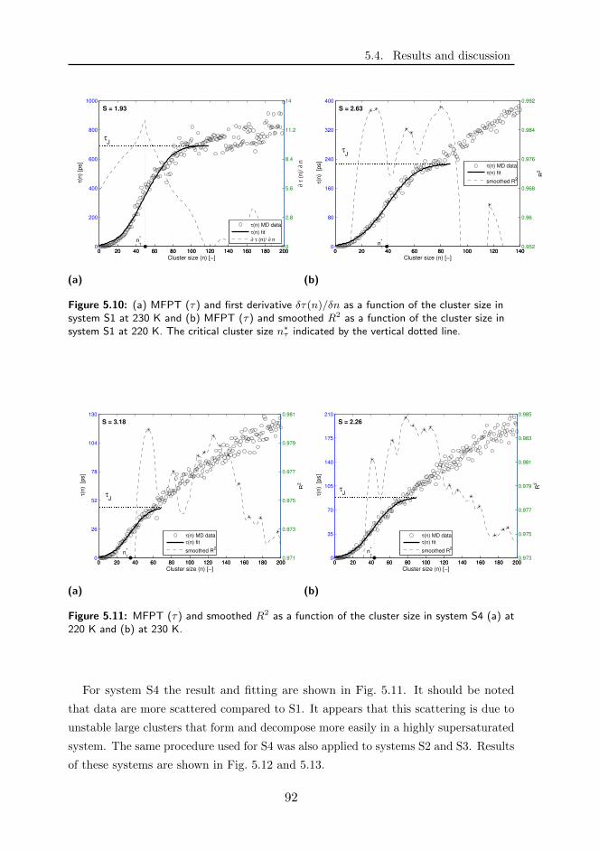
5.4. Results and discussion
0 20 40 60 80 100 120 140 160 180 2000
200
400
600
800
1000
Cluster size (n) [−]
τ(n
) [p
s]
τJ
0 20 40 60 80 100 120 140 160 180 2000
2.8
5.6
8.4
11.2
14
∂ τ
(n)/
∂ n
n*
τ
τ(n) MD data
τ(n) fit
∂ τ (n)/ ∂ n
S = 1.93
(a)
0 20 40 60 80 100 120 1400
80
160
240
320
400
Cluster size (n) [−]
τ(n
) [ps]
τJ
n*
τ
0 20 40 60 80 100 120 1400.952
0.96
0.968
0.976
0.984
0.992
R2
τ(n) MD data
τ(n) fit
smoothed R2
S = 2.63
(b)
Figure 5.10: (a) MFPT (τ) and first derivative δτ(n)/δn as a function of the cluster size insystem S1 at 230 K and (b) MFPT (τ) and smoothed R2 as a function of the cluster size insystem S1 at 220 K. The critical cluster size n∗
τ indicated by the vertical dotted line.
0 20 40 60 80 100 120 140 160 180 2000
26
52
78
104
130
Cluster size (n) [−]
τ(n
) [
ps]
τJ
n*
τ
0 20 40 60 80 100 120 140 160 180 2000.971
0.973
0.975
0.977
0.979
0.981
R2
τ(n) MD data
τ(n) fit
smoothed R2
S = 3.18
(a)
0 20 40 60 80 100 120 140 160 180 2000
35
70
105
140
175
210
Cluster size (n) [−]
τ(n
) [
ps]
τJ
n*
τ
0 20 40 60 80 100 120 140 160 180 2000.973
0.975
0.977
0.979
0.981
0.983
0.985
R2
τ(n) MD data
τ(n) fit
smoothed R2
S = 2.26
(b)
Figure 5.11: MFPT (τ) and smoothed R2 as a function of the cluster size in system S4 (a) at220 K and (b) at 230 K.
For system S4 the result and fitting are shown in Fig. 5.11. It should be noted
that data are more scattered compared to S1. It appears that this scattering is due to
unstable large clusters that form and decompose more easily in a highly supersaturated
system. The same procedure used for S4 was also applied to systems S2 and S3. Results
of these systems are shown in Fig. 5.12 and 5.13.
92

Chapter 5. Carbon dioxide nucleation in methane
0 20 40 60 80 100 120 140 160 180 2000
40
80
120
160
200
Cluster size (n) [−]
τ(n
) [
ps]
τJ
n*
τ
0 20 40 60 80 100 120 140 160 180 2000.95
0.9572
0.9644
0.9716
0.9788
0.986
R2
τ(n) MD data
τ(n) fit
smoothed R2
S = 2.93
(a)
0 20 40 60 80 100 120 140 160 180 2000
74
148
222
296
370
Cluster size (n) [−]
τ(n
) [
ps]
τJ
n*
τ
0 20 40 60 80 100 120 140 160 180 2000.93
0.942
0.954
0.966
0.978
0.99
R2
τ(n) MD data
τ(n) fit
smoothed R2
S = 2.15
(b)
Figure 5.12: MFPT (τ) and smoothed R2 as a function of the cluster size in system S2 (a) at220 K and (b) at 230 K.
0 20 40 60 80 100 120 140 160 1800
28
56
84
112
140
Cluster size (n) [−]
τ(n
) [
ps]
τJ
n*
τ
0 20 40 60 80 100 120 140 160 1800.972
0.975
0.978
0.981
0.984
0.987
R2
τ(n) MD data
τ(n) fit
smoothed R2
S = 3.06
(a)
0 50 100 150 200 250 3000
70
140
210
280
350
Cluster size (n) [−]
τ(n
) [
ps]
τJ
n*
τ
0 50 100 150 200 250 3000.982
0.9832
0.9844
0.9856
0.9868
0.988
R2
τ(n) MD data
τ(n) fit
smoothed R2
S = 2.22
(b)
Figure 5.13: MFPT (τ) and smoothed R2 as a function of the cluster size in system S3 (a) at220 K and (b) at 230 K.
93

5.4. Results and discussion
Table
5.2:
Sim
ulatio
nresu
ltsan
dth
eoreticalp
redictio
no
fn
ucleatio
nrates
(J)
in1026
cm−3s −
1an
dcritical
cluster
sizeo
fC
O2
at2
20
Kan
d2
30
K.
No
tation
sare
asfo
llows:S
isth
esu
persatu
ration
ratio,
n∗
the
criticalclu
stersize
wh
ilesu
bscrip
tsrepresen
tth
em
etho
do
fco
mp
utatio
n.
System
at
220
Kat
230
K
SJYM
JM
FPT
n∗M
FPT
JCNT
n∗CNT
SJYM
JM
FPT
n∗M
FPT
JCNT
n∗CNT
S1
2.6
332.7±
2.9
9.1±
1.9
39
4.7
20
1.9
33.2±
1.6
3.0±
1.0
50
0.4
37
S1†
2.6
629.6±
2.1
12.3±
4.3
33
6.1
19
1.9
33.6±
0.9
3.4±
2.6
46
0.4
37
S2
2.9
3236.5±
5.7
30.2±
6.3
38
35.9
15
2.1
549.0±
5.7
19.4±
5.9
40
12.2
24
S3
3.0
6394.0±
16.2
53.9±
11.7
33
71.5
13
2.2
2135.2±
5.5
19.8±
4.1
55
26.8
21
S4
3.1
8605.4±
55.1
75.0±
16.2
35
123.1
12
2.2
6219.0±
12.8
38.7±
10.2
43
43.4
19
†Sam
esy
stemS1,
but
for
which
equilib
ratio
nw
as
perfo
rmed
at
350
K.
94

Chapter 5. Carbon dioxide nucleation in methane
5.4.3 Comparison of nucleation rates
The nucleation rates obtained from these two methods on all systems are summarized
in Table 5.2. The values of the nucleation rates range from 1026 to 1028 cm−3s−1. The
threshold method is denoted as YM. It is clear from the Table that the nucleation
rates predicted by the threshold method are one order of magnitude larger than those
predicted by the MFPT method. This is in agreement with the results of Chapter 4
for water nucleation. The only exception is system S1 at mild quenching (230 K),
where both the YM and MFPT methods predict J ≈ 3× 1026 cm−3s−1. The effect of
the equilibrium temperature before quenching was also investigated. System S1 was
also equilibrated at 350 K instead of 530 K. These results are indicated under S1† in
Table 5.2. It is clear that a lower starting temperature did not seriously affect the
nucleation process.
Supersaturations (S) and theoretical predictions of the CNT nucleation rates are
also given in Table 5.2. The equilibrium parameters were taken from the Span and
Wagner EOS. Uncertainties were computed as described in Chapter 4.
The results presented in Table 5.2 show that supersaturation and nucleation rates
increased with increasing densities. Moreover, these systems showed highly scattered
data for the MFPT method. With increasing CO2 density, and thus supersaturation,
the YM method was easier to apply as the linear regime in the growth curves became
more pronounced. On the other hand, the estimation of τJ in the MFPT method
became more cumbersome. Still, Table 5.2 shows that the uncertainties arising from
the application of the YM method were typically below 12%, which are in the same
range as for the water systems in our previous studies. However, for supersaturations
below 2, the uncertainties for both methods were larger than 20%.
5.4.4 Comparison with CNT and literature
In Fig. 5.14 all nucleation rates from the present work are shown as a function
of supersaturation. The CNT predictions and the results of Horsch et al. 59 are also
shown. The latter represent canonical ensemble simulations of pure CO2 nucleation.
Their nucleation simulations were performed at 228 K and the nucleation rates were
obtained from the threshold method. Here the result computed from their threshold of
50 is shown.
As already shown in Table 5.2, our YM predictions are within one order of magnitude
from the CNT predictions. MFPT showed fairly good agreement with CNT for the
nucleation rates, while for the critical cluster size the CNT predictions were typically
95
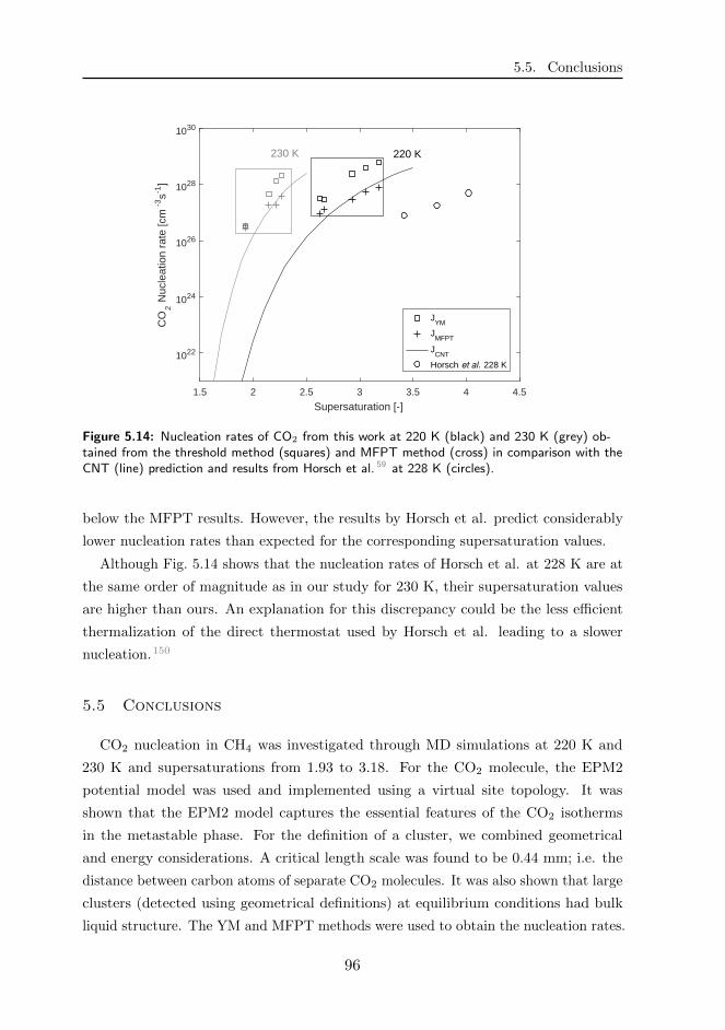
5.5. Conclusions
1.5 2 2.5 3 3.5 4 4.5
Supersaturation [-]
1022
1024
1026
1028
1030
CO
2 N
ucle
atio
n ra
te [c
m-3
s-1]
220 K230 K
JYM
JMFPT
JCNT
Horsch et al. 228 K
Figure 5.14: Nucleation rates of CO2 from this work at 220 K (black) and 230 K (grey) ob-tained from the threshold method (squares) and MFPT method (cross) in comparison with theCNT (line) prediction and results from Horsch et al. 59 at 228 K (circles).
below the MFPT results. However, the results by Horsch et al. predict considerably
lower nucleation rates than expected for the corresponding supersaturation values.
Although Fig. 5.14 shows that the nucleation rates of Horsch et al. at 228 K are at
the same order of magnitude as in our study for 230 K, their supersaturation values
are higher than ours. An explanation for this discrepancy could be the less efficient
thermalization of the direct thermostat used by Horsch et al. leading to a slower
nucleation.150
5.5 Conclusions
CO2 nucleation in CH4 was investigated through MD simulations at 220 K and
230 K and supersaturations from 1.93 to 3.18. For the CO2 molecule, the EPM2
potential model was used and implemented using a virtual site topology. It was
shown that the EPM2 model captures the essential features of the CO2 isotherms
in the metastable phase. For the definition of a cluster, we combined geometrical
and energy considerations. A critical length scale was found to be 0.44 mm; i.e. the
distance between carbon atoms of separate CO2 molecules. It was also shown that large
clusters (detected using geometrical definitions) at equilibrium conditions had bulk
liquid structure. The YM and MFPT methods were used to obtain the nucleation rates.
96
Chapter 5. Carbon dioxide nucleation in methane
The nucleation rates predicted by the threshold method were one order of magnitude
larger than those predicted by the MFPT method. The CNT predictions showed
agreement with the nucleation rates from the MFPT method. The CNT predictions
for the critical cluster size were typically below those predicted by the MFPT method.
The nucleation rates obtained from the YM method of Horsch et al. 59 at 228 K were
on the same order of magnitude (1027 − 1028 cm−3s−1) as our YM results at 230 K.
However, their supersaturation values were much higher than ours, possibly due to less
efficient thermalization of direct thermostatting. We showed that CO2 nucleation in
methane can be induced at relatively low supersaturations. but that high densities
were needed.
97

5.5. Conclusions
98

6Conclusions
This thesis research investigated the nucleation of water and carbon dioxide by
performing molecular dynamics simulations with the purpose of assessing the validity
of a single impurity phase separation step as part of the pre-treatment of natural gas
prior to liquefaction.
The nucleation behavior of water in argon carrier gas was first investigated. For
this binary system, comprised of 5000 molecules of condensing vapor, the effect of two
different model potentials on the homogeneous nucleation rates at T = 350 K was
studied. The two water models used were the TIP4P model and the re-parametrization
of the TIP4P; the TIP4P/2005 model, which was chosen due to its excellent predictions
of the phase diagram of water. Nucleation was triggered by a rapid quenching from 1000
K to 350 K. It was found that the stability of any cluster, even if large, strongly depended
on the energetic interactions with its surrounding molecules. By carefully tracing the
consistency of the largest surviving cluster, we observed that over time almost all
of the initial molecules gradually evaporated. Thus, the molecular composition of
a large stable cluster considerably changes throughout the nucleation phase. The
MD nucleation rates were derived following the threshold method or Yasuoka and
Matsumoto (YM) method. The nucleation rate for TIP4P was found to be 1.08× 1027
cm−3s−1. Remarkably, our result is very close to that of Yasuoka & Matsumoto 156 ,
in spite of the fact that they used different parameters for the cluster definition and
different values for the cutoff radius. Furthermore, it was found that the TIP4P/2005
99

model prescribes faster dynamics, leading to a nucleation rate of 2.30× 1027 cm−3s−1,
which is two times larger than TIP4P. In addition, it also led to the formation of a
larger number of clusters. The uncertainty range of our results from six simulation
runs for each case show a high degree of accuracy (up to 9%). This accuracy is
significantly higher than the water nucleation rates generated in large scale (million
particle) simulations with accuracies up to 34% at 350 K.5
The water vapor supersaturation ratios, S, were 7.57 for the TIP4P potential
and 48.65 for the TIP4P/2005 potential. CNT prediction for the nucleation rate of
TIP4P was approximately one order of magnitude lower than the prediction of the
TIP4P/2005 model. CNT overestimated the TIP4P nucleation rates by half an order
of magnitude. The discrepancy was larger for TIP4P/2005, which we attributed to the
vapor description of the water model.
Our data were compared with predictions from literature in a scaled plot. We
found that our results complemented existing data for high supersaturation and high
nucleation rates. At the same time, our results were consistent with data from
Tanaka,130 Angelil5 and Perez.116
The influence of the molecular properties and concentration of different carrier gases
on water nucleation at 350 K was also investigated. For these systems the TIP4P/2005
model was used to represent water molecules and the LJ potential for helium, methane,
and argon molecules. To generate nucleation rate results, the mean first passage time
(MFPT) and YM methods were used. The MFPT results were found to be typically
one order of magnitude lower than the YM method for all carrier gases. This finding is
in agreement with earlier results from literature.
Surprisingly, it was found that the nucleation rates of water in the three carrier
gases did not show large differences, although those for methane were found to be
systematically higher. We found that these small differences were clearly correlated
with the amount of removed latent heat and with the water-carrier gas and carrier
gas-carrier gas molecular collisions. Methane led to the highest nucleation rate, thus
showing that thermalization is not governed by the molecular mass of the carrier gas.
For heavier carrier gases, the number of collisions increased and the heat removal
decreased, which resulted in lower nucleation rates. Mass effects were systematically
studied. From the cluster distribution in these simulations it was found that more
water monomers and smaller water nuclei were found in a heavier carrier gas than in a
lighter carrier gas. Moreover, for identical masses, the different interaction parameters
of the carrier gases led to discrepancies in thermalization efficiency. This finding shows
that interaction parameters also play a role in thermalization.
100

Chapter 6. Conclusions
The concentration effect of the carrier gas was also studied. Upon increasing the
background concentration of the carrier gases, both the thermalization efficiency and
nucleation rates increased. Furthermore, for a doubled carrier gas concentration the
nucleation rates increased by a factor of 1.3, slightly less than in literature results.161
For tripled carrier gas concentration the nucleation rates increased by almost a factor
of two.
Preliminary results on water nucleation in methane and carbon dioxide were also
presented. Carbon dioxide was added in concentrations of 9% and 23% to these systems.
It was observed that very few CO2 molecules were trapped within the water cluster,
but only temporarily. Thus, they were not considered part of a nucleating cluster. For
9% CO2 concentration the differences in nucleation rates were negligible. However, for
the 23% concentration of CO2 nucleation rates increased notably. Moreover, the effect
of CO2 was stronger at higher supersaturation. A qualitative comparison of our results
for 23% of added CO2 with experimental results of Holten using 25% CO2,57 showed
that nucleation rates increased within the same order of magnitude.
CO2 nucleation in CH4 was investigated at 220 K and 230 K in supersaturation ranges
from 1.93 to 3.18. Although the systems exhibited relatively low supersaturations, the
high density (75 up to 125 mg cm−3) of the nucleating phase induced instability in the
cluster formation. For the CO2 molecule, the EPM2 potential model was implemented
using a virtual site topology. It was shown that the EPM2 model captures the essential
features of the CO2 isotherms in the metastable phase prescribed by the PR EOS. It
was also shown that large sized clusters at equilibrium conditions could be considered
bulk liquid at the corresponding temperature. By combining energy and geometrical
considerations, we found that a critical length of 0.44 nm was sufficient to define the
liquid phase. The YM and MFPT methods were used to obtain the nucleation rates.
As also seen in Chapter 4, the nucleation rates predicted by the threshold method were
one order of magnitude larger than those predicted by the MFPT method. The CNT
predictions showed agreement with the nucleation rates from the MFPT method, and
YM predictions were within one order of magnitude from the CNT predictions. The
CNT predictions for the critical cluster size were typically below those predicted by the
MFPT method. The nucleation rates obtained from the YM method of Horsch et al. 59
at 228 K were approximately in the same order of magnitude (1027 − 1028 cm−3s−1)
as our YM results at 230 K. However, their supersaturation values were much higher
than ours, possibly due to less efficient thermalization of direct thermostatting.
101

102

AA.1 Liquid structure
Cluster definitions for a polyatomic linear molecule, like CO2, have already been
reported in literature.60,59,74 One example is given in Horsch et al. 60 in which the
geometrical criterion128 with respect to the center of mass rg = 3σ2 + L
4 (with σ the
LJ size parameter and L the length of the molecule) is used in combination with an
energetic single-molecule criterion and a graph criterion for which liquid clusters are
defined as the bi-connected components of the graph with the molecules as its nodes
and edges between the molecules that fulfil the pair criterion.
In this work, the first step was to verify the ability of a geometrical criterion to
capture the structure of the bulk liquid. As a reference point in the phase diagram for
the liquid CO2, we used the saturated liquid density at 230 K of 1128.7 mg cm−3 of
Span and Wagner’s EOS.127
103

A.1. Liquid structure
0.5 1 1.5 2 2.5 30
5
10
15
20
25
30
r [nm]
Lo
ca
l n
um
be
r d
en
sity [
nm
−3]
maximum cluster
maximum cluster
bulk
(a)
6 10 20 30 60 100 200 1000
0
2
4
6
8
10
using
6 10 20 30 60 100 200 300 1000
0
2
4
6
8
10
using
Cluster size [−]
Nu
mb
er
of
clu
ste
rs [−
]
maximumcluster
(b)
Figure A.1: (a) Local number density as function of distance for bulk CO2 at 230 K andmaximum clusters in sytem S2 at 1 ns after the quenching at 230 K using different geometricdefinitions. (b) Cluster distribution of the same S2 system. Top figure uses rlongS and thebottom fig rshortS as geometrical criterion to identify clusters.
Fig A.1a shows the local number density of the reference CO2 liquid as a function
of distance, which is denoted as bulk in the legend. The local density is defined as the
average number density of the system multiplied by the RDF between carbon atoms,
ρB · gCC(r). In this figure, zero corresponds to the center of the simulation box and
the maximum r distance is around half of the box size. The density value towards
which the RDF profile of the bulk converges (15.448 nm−3) corresponds to the 1128
mg cm−3 liquid density from the EOS prediction.127 From this bulk RDF the first
minimum was established at 0.575 nm(∼2σC), which we denote as rlongS . We thus used
this value and a smaller value of 0.44 nm (∼1.6σC) in the range of a typical LJ fluid
radius, which we call rshortS , with the aim of observing the effect of these radii on the
cluster structure and size estimation.
Fig. A.1b shows the cluster size distribution using these two radii for system S2 at
230 K. From this figure it is clear that using rlongS resulted in the detection of a greater
number of clusters and clusters of a larger size, which, unsurprisingly, is due to larger
interatomic distances. From each distribution the largest cluster was detected and the
local density was computed. These local densities of the maximum clusters for both
radii are shown in Fig. A.1a. It can be seen that the density of the clusters overlap at
the core and diverge at large distances from the bulk. The divergence clearly reflects
104

Appendix A.
the difference between the bulk and the cluster boundary properties. The profiles of
both maximum clusters follow the peaks of the bulk, but the values are positioned well
below the bulk density profile. This finding indicates that the detected clusters did not
reach the bulk liquid density at the core of the clusters.
To further investigate if the clusters can reach the bulk structure, the configurations
of the largest clusters from Fig. A.1a were used in a 100 ps long NVT simulation
performed at 230 K. Fig. A.2 compares the local density results of the equilibrated
maximum clusters with the bulk. In this figure it is clearly visible that the profile
of both clusters and bulk overlap at the first peak, indicating that stable clusters or
clusters in equilibrium did approach the bulk liquid structure. We thus conclude that
both definitions led to a correct liquid representation at the core of the cluster.
0.5 1 1.5 2 2.5 30
5
10
15
20
25
30
r [nm]
Lo
ca
l n
um
ber
de
nsity [n
m−
3]
maximum cluster
maximum cluster
bulk
Figure A.2: Local number density as a function of distance for bulk CO2 at 230 K and for thetwo equilibrated (at 230 K) maximum clusters using different geometric definitions.
A.2 Cluster size detection
Since the CO2 molecule is linear, the orientation of the molecules can generate
different size predictions of unstable clusters depending on the arrangements of molecules
in the identified clusters. To enhance detection of stable sized clusters, an additional
criterion, such as an energetic criterion, is usually applied.74 In this research, we
followed the energy criterion used by Horsch et al. 60 This assumes that when for a
single molecule i the expression mv2i +
∑i 6=j u(rij) < 0 (where m is the mass of the
molecule and vi the translational velocity of the molecule’s center of mass) holds, the
105

A.2. Cluster size detection
molecule is counted as a part of the liquid cluster. Thus, we considered the geometrical
definitions rlongS and rshortS in combination with the single-molecule energy criterion to
compare the largest cluster evolutions in system S1.
To obtain the cluster evolution, at each time step the largest cluster is identified and
the number of molecules is counted. This procedure was repeated and the averaged
values were taken over all simulation runs. The results are shown in Fig. A.3a. As one
would expect, there was a clear decrease in the size of the largest cluster evolution when
the intermolecular distance from rlongS (represented by stars) to rshortS (represented by
squares) was reduced. With the addition of the energy criterion to rshortS , the cluster
definition became two-fold restrictive, and thus discarded even more molecules (due
to the low cut-off distance). Note that the addition of the energy criterion for rlongS
reduced the cluster size at the same level as the rshortS definition. This finding shows
that the use of rshortS definition was sufficient to detect the actual size of CO2 clusters.
Thus, we concluded that the rshortS definition could be used in the research for cluster
detection.
0 100 200 300 400 500 600 700 800 900 10000
100
200
300
400
500
600
700
800
Num
ber
of m
ole
cule
s in the m
axim
um
clu
ste
r [−
]
Time [ps]
rS
long
rS
short
rS
long + energy
rS
short + energy
(a)
0 100 200 300 400 500 600 700 800 900 10000
100
200
300
400
500
600
700
800
Num
ber
of m
ole
cule
s in the m
axim
um
clu
ste
r [−
]
Time [ps]
rS
long
rS
short
rS
long & rot+trans en
rS
short & rot+trans en
(b)
Figure A.3: Comparison of the largest cluster evolution when using only geometric definitionswith using an additional energetic criterion that includes: (a) translational velocity or (b) trans-lational and rotational velocity.
However, to have a full picture of the energetic criterion, we included the rotational
velocity of the center of mass to the single-molecule energy criterion. In Fig. A.3b a
considerable reduction in the cluster size evolution due to the energy criterion can be
observed. It can also be noted that this reduction occurred to a similar extent for both
radii definitions.
106

Acknowledgments
Undertaking this PhD has been a challenging and truly life-changing experience
to me, with many ups and downs throughout the six year journey. There were times
in my PhD life when I thought to myself I cannot continue anymore, but in the
end I persevered and I am grateful to myself for it, because here I am, writing the
acknowledgments of my thesis!
I would like to express my gratitude towards my supervisor David Smeulders for
bearing with me on this journey. I know it was more of a bumpy road, but in the end
we have succeeded in aligning our way of working. Thank you for taking charge of
the project and helping me to find my way through this research field. Initially, you
were leaning towards an experimental approach for which you offered support, but as
a non-experimentalist, I was afraid I will blow up the lab one day. In the end, the
numerical approach has prevailed and I am happy you allowed it to materialize.
Many thanks go to my advisor Silvia Gaastra-Nedea, who has been both a moral
support and great guidance into the subject of molecular dynamics. You always made
me feel like home through you empathy and by sharing the same mother tongue. I am
grateful for all the support you gave me even when you had limited amount of time
designated for work in the last years.
I greatly appreciate the opportunity given to me by my supervisor Jacques Dam, to
interview for this PhD project. I would like to thank you for your always so friendly
emails and for your prompt replies at any hour of the day or night.
During the term of this project other people from outside this project offered much
needed technical support. I am grateful to Henk Huinink who has contributed to the
work in Chapter 4. Also, a great thanks to Moritz Wolf, who has taken from his time
and offered support on Chapter 5. Thank you Jan Hasker, for always troubleshooting
the software errors I was encountering and guiding me through solving them even if
that involved the scary thought of updating Ubuntu. A big thanks goes to Bobby, who
has guided me in the use of GROMACS. Foremost, I would like to thank Duncan for
being the support I very much needed in the last year of my PhD. I highly value you
as a teacher, you have thought me a lot about writing and I am grateful I had the
opportunity to collaborate with you through this project. I will definitely miss the
encouragement you always expressed in your emails and your 'always there' availability.
107
This journey would have not been complete without sharing it with my dear
colleagues who have made my stay in TU/e easier and full fun moments. I would
like to thank all colleagues that I had the chance to meet during my PhD life. To
start, I will always remember the pleasant coffee breaks of my first years with Eldhose,
JungHan, Gokalp, Esubalew, Shuiquan when they were telling me to enjoy the honey
moon phase of my PhD. I want to thank him for his companionship to Manoj, with
whom I shared great memories from the squash lessons or from trying to learn the
language of the dutch in the classes offered by TU/e. Also I would like to thank Jaap,
Giel and Coen for the deep conversations and the kind advice they offered. I want to
thank my office mate Ruud for the 'talk therapy sessions' we sometimes had, you were
of great support to me and cheered me up on my bad days. Thank you for bringing the
coffee breaks and/or outings in the Energy Technology group to Max, Luca, Mauro,
Koen, Patty, Mohammadreza, Taha, Shravan, Amar. Last but not least, I would like
to thank Linda and Marjan for taking care of the appointments with David and for all
the help they gave me.
My deep appreciation goes to all the friends I met in the Netherlands and encouraged
me in this journey. Thank you for always believing in me and supporting me to my
good friends Mihaela, Irina and Alexandra. I am also grateful to have met and shared
moments of my PhD with Lisa, Monica, Vidit, Franz, Serhat, Joshua, Michael. For
brightening my life by means of music, I am grateful to Waldo with whom I shared so
many wonderful gigs. I want to thank Music with Strangers for existing, I will never
forget the great Popei concerts we had.
A very special thank you goes to Alex, who has been by my side for the most part
of this PhD and lived through me the life of a PhD. I will always be grateful for the
help you have given me.
I am also indebted to my relatives and friends back in Romania. I am grateful to the
trust and support to my aunt Carmen, my uncle Lucian, to my aunt Tusi, my cousin
Alice and my aunt Violeta, and to my close friends Alina, Deya, Gabi, Andrada, Paul.
A heartful thank you goes to my dear parents who have always believed in me and
encouraged me to do what was best for myself, without putting too much pressure. I
am especially grateful to my mom for her excessive nurturing way of being and for her
continuous desire to feed me. I love you both the most!
108

Curriculum Vitae
Lucia Raluca Dumitrescu was born on November
3rd 1988 in the town of Lipova (Arad county), Romania.
She graduated in Mathematics and Computer Science
in 2007 from Elena Ghiba Birta National College in
Arad, Romania. In 2010, she graduated with a Bach-
elor's degree in Mathematics and Computer Science
from the Aurel Vlaicu University of Arad. Thereafter,
she opted to follow a double degree Master's in Indus-
trial and Applied Mathematics, in which in the first
year she studied in Romania at the West University of
Timisoara and in the second year in The Netherlands
at the Eindhoven University of Technology. In 2012,
she graduated with a master’s degree and applied for a
PhD position in the Energy Technology group of Prof.
David Smeulders at Eindhoven University of Technology. In 2013, she started the PhD
project, the results of which are presented in this work. Since 2019, she has worked as
a design engineer in the metrology department of ASML.
109

110

References
[1] Abascal, J. L. F. & Vega, C. (2005). A general purpose model for the condensed
phases of water: TIP4P/2005. The Journal of Chemical Physics, 123(23).
[2] Alder, B. J. & Wainwright, T. E. (1957). Phase Transition for a Hard Sphere
System. Citation: J. Chem. Phys, 27, 1208.
[3] Alejandre, J., Tildesley, D. J., & Chapela, G. A. (1995). Molecular dynamics
simulation of the orthobaric densities and surface tension of water. The Journal
of Chemical Physics, 102(11), 4574–4583.
[4] Allen, M. P. & Tildesley, D. J. (1989). Computer Simulation of Liquids. New
York, NY, USA: Clarendon Press.
[5] Angelil, R., Diemand, J., Tanaka, K. K., & Tanaka, H. (2015). Homogeneous
SPC/E water nucleation in large molecular dynamics simulations. The Journal
of Chemical Physics, 143(6), 064507.
[6] Anisimov, M. P., Hopke, P. K., Shandakov, S. D., & Shvets, I. I. (2000). n-
pentanol-helium homogeneous nucleation rates. The Journal of Chemical Physics,
113(5), 1971–1975.
[7] Aragones, J. L., Conde, M. M., Noya, E. G., & 20, C. (2009). The phase diagram
of water at high pressures as obtained by computer simulations of the TIP4P/2005
model: the appearance of a plastic crystal phase. Phys. Chem. Chem. Phys., 11,
543–555.
[8] Ares, S., Voulgarakis, N. K., Rasmussen, K. O., & Bishop, A. R. (2005). Bubble
Nucleation and Cooperativity in DNA Melting. Phys. Rev. Lett., 94, 035504.
[9] Avendano, C., Lafitte, T., Galindo, A., Adjiman, C. S., Jackson, G., & Muller,
E. A. (2011). SAFT-γ Force Field for the Simulation of Molecular Fluids. 1. A
Single-Site Coarse Grained Model of Carbon Dioxide. The Journal of Physical
Chemistry B, 115(38), 11154–11169.
[10] Bartell, L. S. & Wu, D. T. (2006). A new procedure for analyzing the nucleation
kinetics of freezing in computer simulation. The Journal of Chemical Physics,
125(19), 194503.
111

[11] Becker, R. & Doring, W. (1935). Kinetische behandlung der keimbildung in
ubersattigten dampfen. Annalen der Physik, 416(8), 719–752.
[12] Berendsen, H. J. C., Postma, J. P. M., van Gunsteren, W. F., DiNola, A., &
Haak, J. R. (1984). Molecular dynamics with coupling to an external bath. The
Journal of Chemical Physics, 81(8), 3684–3690.
[13] Blander, M. (1979). Bubble nucleation in liquid. Adv. Colloid Interface Sci., 10,
1–32.
[14] Blander, M. & Katz, J. L. (1972). The thermodynamics of cluster formation in
nucleation theory. Journal of Statistical Physics, 4(1), 55–59.
[15] Brooks, B. R., Brooks, C. L., Mackerell, A. D., Nilsson, L., Petrella, R. J., Roux,
B., Won, Y., Archontis, G., Bartels, C., Boresch, S., Caflisch, A., Caves, L.,
Cui, Q., Dinner, A. R., Feig, M., Fischer, S., Gao, J., Hodoscek, M., Im, W.,
Kuczera, K., Lazaridis, T., Ma, J., Ovchinnikov, V., Paci, E., Pastor, R. W.,
Post, C. B., Pu, J. Z., Schaefer, M., Tidor, B., Venable, R. M., Woodcock, H. L.,
Wu, X., Yang, W., York, D. M., Karplus, M., York, D., & Karplus, M. (2009).
CHARMM: the biomolecular simulation program. Journal of computational
chemistry, 30(10), 1545–614.
[16] Brus, D., Zdımal, V., & Smolık, J. (2008). Homogeneous nucleation rate mea-
surements in supersaturated water vapor. The Journal of Chemical Physics,
129(17).
[17] Brus, D., Zdımal, V., & Stratmann, F. (2006). Homogeneous nucleation rate
measurements of 1-propanol in helium: The effect of carrier gas pressure. The
Journal of Chemical Physics, 124(16), 164306.
[18] Brus, D., Zdımal, V., & Uchtmann, H. (2009a). Homogeneous nucleation rate
measurements in supersaturated water vapor II. The Journal of Chemical Physics,
131(7), 074507.
[19] Brus, D., Zdımal, V., & Smolık, J. (2009b). Erratum: “Homogeneous nucleation
rate measurements in supersaturated water vapor” [J. Chem. Phys. 129, 174501
(2008)]. The Journal of Chemical Physics, 130(21), 219902.
[20] Bulacu, M. ., Goga, N. ., Zhao, W. ., Rossi, G. ., Monticelli, L. ., Periole, X. .,
& Marrink (2013). Improved Angle Potentials for Coarse-Grained Molecular
Dynamics Simulations. Journal of Chemical Theory and Computation, 9(8),
3282–3292.
112

[21] Burgers, W., Northrop, P., Kheshgi, H., & Valencia, J. (2011). Energy Procedia
Worldwide development potential for sour gas. Energy Procedia, 4, 2178–2184.
[22] Burgot, J.-L. (2017). The Configurational Partition Function: Molecular Distri-
bution Functions. In The Notion of Activity in Chemistry (pp. 319–327). Cham:
Springer International Publishing.
[23] Chkonia, G., Wolk, J., Strey, R., Wedekind, J., & Reguera, D. (2009). Evaluating
nucleation rates in direct simulations. The Journal of Chemical Physics, 130(6),
064505.
[24] Christen, M., Hunenberger, P. H., Bakowies, D., Baron, R., Burgi, R., Geerke,
D. P., Heinz, T. N., Kastenholz, M. A., Krautler, V., Oostenbrink, C., Peter,
C., Trzesniak, D., & van Gunsteren, W. F. (2005). The GROMOS software for
biomolecular simulation: GROMOS05. Journal of Computational Chemistry,
26(16), 1719–1751.
[25] Courtney, W. G. (1961). Remarks on homogeneous nucleation. The Journal of
Chemical Physics, 35(6), 2249–2250.
[26] Cygan, R. T., Romanov, V. N., & Myshakin, E. M. (2012). Molecular Simulation
of Carbon Dioxide Capture by Montmorillonite Using an Accurate and Flexible
Force Field. The Journal of Physical Chemistry C, 116(24), 13079–13091.
[27] Darden, T., York, D., & Pedersen, L. (1993). PARTICLE mesh Ewald: An
Nalog(N) method for Ewald sums in large systems. The Journal of Chemical
Physics, 98(12), 10089–10092.
[28] Dumitrescu, L. R., Smeulders, D. M. J., Dam, J. A. M., & Gaastra-Nedea, S. V.
(2017). Homogeneous nucleation of water in argon. Nucleation rate computation
from molecular simulations of TIP4P and TIP4P/2005 water model. The Journal
of Chemical Physics, 146(8), 084309.
[29] Ellerby, H. M. & Reiss, H. (1992). Toward a molecular theory of vapor-phase
nucleation. II. Fundamental treatment of the cluster distribution. The Journal
of Chemical Physics, 97(8), 5766–5772.
[30] Ewald, P. P. (1921). Die Berechnung optischer und elektrostatischer Gitterpo-
tentiale. Annalen der Physik, 369(3), 253–287.
[31] Farkas, L. (1927). Keimbildungsgeschwindigkeit in ubersattigten dampfen. Z.
Phys. Chem. (Leipzig), 125, 236.
113

[32] Feder, J., Russell, K., Lothe, J., & Pound, G. (1966). Homogeneous nucleation
and growth of droplets in vapours. Advances in Physics, 15(57), 111–178.
[33] Fladerer, A. & Strey, R. (2006). Homogeneous nucleation and droplet growth
in supersaturated argon vapor: The cryogenic nucleation pulse chamber. The
Journal of Chemical Physics, 124(16).
[34] Ford, I. J. & Clement, C. F. (1989). The effects of temperature fluctuations
in homogeneous nucleation theory. Journal of Physics A: Mathematical and
General, 22(18), 4007.
[35] Franck, J. P. & Hertz, H. G. (1956). Messung der kritischen Ubersattigung von
Dampfen mit der Diffusionsnebelkammer. Zeitschrift fur Physik, 143(5), 559–590.
[36] Fransen, M. A. L. J., Hruby, J., Smeulders, D. M. J., & van Dongen, M. E. H.
(2015). On the effect of pressure and carrier gas on homogeneous water nucleation.
The Journal of Chemical Physics, 142(16), 164307.
[37] Frenkel, D. & Smit, B. (2002). Understanding molecular simulation : from
algorithms to applications.
[38] Frenkel, J. (1939). A general theory of heterophase fluctuations and pretransition
phenomena. The Journal of Chemical Physics, 7(7), 538–547.
[39] Gavezzotti, A. (2007). Molecular aggregation: structure analysis and molecular
simulation of crystals and liquids. IUCr Monographs on crystallography. Oxford:
Oxford University Press.
[40] Gingrich, N. S. (1943). The Diffraction of X-Rays by Liquid Elements. Reviews
of Modern Physics, 15(1), 90–110.
[41] Girshick, S. L. (1991). Comment on: “Self-consistency correction to homogeneous
nucleation theory”. The Journal of Chemical Physics, 94(1), 826–827.
[42] Girshick, S. L. & Chiu, C. (1990). Kinetic nucleation theory: A new expression
for the rate of homogeneous nucleation from an ideal supersaturated vapor. The
Journal of Chemical Physics, 93(2), 1273–1277.
[43] Gonzalez, M. A. & Abascal, J. L. F. (2010). The shear viscosity of rigid water
models. The Journal of Chemical Physics, 132(9).
[44] Green, M. S. (1954). Markoff Random Processes and the Statistical Mechanics of
TimeaDependent Phenomena. II. Irreversible Processes in Fluids. The Journal
of Chemical Physics, 22(3), 398–413.
114

[45] Hale, B. N. (1986). Application of a scaled homogeneous nucleation-rate formalism
to experimental data at TTc. Phys. Rev. A, 33, 4156–4163.
[46] Hale, B. N. (1988). Scaled models for nucleation, (pp. 321–349). Springer Berlin
Heidelberg: Berlin, Heidelberg.
[47] Hale, B. N. (2004). Computer Simulations, Nucleation Rate Predictions and
Scaling. In M. Kasahara & M. Kulmala (Eds.), Proceedings of the 16th Interna-
tional Conference on Nucleation and Atmospheric Aerosols (pp. 3–13). Kyoto,
Japan: Kyoto University Press.
[48] Hale, B. N. & DiMattio, D. J. (2004). Scaling of the Nucleation Rate and a Monte
Carlo Discrete Sum Approach to Water Cluster Free Energies of Formation. The
Journal of Physical Chemistry B, 108(51), 19780–19785.
[49] Hanggi, P., Talkner, P., & Borkovec, M. (1990). Reaction-rate theory: fifty years
after Kramers. Rev. Mod. Phys., 62, 251–341.
[50] Harris, J. G. & Yung, K. H. (1995). Carbon Dioxide’s Liquid-Vapor Coexistence
Curve and Critical Properties As Predicted by a Simple Molecular Model. J.
Phys. Chem, 99, 12021–12024.
[51] Heist, R. H. & He, H. (1994). Review of vapor to liquid homogeneous nucleation
experiments from 1968 to 1992. Journal of Physical and Chemical Reference
Data, 23(5), 781.
[52] Helfand, E. (1960). Transport Coefficients from Dissipation in a Canonical
Ensemble. Phys. Rev., 119, 1–9.
[53] Hernandes, M. Z., Da Silva, J. B. P., & Longo, R. L. (2003). Chemometric study
of liquid water simulations. I. The parameters of the TIP4P model potential.
Journal of Computational Chemistry, 24(8), 973–981.
[54] Hess, B., Bekker, H., Berendsen, H. J. C., & Fraaije, J. G. E. M. (2005). LINCS:
A linear constraint solver for molecular simulations. Journal of Computational
Chemistry, 18(12), 1463–1472.
[55] Hess, B., Kutzner, C., van der Spoel, D., & Lindahl, E. (2008). GROMACS
4:a Algorithms for Highly Efficient, Load-Balanced, and Scalable Molecular
Simulation.
[56] Hockney, R., Goel, S., & Eastwood, J. (1974). Quiet high-resolution computer
models of a plasma. Journal of Computational Physics, 14(2), 148 – 158.
115

[57] Holten, V. (2009). Water nucleation : wave tube experiments and theoretical
considerations. PhD thesis, Department of Applied Physics.
[58] Holten, V., Labetski, D. G., & van Dongen, M. E. H. (2005). Homogeneous
nucleation of water between 200 and 240 K: New wave tube data and estimation
of the Tolman length. The Journal of Chemical Physics, 123(10), 104505.
[59] Horsch, M., Lin, Z., Windmann, T., Hasse, H., & Vrabec, J. (2011). The air
pressure effect on the homogeneous nucleation of carbon dioxide by molecular
simulation. Atmospheric Research, 101(3), 519–526.
[60] Horsch, M., Vrabec, J., Bernreuther, M., Grottel, S., Reina, G., Wix, A., Schaber,
K., & Hasse, H. (2008). Homogeneous nucleation in supersaturated vapors of
methane, ethane, and carbon dioxide predicted by brute force molecular dynamics.
The Journal of Chemical Physics, 128(16), 164510.
[61] Humphrey, W., Dalke, A., & Schulten, K. (1996). VMD: visual molecular
dynamics. Journal of molecular graphics, 14(1), 33–38.
[62] Ismail, A. E., Grest, G. S., & Stevens, M. J. (2006). Capillary waves at the
liquid-vapor interface and the surface tension of water. The Journal of Chemical
Physics, 125(1).
[63] Jorgensen, W. L., Chandrasekhar, J., Madura, J. D., Impey, R. W., & Klein,
M. L. (1983). Comparison of simple potential functions for simulating liquid
water. The Journal of Chemical Physics.
[64] Kalikmanov, V. (2013). Nucleation Theory. Lecture Notes in Physics. Springer
Netherlands.
[65] Kalikmanov, V. I. (2006). Mean-field kinetic nucleation theory. The Journal of
Chemical Physics, 124(12), 124505.
[66] Kalikmanov, V. I. (2015). Effective binary theory of multi-component nucleation.
The Journal of Chemical Physics, 142(12), 124111.
[67] Kalikmanov, V. I., Wolk, J., & Kraska, T. (2008). Argon nucleation: Bringing
together theory, simulations, and experiment. The Journal of Chemical Physics,
128(12).
[68] Kashchiev, D. (1982). On the relation between nucleation work, nucleus size,
and nucleation rate. The Journal of Chemical Physics, 76(10), 5098–5102.
[69] Kashchiev, D. (1996). Effect of carrier-gas pressure on nucleation. The Journal
of Chemical Physics, 104(21), 8671–8677.
116
[70] Kashchiev, D. (2000). Nucleation. Butterworth-Heinemann.
[71] Katz, J. L. & Donohue, M. D. (1979). A Kinetic Approach to Homogeneous
Nucleation Theory, (pp. 137–155). John Wiley Sons, Ltd.
[72] Katz, J. L. & Wiedersich, H. (1977). Nucleation theory without Maxwell Demons.
Journal of Colloid and Interface Science, 61(2), 351–355.
[73] Kharlamov, G. V. & Zhilkin, S. V. (2017). Molecular dynamics simulation of the
molecular diffusion in gases and liquids. Engineering Letters, 25(2), 222–227.
[74] Kido, A. & Nakanishi, K. (1999). Molecular dynamics study of nucleation in
supersaturated vapor of carbon dioxide. Fluid Phase Equilibria, 158160, 79–86.
[75] Kim, Y. J., Wyslouzil, B. E., Gerald, W., Wolk, J., & Strey, R. (2004). Isothermal
Nucleation Rates in Supersonic Nozzles and the Properties of Small Water
Clusters. The Journal of Physical Chemistry A, 108(20), 4365–4377.
[76] Klinkenbijl, J., Dillion, M., & Heyman, E. (1999). Gas pre-treatment and their
impact on liquefaction processes. Gas Processors Association, Tulsa, OK (US).
[77] Kruh, R. F. (1962). Diffraction Studies of the Structure of Liquids. Chemical
Reviews, 62(4), 319–346.
[78] Kubo, R. (1957). Statistical-Mechanical Theory of Irreversible Processes. I.
General Theory and Simple Applications to Magnetic and Conduction Problems.
Journal of the Physical Society of Japan, 12(6), 570–586.
[79] Kunz, O., Klimeck, R., Wagner, R., & Jaeschke, W. (2007). The GERG-2004
wide-range equation of state for natural gases and other mixtures. Dusseldorf:
VDI-Verlag.
[80] Laaksonen, A., Talanquer, V., & Oxtoby, D. W. (1995). Nucleation: Mea-
surements, theory, and atmospheric applications. Annual Review of Physical
Chemistry, 46(1), 489–524. PMID: 24341941.
[81] Labetski, D. G., Holten, V., & van Dongen, M. E. H. (2004). Comment on “The
nucleation behavior of supercooled water vapor in helium” [J. Chem. Phys. 117,
5647 (2002)]. The Journal of Chemical Physics, 120(13), 6314–6314.
[82] LAMMPS (1995). Sandia national laboratories, website available at:
http://lammps.sandia.gov.
117

[83] Landau, L. D., Pitaevskii, L. P., & Lifshits, E. M. (1980). Statistical Physics:
Transl. from the Russian by JB Sykes and MJ Kearsley. 3d Ed. Rev. and Enl.
Pergamon Press.
[84] Lemmon, E. W., Huber, M. L., & McLinden, M. O. (2013). NIST Standard Ref-
erence Database 23: Reference Fluid Thermodynamic and Transport Properties-
REFPROP, Version 9.1, National Institute of Standards and Technology.
[85] Lihavainen, H. & Viisanen, Y. (2001). A Laminar Flow Diffusion Chamber for
Homogeneous Nucleation Studies. The Journal of Physical Chemistry B, 105(47),
11619–11629.
[86] Luijten, C. C. M., Bosschaart, K. J., & van Dongen, M. E. H. (1997). High
pressure nucleation in water/nitrogen systems. The Journal of Chemical Physics,
106(19), 8116–8123.
[87] Maitland, G. C. (1981). Intermolecular forces: their origin and determination.
Number 3. Oxford University Press.
[88] Manka, A., Bergmann, D., Ghosh, D., Strey, R., & Wolk, J. (2007). Preliminary
Results on Homogeneous Nucleation of Water: A Novel Measurement Technique
using the Two-valve Expansion Chamber, (pp. 260–264). Springer Netherlands:
Dordrecht.
[89] Manka, A. A., Brus, D., Hyvarinen, A.-P., Lihavainen, H., Wolk, J., & Strey, R.
(2010). Homogeneous water nucleation in a laminar flow diffusion chamber. The
Journal of Chemical Physics, 132(24), 244505.
[90] Matsubara, H., Koishi, T., Ebisuzaki, T., & Yasuoka, K. (2007). Extended study
of molecular dynamics simulation of homogeneous vapor-liquid nucleation of
water. The Journal of Chemical Physics, 127(21).
[91] Matsumoto, M., Takaoka, Y., & Kataoka, Y. (1993). Liquid-vapor interface
of water-methanol mixture. I. Computer simulation. The Journal of Chemical
Physics, 98(2), 1464–1472.
[92] McQuarrie, D. (2000). Statistical Mechanics. University Science Books.
[93] Meier, K., Laesecke, A., & Kabelac, S. (2001). A Molecular Dynamics Simulation
Study of the Self-Diffusion Coefficient and Viscosity of the Lennard-Jones Fluid.
International Journal of Thermophysics, 22(1), 161–173.
118

[94] Merikanto, J., Vehkamaki, H., & Zapadinsky, E. (2004). Monte carlo simulations
of critical cluster sizes and nucleation rates of water. The Journal of Chemical
Physics, 121(2), 914–924.
[95] Merker, T., Engin, C., Vrabec, J., & Hasse, H. (2010). Molecular model for
carbon dioxide optimized to vapor-liquid equilibria. The Journal of Chemical
Physics, 132(23), 234512.
[96] Metropolis, N., Rosenbluth, A. W., Rosenbluth, M. N., Teller, A. H., & Teller, E.
(1953). Equation of state calculations by fast computing machines. The Journal
of Chemical Physics, 21(6), 1087–1092.
[97] Miller, R. C., Anderson, R. J., Kassner, J. L., & Hagen, D. E. (1983). Homoge-
neous nucleation rate measurements for water over a wide range of temperature
and nucleation rate. The Journal of Chemical Physics, 78(6), 3204–3211.
[98] Mognetti, B. M., Yelash, L., Virnau, P., Paul, W., Binder, K., Muller, M., &
MacDowell, L. G. (2008). Efficient prediction of thermodynamic properties of
quadrupolar fluids from simulation of a coarse-grained model: The case of carbon
dioxide. The Journal of Chemical Physics, 128(10), 104501.
[99] Mokshin, A. V. & Galimzyanov, B. N. (2012). Steady-state homogeneous
nucleation and growth of water droplets: Extended numerical treatment. The
Journal of Physical Chemistry B, 116(39), 11959–11967. PMID: 22957738.
[100] Moore, E. B. & Molinero, V. (2011). Structural transformation in supercooled
water controls the crystallization rate of ice. , 479(7374), 506–508.
[101] Morishita, T. (2000). Fluctuation formulas in molecular-dynamics simulations
with the weak coupling heat bath. The Journal of Chemical Physics, 113(8),
2976–2982.
[102] Moultos, O. A., Zhang, Y., Tsimpanogiannis, I. N., Economou, I. G., & Maginn,
E. J. (2016). System-size corrections for self-diffusion coefficients calculated from
molecular dynamics simulations: The case of CO2, n-alkanes, and poly(ethylene
glycol) dimethyl ethers. The Journal of Chemical Physics, 145(7), 074109.
[103] Murthy, C. S., Singer, K., & McDonald, I. R. (1981). Interaction site models for
carbon dioxide. Molecular Physics.
[104] Nedea, S. V., van Steenhoven, A. A., Markvoort, A. J., Spijker, P., & Giordano,
D. (2014). Gas-surface interactions using accommodation coefficients for a dilute
119
and a dense gas in a micro- or nanochannel: Heat flux predictions using combined
molecular dynamics and Monte Carlo techniques. Phys. Rev. E, 89, 053012.
[105] Nieto-Draghi, C., de Bruin, T., Perez-Pellitero, J., Bonet Avalos, J., & Mackie,
A. D. (2007). Thermodynamic and transport properties of carbon dioxide from
molecular simulation. The Journal of Chemical Physics, 126(6), 064509.
[106] Nocent, M., Bertocchi, L., Espitalier, F., Baron, M., & Couarraze, G. (2001).
Definition of a Solvent System for Spherical Crystallization of Salbutamol Sulfate
by Quasi-Emulsion Solvent Diffusion (QESD) Method. Journal of Pharmaceutical
Sciences, 90(10), 1620 – 1627.
[107] Nose, S. (1984). A unified formulation of the constant temperature molecular
dynamics methods. The Journal of Chemical Physics, 81(1), 511–519.
[108] Oakley, M. T. & Wheatley, R. J. (2009). Additive and nonadditive models of
vapor-liquid equilibrium in CO2 from first principles. The Journal of Chemical
Physics, 130(3), 034110.
[109] Oh, K. J. & Zeng, X. C. (2001). Effect of carrier-gas pressure on barrier to
nucleation: Monte Carlo simulation of water/nitrogen system. The Journal of
Chemical Physics, 114(6), 2681–2686.
[110] Papadopoulou, V., Eckersley, R. J., Balestra, C., Karapantsios, T. D., & Tang,
M.-X. (2013). A critical review of physiological bubble formation in hyperbaric
decompression. Advances in Colloid and Interface Science, 191-192, 22 – 30.
[111] Paris: Scienomics; 2013 (2013). MAPS, version 3.3.2, Scienomics SARL, Paris.
[112] Parrinello, M. & Rahman, A. (1981). Polymorphic transitions in single crystals: A
new molecular dynamics method. Journal of Applied Physics, 52(12), 7182–7190.
[113] Peeters, P., Gielis, J. J. H., & van Dongen, M. E. H. (2002). The nucleation
behavior of supercooled water vapor in helium. The Journal of Chemical Physics,
117(12), 5647–5653.
[114] Peeters, P., Hruby, J., & van Dongen, M. E. H. (2001). High pressure nucleation
experiments in binary and ternary mixtures. The Journal of Physical Chemistry
B, 105(47), 11763–11771.
[115] Peng, D.-Y. & Robinson, D. B. (1976). A new two-constant equation of state.
Industrial & Engineering Chemistry Fundamentals, 15(1), 59–64.
[116] Perez, A. & Rubio, A. (2011). A molecular dynamics study of water nucleation
using the TIP4P/2005 model. The Journal of Chemical Physics, 135(24), 244505.
120
[117] Persson, R. A. X. (2011). Gaussian charge polarizable interaction potential for
carbon dioxide. The Journal of Chemical Physics, 134(3), 034312.
[118] Pi, H. L., Aragones, J. L., Vega, C., Noya, E. G., Abascal, J. L., Gonzalez,
M. A., & McBride, C. (2009). Anomalies in water as obtained from computer
simulations of the TIP4P/2005 model: density maxima, and density, isothermal
compressibility and heat capacity minima. Molecular Physics, 107(4-6), 365–374.
[119] Plimpton, S. (1995). Fast Parallel Algorithms for Short-Range Molecular Dy-
namics. Journal of Computational Physics, 117(1), 1–19.
[120] Pruppacher, H. R. & Klett, J. D. (1997). Microphysics of clouds and precipitation.
Dordrecht: Kluwer Academic Publishers, 2nd rev. and enl. ed. edition.
[121] Reguera, D. & Reiss, H. (2004). Fusion of the Extended Modified Liquid Drop
Model for Nucleation and Dynamical Nucleation Theory. Physical Review Letters,
93(16), 165701.
[122] Romer, F. & Kraska, T. (2007). Homogeneous nucleation and growth in supersat-
urated zinc vapor investigated by molecular dynamics simulation. The Journal
of Chemical Physics, 127(23), 234509.
[123] Santra, M. & Bagchi, B. (2011). Crossover dynamics at large metastability in
gas-liquid nucleation. Physical Review E - Statistical, Nonlinear, and Soft Matter
Physics.
[124] Schmitt, J. L., Whitten, J., Adams, G. W., & Zalabsky, R. A. (1990). Binary
nucleation of ethanol and water. The Journal of Chemical Physics, 92(6), 3693–
3699.
[125] Schrodinger, LLC (2015). The PyMOL molecular graphics system, version 1.8.
[126] Senger, B., Schaaf, P., Corti, D. S., Bowles, R., Voegel, J.-C., & Reiss, H. (1999).
A molecular theory of the homogeneous nucleation rate. I. Formulation and
fundamental issues. The Journal of Chemical Physics, 110(13), 6421–6437.
[127] Span, R. & Wagner, W. (1996). A New Equation of State for Carbon Dioxide
Covering the Fluid Region from the TripleaPoint Temperature to 1100 K at
Pressures up to 800 MPa. Journal of Physical and Chemical Reference Data,
25(6), 1509–1596.
[128] Stillinger, F. H. (1963). Rigorous Basis of the Frenkel-Band Theory of Association
Equilibrium. The Journal of Chemical Physics, 38(7), 1486–1494.
121

[129] Stone, A. (1996). The theory of intermolecular forces. Oxford University Press.
[130] Tanaka, K. K., Kawano, A., & Tanaka, H. (2014). Molecular dynamics simulations
of the nucleation of water: Determining the sticking probability and formation
energy of a cluster. The Journal of Chemical Physics, 140(11), 114302.
[131] Taylor, R. S., Dang, L. X., , & Garrett, B. C. (1996). Molecular Dynamics
Simulations of the Liquid/Vapor Interface of SPC/E Water. The Journal of
Physical Chemistry, 100(28), 11720–11725.
[132] Toner, M., Cravalho, E. G., & Karel, M. (1990). Thermodynamics and kinetics of
intracellular ice formation during freezing of biological cells. Journal of Applied
Physics, 67(3), 1582–1593.
[133] Van Der Spoel, D., Lindahl, E., Hess, B., Groenhof, G., Mark, A. E., & Berendsen,
H. J. C. (2005). GROMACS: Fast, flexible, and free. Journal of Computational
Chemistry, 26(16), 1701–1718.
[134] van Tricht, J., Fredrikze, H., & van der Laan, J. (1984). Neutron diffraction
study of liquid carbon dioxide at two thermodynamic states. Molecular Physics,
52(1), 115–127.
[135] Vega, C., Abascal, J. L. F., & Nezbeda, I. (2006). Vapor-liquid equilibria from
the triple point up to the critical point for the new generation of TIP4P-like
models: TIP4P/Ew, TIP4P/2005, and TIP4P/ice. The Journal of Chemical
Physics, 125(3).
[136] Vega, C. & de Miguel, E. (2007). Surface tension of the most popular models
of water by using the test-area simulation method. The Journal of Chemical
Physics, 126(15).
[137] Vehkamaki, H. (2006). Classical nucleation theory in multicomponent systems.
Springer Science & Business Media.
[138] Viisanen, Y., Strey, R., & Reiss, H. (1993). Homogeneous nucleation rates for
water. The Journal of Chemical Physics, 99(6), 4680–4692.
[139] Volmer, M. & Weber, A. (1926). Z. Physikal. Chemie, 119, 277–301.
[140] Vrabec, J., Stoll, J., & Hasse, H. (2001). A Set of Molecular Models for Symmetric
Quadrupolar Fluids. The Journal of Physical Chemistry B, 105(48), 12126–12133.
[141] Zdımal, V. & Smolık, J. (1998). Homogeneous nucleation rate measurements in
1-pentanol vapor with helium as a buffer gas. Atmospheric Research, 46(3), 391 –
400.
122
[142] Wagner, P. E. & Vali, G. (1988). Atmospheric Aerosols and Nucleation. Springer.
[143] Wagner, W. & Pruß, A. (2002). The IAPWS Formulation 1995 for the Thermo-
dynamic Properties of Ordinary Water Substance for General and Scientific Use.
Journal of Physical and Chemical Reference Data, 31(2), 387–535.
[144] Wang, F.-F., Kumar, R., & Jordan, K. D. (2012). A distributed point polarizable
force field for carbon dioxide. Theoretical Chemistry Accounts, 131(3), 1132.
[145] Warren, B. E. (1937). X-RAY DETERMINATION OF THE STRUCTURE OF
LIQUIDS AND GLASS. Journal of Applied Physics, 8(10), 645–654.
[146] Weakliem, C. L. & Reiss, H. (1993). Toward a molecular theory of vapor-phase
nucleation. III. Thermodynamic properties of argon clusters from Monte Carlo
simulations and a modified liquid drop theory. The Journal of Chemical Physics,
99(7), 5374–5383.
[147] Wedekind, J. (2006). Nano-droplets at Birth: Computer Experiments on Gas
Phase Nucleation. Cuvillier Verlag.
[148] Wedekind, J., Hyvarinen, A.-P., Brus, D., & Reguera, D. (2008). Unraveling the
“pressure effect” in nucleation. Phys. Rev. Lett., 101, 125703.
[149] Wedekind, J., Reguera, D., & Strey, R. (2006). Finite-size effects in simulations
of nucleation. The Journal of Chemical Physics, 125(21), 214505.
[150] Wedekind, J., Reguera, D., & Strey, R. (2007a). Influence of thermostats and
carrier gas on simulations of nucleation. The Journal of Chemical Physics, 127(6),
064501.
[151] Wedekind, J., Strey, R., & Reguera, D. (2007b). New method to analyze
simulations of activated processes. The Journal of Chemical Physics, 126(13),
134103.
[152] Wolk, J. & Strey, R. (2001). Homogeneous Nucleation of H2O and D2O in
Comparison: The Isotope Effect. The Journal of Physical Chemistry B, 105(47),
11683–11701.
[153] Wyslouzil, B. E., Wilemski, G., Strey, R., Seifert, S., & Winans, R. E. (2007).
Small angle X-ray scattering measurements probe water nanodroplet evolution
under highly non-equilibrium conditions. Phys. Chem. Chem. Phys., 9, 5353–
5358.
123

[154] Wyslouzil, B. E. & Wolk, J. (2016). Overview: Homogeneous nucleation from
the vapor phase - the experimental science. The Journal of Chemical Physics,
145(21), 211702.
[155] Yasuoka, K. & Matsumoto, M. (1998a). Molecular dynamics of homogeneous
nucleation in the vapor phase. I. Lennard-Jones fluid. The Journal of Chemical
Physics, 109(19), 8451–8462.
[156] Yasuoka, K. & Matsumoto, M. (1998b). Molecular dynamics of homogeneous
nucleation in the vapor phase. II. Water. The Journal of Chemical Physics,
109(19), 8463–8470.
[157] Zakharov, V. V., Brodskaya, E. N., & Laaksonen, A. (1997). Surface tension of
water droplets: A molecular dynamics study of model and size dependencie. The
Journal of Chemical Physics, 107(24), 10675–10683.
[158] Zel’dovich, Y. B. (1943). On the theory of new phase formation : Cavitation.
Acta Physicochim. USSR, 18, 1.
[159] Zhu, A., Zhang, X., Liu, Q., & Qiugen, Z. (2009). A Fully Flexible Potential Model
for Carbon Dioxide. THERMODYNAMICS AND CHEMICAL ENGINEERING
DATA Chinese Journal of Chemical Engineering, 17(2), 268–272.
[160] Zimmermann, K. (1991). ORAL: All purpose molecular mechanics simulator and
energy minimizer. Journal of Computational Chemistry, 12(3), 310–319.
[161] Zipoli, F., Laino, T., Stolz, S., Martin, E., Winkelmann, C., & Curioni, A. (2013).
Improved coarse-grained model for molecular-dynamics simulations of water
nucleation. The Journal of Chemical Physics, 139(9).
124