Regular and Chaotic Dynamics Vol. 20, No. 6, 729–738 (2015).

On Geodesics of the Rotation Group SO(3)

Alyssa Novelia · Oliver M. O’Reilly

November 17, 2015

Abstract Geodesics of SO(3) are characterized by constant angular velocity motions

and as great circles on a three-sphere. The former interpretation is widely used in op-

tometry and the latter features in the interpolation of rotations in computer graphics.

The simplicity of these two disparate interpretations belies the complexity of the cor-

responding rotations. Using a quaternion representation for a rotation, we present a

simple proof of the equivalence of the aforementioned characterizations and a straight-

forward method to establish features of the corresponding rotations.

Keywords Quaternions · Constraints · Geodesics · Listing’s Law · Slerp

Mathematics Subject Classification (2000) MSC 70E40 · MSC 53D25

1 Introduction

In his celebrated work [20] on the motion of a rigid body, Poinsot commented that

“The only rotatory motion of which we have a clear idea is that of a body which

turns on an immovable axis.” While an immense amount of work on rotations and

their representations has been performed since Poinsot’s time, his statement still has

Alyssa NoveliaDepartment of Mechanical Engineering,University of California at Berkeley,Berkeley, CA 94720-1740USATel.: +510-642-0877Fax: +510-643-5599E-mail: a.novelia@berkeley.edu

Oliver M. O’ReillyDepartment of Mechanical Engineering,University of California at Berkeley,Berkeley, CA 94720-1740USATel.: +510-642-0877Fax: +510-643-5599E-mail: oreilly@berkeley.edu

2

an element of truth. Part of the difficulty in relating the angular velocity to the motion

of the rigid body lies in the fact that the correspondence between the angular velocity

vector ω(t) and the associated rotation tensor R(t) is not unique. Indeed, given any

constant rotation R0, then the angular velocity vectors associated with R(t)R0 and

R(t) are identical. As any rotation can be parameterized using an angle of rotation θ

and an axis of rotation r, this implies that there can be a non-trivial correspondence

between ω and the axis and angle of rotation.

(a)

(c)

(b)i = ω0

‖ω0‖

e1

e1e1

e1

e1

e2

e3

e1e2

e3

E1

E2

E3

r

E1

E1

E2

E2

E3

E3

(a0,a)

(b0,b)(q0(t), q(t))

Θ

Q

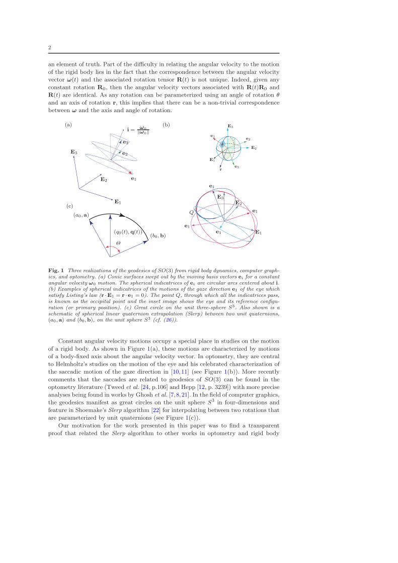
Fig. 1 Three realizations of the geodesics of SO(3) from rigid body dynamics, computer graph-ics, and optometry. (a) Conic surfaces swept out by the moving basis vectors ei for a constantangular velocity ω0 motion. The spherical indicatrices of ei are circular arcs centered about i.(b) Examples of spherical indicatrices of the motions of the gaze direction e1 of the eye whichsatisfy Listing’s law (r ·E1 = r ·e1 = 0). The point Q, through which all the indicatrices pass,is known as the occipital point and the inset image shows the eye and its reference configu-ration (or primary position). (c) Great circle on the unit three-sphere S3. Also shown is aschematic of spherical linear quaternion extrapolation (Slerp) between two unit quaternions,(a0,a) and (b0,b), on the unit sphere S3 (cf. (26)).

Constant angular velocity motions occupy a special place in studies on the motion

of a rigid body. As shown in Figure 1(a), these motions are characterized by motions

of a body-fixed axis about the angular velocity vector. In optometry, they are central

to Helmholtz’s studies on the motion of the eye and his celebrated characterization of

the saccadic motion of the gaze direction in [10,11] (see Figure 1(b)). More recently

comments that the saccades are related to geodesics of SO(3) can be found in the

optometry literature (Tweed et al. [24, p.106] and Hepp [12, p. 3239]) with more precise

analyses being found in works by Ghosh et al. [7,8,21]. In the field of computer graphics,

the geodesics manifest as great circles on the unit sphere S3 in four-dimensions and

feature in Shoemake’s Slerp algorithm [22] for interpolating between two rotations that

are parameterized by unit quaternions (see Figure 1(c)).

Our motivation for the work presented in this paper was to find a transparent

proof that related the Slerp algorithm to other works in optometry and rigid body

3

dynamics on the attitudes of constant angular velocity motions. We found that by

parameterizing the rotation using unit quaternions and then examining the necessary

conditions for geodesic motions of S3, an elegant and transparent set of differential

equations could be found. In contrast to other derivations of the differential equations,

such as Ghosh and Wijayasinghe [7, Eqn. (15)], O’Reilly and Payen [17, Eqn. (17)],

and Polpitiya et al. [21, Eqn (3)], the differential equations we find are linear, free from

singularities, and easily solved. In addition, the formulation of the equations using unit

quaternions readily leads to the Slerp algorithm, other characterizations of constant

angular velocity motions, and representations of the geodesics of SO(3) using Steiner’s

Roman surface.

We start the paper with a review of representations of a rotation and its associated

angular velocity vector using unit quaternions (also known as Euler parameters or

Euler-Rodrigues symmetric parameters [23]). The main novel results in the paper are

presented in Section 3 (in particular, equations (15) and (16)) and Section 5. The

remaining sections of the paper discuss the relationship between the geodesics found

in Section 3 to the Slerp algorithm in Section 4, and optometry in Section 7. Unit

quaternions form a two-to-one covering of the set of rotations SO(3). With the help

of Apery’s embedding of Steiner’s Roman surface, we show how the geodesics on S3

can be used to characterize the geodesics on SO(3) in Section 5 and, in the interest

of completeness, present representations of these geodesics as rigid body motions in

Section 6.

2 Background

An element of SO(3) can be uniquely identified with a proper-orthogonal matrix R.

After defining a fixed right-handed orthonormal basis {E1,E2,E3} for R3, we can use

this matrix to define a rotation tensor R:

R =

3∑

i=1

3∑

j=1

RijEi ⊗Ek. (1)

The tensor R is then used to define a corotational (also known as a body-fixed) basis

{e1, e2, e3}:

ek = REk =

3∑

i=1

RikEi, (k = 1, 2, 3) . (2)

Dating to Euler’s seminal work on rotations in the 18th century, it is known that a

rotation tensor is completely characterized by an axis of rotation r and an angle of

rotation θ. As a consequence of (2), the components of the unit vector r have the

unusual property that

rk = r ·Ek = r · ek, (k = 1, 2, 3) . (3)

Equivalently, the rotation can also be parameterized by a unit quaternion (q0,q) where

q0 = cos

(

θ

2

)

, q = sin

(

θ

2

)

r. (4)

4

The components Rik = ek · Ei of the tensor R have a particularly compact represen-

tation using unit quaternions:

R =

R11 R12 R13

R21 R22 R23

R31 R32 R33

=(

2q20 − 1)

1 0 0

0 1 0

0 0 1

+ 2

q21 q1q2 q1q3q1q2 q22 q2q3q1q3 q2q3 q23

+ 2q0

0 −q3 q2q3 0 −q1−q2 q1 0

. (5)

Here, qk = q · ek = q · Ek. Referring to (2), we note that the column vectors of the

matrix R define the components of the moving bases vectors relative to their fixed

counterparts and vice versa:

ek = R1kE1 +R2kE2 +R3kE3, Ek = Rk1e1 +Rk2e2 +Rk3e3. (6)

These identities will be used later to construct ei(t) given q0, q, and Ek.

The angular velocity vector ω is the axial vector of the skew-symmetric tensor

RR0 (RR0)T , where R0 is any constant tensor. This vector has the representations

ω = ω1e1 + ω2e2 + ω1e3

= 2q0q− 2q0q+ 2q× q. (7)

If ω is constant, then the components ωi are also necessarily constant. We also note that

ω determines ek, ek = ω × ek, and that the direction of ω defines the instantaneous

axis of rotation i:

i =ω

‖ω‖ . (8)

The axes r and i are parallel only in instances where r = 0.

3 Geodesics on S3: A dynamical systems approach

The geodesics of SO(3) can be motivated in a variety of manners. Here, we exploit a

classical construction and consider a spherically symmetric rigid body of mass m and

radius R =√

5

2. The rotational kinetic energy of the rigid body is simply T = m

2ω ·ω.

We use this energy to define the kinematical line-element ds for SO(3):

ds =

√

2T

mdt =

√ω · ωdt. (9)

Here,

ω · ω = 4q20 + 4q · q= 4q20 + 4q21 + 4q22 + 4q23 . (10)

The geodesics with respect to ds are extremizers of T and, appealing to Jacobi’s the-

orem, we note that T is conserved along the geodesics. Conservation of T also implies

that the angular speed√ω · ω is constant.

If we use unit quaternions or Euler parameters (also known as Euler-Rodrigues

symmetric parameters) to parameterize R, then a two-to-one covering of SO(3) is

5

obtained. That is, the pair of quaternions (q0,q) and (−q0,−q), correspond to the same

rotation. Thus, we first consider geodesics of S3 using the kinematical line-element ds.

The necessary conditions for (q0(t),q(t)) to correspond to a geodesic are

d

dt

(

∂T

∂qK

)

− ∂T

∂qK= λ1qK , (K = 0, 1, 2, 3) , (11)

where λ1 is a Lagrange multiplier associated with the Euler parameter constraint:

1 = q20 + q21 + q22 + q23 . (12)

Substituting for T , (11) reduce to

4mqK = λ1qK , (K = 0, 1, 2, 3) . (13)

These equations have the integral of motion T and we denote the value of this integral

of motion by T0.1

With the help of (12), we can solve for λ1:2

λ1 = −2T0. (14)

Hence, (11) reduce further to

qK +

(

T02m

)

qK = 0, (K = 0, 1, 2, 3) . (15)

These equations imply that the quaternion components associated with a geodesic

execute simple harmonic motions:

qK (t) = qK (0) cos (ν0t) +qK(0)

ν0sin (ν0t) , (16)

where the frequency ν0 is half the magnitude of ω:

ν20 =T02m

=ω · ω4

. (17)

The factor of one half in the angular speed of qK (t) compared to ei(t) can be attributed

to the fact that the unit quaternions provide a two-to-one cover for SO(3). The initial

conditions qK(0) and qK(0) must satisfy the Euler parameter constraint q0(0)q0(0) +

q(0) · q(0) = 1 and its differential counterpart q0(0)q0(0) + q(0) · q(0) = 0.

While the angular speed√ω · ω associated with the geodesic motions is constant,

this doesn’t guarantee that ω is a constant. However, as

ω = 2q0q− 2q0q+ 2q× q, (18)

and, from (13), mq0 = λ1

2q0 and mq = λ1

2q, we can conclude that ω is constant. Thus,

geodesics on S3 with respect to ds correspond to rotations with constant angular

velocity vectors.

1 While our construction of (13) follows from a variational principle for geodesics on aconfiguration manifold, the corresponding equations of motion also follow from those for therotational motion of a rigid body whose rotation is parameterized by Euler parameters. Theinterested reader is referred to [13,14,15,18] for a selection of derivations of the latter equations.

2 The curious fact that the Lagrange multiplier λ1 enforcing the Euler parameter constraintis proportional to T was first shown by Nikravesh et al. [15]. A continuum mechanics-basedinterpretation of λ1 can be found in [18].

6

The simplicity of the differential equations governing qK (t) enable us to quickly

conclude that q and q lie on a plane by noting the constancy of q× q:

d

dt(q× q) = q× q = 0. (19)

In the sequel, and without loss in generality, we often take advantage of this result by

choosing {E1,E2,E3} such that E1 is normal to the aforementioned plane: q1(0) =

q1(0) = 0. In this case, we can define the angle ψ such that (cf. (4))

q0 = cos

(

θ

2

)

, q2 = sin

(

θ

2

)

cos(ψ), q3 = sin

(

θ

2

)

sin(ψ), (20)

With the help of (16) it is straightforward to write down analytical expressions for θ(t)

and r(t):

θ(t) = 2 cos−1 (q0(t)) , ψ(t) = tan−1

(

q2(t)

q3(t)

)

, r(t) = cos(ψ(t))E1 + sin(ψ(t))E2.

(21)

While the closest related derivations known to us are Ghosh and Wijayasinghe [7],3

we believe the derivation of the representations (16) for the geodesics on S3 presented

here is simpler. In addition, the derivation of the representations (21) for r and θ(t)

are more transparent that those found in O’Reilly and Payen [17, Sect. 5]. We now

turn to showing how (16) are related to the quaternion interpolation formula featured

in computer graphics.

4 The Slerp algorithm for interpolating between a pair of rotations

An ingenious resolution to the problem of interpolating between two rotations in com-

puter graphics was proposed by Shoemake [22]. His solution was to parameterize both

rotations using unit quaternions and then interpolate between the pair of unit quater-

nions using a great circle on the unit sphere S3. The method is known as spherical

linear quaternion interpolation (Slerp).4

To see how Shoemake’s approach is consistent with (16) we return to (15) but

now consider the boundary-value problem of computing the geodesic that connects the

following pair of points on S3 (cf. Figure 1(c)):

(a0,a) = (a0, a1, a2, a3) , (b0,b) = (b0, b1, b2, b3) . (22)

We define Θ as the angle subtended by the vectors (a0, a) and (b0,b) in R4:

cos (Θ) = a0b0 + a1b1 + a2b2 + a3b3. (23)

As noted previously, the general solution to (15) is

qK (t) = AK cos (ν0t) +BK sin (ν0t) , (K = 0, 1, 2, 3) , (24)

3 See Theorem 2 and the nonlinear differential equations (15) in [7].4 Discussions of extensions to Shoemake’s work in the context of geodesics can be found in

Dam et al. [4], Park and Ravani [19] and Zefran and Kumar [25], among others.

7

where AK and BK are eight constants which we now determine. Choosing time t so that

(q0(0),q(0)) = (a0,a) and (q0 (t1) ,q (t1)) = (b0,b), we can solve for the 8 constants:

AK = aK , BK =1

sin (ν0t1)(bK − aK cos (ν0t1)) . (25)

Substituting into (24) and rearranging we find the final desired form:

qK(t) =1

sin (ν0t1){aK sin (ν0 (t1 − t)) + bK sin (ν0t)} . (26)

Identifying

Θ = ν0t1 = 0.5 ‖ω‖ t1, (27)

we conclude that the interpolation function (26) is none other that Shoemake’s Slerp

interpolation formula (cf. [4, Ch. 6, Sect. 1.5], [6, Eqn. (7)] and [22]). Typically, one

chooses t1 = 1 and hence the angular velocity of the interpolating motion is 2Θ and

the energy T0 of the motion is 2Θ2.

(a)

(b)

⋆

⋆⋆

⋆

⋆

⋆

⋆

⋆⋆

⋆

⋆

⋆

⋆

⋆

θ inc.

ψ inc.

R32

R32

R13

R13

R21

R21

q2

q2

q3

q3

q0

q0

1

1

1

1

1

1

1

1

1

1

1

1

−1

−1

−1

−1

−1

−1

−1

−1

−1

−1

−1

−1

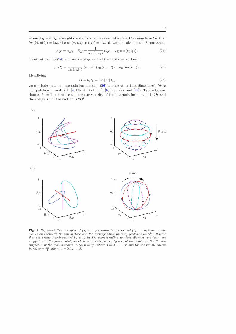
Fig. 2 Representative examples of (a) u = ψ coordinate curves and (b) v = θ/2 coordinatecurves on Steiner’s Roman surface and the corresponding pairs of geodesics on S2. Observethat six points (distinguished by a ⋆) in S2, corresponding to three distinct rotations, aremapped onto the pinch point, which is also distinguished by a ⋆, at the origin on the Romansurface. For the results shown in (a) θ = nπ

4where n = 0, 1, . . . , 8 and for the results shown

in (b) ψ = nπ

4where n = 0, 1, . . . , 8.

8

5 Geodesics of SO(3) and the immersion of the real projective plane RP2

Allowing for the fact that we can choose q1 = 0 without loss in generality, the remaining

coordinates to parameterize SO(3) are q2, q3 and q20 = 1 − q22 − q23 . Using the results

from Section 4, we know that the geodesics of SO(3) are circles on a two-sphere S2 in

R3. The sphere, however, still retains the two-to-one covering property between a pair

of antipodal points and a rotation R: (q0, q2, q3) and its antipodal point (−q0,−q2,−q3)describe the same rotation R. It is a well-known result in topology that the quotient

space of S2 obtained by identifying antipodal points is the real projective plane RP2.

Consequently, points in RP2 are isomorphic to SO(3) when q1 = 0 (cf. [1,5,21]).

Unfortunately, RP2 can be embedded in R4 but not R3. To proceed further, we immerse

RP2 into a non-orientable surface in R

3 which is known as Steiner’s Roman surface M[1,9].

The transformation required to perform the immersion is discussed in Apery’s

seminal work [1]:

F : (q0, q3, q2) 7→(

q2q3, q2q0, q3q0, q22 + q23 + q20

)

. (28)

However, from (5) and (6), we find that

2q2q3 = R32 = e2 ·E3,

2q2q0 = R13 = e3 ·E1,

2q3q0 = R21 = e1 ·E2. (29)

Thus by projecting into R3, we arrive at the desired mapping

G : (q0, q3, q2) 7→ (R32, R13, R21) . (30)

We next recast the parametric equations for the two-dimensional manifold M, known

as Steiner’s Roman surface, in R3 by representing the quaternion components as a

function of azimuthal and zenith angles on S2: {u, v} ={

ψ, θ2

}

(cf. (20)). The resulting

expressions for the Cartesian coordinates of a point on M are

x1(u, v) = R32 = 2q2q3 = sin(2u) sin2(v) = sin(2ψ) sin2(

θ

2

)

, (31)

x2(u, v) = R13 = 2q2q0 = cos(u) sin(2v) = cos(ψ) sin (θ) , (32)

x3(u, v) = R21 = 2q0q3 = sin(u) sin(2v) = sin(ψ) sin (θ) . (33)

Although M is a non-orientable surface in R3, all but three rotations can be identified

with a single point on M (see Figure 2).5 The exceptions are the three rotations

(r = E2, θ = π), (r = E3, θ = π), and the identity R = I. Each of these three rotations

are mapped to the origin (also known as the triple point or pinch point of M). Because

the rotations associated with the triple point are not unique, it is possible to have a

closed trajectory starting from and ending at the triple point where the body does not

return to its starting orientation. We also observe from the u- and v-coordinate curves

and the corresponding geodesics on S2 displayed in Figure 2, that generically pairs of

curves on S3 map to a single line or curve on M.

5 The space {x1, x2, x3} which contains M, can also be considered as a projection of the nine-dimensional Euclidean configuration space R

9, whose Cartesian coordinates are componentsof the rotation tensor R (cf. Casey [3]).

9

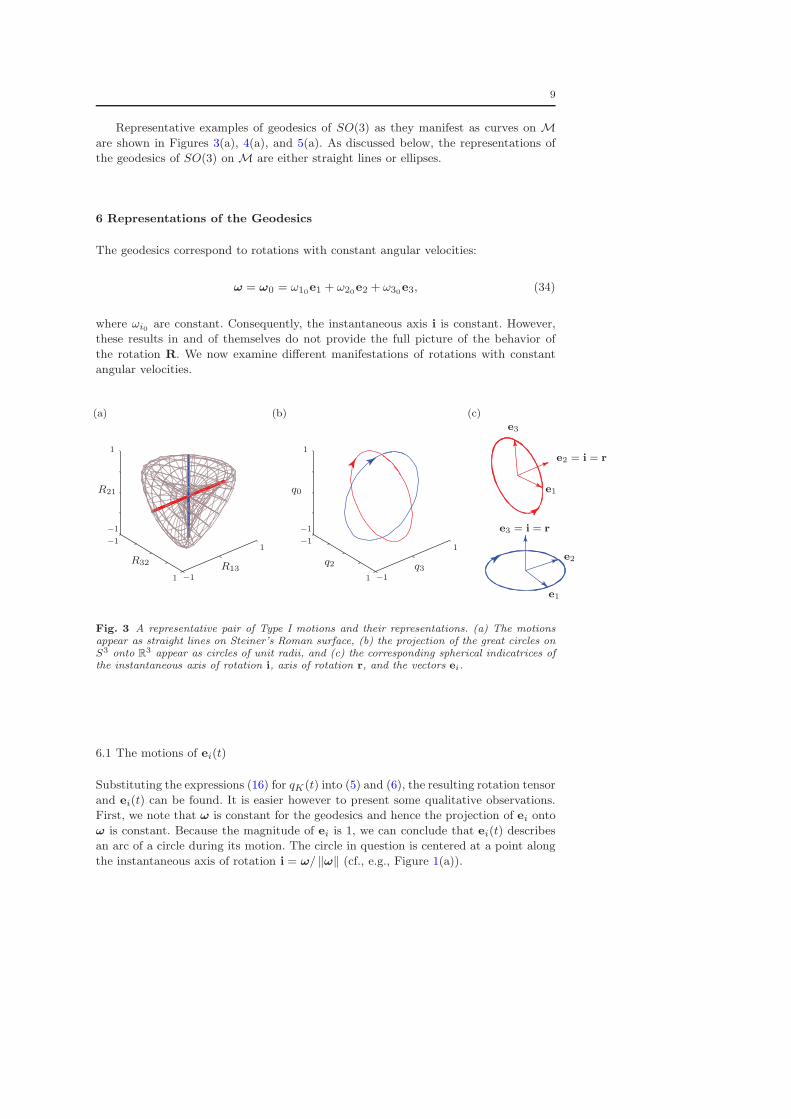
Representative examples of geodesics of SO(3) as they manifest as curves on Mare shown in Figures 3(a), 4(a), and 5(a). As discussed below, the representations of

the geodesics of SO(3) on M are either straight lines or ellipses.

6 Representations of the Geodesics

The geodesics correspond to rotations with constant angular velocities:

ω = ω0 = ω10e1 + ω20e2 + ω30e3, (34)

where ωi0 are constant. Consequently, the instantaneous axis i is constant. However,

these results in and of themselves do not provide the full picture of the behavior of

the rotation R. We now examine different manifestations of rotations with constant

angular velocities.

(a) (b) (c)

e1

e1

e2

e3

e2 = i = r

e3 = i = r

R13

R32

R21 q0

q2 q31

1

1

1

1

1

−1

−1

−1

−1

−1

−1

Fig. 3 A representative pair of Type I motions and their representations. (a) The motionsappear as straight lines on Steiner’s Roman surface, (b) the projection of the great circles onS3 onto R

3 appear as circles of unit radii, and (c) the corresponding spherical indicatrices ofthe instantaneous axis of rotation i, axis of rotation r, and the vectors ei.

6.1 The motions of ei(t)

Substituting the expressions (16) for qK(t) into (5) and (6), the resulting rotation tensor

and ei(t) can be found. It is easier however to present some qualitative observations.

First, we note that ω is constant for the geodesics and hence the projection of ei onto

ω is constant. Because the magnitude of ei is 1, we can conclude that ei(t) describes

an arc of a circle during its motion. The circle in question is centered at a point along

the instantaneous axis of rotation i = ω/ ‖ω‖ (cf., e.g., Figure 1(a)).

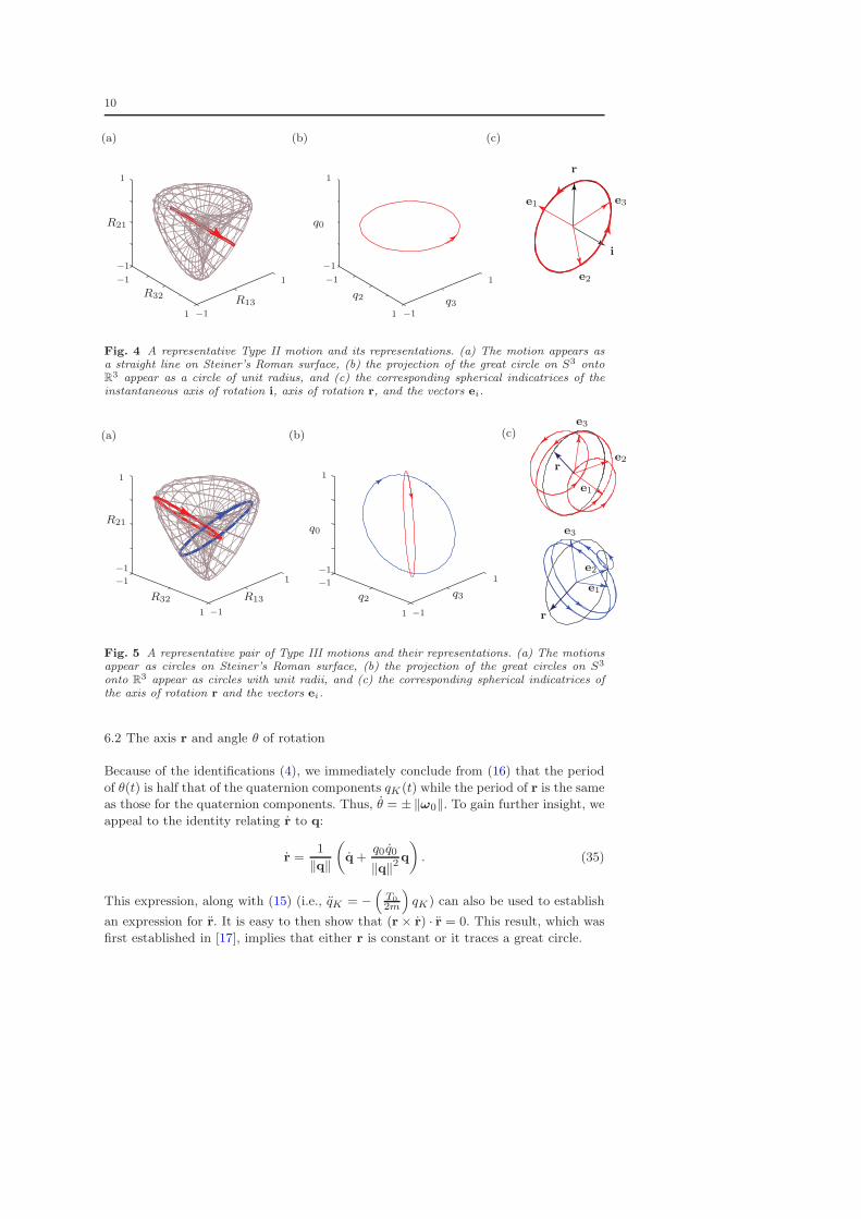
10

(a) (b) (c)

e1

e2

e3

R13

R32

R21 q0

q2 q31

1

1

1

1

1

−1

−1

−1

−1

−1

−1

r

i

Fig. 4 A representative Type II motion and its representations. (a) The motion appears asa straight line on Steiner’s Roman surface, (b) the projection of the great circle on S3 ontoR3 appear as a circle of unit radius, and (c) the corresponding spherical indicatrices of the

instantaneous axis of rotation i, axis of rotation r, and the vectors ei.

(a) (b) (c)

e1

e1

e2

e2

e3

e3

r

r

R13R32

R21q0

q2 q3

1

1

1

1

1

1

−1

−1

−1

−1

−1

−1

Fig. 5 A representative pair of Type III motions and their representations. (a) The motionsappear as circles on Steiner’s Roman surface, (b) the projection of the great circles on S3

onto R3 appear as circles with unit radii, and (c) the corresponding spherical indicatrices of

the axis of rotation r and the vectors ei.

6.2 The axis r and angle θ of rotation

Because of the identifications (4), we immediately conclude from (16) that the period

of θ(t) is half that of the quaternion components qK (t) while the period of r is the same

as those for the quaternion components. Thus, θ = ±‖ω0‖. To gain further insight, we

appeal to the identity relating r to q:

r =1

‖q‖

(

q+q0q0

‖q‖2q

)

. (35)

This expression, along with (15) (i.e., qK = −(

T0

2m

)

qK) can also be used to establish

an expression for r. It is easy to then show that (r× r) · r = 0. This result, which was

first established in [17], implies that either r is constant or it traces a great circle.

11

Choosing E1 to be normal to r (without loss of generality), we previously arrived

at the analytical expressions (21) for r(t) and θ(t). These expressions are consistent

with the results of [17]. Consequently, we appeal to [17] who found that rotations with

constant angular velocity motions can be classified into three types:

Type I. Motions where the axis of rotation is parallel to ω and θ is a non-zero constant:

q ‖ i and q× q = 0 (cf. Figure 3).

Type II. Motions where θ = π and the axis of rotation is perpendicular to ω. That is, q0 = 0

and q · ω = 0 (cf. Figure 4).

Type III. Motions where θ = θ(t) but r is neither normal to nor parallel to ω. That is, q0 6= 0

and q · ω 6= 0 (cf. Figure 5).

Type I motions are prototypical constant angular velocity motions and, given the free-

dom to choose the reference basis {E1,E2,E3} or, equivalently, R0, constant angular

velocity motions can always be restricted to this type. Unfortunately, in many appli-

cation areas, such as opthomology, the reference basis for R is prescribed and Type II

and Type III motions must be considered.

7 Saccadic Motions of the Eye

Dating to Helmholtz’s works on the eye [10,11], constant angular velocity motions have

played a central role in understanding saccadic motions of the eye. When modeled

as a rotating rigid body, the motion of the eye is subject to a constraint known as

Listing’s constraint. While Listing’s law dates to the mid 1800s, formulating the law

using quaternions was championed by Westheimer [26] a century later. If the gaze

direction of the eye is modeled as e1, then Listing’s constraint can be expressed in the

equivalent forms

q · E1 = 0, q · e1 = 0. (36)

That is the axis of rotation of the eye lies at the intersection of a plane fixed in the eye

(the focal plane) and a plane fixed in the head (cf. Figure 1(b)). Of particular interest

in optometry are the possible motions of the gaze direction e1.

If one models the eye as a spherically symmetric rigid body, then the geodesics of

interest are those of SO(3) which satisfy Listing’s law. With little extra work, we arrive

at the following set of differential equations in place of (15):

4q0 + 2λ1q0 = 0, λ2 = 0, 4q2 + 2λ1q2 = 0, 4q3 + 2λ1q3 = 0, (37)

where λ2 is the Lagrange multiplier that ensures that Listing’s constraint holds. We

again find that λ1 = −T0 (albeit with q1 = 0) and also that λ2 = 0.6 Consequently, the

geodesics on the subspace of SO(3) that satisfy Listing’s law are given by (16)K=0,2,3

and the earlier characterizations and representations apply. Conversely, many supple-

mental results, such as Listing’s half-angle rule and Helmholtz’s theorem [11,24] can

be imported from optometry and use to provide additional insight into the geodesics

(see [16] for additional references and discussion).

6 The result that λ2 = 0 was first shown, using a different formulation, by Cannata andMaggiali [2].

12

8 Closing Remarks

The characterizations of the geodesics we have provided assume that the metric is

given by the line-element ds (9). If we change this element, for instance we could use

the kinetic energy expression for an axisymmetric or asymmetric rigid body, then the

geodesics will change. In particular, some of the geodesics will feature non-constant

angular velocity vectors. Further, while closed-form analytical solutions for the an-

gular velocity components ωi(t) of the moment-free motion of an axisymmetric and

asymmetric rigid bodies, computing the corresponding rotations is non-trivial and the

geodesics may manifest as quasiperiodic motions of ei(t).

Acknowledgements

We take this opportunity to thank Prof. Kenneth A. Ribet (U. C. Berkeley) for several

helpful comments on the connections between SO(3) and RP2.

References

1. Apery, F.: Models of the Real Projective Plane: Computer Graphics of Steiner and BoySurfaces. Computer graphics and mathematical models. Vieweg+Teubner Verlag (1987)

2. Cannata, G., Maggiali, M.: Models for the design of bioinspired roboteyes. IEEE Transactions on Robotics 24(1), 27–44 (2008). URLhttp://dx.doi.org/10.1109/TRO.2007.906270

3. Casey, J.: On the representation of rigid body rotational dynamics in Hertzian configura-tion space. International Journal of Engineering Science 49(12), 1388–1396 (2011). URLhttp://dx.doi.org/10.1016/j.ijengsci.2011.03.012

4. Dam, E.B., Koch, M., Lillholm, M.: Quaternions, interpolation and an-imation. Datalogisk Institut, Københavns Universitet (1998). URLhttp://web.mit.edu/2.998/www/QuaternionReport1.pdf

5. Demiralp, C., Hughes, J.F., Laidlaw, D.H.: Coloring 3D line fields using Boy’s real projec-tive plane immersion. IEEE Transactions on Visualization and Computer Graphics 15(6),1457–1464 (2009). URL http://dx.doi.org/10.1109/TVCG.2009.125

6. Ge, Q.J., Ravani, B.: Geometric construction of Bezier motions. ASME Journal of Me-chanical Design 116(3), 749–755 (1995). URL http://dx.doi.org/10.1115/1.2919446

7. Ghosh, B., Wijayasinghe, I.: Dynamics of human head and eye rotations under Donders’constraint. Automatic Control, IEEE Transactions on 57(10), 2478–2489 (2012). URLhttp://dx.doi.org/10.1109/TAC.2012.2186183

8. Ghosh, B., Wijayasinghe, I., Kahagalage, S.: A geometric approach to head/eye control.Access, IEEE 2, 316–322 (2014). URL http://dx.doi.org/10.1109/ACCESS.2014.2315523

9. Gray, A.: Modern Differential Geometry of Curves and Surfaces with Mathematica. CRCPress, Inc., Boca Raton, FL, USA (1996)

10. Helmholtz, H.: Ueber die normalen Bewegungen des menschlichen Auges. Archiv furOphthalmologie 9(2), 153–214 (1863). URL http://dx.doi.org/10.1007/BF02720895

11. von Helmholtz, H.: A Treatise on Physiological Optics, vol. III. Dover Publications, NewYork (1962). Translated from the (1910) third German edition and edited by J.P.C.Southall

12. Hepp, K.: Theoretical explanations of Listing’s law and their implicationfor binocular vision. Vision Research 35(23–24), 3237–3241 (1995). URLhttp://dx.doi.org/10.1016/0042-6989(95)00104-M

13. Moller, M., Glocker, C.: Rigid body dynamics with a scalable body, quaternionsand perfect constraints. Multibody System Dynamics 27(4), 437–454 (2012). URLhttp://dx.doi.org/10.1007/s11044-011-9276-5

14. Morton, H.S.J.: Hamiltonian and Lagrangian formulations of rigid body rotational dy-namics based on Euler parameters. Journal of the Astronautical Sciences 41(4), 569–591(1993)

13

15. Nikravesh, P.E., Wehage, R.A., Kwon, O.K.: Euler parameters in computational kinemat-ics and dynamics. Part 1. ASME Journal of Mechanisms, Transmissions, and Automationin Design 107(3), 358–365 (1985). URL http://dx.doi.org/10.1115/1.3260722

16. Novelia, A., O’Reilly, O.M.: On the dynamics of the eye: Geodesics on a configurationmanifold, motions of the gaze direction and Helmholtz’s theorem. Nonlinear Dynamics80(3), 1303–1327 (2015). URL http://dx.doi.org/10.1007/s11071-015-1945-0

17. O’Reilly, O.M., Payen, S.: The attitudes of constant angular velocitymotions. Internat. J. Non-Linear Mech. 41(6–7), 1–10 (2006). URLhttp://dx.doi.org/10.1016/j.ijnonlinmec.2006.05.001

18. O’Reilly, O.M., Varadi, P.C.: Hoberman’s sphere, Euler parameters andLagrange’s equations. J. Elasticity 56(2), 171–180 (1999). URLhttp://dx.doi.org/10.1023/A:1007624027030

19. Park, F.C., Ravani, B.: Bezier curves on Riemannian manifolds and Lie groups with kine-matics applications. ASME Journal of Mechanical Design 117(1), 36–40 (1995). URLhttp://dx.doi.org/10.1115/1.2826114

20. Poinsot, L.: Outlines of a New Theory of Rotatory Motion, Translated from the French ofPoinsot with Explanatory Notes. Cambridge University Press, London (1834). Translatedfrom the French article “Theorie nouvelle de la rotation des corps presentee a l’Institut le19 Mai 1834” by C. Whitley

21. Polpitiya, A., Dayawansa, W., Martin, C., Ghosh, B.: Geometry and control of humaneye movements. IEEE Transactions on Automatic Control 52(2), 170–180 (2007). URLhttp://dx.doi.org/10.1109/TAC.2006.887902

22. Shoemake, K.: Animating rotation with quaternion curves. In: Proceedings ofthe 12th Annual Conference on Computer Graphics and Interactive Techniques,SIGGRAPH ’85, pp. 245–254. ACM, New York, NY, USA (1985). URLhttp://doi.acm.org/10.1145/325334.325242

23. Shuster, M.D.: A survey of attitude representations. The Journal of the AstronauticalSciences 41(4), 439–517 (1993)

24. Tweed, D., Cadera, W., Vilis, T.: Computing three-dimensional eye position quaternionsand eye velocity from search coil signals. Vision Research 30(1), 97–110 (1990). URLhttp://dx.doi.org/10.1016/0042-6989(90)90130-D

25. Zefran, M., Kumar, V.: Interpolation schemes for rigid body motions. Computer-Aided De-sign 30(3), 179–189 (1998). URL http://dx.doi.org/10.1016/S0010-4485(97)00060-2

26. Westheimer, G.: Kinematics of the eye. Journal of the Optical Society of America 47(10),967–974 (1957). URL http://dx.doi.org/10.1364/JOSA.47.000967