On generating tight Gabor frames at critical

density

A.J.E.M. Janssen

Philips Research Laboratories WY-81,

5656 AA Eindhoven, The Netherlands

e-mail: A.J.E.M.Janssen@philips.com

Abstract.

We consider the construction of tight Gabor frames (h, a = 1, b = 1) from

Gabor systems (g, a = 1, b = 1) with g a window having few zeros in theZak transform domain via the operation h = Z�1(Zg=jZgj), where Z is thestandard Zak transform. We consider this operation with g the Gaussian, the

hyperbolic secant, and for g belonging to a class of positive, even, unimodal,rapidly decaying windows of which the two-sided exponential is a typical ex-

ample. All these windows g have the property that Zg has a single zero, viz.at (1

2; 12), in the unit square [0; 1)2. The Gaussian and hyperbolic secant yield

a frame for any a; b > 0 with ab < 1, and we show that so does the two-sided

exponential. For these three windows it holds that S�1=2a g ! h as a " 1,where Sa is the frame operator corresponding to the Gabor frame (g; a; a).It turns out that the h's corresponding to g's of the above type look and

behave quite similarly when scaling parameters are set appropriately. We

give a particular detailed analysis of the h corresponding to the two-sided

exponential. We give several representations of this h, and we show thath 2 L1(R) \ L1(R), and is continuous and di�erentiable everywhere exceptat the half-integers, etc., and we pay particular attention to the cases that

the time constant of the two-sided exponential g tends to 1. We also con-

sider the cases that the time constants of the Gaussian and of the hyperbolicsecant tend to 0 or to 1. It so turns out that h thus obtained changes from

the box function �(�1=2;1=2) into its Fourier transform sinc �� when the timeconstant changes from 0 to 1.

AMS Subject Classi�cation: 42C15, 94A12, 33E05.

Keywords: Gabor frame, tight frame, Zak transform, critical density.

1

1 Introduction

We consider in this paper Gabor systems and frames, in particular tight

Gabor frames, at critical density. We assume the reader to be somewhat

familiar with Gabor theory and the basic notions in this theory, such as frame,

frame operator, frame bounds, tight frame, dual frame, Zak transform, etc.

To �x notations, we denote for x; y 2 R and g 2 L2(R)

g(x; y)(t) = e2�iyt g(t� x) ; a:e: t 2 R : (1)

When a > 0, b > 0 and g 2 L2(R), we call the collection of functions

fg(na;mb) jn;m 2 Zg a Gabor system which we denote by (g; a; b). Such a

system is called a Gabor frame when there are A > 0, B <1 such that for

all f 2 L2(R)

A kfk2 �Xn;m

j(f; g(na;mb))j2 � B kfk2 : (2)

Here k k and ( ; ) are the standard norm and inner product of L2(R). Wecall A a lower frame bound and B an upper frame bound of the Gaborsystem (g; a; b). We refer to [1]{[3] for generalities about frames for a Hilbert

space and for both basic and in- depth information about Gabor framesand related matters. A very recent and comprehensive treatment of modernGabor theory can be found in [4], in particular Chs. 5{9, 11{13.

In this paper we are interested in the tight frames at critical densitya = b = 1, where tightness means that A = B = 1 in (2). It is well known,

see for instance [4], Corollary 7.5.2, that (h, a = 1, b = 1) is a tight Gaborframe if and only if (h(n;m))n;m2Z is an orthonormal base for L2(R). Anothercharacterization of tightness is obtained in terms of the Zak transform. When

f 2 L2(R) we let

(Zf)(t; �) =1X

k=�1

f(t� k) e2�ik� ; a:e: t; � 2 R ; (3)

and we call Zf the Zak transform of f , see [4], Ch. 8. Then we have that (h,

a = 1, b = 1) is a tight Gabor frame if and only if

j(Zh)(t; �)j = 1 ; a:e: t; � 2 R : (4)

It is well known that a window h such that (h, a = 1, b = 1) is a tightframe, cannot be too well-behaved in terms of smoothness and decay, see for

instance [4], Theorem 8.4.5 (Balian-Low theorem). Two examples of an h for

which (h, a = 1, b = 1) is a tight frame are

h = �(�1=2;1=2) ; h = F �(�1=2;1=2) = sinc� � ; (5)

2

where F denotes the Fourier transform, (Ff)(�) = Rexp(�2�i�t) f(t) dt for

f 2 L2(R). The Zak transform of the two windows in (5) are given by

(Z �(�1=2;1=2))(t; �) = 1 ; (Z F �(�1=2;1=2))(t; �) = e2�it� ; a:e: (t; �) 2 [0; 1)2 ;

(6)

respectively.

One can generate tight frames (h, a = 1, b = 1) as follows. Given a

well-behaved window g 2 L2(R) such that Zg is a continuous function with

few zeros per unit square, set

h = Z�1(Zg=jZgj) ; (7)

with Z�1 the inverse Zak transform. That is

h(t) =

1Z0

(Zg)(t; �)

j(Zg)(t; �)j d� ; a:e: t 2 R : (8)

Obviously this h satis�es (4). In this paper we consider in particular thechoices

g1; (t) = (2 )1=4 e�� t2

; g2; (t) =�� 2

�1=2 1

cosh � t; t 2 R ; (9)

(Gaussian and hyperbolic secant) with > 0, and

g3;�(t) = �1=2 e��jtj ; t 2 R ; (10)

(two-sided exponential) with � > 0. The normalizations in (9) and (10) aresuch that the g's have unit L2-norm. Note that the two windows in (9) are

smooth and rapidly decaying; they even have a Fourier invariance property

in the sense that F g1; = g1;1= , F g2; = g2;1= . The two-sided exponential in(10) is an example of a window of, what we call, type II, see [5], Subsec. 2.2.

The latter windows are even, positive and integrable on R, and satisfy a

convexity condition on [0;1); in particular, g0 has a jump at t = 0 for such

a window g. The Zak transforms of the windows in (9) and those of windows

of type II all have exactly one zero, viz. at (12; 12), in the unit square [0; 1)2,

whence the de�nition of h according to (7) makes sense. In this paper we

shall investigate the windows h produced by the operation (7), where we payparticular attention to the cases that g is one of the windows in (9) and (10).

Although we present all our results directly in terms of h(t) itself, it is

well worth noting that a number of these results hold when h is replaced byits Fourier transform F h. Indeed, it follows from the relation

(Z F f)(t; �) = e2�i�t(Zf)(��; t) ; a:e: t; � 2 R ; (11)

3

holding for f 2 L2(R), that the operation g ! h = Z�1(Zg=jZgj) commutes

with the Fourier transform. Moreover, g is even and real if and only if Fgis. Finally, by the quasi-periodicity relations of the Zak transform and (11),

we have that Zg has a single zero at (12; 12) in the unit square [0; 1)2 if and

only if Z F g has, and the nature of these zeros is the same.

2 Overview of results

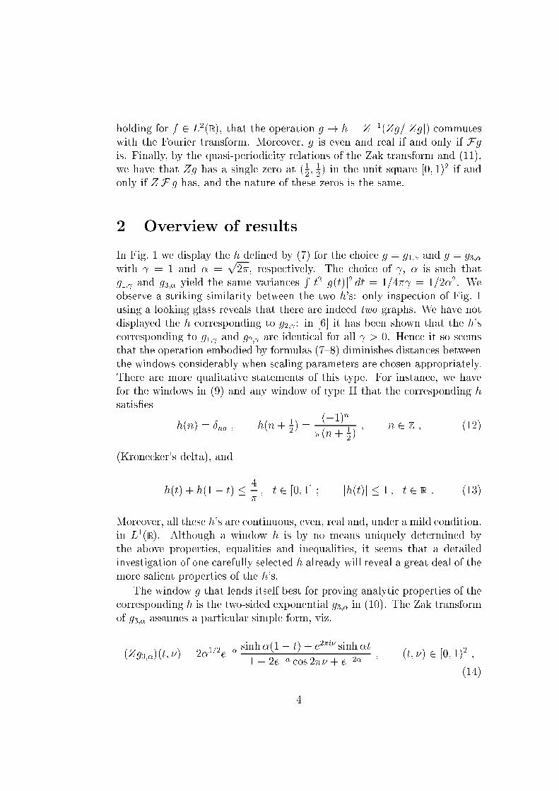
In Fig. 1 we display the h de�ned by (7) for the choice g = g1; and g = g3;�with = 1 and � =

p2�, respectively. The choice of , � is such that

g1; and g3;� yield the same variancesRt2 jg(t)j2 dt = 1=4� = 1=2�2. We

observe a striking similarity between the two h's: only inspection of Fig. 1using a looking glass reveals that there are indeed two graphs. We have notdisplayed the h corresponding to g2; : in [6] it has been shown that the h's

corresponding to g1; and g2; are identical for all > 0. Hence it so seemsthat the operation embodied by formulas (7{8) diminishes distances betweenthe windows considerably when scaling parameters are chosen appropriately.

There are more qualitative statements of this type. For instance, we havefor the windows in (9) and any window of type II that the corresponding h

satis�es

h(n) = Æno ; h(n + 12) =

(�1)n�(n+ 1

2); n 2 Z ; (12)

(Kronecker's delta), and

h(t) + h(1� t) � 4

�; t 2 [0; 1] ; jh(t)j � 1 ; t 2 R : (13)

Moreover, all these h's are continuous, even, real and, under a mild condition,in L1(R). Although a window h is by no means uniquely determined bythe above properties, equalities and inequalities, it seems that a detailed

investigation of one carefully selected h already will reveal a great deal of the

more salient properties of the h's.

The window g that lends itself best for proving analytic properties of the

corresponding h is the two-sided exponential g3;� in (10). The Zak transform

of g3;� assumes a particular simple form, viz.

(Zg3;�)(t; �) = 2�1=2e��sinh�(1� t) + e2�i� sinh�t

1� 2e�� cos 2�� + e�2�; (t; �) 2 [0; 1)2 ;

(14)

4

see [7] and Prop. 5.1. Accordingly, h3;� (the h corresponding to g = g3;�under the mapping (7{8)) is given by

h3;�(t + n) =

1Z0

1 + r(t) e2�i�

j1 + r(t) e2�i�j e2�in� d� ; t 2 [0; 1) ; n 2 Z ; (15)

where

r(t) = sinh�t=sinh�(1� t) ; 0 � t < 1 : (16)

The forms (15{16) for h3;� give rise to a number of representations of h3;�that are useful for showing analytic results.

Let us now describe the further contents of this paper. In Sec. 3 we

show the following. Assume that g is a smooth and rapidly decaying window

such that Zg has a �nite number of zeros in the unit square [0; 1)2. Alsoassume that (g; a; a) is a Gabor frame for all a 2 (0; 1), and denote by Sa thecorresponding frame operator, i.e.

Sa f =Xn;m

(f; g(na;ma)) g(na;ma) ; f 2 L2(R) : (17)

Then

lima"1

S�1=2a g = h = Z�1(Zg=jZgj) ; (18)

where the limit is in L2(R)-sense. We observe that S�1=2a g is the tight framegenerating window canonically associated with the Gabor frame (g; a; a), see[8] for characterization and computation of these windows S�1=2a g.

In Sec. 4 we consider even, positive, continuous, rapidly decaying windowsg, and we list how symmetry properties of g are re ected by corresponding

properties of the Zak transforms Zg. These symmetry properties are then

also shown to hold for h = Z�1(Zg=jZgj). We furthermore show in Sec. 4

that h 2 L1(R) when Zg has a single zero, at (12; 12), in the unit square [0; 1)2

and@ Zg

@t(12; 12) 6= 0 6= @ Zg

@�(12; 12) : (19)

We also show the properties, equalities and inequalities mentioned in con-

nection with (12) and (13).

It is well known that (g1; ; a; b) is a frame when a; b > 0 and ab <

1; recently a corresponding result has been shown for the Gabor systems(g2; ; a; b), see [6]. In Sec. 5 we shall show that (g3;�; a; b) is a frame whena; b > 0 and ab < 1. The approach to the proof of the latter result is basi-

cally the same as the one to the main result in [6], but the details are quite

di�erent.

5

In Sec. 6 we shall present a detailed analysis of h3;� = Z�1(Zg3;�=jZg3;�j).This analysis is based on integral representations of h3;�, like the direct one

in (15) or the representation (we set r = r(t) for convenience)

h3;�(t+n) =(�1)n�

min(r;1=r)Z0

vn�1=2s1� rv

r � vdv ; t 2 [0; 1) ; n = 0; 1; ::: ;

(20)

that follows from the direct one, as well as on certain series representations

of h3;�(t + n). These representations are used to show that

(a) h3;� is positive and decreasing on [0; 1),

(b) (�1)n h3;�(t+ n) > 0, t 2 [0; 1), n = 0; 1; ::: ,

(c) (�1)n h03;�(t+ n) < 0, t 2 [12; 1), n = 0; 1; ::: ,

(d) (�1)n h03;�(n+ 12) = �1, n = 0; 1; ::: .

Furthermore, bounds on h3;� and asymptotics of h3;�(t + n) as n ! 1 andt 2 [0; 1) is �xed can be derived. As a consequence we can get a more

precise version of the statement shown in Sec. 4 that h 2 L1(R). We also payattention in Sec. 6 to the way the misbehaviour of g3;� at t = 0 is re ected

by corresponding misbehaviour or h3;� at t = n, n integer.

In Sec. 7 we consider the case that � # 0 in more detail. Then we getr(t) = t=(1� t) in (16). Note that h3;� can be expressed in terms of h3;0 by

the warping operation

h3;�(t+n) = h3;0( �(t)+n) ; �(t) =r(t)

1 + r(t); 0 � t < 1 ; n = 0; 1; ::: :

(21)

We shall compute explicitly in Sec. 7 that for n = 0; 1; :::

1=2Z0

jh3;0(t+n)j dt =�12+1

�

�Hn ;

1Z1=2

jh3;0(t+n)j dt =�12� 1

�

�Hn ; (22)

where

Hn =

1Z0

jh3;0(t + n)j dt = 2(�1)n��4�

n�1Xk=0

(�1)k2k + 1

� (�1)n2(2n+ 1)

�: (23)

From this it follows that kh3;0k1 = 12�.

6

In Sec. 8 we consider the case that g = g1; or g2; and !1 or # 0;recall that in [6] it has been shown that h := h1; = h2; for all > 0. We

show that

lim !1

h = �(�1=2;1=2) ; lim #0

h = sinc � � ; (24)

where the limits are in L2(R)-sense. We shall furthermore present a simple

condition on a window g such that the limit formulas (24) hold, more gener-

ally, for the tight frame generating window h corresponding to the window

1=2 g( �). Thus one obtains a whole class of families ((h )n;m)n;m2Z of rea-

sonably behaved orthonormal Gabor bases (tight Gabor frames at critical

density a = b = 1) that interpolate smoothly between the Gabor bases gen-

erated by the box function at = 1 and its Fourier transform sinc�� at = 0, compare (5).

3 Zak tight windows as limits of frame tight

windows

In this section we prove the following result.

Theorem 3.1. Assume that we have a g 2 L2(R) such that (g; g(x; y))is rapidly decaying in x; y 2 R, see (1), and that Zg has a �nite number ofzeros in the unit square [0; 1)2. Also assume that (g; a; a) is a frame for all

a 2 (0; 1), with frame operator Sa. Then there holds

lima"1

S�1=2a g = h = Z�1(Zg=jZgj) (25)

in L2(R)-sense.

Proof. Denote ah = S�1=2a g for a 2 (0; 1). The proof uses the followingsteps.

(a) kahk = a, khk = 1,

(b) Sa ! S1 strongly as a " 1 (S1 is the operator in (17) with a = 1),

(c) S1=2a ! S

1=21 strongly as a " 1,

(d) (ah; k)! (h; k) as a " 1 for all k of the form k = S1=21 f with f 2 L2(R),

(e) ah! h weakly as a " 1,

(f) kah� hk ! 0 as a " 1.

7

Ad (a). This follows from the well-known Wexler-Raz duality condition and

the de�nition of h, ah.

Ad (b). In Janssen's representation, see [4], Subsec. 7.2,

Sa f =1

a2

Xk;l

(g; g(k=a; l=a)) f(k=a; l=a) ; f 2 L2(R) ; (26)

there is absolute convergence of the right-hand side series. By continuity and

rapid decay of (g; g(x; y)) (also see Note 3 below and (33){(35)) we have that

Sa f ! S1 f as a " 1 and f 2 L2(R).

Ad (c). Approximate x1=2 uniformly on [0; B] by polynomials, where B

is an upper frame bound for all systems (g; a; a) with 12� a � 1. Use the

spectral mapping theorem for the positive semi-de�nite operators Sa, S1 to

get polynomial approximations to S1=2a , S

1=21 in the strong operator topology,

and �nally we use that Sa ! S1 strongly implies that Sna ! Sn

1 strongly for

all n = 0; 1; ::: .

Ad (d)). Let k = S1=21 f with f 2 L2(R). Below we show that for 0 < a < 1

g = S1=21 h = S1=2

aah : (27)

From this it follows that

(ah� h; k) = (ah� h; S1=21 f) = (ah; S

1=21 f)� (g; f) : (28)

We also have

(ah; S1=21 f) = (ah; S1=2

a f) + (ah; (S1=21 � S1=2

a )f) =

= (g; f) + o(1) ; a " 1 ; (29)

by (27) and (a), (c). Hence (ah� h; k)! 0 as a " 1.We now show (27). Clearly we have g = S

1=21

ah since ah = S�1=2a g. To

show that g = S1=21 h we let " > 0. By functional calculus in the Zak trans-

form domain for S1, see for instance [8], Subsec. 1.1 (in particular formulas

(37) or (38)), we have

Z [(S1 + "I)1=2 f ] = (jZgj2 + ")1=2 Zf ; f 2 L2(R) : (30)

Letting " # 0 and using strong convergence of (S1 + "I)1=2 to S1=21 , we see

that

Z [S1=21 f ] = jZgjZf ; f 2 L2(R) : (31)

8

Now taking f = h in (31) and using the de�nition of h we easily obtain

Zg = Z(S1=21 h), i.e. g = S

1=21 h.

Ad (e). We shall show that the set of all k = S1=21 f with f 2 L2(R) is

dense in L2(R). From (a) and (d) it then follows that ah ! h weakly as

a " 1.By assumption Zg is continuous and has �nitely many zeros in [0; 1)2.

Hence the set jZgj � F with F 2 L2([0; 1)2) is dense in L2([0; 1)2). The

mapping Z is a unitary operator from L2(R) onto L2([0; 1)2), whence the set

jZgj �Zf with f 2 L2(R) is dense in L2([0; 1)2). Then from (31) and unitarity

of Z it follows that the set S1=21 f with f 2 L2(R) is dense in L2(R).

(f). This follows easily from (a) and (e).

Notes.

1. We could have considered equally well Gabor frames (g; a; b) or (g; a; 1)or (g; 1; b) as a " 1 and/or b " 1 with corresponding frame operators.

2. Assume that (g; 1; 1) has a �nite upper frame bound while Zg is contin-

uous and has �nitely many zeros in the unit square. Then

lim"#0

(S1 + "I)�1=2 g = h (32)

in L2(R)-sense. This follows on inspecting the arguments used to prove(d) and (e).

3. The author was kindly informed by H.G. Feichtinger that he and G. Zim-mermann have shown that (b) in the proof holds on the assumption that

g 2 S0(R), see [3], ch. 3 for information on S0(R) (private communication).

We check the condition of continuity and rapid decay of (g; g(x; y)) as a

function of x; y 2 R for the cases that g = g1; ; g2; ; g3;�, see (9), (10). There

holds, explicitly,

(g1; ; g1; (x; y)) = e��ixy e�12� x2�

12�y2= ; (33)

(g2; ; g2; (x; y)) =� e��ixy sin�xy

sinh � x sinh�y= ; (34)

(g3;�; g3;�(x; y)) = � e��ixy e��jxjn� cos � jxj y�2 + �2y2

+�2 sin� jxj yy(�2 + �2y2)

o(35)

9

for x; y 2 R. This amount of decay is suÆcient for the proof of Theorem 3.1

to work (also see Note 3 above).

As already said the Gabor systems (g1; ; a; b), (g2; ; a; b) are Gabor frames

for any > 0, a > 0, b > 0 with ab < 1. In Sec. 5 we shall show that (g3;�; a; b)

is a Gabor frame as well when � > 0, a > 0, b > 0 and ab < 1.

In the three cases g = g1; ; g2; ; g3;� we have that Zg has a single zero,

viz. at (12; 12) in the unit square [0; 1)2. There holds, more precisely,

(Zg1; )(t; �) = �(2 )1=4 #01(0)( (12� t) + i(1

2� �)) +O2 ; (36)

(Zg2; )(t; �) = �3=2 2�1=2 �#01(0)#3(0)

�2( (1

2� t) + i(1

2� �)) +O2 ; (37)

(Zg3;�)(t; �) =�3=2

cosh 12�

�12� t+ �i

tanh 12�

�(12� �)

�+O2 ; (38)

where O2 abbreviates a term of order (t� 12)2+(�� 1

2)2. In (36{37) we have

the same conventions about the theta functions as in [6].

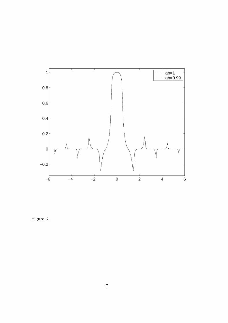
In Fig. 2 we show h3;� and ah3;� for � =p2� and a = b =

p0:9, and in

Fig. 3 we show h3;� and ah3;� for � =p2� and a = b =

p0:99. The h3;�

was obtained from (8) while the ah3;�'s were obtained using the algorithm to

compute S�1=2a h as can be found in [8], Sec. 4.

4 Even, positive windows with one Zak trans-

form zero

In this section we consider general even, positive continuous windows g withsuÆcient decay so that Zg is a continuous function on R2 . We are particularly

interested here in windows g such that Zg has a single zero in [0; 1)2, which

then must occur at (12; 12). A class of windows g having all these properties

was studied in [5], Sec. 2. The windows g considered there are even and

continuous, and have on [0;1) the form

g(t) = b(t) + b(t+ 1) ; t � 0 ; (39)

with b integrable, non-negative and strictly convex on [0;1). The latter con-

dition is referred to as super convexity in [5]. A disadvantage of this class isthat it is not dilation invariant because of the occurrence of the shift-by-oneoperation in (39). A class of windows that is dilation invariant and whose

members are super convex with an arbitrary shift operator b ! (b � + �)

in (39) is considered in [5], Subsec. 2.4.4: g even, integrable and continuous

10

with (�1)n g(n)(t) > 0 for t � 0, n = 0; 1; 2; 3.

Symmetry properties and the Zak transform. Let g : R ! C be

continuous and (rapidly) decaying so that we can consider Z = Zg in a

pointwise manner. There hold the quasi-periodicity relations

Z(t + 1; �) = e2�i� Z(t; �) ; Z(t; � + 1) = Z(t; �) ; t; � 2 R : (40)

There holds furthermore

g real, Z�(t; �) = Z(t;��) ; t; � 2 R ; (41)

g even, Z(t; �) = Z(�t;��) ; t; � 2 R : (42)

From the quasi-periodicity relations in (40) and (41), (42) one gets the fol-

lowing further properties of Z when g is real and even:

Z(1� t; �) = e2�i� Z(�t; �) = e2�i� Z�(t; �) ; (43)

Z(t; 1� �) = Z(t;��) = Z�(t; �) = Z(�t; �) ; (44)

e��i� Z(12; �) = e�i� Z�(1

2; �) 2 R ; (45)

Z(t; 0) 2 R ; Z(t; 12) = �Z(1� t; 1

2) 2 R ; (46)

e��i� Z(12; �) = �e��i(1��) Z(1

2; 1� �) ; (47)

Z(0; �) = Z(1; �) e�2�i� 2 R ; (48)

Z(12; 12) = 0 ; (49)

where t; � 2 R.

We next consider for real and even windows g with single zero of Zg in

[0; 1)2 at (12; 12) the tight frame generating h = Z�1(Zg=jZgj) that is given

explicitly by (I any interval of length 1)

h(t) =ZI

(Zg)(t; �)

j(Zg)(t; �)j d� ; t 2 R : (50)

We collect the following obvious properties of h.

Proposition 4.1. We have

(a) h is real and even,

(b) h is continuous,

11

(c) h is bounded: jh(t)j � 1, t 2 R.

Proof. Note that Zh = Zg=jZgj. Then(a) follows from the equivalences in (41), (42),

(b) follows from continuity of Zg and the fact that Zg has just one zero

per unit square,

(c) follows trivially from (50).

The following result is slightly less obvious.

Proposition 4.2. Assume that g(t) > 0, t 2 R. Then we have

h(n) = Æn ; h(n+ 12) =

(�1)n�(n+ 1

2); (51)

where Æn denotes Kronecker's delta.

Proof. We have for t 2 [0; 1), n 2 Z by the �rst relation in (40)

h(n + t) =ZI

(Zh)(n+ t; �) d� =ZI

(Zg)(t; �)

j(Zg)(t; �)j e2�in� d� : (52)

Since (Zg)(0; �) is real, 6= 0 (as Zg vanishes only at (12; 12) in [0; 1)2) and

(Zg)(0; 0) > 0, we have that (Zg)(0; �) > 0 for � 2 R. Consequently,

(Zg)(0; �)=j(Zg)(0; �)j = 1 for � 2 R and it follows at once that h(n) = Æn,n 2 Z.

Next we have from (45) that exp(��i�)(Zg)(12; �) is real, 6= 0, when

� 2 [0; 1), � 6= 12. Moreover, by (47) we see that exp(��i�)(Zg)(1

2; �) is

positive for 0 � � < 12and negative for 1

2< � � 1. Hence

h(n + 12) =

1Z0

(Zg)(12; �)

j(Zg)(12; �)j e

2�in� d� =

=

1Z0

(Zg)(12; �) e��i�

j(Zg)(12; �) e��i�j e

2�i(n+12)� d� =

=

1Z0

sgn(12� �) e2�i(n+

12)� d� =

(�1)n�(n+ 1

2); (53)

as claimed.

12

We next give an inequality for h(t), t 2 [0; 1).

Proposition 4.3. We have

h(t) + h(1� t) � 4

�; t 2 [0; 1) : (54)

Proof. There holds by (43) for any t 2 [0; 1)

h(t) + h(1� t) =

1=2Z�1=2

(Zg)(t; �) + e2�i�(Zg)�(t; �)

j(Zg)(t; �)j d� =

= 2

1=2Z�1=2

Re(e��i�(Zg)(t; �))

j(Zg)(t; �)j e�i� d� : (55)

Since h(t) + h(1 � t) is real we can take the real part of (55). Then the

inequality follows from the fact that

cos �� � 0 ;Re(e��i�(Zg)(t; �))

j(Zg)(t; �)j � 1 ; � 12� � � 1

2; (56)

and

1=2Z�1=2

cos �� d� = 2=�.

Note. For g super convex there is also the inequality h(t) + h(1 � t) � 0,

t 2 [0; 1); this requires a rather delicate analysis of the Zak transforms of

super convex functions, compare [5], Subsec. 2.2. In Sec. 6 this latter in-equality will be strengthened to h(t) + h(1 � t) � 1, t 2 [0; 1), for the case

that g = g3;�.

We conclude this section by showing that, under some further conditions

on g, the h of (50) is in L1(R). These conditions are that Zg is smooth on[0; 1)2 and that there are real A 6= 0 6= B such that (as (t; �)! (1

2; 12))

(Zg)(t; �) = A(t� 12) + iB(� � 1

2) +O((t� 1

2)2 + (� � 1

2)2) : (57)

Observe that

A =@ Zg

@t(12; 12) = 2

1Xk=0

(�1)k g0(k + 12) ;

B =1

i

@ Zg

@�(12; 12) = �2�

1Xk=0

(�1)k(2k + 1) g(k + 12) :

(58)

13

Theorem 4.1. Under the above conditions on g we have

1Xn=�1

jh(t+ n)j = O(jt� 12j�1=2) ; t 2 [0; 1) : (59)

In particular we have that h 2 L1(R).

Proof. We have for t 2 [0; 1), t 6= 12by partial integration

h(t + n) =

1Z0

e2�in�(Zh)(t; �) d� =

=�12�in

1Z0

@ Zh

@�(t; �) e2�in� d� ; n 2 Z : (60)

Hence by the Cauchy-Schwarz inequality and Parseval's theorem for Fourier

series

Xn6=0

jh(t+ n)j ��Xn6=0

1

4�2n2

�1=2�Xn6=0

���1Z

0

@Zh

@�(t; �) e2�in� d�

���2�1=2 �

�� 1

12

1Z0

���@ Zh@�

(t; �)���2 d��1=2 : (61)

We shall estimate

I(t) :=

1Z0

���@ Zh@�

(t; �)���2 d� : (62)

We have for (t; �) 6= (12; 12) from Zh = Zg=jZgj that

@ Zh

@�=

@ Zg

@�jZgj �

@

@�jZgj

(Zg)�: (63)

Furthermore there holds for (t; �) 6= (12; 12)

@

@�j(Zg)(t; �)j �

���@ Zg@�

(t; �)��� : (64)

Now by the assumptions on Zg, see (57), there are " > 0, Æ > 0 such that

j(Zg)(t; �)j � (12A2(t� 1

2)2 + 1

2B2(� � 1

2)2)1=2 (65)

14

when jt � 12j � ", j� � 1

2j � Æ. Moreover, since Zg only vanishes at (1

2; 12)

within [0; 1)2 there is a c > 0 such that

j(Zg)(t; �)j � c (66)

when jt� 12j � " or j�� 1

2j � Æ. Next letting C be an upper bound for

���@ Zg@�

���we conclude that

���@ Zh@�

(t; �)��� � 2C(1

2A2(t� 1

2)2 + 1

2B2(� � 1

2)2)�1=2 (67)

when jt� 12j � ", j� � 1

2j � Æ, and that

���@ Zh@�

(t; �)��� � 2C=c (68)

when jt� 12j � " or j� � 1

2j � Æ. We conclude from (67), (68) that

I(t) � 4C2=c2 ; jt� 12j � " ; (69)

and that

I(t) � (1�2Æ) 4C2=c2+

12+ÆZ

12�Æ

8C2

A2(t� 12)2 +B2(� � 1

2)2d� ; jt� 1

2j � " : (70)

Finally

12+ÆZ

12�Æ

d�

A2(t� 12)2 +B2(� � 1

2)2� 2

1Z0

d�

A2(t� 12)2 +B2�2

=�

ABjt� 12j ; (71)

and the proof is complete.

Note. We observe that the condition A 2 R, B 2 R, A 6= 0 6= B, see

(57), is satis�ed by g = g1; ; g2; ; g3;�, see (36){ (38). In Sec. 6 we shall

improve Thm. 4.1 for the case that g = g3;�.

5 Two-sided exponentials yield Gabor frames

In this section we show that (g3;�; a; b) is a Gabor frame when a > 0, b > 0,ab < 1 and � > 0. For the proof we follow largely the approach in [6],

15

Sec. 2, where it was shown that (g2; ; a; b) is a Gabor frame when a > 0,

b > 0, ab < 1 and > 0. Accordingly, by scale invariance of the class of

two-sided exponentials and the fact that (g; a; b) is a frame if and only if

(c1=2 g(c�); a=c; bc) is a frame (any c > 0), we can assume that b = 1, a < 1.

We thus consider the Ron-Shen matrices, see [4], Sec. 7.4,

(g3;�(t� na� l))l2Z;n2Z ; (72)

and we should show that there are A > 0, B <1 such that

A kck2 �1X

n=�1

��� 1Xl=�1

cl g(t� na� l)���2 � B kck2 (73)

for all t 2 R and all c 2 l2(Z). When A > 0 and B < 1 as in (73) exist,

they are a lower and upper frame bound, respectively, for the Gabor system

(g3;�; a; 1). Evidently, by exponential decay of g, we do not need to worryabout the existence of a �nite B such that the right inequality in (73) holdsfor all t 2 R, c 2 l2(Z), and so we concentrate on the left inequality.

We write, see [6], Sec. 2, for c 2 l2(Z), t 2 R, n 2 Z

Xl

cl g3;�(t� na� l) =

1Z0

(Zg3;�)(t� na; �)C�(�) d� =

=

1Z0

e2�ibt�nac�(Zg3;�)(ht� nai; �)C�(�) d�;(74)

where for x 2 R

bxc = largest integer � x ; hxi = x� bxc ; (75)

andC(�) =

Xl

c�l e2�il� ; a:e: � 2 R : (76)

In (74) the quasi-periodicity relations in (40) have been used.

To proceed we need to calculate Zg3;�.

Proposition 5.1. We have for (t; �) 2 [0; 1)2

(Zg3;�)(t; �) = (r2(t) + r1(t) e2�i�) �(�) ; (77)

where

�(�) =2�1=2 e��

1� 2e�� cos 2�� + e�2�; r1(t) = r2(1� t) = sinh�t : (78)

16

Proof. Let t 2 [0; 1), � 2 R. Then

(Zg3;�)(t; �) =1X

k=�1

�1=2 e��jt�kj e2�ik� =

= �1=2 e��(1�t) � e2�i�

1� e�� e2�i�+ �1=2 e��t � 1

1� e�� e�2�i�; (79)

where the second identity in (79) follows from splitting up the summation

range of the �rst line series into k � 1 (so that t� k > 0) and k � 0 (so that

t � k � 0) and summing the two geometric series. Then (77){(78) follows

easily.

We conclude from (74) and Proposition 5.1 that for c 2 l2(Z), t 2 R,

n 2 ZXl

cl g3;�(t� na� l) = r2(ht� nai) dbt�nac + r1(ht� nai) dbt�nac+1 ; (80)

when the dk's are de�ned by

�(�)C(�) =Xk

d�k e2�ik� ; a:e: � 2 R : (81)

Note that by Parseval's formula for Fourier series we have

m kck � kdk �M kck ; (82)

where m > 0, M < 1 are the minimum and maximum of �, and c and d

are related to one another according to (76), (81).We can express (80) in the formX

l

cl g3;�(t� na� l) = (R(t)d)n ; (83)

where R(t) is the linear operator of l2(Z) given by its matrix elements with

respect to the standard basis of l2(Z) as

Rnk(t) =

8>>>><>>>>:

r2(ht� nai) ; k = bt� nac

r1(ht� nai) ; k = bt� nac + 1

0 ; otherwise ;

(84)

with n the row index and k the column index. On account of (82) we shouldthus show that there is a K > 0 such that

kR(t)dk2 =1X

n=�1

j(R(t)d)nj2 � K kdk2 (85)

17

for all t 2 R, d 2 l2(Z).We distinguish now between the cases that a � 1

2and a > 1

2.

Case a � 12. Take t 2 R. For any k 2 Z there are at least two consec-

utive n 2 Z such that k = bt � nac; denote the largest, smallest such n by

nk;+, nk;�. Evidently

kR(t)dk2 �1X

k=�1

fj(R(t)d)nk;+j2 + j(R(t)d)nk;�

j2g : (86)

We can write for k 2 Z

j(R(t)d)nk;+ja + j(R(t)d)nk;�

j2 = 24 r2(s1) r1(s1)

r2(s2) r1(s2)

3524 dk

dk+1

35 2

; (87)

where s1, s2 are numbers satisfying 0 � s1 � s2� 12< 1

2. A plot or r1(s) and

r2(s), s 2 [0; 1], suÆces to see that there is a constant C > 0 such that forall v = [v1 v2]

T 2 C2 and all s1, s2 with 0 � s1 � s2 � 1

2< 1

2we have

24 r2(s1) r1(s1)

r2(s2) r1(s2)

3524 v1

v2

35 2

� C kvk2 = C(jv1j2 + jv2j2) : (88)

Hence we see that

kR(t)dk2 � C1X

k=�1

(jdkj2 + jdk+1j2) = 2C kdk2 ; (89)

and this completes the proof for the case a � 12.

Case a 2 (m=(m + 1); (m + 1)=(m + 2)], m = 1; 2; ::: . Let t 2 R. Weorder the set of n 2 Z such that bt � nac = bt� (n + 1) ac as an increasing

sequence (nj)j2Z, where we observe that for all j 2 Z

m+ 1 � nj+1 � nj � m + 2 : (90)

Next we write

kR(t)dk2 =1X

n=�1

j(R(t)d)nj2 =

=1X

j=�1

n12j(R(t)d)nj

j2 + 12j(R(t)d)nj+1j2 +

Xnj<n<nj+1

j(R(t)d)nj2 +

+ 12j(R(t)d)nj+1

j2 + 12j(R(t)d)nj+1+1j2

o: (91)

18

That is

kR(t)dk2 =1X

j=�1

kR(j)(t)d(j)k2 ; (92)

where d(j) is the subvector of d made up from the consecutive entries dk of d

with index k = bt� njac; :::; bt� nj+1ac+ 1, and R(j)(t) is the submatrix of

R(t) made up from the entries Rnk(t) of R(t) with row index n = nj; :::; nj+1+

1 and column index k = bt� njac; :::; bt� nj+1ac+1, where the entries with

row index n = nj; nj + 1; nj+1; nj+1 + 1 are divided byp2.

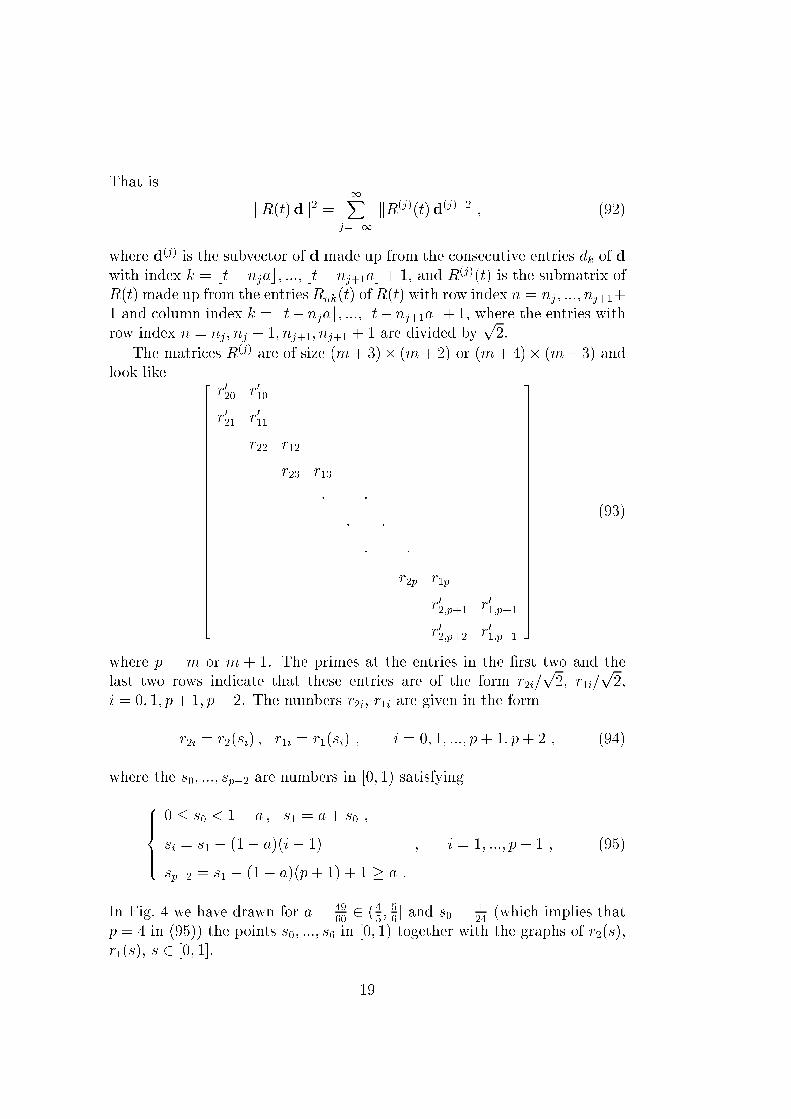
The matrices R(j) are of size (m+ 3)� (m+2) or (m+4)� (m+3) and

look like 2666666666666666666666666664

r020 r010

r021 r011

r22 r12

r23 r13

� �� �� �

r2p r1p

r02;p+1 r01;p+1

r02;p+2 r01;p+1

3777777777777777777777777775

(93)

where p = m or m + 1. The primes at the entries in the �rst two and thelast two rows indicate that these entries are of the form r2i=

p2, r1i=

p2,

i = 0; 1; p+ 1; p+ 2. The numbers r2i, r1i are given in the form

r2i = r2(si) ; r1i = r1(si) ; i = 0; 1; :::; p+ 1; p+ 2 ; (94)

where the s0; :::; sp+2 are numbers in [0; 1) satisfying

8>>><>>>:

0 � s0 < 1� a ; s1 = a+ s0 ;

si = s1 � (1� a)(i� 1) ; i = 1; :::; p+ 1 ;

sp+2 = s1 � (1� a)(p+ 1) + 1 � a :

(95)

In Fig. 4 we have drawn for a = 49602 (4

5; 56] and s0 =

124

(which implies that

p = 4 in (95)) the points s0; :::; s6 in [0; 1) together with the graphs of r2(s),

r1(s), s 2 [0; 1].

19

The 2� 2-matrices24 r020 r010

r021 r011

35 ;

24 r02;p+1 r01;p+1

r02;p+2 r01;p+2

35 (96)

are, except for the factors 1=p2, of a similar type as the 2 � 2-matrix oc-

curring at the right-hand side of (87). Hence they satisfy an inequality of

the type (88) with a constant C > 0 which is independent of the particular

con�guration s0; :::; sp+2 as in (95). We next consider the submatrix of (93)

obtained by deleting the �rst and last column and the �rst 2 and last 2 rows,

and write it in the form2666666666666666666666664

a1 b1a2 b2

� �� �

� �ak bk

ak+1 bk+1

� �� �

� �aK�1 bK�1

aK bK

3777777777777777777777775

;

(97)

where K = p� 1 and k is to be speci�ed below. The matrix in (97) has two

non-zero diagonals where the lower diagonal entries increase from a valuea1 = r22 < r12 = b2 to a value aK = r2p > r1p = bK while the upper diagonal

entries decrease from a value b1 = r12 > r22 = a1 to a value bK = r1p < r2p =

aK. We take k such that ak � bk, ak+1 � bk+1. Then

a1 < a2 < ::: < ak � bk < bk�1 < ::: < b2 < b1 ; (98)

bK < bK�1 < ::: < bk+1 � ak+1 < ak+2 < ::: < aK�1 < aK : (99)

Accordingly there holds for any x = [x1; :::; xK+1]T 2 C

K+1

KXi=1

jaixi + bixi+1j �KXi=1

(bi jxi+1j � ai jxij) +KX

i=k+1

(ai jxij � bi jxi+1j) =

= �a1 jx1j+kX

i=2

(bi�1 � ai) jxij+ bk jxk+1j +

20

� bK jxK+1j+KX

i=k+2

(ai � bi�1) jxij+ ak+1 jxk+1j : (100)

Now suppose that we have a vector e = [e0; :::; ep+1] 2 Cp+2 such that

kR(j)(t) ek2 =p+2Xi=0

j(R(j)(t) e)ij2 � 1 : (101)

The considerations of the matrices in (96) yield that there is a constant C

(only depending on �, a) such that

je0j; je1j; jepj; jep+1j � C : (102)

Next, also see Fig. 4 and (93), (94), (97), there is a Æ > 0, only dependingon � and a, such that

bi�1 � ai � Æ ; i = 2; :::; k ; ai � bi�1 � Æ ; i = k + 2; :::; K ; (103)

while also bk � Æ, ak+1 � Æ. Therefore

pXi=2

j(R(j)(t) e)ij � Æp�1Xi=2

jeij � r22je1j � r1pjepj : (104)

It thus follows from (101), (102) that

p�1Xi=2

jeij �1

Æ(2MC +

qp� 1) ; (105)

where M = max(r22; r1p) � sinh(�=2). Hence

kek2 =p+1Xi=0

jeij2 �� pXi=0

jeij�2� (4C + �1(2MC +

qp� 1))2 : (106)

We thus conclude that there is a constant D > 0, only depending on � and

a, such that

kR(j)(t) ek2 � D kek2 ; t 2 R ; e 2 Cp+1 ; j 2 Z : (107)

This implies that there is a constant D > 0 such that for t 2 R, d 2 l2(Z)

kR(t)dk2 =1X

j=�1

kR(j)(t)d(j)k2 � D1X

j=�1

kd(j)k2 � D kdk2 ; (108)

21

and this completes the proof for the case a 2 (m=(m+ 1); (m+ 1)=(m+ 2)].

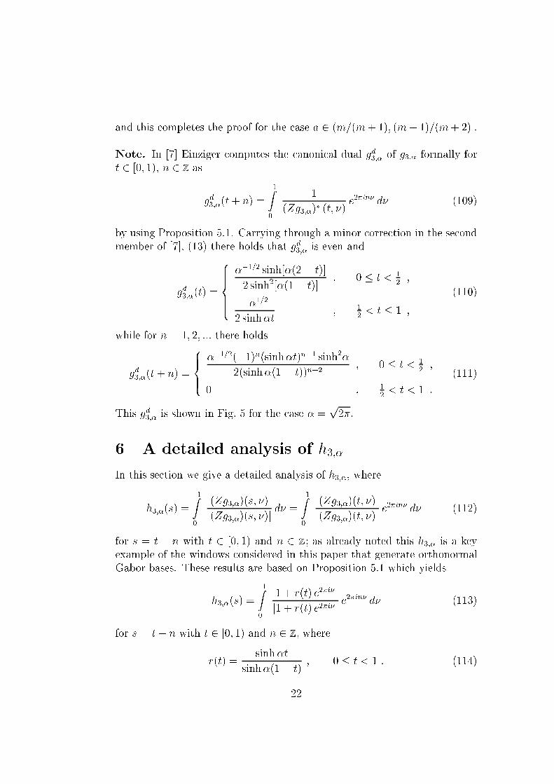
Note. In [7] Einziger computes the canonical dual gd3;� of g3;� formally for

t 2 [0; 1), n 2 Z as

gd3;�(t+ n) =

1Z0

1

(Zg3;�)� (t; �)e2�in� d� (109)

by using Proposition 5.1. Carrying through a minor correction in the second

member of [7], (13) there holds that gd3;� is even and

gd3;�(t) =

8>>>><>>>>:

��1=2 sinh[�(2� t)]

2 sinh2[�(1� t)]; 0 � t < 1

2;

��1=2

2 sinh�t; 1

2< t � 1 ;

(110)

while for n = 1; 2; ::: there holds

gd3;�(t+ n) =

8>><>>:��1=2(�1)n(sinh�t)n�1 sinh2�

2(sinh�(1� t))n+2; 0 � t < 1

2;

0 ; 12< t < 1 :

(111)

This gd3;� is shown in Fig. 5 for the case � =p2�.

6 A detailed analysis of h3;�

In this section we give a detailed analysis of h3;�, where

h3;�(s) =

1Z0

(Zg3;�)(s; �)

j(Zg3;�)(s; �)jd� =

1Z0

(Zg3;�)(t; �)

j(Zg3;�)(t; �)je2�in� d� (112)

for s = t + n with t 2 [0; 1) and n 2 Z; as already noted this h3;� is a key

example of the windows considered in this paper that generate orthonormal

Gabor bases. These results are based on Proposition 5.1 which yields

h3;�(s) =

1Z0

1 + r(t) e2�i�

j1 + r(t) e2�i�j e2�in� d� (113)

for s = t+ n with t 2 [0; 1) and n 2 Z, where

r(t) =sinh�t

sinh�(1� t); 0 � t < 1 : (114)

22

Since h3;� is even it is therefore suÆcient to consider for n = 0; 1; ::: the

integrals

In(r) =

1Z0

1 + r e2�i�

j1 + r e2�i� j e2�in� d� ; r � 0 : (115)

A. Representations of In(r)

In this subsection we present a number of representations of In(r). We let

for r � 0

k2 :=4r

(1 + r)2=

4r�1

(1 + r�1)22 [0; 1] : (116)

A.1. Representation in terms of elliptic integrals

We have

In(r) =2

�(1 + r)(Kn(k

2) + rKn+1(k2)) ; (117)

where

Kn(k2) =

�=2Z0

cos 2nxp1� k2 sin2 x

dx ; n = 0; 1; ::: : (118)

For n = 0 there holds speci�cally

I0(r) =1

�(1� r)K(k2) +

1

�(1 + r)E(k2) ; (119)

with

K(k2) =

�=2Z0

(1�k2 sin2 x)�1=2 dx ; E(k2) =

�=2Z0

(1�k2 sin2 x)1=2 dx (120)

the complete elliptic integrals of the �rst and second kind, respectively, see

[9], p. 590, for m = k2 < 1. The proof of these results is elementary.From [10], 806.01 on p. 292 we have for Kn the series representation

Kn(k2) = (�1)n �

2

1Xj=n

� 2jj

� � 2j

j � n

�(14k)2j : (121)

Accordingly we get for In(r) the series representation

In(r) =(�1)n1 + r

1Xj=n

� 2jj

� � 2j

j � n

�(14k)2j

n1� rk2

(j + 12)2

(j + n+ 1)(j + n+ 2)

o:

(122)

23

While the series in (121) only converges for 0 � k2 < 1, the series in (122)

converges for k2 = 1 as well by Stirling's formula and the fact that the factor

in f g is O(j�1).

A.2. Integral representations of In(r)

Aside from the direct representation of In(r) through the de�nition (115),

we have the integral representations for n = 0; 1; :::, r > 0

In(r) =(�1)n�

min(r;r�1)Z0

vn�1=2s1� rv

r � vdv =

= (�1)n1=2Z

�1=2

Rn(�)1 +R(�)

1 + r

1� r R(�)

1� R(�)d� : (123)

Here R(�) = R(r ; �) is for r � 0 and � 2 [�12; 12] the unique solution

R 2 [0; 1] of the equation

4R

(1 +R)2=

4r

(1 + r)2cos2 2�� : (124)

Note that R(�) � min(r; 1=r), whence the second integrand in (123) isbounded since

0 � 1� r R(�)

1�R(�)� 1+ r ; 0 � r < 1 ; 0 � 1� r R(�)

1� R(�)� 1 ; 1 � r <1 :

(125)

The �rst integrand in (123) has for 0 < r < 1 a (r � v)�1=2-behaviour when

v " r.

Proof of the �rst representation in (123). Consider the case that0 < r � 1. Letting z = e2�i� in the right-hand side of (115), we have

In(r) =1

2�i

Zjzj=1

1 + rz

j1 + rzj zn�1 dz : (126)

On jzj = 1 we have

j1 + rzj =q(1 + rz)(1 + rz�1) (127)

when we choose the principal square root. The right-hand side of (127)

is analytic in the whole complex plane, except for the branch cuts [�r; 0],

24

(�1;�1=r]. From a consideration of the right-hand side of (127) near z = 0,

Im z 6= 0 it follows thatq(1 + r(�v � i0))(1 + r(�v � i0)�1) = � i

q(1� rv)(rv�1 � 1) ;

0 � v � r ; (128)

with a non-negative square root at the right-hand side of (128). Now de-

forming the integration contour jzj = 1 in (126) into a contour tightly �tting

around the branch cut [�r; 0] we get the �rst representation in (123) for

0 < r � 1 by Cauchy's theorem.

We observe that

limr#0

rZ0

vn�1=2s1� rv

r � vdv = � Æno ; n = 0; 1; ::: ; (129)

where Æno is Kronecker's delta, which is consistent with (115) for r = 0.

The case that r � 1 is handled in a similar manner, except that thebranch cuts for (127) are now [�1=r; 0], (�1;�r].

Proof of the second representation in (123). We have from (117),(121) when r 6= 1

(�1)n(1 + r) In(r) =1Xj=n

1

4j

� 2jj

� � 2j

j � n

�(14k2)j +

� 14rk2

1Xj=n

1

4j+1

� 2j + 2

j + 1

� � 2j + 2

j � n

�(14k2)j : (130)

Using that

1

4m

� 2mm

�=

1=2Z�1=2

(cos2 2��)m d� ; m = 0; 1; ::: ; (131)

we get

(�1)n(1 + r) In(r) =

1=2Z�1=2

n 1Xj=n

� 2j

j � n

�(14k2 cos2 2��)j +

� 14rk2 cos2 2��

1Xj=n

� 2j + 2

j � n

�(14k2 cos2 2��)j

od� : (132)

25

Next we use [11], 5.2.13.29 on p. 713 with � = 2n+ 1 and 2n+ 3, v = 2 and

x = 14k2 cos2 2�� 2 [0; 1

4], so that

1Xj=n

� 2j

j � n

�xj = xn

y2n+1

�y + 2;

1Xj=n

� 2j + 2

j � n

�xj = xn

y2n+3

�y + 2; (133)

where x 2 [0; 14] and y 2 [1; 2] are related according to

x =y � 1

y2: (134)

Recalling the de�nitions (124) of R(�), (116) of k2 and x = 14k2 cos2 2��,

we easily see that

y(�) = y = 1 +R(�) ; R(�) = 14k2y2 cos2 2�� : (135)

Using this in (132) we obtain

(�1)n(1 + r) In(r) =

1=2Z�1=2

Rn(�) y(�)

�y(�) + 2(1� r R(�)) d� =

=

1=2Z�1=2

Rn(�)(1 +R(�))1� r R(�)

1� R(�)d� ; (136)

as required.

The second representation in (123) can also be written as

In(r) = 4(�1)n1=4Z0

Rn(�)1 +R(�)

1� R(�)

1� r R(�)

1 + rd� ; (137)

and this yields the �rst representation in (123) by the substitution v =

R(�) 2 [0;min r; 1=r], � 2 [0; 14]. To see this we set

V =

ssin2 2��+

�1� r

1 + r

�2cos2 2�� : (138)

Then we �nd from (124) and 0 � R(�) � 1 that

1 +R(�)

1� R(�)=

1

V; R(�) =

1� V

1 + V=

4r cos2 2��

(1 + r)2

� 1

1 + V

�2; (139)

26

R0(�) =�16�r sin 2��cos 2��

(1 + r)2 V (1 + V )2; (140)

so that1 +R(�)

1�R(�)=�14�

cos 2��

sin 2��

R0(�)

R(�): (141)

Furthermore, one has

(r �R(�))(1� r R(�)) = (1 + r)2R(�)sin2 2��

cos2 2��; (142)

so that for � 2 [0; 14]

1� r R(�) = (1 + r)R1=2(�)sin 2��

cos 2��

vuut1� r R(�)

r � R(�): (143)

When one uses (141) and (143) in the right-hand side of (137) one gets the�rst representation in (123) by setting v = R(�).

B. Consequences of the representations

We shall now give a number of consequences of the representations of In(r)

obtained in A. These consequences translate directly to properties of h3;�since h3;�(t+n) = In(r(t)) for t 2 [0; 1), n = 0; 1; ::: with r(t) given in (114).

B.1. Behaviour of h3;� at the integers and half-integers

It is clear that h3;� is a smooth function away from the integers and the

half-integers. From Prop. 4.1 (b) we know that h is continuous everywhere.

To study the behaviour of h3;� at the integers, we note that for n = 1; 2; :::

and t 2 [0; 1) there holds

h3;�(n + t) = In(r) ; h3;�(n� t) = In�1(1=r) (144)

with r = r(t), see (114). Thus we shall compare the behaviour of In(r),In(1=r) as r # 0 for n = 1; 2; ::: . For n = 0 we have the special situation thath3;�(t) = h3;�(�t), whence we only have to consider I0(r) as r # 0.

Proposition 6.1. We have

(a) I0(r) has a convergent power series in r 2 C for jrj < 1 with only even

powers of r, and I0(0) = 1,

27

(b) In(r) and In�1(1=r) have for n = 1; 2; ::: a convergent power series in

r 2 C for jrj < 1, and there holds

In(r) = (�1)n� 2nn

� �r4

�n+O(rn+1) ;

In�1(1=r) = (�1)n�1 n

2n� 1

� 2nn

� �r4

�n+O(rn+1) (145)

as r # 0.

Proof. We have for 0 � r < 1 that

I0(r) = 2

1=2Z0

1 + r cos 2��

(1 + r2 + 2r cos 2��)1=2d� : (146)

It is not diÆcult to see that for any a 2 [�1; 1] the image of z 2 C , jzj < 1under the mapping z ! 1+ z2+2za and the set (�1; 0] are disjoint. Hencethe right-hand side of (146) extends to an analytic function of r 2 C , jrj < 1

when we take the principal square root for (1 + r2 + 2r cos 2��)1=2 wherejrj < 1, � 2 [0; 1

2]. Thus I0(r) has a convergent power series in r 2 C , jrj < 1.

Furthermore, we have

1=2Z0

1� r cos 2��

(1 + r2 � 2r cos 2��)1=2d� =

1=2Z0

1 + r cos 2��

(1 + r2 + 2r cos 2��)1=2d� ; (147)

as we see by replacing � by 12� � in the left-hand side integral in (147). It

follows that the right-hand side of (146) is an even function of r, jrj < 1.Evidently, I0(0) = 1 and this completes the proof of (a).

As to (b) we start by noting that

In(r) =

1=2Z�1=2

1 + r e2�i�

(1 + r2 + 2r cos 2��)1=2e2�in� d� ; (148)

In�1(1=r) =

1=2Z�1=2

1 + r e�2�i�

(1 + r2 + 2r cos 2��)1=2e2�in� d� ; (149)

and the statement about the convergent power series follows in a similar

manner as in (a). The formulas in (145) are an easy consequence of the se-

ries representation in (122), also see (116).

28

Note. We have that

limr#0

r�n In(r) 6= (�1)n limr#0

r�n In�1(1=r) (150)

unless n = 1 in which case the two members of (150) equal �1=2.

As a consequence we have that h3;� is analytic at t = 0, that h3;� is

di�erentiable at t = n = 1 (with derivative equal to ��=2 sinh�), and that

h3;� has zeros of order n with non-zero, unequal left and right derivatives of

order n at t = n = 2; 3; ::: .

We next consider the behaviour of h3;� at the half-integers t = n + 12,

n = 0; 1; ::: . Since r(12) = 1 we thus need to consider In around r = 1.

Proposition 6.2. We have (�1)n+1 I 0n(1) = +1 for n = 0; 1; ::: .

Proof. We consider the �rst representation of In(r) in (123). It suÆces for

our purposes to study the functions

rZ0

s1� rv

r � vdv ;

sZ0

ss� v

1� svdv (151)

as r " 1 and s = (1=r) " 1, since the function v ! vn�1=2 is smooth at v = 1.We compute, explicitly,

rZ0

s1� rv

r � vdv =

1

2prf2r + (1� r2) ln(1 + r)� (1� r2) ln(1� r)g ; (152)

sZ0

ss� v

1� svdv =

1

2spsf2s� (1� s2) ln(1 + s) + (1� s2) ln(1� s)g : (153)

Now it is evident that the terms �(1 � r2) ln(1 � r) and (1 � s2) ln(1 � s)

cause the derivatives of the left-hand sides of (152) and (153) at r = 1 and

s = 1 to be �1 and +1, respectively. This proves the result.

B.2. Special values

We have

K(k2) = 12� F (1

2; 12; 1 ; k2) ; E(k2) = 1

2� F (�1

2; 12; 1 ; k2) ; (154)

29

with F a hypergeometric function, see [9], 17.3.9{10 on p. 591 and Ch. 15. A

special value of K, E occurs when k2 = 12, i.e. r = 3� 2

p2, see [9], 15.1.25{

26, cases a = 12, b = 1 and a = � 1

2, b = 1

2, on p. 557. Thus

F (12; 12; 1 ; 1

2) =

�1=2

�2(34); F (�1

2; 12; 1 ; 1

2) = 2�1=2

� 1

4�2(34)+

1

�2(14)

�: (155)

Then (119) yields

I0(3� 2p2) =

(�=2)1=2

�2(34)

+�2(3

4)

�3=2(2�

p2) = 0:992599562 ; (156)

I0(3 + 2p2) = � (�=2)1=2

�2(34)

+�2(3

4)

�3=2(2 +

p2) = 0:08610564 : (157)

B.3. Positivity and monotonicity of (�1)n In(r)

We have the following result.

Theorem 6.1. There holds

(a) I0(r) is positive and decreasing in r � 0,

(b) (�1)n In(r) is positive for r > 0 and decreasing in r � 1.

Proof. (a) We have from (115) that

I0(r) = 2

1=2Z0

J(r; �)

(J2(r; �) +K2(r; �))1=2d� ; r � 0 ; (158)

where

J(r; �) = 1+ r cos 2�� ; K(r; �) = r sin 2�� ; r � 0 ; 0 � � � 12: (159)

Fix � 2 (0; 12). Then K(r; �) > 0 for r > 0 while

J(r; �)

K(r; �)=

1

r sin 2��+ cotg 2�� (160)

decreases in r > 0. Then one easily sees that

J(r; �)

(J2(r; �) +K2(r; �))1=2=

sgn(J(r; �))

(1 +K2(r; �)=J2(r; �))1=2(161)

30

decreases in r > 0. Since I0(0) = 1, I0(1) = 0, the proof of (a) is complete.

(b) That (�1)n In(r) > 0 for r > 0 follows at once from either represen-

tation in (123). Next we have for r � 1 by the �rst representation in (123)

that

(�1)n In(r) =1

�

1=rZ0

vn�1=2s1� rv

r � vdv =

=1

�

1Z0

vn�1=2s1� rv

r � v�[0;1=r)(v) dv : (162)

One easily sees that the integrand in the integral on the second line of (162)

decreases in r � 1 for any v � 0. This proves (b).

B.4. An inequality

We have the following counterpart of Prop. 4.3 for h3;�.

Proposition 6.3. With R(r;�) = R(�) as de�ned through (124) we have

I0(r) + I0(1=r) =

1=2Z�1=2

(1 +R(r;�)) d� � 1 ; 0 � r <1 : (163)

Proof. Taking 0 � r � 1 we have from the second representation in (123)for n = 0 that

I0(r) + I0(1=r) =

1=2Z�1=2

1 +R(r;�)

1 + r

1� r R(r;�)

1�R(r;�)d� +

+

1=2Z�1=2

1 +R(r;�)

1 + 1=r

1� R(r;�)=r

1� R(r;�)d� =

=

1=2Z�1=2

(1 +R(r;�)) d� : (164)

Since R(r;�) � 0 we see that the right-hand side of (164) � 1, and this

completes the proof.

31

Improvements of the inequality in (163), as well as inequalities with �instead of �, are obtained easily from the explicit forms (138), (139). We do

not elaborate this point here.

B.5. Sharper form of Theorem 4.1.

We have the following sharper form of Theorem 4.1 for h = h3;�.

Theorem 6.2. We have

1Xn=0

jh3;�(t+ n)j = O(ln jt� 12j�1) ; t! 1

2: (165)

Proof. With r = r(t), see (114), we have from Theorem 6.1 (a) and the

second representation in (123) that

1Xn=0

jh3;�(t+ n)j =1Xn=0

(�1)n In(r) =4

1 + r

1=4Z0

1 +R(�)

1� R(�)

1� r R(�)

1�R(�)d� :

(166)

By (138), (139) we have that

4

1=4Z0

1 +R(�)

1� R(�)d� = 4

1=4Z0

�sin2 2��+

�1� r

1 + r

�2cos2 2��

��1=2d� =

=2

�

�=2Z0

dxp1� k2 sin2 x

=2

�K(k2) ; (167)

with k2 as in (116). Also, by [9], 17.3.26 on p. 591 we have

K(k2) = ln 4���1 + r

1� r

���+ o(1) ; r ! 1 : (168)

Finally, by (125), we have that (1� r R(�))=(1�R(�)) is bounded between0 and 2 for all r � 0 and all � 2 [0; 1

4). Then the result follows on combining

(166), (167), (168).

B.6. Inequality for (�1)n In(r)

We have the following inequality for (�1)n In(r), r � 0, n = 0; 1; ::: .

32

Proposition 6.4. There holds for r � 0 and n = 0; 1; ::: that

0 � (�1)n In(r) �4

�

�=2Z0

exp(�2np1� k2 cos2 x) dx �

� exp��n

p21� r

1 + r

�min

�2;

p2

nk

�; (169)

where k2 is given in (116).

Proof. We have from the second representation in (123) that

(�1)n In(r) = 4

1=4Z0

Rn(�)1 +R(�)

1 + r

1� r R(�)

1� R(�)d� � 8

1=4Z0

Rn(�) d� ;

(170)

since, see (125),

0 � 1 +R(�)

1 + r� 1 ; 0 � 1� r R(�)

1� R(�)� 2 : (171)

Next by the inequality (1 � x)(1 + x)�1 � exp(�2x), 0 � x � 1, we havefrom (138), (139) that

(�1)n In(r) � 8

1=4Z0

exp��2n

ssin2 2��+

�1� r

1 + r

�2cos2 2��

�d� =

=4

�

�=2Z0

exp(�2nq1� k2 + k2 sin2 x) dx ; (172)

where we have used that 1 � k2 = ((1 � r)=(1 + r))2. From this the �rst

inequality in (169) follows.

Furthermore, by the inequality

pa2 + b2 � 1p

2(jaj+ jbj) ; a; b 2 R ; (173)

we get

(�1)n In(r) �4

�exp(�n

p2p1� k2)

�=2Z0

exp(�knp2 sin x) dx : (174)

33

Using the inequality sinx � 2x=�, x 2 [0; �=2] we can bound the integral at

the right-hand side of (174) by

�=2Z0

exp(�knp2 sinx) dx � min

��2;

�

2knp2

�; (175)

and the proof of the result is complete.

We note that, in particular, there is exponential decay of In(r) as n!1away from r = 1, and that In(r) = O(1=n) uniformly in r � 0.

B.7. Asymptotic behaviour of (�1)n In(r) as n!1

There is some asymmetry in the behaviour or In(r) on the respective ranges0 � r � 1, r � 1. One sees, for instance from the �rst representation in

(123) that

(�1)n In(r) � (�1)n In(1=r) ; n = 0; 1; ::: ; 0 � r � 1 : (176)

This asymmetry is not re ected by Proposition 6.4. The next result on the

asymptotic behaviour of In(r) as n!1 does show the asymmetry.

Proposition 6.5. We have

(�1)n In(r) =rnpn�

(1� r2)1=2 (1 +O(n�1)) ; n!1 ; (177)

when r 2 [0; 1) is �xed, and

(�1)n In(r) =r�n

2npn�

(r2 � 1)�1=2 (1 +O(n�1)) ; n!1 ; (178)

when r 2 (1;1) is �xed.

Proof. We have from (138), (139) for �xed r 2 [0; 1) that

R(�) = r�1� 1 + r

1� r4�2�2 +O(�4)

�; (179)

1 +R(�)

1 + r

1� r R(�)

1� R(�)= 1 + r +O(�2) : (180)

34

Thus we get from the second representation in (123)

(�1)n In(r) =

= 2

1=4Z�1=4

hr�1� 1 + r

1� r4�2�2 +O(�4)

�in(1 + r +O(�2)) d� =

= 2

1=4Z�1=4

rn exp��n 1 + r

1� r4�2�2(1 +O(�4))

�(1 + r +O(�2)) d� =

= 2rn(1 + r)��=�4�2n

1 + r

1� r

��1=2(1 +O(n�1)) ; (181)

and this yields (177).We have from (138), (139) for �xed r 2 (1;1) that

R(�) = r�1�1� r + 1

r � 14�2�2 +O(�4)

�; (182)

1 +R(�)

1 + r

1� r R(�)

1�R(�)=

4�2�2(r + 1)

(r � 1)2+O(�4) : (183)

Thus, as above,

(�1)n In(r) = 2

1=4Z�1=4

r�n exp��n r + 1

r � 14�2�2(1 +O(�4))

��

��4�2�2(r + 1)

(r � 1)2+O(�4)

�d� =

= 2r�nr + 1

(r � 1)24�2 � 1

2

p��nr + 1

r � 14�2

�(1 +O(n�1))�3=2 ;(184)

and this yields (178).

Notes.

1. There is no uniform asymptotics in (177) or (178) as r " 1 or r # 1.

2. Consider the method of the proof for the case r = 1. Then

R(�) =1� j sin 2��j1 + j sin 2��j = 1� 4� j�j+O(j�j3) ;

1 +R(�)

1 + r

1� r R(�)

1� R(�)= 1 +O(j�j) ; (185)

35

and we get

(�1)n In(1) = 4

1=4Z0

exp(�4�n�(1 +O(�)))(1 +O(�)) d� =

=1

�n+O

� 1n2

�: (186)

Note that Proposition 4.2 yields (�1)n In(1) = 1=�(n+ 12).

7 The L1-norm of h3;0

In this section we consider the limit case h3;0 that we obtain from h3;� byletting � # 0. We then get r(t) = t(1 � t)�1 in (114), and h3;0 is given fort 2 [0; 1), n = 0; 1; ::: by

h3;0(t + n) =

1=2Z�1=2

1� t+ t e2�i�

j1� t+ t e2�i�j e2�in� d� : (187)

This h3;0 generates an orthonormal Gabor base for the parameters a = b = 1

since its Zak transform, see the integrand in (187), has unit modulus a.e. inthe unit square. Note that for general � > 0 we have

h3;�(s+ n) = h3;0(t+ n) ; t =sinh�s

sinh�s+ sinh�(1� s)(188)

for n = 0; 1; ::: , s 2 [0; 1). Hence we only need a simple warping operationto express h3;� in terms of h3;0. We shall show the following result.

Theorem 7.1. We have kh3;0k1 = 12�. More precisely there holds

1=2Z0

jh3;0(t+n)j dt =�12+1

�)Hn ;

1Z1=2

jh3;0(t+n)j dt =�12� 1

�

�Hn ; (189)

where

Hn =

1Z0

jh3;0(t+ n)j dt = 2(�1)n��4�

n�1Xk=0

(�1)k2k + 1

� (�1)n4n+ 2

�; (190)

and n = 0; 1; :: .

36

Proof. By Theorem 6.1 (b) we have (�1)n h3;0(t + n) � 0 for t 2 [0; 1) and

n = 0; 1; ::: . Hence when I � [0; 1) and n = 0; 1; ::: we get from (187)

ZI

jh3;0(t + n)j dt = (�1)nZI

h3;0(t+ n) dt =

= (�1)n1=2Z

�1=2

e2�in�

0@Z

I

1� t + t e2�i�

j1� t + t e2�i�j dt1A d� : (191)

Writing

1� t+ t e2�i�

j1� t+ t e2�i� j =12(1 + e2�i�)� (1� e2�i�)(t� 1

2)

A1=2(�)q(t� 1

2)2 + A�1(�)� 1

4

; (192)

with A(�) = 2(1� cos 2��), we see that the inner integral on the second lineof (191) allows expression in terms of elementary functions. Thus

Z1� t+ t e2�i�

j1� t+ t e2�i� j dt =1 + e2�i�

2A1=2(�)ln(t� 1

2+q(t� 1

2)2 + A�1(�)� 1

4) +

� 1� e2�i�

A1=2(�)

q(t� 1

2)2 + A�1(�)� 1

4+ C : (193)

We take I = [0; 1); [0; 12); [1

2; 1) in (191), and we get from (193) for j�j � 1

2.

F (�) :=

1Z0

1� t + t e2�i�

j1� t + t e2�i�j dt =1 + e2�i�

4 sin��ln�1 + sin ��

1� sin ��

�; (194)

K(�) :=

1=2Z0

1� t+ t e2�i�

j1� t+ t e2�i� j dt =12F (�) +

1

4

1� e2�i�

1 + cos ��; (195)

L(�) :=

1Z1=2

1� t + t e2�i�

j1� t + t e2�i�j dt =12F (�)� 1

4

1� e2�i�

1 + cos ��: (196)

To prove (189), (190) we must compute the Fourier coeÆcients Fn, Kn,

Ln of F , K, L, where we note that by (191)

Fn; Kn; Ln = (�1)nZI

h3;0(t + n) dt (197)

37

with I = [0; 1); [0; 12); [1

2; 1), respectively. Thus we let

G(�) =1

4 sin��ln�1 + sin ��

1� sin ��

�: (198)

Now by [12], 23.28{29 on p. 135

G(� + 12) =

1

2 cos ��[ln j cos 1

2��j � ln j sin 1

2��j] =

1Xk=0

cos(2k + 1) ��

(2k + 1) cos ��;

(199)

whence

G(�) =1Xk=0

(�1)k2k + 1

sin(2k + 1) ��

sin ��: (200)

Sincesin(2k + 1) ��

sin ��=

kXl=�k

e2�il� ; (201)

we thus obtain

G(�) =1X

n=�1

Gn e2�in� (202)

with

Gn =1X

k=jnj

(�1)k2k + 1

=�

4�

jnj�1Xk=0

(�1)k2k + 1

; n 2 Z : (203)

Then we obtain for n = 0; 1; :::

Fn = Gn +Gn+1 = 2��4�

n�1Xk=0

(�1)k2k + 1

� (�1)n2n+ 1

�; (204)

and this shows (190).As to (189) we evaluate the Fourier coeÆcients of (1�e2�i�)=(1+cos ��),

see the right-hand sides of (195), (196). Thus we get for n = 0; 1; :::

1=2Z�1=2

1� e2�i�

1 + cos ��e2�in� d� =

1=2Z�1=2

cos 2�n� � cos 2�(n+ 1) �

1 + cos ��d� =

=

1=2Z�1=2

2 sin 2�(n+ 12) � sin��

1 + cos ��d� =

=

1=2Z�1=2

2 sin 2�(n+ 12) �

sin ��(1� cos ��) d� =

38

= 2

1=2Z�1=2

nXk=�n

e2�ik�(1� cos ��) d� =

=8

�

h�4�

n�1Xk=0

(�1)k2k + 1

� (�1)n4n+ 2

i=

4

�Fn : (205)

From this we get (190) at once.

We �nally show that kh3;0k1 = �=2. This can be done by using the

explicit expression of Fn in (204) in

kh3;0k1 = 21Xn=0

(�1)n Fn :

More directly, a formal computation shows that, see (194),

kh3;0k1 = 21Xn=0

(�1)n1=2Z

�1=2

e2�in� F (�) d� =

= 2

1=2Z�1=2

1

1 + e2�i�F (�) d� =

= 2

1=2Z�1=2

1

4 sin��ln�1 + sin ��

1� sin ��

�d� = 2G0 =

�

2; (206)

with Gn from (203). This completes the proof.

Note. Since Gn of (203) with n = 0; 1; ::: is given as

Gn = (�1)n1Z

0

t2n

1 + t2dt ; (207)

it follows that

Fn = Gn +Gn+1 = (�1)n1Z

0

t2n1� t2

1 + t2dt : (208)

Hence Hn in (190) behaves asymptotically as

Hn =

1Z0

t2n1� t2

1 + t2dt �

1Z0

t2n(1� t) dt =1

(2n+ 1)(2n+ 2): (209)

39

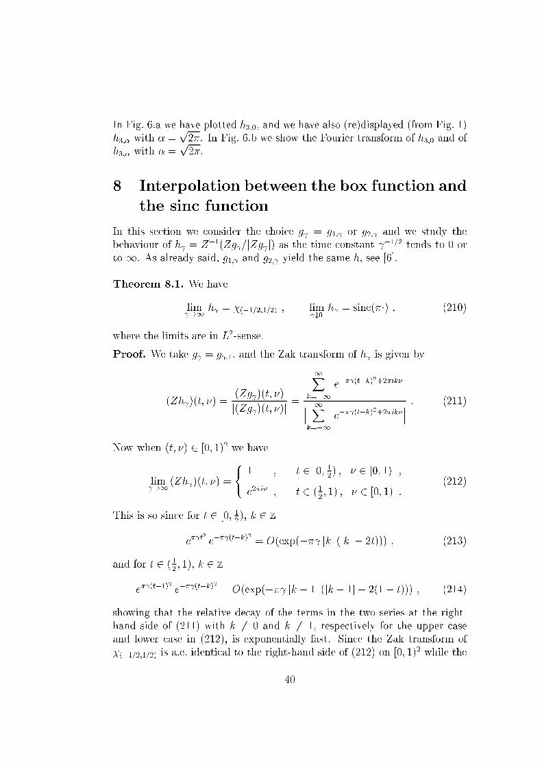
In Fig. 6.a we have plotted h3;0, and we have also (re)displayed (from Fig. 1)

h3;� with � =p2�. In Fig. 6.b we show the Fourier transform of h3;0 and of

h3;� with � =p2�.

8 Interpolation between the box function and

the sinc function

In this section we consider the choice g = g1; or g2; and we study the

behaviour of h = Z�1(Zg =jZg j) as the time constant �1=2 tends to 0 or

to 1. As already said, g1; and g2; yield the same h, see [6].

Theorem 8.1. We have

lim !1

h = �(�1=2;1=2) ; lim #0

h = sinc(��) ; (210)

where the limits are in L2-sense.

Proof. We take g = g ;1, and the Zak transform of h is given by

(Zh )(t; �) =(Zg )(t; �)

j(Zg )(t; �)j=

1Xk=�1

e�� (t�k)2+2�ik�

��� 1Xk=�1

e�� (t�k)2+2�ik�

���: (211)

Now when (t; �) 2 [0; 1)2 we have

lim !1

(Zh )(t; �) =

8<:

1 ; t 2 [0; 12) ; � 2 [0; 1) ;

e2�i� ; t 2 (12; 1) ; � 2 [0; 1) :

(212)

This is so since for t 2 [0; 12), k 2 Z

e� t2

e�� (t�k)2

= O(exp(�� jkj (jkj � 2t))) ; (213)

and for t 2 (12; 1), k 2 Z

e� (t�1)2

e�� (t�k)2

= O(exp(�� jk � 1j (jk � 1j � 2(1� t))) ; (214)

showing that the relative decay of the terms in the two series at the right-hand side of (211) with k 6= 0 and k 6= 1, respectively for the upper case

and lower case in (212), is exponentially fast. Since the Zak transform of

�(�1=2;1=2) is a.e. identical to the right-hand side of (212) on [0; 1)2 while the

40

convergence in (212) is certainly in L2([0; 1)2)-sense, we easily get the �rst

issue in (210) with L2(R)-convergence.

Next we consider the second limit in (210). The Fourier transform of g equals g1= , whence, see the last paragraph in Sec. 1, the Fourier transform

of h equals h1= . Now since the two right-hand side functions in (210) are

Fourier pairs, the second limit relation in (210) follows from the �rst one.

This completes the proof.

In Fig. 7 we have displayed h for several values of (ranging from very

small to very large).

Note. As the proof of Theorem 8.1 shows, one has similar limit relations

as in (210) for a considerably wider class of windows g than Gaussians or

hyperbolic secants. Denoting g = 1=2 g( �) and h = Z�1(Zg =jZg j), the�rst limit relation in (210) holds when g( s)=g( t) ! 0 suÆciently rapidly

when s > t � 0 and ! 1. Similarly, the second limit relation in (210)holds when (Fg)( �)=(Fg)( �)! 0 suÆciently rapidly when � > � � 0 and !1. Evidently, the two-sided exponential does satisfy the �rst condition

but fails to satisfy the second one.

41

Acknowledgements

It is a great pleasure for the author to acknowledge Dr. Thomas Strohmer

for his constant interest and attentiveness while the research leading to this

paper was carried out. Dr. Strohmer's keen observations de�nitely reshaped

the process by which the results were obtained and presented. The author

also wants to thank him for help in producing the �gures.

42

References

[1] I. Daubechies, The wavelet transform, time-frequency localization and

signal analysis, IEEE Trans. Inform. Theory, vol. 36, pp. 961{1005, 1990.

[2] I. Daubechies, \Ten Lectures on Wavelets", Philadelphia: SIAM, 1992.

[3] H.G. Feichtinger and T. Strohmer, Eds., \Gabor Analysis and Algo-

rithms { Theory and Applications", Boston: Birkh�auser, 1998.

[4] K. Gr�ochenig, \Foundations of Time-Frequency Analysis", Boston:

Birkh�auser, 2000.

[5] A.J.E.M. Janssen, Zak transforms with few zeros and the tie, to appear

in \Advances in Gabor Analysis" (H.G. Feichtinger and T. Strohmer,Eds.).

[6] A.J.E.M. Janssen and T. Strohmer, Hyperbolic secants yield Gaborframes, submitted to Appl. Comp. Harmonic Anal.

[7] P.D. Einziger, Gabor expansion of an aperture �eld in exponential ele-mentary beams, IEE Electronics Letters 24, pp. 665{666, 1988.

[8] A.J.E.M. Janssen and T. Strohmer, Characterization and computation

of canonical tight windows for Gabor frames, to appear in J. Four. Anal.Appl.

[9] M. Abramowitz and I.A. Stegun, \Handbook of Mathematical Func-tions", New York: Dover, 1970 (9th printing).

[10] P.F. Byrd and M.D. Friedman, \Handbook of Elliptic Integrals for En-

gineers and Physicists", Berlin: Springer, 1971 (2nd edition).

[11] A.P. Prudnikov, Y.A. Brychkov and O.I. Marichev, \Integrals and Se-

ries, Vol. 1: Elementary Functions", New York: Gordon and Breach,1986.

[12] M.R. Spiegel, \Mathematical Handbook of Formulas and Tables"

(Schaum's outline series), New York: McGraw-Hill, 1968.

43

Figure captions

Fig. 1. Tight frame generating window h associated to g = g1; and g = g3;�of (9) and (10) according to (7) with = 1 and � =

p2�.

Fig. 2. Zak tight window h3;� and frame tight window ah3;� associated to

g3;� in (10) for � =p2� and a = b =

p0:9.

Fig. 3. Zak tight window h3;� and frame tight window ah3;� associated to

g3;� in (10) for � =p2� and a = b =

p0:99.

Fig. 4. The points s0; :::; s6 2 [0; 1) as in (95) with p = 4, a = 49=60,

s0 = 1=24, together with the graphs of r2(s), r1(s) see (78), for

s 2 [0; 1].

Fig. 5. The canonical dual gd3;� formally associated to g3;� of (10) according

to (109) and explicitly given by (110), (111) for � =p2�.

Fig. 6. a. The limiting form of h3;� as � # 0 with g3;� as in (10), given inintegral form in (187), and h3;� with � =

p2�.

b. The Fourier transform of h3;� as � # 0 with g3;� as in (10), and

the Fourier transform of h3;� with � =p2�.

Fig. 7. The tight frame generating window h associated to g = g1; of (9)

for the values = 0:1; 0:5; 1; 2; 10.

44

−6 −4 −2 0 2 4 6

−0.4

−0.2

0

0.2

0.4

0.6

0.8

1

1.2h

3,αh

1,γ

Figure 1.

45

−6 −4 −2 0 2 4 6

−0.2

0

0.2

0.4

0.6

0.8

1 ab=1 ab=0.9

Figure 2.

46

−6 −4 −2 0 2 4 6

−0.2

0

0.2

0.4

0.6

0.8

1 ab=1 ab=0.99

Figure 3.

47

0 1s

1

2

3

4

5

6

0s0

a1-a

r2(s) r1(s)

s5 s4 s3 s2 s1 s6

Figure 4.

48

−5 −4 −3 −2 −1 0 1 2 3 4 5−3

−2

−1

0

1

2

3analyticZak

Figure 5.

49

−6 −4 −2 0 2 4 6−0.4

−0.2

0

0.2

0.4

0.6

0.8

1h3,0

h3,α, α=(2π)1/2

Figure 6a.

50

−6 −4 −2 0 2 4 6−0.4

−0.2

0

0.2

0.4

0.6

0.8

1 h 3,0

h 3,α, α=(2π)1/2

Figure 6b.

51

−6 −4 −2 0 2 4 6−0.4

−0.2

0

0.2

0.4

0.6

0.8

1γ=0.1γ=0.5γ=1 γ=2 γ=10

Figure 7.

52