arX

iv:1

411.

2603

v5 [

hep-

th]

21

Apr

201

8

On Functional Representations of the Conformal Algebra

Oliver J. Rosten

oliver.rosten@gmail.com

Abstract

Starting with conformally covariant correlation functions, a sequence of functional representa-

tions of the conformal algebra is constructed. A key step is the introduction of representations

which involve an auxiliary functional. It is observed that these functionals are not arbitrary but

rather must satisfy a pair of consistency equations corresponding to dilatation and special confor-

mal invariance. In a particular representation, the former corresponds to the canonical form of

the Exact Renormalization Group equation specialized to a fixed-point whereas the latter is new.

This provides a concrete understanding of how conformal invariance is realized as a property of

the Wilsonian effective action and the relationship to action-free formulations of conformal field

theory.

Subsequently, it is argued that the conformal Ward Identities serve to define a particular rep-

resentation of the energy-momentum tensor. Consistency of this construction implies Polchinski’s

conditions for improving the energy-momentum tensor of a conformal field theory such that it is

traceless. In the Wilsonian approach, the exactly marginal, redundant field which generates lines

of physically equivalent fixed-points is identified as the trace of the energy-momentum tensor.

In loving memory of Francis A. Dolan.

1

CONTENTS

I. Introduction 3

A. Conformal Field Theories 3

B. The Exact Renormalization Group 5

C. The Energy-Momentum Tensor 8

II. Conformal Symmetry in QFT 11

A. Elementary Properties of the Conformal Group 11

B. Correlation Functions 12

C. From Sources to the Fundamental Field 14

D. From The Fundamental Field to the ERG 17

III. Polchinski’s Equation from the Conformal Algebra 22

IV. The Energy-Momentum Tensor 27

A. Proposal 27

B. Justification 30

1. Existence 30

2. Conformal Covariance 34

3. Uniqueness 35

C. Conformal Invariance 37

D. Quasi-Local Representation 38

E. The Gaussian Fixed-Point 40

1. Para-Schwinger Functional Representation 41

2. ERG Representation 42

F. A Non-Unitary Example 43

V. Conclusions 45

Acknowledgments 47

References 48

2

I. INTRODUCTION

A. Conformal Field Theories

The essential information content of any quantum field theory (QFT) is encoded in its

correlation functions. As such, the various different approaches to the former ultimately

amount to different strategies for computing the latter. In an ideal situation, it could be

imagined that the correlation functions are determined entirely by some symmetry, allowing

one to concentrate solely on the representation theory of the appropriate algebra, having

dispensed with standard notions such as an action and corresponding path integral.

In general, such a strategy is not available. However, a partial realization occurs for QFTs

exhibiting conformal symmetry—the Conformal Field Theories (CFTs). If we suppose that

the correlation functions involve a set of local objects, {O(x)}, then a special set of ‘con-

formal primary fields’, Oi(x), can be identified for which the correlation functions exhibit

covariance under global conformal transformations. Focussing on the conformal primaries,

the various two and three-point correlation functions are determined by the conformal sym-

metry in terms of the a priori unknown CFT data: the scaling dimensions, ∆i, spins and

three-point coefficients, Cijk. At the four-point level and beyond, the direct constraints of

conformal symmetry are weaker, still.

Further progress can be achieved by applying the Operator Product Expansion (OPE).

Within correlation functions, consider taking a limit such that the positions of two of the

fields approach each other. According to the OPE, in this limit the pair of fields can be

replaced by a linear sum over fields; schematically, this can be written

Oa(x)Ob(y) ∼∑

c

f cab(x− y)Oc(y). (1.1)

A particularly powerful effect of conformal symmetry is that the complete content of the

OPE can be rephrased in terms of just the conformal primary fields. If the OPE converges

for finite separations, then n-point correlation functions can be determined in terms of n−1

point correlation functions. In this manner, the content of conformal field theories can, in

principle, be boiled down to the CFT data introduced above.

However, to determine the various combinations of CFT data which correspond to ac-

tual CFTs (possibly subject to constraints, such as unitarity) requires further input. One

approach is to exploit associativity of the OPE to attempt to constrain the CFT data (this

3

technique is known as the conformal bootstrap). In general, the task is extremely challeng-

ing since one can expect an infinite number of conformal primaries, the scaling dimensions

of which must be self-consistently determined. Nevertheless, substantially inspired by work

of Dolan and Osborn [1–3], remarkable recent progress has been made in this area [4–10].

In two dimensions, additional structure is present. Whilst the global conformal group

is always finite dimensional, in d = 2 there exists an infinite dimensional local conformal

algebra, the Virasoro algebra. Fields can now be classified according to their transforma-

tions under local (rather than just global) conformal transformations and, as such, arrange

themselves into multiplets comprising a Virasoro primary and its descendants. In the sem-

inal paper [11] it was shown that there are a set of special theories, the ‘minimal models’

for which there are only a finite number of Virasoro primaries possessing known scaling

dimensions. This simplification is sufficient for the bootstrap procedure to determine the

CFT data and for all correlation functions to be expressible as solutions to linear partial

differential equations.

However, even in this situation, there are some natural questions to pose, at least coming

from the perspective of the path integral approach to QFT: is it possible to encode the

dynamics of these theories in an action and, if so, is there a concrete recipe for doing so? Is

this procedure possible for all such theories or only some of them? Are the resulting actions

guaranteed to be local and, if so, why? In this paper, it will be attempted to provide answers

to some of these questions and hopefully to offer a fresh perspective on others.

These questions are equally valid (and perhaps less academic) in situations where the

conformal bootstrap is insufficient to provide a complete understanding of the theories to

which it is applied. We will take the point of view that, in this situation, one approach is

to try to introduce an action formulation of the theory in question. Notice that this has

been deliberately phrased so as to reverse the logical order compared to the path integral

approach. Typically, within the path integral paradigm, the first thing that one does is write

down a (bare) action. The conformality or otherwise of the resulting theory must then be

determined. In our approach, however, we envisage starting with correlation functions which

are conformally covariant by assumption and then introducing the action as an auxiliary

construction.

At heart, the underlying philosophy of this paper is to take an intrinsically quantum

field theoretic starting point i.e. the symmetry properties of the correlation functions of

4

the theory at hand. The idea then is to show that, perhaps given certain restrictions,

this implies that (should one so desire) a local action can be constructed, from which the

correlation functions can, in principle, be computed. If one is to take QFT as fundamental,

this seems more philosophically satisfactory than taking a classical action as the starting

point. Moreover, it clarifies the relationship between two largely disassociated textbook

approaches to QFT.

B. The Exact Renormalization Group

As will be exposed in this paper, the formalism which binds together the classic CFT

approach to field theory with its path integral counterpart is Wilson’s Exact Renormalization

Group (ERG) [12]. Starting from conformally covariant correlation functions, the strategy

is to encode the information thus contained in various functional representations.1 Each

representation will yield different expressions both for the conformal generators and for

the conformal primaries and their descendants. The most direct representation follows from

introducing sources and embedding the correlation functions in the Schwinger functional,W(the subtleties of doing this in the presence of infrared (IR) and ultraviolet (UV) divergences

are discussed later). Associated with the Schwinger functional is a representation of the

conformal algebra; for CFTs, each of the generators annihilates W.

For simplicity, we will largely consider theories for which all conformal primary fields are

scalar (relaxing this, at least in the absence of gauge symmetry, is straightforward). More

importantly, we assume that there is at least one conformal primary field for which the

Schwinger functional—written in terms of the conjugate source, J—exists. To proceed, we

shift this source by the derivative of a new, auxiliary field:

J → J + ∂2ϕ, (1.2)

resulting in another representation of the conformal algebra. Note that ϕ will essentially

end up playing the role of the fundamental field (for brevity, we implicitly consider theories

which involve just a single fundamental field).

The form of the shift (1.2) may seem a little odd. Ultimately, it can be traced back to

1 While the correlation functions themselves are conformally covariant, we refer to the functionals as rep-

resenting a conformally invariant theory.

5

Morris’ observation that the Wilsonian effective action naturally generates the correlation

functions with an extra factor of momentum squared on each leg [13].

Next, we introduce a deformation of the Schwinger functional obtained by adding an

apparently arbitrary functional of ϕ and J which, amongst other things, means that the

deformed functional may depend separately on the field and the source. The motivation

for this follows from previous studies of the ERG: this deformed functional is recognized as

something which can be generated from a Wilsonian effective action, S. To put it another

way, we know the answer that we’re looking for!

Recall that, in the Schwinger functional representation, a CFT is such that the generators

annihilate W. This is translated into the statement that the generators in the new repre-

sentation annihilate exp−S. However, whereas the generators in the Schwinger functional

representation are linear in functional derivatives, in the new representation the generators

associated with dilatations and special conformal transformations are quadratic. The up-

shot of this is that two of the linear conditions implied by the annihilation of exp−S can be

replaced two by non-linear conditions on S. The first of these is identified with the fixed-

point version of an ERG equation and the second—constituting one of the central results of

this paper—is recognized as a new analogue of the special conformal consistency condition

discovered long ago by Schafer [14]. Associated with these conditions is a representation of

the conformal algebra in which the generators depend explicitly on the Wilsonian effective

action.

The non-linearity of the ERG equation seems to be crucial (as emphasised by Weg-

ner [15]). In the linear Schwinger functional representation, the scaling dimensions of the

fields must be determined in a self-consistent fashion using the bootstrap equations. In the

Wilsonian approach, a different strategy is used. One field2, with a priori unknown scaling

dimension, δ, is separated from the rest and used to formulate an ERG equation (as antic-

ipated above, we identify this field as the fundamental field). As such, it appears that an

ERG equation contains two unknowns: the Wilsonian effective action and δ. The correct

interpretation is that an ERG equation is a non-linear eigenvalue equation [16]; however,

this hinges on one further ingredient: we demand that the solutions to the ERG equation

are quasi-local.3

2 In much of the ERG literature, ‘operator’ is used in place of field; however, following CFT conventions,

we shall generally use the latter.3 By quasi-local it is meant that contributions to the action exhibit an expansion in positive powers of

6

It is the combination of non-linearity and quasi-locality which allows, in principle, for the

spectrum of δ to be extracted from the ERG equation. Indeed, by demanding quasi-locality,

the spectrum of possible values of δ can be shown to be discrete [17]. Let us emphasise that

the spectrum of δ does not correspond to the spectrum of fields within a given CFT; rather,

each value of δ obtained by solving the ERG equation corresponds to a different CFT.

Presuming that some solution to the ERG equation has been obtained, the second step

would be to compute the spectrum of fields. With both S and δ now known, the dilatation

generator has a concrete form. It now provides a linear eigenvalue equation for the fields

and their scaling dimensions. In general, the spectrum is rendered discrete by the condition

of quasi-locality: this is illustrated for the Gaussian fixed-point in [15, 17]. Within the

derivative expansion approximation scheme, see [16] for an excellent description of how

discreteness of the spectrum arises for non-trivial fixed-points.

From the perspective of different representations of the conformal algebra, it is locality,

together with non-linearity, which singles out the ERG representation as special. Remember

that the reason for considering elaborate representations of the conformal algebra is more

than just academic: part of the motivation is to provide tools for understanding conformal

field theories for which the conformal bootstrap seems intractable. In the ERG approach,

scale-invariant theories can be picked out from an equation by applying a constraint which

is easy to implement on the solutions: that of quasi-locality. The price one pays for this

is the introduction of a considerable amount of unphysical scaffolding, notably the UV

regularization. One can imagine other representations of the conformal algebra which entail

similar complication but without the redeeming feature of a simple condition which can be

imposed on solutions of the scale/special conformal consistency conditions.

An interesting question to ask is whether the set of conformal field theories (perhaps sub-

ject to constraints of physicality) is in one-to-one correspondence with the set of equivalence

classes of quasi-local actions. It is tempting and perhaps not too radical to speculate that,

at the very least for the sorts of theories which form the focus of this paper—non-gauge

theories, on a flat, static background, for which the energy-momentum tensor exists and is

non-zero—the answer is yes. While there are some suggestive numerical results [18], it is

desirable to have a proof, one way or the other. The thrust of this paper gives some clues as

derivatives. Equivalently, in momentum space, vertices have an all-orders expansion in powers of momenta.

Loosely speaking, at long distances a quasi-local action has the property that it reduces to a strictly local

form. Quasi-locality is discussed, at length, in [17].

7

to how this can be achieved (as discussed further in the conclusion) but at a rigorous level

the question remains unanswered, for now.

C. The Energy-Momentum Tensor

It is worth emphasising that the approach advocated above is precisely the opposite of

the standard path integral approach: our starting point is the correlation functions; then

we introduce sources; next we introduce a field and arrive at an action! Everything within

this picture, with the exception of the correlation functions, themselves, is an auxiliary

construction. As such, this sits rather uncomfortably with standard expositions of the role

of the energy-momentum tensor in QFT: for these tend to start with the classical action.

This tension is reconciled as follows. One of the key results of this paper is that, for

conformal field theories, the usual Ward identities associated with the energy-momentum

tensor should, in fact, be recognized as defining the energy-momentum tensor in a partic-

ular representation of the conformal algebra.4 To see how this comes about, consider the

Ward identity associated with translation invariance. Taking Tαβ to denote a quasi-local

representation of the energy-momentum tensor, we have [19]:

∂α⟨

Tαβ(x)O(δ)loc(x1) · · ·O

(δ)loc(xn)

⟩

= −n

∑

i=1

δ(d)(x− xi)∂

∂xiβ

⟨

O(δ)loc(x1) · · ·O

(δ)loc(xn)

⟩

(1.3)

where O(δ)loc is a quasi-local representation of the conformal primary field conjugate to J .

Multiplying by one source for each instance of the quasi-primary field and integrating over

the corresponding coordinates yields:

∂α⟨

Tαβ(x)J · O (δ)loc · · ·J · O

(δ)loc

⟩

= −J(x)∂βδ

δJ(x)

⟨

J ·O (δ)loc · · ·J ·O

(δ)loc

⟩

(1.4)

where, in accord with the notation of [20] (which we largely follow throughout this paper)

J · O ≡∫

ddx J(x)O(x).

Next, we sum over n and observe that the result can be cast in the form

∂αT (Sch)αβ = −J ∂β

δW[J ]

δJ, (1.5)

4 Actually, there are CFTs, such as the Mean Field Theories, for which the energy-momentum tensor does

not exist; this will be discussed further in section IVA.

8

where we have chosen to define T (Sch)αβ such that it is only contains connected contribu-

tions (multiplying by eW [J ] restores the disconnected pieces). A crucial point is that (mod-

ulo some subtleties to be dealt with later) we interpret T (Sch)αβ as a representation of the

energy-momentum tensor; the ‘Sch’ serves to reminds us that this representation involves

the Schwinger functional. When working in an arbitrary representation, we will utilize the

symbol Tαβ .Evidence will be assembled for this in section IV as follows. As we will see in section IVA,

the Schwinger functional representation makes it particularly transparent that the two main

ingredients on the right-hand side of (1.5), J and δW/δJ are (again, modulo some subtleties

to be discussed later) representations of a pair of conformal primary fields with scaling

dimensions, d− δ and δ:

O(d−δ)J (x) = J(x), (1.6)

O(δ)J (x) =

δW[J ]

δJ(x). (1.7)

The subscript J adorning the conformal primary fields is a reminder that we are considering

a particular representation. Let us emphasise again that this particular representation of

O (δ) is non-local and that we will see later how to obtain a reassuringly local representation,

via the ERG.

Existence of Tαβ is established in section IVB1. The basic idea is to exploit the fact

that O(d−δ)J and O

(δ)J can be combined in various ways to express translation, rotation and

dilatation invariance. For example, translational invariance of the Schwinger functional can

be stated as

∂βJ ·δW[J ]

δJ= 0,

which suggests the existence of a tensor field such that

O(d−δ)J (x)∂βO

(δ)J (x) = −∂αFαβ(x).

(As will be discussed more fully later, this is not quite the full story: existence of a quasi-

local representation of the theory is required.) Rotational invariance implies symmetry of

Fαβ . Furthermore, it will be shown, under certain conditions, that Fαβ can be ‘improved’

in such a way that its trace corresponds to the Ward identity associated with dilatation

invariance. Assuming this improvement to be done, conformal invariance is confirmed in

section IVC.

9

This analysis of the improvement procedure will be seen to have close parallels to that of

Polchinski’s classic paper [21]. Indeed, as in the latter, a sufficient condition for this improve-

ment is essentially that primary vector fields of scaling dimension d− 1 are absent from the

spectrum. In the same paper, Polchinski completed an argument due to Zamolodchikov [22]

showing that, in two dimensions, the energy-momentum tensor of a scale-invariant theory

can be rendered traceless if the theory is unitary and the spectrum of fields is discrete. The

veracity of this for d > 2 has been much debated [23].

As additional confirmation of the consistency of our approach it will be shown in sec-

tion IVB2 that Tαβ has the same properties under conformal transformations as a tensor,

conformal primary field of scaling dimension, d. (We use the term field with care since the

associated representation is non-local, but henceforth will be less assiduous.) Let us empha-

sise that we are not claiming⟨

Tαβ⟩

is a representation of the energy-momentum tensor in the

sense of having the correct transformation properties under the appropriate representation

of the conformal group; only for the full Tαβ does this hold.

While this section began with the standard representation of the energy-momentum

tensor—i.e. a quasi-local object—from the perspective of this paper we view as more prim-

itive the non-local representation furnished by the Schwinger functional, Tαβ. For theories

supporting a quasi-local representation, Tαβ can be recovered via the ERG, as will become

apparent in section IVD. With this achieved, another of the central results of this paper

will become apparent: in the ERG representation, the trace of the energy-momentum tensor

is nothing but the exactly marginal, redundant field possessed by every critical fixed-point.

(Redundant fields correspond to quasi-local field redefinitions.) It is the existence of this

field which causes quasi-local fixed-point theories to divide up into equivalence classes: every

fixed-point theory exists as a one-parameter family of physically equivalent theories [15–

17, 24, 25]. This is the origin of the quantization of the spectrum of δ.

The construction of the energy-momentum tensor will be illustrated in section IVE using

the example of the Gaussian fixed-point; section IVF demonstrates how the construction

breaks down for a simple, non-unitary theory.

10

II. CONFORMAL SYMMETRY IN QFT

A. Elementary Properties of the Conformal Group

In this section, we recall some basic features of the conformal group; henceforth, unless

stated otherwise, we work in Euclidean space. The generators {Pµ,Mµν ,D,Kµ} respectivelygenerate translations, rotations, dilatations (scale transformations) and special conformal

transformations; the non-zero commutators are:

[

D,Pµ

]

= Pµ,[

Mµν ,Mσρ

]

= δµσMνρ − δνσMµρ − δµρMνσ + δνρMµσ,[

Mµν ,Pσ

]

= δµσPν − δνσPµ,[

Mµν ,Kσ

]

= δµσKν − δνσKµ,[

D,Kµ

]

= −Kµ,[

Kµ,Pν

]

= 2δµνD + 2Mµν . (2.1)

Though it will not exploited in this paper, it is worth noting that the commutation relations

can be recast in a manner which makes explicit the isomorphism between the conformal

group and SO(d+ 1, 1) (see, for example, [19]).

A scalar conformal primary field, O(x), with scaling dimension ∆, satisfies5

PµO = ∂µO , MµνO = LµνO , DO = D(∆)O , KµO = K(∆)

µO , (2.2)

where {∂µ, Lµν , D(∆), K(∆)

µ} are taken such that they satisfy a version of the commutation

relations above in which the signs are flipped. This is crucial if (2.2) is to be consistent with

the commutation relations. For example, it follows from (2.2) that

[

D,Kµ

]

O(x) =[

K(∆)µ, D

(∆)]

O(x), (2.3)

from which we deduce that[

D(∆), K(∆)µ

]

= +K(∆)µ, as compared with

[

D,Kµ

]

= −Kµ

in (2.1). With this in mind, we take:

LµνO(x) =(

xµ∂ν − xν∂µ)

O(x), (2.4a)

D(∆)O(x) =

(

x · ∂ +∆)

O(x), (2.4b)

K(∆)µO(x) =

(

2xµ(

x · ∂ +∆)

− x2∂µ)

O(x). (2.4c)

5 Were we to work in an operator formalism, the expressions on the left-hand sides would appear as com-

mutators.

11

The general modification of (2.2) appropriate to non-scalar fields can be found in [19]. For

our purposes, we explicitly give the version appropriate to tensor fields:

MµνOα1...αn(x) = LµνOα1...αn

(x) +n

∑

i=1

(

δµαiδγν − δναi

δγµ)

Oα1...γ...αn(x), (2.5a)

KµOα1...αn(x) = K(∆)

µOα1...αn(x) + 2

n∑

i=1

(

δµαiδγβ − δβαi

δγµ)

xβOα1...γ...αn(x). (2.5b)

These relationships will play an important role when we deal with the energy-momentum

tensor in section IV.

Let us emphasise that, at this stage, the representation of the {Pµ,Mµν ,D,Kµ} and

the O(x) are yet to be fixed; a key theme of this paper will be the exploration of certain

representations thereof, some of which are non-standard.

B. Correlation Functions

In the context of QFT, the chief consequence of conformal symmetry is that various corre-

lation functions are annihilated by {∂µ, Lµν , D(∆), K(∆)

µ}. Specifically, correlation functions

involving only the conformal primaries are annihilated by all members of the set, whereas

those involving descendant fields (the derivatives of the conformal primaries) are annihilated

only by those corresponding to translations, rotations and dilatations. Thus we have, for all

n,( n∑

j=1

K(∆ij)µ(xj)

)

⟨

Oi1(x1) · · ·Oin(xn)⟩

= 0, ∀ i1, . . . , in (2.6)

whereas the remaining conditions read6 , now for all a1, . . . , an:

( n∑

j=1

∂

∂xjµ

)

⟨

Oa1(x1) · · ·Oan(xn)⟩

= 0,

( n∑

j=1

Lµν(xj)

)

⟨

Oa1(x1) · · ·Oan(xn)⟩

= 0,

( n∑

j=1

D(∆ij)(x)

)

⟨

Oa1(x1) · · ·Oan(xn)⟩

= 0.

(2.7)

The ultimate aim is to find solutions to (2.6) and (2.7) that correspond to acceptable QFTs.

6 Indices near the beginning of the alphabet are understood to label all fields, rather than just the conformal

primaries.

12

A key step for what follows is to introduce a set of sources, Ji(x), conjugate to the

conformal primary fields Oi(x) (any Euclidean indices are suppressed). There is no need

to introduce sources for the descendants since the associated correlation functions can be

generated from the analogue involving just primaries by acting with appropriate derivatives.

Restricting to conformal primary fields, we tentatively rewrite (2.6) and (2.7) as(

∑

i

K(d−∆i)µ Ji ·

δ

δJi

)

eW [{J}] = 0, (2.8a)

(

∑

i

D(d−∆i)Ji ·δ

δJi

)

eW [{J}] = 0, (2.8b)

(

∑

i

∂µJi ·δ

δJi

)

eW [{J}] = 0, (2.8c)

(

∑

i

LµνJi ·δ

δJi

)

eW [{J}] = 0, (2.8d)

where

eW [{J}] =⟨

e∑

i Ji·Oi⟩

(2.9)

In general, considerable care must be taken defining the expectation value of exponen-

tials, due to both IR and UV singularities. However, this paper will only directly utilize

expectation values involving J (which, we recall, can loosely be thought of as coupling to

the lowest dimension conformal primary field); indeed, for brevity we will henceforth deal

only with this single source, the scaling dimension of which is d− δ (it is a simple matter to

insert the remaining sources, should one so desire).

At certain stages, we will simply assume that the Schwinger functional involving solely J ,

W[J ], is well defined. To be precise, when we talk of existence of the Schwinger functional, it

is meant that the correlation functions of the field conjugate to J can be directly subsumed

into W[J ] and so the naıve identities (2.8a)–(2.8d) hold. Note that existence of W[J ] is

considered a separate property from W[J ] being non-zero.

By definition, we take Ji · Oi to have zero scaling dimension; this implies that Ji(x) has

scaling dimension d −∆i. This leads us to the first of several functional representations of

the conformal generators that will be presented in this paper.

Representation 1 Schwinger Functional Representation

Pµ = ∂µJ ·δ

δJ, Mµν = LµνJ ·

δ

δJ, (2.10a)

D = D(d−δ)J · δδJ, Kµ = K(d−δ)

µJ ·δ

δJ. (2.10b)

13

It is easy to check that these generators satisfy the conformal algebra by utilizing (2.4a),

(2.4b) and (2.4c), together with the following relationships which follow from integrating by

parts:

∂µJ ·δ

δJ= −J · ∂µ

δ

δJ, LµνJ ·

δ

δJ= −J · Lµν

δ

δJ, (2.11a)

D(d−δ)J · δδJ

= −J ·D(δ) δ

δJ, K(d−δ)

µJ ·δ

δJ= −J ·K(δ)

µδ

δJ. (2.11b)

Note that the fact that {∂µ, Lµν , D(∆), K(∆)

µ} satisfy a version of the conformal commutation

relations in which the order of the commutators is flipped is crucial.

Now that we have a concrete functional representation of the conformal algebra, it is ap-

propriate to mention a subtlety pertaining to volume terms. To illustrate this issue, consider

the effect of the dilatation operator on an integrated field. Recalling (2.2) and (2.4b), it is

apparent that we expect

D∫

ddxO(x) = (∆− d)∫

ddxO(x). (2.12)

In deriving this, we have implicitly assumed that O depends on a field which dies of suffi-

ciently rapidly at infinity. However, for the identity operator this is not the case. To match

the two sides of (2.12) in this situation—and bearing in mind that ∆ = 0—suggests that

the dilatation generator should be supplemented by a term

−dV ∂

∂V,

with V being the volume of the space on which the field theory lives. For this paper,

however, we will generally ignore volume terms; as such, we henceforth understand equality

in functional equations to hold only up to volume terms. This issue will be addressed more

fully in [26].

C. From Sources to the Fundamental Field

Up until this point, our functional representation has utilized sources. The transition to

fields proceeds in several steps, along the way giving new representations of the conformal

algebra. The first such step is provided by the shift (1.2). Clearly, at this stage, the

dependence on J and ϕ will not be independent. However, the link will be severed in a

14

subsequent representation. To prepare for this severing, our aim in this section is, given

the shift (1.2), to construct a representation in which the generators involve functional

derivatives with respect to ϕ (rather than ∂2ϕ).

As mentioned earlier, we anticipate that ϕ will play the role of the fundamental field.

Before proceeding, it is worth pointing out that there is a subtlety over precisely what is

meant by the latter. Strictly speaking, both the Wilsonian effective action and the field to

which J couples are built out of ϕ. Within the ERG representation (and assuming sufficiently

good IR behaviour), ϕ coincides with a conformal primary field only up to non-universal

terms, which vanish in the limit that the regularization is removed. While this subtlety will

be largely glossed over since it seems to have no great significance, the issue of theories for

which bad IR behaviour prevents ϕ from corresponding to a conformal primary in any sense

will be returned to, later.

With the aim of producing a representation of the generators involving functional deriva-

tives with respect to ϕ, we exploit the commutators[

∂2, D(∆)]

= 2∂2,[

∂2, K(∆)µ

]

= 4(∆− δ0)∂µ + 4xµ∂2,

(2.13)

where δ0 (which we recognize as the canonical dimension of the fundamental field) is given

by

δ0 ≡d− 2

2. (2.14)

Next, define G0 to be Green’s function for −∂2:

− ∂2G0(x) = δ(d)(x). (2.15)

Employing notation such that, for fields ϕ(x), ψ(x) and kernel K(x, y)

ϕ ·K · ψ ≡∫

ddx ddy ϕ(x)K(x, y)ψ(y), (2.16)

observe that

D(d−δ)J · δδJW[J ]

∣

∣

∣

∣

∣

J=∂2ϕ

= D(d−δ)(∂2ϕ) · δ

δ(∂2ϕ)W[∂2ϕ]

= −D(d−δ)(∂2ϕ) · G0 ·δ

δϕW[∂2ϕ]

=(

[

∂2, D(d−δ)]

ϕ− ∂2(

D(d−δ)ϕ))

· G0 ·δ

δϕW[∂2ϕ]

= D(d−δ−2)ϕ · δδϕW[∂2ϕ], (2.17)

15

where we recall from the introduction that δ is the scaling dimension of the fundamental

field. Performing similar manipulations for the special conformal generator we arrive at:

D(d−δ)J · δδJW[J ]

∣

∣

∣

∣

∣

J=∂2ϕ

= D(δ−η)ϕ · δδϕW[∂2ϕ], (2.18a)

K(d−δ)µJ ·

δ

δJW[J ]

∣

∣

∣

∣

∣

J=∂2ϕ

= K(δ−η)µϕ ·

δ

δϕW[∂2ϕ]− 2η ∂µϕ · G0 ·

δ

δϕW[∂2ϕ], (2.18b)

where we have introduced the anomalous dimension, η, defined via

δ = δ0 + η/2. (2.19)

Representation 2 Para-Schwinger Functional Representation

Pµ = Pµ ≡ ∂µJ ·δ

δJ+ ∂µϕ ·

δ

δϕ, (2.20a)

Mµν = Mµν ≡ LµνJ ·δ

δJ+ Lµνϕ ·

δ

δϕ, (2.20b)

D = D ≡ D(d−δ)J · δδJ

+D(δ−η)ϕ · δδϕ, (2.20c)

Kµ = Kµ ≡ K(d−δ)µJ ·

δ

δJ+K(δ−η)

µϕ ·δ

δϕ− 2η ∂µϕ · G0 ·

δ

δϕ, (2.20d)

where Pµ, Mµν , . . . correspond to the expressions for the various generators in the present

representation. It is straightforward to confirm from (2.4a), (2.4b) and (2.4c), together

with translational and rotational invariance of G0, that these generators satisfy the requisite

commutation relations. In this representation, a conformal field theory is such that each of

these generators annihilates W[J + ∂2ϕ].

Before introducing the next representation, it is worth mentioning that the functional

W[J + ∂2ϕ] may have different (quasi)-locality properties with respect to J and ϕ. For

non-trivial fixed-points this will not be the case, as can be seen at the two-point level. In

momentum space, the two-point correlation function goes like 1/p2(1−η/2). For non-trivial

fixed-points, η/2 is some non-integer number. While multiplying by a factor of p2 removes the

divergence as p2 → 0, it does not remove the non-locality. For trivial fixed-points, however,

non-locality may be ameliorated. This can be convenient and is exploited in section IVE.

16

D. From The Fundamental Field to the ERG

The aim now is to go from this representation to one in which the dynamics of the theory

is encoded in some auxiliary object. To begin, we introduce an auxiliary functional, U ,which, save for insisting translational and rotational invariance, we leave arbitrary for now.

From here, we define:

WU [ϕ, J ] ≡ −W[J + ∂2ϕ] + U [ϕ, J ]. (2.21)

Notice that WU [ϕ, J ] may depend independently on J and ϕ. The arbitrariness in U is a

manifestation of the freedom inherent in constructing ERGs, which has been recognized since

the birth of the subject [15, 24]. As particularly emphasised in [27], this can be understood

from deriving the ERG equation via a quasi-local field redefinition under the path integral,

which will be elaborated upon at the end of this section. In section III we will focus on a

particular choice of U which turns out to reproduce what is essentially Polchinski’s ERG

equation.

The idea now is to encode the dynamics in an object, S[ϕ, J ], and introduce an operator,

Y (about which more will be said, below), such that

eYe−S[ϕ,J ] = e−WU [ϕ,J ]. (2.22)

Thus, given S we can, in principle, recover the correlation functions. In this sense, S encodes

the dynamics of the theory. It should be pointed out that any vacuum contributions to the

Wilsonian effective action are unconstrained within our approach. The conditions on WU

implied by conformal invariance are blind to vacuum terms. Consequently, we are free to

add any vacuum term we like to U which amounts, via (2.22), to an arbitrary vacuum

contribution to the Wilsonian effective action.

Before moving on let us not that, in general, the Wilsonian approach deals not just

with scale (or conformally) invariant theories but with theories exhibiting scale dependence.

Scale-independent actions are typically denoted by S⋆ and solve the fixed-point version of

an ERG equation. However, since this paper will only ever deal with fixed-point quantities,

the ⋆ will henceforth be dropped.

There is an implicit assumption that it is possible to find a non-trivial Y such that (2.22)

exists. Given this, a representation can be constructed as follows. Given a generator, g, and

17

a representation of this generator, denoted by G , define

GU ≡ e−Ye−U−→G eUeY , (2.23)

where the arrow indicates that the generator acts on everything to their right, with it

being understood that further terms may follow the eY (without the arrow, we would take

the generator just to act on the explicitly written terms to its right). By construction, if

generators G and G ′ satisfy some commutation relation, then the same is true of GU and

G ′U . Immediately, this allows us to construct a representation as follows.

Representation 3 Auxiliary functional representation

Pµ = PUµ, (2.24a)

Mµν = MUµν , (2.24b)

D = DU , (2.24c)

Kµ = KUµ. (2.24d)

For a conformal field theory, in this representation, each generator annihilates e−S[ϕ,J ], as

follows from (2.21), (2.22) and (2.23).

Let us now explore some possibilities for Y . Translation invariance of the correlation

functions and of U implies that(

∂µJ ·δ

δJ+ ∂µϕ ·

δ

δϕ

)

e−WU [ϕ,J ] = 0, (2.25)

with a similar expression implied by rotational invariance. Next consider substituting for

WU using (2.22) and commuting eY to the left-hand side. Now demand manifest translation

invariance of S, by which we mean7

(

∂µJ ·δ

δJ+ ∂µϕ ·

δ

δϕ

)

e−S[ϕ,J ] = 0. (2.26)

This, together with the similar constraint coming from demanding manifest rotational in-

variance, implies[

eY , ∂µϕ ·δ

δϕ

]

eS[ϕ,J ] = 0,

[

eY , Lµνϕ ·δ

δϕ

]

eS[ϕ,J ] = 0. (2.27)

7 It is tempting to speculate that relaxing this requirement may be illuminating in the context of lattice

theories.

18

The most obvious solution to these constraints is Y = bϕ · δ/δϕ, for some constant b.

However, in this case S[ϕ] is related to WU by rescaling each leg of every vertex of the

latter by a factor of e−b, which gives us nothing new. Instead, we solve the constraints by

introducing a kernel, G(

(x− y)2)

, and taking

Y =1

2

δ

δϕ· G · δ

δϕ. (2.28)

Typically, G has, roughly speaking, the form of a regularized propagator (care must be

taken with this identification, as discussed in [17]). Given a momentum space UV cutoff

function, K(p2), and using the same symbol for position-space space objects and their Fourier

transforms, we write the Fourier transform of G as

G(p2) = K(p2)

p2. (2.29)

Of course, we have been guided to (2.28) and (2.29) by our pre-existing knowledge of both

the form of the ERG equation and the (related) role of the propagator in the standard

path integral approach to QFT. Let us stress that we have not derived these equations

and the uniqueness or otherwise of this particular solution is an important question to

answer, but beyond the scope of this paper. Given our prior knowledge of what to look for,

we anticipate that (2.28) and (2.29) will lead to a useful representation of the conformal

algebra (as discussed in the introduction, by ‘useful’ we mean that the constraint which

picks out physically acceptable theories is easy to implement; for the ERG this constraint

is quasi-locality). Before moving on, let us mention that (2.29) suffers from IR problems in

d = 2.8 Strictly speaking, this suggests that in d = 2 we should work in finite volume, at

least at intermediate stages.

Observe that it is possible to simplify the expressions for Pµ and Mµν . Since U is taken

to be invariant under translations and rotations, we can write

PUµ = e−Y−→Pµe

Y , MUµν = e−Y−→M µνe

Y . (2.30)

Given (2.27), it is tempting to try to simplify these expressions further, but a little care

must be taken. If these generators act on something which is transitionally and rotationally

invariant, then Pµ andMµν are transparent to eY which can be trivially commuted to the

8 Indeed the true propagator at the Gaussian fixed-point in d = 2 has logarithmic behaviour, emphasising

that the interpretation of G as a regularized propagator must be taken with a pinch of salt.

19

left, whereupon it is annihilated by e−Y , leaving behind just Pµ. But suppose, for example,

that Pµ acts on something not translationally invariant, such as

Aµ[ϕ] ≡1

2

∫

ddx

∫

ddy ϕ(x)ϕ(y)(x+ y)µF(

(x− y)2)

.

Using (2.28), it is easy to check that

[

Y , ∂µϕ ·δ

δϕ

]

Aν [ϕ] = δµνtrG · F.

The origin of this remainder relates to the discussion under (2.12); indeed, for many purposes

of interest it is consistent to take PUµ = Pµ.

Finally, we construct a representation in which the generators of dilatations and special

conformal transformations contain the action. Recalling (2.23), let us define

GS ≡ eS−→G Ue

−S . (2.31)

By construction it is apparent that, if GU and G ′U satisfy some commutation relation, then

so too do GS and G ′S , leading to the next representation.

Representation 4 ERG representation

Pµ = PSµ, (2.32a)

Mµν = MSµν , (2.32b)

D = DS , (2.32c)

Kµ = KSµ. (2.32d)

We will now study some of the properties of the last two representations. As remarked

above, in the auxiliary functional representation, a conformal field theory is such that e−S

is annihilated by each of the generators. For translations and rotations, this implies that S,itself, is thus annihilated. However, the same is not true for dilatations and special conformal

transformations. In the ERG representation, the associated constraints are most naturally

expressed as

ES [ϕ, J ] = eS[ϕ,J ]DUe−S[ϕ,J ] = 0, (2.33a)

ESµ[ϕ, J ] = eS[ϕ,J ]KUµe−S[ϕ,J ] = 0. (2.33b)

20

These translate into non-linear constraints on S, as we will see in an explicit example in the

next section.

Indeed, Given certain restrictions (pertaining to quasi-locality) to be discussed in sec-

tion III, (2.33a) will be recognized as nothing but an ERG equation (in the presence of

sources) specialized to a fixed-point. Equation (2.33b) is an additional constraint on the

action enforcing conformal invariance, along the lines of [14]. If we choose to restrict U to

depend only on ϕ, then the only source dependence in (2.33a) occurs through the action and

the Oi can be picked out of the latter in a simple manner. Anticipating this, let us reinstate

all sources and write

S[ϕ, {J}] = S[ϕ]−∑

i

Ji ·Oi + . . . (2.34)

Substituting into (2.33a) and (2.33b), it is apparent that

DS [ϕ]Oi(x) = D(∆i)Oi(x), (2.35a)

KSµ[ϕ]Oi(x) = K(∆i)µOi(x), (2.35b)

where DS [ϕ] and KSµ[ϕ] correspond to the pieces of DS and KSµ which remain when the

source is set to zero. This pair of equations confirms our expectation that the sources are

conjugate to the fields, as expected. Note that the constraint of quasi-locality is necessary

for the promotion of these equations to eigenvalue equations for the scaling dimensions, ∆i,

as mentioned in section IB.

Let us conclude this section by discussing in a little more detail how the freedom inherent

in U is related to the freedom inherent in the ERG. For (2.33a) to correspond to a bona-fide

ERG equation, DU must on the one hand be quasi-local and, on the other, must be such

that (up to vacuum terms), (2.33a) can be cast in the form [27]

δ

δϕ·(

Ψe−Stot[ϕ,J ])

= 0, (2.36)

where

Stot[ϕ] ≡ 1

2ϕ · G−1 · ϕ+ S[ϕ] (2.37)

and Ψ (which itself depends on the action) is quasi-local. It will be apparent from the next

section that the constraint of quasi-locality rules out the apparently simplest choice U = 0.

21

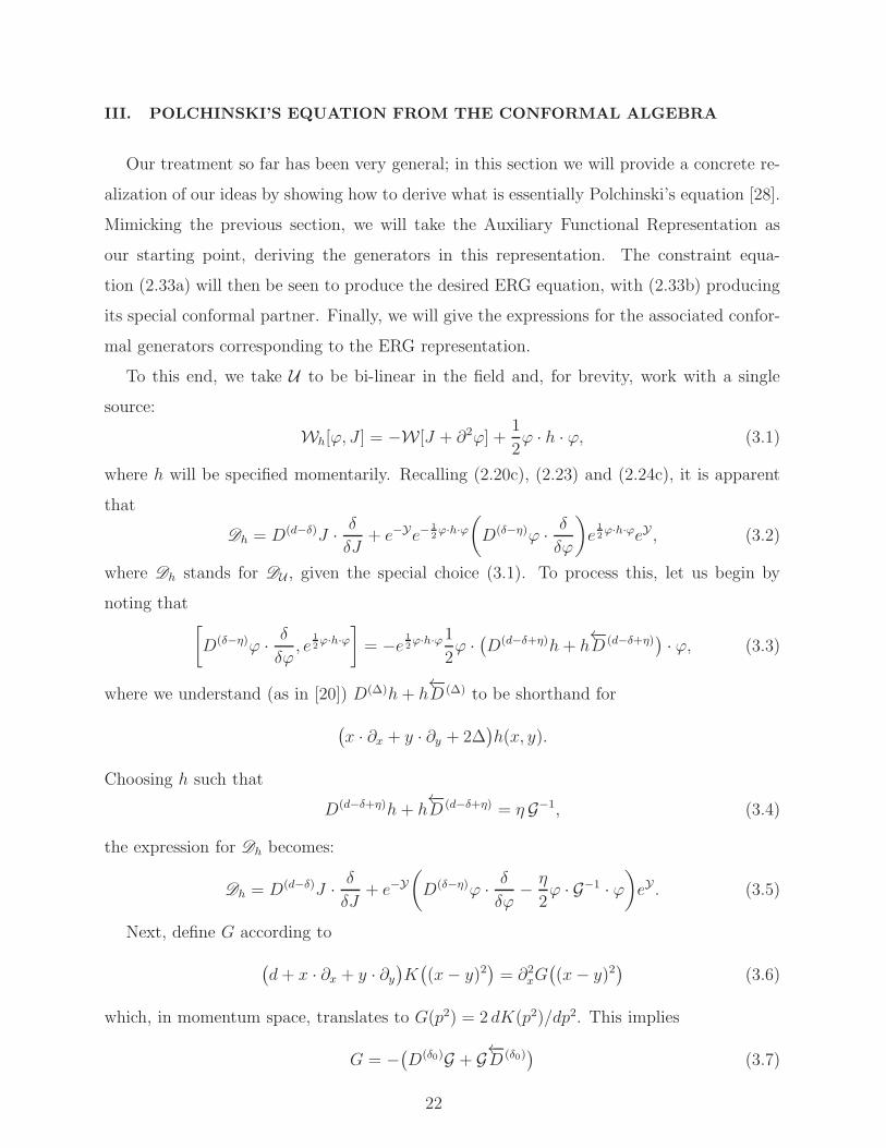
III. POLCHINSKI’S EQUATION FROM THE CONFORMAL ALGEBRA

Our treatment so far has been very general; in this section we will provide a concrete re-

alization of our ideas by showing how to derive what is essentially Polchinski’s equation [28].

Mimicking the previous section, we will take the Auxiliary Functional Representation as

our starting point, deriving the generators in this representation. The constraint equa-

tion (2.33a) will then be seen to produce the desired ERG equation, with (2.33b) producing

its special conformal partner. Finally, we will give the expressions for the associated confor-

mal generators corresponding to the ERG representation.

To this end, we take U to be bi-linear in the field and, for brevity, work with a single

source:

Wh[ϕ, J ] = −W[J + ∂2ϕ] +1

2ϕ · h · ϕ, (3.1)

where h will be specified momentarily. Recalling (2.20c), (2.23) and (2.24c), it is apparent

that

Dh = D(d−δ)J · δδJ

+ e−Ye−1

2ϕ·h·ϕ

(

D(δ−η)ϕ · δδϕ

)

e1

2ϕ·h·ϕeY , (3.2)

where Dh stands for DU , given the special choice (3.1). To process this, let us begin by

noting that[

D(δ−η)ϕ · δδϕ, e

1

2ϕ·h·ϕ

]

= −e 1

2ϕ·h·ϕ1

2ϕ ·

(

D(d−δ+η)h+ h←−D (d−δ+η)

)

· ϕ, (3.3)

where we understand (as in [20]) D(∆)h+ h←−D (∆) to be shorthand for

(

x · ∂x + y · ∂y + 2∆)

h(x, y).

Choosing h such that

D(d−δ+η)h + h←−D (d−δ+η) = η G−1, (3.4)

the expression for Dh becomes:

Dh = D(d−δ)J · δδJ

+ e−Y

(

D(δ−η)ϕ · δδϕ− η

2ϕ · G−1 · ϕ

)

eY . (3.5)

Next, define G according to

(

d+ x · ∂x + y · ∂y)

K(

(x− y)2)

= ∂2xG(

(x− y)2)

(3.6)

which, in momentum space, translates to G(p2) = 2 dK(p2)/dp2. This implies

G = −(

D(δ0)G + G←−D (δ0))

(3.7)

22

from which we observe that

[

e−Y , D(δ−η)ϕ · δδϕ− η

2ϕ · G−1 · ϕ

]

=

(

1

2

δ

δϕ·G · δ

δϕ+ η ϕ · δ

δϕ

)

e−Y (3.8)

where, following the discussion under (2.12), a volume term has been discarded. Substituting

back into (3.5) yields the final expression for the dilatation generator in this representation:

Dh = D(d−δ)J · δδJ

+D(δ)ϕ · δδϕ

+1

2

δ

δϕ·G · δ

δϕ− η

2ϕ · G−1 · ϕ. (3.9)

The constraint equation (2.33a) now yields the ’canonical’ ERG equation, specialized to a

fixed-point:

(

D(d−δ)J · δδJ

+D(δ)ϕ · δδϕ

)

S[ϕ, J ] = 1

2

δSδϕ·G · δS

δϕ− 1

2

δ

δϕ·G · δS

δϕ− η

2ϕ · G−1 · ϕ. (3.10)

An equation like (3.10) was first written down (without sources, but allowing for scale-

dependence) in [29]. It can be thought of as a modification of Polchinski’s equation in which

the anomalous dimension of the fundamental field is explicitly taken into account; see [17, 20]

for detailed analyses. A principle requirement for a valid ERG equation is that the kernels

G and G−1—related via (3.7)—are quasi-local. Typically, G is chosen according to (2.29),

with the cutoff function conventionally normalized so that K(0) = 1 (further details can be

found in [17, 20]). Volume terms, discarded in this paper, are carefully treated in [20].

Deriving the analogous equation arising from special conformal transformations will be

facilitated by the following. For some V(

(x− y)2)

, let us define

Vµ(x, y) ≡ (x+ y)µV(

(x− y)2)

. (3.11)

Proposition 1 Let U(x, y) = U(

(x− y)2)

and suppose that, for some V = V(

(x− y)2)

,

D(∆)U + U←−D (∆) = V.

Then it follows that

K(∆)µU + U

←−K (∆)

µ = Vµ.

Proof: the result follows from the form of D(∆) and K(∆)µ given in (2.4b) and (2.4c).

Applying this result to (3.4), it is apparent that

K(d−δ+η)µh + h

←−K (d−δ+η)

µ = η G−1µ, (3.12)

23

where

G−1µ(x, y) = (x+ y)µG−1

(

(x− y)2))

. (3.13)

Recalling (2.20d), (2.23) and (2.24d), it is apparent that

Khµ = K(d−δ)µJ ·

δ

δJ+ e−Ye−

1

2ϕ·h·ϕ

(

K(δ−η)µϕ ·

δ

δϕ− 2η ∂µϕ · G0 ·

δ

δϕ

)

e1

2ϕ·h·ϕeY . (3.14)

Commuting e1

2ϕ·h·ϕ to the left, the generated of the form ϕ · ∂µG0 · h · ϕ vanishes due to the

asymmetry of ∂µG0 · h under interchange of its arguments. In a little more detail we have,

for some H :

∂µ(G0 · h)(

(x− y)2)

= (x− y)µH(

(x− y)2)

(3.15)

Now,

∫

ddx ddy ϕ(x)(x− y)µH(

(x− y)2)

ϕ(y) = −∫

ddx ddy ϕ(x)(x− y)µH(

(x− y)2)

ϕ(y) = 0,

(3.16)

where in the second step we have swapped the dummy variables x and y. Consequently, we

arrive at the following analogue of (3.5):

Khµ = K(d−δ)µJ ·

δ

δJ+ e−Y

(

K(δ−η)µϕ ·

δ

δϕ− η

2ϕ · G−1

µ · ϕ− 2η ∂µϕ · G0 ·δ

δϕ

)

eY . (3.17)

As before, the strategy is now to commute e−Y to the right. To facilitate this, we note the

following. First, recalling (3.7) and proposition 1 it is apparent that

[

e−Y , K(δ−η)µϕ ·

δ

δϕ

]

eY =1

2

δ

δϕ·Gµ ·

δ

δϕ+η

2

δ

δϕ· Gµ ·

δ

δϕ. (3.18)

Processing the next term in (3.17) gives:

−[

e−Y ,η

2ϕ · G−1

µ · ϕ]

eY = η

(

ϕ · G−1µ · G ·

δ

δϕ− 1

2

δ

δϕ· Gµ ·

δ

δϕ

)

, (3.19)

where we have used the result

G · G−1µ · G = Gµ. (3.20)

This can be seen by reinstating arguments. Equivalently, note that the shorthand for (3.11)

is Vµ = XµV + V Xµ, with(

XµV)

(x, y) = xµV(

(x− y)2)

and(

V Xµ

)

(x, y) = V(

(x− y)2)

yµ,

whereupon it follows that

G · G−1µ · G = G ·XµG−1 · G + G · G−1Xµ · G = GXµ +XµG = Gµ.

24

Finally, the last term in (3.17) gives, on account of translational invariance of G0:

2η

[

e−Y , ∂µϕ · G0 ·δ

δϕ

]

eY = 0 (3.21)

where, in accord with the discussion under (2.30), equality strictly holds only up to a possible

vacuum term. We thus deduce that

Khµ = K(d−δ)µJ ·

δ

δJ+K(δ)

µϕ ·δ

δϕ+

1

2

δ

δϕ·Gµ ·

δ

δϕ− η

2ϕ · G−1

µ· ϕ+ η ϕ · fµ ·

δ

δϕ, (3.22)

where, noticing that the η from the second term’s δ− η has been pulled into the final term,

fµ = G−1µ · G + 2∂µG0 − IXµ −XµI, (3.23)

with I(x, y) = δ(d)(x− y) implying that

(

IXµ +XµI)

(x, y) = (x+ y)µδ(d)(x− y). (3.24)

We now recast fµ in a simpler, manifestly quasi-local form. Recalling that G = G0 ·K and

G−1 = −K−1∂2 it follows that:

G−1µ · G −XµI = −K−1 · ∂2Xµ G0 ·K

= K−1 ·XµK − 2K−1 · ∂µG0 ·K

= K−1 ·XµK − 2∂µG0,

where the last line follows from exploiting G0·K = K ·G0, together with ∂µK ·G0 = −K ·G0←−∂ µ.

Thus, we can simplify:

fµ = K−1 ·[

Xµ, K]

. (3.25)

However,

∂

∂xα

(

(x− y)αK)

=(

d+ x · ∂x − y · ∂x)

K

=(

d+ x · ∂x + y · ∂y)

K = ∂2G (3.26)

where, to go from the first line to the second, we have exploited translational invariance of

K, with the final step following from (3.6). From this, we deduce that

[

Xµ, K]

= ∂µG, (3.27)

25

Therefore, the constraint on the Wilsonian effective action implied by invariance under

special conformal transformations, (2.33b), reads:

(

K(d−δ)µJ ·

δ

δJ+K(δ)

µϕ ·δ

δϕ

)

S[ϕ, J ] =

1

2

δSδϕ·Gµ ·

δSδϕ− 1

2

δ

δϕ·Gµ ·

δSδϕ− η

2ϕ · G−1

µ · ϕ+ η ∂µϕ ·K−1 ·G · δSδϕ. (3.28)

This equation is to the canonical ERG equation (3.10) what Schafer’s equation [14] is to

Wilson’s ERG equation [12].

The generators in the ERG representation are constructed from (3.9) and (3.22) using

the recipe in (2.32c) and (2.32d). The resulting expressions can be simplified by utilising

the constraint equations (3.10) and (3.28).

Representation 5 Canonical ERG representation

Pµ = ∂µJ ·δ

δJ+ ∂µϕ ·

δ

δϕ, (3.29a)

Mµν = LµνJ ·δ

δJ+ Lµνϕ ·

δ

δϕ(3.29b)

D = D(d−δ)J · δδJ

+D(δ)ϕ · δδϕ− δS[ϕ, J ]

δϕ·G · δ

δϕ+

1

2

δ

δϕ·G · δ

δϕ, (3.29c)

Kµ = K(d−δ)µJ ·

δ

δJ+K(δ)

µϕ ·δ

δϕ− δS[ϕ, J ]

δϕ·Gµ ·

δ

δϕ+

1

2

δ

δϕ·Gµ ·

δ

δϕ,

− η ∂µϕ ·K−1 ·G · δδϕ, (3.29d)

where G and Gµ are defined in terms of G via (3.6) and (3.11), the volume terms have been

neglected and S satisfies (3.10) and (3.28).

Though the analysis up to this point has been phrased in terms of conformal primary

fields, we are at liberty to consider non-conformal theories: this can be done simply by

taking the fields to which Ji couple as not being conformal primaries.

26

IV. THE ENERGY-MOMENTUM TENSOR

A. Proposal

Given the scalar, conformal primary field, O (δ), we can furnish a representation of both

this and a partner of scaling dimension d− δ in terms of the appropriate sources:

O(δ)J =

δW[J ]

δJ, (4.1a)

O(d−δ)J = J, (4.1b)

where we recall that the subscript J denotes the Schwinger functional representation. It

is immediately apparent that the pair of fields (4.1a) and (4.1b) satisfy (2.2). However,

satisfaction of (2.2) is a necessary but not sufficient condition for a field to belong to the

spectrum of conformal primaries of a given theory. Indeed, we can construct any number

of solutions to (2.2), but only various combinations of solutions will correspond to the field

contents of actual, realisable theories.

With this in mind, there are two assumptions at play in the statement that O (δ) and

O (d−δ) are conformal primaries. First, it is assumed that W[J ] exists and is non-zero; we

will encounter theories for which one or other of these conditions is violated in subsequent

sections. More subtly, it is assumed that O (d−δ) is amongst the spectrum of fields. As will

be seen in section IVD, if the ERG representation is quasi-local then O (d−δ) is present in

the spectrum as a redundant field.

Note that there are interesting theories for which the assumption that O (d−δ) is in the

spectrum of fields does not hold, in particular the mean field theories. This class of theories

(recently featuring in e.g. [7, 8, 30, 31]) are such that the n-point functions are sums of

products of two-point functions and cannot be represented in terms of a quasi-local action.

The latter restriction amounts to defining mean field theories such as to exclude the Gaussian

theory, plus its quasi-local but non-unitary cousins [17] (see also section IVF); this is done

for terminological convenience. Thus, for mean field theories, (4.1b) amounts to minor

notational abuse since, strictly, O should be reserved for conformal primaries. Accepting

this, we henceforth interpret O(d−δ)J as an object we are at liberty to construct, that in

most—though not all—cases of interest is indeed a conformal primary. A surprising feature

of mean field theories is that the energy-momentum tensor is not amongst the spectrum of

27

conformal primary fields.9

Sticking with the Schwinger functional representation, we construct a scalar field of scaling

dimension d:

O(d)J = −δO (d−δ)

J ×O(δ)J = −δJ × δW[J ]

δJ, (4.2)

where the factor of −δ is inserted so that, at least for theories satisfying the assumptions

given above, we can identify O(d)J with the trace of the energy-momentum tensor. The

× symbol is just to emphasise that no integral is performed. For theories for which the

Schwinger functional exists and is non-zero, but O (d−δ) is not in the spectrum of the fields,

we are again at liberty to construct O(d)J , so long as we accept minor notional abuse and,

more pertinently, that the energy-momentum tensor will not be amongst the spectrum of

conformal primary fields. Recalling the discussion around (1.5), note that (4.2) is nothing

but a statement of the Ward Identity corresponding to dilatation invariance of the Schwinger

functional.

The above can be translated into a representation of our choice, though there is some

subtlety in so doing. Leaving the choice of representation unspecified, let us tentatively

write

O(d) = −δO (d−δ) × O

(δ). (4.3)

Restricting to the Schwinger functional representation clearly just recovers what we had

before. However, there are representations—such as, crucially, the ERG representation—in

which the dilatation and special conformal generators, (3.29c) and (3.29d), are second order

in δ/δϕ. Acting with the dilatation generator, it is generally true that

DO(d) = −δ

(

[

D,O (d−δ)]

×O(δ) + O

(d−δ) ×DO(δ))

. (4.4)

For the Schwinger functional representation which is first order in functional derivatives,

this reduces to

DO(d)J = −δ

(

DO(d−δ)J ×O

(δ)J + O

(d−δ)J ×DO

(δ)J

)

= D(d)O

(d)J . (4.5)

For the ERG representation, as will be seen explicitly in section IVD, the solution is to

extend O(d−δ)loc to O

(d−δ)loc , with the latter such that

[

D, O (d−δ)loc

]

= D(d−δ)O

(d−δ)loc . (4.6)

9 For a non-local two-point theory, η/2 is non-integer [15, 17]. With only two instances of the field and an

even number of derivatives available, it is impossible to construct a local field of dimension, d.

28

With this in mind, we rewrite (4.3) as

O(d) = −δO (d−δ) × O

(δ), (4.7)

with the understanding that for ‘first order’ representations, O (d−δ) just reduces to O (d−δ).

Certain properties which are true of O (d) and its component fields are particularly trans-

parent in the Schwinger functional representation. First of all, observe that, as discussed in

the introduction, translation invariance implies:

∂βO(d−δ)J · O (δ)

J = 0. (4.8)

Integrating by parts it follows that, for some Fαβ ,

O(d−δ)J × ∂βO (δ)

J = −∂αFαβ . (4.9)

Actually, in principle there could be an additional term which cannot be written as a total

derivative but rather vanishes, when integrated, due to the integrand being odd. An example

would be

J(x)

∫

ddy (x− y)βJ(y).

However, such terms are excluded if we insist that the theory in question possesses a quasi-

local representation as we will do, henceforth. Recall that, in a quasi-local representation,

all functions of the field have an expansion in positive powers of derivatives (it is blithely

assumed that this expansion converges). For example, the derivative expansion of the action

reads

S[ϕ] =∫

ddx(

V (ϕ) + Z(ϕ)(∂µϕ)2 + · · ·

)

where V (ϕ) is the local potential which, like Z(ϕ), depends on x only via the field (the ellipsis

represent higher derivative terms). With this in mind, let us consider (4.8) in a quasi-lcoal

representation. Quasi-locality implies that any terms which vanish when integrated must

take the form of total derivatives establishing that, for theories which permit a quasi-local

formulation, (4.9) is correct as it stands. Note that by focussing on theories supporting a

quasi-local representation excludes mean field theories, in particular, from the remainder of

the discussion.

We recognize that the form of (4.9) is that of the Ward Identity associated with con-

servation of the energy-momentum tensor; inspired by this and (4.2) we propose that for

29

theories in which the energy-momentum tensor exists, the Ward Identities can be interpreted

as defining a non-local representation of the energy momentum tensor. Denoting the energy-

momentum tensor in an arbitrary representation—which may or may not be quasi-local—by

Tαβ , we tentatively define this object via10:

Tαα = −δO (d−δ) ×O(δ), (4.10a)

∂αTαβ = −O(d−δ) × ∂βO (δ), (4.10b)

Tαβ = Tβα. (4.10c)

B. Justification

In this section, we justify, for d > 1, the proposal encapsulated in (4.10a), (4.10b)

and (4.10c), which comprises three steps. First it is shown that an object which satis-

fies these equations is implied by translation, rotation and dilatation invariance so long as

Polchinski’s conditions [21] for the improvement of the energy-momentum tensor are sat-

isfied. Secondly, it is shown how both the traceful and longitudinal components of Tαβtransform in a manner consistent with Tαβ being a conformal primary field of dimension

d. Finally, the extent to which (4.10a), (4.10b) and (4.10c) serve to uniquely define Tαβ is

discussed.

1. Existence

The most basic requirement for the existence of a non-null Tαβ , as defined via (4.10a),

(4.10b) and (4.10c), is that the fields O (d−δ) and O (δ) exist and are non-zero. There is some

degree of subtelty here since it is conceivable that O (δ) does not exist in the Schwinger

functional representation but does exist in a quasi-local representation. An example would

be the Gaussian theory in d = 2. The IR behaviour of this theory is sufficiently bad that

the lowest dimension conformal primary is not ϕ but rather ∂µϕ. One method for dealing

with this theory would be to perform the analysis of this section in terms of vector fields.

An alternative, however, is to implicitly work within a quasi-local representation; note that

though O (δ) exists, we are accepting a degree of notational abuse since it is not a conformal

10 Note that since the correlation functions involved in our proposed definition of the energy-momentum

tensor involve only scalar fields, we expect symmetry under interchange of indices.

30

primary in the standard sense. (Later, where more care must be taken, the symbol φ used,

instead). With this in mind, for the duration of this section we assume that at least one

representation of O (d−δ) and O (δ) exists, and at least one of these representations is quasi-

local.

Given this, we now move on to determining the conditions under which (4.10a), (4.10b)

and (4.10c) are implied by a combination of translation, rotation and dilatation invariance.

In section IVA, we have already seen that, for some Fαβ , translation invariance plus the

existence of a quasi-local representation implies (4.9). Similarly, from rotational invariance

it follows that∫

ddx O(d−δ)(x)

(

xα∂β − xβ∂α)

O(δ)(x) = 0. (4.11)

Substituting in (4.9) we have:∫

ddx(

Fαβ(x)− Fβα(x))

= 0, (4.12)

implying that, for some fλαβ, antisymmetric in its last two indices,

Fαβ − Fβα = ∂λfλαβ . (4.13)

We might wonder whether, as in the case of translation invariance, an additional term can

appear on the right-hand side that cannot be expressed as a total derivative. This would be

of the form Yαβ − Yβα, where∫

ddxYαβ is symmetric. Again, quasi-locality guarantees that

such contributions can in fact be absorbed into the total derivative term, ∂λfλαβ .

Inspired by the standard derivation of the Belinfante tensor we observe that, for some

Fλαβ antisymmetric in its first two indices, (4.9) is left invariant by the shift

Fαβ → Fαβ − ∂λFλαβ . (4.14)

Under this transformation, (4.13) becomes:

Fαβ − Fβα = ∂λ(

fλαβ + Fλαβ − Fλβα

)

, (4.15)

and so we choose Fλαβ such that

Fαβ − Fβα = 0. (4.16)

Note that the choice of Fλαβ is not unique: we can add to it further terms, antisymmetric

in the first pair of indices and symmetric in the second, which leave both (4.9) and (4.16)

invariant.

31

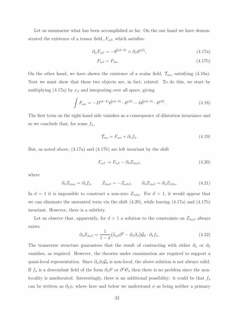
Let us summarize what has been accomplished so far. On the one hand we have demon-

strated the existence of a tensor field, Fαβ , which satisfies:

∂αFαβ = −O(d−δ) × ∂βO (δ), (4.17a)

Fαβ = Fβα. (4.17b)

On the other hand, we have shown the existence of a scalar field, Tαα, satisfying (4.10a).

Next we must show that these two objects are, in fact, related. To do this, we start by

multiplying (4.17a) by xβ and integrating over all space, giving

∫

Fαα = −D(d−δ)O

(d−δ) · O (δ) − δO (d−δ) · O (δ). (4.18)

The first term on the right-hand side vanishes as a consequence of dilatation invariance and

so we conclude that, for some fλ,

Tαα = Fαα + ∂λfλ. (4.19)

But, as noted above, (4.17a) and (4.17b) are left invariant by the shift

Fαβ → Fαβ − ∂λZλαβ , (4.20)

where

∂λZλαα = ∂λfλ, Zλαβ = −Zαλβ , ∂λZλαβ = ∂λZλβα. (4.21)

In d = 1 it is impossible to construct a non-zero Zλβα. For d > 1, it would appear that

we can eliminate the unwanted term via the shift (4.20), while leaving (4.17a) and (4.17b)

invariant. However, there is a subtlety.

Let us observe that, apparently, for d > 1 a solution to the constraints on Zλαβ always

exists:

∂λZλαβ =1

1− d(

δαβ∂2 − ∂α∂β

)

G0 · ∂λfλ. (4.22)

The transverse structure guarantees that the result of contracting with either ∂α or ∂β

vanishes, as required. However, the theories under examination are required to support a

quasi-local representation. Since ∂α∂βG0 is non-local, the above solution is not always valid.

If fλ is a descendant field of the form ∂λO or ∂2Oλ then there is no problem since the non-

locality is ameliorated. Interestingly, there is an additional possibility: it could be that fλ

can be written as ∂λφ, where here and below we understand φ as being neither a primary

32

nor descendant field. This may seem exotic but recall that, for the Gaussian fixed-point in

d = 2, the fundamental field is just such a scalar; indeed, in this case the lowest dimension

primary field is ∂λφ.

Excluding this exotic case, it is clear that the solution (4.22) is no good if fλ is a primary

field. Moreover, it fails for the case that fλ = ∂σfσλ for some fσλ that does not reduce to

δσλ. In d = 2, this is the end of the story, but this is not so for higher dimensionality. Let

us suppose that, for some fσλ

fλ = ∂σfσλ. (4.23)

If fσλ contains the Kronecker-δ then we write fσλ = δσλf . The quasi-local solutions are:

∂λZλαβ =1

2− d(

∂α∂σfσβ + ∂β∂σfσα − ∂2fαβ − δαβ∂σ∂λfσλ)

+1

(2− d)(d− 1)

(

δαβ∂2 − ∂α∂β

)

fσσ for d > 2, (4.24a)

∂λZλαβ =1

1− d(

∂α∂β − δαβ∂2)

f for d = 2. (4.24b)

Observe that these conditions correspond to the recipe found by Polchinski [21] for improving

the energy-momentum tensor of a conformal field theory such that it is traceless.

With these points in mind, consider the sufficient conditions for translation, rotation

and dilatation invariance to imply (4.10a), (4.10b) and (4.10c). In d > 2, absence of a

primary vector field of scaling dimension d− 1 is sufficient. In d = 2 this condition must be

supplemented by at the absence of vector fields that can be written as ∂σfσλ, where fσλ does

not reduce to the Kronecker-δ. In some sense, this is academic since it cannot be realised

for unitary theories. Moreover, as we shall see in section IVC, this additional condition is

relevant only for theories with sufficiently bad IR behaviour.

To conclude this section, let us mention an alternative way to recover Polchinksi’s con-

clusion as to the conditions under which improvement of the energy-momentum tensor is

possible. A version of the analysis below forms a key part of [32], in which an argument is

given as to why scale invariance is automatically enhanced to conformal invariance for the

Ising model in three dimensions.

Using the ‘auxiliary functional representation’ of the conformal algebra: (2.24a)–(2.24d),

consider (2.33a) and (2.33b), supposing that conformal invariance is yet be established but

33

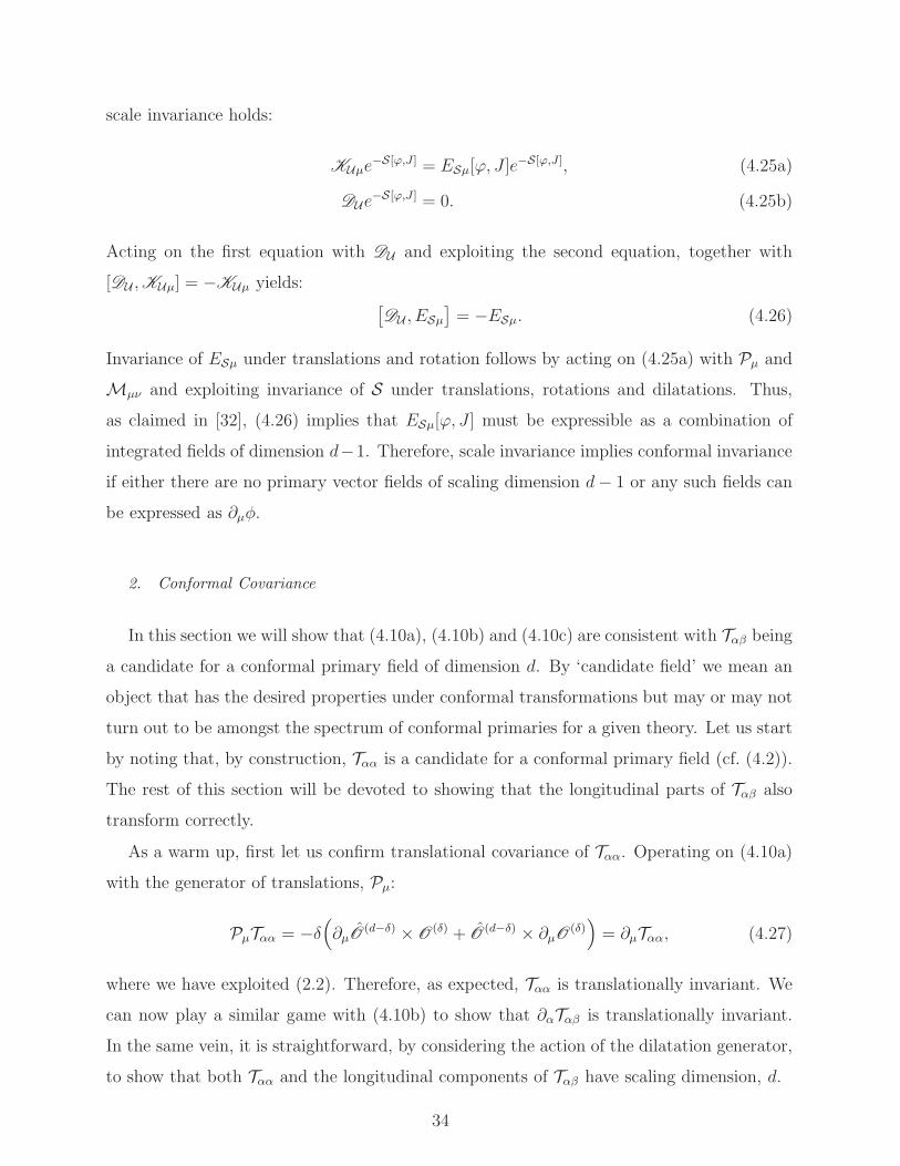
scale invariance holds:

KUµe−S[ϕ,J ] = ESµ[ϕ, J ]e

−S[ϕ,J ], (4.25a)

DUe−S[ϕ,J ] = 0. (4.25b)

Acting on the first equation with DU and exploiting the second equation, together with

[DU ,KUµ] = −KUµ yields:[

DU , ESµ

]

= −ESµ. (4.26)

Invariance of ESµ under translations and rotation follows by acting on (4.25a) with Pµ and

Mµν and exploiting invariance of S under translations, rotations and dilatations. Thus,

as claimed in [32], (4.26) implies that ESµ[ϕ, J ] must be expressible as a combination of

integrated fields of dimension d−1. Therefore, scale invariance implies conformal invariance

if either there are no primary vector fields of scaling dimension d− 1 or any such fields can

be expressed as ∂µφ.

2. Conformal Covariance

In this section we will show that (4.10a), (4.10b) and (4.10c) are consistent with Tαβ being

a candidate for a conformal primary field of dimension d. By ‘candidate field’ we mean an

object that has the desired properties under conformal transformations but may or may not

turn out to be amongst the spectrum of conformal primaries for a given theory. Let us start

by noting that, by construction, Tαα is a candidate for a conformal primary field (cf. (4.2)).

The rest of this section will be devoted to showing that the longitudinal parts of Tαβ also

transform correctly.

As a warm up, first let us confirm translational covariance of Tαα. Operating on (4.10a)

with the generator of translations, Pµ:

PµTαα = −δ(

∂µO(d−δ) × O

(δ) + O(d−δ) × ∂µO (δ)

)

= ∂µTαα, (4.27)

where we have exploited (2.2). Therefore, as expected, Tαα is translationally invariant. We

can now play a similar game with (4.10b) to show that ∂αTαβ is translationally invariant.

In the same vein, it is straightforward, by considering the action of the dilatation generator,

to show that both Tαα and the longitudinal components of Tαβ have scaling dimension, d.

34

Covariance of Tαα under rotations and special conformal transformations follows exactly

the same pattern. Dealing with (4.10b) is only ever so slightly more involved. To start with,

let us consider rotations:

Mµν∂αTαβ = −LµνO(d−δ)∂βO

(d) − O(d−δ)∂βLµνO

(d)

= Lµν∂αTαβ + δµβ∂αTαν − δνβ∂αTαµ. (4.28)

Now, given a symmetric conformal primary tensor field, O(d)αβ , let us compare (4.28) with

∂αO(d)αβ , the result of which we can compute using (2.5a):

Mµν∂αO(d)αβ = ∂α

(

LµνO(d)αβ +

(

δµαδλν − δναδλµ)

O(d)λβ +

(

δµβδλν − δνβδλµ)

O(d)αλ

)

= Lµν ∂αO(d)αβ + δµβ∂αO

(d)αν − δνβ∂αO

(d)αµ . (4.29)

Comparing (4.28) and (4.29), we conclude that the longitudinal pieces of Tαβ transform

under rotations like a conformal primary tensor field.

Finally, we deal with special conformal transformations:

Kµ∂αTαβ = −K(d−δ)µO

(d−δ)∂βO(δ) − O

(d−δ)∂βK(δ)

µO(δ)

= K(d)µ∂αTαβ + 2δµβ

(

xλ∂αTαλ + Tαα)

+ 2xµ∂αTαβ − 2xβ∂αTαµ. (4.30)

Now, given a symmetric conformal primary tensor field, O(d)αβ , let us compare (4.30) with

Kµ∂αO(d)αβ , the result of which we can compute using (2.5b). Exploiting symmetry under

α↔ β it is straightforward to show that

Kµ∂αO(d)αβ = K(d)

µ∂αO(d)αβ + 2δµβ

(

xλ∂αO(d)αλ + O

(d)αα

)

+ 2xµ∂αO(d)αβ − 2xβ∂αO

(d)αµ . (4.31)

Comparing (4.30) and (4.31) it is apparent that the longitudinal pieces of Tαβ transforms

under conformal transformations like a conformal primary tensor field of dimension d.

3. Uniqueness

A two-index tensor has d2 a priori independent components. The condition of symmetry

under interchange of indices imposes d(d− 1)/2 constraints; conservation imposes a further

d, whereas (4.10a) yields one additional constraint. This reduces the number of independent

components to(d− 2)(d+ 1)

2.

35

Immediately it is apparent that (4.10a), (4.10b) and (4.10c) uniquely define the energy-

momentum tensor in d = 2.

For d > 2, we must accept that, in general, Tαβ is not uniquely defined. Notice that the

equations (4.10a), (4.10b) and (4.10c) are invariant under

Tαβ → Tαβ + Zαβ, (4.32)

where

Zαα = 0, ∂αZαβ = 0, Zαβ = Zβα. (4.33)

The results of the previous sub-section show that the traceful and longitudinal compo-

nents of Tαβ transform as expected for a conformal primary of dimension d. Let us now focus

on conformal field theories for which the energy-momentum tensor exists. We assume that

Zαβ is chosen such that any remaining components of Tαβ also transform homogeneously.

However, this still leaves a residual freedom to add to Zαβ a contribution, Zαβ, which also

transforms like a conformal primary of dimension d. This requirement, together with (4.33),

implies that [33]:

Zαβ = ∂ρ∂σCαρβσ, (4.34)

where Cαρσβ is a conformal primary field of dimension d − 2 with the same symmetries as

the Weyl tensor:

Cαρβσ = −Cραβσ = −Cαρσβ ,

Cαρβσ + Cαβσρ + Cασρβ = 0,

Cαρασ = 0.

(4.35)

For d = 3, these constraints do not have a non-trivial solution and so extend the uniqueness

of the energy-momentum, for a conformal field theory, to this dimensionality. Beyond this,

uniqueness or otherwise depends on whether or not the theory in question supports Cαρβσ

as a conformal primary field of dimensions d− 2 [33].

Though we will not rely on the following restriction in this paper, it is expected that

the energy-momentum tensor is unique for unitary theories.11 In d = 4, Cαρβσ transforms

under the (2, 0) ⊕ (0, 2) representation. However, Mack rigorously established that for a

representation of type (j, 0), unitarity demands that the scaling dimension ∆ > 1 + j [34].

11 I would like to thank H. Osborn for informing me of this and for providing the argument as to why.

36

This implies that the scaling dimension of ∂ρ∂σCαρβσ is greater than five and so this field

cannot contribute to the energy-momentum tensor which, in the considered dimensionality,

is of scaling dimension four. A similar result is expected to hold in higher dimensions.

C. Conformal Invariance

We have previously established the conditions under which (4.10a), (4.10b) and (4.10c)

hold. Given these equations, it is a simple matter to demonstrate conformal invariance

(indeed, we have essentially shown that the energy-momentum tensor can be improved to a

traceless, symmetric form). Recall that the condition for conformal invariance reads:

K(d−δ)µJ ·

δW[J ]

δJ= 0 (4.36)

which, in an arbitrary representation, becomes:

K(d−δ)µO

(d−δ) · O (δ) = 0, ⇒ O(d−δ) ·K(δ)

µO(δ) = 0. (4.37)

With this in mind, consider a theory for which full conformal invariance is yet to be estab-

lished. Utilizing (4.10a), (4.10b) and (4.10c), we see that

O(d−δ) ·K(δ)

µO(δ) = O

(d−δ) ·(

2xµ(x · ∂ + δ)− x2∂µ)

O(δ)

=

∫

ddx(

x2∂αTαµ − 2xµxβ∂αTαβ − 2xµTαα)

= 2

∫

ddxxα(

Tµα − Tαµ)

= 0 (4.38)

where, to go from the second to third lines we have integrated by parts, and to go to the last

line we have exploited symmetry of Tµα under interchange of indices. Therefore, conformal

invariance has been demonstrated.

It is interesting to consider theories for which the energy-momentum tensor cannot be

improved to be traceless. According to (4.19), there is a residual term of the form ∂λfλ

which spoils conformal invariance. Repeating the analysis of (4.38), it is apparent that

O(d−δ) ·K(δ)

µO(δ) ∝

∫

ddx fµ. (4.39)

The intriguing thing about this condition is that, in d = 2, the sufficient conditions for the

improvement of the energy-momentum tensor include the absence of a vector field which can

37

be written as ∂σfσλ, where fσλ does not reduce to the Kronecker-δ. However, suppose that

fµ can be written in this fashion; according to (4.39), conformal invariance is present since

the right-hand side vanishes! This apparent paradox is resolved by noting that, in the quasi-

local representation appropriate to the discussion of the improvement energy-momentum

tensor, O (d−δ) ·K(δ)µO

(δ) = 0 does not quite imply conformal invariance of the correlation

functions: this only holds if W[J ] exists, which it will not if the IR behaviour is sufficiently

bad. This will be exemplified in section IVF by a non-unitary theory.

D. Quasi-Local Representation

The defining equations for the energy-momentum tensors, (4.10a), (4.10b) and (4.10c)

are independent of any particular representation. As already apparent, a prominent role

is played by the Schwinger functional representation; the other representation of particular

interest is furnished by the ERG, which provides a quasi-local framework. For the sake of

definiteness, in this section we will explore the energy-momentum tensor using the canon-

ical ERG equation, discussed in section III. Recall that δ can be written in terms of the

anomalous dimension of the fundamental via (2.19).

In this context, we have:

O(δ)loc = K−1 ·

(

1 + )

· ϕ+ G0 · ·δSδϕ, (4.40a)

O(d−δ)loc = ϕ · G−1

0 +δSδϕ·K, (4.40b)

where, in momentum space, for η < 2

(p2) = −p2(η/2)K(p2)

∫ p2

0

dq2[

1

K(q2)

]′

q−2(η/2), (4.41)

with K the momentum-space cutoff introduced in (2.29). The expressions for and O (δ)

first appeared in [35] and played a prominent role in much of the analysis of [17]. The pair

of fields (4.40a) and (4.40a) appears in both [17, 20]. Note that the h appearing in (3.1) is

(given appropriate boundary conditions) related to according to [17]:

h = G−1 ·(

1l + )

+ h0, h0 =

{

1, η = 0,

0, η < 2, 6= 0.(4.42)

For our purposes, though, we seek a slight modification to O(d−δ)loc , as discussed around

(4.3). To motivate this, consider (4.7). The novelty of the current representation is that the

38

dilatation generator (3.29c) has a term containing not one but two functional derivatives.

Consequently,

DS [ϕ]O 6=[

DS [ϕ],O]

.

Therefore, we seek an extension of O(d−δ)loc , to be denoted O

(d−δ)loc , such that

[

DS [ϕ], O(d−δ)loc

]

= D(d−δ)O

(d−δ)loc . (4.43)

In this way we can construct

O(d)loc = −δO (d−δ)

loc × O(δ)loc , (4.44)

which by construction satisfies

DS [ϕ]O(d)loc = D(d)

O(d)loc . (4.45)

The solution is to take

O(d−δ)loc = ϕ · G−1

0 +δSδϕ·K − δ

δϕ·K. (4.46)

There a various ways to obtain this equation. On the one hand, a brute force calculation

can be performed, along the lines of appendix C of [17]. However, there is a more elegant

approach. Notice that we may write

O(d−δ)loc = eSe−Y ϕ · G−1

0 eYe−S . (4.47)

Recalling (2.31) and (3.5), it is apparent that

[

DS [ϕ], O(d−δ)loc

]

= eSe−Y D(δ−η)ϕ · G−10 eYe−S . (4.48)

Splitting δ − η = δ0 − η/2 and noting that

D(d−δ0)G−10 + G−1

0

←−D (d−δ0) = 0, (4.49)

it follows that

D(δ−η)ϕ · G−10 = −η

2ϕ · G−1

0 − ϕ ·D(d−δ0)G−10

= −η2ϕ · G−1

0 + ϕ · G−10

←−D (d−δ0)

= ϕ · G−10

←−D (d−δ), (4.50)

confirming (4.43).

39

As we know from (4.10a), the fields discussed above can be combined to form the trace of

the energy-momentum tensor. Integrating over space, we recognize the resulting object as

nothing other than the exactly marginal, redundant field which exists at every critical fixed-

point. Recall that the definition of a redundant field is that it can be cast as a quasi-local field

redefinition. This is essentially manifest in the case of the trace of the energy-momentum

tensor—which in the ERG representation we denote by Tαα—since∫

Tαα = −δO (d−δ)loc · O (δ)

loc

= −δeS[ϕ](

δ

δϕ− ϕ · G−1

)

·(

G · · δδϕ−

(

1 + )

· ϕ)

e−S[ϕ]. (4.51)

Recalling (2.37) we have, for infinitesimal ǫ:

e−Stot[ϕ]+ǫ∫Tαα =

{

1− ǫδ δδϕ·(

G · · δδϕ− ϕ

)}

e−Stot[ϕ]. (4.52)

On account of the total functional derivative on the right-hand side, it follows that the

partition function is invariant under an infinitesimal shift of the action in the direction of

the (integrated) trace of the energy-momentum tensor; in standard parlance, this field is

redundant.

It has been appreciated for a long time that every critical fixed-point solution of the ERG

equation in fact exists as a line of physically equivalent fixed-points [15–17, 24, 25]. The

exactly marginal, redundant field generates infinitesimal motion along this line: if the line

is parametrized by b, then

S(b+ δb) = S(b) + δbO (d−δ) · O (δ). (4.53)

For the canonical ERG equation, a generic expression for the entire line of fixed-points can

be found in [17] (see also [36, 37]). Within the ERG formalism, it has been shown that

for any (quasi-local) fixed-point for which the exactly marginal, redundant field exists, the

value of η is isolated [17] (the converse was proven in [15]). From the perspective of this

paper, this property can now be understood as arising for quasi-local theories for which the

(trace of the) energy-momentum tensor exists and is non-zero.

E. The Gaussian Fixed-Point

An instructive illustration of many of the concepts discussed above is provided by the

Gaussian fixed-point, which describes a free theory for which the fundamental field has scal-

40

ing dimension δ = δ0 = (d−2)/2. Before providing the canonical ERG representation of this

theory, we will derive the expression for the energy-momentum tensor in the para-Schwinger

functional representation. We do this since, for the special case of the Gaussian fixed-point,

this representation is, in fact, strictly local and, as such, equivalent to an unregularized ac-

tion approach. Consequently, this should provide a familiar setting prior to our exposition of

the less conventional ERG approach. Note that the difference between O (d−δ0) and O (d−δ0)

amounts only to a vacuum term, which we ignore (the same is true in section IVF).

1. Para-Schwinger Functional Representation

In this representation, (and employing canonical normalization) we have O (d−δ0) = −∂2ϕand O (δ0) = ϕ, from which we observe that:

−∂2ϕ× ∂βϕ = −∂α(

∂αϕ× ∂βϕ)

− 1

2∂β(

∂λϕ× ∂λϕ)

= −∂α(

∂αϕ× ∂βϕ−1

2δαβ∂λϕ× ∂λϕ

)

. (4.54)

Upon comparison with (4.10b), and using a tilde to denote the para-Schwinger functional

representation, it is apparent that:

Tαβ = ∂αϕ× ∂βϕ−1

2δαβ∂λϕ× ∂λϕ+

δ0d− 1

∂λZλαβ , (4.55)

where Zλαβ(ϕ) satisfies the conditions (4.21) but is thus far undetermined; the factor of

δ0/(d− 1) has been inserted for convenience. Taking the trace and comparing with (4.10a):

− d− 2

2∂λϕ× ∂λϕ+

δ0d− 1

∂λZλαα = δ0∂2ϕ× ϕ. (4.56)

This is solved by taking

∂λZλαβ =(

δαβ∂2 − ∂α∂β

)1

2ϕ2, (4.57)

yielding the standard Gaussian energy-momentum tensor:

Tαβ = ∂αϕ× ∂βϕ−1

2δαβ∂λϕ× ∂λϕ +

d− 2

4(d− 1)

(

δαβ∂2 − ∂α∂β

)

ϕ2. (4.58)

Before moving on, it is instructive to consider the expression for the energy-momentum

tensor in the Schwinger functional representation. Recalling (1.2) and (2.15), this can be

obtained from (4.58) simply by making the substitution

ϕ→ −G0 · J. (4.59)

41

It is thus apparent that, in the Schwinger functional representation,

∂αTαβ = −J × ∂βG0 · J, (4.60a)

Tαα = −δ0J × G0 · J, (4.60b)

precisely as we expect for the Ward identities involving the connected correlator of the

Gaussian theory.

2. ERG Representation

In the ERG formalism, the Gaussian theory exhibits a line of physically equivalent

fixed-points, as expected, which terminates in a non-critical fixed-point for which both the

Schwinger functional vanishes and the energy-momentum tensor vanish. The Gaussian so-

lution of the canonical ERG equation is (in momentum space):

S[ϕ] = 1

2

∫

p

ϕ(p)bp2

1− bK(p2)ϕ(−p), Stot[ϕ] =

1

2

∫

p

ϕ(p)p2K−1(p2)

1− bK(p2)ϕ(−p), (4.61)

where, in accord with convention, K(0) = 1 and∫

p≡ (2π)−d

∫

ddp . It is thus apparent

that the Gaussian fixed point exists as a line for −∞ < b < 1. At b = 1, the action is

still a fixed-point in the sense of solving the ERG equation. However, Taylor expanding

K(p2) = 1 + O(

p2)

, it is clear that the action does not describe a theory with long-range

order: this theory is non-critical. As emphasised by Wegner, such theories support only

redundant fields and, as we will see below, both the energy-momentum tensor and the

correlation functions vanish. Note that, for b > 1, the coefficient of ϕ(p)p2ϕ(−p) turns

negative, which manifests itself as a loss of positivity of the two-point correlation function,

as will also be seen below.

Defining

G = (1− bK)−1, (4.62)

the Gaussian solution can be rewritten:

Stot[ϕ] =1

2ϕ · G−1 ·G · ϕ. (4.63)

Substituting into (4.40a) and (4.46), it can readily be confirmed that

O(δ)loc = (1− b)G · ϕ, (4.64a)

O(d−δ)loc = ϕ ·G · G−1

0 . (4.64b)

42

The full energy-momentum tensor can be obtained from (4.58) by making the substitution

ϕ(x)→√1− b

∫

ddy G(

(x− y)2)

ϕ(y). (4.65)

Furthermore, as shown explicitly in [17], the Schwinger functional for the Gaussian theory

is given by

W[J ] =1− b2

∫

p

J(p)1

p2J(−p). (4.66)

Thus it is apparent that, at the point the theory turns non-critical, both the correlation

functions and the energy-momentum tensor vanish. For b > 1, positivity of the two-point

function is violated.

F. A Non-Unitary Example

Having observed the successful construction of the energy-momentum tensor in the sim-

plest local, unitary theory, in this section we will provide a simple non-unitary example

where the construction breaks down—at least in d = 2. (For a pedagogical exposition of

various aspects of unitarity, see [38].) Specifically, we will consider a free theory for which

η = −2.In momentum space, it is a simple matter to show that [17]

S =1

2

∫

p

ϕ(p)ϕ(−p)bp2 − p4K−1(1 + )

p2 − bK , (4.67)

where b parametrizes the line of equivalent fixed-points and is given by (4.41). Note that

the two-point function for the full action, cf. (2.37), starts at O(

p4)

. It follows that

O(δ)(p) = − b

p2− bKϕ(p), (4.68a)

O(d−δ)(p) = − p4

p2 − bKϕ(p). (4.68b)

Taking b = −1 (to attain canonical normalization) let us define

Φ = (p2+K)−1 · ϕ, (4.69)

giving O (d−δ) = −∂4Φ and O (δ) = Φ. The attempted construction of the energy-momentum

tensor precedes in a similar vein to before. Observe that

∂αΦ× ∂4Φ = ∂ρ(

∂αΦ× ∂ρ∂2Φ+ ∂ρΦ× ∂α∂2Φ)

− 1

2∂α

(

∂2Φ× ∂2Φ+ 2∂ρΦ× ∂ρ∂2Φ)

. (4.70)

43

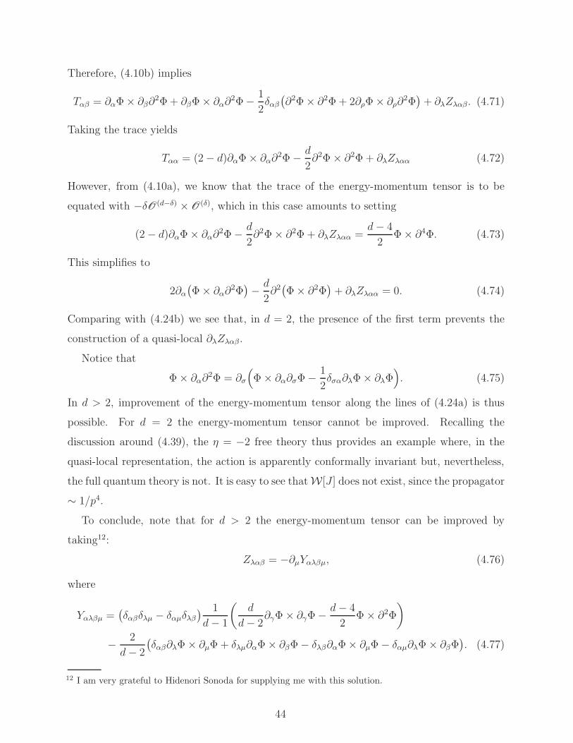
Therefore, (4.10b) implies

Tαβ = ∂αΦ× ∂β∂2Φ+ ∂βΦ× ∂α∂2Φ−1

2δαβ

(

∂2Φ× ∂2Φ+ 2∂ρΦ× ∂ρ∂2Φ)

+ ∂λZλαβ. (4.71)

Taking the trace yields

Tαα = (2− d)∂αΦ× ∂α∂2Φ−d

2∂2Φ× ∂2Φ + ∂λZλαα (4.72)

However, from (4.10a), we know that the trace of the energy-momentum tensor is to be

equated with −δO (d−δ) × O (δ), which in this case amounts to setting

(2− d)∂αΦ× ∂α∂2Φ−d

2∂2Φ× ∂2Φ + ∂λZλαα =

d− 4

2Φ× ∂4Φ. (4.73)

This simplifies to

2∂α(

Φ× ∂α∂2Φ)

− d

2∂2(

Φ× ∂2Φ)

+ ∂λZλαα = 0. (4.74)

Comparing with (4.24b) we see that, in d = 2, the presence of the first term prevents the

construction of a quasi-local ∂λZλαβ.

Notice that

Φ× ∂α∂2Φ = ∂σ

(

Φ× ∂α∂σΦ−1

2δσα∂λΦ× ∂λΦ

)

. (4.75)

In d > 2, improvement of the energy-momentum tensor along the lines of (4.24a) is thus

possible. For d = 2 the energy-momentum tensor cannot be improved. Recalling the

discussion around (4.39), the η = −2 free theory thus provides an example where, in the

quasi-local representation, the action is apparently conformally invariant but, nevertheless,

the full quantum theory is not. It is easy to see thatW[J ] does not exist, since the propagator

∼ 1/p4.

To conclude, note that for d > 2 the energy-momentum tensor can be improved by

taking12:

Zλαβ = −∂µYαλβµ, (4.76)

where

Yαλβµ =(

δαβδλµ − δαµδλβ) 1

d− 1

(

d

d− 2∂γΦ× ∂γΦ−

d− 4

2Φ× ∂2Φ

)

− 2

d− 2

(

δαβ∂λΦ× ∂µΦ + δλµ∂αΦ× ∂βΦ− δλβ∂αΦ× ∂µΦ− δαµ∂λΦ× ∂βΦ)

. (4.77)

12 I am very grateful to Hidenori Sonoda for supplying me with this solution.

44

By virtue of the symmetries

Yαλβµ = −Yλαβµ = Yβµαλ, (4.78)

it is apparent that, as required,

∂α∂λZλαβ = 0, ∂λZλαβ = ∂λZλβα. (4.79)

Finally, it can be checked that, upon taking the trace, we recover (4.74).

V. CONCLUSIONS

The essence of the philosophy advocated in this paper is a conservative one. At its heart is

the desire to view, as far as possible, QFT as fundamental. (Whether or not this ultimately

turns out to be the case is beside the point; the goal is partly to see how far one can go

by pursuing this agenda.) Taking this seriously, we are driven to look for theories which

make sense down to arbitrarily short distances (i.e. theories exhibiting non-perturbative

renormalizability). Wilsonian renormalization teaches us that a sufficient condition for this

is scale-invariant behaviour in the deep UV, suggesting that we investigate either fully scale-

invariant theories or relevant/marginally relevant deformations, thereof.

Our exclusive focus has been on theories exhibiting invariance under the full conformal

group. In this context, there are two largely disjoint approaches: one based on exploring

the constraints implied by conformal invariance on the correlation functions and the other a

path integral approach built upon a quasi-local action. True to our philosophy, the former

is viewed as more primitive due to its inherently quantum field-theoretic nature whereas,

through the action, the latter manifests its classical heritage. Ideally, then, what we would

like is to be able to start with an approach based on the correlation functions and to show

how an action-based description emerges.

This paper largely shows how to achieve this. Starting from the statements of conformal

covariance of the correlation functions, the first step is to wrap these up into functionals of

sources (accepting a degree of formality in this step). Associated with this is a functional

representation of the conformal algebra. This forms the basis for constructing more elab-

orate representations, involving auxiliary functionals. These auxiliary functionals satisfy

consistency conditions, and our development culminated with a representation in which the

condition corresponding to dilatation invariance is nothing but the fixed-point version of the

45

canonical ERG equation of [29]. The explicit form of the partner encoding special conformal

invariance is a new result of this paper.

Nevertheless, it must be acknowledged that we were guided towards this representation

because we knew what we were looking for. This, in of itself, is not an issue. More pressing is

that, coming from the path integral perspective, it is expected that all physically acceptable

solutions to ERG equations correspond to quasi-local actions [12, 17]. The step that is

missing in this paper is to show that ERG representations of CFTs necessarily have a

Wilsonian effective action that is, indeed, quasi-local. Or, to put it another way, of all the

possible representations of the conformal algebra, what makes the ERG representation so

special? Suggestively, as alluded to in section IVD, if the ERG representation of a CFT

is quasi-local, then the energy-momentum tensor is amongst the spectrum of conformal

primaries. Indeed, the ERG and the energy-momentum tensor share an intimate relationship

revealed in this paper: lines of physically equivalent fixed-points are generated by the trace

of the energy-momentum tensor.

Therefore, referring to the questions posed in the introduction, the state of affairs is

as follows. A concrete recipe has been provided for encoding conformal dynamics in an

object recognizable as the Wilsonian effective action. This assumes (2.22) which, given the

choice (2.28), amounts to an assumption of the existence of a path integral. As noted, in

d = 2 it may be necessary to work in finite volume. Plausibly, the rather formal process

presented will work for theories possessing an energy-momentum tensor, in which case we

expect the Wilsonian representation to furnish a quasi-local formulation of the theory in

question. It is clearly desirable, however, to place all of this on a more rigorous footing.

Beyond this matter, it is worth posing the question as to whether there may exist theories

supporting representations of the conformal algebra for which the constraint which picks out

physically acceptable theories is entirely different from quasi-locality, but equally powerful.

Besides exploring this theme further, several avenues of future research suggest themselves.

Transcribing our approach to supersymmetric theories should be largely a matter of working

with the appropriate potential superfields, as in [39], and being mindful that the conformal

algebra is enhanced to be superconformal. A controlled environment in which to further

explore the CFT/ERG link is in d = 2, where is may be profitable to investigate functional

representations of the entire Virasoro algebra. As indicated earlier, a rigorous treatment

in d = 2 may entail a careful finite-volume treatment. Gauge theories present special

46

problems [17, 40] and it is my belief that appropriately extending the ideas of this paper

will require new ideas.

Furthermore, it is desirable to extend the scope of the analysis to include scale-dependent

theories. It is anticipated that the renormalizability (or otherwise) of such theories is tied up

with the renormalization of composite operators. Since, for irrelevant/marginally irrelevant

perturbations, renormalizability is lost this suggests that, in order to properly define the

fixed-point Schwinger functional involving the corresponding sources, some form of point

splitting should be performed on the composite operators, to improve their UV behaviour.

It may be that this engenders a natural way to uncover the operator product expansion

within the ERG formalism, raising the hope of making concrete links between the ideas of

this paper and recent developments in the application of the conformal bootstrap.

Finally, it is worth considering the question as to whether theories exist in which there are

multiple, distinct quasi-local representations. This leads naturally to the subject of dualities

and it is hoped that the ideas of this paper and the fresh perspective it gives on the nature

and origins of Wilsonian renormalization will offer new insights in this area.

ACKNOWLEDGMENTS

This paper is dedicated to the memory of my friend, Francis Dolan, who died, tragically,

in 2011. It is gratifying that I have been able to honour him with work which substantially

overlaps with his research interests and also that some of the inspiration came from a long

dialogue with his mentor and collaborator, Hugh Osborn. In addition, I am indebted to Hugh

for numerous perceptive comments on various drafts of the manuscript and for bringing to my

attention gaps in my knowledge and holes in my logic. I would like to thank Yu Nakayama

and Hidenori Sonoda for insightful correspondence following the appearance of the first and

third versions on the arXiv, respectively.

I am firmly of the conviction that the psychological brutality of the post-doctoral system

played a strong underlying role in Francis’ death. I would like to take this opportunity,

should anyone be listening, to urge those within academia in roles of leadership to do far more

to protect members of the community suffering from mental health problems, particularly

47

during the most vulnerable stages of their careers.

[1] F. A. Dolan and H. Osborn, “Conformal four point functions and the operator product ex-

pansion,” Nucl. Phys. B 599 (2001) 459, hep-th/0011040.

[2] F. A. Dolan and H. Osborn, “Conformal partial waves and the operator product expansion,”

Nucl. Phys. B 678 (2004) 491, hep-th/0309180.

[3] F. A. Dolan and H. Osborn, “Conformal Partial Waves: Further Mathematical Results,”

arXiv:1108.6194 [hep-th].

[4] R. Rattazzi, S. Rychkov, E. Tonni, and A. Vichi, “Bounding scalar operator dimensions in 4D

CFT,” JHEP 0812 (2008) 31, arXiv:0807.0004 [hep-th].

[5] M. S. Costa, J. Penedones, D. Poland, and S. Rychkov, “Spinning Conformal Blocks,” JHEP

1112 (2011) 154, arXiv:1109.6321 [hep-th].

[6] D. Poland and D. Simmons-Duffin, “Bounds on 4D Conformal and Superconformal Field

Theories,” JHEP 1105 (2011) 017, arXiv:1009.2087 [hep-th].

[7] S. El-Showk, M. F. Paulos, D. Poland, S. Rychkov, D. Simmons-Duffin, and A. Vichi, “Solv-

ing the 3d Ising Model with the Conformal Bootstrap,” Phys. Rev. D 86 (2012) 025022,

arXiv:1203.6064 [hep-th].

[8] S. El-Showk, M. F. Paulos, D. Poland, S. Rychkov, D. Simmons-Duffin, and A. Vichi, “Solving

the 3d Ising Model with the Conformal Bootstrap II. c-Minimization and Precise Critical

Exponents,” arXiv:1403.4545 [hep-th].

[9] F. Gliozzi, “More constraining conformal bootstrap,” Phys. Rev. Lett. 111 (2013) 161602,

arXiv:1307.3111 [hep-th].

[10] F. Gliozzi and A. Rago, “Critical exponents of the 3d Ising and related models from Conformal

Bootstrap,” JHEP 1410 (2014) 42, arXiv:1403.6003 [hep-th].

[11] A. A. Belavin, A. M. Polyakov, and A. B. Zamolodchikov, “Infinite conformal symmetry in

two-dimensional quantum field theory,” Nucl. Phys. B 241 (1984) 333.

[12] K. G. Wilson and J. Kogut, “The Renormalization group and the epsilon expansion,” Phys.

Rept. 12 (1974) 75.

[13] T. R. Morris, “The Exact renormalization group and approximate solutions,” Int. J. Mod.

Phys. A 9 (1994) 2411, hep-ph/9308265.

48

[14] L. Schafer, “Conformal Covariance in the Framework of Wilson’s Renormalization Group

Approach,” J. Phys. A 9 (1976) 377–395.

[15] F. J. Wegner, “The Critical State, General Aspects,” in Phase Transitions and Critical Phe-

nomena, Vol.6, C. Domb and M. S. Green, eds., p. 7. London, 1976.

[16] T. R. Morris, “Elements of the continuous renormalization group,” Prog. Theor. Phys. 131

(1998) 395, hep-th/9802039.

[17] O. J. Rosten, “Fundamentals of the Exact Renormalization Group,” Phys. Rept. 511 (2012)

177, arXiv:1003.1366 [hep-th].

[18] T. R. Morris, “The Renormalization group and two-dimensional multicritical effective scalar

field theory,” Phys. Lett. B 345 (1995) 139, hep-th/9410141.

[19] F. Di Francesco, P. Mathieu, and D. Senechal, Conformal Field Theory. Springer, 1997.

[20] H. Osborn and D. E. Twigg, “Remarks on Exact RG Equations,” Annals Phys. 327 (2012)

29, arXiv:1108.5340 [hep-th].

[21] J. Polchinski, “Scale and Conformal Invariance in Quantum Field Theory,” Nucl. Phys. B

303 (1988) 226.

[22] A. B. Zamolodchikov, “Irreversibility of the Flux of the Renormalization Group in a 2D Field

Theory,” JETP Lett. 43 (1986) 730 [Pisma Zh. Eksp. Teor. Fiz. 43, 565 (1986)].

[23] Y. Nakayama, “A lecture note on scale invariance vs conformal invariance,”

arXiv:1302.0884 [hep-th].

[24] F. J. Wegner, “Some Invariance Properties of the Renormalization Group,” J. Phys C 7 (1974)

2098.

[25] E. Riedel, G. R. Golner, and K. E. Newman, “Scaling Field Representation Of Wilson’s Exact

Renormalization Group Equation,” Annals Phys. 161 (1985) 178.

[26] O. J. Rosten Work in progress.

[27] J. L. Latorre and T. R. Morris, “Exact scheme independence,” JHEP 0011 (2000) 004,

hep-th/0008123.

[28] J. Polchinski, “Renormalization And Effective Lagrangians,” Nucl. Phys. B 231 (1984) 269.

[29] R. D. Ball, P. E. Haagensen, J. I. Latorre, and E. Moreno, “Scheme Independence And The

Exact Renormalization Group,” Phys. Lett. B 347 (1995) 80, hep-th/9411122.

[30] I. Heemskerk, J. Penedones, J. Polchinski, and J. Sully, “Holography from Conformal Field

Theory,” JHEP 0910 (2009) 079, arXiv:0907.0151 [hep-th].

49

[31] L. Fitzpatrick and J. Kaplan, “Unitarity and the Holographic S-Matrix,” JHEP 1210 (2012)

032, arXiv:1112.4845 [hep-th].

[32] B. Delamotte, M. Tissier, and N. Wschebor, “Scale invariance implies conformal

invariance for the three-dimensional Ising model,” Phys. Rev. E93 (2016) 012144,

arXiv:1501.01776 [cond-mat.stat-mech].

[33] J. Erdmenger and H. Osborn, “Conserved currents and the energy momentum tensor in

conformally invariant theories for general dimensions,” Nucl. Phys. B 483 (1997) 431,

hep-th/9605009.

[34] G. Mack, “All Unitary Ray Representations of the Conformal Group SU(2,2) with Positive

Energy,” Commun. Math. Phys. 55 (1977) 1.

[35] J. O’Dwyer and H. Osborn, “Epsilon Expansion for Multicritical Fixed Points

and Exact Renormalisation Group Equations,” Annals Phys. 323 (2008) 1859,

arXiv:0708.2697 [hep-th].

[36] O. J. Rosten, “An Extension of Pohlmeyer’s Theorem,” J. Phys. A 43 (2010) 495401,

arXiv:1005.4680 [hep-th].

[37] O. J. Rosten, “Equivalent Fixed-Points in the Effective Average Action Formalism,”

arXiv:1010.1530 [hep-th].

[38] B. Grinstein, K. Intriligator, and I. Z. Rothstein, “Comments on Unparticles,” Phys. Lett.

B662 (2008) 367, arXiv:0801.1140 [hep-ph].

[39] O. J. Rosten, “On the Renormalization of Theories of a Scalar Chiral Superfield,” JHEP 1003

(2010) 004, arXiv:0808.2150 [hep-th].

[40] J. M. Pawlowski, “Aspects of the functional renormalisation group,” Annals Phys. 332 (2007)

2831, hep-th/0512261.

50