on fast algorithms for computing spatial distance histograms (sdh)tuy/pub/tech11-052.pdf ·...
TRANSCRIPT

TECHNICAL REPORT NO. CSE/ 11- 052, DEPT. OF COMPUTER SCI. & ENG., UNIV. OF SOUTH FLORIDA, JULY 2011 1
On Fast Algorithms for Computing Spatial
Distance Histograms (SDH)
Yongke Yuan, * Vladimir Grupcev, *Student
Member, IEEE,Yi-Cheng Tu,Member, IEEE,
Shaoping Chen, Sagar Pandit, and Michael Weng
* These authors contributed equally to this work.
Yongke Yuan and Michael Weng are with the Department of Industrial and Management Systems Engineering, University of
South Florida , 4202 E. Fowler Ave., ENB118, Tampa, FL 33620,U.S.A.
Vladimir Grupcev and Yi-Cheng Tu (author to whom all correspondence should be sent) are with the Department of Computer
Science and Engineering, University of South Florida, 4202E. Fowler Ave., ENB 118, Tampa, FL 33620, U.S.A. Emails:
[email protected], [email protected], [email protected]
Sagar Pandit is with the Department of Physics, University of South Florida, 4202 E. Fowler Ave., PHY114, Tampa, FL
33620, U.S.A. Email: [email protected]
Shaoping Chen is with the Department of Mathematics, Wuhan University of Technology, 122 Luosi Road, Wuhan, Hubei,
430070, P. R. China. Email: [email protected]
August 8, 2011 DRAFT

TECHNICAL REPORT NO. CSE/ 11- 052, DEPT. OF COMPUTER SCI. & ENG., UNIV. OF SOUTH FLORIDA, JULY 2011 2
Abstract
Particle simulation has become an important research tool in many scientific and engineering
fields. Data generated by such simulations impose great challenges to database storage and query
processing. One of the queries against particle simulationdata, the spatial distance histogram (SDH)
query, is the building block of many high-level analytics, and requires quadratic time to compute using
a straightforward algorithm. Previous work has developed efficient algorithms that compute exact SDHs
with time complexityO(
N3
2
)
for two-dimensional data, andO(
N5
3
)
for three-dimensional data. While
beating the naive solution, such algorithms are still not practical in processing SDH queries against
large-scale simulation data. In this paper, we take a different path to tackle this problem by focusing
on approximate algorithms with provable error bounds. We first present a solution derived from the
aforementioned exact SDH algorithm, and this solution has running time that is unrelated to the input
size N . While an error bound can be easily identified, experimentalresults show that the accuracy
of such an algorithm is significantly higher than what is given by such a (loose) bound. To study the
difference between the experimental results and the theoretical bound, we develop a mathematical model
to analyze the mechanism that leads to errors in the basic approximate algorithm. Our model provides
insights on how the algorithm can be improved to achieve higher accuracy and efficiency. Such insights
give rise to a new approximate algorithm with improved time/accuracy tradeoff. Experimental results
confirm our analysis well.
Index Terms
molecular simulation, particle simulation, spatial distance histogram, radial distribution functions,
quad-tree, scientific databases
I. INTRODUCTION
Many scientific fields have undergone a transition to data/computation intensive science, as the
result of automated experimental equipments and computer simulations. In recent years, much
progress has been made in building data management tools suitable for processing scientific
data [1]–[5]. Scientific data imposes great challenges to the design of database management
systems that are traditionally optimized toward handling business applications. First, scientific
data often come in large volumes, this requires us to rethinkthe storage, retrieval, and replication
techniques in current DBMSs. Second, user accesses to scientific databases are focused on
complex high-level analytics and reasoning that go beyond simple aggregate queries. While
many types of domain-specific analytical queries are seen inscientific databases, the DBMS
August 8, 2011 DRAFT

TECHNICAL REPORT NO. CSE/ 11- 052, DEPT. OF COMPUTER SCI. & ENG., UNIV. OF SOUTH FLORIDA, JULY 2011 3
should support efficient processing of those that are frequently used as building blocks for more
complex analysis. However, many of such basic analytical queries need super-linear processing
time if handled in a straightforward way, as in current scientific databases. In this paper, we
report our efforts to design efficient algorithms for a type of query that are extremely important
in the analysis ofparticle simulation data.
Particle simulations are computer simulations in which thebasic components (e.g., atoms,
stars, etc.) of large systems (e.g., molecules, galaxies, etc.) are treated as classical entities
that interact for certain duration under postulated empirical forces. For example, molecular
simulations (MS) explore relationship between molecular structure, movement and function.
These techniques are primarily applicable in modeling of complex chemical and biological
systems that are beyond the scope of theoretical models. MS has become an important research
tool in material sciences [6], astrophysics [7], biomedical sciences, and biophysics [8], motivated
by a wide range of applications. In astrophysics, the N–bodysimulations are predominantly used
to describe large scale celestial structure formation [8]–[11]. Similar to MS in applicability and
simulation techniques, the N–body simulation comes with even larger scales in terms of total
number of particles simulated.
Results of particle simulations form large datasets of particle configurations. Typically, these
configurations store information about the particle types,their coordinates and velocities - the
same type of data we have seen in spatial-temporal databases[12]. While snapshots of configura-
tions are interesting, quantitative structural analysis of inter-atomic structures are the mainstream
tasks in data analysis. This requires the calculation of statistical properties or functions of particle
coordinates [9]. Of special interest to scientists are those quantities that require coordinates of two
particles simultaneously. In their brute force form these quantities requireO(N2) computations
for N particles [8]. In this paper, we focus on one such analyticalquery: theSpatial Distance
Histogram (SDH) query, which asks for a histogram of the distances of all pairs of particles in
the simulated system.
A. Problem statement
The SDH problem can be defined as follows: given the coordinates ofN points in space, we
are to compute the counts of point-to-point distances that fall into a series ofl ranges in theR
domain:[r0, r1), [r1, r2), [r2, r3), · · · , [rl−1, rl]. A range[ri, ri+1) in such series is called abucket,
August 8, 2011 DRAFT
TECHNICAL REPORT NO. CSE/ 11- 052, DEPT. OF COMPUTER SCI. & ENG., UNIV. OF SOUTH FLORIDA, JULY 2011 4
and the span of the rangeri+1− ri is called thewidth of the bucket. In this paper, we focus our
discussions on the case ofstandard SDH querieswhere all buckets have the same widthp and
r0 = 0, which gives the following series of buckets:[0, p), [p, 2p), · · · , [(l − 1)p, lp]. Generally,
the boundary of the last bucketlp is set to be the maximum distance of any pair of points in
the dataset. Although almost all scientific data analysis only require the computation of standard
SDH queries, our solutions can be easily extended to handle histograms with non-uniform bucket
width and/or arbitrary values ofr0 andrl.1 The SDH is basically a series of non-negative integers
h = (h1, h2, · · · , hl) wherehi (0 < i ≤ l) is the number of pairs of points whose distances are
within the bucket[(i− 1)p, ip).
B. Motivation
The SDH is a fundamental tool in the validation and analysis of particle simulation data. It
serves as the main building block of a series of critical quantities to describe a physical system.
Specifically, SDH is a direct estimation of a continuous statistical distribution function called
radial distribution functions(RDF) [7], [9], [13]. The RDF is defined as
g(r) =N(r)
4πr2δrρ(1)
whereN(r) is the expected number of atoms in the shell betweenr and r + δr around any
particle, ρ is the average density of particles in the whole system, and4πr2δr is the volume
of the shell. Since SDH directly provides the value forN(r), the RDF can be viewed as a
normalized SDH.
The RDF is of great importance in computation of thermodynamic quantities about the
simulated system. Some of the important quantities like total pressure,
p = ρkT − 2π
3ρ2
∫
drr3u′(r)g(r, ρ, T )
and energy
E
NkT=
3
2+
ρ
2kT
∫
dr 4πr2u(r)g(r, ρ, T )
1The only complication of non-uniform bucket width is that, given a distance value, we needO`
log l´
time to locate the
bucket instead of constant time for equal bucket width.
August 8, 2011 DRAFT
TECHNICAL REPORT NO. CSE/ 11- 052, DEPT. OF COMPUTER SCI. & ENG., UNIV. OF SOUTH FLORIDA, JULY 2011 5
cannot be calculated withoutg(r). For mono–atomic systems, the RDF can also be directly
related to the structure factor of the system [14], via
S(k) = 1 +4πρ
k
∫ ∞
0
(g(r)− 1) r sin(kr) dr.
We skip the definitions of all notations in the above formulae, as the purpose is to show the
importance of SDH in particle simulations. To compute SDH ina straightforward way, we have
to calculate distances between all pairs of particles and put the distances into bins with a user-
specified width, as done in state-of-the-art simulation data analysis software packages [7], [15].
MS or N–body techniques generally consist of large number ofparticles. For example, the Virgo
consortium has accomplished a simulation containing 10 billion particles to study the formation
of galaxies and quasars [16]. MS systems also hold up to millions of atoms. This kind of scale
prohibits the analysis of large datasets following the brute-force approach. From a database
viewpoint, it would be desirable to make SDH a basic query type with the support of scalable
algorithms.
Previous work [17], [18] have addressed this problem by developing algorithms that compute
exact SDHs with time complexity lower than quadratic. The main idea is to organize the data
in a space-partitioning tree and process pairs of tree nodesinstead of pairs of particles (thus
saving processing time). The tree structure used includekd-tree in [17] and region quad/oct-
tree in our previous work [18], which also proved that the time complexity of such algorithms
is O(
N2d−12d
)
whered ∈ {2, 3} is the number of dimensions in the data space. While beating
the naive solution in performance, such algorithms’ running time for large datasets can still be
undesirably long. On the other hand, a SDH with some bounded error can satisfy the needs
of users. In fact, there are cases where even a coarse SDH willgreatly help the fine-tuning
of simulation programs [9]. Generally speaking, the main motivation to process SDHs is to
study the statistical distribution of point-to-point distances in the simulated system [9]. Since
a histogram by itself is an approximation of the underlying distribution g(r) (Equation 1), an
inaccurate histogram generated from a given dataset will still be useful in a statistical sense.
Therefore, in this paper, we focus on approximate algorithms with very high performance and
deliver query results with low error rates. In addition to experimental results, we also evaluate
the performance/accuracy tradeoffs provided by the proposed algorithms in an analytical way. In
short, the running time of our proposed algorithm is only related to the accuracy that needs to
August 8, 2011 DRAFT
TECHNICAL REPORT NO. CSE/ 11- 052, DEPT. OF COMPUTER SCI. & ENG., UNIV. OF SOUTH FLORIDA, JULY 2011 6
be achieved. In practice, our algorithm achieves excellentperformance/accuracy tradeoff – the
error rates in query results are very small even when the running time is reasonably short.
C. Roadmap of the paper
We continue this paper by a survey of related work and a list ofour contributions in Section
II; we introduce the technical background on which our approximate algorithm is built in Section
III; we describe the details of a basic approximate algorithm and relevant empirical evaluation
in Section IV; then we dedicate Section VI to mathematical analysis of the key mechanisms in
our basic algorithm; the results and suggestions of our analytical work is used to develop a new
algorithm with improved performance and we introduce and evaluate that algorithm in Section
VII; finally, we conclude this paper by Section VIII.
II. RELATED WORK AND OUR CONTRIBUTIONS
The scientific community has gradually moved from processing large data files towards us-
ing database systems for the storage, retrieval, and analysis of large-scale scientific data [2],
[19]. Conventional (relational) database systems are designed and optimized toward data and
applications from the business world. In recent years, the database community has invested
much efforts into constructing database systems that are suitable for handling scientific data.
For example, the BDBMS project [3] handles annotation and provenance of biological sequence
data; and the PeriScope [5] project is aimed at efficient processing of declarative queries against
biological sequences. In addition to that, there are also proposals of new DBMS architectures for
scientific data management [20]–[22]. The main challenges and possible solutions of scientific
data management are discussed in [1].
Traditionally, molecular simulation data are stored in large files and queries are implemented
in standalone programs, as represented by popular simulation/analytics packages [15]. Recent
efforts have been dedicated to building simulation data management systems on top of relational
databases, as represented by the BioSimGrid [4] and SimDB [23] projects developed for molec-
ular simulations. However, such systems are still in short of efficient query processing strategies.
To the best of our knowledge, the computation of SDH in such software packages is done in a
brute-force way, which requiresO(
N2)
time.
August 8, 2011 DRAFT
TECHNICAL REPORT NO. CSE/ 11- 052, DEPT. OF COMPUTER SCI. & ENG., UNIV. OF SOUTH FLORIDA, JULY 2011 7
In particle simulations, the computation of (gravitational/electrostatic) force is of similar flavor
to the SDH problem. Specifically, the force (or potential) isthe sum of all pairwise interactions
in the system, thus requiresO(N2) steps to compute. The simulation community has adopted
approximate solutions represented by the Barnes-Hut algorithm that runs onO(N log N) time
[24] and the Multi-pole algorithm [25] with linear running time. Although all above algorithms
use a tree-like data structure to hold the data, they providelittle insights on how to solve the
SDH problem. The main reason is that these strategies take advantage of two features of force:
1) for any pairwise interaction, its contribution to the force decreases dramatically when particle
distance increases; 2) the effects of symmetric interactions cancel out. However, neither features
are applicable to SDH computation, in which every pairwise interaction counts and all are equally
important. Another method for force computation is based onwell-separated pair decomposition
(WSPD) [26] and was found to be equivalent to the the Barnes-Hut algorithm. A WSPD is a
collection of pairs of subsets of the data such that all point-to-point distances are covered by
such pairs. The pairs of subsets are also well-separated in that the smallest distance between
the smallest balls covering the subsets (with radiusr) is at leastsr wheres is a user-defined
parameter. Although relevant by intuition, the WSPD does not produce fast solution for SDH
computation.
Although SDH is an important analytics, there is not much elaboration on efficient SDH
algorithms. An earlier work from the data mining community [17] opened the direction of
processing SDHs by space-partitioning trees. The core ideais to process all the particles in
a tree node as one single entity to take advantage of the non-zero bucket widthp. By this,
processing time is saved by avoiding computation of particle-to-particle distances. Our earlier
paper [18] proposed a similar algorithm as well as rigorous mathematical analysis (which is
not found in [17]) of the algorithm’s time complexity. Specifically, in [18], we propose a novel
algorithm (namedDM-SDH) to compute SDH based on a data structure calleddensity map,
which can be easily implemented by augmenting a Quad-tree index. On contrary to that, the
data structure adapted in [17] is the kd-tree. Our mathematical analysis [27] has shown that
the algorithm runs onΘ(N32 ) for two-dimensional data andΘ(N
53 ) for three-dimensional data,
respectively. The technical details of such an algorithm will be introduced in Section III.
This paper significantly extends our earlier work [18] by focusing on the approximate algo-
rithms for SDH processing. In particular, we claim the following contributions via this work:
August 8, 2011 DRAFT
TECHNICAL REPORT NO. CSE/ 11- 052, DEPT. OF COMPUTER SCI. & ENG., UNIV. OF SOUTH FLORIDA, JULY 2011 8
1. We present an approximate SDH processing strategy that isderived from the basic exact
algorithm, and this approximate algorithm has constant-time complexity and a provable
error bound;
2. We develop a mathematical model to analyze the effects of error compensation that led to
high accuracy of our algorithm; and
3. We propose an improved approximate algorithm based on theinsights obtained from the
above analytical results.
III. PRELIMINARIES
In this section, we introduce the algorithm we developed in [18] to compute exact SDHs.
Techniques and analysis related to this algorithm are the basis for the approximate algorithm we
focus on in this paper. In Table I, we list the notations that are used throughout this paper. Note
that symbols defined and referenced in a local context are notlisted here.
TABLE I
SYMBOLS AND NOTATIONS.
Symbol Definition
p width of histogram buckets
l total number of histogram buckets
h the histogram with elementshi (0 < i ≤ l)
N total number of particles in data
i an index symbol for any series
DMi the I-th level density map
d number of dimensions of data
ǫ error bound for the approximate algorithm
H total level of density maps, i.e., tree height
A. Overview of the Density Map-based SDH (DM-SDH) Algorithm
To beat theO(
N2)
time needed by the naive solution, we need to avoid the computation of
all particle-to-particle distances. An important observation here is: a histogram bucket always
has a non-zero widthp. Given a pair of points, their bucket membership could be determined
August 8, 2011 DRAFT
TECHNICAL REPORT NO. CSE/ 11- 052, DEPT. OF COMPUTER SCI. & ENG., UNIV. OF SOUTH FLORIDA, JULY 2011 9
if we only know a range that the distance belongs to and this range is contained in a histogram
bucket. The central idea of our approach is a conceptual datastructure calleddensity map. For
a 3D space, a density map is essentially a 3D grid that dividesthe simulated space into cubes
of equal volumes. For a 2D space, it consists of squares of equal size. From now on, we use
2D data and grids to elaborate our ideas unless specified otherwise. Note that extending our
discussions to 3D data/space would be straightforward. In every cell of the grid, we record the
number of particles that are located in the space represented by that cell as well as the four
coordinates that determine the exact boundary of the cell inspace. The reciprocal of the cell size
in a density map is called theresolutionof the density map. In order to process SDH, we build
a series of density maps with different resolutions. We organize the array of density maps in a
way such that the resolution of a density map is always doubled as compared to the previous
one in the series. Consequently, any cell in a density map is divided into exactly four (eight for
a 3D space) disjoint cells in the next density map. A natural way to organize the density maps
is to connect all cells in a point region (PR) Quad-tree [28].
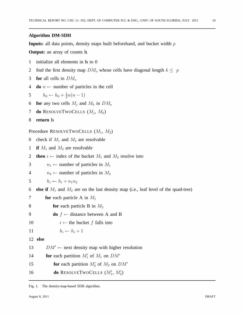
The pseudocode of the DM-SDH algorithm can be found in Fig. 1.The core of the algorithm
is a procedure named RESOLVETWOCELLS, which is given as inputs a pair of cellsM1 and
M2 on the same density map. In RESOLVETWOCELLS, we first compute the minimum and
maximum distances between any particle fromM1 and any one fromM2 (line 1). Obviously,
this can be accomplished in constant time given the corner coordinates of two cells stored in
the density map. When the minimum and maximum distances betweenM1 andM2 fall into the
same histogram bucketi, we say these two cells areresolvableon this density map, and they
resolveinto bucketi. If this happens, the histogram is updated (lines 2 - 5) by incrementing the
count of the specific bucketi by n1n2 wheren1, n2 are the particle counts in cellsM1 andM2,
respectively. If the two cells do not resolve on the current density map, we move to a density
map with higher (doubled) resolution and repeat the previous step. However, on this new density
map, we try resolving all four partitions ofM1 with all those ofM2 (lines 12 - 16). In other
words, there are4 × 4 = 16 recursive calls to RESOLVETWOCELLS if M1 and M2 are not
resolvable on the current density map. In another scenario whereM1 andM2 are not resolvable
yet no more density maps are available, we have to calculate the distances of all particles in the
non-resolvable cells (lines 6 - 11). The DM-SDH algorithm starts at the first density mapDMo
whose cell diagonal length is smaller than the histogram bucket width p (line 2). It is easy to
August 8, 2011 DRAFT
TECHNICAL REPORT NO. CSE/ 11- 052, DEPT. OF COMPUTER SCI. & ENG., UNIV. OF SOUTH FLORIDA, JULY 2011 10
Algorithm DM-SDH
Inputs: all data points, density maps built beforehand, and bucket width p
Output: an array of countsh
1 initialize all elements inh to 0
2 find the first density mapDMo whose cells have diagonal lengthk ≤ p
3 for all cells in DMo
4 do n← number of particles in the cell
5 h0 ← h0 + 12n(n− 1)
6 for any two cellsMj andMk in DMo
7 do RESOLVETWOCELLS (Mj , Mk)
8 return h
Procedure RESOLVETWOCELLS (M1, M2)
0 check ifM1 andM2 are resolvable
1 if M1 andM2 are resolvable
2 then i← index of the bucketM1 andM2 resolve into
3 n1 ← number of particles inM1
4 n2 ← number of particles inM2
5 hi ← hi + n1n2
6 else if M1 andM2 are on the last density map (i.e., leaf level of the quad-tree)
7 for each particle A inM1
8 for each particle B inM2
9 do f ← distance between A and B
10 i← the bucketf falls into
11 hi ← hi + 1
12 else
13 DM ′ ← next density map with higher resolution
14 for each partitionM ′1 of M1 on DM ′
15 for each partitionM ′2 of M2 on DM ′
16 do RESOLVETWOCELLS (M ′1, M ′
2)
Fig. 1. The density-map-based SDH algorithm.
August 8, 2011 DRAFT
TECHNICAL REPORT NO. CSE/ 11- 052, DEPT. OF COMPUTER SCI. & ENG., UNIV. OF SOUTH FLORIDA, JULY 2011 11
see that no pairs of cells are resolvable in density maps withresolution lower than that ofDMo.
Within each cell onDMo, we are sure that any intra-cell point-to-point distance issmaller than
p thus all such distances are counted into the first bucket withrange[0, p) (lines 3 - 5). The
algorithm proceeds by resolving inter-cell distances (i.e., calling RESOLVETWOCELLS) for all
pairs of cells inDMo (lines 6 - 7).
Clearly, by only considering atom counts in the density map cells (i.e., quad tree nodes),
we are able to process multiple point-to-point distances between two cells in one shot. This
translates into significant performance improvements overthe brute-force approach.
In DM-SDH, we assume there are a series of density maps built beforehand in the form of
a quad-tree. An important implementation detail that is relevant to our approximate algorithm
design is the height of the quad tree (i.e., the number of density map levels). Recall that DM-SDH
saves time by resolving cells such that we need not to calculate the point-to-point distances one
by one. However, when the total point counts in a cell decreases, the time we save by resolving
that cell also decreases. Imagine a cell with only 4 or fewer (8 for 3D data/space) data points,
it does not give us any benefit in processing SDH to further partition this cell on the next level:
the cost of resolving the partitions could be higher than directly retrieving the particles and
calculating distances (lines 7 - 11 in RESOLVETWOCELLS). Based on this observation, the total
level of density mapsH is set to be
H =
⌈
log2d
N
β
⌉
+ 1 (2)
whered is the number of dimensions,2d is the degree of the nodes in the tree (4/8 for 2D/3D
data) andβ is the average number of particles we desire in each leaf node. In practice, we set
β to be slightly greater than 4 in 2D (8 for 3D data) since the CPUcost of resolving two cells
is higher than computing the distance between two points.
B. Performance Analysis ofDM-SDH
We have accomplished a rigorous analysis of the performanceof DM-SDH and derived its
time complexity. The analysis focuses on the quantity of number of point-to-point distances
that can be covered in resolved cells. We generate closed-form formulae for such quantities
via a geometric modeling approach therefore rigorous analysis of the time complexity becomes
possible. While the technical details of the analytical model are complex and can be found in a
August 8, 2011 DRAFT
TECHNICAL REPORT NO. CSE/ 11- 052, DEPT. OF COMPUTER SCI. & ENG., UNIV. OF SOUTH FLORIDA, JULY 2011 12
recent article [27], it is necessary to sketch the most important (and also most relevant) analytical
results here for the purpose of laying out a foundation for the proposed approximate algorithm.
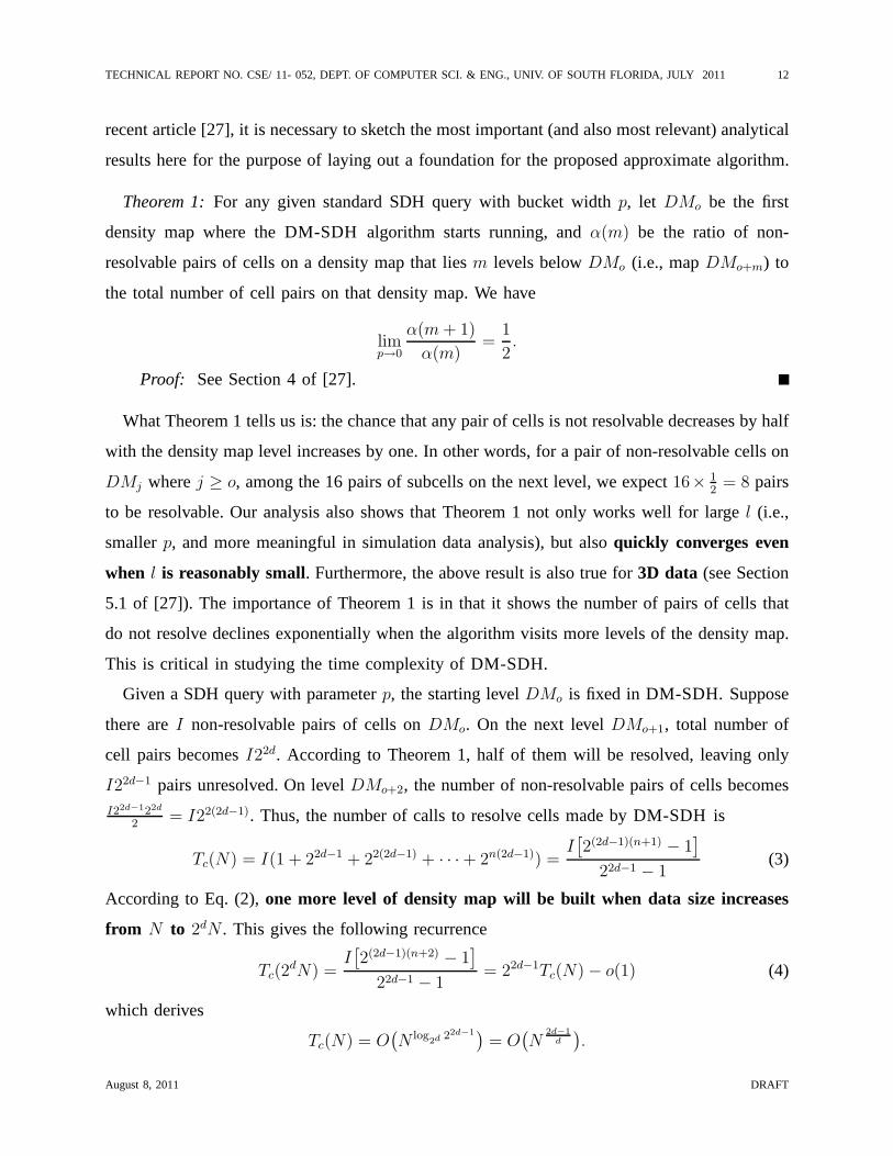
Theorem 1:For any given standard SDH query with bucket widthp, let DMo be the first
density map where the DM-SDH algorithm starts running, andα(m) be the ratio of non-
resolvable pairs of cells on a density map that liesm levels belowDMo (i.e., mapDMo+m) to
the total number of cell pairs on that density map. We have
limp→0
α(m + 1)
α(m)=
1
2.
Proof: See Section 4 of [27].
What Theorem 1 tells us is: the chance that any pair of cells isnot resolvable decreases by half
with the density map level increases by one. In other words, for a pair of non-resolvable cells on
DMj wherej ≥ o, among the 16 pairs of subcells on the next level, we expect16× 12
= 8 pairs
to be resolvable. Our analysis also shows that Theorem 1 not only works well for largel (i.e.,
smallerp, and more meaningful in simulation data analysis), but alsoquickly converges even
when l is reasonably small. Furthermore, the above result is also true for3D data (see Section
5.1 of [27]). The importance of Theorem 1 is in that it shows the number of pairs of cells that
do not resolve declines exponentially when the algorithm visits more levels of the density map.
This is critical in studying the time complexity of DM-SDH.
Given a SDH query with parameterp, the starting levelDMo is fixed in DM-SDH. Suppose
there areI non-resolvable pairs of cells onDMo. On the next levelDMo+1, total number of
cell pairs becomesI22d. According to Theorem 1, half of them will be resolved, leaving only
I22d−1 pairs unresolved. On levelDMo+2, the number of non-resolvable pairs of cells becomesI22d−122d
2= I22(2d−1). Thus, the number of calls to resolve cells made by DM-SDH is
Tc(N) = I(1 + 22d−1 + 22(2d−1) + · · ·+ 2n(2d−1)) =I[
2(2d−1)(n+1) − 1]
22d−1 − 1(3)
According to Eq. (2),one more level of density map will be built when data size increases
from N to 2dN . This gives the following recurrence
Tc(2dN) =
I[
2(2d−1)(n+2) − 1]
22d−1 − 1= 22d−1Tc(N)− o(1) (4)
which derives
Tc(N) = O(
N log2d 22d−1)
= O(
N2d−1
d
)
.
August 8, 2011 DRAFT
TECHNICAL REPORT NO. CSE/ 11- 052, DEPT. OF COMPUTER SCI. & ENG., UNIV. OF SOUTH FLORIDA, JULY 2011 13
Given Theorem 1, it is easy to find that the number of distancesin the non-resolvable cells also
follows the same recurrence as shown in Eq. (4) (see Section 6of [27]). By that, we conclude
the time complexity of the DM-SDH algorithm isO(
N2d−1
d
)
.
IV. THE APPROXIMATE DENSITY MAP-BASED SDH ALGORITHM
In this section, we introduce a modified SDH algorithm to givesuch approximate results to
gain better performance in return. Our solution targets at two must-have features of a decent
approximate algorithm :1) provable and controllable errorbounds such that the users can have
an idea on how close the results are to the fact; and 2) analysis of costs to reach (below) a given
error bound, which guides desired performance/correctness tradeoffs.
In the DM-SDH algorithm, we have to : 1) keep resolving cells till we reach the lowest
level of the tree; 2) calculate point-to-point distances when we cannot resolve two cells on
the leaf level of the tree. Our idea for approximate SDH processing is:stop at a certain tree
level and totally skip all distance calculations if we are sure that the number of distances in
the unvisited cell pairs fall below some error tolerance threshold. We name the new algorithm
as ADM-SDH (that stands for Approximate Density Map-based SDH), and it can be easily
implemented by modifying the DM-SDH algorithm. In particular, we stop the recursive calls
to RESOLVETWOCELLS after m levels. The critical problem, however, is how to determine the
value of m given a user-specified error tolerance boundǫ. In this paper, we use the following
metric to quantify the errors
e =
∑
i |hi − h′i|
∑
i hi
where for any bucketi, hi is the accurate count andh′i the count given by the approximate
algorithm.
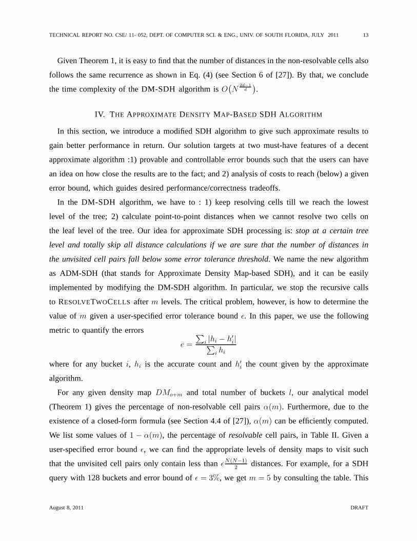
For any given density mapDMo+m and total number of bucketsl, our analytical model
(Theorem 1) gives the percentage of non-resolvable cell pairs α(m). Furthermore, due to the
existence of a closed-form formula (see Section 4.4 of [27]), α(m) can be efficiently computed.
We list some values of1 − α(m), the percentage ofresolvablecell pairs, in Table II. Given a
user-specified error boundǫ, we can find the appropriate levels of density maps to visit such
that the unvisited cell pairs only contain less thanǫN(N−1)2
distances. For example, for a SDH
query with 128 buckets and error bound ofǫ = 3%, we getm = 5 by consulting the table. This
August 8, 2011 DRAFT

TECHNICAL REPORT NO. CSE/ 11- 052, DEPT. OF COMPUTER SCI. & ENG., UNIV. OF SOUTH FLORIDA, JULY 2011 14
TABLE II
EXPECTED PERCENTAGE OF PAIRS OF CELLS THAT CAN BE RESOLVED UNDER DIFFERENT LEVELS OF DENSITY MAPS AND
TOTAL NUMBER OF HISTOGRAM BUCKETS. COMPUTED WITH MATHEMATICA 6.0.
Map Total Number of Buckets
levels 2 8 32 128 256
1 50.6565 52.5131 52.6167 52.6225 52.6227
2 74.8985 76.2390 76.3078 76.3112 76.3114
3 87.3542 88.1171 88.1539 88.1556 88.1557
4 93.6550 94.0582 94.0777 94.0778 94.0778
5 96.8222 97.0290 97.0285 97.0389 97.0389
6 98.4098 98.5145 98.5198 98.5195 98.5195
7 99.2046 99.2572 99.2596 99.2597 99.2597
8 99.6022 99.6286 99.6298 99.6299 99.6299
9 99.8011 99.8143 99.8149 99.8149 99.8149
10 99.9005 99.9072 99.9075 99.9075 99.9075
means, to ensure the 3% error bound, we only need to visit five levels of the tree (excluding
the starting levelDMo), and no distance calculation is needed. Table II serves as an excellent
validation of Theorem 1:α(m) almost exactly halves itself whenm increases by 1, even when
l is as small as 2. Since the numbers on the first row (i.e., values for 1 − α(1)) are also close
to 0.5, the correct choice ofm for the guaranteed error rateǫ is
m = lg1
ǫ.
The cost of the approximate algorithm only involves resolving cells on them + 1 levels of
density maps. From formula (4), we obtain the time complexity of the new algorithm
Tc(N) ≈ I2(2d−1)m = I2(2d−1) lg 1ǫ = I
(
1
ǫ
)2d−1
(5)
whereI is the number of cell pairs on the starting density mapDMo, and it is solely determined
by the query parameterp. Apparently, the running time of this algorithm is not related to the
input sizeN .
A. Heuristic Distribution of Distance Counts
August 8, 2011 DRAFT

TECHNICAL REPORT NO. CSE/ 11- 052, DEPT. OF COMPUTER SCI. & ENG., UNIV. OF SOUTH FLORIDA, JULY 2011 15
(i-1)p ip (i+1)p (i+2)pu v......
distance
Range of inter-cell
distances
bucket
i+1
bucket
i
bucket
i+2
Fig. 2. Distance range of two resolvable cells overlap with three
buckets.
Now let us discuss how to deal with
those non-resolvable cells after visiting
m + 1 levels on the tree. In giving the
error bounds in our approximate algo-
rithm, we are conservative in assuming
the distances in all the unresolved cells will be placed intothe wrong bucket. In fact, this almost
will never happen because we can distribute the distance counts in the unvisited cells to the
histogram buckets heuristically and some of them will be done correctly. Consider two non-
resolvable cells in a density map with particle countsn1 and n2 (i.e., total number ofn1n2
distances between them), respectively. We know their minimum and maximum distancesu and
v (these are calculated beforehand in our attempt to resolve them) fall into multiple buckets. Fig.
2 shows an example that spans three buckets. Using this example, we describe the following
heuristics to distribute then1n2 total distance counts into the relevant buckets. These heuristics
are ordered in their expected correctness.
1. Put alln1n2 distance counts into one bucket that is predetermined (e.g., always putting the
counts to the leftmost bucket); We name this heuristic as SKEW;
2. Evenly distribute the distance counts into the three buckets that[u, v] overlaps, i.e., each
bucket gets13n1n2; this heuristic is named EVEN;
3. Distribute the distance counts based on the overlaps between range[u, v] and the buckets.
In Fig. 2, the distances put into bucketsi, i + 1, and i + 2 are n1n2ip− u
v − u, n1n2
p
v − r,
andn1n2v − (i + 1)p
v − u, respectively. Apparently, by adapting this approach, we assume the
(statistical) distribution of the point-to-point distances between the two cells is uniform.
This heuristic is called PROP (short forproportional).
The assumption of uniform distance distribution in PROP is obviously an oversimplification.
In [29], we briefly mentioned a 4th heuristic: if we know the spatial distribution of particles within
individual cells, we can generate the statistical distribution of the distances either analytically or
via simulations, and put then1n2 distances to involved buckets based on this distribution. This
solution involves very non-trivial statistical inferenceof the particle spatial distribution and is
beyond the scope of this paper.
August 8, 2011 DRAFT

TECHNICAL REPORT NO. CSE/ 11- 052, DEPT. OF COMPUTER SCI. & ENG., UNIV. OF SOUTH FLORIDA, JULY 2011 16
Note that all above methods require only constant time to compute a solution for two cells.
Therefore, the time complexity of ADM-SDH is not affected nomatter which heuristic is used.
V. EMPIRICAL EVALUATION OF ADM-SDH
Fig. 3. The simulated hydrated dipalmi-
toylphosphatidylcholine bilayer system. We
can see two layers of hydrophilic head groups
(with higher atom density) connected to hy-
drophobic tails (lower atom density) are sur-
rounded by water molecules (red dots).
We have implemented the ADM-SDH algorithm using
the C programming language and tested it with various
synthetic/real datasets. The experiments are run at an Apple
Mac Pro workstation with two dual-core 2.66GHz Intel Xeon
CPUs, and 8GB of physical memory. The operating system
is OS X 10.5 Leopard. In these experiments, we set the
program to stop after visiting different levels of density
maps and distribute the distances using the three heuristics
(Section IV). We then compare the approximate histogram
with those generated by regular DM-SDH. We use various
synthetic and real data sets in our experiments. The synthetic
data are generated from: (1) uniform distributions to simulate
a system with particles evenly distributed in space; and (2)
Zipf distribution with order 1 to introduce skewness to data
spatial distribution. The real datasets are extracted froma
molecular simulation of biomembrane structures (Fig. 3). The data size in such experiments
range from 50,000 to 12,800,000.
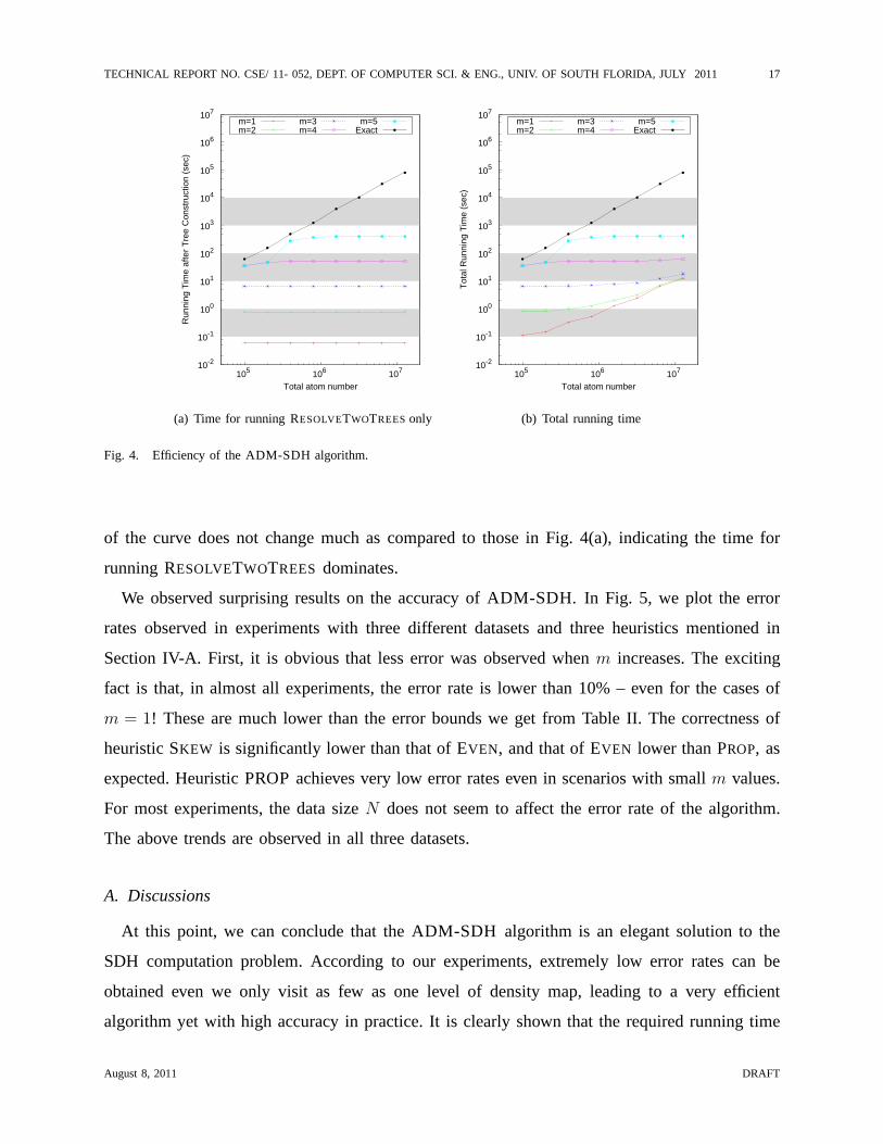
Fig. 4 shows the running time of ADM-SDH under one singlep value of 2500.0. Note that
the ‘Exact’ line shows the results of the basic DM-SDH algorithm whose running time obviously
increases polynomially withN at a slope of about 1.5. First, we can easily conclude that the
running time after the tree construction stage does not change with the increase of dataset size
(Fig. 4(a)). The only exception is whenm is 5 – the running time increases whenN is small and
then stays as a constant afterwards. This is because the algorithm has less than 5 levels to visit
in a bushy tree resulted from smallN values. WhenN is large enough, running time no longer
changes with the increase ofN . In Fig. 4(b), we plot the total running time which includes the
time for quad-tree construction. Under smallm values, the tree construction time is a dominating
factor since it increases with data sizeN (i.e., O(N log N)). However, whenm > 3, the shape
August 8, 2011 DRAFT
TECHNICAL REPORT NO. CSE/ 11- 052, DEPT. OF COMPUTER SCI. & ENG., UNIV. OF SOUTH FLORIDA, JULY 2011 17
10-2
10-1
100
101
102
103
104
105
106
107
105 106 107
Run
ning
Tim
e af
ter
Tre
e C
onst
ruct
ion
(sec
)
Total atom number
m=1m=2
m=3m=4
m=5Exact
(a) Time for running RESOLVETWOTREESonly
10-2
10-1
100
101
102
103
104
105
106
107
105 106 107
Tot
al R
unni
ng T
ime
(sec
)
Total atom number
m=1m=2
m=3m=4
m=5Exact
(b) Total running time
Fig. 4. Efficiency of the ADM-SDH algorithm.
of the curve does not change much as compared to those in Fig. 4(a), indicating the time for
running RESOLVETWOTREES dominates.
We observed surprising results on the accuracy of ADM-SDH. In Fig. 5, we plot the error
rates observed in experiments with three different datasets and three heuristics mentioned in
Section IV-A. First, it is obvious that less error was observed whenm increases. The exciting
fact is that, in almost all experiments, the error rate is lower than 10% – even for the cases of
m = 1! These are much lower than the error bounds we get from Table II. The correctness of
heuristic SKEW is significantly lower than that of EVEN, and that of EVEN lower than PROP, as
expected. Heuristic PROP achieves very low error rates evenin scenarios with smallm values.
For most experiments, the data sizeN does not seem to affect the error rate of the algorithm.
The above trends are observed in all three datasets.
A. Discussions
At this point, we can conclude that the ADM-SDH algorithm is an elegant solution to the
SDH computation problem. According to our experiments, extremely low error rates can be
obtained even we only visit as few as one level of density map,leading to a very efficient
algorithm yet with high accuracy in practice. It is clearly shown that the required running time
August 8, 2011 DRAFT

TECHNICAL REPORT NO. CSE/ 11- 052, DEPT. OF COMPUTER SCI. & ENG., UNIV. OF SOUTH FLORIDA, JULY 2011 18
10-5
10-4
10-3
10-2
10-1
100
Err
or r
ate
SKEW
EVEN
PROP
m=1 m=2 m=3
m=4m=5
10-5
10-4
10-3
10-2
10-1
100
Err
or r
ate
10-5
10-4
10-3
10-2
10-1
100
105 106 107
Err
or r
ate
Number of atoms
105 106 107
Number of atoms
105 106 107
Number of atoms
Uni
form
Dat
aZ
ipf D
ata
Rea
l Dat
a
Fig. 5. Accuracy of the ADM-SDH algorithm.
for ADM-SDH grows nicely with the data sizeN (i.e., only whenm is of a small value does
the tree construction time dominate).
The errors rates achieved by ADM-SDH approximate algorithmshown by current experiments
are much lower than what we expected from our basic analysis.For example, Table II predicts
an error rate of around 48% for the case ofm = 1, yet the error we observed form = 1 in
our experiments is no more than 10%. With the PROP heuristic, this value can be as low as
0.5%. Our explanation for such low error rates is: in an individual operation to distribute the
distance counts heuristically, we could have rendered a large error by putting too many counts
into a bucket (e.g., bucketi in Fig. 2) than needed. But the effects of this mistake could be
August 8, 2011 DRAFT
TECHNICAL REPORT NO. CSE/ 11- 052, DEPT. OF COMPUTER SCI. & ENG., UNIV. OF SOUTH FLORIDA, JULY 2011 19
(partially) canceled out by another distribution operation, in which too few counts are put into
bucket i. Note that the total error in a bucket is calculated after alloperations are processed,
thus it reflects the net effects of all positive and negative errors from individual operations. We
call this phenomenonerror compensation.
While more experiments under different scenarios are obviously needed, investigations from
an analytical viewpoint are necessary. From the above facts, we understand that the bound given
by Table II is loose. The real error bound should be describedas
ǫ = ǫ′
ǫ′′
(6)
whereǫ′
is the percentage of resolved distances given by Table II andǫ′′
is the error rate created
by the heuristics via error compensation. In the following section, we develop an analytical model
to study how error compensation dramatically boosts accuracy of the algorithm.
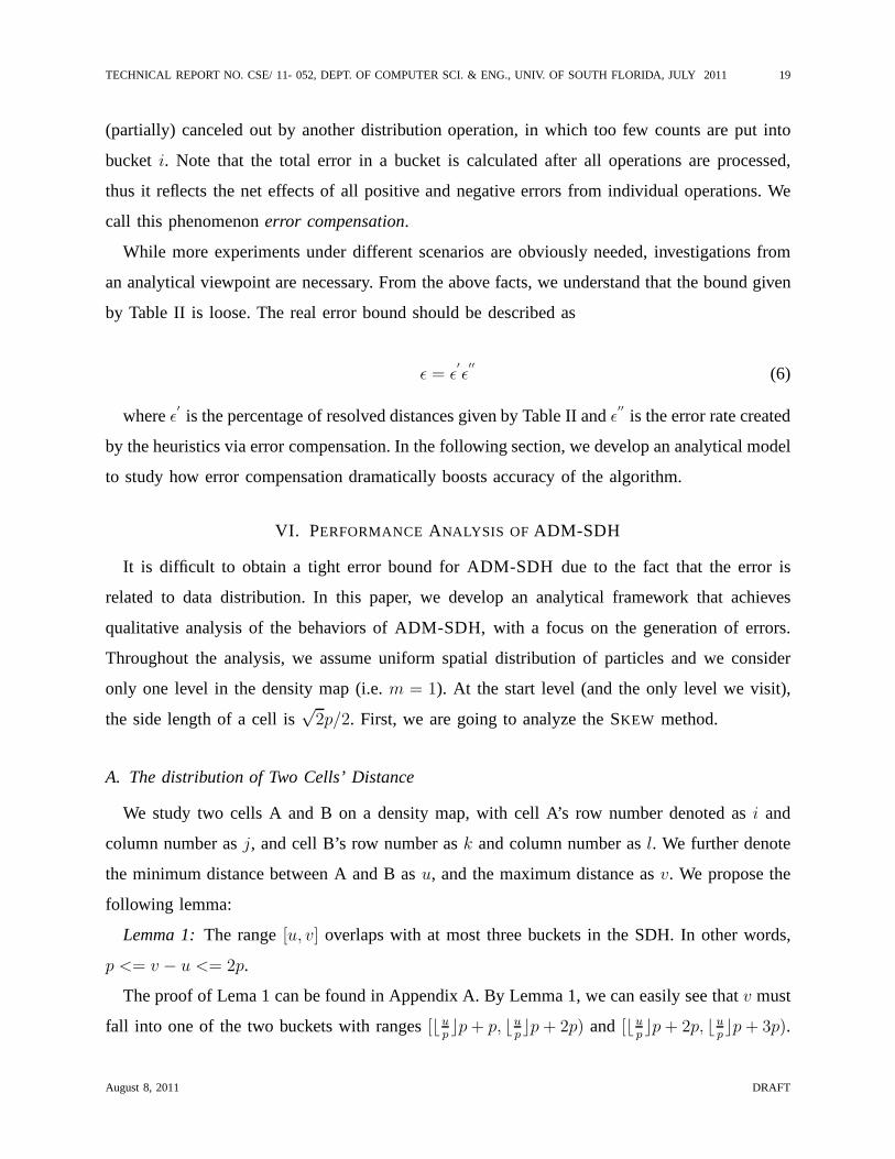
VI. PERFORMANCE ANALYSIS OF ADM-SDH
It is difficult to obtain a tight error bound for ADM-SDH due tothe fact that the error is
related to data distribution. In this paper, we develop an analytical framework that achieves
qualitative analysis of the behaviors of ADM-SDH, with a focus on the generation of errors.
Throughout the analysis, we assume uniform spatial distribution of particles and we consider
only one level in the density map (i.e.m = 1). At the start level (and the only level we visit),
the side length of a cell is√
2p/2. First, we are going to analyze the SKEW method.
A. The distribution of Two Cells’ Distance
We study two cells A and B on a density map, with cell A’s row number denoted asi and
column number asj, and cell B’s row number ask and column number asl. We further denote
the minimum distance between A and B asu, and the maximum distance asv. We propose the
following lemma:
Lemma 1:The range[u, v] overlaps with at most three buckets in the SDH. In other words,
p <= v − u <= 2p.
The proof of Lema 1 can be found in Appendix A. By Lemma 1, we caneasily see thatv must
fall into one of the two buckets with ranges[⌊up⌋p + p, ⌊u
p⌋p + 2p) and [⌊u
p⌋p + 2p, ⌊u
p⌋p + 3p).
August 8, 2011 DRAFT
TECHNICAL REPORT NO. CSE/ 11- 052, DEPT. OF COMPUTER SCI. & ENG., UNIV. OF SOUTH FLORIDA, JULY 2011 20
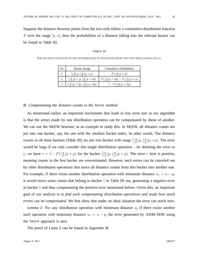
Suppose the distance between points from the two cells follow a cumulative distribution function
F over the range[u, v], then the probabilities of a distance falling into the relevant bucket can
be found in Table III.
TABLE III
THE BUCKETS INVOLVED IN THE DISTRIBUTION OF DISTANCES FROM TWO NON-RESOLVABLE CELLS.
No Bucket Range Cumulative Probabilities
1 [⌊u
p⌋p, ⌊u
p⌋p + p) F (⌊u
p⌋p + p)
2 [⌊u
p⌋p + p, ⌊u
p⌋p + 2p) F (⌊u
p⌋p + 2p) − F (⌊u
p⌋p + p)
3 [⌊u
p⌋p + 2p, ⌊u
p⌋p + 3p) 1 − F (⌊u
p⌋p + 2p)
B. Compensating the distance counts in theSKEW method
As mentioned earlier, an important mechanism that leads to low error rate in our algorithm
is that the errors made by one distribution operation can be compensated by those of another.
We can use the SKEW heuristic as an example to study this. In SKEW, all distance counts are
put into one bucket, say, the one with the smallest bucket index. In other words, The distance
counts in all three buckets (Table III) are put into bucket with range[⌊up⌋p, ⌊u
p⌋p+ p). The error
would be large if we only consider this single distribution operation – by denoting the error as
e, we havee = 1− F (⌊up⌋p + p) for the bucket[⌊u
p⌋p, ⌊u
p⌋p + p). The errore here is positive,
meaning counts in the first bucket are overestimated. However, such errors can be canceled out
by other distribution operations that move all distance counts from this bucket into another one.
For example, if there exists another distribution operation with minimum distanceu1 = u − p,
it would move some counts that belong to bucket1 in Table III out, generating a negative error
in bucket1 and thus compensating the positive error mentioned before.Given this, an important
goal of our analysis is tofind such compensating distribution operations and study how much
errors can be compensated. We first show that under an ideal situation the error can reach zero.
Lemma 2:For any distribution operation with minimum distanceu, if there exists another
such operation with minimum distanceu1 = u − p, the error generated by ADM-SDH using
the SKEW approach is zero.
The proof of Lema 2 can be found in Appendix B.
August 8, 2011 DRAFT
TECHNICAL REPORT NO. CSE/ 11- 052, DEPT. OF COMPUTER SCI. & ENG., UNIV. OF SOUTH FLORIDA, JULY 2011 21
In the following text, we study how the errors can be partially compensated by neighboring
pairs of cells.
u
u1
B
B
r
r1
A
C
C
Fig. 6. Pairs of cells that lead to par-
tial error compensation in the SKEW
approach.
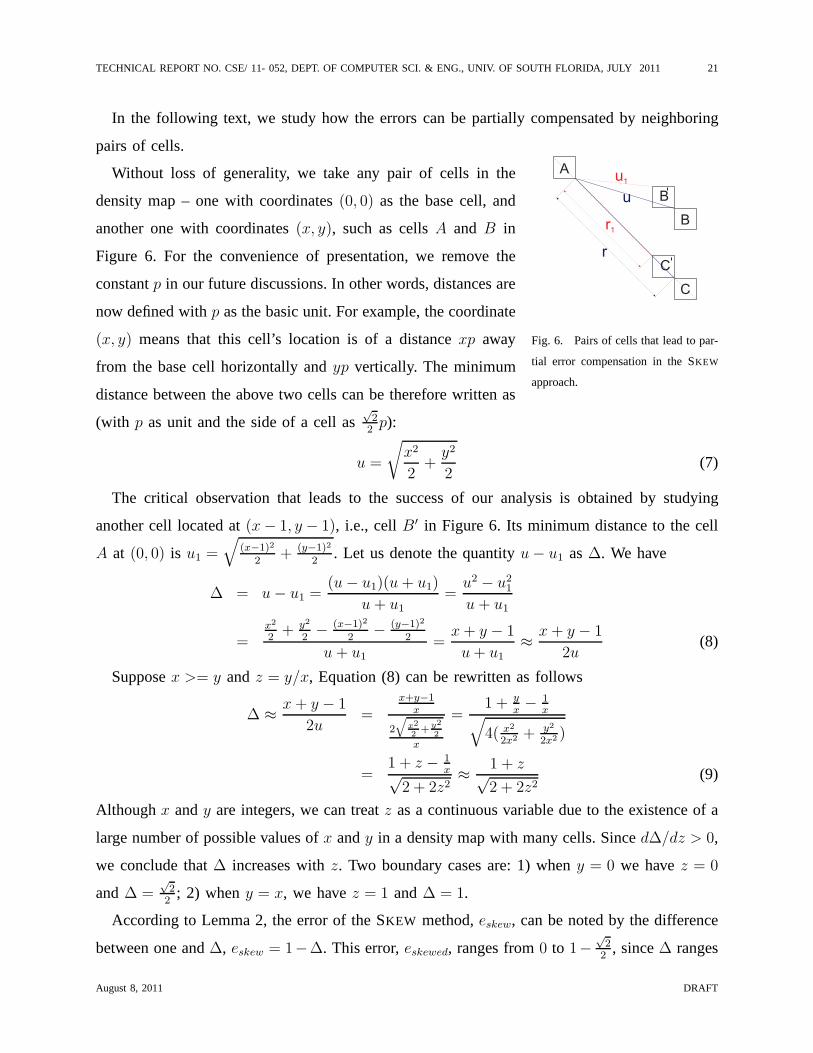
Without loss of generality, we take any pair of cells in the
density map – one with coordinates(0, 0) as the base cell, and
another one with coordinates(x, y), such as cellsA and B in
Figure 6. For the convenience of presentation, we remove the
constantp in our future discussions. In other words, distances are
now defined withp as the basic unit. For example, the coordinate
(x, y) means that this cell’s location is of a distancexp away
from the base cell horizontally andyp vertically. The minimum
distance between the above two cells can be therefore written as
(with p as unit and the side of a cell as√
22
p):
u =
√
x2
2+
y2
2(7)
The critical observation that leads to the success of our analysis is obtained by studying
another cell located at(x− 1, y − 1), i.e., cellB′ in Figure 6. Its minimum distance to the cell
A at (0, 0) is u1 =√
(x−1)2
2+ (y−1)2
2. Let us denote the quantityu− u1 as∆. We have
∆ = u− u1 =(u− u1)(u + u1)
u + u1
=u2 − u2
1
u + u1
=x2
2+ y2
2− (x−1)2
2− (y−1)2
2
u + u1=
x + y − 1
u + u1≈ x + y − 1
2u(8)
Supposex >= y andz = y/x, Equation (8) can be rewritten as follows
∆ ≈ x + y − 1
2u=
x+y−1x
2
q
x2
2+ y2
2
x
=1 + y
x− 1
x√
4( x2
2x2 + y2
2x2 )
=1 + z − 1
x√2 + 2z2
≈ 1 + z√2 + 2z2
(9)
Althoughx andy are integers, we can treatz as a continuous variable due to the existence of a
large number of possible values ofx andy in a density map with many cells. Sinced∆/dz > 0,
we conclude that∆ increases withz. Two boundary cases are: 1) wheny = 0 we havez = 0
and∆ =√
22
; 2) wheny = x, we havez = 1 and∆ = 1.
According to Lemma 2, the error of the SKEW method,eskew, can be noted by the difference
between one and∆, eskew = 1−∆. This error,eskewed, ranges from0 to 1−√
22
, since∆ ranges
August 8, 2011 DRAFT

TECHNICAL REPORT NO. CSE/ 11- 052, DEPT. OF COMPUTER SCI. & ENG., UNIV. OF SOUTH FLORIDA, JULY 2011 22
from√
22
to 1. The compensating process in distance counts is shown in Figure 6. As mentioned
before,C andC ′ are examples of two cells for which the difference of minimumdistances to
cell A is 1 and the cellsB andB′ are two cells for which the difference of minimum distances
is different from one (less than one in this case).
A
B
D
C E T
U
F
D
S
S
G H H I
W
u-1 uu1
Fig. 7. Compensating the distance counts
Figure 7 represents the triangular density dis-
tributions of three different minimum distances,
u, u1 and u − 1. In our analysis we have used
normal distribution in stead of triangular, based
on the approximation shown in appendix C.u is
the minimum distance between the base cell and
the cell which is located at(x, y) and u1 is the
minimum distance between the base cell and the cell which is located at(x− 1, y − 1). In our
analysis we defineG as ⌊u⌋, and we also defineH = G + 1 and I = H + 1. The triangles of
STU , AEW andBCF are the density distributions of the minimum distancesu, u1 andu− 1,
respectively. The lineH ′S ′D′ is the symmetry line ofWFH with respect to the vertical line
which passes through the point D.
As we know, if u1 = u − 1, the error of distance counts produced by the period betweenH
and I can be compensated by that produced by the period betweenG andH. In other words,
according to SKEW, when we count the number of distances between the cell at coordinates
(0, 0) and the cell located at(x, y), the number of distances betweenH and I is added and
leads to a positive error. When we count the number of distances between the base cell and the
cell which is located at(x− 1, y− 1), the number of distances betweenG andH is missed and
leads to a negative error. If the distribution is the same, the area ofGBCFH is the same as the
area ofHSTUI.
0.1
0.2
0.3
0.4
0.1 0.2 0.3 0.4 0.5 0.6 0.7 0.8 0.9 1 X
Y
0.211*(1-z) +0.211*(1-z)5 22+2z
2
1+z- 1
Fig. 8. Approximation of 1∆
− 1
If u1 6= u − 1, there is difference be-
tween the area ofGAEWH and the area of
HSTUI. In other words, there is difference
between the area ofGAEWH and the area of
GBCFH. This difference can be computed
by the area ofABD′S ′ and that represents
the error imposed by the difference between
August 8, 2011 DRAFT

TECHNICAL REPORT NO. CSE/ 11- 052, DEPT. OF COMPUTER SCI. & ENG., UNIV. OF SOUTH FLORIDA, JULY 2011 23
u1 andu− 1 which we denote aseu1,u−1. We
know that CE = u1 − u + 1 and GH ′ <
u − u1 = ∆. Considering the fact that the
area of each of the three triangles in Figure 7
is one, the height of each of these triangles is2v−u
(since the base isv−u). Therefore, the ratioABCE
has the following value (for more detailed explanation, please refer to Appendix D):
AB
CE=
2v−uv−u
2
=4
(v − u)2(10)
Furthermore, the length ofAB is:
AB =4
(v − u)2∗ CE =
4(u1 − u + 1)
(v − u)2=
4(1−∆)
(v − u)2(11)
The area ofABD′S ′, thus the erroreu1,u−1, can be computed as follows:
eu1,u−1 = AB ∗GH ′ <4(1−∆) ∗∆
(v − u)2(12)
eu1,u−1 <(1−∆)
∆=
1
∆− 1 (13)
Therefore the accumulated error,ez=0,1 over the range ofz, z = 0, 1 can be computed by the
following equation (considering Eq. (9) for∆)
ez=0,1 =
1∑
z=0
eu1,u−1 =
1∑
z=0
(1
∆− 1) ≈
1∑
z=0
(
√2 + 2z2
1 + z− 1
)
(14)
When0 ≤ z ≤ 1, we can approximateez=0,1 as follows (from Figure 8).
ez=0,1 ≤1
∑
z=0
0.211 ∗ (1− z)5 + 0.211 ∗ (1− z)2 (15)
ez=0,1 =
∫ 1
0
(0.211 ∗ (1− z)5 + 0.211 ∗ (1− z)2) dz = 0.1055 (16)
Eq. (16) means that the total error rendered by the SKEW under the assumptions we stated
in the beginning of Section VI is less than 10.55%. Due to the assumptions we made, we do
not claim this as a rigorous bound. However, it clearly showsthat our algorithm is able to
produce really good results with low errors by visiting onlyone level in the density map. And
this conclusion builds the foundation of an improved approximate algorithm (Section VII).
August 8, 2011 DRAFT

TECHNICAL REPORT NO. CSE/ 11- 052, DEPT. OF COMPUTER SCI. & ENG., UNIV. OF SOUTH FLORIDA, JULY 2011 24
One special note here is that Eq. (16) does not cover the casesin which the minimum distance
u falls into the first SDH bucket (i.e.,u < p). However, our analysis shows that such cases do
not impact the results in Eq. (16) significantly. More details can be found in Appendix E.
VII. SINGLE LEVEL APPROXIMATE ALGORITHM
Via the performance analysis of ADM-SDH, and looking back tothe error bound described
in Eq. (6), we concluded thatǫ′′ is very small. Even if we allowǫ′ be 100%, meaning no
cell resolution is needed, we can still achieve low and controllable error rates in our results.
Therefore, in this section, we introduce an improved approximate algorithm, we callsingle
level approximate algorithm(SL-SDH), based on such a conclusion. SL-SDH has all the same
parts as the original ADM-SDH algorithm with the only difference is that we nowvisit only one
density map (i.e., one level of the tree) instead of visitingm levels as in the original approximate
algorithm. SL-SDH improves over ADM-SDH in two important aspects. First, we only need a
singleDM which can be built inO(N) time (instead of theO(N log N) time needed to build
the quad tree). Second, we reduce the post-tree-construction running time of the algorithm, with
little increase of the error, as we only run RESOLVETWOTREES for cells in one density map.
However, the running time of SL-SDH still depends heavily onthe bucket widthp. Recall
that ADM-SDH starts at the density mapDM0 where the diagonal of a single cell is less than
or equal top. Whenp is small, the number of cells inDM0 is large, and we have to invoke the
RESOLVETWOCELLS procedure more times. To remedy this, we further modify SL-SDH by
allowing it to run on a (single) density map aboveDM0, i.e., one with larger cell sizes (and fewer
cells). This is based on a hypothesis motivated by our performance analysis of ADM-SDH: the
error compensation mechanism we studied will also work for density maps aboveDM0. We
know the error is very small for running, RESOLVETWOTREES for those cells inDM0 - doing
the same on higher level density maps should still render reasonable (although higher) error
rates. Unfortunately, an analytical study of such errors isvery difficult. In the remainder of this
section, we empirically evaluate the error and time tradeoff of the final version of the SL-SDH
algorithm.
August 8, 2011 DRAFT

TECHNICAL REPORT NO. CSE/ 11- 052, DEPT. OF COMPUTER SCI. & ENG., UNIV. OF SOUTH FLORIDA, JULY 2011 25
10-2
10-1
100
101
25 50 100 150 200 500 1000 1500 2000 2500 3000 3500 4000
Uniform Data7.5 Million atoms
Level 3
Level 4
Level 5
Level 6
Level 7
Level 8
Level 9
Bucket width
Error
in %
Real Data891,272 atoms
Level 3
Level 4
Level 5
Level 6
Level 7
Level 8
Level 9
Bucket width
Error
in %
Skewed Data
7.5 Million atoms
Level 3
Level 4
Level 5
Level 6
Level 7
Level 8
Level 9
Bucket width
Error
in %
10-2
10-1
100
101
10-2
10-1
100
101
102
25 50 100 150 200 500 1000 1500 2000 2500 3000 3500 4000
25 50 100 150 200 500 1000 1500 2000 2500 3000 3500 4000
Fig. 9. Accuracy of the SL-SDH algorithm under different bucket width for synthetic (uniform and skewed) and real data.
A. Experimental Results
We have implemented the SL-SDH algorithm using the C programming language and tested
it with various synthetic/real datasets. The experiments are run in the same environment as the
experiments for the ADM-SDH in Section V.
Since we know, from our previous experiments, that the PROP heuristic for distributing the
distances in non-resolvable cells produces the best results, we have only used that heuristic to
show the results of the single level approximate algorithm.We have run the algorithm on two
synthetic datasets, one with uniform and another with skewed distribution of atoms, under five
different numbers (i.e.,1, 3, 5, 7.5 and12 million) of atoms. We also ran the algorithm on one
real simulation dataset with891, 272 atoms. Figure 9 shows the results from the experiments on
uniform and skewed data respectively with7.5 million atoms and the real data with891, 272
August 8, 2011 DRAFT

TECHNICAL REPORT NO. CSE/ 11- 052, DEPT. OF COMPUTER SCI. & ENG., UNIV. OF SOUTH FLORIDA, JULY 2011 26
25 50 100 150 200 500 1000 1500 2000 2500 3000 3500 4000
Combined Uniform Data12 Million Atoms
Bucket width
Level 3
Level 4
Level 5Level 6
Level 7Level 8
Level 9
Error
in %
Combined Skewed Data12 Million Atoms
Bucket width
Level 3
Level 4
Level 5
Level 6Level 7
Level 8
Level 9
Error
in %
10-2
10-1
100
101
10-2
10-1
100
101
101
25 50 100 150 200 500 1000 1500 2000 2500 3000 3500 4000
Fig. 10. Accuracy of the SL-SDH algorithm under different bucket width and different atom counts for synthetic data (uniform
and skewed).
atoms. From these figures we can see that the error rate decreases when we increase the level
in the density map. We also see that the error rate is lower when the bucket width increases.
In Figure 10 we demonstrate the effects of system sizeN on the accuracy of SL-SDH. Each
line in Figure 10 plots the error rates of SL-SDH when run witha particular level of density
map under a particular atom count. We can easily see that the lines for the five different system
sizes (of the same density map) are very similar, giving riseto one cluster of lines for each level
of density map. The above two figures actually show that the error introduced by the SL-SDH
algorithm is not affected by the number of atoms in the dataset N , but by the level of density
map the algorithm works at. On the other hand, the running time of the SL-SDH algorithm was
also found to be independent ofN , as shown in Figure 11. The only exceptions are for levels
3 and 4, in which the tree construction time dominates.
The difference between SL-SDH and ADM-SDH can be seen by comparing Figure 11 with
Figure 4, and Figure 10 with Figure 5. However, to better understand the accuracy/performance
August 8, 2011 DRAFT
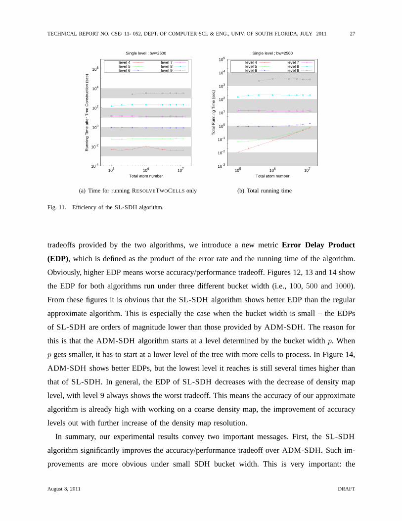
TECHNICAL REPORT NO. CSE/ 11- 052, DEPT. OF COMPUTER SCI. & ENG., UNIV. OF SOUTH FLORIDA, JULY 2011 27
10-4
10-2
100
102
104
106
105 106 107
Run
ning
Tim
e af
ter
Tre
e C
onst
ruct
ion
(sec
)
Total atom number
Single level ; bw=2500
level 4level 5level 6
level 7level 8level 9
(a) Time for running RESOLVETWOCELLS only
10-3
10-2
10-1
100
101
102
103
104
105
105 106 107
Tot
al R
unni
ng T
ime
(sec
)
Total atom number
Single level ; bw=2500
level 4level 5level 6
level 7level 8level 9
(b) Total running time
Fig. 11. Efficiency of the SL-SDH algorithm.
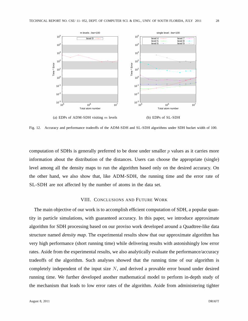
tradeoffs provided by the two algorithms, we introduce a newmetric Error Delay Product
(EDP), which is defined as the product of the error rate and the running time of the algorithm.
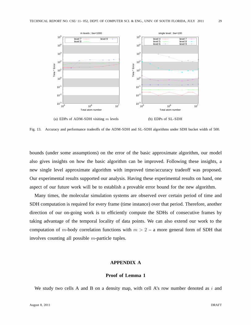
Obviously, higher EDP means worse accuracy/performance tradeoff. Figures 12, 13 and 14 show
the EDP for both algorithms run under three different bucketwidth (i.e., 100, 500 and 1000).
From these figures it is obvious that the SL-SDH algorithm shows better EDP than the regular
approximate algorithm. This is especially the case when thebucket width is small – the EDPs
of SL-SDH are orders of magnitude lower than those provided by ADM-SDH. The reason for
this is that the ADM-SDH algorithm starts at a level determined by the bucket widthp. When
p gets smaller, it has to start at a lower level of the tree with more cells to process. In Figure 14,
ADM-SDH shows better EDPs, but the lowest level it reaches isstill several times higher than
that of SL-SDH. In general, the EDP of SL-SDH decreases with the decrease of density map
level, with level 9 always shows the worst tradeoff. This means the accuracy of our approximate
algorithm is already high with working on a coarse density map, the improvement of accuracy
levels out with further increase of the density map resolution.
In summary, our experimental results convey two important messages. First, the SL-SDH
algorithm significantly improves the accuracy/performance tradeoff over ADM-SDH. Such im-
provements are more obvious under small SDH bucket width. This is very important: the
August 8, 2011 DRAFT
TECHNICAL REPORT NO. CSE/ 11- 052, DEPT. OF COMPUTER SCI. & ENG., UNIV. OF SOUTH FLORIDA, JULY 2011 28
10-3
10-2
10-1
100
101
102
103
104
105
105 106 107
Tim
e *
Err
or
Total atom number
m levels ; bw=100
level 9
(a) EDPs of ADM-SDH visitingm levels
10-3
10-2
10-1
100
101
102
103
104
105
105 106 107
Tim
e *
Err
or
Total atom number
single level ; bw=100
level 4level 5level 6
level 7level 8level 9
(b) EDPs of SL-SDH
Fig. 12. Accuracy and performance tradeoffs of the ADM-SDH and SL-SDH algorithms under SDH bucket width of 100.
computation of SDHs is generally preferred to be done under smallerp values as it carries more
information about the distribution of the distances. Userscan choose the appropriate (single)
level among all the density maps to run the algorithm based only on the desired accuracy. On
the other hand, we also show that, like ADM-SDH, the running time and the error rate of
SL-SDH are not affected by the number of atoms in the data set.
VIII. C ONCLUSIONS AND FUTURE WORK
The main objective of our work is to accomplish efficient computation of SDH, a popular quan-
tity in particle simulations, with guaranteed accuracy. Inthis paper, we introduce approximate
algorithm for SDH processing based on our proviso work developed around a Quadtree-like data
structure nameddensity map. The experimental results show that our approximate algorithm has
very high performance (short running time) while delivering results with astonishingly low error
rates. Aside from the experimental results, we also analytically evaluate the performance/accuracy
tradeoffs of the algorithm. Such analyses showed that the running time of our algorithm is
completely independent of the input sizeN , and derived a provable error bound under desired
running time. We further developed another mathematical model to perform in-depth study of
the mechanism that leads to low error rates of the algorithm.Aside from administering tighter
August 8, 2011 DRAFT
TECHNICAL REPORT NO. CSE/ 11- 052, DEPT. OF COMPUTER SCI. & ENG., UNIV. OF SOUTH FLORIDA, JULY 2011 29
10-3
10-2
10-1
100
101
102
103
104
105
105 106 107
Tim
e *
Err
or
Total atom number
m levels ; bw=1000
level 7level 8
level 9
(a) EDPs of ADM-SDH visitingm levels
10-3
10-2
10-1
100
101
102
103
104
105
105 106 107
Tim
e *
Err
or
Total atom number
single level ; bw=100
level 4level 5level 6
level 7level 8level 9
(b) EDPs of SL-SDH
Fig. 13. Accuracy and performance tradeoffs of the ADM-SDH and SL-SDH algorithms under SDH bucket width of 500.
bounds (under some assumptions) on the error of the basic approximate algorithm, our model
also gives insights on how the basic algorithm can be improved. Following these insights, a
new single level approximate algorithm with improved time/accuracy tradeoff was proposed.
Our experimental results supported our analysis. Having these experimental results on hand, one
aspect of our future work will be to establish a provable error bound for the new algorithm.
Many times, the molecular simulation systems are observed over certain period of time and
SDH computation is required for every frame (time instance)over that period. Therefore, another
direction of our on-going work is to efficiently compute the SDHs of consecutive frames by
taking advantage of the temporal locality of data points. Wecan also extend our work to the
computation ofm-body correlation functions withm > 2 – a more general form of SDH that
involves counting all possiblem-particle tuples.
APPENDIX A
Proof of Lemma 1
We study two cells A and B on a density map, with cell A’s row number denoted asi and
August 8, 2011 DRAFT

TECHNICAL REPORT NO. CSE/ 11- 052, DEPT. OF COMPUTER SCI. & ENG., UNIV. OF SOUTH FLORIDA, JULY 2011 30
10-3
10-2
10-1
100
101
102
103
104
105
105 106 107
Tim
e *
Err
or
Total atom number
m levels ; bw=1000
level 6level 7
level 8level 9
(a) EDPs of ADM-SDH visitingm levels
10-3
10-2
10-1
100
101
102
103
104
105
105 106 107
Tim
e *
Err
or
Total atom number
single level ; bw=1000
level 4level 5level 6
level 7level 8level 9
(b) EDPs of SL-SDH
Fig. 14. Accuracy and performance tradeoffs of the ADM-SDH and SL-SDH algorithms under SDH bucket width of 1000.
column number asj, and cell B’s row number ask and column number asl. We further denote
the minimum distance between A and B asu, and the maximum distance asv. Thenv andu
can be written as functions of the two cells’ row and column numbers as follows:
Case 1. When A and B are in different rows and columns, i.e.,i 6= k and j 6= l, we have
u = p
√
(i− k − 1)2
2+
(j − l − 1)2
2(17)
and
v = p
√
(i− k + 1)2
2+
(j − l + 1)2
2(18)
Case 2. When Cell A is located in the same row (but not in the same column) as Cell B, i.e,
i = k, r andv can be rewritten as follows
u = p|j − l − 1|
√2
2(19)
v = p
√
(j − l + 1)2
2+
1
2(20)
Case 2. When Cell A is located in the same column (but not in the same row) as Cell B, i.e,
j = l, r andv can be rewritten as follows
u = p|i− k − 1|
√2
2(21)
August 8, 2011 DRAFT
TECHNICAL REPORT NO. CSE/ 11- 052, DEPT. OF COMPUTER SCI. & ENG., UNIV. OF SOUTH FLORIDA, JULY 2011 31
v = p
√
(i− k + 1)2
2+
1
2(22)
We consider the following two scenarios to accomplish the proof.
Case 1.Cell A is located on the same row or column as Cell B. By equations (19), (20), (21)
and (22), we can easily get
v − u > 2p ∗√
2/2 > p
and
v − u = p4√
2r + 5
2v + 2u< p
4√
2r + 5
4u=
(√2 +
5
4u
)
p
Whenu ≥ 2√
2p, we can easily see that
(√2 +
5
4u
)
p < 2p and thusv − u < 2p. If u < 2√
2,
we have to study the value of quantityv−u case by case. Fortunately,u can only be of a series
of discrete values. We enumerate such cases as follows:
Whenu = 0 (i.e., the cells are adjacent to each other), we havev − r = v = p√
10/2;
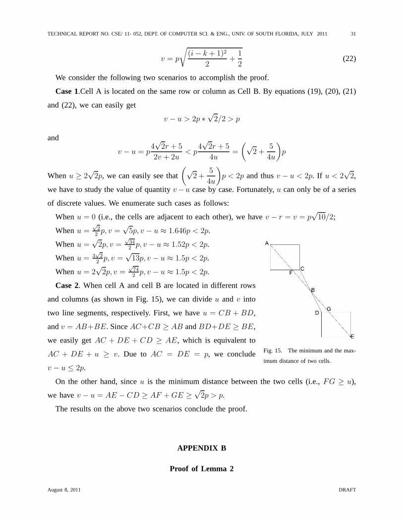
Fig. 15. The minimum and the max-
imum distance of two cells.
Whenu =√
22
p, v =√
5p, v − u ≈ 1.646p < 2p.
Whenu =√
2p, v =√
342
p, v − u ≈ 1.52p < 2p.
Whenu = 3√
22
p, v =√
13p, v − u ≈ 1.5p < 2p.
Whenu = 2√
2p, v =√
742
p, v − u ≈ 1.5p < 2p.
Case 2. When cell A and cell B are located in different rows
and columns (as shown in Fig. 15), we can divideu andv into
two line segments, respectively. First, we haveu = CB + BD,
andv = AB+BE. SinceAC+CB ≥ AB andBD+DE ≥ BE,
we easily getAC + DE + CD ≥ AE, which is equivalent to
AC + DE + u ≥ v. Due to AC = DE = p, we conclude
v − u ≤ 2p.
On the other hand, sinceu is the minimum distance between the two cells (i.e.,FG ≥ u),
we havev − u = AE − CD ≥ AF + GE ≥√
2p > p.
The results on the above two scenarios conclude the proof.
APPENDIX B
Proof of Lemma 2
August 8, 2011 DRAFT
TECHNICAL REPORT NO. CSE/ 11- 052, DEPT. OF COMPUTER SCI. & ENG., UNIV. OF SOUTH FLORIDA, JULY 2011 32
According to Table III, for any distribution operation, theerror to the first SDH bucket (denoted
as bucketi) it involves is1−F (⌊up⌋p+p), and this error is positive (i.e., overestimation). Suppose
that there is another distribution with minimum distanceu1 = u−p, then this operation generates
a negative errorF (⌊up⌋p+2p)−F (⌊u
p⌋p+p) to bucketi. For the same reason, a third distribution
with minimum distanceu2 = u− 2p generates a negative error of1− F (⌊up⌋p + 2p). It is easy
to see that the combined error (by putting all relevant negative and positive errors together) to
bucketi is 0. An example of two cells that contribute to each other’s error compensation in the
aforementioned way can be seen in Figure 6. Namely, the cellsC andC ′ when we compute the
minimum distancesAC andAC ′.
Unfortunately, the above condition of the existence of au1 value that equalsu − p cannot
be satisfied for all pairs of cells. From Lemma 2, however, we can easily see that the error is
strongly related to the quantityu.
APPENDIX C
Approximation of Triangular to Normal Distribution
Lemma 3: If X andY are independent random variables uniformly distributed on(a, b) and
(c, c + b− a), andc ≥ a, thenY −X is a triangular random variable and can be regarded as a
normal random with the relative error less than0.1.
Proof:
The probability density ofX is
f(x) =1
b− a, a < x < b (23)
and the probability density ofY is
g(y) =1
b− a, c < y < c + b− a (24)
There are two cases to be considered. One is whenc is equal toa and the other is whenc is
greater thana.
Case1: c is equal toa
The probability density ofY −X can be calculated as follows
August 8, 2011 DRAFT
TECHNICAL REPORT NO. CSE/ 11- 052, DEPT. OF COMPUTER SCI. & ENG., UNIV. OF SOUTH FLORIDA, JULY 2011 33
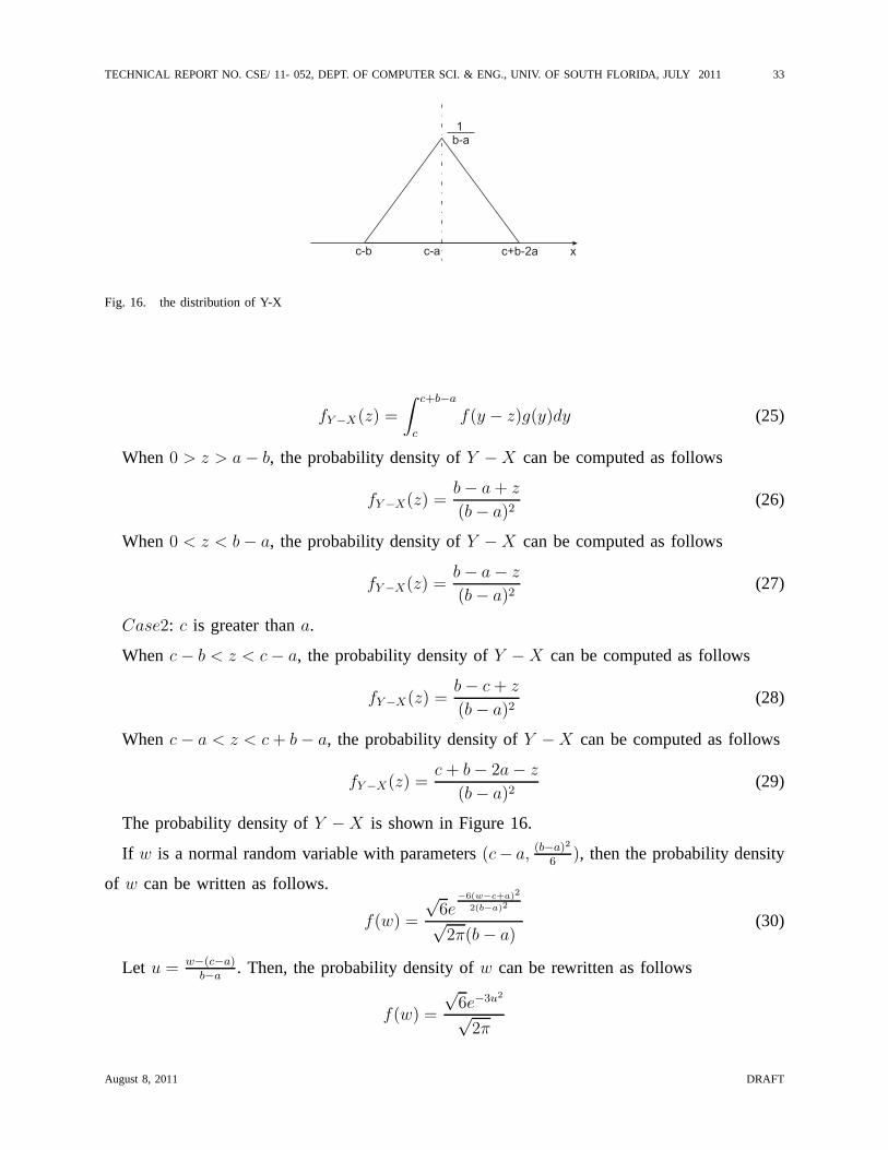
c-b c-a c+b-2a
1
b-a
x
Fig. 16. the distribution of Y-X
fY −X(z) =
∫ c+b−a
c
f(y − z)g(y)dy (25)
When0 > z > a− b, the probability density ofY −X can be computed as follows
fY −X(z) =b− a + z
(b− a)2(26)
When0 < z < b− a, the probability density ofY −X can be computed as follows
fY −X(z) =b− a− z
(b− a)2(27)
Case2: c is greater thana.
Whenc− b < z < c− a, the probability density ofY −X can be computed as follows
fY −X(z) =b− c + z
(b− a)2(28)
Whenc− a < z < c + b− a, the probability density ofY −X can be computed as follows
fY −X(z) =c + b− 2a− z
(b− a)2(29)
The probability density ofY −X is shown in Figure 16.
If w is a normal random variable with parameters(c− a, (b−a)2
6), then the probability density
of w can be written as follows.
f(w) =
√6e
−6(w−c+a)2
2(b−a)2
√2π(b− a)
(30)
Let u = w−(c−a)b−a
. Then, the probability density ofw can be rewritten as follows
f(w) =
√6e−3u2
√2π
August 8, 2011 DRAFT
TECHNICAL REPORT NO. CSE/ 11- 052, DEPT. OF COMPUTER SCI. & ENG., UNIV. OF SOUTH FLORIDA, JULY 2011 34
-1.0 -0.5 0.5 1.0
0.2
0.4
0.6
0.8
1.0
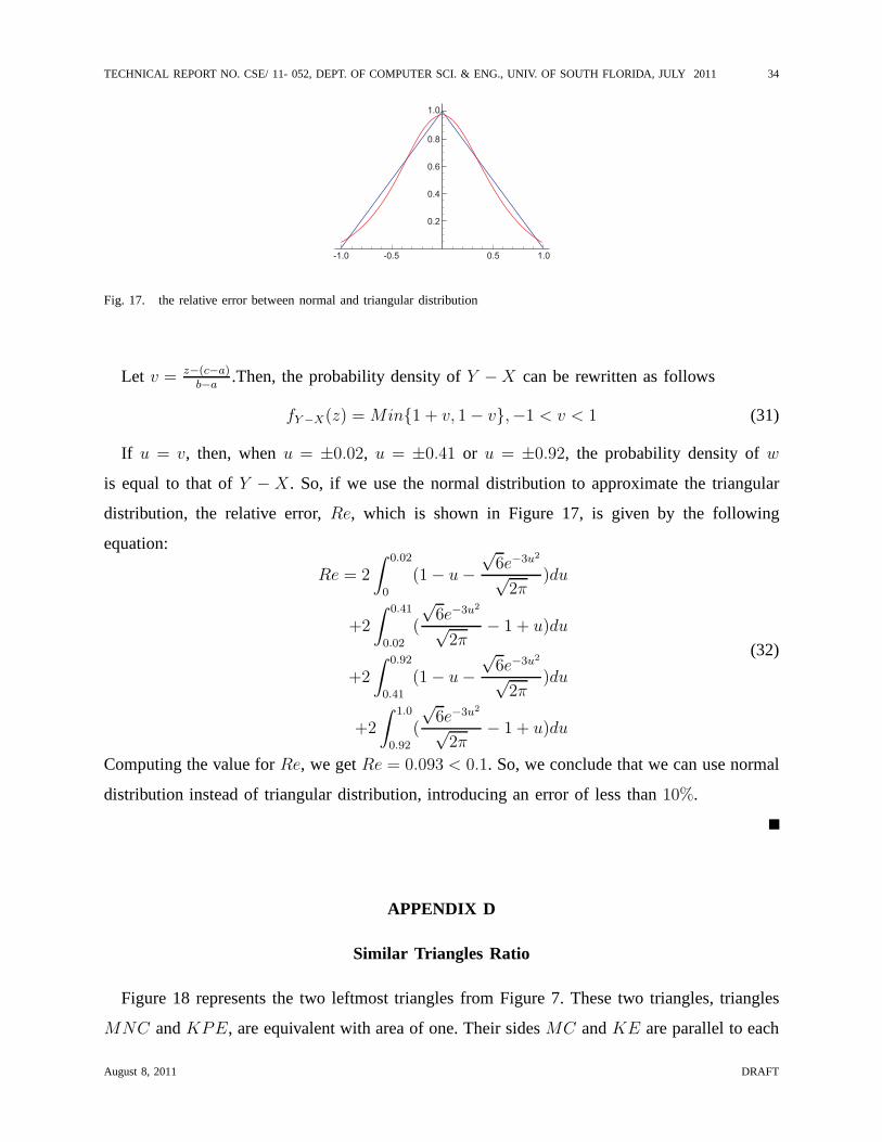
Fig. 17. the relative error between normal and triangular distribution
Let v = z−(c−a)b−a
.Then, the probability density ofY −X can be rewritten as follows
fY −X(z) = Min{1 + v, 1− v},−1 < v < 1 (31)
If u = v, then, whenu = ±0.02, u = ±0.41 or u = ±0.92, the probability density ofw
is equal to that ofY − X. So, if we use the normal distribution to approximate the triangular
distribution, the relative error,Re, which is shown in Figure 17, is given by the following
equation:
Re = 2
∫ 0.02
0
(1− u−√
6e−3u2
√2π
)du
+2
∫ 0.41
0.02
(
√6e−3u2
√2π
− 1 + u)du
+2
∫ 0.92
0.41
(1− u−√
6e−3u2
√2π
)du
+2
∫ 1.0
0.92
(
√6e−3u2
√2π
− 1 + u)du
(32)
Computing the value forRe, we getRe = 0.093 < 0.1. So, we conclude that we can use normal
distribution instead of triangular distribution, introducing an error of less than10%.
APPENDIX D
Similar Triangles Ratio
Figure 18 represents the two leftmost triangles from Figure7. These two triangles, triangles
MNC andKPE, are equivalent with area of one. Their sidesMC andKE are parallel to each
August 8, 2011 DRAFT

TECHNICAL REPORT NO. CSE/ 11- 052, DEPT. OF COMPUTER SCI. & ENG., UNIV. OF SOUTH FLORIDA, JULY 2011 35
M K N P
C E
A
B
K’
C’
Fig. 18. similar triangles
other. This imposes thatMK = CE andKK ′ = AB. Following the values from Figure 7, we
note the following:
MK = u1− u + 1 = 1−∆, MN = v − u, MC ′ = MN2
= v−u2
, CC ′ = 2MN
= 2v−u
(from the
formula of the area of the triangle:1 = 12MN ∗ CC ′).
Now, lets look at trianglesMKK ′ (the red triangle) and triangleMC ′C (the green one).
These two triangles are similar right triangles. Followingthe properties of similar triangles we
get the following:
K ′K
MK=
CC ′
MC ′ =2
v−uv−u
2
=4
(v − u)2
K ′K =4
(v − u)2∗MK
AB = K ′K =4
(v − u)2∗MK =
4
(v − u)2∗ (1−∆) (33)
APPENDIX E
Boundary situation in error compensation analysis
When the minimum distanceu is within the first bucket, i.e.u ≤ p, the error produced by
SKEW cannot be compensated in the way described in Section VI. Thereason being, there are
no buckets to the left of the first bucket, therefore the positive errors in it cannot be compensated.
August 8, 2011 DRAFT
TECHNICAL REPORT NO. CSE/ 11- 052, DEPT. OF COMPUTER SCI. & ENG., UNIV. OF SOUTH FLORIDA, JULY 2011 36
The average error caused by this, denoted aseu≤1, can be computed as follows
eu≤1 =0.3N2
2N(N − 1) + N2≈ 0.1 (34)
Therefore, by considering the Eqs. (34) and (16), the average error over all buckets of our
algorithm based on SKEW can be computed as follows:
efinal = limn→∞
eu≤1 ∗ τ + ez=0,1 ∗ (n− τ)
n= lim
n→∞
0.1 ∗ τ + 0.1055 ∗ (n− τ)
n= 0.1055 (35)
wheren is the total number of distances,τ is the number of the distances in the first bucket.
The reason for the second step of the above equation is because τ can be computed as:
τ
n= P ((x1 − x2)
2 + (y1 − y2)2 < 1) (36)
Sincex1, x2, y1 andy2 are independent variables with uniform distribution, the above proba-
bility can be shown to be very small:
P =1
2n4− 4
3n3+
3π − 4
3n2(37)
APPENDIX F
Distance distribution of particles in two cells A and B
Lemma 4: If the points in cellA and cell B are uniformly distributed, then the distances
between the two cells’ points can be described as a Noncentral chi-square distribution and the
distribution has no relationship with the number of points in cell A or cell B.
Proof:
Suppose a pointi in cell A with coordinatesxi andyi and a pointj in cell B with coordinates
is xj andyj. As we know, ifxi andxj are independent random variables uniformly distributed
on (a, b) and (c, c + b − a) respectively,(c ≥ a) thenxj − xi follows a triangular distribution.
According to the Appendix C, the triangular distribution can be approximated with normal,
introducing an error of not more than10%. Knowing this,xj − xi can be regarded as a normal
random variable with parameters(c − a, (b − a)2/6). Similarly, yj − yi can be regarded as a
normal random variable with parameters(c′ − a′, (b − a)2/6). Since(b − a)2/6 is a constant,
August 8, 2011 DRAFT
TECHNICAL REPORT NO. CSE/ 11- 052, DEPT. OF COMPUTER SCI. & ENG., UNIV. OF SOUTH FLORIDA, JULY 2011 37
which is noted asσ2, we can write the following equation for the distancel between the two
points i andj:
l2
σ2=
(xj − xi)2
σ2+
(yj − yi)2
σ2(38)
As it is known, the right hand side of the above equation is a Noncentral chi-square distribution.
This means that the distances between the two cells’ points can be described as a Noncentral
chi-square distribution with the parameters(2, λ), whereλ can be defined as follows:
λ =(c− a)2
σ2+
(c′ − a′)2
σ2(39)
wherec− a andc′ − a′ are the means of the normal distribution.
Since the parameters of Noncentral chi-square distribution have no relationship with the
number of points in cellA or cell B, the shape of the distribution of the distances is not
influenced by the points count in the cells.
So, our conclusion is that the square of the distance betweenany two points from two
cells follows (can be approximated to) a Noncentral chi-square distribution. Since the pdf of
a Noncentral chi-square distribution has a closed form which involves an infinite sum, the
pdf of the square root of Noncentral chi-square distribution can be easily obtained through
Jacobian transformation. SoE(d) can be easily worked out. However, such a closed-form is
for an approximated distribution ofd using the technique presented in Appendix C. It is our
belief, based on the thorough work we have done on this matter, that to get a closed form for
the distribution of the distances between the points of the cells is really tough and challenging,
if not impossible to solve, problem.
ACKNOWLEDGEMENTS
The project described was supported by Award Number R01GM086707 from the National Institute Of General
Medical Sciences (NIGMS) at the National Institutes of Health (NIH).
August 8, 2011 DRAFT

TECHNICAL REPORT NO. CSE/ 11- 052, DEPT. OF COMPUTER SCI. & ENG., UNIV. OF SOUTH FLORIDA, JULY 2011 38
REFERENCES
[1] J. Gray, D. Liu, M. Nieto-Santisteban, A. Szalay, D. DeWitt, and G. Heber, “Scientific Data Management in the Coming
Decade,”SIGMOD Record, vol. 34, no. 4, pp. 34–41, December 2005.
[2] A. S. Szalay, J. Gray, A. Thakar, P. Z. Kunszt, T. Malik, J.Raddick, C. Stoughton, and J. vandenBerg, “The SDSS Skyserver:
Public Access to the Sloan Digital Sky Server Data,” inProceedings of International Conference on Management of Data
(SIGMOD), 2002, pp. 570–581.
[3] M. Y. Eltabakh, M. Ouzzani, and W. G. Aref, “BDBMS - A Database Management System for Biological Data,” in
Proceedings of the 3rd Biennial Conference on Innovative Data Systems Resarch (CIDR), 2007, pp. 196–206.
[4] M. H. Ng, S. Johnston, B. Wu, S. E. Murdock, K. Tai, H. Fangohr, S. J. Cox, J. W. Essex, M. S. P. Sansom, and P. Jeffreys,
“BioSimGrid: Grid-enabled Biomolecular Simulation Data Storage and Analysis,”Future Generation Computer Systems,
vol. 22, no. 6, pp. 657–664, June 2006.
[5] J. M. Patel, “The Role of Declarative Querying in Bioinformatics,”OMICS: A Journal of Integrative Biology, vol. 7, no. 1,
pp. 89–91, 2003.
[6] S. Klasky, B. Ludaescher, and M. Parashar, “The Center for Plasma Edge Simulation Workflow Requirements,” inEEE
Workshop on Workflow and Data Flow for Scientific Applications (SciFlow’06), 1991, pp. 73–73.
[7] J. L. Stark and F. Murtagh,Astronomical Image and Data Analysis. Springer, 2002.
[8] M. P. Allen and D. J. Tildesley,Computer Simulations of Liquids. Clarendon Press, Oxford, 1987.
[9] D. Frenkel and B. Smit,Understanding Molecular Simulation: From Algorithm to Applications, ser. Computational Science
Series. Academic Press, 2002, vol. 1.
[10] J. M. Haile,Molecular Dynamics Simulation: Elementary Methods. Wiley, New York, 1992.
[11] D. P. Landau and K. Binder,A Guide to Monte Carlo Simulation in Statistical Physics. Cambridge University Press,
Cambridge, 2000.
[12] P. K. Agarwal, L. Arge, and J. Erikson, “Indexing MovingObjects,” in Proceedings of International Conference on
Principles of Database Systems (PODS), 2000, pp. 175–186.
[13] M. Bamdad, S. Alavi, B. Najafi, and E. Keshavarzi, “A new expression for radial distribution function and infinite shear
modulus of lennard-jones fluids,”Chem. Phys., vol. 325, pp. 554–562, 2006.
[14] A. Filipponi, “The radial distribution function probed by X–ray absorption spectroscopy,”J. Phys.: Condens. Matter, vol. 6,
pp. 8415–8427, 1994.
[15] B. Hess, C. Kutzner, D. van der Spoel, and E. Lindahl, “GROMACS 4: Algorithms for Highly Efficient, Load-Balanced,
and Scalable Molecular Simulation,”Journal of Chemical Theory and Computation, vol. 4, no. 3, pp. 435–447, March
2008.
[16] V. Springel, S. D. M. White, A. Jenkins, C. S. Frenk, N. Yoshida, L. Gao, J. Navarro, R. Thacker, D. Croton, J. Helly,
J. A. Peacock, S. Cole, P. Thomas, H. Couchman, A. Evrard, J. Colberg, and F. Pearce, “Simulations of the Formation,
Evolution and Clustering of Galaxies and Quasars,”Nature, vol. 435, pp. 629–636, June 2005.
[17] A. G. Gray and A. W. Moore, “N-body problems in statistical learning,” inAdvances in Neural Information Processing
Systems (NIPS). MIT Press, 2000, pp. 521–527.
[18] Y.-C. Tu, S. Chen, and S. Pandit, “Computing Distance Histograms Efficiently in Scientific Databases,” inProceedings of
International Conference on Data Engineering (ICDE), March 2009, pp. 796–807.
[19] M. Arya, W. F. Cody, C. Faloutsos, J. Richardson, and A. Toya, “QBISM: Extending a DBMS to Support 3D Medical
Images,” inICDE, 1994, pp. 314–325.
August 8, 2011 DRAFT

TECHNICAL REPORT NO. CSE/ 11- 052, DEPT. OF COMPUTER SCI. & ENG., UNIV. OF SOUTH FLORIDA, JULY 2011 39
[20] M. Stonebraker, S. Madden, D. J. Abadi, S. Harizopoulos, N. Hachem, and P. Helland, “The End of an Architectural Era
(It’s Time for a Complete Rewrite),” inVLDB, 2007, pp. 1150–1160.
[21] B. Howe, D. Maier, and L. Bright, “Smoothing the ROI Curve for Scientific Data Management Applications,” inCIDR,
2007, pp. 185–195.
[22] P. G. Brown, “Overview of scidb: large scale array storage, processing and analysis,” inSIGMOD Conference, 2010, pp.
963–968.
[23] M. Feig, M. Abdullah, L. Johnsson, and B. M. Pettitt, “Large Scale Distributed Data Repository: Design of a Molecular
Dynamics Trajectory Database,”Future Generation Computer Systems, vol. 16, no. 1, pp. 101–110, January 1999.
[24] J. Barnes and P. Hut, “A Hierarchical O(N log N) Force-Calculation Algorithm,” Nature, vol. 324, no. 4, pp. 446–449,
1986.
[25] L. Greengard and V. Rokhlin, “A Fast Algorithm for Particle Simulations ,”Journal of Computational Physics, vol. 135,
no. 12, pp. 280–292, 1987.
[26] P. B. Callahan and S. R. Kosaraju, “A decomposition of multidimensional point sets with applications to k-nearest-neighbors
and n-body potential fields,”Journal of ACM, vol. 42, no. 1, pp. 67–90, 1995.
[27] S. Chen, Y.-C. Tu, and Y. Xia, “Performance analysis of adual-tree algorithm for computing spatial distance histograms,”
The VLDB Journal, vol. 20, 2011.
[28] J. A. Orenstein, “Multidimensional Tries used for Associative Searching,”Information Processing Letters, vol. 14, no. 4,
pp. 150–157, 1982.
[29] Y.-C. Tu, S. Chen, and S. Pandit, “Computing Distance Histograms Efficiently in Scientific Databases,” inProceedings of
International Conference on Data Engineering (ICDE), March 2009, pp. 796–807.
August 8, 2011 DRAFT