Journal of Agricultural and Resource Economics 40(1):23–49 ISSN 1068-5502Copyright 2015 Western Agricultural Economics Association

On-Farm Reservoir Adoption in the Presence ofSpatially Explicit Groundwater Use and Recharge

Kent Kovacs, Michael Popp, Kristofor Brye, and Grant West

Groundwater management is conducted in spatial aquifers where well pumping results in localizedcones of depression. This is in contrast to the single-cell aquifer used in most economic analysesthat assumes groundwater depletion occurs uniformly over a study area. We address two aspectsof the optimal management of groundwater: a spatially explicit representation of the aquifer andthe potential of on-farm reservoirs to recharge the underlying aquifer. A spatial-dynamic modelof the optimal control of groundwater use and on-farm reservoir adoption is developed. Resultssuggest that a single-cell aquifer overestimates groundwater use and farm net returns over thirtyyears.

Key words: aquifer depletion, groundwater, on-farm reservoirs, spatial-dynamic optimization

Introduction

Economic studies of groundwater use have long observed a pumping cost or stock externality (Burt,1964; Brown and Deacon, 1972). The withdrawal by one user lowers the water table and increasespumping costs for all users. This externality is typically modeled to operate in a single-cell or“bathtub” aquifer (Gisser and Sánchez, 1980; Burness and Brill, 2001) in which the pumping liftis assumed to be identical for every well and the spatial location of the well is irrelevant. Brozovic,Sunding, and Zilberman (2010) demonstrate that the single-cell aquifer assumption incorrectlyestimates the magnitude of the pumping externality relative to spatially explicit models. Pfeifferand Lin (2012) find empirical evidence of a behavioral response to the spatial movement ofgroundwater in the agricultural region of western Kansas. While the potential differences in thepumping externality may be significant, the empirical ramifications for long-term groundwater useand farm profitability are left unexplored. Also, there is no investigation of how differences in the tworepresentations of the aquifer change water use and farm production results when water conservationis practiced on the landscape.

This study addresses two aspects of the optimal management of a groundwater resource. First,we examine the empirical significance of the pumping externality associated with a spatial aquiferfor groundwater depletion and farm net returns. Second, we evaluate the value of creating on-farmreservoirs to collect surface water for reuse throughout the season in the presence of a spatial aquifer.Reservoirs are allowed to recharge the aquifer, which lowers reservoir capacity but raises watertable levels sufficiently to reduce groundwater pumping costs. To address these issues, we develop a

Kent Kovacs is an assistant professor, Michael Popp is a professor, and Grant West is a program associate in the Departmentof Agricultural Economics and Agribusiness at the University of Arkansas. Kristofer Brye is a professor in the Departmentof Crop, Soil, and Environmental Sciences at the University of Arkansas.The authors thank Eric Wailes, Gregmar Galinato, two anonymous referees, and the participants of the 2013 AnnualMeeting of the Delta Region Farm Management and Agricultural Policy Working Group for helpful suggestions. Thisproject was supported by the U.S. Geologic Survey of the 104b research grant program, U.S. Department of the Interior,Grant #G11AP20066, and the University of Arkansas Division of Agriculture, Arkansas Water Resource Center, Grant#2013AR345B.

Review coordinated by Gregmar Galinato.

24 January 2015 Journal of Agricultural and Resource Economics

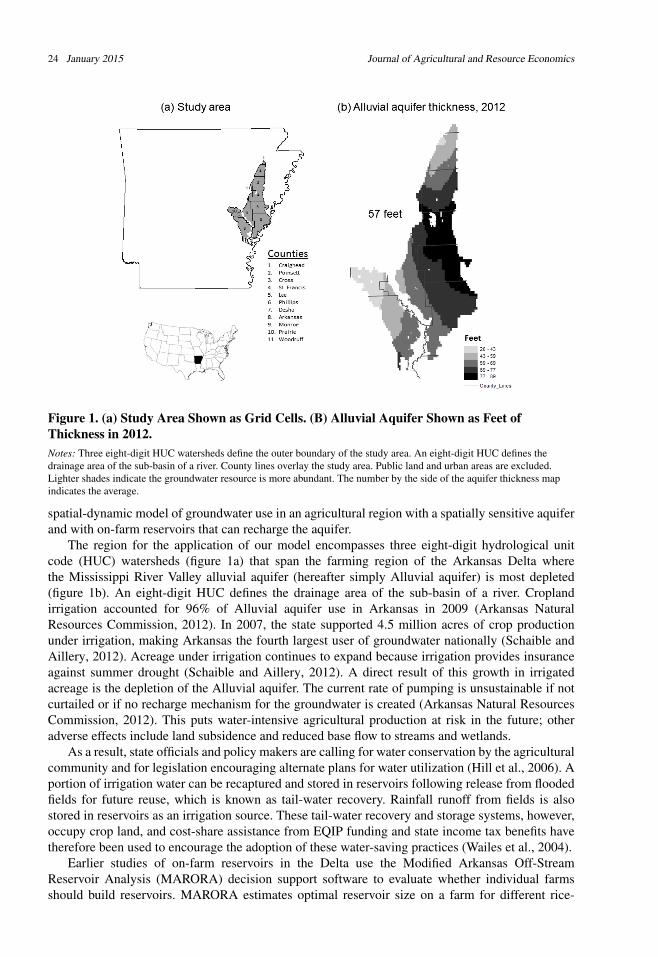
Figure 1. (a) Study Area Shown as Grid Cells. (B) Alluvial Aquifer Shown as Feet ofThickness in 2012.Notes: Three eight-digit HUC watersheds define the outer boundary of the study area. An eight-digit HUC defines thedrainage area of the sub-basin of a river. County lines overlay the study area. Public land and urban areas are excluded.Lighter shades indicate the groundwater resource is more abundant. The number by the side of the aquifer thickness mapindicates the average.

spatial-dynamic model of groundwater use in an agricultural region with a spatially sensitive aquiferand with on-farm reservoirs that can recharge the aquifer.

The region for the application of our model encompasses three eight-digit hydrological unitcode (HUC) watersheds (figure 1a) that span the farming region of the Arkansas Delta wherethe Mississippi River Valley alluvial aquifer (hereafter simply Alluvial aquifer) is most depleted(figure 1b). An eight-digit HUC defines the drainage area of the sub-basin of a river. Croplandirrigation accounted for 96% of Alluvial aquifer use in Arkansas in 2009 (Arkansas NaturalResources Commission, 2012). In 2007, the state supported 4.5 million acres of crop productionunder irrigation, making Arkansas the fourth largest user of groundwater nationally (Schaible andAillery, 2012). Acreage under irrigation continues to expand because irrigation provides insuranceagainst summer drought (Schaible and Aillery, 2012). A direct result of this growth in irrigatedacreage is the depletion of the Alluvial aquifer. The current rate of pumping is unsustainable if notcurtailed or if no recharge mechanism for the groundwater is created (Arkansas Natural ResourcesCommission, 2012). This puts water-intensive agricultural production at risk in the future; otheradverse effects include land subsidence and reduced base flow to streams and wetlands.

As a result, state officials and policy makers are calling for water conservation by the agriculturalcommunity and for legislation encouraging alternate plans for water utilization (Hill et al., 2006). Aportion of irrigation water can be recaptured and stored in reservoirs following release from floodedfields for future reuse, which is known as tail-water recovery. Rainfall runoff from fields is alsostored in reservoirs as an irrigation source. These tail-water recovery and storage systems, however,occupy crop land, and cost-share assistance from EQIP funding and state income tax benefits havetherefore been used to encourage the adoption of these water-saving practices (Wailes et al., 2004).

Earlier studies of on-farm reservoirs in the Delta use the Modified Arkansas Off-StreamReservoir Analysis (MARORA) decision support software to evaluate whether individual farmsshould build reservoirs. MARORA estimates optimal reservoir size on a farm for different rice-

Kovacs et al. Reservoirs and Spatial Aquifer Use 25

producing locations with different saturated thickness levels and groundwater decline rates (Smarttet al., 2002). Young et al. (2004) report that the thirty-year net present value (NPV) of a farmwith relatively inadequate groundwater increased by approximately $2,000 per acre with theinstallation of a reservoir. Hill et al. (2006) examine how cost-share for reservoir construction andwater diversion from the White river affects farm income and water use in the Grand Prairie ofArkansas. Farm size, crop mix, and groundwater conditions from eighty-four farms were entered intoMARORA to identify the farms where building reservoirs would be economically advantageous.

Our model accounts for spatial variation in the saturated thickness of the aquifer, the yield ofcrops, and the costs of groundwater pumping. All of these factors influence the spatial-dynamicpath of optimal management (Brozovic, Sunding, and Zilberman, 2010). The central plannermaximizes farm net returns over three decades by allocating acreage to crops and reservoirs subjectto constraints on groundwater supplies, reservoir water availability, and land availability. Spatialgroundwater flow occurs between sites in response to the distance from cones of depression formedby well pumping. The single-cell aquifer spreads the depletion of groundwater evenly over the studyarea. The boundaries of the single-cell aquifer and the study area do not exactly coincide, but thestudy area is large enough to reasonably assume that they are the same. With and without on-farmreservoirs, we compare model results for the spatial aquifer and the single-cell aquifer.

By allowing reservoirs to recharge the aquifer, we estimate the potential gains in farm net returnsattainable from lower groundwater pumping costs as a function of the lower depth to the aquifer andtherefore less energy to raise the water to the surface. The water table does not have to rise, only notfall as fast, to affect energy use over time. Even small reductions in pumping costs can translate tomeasureable gains over the long term. Groundwater provides farmers with a stable supply of water;the value of this certainty is called buffer value and is likely not considered by current farmers usinggroundwater, representing a loss to future generations. The social price of groundwater should thenreflect its risk management or stabilization value. By adding the buffer value of groundwater to theobjective, we estimate a social level of aquifer depletion and consider various policies to raise thewater table.

We describe the models for the dynamics of land and water use and the optimal control problemfaced by the planner in the next section. Data for the crop land and parameter values for the modelare presented in the third section. Section four discusses the results and sensitivity analyses. Weconclude with a summary of the major findings, relate the findings to prior work in a similar vein,and list future research needs.

Methods

Dynamics of Land and Water Use

Spatial dynamics of land and water use in the rice-soybean production region of the Delta focuson the supply of water available in the underlying aquifer. Our model follows from a map-gridrepresentation of spatially symmetric cones of depression from groundwater pumping. The modelconsists of a grid of m cells (sites) and accounts for the amount of available groundwater by timeperiod based on the pumping decisions of farms in and around the cell weighted by distance.

For each site i we track the acreage of land in use j for n land-cropping choices (rice, irrigatedsoybean, and non-irrigated soybean) at the end of period t with Li j(t). The decision to look only atrice and irrigated and non-irrigated soybeans keeps the focus on water use rather than relative cropprices. We assume that land can be converted to on-farm reservoirs FRi j(t) from existing land usej during period t, and the amount of land converted to reservoirs at the end of period t is Ri(t) ateach site. Farmers can choose to switch land out of water-intensive rice into irrigated soybeans inresponse to a growing water shortage, and this is tracked with the variable RSi(t). The declininggroundwater availability may lead farmers to switch land out of irrigated crops into non-irrigatedsoybeans; the variable tracking the land switching to non-irrigated soybean is DSi j(t). Using these

26 January 2015 Journal of Agricultural and Resource Economics

definitions, we model the dynamics of land use in each site as a system of difference equations:

Li j(t) = Li j(t − 1)− FRi j(t)− DSi j(t)− RSi(t), for j = rice

Li j(t) = Li j(t − 1)− FRi j(t)− DSi j(t) + RSi(t), for j = irr. soybean(1)

Li j(t) = Li j(t − 1)− FRi j(t) + ∑nj=1 DSi j(t), for j = non-irr. soybean

(2) Ri(t) = Ri(t − 1) +n

∑j=1

FRi j(t)

In each period, the amount of irrigated land in use j is reduced by the amount of land convertedto on-farm reservoirs or switched into non-irrigated soybean production. For cropland in rice (themost water-intensive irrigated crop), a switch to irrigated soybean (a less irrigation-intensive crop)can also occur where the decline in rice is offset by the increase in irrigated soybean. The amount ofland in non-irrigated soybeans by the end of period t is the amount of land in non-irrigated soybeansin earlier periods and the sum of the land added to non-irrigated soybean from all land uses j lessthe land converted to on-farm reservoirs during period t (equation 1). The amount of land in on-farmreservoirs by the end of period t is the amount of land in reservoirs in earlier periods and the sum ofthe amount of land added to reservoirs from all land uses j during period t (equation 2). The totalamount of land converted to a reservoir from land use j must be less than the amount of land in usej as of period t − 1: FRi j(t)≤ Li j(t − 1).

Irrigation demand in acre-feet is given by wd j, representing average annual irrigation needs forcrop j. We assume the annual irrigation applied to crop j cannot be adjusted. Purcell, Edwards,and Brye (2007) find the yield response of soybeans to irrigation was linear, suggesting that anacre-inch applied, depending on weather and location, will yield a fixed extra yield regardless ofthe level of irrigation. A profit-maximizing producer would then either fully irrigate or go withrain-fed production depending on the marginal cost of pumping (MCP) and the marginal valueproduct (MVP) of soybeans. The producer chooses to fully irrigate as long as MVP>MCP. TheMVP increases for later season applications of water as late-season irrigation provides sufficientwater to increase seed size and/or seed fill and hence yield. A producer that has started to irrigatewould thus want to reap the final benefit. The variable AQi(t) is the amount of groundwater (acre-feet) stored in the aquifer beneath site i at the end of the period t. The amount of water pumped fromthe ground is GWi(t) during period t, and the amount of water pumped from the on-farm reservoirsis RWi(t). The natural recharge (acre-feet) of groundwater at a site i from precipitation, streams, andunderlying aquifers in a period is nri and is independent of crops grown on site i.

The reservoirs can be constructed to allow some ponded water to infiltrate through the soil andrecharge the aquifer rather than lining the reservoir with a layer of clay to minimize seepage. Theamount of water that an acre of reservoir can recharge the aquifer is ri, which depends on theunderlying soil present at site i. The runoff from site i is diverted to reservoirs through a tail-waterrecovery system. A reservoir, making up a small portion of acres available in site i, can be completelyfilled from the runoff collected from site i. A larger reservoir occupying a larger fraction of site i isonly partly filled because the reservoir receives the same acre-feet of runoff.

Hence, the acre-feet of water an acre of reservoir can hold at full capacity from runoff throughoutsite i is ωmax. The water accumulated from rainfall into the reservoir is ωmin per acre. Thevalues for ωmax and ωmin are based on evaporation, rainfall, and the timing of rainfall during theseason. We define the following function for the acre-feet of water stored in an acre of reservoir:(ωmax + ωmin)− ωmax

∑nj=1 Li j(0)

Ri(t)− ri, which depends on the number acres of the reservoir Ri(t), the

total acreage of the farm field at site i, ∑ j Li j(0) with starting crop mix at t = 0, and the seepage ofwater from the reservoir to recharge the aquifer ri. Allowing the seepage of reservoir water appearscounterproductive because the water is pumped from the ground later at greater expense, but the

Kovacs et al. Reservoirs and Spatial Aquifer Use 27

advantage of infiltration is the storage of water in the aquifer for use at a later date when water ismore limited.

The function for the acre-feet of water stored in an acre of reservoir can be rewritten asωmax

(1− Ri(t)

∑nj=1 Li j(0)

)+ (ωmin − ri). This shows that the acre-feet of water held by an acre of

reservoir ranges from a low of (ωmin − ri), when the reservoir occupies the entire field and onlyannual rainfall fills the reservoir minus the infiltration, to a high of ωmax + (ωmin − ri) for areservoir so small that tail-water recovery provides plenty of water to completely fill the reservoir.As the reservoir occupies more of the field, the term

(1− Ri(t)

∑nj=1 Li j(0)

)approaches zero because less

recovered water is available to fill the reservoir to the maximum.Further, we define pik as the expected proportion of the groundwater in the aquifer that flows

underground out of site i into the aquifer of site k when an acre-foot of groundwater is pumpedout of site k, where pik is based on the distance between sites i and k, the saturated thickness, andhydraulic conductivity of the aquifer. The amount of water leaving site i is then ∑

mk=1 pikGWk(t).

The cost of pumping an acre-foot of groundwater to the surface at site i during period t is GCi(t).Pumping costs depend on the cost to lift one acre-foot of water by one foot using a pump, cp,the initial depth to the groundwater within the aquifer, d pi, and the capital cost per acre-foot ofconstructing and maintaining the well, cc. Note that we assume a producer drills a well deeper thanthe depth to the aquifer to allow for the eventual decline in the water table. Pumping costs vary bythe energy required to lift water to the surface. The possibility of new well drilling in cases wherethe aquifer level drops below the initial drilled depth is captured in the capital cost per acre-foot.The dynamics of water use and pumping cost at each site is then represented by

(3)n

∑j=1

wd jLi j(t)≤GWi(t) + RWi(t);

(4) RWi(t)≤

((ωmax + ωmin)−

ωmax

∑nj=1 Li j(0)

Ri(t)− ri

)Ri(t);

(5) AQi(t) = AQi(t − 1)−m

∑k=1

pikGWk(t) + riRi(t) + nri;

(6) GCi(t) = cc + cp

(d pi +

(AQi(0)− AQi(t))∑

nj=1 Li j(0)

).

In each period, the total amount of water for irrigating crops grown at the site must be less thanthe water pumped from the aquifer and the reservoirs (equation 3), and the amount of water availablefrom reservoirs must be less than the maximum amount of water that all the reservoirs built on thesite can hold (equation 4). The cumulative amount of water in the aquifer by the end of period t isthe amount of water in earlier periods plus the amount of recharge that occurs naturally and by thereservoirs less the amount of water pumped from surrounding sites weighted by the proximity to sitei (equation 5).

Farm Net Benefits Objective

In the absence of available information on the location and size of individual farms under thedirection of a particular farm manager and the location and size of existing wells, we makesimplifying assumptions about the optimal construction of on-farm reservoirs subject to land-and water-use constraints. We set the size of each cell to 600 acres comprising ∑ j Li j(0) acresin field crops and the remainder in natural landscape, farmsteads, and public lands. The existing

28 January 2015 Journal of Agricultural and Resource Economics

well capacity and pumping equipment only supports the current crop mix Li j(0) with ongoingpayments made for this equipment. Investment in reservoirs and a tail-water recovery systemincludes additional pumping equipment for moving water from the tail-water recovery system intothe reservoir and from the reservoir to the existing irrigation system at each site as well as annualmaintenance costs. The overall objective is then to maximize the net benefits of farm production lessthe costs of reservoir construction and use over time.

Several economic parameters are needed to complete the formulation. The price per unit of thecrop is pr j and the cost to produce an acre of the crop is ca j, which depends on the crop, j. Theyield of crop j per acre is yi j at site i. The net value per acre for crop j is then pr jy j − ca j, excludingdifferential water pumping cost between well and reservoir water and the reservoir constructioncosts. The discount factor to make values consistent over time is δt . The annual per acre cost ofconstructing and maintaining a reservoir is cr, and the cost of pumping an acre-foot of water fromthe tail-water recovery system into the reservoir and from the reservoir to the field plus the capitalcost per acre-foot of constructing and maintaining the pump is crw.

The problem is to maximize net benefits of farm production:(7)

maxFRi j(t), GWi(t),DSi j(t), RWi(t)

:T

∑t=1

δt

(m

∑i=1

∑,nj=1 (pr jyi j − ca j)Li j(t)− crFRi j(t)− crwRWi(t)− GCi(t)GWi(t)

)

subject to

(8) Li j(0) =: Li j0 , Ri(0) = 0, AQi(0) = AQi

0;

(9) FRi j(t)≥ 0, Li j(t)≥ 0, AQi(t)≥ 0;

and the spatial dynamics of land and water use (equations 1–6). The objective (equation 7) is todetermine Li j(t), FRi j(t), RWi(t), and GWi(t) (i.e., the number of acres of each crop, the number ofacres of reservoirs, and water use) to maximize the present value of net benefits of farm productionover the fixed time horizon T . Solving an infinite horizon problem with more than 2,900 sites i isnot computationally feasible. Benefits accrue from crop production constrained by the water neededfor the crops. Costs include the construction and maintenance of reservoirs/tail-water recovery, thecapital costs and maintenance of the pumps, fuel for the pumping of water from the reservoirs orground, and all other production costs. Equation (8) represents the initial conditions of the statevariables, and equation (9) is the non-negativity constraint on land use and the aquifer as wellas nonreversibility on reservoir construction. We solve this problem with Generalized AlgebraicModeling System (GAMS) 23.5.1 using the nonlinear programming solver CONOPT from AKRIConsulting and Development.

Optimality Conditions

The problem of the collective of farmers (equation 7) is used to examine how much land to convertto reservoirs for two cases. The first case assumes finite lateral flow of groundwater as describedby equation (5), and the second case is of infinite lateral flow of groundwater (i.e., the single-cellaquifer). Based on the necessary conditions for equation (7) derived in the appendix, the amount ofland converted to reservoir depends on the magnitude of groundwater pumping, which is affected bythe degree of water flow underground. Lastly, the effect of allowing recharge of the aquifer throughreservoirs on the land converted to reservoirs is evaluated.

Kovacs et al. Reservoirs and Spatial Aquifer Use 29

The condition for the optimal acres to turn into on-farm reservoirs, FRi j(t), from crop j at site iis

δtwd jGCi(t) + δtGCi(t)∂RWi(t)∂FRi j

+ λiR(t) =

(10)

δt(cr + (pr jyi j − ca j)) + δtcrw ∂RWi(t)∂FRi j

+ λi jL (t).

The term ∂RWi(t)∂FRi j

is positive because more acres converted to a reservoir means more reservoir wateravailable for the crops on the remaining land. Equation (10) indicates that the farm collective shouldconvert land to reservoirs until the marginal benefit of more reservoirs, shown on the left-hand sideof the equation (10), equals the marginal cost of more reservoirs, shown on the right-hand side ofequation (10).

The marginal benefit of another acre in reservoir is the present value of the avoided groundwaterpumping costs since crop j is not grown, δtwd jGCi(t), plus the present value of the avoidedgroundwater pumping costs from more reservoir water, δtGCi(t)

∂RWi(t)∂FRi j

, plus the shadow value

of reservoir land λ iR(t). The marginal cost of another acre of reservoir is the present value of the

construction cost crand the loss of crop j profit pr jyi j − ca j, plus the present value of the pumpingcosts to use the reservoir water, crw ∂RWi(t)

∂FRi j, and the shadow value of not having site i in crop j,

λi jL (t)).

Next, we show how the degree of lateral flow within the aquifer influences theoptimal number of reservoirs. This is done by examining the necessary conditions ofequation (7) for groundwater pumping, GWi(t), in the cases of finite and the single-cell flow of groundwater. With finite lateral flows, the condition for groundwater pumpingcan be solved as δt

(∑

nj=1

(pr jyi j−ca j)wd j

+ crw − ∑mk=1

cp pki∑

nj=1 Li j(0)

GWk

)− ∑

mk=1 λ k

AQ(t)pki = δtGCi(t).

With single-cell lateral flows, the corresponding condition for groundwater pumping isδt

(∑

nj=1

(pr jyi j−ca j)wd j

+ crw)− λAQ(t) = δtGCi(t). The marginal benefit of groundwater pumping can

be less under the assumption of finite lateral flows aquifer because groundwater pumping at site iinfluences the pumping costs of nearby sites. As slower depletion of the aquifer occurs, the need forreservoirs is diminished. Looking at the left-hand side of equation (10), higher optimal groundwaterpumping costs with the single-cell aquifer mean that more reservoirs are built.

The condition for the flow of the shadow value of the aquifer (i.e., the most the farm collectivewould pay for another acre-foot of water in the aquifer) with and without the spatial representationof the aquifer provides another perspective on why different acres of reservoirs are built foreach type of aquifer. First, the condition for AQi(t) when the aquifer is spatially segmented isλ i

AQ =−HAQi = δtcp GWi(t)∑

nj=1 Li j(0)

. Second, the condition for AQ(t) when the aquifer is a single cell is

λAQ =−HAQ = δtcp∑

mi=1

GWi(t)∑

nj=1 Li j(0)

. Greater groundwater pumping in the single-cell aquifer means

that the shadow value of the single-cell aquifer is rising faster than the shadow value of an aquiferassumed to have finite lateral flow. The greater rise of shadow value in the single-cell aquifer meansthat farms turn faster to the construction of reservoirs for cheaper water.

When reservoirs can recharge the aquifer, equation (10) changes to

δtwd jGCi(t) + δtGCi(t)∂RWi(t)∂FRi j

+ λ iR(t) + λ i

AQ(t)ri =(11)

δt(cr + (pr jyi j − ca j)) + δtcrw ∂RWi(t)∂FRi j

+ λi jL (t).

The value of the additional aquifer water, λ iAQ(t)ri, suggests that more land should be made into

reservoirs, but the reduction in irrigation water held by reservoirs suggests that less land should be

30 January 2015 Journal of Agricultural and Resource Economics

converted to reservoirs compared to the model in which reservoirs do not need to recharge becauseof the nonpermeable clay layer that prevents seepage.

Buffer Value Objective

Groundwater provides farmers with a stable supply of water that represents a value beyond thatof a supplement to non-irrigated crop production. The economic value of this risk managementor stabilization role is called buffer value. Tsur (1990) defines buffer value, BV , as the amount agrower facing an uncertain surface water supply would be willing to pay for groundwater above thecorresponding amount the grower would be willing to pay had surface water supplies been certain(or certainty equivalent).

Let the uncertain supply of surface water, S, be distributed according to a cumulative distributionhaving mean µ and variance σ2. In the absence of groundwater, growers use the surface wateravailable and enjoy the operating profit per acre of pF(S), where F() represents per acre yieldresponse to water and p is the net unit value of the crop. Tsur (1990) shows that buffer value isBV (p,µ) = pF(µ)− pE{F(S)}. By expanding F(S) about µ , BV can then be approximated byBV ∼= 0.5p[−F ′′(µ)]σ2. This indicates that BV depends on the value of marginal productivity ofwater at µ , the degree of concavity of F at µ , and the variance of surface water supply σ2. Weassume that BV remains constant over time for each acre-foot of water left in the ground.

We augment equation (7), our objective function, to include the buffer value of groundwater. TheNPV of the buffer value of the groundwater is

(12) BVT

∑t=1

δt

m

∑i=1

AQi(t).

The buffer value objective is then equation (7) plus equation (12) and hence net benefits accrue fromfarm production as well as groundwater stocks.

Sensitivity Analyses

To evaluate the impact of tail-water recovery/reservoir systems, groundwater depletion, and thebuffer value of the aquifer, model outcomes at different times are compared to the initial crop-acreage allocation for 2012. Model runs were performed by i) allowing the building of reservoirsor not by setting ∑FRi j = 0; ii) allowing the spatially differentiated movement of groundwater ornot by changing equation (5) to AQ(t) = AQ(t − 1)− ∑

mi=1(GWi(t) + nri) such that the pumped

groundwater affects the pumping cost of all sites uniformly; iii) adding a buffer value to the objectivefunction or not; iv) allowing the reservoirs to recharge the aquifer or not by setting ri to zero inequations (4) and (5); and v) evaluating policy options for groundwater conservation that includecost share for reservoir construction by modifying cr, subsidizing reservoir pumping cost crw, ortaxing groundwater pumping cost GC.

Data

The study area includes three eight-digit HUC watersheds (L’anguille, Big, and the Lower White)1

that represent the region of the Arkansas Delta where unsustainable groundwater use is occuring(figure 1a). The watersheds overlap eleven Arkansas counties: Arkansas, Craighead, Cross, Desha,Lee, Monroe, Phillips, Poinsett, Prairie, St. Francis, and Woodruff. The study area is divided into2,973 sites to evaluate how farmers make decisions about crop allocation and water use in a spatiallydifferentiated landscape. The 2010 Cropland Data Layer (Johnson and Mueller, 2010) determines

1 The HUCs for L’anguille, Big, and the Lower White are 08020205, 08020304, and 08020303.

Kovacs et al. Reservoirs and Spatial Aquifer Use 31

Table 1. Descriptive Statistics of the Model Data across Study Area Sites (n=2,973)Variable Definition Mean Std. Dev. Sum (thousands)Li,rice Initial acres of rice 123 116 366Li,irrsoy Initial acres of irrigated soybean 184 103 548Li,non−irrsoy Initial acres of dry land soybeans 59 63 174yi,rice Annual rice yield (cwt per acre) 69 3 -Yi,irr−soy Annual irrigated soybean yield (bushels per acre) 42 3 -yi,non−irrsoy Annual non-irrigated soybean yield (bushels per acre) 26 4 -d pi Depth to water (feet) 57 31 -AQi Initial aquifer size (acre-feet) 27,587 12,514 82,016K Hydraulic conductivity (feet per day) 226 92 -ri Annual aquifer recharge from an acre of reservoir (acre-feet) 0.04 0.06 -nri Annual natural recharge of the aquifer per acre (acre-feet) 0.001 0.04 547

the initial acreage of rice and soybeans in each cell (table 1), and the irrigated versus non-irrigatedsoybean acreage is allocated on the basis of harvested acreage for 2010–2011 (Arkansas Field Office,2011). The 2% real discount rate chosen for the analysis corresponds to the 5% average yield of thethirty-year Treasury bond over the last decade (U.S. Department of the Treasury, 2012) less a 3%inflation expectation. County crop-yield information for the past five years is used as a proxy foryields of each of the crops and not adjusted over time. The cost of production for all crops and theownership and maintenance charges for reservoirs and wells are also held constant.

Groundwater Use and Recharge

The depth to the water table (from surface to the top of the water table) and initial saturatedthickness (height of aquifer) of the Alluvial aquifer shown in table 1 come from the ArkansasNatural Resources Commission (Arkansas Natural Resources Commission, 2012). A thinner aquifersuggests greater depletion of the aquifer has occurred in that area (figure 1b). The initial size of theaquifer, AQi(0), at site i is computed as the acreage, ∑ j Li j(0), times the saturated thickness of theaquifer. The natural recharge, nri, of the Alluvial aquifer is based on a calibrated model of rechargefor the period 1994 to 1998 associated with precipitation, flow to or from streams, and groundwaterflow to or from the underlying Sparta aquifer (Reed, 2003). Note that producers do not have accessto the Sparta aquifer in this analysis because the greater depth to the Sparta aquifer makes pumpingfrom the Sparta prohibitively expensive and municipalities use the Sparta for drinking water.

Groundwater pumping reduces the size of the aquifer for the grid cell with the pumped well andfor the cells that surround the well. After pumping, some of the water in the aquifer flows from thesurrounding cells into the cell with the pumped well. The size of the underground flow of water isbased on the distance from the pump and the hydraulic diffusivity of the aquifer. Jenkins (1968)introduced a term that is widely applied in aquifer depletion problems called the “aquifer depletionfactor” (ADF) to quantify the relationship between these two variables. The depletion factor forpumping at a particular location in an aquifer is defined as

(13) ADF =Dd2 ,

where d is the shortest distance between the pumped well and the nearby aquifer and D is thehydraulic diffusivity of the aquifer. The hydraulic diffusivity is the ratio of the transmissivity and thespecific yield of the unconfined Alluvial aquifer (Barlow and Leake, 2012). Specific yield, whichdoes not vary across cells in our study area, is a dimensionless ratio of water drainable by saturatedaquifer material to the total volume of that material. The product of hydraulic conductivity andsaturated thickness is the transmissivity, and hydraulic conductivity is the rate of groundwater flowper unit area under a hydraulic gradient (Barlow and Leake, 2012). The hydraulic conductivity in

32 January 2015 Journal of Agricultural and Resource Economics

feet per day for the Mississippi River Valley alluvial aquifer comes from spatially coarse pilot pointsdigitized in Clark, Westerman, and Fugitt (2013).

The depletion of the aquifer beneath the cell is greater (i.e, has a large ADF) if the grid cellis closer to the pumped well and the hydraulic diffusivity is bigger. We use ADF to determine theproportion (or spatial weight) of the acre-feet of water pumped from a well that reduces the aquiferbeneath the surrounding cells. The distance from the well and hydraulic diffusivity (based on thesaturated thickness and hydraulic conductivity) of the surrounding cells influence the pik used inthe economic model. The table of the supplementary material indicates that incorporating hydraulicconductivity into spatial weights has minimal influence on the model results since the hydraulicconductivity does not vary much over the study area.

Water seepage from a reservoir into the underlying soil is estimated using soil-specific dataassigned to each cell from the Soil Survey Geographic Database (SSURGO) (Soil Survey Staff,Natural Resources Conservation Service, and US Department of Agriculture, 2012). The averagesaturated hydraulic conductivity (Ksat) for the soil-mapping unit assigned to each cell is extractedfrom SSURGO. Saturated hydraulic conductivity values extracted from SSURGO are adjusted toapproximate 10% of the estimated Ksat based on the soil surface texture of the soil mapping unitin each cell (Saxton et al., 1986). The adjusted Ksat values are assumed to reasonably represent theability of unsaturated soil to transmit water over the course of one year. The hydraulic gradient isestimated based on an average of four acre-feet of constant ponded water at the soil surface in areservoir that can be filled up to eleven feet high (the level of water in the reservoir fluctuates overthe season) and the estimated depth to the groundwater table. Annual seepage from the reservoir intothe underlying soil is then estimated as the product of the unsaturated hydraulic conductivity and thehydraulic gradient.

Farm Production

Table 2 indicates the costs of production by crop from the 2012 Crop Cost of Production estimates(Division of Agriculture, 2012). Variable irrigation costs regardless of water source include fuel,lubricant and oil, irrigation labor, and poly pipe for border irrigation plus the levee gates for theflood irrigation of rice (Hogan et al., 2007). Capital costs associated with wells, pumps, gearheads,and power units are charged on a per acre-foot basis and are incurred whether reservoirs are installedor not, as wells remain to cover potential reservoir shortfalls. The average water use over the courseof the growing season (excluding natural rainfall) is about one acre-foot for soybeans and morethan three acre-feet for rice (Powers, 2007). Crop prices are the five-year average of Decemberfutures prices for harvest time contracts for all crops (Great Pacific Trading Company, 2012). Costof production, crop price, and yields do not vary over time.

The cost of pumping water from the ground and/or reservoir depends on the costs of the fuel,maintenance, and capital. The capital cost of the well, pump and gearhead, and power unit isamortized (Hogan et al., 2007) and divided by the acre-feet pumped from the well to calculate acapital cost per acre-foot applied. The reservoir and tail-water recovery system capital cost is alsoconverted to periodic payments and depends on the reservoir acreage. The fuel cost per acre-foot ofwater from the aquifer depends on the depth to the water table and the corresponding fuel neededto raise water. Diesel use ranges from thirteen gallons of diesel per acre-foot for a 100-foot well totwenty-six gallons of diesel per acre-foot for a 200-foot well (Division of Agriculture, 2012). Thediesel needed per acre-foot for pumping water to and from the reservoir is six gallons (Hogan et al.,2007). We use $3.77 per gallon of diesel fuel (Energy Information Administration, 2012) and add10% to fuel cost to account for oil and lubricant for irrigation equipment (Hogan et al., 2007).

Kovacs et al. Reservoirs and Spatial Aquifer Use 33

Table 2. Value of Model ParametersParameter Definition Valueprrice Price of rice ($/cwt) 14.06prsoy Price of soybeans ($/bushel) 11.56carice Annual production cost of rice ($/acre) 692.3cairrsoy Annual production cost of irrigated soybeans ($/acre) 354.3canon−irrsoy Annual production cost of non-irrigated soybeans ($/acre) 299.1wdrice Annual irrigation per acre rice (acre-feet) 3.34wdsoybean Annual irrigation per acre soybean (acre-feet) 1.00Tmax Annual maximum capacity of a one acre reservoir (acre-feet) 11Tmin Annual minimum holding of a one acre reservoir (acre-feet) 1.375cr Estimated annual per acre cost of reservoir ($/acre) 96.7a

crw Cost to re-lift an acre-foot to and from the reservoir ($/acre-foot) 22.62cp Cost to raise an acre-foot of water by one foot ($/foot) 0.55δt Discount factor 0.98BV Buffer value of groundwater ($/acre-foot) 5.19

Notes: a This is the amortized cost to construct an additional acre of reservoir. The first acre of the reservoir constructed is more expensive andthe last acre of reservoir constructed is less expensive.

Reservoir Use and Construction

Young et al. (2004) determined that 440 acre-feet is the maximum a reservoir can be filled using atail-water recovery system from the average rainfall runoff on a 320-acre farm. This suggests thatan acre of land can yield 16.5 acre-inches for holding at the reservoir. This is the minimum amountof water (ωmin) that we estimate an acre of reservoir can hold without the collection of runoff froma tail-water recovery system. The use of a tail-water recovery system allows a reservoir to fill to anestimated maximum capacity of eleven acre-feet per acre over the course of a year (Smartt et al.,2002). The reservoir’s capacity is 1.5 times the storage height less what is lost to evaporation becauserunoff collected during the year refills the reservoir.

On-farm reservoir/tail-water recovery construction and maintenance costs for various reservoirsizes were estimated using MARORA (Smartt et al., 2002) for different size operations to obtaincapital-cost estimates. Subsequently, total system cost was regressed against acres occupied by thereservoir to determine per acre investment cost for different reservoir sizes. Since a majority ofthe construction cost for a reservoir rests on the cost to move one cubic yard of soil, this cost wasupdated from $1 per cubic yard to $1.20 per cubic yard to reflect changes in fuel costs since 2002,when MARORA costs were last updated. The remainder of the investment and maintenance cost isbased on estimates provided within MARORA and includes a pump for tail-water recovery and apump for irrigation.

Note that while reservoirs already exist in the study region, we assume zero reservoirs in thebaseline to highlight the potential for reservoirs. This is because of the scarcity of spatially explicitdata on existing reservoirs as well as the objective to highlight how construction of surface waterreservoirs for both irrigation use and aquifer recharge are important to farm profitability and potentialgroundwater maintenance.

Buffer Value

Using monthly rainfall data from June to September collected from the National Oceanic andAtmospheric Administration’s (NOAA) weather station in Wynne, Arkansas, for thirteen yearsfrom 2000 to 2012, the average seasonal rainfall µ is 12 inches and the variance of the seasonalrainfall, σ2, is 19.4 inches2 (National Climatic Data Center, National Oceanic and AtmosphericAdministration, 2014).

34 January 2015 Journal of Agricultural and Resource Economics

Table 3. Initial, 2022, and 2042 rr Conditions, and Farm Profits without Reservoirs for theSingle-Cell and Spatial Aquifers

Single Cell SpatialCrop and Water Conditions Initial, 2012 2022 2042 2022 2042Rice (thousand acres) 366 157 150 132 93Irrigated soybeans (thousand acres) 548 872 853 908 890Non-irrigated soybeans (thousand acres) 174 59 84 48 106Annual groundwater use (thousand acre-feet) 1,901 1,531 1,489 1,481 1,327Aquifer (thousand acre-feet) 82,016 72,180 53,340 72,679 56,487Average depth to aquifer (feet) 57.3 64.7 80.1 64.3 77.5Annual farm net returns (millions in 2012$) 114 122 109 118 99Thirty-year NPV farm net returns (millions in 2012$) N/A 2,335 2,224

Notes: All models have no buffer value for the groundwater.

Several functional forms are estimated for the response of soybean yield to water input, and thenatural log form is chosen to determine the concavity of soybean yield response to water input at theaverage rainfall for the season, [−F ′′(µ)], roughly 0.15 bushels per acre inch2. Based on a five-yearaverage of December futures prices for harvest time contracts, the price of soybean is $11.56 perbushel (Great Pacific Trading Company, 2012) and the cost of production for a bushel of soybeansbased on Arkansas production budgets is $7.99 (Division of Agriculture, 2012), making the net unitvalue of soybeans equal to $3.57.

The buffer value of an acre-foot of groundwater used to irrigate soybeans for an average seasonis then: BV ∼= 0.5p[−F ′′(µ)]σ2 = 0.5× 3.57× 0.15× 19.4 = $5.19. We base the buffer value ofgroundwater on soybean production, which is less profitable than rice, and hence this value isconsidered a conservative estimate.

Results

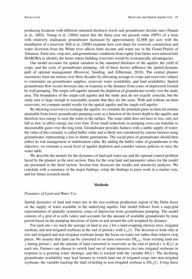
Using the single-cell aquifer and no reservoir construction, groundwater is used intensively tomaintain as many profitable rice acres as possible. Rice acreage is diverted increasingly to soybeans(table 3). The irrigated crops allow farms to maintain greater net returns, but by 2042 the depth to thewater table increases to eighty feet and only 65% of the aquifer remains (figure 2). The rice-intensiveareas are less affected by groundwater depletion with the single cell than the spatial aquifer becausethe decline of the water table is spread evenly across the entire study area. In 2042, 42% of riceacres with the single-cell aquifer remain versus only 26% of rice acres with the spatial aquifer. Lessgroundwater use with the spatial aquifer comes at the cost of fewer rice acres and lower farm netreturns (figures 3 and 4). With the spatial aquifer, farmers in the rice-intensive areas quickly increasethe depth to the water table thereby accelerating the switch to soybeans (figure 2). The model usingthe single-cell aquifer neglects the spatially explicit changes in pumping cost and overestimates thethirty-year NPV by 5%.

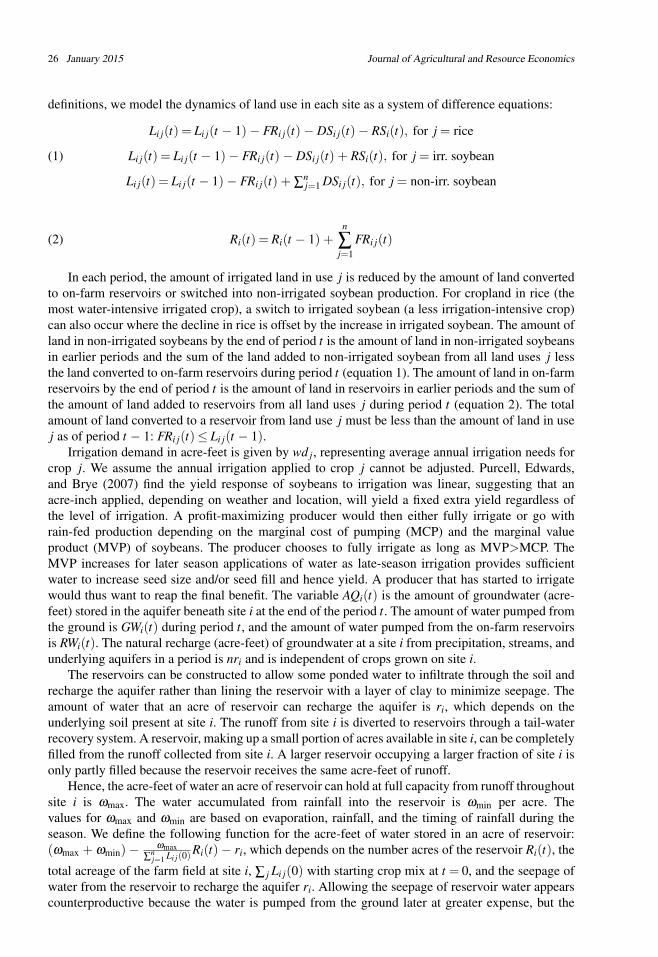
The 15–30% higher annual farm net returns with reservoirs indicate reservoir construction isworthwhile to farmers (table 4). The total aquifer volume across the region still declines over time,as does rice production, resulting in more soybean production (figure 3). Nonetheless, the addition ofreservoirs allows 91% of the aquifer and 89% of the rice acres to remain. The presence of reservoirsthus represents a cost-effective alternative to increasingly expensive groundwater use over time.Over thirty years, the use of reservoirs increases farm net returns more than 400 million comparedto no construction of reservoirs.

The use of reservoirs reduces the difference in model outcomes between the single-cell andspatial aquifer from the above 5% to 2% as the presence of reservoir water reduces the relianceon increasingly expensive groundwater over time. Reservoirs are built sooner with the spatialaquifer because the pumping of groundwater in rice-intensive areas necessitates earlier reservoir

Kovacs et al. Reservoirs and Spatial Aquifer Use 35

Figure 2. Reservoir Location under the Single-Cell and Spatial Aquifers along with AquiferDecline with and without ReservoirsNotes: Greater than 100% initial aquifer thickness is possible due to natural recharge. The numbers by the side of each mapindicate study area averages. The smaller map in the middle is the initial aquifer thickness shown in detail in figure 1.

Table 4. Initial, 2022, and 2042 Crop Allocations, Water Conditions, Reservoir Adoption, andFarm Profits with Reservoirs for the Single-Cell and Spatial Aquifers

Single Cell SpatialCrop And Water Conditions Initial, 2012 2022 2042 2022 2042Rice (thousand acres) 366 316 315 316 315Irrigated soybeans (thousand acres) 548 674 653 667 655Non-irrigated soybeans (thousand acres) 174 6 6 6 6Reservoirs (thousand acres) 0 93 114 100 112Annual reservoir water use (thousand acre-feet) 0 1,000 1,214 1,101 1,220Annual groundwater use (thousand acre-feet) 1,901 874 634 765 631Aquifer (thousand acre-feet) 82,016 78,750 75,220 79,838 77,353Average depth to aquifer (feet) 57.3 59.3 62.2 58.4 60.5Annual farm net returns (millions in 2012$) 114 141 135 138 132Thirty-year NPV farm net return (millions in 2012$) N/A 2,772 2,706

Notes: All models have no buffer value for the groundwater and allow no recharge of the aquifer from reservoirs.

construction. The availability of reservoir water allows similar acres of rice with and without thespatial aquifer. The fewer reservoirs built in 2022 with the single-cell aquifer leaves more landavailable for growing irrigated soybeans. Faster depletion of groundwater with the single-cell aquiferrequires more reservoirs be built by 2042. Reservoirs are more evenly built across the study areawith the single-cell aquifer than the spatial aquifer, but either way most reservoirs are built in rice-intensive areas (figure 2).

Table 5 shows how crop allocation, water use, and reservoir adoption change when the plannerhas the social objective to preserve the buffer value of the aquifer and reservoirs have the ability

36 January 2015 Journal of Agricultural and Resource Economics

Figure 3. Crop Acreage Allocation Changes from 2012 to 2042 for Rice and Soybean with andwithout Reservoirs Using the Spatial AquiferNotes: Rice acreage can convert to irrigated or non-irrigated soybean or farm reservoirs. Irrigated soybean acreage canconvert to non-irrigated soybean or farm reservoirs. The numbers by the side of each map indicate study area averages. Thesmaller map in the middle is the initial aquifer thickness shown in detail in figure 1.

Table 5. Initial and Final Crop Allocations, Water Conditions, Reservoir Adoption, and thePrivate and Social Net Returns with and without Buffer Values for the Groundwater andwith and without Recharge from the Reservoirs

Without Recharge With Recharge

Crop and Water Conditions Initial,2012

2042, w/oBuffer

Value (A)

2042, w/Buffer

Value (B)

2042, w/oBuffer

Value (C)

2042, w/Buffer

Value (D)Rice (thousand acres) 366 315 315 315 315Irrigated soybeans (thousand acres) 548 655 644 663 648Non-irrigated soybeans (thousand acres) 174 6 6 6 6Reservoirs (thousand acres) 0 112 124 105 120Annual reservoir water use (thousand acre-feet) 0 1,220 1,353 1,145 1,310Annual groundwater use (thousand acre-feet) 1901 631 485 716 533Aquifer (thousand acre-feet) 82,016 77,353 82,717 76,455 82,278Average depth to aquifer (feet) 57.3 60.5 56.5 61.2 56.4Annual farm net returns (millions in 2012$) 114 132 132 133 132Thirty-year NPV farm net return (millions in2012$)

– 2,706 2,669 2,710 2,670

Thirty-year NPV social net returns (millions in2012$)

– 4,567 4,606 4,568 4,607

Notes: All models use the spatial aquifer and allow on-farm reservoirs.a The buffer value of the aquifer is not counted in the farm net returns.

Kovacs et al. Reservoirs and Spatial Aquifer Use 37

to recharge the aquifer. Taking the buffer value of groundwater into account increases the volumeof the aquifer to 89,000 acre-feet by 2042 (column B in table 5). This is done by building an extra28,000 acres of reservoirs (column B vs column A), and farm net returns in 2042 only fall slightlysince nearly all the rice acres remains. The thirty-year social net returns, where the objective is thefarm net returns and the buffer value of the aquifer, are $89 million greater when preserving thegroundwater, but the thirty-year farm net returns are $85 million lower.

Not lining the bottom of reservoirs allows the collected reservoir water to recharge the aquifer(columns C and D). Farms build 8,000 fewer acres of reservoirs (column C vs column A), sinceeach reservoir is less efficient at providing water for the farm to use. The farmers thus substitutetoward the use of more groundwater, and the aquifer declines faster. Farm net returns rise slightlywhen reservoirs recharge the aquifer since fewer reservoir acres mean more irrigated cropland, andpumping costs are slightly lower from the shallower pumping depth due to the aquifer rechargeby the reservoirs. This suggests that farms can benefit when reservoirs allow recharge, althoughthe aquifer is left more depleted. When the buffer value of the groundwater is accounted for, theopposite happens. One thousand more acres of reservoirs are built, (column D vs column B), usingthe reservoir recharge to raise the water table. By accounting for the buffer value of groundwater,the groundwater stock remains close to present levels, and thus sustainability of the aquifer is anoutcome of internalizing the in situ value of groundwater. This lowers the thirty-year farm netreturns, but the social net returns increase.

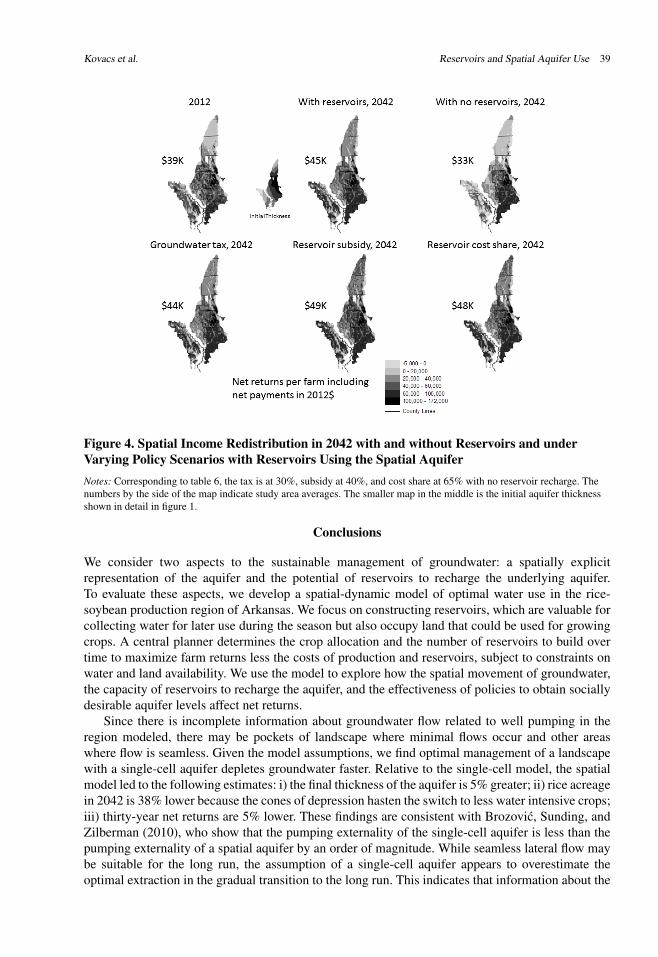
Given the positive effects of reservoirs on groundwater levels as well as on farm income, weexplore policies to speed the adoption of reservoirs by farmers in table 6. The policies modifyproducer behavior to align profit maximization with the social goal of internalizing groundwaterbuffer value in the farm production decision. This includes varying the level of cost-share ofreservoir construction, a subsidy on reservoir pumping costs, and a tax on groundwater pumping.The effectiveness of the policies is judged by the aquifer volume, farm net returns, redistributionof income between farmers and taxpayers, and conservation costs relative to the 2042 baselineoutcome. Further, we assume no aquifer recharge from reservoirs, as most reservoirs in the pasthave prevented this, for the subsidy on reservoir water and tax on groundwater. For the cost-shareprogram, we also evaluate the possibility of reservoir recharge.

Several observations are possible about the effect of the policies. One, the greater the level ofthe policy the faster is the transition to the 2042 reservoir acres. Two, cost share for reservoirs withrecharge leads to fewer 2042 acres with the 65% cost share (128,000 acres) than the 30% cost share(134,000 acres) because there are different speeds of reservoir adoption and 2042 water table levels.Three, relatively high levels of policy intervention are needed to maintain the 2012 aquifer volume.Four, the tax option has the least income redistribution. Five, the low level subsidy and tax optionsresult in greater social returns (net farm returns plus government revenue) than the baseline andhence the conservation cost per acre-foot is negative or highly cost effective. Comparing all optionson the basis of conservation cost per acre-foot, the option to cost-share reservoirs with rechargecan be eliminated. At the higher level of implementation, the cost share is the least effective atmaintaining aquifer levels at the 2012 level.

Figure 4 shows income redistribution effects without policy intervention compared to the 2012baseline as well as effects of the 30% tax, 40% reservoir pumping subsidy, and 65% reservoircost share without reservoir recharge. Exploitation of the aquifer as would be evident without theconstruction of reservoirs shows the most bleak income picture concentrated in areas where initialaquifer saturated thickness was lowest. Adding reservoirs without government intervention raisesincome levels, not only in regions initially most depleted. Comparing the center top panel (nogovernment intervention with reservoirs) with the bottom three panels, subsidies and cost shareallow for greater income in regions where the water table was initially more depleted but at a cost totaxpayers.

38 January 2015 Journal of Agricultural and Resource Economics

Tabl

e6.

Wat

erC

onse

rvat

ion

Polic

iesI

nflue

nce

onR

eser

voir

Ado

ptio

n,W

ater

Use

,and

Priv

ate

and

Publ

icR

etur

ns

Res

ervo

irA

cres

(tho

usan

d)

Res

ervo

irW

ater

(tho

usan

dac

re-f

eet)

Gro

undw

ater

(tho

usan

dac

re-f

eet)

Aqu

ifer

(tho

usan

dac

re-f

eet)

Farm

Net

Ret

urns

a

($m

illio

ns)

Gov

ernm

ent

Rev

enue

($m

illio

ns)

Con

serv

atio

nC

ostb

($/a

cre-

foot

)

Polic

yL

evel

2022

2042

2042

2042

2042

30-Y

ear

NPV

30-Y

ear

NPV

2012

Bas

elin

e10

311

21,

220

631

77,3

532,

706

0na

Cos

t-sh

are

rese

rvoi

rcon

stru

ctio

nco

sts,

nore

serv

oirr

echa

rge

30%

108

122

1,29

255

479

,196

2,76

8−

651.

3765

%11

512

41,

315

528

80,6

592,

847

−14

71.

67C

ost-

shar

ere

serv

oirc

onst

ruct

ion

cost

s,re

serv

oirr

echa

rge

30%

108

134

1,39

643

780

,376

2,76

2−

663.

1565

%11

412

81,

346

493

81,1

642,

844

−14

82.

50Su

bsid

ize

rese

rvoi

rpum

ping

fuel

cost

s,no

rese

rvoi

rrec

harg

e20

%11

211

51,

221

633

79,0

672,

816

−10

8−

1.44

40%

120

122

1,29

555

281

,655

2,92

9−

231

1.75

Tax

ongr

ound

wat

erus

e,no

rese

rvoi

rrec

harg

e10

%11

211

71,

234

617

79,1

762,

679

27−

0.04

30%

122

123

1,30

853

682

,147

2,63

461

2.20

Not

es:A

llm

odel

sha

veno

buff

erva

lue

fort

hegr

ound

wat

eran

dus

eth

esp

atia

laqu

ifer

.a

The

farm

netr

etur

nsin

clud

eth

epa

ymen

tsto

orre

ceip

tsfr

omth

ego

vern

men

tas

are

sult

ofth

epo

licy.

bC

onse

rvat

ion

cost

isca

lcul

ated

asth

edi

ffer

ence

inco

mbi

ned

farm

netr

etur

nsan

dgo

vern

men

trev

enue

rela

tive

toth

eba

selin

edi

vide

dby

the

chan

gein

aqui

ferl

evel

betw

een

the

polic

yop

tion

and

the

base

line.

For

exam

ple,

subs

idiz

ing

rese

rvoi

rcon

stru

ctio

nco

stat

30%

with

outr

eser

voir

rech

arge

led

toco

mbi

ned

farm

netr

etur

nsan

dgo

vern

men

trev

enue

of$2

,703

mill

ion

or$3

mill

ion

less

than

the

base

line.

Tha

t$3

mill

ion

cost

allo

wed

1.8

mill

ion

extr

aac

re-f

eeti

nth

eaq

uife

r(79

,196

âAS

77,3

53)r

esul

ting

ina

cost

of$1

.37/

acre

-foo

t.N

egat

ive

num

bers

impl

ygr

eate

rcom

bine

dfa

rmne

tret

urns

and

gove

rnm

entr

even

ueco

mpa

red

toth

eba

selin

e.

Kovacs et al. Reservoirs and Spatial Aquifer Use 39

Figure 4. Spatial Income Redistribution in 2042 with and without Reservoirs and underVarying Policy Scenarios with Reservoirs Using the Spatial AquiferNotes: Corresponding to table 6, the tax is at 30%, subsidy at 40%, and cost share at 65% with no reservoir recharge. Thenumbers by the side of the map indicate study area averages. The smaller map in the middle is the initial aquifer thicknessshown in detail in figure 1.

Conclusions

We consider two aspects to the sustainable management of groundwater: a spatially explicitrepresentation of the aquifer and the potential of reservoirs to recharge the underlying aquifer.To evaluate these aspects, we develop a spatial-dynamic model of optimal water use in the rice-soybean production region of Arkansas. We focus on constructing reservoirs, which are valuable forcollecting water for later use during the season but also occupy land that could be used for growingcrops. A central planner determines the crop allocation and the number of reservoirs to build overtime to maximize farm returns less the costs of production and reservoirs, subject to constraints onwater and land availability. We use the model to explore how the spatial movement of groundwater,the capacity of reservoirs to recharge the aquifer, and the effectiveness of policies to obtain sociallydesirable aquifer levels affect net returns.

Since there is incomplete information about groundwater flow related to well pumping in theregion modeled, there may be pockets of landscape where minimal flows occur and other areaswhere flow is seamless. Given the model assumptions, we find optimal management of a landscapewith a single-cell aquifer depletes groundwater faster. Relative to the single-cell model, the spatialmodel led to the following estimates: i) the final thickness of the aquifer is 5% greater; ii) rice acreagein 2042 is 38% lower because the cones of depression hasten the switch to less water intensive crops;iii) thirty-year net returns are 5% lower. These findings are consistent with Brozovic, Sunding, andZilberman (2010), who show that the pumping externality of the single-cell aquifer is less than thepumping externality of a spatial aquifer by an order of magnitude. While seamless lateral flow maybe suitable for the long run, the assumption of a single-cell aquifer appears to overestimate theoptimal extraction in the gradual transition to the long run. This indicates that information about the

40 January 2015 Journal of Agricultural and Resource Economics

spatial flow of groundwater in the aquifer is valuable to the resource planner for evaluating economicoutcomes.

Constructing reservoirs improves farm net returns by 15% or more and lessens the rate of declineof the aquifer by more than 39%. In addition, reservoirs increase the rice acreage remaining in thefinal period by more than 180%. To increase the water table to the social (buffer value) level, theacres in reservoirs must rise by 24%, but the rice acreage declines by less than 1%. This meansthirty-year net returns only decline by 3%. Allowing reservoirs to recharge the aquifer results infewer reservoirs because each reservoir provides less water, but the recharge reduces the cost ofwell pumping, actually increasing farm net returns. With the buffer value of groundwater, the useof reservoirs with recharge increases social net returns because the water table level is the largest.Regulatory programs are needed for farms to internalize the buffer value of the aquifer for futuregenerations.

We find that policies to enhance the aquifer resource differ in their effectiveness at supportingfarm net returns while limiting government income redistribution. A tax on groundwater is the mosteffective at increasing the water table and lowers farm returns marginally with minimal incomeredistribution compared to a scenario without government intervention. Since a tax is likely anunpopular scenario with policy makers, the subsidy strategy for reservoir pumping at the 20% levelprovided cost-effective support for resource conservation but was not sufficient to maintain aquiferlevels. Cost sharing with recharge, while effective at maintaining the aquifer, was not cost effective.The combination of a tax on groundwater use and potential subsidies may therefore prove worthy ofconsideration. On the basis of these results, however, it is unlikely that a single policy will lead tothe socially optimal aquifer volume of 89.6 million acre-feet.

Prior empirical analyses that examined aspects of aquifer depletion, reservoir construction, andfarm production have found different degrees of investment in reservoirs necessary to sustain thegroundwater resource. For example, studies find the thickness of the aquifer has to fall to thirty feetbefore a reservoir is needed, though the optimal size depends on crop productivity and groundwaterdecline rate (Wailes et al., 2004; Hristovska et al., 2011). Conversely, our study observes reservoirsbuilt where the aquifer is fifty feet thick. This discrepancy may be because of differences in therate of groundwater pumping predicted over time and the fuel costs involved in the well pumping.Similar to Hill et al. (2006), we find fewer than half of the farms build reservoirs without cost-share or another incentive program. We also find that, on average, nearly 10% of a farm’s acreage isoptimally converted to a reservoir.

Other lines of research can investigate the relationships among groundwater use, a spatiallyexplicit aquifer, and on-farm reservoirs. The assumption that farmers cannot adjust the irrigationapplied to a crop within a season can be relaxed. Full information on the marginal product of watercould permit an exploration of how farmers balance between less irrigation water and yield loss.Another line is how effectively reservoirs stabilize net returns under institutional arrangements otherthan optimal management. In a seminal paper, Gisser and Sánchez (1980) show that competitivepumping differs only slightly from optimal pumping in an application to the Pecos Basin in NewMexico. This result depends, among other things, on constant crop mix, constant crop requirement,constant energy costs, fixed irrigation technology, and constant hydrologic conditions (Koundouri,2004). Later papers indicate that the inefficiency from competitive (myopic) pumping is only one ofseveral externalities inherent in groundwater use. Negri (1989) develops a dynamic game-theoreticmodel of groundwater use in a common property setting to account for a strategic externality.Provencher and Burt (1993) consider risk-averse users in an environment of uncertain income returnswhere competitive groundwater use has a risk externality. These considerations are qualitativeevidence that a divergence between competitive and optimal pumping can arise, and an explorationof these differences in the context of a spatial aquifer and on-farm reservoirs is worthwhile.

In addition to the use of on-farm reservoirs, other strategies have been proposed to stabilizedeclining water tables. These strategies include cost-share assistance for “water-saving” irrigationtechnologies (Peterson and Ding, 2005; Huffaker and Whittlesey, 1995), incentive payments to

Kovacs et al. Reservoirs and Spatial Aquifer Use 41

convert irrigated crop production to dryland crop production (Ding and Peterson, 2012; Wheeleret al., 2008), tradable quotas of groundwater stock (Provencher and Burt, 1993, 1994), and theplanting of less water-intensive bioenergy crops such as switchgrass and sorghum (Popp, Nalley,and Vickery, 2010). The Arkansas Delta continues to utilize ever greater quantities of groundwaterto maintain irrigated production, including rice, which is not grown as intensively elsewhere in theUnited States. As the Alluvial aquifer continues to decline, optimal groundwater management hasthe potential to sustain the aquifer and maintain farm profitability.

[Received July 2013; final revision received September 2014.]

References

Arkansas Field Office. “Soybean Irrigated and Non-Irrigated.” 2011. Available online athttp://www.nass.usda.gov/Statistics_by_State/Arkansas/Publications/County_Estimates/.

Arkansas Natural Resources Commission. Arkansas Ground-Water Protection and ManagementReport for 2011. Little Rock, AR: State of Arkansas, 2012. Available online athttps://static.ark.org/eeuploads/anrc/2011_gw_report.pdf.

Barlow, P. M., and S. A. Leake. “Streamflow Depletion by Wells—Understanding and Managingthe Effects of Groundwater Pumping on Streamflow.” Circular 1376, U.S. Departmentof the Interior, U.S. Geological Survey, Washington, DC, 2012. Available online athttp://pubs.usgs.gov/circ/1376/.

Brown, G., and R. Deacon. “Economic Optimization of a Single-Cell Aquifer.” Water ResourcesResearch 8(1972):557–564.

Brozovic, N., D. L. Sunding, and D. Zilberman. “On the Spatial Nature of theGroundwater Pumping Externality.” Resource and Energy Economics 32(2010):154–164. doi:10.1016/j.reseneeco.2009.11.010.

Burness, H. S., and T. C. Brill. “The Role for Policy in Common Pool Groundwater Use.” Resourceand Energy Economics 23(2001):19–40. doi: 10.1016/S0928-7655(00)00029-4.

Burt, O. R. “Optimal Resource Use over Time with an Application to Ground Water.” ManagementScience 11(1964):80–93.

Clark, B. R., D. A. Westerman, and D. T. Fugitt. “Enhancements to the Mississippi EmbaymentRegional Aquifer Study (MERAS) Groundwater-Flow Model and Simulations of SustainableWater-Level Scenarios.” U.S. Geological Survey Scientific Investigations Report 2013–5161,2013. Available online at http://pubs.usgs.gov/sir/2013/5161/.

Ding, Y., and J. M. Peterson. “Comparing the Cost-Effectiveness of Water Conservation Policies ina Depleting Aquifer: A Dynamic Analysis of the Kansas High Plains.” Journal of Agriculturaland Applied Economics 44(2012).

Division of Agriculture. “2012 Crop Enterprise Budgets for Arkansas Field CropsPlanted in 2012.” Report AG-1272, University of Arkansas, Little Rock, AR,2012. Available online at http://www.themiraclebean.com/sites/default/files/attachments/Arkansas%20Crop%20Budgets%202012_0.pdf.

Energy Information Administration. Gasoline and Diesel Fuel Update. Washington, D.C.: U.S.Department of Energy, 2012. Available online at http://www.eia.gov/petroleum/gasdiesel/.

Gisser, M., and D. A. Sánchez. “Competition versus Optimal Control in Groundwater Pumping.”Water Resources Research 16(1980):638–642. doi: 10.1029/WR016i004p00638.

Great Pacific Trading Company. “Charts and Quotes.” 2012. Available online athttp://www.gptc.com/gptc/charts-quotes/.

Hill, J., E. Wailes, M. Popp, J. Popp, J. Smartt, K. Young, and B. Watkins. “Surface Water DiversionImpacts on Farm Income and Sources of Irrigation Water: The Case of the Grand Prairie inArkansas.” Journal of Soil and Water Conservation 61(2006):185–191.

42 January 2015 Journal of Agricultural and Resource Economics

Hogan, R., S. Stiles, P. Tacker, E. Vories, and K. J. Bryant. “Estimating Irrigation Costs.” Agricultureand Natural Resources Report FSA28-PD-6-07RV, University of Arkansas Cooperative ExtensionService, Little Rock, AR, 2007.

Hristovska, T., K. B. Watkins, M. M. Anders, and V. Karov. “The Impact of Saturated Thicknessand Water Decline Rate on Reservoir Size and Profit.” In R. J. Norman and J. F. Meullenet, eds.,B. R. Wells Rice Research Series, No. 591 in AAES Research Series. Little Rock, AR: ArkansasAgricultural Experiment Station, 2011, 322–326.

Huffaker, R. G., and N. K. Whittlesey. “Agricultural Water Conservation Legislation: Will It SaveWater?” Choices 10(1995).

Jenkins, C. T. “Computation of Rate and Volume of Stream Depletion by Wells.” In Techniquesof Water-Resources Investigations, Book 4, Washington, D.C.: U.S. Geological Survey, 1968.Available online at http://pubs.usgs.gov/twri/twri4d1/.

Johnson, D. M., and R. Mueller. “The 2009 Cropland Data Layer.” Photogrammetric Engineeringand Remote Sensing 11(2010):1201–1205. Available online at http://www.nass.usda.gov/research/Cropland/docs/JohnsonPE&RS_Nov2010.pdf.

Koundouri, P. “Current Issues in the Economics of Groundwater Resource Management.” Journalof Economic Surveys 18(2004):703–740. doi: 10.1111/j.1467-6419.2004.00234.x.

National Climatic Data Center, National Oceanic and Atmospheric Administration. “Climate DataOnline Search.” 2014. Available online at http://www.ncdc.noaa.gov/cdo-web/search.

Negri, D. H. “The Common Property Aquifer as a Differential Game.” Water Resources Research25(1989):9–15. doi: 10.1029/WR025i001p00009.

Peterson, J. M., and Y. Ding. “Economic Adjustments to Groundwater Depletion in the High Plains:Do Water-Saving Irrigation Systems Save Water?” American Journal of Agricultural Economics87(2005):147–159. doi: 10.1111/j.0002-9092.2005.00708.x.

Pfeiffer, L., and C. Y. C. Lin. “Groundwater Pumping and Spatial Externalities inAgriculture.” Journal of Environmental Economics and Management 64(2012):16–30. doi:10.1016/j.jeem.2012.03.003.

Popp, M. P., L. L. Nalley, and G. B. Vickery. “Irrigation Restriction and Biomass MarketInteractions: The Case of the Alluvial Aquifer.” Journal of Agricultural and Applied Economics42(2010).

Powers, S. “Agricultural Water Use in the Mississippi Delta.” Jackson, MS, 2007. Proceedings ofthe 37th Annual Mississippi Water Resources Conference: Mississippi Water Resources ResearchInstitute. Available online at http://www.wrri.msstate.edu/pdf/powers07.pdf.

Provencher, B., and O. Burt. “The Externalities Associated with the Common Property Exploitationof Groundwater.” Journal of Environmental Economics and Management 24(1993):139–158. doi:10.1006/jeem.1993.1010.

———. “A Private Property Rights Regime for the Commons: The Case for Groundwater.”American Journal of Agricultural Economics 76(1994):875–888. doi: 10.2307/1243748.

Purcell, L. C., J. T. Edwards, and K. R. Brye. “Soybean Yield and Biomass Responses to CumulativeTranspiration: Questioning Widely Held Beliefs.” Field Crops Research 101(2007):10–18. doi:10.1016/j.fcr.2006.09.002.

Reed, T. B. “Recalibration of a Groundwater Flow Model of the Mississippi River ValleyAlluvial Aquifer of Northeastern Arkansas, 1918–1998, with Simulations of Water LevelsCaused by Projected Groundwater withdrawls through 2049.” Water-Resources InvestigationsReport 03-4209, U.S. Geological Survey, Washington, DC, 2003. Available online athttp://pubs.usgs.gov/wri/wri034109/.

Saxton, K. E., W. J. Rawls, J. S. Romberger, and R. I. Papendick. “Estimating Generalized Soil-Water Characteristics from Texture.” Soil Science Society of America Journal 50(1986):1031–1036. doi: 10.2136/sssaj1986.03615995005000040039x.

Kovacs et al. Reservoirs and Spatial Aquifer Use 43

Schaible, G. B., and M. P. Aillery. “Water Conservation in Irrigated Agriculture: Trends andChallenges in the Face of Emerging Demands.” Economic Information Bulletin 99, U. S.Department of Agriculture, Economic Research Service, Washington, D.C., 2012. Availableonline at http://www.ers.usda.gov/publications/eib-economic-information-bulletin/eib99.aspx.

Smartt, J. H., E. J. Wailes, K. B. Young, and J. S. Popp. MARORA (Modified Arkansas Off-StreamReservoir Analysis) Program Description and User’s Guide. Fayetteville, AR: University ofArkansas, Department of Agricultural Economics and Agribusiness, 2002. Available online athttp://agribus.uark.edu/2893.php.

Soil Survey Staff, Natural Resources Conservation Service, and US Department of Agriculture.“Soil Survey Geographic (SSURGO) Database for Arkansas.” 2012. Available online athttp://soildatamart.nrcs.usda.gov.

Tsur, Y. “The Stabilization Role of Groundwater when Surface Water Supplies are Uncertain: TheImplications for Groundwater Development.” Water Resources Research 26(1990):811–818. doi:10.1029/WR026i005p00811.

U.S. Department of the Treasury. “Interest Rate Statistics.” 2012. Available online athttp://www.treasury.gov/resource-center/data-chart-center/interest-rates/Pages/default.aspx.

Wailes, E. J., J. H. Popp, K. Young, and J. Smartt. “Economics of On-Farm Reservoirs and OtherWater Conservation Improvements on Arkansas Rice Farms.” In B.R. Wells Rice Research Series,No. 517 in AAES Research Series. Little Rock, AR: Arkansas Agricultural Experiment Station,2004, 426–432.

Wheeler, E. A., B. B. Golden, J. W. Johnson, and J. M. Peterson. “Economic Efficiency of Short-Term Versus Long-Term Water Rights Buyouts.” Journal of Agricultural and Applied Economics40(2008).

Young, K. B., E. J. Wailes, J. H. Popp, and J. Smartt. “Value of Water Conservation Improvementson Arkansas Rice Farms.” Journal of the ASFMRA 67(2004):119–126.

44 January 2015 Journal of Agricultural and Resource Economics

Appendix

Spatial Hydraulic Conductivity

Incorporating the spatial variability of hydraulic conductivity into the spatial weights that influencethe depletion of the aquifer from groundwater pumping has minimal influence on those weights.This means that the model results for crop allocations, reservoir creation, water use, and farmprofitability are largely unchanged (table A1) when allowing for spatial hydraulic conductivity. Thethirty-year NPV of farm profit for the case of no reservoir adoption is no different with or withoutspatial variability in hydraulic conductivity and less than 1% different for the model case that allowsreservoir creation.

Table A1. Crop Allocations, Water Conditions, Reservoir Adoption, and Farm Profits in 2042for Spatial Aquifers with and without Spatial Variability in the Hydraulic Conductivity andwith and without Reservoirs

Without SpatialHydraulic Conductivity

With Spatial HydraulicConductivity

Crop and Water Conditions w/oReservoirs

w/Reservoirs

w/oReservoirs

w/Reservoirs

Rice (thousand acres) 96 325 95 325Irrigated soybeans (thousand acres) 919 677 919 679Non-irrigated soybeans (thousand acres) 109 6 110 6Reservoirs (thousand acres) – 116 – 114Annual reservoir water use (thousand acre-feet) – 1,220 – 1,204Annual groundwater use (thousand acre-feet) 1,327 631 1,326 650Aquifer (thousand acre-feet) 56,487 77,353 56,471 77,017Average depth to aquifer (feet) 77.5 60.5 77.6 60.7Annual farm net returns (millions in 2012$) 99 132 98 133Thirty-year NPV farm net return (millions in2012$)

2,224 2,706 2,224 2,711

Notes: All models have no buffer value for the groundwater and allow no recharge of the aquifer from reservoirs.

Optimality Conditions

The farm collective profit maximization problem is(A1)

maxFRi j(t), GWi(t),DSi j(t), RWi(t)

:T

∑t=1

δt

(m

∑i=1

n

∑j=1

(pr jyi j − ca j)Li j(t)− crFRi j(t)− crwRWi(t)− GCi(t)GWi(t)

),

subject to:

Li j(t) = Li j(t − 1)− FRi j(t) +Vi j(t),(A2)

Ri(t) = Ri(t − 1) +n

∑j=1

FRi j(t),(A3)

n

∑j=1

wd jLi j(t)≤GWi(t) + RWi(t),(A4)

RWi(t)≤((ωmax + ωmin)− ωmax

∑nj=1 Li j(0)

Ri(t))

Ri(t),(A5)

Kovacs et al. Reservoirs and Spatial Aquifer Use 45

AQi(t) = AQi(t − 1)−m

∑k=1

pikGWk(t) + nr1,(A6)

GCi(t) = cc + cp

(d pi +

(AQi(0)− AQi(t))∑

nj=1 Li j(0)

),(A7)

Li j(0) = Li j0 ,(A8)

Ri(0) = 0,(A9)

AQi(0) = AQi0,(A10)

FRi j(t)≥ 0,(A11)

RWi(t)≥ 0,(A12)

GWi(t)≥ 0,(A13)

DSi(t)≥ 0,(A14)

RSi(t)≥ 0.(A15)

The Hamiltonian for this problem is

H(FRi j,RWi,GWi,DSi j,RSi,λi jL ,λ i

R,λiAQ; pr j,yi j,ca j,cr,crw) =(A16)

∑t, t+1

δt

(m

∑i=1

n

∑j=1

(pr jyi j − ca j)Li j(t)− crFRi j(t)− crwRWi(t)− GCi(t)GWi(t)

)+

∑t, t+1

m

∑i=1

n

∑j=1

(λ

i jL (t)(−FRi j(t) +Vi j(t)) + λ

iR(t)

(n

∑j=1

FRi j(t)

)+

λiAQ(t)

(−

m

∑k=1

pikGWk(t) + nri

))

withn

∑j=1

wd jLi j(t) = GWi(t) + RWi(t),

RWi(t) =

((ωmax + ωmin)−

ωmax

∑nj=1 Li j(0)

Ri(t)

)Ri(t),

and GCi(t) = cc + cp

(d pi +

(AQi(0)− AQi(t))∑

nj=1 Li j(0)

).

Derivation of Necessary Conditions for Reservoir Land,Groundwater Pumping, and the Flow of the Shadow Value of the Aquifer

We can use a few of the necessary conditions of the collective farm problem to understand whatinfluence the number of reservoirs created has on the landscape. In particular, the condition thatdetermines how much productive agricultural land is converted to a reservoir is where we start.

46 January 2015 Journal of Agricultural and Resource Economics

The necessary condition for FRi j(t) is

HFRi j = δt

((pr jyi j − ca j)

∂Li j(t)∂FRi j

− cr − crw ∂RWi(t)∂FRi j

− GCi(t)∂GWi(t)

∂FRi j

)−

(A17)λ

i jL (t) + λ

iR(t) = 0.

Observing that∂Li j(t)∂FRi j

=∂

∂FRi j(Li j(t − 1)− FRi j(t) +Vi j(t)) =−1 and

∂GWi(t)∂FRi j

=∂

∂FRi j(

n

∑j=1

wd jLi j(t)− RWi(t)) =−(

wd j +∂RWi(t)∂FRi j

), then

HFRi j = δt(wd jGCi(t)− cr − (pr jyi j − ca j)) +(A18)

δt(GCi(t)− crw)∂RWi(t)∂FRi j

− λi jL (t) + λ

iR(t) = 0.

Further, noting that since∂Ri(t)∂FRi j

=∂

∂FRi j(Ri(t − 1) +

n

∑j=1

FRi j(t)) = 1, then

∂RWi(t)∂FRi j

=

((ωmax + ωmin)−

ωmax

∑nj=1 Li j(0)

Ri(t))

)−

(ωmax

∑nj=1 Li j(0)

)Ri(t)

(A19)

=

((ωmax + ωmin)−

2ωmax

∑nj=1 Li j(0)

Ri(t)

).

This means the necessary condition becomes

HFRi j = δt(wd jGCi(t)− cr − (pr jyi j − ca j)) +

δt(GCi(t)− crw)

((ωmax + ωmin)−

2ωmax

∑nj=1 Li j(0)

Ri(t)

)−(A20)

λi jL (t) + λ

iR(t) = 0.

which shows that the net benefit of more land for reservoirs is the avoided groundwater pumpingcost weighted by how much water the reservoir provides, plus the shadow value of having land in areservoir, less four distinct losses: i) the cost of reservoir pumping weighted by how much water thereservoir provides, ii) the cost of reservoir creation, iii) the loss of profit from not having the land incrop j because the land went to a reservoir, and iv) the shadow value of not having the land in cropj.

Next, we consider how the degree of lateral flow in the aquifer affects how much land inreservoirs is optimally built. Begin by identifying groundwater pumping cost under each assumptionof lateral flow in the aquifer.

First, the condition for GWi(t) with finite lateral flow is

HGWi = δt

(n

∑j=1

(pr jyi j − ca j)∂Li j(t)∂GWi

− crw ∂RWi(t)∂GWi

− GCi(t) =∂GCi(t)∂GWi

GWi(t)

)(A21)

− δt

m

∑k 6=1

∂GCk(t)∂GWi

GWk(t)−m

∑k=1

λkAQ(t)pki = 0.

Kovacs et al. Reservoirs and Spatial Aquifer Use 47

Since∂Li j(t)∂GWi

=∂

∂GWi

(GWi(t) + RWi(t)− ∑

n−1k 6= j wdkLik(t)

wd j

)=

1wd j

and

∂RWi(t)∂GWi

=∂

∂GWi

(n

∑j=1

wd jLi j(t)− GWi(t)

)=−1, then

HGWi = δt

(n

∑j=1

(pr jyi j − ca j)

wd j+ crw − GCi(t)−

m

∑k=1

∂GCk(t)∂GWi

GWk

)−

m

∑k=1

λkAQ(t)pki

(A22)= 0.

Using

∂GCk(t)∂GWi

=∂

∂GWi

(cc + cp

(d pi

(AQi(0)− AQi(t))∑

nj=1 Lk j(0)

))

=

(−cp

∑nj=1 Lk j(0)

)∂AQi(t)∂GWi

(A23)

=

(−cp

∑nj=1 Lk j(0)

)∂

∂GWi

(AQi(t − 1)−

m

∑k=1

pikGWk(t) + nr

)

=

(−cp

∑nj=1 Lk j(0)

)(−pki) =

cp pki

∑nj=1 Lk j(0)

,

then the necessary condition becomes

HGWi = δt

(n

∑j=1

(pr jyi j − ca j)

wd j+ crw − GCi(t)−

m

∑k=1

cp pki

∑nj=1 Lk j(0)

GWk

)−

(A24)m

∑k=1

λkAQ(t)pki = 0.

which states that the net benefit of additional groundwater pumping is the net value of productionfrom groundwater plus the avoided reservoir water pumping cost less the cost of groundwaterpumping in cell i and the higher cost of pumping in surrounding cells and less the shadow valueof a diminished aquifer in cell i and the surrounding cells.

Second, the condition for GWi(t) when lateral flows are infinite as assumed in the single-cellaquifer is

(A25) HGWi = δt

(n

∑j=1

(pr jyi j − ca j)

wd j+ crw − GCi(t)

)− λAQ(t) = 0.

which says that the net benefit of additional groundwater pumping is the net value of production fromgroundwater plus the avoided reservoir water pumping cost less the cost of groundwater pumping incell i and the shadow value of the diminished single-cell aquifer.

Comparing equations (A24) and (A25), the net benefit of groundwater pumping is greater in thesingle-cell aquifer if the shadow values of the single-cell aquifer and the spatial aquifer are roughlyequivalent because the single-cell aquifer has a less potent effect on groundwater pumping costsin the surrounding cells. Since pumping is greater in the single-cell aquifer, groundwater pumpingcosts rise more in the single-cell aquifer than the spatial aquifer. Looking at equation (A20), this

48 January 2015 Journal of Agricultural and Resource Economics

suggests that we should expect a higher net benefit from reservoirs if the aquifer is assumed to besingle-cell than if the aquifer has finite lateral flow.

Finally, the condition on the flow of the shadow value of the aquifer (i.e., the most the farmcollective would pay for another acre-foot of water in the aquifer) with and without the spatialaquifer provides another perspective on why the different amounts of reservoirs are built for eachrepresentation of the aquifer.

First, the condition for AQi(t) when the aquifer is spatially segmented:

λiAQ = −HAQi = −δtGWi(t)

∂GCi(t)∂AQi

−

= δtGWi(t)∂

∂AQi

(cc + cp

(d pi

(AQi(0)− AQi(t))∑

nj=1 Li j(0)

))(A26)

= δtcp GWi(t)∑

nj=1 Li j(0)

,

and, second, the condition for AQ(t) when the aquifer is single-cell:

λAQ = −HAQ = −δt

m

∑i=1

GWi(0)∂GCi(t)

∂AQ

= −δtGWi(t)m

∑i=1

∂

∂AQ

(cc + cp

(d pi

(AQ(0)− AQ(t))∑

nj=1 Li j(0)

))(A27)

= δtcp GWi(t)∑

nj=1 Li j(0)

.

The greater groundwater pumping in the single-cell aquifer means the shadow value of the single-cell aquifer is rising faster than the shadow value of an aquifer assumed to have finite lateral flow. Thegreater rise of shadow value in the single-cell aquifer means that farms turn faster to the constructionof reservoirs for cheaper water.

Derivation of Select Necessary First-Order Conditionsfor the Case that Reservoirs Recharge the Aquifer

The necessary condition for FRi j(t) is

HFRi j = δt(wd jGCi(t)− cr − (pr jyi j − ca j)) + δt(GCi(t)− crw)∂RWi(t)∂FRi j

−(A28)

λi jL (t) + λ

iR(t) + λ

iAQ(t)ri = 0.

noting that

∂RWi(t)∂FRi j

=

((ωmax + ωmin)−

ωmax

∑nj=1 Li j(0)

Ri(t)− ri

)−

(ωmax

∑nj=1 Li j(0)

)Ri(t)

(A29)

=

((ωmax + ωmin)−

sωmax

∑nj=1 Li j(0)

Ri(t)− ri

).

Kovacs et al. Reservoirs and Spatial Aquifer Use 49

This means the necessary condition becomes

HFRi j = δt(wd jGCi(t)− cr − (pr jyi j − ca j)) + L

L + δt(GCi(t)− crw)

((ωmax + ωmin)−

2ωmax

∑nj=1 Li j(0)

Ri(t)− ri

)−(A30)

λi jL (t) + λ

iR(t) + λ

iAQ(t)ri = 0.

Comparing equations (A20) and (A30), the net benefit of land in reservoirs changes when reservoirsrecharge the aquifer. The term λ i

AQ(t)ri is the shadow value of more groundwater in the aquifer fromthe recharge times the recharge from a larger reservoir above. This term indicates more land shouldbe converted to reservoirs. The recharge leads to less water in the reservoir for use by crops, andthis must be replaced by groundwater pumping, which is costly for the farming cooperative. Thissuggests less land should be converted to reservoirs. This tradeoff can be assessed in the simulationanalysis.