on determining the reliability of protective relay systems€¦ · on determining the reliability...
TRANSCRIPT

Retrospective Theses and Dissertations
1970
On determining the reliability of protective relaysystemsJack Duane GrimesIowa State University
Follow this and additional works at: http://lib.dr.iastate.edu/rtd
Part of the Electrical and Electronics Commons
This Dissertation is brought to you for free and open access by Iowa State University Digital Repository. It has been accepted for inclusion inRetrospective Theses and Dissertations by an authorized administrator of Iowa State University Digital Repository. For more information, pleasecontact [email protected].
Recommended CitationGrimes, Jack Duane, "On determining the reliability of protective relay systems " (1970). Retrospective Theses and Dissertations. 4229.http://lib.dr.iastate.edu/rtd/4229

70-25,786
GRIMES, Jack Duane, 1942-ON DETERMINING THE RELIABILITY OF PROTECTIVE RELAY SYSTEMS.
Iowa State University, Ph.D., 1970 Engineering, electrical
University Microfilms. A XEROX Company, Ann Arbor, Michigan
THIS DISSERTATION HAS BEEN MICROFILMED EXACTLY AS RECEI\/ED

ON DETERMINING THE RELIABILITY OF
PROTECTIVE RELAY SYSTEMS
by
Jack Duane Grimes
A Dissertation Submitted to the
Graduate Faculty in Partial Fulfillment of
The Requirements for the Degree of
Major Subject: Electrical Engineering
DOCTOR OF PRILCSOPHY
Approved:
In Charge of Major Work
Head of Major Department
Iowa State University Ames, Iowa
1970
Signature was redacted for privacy.
Signature was redacted for privacy.
Signature was redacted for privacy.

TABLE OF CONTENTS
Page
INTRODUCTION 1
REVIEW OF THE LITERATURE 6
RELIABILITY OF ANALOG RELAYS 8
— THE PROBABILITY OF A FAILURE TO OPERATE ^fail
13
a — THE PROBABILITY OF NONSELECTIVE ACTION ^nons
16
COST OF RELAY PROTECTION 18
APPLYING CLASSICAL RELIABILITY THEORY 19
PREDICTION OF PROTECTIVE RELIABILITY 25
Variation of X with Respect to Time 29
A NUMERICAL EXAMPLE 32
Determination of from Operating Data 35
Determination of q from Operating nons
Data 36
Determination of from Operating Data 41
Determination of from Operating Data 43
COMPUTER OPERATED PROTECTION RELIABILITY 47
CONCLUSIONS 51
BIBLIOGRAPHY 53
ACKNOWLEDGEMENTS 55

iii
LIST OF FIGURES
Page
Figure 1. One line diagram of a section of a power system 2
Figure 2. Failure probabilities for different schemes 9
Figure 3. Reliability for an exponential density function 20
Figure 4. Failure rate of an automatic reclosing device as a function of the number of operations 21
Figure 5. Expected variation of the failure rates by months due to lightning 31
Figure 6. Comparison of 1968 weather related disturbances (curve 1) with the 34 year average incidence of lightning (curve 2) 34
Figure 7. Variation of X by months for CECo - 1968 43 nons
iv
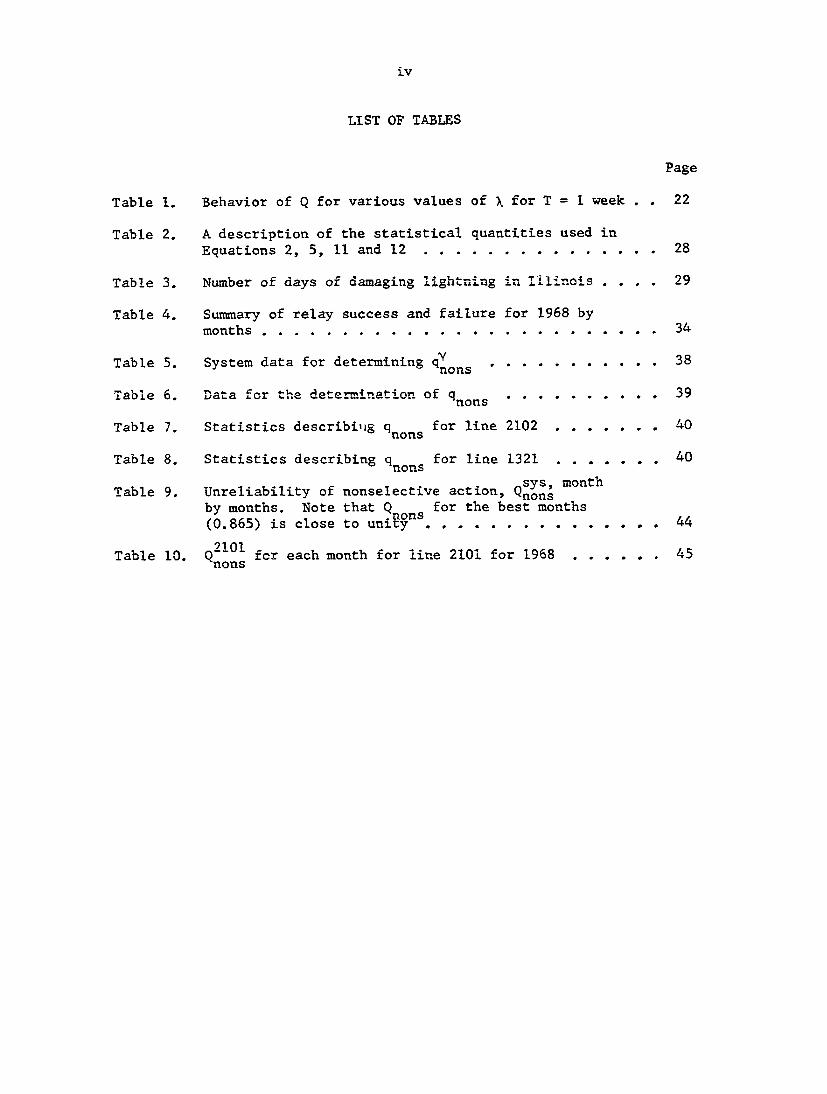
LIST OF TABLES
Page
Table 1. Behavior of Q for various values of X for T = 1 week . . 22
Table 2. A description of the statistical quantities used in Equations 2, 5, 11 and 12 28
Table 3. Number of days of damaging lightning in Illinois .... 29
Table 4. Summary of relay success and failure for 1968 by months 34
Table 5. System data for determining 38
Table 6. Data for the determination of q^^^^ 39
Table 7. Statistics describing line 2102 40
Table 8. Statistics describing q for line 1321 40 nons
Table 9. Unreliability of nonselective action, Q^ons by months. Note that Q for the best months (0.865) is close to uniSy"^ 44
Table 10. Q^"^~ for each month for line 2101 for 1968 45 nons

1
INTRODUCTION
Electric power companies have a substantial capital investment in
generating stations, transmission lines and distribution networks. To
protect this expensive equipment, protective relays are used to detect
the presence of faults (short circuits and other abnormal conditions)
which would damage the equipment or otherwise interfere with the normal
operation of the rest of the power system. These relays have a pair of
electrical contacts which close and energize an auxiliary relay to
handle the heavy currents necessary to operate circuit breakers. The
circuit breakers disconnect the faulted equipment thereby isolating it
from the rest of the power system.
As power systems grow in complexity, relays play a more and more
important role in the removal of faulted equipment. Since system
stability becomes more critical, relays are required to operate faster
and without errors. These requirements have resulted in relay manufacture
being characterized as an "art".
Relays operate by sensing voltages, currents ; phase angle and other
quantities which will enable them to distinguish a fault from normal
conditions on a particular piece of equipment. The normal state of the
relay is passive since faults are relatively rare. The relay is required
not to operate unless the fault which does occur, is on the particular
piece of equipment being protected. Figure 1 below is a one line diagram
of a section of a power system. The square boxes are circuit breakers,
the heavy lines are connection busses and the thin lines are transmission
lines. The dashed lines surround a section of transmission line to be

2
FAULT
foU-
Figure 1. One line diagram of a section of a power system
protected and indicate the "primary protection zone" for the relays on
either end of the line. Should a fault occur on line EF, two things must
happen.
1) The relays at each end of the faulted line (indicated by
arrows) sense this fault and open circuit breakers E and F.
2) The other relays such as are at A and B are expected to not
operate.
For this same fault on line EF, back-up relays are necessary to remove the
fault should a failure occur in the relays at E or F or in the circuit
breaker at E or F. These back-up relays are usually of the same type as
the primary relays and are enabled after a time delay long enough for the
primary system to normally isolate the fault.
The characteristic of relays which indicates their ability to
detect faults they were supposed to detect and to ignore other faults is
called selectivity. Selectivity may be gained by the use of particular
relays, by a particular configuration of relays and communication

3
channels or a combination of the two.
One of the first ways of providing selectivity as well as back-up
was through the use of a directional overcurrent relay with an inverse
time characteristic. This relay senses currents flowing in a certain
direction (down the line) above a preset magnitude. When the line
current exceeds this preset threshold, the relay responds with a time
delay inversely related to the magnitude of the current. For relays
closer to the fault, larger fault currents are seen and these relays
operate first providing selectivity. The more distant relays will
operate if the closer relays fail to isolate the fault, providing
natural back-up.
As relays were required to operate faster, instantaneous relays were
used for primary relaying, and with variable time delay for back-up
relaying. Two common types are instantaneous overcurrent and impedance
relays. Impedance relays make a continuous (analog) computation of the
complex ratio of voltage to current. The impedance seen by the relay is
the impedance of the transmission line plus the impedance of the load
connected to the far end. This quantity will be greater than the
impedance of the line alone unless a fault occurs on the line. These
relays are inherently directional.
For a fault close to the end of the line EF, as indicated in
Figure 1 a problem arises. How does the set of relays at F sense this
fault and yet not respond to a fault located on line AB near circuit
breaker B? Electrically, these two locations are very close to each
other. One solution is to set the relay at F to sense a fault along
as well as beyond the end of the line and provide a signal from the

4
other end of the line to block the operation of breaker F if the fault
is not on line EF. This blocking signal is present unless the relays
at E also sense a fault. This scheme is referred to as an overreaching-
blocking relay scheme.
The alternative to an overreaching-blocking scheme is an under-
reaching-permissive scheme. In this scheme if one of the relays senses
the fault, the related breaker is tripped and this trip is transferred
to all other circuit breakers connecting this line to the rest of the
power system.
The two schemes above detect the presence of faults based on "local"
information. Some relaying schemes in use utilize information from both
ends of the line. This differential protection requires a communication
channel for information as well as for transfer trip or blocking signals.
One of the major problems of reliable relay operation is the security
of the communications channels. These channels may be leased wire,
private wire, power line carrier current, public microwave or private
microwave. The security of the channels is part of a broader security
requirement to prevent spurious operations of any type.
The requirement of positive detection of all faults by the proper
relays and the prevention of unwanted trips is generally classed as a
reliability problem, or, stated another way, the probability of all
operations being correct. This "probability of correct operations" is
a definition in a wide sense. If a faulted line is cleared, either by
primary relaying or one of several back-up relays, and if there are no
spurious operations, the operations could be called correct. In this
thesis a more narrow definition will be adopted, one of fault-free
5
performance of the primary protection system vjhether it be a group of
relays protecting a certain transmission line or a digital system
protecting one or more transmission lines. Since we will compare the
reliability of existing equipment with that of a proposed digital system
the primary protection system will be defined to include:
1) primary zone relays
2) station batteries
3) mounting racks
4) interconnections between relays.
Specifically excluded are current and potential transformers,
circuit breakers and the circuit breaker trip mechanisms.
The purpose of this thesis is to derive two methods of calculating
the reliability of existing protective relays. These two techniques are
demonstrated by way of a numerical example. The numerical results are
discussed and compared with the reliability of a computer operated
protection system.

6
REVIEW OF THE LITERATURE
An extensive literature search was made in the area of power system
reliability. Many papers were found on the general topic of reliability
and many others on the problems of determining the reliability of power
systems. Most of the pertinent papers dealt with the prediction of
system reliability with respect to generator and line outages. Only
three papers, all published by Soviet authors (4, 11, 13) were related
to the topic of protective relay reliability. These papers were found
translated into English in Electric Technology U.S.S.R.
The paper by Smimov (11) presents the time independence of the
relay's inherent reliability and gives basic ground rules for determining
this reliability in a laboratory environment. He then discusses the
effect of field conditions on this reliability.
The paper by Fabrikant (4) presents the concept of the double
nature of relay reliability. The equations as stated in (4) are not
without errors. However, the approach adopted in the first portion of
this thesis is based on the concepts presented there.
The paper by Zul' and Kuliev (13) is useful in that they have
presented test data on a Soviet automatic protective device and have
shown that it follows the classical failure modes described by an
exponential time to failure.
A previous literature review brought to light several papers
(2, 5, 7, 9, 12) on computer operated substation protection systems.
All of the computer systems have basically the same hardware
requirements and the reliability of these systems is discussed in

7
this thesis.
À related paper by Corduan and Eddy (3) discusses three ways of
providing stored energy to isolate the hardware from power supply
perturbations. A reliable source of power is necessary for a computer
operated protection system.

8
RELIABILITY OF ANALOG RELAYS
Determination of the reliability of a protective relay or relaying
system is unique. The ordinary concept of probability of failure-free
operation does not directly apply. Instead, two reliability quantities
must be considered, q(x)^, the probability of a device failing to operate
properly in the presence of a fault it was set to detect and q(y), the
probability of a device operating in the presence of an external fault
which it is supposed to ignore (4). In addition, will refer to the
probability of a group of relays or relay systems failing to operate and
*'nons denote a group of relays or relay systems operating non-
selectively.
2 Assume that a fault outside the primary zone of the relay produces
unwanted trip signal, i.e., signals are produced when unnecessary. To
lower the probability of this nonselective action, we can place another
relay in parallel and connect them by a perfect logical AND element
(see Figure 2, case A). The probability of nonselective action is
ror the sake of brevity, this paper will use the notion of unreliability, q, which is related to the reliability, r, by the equation q = 1 - r.
so that
•nons is less than q(y)
2 The technique presented here applies equally well to a particular
device (a relay) or to a group of relays acting as a unit. Thus, relay and relay systems can usually be used synonymously.

Figure 2. Failure probabilities for different schemes
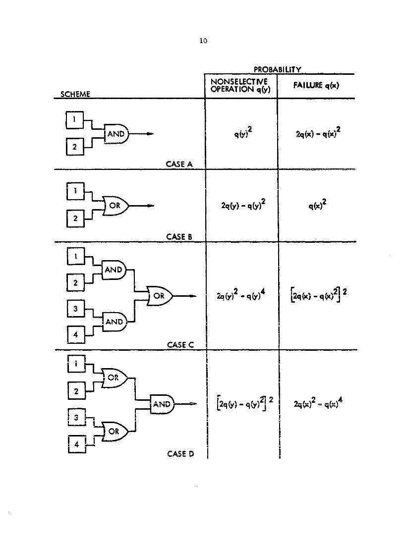
10
SCHEME
PROBABILITY
NONSELECTIVE OPERATION q(y) FAILURE q(x)
CASE A
q(y)^ 2q(x) - q(xf
2q(y) - q(y/
CASE B
: AND
2q(y)̂ -q(y)^
CASEC
{pqW - q^)^j ̂
[2q(y)-q(y)̂ ̂ | 2q(xr -
! 4
CASE D I

11
since q(y) is less than one.
However, this relay can also fail to operate in the presence of a
fault, i.e., no trip signal is produced when one is necessary. Connecting
two relays in parallel through the logical AND element results in a
probability of failure,
"fail = 1 - [i -
= 2q(x) - [q(x)]^
which is greater than q(x) since q(x) is less than one. Thus q^^^^ is
lowered at the expense of raising q^g^^'
For example, let q(x) = 0.05 and q(y) =0.1. If we connect two
relays with these characteristics together with a perfect AND element,
"nons "
= 0 . 1 ^
= 0 .01
which is a factor of ten improvement over each relay alone. However,
2 q^ail = 2q(x) - q(x)
= 2(0.05) - (0.05)^
= 0.10 — 0.0025
= 0.0975
which is worse than each relay alone by a factor of about two. This
example points up two things: 1) Both failure modes must be evaluated to
compare different schemes; 2) If q(x) and q(y) are very different (as
they may easily be), a trade-off is oossible between a and q^ to ' - nons fail

12
The scheme in case B of Figure 2, which is commonly used in power
systems, accomplishes opposite of case A, i.e., case B improves at
the expense of degrading The schemes of case C and case D improve
(lower) both q and q^ by using 4 relays and 3 logic elements, but ^nons fail
only if q(y) and q(x) are less than 0.382. If q(y) and q(x) are greater
than 0.382 it is not possible (4) to simultaneously improve and
a fact resulting from the double nature of the reliability of
protective relays. The practice of making a reliable system from
unreliable parts is applicable here only insofar as their inherent
reliability is sufficiently good.
If a relay fails so that the failure could lead to a failure of the
protection, this does not imply that a failure of the protection actually
takes place. For the protection to fail, the line also must be faulted.
Different from this is the nonselective failure where a trip signal
is sent for a fault external to the primary zone of the relay. Soviet
experience indicates (4) that almost all of the nonselective actions of
the relay occur simultaneously with an external fault. Very rarely does
the relay send a trip signal all by itself.

13
q, , — THE PROBABILITY OF A FAILURE TO OPERATE ^fail
With existing relaying systems, the relays do not operate unless a
fault occurs. Since faults are relatively rare, the relay spends nearly
all of its life in a passive state and doesn't see fault magnitude quanti
ties. This is all right, of course, because the relay needs to operate
only when a fault occurs. However, the problem is that one doesn't know
if the relay will operate correctly until the next fault occurs, at which
time the relay is called upon to operate. Thus the probability of
failure depends upon the frequency of faults occurring within the relays
primary protective zone. This is an inherent disadvantage. While the
relay is in its passive state, there is no way to predict whether or not
the relay will operate should a fault occur. A computer operated
protection scheme, on the other hand, has a probability of failure which
is less dependent upon the frequency of occurrence of faults on the line
and allows convenient prediction (via self-testing) of successful opera
tion should a fault occur.
For existing relay systems, the probability of a failure to operate
q^g^^ is dependent upon two quantities, q(x^) and q(x^). If x^
represents the event of a fault in the primary zone, then q(x_) represents
its probability of occurrence. Similarly, x^ represents the event of a
failure of the relay and its probability of occurrence is q(x^). The
probability of failure to operate of the relays on line y is given by the
intersection of the two events
sZail " 4(*a "S)
When the probability of one event is dependent on the occurrence of

14
another, a conditional probability is involved. The applicable relation
(10) for the intersection of two events in Equation 1 is
Sfail = q(Xa)4(=bl=a)
The probability q(x^|x^) does not equal q(x^) unless the events are
independent. For existing relaying systems, events x^ and x^ are not
independent, and Equation 2 cannot be simplified. For existing relays, we
may define the probability of a failure in the relay as a function of
the number of operations the relay performs. Of course, the number of
operations in a year depends upon q(x^), the probability of faults on the
protected line in a year. On the average, the relay will fail on a
certain percentage of the total number of operations.
It is common practice in reliability work to use time (or a time
period T) as a basic index instead of the number of operations. Due to
this use of time as the basic index, a relay placed in service on a line
with greater fault-proneness (faultability) will exhibit a shorter
average (mean) time between failures (MTBF) than a similar relay
placed in service on a less fault-prone line. This change in MTBF
isn't due to any inherent change in the reliability of the relay, but
instead is due to the choice of HTBF as the index of performance.
Note that MTBF is an excellent index to use for the reliability of
a digital computer as the failures are indeed time independent. We
should also note that a common index is necessary to compare the re
liability of the two systems. Hence, we shall use the unreliability
based on MTBF to measure both systems in order to make a comparison of
the relative reliability of each.

15
The ratio of the number of faults internal to the number of faults
external to the primary zone of the relay can be related to a "level of
exploitation" (11) of the relay. The inherent reliability of the relay
itself is independent of its placement^ but the probability of a given
relay operating successfully for a time T depends on the faultability
of the line as well. Suppose we have a relay that fails to operate three
per cent of the time, q(x^lx^) = 0.03. If placed on a line with
100 faults/yr, the mean-time-between-failures (MTBF) is 365/3 or 122
days. If this same relay is placed on a line with 200 faults per year,
the MTBF is 61 days. For a given period of time, if a relay sees more
faults, it will fail more often since q(x^|x^) is a statistical parameter
which is a constant for each relay. In summary, we note two things:
1) the probability of successful operation (reliability) is
dependent on the faultability of line, since r = 1 -
2) The use of time as a base, i.e., MTBF, is not completely
satisfactory for existing protection relay systems.

16
G — THE PROBABILITY OF NONSELECTIVE ACTION ^ons
There are two ways a relay can act nonselectively. First, the
relay may act in a nonfault condition. This may be due to a slow
failure of the device such as from age or environment or due to a dis
turbance of the relay. Second, the relay may act due to a fault
occurring outside its primary zone (an external fault) simultaneously
with a relay failure. Soviet experience (4) shows that most nonselective
actions of relay protection systems occur in conjunction with external
faults. Based on operating data presented later this is not true for
U.S. power systems, where most nonselective acts are caused by security
failures.
Referring to Figure 1, the relays at A or B should not operate for
a fault on line EF. If they do operate, it is a nonselective operation.
The probability of this type of failure is
AB / AB. ^ / EF. , AB| EF. Snons = Stfs > + 'ra >
where q(y^) is the probability of a nonselective operation due to a
EF security failure on line AB, qCy^ ) is the probability cf 2 fault on
line EF and q(y^^|y^^) is the probability of the relays on line AB
responding to the fault on line EF when it occurs. In general, let
q(yj) equal the probability of nonselective action occurring on line y
when there are no external faults.^ If y^ represents the event of a
^This should include nonselective operations due, for example, to a workman drilling on the relay panel as well as other nonfault related events.

17
fault, external to line y then the probability of external faults on
lines 2, 3, , m equals qCy^), q(y^), , q(y^. Let the probability
of a relay on line v failing so as to act nonselectively in the presence
of external faults (a conditional probability) equal q(y^|y^),
q(y^|yg), , ̂ iCy^ly™)- The probability of nonselective operations on
line Y is the product of the probability of no security failures and the
probabilities of no fault related failures. Stated mathematically for
line Y,
<ons = 1 - q(ya)q(y2!ya)]
[i - q(ya)q(yy ly^)]. (3)
If q is 0.1 or less, we can use an approximation for a small loss ^nons
in precision.
sZoas + q(ya)q(y%|ya) + + q(ya)q(yt)ya). (4)
Then for line y,
N
Snons = + E ^ m=l
#Y

18
COST OF RELAY PROTECTION
From the above it is clear that the probability of nonselective
action, well as the probability of failure to act, are
dependent on the faultability of the lines they are protecting as well as
the relay's inherent reliability. Due to these dependencies, one car.iot
simply add q^^^^ and q^^,^ together to obtain a composite unreliability
because the costs associated with nonselective action and failure to
act usually differ. Stated mathematically, using C to indicate the
relative cost per operation,
cost = Cf,;! qgaii + (6)
Naturally the best type of back-up protection then is that which
reduces both q_ and q . The cost is then reduced independently of fail ^nons
the values of the individual quantities. It can also be seen that adding
an identical parallel protection system may or may not improve the
protection, since both q and q_ .. are affected. nons fail
Operating data for a given protection may indicate that q^^^^ =0.1
and q, =0.01. If Cr and C are known or can at least be ^fail fail nons
approximated, then Equation 6 above will give the cost per operation.
If two cf these systems are connected together with a perfect logical
AND element, q will decrease, q ^ will increase and the cost may go nons
up or down depending on the relative magnitudes of C^^^g and
Thus, it is possible to evaluate different schemes and to make a decision
as to which one is better (from the standpoint of lower costs).

19
APPLYING CLASSICAL RELIABILITY THEORY
Classical reliability theory is often concerned with random failures
described by an exponential density function, f(t) similar to Figure 3
except for the scale factor 1/X.
f(t) = Y ̂ ̂
The distribution of failures is given by F(t).
F(t) = / f e'^^dx = r' 1 J o k
F(t) = 1 - e'^-
where x is a dummy variable. Since the integral of f(t) from t = 0 -»»
is unity, the probability of one or more failures from t = 0 -* T is given
by ^
Q(T) = f(t)dt
Q(T) = 1 - e"^^
The probability of success R is related by R = 1 - Q, so
R(T) = e'^^.
Figura 3 sho%s hcv R(T) varies as a function of XT. If the failure rate
X is constant then the equation for R(T) above will also give the
probability of success for any time interval, T.
There are usually three distinct types of failures. Early in the
lifetime of a device,^ failures are often due to initial weakness or
defects, weak parts, bad assembly, etc. During the middle period of
device operation fewer failures take place^and the failure rate, X, is
1
^Here again, device may indicate a relay or a group of relays acting as a unit.

20
1.0
0.8
0.4 0.2
0 0.1 2
XT
Figure 3. Reliability for an exponential density function
constant with respect to time. (For relays, X is constant with respect
to the number of operations.) Since the cause of these failures is
difficult to determine, these middle-life failures are characterized
as random events. As the device wears out, the failure rate, X,
increases again. In a well-designed and tested relay, the burn-in phase
may be small or even nonexistent. We will make the usual assumption that
our data reflects devices which are all in ths normal, =iddle-life
phase where failures are random and their failure rates (X*s) are
constant.
Figure 4 shows the results from Soviet tests (13) on an automatic
reclosing device. The vertical axis indicates the failure rate per
operation. The horizontal axis indicates the number of operations. The
burn-in, middle, and wearout phases are easily recognized and are denoted
by I, II and III respectively. This curve follows the general "bathtub"
curve which is so well known in reliability theory (10).

21
X
NUMBER OF OPERATIONS
Figure 4. Failure rate of an automatic reclosing device as a function of the number of operations
The reliability of a device which meets the stated conditions is
given by
R = e"^^ (7)
where X is the failure rate or the number of failures per unit time during
the middle life and T is the time period involved. R stands the
probability of success (no failures) for the time period T. The un
reliability or probability of failure is given by
Q = 1 - e"^^ (8)
where X and T are as defined above and Q is the probability of one or
more failures during the time period T.
An example is in order. Let us pick a time period such as T = 1
week. By selecting various values for X» we can see the behavior of Q,
in Equation 8, summarized below in Table 1.

22
Table 1. Behavior of Q for various values of X for T = 1 week
Q X(Failures per week) MTBF = Y
0 0 CO
0.01 0.010 100 weeks
0.095 0.10 10 weeks
0.393 0.50 2 weeks
0.632 1.0 1 week
0.99965 10.0 0.1 week
As we can see from Table 1, the probability of a failure in a one
week period, Q, is about 10% when there is an average of one failure per
10 weeks (MTBF = 10). This example demonstrates a very important
property of Equation 8. In order to obtain a meaningful measure of the
probability of failure it is imperative that Q be specified for a
specific time period and the appropriate X used for that time period.
When using Equation 8 to determine the probability of failure during long
time periods, a difficulty arises. It is assumed that the events giving
rise to the failures described are randomly distributed with respect to
time (during the time period T). If the time period is long, the failure
rate may vary during the time period. However, X can be assumed constant
over some set of shorter time periods which make up the longer time
period. In this case the X in Equation 8 represents the arithmetic mean

23
of the X's which described the failure rates over this set of shorter
time periods. To say it another way. Equation 8 assumes X is constant
over the time period T. When Equation 8 is applied to protective relaying
reliability the failure rate \ is anything but constant when a period of
one year is involved.
Rather than use Equation 8 as is, let us assume that X remains
constant only during each month of the year and develop the appropriate
expressions to be used later. Let represent the failure rate for one
month. Then the probability of no failures for January, Rj, is given by
where T^ = one month. Similarly, the reliability R^ for any month i is
given by
R. . C9)
The probability of no failures for January through December is
I one year R. _ _ = f] R^ i = 1,2,...,12
1 - X/I»
= 1 [ e ^ i = 1, 2 , . . . , 12 i
. . . 4 - \ g ) T = e u. 2 J i-
rearranging.
-(X-]_+X2'^X3 + ••• + X^2)
R =6 one year 12
Also,
- (Xi +X9+X-, • • • + Xi?)
year = ^ ' 12 —

24
Comparing the right side of Equation 10 with Equation 8 above, we can see
that
which is the arithmetic mean of the monthly failure rates. The simple
relation of Equation 10 enables one to derive yearly reliability quantities
from statistics compiled monthly. It is important to note that there is
likely to be a large variance associated with the monthly given by
Equation 9. Equation 10 represents an "averaging" of the monthly data.
This is due to the nature of the application of classical reliability
theory to power system protection.
Since there are two failure modes present, failure to operate and
nonselective operation, there are two applicable expressions for R
(or Q), one for each of the failure modes. That is. Equation 8 above
gives rise to two equationsr
12T^=XY
or a period of one year and that
X = 12
fail T
(11)
-À T nons
(12) ^nons
In general, Q and will be different because they arise from ° ' nons fail
two failure modes.

25
PREDICTION OF PROTECTIVE RELIABILITY
The typical reliability problem concerns a system which is activated
and performs its task until it fails. The system does not operate again
until it is repaired. Furthermore, it is usually easy to tell when the
system has failed since the output ceases (e.g. a communications systems).
A protective relaying system is "activated" when a fault or line
disturbance occurs. The normal state of a relay can be assumed passive
since the effects of age and environment are usually minimized by careful
design.
Due to the extremely short period of operation it is not possible
to even consider repair of the relay at the time of failure. For this
and other reasons, some form of back-up (standby) protection is required.
Since the back-up relays are also unreliable, we should provide back-up
protection for the back-up relays, and so forth. Even if infinite funds
were available, it will not be possible to reduce the probabilities of
failure to zero. This is a direct result of the interconnection complexity
encountered in implementing N back-up schemes. These N schemes must be
connected together with logical elements (as in Figure 2) which are not
failure free. If for no other reason, a graph of the costs (see Equation
6) associated with the probabilities of failure as a function of the
number of back-up schemes, N, will exhibit a definite minimum.
A typical approach to the prediction of reliability has been to
describe the probability of success in terms of the probabilities of
success of the individual components. The procedure is to describe in
closed form, by using logic equations, all of the possible combinations

26
for success (or failure) of the system and their probabilities. This
technique has been proposed for protective relaying systems (11), however,
the technique has several practical drawbacks. 1) Due to the complexity
of modern relaying systems the logic equations become difficult to
V V formulate. 2) Calculation of q, .. and q by combinational methods is
xsii. Hons
not possible since the individual q(x^|x^) and q(y^ly™) for each relay
are not generally known.^
The approach adopted here is to apply both the conventional
description of Equations 2 and 5 and the classical description given by-
Equations 11 and 12. A subtle but important difference exists between
the two techniques for evaluating relay performance. The description
given by Equations 2 and 5, repeated below,
sins " 9(y%) +%] q(yT)q(yZ'yT) (s) m=i o a
is the probability of failure of the set of relays on line v each time a
fault or nonselective operation occurs on the payer system^ This
description meshes quite well with several intuitive descriptions
currently being used by electric utilities to characterize relay per
formance. Using Equations 2 and 5 and the appropriate data, the
probabilities of failure given a fault has occurred, q(x^lx^) and
"Values of q(xblxa) and q(yg!y^) seem to be unknown even by US relay manufacturers. The implication is that the appropriate statistics would have to be determined in the lab, which is not a pleasant prospect.

27
q(y^|y®), can be calculated for each set of relays in addition to
qt . and qj . Since q(x, J x ) and q(yj|y°^) are independent of time and liâxL lions , D 3 D â
geographical placement of. the relays.and represent the probabilities of
failure of each relay system acting as a unit, they are extremely useful
quantities for comparison of different relaying schemes.
In contrast, the unreliabilities given in Equations 11 and 12,
repeated below,
Qfail = 1 - e"^ fail^ (11)
X X O = 1 - e nons (12) ^nons
represent the probabilities of one or more failures in the time period T.
The time period T can be interpreted as the time between routine maintenance
checks. This interpretation of T doesn't suit relays very well because
they spend most of their life in the passive state and it is difficult if
not impossible to determine a priori if the relays will fail the next
time a fault or spurious signal occurs.
If we think in terms of a substation computer operated protection
system, however, the concept of routine maintenance and the ability to
predict the future success of fault detection are very relevant. At
this point it is anticipated that the and of a computer
operated protection system will be so low that other previously neglected
contributors to unreliability will now dominate the protection system
unreliability.
Depending on how Equations 11 and 12 are used in conjunction with
the protective system operating data, four pair of Q's can be calculated:
1) and for all the relays on the power system for

28
each month.
2) and for all the relays on the power system "averaged"^
for the year.
3) Qggii *^ons each set of line relays acting as a un.it
for each month.
4) Qc -1 and Q for each set of line relays acting as a unit fail ^nons •' °
"averaged" for the year.
The statistical quantities in Equations 2, 5, 11, 12 are enumerated
in Table 2 below.
Table 2. A description of the statistical quantities used in Equations 2, 5, 11 and 12.
Quantity Description
^fail
Y nons
q(yj)
KYbiy:)
Number of failures to act in the presence of a fault per time period.
Number of nonselective actions due to security failures or external faults per time period.
The probability of a security failure occurring on line y.
The probability of a fault on the system occurring on line y.
The probability that the line relays will fail to act given the fault, x^.
The probabilities of a fault occurring on line m.
The probabilities of the line relays on line V operating nonselectively given that a fault has occurred on line m.
1 See Equation 10.

29
To summarize, the predictive approach adopted here is to characterize
mathematically the two failure mechanisms using two different descriptions.
Then, one can interpret (untangle) the operating statistics and calculate
useful reliability indexes with which to judge and compare the per
formance of line relays and of the protective system as a whole.
Variation of \ with Respect to Time
Let us digress for a moment and investigate the expected variation
of both \'s with respect to time. Since a numerical exançle later in
this thesis uses data from a major Illinois electric utility it is
appropriate to discuss the incidence of lightning in Illinois.
By coincidence, an excellent paper exists (1) specifically concerned
with the incidence of damaging lightning in Illinois for the period
1914-1947. All the remarks herein jrefer to conditions only in Illinois.
Table 3 below shows the number of days of damaging lightning by months.
Table 3. Number of days of damaging lightning in Illinois
Month Total # of days Fraction of total
January 2 .0043 February 8 .0173 March 17 .0367 April 20 .043 May 45 .097 June 94 .203 July 114 .246 August 108 .233 September 36 .0777 October 17 .0367 November 2 .0043 December 0 0
TOTAL 463

30
As expected, the peak of activity occurs in the summer months. Over
2/3 of the days experiencing damaging lightning occur during June, July
and August. In the May 1 - September 15 period, 80% of all days with
damaging lightning occurred.
The two months with the highest lightning frequency are July and
August, while the months with the greatest number of thunderstorm days
are May and June. No solid reason exists to explain this disagreement
between two such highly correlated weather phenomena. One of several
possible explanations (1) is simply that thunderstorms occurring in May
and June do not produce as many or as strong cloud-to-ground discharges
as they do in July and August. It is also interesting to note that the
maximum number of occurrences of lightning during the day was found in
the early afternoon between 1 p.m. and 4 p.m., local time.
The year to year variance in the data of Table 3 can be summarized
by noting that the maximum number of days per year was 34 and the average
number was about 14.
It is reasonable to expect the failure rates of Equations 11 or 12
to vary as a function of the fraction of the total number of days in a
given month divided by the total number for the years. For example,
X- , ~ 114/463 = 0.246 juxy
Figure 5 indicates the expected variation of both X _ and X on a ° fail nons
relative basis. Since Figure 5 represents a 34 year period, we can make
3 judgment as to whether or not the year being studied is normal by
comparing the observed variations in the X's with Figure 5. One should
note that the shape of Figure 5 will vary with geographical location.
It also must be recognized that lightning is not the sole cause of

31
X
Ùiiwilf^^ I I t I I 1 L_3& J F M A M J J A S O N
MONTH
Figure 5. Expected variation of the failure rates by months due to
relay failures. Human errors and communication channel failures are
important statistically especially in the winter months when severe
weather is relatively rare. Other fault related events include, for
example, airplanes hitting the lines and squirrels climbing in the
switchgear. However, lightning (or weather in general) is something we
have no control over and will always be with us. If one reduces failures
due to human errors, for example, this will in turn change the graph of
the variation of X by months snalagous to Figure 5. If one reduces all
causes of failures except weather to zero, then, in the limit, the graph
should approach the shape of Figure 5. Data presented later will
indicate the variation of X for a one year period.
lightning

32
A NUMERICAL EXAMPLE
The main objective of this numerical example is to provide a clear
path from the analytical results to their application to actual operating
data. In short, the main results represented by Equations 2, 5, 11 and 12
are applied to the determination of q_^_g, Qfgii '^nons
specific power system transmission line relays. Given a sufficient
quantity of operating data (many years worth) one can calculate the
various q*s and Q's mentioned above. The results based on one year's
data are not all expected to have a high confidence level due to the
limited number of data points relative to the variance of the data.
Exhaustive operating data were obtained from Commonwealth Edison
Company (CECo) for the year 1968. CECo serves approximately the northern
one third of Illinois including Chicago and has one of the highest peak
loads in the United States. The territory served experiences a wide range
of weather conditions typical of the North Central United States.
The operating data usedvere derived from daily company reports and
concerned 128 transmission lines operated at 138W and higher. Lower
voltage equipment was included when it was connected directly to the
higher voltage without a circuit breaker. The relays used for protecting
lines of 138kV and higher are roughly comparable and are generally of the
latest design. Various schemes are used and include permissive, blocking,
differential comparison and phase comparison. Most of the lines have a
transfer trip (TT) capability using public and private communication
channels. TT refers to the requirement of the first relay which responds
to the disturbance to trip all of the circuit breakers connected to the

33
line.
Since the TT relay is only an auxiliary relay and does not respond
to the disturbance directly, it is not included in the reliability
statistics. Also excluded are generator, transformer and bus faults.
These faults are detected by their own sets of relays and are beyond
the scope of this example, but they could be evaluated by the same
technique.
Each reported disturbance was noted with regard to the following
criteria:
1) The nature of the disturbance
a) Caused by a short circuit in primary relaying zone
b) Caused by a short circuit outside primary relaying zone
2) Weather related
3) Occurrence of nonselective action
a) Fault related
b) Security failure (i.e. spurious trip signal)
4) Occurrence of failure to operate.
The analyzed data are summarized in Table 4. A great deal of care
was taken to exclude redundant information from the raw data. In each of
the 306 disturbances a set of transmission line relays responded to what
appeared to that device to be a fault. There were a total of 133 actual
faults involved in the 306 disturbances. Table 4 shows that a majority of
the line disturbances ('^0%) are not weather related, and we will assume
that these are randomly distributed throughout the year.
Of the 306 disturbances considered, only about 40% were weather
related, and all of these except for December and part of January were

34
Table 4. Summary of relay success and failure for 1968 by months
Line Weather ^fail X nons
X nons
Due
Relay Related Failure Nonselective Month Operations Operations To Operate Operations Fault Ott
Jan. 25 10 0 5 5 0 Feb. 4 0 0 2 0 2 March 12 6 0 2 0 2 April 20 9 0 8 5 3 May 25 8 0 8 3 5 June 34 25 0 2 1 1 July 35 8 0 15 1 14 Aug. 67 47 0 13 7 6 Sept. 20 6 0 6 2 4 Oct. 7 1 0 4 2 2 Nov. 16 0 0 9 2 7 Dec. 41 18 0 9 4 5
Totals 306 136 0 83 32 51
caused by lightning. The corresponding weather related failures due to
lightning are plotted in Figure 6 (curve 1) along with the data from
Table 3 (curve 2).
O CURVE 1 ® CURVE 2
MONTH
Figure 6. Comparison of 1968 weather related disturbances (curve 1) with the 34 year average incidence of lightning (curve 2)

35
We can see from Figure 6 the expected correlation between the weather
related disturbances due to lightning for 1968 and the incidence of
damaging lightning given in Table 3.
Determination of from Operating Data
"/ail " •'a'
The event is the occurrence of a fault on line y and is a
failure to respond to that fault by the set of relays protecting line y
A useful quantity which is independent of relay placement is q(x^|x^).
Since it represents the probability of failure given a fault, q(x^|x^)
is useful for comparisons of different relaying schemes. For line y,
. _ number of failures of the relays on line y_ a number of faults on line y
Note that the denominator is not the total number of operations for line
Y, because this would include operations due to security failures. If
the relays do not respond to a spurious trip signal, for example, there
no loss of reliability.
The probability of occurrence of a fault x_ is denoted by q(x^).
For line y
. . _ numu-r of faults on line Y a number of faults on all lines
Therefore, there are two useful quantities related to the "good
ness" of the relays with respect to failures to operate on line
Y — and q(x^Ix^). In order to realize the best return for each
dollar spent on protection (with respect to failures to operate) it is
desirable to make all the qY for each line equal to each other. This ^fail ^
is called the constant hazard aonroach (10). This aooroach implies the

36
use of more reliable relays on more fault-prone lines to obtain a constant
different protection systems independent of location. Alternatively,
q(x^l x^) is the inherent unreliability of the relay.
If we assume that a computer operated protection system would be
more reliable than the relay system it would replace, then the line or
lines with the highest faultability, q(x^), represent the best placement
of such a system for maximum improvement of reliability with respect to
failures to operate.
As shown in Table 4, there were no failures to operate in the
presence of a fault on the CECo system for 1968. As a result all
for all lines are identically zero. Also, q(x^Ix^) equals zero for those
lines on which faults occurred. No data is available for 1968 to deter
mine whether or not q(x^lx^) is zero for the lines which were not faulted.
Assume a fictitious failure to operate on line 0000 out of 6 total faults
on this line. Then, for the relays protecting line 0000,
The other quantity is q(x^]x^) and is useful for comparing
0000 "^fail
1/133 for 1968.
Determination of q^ from Operating Data
The event y^ is a nunselective operation on line V due to a security
failure and q(y^ is its probability. The event y^ is an external fault
V on line m and y^' is a nonselective operation on line V due to the fault

37
on line m. If there are N lines, then for small
Cns - + E nF=l Tn^y
as in Equation 5.
The quantity q^^^^ is the probability that the relays protecting
line Y will operate nonselectively when either a security failure or a
Y fault external to line Y occurs. The quantity q has two aspects.
•' ^nons
The first term on the right side of Equation 13 above is not fault
related and is due to security failures. For line y,
X Y\ _ nonselective operations due to security failures on line Y s total number of nonselective operations on system
(14)
The summation term in Equation 13 contains probabilities concerning the
other N-1 lines in the system. For line m, mfY,
/ _ number of faults on line m r. Number of faults on system
Also, for line m,
- Y| ni _ nonselective operations on line Y due to faults on line ^b number of faults on line m
m
(15)
V To compute q^^^g in general requires one application of Equation 14 and
N-1 applications of Equations 15 and 16. In practice, virtually all
nonselective operations will be due to security failures as well as
faults on adjacent lines, thereby reducing the number of computations
from the general case. Since the quantities of Equations 15 and 16
always occur in product form in the summation of Equation 13, one could
take advantage of che cancellation between the numerator of Equation 15

38
and the denominator of Equation 16. However, the identity of the two
quantities will be lost, and q(y^!y°) is useful.
Let us compute two lines representing both types of
nonselective operations. The necessary system data is listed in Table 5.
Y Table 5. System data for determining q^^^^
Number of faults Number of nonselective on the system operations on the system
133 83
Line number 2102 operates at 345 KV in central Illinois and is
interesting in that all of the nonselective failures were due to security
failures and none were due to the 7 adjacent faults. Line 2102 had 6
nonselective operations during the year, all due to spurious microwave
transfer trip signals. Using Equation 13 above and Table 5,
W = + lis (0) + ill + lis + 153 (°) - 0:07 <">
This is an appropriate time to note the large variance associated
with the use of Equation 13 and the result of Equation 17 due to the
small sample space. Several years data for line 2102 must be incorporated
into Equation 13 in order to have a high confidence in computations such
as 17.
Line number 1321 operates at 138 KV in central Chicago and is
interesting because none of the nonselective operations were the result

39
of security failures and all occurred simultaneously with faults on
adjacent lines.
Table 6. Data for the determination of q ^nons
Number of faults Nonselective operations of line 1321 Line m for the year due to faults on line m
1323 2 2
1210 1 1
Using Equation 13 and Tables 5 and 6,
w - ° + A
W = 0-02
y A listing of q for all N lines will indicate which of the lines
^nons
have more unreliable relays^ For these lines, more insight into the nature
the unreliability and what can be done to improve it can be obtained from
a look at q(yJ) and q(yj^jy™). Table 7 below lists the appropriate
statistics for line 2102, and Table 8 below lists similar data for line
1321.
From Tables 7 and 8, and Equations 13, 14, and 16 one can conclude:
1) Line 2102 is less reliable with respect to nonselective
2102 1321 operations because a > a
"nons "nons
2) All of the nonselective operations on line 2102 are due to
2102 y security failures because qrions ~ q (y^ ) for line 2102.

40
Table 7. Statistics describing q for line 2102 ^ons
1̂ "= q̂ ons 9(7̂ ) q(yj)
2102 0.072 6/83 2101 3/133 0 2105 2/133 0 11608 1/133 0 8014 1/133 0
Table 8. Statistics describing for line 1321
Line W stTs)
1321 0.02 0/83 1323 2/133 1 1210 1/133 1
3) All of the nonselective operations on line 1321 are due to
adjacent faults because q(yj) = 0 for line 1321.
4) Line 2102 is not affected by adjacent faults, but the reliability
of the line relays could be improved by increasing the security.
5) The security of line 1321 is fine, but the line relays operate
every time there is a fault on lines 1323 and 1210 since
= 1 for all faults on those two lines.
Lines 2102 and 1321 were selected for this exszple as s vehicle for

41
explaining the necessary calculations to determine q% and and ^ ^ ^fail nons
actually are less reliable than the average transmission line on the
CECo system.
Determination of Q^gj^l Operating Data
From the operating data regarding failures to act, CECo appears to
have nearly solved this portion of the reliability problem. There were
only two failures to act during 1968. These failures were due to a
communications channel failure and a wiring error, neither of which are
fault related. Consequently, ^ 0 for the year since the relays
never failed to act in the presence of a fault. The unreliability
Qfaii, for each set of line relays and for the protection system as a
whole for each month and for the year are all equal to zeîfo since there
were no failures to act, i.e. = 0 for 1968.
In order to see how a nonzero failure rate will affect the various
quantities numerically, we will assume a fictitious failure on
line 0000 in June. For the system for the year, since = 1 in
Equation 11,
-1 - e-i tail
4:1
For the system for each month i,
QÎYÎ; ^ = 0; i # June 1.CSX J.
and q!?:; J"»® = 1 . fail
sys June , n.632 fail

42
Looking next at the for each set of line relays on the system,
for all sets of relays equals zero for the year and each month
except those on line 0000. For the relays on line 0000 for the year,
,0000. yr.,. ,-l
= 0.632
For line 0000 for each month i,
^0000, 1 . 0 i f June
0000. June , ̂ s,, fail
Since the existence of one failure has such a dramatic effect on
the unreliability a word of explanation is in order. In the
typical application of classical reliability theory, one is usually
interested in the probability of mission success where the length of
time involved in the mission is much less than the MTBF (reciprocal
of the failure rate). This implies that Q is near zero, or the mission
is no-go. In protective relaying systems, it is common for many failures
to occur (both failures to operate and nonselective operations) in a
one-year period. As a result, the unreliabilities describing the
performance of the relays are often close to unity. The fact that the
unreliabilities are close to unity simply shows that the probability of
a failure in a one-year or one-month period is very large. The analysis
of protection system reliability in terms of classical reliability theory
is useful, however, in order to compare existing performance with the
performance of a computer operated protection scheme.

43
Determination of 0 from Operating Data ^ons
The more severe reliability problem is obviously the existence of
84 nonselective relay operations. It is obvious, but important to note
that there is no protection system provision for back-up to protect
against nonselective actions. In fact, the disproportionately large
number of nonselective failures is a direct result of overkill in the use
of parallel redundancy to lower the probability of failure (see Figure 2,
Case B). The conclusion then is to use less not more parallel redundancy
to obtain a lower cost of protection, as indicated in Equation 6.
Of direct value to the determination of is a graph showing
the variation of the failure rate due to all nonselective actions. The
nonselective actions are further divided into two subclasses — fault
related and nonfault related (security failures). A statistically
significant number of the security failures in 1968 were due to spurious
transfer trip signals on common carrier microwave channels (17 for the
year, 12 in July alone). Note the large difference in the two curves of
Figure 7 for July. Figure 7 shows the total numb^er of failures for each
month due to nonselective actions as well as the nonselective failures
due only to faults occurring on other lines.
o ALL NONSELECTIVE FAILURES e WEATHER RELATED NONSELECTIVE FAILURES
nons
MONTH Figure 7. Variation of by months for CECo - 1968

44
The number of nonselective actions for each month and the associated
•nons from Equation 12 is given in Table 7 below.
Table 9. Unreliability of nonselective action, months. Note that for the best months (0.§§§f is close to unity
^ _sys Month nons Q
nons
January 5 0. ,993 February 2 0. ,865 March 2 0. ,865 April 8 0. ,9993 May 8 0. ,9993 June 2 0. .865 July 16 ~1. ,0
August 13 ~1. ,0 September 6 0. ,9975 October 4 0. ,98 November 9 0. .9998 December S 0. .9998
Q^ons the year is also given by Equation 12
X T qyear = i _ ^ sons nons
- -84 = 1 - e
qyear = i _ IO-34 nons
(18)
One can also determine the Q for each set of line relays. It ^nons
is necessary to enumerate the line number and the number of nonselective
actions for that line (X ) then apply Equation 12 again. nons rir J -L o
For example, let us calculate for line 2102. This line is
about 150 miles long, operates at 345 KV and runs north-south through

45
central Illinois. Table 10 below shows the calculated values for Q nons
by months for this line.
Table 10. for each month for line 2101 for 1968 ^ons
Month ^ 2101 .2101 nons nons
January 0 0 February 0 0 March 0 0 April 0 0 May 0 0 June 1 0 July 1 0 August 0 0 September 0 0 October 0 0 November 0 0 December 0 0
For the one-year period of 1968, the "average" unreliability for line
2101 is
Qaons = 0-3*5 (1*)
In other words the probability of at least one nonselective operation on
line 2101 during the year is 0.865. Similar calculations could be carried
out for each line.
The calculations implied for each set of line relays for each month
and for the year will soon become tedious. There must be a lonely

46
computer somewhere to do these calculations painlessly to 10 nonsignificant
figures. Since the data from many years must be crunched, some standard
format for data entry and a program to process the data seems prudent.

47
COMPUTER OPERATED PROTECTION RELIABILITY
Digital computers and related equipment used in substations to
perform protective relaying functions offer zany advantages over con
ventional relaying systems. The flexibility offered by the computer
system hardware and software (6) allows one to greatly improve the
reliability of the protection system.
As before, the probability of a failure to operate is
Ifail ° "P
However, for a digital system, the probability of a failure to operate
given that a fault has occurred, q(x̂ |x̂ ), is independent of q(x̂ ).
Therefore we have
q^Lii " 9(^9(V CO)
where q(Xy) represents the probability of failure of the digital system
and q(Xg) is the probability of a fault.
As before, the probability of nonselective operation is
Since the digital system design can anticipate transients and system
swings due to adjacent faults (5), the summation tern above may be
assumed to be zero. Any nonselective operations which occur as a result
of faults can then be characterized as security failures and included in
V q(yg/. Therefore we have
Ws " (21)
Y where qXy^) represents the probability of a nonselective operation of

48
the digital system due to security failures.
A failure in the digital system can occur either as a hardware
failure or as a software failure. The reliability of small process
control computers is very good. The MTBF of the central processor and
the memory is about 8000 hours (one year = 8760 hours). The probability
of a hardware failure is given by classical reliability theory in
Equation 8.
Q = 1 -
For digital systems, the a priori probability of a hardware failure can
be predicted for a time period T based on the time interval between
routine maintenance. By expending a sufficient amount of time and
money for maintenance the probability of a hardware failure can be made
arbitrarily low — an option not available in conventional relaying
systems. For the probability of one or more failures for a year period
on line y due to hardware failure.
V
^failj hdwe = qCXg) ] (22)
where T is the interval between maintenance checks and >. = 1/8000 hours.
y It is obvious from Equation 22 that hdwe made quite small.
Similarly, a hardware failure could cause nonselective operations.
Other contributors to the nonselective unreliability are communication
channels and other security failures. One can write for a one year
period
-n'y = g/ ̂/I Sons, hdwe ' 's^ X + (1 - e ) (23)

49
where y and T are defined as in Equation 22 above and q(y^ represents
the probability of a nonselective operation due to security failures. The
amount that q(yg) contributes to Equation 23 depends very much on the
protection system philosophy and subsequently on the seriousness of a
y communication channel failure. For example, hdwe be greatly
improved if
1) Schemes requiring communication channels for information and
transfer tripping are not used
2) An oveireaching-blocking scheme ̂ used based on local
information.
A transfer tripping scheme is interconnected by a multiple input OR
element (the TT auxiliary relay) which is unreliable. Compounding this
is the lack of reliability demonstrated by some of the TT coEisunicatiori
channels. An overreaching- (responds to faults beyond the end of the
line) blocking (blocks a line trip of the fault isn't between the sets
of relays) scheme has the dual advantage of providing positive detection
of line faults and of graceful degradation should a communications failure
occur, \ Consequently this system will exhibit a lower Q nons
These improvements do not come without cost however; the price is an
increase in 0- Similar to Equation 6 regarding the cost of 'raix, nawe -
protection per operation, we have Equation 24 below relating the un
reliability to protection costs for a time period of one year.
^°®%ear ̂ ̂ fail'^fail ̂ ̂nons^ons
Based on past relay performance, a trade-off between and
would be desirable and economically justifiable.

50
If the computer software is written properly and debugged (no
small task), the unreliability due to a software failure will be zero.
Once again, with sufficient expenditure of time and money, the probability
of a software related failure can be made arbitrarily small.
Other sources of unreliability now become important. One of the
more important ones Is the reliability of the power source (3) for
the hardware. Again, with sufficient care and dollars, the power source
can be made very reliable.

51
CONCLUSIONS
The purpose of this thesis is to develop a useful mathematical
description of the reliability of existing protective relay systems.
In order to solve this problem, two approaches are developed. First,
a more conventional approach is developed which gives the probabilities
of failure of a set of transmission line relays each time a fault or a
nonselective action occurs. This approach meshes very well with
intuitive methods of evaluating reliability currently being used.
Second, the classical description of reliability as the probability of
no failures during a specified time period is developed. This approach
is useful to compare existing protection systems with proposed computer
operated protection systems. Both descriptions show that the reliability
of existing relays has two failure modes — a failure to operate and a
nonselective operation.
The conventional approach and the classical approach are then
applied to the determination of the several unreliability quantities
from actual operating data by the use of a numerical example. This
example shows how the main results of the thesis can be used to derive
useful indexes of performance. Two of these indexes are q^ and q fail nons
which show that when a system disturbance occurs, there is a low
probability that the relays will fail to perform correctly. In addition,
the calculation of Q shows that the probability is low that a set of nons
relays will perform for a year without at least one failure.
Even though q^ ., and q are low, the fact that Q is not fail nons ' nons
sufficiently low shows that further improvement of the reliability is

52
needed. It is concluded that such improvement could be derived from a
computer operated substation protection system. The reliability of
proposed digital protection systems is shown to be potentially much
better than is possible with conventional protection schemes due to the
flexibility offered by the computer software and the inherent reliability
of the digital hardware.

53
BIBLIOGRAPHY
1. Changnon, S. A., Jr. Climatology of damaging lightning in Illinois. Monthly Weather Review 92, No. 3: 115-120. 1964.
2. Coulter, J. C. and Russel, J. G. Applications of computers in EHV substations. Westinghouse Special Report. Westinghouse Electric Co., Pittsburgh, Penn. March 1969.
3. Corduan, A. E. and Eddy, A.C. Continuous computer power, IEEE Winter Power Meeting Proceedings. 1970.
4. Fabrikant, V. L. Applying reliability theory to appraisal of the performance of relay protective gear. Elektrichestov 9: 36-40. 1965. Translated in Electric Technology USSR 3, No. 9-10: 465-476. 1965.
5. Grimes, J. D. A digital computer-centered relaying system for the protection of bulk power lines. Midwest Power Symposium, University of Minnesota, Minneapolis, Minn., October 1969. Department of Electrical Engineering, Iowa State University, Ames, Iowa. 1969.
6. Grimes, J. D. Hardware and software aspects of computer operated protection systems. Submitted for presentation at the 1970 NEC in Chicago, Department of Electrical Engineering, Iowa State University, Ames, Iowa. 1970.
7. Mann, B. J. and Morrison, I. F. Digital calculation of impedance for transmission line protection. IEEE Winter Power Meeting Proceedings. 1970.
8. Mantey, P. E. Computer requirements for event recording, digital relaying, and substation monitoring. Power Industry Computer Applications Conference, May 1969. IBM, San Jose, California. 1969.
9. Rockefeller, G. D. Fault detection with digital computer. IEEE Transactions Power Apparatus and Systems PAS88, No. 4: 438-464. April 1969.
10. Shooman, M. L. Probabilistic reliability: an engineering approach. New York, N, Y», McGraw-Hill Book Company, Inc. 1968.
11. Smirnov, E. P. An approach to the evaluation of the reliability of relay protection gear. Elektrichestov 9: 44-49. 1965. Translated in Electric Technology USSR 3, No. 9-10: 489-503. 1965
12. Walker, L. N., Ogden, A.D., Ott, G.E. and Tudor, J. R. Special purpose digital computer requirements for power system substation needs. Proceedings IEEE Winter Power Meeting, 1970.

54
13. Zul', No M. and Kuliev, F» A. On the dependability of relay control gear in electrical networks. Elektrichestov 9: 40-44. 1965. Translated in Electric Technology USSR 3, No. 9-10: 478-488. 1965«

55
ACKNOWLEDGEMENTS
I wish to thank Dr. P. M. Anderson of Iowa State University and
Mr. J. A. Imhof of Commonwealth Edison Company fcr providing much aid
and comfort during the writing of this thesis. Thanks also go to Elaine
who was a thesis widow for several months. Financial support was pro
vided by the Power Affiliates and Commonwealth Edison Company.