on complex preconditioning for the solution of the …saad/pdf/umsi-2007-140.pdfon complex...
TRANSCRIPT
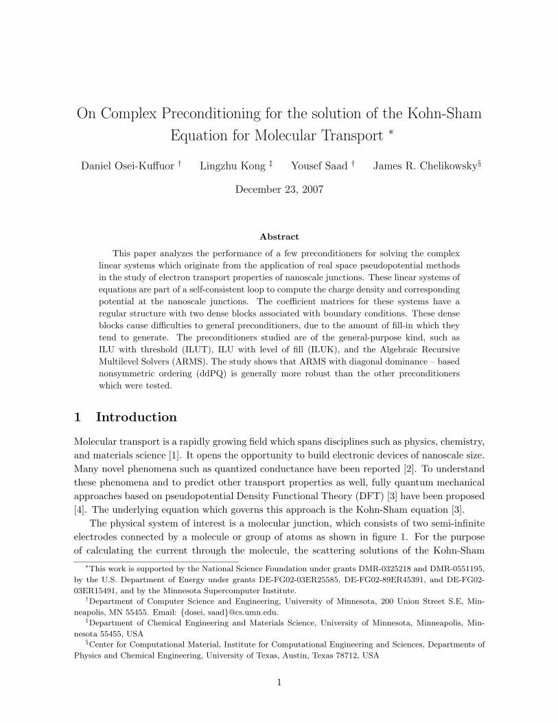
On Complex Preconditioning for the solution of the Kohn-Sham
Equation for Molecular Transport ∗
Daniel Osei-Kuffuor † Lingzhu Kong ‡ Yousef Saad † James R. Chelikowsky§
December 23, 2007
Abstract
This paper analyzes the performance of a few preconditioners for solving the complexlinear systems which originate from the application of real space pseudopotential methodsin the study of electron transport properties of nanoscale junctions. These linear systems ofequations are part of a self-consistent loop to compute the charge density and correspondingpotential at the nanoscale junctions. The coefficient matrices for these systems have aregular structure with two dense blocks associated with boundary conditions. These denseblocks cause difficulties to general preconditioners, due to the amount of fill-in which theytend to generate. The preconditioners studied are of the general-purpose kind, such asILU with threshold (ILUT), ILU with level of fill (ILUK), and the Algebraic RecursiveMultilevel Solvers (ARMS). The study shows that ARMS with diagonal dominance – basednonsymmetric ordering (ddPQ) is generally more robust than the other preconditionerswhich were tested.
1 Introduction
Molecular transport is a rapidly growing field which spans disciplines such as physics, chemistry,and materials science [1]. It opens the opportunity to build electronic devices of nanoscale size.Many novel phenomena such as quantized conductance have been reported [2]. To understandthese phenomena and to predict other transport properties as well, fully quantum mechanicalapproaches based on pseudopotential Density Functional Theory (DFT) [3] have been proposed[4]. The underlying equation which governs this approach is the Kohn-Sham equation [3].
The physical system of interest is a molecular junction, which consists of two semi-infiniteelectrodes connected by a molecule or group of atoms as shown in figure 1. For the purposeof calculating the current through the molecule, the scattering solutions of the Kohn-Sham
∗This work is supported by the National Science Foundation under grants DMR-0325218 and DMR-0551195,
by the U.S. Department of Energy under grants DE-FG02-03ER25585, DE-FG02-89ER45391, and DE-FG02-
03ER15491, and by the Minnesota Supercomputer Institute.†Department of Computer Science and Engineering, University of Minnesota, 200 Union Street S.E, Min-
neapolis, MN 55455. Email: dosei, [email protected].‡Department of Chemical Engineering and Materials Science, University of Minnesota, Minneapolis, Min-
nesota 55455, USA§Center for Computational Material, Institute for Computational Engineering and Sciences, Departments of
Physics and Chemical Engineering, University of Texas, Austin, Texas 78712, USA
1

Figure 1: Diagram depicting the physical system of interest (as in [7]). The incoming wave, ΦinL ,
originating from the left bulk is partially reflected, ΦrefL , back into the left bulk at the boundary of the
transition region, and partially transmitted through the transition region, into the right bulk, ΦtraL .
equation that extend over the entire system are considered. The open boundary conditionsof this system are modeled by the real-space pseudopotential method [7, 4]. The approachinvolves solving complex systems of linear equations, derived from a high order finite differencediscretization of the Kohn-Sham equation, as part of a self-consistent calculation.
This paper presents a comparative study of a number of complex-valued preconditionersto solve these linear systems. The paper is organized as follows: Section 2 describes theformulation of the discretized model and identify interesting numerical properties inherent inthe resulting system. Section 3 introduces the complex-valued preconditioners used in our tests,and Section 4 presents a comparative analysis of their performance on the application problem.A summary of our observations and a conclusion are proposed in section 5.
2 Model Formulation
2.1 Discretization and Linear System Formation
The central equation for the various DFT–based approaches in molecular transport is the Kohn-Sham equation [3]:
−∇2
2ψ(~r) + Veff ψ(~r) = ε ψ(~r), (1)
where ψ(~r) and ε are the Kohn-Sham orbital and eigenvalue respectively. The effective potential,Veff , is defined to be
Veff (~r) = vext(~r) + vH(~r) + vxc(~r) . (2)
Here the vext is the external potential, typically a sum of the ion-core potential centered at theatoms. The next two terms, vH and vxc, are the Hartree potential and exchange-correlationpotential respectively. They have functional dependence on the electron charge density, n,which can be written as the summation of the squares of the occupied Kohn-Sham orbitals
n(~r) =∑
i
|ψi(~r)|2. (3)
2

The Hartee potential is usually evaluated by solving the Poisson’s equation
∇2vH(~r) = −4πn(~r). (4)
The exchange-correlation potential, however, has no known exact form. We used the Wignerapproximation [13]
vxc = −0.985n1/3 − 0.056n2/3 + 0.0059n1/3
(0.079 + n1/3)2. (5)
Using a higher order finite difference approximation for the Laplacian, this equation can bediscretized in real space as [5]
−12
N∑n=−N
[cxnψ(xi + nhx, yj , zk) + cynψ(xi, yj + nhy, zk)
+cznψ(xi, yj , zk + nhz)] + Veff (xi, yj , zk)ψ(xi, yj , zk)
=ε ψ(xi, yj , zk)
(6)
where N is the order of the finite difference expansion. For simplicity, central finite differencesare used in the following derivations. The scalars cµn(µ = x, y, z) represent the expansioncoefficients [6], and hx, hy and hz are the grid spacing in x, y and z directions respectively.
The system is usually assumed to be periodic in the xy-plane, parallel to the nanoscalejunction, so that the wave functions satisfy the Bloch conditions in the x and y directions.Mathematically, one has
ψ(x+ ax, y, z) = eikxaxψ(x, y, z)
ψ(x, y + ay, z) = eikyayψ(x, y, z),(7)
where ax and ay are the periodicities along x and y directions, and kx and ky are the wavevectors.Along the z-direction (perpendicular to the nanoscale junction), the current flows from oneelectrode lead through the molecule, into the other lead. Along this direction the system isaperiodic and Bloch theorem does not hold. The molecular junction, (or transition region),is chosen to be large enough so that the scattering potential is negligible outside it. We thenapply matching conditions to the scattering waves requiring the wave functions to approachasymptotically the eigenfunctions of the bulk electrodes.
As suggested by Fujimoto and Hirose [7], we assign the wave functions on the xy-plane,positioned at zk, in a columnar vector, Ψ(zk) = [ψ(x1, y1, zk), ψ(x2, y1, zk), · · · , ψ(xn, yn, zk)]T .In this notation, Eq. (6), can be rewritten in matrix form as
(E − H)
Ψ(z0)Ψ(z1)
...Ψ(zm+1)
=
B†
zΨ(z−1)0...
BzΨ(zm+2)
(8)
where E, H and Bz are the corresponding eigenvalue, Hamiltonian matrix and coefficient matrixas in [7]. The z coordinates z−1, z0 and zm+1, zm+2 are chosen to be in the left and right bulkregions respectively, while z1, · · · , zm are in the transition region (as shown in figure 1).
3

Now, consider an incoming wave originating from the left bulk electrode. We analyze theboundary conditions along the z-direction as follows: Upon reaching the transition region,this incoming wave is partly reflected back into the left lead and partly transmitted into theright lead by the scattering atom (or molecule). The reflected and transmitted waves willasymptotically take the form of a linear combination of the eigenfunctions of the correspondingelectrode leads. This result may be formally written as:
Ψ(zk) = Φin(zk) +∑
l
rlΦrefl (zk) (9)
for the left bulk region, andΨ(zk) =
∑l
tlΦtral (zk) (10)
for the right bulk region. Here ΦA(A=in (incident), ref (reflected) and tra (transmitted))are the eigenstates of the leads evaluated on the zk plane, and can be obtained by solving ageneralized eigenproblem [7]. The scalars rl and tl are the reflection and transmission coefficientsrespectively.
Note that since z0 and z−1 are both in the left region, the wave functions on these two planessatisfy the same Eq. (9). In order to avoid numerical instability (see [7]), we reformulate Eq. (9)by eliminating the reflection coefficients rl, to obtain Ψ(z−1) expressed in terms of Ψ(z0) asfollows:
Ψ(z−1) = Φin(z−1) +Q(z−1)Q−1(z0)(Ψ(z0)− Φin(z0)) (11)
with Q(zk) = [Φ1(zk),Φ2(zk), · · · ,Φn×n(zk)]. Similarly, for the right region, one has:
Ψ(zm+2) = Q(zm+2)Q−1(zm+1)Ψ(zm+1) (12)
Substituting Eq. (11) and (12) into Eq. (8), one obtains for left incoming waves (i.e. originatingfrom the left bulk electrode) Φin
L :
(E − H − H)
Ψ(z0)Ψ(z1)
...Ψ(zm+1)
=
Ω0...0
(13)
where H represents the matrix of boundary conditions in the z direction. It is essentially azero matrix, except that it contains two dense blocks in the upper left and lower right regionsof the matrix, corresponding to B†
zQ(z−1)Q−1(z0) and BzQ(zm+2)Q−1(zm+1), for the left andright bulk regions respectively. The size of these dense blocks is typically αznxy by nxy, whereαz is the order of the finite difference expansion in the z direction, and nxy is the number ofgrid points in one z slice plane. Here, Ω = B†
z[ΦinL (z−1) − Q(z−1)Q−1(z0)Φin
L (z0)]. A similarequation can be obtained for the right incoming waves (i.e. originating from the right bulkelectrode).
See [4] for more details on the formulation of the linear system.
4

2.2 Numerical Properties
Equation (13) defines the final form of the linear system we wish to solve. The operator,A = (E − H − H), is a relatively sparse complex matrix except for the two dense blockscontributed by H. The matrix A is also not diagonally dominant and the contribution from H
makes it neither symmetric nor hermitian. Moreover, the properties of A are highly dependenton the value of the incoming wave vector k. The solution of these types of linear systemsfor high values of k has been recognized as one of the most challenging problems for modernnumerical techniques [14].
Figure 2 shows the structure of the matrix A, for the above linear system in Eq. (13). Here,the number of grid points in the x, y and z directions are 12, 12, and 28 respectively, and afourth-order finite difference expansion was used for all three directions, resulting in a matrixof size 4032.
In the structure, we observe the dense blocks in the upper-left, and lower-right corners,corresponding to H. The main diagonal contains the Kohn-Sham energy E and the local partof the potential. The fourth-order finite difference expansion of the hamiltonian along the xand y directions contribute to the block structure along the main diagonal. The block regionat the center of the diagonal (and the matrix) represents contributions from the non-local partof the potential. The non-zero regions above and below the main diagonal blocks represent thefourth-order finite difference expansion of the hamiltonian, in the z direction.
As mentioned earlier, the choice of the wave vector k, for the incoming wave, dictates thelevel of difficulty for the numerical solution of the system in Eq. (13). High values of k tendto shift the spectrum of the matrix to the right and generate more complex eigenvalues, thusmaking the resulting system very indefinite. The typical range of values for the components ofthe wave vector is (0.0, 1.0).
Figure 3 shows the eigenvalue spectrum of the matrix in Eq. (13). Figure (3a) shows the
Figure 2: Structure of the matrix in Eq. (13). (nx, ny, nz) = (12, 12, 28), and (αx, αy, αz) = (4, 4, 4)respectively.
5

(a) (b)
Figure 3: Eigenvalue spectrum of the matrix in Eq. (13). (a) - With wave vector k = (0.1, 0.1, 0.1); (b)- With wave vector k = (0.9, 0.9, 0.9).
spectrum of the matrix with wave vector k = (0.1, 0.1, 0.1), and figure (3b) shows the spectrumof the matrix with wave vector k = (0.9, 0.9, 0.9). From the figures, we observe the shift in thespectrum from left to right, resulting in a greater degree of clustering of the eigenvalues aroundzero, for the case with the higher wave vector. Furthermore, we observe a greater number ofcomplex eigenvalues in (b), compared to (a). Thus we can clearly see that solving the systemwith the matrix corresponding to (b) will be more numerically challenging, compared withsolving the system with the matrix corresponding to (a).
2.3 Related Formulations
The open boundary conditions of this system are often treated by two approaches. One approachmakes use of the “nonequilibrium Green function method” [8] combined with DFT. The otherapproach solves the “Lippmann-Schwinger” [9] equation to obtain the scattering states. Inboth approaches, the open boundary conditions are incorporated into the Green’s function ofthe bare electrodes, and used to calculate the electronic structure and transport properties ofthe system. A number of techniques have been applied to obtain the Green’s function and thescattering states by exploiting different bases [10, 11, 12].
An alternate approach, the one considered in the preceding sections, is to solve the Kohn-Sham equation directly in real space, without any explicit basis. One advantage of this approachis that the open boundary conditions can be easily treated in real space. Moreover, the resultingHamiltonian is sparse, and efficient sparse solvers can be used. Fujimoto and Hirose recentlyproposed a real space formalism that models the system [7]. The approach implements a finitedifference discretization of the Kohn-Sham equation to obtain the global states and conductance.Furthermore, the approach requires that a large Hamiltonian matrix be inverted in solving forthe wave functions. This can be very computationally expensive.
The formulation presented in this paper follows the approach in [7] but avoids direct in-versions of the Hamiltonian matrix, by transforming the equations into a set of simultaneous
6

linear equations.
3 Solution Methods
We can rewrite the system (13) using standard notation of linear algebra as
Ax = b. (14)
Since the original linear system is intrinsically 3-dimensional in nature, it is advisable to avoidthe use of direct methods as they tend to be quite expensive both in terms of memory andcomputations. Preconditioned Krylov subspace methods [16] are considered as the most general-purpose iterative techniques available and offer a good compromise between the robustnessof direct solvers and the effectiveness of special purpose procedures such as multigrid. Forcompleteness we begin with a brief background on these methods.
A preconditioned Krylov subspace method for solving the linear system (14) consists of anaccelerator and a preconditioner [16]. In what follows we call M the preconditioning matrix,so that, for example, the right-preconditioned system
AM−1y = b where x = M−1y (15)
is solved instead of the original system (14). The above preconditioned system is solved viaan “accelerator”, a term used to include a number of methods of the Krylov subspace class.Thus, given an inital guess x0 to the solution, and r0 = b − Ax0 its initial residual, a right-preconditioned Krylov subspace method computes an approximate solution from the affinespace
x0 + Spanr0, AM−1r0, · · · ,(AM−1
)m−1r0, , (16)
which verifies certain conditions. For example, the GMRES algorithm [16] requires that theresidual rm = b − Axm has a minimal 2-norm among all possible approximate solutions fromthe affine Krylov subspace shown above.
3.1 Incomplete LU factorizations
The most common way to define the preconditioning matrix M is through Incomplete LUfactorizations. An ILU factorization is obtained from an approximate Gaussian eliminationprocess. When Gaussian elimination is applied to a sparse matrix A, a large number of nonzeroelements may appear in locations originally occupied by zero elements. These fill-ins are oftensmall elements and may be dropped to obtain Incomplete LU factorizations.
The simplest of these procedures, ILU(0) is obtained by performing the standard LU factor-ization of A and dropping all fill-in elements that are generated during the process. Thus, theL and U factors have the same pattern as the lower and upper triangular parts of A (respec-tively). More accurate factorizations denoted by ILU(k) have been defined which drop fill-insaccording to their ‘levels’ in the elimination process, where the levels attempt to reflect sizeand are defined recursively [16]. It is most common to use these techniques with levels of fillnot exceeding 2 in practice, as higher levels of fill lead to more expensive factorizations, bothin terms of storage and computations.
7

Another class of preconditioners is based on dropping fill-ins according to their numericalvalues. One of these methods is ILUT (ILU with Threshold). This procedure uses basically aform of Gaussian elimination which generates the rows of L and U one by one. Small valuesare dropped during the elimination, using a parameter τ . A second parameter, p, is then usedto keep the largest p entries in each of the rows of L and U . This procedure is denoted byILUT (τ, lfil) of A.
3.2 Multilevel ILUs and ARMS
A related class of preconditioners developed in [18, 24] exploit the idea of multi-level or multi-stage factorization. The original coefficient matrix is symmetrically permuted to the form
A = P
(B F
E C
)P T (17)
in which the B block is block diagonal. Such a structure is obtained by using independent set- or group-independent set orderings. The Algebraic Recursive Multilevel Solver (ARMS, [18])exploits such orderings to define multilevel techniques. Thus, at the l-th level, the coefficientmatrix is reordered as in (17) where B is block-diagonal and then the following block factoriza-tion is computed ‘approximately’ (subscripts corresponding to level numbers are introduced):(
Bl Fl
El Cl
)≈
(Ll 0
ElU−1l I
)×
(Ul L−1
l Fl
0 Al+1
), (18)
whereBl ≈ LlUl Al+1 ≈ Cl − (ElU
−1l )(L−1
l Fl) (19)
There are essentially two main steps to the procedure. First, obtain a group-independentset and reorder the matrix in the form (17); second, obtain an ILU factorization Bl ≈ LlUl
for Bl and approximations to the matrices L−1l Fl, ElU
−1l , and Al+1. The process is repeated
recursively on the matrix Al+1 until a selected number of levels is reached. At the last level,a simple ILUT factorization, possibly with pivoting, or an approximate inverse method can beapplied.
The Ai’s remain sparse but become denser as the number of levels increases, so smallelements are dropped in the block factorization to maintain sparsity. Note that the matricesElU
−1l , L−1
l Fl or their approximations Gl ≈ ElU−1l and Wl ≈ L−1
l Fl which are used to obtainthe Schur complement Al+1 via (19) need not be saved. They are computed only for the purposeof obtaining an approximation to Al+1 and are discarded thereafter to save storage. Subsequentoperations with L−1
l Fl and ElU−1l are performed using Ul, Ll and the blocks El and Fl.
3.3 Use of nonsymmetric permutations
Instead of insisting that the matrix B in (17) be block diagonal, we can try to reorder it insuch a way that the B block has some “good” numerical properties, specifically of diagonaldominance. The rationale is that a poor B block will have a negative impact on the rest of the
8

factorization. ARMS-ddPQ uses nonsymmetric factorizations with this goal in mind. Insteadof (17), we now use two permutations, one for the rows and the other for columms:
A = P
(B F
E C
)QT . (20)
No particular structure is required of B, but the permutations are selected so that the B blockis as diagonally dominant as possible. The name of the procedure for obtaining the permutationis diagonal-dominance PQ (ddPQ) ordering. The rest of the multi-level procedure is identicalwith that of ARMS. In other words, the only difference between ARMS-ddPQ and ARMS liesin the permutations used to put the matrix at the l-th level in 2× 2 block form.
It is also possible to use nonsymmetric permutations in the context of ILUT. The methodknown as ILUT with pivoting, see [16], implements a column pivoting ILU, so in effect, we haveAQ ≈ LU . In this case, only the columns are permuted. ILUTP is known to be somewhatmore robust than ILUT at the condition to allow substantially more fill-in.
4 Numerical Results
We apply the above preconditioning techniques to solve a test system consisting of a single Featom between the two electrodes. A fourth-order finite difference scheme is used for all thedirections. The number of grid points in the x, y, and z planes are 24, 24, and 54 respectively.The resulting system has size 31,104 with 3,577,008 nonzero elements. We allow a maximum of1500 iterations, with a convergence tolerance of 1.0 x 10⁻⁶. To measure memory cost, we usethe fill-factor which is defined as the ratio of the number of nonzero entries for the LU factorsto the number of nonzero entries in A. In all cases, the maximum fill factor allowed is 4.0. Theaccelerator used for all tests is the restarted GMRES, with a restart dimension of m = 120,which is the maximum dimension of the subspace (16) before restarting the process.
We present results for the system with different values for the wave vector. For each testcase, we solve two systems, each corresponding to an orientiation of the electron spin - (“spin-up” and “spin-down”). However, we construct the preconditioner only once, and use it to solveboth systems each time. The number of iterations and the iteration time is then averaged overthese two solves. For the ILUK approach, we chose the level of fill parameter to be = 1, as thiswas the largest level of fill for which the fill-factor does not exceed 4.
Table 1 shows results of tests involving the ILUK, ILUT, and ARMS-ddPQ preconditioners.The results show a limitation in the performance of the ILUK preconditioner for higher-valuedwave vectors. Increasing the level of fill parameter may result in better convergence at the costof severely compromising memory efficiency. For example, in the above tests, allowing a levelof fill parameter = 2 (instead of 1) resulted in a fill factor (memory cost) of ≈ 8.0. The ILUTpreconditioner, on the other hand, performed quite well for all three test cases, converging withina reasonable number of iterations and within the required limits of memory cost. However,clearly ARMS-ddPQ outperforms the rest when taking into account both convergence andmemory efficiency.
To better understand the performance of the ARMS-ddPQ technique and how it compareswith ILUT, we construct a small test problem and show the effect of the two approaches on the
9

Preconditioner k = (kx, ky, kz) No. iters Setup Time (s) Iter. Time (s) Fill Factor
ILU(1)
(0.11, 0.11, 0.12) 120 101 11.32 3.18
(0.55, 0.55, 0.65) 1500 94.50 257.50 3.18
(0.91, 0.91, 1.00) 1500 96.00 273.50 3.18
ILUT
(0.11, 0.11, 0.12) 14 23.30 2.34 1.71
(0.55, 0.55, 0.65) 103 69.40 27.10 3.52
(0.91, 0.91, 1.00) 67 51.30 16.25 3.07
ARMS-ddPQ
(0.11, 0.11, 0.12) 13 30.80 2.41 1.49
(0.55, 0.55, 0.65) 21 39.80 4.76 2.13
(0.91, 0.91, 1.00) 12 51.80 2.91 2.69
Table 1: Comparison of preconditioners on application problem with different wave numbers. Thenumber of iterations and the iteration time is averaged over the two realizations of electron spin.
preconditioned matrices. The test problem is of size 3,456, with 244,928 nonzero entries, andthe number of grid points in the x, y and z planes are 12, 12, and 24 respectively. We chose thewave vector to be k = (0.55, 0.55, 0.95), and we set the fill factor to be fixed at ≈ 2.0. Table2 shows a summary of the results. As before, we observe a better convergence performancein terms of iteration count for ARMS-ddPQ. To show the effect of the preconditioners thatproduced these results, we analyze the spectrum of the preconditioned matrices obtained byapplying each of these preconditioners to the above test problem. Our iterative solver approachimplements right preconditioning:
Ax = b ≡ AM−1y = b, (21)
where y = Mx and M is the preconditioner. It is known that eigenvalues of preconditionedmatrices do not fully explain the convergence behavior of iterative methods, due in part to theeffects of high departures from normality [16]. However, in practical situations involving PDEs,a clustering of eigenvalues around one is generally highly desirable.
Figure 4 shows the eigenvalue spectrum of the original matrix (a), the ILUT preconditionedmatrix (b), and the ARMS-ddPQ preconditioned matrix (c) respectively. Figure 5 shows thedetails of the dense cluster regions of the spectrum of the preconditioned matrices.
From figure 4 we observe that both preconditioning techniques do a decent job of clusteringthe eigenvalues around the point (1, 0). Blowing up these cluster regions (figure 5), we observea marked difference between the two spectra. For the ILUT preconditioned matrix, we observethat the majority of the eigenvalues in the dense cluster region are complex - (figure 5a). Forthe ARMS-ddPQ preconditioned matrix, a significant proportion of the eigenvalues in the densecluster region lie closer to the real line - (figure 5b). In fact, the clustering appears to be betterthan that achieved by ILUT, with the additional characteristic that it is along the real line,leading to fewer complex eigenvalues.
Preconditioner No. iters Setup Time (s) Iter. Time (s) Fill Factor
ILUT 75 0.979 0.819 2.0
ARMS-ddPQ 17 2.49 0.169 2.0
Table 2: Comparison of the ILUT and ARMS-ddPQ preconditioners on a small test problem. Wavenumber k = (0.55, 0.55, 0.95).
10

−10 −8 −6 −4 −2 0 2 4 6 8 10 12 14 15−0.02
0
0.02
0.04
0.06
0.08
0.1
0.12
real
imag
inar
y
eigenvalue spectrum of the original matrix
(a)
(b) (c)
Figure 4: Spectra of the preconditioned matrices for the small test problem. (a) Original matrixk = (0.55, 0.55, 0.95); (b) ILUT preconditioned matrix; (c) ARMS-ddPQ preconditioned matrix.
4.1 Column Pivoting
In order to alleviate some of the shortcomings of the standard ILUT technique [16], the ILUTPapproach implements some form of one-sided nonsymmetric pivoting (usually column partialpivoting) in the construction of the preconditioner. The resulting preconditioner is generallymore robust than ILUT, but is less memory efficient since ILUTP tends to generate more fill-in
11

(a) (b)
Figure 5: Enlarged dense regions of eigenvalue spectra (magnification = 5x). (a) ILUT preconditionedmatrix; (b) ARMS-ddPQ preconditioned matrix.
[16, 20]. We analyze the effect of column pivoting on this application problem by comparingthe performance of ILUT with that of ILUTP on a number of test cases.
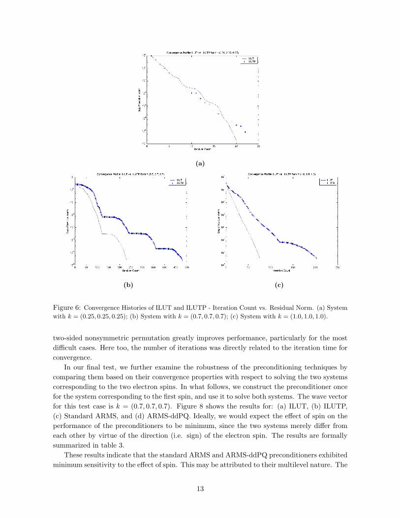
In figure 6, we show the convergence profiles when solving three different systems using theILUT and ILUTP preconditioning techniques. Each system is of size 31,104 with 3,577,008nonzero elements as before. To allow for a good comparison with difficult cases too, we fixedthe fill factor at 4.0 for both preconditioners for all test cases. The profile depicts convergencefor solving each system corresponding to the first spin direction only (“spin-up”). Figure 6(a) shows results for a system with k = (0.25, 0.25, 0.25), (b) shows results for a system withk = (0.7, 0.7, 0.7), and (c) shows the results for a system with k = (1.0, 1.0, 1.0).
Interestingly, the results show that the ILUT approach performs better than ILUTP for allthree cases. This may be attributed to the fact that performing column partial pivoting candestroy some good structural properties of the matrix that benefit the ILUT technique. Anotherexplanation is that ILUTP requires more memory to work well and limiting the fill-factor to4, puts it at a big disadvantage. The more indefinite the system is, the greater the effect ofpivoting, and we observe convergence for ILUT in less than half the number of iterations forthe ILUTP approach. Also, note that the number of iterations for each of these test cases wasdirectly proportional to the iteration time for convergence.
4.2 Symmetric and Nonsymmetric Permutation
To examine the effect of symmetric and nonsymmetric permutations on our system, we comparethe performance of standard (symmetric) ARMS and ARMS-ddPQ on the same three test casesas in the preceding example.
Figure 7 shows the convergence profiles of solving the three systems using the standardARMS and ARMS-ddPQ preconditioning techniques. Note that the results for the last case,7(c), has been truncated to show only up to 100 iterations, since standard ARMS failed toconverge after the 1500 maximum allowed iterations. The results indicate that implementing a
12
(a)
(b) (c)
Figure 6: Convergence Histories of ILUT and ILUTP - Iteration Count vs. Residual Norm. (a) Systemwith k = (0.25, 0.25, 0.25); (b) System with k = (0.7, 0.7, 0.7); (c) System with k = (1.0, 1.0, 1.0).
two-sided nonsymmetric permutation greatly improves performance, particularly for the mostdifficult cases. Here too, the number of iterations was directly related to the iteration time forconvergence.
In our final test, we further examine the robustness of the preconditioning techniques bycomparing them based on their convergence properties with respect to solving the two systemscorresponding to the two electron spins. In what follows, we construct the preconditioner oncefor the system corresponding to the first spin, and use it to solve both systems. The wave vectorfor this test case is k = (0.7, 0.7, 0.7). Figure 8 shows the results for: (a) ILUT, (b) ILUTP,(c) Standard ARMS, and (d) ARMS-ddPQ. Ideally, we would expect the effect of spin on theperformance of the preconditioners to be minimum, since the two systems merely differ fromeach other by virtue of the direction (i.e. sign) of the electron spin. The results are formallysummarized in table 3.
These results indicate that the standard ARMS and ARMS-ddPQ preconditioners exhibitedminimum sensitivity to the effect of spin. This may be attributed to their multilevel nature. The
13

(a)
(b) (c)
Figure 7: Convergence Histories of standard ARMS and ARMS-ddPQ - Iteration Count vs. ResidualNorm. (a) System with k = (0.25, 0.25, 0.25); (b) System with k = (0.7, 0.7, 0.7); (c) System withk = (1.0, 1.0, 1.0).
difficulty for standard numerical solvers to solve a particular problem depends largely on theproperties of the model. By their nature, multilevel methods automatically build smaller scalemodels, that exploit the “nice” properties of the linear system, and that could be aggregatedto solve the original problem. This key feature of multilevel methods allows the performanceof the standard ARMS and ARMS-ddPQ preconditioning techniques to be much less sensitive
Preconditioner Spin 1 (“spin-up”) Spin 2 (“spin-down”)
ILUT 228 284
ILUTP 476 583
Standard ARMS 57 59
ARMS-ddPQ 11 13
Table 3: Table of results for the number of iterations required to solve the two systems correspondingto each electron spin direction.
14

(a) (b)
(c) (d)
Figure 8: Convergence Histories for solving two systems corresponding to each electron spin direction,with each preconditioner constructed only once - k = (0.7, 0.7, 0.7). Iteration Count vs. Residual Norm.(a) ILUT; (b) ILUTP; (c) Standard ARMS; (d) ARMS-ddPQ
to small changes due to spin, than the other techniques.The results seem also to indicate that multilevel-type methods are less sensitive to small
changes in the system. From figures 6, 7, and 8 we see a marked difference in the shape ofthe profiles for the ILUT and ILUTP methods, compared with multilevel methods. The ILUTand ILUTP techniques exhibit a stepped profile with a frequency of 120 which is the restartdimension for GMRES. The multilevel methods converge before reaching the restart dimensionof 120, and so this phenomenon is not observed in the corresponding convergence curves.
5 Conclusion
In this paper, we have analyzed the performance of some ILU-based preconditioners to solvehighly indefinite systems that result from an application in molecular transport. Among thepreconditioners tested, we have shown that the ARMS-ddPQ technique performs best, in terms
15

of storage and computational cost. The method builds the preconditioning matrix from amultilevel ILU approach, combined with a diagonal-dominance criterion for permuting thematrix in a nonsymmetric way. ARMS-ddPQ implements dropping techniques to reduce fill-inand preserve sparsity. It also includes a number of parameters that can be adjusted to obtaina robust preconditioner for the particular problem at hand.
For most indefinite problems, performing some form of nonsymmetric permutation [21, 23,22] during the incomplete factorization tends to improve the performance of the numericalsolver. Two such approaches are the ILUT factorization with partial pivoting, and ARMS withnonsymmetric permutations (i.e. ddPQ ordering). For the problems in the application studiedin this paper, one-sided column partial pivoting techniques such as ILUTP resulted in a worseperformance compared with standard ILUT. However, within a multilevel approach, such asARMS, nonsymmetric permutations can be very beneficial. Thus, a two-sided nonsymmetricpermutation approach, such as ARMS with ddPQ ordering, showed significant improvement inperformance over standard ILU methods and standard ARMS (with symmetric permutations).
The standard version of ARMS (symmetric permutations) performed better than ILUTand ILUTP for the cases with low and average difficulty, but failed to converge for the mostdifficult problems. This may be attributed to the implementation of symmetric permutationsto reorder the matrix. For highly indefinite systems, this symmetric reordering can result in apreconditioned matrix with poor properties.
References
[1] M.C. Petty, M.R. Bryce and D. Bloor(Eds.), Introduction to molecular Electronics, OxfordUniversity Press , New York, 1995.
[2] H. Ohnishi, Y. Kondon and K. Takayanagi, Nature, 398, 780 (1998).
[3] P. Hohenberg and W. Kohn, Phys. Rev. 136, B864 (1964); W. Kohn and L.J. Sham, Phys.Rev. 140, A1133 (1965).
[4] L. Kong, M.L. Tiago and J.R. Chelikowsky, Phys. Rev. B, 73, 195118 (2006).
[5] J.R. Chelikowsky, N. Troullier, and Y. Saad, Phys. Rev. Lett. 72, 1240 (1994).
[6] B. Fornberg and D.M. Sloan, in Acta numerica 94 , edited by A. Iserles, CambridgeUniversity Press, Cambridge, UK, 1994.
[7] Y. Fujimoto and K. Hirose, Phys. Rev. B, 67, 195315 (2003).
[8] S. Datta, Electronic Transport in Mesoscopic Systems (Cambridge University Press, Cam-bridge, UK, 1997).
[9] N. D. Lang, Phys. Rev. B, 52, 5335 (1995).
[10] H. Ness and A. J. Fisher, Phys. Rev. B, 56, 12469 (1997).
[11] P. S. Damle, A. W. Ghosh, and S. Datta, ibid, 64, 201403(R) (2001).
16

[12] J. J. Palacios, A. J. Perez-Jimenez, E. Louis, and J.A. Verges, ibid, 64, 115411 (2001).
[13] E. P. Wigner, Phys. Rev. 46, 1002 (1934).
[14] O. Zienkiewicz, Achievements and some Unsolved Problems of the Finite Element Method.Int. J. Numer. Mthds. Eng. 47, 9-28 (2000).
[15] R. Kechroud, A. Soulaimani, Y. Saad and S. Gowda, Preconditioning techniques for thesolution of the Helmholtz equation by the finite element method. Math. Comput. Simul.65, 4-5 (2004), 303-321.
[16] Y. Saad, Iterative Methods for Sparse Linear Systems, 2nd edition. SIAM, Philadelphia,PA, (2003)
[17] Z. Li, Y. Saad and M. Sosonkina, pARMS: A parallel version of the Algebraic RecursiveMultilevel Solver. nlaa, 10, (2003) 485-509
[18] Y. Saad, B. Suchomel, ARMS: An Algebraic Recursive Multilevel Solver for general SparseLinear Systems. nlaa, 9, (2002)
[19] M. Sosonkina, Y. Saad and X. Cai, Using the parallel Algebraic Recursive Multilevel Solverin modern physical applications. Future generation Comoptur Systems, 20, (2004), 489-500
[20] D. Osei-Kuffuor and Y. Saad, A Comparison of Preconditioners for Complex Valued Ma-trices, submitted to nlaa: NLA-07-0029.
[21] M. Benzi, J. C. Haws, and M. Tuma, Preconditioning Highly Indefinite and NonsymmetricMatrices. Siam Journal on Scientific Computing, 22, 4(2001), 1333-1353
[22] I.S. Duff, and J. Koster, On algorithms for permuting large entries to the diagonal of asparse matrix. SIAM Journal on Matrix Analysis and Applications, 22, 4(2001), 973-996
[23] M. Olschowka, and A. Neumaier, A new pivoting strategy for Gaussian elimination. LinearAlgebra and its Applications, 240, 1-3(1996), 131-151
[24] Y. Saad, Multilevel ilu with reorderings for diagonal dominance. SIAM J. Sci. Comput.,27, 3(2005), 1032-1057
17