on coherent structures in a separated/reattached flo · on coherent structures in a...

On coherent structures in a separated/reattached flow

ZHIYIN YANG1 and IBRAHIM E ABDALLA2

1Department of Aeronautical and Automotive Engineering Loughborough University Loughborough LE11 3TU

UNITED KINGDOM [email protected] http://www.lboro.ac.uk/departments/tt/staff/yang.html

2School of Engineering and Technology De Montford University

Leicester LE1 9BH UNITED KINGDOM [email protected]

http://www.dmu.ac.uk/faculties/cse/about_cse/contact/staff/staff_ibrahim_abdalla.jsp

Abstract: It is well known that large-scale organised motions, usually called coherent structures, exist in many transitional and turbulent flows. The topology and range of scales of coherent structures change widely in different flows. However, it is not well established what kind of large-scale coherent structures exists in separated/reattached transitional flows. Large Eddy Simulation (LES) with a dynamic subgrid-scale model is employed to investigate a separated boundary layer transition under 2% free stream turbulence level and without free stream turbulence on a flat plate with a blunt leading edge. Flow visualization is employed to show the entire transition process leading to breakdown to turbulence and large-scale coherent structures have been identified at various stages of the transition process. However, there are some noticeable difference between the flow case with and without free stream turbulence. The Kelvin-Helmholtz rolls, which are clearly visible under no free stream turbulence (NFST), are not so clearly visible under 2% free steam turbulence (FST) case. The Lambda-shaped vortical structures which can be clearly seen in the NFST case can hardly be identified in the FST case. Generally speaking, the effects of free-stream turbulence have led to an early breakdown of the separated boundary layer and hence increased the randomisation in the vortical structures, degraded the spanwise coherence of those large-scale structures. Key-Words: Large-eddy simulation; large-scale coherent structures; free stream turbulence; transition 1 Introduction It has been established that spatially coherent and temporally evolving vortical structures, popularly called coherent structures (CS) [1], exist in turbulent shear flows. The presence of CS in turbulent shear flows was first suggested by Townsend [2] but they were also noticed in the early experiments of Corrsin [3]. Those structures are usually different from flow to flow and seem to be strongly dependent on the flow geometry, the flow condition and the location with respect to solid-surfaces. For example, large-scale spanwise vortices appear to dominate the dynamics in plane mixing layer [4] while dominant structures of the transitional plane boundary layer may be a Lambda-shaped vortex and low-speed streaks [5]. In wakes, counter-rotating vortices are known to dominate the flow dynamics [6].

The discovery of coherent structures has changed the classical view that turbulent flows are random fluid motions in a state of total chaos. It is also quite exciting because the time evolution of a deterministic structure might be mathematical tractable. Therefore, understanding the evolution and interaction of CS and coupling of CS with background turbulence is very important not only for having a better insight into turbulence phenomena such as entrainment and mixing, heat and mass transfer, chemical reaction and combustion, drag and aerodynamic noise generation, but also for viable modelling of turbulence [7]. Considerable efforts have been devoted to the subject of coherent structures in turbulent flows and a wide range of investigations have been carried out to try to have a better understanding of CS and their dynamical roles in turbulence. The starting point is, of course, to identify CS in different flow situations.

WSEAS TRANSACTIONS on FLUID MECHANICS Zhiyin Yang and Ibrahim E. Abdalla

ISSN: 1790-5087 143 Issue 2, Volume 3, April 2008

mailto:[email protected]

http://www.lboro.ac.uk/departments/tt/staff/yang.html

mailto:[email protected]

http://www.dmu.ac.uk/faculties/cse/about_cse/contact/staff/staff_ibrahim_abdalla.jsp

Generally speaking, the following five methods can be used to identify CS. 1. Wavelets. 2. Conditional sampling (VITA, LSE). 3. Pattern recognition. 4. Proper orthogonal decomposition POD. 5. Flow Visualisation. Since flow visualisation with recourse to LES has been used in the present study and hence the other four methods will not be discussed here and can be found elsewhere [5,6, 8-10]. Traditionally, flow visualization has been used to reveal flow structures. However, one has to bear in mind that how well and how clearly the flow structures can be shown depends on the visualization schemes used. A high vorticity modulus, Ω, is a possible candidate, especially in free shear flows. For instance, Comte et al. [11] extensively discussed the dynamics of streamwise vortices in mixing layer on the bases of Ω-isosurfaces. In the wall bounded flows, however, the shear created by the no-slip condition on the solid wall is usually significantly higher than the typical intensity of the near-wall vortices. Iso-surfaces of low-pressure have been used by Comte et al. [11] in their investigation of CS in a turbulent boundary layer, indicating the superiority of pressure as a vortex visualization criterion rather than the vorticity modulus. This is also confirmed by Yang [12] using iso-surfaces of low-pressure to visualize large-scale 3D vortical structures in a separated boundary layer transition on a flat plate with a semi-circular leading edge. However, in regions of high concentration of vortices, this criterion may fail to capture the details of the vortical structures. A criterion which shares some properties with both the vorticity and the low-pressure iso-surface is the Q-criterion named after the second invariant of velocity gradient tensor by Hunt et al. [13]. Q is defined as:

)(21

ijijijij SSQ −ΩΩ=

Where

)(21

i

j

j

iij x

uxu

∂

∂−

∂∂

=Ω , )(21

i

j

j

iij x

uxu

S∂

∂+

∂∂

=

Q represents the balance between the rotation rate and the strain rate and positive Q iso-surfaces isolate areas where the strength of rotation

overcomes the strain, thus making those iso-surfaces eligible as vortex envelops. Flow separation and transition plays a very important role engineering flows and hence numerous experimental and numerical studies have been carried out in this area [14-25]. However, there are not many studies focus specifically on the coherent structures. In the present study, a blunt plate is kept parallel to an oncoming stream so that flow separates at the leading edge and reattaches on the surface of the plate at a downstream location. The reattachment process of a separated shear layer is known to be strongly influenced by rolling-up and growth of large-scale vortices, which shed from the separation bubble. Visualizations of the large-scale vortices over a blunt plate without free stream turbulence are few and mainly coming from experimental work. Limited instantaneous 2D snap shots were taken by Cherry et al. [14] and Sasaki & Kiya [15]. Hwang et al. [16] used a smoke wire and a high speed camera to delineate the unsteady process of large-scale vortices in the separated shear layer over a blunt plate geometry. However, their data were also limited to 2D and at very low Reynolds number (Re = 560 based on the plate thickness). The free stream turbulence has a great impact on the transition process and the large-scale vortices. Hillier & Cherry [17] showed that increasing free-stream turbulence level would produce considerable contraction of the bubble length. Kalter & Fernholz [18] studied the effect of free-stream turbulence on a boundary layer with an adverse pressure gradient and a closed reverse-flow region. They found that by adding free-stream turbulence the mean reverse-flow region was shorten or completely eliminated. However, visualizations of the behaviour of large-scale structures from those experimental studies under free stream turbulence are very limited. In addition, very few LES and DNS studies of coherent structures in a separated boundary layer transition have been carried out, especially regarding the effect of free-stream turbulence on the large-scale structures. In this paper, extensive visualization of 3D data resulting from LES studies of a separated boundary layer transition will be presented. Focus will be on the identification of large-scale coherent structures at various stages of transition process and their 3D behaviours, and also trying identify if there are similar large-scale structures in the FST case as in the NFST case, investigating the effects of FST on the structures and on the transition process.



2 Mathematical Formulation The implicitly filtered governing equation expressing conservation of mass and momentum in a Newtonian incompressible flow can be written as

0=∂ ii u (1)

)(2)()( ijeffjijijit spuuu ν∂+−∂=∂+∂ (2)

Where p is the filtered pressure divided by density and νeff is the sol called effective viscosity (molecular viscosity + subgrid scale viscosity) and

ijs is

)(21

ijjiij uus ∂+∂= (3)

The Poisson equation for pressure can be derived by taking the divergence of (2)

)(2)()( ijeffjiiijijiiti Spuuu ν∂∂+∂−∂=∂∂+∂∂ (4)

By using equation (1) one finally obtains

iiji Hpp ∂=Δ=∂∂ 2 (5) Where

)2( ijeffjiji SuuH ν+−∂= (6) It is computationally very expensive to solve equation (5) for 3D high Reynolds flows and one way to speed up the solution is to Fourier transform the equation in z direction to obtain a set of decoupled 2D equations, which in Cartesian form are given by

Rpkyp

xp

z~~~~

22

2

2

2

=−∂∂

+∂∂

(7)

Provided flow is homogeneous in z direction so that a periodic boundary condition can be applied. is the discrete Fourier wave number given as

zk

zkk z

z Δ=

)2/sin(2 (8)

The two-dimensional equation (7), one for each value of can be solved very quickly even when the geometry is complex as long as flow is homogeneous in z direction.

zk

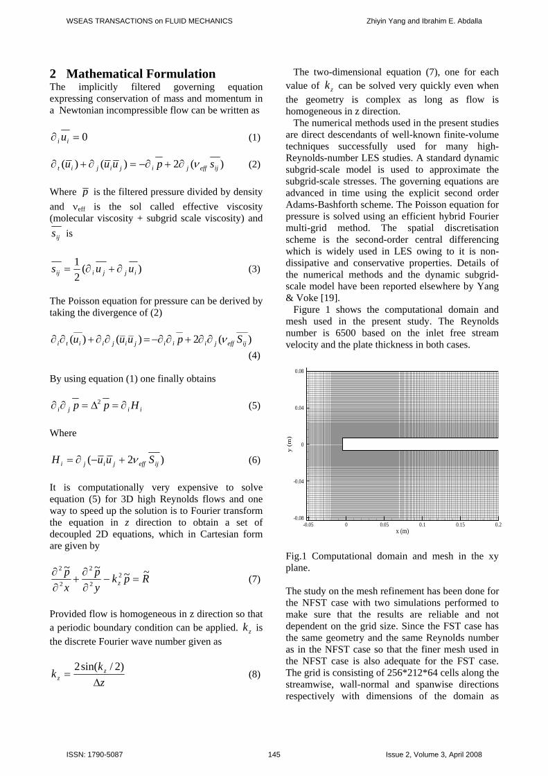
The numerical methods used in the present studies are direct descendants of well-known finite-volume techniques successfully used for many high-Reynolds-number LES studies. A standard dynamic subgrid-scale model is used to approximate the subgrid-scale stresses. The governing equations are advanced in time using the explicit second order Adams-Bashforth scheme. The Poisson equation for pressure is solved using an efficient hybrid Fourier multi-grid method. The spatial discretisation scheme is the second-order central differencing which is widely used in LES owing to it is non-dissipative and conservative properties. Details of the numerical methods and the dynamic subgrid-scale model have been reported elsewhere by Yang & Voke [19]. Figure 1 shows the computational domain and mesh used in the present study. The Reynolds number is 6500 based on the inlet free stream velocity and the plate thickness in both cases.

x (m)

y(m

)

-0.05 0 0.05 0.1 0.15 0.2-0.08

-0.04

0

0.04

0.08

Fig.1 Computational domain and mesh in the xy plane. The study on the mesh refinement has been done for the NFST case with two simulations performed to make sure that the results are reliable and not dependent on the grid size. Since the FST case has the same geometry and the same Reynolds number as in the NFST case so that the finer mesh used in the NFST case is also adequate for the FST case. The grid is consisting of 256*212*64 cells along the streamwise, wall-normal and spanwise directions respectively with dimensions of the domain as



25D*16D*4D. The lateral boundaries are at 8D away from the plate surface, corresponding to a blockage ratio of 16. Yang and Voke [24] did a study on the effects of the location of the spanwise, periodic planes (two spanwise dimensions were used, 2D and 4D) in a very similar type of flow (flow over a flat plate with a semi-circular leading edge) and did not find any appreciable change in the behaviour of the flow (less than 5% difference in terms of averaged statistics for both mean and turbulence stress). Hence the spanwise dimension, 4D, is regarded as sufficient in the present study. In terms of wall units based on the friction velocity downstream of reattachment at x/xR=2.5 (xR is the mean reattachment length) the streamwise mesh sizes vary from Δx+=9.7 to Δx+=48.5, Δz+=20.2 and at the wall Δy+=2.1, justifying the use of no-slip wall boundary condition. The time step used in this simulation is 0.001885D/U0. The simulation ran for 91,400 time steps to allow the transition and turbulent boundary layer to become established, i.e. the flow has reached a statistically stationary state, and the averaged results were gathered over further 159,990 steps, with a sample taken every 10 time steps (15,999 samples) and averaged over the spanwise direction too, corresponding to around 11 flow-through or residence times. The computations were carried out on Cray T3E using 16 processors most of the time. The RAM required was about 2Gb and it took about a total of 29000 CPU hours for both cases. The code is highly efficient as the Poisson equation for pressure is solved using a hybrid Fourier multigrid which results in a speedup of at least 5 times compared with a fully 3D Poisson solver. A free-slip but impermeable boundary condition is applied on the lateral boundaries. In the spanwise direction the flow is homogeneous and hence periodic boundary conditions are used. No-slip boundary conditions are used at solid walls since the first mesh point is well within the viscous sub-layer region. At the outflow boundary a convective (also known as non-reflective) boundary condition is applied which has been found much better for unsteady flow simulation than the zero gradient boundary condition. For the FST case realistic turbulence has to be prescribed at the inflow boundary to mimic free-stream turbulence which is very difficult to generate numerically. Up to date there are no universal efficient methods to generate realistic turbulent inflow data. Several methods have been tried in the present study but they are not very satisfactory. As a result, the so called “precursor technique” is employed, i.e., an additional channel flow simulation has been

performed, to provide realistic turbulent inflow data with 2% free-stream turbulence intensity. 3 Results and Discussion 3.1 Mean variables The mean separation bubble length is an important parameter characterising a separated/reattached flow so that it is important to calculate it accurately. Usually there are four methods to determine the mean reattachment point, i.e., (a) by the location at which the mean velocity is zero at the first grid point away from the wall or where velocity changes from negative to positive; (b) by the location of zero wall-shear stress; (c) by the location of the mean dividing streamline; (d) by a p.d.f method in which the mean reattachment point is indicated by the location of 50% forward flow fraction. The first three methods have been found usually to give the reattachment point within 0.1% difference, and are about 2% different for the p.d.f results. In the present study the first method was used to determine the mean reattachment length and the predicted mean bubble length for the FST case is 5.6D while for the NFST case it is 6.5D, leading to 14% reduction due to 2% free-stream turbulence. It has also been found experimentally that the mean separation bubble length can be substantially reduced by the free-stream turbulence [17,18], confirming that the current predictions are consistent with the experimental results.

U/U 0

y/X

R

0 1 2 3 4 5 6 70

0.5

1

Fig.2 Mean axial velocity profiles at five streamwise Locations measured from the leading edge. Left to right, x/xR = 0.2, 0.4, 0.6, 0.8, 1.0. Solid line, LES (FST case); Dashed line, LES (NFST case); Symbols, Experimental data. Figure 2 shows the comparison between the predicted mean streamwise velocity profiles and the experimental data by Kiya & Sasaki [20] at five streamwise locations for both the FST & NFST cases, normalised by the free stream velocity. The



experiment was carried out with very low free-stream turbulence level but at a higher Reynolds number (26,000) and the measured reattachment length was about 5D. To facilitate comparisons the profiles are plotted as function of y/xR at corresponding values of x/xR, i.e., comparisons are made at the same non-dimensionalized location (x/xR) but not at the same geometric location (x). The LES results in both cases show a reasonably good agreement with the experimental data. The predicted peak and the free stream values of the velocity are bigger than those measured by Kiya & Sasaki [20]. This discrepancy could be due to the differences in blockage ratio (20 in the experiment and 16 in the current study), due to the Reynolds number differences (26,000 in the experiment and 6500 in the current study) and also due to the fact that it was turbulent separation at the leading edge in the experiment while it is laminar separation in the current study. The results for both the FST and the NFST cases are very similar, especially at the first two stations the results for both cases are almost identical. This indicates that 2% free-stream turbulence does not have a noticeable impact on the mean velocity at all.

u’/U 0

y/X

R

0 0.2 0.4 0.6 0.8 10

0.4

0.8

Fig.3 Axial velocity fluctuations rms profiles at five streamwise locations measured from the leading edge. Left to right, x/xR = 0.2, 0.4, 0.6, 0.8, 1.0. Solid line, LES (FST case); Dashed line, LES (NFST case); Symbols, Experimental data. Figure 3 compares the predicted profiles of the rms of streamwise velocity with the experimental data, normalised by U0 at the same five streamwise locations. From this Figure the effect of free-stream turbulence can be clearly seen as the results in the FST case show not only higher values far away from wall in the free stream, which can only be due to free stream turbulence at inlet, but also higher peak values near the wall compared with the results in the NFST case. At the first two stations the FST results agree better with the experimental data than the NFST results, indicating that transition may occur earlier when the free-stream turbulence is

present. However, at the other three stations the FST results show a slightly higher peak value compared with the experimental data whereas the NFST results agree slightly better with the experimental data in the near wall region. The peak locations are better captured in the FST case.

3.2 Transition Process The transition process can be clearly seen from Figure 4 which shows a snap shot of the instantaneous spanwise vorticity in the (x,y) plane for the NFST case (a) and FST case (b) at the mid-span location (it looks very similar at different spanwise locations). Flow separates at the leading edge and a stable free shear layer develops initially. However, at certain region downstream the free shear is inviscidly unstable via the Kelvin-Helmholtz mechanism and any small disturbances present grow downstream with an amplification rate larger than that in the case of viscous instabilities. Further downstream, the initial spanwise vortices are distorted severely and roll up, leading to streamwise vorticity formation associated with significant 3D motions, eventually breaking down into relatively smaller turbulent structures at about the reattachment point and developing into a turbulent boundary layer rapidly afterwards. For both the FST and NFST cases the transition process looks very similar but in the FST case the transition and the breakdown of the separated boundary layer occurs earlier than in the NFST case.

Fig.4 Instantaneous spanwise vorticity: (a) NFST case; (b) FST case.



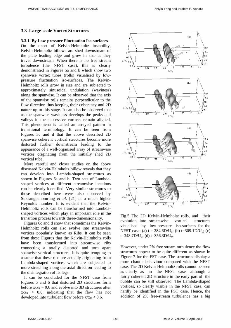
3.3 Large-scale Vortex Structures 3.3.1. By Low-pressure Fluctuation Iso-surfaces On the onset of Kelvin-Helmholtz instability, Kelvin-Helmholtz billows are shed downstream of the plate leading edge and grow in size as they travel downstream. When there is no free stream turbulence (the NFST case), this is clearly demonstrated in Figures 5a and b which show two spanwise vortex tubes (rolls) visualised by low-pressure fluctuation iso-surfaces. The Kelvin-Helmholtz rolls grow in size and are subjected to approximately sinusoidal undulation (waviness) along the spanwise. It can be observed that the axis of the spanwise rolls remains perpendicular to the flow direction thus keeping their coherency and 2D nature up to this stage. It can also be observed that as the spanwise waviness develops the peaks and valleys in the successive vortices remain aligned. This phenomena is called an arrayed pattern in transitional terminology. It can be seen from Figures 5c and d that the above described 2D spanwise coherent vortical structures become more distorted further downstream leading to the appearance of a well-organised array of streamwise vortices originating from the initially shed 2D vortical tube. More careful and closer studies on the above discussed Kelvin-Helmholtz billow reveals that they can develop into Lambda-shaped structures as shown in Figures 6a and b. Two sets of Lambda-shaped vortices at different streamwise locations can be clearly identified. Very similar structures to those described here were also observed by Suksangpanomrung et al. [21] at a much higher Reynolds number. It is evident that the Kelvin-Helmholtz rolls can be transformed into Lambda-shaped vortices which play an important role in the transition process towards three-dimensionality. Figures 6c and d show that sometimes the Kelvin-Helmholtz rolls can also evolve into streamwise vortices popularly known as Ribs. It can be seen from these Figures that the Kelvin-Helmholtz rolls have been transformed into streamwise ribs connecting a totally distorted and torn apart spanwise vortical structures. It is quite tempting to assume that these ribs are actually originating from Lambda-shaped vortices which are subjected to more stretching along the axial direction leading to the disintegration of its legs. It can be concluded for the NFST case from Figures 5 and 6 that distorted 2D structures form before x/xR = 0.6 and evolve into 3D structures after x/xR > 0.6, indicating that the flow has not developed into turbulent flow before x/xR < 0.6.

Fig.5 The 2D Kelvin-Helmholtz rolls, and their evolution into streamwise vortical structures visualised by low-pressure iso-surfaces for the NFST case: (a) t = 284.6D/U0; (b) t=309.1D/U0; (c) t=348.7D/U0; (d) t=356.3D/U0. However, under 2% free stream turbulence the flow structures appear to be quite different as shown in Figure 7 for the FST case. The structures display a more chaotic behaviour compared with the NFST case. The 2D Kelvin-Helmholtz rolls cannot be seen as clearly as in the NFST case although a fairly coherent 2D structure in the early part of the bubble can be still observed. The Lambda-shaped vortices, so clearly visible in the NFST case, can hardly be identified in the FST case. Hence, the addition of 2% free-stream turbulence has a big



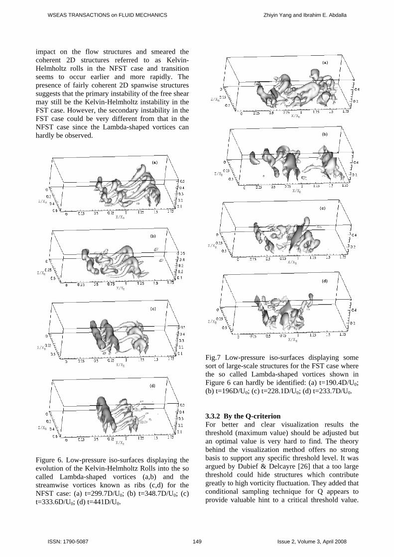
impact on the flow structures and smeared the coherent 2D structures referred to as Kelvin-Helmholtz rolls in the NFST case and transition seems to occur earlier and more rapidly. The presence of fairly coherent 2D spanwise structures suggests that the primary instability of the free shear may still be the Kelvin-Helmholtz instability in the FST case. However, the secondary instability in the FST case could be very different from that in the NFST case since the Lambda-shaped vortices can hardly be observed.

Figure 6. Low-pressure iso-surfaces displaying the evolution of the Kelvin-Helmholtz Rolls into the so called Lambda-shaped vortices (a,b) and the streamwise vortices known as ribs (c,d) for the NFST case: (a) t=299.7D/U0; (b) t=348.7D/U0; (c) t=333.6D/U0; (d) t=441D/U0.

Fig.7 Low-pressure iso-surfaces displaying some sort of large-scale structures for the FST case where the so called Lambda-shaped vortices shown in Figure 6 can hardly be identified: (a) t=190.4D/U0; (b) t=196D/U0; (c) t=228.1D/U0; (d) t=233.7D/U0. 3.3.2 By the Q-criterion For better and clear visualization results the threshold (maximum value) should be adjusted but an optimal value is very hard to find. The theory behind the visualization method offers no strong basis to support any specific threshold level. It was argued by Dubief & Delcayre [26] that a too large threshold could hide structures which contribute greatly to high vorticity fluctuation. They added that conditional sampling technique for Q appears to provide valuable hint to a critical threshold value.



However, as the main issue in vortex visualization is subjectivity, and since this study is not employing any conditional sampling for any variable involved, the threshold in the current simulation is raised to an extent that the 2D spanwise rolls should not appear and as a result of this only structures smaller than the later can be visualized. The Q-criterion is used in the current study to visualise the evolving small scale structures resulting from the breakdown of the 2D Kelvin-Helmholtz rolls. For the NFST case, Figures 8a and b show some kind of well organised streamwise vortical structures by the Q-criterion whereas the previously observed 2D larger Kelvin-Helmholtz rolls by low fluctuating pressure iso-surfaces are not visualised here due to the threshold value chosen, as discussed above. Those structures are usually inclined with a small angle to the axial direction, an indication that they may be formed due to larger structures impinging on the wall. These structures will usually suffer some sort of distortion and even breakdown into smaller structures while passing the transition region. Figures 8c and d show the streamwise vortical structures for the FST case. By comparison, the structures revealed by the Q-criterion for the NFST case are more distinguishable than those appear in the FST case. To be more precise about the word ‘distinguishable’, one can say that the degree of coherency and organisation along both the span and streamwise directions are much obvious in the NFST case compared with the FST case. Furthermore in the NFST case the longitudinal structures are clearly phased along the streamwise direction. In other words, a set of organised longitudinal structures can be observed to evolve in time clearly whereas a lot of interference occurs between the longitudinal structures in the streamwise direction for the FST case. The same conclusion as before can be drawn from the Q-criterion visualisation results that the free stream turbulence speeds up the transition so that the structures are more chaotic. The present study of separated and reattached flow presents several regions with very different characteristics. It is a combination of free-shear and wall flows with recirculation zones. This is a severe test for those two visualization methods and it is evident from the above discussion that low-pressure fluctuation fields can be used to show the structures of larger dimensions better than the structures isolated by the Q-criterion. For a backward-facing step, Delcayre & Lesieur [27] employed the two methods mentioned above. They also found that large-scales structures are represented better by the

low-pressure fluctuation iso-surfaces. The current study is consistent with the previous studies.

Fig.8 Q-isosurfaces showing large-scale structures for both the NFST case (a,b) and the FST case (c,d): (a) t=319.1D/U0; b) t=356.3D/U0; (c) t=194.2D/U0; (d) t=197.9D/U0. 3.3.3 By Vorticity Fields A snapshot of the instantaneous streamwise vorticity iso-surfaces for the NFST case is shown in Figure 9a. The streamwise vorticity field indicates that streamwise vorticity exists in the early stages of the flow development which is not observable in Figures 5, 6 and 7 by the low-pressure fluctuation iso-surfaces. Most strong streamwise vorticity is



confined to the region around the reattachment (x/xR=0.6-1.0). In this region, streamwise vorticity shows some organised structures with some distortion visible in the reattachment region. Strong streamwise vortical structures can be seen stretching in the region between x/xR=1.0-1.4. Such streamwise vortical structures have survived the reattachment region and may travel a considerable distance downstream of reattachment before breaking into smaller scale turbulent structures. This may be the reason why the turbulent boundary layer does not develop into a canonical one up to some distance downstream of reattachment as observed by many researchers [28,29]. Figure 9b shows a snapshot of the instantaneous streamwise vorticity iso-surfaces for the FST case. The main differences are that the streamwise structures in the FST case are not as distinguishable as in the NFST case and the degree of organisation is also reduced.

Fig.9 Streamwise vorticity isosurfaces showing large-scalestructures for both the NFST case (a) and FST case (b): (a)t=365.7.4D/U0; (b) t=199.8D/U0. A snapshot of the instantaneous spanwise vorticity isosurfaces for the NFST case is shown in Figure 10a. It can be seen that a plane sheet of spanwise vorticity starts from the leading edge of the blunt plate and begins to disintegrate at around x/xR=0.6 where 3D motion starts to develop rapidly. Eventually the vorticity sheet breaks down in the region between x/xR=0.5-1.0. Figure 10b presents a snapshot of the instantaneous spanwise vorticity iso-surfaces for the FST case. Similarly a plane sheet of vorticity starts from the leading edge of the blunt plate. However, it begins to disintegrate much

earlier at around x/xR=0.4, breaking down into 3D structures in the region between x/xR=0.4-1.0 more rapidly compared with the NFST case. This can be again confirmed by Figure 3 which shows that in the FST case the predicted axial velocity fluctuations rms values are bigger than those in the NFST case upstream at x/xR = 0.2, 0.4 and 0.6. In the FST case the predicted rms values are smaller than the experimental data at only one very upstream station, x/xR = 0.2, and at x/xR = 0.4 the predicted rms values are very close to the measured turbulent values, supporting the conclusion drawn from the flow visualization on the structures evolution that the distorted 2D structures begin to disintegrate much earlier in the FST case at around x/xR=0.4, breaking down in the region between x/xR=0.4-1.0.

Fig.10 Spanwise vorticity isosurfaces showing large-scale structures for both the NFST case (a) and the FST case (b): (a) t=360D/U0; (b) t=192.3D/U0.

4 Conclusion The transitional flow over a blunt plate held normal to a uniform stream under 0% and 2% free-stream turbulence level has been investigated using LES. The simulated results compare reasonably well with the available experimental data for both cases. The 2% free-stream turbulence level has resulted in 14% reduction in the mean reattachment length compared with the NFST case. This is consistent with most of the experimental work performed on the blunt plate geometry. The transition process leading to breakdown to turbulence and the large-



scale coherent structures at various stages of transition process have been visualised through different visualization methods, the ‘low-pressure’, ‘Q-criterion’ and the ‘vorticity fields’. It has been found that visualization through negative low-pressure fluctuation iso-surfaces seems to show large-scale structures better in comparison with the other two methods. However, Q and vorticity iso-surfaces are better at capturing and revealing relatively small-scale structures. It is clear that large-scale structures are present at different stages in the separated boundary layer transition for both cases but in the FST case they are not as distinguishable as in the NFST case. For the NFST case the Kelvin-Helmholtz rolls grow in size as they travel downstream and are subjected to spanwise waviness which gradually degrades their two-dimensional nature. The streamwise vortices resulting from the transformation of the Kelvin-Helmholtz rolls are noticed to take the form of Lambda-shaped vortices. However, under 2% free-stream turbulence, the 2D Kelvin-Helmholtz rolls are still observable in the early stage but the Lambda-shaped structures can be hardly identified which suggests that the secondary instability at work may be quite different in the FST case. For the FST case, the position of the first unsteadiness moves closer to the separation line and gets strongly amplified at about x/xR=0.25. Generally speaking, the addition of the free-stream turbulence results in increased rate of the randomness of the flow, as expected. Coherency of the early stage structures along the spanwise direction is highly disturbed. References: [1] B.J. Cantwell, Organised Motion in Turbulent Flow, Annual Review of Fluid Mechanics, Vol.13, 1981, pp. 457-515. [2] A.A. Townsend, The Structure of Turbulent Shear Flow, Cambridge University Press, Cambridge, 1956. [3] S. Corrsin, Investigation of Flow in an Axially Symmetric Heated Jet of Air, NACA Adv. Conf. Rep., 3123, 1943. [4] G.L. Brown, A. Roshko, On Density Effects and Large Structure in Turbulent Mixing Layers, Journal of Fluid Mechanics, Vol.64, 1974, pp. 775-816. [5] J. Jeong, F. Hussain, W. Schoppa, J. Kim, Coherent Structure Near the Wall in a Turbulent Channel Flow, Journal of Fluid Mechanics, Vol.332, 1997, pp. 185-214.

[6] A.K.M.F. Hussain, M. Hayakawa M, Education of Large-Scale Organised Structures in a Turbulent Plane Wake, Journal of Fluid Mechanics, Vol.180, 1987, pp. 193-229 [7] A.K.M.F. Hussain, M.V. Melander, Understanding Turbulence via Vortex Dynamics, In the Lumely Symposium: Studies in Turbulence. Springer: Berlin, 1991, pp. 58-178. [8] A.K.M.F. Hussain, Coherent Structures and Turbulence, Journal of Fluid Mechanics, Vol. 173, 1986, pp. 303-356. [9] H. Li, Identification of Coherent Structure in Turbulent Shear Flow with Wavelet Correlation Analysis, Journal of Fluids Engineering, Vol. 120, 1998, pp. 778-785. [10] S.V. Gordeyev, F.O. Thomas, Coherent Structure in the Turbulent Planar Jet, Part 1: Extraction of Proper Orthogonal Decomposition Eigenmodes and Their Self-similarity, Journal of Fluid Mechanics, Vol. 414, 2000, pp. 145-194. [11] P. Comte, J. Silvestrini, P. Begou, Streamwise Vortices in Large-Eddy Simulation of Mixing Layers, European Journal of Mechanics, Vol.17, 1998, pp. 615-637. [12] Z. Yang, Large-Scale Structures at Various Stages of Separated Boundary Layer Transition, International Journal for numerical methods in Fluids, Vol.40, 2002, pp. 723-733. [13] J.C.R Hunt, A.A Wray, P. Moin, Eddies, Stream, and Convergence Zones in Turbulent Flows, Report CTR-S88, centre for turbulence research, 1988. [14] N.J. Cherry, R. Hillier, M.E.M.P. Latour, Unsteady Measurments in a Separating and Reattaching flow, Journal of Fluid Mechanics, Vol.144, 1984, pp. 13-46. [15] K. Sasaki, M. Kiya, Three-Dimensional Vortex Structures in a Leading Edge Separation Bubble at Moderate Reynolds Numbers, Journal of Fluids Engineering, Vol.113, 1991, pp. 405-410. [16] K.S. Hwang, H.J. Sung, M.J. Hyun, Visualization of Large-Scale Vortices in Flow about a Blunt-Faced Flat Plate, Experiments in Fluids, Vol.29, 2000, pp. 198-201. [17] R. Hillier, N.J. Cherry, The Effects of Free Stream Turbulence on Separation Bubbles, Journal of Wind Engineering and Industrial Aerodynamics, Vol.8, 1981, pp. 49-58. [18] M. Kalter, H.H. Fernholz, The Reduction and Elimination of a Closed Separation Region by Free-Stream Turbulence, Journal of Fluid Mechanics, Vol.446, 2001, pp. 271-308. [19] Z. Yang, P.R. Voke, Large-Eddy Simulation of Separated Leading-Edge Flow in General Co-



ordinates, International Journal for Numerical Methods in Engineering, Vol.49, 2000, pp.681-696. [20] Kiya, K. Sasaki, Structure of a Turbulent Separation Bubble, Journal of Fluid Mechanics, Vol.137, 1983, pp. 83-113. [21] A. Suksangpanomrung, N. Djilali, P. Moinat, Large-Sddy Simulation of Separated Flow over a Bluff Rectangular Plate, International Journal of Heat and Fluid Flow, Vol.21, 2000, pp. 655-663. [22] A. Hatziapostolou, K. Krallis, N. G. Orfanoudakis, M. K. Koukou, D. Chatzifotis, G. Raptis, Numerical Prediction of the Flow Field produced by a Laboratory-Scale Combustor: a Preliminary Isothermal Investigation, WSEAS Transactions on Fluid Mechanics, Vol. 1, 2006, pp. 230-235. [23] V. S. Djanali, K.C. Wong, S.W. Armfield, Numerical Simulations of Transition and Separation on a Small Turbine Cascade, WSEAS Transactions on Fluid Mechanics, Vol. 1, 2006, pp. 879-884. [24] Z. Yang, P.R. Voke, Large-Eddy Simulation of Boundary Layer Separation and Transition at a Change of Surface Curvature, Journal of Fluid Mechanics, Vol. 439, 2001, pp. 305-333.

[25] M. Ubaldi, P. Zunino, Transition and Loss Generation in the Profile Boundary Layer of a Turbine Blade, WSEAS Transactions on Fluid Mechanics, Vol. 1, 2006, pp. 779-784. [26] Y. Dubief, F. Delcayre, On Coherent-Vortex Identification in Turbulence. Journal of Turbulence, Vol.1, 2000, pp. 1-22. [27] M. Delcayre, M. Lesieur, Topological Feature in the Reattachment Region of a Backward-Facing Step, AFSOR Int. Conf. On DNS and LES, Ruston, 1997, pp. 1-17. [28] I.P. Castro, E. Epik, Boundary Layer Development after a Separated Region, Journal of Fluid Mechanics, Vol.374, 1998, pp. 91-116. [29] A.E. Alving, H.H. Fernholz, Turbulence Measurements around a Mild Separation Bubble and Downstream of Reattachment, Journal of Fluid Mechanics, Vol.322, 1996, pp. 297-328.



on coherent structures in a separated/reattached flo · on coherent structures in a...

Documents