on ε-biased generators in nc0 - university of california
TRANSCRIPT

On ε-Biased Generators in NC0
Elchanan Mossel∗ Amir Shpilka† Luca Trevisan‡
August 15, 2005
Abstract
Cryan and Miltersen [8] recently considered the question ofwhether there can be a pseudorandom generator inNC0, that is, a pseudorandom generator that mapsn-bit strings tom-bit strings such that every bit of the outputdepends on a constant numberk of bits of the seed.
They show that fork = 3, if m ≥ 4n + 1, there is a distinguisher; in fact, they show that in this case it ispossible to break the generator with alinear test, that is, there is a subset of bits of the output whose XOR has anoticeable bias.
They leave the question open fork ≥ 4. In fact they ask whether every NC0 generator can be broken by astatistical test that simply XORs some bits of the input. Equivalently, is it the case that no NC0 generator cansample anε-biased space with negligibleε?
We give a generator fork = 5 that mapsn bits into cn bits, so that every bit of the output depends on 5 bitsof the seed, and the XOR of every subset of the bits of the output has bias2−Ω(n/c4). For large values ofk, we
construct generators that mapn bits tonΩ(√
k) bits such that every XOR of outputs has bias2−n1
2
√
k .We also present a polynomial-time distinguisher fork = 4, m ≥ 24n having constant distinguishing probability.
For large values ofk we show that a linear distinguisher with a constant distinguishing probability exists oncem ≥ Ω(2kn⌈k/2⌉).
Finally, we consider a variant of the problem where each of the output bits is a degreek polynomial in theinputs. We show there exists a degreek = 2 pseudorandom generator for which the XOR of every subset of theoutputs has bias2−Ω(n) and which mapsn bits toΩ(n2) bits.
1 Introduction
A pseudorandom generator is an efficient deterministic procedure that maps a shorter random input into a longeroutput that is indistinguishable from the uniform distribution by resource-bounded observers.
A formalization of the above informal definition is to consider polynomial-time proceduresG mappingn bits intom(n) > n bits such that for every propertyP computable by a family of polynomial-size circuits we have that thequantity
∣
∣
∣
∣
Prz∈0,1m(n)
[P (z) = 1] − Prx∈0,1n
[P (G(x))]
∣
∣
∣
∣
∗Department of Statistics, U.C. Berkeley, CA 94720-3869. Email: [email protected]. Supported by a Miller fellowshipin Statistics and Computer Science, by a Sloan fellowship inMathematics and by NSF grant DMS-0504245
†Department of Computer Science and Applied Mathematics, Weizmann Institute of Science, Rehovot, Israel. Email:[email protected]. Supported by National Security Agency (NSA) and Advanced Research and Development Activ-ity (ARDA) under Research Office (ARO) contract no. DAAD19-01-1-0506, and by the Koshland fellowship.
‡Computer Science Division, U.C. Berkeley, CA 94720-1776. Email: [email protected]. Supported by NSF Grant CCR-9984783/CCR-0406156, US-Israel BSF grant 2002246, a SloanResearch Fellowship and an Okawa Foundation Grant.
1

goes to zero faster than any inverse polynomial inn. The existence of such a procedureG is equivalent to the existenceof one-way functions [15], pseudorandom functions [11] andpseudorandom permutations [23].
What are the minimal computational requirements needed to compute a pseudorandom generator? Linial et al.[20] prove that pseudorandom functions cannot be computed in AC0 (constant-depth circuits with NOT gates andunbounded fan-in AND and OR gates). To be precise, the results in [20] only rule out security against adversariesrunning in timeO(n(log n)O(1)
). Their result does not rule out the possibility that pseudorandom generators couldbe computed in AC0, since the transformation of pseudorandom generators intopseudorandom functions does notpreserve bounded-depth.
Kharitonov [19] shows that a pseudorandom generator with superlinear stretch can be computed in NC1, that is, itcan be computed by a circuit of polynomial size, logarithmicdepth, and gates of constant fan-in. (It is known that NC1
properly contains AC0.) Impagliazzo and Naor [17] present a candidate pseudorandom generator in AC0. Goldreich[12] suggests a candidate one-way function in NC0. Recall that NC0 is the class of functions computed by bounded-depth circuits with NOT gates and bounded fan-in AND and OR gates. In an NC0 function, every bit of the outputdepends on a constant number of bits of the inputs. While it iseasy to see that there can be no one-way function suchthat every bit of the output depends on only two bits of the input (as finding an inverse can be formulated as a 2SATproblem) it still remains open whether there can be a one-wayfunction such that every bit of the output depends ononly three bits of the input. Applebaumet al. [1] have very recently provided evidence that such one-way functionsexist.
Cryan and Miltersen [8] consider the question of whether there can be pseudorandom generators in NC0, that is,whether there can be a pseudorandom generator such that every bit of the output depends only on a constantk numberof bits of the input. They present a distinguisher in the casek = 3, m > 4n, and they observe that their distinguisheris a linear distinguisher, that is, it simply XORs a subset of the bits ofthe output. Cryan and Miltersen ask whetherthere is any pseudorandom generator in NC0 whenm is superlinear inn. Specifically, they ask whether the followingis the case: that for every constantk, and for every generator for whichm is super-linear inn and for which everyoutput bit depends on at mostk bits of the input, a linear distinguisher exists.
In order to formulate an equivalent version of this problem,we introduce the notion of aε-biaseddistribution.
Definition 1. For ε > 0, we say that a random variableX = (X1, . . . , Xm) ranging over0, 1m is ε-biased if forevery subsetS ⊆ [m] we have1/2 − ε ≤ Pr[
⊕
i∈S Xi = 0] ≤ 1/2 + ε.
It is known [27, 3] that anε-biased distribution can be sampled by using onlyO(log(m/ε)) random bits, which istight up to the constant in the big-Oh.
The problem of [8] can therefore be formulated by asking whether there exists anyε-biased generator in NC0 thatsamples anm-bit ε-biased distribution starting from, say,o(m) random bits and a negligibleε.
Our Results
We first extend the result of Cryan and Miltersen by giving a (non linear) distinguisher for the casek = 4, m ≥ 24n.
Theorem 2. LetG = (g1, . . . , gm) : 0, 1n → 0, 1m be a map such that eachgi depends on at most4 coordinatesof the input andm ≥ 24n. Then there exists a polynomial time algorithm which distinguishes betweenG and arandom string with constant distinguishing probability. More precisely, the algorithm will output “yes” for the outputof the generatorG with probabilityΩ(1), and for a random string with probabilitye−Ω(m).
Our distinguisher has a constant distinguishing probability, which we show to be impossible to achieve with lineardistinguishers. Our distinguisher uses semidefinite programming and uses an idea similar to the “correlation attacks”used in practice against stream ciphers.
2

For allk, it is trivial that a distinguisher exists form ≥ 22k(nk
)
(the number of functions onk bits), and it is easyto see that a distinguisher exist whenm ≥ k
(
nk
)
(as there is a linear dependence among the output bits in thiscase).We show using a duality lemma proven in [25] that in fact, a distinguisher with a constant distinguishing probabilityexists oncem ≥ Ω(2kn⌈k/2⌉) by proving
Theorem 3. For every integer0 < k and any0 < ε < 2−2k−1, if G = (g1, . . . , gm) is anε-biased pseudorandomgenerator, where each of thegi’s depend on at mostk bits, then
m ≤⌈ k
2⌉
∑
t=0
(
n
t
)
22(k−t) ≤ k22k
(
n
⌈k2⌉
)
.
Then we present anε-biased generator mappingn bits intocn bits such thatε = 1/2Ω(n/c4) and every bit of theoutput depends only onk = 5 bits of the seed, i.e., we prove
Theorem 4. For everyc and sufficiently largen, there is a generator inNC05 mappingn bits intocn bits and sampling
anε-biased distribution, whereε = 2−n/O(c4).
The main idea in the construction is to develop a generator with k = 3 that handles well linear tests that XOR asmallnumber of bits, and then develop a generator withk = 2 that handles well linear tests that XOR alargenumberof bits. The final generator outputs the bitwise XOR of the outputs of the two generators, on two independent seeds.
The generator uses a kind of unique-neighbor expander graphs that are shown to exist using the probabilisticmethod, but that are not known to be efficiently constructible, so the generator is in NC0 but not inuniformNC0.
Later we present similar constructions for large values ofk. We writef(n, k) = Ok(g(n)) if f(n, k) ≤ h(k)g(n)for some functionh; similarly we will use the notationok.
Theorem 5. Letk be a positive integer. There exists anε-biased generator inNC0k fromn bits to
(
n√k − 6
)
√k
2−3
= n√
k( 12−ok(1))
bits whose bias,ε, is at most
exp
(
− n1
2√
k
4 × 2√
k
)
.
Note the gap for large values ofk between our constructions that outputn(√
k/2)(1−ok(1)) bits, and the boundsshowing a distinguisher exists for generators that outputn(k/2)(1+ok(1)) bits.
Finally, we begin a study of the question of whether there arepseudorandom generators with superlinear stretchsuch that each bit of the output is a function of the seed expressible as a degree-k polynomial overGF (2), wherek isa constant. This is a generalization of the main question addressed in this paper, since a function depending on onlykinputs can always be expressed as a degree-k polynomial. Furthermore, low-degree polynomials are a standard classof “low complexity” functions from an algebraic perspective. In ourNC0
5 construction of anε-biased generator withexponentially smallε and superlinear stretch, every bit of the output is a degree-2 polynomial. We show that
Theorem 6. ∀1 ≤ m ≤ n there exists anε-biased generatorG = (g1, ..., gt) : 0, 1n 7→ 0, 1t, t = ⌊n2 ⌋ · m, such
thatgi is a degree2 polynomial, and the bias of any non trivial linear combination of thegi’s is at most2−n−2m
4 .
3

Later Results and Open Questions
Applebaumet al. [1] have recently made substantial progress on the main questions left open by our work about thecasesk = 3, 4.
In the casek = 3, Applebaumet al. [1] present a construction of anε-biased generator withm = (1 + α) · n,whereα > 0 is an absolute constant. They also show that under relatively general assumptions, there are one-wayfunctions such that every bit of the output depends on only 3 bits of the input.
In the casek = 4, Applebaumet al. [1] present a construction of a pseudorandom generator withm = n + nα,whereα can be chosen to be any constant smaller than 1. The generatoris secure under the assumption that thereexists pseudorandom generators in
⊕
L/poly, which is a fairly general assumption.
It remains open whether a cryptographically strong generator can be realized in the casek = 3, whether a cryp-tographically strong generator with linear stretch can be realized in the casek = 4, and whether a cryptographicallystrong generator with superlinear stretch can be realized in the casek = 5.
Another important open problem which may be more accessibleis to understand the right asymptotic forε-biasedgenerators for largek. It is tempting to conjecture that either the upper boundnO(k) or the lower boundnΩ(
√k) is
actually tight.
Organization
In section 2 we review the analysis for the casek = 3 of [8]. In section 3 we give a distinguisher for the casek = 4.In section 4 we prove an upper bound on the length of the outputof anε-biased generator inNC0
k.
In section 5 we construct anε-biased generator for the casesk = 4, 5. The results for largerk are discussed insection 6. In section 7 we explicitly construct anε-biased generator such that every bit of the output is a polynomialof degree2.
An extended abstract reporting on the results here appearedin [26].
2 Review of the Casek = 3
In this section we summarize the main result of [8]. We also generalize some of the arguments of [8] that are neededfor our results.
2.1 Preliminaries
We say that a functiong : 0, 1n → 0, 1 is balancedif Prx
[g(x) = 1] = 1/2. We say that a functiong : 0, 1n →0, 1 is unbiasedtowards a functionf : 0, 1n → 0, 1 if Pr
x[g(x) = f(x)] = 1/2, and that it isbiased towards
f (or correlatedwith f ) otherwise. A functiong : 0, 1n → 0, 1 is affineif there are valuesa0, . . . , an ∈ 0, 1such thatg(x1, . . . , xn) = a0 ⊕ a1x1 ⊕ . . . ⊕ anxn, it is non-affineotherwise.
The following lemma was proved by case analysis fork = 3 in [8], and the casek = 4 could also be derived froma case analysis appearing in [8] (but it is not explicitly stated). The proof of the general case follows using the Fourierrepresentation of boolean functions.
The Fourier representation is easier to work with when considering functions from±1n → ±1. For a booleanfunctionf : 0, 1k → 0, 1 we writeF for the functionF : ±1k → ±1 defined as
F ((−1)x1 , . . . , (−1)xk) = (−1)f(x1,...,xk). (1)
4

For the boolean functionsf, g, h discussed in this section, the functionsF, G, H will be the corresponding mappingsto ±1. For a setS ⊆ [k], we letUS : ±1k → ±1 be defined asUS(X) =
∏
i∈S Xi, that isUS is the charactercorresponding toS. It is well known thatUSS⊆[k] is an orthonormal basis for the space of functions from±1k toR with respect to the inner product
< F, G >=1
2k
∑
x∈0,1k
F (x) · G(x).
We writeF (X) =∑
S F (S)US(X) for the representation ofF in the basisUS. Because of orthonormality, thecoefficientsF (S) satisfy the relationF =< F, US >.
Note that iff, g are boolean functions andF, G are defined as in (1), thenPr[f(x) = g(x)] = Pr[F (x) =G(x)] = 1/2 + 1/2 < F, G >. In particular,f andg are correlated if and only if< F, G >6= 0.
Lemma 7. Letg : 0, 1n → 0, 1 be a non-affine function that depends on onlyk variables. Then
• There exists an affine function on at mostk − 2 variables that is correlated withg.
• Let l be the affine function that is biased towardsg and that depends on a minimal number of variables. That is,for somed, l depends ond variables,Pr
x[g(x) = l(x)] > 1/2, andg is unbiased towards affine functions that
depend on less thand variables.
ThenPrx
[g(x) = l(x)] ≥ 1/2 + 2d−k.
Proof. • Let f : 0, 1k → 0, 1 be a non-affine function. We prove that there exists a setS of size at mostk − 2 such thatF (S) 6= 0. This implies thatF is correlated withUS and therefore thatf is correlated with⊕i∈Sxi as needed.
Look at the functionh(x1, . . . , xk) = f(x1, . . . , xk) ⊕ ⊕ki=1xi. Sincef is non-affine,h is not a constant
function. LetH be the±1 representation ofh. As the±1 representation of⊕ki=1xi is U[k], we get thatH
has the Fourier representation
H = U[k] · F = U[k] ·∑
S⊆[k]
F (S)US =∑
S⊆[k]
F (S)U[k]\S =∑
S
F ([k] \ S)US .
It therefore suffices to prove thatU[k] · F has a coefficientF (S) 6= 0 with |S| ≥ 2. We will prove that anyfunction which depends on more than one bit, has a non-zero coefficient with |S| ≥ 2. This will prove the firstpart, since ifh depends on at most one bit thenf is affine.
Indeed, assume the contradictionF = a0 +
∑
i
aiUi
For a± vectorX, writeX i for the vector where thei’th coordinate ofX is multiplied by−1. Note that for alliand allX, it holds that2ai = F (X)−F (X i) ∈ 0,±2, which implies thatai ∈ 0,±1. Parseval’s inequalityimplies that
∑
a2i = 1. We therefore conclude thatF (X) depends on one bit as needed. This completes the
proof of the first claim.
• Note thatf is correlated with⊕i∈Sxi if and only if F (S) 6= 0. Moreover,
Pr[f(x) = ⊕i∈Sxi] =1 + F (S)
2.
5

The claim will therefore follow once we prove that ifF =∑
|S|≥d F (S)US , andF (S) 6= 0 for a setS of size
d, then|F (S)| ≥ 2d+1−k.
By looking atU[k]F instead ofF , it suffices to prove that if
F =∑
|S|≤k−d
F (S)US , (2)
andS′ is a set of sizek−d such thatF (S′) 6= 0, then|F (S′)| ≥ 2d−k+1. In order to prove the last claim, define
A(X) =∑
T⊆S′
(−1)|T |F (XT ) =∑
T⊆S′
(−1)|T | ∑
S⊆[k]
F (S)US(XT ) =∑
S⊆[k]
F (S)∑
T⊆S′
(−1)|T |US(XT ),
whereXT is X where the coordinates atT are flipped (multiplied by−1). It is then clear thatA obtains aneveninteger value in the interval[−2k−d, 2k−d].
On the other hand, ifS does not containS′ andj ∈ S′ \ S, then for allX
∑
T⊆S′
(−1)|T |US(XT ) =∑
T⊆S′,j /∈T
(−1)|T |US(XT ) +∑
T⊆S′,j∈T
(−1)|T |US(XT )
=∑
T⊆S′,j /∈T
US(XT )((−1)|T | + (−1)|T |+1) = 0.
SinceF (S) = 0 for all S strictly containingS′, it follows that
A(X) = F (S′)∑
T⊆S′
(−1)|T |uS′(XT ) = 2k−dF (S′)uS′(X).
We therefore conclude thatF (S′) is of the form 2i2k−d , for some integeri ∈ [−2k−d−1, 2k−d−1]. In particular,
sinceF (S′) 6= 0, it follows that|F (S′)| ≥ 2−d+k+1 as needed.
For example, fork = 3, a non-affine functiong is either unbalanced, or it is biased towards one of its inputs; inthe latter case it agrees with an input bit (or with its complement) with probability at least3/4.
Fork = 4, a functiong either is affine, or it is unbalanced, or it has agreement at least5/8 with an affine functionthat depends on only one input bit, or it has agreement at least 3/4 with an affine function that depends on only twoinput bits.
2.2 The Casek = 3
Let G : 0, 1n → 0, 1m be a generator and letgi : 0, 1n → 0, 1 be thei-th bit of the output of the generator.Suppose eachgi depends on only three bits of the input.
Suppose that one of thegi is not a balanced function. Then we immediately have a distinguisher.
Suppose that more thann of thegi are affine. Then one of them is linearly dependent on the others, and we alsohave a distinguisher.
It remains to consider the case where at leastm − n of the functionsgi are balanced and not affine. LetI be theset of i for which gi is as above. Then, by lemma 7, for each suchgi there is a affine functionli that depends on
6

only onebit, such thatgi agrees withli on a3/4 fraction of the inputs. By replacinggi with gi ⊕ 1 when needed,we may assume that each suchgi has correlation at least3/4 with one of the bits of its input. The following lemmanow implies a constant distinguishing probability oncem ≥ 4n + 1. While the above analysis uses the same ideas asin [8], it is slightly better because we achieve constant bias instead of inverse polynomial bias. We first prove a verygeneral lemma that will be also used in later sections, and then we derive the conclusion that we need for the case ofk = 3.
Lemma 8. For everyδ > 0 there are constantscδ ≤ ⌈ 1δ2 ⌉ − 1 ≤ 1
δ2 and εδ ≥ 3δ2
4 such that the following holds.Let G : 0, 1n → 0, 1m, and letG(x) = (g1(x), . . . , gm(x)). LetL be a set of functions and suppose that eachfunctiongi(x) agrees with an element ofL or with its complement with probability at least1/2 + δ. In other words,for everygi there existsf ∈ L such that
Prx
[gi(x) = f(x)] ≥ 1
2+ δ or
Prx
[gi(x) 6= f(x)] ≥ 1
2+ δ.
Assume thatm ≥ 1 + cδ|L|. Then there arei 6= j such thatgi ⊕ gj has bias at leastεδ. Moreover,c1/4 ≤ 3 andc1/8 ≤ 9.
Proof. By the pigeonhole principle there is a functionf ∈ L and a set of indicesC ⊆ [m], such that|C| ≥ ⌈ m|L|⌉,
and for everyi ∈ C, gi or 1 − gi is correlated withf . Assume w.l.o.g. that for everyi ∈ C, gi is correlated withf(otherwise replacegi with 1 − gi).
Define the random variable
Z(x) = |# i ∈ C : gi(x) = 0 − # i ∈ C : gi(x) = 1 |.
Consider the expectation ofZ(x) (wherex is uniformly chosen from0, 1n). We have that
E[Z(x)] = E [|# i ∈ C : gi(x) = f(x) − # i ∈ C : gi(x) 6= f(x)|]
≥ E [# i ∈ C : gi(x) = f(x)] − E [# i ∈ C : gi(x) 6= f(x)] ≥ |C| ·((
1
2+ δ
)
−(
1
2− δ
))
= 2δ|C|.
Note that the average value ofZ over the uniform distribution isO(√
|C|). We conclude that for|C| = αδ−2, fora sufficiently largeα, the difference of expected values ofZ under the generator and under the uniform distributionis Ω(|C|δ). This implies that the statistical distance between the output of the generator and the uniform distributionover |C| bits isΩ(δ). By the Vazirani XOR lemma [31] (see [10] for an excellent exposition of the XOR lemma), italso follows that the XOR of some subset of the bits ofC has biasΩ(δ2−|C|) = 2−O(δ−2). However we would like toobtain a better dependence betweenδ andε.
For i, j ∈ C defineZi,j(x) to be1 if gi(x) = gj(x) and−1 otherwise. Note thatE[Zi,j ] equals twice the bias ofgi ⊕ gj . ClearlyZi,i = 1. We have thatZ(x)2 =
∑
i,j Zi,j . In particular we get that
E
∑
i,j
Zi,j(x)
= E[
Z(x)2]
≥ E[Z(x)]2 ≥ 4δ2|C|2.
Hence for|C| = ⌈ 1δ2 ⌉ we get that
E
∑
i,j
Zi,j(x)
≥ 4|C|.
7

As E[∑
i Zi,i] = |C|, it follows thatE[∑
i6=j Zi,j ] ≥ 3|C|, and so there must bei 6= j ∈ C such that
E[Zi,j ] ≥3|C|
|C| · (|C| − 1)≥ 3δ2
2.
In other words,gi ⊕ gj has a3δ2
4 bias. Thus takingm = 1 + |L| · (⌈ 1δ2 ⌉ − 1) we obtaincδ = ⌈ 1
δ2 ⌉ − 1.
We now consider two special cases.
Let |C| = 4, δ = 14 . By the above argument we get thatE[Z(x)] ≥ 2 × 1
4 × |C| = 2. On the other hand, for theuniform distribution on4 bits the average ofZ(x) is
2
16
(
2 ×(
4
1
)
+ 4 ×(
4
0
))
=3
2< 2 = 2.
Thus, if |C| = 4 we get by Vazirani’s XOR lemma that some subset of thegi’s has some constant bias, so we can setc1/4 = 3.
Similarly, when|C| = 10 the average ofZ(x) for the uniform distribution is
2
210
4∑
i=0
(10 − 2i)
(
10
i
)
=2520
1024< 2 × 1
8· 10,
so we can setc1/8 = 9.
To conclude the case ofk = 3 we note that ifm ≥ 1+4n, and the output of the generator contains at mostn affinefunctions then at least1 + 3n output bits that are not affine and so we can apply Lemma 8, where L = π1, . . . , πnis the set ofn “projection” functionsπi() such thatπi(x1, . . . , xn) = xi. The consequence of Lemma 8 is that two ofthe output bits are correlated.
3 Distinguisher for the Casek = 4
In this section we construct a distinguisher fork = 4. We restate Theorem 2.
Theorem. LetG = (g1, . . . , gm) : 0, 1n → 0, 1m be a map such that eachgi depends on at most4 coordinates ofthe input andm ≥ 24n. Then there exists a polynomial time algorithm which distinguishes betweenG and a randomstring with constant distinguishing probability. More precisely, the algorithm will output “yes” for the output of thegeneratorG with probabilityΩ(1), and for a random string with probabilitye−Ω(m).
• The first case we consider is where there are more than0.001m of the gi that are unbalanced. Suppose thatg1, . . . , gp are unbalanced andp ≥ 0.001m. Then there exist fixed bitsb1, . . . , bp such thatPr[gi = bi] ≥ 9/16.Thus by Markov’s inequality:
Prz∈0,1n
[ | i | gi(z) = bi)|p
≥ 17
32
]
≥ 1
32.
On the other hand, ifr1, . . . , rp are chosen uniformly at random, then
Pr
[ | i | ri = bi)|p
≥ 17
32
]
≤ e−Ω(m)
by Chernoff’s inequality.
8

• The second case is where more thann + 0.001m of thegi are linear. In this case we can write at least0.001mindependent linear combinations in the output bits of the generator that hold with probability1. The probabilitythat these combinations hold for truly random bits is2−0.001m. Thus the statement of the theorem follows inthis case as well.
• If one of thegi is biased towards one of the bits of its input, then it followsfrom Lemma 7 that it must agreewith that bit or its complement with probability at least5/8. Suppose that more thanc1/8n = 9n + 0.001m ofthe functionsgi have bias towards one bit. Then by the proof of Lemma 8, there exists at leastp ≥ 0.0001mdisjoint setsS1, . . . , Sp of thegi’s such that|Sr| ≤ 10 and⊕i∈Srgi has bias at least2−10 bias towards a constantbit br for all 1 ≤ r ≤ p. Thus, as in the first case,
Prz∈0,1n
[ | r | ⊕i∈Sr gi(z) = br)|p
≥ 1
2+ 2−11
]
≥ 2−11
and from Chernoff’s bound it follows that ifri are truly random then
Pr
[ | r | ⊕i∈Sr ri = br|p
≥ 1
2+ 2−11
]
≤ e−Ω(m).
Thus, the proof follows in this case as well.
• It remains to consider the case where at least0.997m − 10n of the functions are balanced, non-linear, andunbiased towards single bits. Following [8], we call such functionsproblematic. It follows from Lemma 7 thatfor each problematicg there is an affine functionl of two variables that agrees withg on a3/4 fraction of theinputs. Again, by replacinggi by gi ⊕ 1, when needed, we may assume that all the problematicg′is have3/4agreement probability with some linear function.
Let P be the set ofi such thatgi is problematic. For each suchi we denote byli the linear function of twoinputs that agrees withgi on a3/4 fraction of the inputs. In the next section we show how ifp = |P | ≥0.997m − 10n ≥ 13.9n, then one can “break” the generator using correlation attack. Correlation attacks areoften used in practice to break pseudorandom generators. The distinguisher below is an interesting examplewhere one can actually prove that correlation attack results in a polynomial time distinguisher.
3.1 The Distinguisher Based on Semidefinite Programming
Given a string(r1, . . . , rp) ∈ 0, 1p, consider the following linear system overGF (2) with two variables per equa-tion.
∀i ∈ P li(x) = ri. (3)
We will argue that the fraction of satisfied equations in the system (3) is distributed differently ifr1, . . . , rp isuniform or if it is the output ofG. Since the expected number of equations (3) satisfied whenri = gi is at least3p/4,it follows by Markov’s inequality that
Lemma 9. If r1, . . . , rp are the output ofg1, . . . , gp, respectively (where thegi’s are problematic), then, for everyε > 0, there is a probability of at leastε that at least3/4 − ε fraction of the equations in (3) are satisfiable. Moreformally
Prz∈0,1n
[ | i | gi(z) = ℓi(z))|p
≥ 3
4− ε
]
≥ ε.
9

Lemma 10. If r1, . . . , rp are chosen uniformly at random from0, 1p, and p > (1/2δ2)(ln 2)(n + c), then theprobability that there is an assignment that satisfies more than a1/2 + δ fraction of the equations of (3) is at most2−c.
Proof. Fix an assignmentz; then, by Chernoff’s inequality, the probability that a fraction at least1/2 + δ of theri agree withli(z) is at moste−2δ2p ≤ 2−c−n. By a union bound, there is at most a probability2−c that such azexists.
Given a system of linear equations overGF (2) with two variables per equation, it is NP-hard to determine thelargest number of equations that can be satisfied, but the problem can be approximated to within a.878 factor usingsemidefinite programming [13]. We now prove theorem 2.
Proof of Theorem 2: Let δ = .158, ε = 10−4. Thus,.878(3/4− ε) > 1/2+ δ. The statement of the theorem followsfrom the previous arguments unless there arep problematic functions wherep > 0.997m − 10n. Given a string(r1, ..., rp), which is either random in0, 1p or from the distributionG(z) restricted to problematic functions (wherez is random), we consider the system (3). Using semidefinite programming [13] we get a polynomial time algorithmthat is successful if a3/4 − ε fraction of the equations hold, and fails if no more than0.878(3/4 − ε) > 1/2 + δ ofthe equations hold. Letc = 0.0005n. By lemma 10 ifp > 13.89n > (1/2δ2)(ln 2)(n + c), then the probability thatmore than1/2 + δ of the equations are satisfied, whenr1, ..., rp are chosen randomly, is at most2−c = exp(−Ω(n)).On the other hand, when(r1, ..., rp) is taken from the generator then the probability that at least 3/4 − ε fraction ofthe equations are satisfied is at leastε. The theorem follows.
3.2 Correlation Attacks
In this section we discuss how our distinguisher for the casek = 4 can be seen as a “correlation attack.”
Correlation attacks are a class of attacks that are often attempted in practice against candidate pseudorandomgenerators. Pseudorandom generators are called “stream ciphers” in the applied cryptography literature, see e.g. theintroduction of [18] for an overview.
The basic idea is as follows. Given a candidate generatorG : 0, 1n → 0, 1m, whereG(x) = g1(x), . . . , gm(x),we first try and find linear relations between input bits and output bits that are satisfied with non-trivial probability.For example, suppose we find coefficientsai,j , bi,j andcj such that each of the equations
∑ni=1 ai,1xi +
∑mi=1 bi,1gi(x) = c1 (mod 2)
∑ni=1 ai,2xi +
∑mi=1 bi,2gi(x) = c2 (mod 2)
. . .∑n
i=1 ai,txi +∑m
i=1 bi,tgi(x) = ct (mod 2)
(4)
is satisfied with probability bounded away from 1/2.
Now we want to use this system of equations in order to build a distinguisher. The distinguisher is given a samplez = (z1, . . . , zm) and has to decide whetherz is uniform or is the output ofG. The distinguisher substituteszi inplace ofgi(x) in (4) and then tries to find anx that maximizes the number of satisfied equations. The hope isthat, ifz = G(x), then we will findx as a solution of the optimization problem.
Unfortunately, maximizing the number of satisfied equations in a linear system overGF (2) is an NP-hard problem,and, in fact, it is NP-hard to achieve an approximation factor better than 1/2 [14]. In practice, one uses belief-propagation algorithms that often work, although the method is typically not amenable to a formal analysis.
10

In Section 3.1, we were able to derive a formal analysis of a related method because we ended up with a systemof equations having only two variables per equation, a classof instances for which good approximation algorithmsare known. Furthermore, we did not try to argue that, when themethod is applied to the output of the generator, weare likely to recover the seed; instead, we argued that just being able to approximate the largest fraction of satisfiableequations gives a way to distinguish samples of the generators from random strings.
4 O(nk/2) upper bound
In this section we prove the following theorem which gives anupper bound on the maximal stretch of anε-biasedgenerator in NC0k. We restate Theorem 3.
Theorem. For every integer0 < k ≤ n and any0 ≤ ε < 2−2k−1, if G = (g1, . . . , gm) is anε-biased pseudorandomgenerator, where each of thegi’s depend on at mostk bits, then
m ≤⌈ k
2⌉
∑
t=0
(
n
t
)
22(k−t) ≤ k22k
(
n
⌈k2⌉
)
. (5)
The proof uses the following lemma from [25].
Lemma 11 ([25]). Letf : 0, 1k → 0, 1 then for allr
• Eitherf is a polynomial of degree at mostr overGF (2), or
• f is biased towards an affine function of at mostk − r variables.
Proof of Theorem 3: For 0 ≤ t ≤ n, write B(t) =∑t
i=0
(ni
)
. Sets = ⌊k/2⌋, r = k − s. By Lemma 11 everygi
is either a degree≤ r polynomial, or is biased towards an affine function of at mosts variables. Letp be the numberof degree≤ r polynomials among thegi’s, andbt be the number ofgi’s biased towards an affine function of exactlytvariables (but not towards an affine function with less thant variables). Clearly,m ≤ p+
∑st=0 bt. Note that theB(r)
monomials of degree≤ r on the variablesx1, . . . , xn form a basis for the vector space of all degree≤ r polynomialsin x1, . . . , xn. Therefore ifp > B(r), there is a linear dependency between theg′is. We therefore conclude that
p ≤ B(r). (6)
On the other hand, note that by Lemma 7, ifg is biased towards an affine function oft ≤ s variables (but nottowards an affine function with less thant variables) then there exists an affine functionℓ of t variables such thatPr[g = ℓ] ≥ 1/2 + 2t−k. Moreover, there are exactly
(
nt
)
linear functions ont variables. Fort ≤ s let Lt be the setof linear functions ont variables. Lemma 8 implies that if
bt ≥ 1 + |Lt| · c2t−k = 1 +
(
n
t
)
·(
22(k−t) − 1)
then there is a⊕ of two of thegi’s that has at least a3422t−2k > 2−2k−1 bias. It therefore follows that
bt ≤(
n
t
)
(22(k−t) − 1). (7)
Combining (7) and (6) we obtain that
m ≤ B(r) +
⌊ k2⌋
∑
t=0
(
n
t
)
(22(k−t) − 1) ≤⌈ k
2⌉
∑
t=0
(
n
t
)
22(k−t) ≤ k22k
(
n
⌈k2⌉
)
11

as needed.
5 Constructions for k = 5 and k = 4
5.1 Overview
In this section we prove Theorem 4. We will also give a construction of ak = 4 generator with inverse-polynomialbias. In both cases, we will construct a generator mapping2n bits into cn bits. It is helpful to think ofc as a largeconstant, although the results fork = 5 hold also ifc is a function ofn.
We will construct two generators: one will be good against linear tests that involve a small number of output bits(we call themsmall tests), and another is good against linear tests that involve a large number of output bits (we callthem large tests). The final generator will be obtained by computing the two generators on independent seeds, andthen XOR-ing their output bit by bit. In this way, we fool every possible test.
The generator that is good against large tests is such that every bit of the output is just the product of two bitsof the seed. We argue that the sum (modulo 2) oft output bits of the generator has bias exponentially small int/c2,wherec, as above, is the stretch of the generator.
Then we describe a generator that completely fools linear tests of size up to aboutn/c2, and such that every bit ofthe output is the sum of three bits of the seed. Combined with the generator for large tests, we get a generator in NC0
5
such that every linear test has bias2−O(n/c4).
5.2 The Generator for Large Tests
Let us call the bits of the seedy1, . . . , yn.
Let K be an undirected graph formed byn/(2c + 1) disjoint cliques each with2c + 1 vertices (we assume forsimplicity thatn/(2c + 1) is an integer).K hasn vertices that we identify with the elements of[n]. K hascn = medges. Fix some ordering of the edges ofK, and let(aj, bj) be thej-th edge ofK. Define the functionsq1, . . . , qm asqj(y1, . . . , yn) = yaj
ybj.
Lemma 12. For every subsetS ⊆ [m], the functionqS(y) =∑
j∈S qj(y) is such that
|Pry
[qS(y) = 0] − 1
2| ≤
(
1
2
)1+|S|/(2c2+c)
.
The proof relies on the following two standard lemmas. The first one from [8] is a special case of the Schwartz-Zippel lemma [29, 32].
Lemma 13 ([8]). Letp be a non-constant degree-2 multilinear polynomial overGF (2). Then1/4 ≤ Pr[p(x) = 0] ≤3/4.
It is well known and easy to prove by induction that
Lemma 14. LetX1, . . . , Xt be independent 0/1 random variables, and suppose that for everyi we haveδ ≤ Pr[Xi =0] ≤ 1 − δ. Then
1
2− 1
2(1 − 2δ)t ≤ Pr
[
⊕
i
Xi = 0
]
≤ 1
2+
1
2(1 − 2δ)t.
12

We can now prove lemma 12.
Proof of Lemma 12.: We can think ofS as a subset of the edges ofK. Each connected component ofK has2c2 + cedges, soS contains edges coming from at least|S|/(2c2 + c) different connected components. Lett be the numberof connected components. If we decompose the summation
∑
j∈S qj(y1, . . . , yn) into terms depending on each of theconnected components, then each term is a non-trivial degree-2 polynomial, and thet terms are independent randomvariables wheny1, . . . , yn are picked at random. We can then apply lemma 14, where theXi are the values taken byeach of thet terms in the summation,δ = 1/4, andt ≥ |S|/(2c2 + c).
In particular it follows that if we defineG1(y1, ..., yn) = (q1, ..., qm) then any linear combination of at leastΩ(n)coordinates of the output ofG has an exponentially small bias.
5.3 The Generator for Small Tests
Let A ∈ 0, 1n×m be a matrix such that every row is a vector in0, 1n with exactly three non-zero entries, and alsoassume that every set ofσ − 1 rows ofA is linearly independent. LetA1, . . . , Am be the rows ofA. We define thelinear functionsl1, . . . , lm asli(x) = Ai · x. Note that each of these linear functions depends on only three bits of theinput.
Proposition 15. For every subsetS ⊆ [m], |S| < σ, the functionlS(x) =∑
j∈S lj(x) is balanced.
Proof. We havelS(x) = (∑
j∈S Aj) ·x, and since∑
j∈S Aj is a non-zero element of0, 1n (asAii∈S are linearlyindependent), it follows thatlS() is a non-trivial linear function, and therefore it is balanced.
Lemma 16. For everyc = c(n) = o(√
n/(log n)3/4) and for sufficiently largen there is a 0/1 matrixA with cnrows andn columns such that every row has exactly three non-zero entries and such that every set ofσ − 1 =n/(4e2c2(n)) − 1 rows are linearly independent.
Proof. We shall construct the matrixA as the adjacency matrix of a bi-partite expander graph. We begin by showinga relation between an expansion of bi-partite graphs and linear independence of related linear functions.
Let G = (L, R, E) be a bi-partite graph such that|R| = n. G has theb - right unique neighborproperty, if forany setV ⊆ L, |V | ≤ b there exists a vertexu ∈ R such that|N(u) ∩ V | = 1. Assign then input variables to thedifferent vertices inR. For every vertexv ∈ L the corresponding output is the linear function
ℓv(X) =∑
i∈N(v)
xi
Lemma 17. If G has theb-right unique neighbor property then for any setB such that|B| < b, the linear combinationℓ =
∑
v∈B ℓv is nonzero.
Proof. We have thatℓ =
∑
v∈B
ℓv =∑
i:|N(i)∩B|=odd
xi.
The right unique neighbor property guarantees that there isan input variable that belongs to exactly one output.Thereforeℓ is not zero.
Note that we actually need the odd-neighbor property (i.e. that for any set of size less thanb there is a neighborwith odd number of neighbors in the set), but our calculations show that the graphs that we use have the strongerunique-neighbor property. The problem of constructing explicit expanders with the unique neighbor property was
13
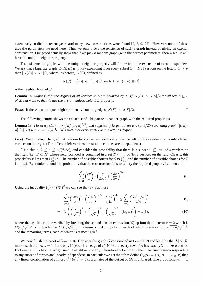
extensively studied in recent years and many new constructions were found [2, 7, 9, 22]. However, none of thesegive the parameters we need here. Thus we only prove the existence of such a graph instead of giving an explicitconstruction. Our proof actually show that if we pick a random graph (with the correct parameters) then w.h.p. it willhave the unique-neighbor property.
The existence of graphs with the unique neighbor property will follow from the existence of certain expanders.We say that a bipartite graph(L, R, E) is (σ, α)-expanding if for every subsetS ⊆ L of vertices on the left, if|S| ≤ σthen|N(S)| > α · |S|, where (as before)N(S), defined as
N(S) = v ∈ R : ∃u ∈ S such that (u, v) ∈ E,
is the neighborhood ofS.
Lemma 18. Suppose that the degrees of all vertices inL are bounded by∆. If |N(S)| > ∆|S|/2 for all setsS ⊆ Lof size at mostσ, thenG has theσ-right unique neighbor property.
Proof. If there is no unique neighbor, then by counting edges|N(S)| ≤ ∆|S|/2.
The following lemma shows the existence of a bi-partite expander graph with the required properties.
Lemma 19. For everyc(n) = o(√
n/(log n)3/4) and sufficiently largen there is a(σ, 3/2)-expanding graph([c(n) ·n], [n], E) with σ = n/(4e4c2(n)) such that every vertex on the left has degree 3.
Proof. We construct the graph at random by connecting each vertex onthe left to three distinct randomly chosenvertices on the right. (For different left vertices the random choices are independent.)
Fix a sizes, 2 ≤ s ≤ n/(2e2c), and consider the probability that there is a subsetS ⊆ [cn] of s vertices onthe right (i.e.S ⊂ R) whose neighborhood is contained in a setT ⊆ [n] of 3s/2 vertices on the left. Clearly, thisprobability is less than( 3s
2n)3s. The number of possible choices forS is(
cns
)
and the number of possible choices forTis(
n3s/2
)
. By a union bound, the probability that the construction fails to satisfy the required property is at most
σ∑
s=2
(
cn
s
)
·(
n
3s/2
)(
3s
2n
)3s
. (8)
Using the inequality(nk
)
≤(
nek
)kwe can see that(8) is at most
σ∑
s=2
(ecn
s
)s·(
2en
3s
)3s/2
·(
3s
2n
)3s
≤σ∑
s=2
(
2e3c√
s√n
)s
(9)
= O
(
(
c√n
)2
+
(
c√n
)3
+
(
c√n
)4
· (log n)3
)
= o(1), (10)
where the last line can be verified by breaking the second sum in expression (9) up into the the terms = 2 which isO((c/
√n)2; s = 3, which isO((c/
√n)3); the termss = 4, . . . , 2 log n, each of which is at mostO(c
√log n/
√n)4;
and the remaining terms, each of which is at most1/n2.
We now finish the proof of lemma 16. Consider the graphG constructed in Lemma 19 and letA be the|L| × |R|matrix such thatAv,u = 1 if and only if (v, u) is an edge ofG. Note that every row ofA has exactly 3 non-zero entries.By Lemma 18,G has theσ-right unique neighbor property. Therefore by Lemma 17 the linear functions correspondingto any subset ofσ rows are linearly independent. In particular we get that if we defineG2(x) = (A1 ·x, ..., Am ·x) thenany linear combination of at mostn2/4e2c2 − 1 coordinates of the output ofG2 is unbiased. The proof follows.
14

5.4 Putting Everything Together: Proof of theorem 4
In order to obtain the generator, recall thatm = cn and takeG1 : 0, 1n → 0, 1m, andG2 : 0, 1n → 0, 1m
be the generators defined above (with the parameterc). Then we takeG : 0, 12n → 0, 1m defined byG(x, y) =G1(x) ⊕ G2(y). We get that by lemma 12 any combination of more thanσ outputs ofG has bias at most2−σ/(c2+c),and that by lemma 16, any combination of at mostσ = n/(4e2c2) of the outputs ofG is unbiased. This completes theproof of the theorem.
5.5 Generator for k = 4
Whenk = 4 we want to replace the generator for small sets by a generatorwhich depends only on two bits. Theconstruction is essentially the one in [8].
Let H be an undirected graph withn vertices, that we identify with[n], havingcn edges and girthγ. Fix someordering of the edges ofH, and let(aj , bj) be thej-th edge ofH. We define the linear functionsl1, . . . , lm aslj(x1, . . . , xn) = xaj
+ xbj.
Proposition 20. For every subsetS ⊆ [m], |S| < γ, the functionlS(x) =∑
j∈S lj(x) is balanced.
Proof. Since|S| < γ, the subgraph ofH induced by the edges ofS is a forest. ThereforelS(x) is a non-zero linearfunction, and hence balanced.
The explicit construction of expanders by Lubotzky-Phillips-Sarnak [21] has high girth:
Lemma 21 ([21]). For everyc and for sufficiently largen there are explicitly constructible graphsH with n vertices,cn edges, and girthΩ((log n)/(log c)).
We thus obtain.
Theorem 22. For everyc and sufficiently largen, there is a generator in uniformNC04 mappingn bits intocn bits
and sampling anε-biased distribution, whereε = n−1/O(c2 log c).
6 ε-biased generator for largek
In this section we construct anε-biased generator inNC0k, for largek, that outputsnΩ(
√k) bits. More precisely we
prove Theorem 5:
Theorem. Letk be a positive integer. There exists anε-biased generator inNC0k fromn bits to
(
n√k − 6
)
√k
2−3
= n√
k( 12−ok(1))
bits whose biasε is at most
exp
(
− n1
2√
k
4 × 2√
k
)
.
6.1 The Generator for Large Tests
In this section we prove the following Lemma.
15

Lemma 23. Letn = p2 and letd be an integer. Then there exists a generatorG1 : (g1, . . . , gm) : 0, 1n → 0, 1m,wherem =
(
pd
)
such that for allJ ⊆ [m] the bias ofg =⊕
j∈J gj is at most
exp
(
−|J | 1d2d
)
. (11)
Proof. Consider the following bi-partite graphG = (L, R, E) where|L| = p (left vertices),|R| =(pd
)
(right vertices).
Identify the vertices ofL with the numbers1, ..., p and the vertices ofR with([p]
d
)
, the set of all subsets of[p]∆=
1, . . . , p of sized. The edges ofG are all pairs(i, S) such thati ∈ [p], S ∈([p]
d
)
andi ∈ S. For a set of vertices,V ,we denote withN(V ) the set of neighbors ofV :
N(V ) = u ∈ L ∪ R : ∃v ∈ V such that (u, v) ∈ E.
For a vertexi let deg(i) = |N(i)|.
Proposition 24. For any set of right verticesV ⊆ R we have that|N(V )| ≥ d|V |1d
e .
Proof. Note that for any set oft left vertices,L′, there are (exactly)(
td
)
right vertices,R′, such thatN(R′) = L′. Theresult follows from the inequality
|V | ≤(|N(V )|
d
)
≤(
e|N(V )|d
)d
.
Our construction will assign a monomial of degreed, in the input variables, to each edge. We think about thevertices ofL as representing disjoint subsets of the input variables (each of sizep) and each edge leaving such inputset as corresponding to a monomial in its variables. The right vertices,R, correspond to the output bits. Each outputis the sum of the monomials that label the edges that fan into it. We now give the formal construction.
Let X =⊔p
i=1 Xi be a partition ofX = x1, ..., xn into p disjoint sets each of sizep. We assign the setXi tothei-th vertex ofL. Let Mi be the set of all multilinear monomials of degreed in the variables ofXi. We have that
|Mi| =
(
p
d
)
>
(
p − 1
d − 1
)
= deg(i)
Therefore we can assign to each edge leavingi a different monomial fromMi. Denote byMe the monomial corre-sponding to the edgee. Each right vertex corresponds to an output bit. For a right vertexj thej’th output, which wedenote bygj , is the sum of all monomials that were assigned to the edges adjacent toj:
gj =∑
e:j∈e
Me.
Thus each output is the sum ofd monomials each of degreed. Hence each output depends ond2 input variables. Wenow show that any large linear combination of the output bitshas a small bias by proving (11). Letg =
⊕
j∈J gj. Theproof is essentially the same as the proof of lemma 12 and follows from the following easy propositions.
Proposition 25. Let g =⊕
j∈J gj , theng can be written as the sum of at leastN(J) polynomials of degreed, eachin a different set of variables.
Proof. The set of outputsJ , hasN(J) left neighbors. The edges connecting the setJ to a neighbori ∈ N(J) arelabeled with polynomials of degreed in Xi.
16

From the Schwartz-Zippel lemma [29, 32] we get
Proposition 26. For any polynomialg of degreed we have
1
2d≤ Pr[g = 0] ≤ 1 − 1
2d.
Thus according to lemma 14 we get that the bias ofg is at most
1
2
(
1 − 2
2d
)N(J)
≤ 1
2· exp
(−2N(J)
2d
)
≤ exp
(
−|J |1d
2d
)
This finishes the proof of Lemma 23.
6.2 The Generator for Small Tests
Similar to thek = 4, 5 cases this generator will output only linear functions. We will have the property that any smallset of these linear functions is linearly independent. Thisis a standard construction that follows from unique neighborproperty of expanding graphs.
Lemma 27. Let t be positive integert and∆ = 10t. There exists a mapping fromn bits tont bits such that everyoutput depends linearly on∆ input variables, and such that any linear combination of at most
√n outputs is non-zero
and therefore unbiased.
Proof. As in the proof of lemma 16, we shall construct a linear mapping from an expander bi-partite graph with theunique neighbor property. We first prove:
Lemma 28. Let t be a positive integer and∆ = 10t. Then there exists a family of bi-partite graphsGn = (L, R, E)with |L| = nt, |R| = n, ∀v ∈ L deg(v) = ∆, such thatGn is a (σ = ⌈√n⌉, 5t) expanding graph.
Proof. Let |R| = n, |L| = nt. Connect every vertex inL to a randomly chosen multi set of size∆ of distinct rightvertices. We continue as in Lemma 19. Fix a sizes, 2 ≤ s ≤ σ = ⌈√n⌉, and consider the probability that thereis a subsetS ⊆ [nt] of s vertices on the right whose neighborhood is contained in a set T ⊆ [n] of ∆s/2 verticeson the left. This probability is less than(∆s
2n )∆s. The number of possible choices forS is(
nt
s
)
and the number ofpossible choices forT is
(
n∆s/2
)
. Therefore applying the union bound and recalling that∆ = 10t the probability thatthe construction fails to satisfy the required property is at most
σ∑
s=2
(
ent
s
)s
·(
2en
∆s
)∆s/2
·(
∆s
2n
)∆s
≤σ∑
s=2
(
(e∆s)∆
n4t
)s
= o(1).
We now finish the proof of lemma 27. LetG be the graph constructed in Lemma 28. Label each vertex on theright by one of the variablesxi and each vertex on the left by the linear combination of the variables adjacent to it. ByLemma 18,G has theσ-right unique neighbor property. Therefore by Lemma 17 every set consisting ofσ − 1 linearfunctions (corresponding to left vertices) is linearly independent. The proof follows.
17

6.3 Putting things together: Proof of theorem 5
Let κ = (⌊√
k⌋ − 5)2, ν = ⌊√
n2 ⌋
2. We have that
k > κ + 10√
κ, κ > k − 12√
k, n2 ≥ ν > n
2 −√
2n.
Let X = x1, ..., xν, Y = y1, ..., yν. Let f1(X), . . . , f(pd)
(X) be the outputs of the generator against large tests
with the parametersp =√
ν, d =√
κ. Let h1(Y ), . . . , hνκ(Y ) be the outputs of the generator for small tests onY ,given the parametert =
√κ. Note that
νκ >
(√ν√κ
)
=
(
p
d
)
.
Our generatorG will output the functions
∀1 ≤ i ≤(
p
d
)
gi(X, Y ) = fi(X) + hi(Y ).
Notice that as we have morehi’s thanfi’s we do not use most of thehi’s. Clearly, each output of the generator dependson κ + 10
√κ < k input variables. From lemmas 23,27 we get that the bias of anynon trivial linear combination of
the outputs is at most
exp
(
−ν1d
2d
)
≤ exp
(
− n1
2√
k
4 × 2√
k
)
.
Our generator takes2ν ≤ n inputs and outputs
(
p
d
)
≥(
e2ν
κ
)
√κ
2
≥(
n√k − 6
)
√k
2−3
= n√
k( 12−ok(1))
as needed.
7 A degree2 generator
In this section we consider a variant of the problem presented in the paper. Suppose that we require that every output bitis a degreek polynomial in the input bits. It is clear that if we want the output to beε-biased, then the number of outputbits m is at most the dimension of the space of degreek polynomials inn variables, which is
∑ki=0
(ni
)
= O(nk)(as otherwise there will be a linear dependence among the output bits). Clearly this is a relaxation of the problemdescribed above. In particular any upper bound here will imply an upper bound forNC0
k. The problem is also ofindependent interest, as low degree generators are “simple” in an intuitive sense.
We now show how to construct a generator ofε-biased set such that every output is a polynomial of degree2 inthe input variables. We show that unlike the NC2
0 case we can outputΩ(n2) bits. In particular we prove Theorem 6:
Theorem. ∀1 ≤ m ≤ n there exists anε-biased generatorG = (g1, ..., gt) : 0, 1n 7→ 0, 1t, t = ⌊n2 ⌋ · m, such
thatgi is a degree2 polynomial, and the bias of any non trivial linear combination of thegi’s is at most2−n−2m
4 .
We begin by studying the bias of a degree2 polynomial, overGF (2). In this section we will only consider degree2 polynomialsP such thatP (0) = 0. Below we denote withxT andAT the transpose of the vectorx and the matrixA, respectively.
18
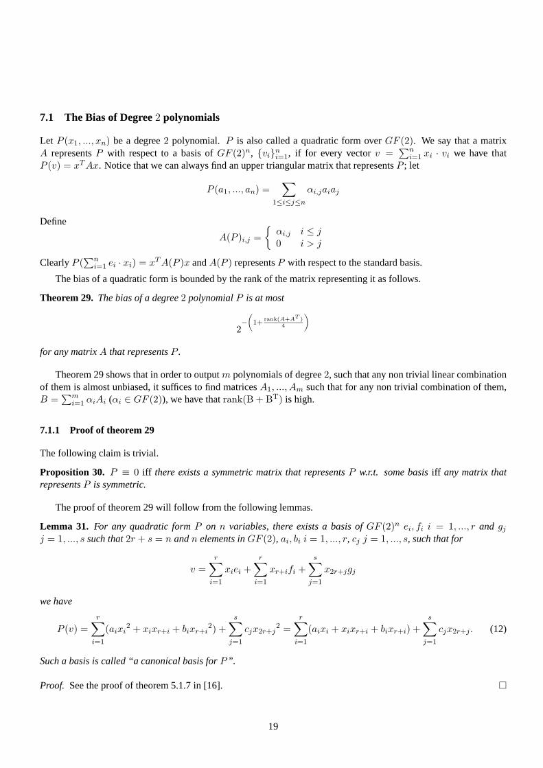
7.1 The Bias of Degree2 polynomials
Let P (x1, ..., xn) be a degree2 polynomial. P is also called a quadratic form overGF (2). We say that a matrixA representsP with respect to a basis ofGF (2)n, vin
i=1, if for every vectorv =∑n
i=1 xi · vi we have thatP (v) = xT Ax. Notice that we can always find an upper triangular matrix that representsP ; let
P (a1, ..., an) =∑
1≤i≤j≤n
αi,jaiaj
Define
A(P )i,j =
αi,j i ≤ j0 i > j
ClearlyP (∑n
i=1 ei · xi) = xT A(P )x andA(P ) representsP with respect to the standard basis.
The bias of a quadratic form is bounded by the rank of the matrix representing it as follows.
Theorem 29. The bias of a degree2 polynomialP is at most
2−(
1+rank(A+AT )
4
)
for any matrixA that representsP .
Theorem 29 shows that in order to outputm polynomials of degree2, such that any non trivial linear combinationof them is almost unbiased, it suffices to find matricesA1, ..., Am such that for any non trivial combination of them,B =
∑mi=1 αiAi (αi ∈ GF (2)), we have thatrank(B + BT) is high.
7.1.1 Proof of theorem 29
The following claim is trivial.
Proposition 30. P ≡ 0 iff there exists a symmetric matrix that representsP w.r.t. some basisiff any matrix thatrepresentsP is symmetric.
The proof of theorem 29 will follow from the following lemmas.
Lemma 31. For any quadratic formP on n variables, there exists a basis ofGF (2)n ei, fi i = 1, ..., r and gj
j = 1, ..., s such that2r + s = n andn elements inGF (2), ai, bi i = 1, ..., r, cj j = 1, ..., s, such that for
v =
r∑
i=1
xiei +
r∑
i=1
xr+ifi +
s∑
j=1
x2r+jgj
we have
P (v) =
r∑
i=1
(aixi2 + xixr+i + bixr+i
2) +
s∑
j=1
cjx2r+j2 =
r∑
i=1
(aixi + xixr+i + bixr+i) +
s∑
j=1
cjx2r+j. (12)
Such a basis is called “a canonical basis forP ”.
Proof. See the proof of theorem 5.1.7 in [16].
19

Lemma 32. Let P be a quadratic form onn variables LetA representP with respect to the standard basis (inparticular,A is upper triangular) andD representP with respect to the canonical basis. Then
rank(D) ≥ rank(A + AT )
2
Proof. Let B be the matrix whose columns aree1, ..., er, f1, ..., fr, g1, ..., gs written w.r.t. the standard basis. We havethat
∀x ∈ GF (2)n xT Dx = xT BT ABx.
In other words∀x ∈ GF (2)n xT (D − BT AB)x = 0.
Therefore there exists a symmetric matrixS such that
D − BT AB = S,
orD = BT (A + (B−1)T S(B−1))B.
As (B−1)T S(B−1) is a symmetric matrix we get by the next lemma (lemma 33) that
rank(D) = rank(A + (B−1)T S(B−1)) ≥ rank(A + AT )
2.
Lemma 33. For an upper triangular matrixA and any symmetric matrixS we have that
rank(A + S) ≥ rank(A + AT )
2.
Proof. Let r = rank(A + S) = rank(
(A + S)T)
= rank(AT + S). Then
rank(A + AT ) = rank(A + S + S + AT ) ≤ rank(A + S) + rank(AT + S) = 2r.
PROOF OF THEOREM29. Clearly the bias ofP does not change if we calculate it w.r.t. to a canonical basis, vini=1.
Let v =∑n
i=1 xi · vi, we have that
P (v) =r∑
i=1
(aixi + xixr+i + bixr+i) +s∑
j=1
cjx2r+j.
Note that if for some1 ≤ j ≤ s cj 6= 0 thenP is unbiased. Otherwise, we get by proposition 26 that for every i thebias of(aixi
2 +xixr+i + bixr+i2) is at most14 . Therefore according to Lemma 14 we get that the bias ofP is at most
(
12
)r+1. As we assumed that∀j cj = 0 we see that
r ≥ rank(D)
2.
The theorem now follows from lemma 32.
20

7.2 The generator
In this subsection we give a construction of a linear space ofmatrices with the property that for every non zero matrixin the space,A, we have thatrank(A + AT ) is high. Such a construction was first given by Roth [28], and latersimplified by Meshulam [24] (see also [30]). For completeness we give the construction here.
Theorem 34. For any positive natural numbersn ≥ m there existt = ⌊n2 ⌋ · m matricesA1, ..., At ∈ Mn(GF (2))
such that for every non trivial combinationB =∑t
i=1 αiAi we have that
rank(B + BT ) ≥ n − 2m
Proof. Denote withF = GF (2n) the field with2n elements.F is a linear space overGF (2) of dimensionn. We willabuse notation and think about eachy ∈ F both as a field element and as a vector inGF (2)n. Fix a basis forF overGF (2) of the form1, x, x2, ..., xn−1 for somex ∈ F. Each element,y ∈ F, can be viewed as a linear transformationof F overGF (2) in the following manner:
∀z ∈ F y(z) = y · z .
Thus for everyy ∈ F there is a corresponding matrixAy ∈ Mn(GF (2)), that representsy over the basis we chose.We denoteA = Ax (the samex as in the basis).
Let ϕ : F 7→ F be the Frobenius transformation, that isϕ(y) = y2. Let ϕ(k) = ϕ ϕ... ϕ, k times. That isϕ(k)(y) = y2k
. It is easy to see thatϕ is a linear transformation ofF overGF (2). We denote withB the matrix thatrepresentsϕ over our basis. That is, by abusing notations,
∀y ∈ F By = y2
Let V ⊆ Mn(GF (2)) be the linear space spanned by the matrices
V = span Ai · Bj | i = 0, ..., n − 1 , j = 0, ..., m − 1
Lemma 35. V is a linear space of matrices of dimensionnm such that for any0 6= E ∈ V we have that
rank(E) > n − m
Proof. Let 0 6= E ∈ V . We want to calculatedim(ker(E)). For anyy ∈ F we think aboutEy also as an element ofGF (2)n. It is clear that
Ey =
n−1∑
i=0
m−1∑
j=0
αi,jAi · Bj
y
=n−1∑
i=0
m−1∑
j=0
αi,jAi(y2j
) =n−1∑
i=0
m−1∑
j=0
αi,jxiy2j
.
That is,Ey is a polynomial of degree2m−1 in y. Therefore it has at most2m−1 roots. AsE is a linear transformation,we get that its roots are a linear space. Since there are at most 2m−1 roots, the dimension ofker(E) is at mostm− 1.Hencerank(E) ≥ n − m + 1.
We now finish the proof of the theorem. LetV be the space guaranteed by lemma 35 inM⌊n2⌋(GF (2)) of
dimensiont = ⌊n2 ⌋ · m. Let E1, ..., Et be a basis forV . Let Ai be an × n matrix of the following form
Ai =
(
0 Ei
0 0
)
21

Where the0 stands for the all zero matrix inM⌊n2⌋(GF (2)). For any non trivial combinationB =
∑ti=1 αiAi we get
B =t∑
i=1
αiAi =
(
0∑t
i=1 αiEi
0 0
)
=
(
0 E0 0
)
whereE =∑t
i=1 αiEi. SinceEi is a basis and not all theαi’s are zero then0 6= E ∈ V . Thereforerank(E) ≥⌊n
2 ⌋ − m + 1. We get that
rank(B + Bt)
= rank
(
0 EE 0
)
= 2 · rank(E)
≥ 2(
⌊n
2⌋ − m + 1
)
≥ n − 2m
Proof of Theorem 6: Let A1, ..., At be the matrices guaranteed by theorem 34. Definegi(x) = xT Aix. Consider anynon trivial linear combination
g(x) =t∑
i=1
αigi(x) = xT
(
n∑
i=1
αiAi
)
x.
According to theorem 34, we have thatrank(g) ≥ n − 2m. Theorem 29 shows that the bias ofg is at most2n−2m
4 .
Acknowledgements
We wish to thank David Wagner for suggesting the relevance ofcorrelation attacks. A.S. would also like to thank AviWigderson for helpful discussions. The authors would like to thank the anonymous referees for numerous valuablecomments that greatly improved the presentation of the paper.
22

References
[1] B. Applebaum, Y. Ishai, and E. Kushilevitz. Cryptography in NC0. In Proceedings of the 45th IEEE Symposiumon Foundations of Computer Science, pages 166-175, 2004.
[2] N. Alon, M. Capalbo. Explicit Unique-Neighbor Expanders. In Proceedings of the 43rd IEEE Symposium onFoundations of Computer Science, pages 73-79, 2000.
[3] N. Alon, O. Goldreich, J. Hastad, and R. Peralta. Simple constructions of almostk-wise independent randomvariables.Random Structures and Algorithms, 3(3):289–304, 1992.
[4] P. Beame, R. Karp, T. Pitassi, and M. Saks. On the complexity of unsatisfiability proofs for random k-cnfformulas. InProceedings of the 30th ACM Symposium on Theory of Computing, pages 561-571, 1998.
[5] A. Bogdanov, K. Obata, and L. Trevisan. A lower bound for testing 3-colorability in bounded degree graphs. InProceedings of the 43rd IEEE Symposium on Foundations of Computer Science, pages 93–102, 2002.
[6] E. Ben-Sasson and A. Wigderson. Short proofs are narrow:Resolution made simple.Journal of the ACM, 48(2),2001.
[7] M. Capalbo. Explicit Constant-Degree Unique-NeighborExpanders, 2001.
[8] M. Cryan and P. B. Miltersen. On pseudorandom generatorsin NC0. In Proceedings of 26th MathematicalFoundations of Computer Science, pages 272-284, 2001.
[9] M. Capalbo, O. Reingold, S. Vadhan and A. Wigderson. Randomness Conductors and Constant-Degree Expan-sion Beyond the Degree/2 Barrier. InProceedings of the 34th ACM Symposium on the Theory of Computing,659-668, 2000.
[10] Oded Goldreich. Three XOR-Lemmas - An Exposition. Electronic Colloquium on Computational Complexity(ECCC) 2(56): (1995)
[11] O. Goldreich, S. Goldwasser, and S. Micali. How to construct random functions.Journal of the ACM, 33(4):792–807, 1986.
[12] O. Goldreich. Candidate one-way functions based on expander graphs. Electronic Colloquium on ComputationalComplexity (ECCC) TR00-090, 2000.
[13] M.X. Goemans and D.P. Williamson. Improved approximation algorithms for maximum cut and satisfiabilityproblems using semidefinite programming.Journal of the ACM, 42(6):1115–1145, 1995.
[14] J. Hastad. Some optimal inapproximability results. InProceedings of the 29th ACM Symposium on Theory ofComputing, pages 1-10, 1997.
[15] J. Hastad, R. Impagliazzo, L. Levin, and M. Luby. A pseudorandomgenerator from any one-way function.SIAMJournal on Computing, 28(4):1364–1396, 1999.
[16] J. W. P. Hirschfeld, Projective Geometries over FiniteFields, Oxford University Press, 1979.
[17] R. Impagliazzo and M. Naor. Efficient cryptographic schemes provably as secure as subset sum.Journal ofCryptology, 9(4):199–216, 1996.
23

[18] T. Johansson and F. Jonsson. Improved fast correlation attacks on stream ciphers via convolutional codes. InProceedings of International Conference on the Theory and Application of Cryptographic Techniques (EURO-CRYPT), pages 347-362, 1999.
[19] M. Kharitonov. Cryptographic hardness of distribution-specific learning. InProceedings of 25th ACM Sympo-sium on Theory of Computing, pages 372-381, 1993.
[20] N. Linial, Y. Mansour, and N. Nisan. Constant depth circuits, fourier transform and learnability.Journal of theACM, 40(3):607–620, 1993.
[21] A. Lubotzky, R. Phillips, and P. Sarnak. Ramanujan graphs. Combinatorica, 8:261–277, 1988.
[22] C. J. Lu and O. Reingold and S. Vadhan and A. Wigderson Extractors: Optimal Up to Constant Factors. Inproceedings of the 35th ACM Symposium on the Theory of Computing, pages 602-611, 2003.
[23] M. Luby and C. Rackoff. How to construct pseudorandom permutations from pseudorandom functions.SIAMJournal on Computing, 2(17):373–386, 1988.
[24] R. Meshulam. Spaces of Hankel matrices over finite fields, Linear Algebra and its Applications218:73-76,1995.
[25] E. Mossel, R. O’Donnell and R. Servedio. Learning Juntas. Inproceedings of the 35th ACM Symposium on theTheory of Computing, pages 206–212, 2003.
[26] E. Mossel, A. Shpilka and L. Trevisan. Onε-biased generators inNC0. In Proceeding of the 44th IEEESymposium on Foundations of Computer Science, pages 136–145, 2003.
[27] J. Naor and M. Naor. Small-bias probability spaces: efficient constructions and applications,SIAM Journal onComputing, 22(4):838–856, 1993.
[28] R. Roth. Maximum rank array codes and their applicationto crisscross error correction,IEEE Transactions onInformation Theory37:328–336, 1991.
[29] J. T. Schwartz. Fast probabilistic algorithms for verification of polynomial identities.Journal of the ACM,27(4):701–717, 1980.
[30] A. Shpilka. On the rigidity of matrices. Manuscript, 2002.
[31] U. Vazirani.Randomness, Adversaries and Computation. PhD thesis, University of California, Berkeley, 1986.
[32] R. Zippel. Probabilistic algorithms for sparse polynomials. InSymbolic and algebraic computation (EUROSAM),pages 216–226, 1979.
24