on a q-central limit theorem consistent with nonextensive - cbpf
TRANSCRIPT

Milan j. math. 76 (2008), 307–328
c© 2008 Birkhauser Verlag Basel/Switzerland
1424-9286/010307-22, published online 14.3.2008
DOI 10.1007/s00032-008-0087-y Milan Journal of Mathematics
On a q-Central Limit TheoremConsistent with NonextensiveStatistical Mechanics
Sabir Umarov, Constantino Tsallis and Stanly Steinberg
Abstract. The standard central limit theorem plays a fundamental rolein Boltzmann-Gibbs statistical mechanics. This important physical the-ory has been generalized [1] in 1988 by using the entropy Sq = 1−∑ i pq
i
q−1
(with q ∈ R) instead of its particular BG case S1 = SBG = −∑i pi ln pi.The theory which emerges is usually referred to as nonextensive statis-tical mechanics and recovers the standard theory for q = 1. During thelast two decades, this q-generalized statistical mechanics has been suc-cessfully applied to a considerable amount of physically interesting com-plex phenomena. A conjecture[2] and numerical indications available inthe literature have been, for a few years, suggesting the possibility ofq-versions of the standard central limit theorem by allowing the ran-dom variables that are being summed to be strongly correlated in somespecial manner, the case q = 1 corresponding to standard probabilisticindependence. This is what we prove in the present paper for 1 ≤ q < 3.The attractor, in the usual sense of a central limit theorem, is given bya distribution of the form p(x) = Cq[1− (1 − q)βx2]1/(1−q) with β > 0,and normalizing constant Cq. These distributions, sometimes referredto as q-Gaussians, are known to make, under appropriate constraints,extremal the functional Sq (in its continuous version). Their q = 1 andq = 2 particular cases recover respectively Gaussian and Cauchy distri-butions.
Mathematics Subject Classification (2000). Primary 60F05; Secondary60E07, 60E10, 82Cxx.
Keywords. q-central limit theorem, correlated random variables, nonex-tensive statistical mechanics.

308 Umarov, Tsallis and Steinberg Vol. 76 (2008)
1. Introduction
Limit theorems and, particularly, the central limit theorems (CLT), surelyare among the most important theorems in probability theory and statis-tics. They play an essential role in various applied sciences, including sta-tistical mechanics. Historically A. de Moivre, P.S. de Laplace, S.D. Poissonand C.F. Gauss have first shown that Gaussian is the attractor of indepen-dent systems with a finite second variance. Chebyshev, Markov, Liapounov,Feller, Lindeberg, Levy have contributed essentially to the development ofthe central limit theorem.
It is well known in the classical Boltzmann-Gibbs (BG) statistical me-chanics that the Gaussian maximizes, under appropriate constraints, theBoltzmann-Gibbs entropy SBG = −∑i pi ln pi (SBG = − ∫ dx p(x) ln p(x)in its continuous form). The q-generalization of the classic entropy intro-duced in [1] as the basis for generalizing the BG theory, and given bySq = 1−∑i pq
iq−1 (Sq =
[1− ∫ dx [p(x)]q
]/(q − 1) in its continuous form), with
q ∈ R and S1 = SBG, reaches its maximum at the distributions usually re-ferred to as q-Gaussians (see [3]). This fact, and a number of conjectures [2],numerical indications [4], and the content of some other studies [1, 3, 5, 6]suggest the existence of a q-analog of the CLT as well. In this paper weprove a generalization of the CLT for 1 ≤ q < 3. The case q < 1 requiresessentially different technique, therefore we leave it for a separate paper.
In the classical CLT, the random variables are required to be indepen-dent. Central limit theorems were established for weakly dependent randomvariables also. An introduction to this area can be found in [7, 8, 9, 10, 11,12] (see also references therein), where different types of dependence areconsidered, as well as the history of the developments. The CLT does nothold if correlation between far-ranging random variables is not neglectable(see [13]). Nonextensive statistical mechanics deals with strongly correlatedrandom variables, whose correlation does not rapidly decrease with increas-ing ’distance’ between random variables localized or moving in some geo-metrical lattice (or continuous space) on which a ’distance’ can be defined.This type of correlation is sometimes referred to as global correlation (see[17] for more details).
In general, q-CLT appears to be untractable if we rely on the clas-sic algebra. However, nonextensive statistical mechanics uses constructionsbased on a special algebra sometimes referred to as q-algebra, which de-pends on parameter q. We show that, in the framework of q-algebra, the
Vol. 76 (2008) q-CLT Consistent with Nonextensive Statistical Mechanics 309
corresponding q-generalization of the central limit theorem becomes possi-ble and relatively simple.
The theorems obtained in this paper are represented as a series oftheorems depending on the type of correlations. We will consider three typesof correlation. An important distinction from the classic CLT is the fact thata complete formulation of q-CLT is not possible within only one given q.The parameter q is connected with two other numbers, q∗ = z−1(q) and q∗ =z(q), where z(s) = (1+s)/(3−s). We will see that q∗ identifies an attractor,while q∗ yields the scaling rate. In general, the present q-generalization ofthe CLT is connected with a triplet (qk−1, qk, qk+1) determined by a givenq ∈ [1, 2). For systems having correlation identified by qk, the index qk−1
determines the attracting q-Gaussian, while the index qk+1 indicates thescaling rate. Note that, if q = 1, then the entire family of theorems reducesto one element, thus recovering the classic CLT.
The paper is organized as follows. In Section 2 we recall the basics ofq-algebra, definitions of q-exponential and q-logarithm. Then we introducea transform Fq and study its basic properties. For q = 1 Fq is not a linearoperator. Note that Fq is linear only if q = 1 and in this case coincideswith the classic Fourier transform. Lemma 2.5 implies that Fq is invertiblein the class of q-Gaussians. An important property of Fq is that it mapsa q-Gaussian to a q∗-Gaussian (with a constant factor). In Section 3 weprove the main result of this paper, i.e., the q-version of the CLT. We in-troduce the notion of q-independent random variables (three types), whichclassify correlated random variables. Only in the case q = 1 the correlationdisappears, thus recovering the classic notion of independence of randomvariables.
2. q-Algebra and q-Fourier Transform
2.1. q-sum and q-product
The basic operations of the q-algebra appear naturally in nonextensivestatistical mechanics. It is well known that, if A and B are two independentsubsystems, then the total BG entropy satisfies the additivity property
SBG(A + B) = SBG(A) + SBG(B).
Additivity is not preserved for q = 1. Indeed, we easily verify [1, 3, 2]
Sq(A + B) = Sq(A) + Sq(B) + (1− q)Sq(A)Sq(B).
310 Umarov, Tsallis and Steinberg Vol. 76 (2008)
Introduce the q-sum of two numbers x and y by the formula
x⊕q y = x + y + (1− q)xy.
Then, obviously, Sq(A + B) = Sq(A) ⊕q Sq(B). It is readily seen that theq-sum is commutative, associative, recovers the usual summing operationif q = 1 (i.e. x ⊕1 y = x + y), and preserves 0 as the neutral element (i.e.x ⊕q 0 = x). By inversion, we can define the q-subtraction as x q y =
x−y1+(1−q)y . Further, the q-product for x, y is defined by the binary relation
x⊗qy = [x1−q+y1−q−1]1
1−q
+ . The symbol [x]+ means that [x]+ = x, if x ≥ 0,and [x]+ = 0, if x ≤ 0. Also this operation is commutative, associative,recovers the usual product when q = 1 (i.e. x ⊗1 y = xy), preserves 1 asthe unity (i.e. x⊗q 1 = x). Again, by inversion, a q-division can be defined:
xqy = [x1−q−y1−q+1]1
1−q
+ . Note that, for q = 1, division by zero is allowed.As we will see below, the q-sum and the q-product are connected eachother through the q-exponential, generalizing the fundamental property ofthe exponential function, ex+y = exey (or ln(xy) = ln x + ln y in terms oflogarithm).
2.2. q-exponential and q-logarithm
The q-analysis relies essentially on the analogs of exponential and logarith-mic functions, which are called q-exponential and q-logarithm [18]. In themathematical literature there are other generalizations of the classic expo-nential distinct from the q-exponential used in the present paper. Thesegeneralizations were introduced by Euler [14], Jackson [15], and others. See[16] for details.
The q-exponential and q-logarithm, which are denoted by exq and lnq x,
are respectively defined as exq = [1+(1−q)x]
11−q
+ and lnq x = x1−q−11−q , (x > 0).
For the q-exponential, the relations ex⊕qyq = ex
qeyq and ex+y
q = exq ⊗q ey
q
hold true. These relations can be rewritten equivalently as follows:lnq(x⊗q y) = lnq x + lnq y, and lnq(xy) = lnq x⊕q lnq y1. The q-exponentialand q-logarithm have asymptotics ex
q = 1 + x + q2x2 + o(x2), x → 0 and
lnq(1+x) = x− q2x2 + o(x2), x→ 0. For q = 1, we can define eiy
q , where i is
the imaginary unit and y is real, as the principal value of [1+ i(1− q)y]1
1−q ,
1These properties reflect the possible extensivity of the nonadditive entropy Sq in the
presence of special correlations [17, 24, 26, 28, 29].
Vol. 76 (2008) q-CLT Consistent with Nonextensive Statistical Mechanics 311
namely
eiyq = [1 + (1− q)2y2]
12(1−q) e
i arctan[(q−1)y]q−1 , q = 1.
Analogously, for z = x + iy we can define ezq = ex+iy
q , which is equal toexq ⊗q eiy
q in accordance with the property mentioned above. Note that, if
q < 1, then for real y, |eiyq | ≥ 1 and |eiy
q | ∼ (1+y2)1
2(1−q) , x→∞. Similarly,if q > 1, then 0 < |eiy
q | ≤ 1 and |eiyq | → 0 if |y| → ∞.
2.3. q-Gaussian
Let β be a positive number. We call the function
Gq(β;x) =√
β
Cqe−βx2
q . (2.1)
a q-Gaussian; Cq is the normalizing constant, namely Cq =∫∞−∞ e−x2
q dx. Itis easy to verify that
Cq =
2√1−q
∫ π/20 (cos t)
3−q1−q dt =
2√
π Γ(
11−q
)
(3−q)√
1−q Γ(
3−q2(1−q)
) , −∞ < q < 1,√
π, q = 1,
2√q−1
∫∞0 (1 + y2)
−1q−1 dy =
√π Γ(
3−q2(q−1)
)
√q−1Γ
(1
q−1
) , 1 < q < 3 .
(2.2)For q < 1, the support of Gq(β;x) is compact since this density vanishes for|x| > 1/
√(1− q)β. Notice also that, for q < 5/3 (5/3 ≤ q < 3), the variance
is finite (diverges). Finally, we can easily check that there are relationships
between different values of q. For example, e−x2
q =[e−qx2
2− 1q
] 1q.
The following lemma establishes a general relationship (which containsthe previous one as a particular case) between different q-Gaussians.
Lemma 2.1. For any real q1, β1 > 0 and δ > 0 there exist uniquely deter-mined q2 = q2(q1, δ) and β2 = β2(δ, β1), such that
(e−β1x2
q1)δ = e−β2x2
q2.
Moreover, q2 = δ−1(δ − 1 + q1), β2 = δβ1.
Proof. Let q1 ∈ R1, β1 > 0 and δ > 0 be any fixed real numbers. For theequation
(1− (1− q1)β1x2)
δ1−q1 = (1− (1− q2)β2x
2)1
1−q2

312 Umarov, Tsallis and Steinberg Vol. 76 (2008)
to be an identity, it is needed (1 − q1)β1 = (1 − q2)β2, 1 − q1 = δ(1 − q2).These equations have a unique solution q2 = δ−1(δ− 1 + q1), β2 = δβ1.
The set of all q-Gaussians with a positive constant factor will be de-noted by Gq, i.e.,
Gq = bGq(β, x) : b > 0, β > 0.2.4. q-Fourier transform
From now on we assume that 1 ≤ q < 3. For these values of q we introducethe q-Fourier transform Fq, an operator which coincides with the Fouriertransform if q = 1. Note that the q-Fourier transform is defined on thebasis of the q-product and the q-exponential, and, in contrast to the usualFourier transform, is a nonlinear transform for q ∈ (1, 3). Let f be a non-negative measurable function with supp f ⊆ R. The q-Fourier transformfor f is defined by the formula
Fq[f ](ξ) =∫
supp feixξq ⊗q f(x)dx , (2.3)
where the integral is understood in the Lebesgue sense. For discrete func-tions fk, k ∈ Z = 0,±1, . . ., Fq is defined as
Fq[f ](ξ) =∑
k∈Zf
eikξq ⊗q fk , (2.4)
where Zf = k ∈ Z : fk = 0.In what follows we use the same notation in both cases. We also call
(2.3) or (2.4) the q-characteristic function of a given random variable Xwith an associated density f(x), using the notations Fq(X) or Fq(f) equiv-alently. The following lemma establishes the expression of the q-Fouriertransform in terms of the standard product, instead of the q-product.
Lemma 2.2. The q-Fourier transform can be written in the form
Fq[f ](ξ) =∫ ∞
−∞f(x) eixξ[f(x)]q−1
q dx. (2.5)
Proof. For x ∈ supp f we have
eixξq ⊗q f(x) = [1 + (1− q)ixξ + [f(x)]1−q − 1]
11−q =
f(x)[1 + (1− q)ixξ[f(x)]q−1]1
1−q . (2.6)
Integrating both sides of Eq. (2.6) we obtain (2.5).
Vol. 76 (2008) q-CLT Consistent with Nonextensive Statistical Mechanics 313
Analogously, for a discrete fk, k ∈ Z, (2.4) can be represented as
Fq[f ](ξ) =∑
k∈Zfke
ikξfq−1k
q .
Corollary 2.3. The q-Fourier transform exists for any nonnegative f ∈L1(R). Moreover, |Fq[f ](ξ)| ≤ ‖f‖L1 .
2
Proof. This is a simple implication of Lemma 2.2 and of the asymptoticsof eix
q for large |x| mentioned above.
Corollary 2.4. Assume f(x) ≥ 0, x ∈ R and Fq[f ](ξ) = 0 for all ξ ∈ R.Then f(x) = 0 for almost all x ∈ R.
Lemma 2.5. Let 1 ≤ q < 3. For the q-Fourier transform of a q-Gaussian,the following formula holds:
Fq[Gq(β;x)](ξ) =(e− ξ2
4β2−qC2(q−1)q
q
) 3−q2
. (2.7)
Proof. Denote a =√
βCq
and write
Fq[a e−βx2
q ](ξ) =∫ ∞
−∞(a e−βx2
q )⊗q (eixξq )dx
using the property ex+yq = ex
q ⊗q eyq of the q-exponential, in the form
Fq[ae−βx2
q ](ξ) = a
∫ ∞
−∞e−βx2+iaq−1xξq dxa
∫ ∞
−∞e−(
√βx− iaq−1ξ
2√
β)2− a2(q−1)ξ2
4βq dx
= a
∫ ∞
−∞e−(
√βx− iaq−1ξ
2√
β)2
q ⊗q e− a2(q−1)ξ2
4βq dx.
The substitution y =√
βx− iaq−1ξ2√
βyields the equation
Fq[ae−βx2
q ](ξ) =a√β
∫ ∞+iη
−∞+iηe−y2
q ⊗q e− a2(q−1)ξ2
4βq dy ,
where η = ξaq−1
2√
β. Moreover, the Cauchy theorem on integrals over closed
curves is applicable because of at least a power-law decay of q-exponential
2Here, and elsewhere, ‖f‖L1 =∫R f(x)dx, L1 being the space of absolutely integrable
functions.
314 Umarov, Tsallis and Steinberg Vol. 76 (2008)
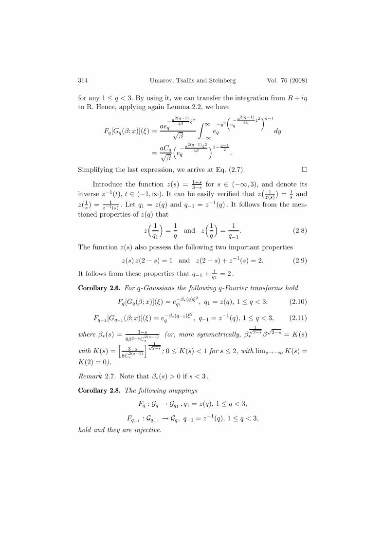
for any 1 ≤ q < 3. By using it, we can transfer the integration from R + iη
to R. Hence, applying again Lemma 2.2, we have
Fq[Gq(β;x)](ξ) =ae
− a2(q−1)
4βξ2
q √β
∫ ∞
−∞e−y2
(e−a2(q−1)
4βξ2
q
)q−1
q dy
=aCq√
β
(e− a2(q−1)ξ2
4βq
)1− q−12
.
Simplifying the last expression, we arrive at Eq. (2.7).
Introduce the function z(s) = 1+s3−s for s ∈ (−∞, 3), and denote its
inverse z−1(t), t ∈ (−1,∞). It can be easily verified that z(
1z(s)
)= 1
s andz(1
s ) = 1z−1(s)
. Let q1 = z(q) and q−1 = z−1(q) . It follows from the men-tioned properties of z(q) that
z( 1
q1
)=
1q
and z(1
q
)=
1q−1
. (2.8)
The function z(s) also possess the following two important properties
z(s) z(2 − s) = 1 and z(2− s) + z−1(s) = 2. (2.9)
It follows from these properties that q−1 + 1q1
= 2 .
Corollary 2.6. For q-Gaussians the following q-Fourier transforms hold
Fq[Gq(β;x)](ξ) = e−β∗(q)ξ2
q1, q1 = z(q), 1 ≤ q < 3; (2.10)
Fq−1 [Gq−1(β;x)](ξ) = e−β∗(q−1)ξ2
q , q−1 = z−1(q), 1 ≤ q < 3, (2.11)
where β∗(s) = 3−s
8β2−sC2(s−1)s
(or, more symmetrically, β1√2−s∗ β
√2−s = K(s)
with K(s) =[
3−s
8C2(s−1)s
] 1√2−s ; 0 ≤ K(s) < 1 for s ≤ 2, with lims→−∞ K(s) =
K(2) = 0).
Remark 2.7. Note that β∗(s) > 0 if s < 3 .
Corollary 2.8. The following mappings
Fq : Gq → Gq1 , q1 = z(q), 1 ≤ q < 3,
Fq−1 : Gq−1 → Gq, q−1 = z−1(q), 1 ≤ q < 3,
hold and they are injective.
Vol. 76 (2008) q-CLT Consistent with Nonextensive Statistical Mechanics 315
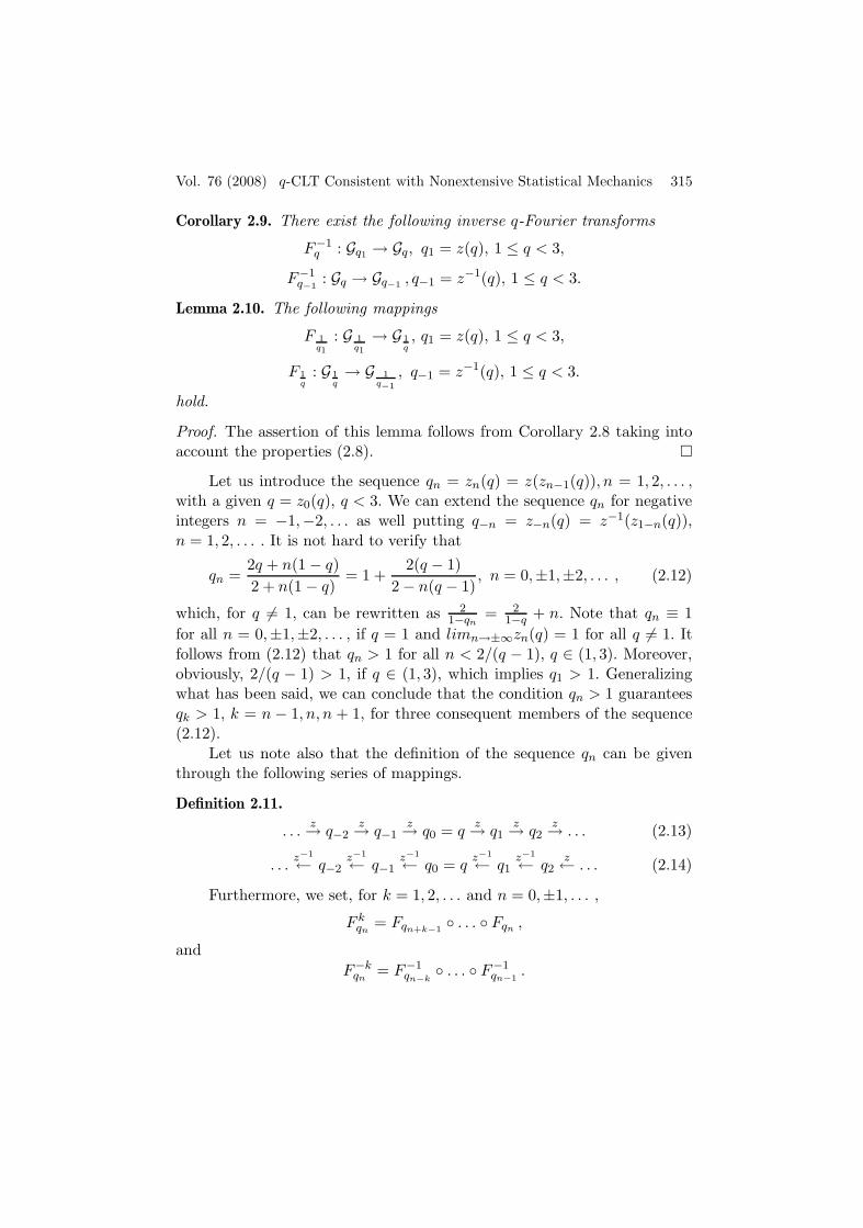
Corollary 2.9. There exist the following inverse q-Fourier transforms
F−1q : Gq1 → Gq, q1 = z(q), 1 ≤ q < 3,
F−1q−1
: Gq → Gq−1 , q−1 = z−1(q), 1 ≤ q < 3.
Lemma 2.10. The following mappings
F 1q1
: G 1q1
→ G 1q, q1 = z(q), 1 ≤ q < 3,
F 1q
: G 1q→ G 1
q−1
, q−1 = z−1(q), 1 ≤ q < 3.
hold.
Proof. The assertion of this lemma follows from Corollary 2.8 taking intoaccount the properties (2.8).
Let us introduce the sequence qn = zn(q) = z(zn−1(q)), n = 1, 2, . . . ,with a given q = z0(q), q < 3. We can extend the sequence qn for negativeintegers n = −1,−2, . . . as well putting q−n = z−n(q) = z−1(z1−n(q)),n = 1, 2, . . . . It is not hard to verify that
qn =2q + n(1− q)2 + n(1− q)
= 1 +2(q − 1)
2− n(q − 1), n = 0,±1,±2, . . . , (2.12)
which, for q = 1, can be rewritten as 21−qn
= 21−q + n. Note that qn ≡ 1
for all n = 0,±1,±2, . . . , if q = 1 and limn→±∞zn(q) = 1 for all q = 1. Itfollows from (2.12) that qn > 1 for all n < 2/(q − 1), q ∈ (1, 3). Moreover,obviously, 2/(q − 1) > 1, if q ∈ (1, 3), which implies q1 > 1. Generalizingwhat has been said, we can conclude that the condition qn > 1 guaranteesqk > 1, k = n − 1, n, n + 1, for three consequent members of the sequence(2.12).
Let us note also that the definition of the sequence qn can be giventhrough the following series of mappings.
Definition 2.11.
. . .z→ q−2
z→ q−1z→ q0 = q
z→ q1z→ q2
z→ . . . (2.13)
. . .z−1← q−2
z−1← q−1z−1← q0 = q
z−1← q1z−1← q2
z← . . . (2.14)
Furthermore, we set, for k = 1, 2, . . . and n = 0,±1, . . . ,
F kqn
= Fqn+k−1 . . . Fqn ,
andF−k
qn= F−1
qn−k . . . F−1
qn−1.
316 Umarov, Tsallis and Steinberg Vol. 76 (2008)
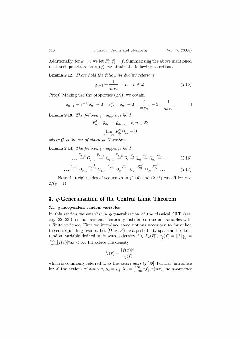
Additionally, for k = 0 we let F 0q [f ] = f. Summarizing the above mentioned
relationships related to zn(q), we obtain the following assertions.
Lemma 2.12. There hold the following duality relations
qn−1 +1
qn+1= 2, n ∈ Z. (2.15)
Proof. Making use the properties (2.9), we obtain
qn−1 = z−1(qn) = 2− z(2− qn) = 2− 1z(qn)
= 2− 1qn+1
.
Lemma 2.13. The following mappings hold:
F kqn
: Gqn → Gqk+n, k, n ∈ Z;
limk→−∞
F kqnGqn = G
where G is the set of classical Gaussians.
Lemma 2.14. The following mappings hold:
. . .Fq−3→ Gq−2
Fq−2→ Gq−1
Fq−2→ GqFq→ Gq1
Fq1→ Gq2
Fq2→ . . . (2.16)
. . .F−1
q−3← Gq−2
F−1q−2← Gq−1
F−1q−1← Gq
F−1q← Gq1
F−1q1← Gq2
F−1q2← . . . (2.17)
Note that right sides of sequences in (2.16) and (2.17) cut off for n ≥2/(q − 1).
3. q-Generalization of the Central Limit Theorem
3.1. q-independent random variables
In this section we establish a q-generalization of the classical CLT (see,e.g. [22, 23]) for independent identically distributed random variables witha finite variance. First we introduce some notions necessary to formulatethe corresponding results. Let (Ω,F , P ) be a probability space and X be arandom variable defined on it with a density f ∈ Lq(R), νq(f) = ‖f‖qLq
=∫∞−∞[f(x)]qdx <∞. Introduce the density
fq(x) =[f(x)]q
νq(f),
which is commonly referred to as the escort density [30]. Further, introducefor X the notions of q-mean, µq = µq(X) =
∫∞−∞ xfq(x) dx, and q-variance

Vol. 76 (2008) q-CLT Consistent with Nonextensive Statistical Mechanics 317
σ2q = σ2
q (X − µq) =∫∞−∞(x− µq)2fq(x) dx, subject to the integrals used in
these definitions to converge.The formulas below can be verified directly.
Lemma 3.1. The following formulas hold true1. µq(aX) = aµq(X);2. µq(X − µq(X)) = 0;3. σ2
q (aX) = a2σ2q (X).
Further, we introduce the notions of q-independence and q-convergence.
Definition 3.2. Two random variables X1 and Y1 are said to be
1. q-independent of first type if
Fq[X + Y ](ξ) = Fq[X](ξ) ⊗q Fq[Y ](ξ), (3.1)
2. q-independent of second type if
Fq−1 [X + Y ](ξ) = Fq−1 [X](ξ) ⊗q Fq−1[Y ](ξ), q = z(q−1), (3.2)
3. q-independent of third type if
Fq−1 [X + Y ](ξ) = Fq[X](ξ) ⊗q Fq[Y ](ξ), q = z(q−1), (3.3)
where X = X1 − µq(X1), Y = Y1 − µq(Y1).
All three types of q-independence generalize the classic notion of in-dependence. Namely, for q = 1 the conditions (3.1)-(3.3) turn into the wellknown relation
F [fX ∗ fY ] = F [fX ] · F [fY ]
between the convolution (noted ∗) of two densities and the multiplicationof their (classical) Fourier images, and holds for independent X and Y . Ifq = 1, then q-independence of a certain type describes a specific correlation.The relations (3.1)-(3.3) can be rewritten in terms of densities. Let fX andfY be densities of X and Y respectively, and let fX+Y be the density ofX + Y . Then, for instance, the q-independence of second type takes theform
∫ ∞
−∞eixξq−1⊗q−1 fX+Y (x)dx = Fq−1 [fX ](ξ)⊗q Fq−1 [fY ](ξ). (3.4)
Consider an example of q-independence of second type. Let random vari-ables X and Y have q-Gaussian densities Gq−1(β1, x) and Gq−1(β2, x) re-spectively. Denote γj = 3−q−1
8β2−q−1j C
2(q−1−1)q−1
, j = 1, 2. If X + Y is distributed
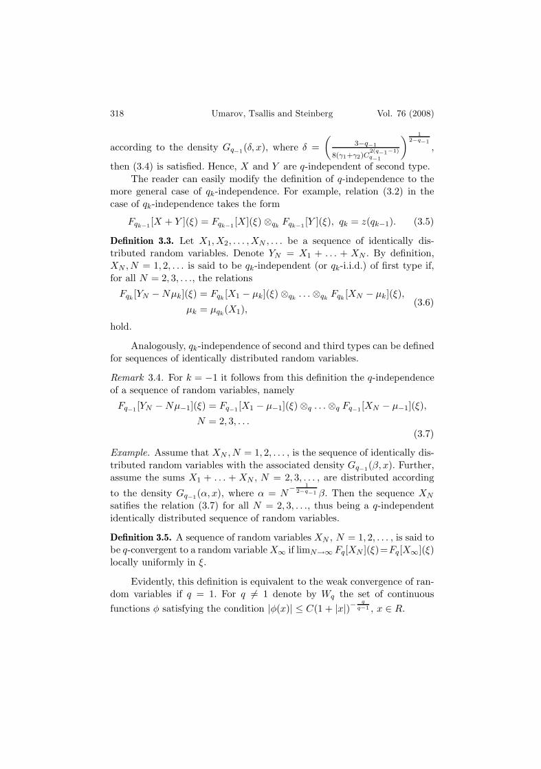
318 Umarov, Tsallis and Steinberg Vol. 76 (2008)
according to the density Gq−1(δ, x), where δ =(
3−q−1
8(γ1+γ2)C2(q−1−1)q−1
) 12−q−1
,
then (3.4) is satisfied. Hence, X and Y are q-independent of second type.The reader can easily modify the definition of q-independence to the
more general case of qk-independence. For example, relation (3.2) in thecase of qk-independence takes the form
Fqk−1[X + Y ](ξ) = Fqk−1
[X](ξ) ⊗qkFqk−1
[Y ](ξ), qk = z(qk−1). (3.5)
Definition 3.3. Let X1,X2, . . . ,XN , . . . be a sequence of identically dis-tributed random variables. Denote YN = X1 + . . . + XN . By definition,XN , N = 1, 2, . . . is said to be qk-independent (or qk-i.i.d.) of first type if,for all N = 2, 3, . . ., the relations
Fqk[YN −Nµk](ξ) = Fqk
[X1 − µk](ξ)⊗qk. . . ⊗qk
Fqk[XN − µk](ξ),
µk = µqk(X1),
(3.6)
hold.
Analogously, qk-independence of second and third types can be definedfor sequences of identically distributed random variables.
Remark 3.4. For k = −1 it follows from this definition the q-independenceof a sequence of random variables, namely
Fq−1[YN −Nµ−1](ξ) = Fq−1 [X1 − µ−1](ξ)⊗q . . .⊗q Fq−1 [XN − µ−1](ξ),
N = 2, 3, . . .(3.7)
Example. Assume that XN , N = 1, 2, . . . , is the sequence of identically dis-tributed random variables with the associated density Gq−1(β, x). Further,assume the sums X1 + . . . + XN , N = 2, 3, . . . , are distributed according
to the density Gq−1(α, x), where α = N− 1
2−q−1 β. Then the sequence XN
satifies the relation (3.7) for all N = 2, 3, . . ., thus being a q-independentidentically distributed sequence of random variables.
Definition 3.5. A sequence of random variables XN , N = 1, 2, . . . , is said tobe q-convergent to a random variable X∞ if limN→∞ Fq[XN ](ξ)=Fq[X∞](ξ)locally uniformly in ξ.
Evidently, this definition is equivalent to the weak convergence of ran-dom variables if q = 1. For q = 1 denote by Wq the set of continuousfunctions φ satisfying the condition |φ(x)| ≤ C(1 + |x|)− q
q−1 , x ∈ R.
Vol. 76 (2008) q-CLT Consistent with Nonextensive Statistical Mechanics 319
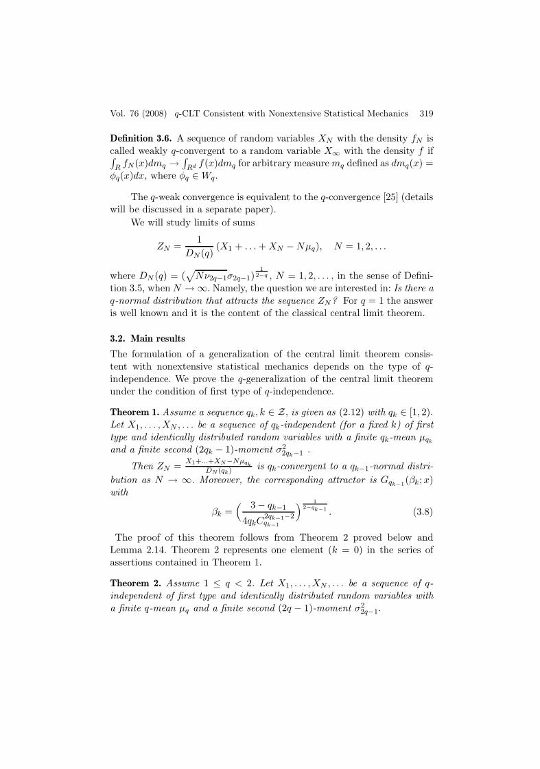
Definition 3.6. A sequence of random variables XN with the density fN iscalled weakly q-convergent to a random variable X∞ with the density f if∫R fN(x)dmq →
∫Rd f(x)dmq for arbitrary measure mq defined as dmq(x) =
φq(x)dx, where φq ∈Wq.
The q-weak convergence is equivalent to the q-convergence [25] (detailswill be discussed in a separate paper).
We will study limits of sums
ZN =1
DN (q)(X1 + . . . + XN −Nµq), N = 1, 2, . . .
where DN (q) = (√
Nν2q−1σ2q−1)1
2−q , N = 1, 2, . . . , in the sense of Defini-tion 3.5, when N →∞. Namely, the question we are interested in: Is there aq-normal distribution that attracts the sequence ZN? For q = 1 the answeris well known and it is the content of the classical central limit theorem.
3.2. Main results
The formulation of a generalization of the central limit theorem consis-tent with nonextensive statistical mechanics depends on the type of q-independence. We prove the q-generalization of the central limit theoremunder the condition of first type of q-independence.
Theorem 1. Assume a sequence qk, k ∈ Z, is given as (2.12) with qk ∈ [1, 2).Let X1, . . . ,XN , . . . be a sequence of qk-independent (for a fixed k) of firsttype and identically distributed random variables with a finite qk-mean µqk
and a finite second (2qk − 1)-moment σ22qk−1 .
Then ZN = X1+...+XN−NµqkDN (qk) is qk-convergent to a qk−1-normal distri-
bution as N → ∞. Moreover, the corresponding attractor is Gqk−1(βk;x)
with
βk =( 3− qk−1
4qkC2qk−1−2qk−1
) 12−qk−1 . (3.8)
The proof of this theorem follows from Theorem 2 proved below andLemma 2.14. Theorem 2 represents one element (k = 0) in the series ofassertions contained in Theorem 1.
Theorem 2. Assume 1 ≤ q < 2. Let X1, . . . ,XN , . . . be a sequence of q-independent of first type and identically distributed random variables witha finite q-mean µq and a finite second (2q − 1)-moment σ2
2q−1.
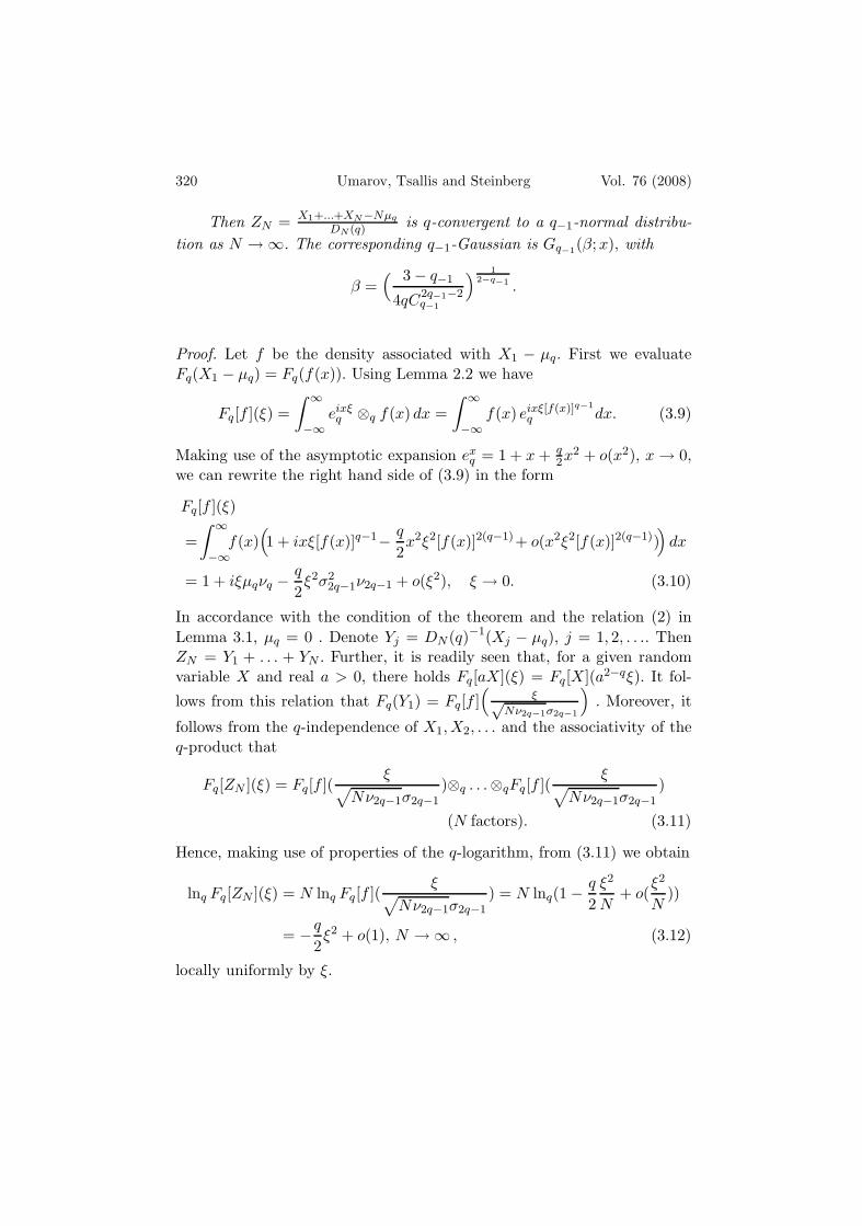
320 Umarov, Tsallis and Steinberg Vol. 76 (2008)
Then ZN = X1+...+XN−Nµq
DN (q) is q-convergent to a q−1-normal distribu-tion as N →∞. The corresponding q−1-Gaussian is Gq−1(β;x), with
β =( 3− q−1
4qC2q−1−2q−1
) 12−q−1 .
Proof. Let f be the density associated with X1 − µq. First we evaluateFq(X1 − µq) = Fq(f(x)). Using Lemma 2.2 we have
Fq[f ](ξ) =∫ ∞
−∞eixξq ⊗q f(x) dx =
∫ ∞
−∞f(x) eixξ[f(x)]q−1
q dx. (3.9)
Making use of the asymptotic expansion exq = 1 + x + q
2x2 + o(x2), x→ 0,we can rewrite the right hand side of (3.9) in the form
Fq[f ](ξ)
=∫ ∞
−∞f(x)
(1 + ixξ[f(x)]q−1− q
2x2ξ2[f(x)]2(q−1)+ o(x2ξ2[f(x)]2(q−1))
)dx
= 1 + iξµqνq − q
2ξ2σ2
2q−1ν2q−1 + o(ξ2), ξ → 0. (3.10)
In accordance with the condition of the theorem and the relation (2) inLemma 3.1, µq = 0 . Denote Yj = DN (q)−1(Xj − µq), j = 1, 2, . . .. ThenZN = Y1 + . . . + YN . Further, it is readily seen that, for a given randomvariable X and real a > 0, there holds Fq[aX](ξ) = Fq[X](a2−qξ). It fol-
lows from this relation that Fq(Y1) = Fq[f ](
ξ√Nν2q−1σ2q−1
). Moreover, it
follows from the q-independence of X1,X2, . . . and the associativity of theq-product that
Fq[ZN ](ξ) = Fq[f ](ξ
√Nν2q−1σ2q−1
)⊗q . . .⊗qFq[f ](ξ
√Nν2q−1σ2q−1
)
(N factors). (3.11)
Hence, making use of properties of the q-logarithm, from (3.11) we obtain
lnq Fq[ZN ](ξ) = N lnq Fq[f ](ξ
√Nν2q−1σ2q−1
) = N lnq(1− q
2ξ2
N+ o(
ξ2
N))
= −q
2ξ2 + o(1), N →∞ , (3.12)
locally uniformly by ξ.
Vol. 76 (2008) q-CLT Consistent with Nonextensive Statistical Mechanics 321
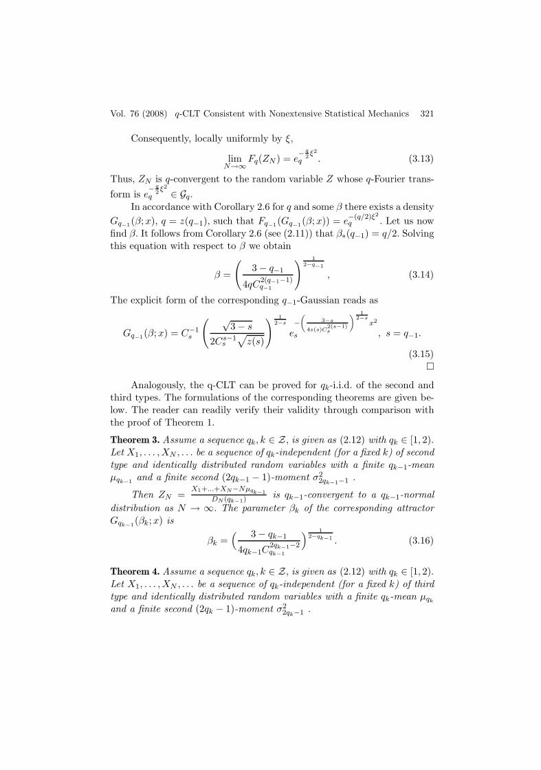
Consequently, locally uniformly by ξ,
limN→∞
Fq(ZN ) = e− q
2ξ2
q . (3.13)
Thus, ZN is q-convergent to the random variable Z whose q-Fourier trans-
form is e− q
2ξ2
q ∈ Gq.In accordance with Corollary 2.6 for q and some β there exists a density
Gq−1(β;x), q = z(q−1), such that Fq−1(Gq−1(β;x)) = e−(q/2)ξ2
q . Let us nowfind β. It follows from Corollary 2.6 (see (2.11)) that β∗(q−1) = q/2. Solvingthis equation with respect to β we obtain
β =
(3− q−1
4qC2(q−1−1)q−1
) 12−q−1
, (3.14)
The explicit form of the corresponding q−1-Gaussian reads as
Gq−1(β;x) = C−1s
( √3− s
2Cs−1s
√z(s)
) 12−s
e−(
3−s
4z(s)C2(s−1)s
) 12−s
x2
s , s = q−1.
(3.15)
Analogously, the q-CLT can be proved for qk-i.i.d. of the second andthird types. The formulations of the corresponding theorems are given be-low. The reader can readily verify their validity through comparison withthe proof of Theorem 1.
Theorem 3. Assume a sequence qk, k ∈ Z, is given as (2.12) with qk ∈ [1, 2).Let X1, . . . ,XN , . . . be a sequence of qk-independent (for a fixed k) of secondtype and identically distributed random variables with a finite qk−1-meanµqk−1
and a finite second (2qk−1 − 1)-moment σ22qk−1−1 .
Then ZN =X1+...+XN−Nµqk−1
DN (qk−1)is qk−1-convergent to a qk−1-normal
distribution as N → ∞. The parameter βk of the corresponding attractorGqk−1
(βk;x) is
βk =( 3− qk−1
4qk−1C2qk−1−2qk−1
) 12−qk−1 . (3.16)
Theorem 4. Assume a sequence qk, k ∈ Z, is given as (2.12) with qk ∈ [1, 2).Let X1, . . . ,XN , . . . be a sequence of qk-independent (for a fixed k) of thirdtype and identically distributed random variables with a finite qk-mean µqk
and a finite second (2qk − 1)-moment σ22qk−1 .

322 Umarov, Tsallis and Steinberg Vol. 76 (2008)
Then ZN = X1+...+XN−NµqkDN (qk) is qk−1-convergent to a qk−1-normal dis-
tribution as N →∞. Moreover, the corresponding attractor Gqk−1(βk;x) in
this case is the same as in the Theorem 1 with βk given in (3.8).
Obviously, q+13−q = 1 if and only if q = 1. This fact yields the following
corollary.
Corollary 3.7. Let X1, . . . ,XN , . . . be a given sequence of qk-independent(of any type) random variables satisfying the corresponding conditions ofTheorems 1–3. Then the attractor of ZN is a qk-normal distribution if andonly if qk = 1, that is, in the classic case.
4. Conclusion
In the present paper we studied q-generalizations of the classic central limittheorem adapted to nonextensive statistical mechanics, depending on threetypes of correlation. Interrelation showing the dependence of a type of con-vergence to a q-Gaussian on a type of correlation is summarized in Table1.
Table 1. Interrelation between the type of correlation, con-ditions for q-mean and q-variance, type of convergence, andparameter of the attractor
Corr. type Conditions Convergence Gaussian parameter
1st type µqk<∞, qk − conv. βk =
(3−qk−1
4qkC2qk−1−2qk−1
) 12−qk−1
σ22qk−1 <∞
2nd type µqk−1 <∞, qk−1 − conv. βk =(
3−qk−1
4qk−1C2qk−1−2qk−1
) 12−qk−1
σ22qk−1−1 <∞
3rd type µqk<∞, qk−1 − conv. βk =
(3−qk−1
4qkC2qk−1−2qk−1
) 12−qk−1
σ22qk−1 <∞
In all three cases the corresponding attractor is distributed accordingto a qk−1-normal distribution, where qk−1 = z−1(qk). We have noticed thatqk = qk−1 if qk = 1. In the classic case both qk = 1 and z−1(qk) = 1, sothat the corresponding Gaussians do not differ. So, Corollary 3.7 notes thatsuch duality is a specific feature of the nonextensive statistical theory, which
Vol. 76 (2008) q-CLT Consistent with Nonextensive Statistical Mechanics 323
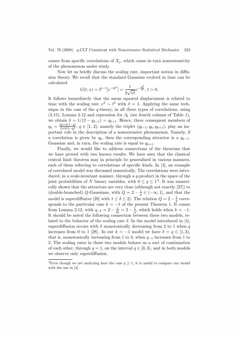
comes from specific correlations of Xj, which cause in turn nonextensivityof the phenomenon under study.
Now let us briefly discuss the scaling rate, important notion in diffu-sion theory. We recall that the standard Gaussian evolved in time can becalculated
G(t, x) = F−1[e−tξ2] =
12√
πte−
x2
4t , t > 0.
It follows immediately that the mean squared displacement is related totime with the scaling rate x2 ∼ tδ with δ = 1. Applying the same tech-nique in the case of the q-theory, in all three types of correlations, using(3.15), Lemma 2.12 and expression for βk (see fourth column of Table 1),we obtain δ = 1/(2 − qk−1) = qk+1. Hence, three consequent members ofqk = 2q+k(1−q)
2+k(1−q) , q ∈ [1, 2), namely the triplet (qk−1, qk, qk+1), play an im-portant role in the description of a nonextensive phenomenon. Namely, ifa correlation is given by qk, then the corresponding attractor is a qk−1-Gaussian and, in turn, the scaling rate is equal to qk+1.
Finally, we would like to address connections of the theorems thatwe have proved with two known results. We have seen that the classicalcentral limit theorem may in principle be generalized in various manners,each of them referring to correlations of specific kinds. In [4], an exampleof correlated model was discussed numerically. The correlations were intro-duced, in a scale-invariant manner, through a q-product in the space of thejoint probabilities of N binary variables, with 0 ≤ q ≤ 1 3. It was numeri-cally shown that the attractors are very close (although not exactly [27]) to(double-branched) Q-Gaussians, with Q = 2 − 1
q ∈ (−∞, 1], and that themodel is superdiffusive [28] with 1 ≤ δ ≤ 2). The relation Q = 2− 1
q corre-sponds to the particular case k = −1 of the present Theorem 1. It comesfrom Lemma 2.12, with q−2 = 2 − 1
q0= 2 − 1
q , which holds when k = −1.It should be noted the following connection between these two models, re-lated to the behavior of the scaling rate δ. In the model introduced in [4],superdiffusion occurs with δ monotonically decreasing from 2 to 1 when qincreases from 0 to 1 [28] . In our k = −1 model we have δ = q ∈ [1, 3),that is, monotonically increasing from 1 to 3, when q−1 increases from 1 to2. The scaling rates in these two models behave as a sort of continuationof each other, through q = 1, on the interval q ∈ [0, 3), and in both modelswe observe only superdiffusion.
3Even though we are analyzing here the case q ≥ 1, it is useful to compare our model
with the one in [4].
324 Umarov, Tsallis and Steinberg Vol. 76 (2008)
Another example is suggested by the exact stable solutions of a nonlin-ear Fokker-Planck equation in [6]. The correlations4 are introduced througha q = 2 − Q exponent in the spatial member of the equation (the secondderivative term). The solutions are Q-Gaussians with Q ∈ (−∞, 3), andδ = 2/(3 − Q) ∈ [0,∞], hence both superdiffusion and subdiffusion canexist in addition to normal diffusion. This model is particularly interest-ing because the scaling δ = 2/(3 − Q) was conjectured in [31], and it wasverified in various experimental and computational studies [32, 33, 34, 35].
In the particular case of Theorem 1, k = 1, we have δ = q2 = 1/(2−q).This result coincides with that of the nonlinear Fokker-Planck equationmentioned above. Indeed, in our theorem (k = 1) we require the finitnessof (2q−1)-variance. Denoting 2q−1 = Q, we get δ = 1/(2−q) = 2/(3−Q).Notice, however, that this example differs from the nonlinear Fokker-Planckabove. Indeed, although we do obtain, from the finiteness of the secondmoment, the same expression for δ, the attractor is not a Q-Gaussian, butrather a Q+1
2 -Gaussian.Summarizing, the present Theorems 1–4 suggest a quite general and
rich structure at the basis of nonextensive statistical mechanics. Moreover,they recover, as particular instances, central relations emerging in the abovetwo examples. The structure we have presently shown might pave a deepunderstanding of the so-called q-triplet (qsen, qrel, qstat), where sen, rel andstat respectively stand for sensitivity to the initial conditions, relaxation,and stationary state [36, 37, 38] in nonextensive statistics. This remainshowever as a challenge at the present stage. Another open question – veryrelevant in what concerns physical applications – refers to whether the q-independence addressed here reflects a sort of asymptotic scale-invarianceas N increases.
Acknowledgments
We acknowledge thoughtful remarks by K. Chow, M. Gell-Mann, M.G.Hahn, R. Hersh, J.A. Marsh, R.S. Mendes, L.G. Moyano, S.M.D. Queirosand W. Thistleton. One of us (CT) has benefited from lengthy conversationson the subject with M. Gell-Mann and D. Prato. Financial support by theFullbright Foundation, NIH grant P20 GMO67594, SI International andAFRL (USA), and by CNPq and Faperj (Brazil) is acknowledged as well.
4The correlation defined in [6] is different from the q-independence of types 1-3 introduced
in this paper.
Vol. 76 (2008) q-CLT Consistent with Nonextensive Statistical Mechanics 325
References
[1] C. Tsallis, Possible generalization of Boltzmann-Gibbs statistics, J. Stat.Phys. 52, 479 (1988). See also E.M.F. Curado and C. Tsallis, Generalizedstatistical mechanics: connection with thermodynamics, J. Phys. A 24, L69(1991) [Corrigenda: 24, 3187 (1991) and 25, 1019 (1992)], and C. Tsallis,R.S. Mendes and A.R. Plastino, The role of constraints within generalizednonextensive statistics, Physica A 261, 534 (1998).
[2] C. Tsallis, Nonextensive statistical mechanics, anomalous diffusion and cen-tral limit theorems, Milan Journal of Mathematics 73, 145 (2005).
[3] D. Prato and C. Tsallis, Nonextensive foundation of Levy distributions,Phys. Rev. E 60, 2398 (1999), and references therein.
[4] L.G. Moyano, C. Tsallis and M. Gell-Mann, Numerical indications of aq-generalised central limit theorem, Europhys. Lett. 73, 813 (2006).
[5] G. Jona-Lasinio, The renormalization group: A probabilistic view, NuovoCimento B 26, 99 (1975), and Renormalization group and probability the-ory, Phys. Rep. 352, 439 (2001), and references therein; P.A. Mello and B.Shapiro, Existence of a limiting distribution for disordered electronic con-ductors, Phys. Rev. B 37, 5860 (1988); P.A. Mello and S. Tomsovic, Scat-tering approach to quantum electronic transport, Phys. Rev. B 46, 15963(1992); M. Bologna, C. Tsallis and P. Grigolini,Anomalous diffusion associ-ated with nonlinear fractional derivative Fokker-Planck-like equation: Exacttime-dependent solutions, Phys. Rev. E 62, 2213 (2000); C. Tsallis, C. An-teneodo, L. Borland and R. Osorio, Nonextensive statistical mechanics andeconomics, Physica A 324, 89 (2003); C. Tsallis, What should a statisticalmechanics satisfy to reflect nature?, in Anomalous Distributions, NonlinearDynamics and Nonextensivity, eds. H.L. Swinney and C. Tsallis, Physica D193, 3 (2004); C. Anteneodo, Non-extensive random walks, Physica A 358,289 (2005); S. Umarov and R. Gorenflo, On multi-dimensional symmetricrandom walk models approximating fractional diffusion processes, FractionalCalculus and Applied Analysis 8, 73-88 (2005); S. Umarov and S. Steinberg,Random walk models associated with distributed fractional order differentialequations, to appear in IMS Lecture Notes - Monograph Series; F. Bal-dovin and A. Stella, Central limit theorem for anomalous scaling due tocorrelations, Phys. Rev. E 75, 020101 (2007); C. Tsallis, On the extensivityof the entropy Sq, the q-generalized central limit theorem and the q-triplet,in Proc. International Conference on Complexity and Nonextensivity: NewTrends in Statistical Mechanics (Yukawa Institute for Theoretical Physics,Kyoto, 14-18 March 2005), eds. S. Abe, M. Sakagami and N. Suzuki, Prog.Theor. Phys. Supplement 162, 1 (2006); D. Sornette, Critical Phenomenain Natural Sciences (Springer, Berlin, 2001), page 36.
326 Umarov, Tsallis and Steinberg Vol. 76 (2008)
[6] C. Tsallis and D.J. Bukman, Anomalous diffusion in the presence of exter-nal forces: exact time-dependent solutions and their thermostatistical basis,Phys. Rev. E 54, R2197 (1996).
[7] K. Yoshihara, Weakly dependent stochastic sequences and their applications,V.1. Summation theory for weakly dependent sequences (Sanseido, Tokyo,1992).
[8] M. Peligrad, Recent advances in the central limit theorem and its weak in-variance principle for mixing sequences of random variables (a survey), inDependence in probability and statistics, eds. E. Eberlein and M.S.Taqqu,Progress in Probability and Statistics 11, 193 (Birkhaser, Boston, 1986).
[9] E. Rio, Theorie asymptotique des processus aleatoires faiblement depen-dants, Mathematiques et Applications 31 (Springer, Berlin, 2000).
[10] P. Doukhan, Mixing properties and examples, Lecture Notes in Statistics 85
(1994).[11] H. Dehling, M. Denker and W. Philipp, Central limit theorem for mixing
sequences of random variables under minimal condition, Annals of Proba-bility 14 (4), 1359 (1986).
[12] R.C. Bradley, Introduction to strong mixing conditions, V I,II, Technical re-port, Department of Mathematics, Indiana University, Bloomington (Cus-tom Publishing of IU, 2002-2003).
[13] H.G. Dehling, T. Mikosch and M. Sorensen, eds., Empirical process tech-niques for dependent data (Birkhaser, Boston-Basel-Berlin, 2002).
[14] L. Euler, Introductio in Analysin Infinitorum, T. 1, Chapter XVI, p. 259,Lausanne, 1748.
[15] F. H. Jackson, On q-Functions and a Certain Difference Operator, Trans.Roy Soc. Edin. 46 (1908), 253281.
[16] T. Ernst, A method for q-calculus, Journal of Nonlinear MathematicalPhysics Volume 10, Number 4 (2003), 487525
[17] C. Tsallis, M. Gell-Mann and Y. Sato, Asymptotically scale-invariant occu-pancy of phase space makes the entropy Sq extensive, Proc. Natl. Acad. Sc.USA 102, 15377 (2005).
[18] C. Tsallis, What are the numbers that experiments provide ?, Quimica Nova17, 468 (1994).
[19] M. Gell-Mann and C. Tsallis, eds., Nonextensive Entropy - InterdisciplinaryApplications (Oxford University Press, New York, 2004).
[20] L. Nivanen, A. Le Mehaute and Q.A. Wang, Generalized algebra within anonextensive statistics, Rep. Math. Phys. 52, 437 (2003).
[21] E.P. Borges, A possible deformed algebra and calculus inspired in nonexten-sive thermostatistics, Physica A 340, 95 (2004).
Vol. 76 (2008) q-CLT Consistent with Nonextensive Statistical Mechanics 327
[22] P. Billingsley. Probability and Measure. John Wiley and Sons, 1995.[23] R. Durrett. Probability: Theory and Examples. Thomson, 2005.[24] J. Marsh and S. Earl, New solutions to scale-invariant phase-space occu-
pancy for the generalized entropy Sq, Phys. Lett. A 349, 146-152 (2005).[25] S. Umarov and C. Tsallis, Multivariate Generalizations of the q-Central
Limit Theorem, cond-mat/0703533 (2007).[26] C. Tsallis, M. Gell-Mann and Y. Sato, Extensivity and entropy production,
Europhysics News 36, 186 (2005).[27] H.J. Hilhorst and G. Schehr, A note on q-Gaussians and non-Gaussians in
statistical mechanics, J. Stat. Mech. P06003 (2007).[28] J.A. Marsh, M.A. Fuentes, L.G. Moyano and C. Tsallis, Influence of global
correlations on central limit theorems and entropic extensivity, Physica A372, 183 (2006).
[29] F. Caruso and C. Tsallis, Extensive nonadditive entropy in quantum spinchains, in Complexity, Metastability and Nonextensivity, eds. S. Abe, H.J.Herrmann, P. Quarati, A. Rapisarda and C. Tsallis, American Institute ofPhysics Conference Proceedings 965, 51 (New York, 2007).
[30] C. Beck and F. Schlogel, Thermodynamics of Chaotic Systems: An Intro-duction (Cambridge University Press, Cambridge, 1993).
[31] C. Tsallis, Some thoughts on theoretical physics, Physica A 344, 718 (2004).[32] A. Upadhyaya, J.-P. Rieu, J.A. Glazier and Y. Sawada, Anomalous diffusion
and non-Gaussian velocity distribution of Hydra cells in cellular aggregates,Physica A 293, 549 (2001).
[33] K.E. Daniels, C. Beck and E. Bodenschatz, Defect turbulence and general-ized statistical mechanics, in Anomalous Distributions, Nonlinear Dynamicsand Nonextensivity, eds. H.L. Swinney and C. Tsallis, Physica D 193, 208(2004).
[34] A. Rapisarda and A. Pluchino, Nonextensive thermodynamics and glassybehavior, Europhysics News 36, 202 (2005).
[35] R. Arevalo, A. Garcimartin and D. Maza, Anomalous diffusion in silodrainage, Eur. Phys. J. E 23, 191 (2007).
[36] C. Tsallis, Dynamical scenario for nonextensive statistical mechanics, inNews and Expectations in Thermostatistics, eds. G. Kaniadakis and M.Lissia, Physica A 340, 1 (2004).
[37] L.F. Burlaga and A.F. Vinas, Triangle for the entropic index q of non-extensive statistical mechanics observed by Voyager 1 in the distant helio-sphere, Physica A 356, 375 (2005).
[38] L.F. Burlaga, A.F. Vinas, N.F. Ness and M.H. Acuna, Tsallis statistics ofmagnetic field in heliosheath, Astrophys. J. Lett. 644, L83 (2006).
328 Umarov, Tsallis and Steinberg Vol. 76 (2008)
Sabir UmarovDepartment of MathematicsTufts UniversityMedford, MA 02155USAe-mail: [email protected]
Constantino TsallisCentro Brasileiro de Pesquisas FisicasXavier Sigaud 15022290-180 Rio de Janeiro-RJBrazilandSanta Fe Institute1399 Hyde Park RoadSanta Fe, NM 87501USAe-mail: [email protected]
Stanly SteinbergDepartment of Mathematics and StatisticsUniversity of New MexicoAlbuquerque, NM 87131USAe-mail: [email protected]
Received: November 2007