on a new type of mixed interpolation - core.ac.uk h. de meyer et al. / mixed interpolation by...

Journal of Computational and Applied Mathematics 30 (1990) 55-69 North-Holland

55

On a new type of mixed interpolation

H. DE MEYER, J. VANTHOURNOUT and G. VANDEN BERGHE Laboratorium voor Numerieke Wiskunde en Informatica, Rijksuniversiteit Gent, KrijgsIaan 281 -S9, B9000 Gent, Belgium

Received 3 February 1989 Revised 8 June 1989

Abstract: We approximate every function f by a function f,,(x) of the form a cos kx + b sin kx +C~&x’ so that f(jh) = f,(jh) for the n + 1 equidistant points jh, j = 0,. .., n. That interpolation function f,(x) is proved to be unique and can be written as the sum of the n th-degree interpolation polynomial based on the same points and two correction terms. The error term is also discussed. The results for this mixed type of interpolation reduce to the known results of the polynomial case as the parameter k is tending to 0. This new interpolation theory will be used in the future for the construction of quadrature rules and multistep methods for ordinary differential equations.

Keywords: Interpolation function, mixed and polynomial interpolation, error term, forward and backward differences.

1. Introduction

There are many numerical methods available for numerical integration and for the step-by-step integration of ordinary differential equations. Only few of them, however, take advantage of either the special behaviour of occurring integrands or of special properties of the ODE solution that may be known in advance.

The numerical computation of integrals of the type

where f(x) has a simple periodic behaviour, is generally carried out by means of Filon’s formula [2,4] or generalizations thereof [5,8,14]. For the more general case where f(x) has more complex periodic properties more sophisticated methods are required. One such has been devised by Levin [7]. A survey of other available methods can be found in [2]. Very recently, Ehrenmark [3] introduced a new quadrature formula which exactly integrates the functions 1, sin kx and cos kx

over an interval [0, 2h]. Herein k denotes the frequency of the periodic integrand and h denotes the considered step. In fact this method is an adaptation of one of the classical Newton-Cotes quadrature formulas also called Simpson’s rule. These Newton-Cotes quadrature formulas are derived by replacing under the integral sign the integrand by a suitable interpolation polynomial of the Lagrange type with equally spaced nodes and by integrating afterwards. Ehrenmark’s formula can also be obtained by an analoguous operation. By replacing firstly the integrand f(x) by an interpolation function of the form a + b sin kx + c cos kx, reproducing f(x) exactly in the nodes 0, h and 2h and integrating afterwards, one obtains Ehrenmark’s formula. Moreover

0377-0427/90/$3.50 0 1990, Elsevier Science Publishers B.V. (North-Holland)

56 H. De Meyer et al. / Mixed interpolation

by studying the error term associated to the above-mentioned interpolant one obtains interesting information about the local truncation error of the proposed quadrature formula. Application shows that the formula is versatile and in particular extremely easy and fast to implement. Moreover a natural extension of other Newton-Cotes quadrature formulas along the same lines is worthwhile to investigate. Therefore a study of interpolation functions of the form

a sin kx + b cos kx + Q,_,(x), (1.2)

with Q,(x) an ordinary polynomial of degree m, and of its error term is important. Gautschi [6] constructed methods of Adams and Stijrmer type for problems with oscillatory

solutions. Neta and Ford [ll] developed Nystrom and generalized Milne-Simpson type methods. Other authors developed similar or analogous methods for this problem (see [1,9,10,13,15]). Most of the above methods consider initial-value problems of the type

ycr’(x)=f(x, y(x)), y’j’(a)=O, j=O,l,..., r-l, (1.3)

where Y is restricted to 1 or 2. One constructs the multistep method

i (yiYrz+i = ” i Pif Cxn+i7 Yn+i>, 0 -4

I=0 i=o

or, equivalently, the associated linear difference operator

L[y] = 2 “;y(x + ih) -h’; &y@‘(x + ih). (1.5) i=o i=o

By a suitable choice of the a;-coefficients and by requiring that

L[l] -0, L[cos jkx] =L[sin jkx] ~0, j= 1, 2 ,..., 4, (1.6) and

L [cos( q + 1) kx] and L [ sin( 4 + 1) kx] not both identically zero,

one obtains the above-mentioned methods of trigonometric order q relative to the frequency k.

Again it is worthwhile to study methods which integrate exactly functions of the type (1.2). In terms of the operator (1.5), one has to require that

and

L[x’] so, j=o, 1,2 )...) 2q-2, L[sin kx] = L[cos kx] =0 (1 J)

L[x~~-~] # 0 and L[sin 2kx] # 0, L[cos 2kx] # 0.

In particular for Y = 1 an alternative way, to obtain analogous results, consists in integrating (1.3) for r = 1 over a fixed interval. Since f (x, y(x)) cannot be integrated without knowing y(x), one can integrate an interpolation function of the form (1.2), that is determined by some of the previously obtained data points. Again local truncation errors for these multistep methods are related to the error term of the interpolation function considered. These kinds of multistep methods have been applied to the numerical solution of radial Schriidinger equations [12].

2. A mixed type of interpolation

We consider the problem of approximating a function f(x) by a certain combination of trigonometric and polynomial functions. More precisely, we replace f(x) by a function f,(x) of

H. De Meyer et al. / Mixed interpolation 57

the form n-2

f,(x) = a cos kx + b sin kx + c cixi, n 2 2, (2.1) i=O

whereby k is a real parameter which may be chosen freely so far. Also, we shall call n the order of the proposed interpolation function f,(x). Furthermore, we shall require that the error term defined as

Mf 7 4 :=f (4 -fnb), (2.2) vanishes at the n + 1 equidistant points xI = jh with j = 0, 1,. . . , n, h being a nonnegative real number, i.e.,

E,(f, jh)=O, VjE (0, l,..., n}. (2.3)

The n + 1 conditions (2.3) constitute a linear system of equations in the n + 1 coefficients a, b and ci, i=O, l,..., n - 2. In Appendix A it is shown that the determinant of the system, which we shall denote by A,, is given in closed form by the expression

A =.&"-1)("-2)/222n-1 n (2.4)

with

0 := hk.

It follows that on fulfilling the condition

(2.9

Vl E Z: 8 # 1~ or equivalently k # $, P-6)

a unique solution is guaranteed. Solving explicitly the system with respect to a, b and ci in terms of the function values f( jh) at the interpolation points seems an impossible task in general. However, by writing the solution for each of the coefficients formally as the ratio of two determinants, the denominator being A, and the numerator being obtained by the replacement of one column of the matrix of the system with the column [f (0) f(h) f (2h) . . . f (nh)]=, it is appropriate to recombine in the numerator rows in exactly the same way as was done for A, in Appendix A. In this way we obtain, at least formally, that

a = $ i (-1)P~,4f(ph)(A,)p+l,l, n p=o

b = $ k (-I)‘+’ vlf (~hkC,)p+~,2, n p=o

CiCf i (-qp+’ V,4f(ph)(An)p+,,i+3, i=O, l,...,n-2. n p=o

Herein (A,),,, is the determinant of the matrix which we obtain from the matrix [A] defined in (A.9) by leaving out the pth row and the qth column. Substituting this formal solution in (2.1) and recollecting terms in V,4f( ph), it is readily shown that f,(x) may be rewritten in the form

fnb) = k p$o$p+kd vLf(ph), (2.7)


whereby the x-dependent function .ES?‘~+~ (x) now represents the determinant of the matrix which is obtained by replacing in [A] the ( p + 1)th row with the row

[ cos kx sin kx 1 x x2 . . . xnp2].

In Appendix B it is proved that

J$+,(x)=A,(;), p=O,l,..., n-2,

with

s=X h'

P-8)

(2.9) showing that only two functions .E@‘,,( x) and ~$+t( x) remain to be determined in explicit form. At this intermediate step we already know that

f,(x) = ni2 (;) v,qf(ph) + f { K(x) vhn-lf((n - l)h) +4+,(x) Gfbh)} p=o n

(2.10)

and in the first part on the right-hand side we recognize the interpolation polynomial of degree n - 2 which coincides with f(x) in the n - 1 points xi, j = 0, 1,. . . , n - 2. Instead of calculating the remaining functions by means of their definition as a ratio of determinants, we shall make use of the fact that f,(x) is identical to f(x) in the cases that f(x) = sin kx or f(x) = cos kx. Making this observation explicit, we obtain from (2.10) two linear equations in .EC$(X) and .E$+~(x), namely:

V;-’ sin(n - 1)&c&(x) + 0; sin n&z@‘,,+,(x) =A, sin kx - ‘c*(i) vBp sin p9 I p=o

VI3 n-1 cos(n - l)f3J&(x) + VB” cos n&z$+,(x) =A, i coskx-n~2(;jv~cospe].

p=o

This system is easily solved and by substituting the solution into (2.10) we find

f,(x) = i*(i) Wf(d p=o

n-2

+ CC 1 p=o

i vi sin pt3 - sin kx v,” cos n0 1 vi cos p6 - cos kx $v;-‘f((n - l)h) n

\;7Sp cos pB - cos kx 1 v,"-' sin(n - l)e

- v,f sin pB- sin kx v,“-’ cos(n - l)f3 1 (2.11)


where D,, has been established in closed form in (A.14). Notice that the first term between braces

can be replaced by

and that in this expression the coefficient of (, :1) corresponds to the definition of D,,. In order to make notations more concise, let us introduce for all n 2 1 a function C&,(X) defined as

vBp cos pll-cos kx v,” sin nt9 1 - vBp sin pe-sin kx (2.12)

The reason why a factor k* has been introduced in the denominator will become clear further on. Making use of the property D,/D,_, = 4 sin*@, the function f,(x) may now be rewritten in the following form:

f,(x) = ni1 (;) 0,4f( PV - k*%(X) vhn-‘f((n - l)h) p=o

k* + 4 sin2~e%-‘(x) Cf(nQ (2.13)

Herein we recognize a first part which is the interpolation polynomial of (n - 1)th degree passing through the points (xi, f(xj)), j = 0, 1,. . . , n - 1, and two correction terms which involve the functions G,,(X) and $n_1(x). It is clear that the expression (2.12) is not very well suited for direct calculation of function values. In the following paragraphs we shall be concerned with the study of properties of the function C&(X) and at the same time we shall establish alternative expressions for the interpolation function f,(x).

3. Other forms of the interpolation function

By means of the formulae (A.12), (A.13) of Appendix A it is straightforward to show that:

v; cos ne -L[,;-2 D, = D,,-1

cos(n-2)e+~~-1~~~(~-1)e], vna2,

0,” sin ne -‘[v;-* sin(n-2)8+v,“-l sin(n-1)8] Vn>2

D,, = D,-1 2 , .

(3.1)

(3.2)

First separating on the right-hand side of (2.12) the two terms with p = n - 1 which on account of (A.ll) together yield the contribution (,i1)/k2, the use of (3.1) and (3.2) leads to the


intermediate result

1

-k2D,_, vJBP cos pB - cos kx v,“-’ sin(n - 2)0 1

-

u 1 p=o i vBp sin pe - sin kx v,“-~ cos( n - 2) 0 . 1 i

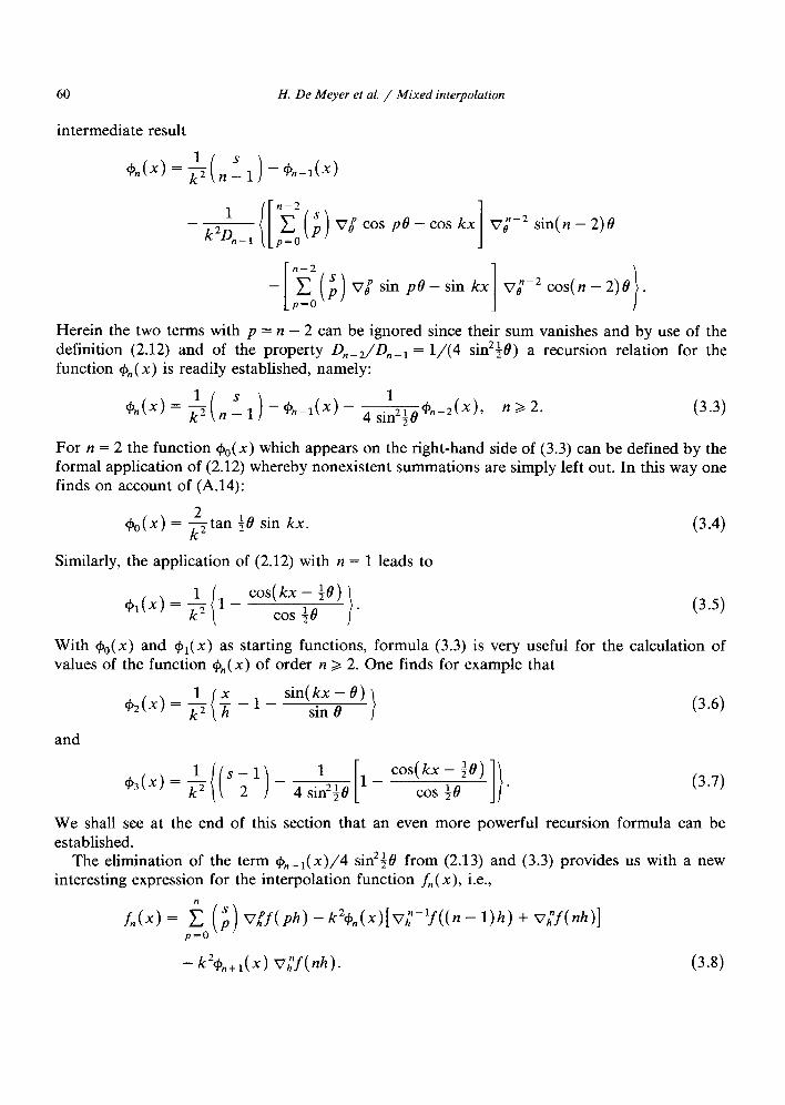
Herein the two terms with p = n - 2 can be ignored since their sum vanishes and by use of the definition (2.12) and of the property Dn_2/Dn_1 = l/(4 sin=@) a recursion relation for the function &(x) is readily established, namely:

For n = 2 the function +o(~) which appears on the right-hand side of (3.3) can be defined by the formal application of (2.12) whereby nonexistent summations are simply left out. In this way one finds on account of (A.14):

Go(x) = Stan ie sin kx.

Similarly, the application of (2.12) with n = 1 leads to

(3.4)

cos( kx - :O)

cos :e . (3.5)

With c#B~(x) and @J,(X) as starting functions, formula (3.3) is very useful for the calculation of values of the function &(x) of order n >, 2. One finds for example that

,2(x)=$(; -l- sm!k;:;e)j (3.6)

and

G3(x)=f (‘i’)- 4sii21e i 2 [

l- cos~~e’e)]}- (3.7)

We shall see at the end of this section that an even more powerful recursion formula can be established.

The elimination of the term &_,(x)/4 sin240 from (2.13) and (3.3) provides us with a new interesting expression for the interpolation function f,(x), i.e.,

fnb) = p$o( ;) v,qftph) - k=%(x)[G-'ftb - l)h) + vhnfbh)]

- k=hz+,tx) v,"f tnh). (3.8)


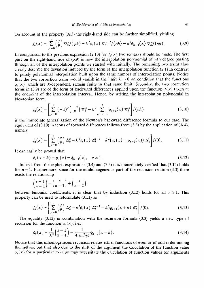
On account of the property (A.3) the right-hand side can be further simplified, yielding

L(x) = ? (;) W(Ph) - k*+,(x) W1f(nh) - k*+,+,(x) CW). (3.9) p=o

In comparison to the previous expression (2.13) for f,(x) two remarks should be made. The first part on the right-hand side of (3.9) is now the interpolation polynomial of nth degree passing through all of the interpolation points we started with initially. The remaining two terms thus clearly describe the deviation induced by the form of the interpolation function (2.1) in contrast to purely polynomial interpolation built upon the same number of interpolation points. Notice that the two correction terms would vanish in the limit k + 0 on condition that the functions C&(X), which are k-dependent, remain finite in that same limit. Secondly, the two correction terms in (3.9) are of the form of backward differences applied upon the function f(x) taken at the endpoint of the interpolation interval. Hence, by writing the interpolation polynomial in Newtonian form,

f,(x) = ? W( p”) [

VR- k2 5 $,+i(x) vhp f(nh) 1

(3.10) p=o p=n-1

is the immediate generalization of the Newton’s backward difference formula to our case. The equivalent of (3.10) in terms of forward differences follows from (3.8) by the application of (A.4) namely

f,(x)= ? (8) [

AR -k*&,(x) A;-’ - k*@+,,(x) + %+,(x>) A?, f(O). 1 (3.11) p=o

It can easily be proved that

&,(x + h) - +?Jx> =%-i(x), n 2 I. (3.12)

Indeed, from the explicit expressions (3.4) and (3.5) it is immediately verified that (3.12) holds for n = 1. Furthermore, since for the nonhomogeneous part of the recursion relation (3.3) there exists the relationship

between binomial coefficients, it is clear that by induction (3.12) holds for all n >, 1. This property can be used to reformulate (3.11) as

A{ - k*&,(x) A$-’ - k2$,+,(x + h) A; f(0). I

(3.13)

The equality (3.12) in combination with the recursion formula (3.3) yields a new type of recursion for the function &n(x), i.e.,

(3.14)

Notice that this inhomogeneous recursion relates either functions of even or of odd order among themselves, but that also due to the shift of the argument the calculation of the function value C&,(X) for a particular x-value may necessitate the calculation of function values for arguments


outside the segment of interpolation. But, of course, the domain of the functions &n(x), n = 1, 2 ,*.., should not be restricted to the segment [0, nh] anyhow. In the following section we shall further investigate the properties of the functions &(x).

4. Further properties of the functions &I,(x)

We introduce the particular function f”(x, n) = xnP1 /(n - l)! depending on the integer parameter n 2 1. From the theory of polynomial interpolation, it is known that the equality

(4-l)

holds for all the functions f(x), x E R, for which the series converges. In particular, we find

A’,f”(O, n), n >, 1, (4.2)

since Aff”(0, n) = 0 for all j 2 n. On the other hand, formula (A.5) of Appendix A teaches us that

= A”-‘_

x=0 (4.3)

Making use of the expression (3.9) for the interpolation function of mixed type, the foregoing results lead to:

which also shows that

E,,(f”(x, n), x) :=f”(x, n) -f;(x, n) = k2h”-‘r&(x). (4.5)

Hence the function c$,,( x) can be interpreted as l/( k2h”-‘) times the error term from mixed type interpolation of order n applied to the particular function f( x, n). This result can be used to check the validity of the expressions (3.5) and (3.6) of the function: &(x) and G2( x), respectively. Indeed, for n = 1 the interpolation function is of the form fl(x, 1) = a cos kx + b sin kx where a and b follow from the conditions f;(O, 1) =A( h, 1) = 1 = f”( x, l), namely a = 1 and b = tan i@. Hence, the error term is given by

E,(f”(x, l), x) = I- cos kx - tan :O sin kx,

from which by means of the relationship (4.5) expression (3.5) is retrieved. A similar calculation permits to confirm (3.6).

From (3.4) we see that &o(x) is an odd function of x, whereas from (3.5) we see that &(x + ih) is an even function of x. These results can be generalized to the following property:

$&nh-x)=(-l)n+l&,($zh+~), n>,O. (4-6)


The proof goes by induction. Assuming that the property holds up to a certain value n - 1, then it follows from (3.14) that

~~-*(:nh + x - h) I

= ( -1)“+1~&z/2 +x).

Let us now define the differential operator

L, = k2D”-’ + D”+i, n > 1. (4.7)

Then any interpolation function f,(x) of order n, as given by (2.1) clearly satisfies the homogeneous differential equation

L?J&) = 0. (4.8)

Hence, f,(x) is the particular solution of the differential equation (4.8) of (n + 1)th order, which satisfies the n + 1 boundary conditions f,( xj) =f( x,), j = 0, 1,. . . , n. From (2.2) it follows that

L,E,,(f, x) = L,f(x) = k*f’“-“(x) +f@+l)(x) (4.9)

and E,( f, x) is the particular solution of the nonhomogeneous differential equation (4.9) which satisfies the n + 1 boundary conditions E,( f, xi) = 0, j = 0, 1,. . . , n. Let us calculate the action of the operator L, upon the function C&,(X). From the explicit form (2.12) of r&(x) and making use of the fact that L, annihilates sin kx and cos kx, we immediately find

However, L,(i) = 0 for all p < n - 1, whereas a direct calculation shows that

=kZ h”-1 ’

It immediately follows that

L,+Jx) = h’-“. (4.10)

64 H. De Meyer et al. / Mixed interpoIation

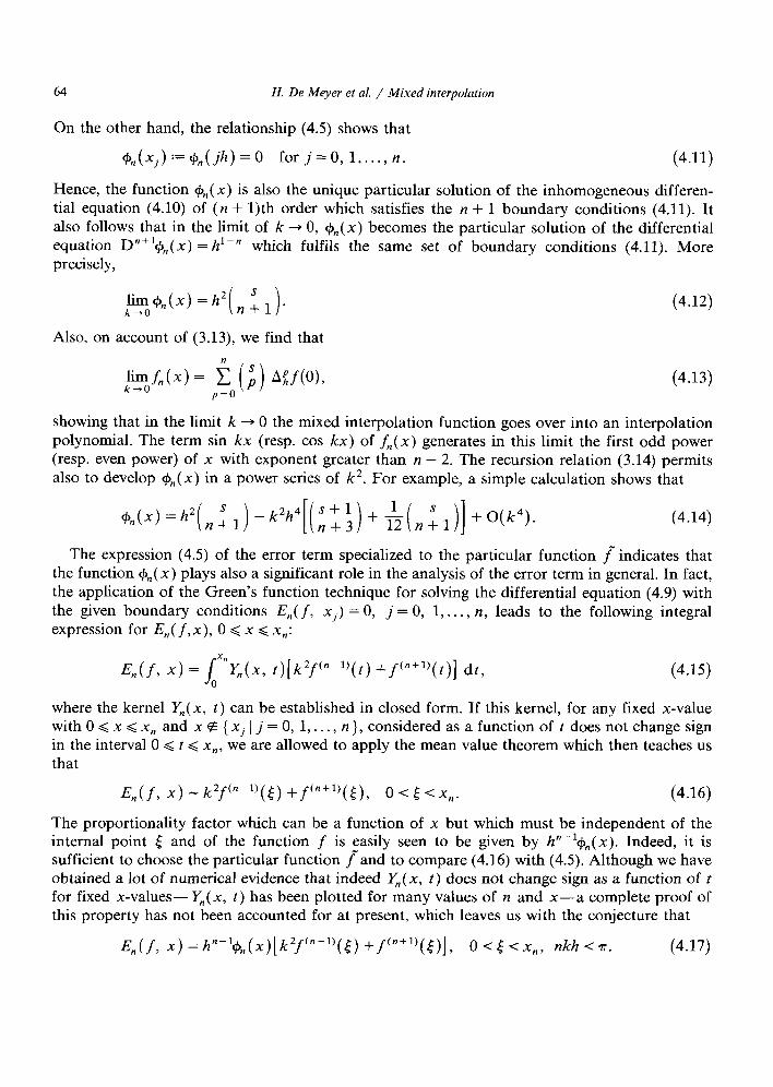
On the other hand, the relationship (4.5) shows that

+n(xi):=+n(jh)=O forj=O,l,..., n. (4.11)

Hence, the function &,(x) is also the unique particular solution of the inhomogeneous differential equation (4.10) of (n + 1)th order which satisfies the n + 1 boundary conditions (4.11). It also follows that in the limit of k + 0, C&(X) becomes the particular solution of the differential equation D”+l$n(x) = h’-” which fulfils the same set of boundary conditions (4.11). More precisely,

(4.12)

Also, on account of (3.13), we find that

(4.13)

showing that in the limit k -+ 0 the mixed interpolation function goes over into an interpolation polynomial. The term sin kx (resp. cos kx) of f,(x) generates in this limit the first odd power (resp. even power) of x with exponent greater than n - 2. The recursion relation (3.14) permits also to develop Gn(x) in a power series of k2. For example, a simple calculation shows that

(4.14)

The expression (4.5) of the error term specialized to the particular function f” indicates that the function C&(X) plays also a significant role in the analysis of the error term in general. In fact, the application of the Green’s function technique for solving the differential equation (4.9) with the given boundary conditions E,( f, xj) = 0, j = 0, 1,. . . , n, leads to the following integral expression for E,( f,x), 0 < x < x,:

E,(f, x) = iX”y,(x, t)[k2f’“-l’(t) +f@+‘)(t)] dt, (4.15)

where the kernel Y,( x, t) can be established in closed form. If this kernel, for any fixed x-value with 0 < x < x, and x @ { xj 1 j = 0, 1,. . . , n }, considered as a function of t does not change sign in the interval 0 < t G x,, we are allowed to apply the mean value theorem which then teaches us that

E,(f, x) -k2f’“-l’(t) +f’“+l’([), O<&cx,,. (4.16)

The proportionality factor which can be a function of x but which must be independent of the internal point 5 and of the function f is easily seen to be given by h”-l+n(x). Indeed, it is sufficient to choose the particular function f-and to compare (4.16) with (4.5). Although we have obtained a lot of numerical evidence that indeed Y,( x, t) does not change sign as a function of t

for fixed x-values-YY,(x, t) has been plotted for many values of n and x-a complete proof of this property has not been accounted for at present, which leaves us with the conjecture that

&(f, x)=h”-‘~$,,(x)[k~f(~-~)(~)+f(“+~)(~)], O<[<x,, nkh<T. (4.17)


5. Conclusion

We have proved that for every function f there exists a unique function f,(x) of the form a cos kx + b sin kx + C~L~cixi which interpolates f(x) at the n + 1 equidistant points jh, j=O ,..*, n. Herein k denotes a real parameter so that kh is no integer multiple of 7~. This mixed type of interpolation is a generalization of polynomial interpolation. The interpolation function f,(x) can be written as a sum of the interpolation polynomial based on the n + 1 points considered and two correction terms - k2+,( x) A’j-‘f(0) - k2&,+1( x + h) A: f(0). The function +,,(x) can be calculated recursively and plays an important role in the discussion of the error term E,( f, x) = f(x) -f,(x). The three functions f,(x), C&(X) and E,( f, x) satisfy each a differential equation with differential operator L, = k2D”-’ + Dn+’ but with different right-hand side: 0, h”-’ and k2f’“-‘j(x) + fen+‘) (x), respectively. Note that all the results reduce to the known results of the polynomial case when k approaches to 0.

The theory developed in this paper forms the base for the derivation of quadrature rules and multistep methods for first- and second-order differential equations. The quadrature rules are generalized Newton-Cotes formulas and the multistep methods are of the type Adams, Milne, Simpson, Stiirmer, etc. Numerical experiments show the efficiency of such methods. We hope to report on this in the near future.

Acknowledgement

We would like to thank the unknown referee for his valuable suggestions.

Appendix A

The rows of the matrix of the linear system (2.3) have the form

[cos 18 sin 10 1 Ih (lh)2 . . . (lh)n~2]~,=,,l ,,,,, nj, (A4

whereby 8 = hk. The determinant A, of this matrix is invariant under the operation of adding to any row componentwise any linear combination of the other rows. Hence, A, is also the determinant of the matrix composed of the consecutive rows

[v,’ cos 10 v,’ sin 18 v,‘(l) vL(lh) vL(lh)’ . . . v~(lh)n~2]~,=,1 ,,, ,,). 3, 1

64.2)

Herein 0,’ := vu represents the backward difference operator of which any power is recursively defined as

v,“+(x) = v,“-‘(v,+(x)) = v,“-‘+(x) - vup-l\c/(.X - U), p E Iv,, (A.31

whereas 0: is the identity operator by convention. Clearly, in (A.2) an expression like 0; cos l/3 is only a short notation for (0; cos x)lxcls. difference AIU := A,,, whereby

In a similar way one can introduce the forward

v:+(x) = A;#(x -pu), p E N. (A4


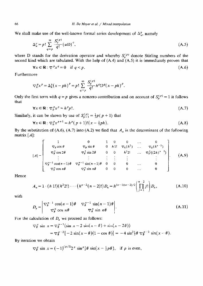
We shall make use of the well-known formal series development of A<, namely

* sJp) Af:=p! c &uDK

4=P

(A-5)

where D stands for the derivation operator and whereby S, (p) denote Stirling numbers of the second kind which are tabulated. With the help of (A.4) and (A.5) it is immediately proven that

VxER: Vpxq=O if q-cp. 64.6)

Furthermore

O” Sip) vhpxp = A;(x -~Iz)~ =p! c qrhqDq(x -ph)P.

4=P .

Only the first term with q =p gives a nonzero contribution and on account of Sjp) = 1 it follows that

VXER: v/xP=hPp!. (A-7)

Similarly, it can be shown by use of Sdf\ = $p( p + 1) that

VxElW: qxp+t== p h (p+l)!(x- :ph). 64.8)

By the substitution of (A.6), (A.7) into (A.2) we find that A,, is the determinant of the following matrix [A]:

1 0 1 0 0 . . . 0

V@COS e ve sin f3 0 hl! v,(h2) . . Vh(h”_2)

V; cos 28 0 0 h22! . . . [Al= :

0; sin 20 v)3(2h>“-*) . . (A.9) . . . .

vt? n-1 cOscn -i)e v,“-’ sin(n -l)f3 0 0 0 . . . 0

0; cos nB 0,” sin n0 0 0 0 ..* 0

Hence

n-2

A, = 1. (h l!)(h*2!) . . . (h"-2(n - 2)!)Q = h("-1)("-2)/2

i 1 JTJ! on3

with

0,~ ve n-1 cos( n - l)f3 v,“-’ sin( n - 1)19

0,” cos n9 v;sinnt? .

For the calculation of D,, we proceed as follows:

vBp sin x = Vi-* (sin x - 2 sin(x - 13) + sin(x - 28))

= vg-* [ - 2 sin( x - e>(i - cos e)] = - 4 sin*+0 vSp-* sin( x - e).

By iteration we obtain

v,P sin x = ( - 1) (p’2)2p sinPi sin(x - +pe), if p is even,

(A.lO)

(A.ll)


and

v,P sin x = (- l)(p-1)‘22p-’ sinP-’ if9 VB sin( x - +( p - 1) 0)

= ( -l)(p-1)‘22P sinP:0 cos(x - +pB), if p is odd.

Putting x = p0 herein and doing similar calculations for Vi cos x we arrive at the following results:

vBp sin pe = i

(- l)p’22p sinPi sin ipe, p even,

(- l)(p-1)‘22p sinPi cos ipe, p odd,

O,” ‘OS “= i

(- l)p’22p sinPi cos +pO, p even,

(_ l)(P+1)/22P sinP+e sin +pe, p odd.

It immediately follows that

D,, = 0,” sin nl3 ~7,“~’ COS(TI - i>e - 0,” cos ne v;-l sin(n - 1)s

= 2 2n-1 sin2”-‘@ cos :e, Vn E IV,,

which in combination with (A.lO) proves (2.4).

Appendix B

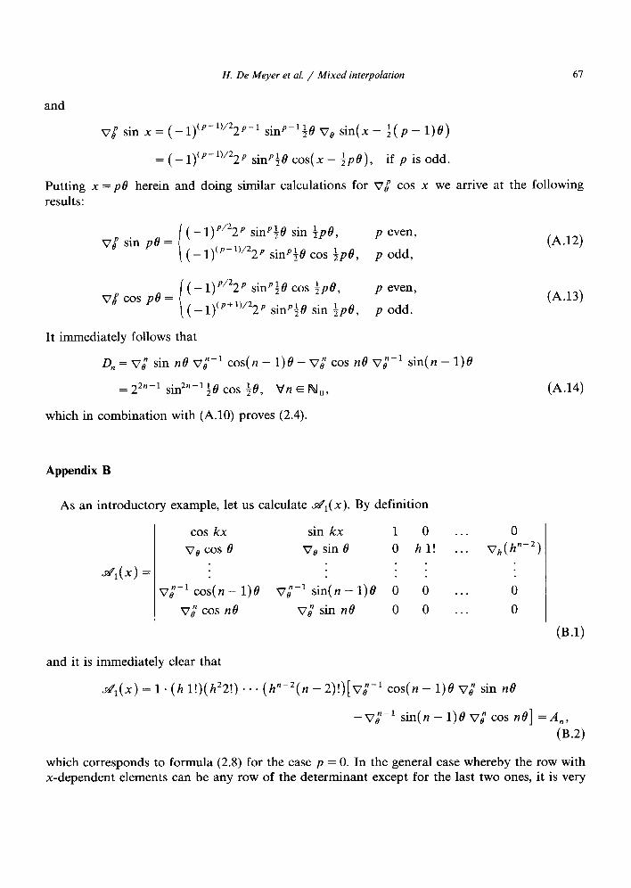
As an introductory example, let us calculate .E@‘~( x). By definition

cos kx sin kx 1 0

V* cog e vO sin e 0 hl!

.zqx)= :

vF9 n-l cOs(n - i)e v;-’ sin(n - 1)0 0 0

0; cos ne 0; sin ne 0 0

and it is immediately clear that

. . . 0

. . . vh( hn-2)

. . . 0

. . . 0

d*(x) = 1. (h l!)(h22!). * * (h”-2(n - 2)!)[v;-l cos(n - 1)e ve” sin ne

(A.12)

(A.13)

(A.14)

(B-1)

-v,“-1 sin(n - i>e 0,” cos ne] =A,,

(W

which corresponds to formula (2.8) for the case p = 0. In the general case whereby the row with x-dependent elements can be any row of the determinant except for the last two ones, it is very

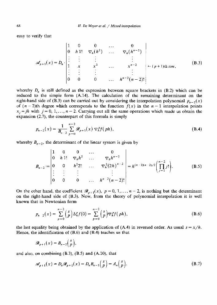
68

easy to verify that

H. De Meyer et al. / Mixed interpolation

~p+lb) = Dn. n-2 (B-3) X + (p + 1)th row,

whereby D, is still defined as the expression between square brackets in (B.2) which can be reduced to the simple form (A.14). The calculation of the remaining determinant on the right-hand side of (B.3) can be carried out by considering the interpolation polynomial P~_~(x) of (n - 2)th degree which corresponds to the function f(x) in the n - 1 interpolation points xi =jh with j = 0, 1,. . . , n - 2. Carrying out all the same operations which made us obtain the expansion (2.7), the counterpart of this formula is simply

Pn-2(X) = + n-2

c 9p+dX) a=ea p=o

* n-2

(B.4)

whereby Bn_2, the determinant of the linear system is given by

B,,_2 :=

1 0 0 . . . 0

0 h l! vhh2 . . . v,,hn-2

0 0 h22! ._. v;(2h)“-2

0 0 0 . . . h”-2(; - 2)!

= h(“-l)(“-2)/z (B.5)

On the other hand, the coefficient ap+t( x), p = 0, 1,. . . , n - 2, is nothing but the determinant on the right-hand side of (B.3). Now, from the theory of polynomial interpolation it is well known that in Newtonian form

~n-2(4= n~2(;)W(o)= n~2(;)Gf(ph), p=o p=o

the last equality being obtained by the application of (A.4) Hence, the identification of (B.6) and (B.4) teaches us that

ap+1(4 = Bn- ( 1 ;rT and also, on combining (B.3), (B.5) and (A.lO), that

tw

in reversed order. As usual s = x/h.

(B.7)


Note added in proof

The validity of (4.16) and a rigorous study of the error term are subject of a separate paper (H. De Meyer, J. Vanthournout, G. Vanden Berghe and A. Vanderbauwhede, On the error estima- tion for a mixed type of interpolation). In this paper we have proved that (4.17) holds.

References

[l] D.G. Bettis, Numerical integration of products of Fourier and ordinary polynomials, Numer. Math. 14 (1970) 421-434.

[2] P.J. Davis and P. Rabinowitz, Methods of Numerical Integration (Academic Press, New York, 1984). [3] U.T. Ehrenmark, A three-point formula for numerical quadrature of oscillatory integrals with variable frequency,

J. Comput. Appl. Math. 21 (1) (1988) 87-99. [4] L.N.G. Filon, On a quadrature formula for trigonometric integrals, Proc. Roy. Sot. Edinburgh 49 (1928) 38-47. [5] E.A. Flinn, A modification of Filon’s method of numerical integration, J. Assoc. Comput. Mach. 7 (1960)

181-184.

[b] W. Gautschi, Numerical integration of ordinary differential equations based on trigonometric polynomials, Numer. Math. 3 (1961) 381-397.

[7] D. Levin, Procedure for computing one- and two-dimensional integrals of functions with rapid irregular oscillations, Math. Camp. 38 (1982) 531-538.

[8] Y.L. Luke, On the computation of oscillatory integrals, Proc. Cambridge Phil. Sot. 50 (1954) 269-277. [9] T. Lyche, Chebyshevian multistep methods for ordinary differental equations, Numer. Math. 19 (1972) 65-75.

[lo] B. Neta, Families of backward differentation methods based on trigonometric polynomials, J. Comput. Math. 20 (1986) 67-75.

[ll] B. Neta and C.H. Ford, Families of methods for ordinary differential equations based on trigonometric polynomials, .I. Comput. Appl. Math. 10 (1) (1984) 33-38.

[12] A. Raptis and A.C. Allison, Exponential-fitting methods for the numerical solution of the Schrijdinger equation, Comput. Phys. Comm. 4 (1978) l-5.

[13] E. Stiefel and D.G. Bettis, Stabilization of Cowell’s method, Numer. Math. 13 (1969) 154-175. [14] E.O. Tuck, A simple ‘Filon-trapezoidal’ rule, Math. Comp. 21 (1967) 239-241. [15] P.J. van der Houwen and B.P. Sommeijer, Linear multistep methods with reduced truncation error for periodic

initial value problems, ZMA J. Numer. Anal. 4 (1984) 479-489.

on a new type of mixed interpolation - core.ac.uk h. de meyer et al. / mixed interpolation by...

Documents