on a new approach to cointegration { the state …euclid.ucc.ie/hanzon/budapest2007.pdfon a new...
TRANSCRIPT

On a New Approach to Cointegration – The State-Space ErrorCorrection Model
Thomas Ribarits† and Bernard Hanzon‡
† European Investment BankRisk Management DirectorateFinancial Risk Department
100, boulevard Konrad Adenauer, L-2950 Luxembourg
E-mail: [email protected]‡ University College Cork
School of Mathematical SciencesCork, Ireland
E-mail: [email protected]
Summary In this paper we consider cointegrated I(1) processes in the state-space framework. We intro-duce the state-space error correction model (SSECM) and provide a complete treatment of how to estimateSSECMs by (pseudo-)maximum likelihood methods, including reduced rank regression techniques. In doingso, we follow very closely the Johansen approach for the VAR case; see Johansen (1995). The remainingfree parameters will be represented using a novel type of local parametrization. Simulation studies and areal world application clearly reveal the potential of the new approach.
Keywords: Cointegration, state-space models, data-driven local coordinates, maximum likelihood estima-tion, reduced rank regression.
1. INTRODUCTION
The main aim of this paper lies in the generalization of the classical cointegration analysis of Johansen(1995) from the VAR framework to the state-space case. The motivations for this effort are the following:
• State-space models offer a larger and more flexible model class, containing VAR models as specialcases.• State-space and VARMA models are equivalent, yet the state-space approach offers many practical
advantages such as simpler parametrization and more efficient methods to compute likelihood functionsand their gradients.• In practice, the data generating process (DGP) will typically neither be of VAR nor of VARMA type.
Yet, its approximation by means of a state-space model will in general require less parameters thanby means of a VAR model.• State-space models are heavily used in continuous-time modelling, especially in financial applications,
and discrete-time versions of such continuous-time state-space models are most naturally presentedas discrete-time state-space models; examples include the work of Dai and Singleton (2000) on affineterm structure models and references mentioned there.
In our attempt to generalize VAR cointegration to cointegration analysis in the state-space framework wewill proceed along the lines of classical VAR cointegration. In Johansen’s celebrated method for calculatingThis paper has been presented at the 62nd European Meeting of the Econometric Society, 27 – 31 August 2007, Budapest,Hungary.

2 Thomas Ribarits and Bernard Hanzon
the maximum likelihood estimator of a cointegrated VAR model, the mathematical core can be summarizedas follows:
1 First, a reduction of the likelihood maximization problem to a so-called reduced rank regression prob-lem is achieved by ‘concentrating out’ a number of linear parameters in the VAR representation.
2 Then, the reduced-rank regression problem is solved.3 After this concentration step, one is left with the problem of finding the optimum of a quotient of
determinants of matrices which are quadratic in terms of an unknown matrix, β say; this unknownmatrix β needs to be determined in such a way that an optimum is reached. The optimum can becalculated based on the solution of a generalized eigenvalue-eigenvector problem.
4 Steps 1–3 above solve the maximum likelihood problem in the VAR case, no other parameters remainto be estimated.
In the present paper this methodology is generalized to the case of cointegrated linear state-space models.To this end, we will first – in analogy to the celebrated VECM, the (autoregressive) vector error correctionmodel – introduce the state-space error correction model which will be abbreviated by SSECM.
Then, mimicking the estimation of autoregressive VAR error correction models, the number of parametersappearing in the original non-linear likelihood optimization problem will be reduced by sequentially ‘con-centrating out’ parameters with respect to which the optimization problem can be solved analytically.More precisely, the idea is that
1 by fixing two of the three matrices in the state-space representation, the constrained likelihood max-imization problem can be reduced to a reduced rank regression problem by ‘concentrating out’ thethird state-space matrix.
2 Then, the reduced-rank regression problem is solved.3 After this concentration step, one is left with a problem of finding the optimum of a quotient of
determinants of matrices being quadratic in terms of an unknown matrix β which is similar to step(3.) in the VAR case above. In general, the optimum can now be calculated based on the solution ofa reduced rank generalized eigenvalue-eigenvector problem.
4 In contrast to the VAR case, substituting the optimal parameter values obtained in steps 1–3 aboveinto the likelihood function leaves us with a criterion function that still depends on some (but a muchsmaller number of) unknown parameters. Instead of trying to choose a particular canonical form forthe two matrices in the state-space representation that remain to be determined, we apply the so-calledDDLC approach, a simple local parametrization technique which has been used e.g. in McKelveyet al. (2004) and Ribarits et al. (2004) in the context of stationary time series models.
An important remark is that the calculation of the gradient of the concentrated likelihood function, in caseit exists, can be done by calculating the gradient of the original likelihood function before ‘concentration’at the parameter point that results from the concentration step. Moreover, even if the concentrated likeli-hood function shall turn out to be non-differentiable, the ‘adapted’ gradient-based search algorithmproposed in this paper, which operates only on the remaining free parameters (after ‘concentration’), is stillensured not to get stuck at any other point than a critical point of the original likelihood function!1 Hence,
1The importance of this lies in the fact that differentiation of eigenvalues and eigenvectors, which could lead to very tediousdifferentiation calculations in the algorithm, can be avoided in this way and very efficient numerical differentiation techniquescan be directly applied to the original likelihood function. It is also important from the mathematical view-point as eigenvaluesand eigenvectors obtained in the last concentration step need not be differentiable, potentially leading to a non-differentiableconcentrated likelihood function.
62nd European Meeting of the Econometric Society, 27 – 31 August 2007, Budapest

On a New Approach to Cointegration – The State-Space Error Correction Model 3
one can find a local optimum of the likelihood function by means of a gradient-type search method, like forinstance the Gauss-Newton algorithm. This in turn implies, at least for suffciently large number of data,that we find the maximum likelihood estimator.
Using either
• Johansen’s classical VAR approach – the cointegrated VAR model obtained can be written in state-space form, and the state dimension can easily be reduced by a ‘truncating approach’• or so-called (regression based) subspace algorithms
the determination of integer-valued parameters (the system order and the number of common trends) isperformed. Both approaches also provide the user with good starting values for the remaining unknownreal-valued parameters in the likelihood optimization problem.
The paper is organized as follows: In Section 2 the concept of cointegrated processes of order one is brieflyreviewed. Section 3 introduces state-space models for cointegrated processes and, most importantly, thenew state-space error correction model SSECM. Section 4 gives details on how we propose to approachthe estimation problem for SSECMs by means of (pseudo-)maximum likelihood methods. Here, a stepwise‘concentration’ of the likelihood is performed, leading to a generalized eigenvalue problem in the finalstep. In Section 5 we apply a new parametrization method (DDLC) in order to further reduce the number ofparameters in the non-linear likelihood optimization problem. Section 6 intends to give a very brief overviewof how model selection can be performed in the framework of SSECMs and also treats the question of howto obtain initial estimates for the real-valued parameters. In Section 7 we apply the new approach in twoways: First, a simulation study is performed using the data generating processes presented in Saikkonen andLuukkonen (1997). Second, data of the US economy as presented in Lutkepohl (1991) and Lutkepohl andClaessen (1997) are used in order to demonstrate the practicability of the proposed procedure. We finish inSection 8 with a summary and concluding remarks.
2. MOTIVATION FOR COINTEGRATION
Econometric time series often show non-stationarities, e.g. trends in the mean and variance. Whereas eachindividual component of the time series might show such non-stationary behaviour, econonomic theory maysuggest that there are static long-term equilibrium relations between the variables under consideration. Suchequilibrium relations, which are lost by differencing the series but contain important economic information,will in general not be satisfied exactly at each point in time. The idea, however, is that the deviation fromthe equilibrium relation at each point in time is at least ‘small’, namely stationary, as compared to the‘large’, namely non-stationary, individual variables.
One way of modeling non-stationarities is by making use of integrated processes: A p-dimensional process(yt|t ∈ N) is called integrated of order 1, or briefly I(1), if ∆yt = (1− z)yt is ‘stationary’, where z denotesthe Lag operator, i.e. z(yt|t ∈ N) = (0, y1, y2, . . . ).
In order to model the equilibrium relations, one usually resorts to cointegrated processes: An integratedvector valued process is called cointegrated if there exists at least one vector 0 6= β ∈ Rp such that the process(β′yt)t∈N is ‘stationary’. As is well known, the number of such linear independent cointegrating vectors β iscalled the rank of cointegration, r say. The number c = s− r is the number of common trends. The subspaceof Rp spanned by the cointegrating vectors is called the cointegrating space.
As mentioned above, the equilibrium relations are not ‘exact’. However, the stationary deviation from
62nd European Meeting of the Econometric Society, 27 – 31 August 2007, Budapest

4 Thomas Ribarits and Bernard Hanzon
an exact equilibrium relation, given by (β′yt) − 0, is relatively ‘small’ compared to the non-stationarycomponents of (yt).
Figure 2 shows an example of a bivariate cointegrated process.
Zeit
0 50 100 150 200 250 300
010
2030
4050
60
Y[t]: Income C[t]: Consumption 0.7 Y[t] − C[t] = stationary
Figure 1. A cointegrated process (Yt, Ct)′ with a cointegrating relation β = (0.7,−1)′; β ∈ R2 is determinedup to a multiplicative constant (unequal zero).
3. THE STATE-SPACE ERROR CORRECTION MODEL
We start by briefly discussing state-space representations of I(1) processes. Consider the following linear,time invariant, discrete-time state-space system:
xt+1 = Axt +Bεt, x1 = 0 (3.1)yt = Cxt + εt (3.2)
Here, xt is the n-dimensional state vector, which is, in general, unobserved; A ∈ Rn×n, B ∈ Rn×p andC ∈ Rp×n are parameter matrices; yt is the observed p-dimensional output. In addition, (εt)t∈N is a p-dimensional (weak) white noise process with Eεt = 0 and Eεtε′t = Σ.
The state-space system in (3.1, 3.2) is called minimal if rk[B,AB, . . . , An−1B
]=rk
[C ′, A′C ′, . . . , (A′)n−1C ′
]′ =n. It is called stable if the stability condition |λmax(A)| < 1 is satisfied, where λmax(A) denotes an eigenvalueof A of maximum modulus.
It can be shown that for (yt) to be I(1), A must have an eigenvalue of one: λi(A) = 1 must hold for somei ∈ {1, . . . , n}. Moreover, the algebraic multiplicity of the eigenvalue one must coincide with its geometricmultiplicity, c say; see Bauer and Wagner (2003). If this is not the case, (yt) will show higher ordersof integration. As mentioned in Section 2 above, the number c is the number of common trends. Whenreferring to the state-space model (3.1,3.2) in the sequel, we will always assume A to have an eigenvalueone of (algebraic and geometric) multiplicity c.
Note that setting up a state-space model (3.1,3.2) for some observed I(1) process (yt) requires the estimation
62nd European Meeting of the Econometric Society, 27 – 31 August 2007, Budapest
On a New Approach to Cointegration – The State-Space Error Correction Model 5
of both integer-valued parameters n and c and real-value parameters in ((A,B,C),Σ). As we shall see below,there is an inherent problem of non-identifiability for the latter parameters.
A solution to (3.1,3.2) can be given by yt =∑∞j=1 CA
j−1Bεt−j + εt where we put εt = 0 for t ≤ 0. Using ashorthand notation, such solution can be written as
yt = k(z)εt (3.3)= [Cz(I − zA)−1B + I]εt
= [∞∑j=1
CAj−1Bzj + I]εt
Here, z ∈ C is interpreted as a complex variable, and k(z) is called the transfer function corresponding to thestate-space model. The transfer function is a rational matrix-valued function and describes the input-outputbehavior of the state-space system, with (εt) being viewed as input and (yt) as output.
For writing down the Gaussian likelihood function, we will make use of the one step prediction errorsεt = yt − E(yt|y1, . . . yt−1). The latter can be obtained by simply rewriting equations (3.1,3.2):
xt+1 =
A︷ ︸︸ ︷(A−BC)xt +
B︷︸︸︷B yt (3.4)
εt(A, B, C) = −C︸︷︷︸C
xt + yt (3.5)
Note that (3.4,3.5) represents the inverse state-space system, i.e. the system with inputs (yt) and outputs(εt). The transfer function corresponding to the inverse system is given by
εt = k(z)yt (3.6)= [Cz(I − zA)−1B + I]yt
= [∞∑j=1
CAj−1Bzj + I]yt
Recall that A has an eigenvalue one of multiplicity c, and this implies that the inverse transfer function k(z)has a c-fold root at one, i.e. k(1) ∈ Rp×p has rank p− c only! We can thus write
k(1) = C(I − A)−1B + I = −αβ′ α ∈ Rp×r, β ∈ Rp×r (3.7)
where r = p − c. Equation (3.7) is in fact the starting point for deriving the state-space error correctionmodel SSECM. Note that we have
k(z) = k(1)z +
= 0 at z = 1= I at z = 0︷ ︸︸ ︷[k(z)− k(1)z
]= k(1)z + (1− z)
[I − k(z)
]= k(1)z + I(1− z)− k(z)(1− z) (3.8)
where k(0) = 0 must hold true. Putting k(z) =∑∞j=0 Kjz
j , we therefore get K0 = 0. The other Kj areeasily obtained by means of a comparison of coefficients:
Kj =∞∑
i=j+1
Ki =
C︷ ︸︸ ︷[CA(I − A)−1
] Aj−1︷ ︸︸ ︷Aj−1
B︷︸︸︷B , j ≥ 1 (3.9)
62nd European Meeting of the Econometric Society, 27 – 31 August 2007, Budapest
6 Thomas Ribarits and Bernard Hanzon
Substituting (3.8) and (3.7) into εt = k(z)yt, we obtain
εt = k(z)yt (3.10)= −αβ′yt−1 + ∆yt − k(z)∆yt
Using (3.9), k(z)∆yt can be represented in state-space form as follows:
xt+1 = Axt + B∆yt (3.11)k(z)∆yt = CA(I − A)−1xt
We are now ready to formulate the state-space error correction model (SSECM):
∆yt = αβ′yt−1 + CA(I − A)−1xt + εtwhere αβ′ = −
[C(I − A)−1B + Ip
]xt+1 = Axt + B∆yt
(3.12)
4. MAXIMUM LIKELIHOOD ESTIMATION OF SSECMS
We will assume that n > p and rank(B) = p in the sequel. This is mainly done for pedagogical reasons as theother cases require purely technical adjustments which do not provide any value added for the clarification ofthe applied principles. For a unified treatment of all possible cases as well as proofs of the results presentedbelow, the reader is referred to Ribarits and Hanzon (2005).
In analogy to the VAR-case in Johansen (1995), we set
Z0t = ∆yt, Z1t = yt−1, Z2t = xt, Mij =1T
T∑t=1
ZitZ′jt
Finding the (Gaussian) maximum likelihood estimator for the parameters in (3.12) translates to solving thefollowing non-linear constrained optimization problem:
minL(α, β, A, B, C,Σ) = log det Σ +1
T
T∑t=1
(Z0t − αβ′Z1t − CA(I − A)−1Z2t)′Σ−1(Z0t − αβ′Z1t − CA(I − A)−1Z2t)
s. t. C[(I − A)−1B] = −(Ip + αβ′) (4.13)
This problem is tackled by performing a series of ‘concentration steps’.
4.1. Step 1: Concentrating out C
Let (α, β, A, B,Σ) be given and assume that M22 > 0. Then the unique global constrained minimizer solvingminC L(α, β, A, B, C,Σ) is independent of Σ and is given by
ˆC = [M02(I − A)−1′A′ − αβ′M12(I − A)−1′A′]H11 − (Ip + αβ′)H21 (4.14)
where(H11 H12
H21 H22
)=(A(I − A)−1M22(I − A)−1′A′ (I − A)−1B
((I − A)−1B)′ 0
)−1
(4.15)
62nd European Meeting of the Econometric Society, 27 – 31 August 2007, Budapest

On a New Approach to Cointegration – The State-Space Error Correction Model 7
Inserting this optimizer into the likelihood function in (4.13) yields
L1c(α, β, A, B,Σ) = L(α, β, A, B, ˆC,Σ)
= log det Σ +1T
T∑t=1
(R0t − αβ′R1t)′Σ−1(R0t − αβ′R1t) (4.16)
where R0t = Z0t −(
[M02(I − A)−1′A′]H11 −H21
)A(I − A)−1Z2t (4.17)
R1t = Z1t −(
[M12(I − A)−1′A′]H11 +H21
)A(I − A)−1Z2t (4.18)
4.2. Step 2: Concentrating out α
Let us denote by Sij the (non-centered) sample covariance matrices of the residuals Ri and Rj , i.e.
Sij =1T
T∑t=1
RitR′jt
Furtermore, let (β, A, B,Σ) be given such that β′S11β > 0. We note that this restriction is ‘innocent’ asit will typically hold true; see Section ‘Concentrating out α1’ in Ribarits and Hanzon (2005) for a detaileddiscussion, showing in fact that S11 > 0 can be assumed in the case considered in this paper. The uniqueglobal minimizer solving minα L1c(α, β, A, B,Σ) is independent of Σ and is given by
α = S01β(β′S11β)−1 (4.19)
Inserting this optimizer into the likelihood function in (4.16) yields
L2c(β, A, B,Σ) = L1c(α, β, A, B,Σ) = (4.20)
log det Σ +1T
T∑t=1
(R0t − S01β(β′S11β)−1β′R1t)′Σ−1(R0t − S01β(β′S11β)−1β′R1t)
4.3. Step 3: Concentrating out Σ
This step is very common: Let (β, A, B) be given such that
1T
T∑t=1
(R0t − S01β(β′S11β)−1β′R1t)(R0t − S01β(β′S11β)−1β′R1t)′ > 0
Then the unique global minimizer solving minΣ=Σ′>0 L2c(β, A, B,Σ) is given by
Σ = S00 − S01β(β′S11β)−1β′S10 (4.21)
Inserting (4.21) into (4.20) yields
L3c(β, A, B) = L2c(β, A, B, Σ) = log det[S00 − S01β(β′S11β)−1β′S10
]+ p (4.22)
62nd European Meeting of the Econometric Society, 27 – 31 August 2007, Budapest

8 Thomas Ribarits and Bernard Hanzon
4.4. Step 4: Concentrating out β
As in the VAR case, the minimization of (4.22) with respect to β leads to a generalized eigenvalue problem:Using the equalities
det
(Σ11 Σ12Σ21 Σ22
)= det Σ11 · det
[Σ22 − Σ21Σ
−111 Σ12
]= det Σ22 · det
[Σ11 − Σ12Σ
−122 Σ21
]⇒
det
(S00 S01ββ′S10 β′S11β
)= detS00 · det
[β′S11β − β′S10S
−100 S01β
]= det β
′S11β · det
[S00 − S01β(β
′S11β)
−1β′S10
]and assuming that S11 > 0, β′S11β > 0 (see Section 4.2 above) and S00 > 0, representing ‘innocent’restrictions, one can rewrite 4.22 as
L3c(β, A, B) = log detS00 + logdetβ′(S11 − S10S
−100 S01)β
detβ′S11β+ p (4.23)
The following lemma treating the generalized eigenvalue problem is recalled for the sake of completeness:
Lemma 4.1. Let M = M ′, N = N ′, M ≥ 0 and N > 0. Then det(λN −M) = 0 has p solutions λ1 ≥· · · ≥ λp ≥ 0 with eigenvectors V = [v1, . . . , vp] such that MV = NV Λ, V ′NV = I and V ′MV = Λ, whereΛ = diag(λ1, . . . , λp).
Putting M = S10S−100 S01 and N = S11, all global minimizers solving minβ L3c(β, A, B) in (4.23) are then
easily seen to be given byβ = [v1, . . . , vr] · T , T ∈ Gl(r) (4.24)
where T ∈ GL(r) is arbitrary and v1, . . . , vr are the eigenvectors corresponding to the r largest eigenvaluesλ1, . . . , λr of the generalized eigenvalue problem det(λS11 − S10S
−100 S01) = 0. Note that we assume λ1 ≥
· · · ≥ λr > λr+1 ≥ · · · > λs > 0. We remark that in general, e.g. if n < p, this ‘concentration step’ becomesa reduced rank generalized eigenvalue problem; see Section ‘Concentrating out β1’ in Ribarits and Hanzon(2005).
Inserting the optimizing arguments into (4.23) finally yields
L4c(A, B) = L3c(β, A, B) = log detS00 + log Πri=1(1− λi) + p (4.25)
We have thus reduced the original likelihood optimization problem in (α, β, A, B, C,Σ) to a problem in(A, B) only. The following section treats the question of whether a further reduction of the number ofparameters is still possible.
5. PARAMETRIZATION OF (A, B) USING THE DDLC APPROACH
The parameters in (A, B) are non-identifiable: Let Gl(n) denote the set of real non-singular n×n matrices.It is not difficult to see that (A, B) and (TAT−1, T B), T ∈ Gl(n) give rise to (after carrying out in reverseorder the optimization steps described in the sub-sections above) the same original transfer function k(z)and therefore the same likelihood value.
In order to treat the problem of the non-identifiability in (A, B), we introduce a novel local parametrization,making use of the so-called DDLC philosophy; see e.g. McKelvey et al. (2004) or Ribarits et al. (2004). DDLCstands for ‘data-driven local coordinates’: The parametrization is of local nature only, i.e. desirable propertiesfor a parametrization can only be shown in an open neighborhood of a given point in the parameter space.Moreover, the parametrization can be viewed as a collection of (uncountably many) coordinate charts, where
62nd European Meeting of the Econometric Society, 27 – 31 August 2007, Budapest

On a New Approach to Cointegration – The State-Space Error Correction Model 9
the choice between these charts can be made in a data-driven manner. As will be seen below, we will changechart in each step of the iterative search algorithm.
The idea behind DDLC is simple: The set E(A, B) = {(TAT−1, T B), T ∈ Gl(n)} is called the (A, B)-equivalence class as all its elements (TAT−1, T B) represent the same transfer function and thus the samelikelihood value. This set has the structure of a real analytic submanifold of Rn2+np of dimension n2. Thetangent space, Q(A, B) say, can be easily computed. In fact, (A, B) + (As, Bs) ∈ Q(A, B) ⇔ (As, Bs) =(T A− AT , T B) for some T ∈ Rn×n. Using the relation vec(ABC) = (C ′ ⊗A) vec(B), vectorization yields
Q(A, B) = {(
vec(A)vec(B)
)+(A′ ⊗ In − In ⊗ A
B′ ⊗ In
)︸ ︷︷ ︸
Q∈R(n2+np)×n2
· vec(T ), T ∈ Rn×n} (5.26)
For DDLC, the idea is to consider as a parameter space the np-dimensional ortho-complement, Q⊥ say, tothe tangent space (5.26) at the given (A, B). In this manner, we do not parametrize directions along (thetangent space to) the equivalence class (where the likelihood value stays constant), but we parametrize onlydirections in which the likelihood value changes:
ϕ : Rnp → Rn2+np (5.27)
τ 7→(
vec(A(τ))vec(B(τ))
)=(
vec(A)vec(B)
)+Q⊥τ
Figure 5 illustrates again the main idea of parametrizing only directions in which the likelihood value changes(in first order).
Figure 2. The DDLC philosophy: The thick curve represents the equivalence class E(A, B). Each point inE(A, B) gives rise to the same likelihood value. The (red) dashed straight line represents the tangent spaceQ(A, B). The straight line orthogonal to the dashed one thus corresponds to Q⊥, the ortho-complement ofthe tangent space to the equivalence class, which is the DDLC parameter space.
In the course of an iterative search algorithm, the DDLC construction is iterated in the sense that the pair(A(τ), B(τ)) corresponding to the updated parameter vector τ becomes the new initial (A, B) pair (5.27) in
62nd European Meeting of the Econometric Society, 27 – 31 August 2007, Budapest
10 Thomas Ribarits and Bernard Hanzon
the next step of the iterative search procedure. For details regarding geometrical and topological propertiesof DDLC as well as its numerical advantages see Ribarits et al. (2004), Ribarits et al. (2005) or Ribarits et al.(2004).
Note that for the rest of this paper, τ ∈ Rnp shall denote the DDLC parameter vector in (5.27). Hence, theconcentrated likelihood function (4.25) can finally be rewritten as
L4c(τ) = L4c(A(τ), B(τ)) = log detS00 + log Πri=1(1− λi) + p (5.28)
The remaining problem is to minimize (5.28) with respect to τ . For this purpose, we suggest to employ thefollowing ‘adapted’ gradient-based search algorithm:
• First, compute the gradient of the original likelihood function L(α, β, A, B, C,Σ) in (4.13) with respectto (A, B).• Second, evaluate it at the parameter point that results from the concentration steps, i.e. at the point
(α, β, A, B, C,Σ) = (α, β, A, B, ˆC, Σ), where ˆC, α, Σ and β are given in (4.14), (4.19), (4.21) and(4.24), respectively. This yields, after accounting for the derivative of (A, B) with respect to τ – see(5.27) – the ‘gradient’ of L4c(τ).• In fact, if L4c(τ) is differentiable, such ‘gradient’ represents the genuine gradient of L4c(τ), as is
easily seen from an application of the chain rule. However, even if L4c(τ) shall turn out to be non-differentiable2, it can be shown that along this ‘gradient’ direction the original likelihood function(after carrying out in reverse order the optimization steps) is ensured to decrease if the step size ischosen small enough and a critical point of the original likelihood function has not yet been found.In other words, such ‘adapted’ gradient algorithm can only get stuck at points which coincide withcritical points of the original likelihood function!
Of course, one can in practice also choose a Gauss-Newton type search direction instead of the ‘gradient’direction, in particular as L4c(τ) will typically be differentiable and Gauss-Newton type algorithms do thenusually have better convergence properties.
Apart from the theoretical assurance to decrease the criterion value by employing the ‘adapted’ gradientalgorithm, there is a second, perhaps more apparent, advantage: Differentiating L4c(τ), if possible, wouldamount to a multiple application of the chain rule and to differentiation of eigenvalues and eigenvectorsappearing in one of the concentration steps, which in turn would lead to very tedious calculations in thealgorithm. Instead, the gradient of the original likelihood function L(α, β, A, B, C,Σ) with respect to (A, B)can be computed in a numerically efficient way using so-called extended prediction error filters, and we canavoid computationally expensive and inaccurate numerical differencing methods.
6. MODEL SELECTION AND INITIAL PARAMETER ESTIMATES FOR SSECMS
Note that up to now we have assumed to know both the state dimension n, i.e. the size of the A matrix in(3.12) and the number of common trends c. In practice, these integer-valued parameters have to be estimatedfrom data. Similarly, it is desirable to start the likelihood optimization procedure with some ‘educated guess’for (A, B).
2Note that from the mathematical view-point eigenvalues and eigenvectors, which appear in the final concentration step, neednot be differentiable, and such non-differentiability can translate into non-differentiability of the final concentrated likelihoodfunction L4c(τ)!
62nd European Meeting of the Econometric Society, 27 – 31 August 2007, Budapest

On a New Approach to Cointegration – The State-Space Error Correction Model 11
In principle, one can think of many ways of how to find estimates for n, c and, thereafter, initial estimatesfor (A, B). In the simulation study presented below, we made use of so-called subspace algorithms, whereasin the application to US macroeconomic data we used Johansen’s VAR error correction models. For the sakeof completeness both approaches are briefly sketched in the sequel although the determination of estimatesfor n, c and initial estimates for (A, B) does not fall into the main scope of this paper.
6.1. Model selection based on subspace algorithms
For the estimation of n, we first regress {yt, . . . , yt+f} onto {yt−1, . . . , yt−p}, where we may choose e.g. f =
p = 2kAIC . Here, kAIC denotes the estimated lag order of a VAR model of the form yt =∑kj=1A(j)yt−j+εt,
using the well-known AIC criterion function. Regressing {yt, . . . , yt+f} onto {yt−1, . . . , yt−p} yields a regres-sion matrix, and we consider the number of singular values of the regression matrix that differ significantlyfrom zero as the estimated order, n say. This is done via minimization of an information-type criterion calledSV C(n); see Bauer and Wagner (2002), where this procedure is shown to deliver consistent order estimates.
As far as the estimation of the number of common trends c = p− r is concerned, Bauer and Wagner (2002)provide a possible test sequence, too. The tests are based on the result that under the null hypothesis of ccommon trends (n correctly specified) the asymptotic distribution of the c largest eigenvalues of T (A− In)
is equal to the distribution of the eigenvalues of∫ 1
0W (t)dW ′(t)
[∫ 1
0W (t)W (t)′dt
]−1
, where W (t) is a c-
dimensional standard Brownian motion and A is the estimated A-matrix from the subspace algorithm weuse. A simulation of the distribution can thus be used for the construction of tests to determine c.
Once n and c have been estimated, an initial estimate ( ˆA, ˆB) is obtained by employing the CCA subspacealgorithm. Subspace algorithms, which originate from the systems and control literature, are computationallyunproblematic as they only rely upon linear regressions and a singular value decomposition. For a detailedanalysis of the CCA algorithm in the I(1) context, see Bauer and Wagner (2002).
6.2. Model selection based on Johansen’s VAR approach
An alternative way of determining n, c and an initial estimate for (A, B) follows along the lines of theclassical Johansen approach to cointegration. This route has been taken for the second example presentedin Section 7 below.
First, we estimated a conventional VAR model (in levels). Let kBIC denote the estimated lag order of suchVAR model of the form yt =
∑kj=1A(j)yt−j + εt, using the well-known BIC criterion function.
Given the lag order kBIC , we then performed the classical trace test in Johansen’s VAR error correctionmodel to determine r and thus c = p−r. The resulting VAR error correction model is readily obtained as well,and one can then transform it back to a conventional VAR model which can, in turn, be straightforwardlywritten in state-space form, (Ajoh, Bjoh, Cjoh) say. Note that the state-space representation of a VAR modelis widely known as the ‘companion form of the VAR model’. By construction, the Ajoh matrix has one asc-fold eigenvalue.
Applying a suitable state transformation of the form (Ajoh, Bjoh, Cjoh) = (TAjohT−1, TBjoh, CjohT−1)
62nd European Meeting of the Econometric Society, 27 – 31 August 2007, Budapest
12 Thomas Ribarits and Bernard Hanzon
yields a state-space system with block diagonal Ajoh matrix, i.e.
(xt+1,1
xt+1,2
)=
Ajoh︷ ︸︸ ︷(Ic 00 Astjoh
)(xt,1xt,2
)+
Bjoh︷ ︸︸ ︷(B1joh
Bstjoh
)εt (6.29)
yt =(C1joh, C
stjoh
)︸ ︷︷ ︸
Cjoh
(xt,1xt,2
)+ εt (6.30)
where (Astjoh, Bstjoh, C
stjoh) represents a stable system, i.e. |λmax(Astjoh)| < 1.
In order to detemine n, one can now apply a so-called ‘balance and truncate’ approach to the stablesubsystem. Balanced model truncation is a simple and, nevertheless, efficient model reduction technique forstate-space systems; see e.g. Scherrer (2002) and the references provided there for the concept of stochasticbalancing, which relies upon the determination of the singular values briefly mentioned in Section 6.1 above.For given (Astjoh, B
stjoh, C
stjoh) the computation of these singular values boils down to the solution of two matrix
equations. Using an information-type criterion such as SV C(n), we again consider the number of singularvalues that differ significantly from zero as the estimated order of the stable sub-system. By adding c, wethen obtain the estimated system order n. Also, by simply truncating (Ajoh, Bjoh, Cjoh) in (6.29,6.30) tosize n, we obtain an initial state-space model which can be written in SSECM form, yielding initial estimatesfor (A, B).
7. APPLICATIONS
In this section we present a simulation study to provide a first check on the virtues of our approach aswell as an application to real world data. Both studies make use of data already presented in the literaturebefore.
7.1. A simulation study
We consider four state-space systems (A,B,C), each with p = 3 outputs yt and with state dimension n = 3.The number of common trends for the first model is c = 0, so the first model corresponds to a stationaryoutput process (yt). The other three models correspond to I(1) processes (yt) with c = 1, c = 2 and c = 3common trends, respectively. The fourth model is therefore fully integrated, i.e. there does not exist acointegrating vector. The poles (λ1, λ2, λ3) of the four corresponding transfer functions (i.e. the eigenvaluesof the A matrix in a minimal state-space representation) are given in Table 1. Note that the zeros are thesame for all models, they are located at (0.9504,−0.6464, 0) = 3.2 · (0.297,−0.202, 0). In fact, the systemsare VARMA(1,1) systems taken from Saikkonen and Luukkonen (1997), with the only difference that themodulus of the zeros has been made 3.2 times larger:
yt + ψyt−1 = εt + Γ1εt−1
ψ = −N · diag(λ1, λ2, λ3) ·N−1 N−1 =
−0.29 −0.47 −0.57−0.01 −0.85 1.00−0.75 1.39 −0.55
Γ1 = −3.2 · Cγ · diag(0.297,−0.202, 0) · C−1
γ Cγ =
−0.816 −0.657 −0.822−0.624 −0.785 0.566−0.488 0.475 0.174
(7.31)
62nd European Meeting of the Econometric Society, 27 – 31 August 2007, Budapest

On a New Approach to Cointegration – The State-Space Error Correction Model 13
Simulation data comprising T = 100 and T = 1000 output observations (y1, . . . , yT ) have been generated;
c = 0 c = 1 c = 2 c = 3Poles (0.9, 0.8, 0.7) (1, 0.8, 0.7) (1, 1, 0.7) (1, 1, 1)
Table 1. Poles of the four data generating models.
εt is taken to be Gaussian white noise with
Eεtε′t = Σ =
0.47 0.20 0.180.20 0.32 0.270.18 0.27 0.30
(7.32)
Both for T = 100 and T = 1000, 500 times series have been generated.
Model selection for the SSECMs, i.e. estimation of the integer valued system order n and the number ofcommon trends c has been performed by the subspace based model selection procedure briefly outlined inSection 6 above. Also, initial estimates for (A, B) have been obtained in this manner.
The main purpose of the simulation study is to compare our approach using SSECMs with the classicalVAR approach, abbreviated by ARjoh in the tables below; see Johansen (1995). As a ‘by-product’, we alsocompare the results to the subspace estimates, which are abbreviated by SSsub; see Bauer and Wagner(2002). The comparison is three-fold: model selection, in particular estimation of the number of commontrends, estimation of the cointegrating space and, finally, predictive power of the estimated models.
7.1.1. Model selection Note that model selection in the VAR setting was done as follows: The lag orderk of the AR polynomial has been determined using an information criterion (AIC) as it has been used inthe first step of the subspace based model. Having determined a lag estimate kAIC in this way, the classicalJohansen trace test has been used to determine the number r = p− c of cointegrating relations.
Table 2 summarizes the results of the model selection procedure, both for T = 100 and T = 1000. Noticethat the results for SSsub and SSECM are the same as the model selection procedure coincides for bothapproaches. Therefore, SSsub is omitted in Table 2.
It becomes clear from Table 2 (a) that
• the subspace based model selection procedure used for SSECM works better than the classical tracetests in the VAR framework• model selection becomes more and more difficult for an increasing number of common trends• increasing the sample size clearly improves the estimation of c, which is what one would expect, of
course.
Tables 2 (b) and (c) show that
• the system order n for SSECM (and SSsub) is underestimated for T = 100, while for T = 1000 theorder estimates are much better. Note that for c = 3 to be correctly specified the system order mustbe estimated to be at least 3; see the last column in the first line of Table (b) on the left.• the lag order estimates kAIC clearly increase if T gets larger. This is in accordance with what one
would expect, as the true systems are VARMA(1,1) and can therefore only be approximated by VARsystems.
62nd European Meeting of the Econometric Society, 27 – 31 August 2007, Budapest

14 Thomas Ribarits and Bernard Hanzon
T=100 T=1000
0 1 2 3SSECM 3 35 75 98ARjoh 11 81 88 97
(a)0 1 2 3
SSECM 0 4 30 61ARjoh 0 14 54 84
0 1 2 3SSECM 1.87 2.74 2.36 3.00ARjoh 2.13 2.49 1.75 2.00
(b)0 1 2 3
SSECM 2.96 3.04 3.06 3.02ARjoh 5.11 7.14 7.78 7.45
0 1 2 3SSECM 2.29 2.63 2.02 2.01ARjoh 2.38 2.55 1.14 1.10
(c)0 1 2 3
SSECM . 3.05 3.1 2.89ARjoh . 7.87 6.0 4.10
Table 2. (a) Percentage of incorrectly specified cointegration ranks for T = 100 (left) and T = 1000 (right).(b) Average estimated system order n for SSECM (and SSsub) and average estimated lag order kAIC forARjoh in case the cointegration rank has been correctly specified for T = 100 (left) and T = 1000 (right).(c) Average estimated system order n for SSECM (and SSsub) and average estimated lag order kAIC forARjoh in case the cointegration rank has been incorrectly specified for T = 100 (left) and T = 1000 (right).
0 1 2 3 40.5
1
1.5
2
2.5
3
3.5
4
4.5
5
System order
SVC
Information−Type Criterion using Canonical Correlations
Student Version of MATLAB
Figure 3. Estimation of the state dimension of the stable part of the SSECM.
7.1.2. Estimation of the cointegrating space Turning to the estimation of real-valued parameters, we nowconsider the estimation of the cointegrating space. As mentioned in Section 2, the static relationshipsbetween the components of (yt), represented by the cointegrating vectors βi, i = 1, . . . , r, usually containimportant economic information in practical applications. As we did not impose any restrictions (e.g. oncertain entries) on β ∈ Rp×r, r linearly independent cointegrating vectors β1, . . . , βr can be chosen freelyfrom the column span of β. Hence, in order to evaluate the quality of the estimates β, we consider the gap
62nd European Meeting of the Econometric Society, 27 – 31 August 2007, Budapest

On a New Approach to Cointegration – The State-Space Error Correction Model 15
between the estimated cointegrating space spanned by the columns of β and the true cointegrating spacespanned by the columns of β. Denoting, somewhat sloppily, two subspaces in Rp by M and N and usingthe same symbols for two matrices with linearly independent columns spanning these subspaces M and N ,the gap d(M,N) between M and N is defined by
d(M,N) = max
{sup
x∈sp(M),‖x‖=1
(I −N(N ′N)−1N ′)x, supy∈sp(N),‖y‖=1
(I −M(M ′M)−1M ′)y
}(7.33)
Note that (I − N(N ′N)−1N ′) is the orthogonal projection onto the ortho-complement of N and (I −M(M ′M)−1M ′) is the orthogonal projection onto the ortho-complement of M . Clearly, 0 ≤ d(M,N) ≤ 1and d(M,N) = 1 if M and N are of different dimension. Thus, considering the gap between the true andthe estimated cointegrating space only makes sense if c (and, dually, r = p− c) has been correctly specified.Note, furthermore, that in case of correct specification of c = 0, the whole of R3 comprises the cointegratingspace (hence, the gap will be zero) and, similarly, for a correctly specified c = 3, the cointegrating spaceonly contains the trivial zero vector (hence, the gap will be zero, too). Consequently, we consider the gapsonly for the cases where c = 1 or c = 2 and where the model selection procedure yielded the true c; seeFigure 4.
For T = 100 observations, we can conclude the following from Figure 4:
• SSECM yields the best estimates for the true cointegrating spaces. In particular,
– SSECM is better than ARjoh; for c = 2 the superiority is also significant according to the performedt-test.
– SSECM also yields significantly lower gaps than SSsub both for c = 1 and c = 2.
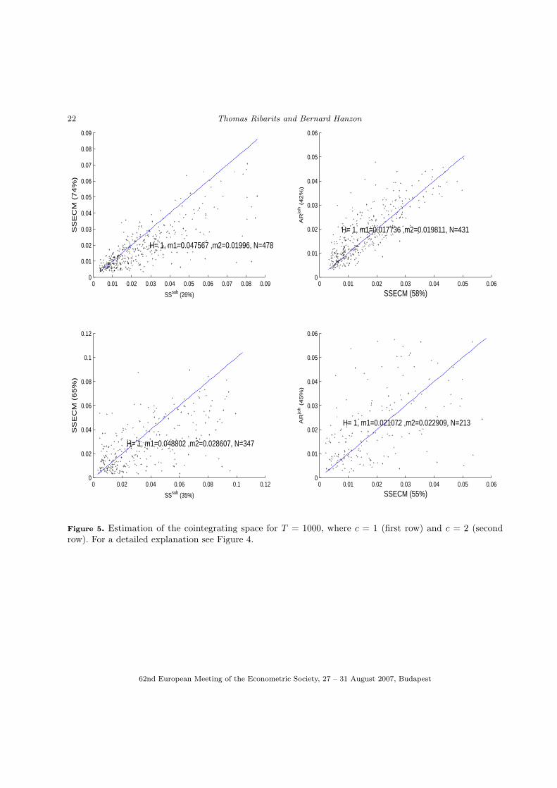
As expected, the gaps for T = 1000 are extremely small for any estimation approach. This can be explainedby the fact that the cointegrating space can be estimated super-consistently. In a pairwise comparison,however, SSECM takes the lead both relative to ARjoh and relative to SSsub; see Figure 5.
7.1.3. Predictive power of estimated systems In a final step, we also evaluated both AR and SSECM (andSSsub) estimates in terms of their predictive (i.e. true out-of-sample) performance. For T = 100 observations,we can conclude the following from Figure 6:
• The predictive power of SSECMs is better than the one of V AR models for all c = 0, 1, 2, 3. However,the t-tests indicate a clear superiority only for c = 3.• Comparing SSECM and SSsub, SSECM is better for c = 0 and c = 1, where the superiority is significant
for c = 0. Surprisingly, SSsub turns out to have lower out-of-sample mean squared errors for c = 2 andc = 3.
Note that the true innovation variance is given by Σ in (7.32) and det Σ = 0.0079. For T = 1000, thecomparisons remain unchanged, with the only difference that the MSEs (in absolute terms) are alreadyvery close to the theoretical value 0.0079. This is the reason why we have omitted to include another figurefor this case.
To sum it up, we see that if the data generating model is VARMA(1,1) – and can then also be representedin state-space form – then SSECMs offer a clear advantage over the classical VAR framework.
62nd European Meeting of the Econometric Society, 27 – 31 August 2007, Budapest
16 Thomas Ribarits and Bernard Hanzon
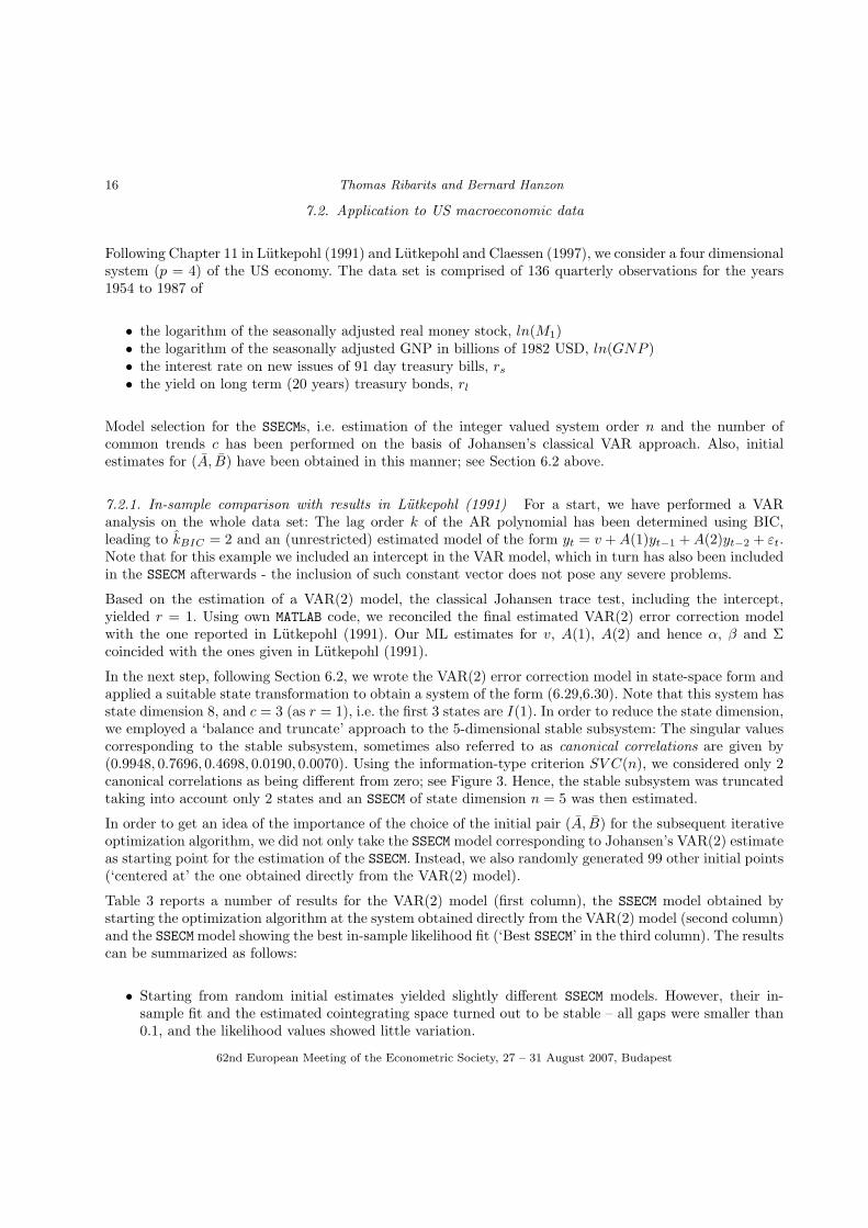
7.2. Application to US macroeconomic data
Following Chapter 11 in Lutkepohl (1991) and Lutkepohl and Claessen (1997), we consider a four dimensionalsystem (p = 4) of the US economy. The data set is comprised of 136 quarterly observations for the years1954 to 1987 of
• the logarithm of the seasonally adjusted real money stock, ln(M1)• the logarithm of the seasonally adjusted GNP in billions of 1982 USD, ln(GNP )• the interest rate on new issues of 91 day treasury bills, rs• the yield on long term (20 years) treasury bonds, rl
Model selection for the SSECMs, i.e. estimation of the integer valued system order n and the number ofcommon trends c has been performed on the basis of Johansen’s classical VAR approach. Also, initialestimates for (A, B) have been obtained in this manner; see Section 6.2 above.
7.2.1. In-sample comparison with results in Lutkepohl (1991) For a start, we have performed a VARanalysis on the whole data set: The lag order k of the AR polynomial has been determined using BIC,leading to kBIC = 2 and an (unrestricted) estimated model of the form yt = v +A(1)yt−1 +A(2)yt−2 + εt.Note that for this example we included an intercept in the VAR model, which in turn has also been includedin the SSECM afterwards - the inclusion of such constant vector does not pose any severe problems.
Based on the estimation of a VAR(2) model, the classical Johansen trace test, including the intercept,yielded r = 1. Using own MATLAB code, we reconciled the final estimated VAR(2) error correction modelwith the one reported in Lutkepohl (1991). Our ML estimates for v, A(1), A(2) and hence α, β and Σcoincided with the ones given in Lutkepohl (1991).
In the next step, following Section 6.2, we wrote the VAR(2) error correction model in state-space form andapplied a suitable state transformation to obtain a system of the form (6.29,6.30). Note that this system hasstate dimension 8, and c = 3 (as r = 1), i.e. the first 3 states are I(1). In order to reduce the state dimension,we employed a ‘balance and truncate’ approach to the 5-dimensional stable subsystem: The singular valuescorresponding to the stable subsystem, sometimes also referred to as canonical correlations are given by(0.9948, 0.7696, 0.4698, 0.0190, 0.0070). Using the information-type criterion SV C(n), we considered only 2canonical correlations as being different from zero; see Figure 3. Hence, the stable subsystem was truncatedtaking into account only 2 states and an SSECM of state dimension n = 5 was then estimated.
In order to get an idea of the importance of the choice of the initial pair (A, B) for the subsequent iterativeoptimization algorithm, we did not only take the SSECM model corresponding to Johansen’s VAR(2) estimateas starting point for the estimation of the SSECM. Instead, we also randomly generated 99 other initial points(‘centered at’ the one obtained directly from the VAR(2) model).
Table 3 reports a number of results for the VAR(2) model (first column), the SSECM model obtained bystarting the optimization algorithm at the system obtained directly from the VAR(2) model (second column)and the SSECM model showing the best in-sample likelihood fit (‘Best SSECM’ in the third column). The resultscan be summarized as follows:
• Starting from random initial estimates yielded slightly different SSECM models. However, their in-sample fit and the estimated cointegrating space turned out to be stable – all gaps were smaller than0.1, and the likelihood values showed little variation.
62nd European Meeting of the Econometric Society, 27 – 31 August 2007, Budapest
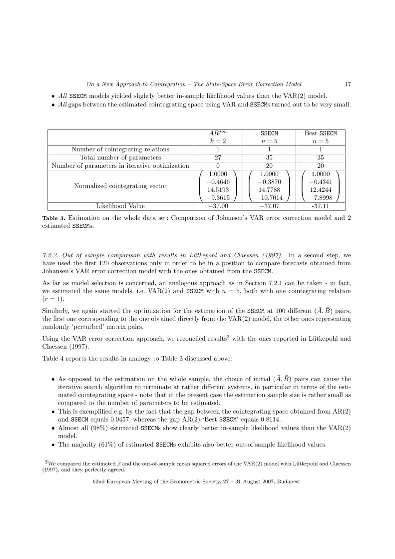
On a New Approach to Cointegration – The State-Space Error Correction Model 17
• All SSECM models yielded slightly better in-sample likelihood values than the VAR(2) model.• All gaps between the estimated cointegrating space using VAR and SSECMs turned out to be very small.
ARjoh SSECM Best SSECMk = 2 n = 5 n = 5
Number of cointegrating relations 1 1 1Total number of parameters 27 35 35
Number of parameters in iterative optimization 0 20 20
Normalized cointegrating vector
1.0000−0.464614.5193−9.3615
1.0000−0.387014.7788−10.7014
1.0000−0.434112.4244−7.8998
Likelihood Value −37.00 −37.07 -37.11
Table 3. Estimation on the whole data set: Comparison of Johansen’s VAR error correction model and 2estimated SSECMs.
7.2.2. Out of sample comparison with results in Lutkepohl and Claessen (1997) In a second step, wehave used the first 120 observations only in order to be in a position to compare forecasts obtained fromJohansen’s VAR error correction model with the ones obtained from the SSECM.
As far as model selection is concerned, an analogous approach as in Section 7.2.1 can be taken - in fact,we estimated the same models, i.e. VAR(2) and SSECM with n = 5, both with one cointegrating relation(r = 1).
Similarly, we again started the optimization for the estimation of the SSECM at 100 different (A, B) pairs,the first one corresponding to the one obtained directly from the VAR(2) model, the other ones representingrandomly ‘perturbed’ matrix pairs.
Using the VAR error correction approach, we reconciled results3 with the ones reported in Lutkepohl andClaessen (1997).
Table 4 reports the results in analogy to Table 3 discussed above:
• As opposed to the estimation on the whole sample, the choice of initial (A, B) pairs can cause theiterative search algorithm to terminate at rather different systems, in particular in terms of the esti-mated cointegrating space - note that in the present case the estimation sample size is rather small ascompared to the number of parameters to be estimated.• This is exemplified e.g. by the fact that the gap between the cointegrating space obtained from AR(2)
and SSECM equals 0.0457, whereas the gap AR(2)-‘Best SSECM’ equals 0.8114.• Almost all (98%) estimated SSECMs show clearly better in-sample likelihood values than the VAR(2)
model.• The majority (61%) of estimated SSECMs exhibits also better out-of sample likelihood values.
3We compared the estimated β and the out-of-sample mean squared errors of the VAR(2) model with Lutkepohl and Claessen(1997), and they perfectly agreed.
62nd European Meeting of the Econometric Society, 27 – 31 August 2007, Budapest

18 Thomas Ribarits and Bernard Hanzon
• The gap between the estimated cointegrating space using VAR and SSECM turned out to be very smallfor the majority of estimated SSECMs. However, the ones with particularly good in-sample (and out-ofsample) fits, exhibited cointegrating relations very different from the one obtained from the AR(2)model.
We would like to add two remarks: First, comparing the VAR(2) estimate obtained on the whole data set inSection 7.2.1 with the one obtained now on the first 120 data points yields already a considerable differencein terms of the cointegrating space: Using the VAR(2) model in both cases, the gap turns out to be 0.3.Second, we have observed also surprisingly big changes in the estimation of β in VAR(k) estimates when kwas further increased. In the light of these observations it then did not turn out to be too surprising thatcomparing the β estimates for the VAR(2) and the best SSECM estimate also yielded big differences.
ARjoh SSECM Best SSECMk = 2 n = 5 n = 5
Normalized cointegrating vector
1.0000−0.3430−16.720019.3500
1.0000−0.3889−12.553715.8996
1.0000−0.56785.40800.3294
In-sample Likelihood Value −37.55 −37.59 −37.74
Out Of Sample Likelihood Value −35.54 −35.48 −36.39
Table 4. Estimation on the first 120 data points: Comparison of Johansen’s VAR error correction model and2 estimated SSECMs.
Finally, in Lutkepohl and Claessen (1997) the authors extend the VAR(2) analysis to the VARMA case andpresent also out-of sample mean squared errors for each component. Comparing their estimated VARMAmodel with the SSECMs presented in this paper yields the following results:
• In all but 3 SSECM models ln(M1), rs and rl are forecasted more accurately than in the VARMA modelin Lutkepohl and Claessen (1997).• The VARMA model in Lutkepohl and Claessen (1997) yields better forecasts for ln(GNP ) than almost
all SSECMs.
We want to stress that state-space modeling, in particular in terms of SSECMs, offers a number of advantagesover VARMA models; see the conclusions presented in Section 8 below.
8. SUMMARY AND CONCLUSIONS
This paper has introduced a new approach towards I(1) cointegration analysis. The basic idea was togeneralize classical VAR cointegration to the state-space framework, leading to the introduction of thestate-space error correction model SSECM. This generalization mimics the classical VAR case as much aspossible. In fact, VAR models are embedded as a special case within the new framework – the suggestedestimation algorithm does not encounter any (numerical) difficulties if the model is of VAR-type.
The main contributions of this paper are the following:
• We have introduced the state-space error correction model SSECM.
62nd European Meeting of the Econometric Society, 27 – 31 August 2007, Budapest

On a New Approach to Cointegration – The State-Space Error Correction Model 19
• A complete treatment of how to estimate SSECMs by (pseudo-)maximum likelihood methods has beengiven. We have ‘concentrated out’ as many parameters as possible in order to reduce the dimensionalityin the non-linear likelihood optimization problem.• We have used a new data-driven local parametrization (DDLC) for the estimation of SSECMs.• The gradient of the concentrated likelihood function, if existing, can be efficiently computed by using
the original (non-concentrated) likelihood function. In any case, our suggested ‘adapted’ gradientalgorithm can only get stuck at critical points which are also critical points of the original likelihoodfunction.• A simulation study has been conducted, showing the potential of the new approach. The true model
being VARMA(1,1), SSECMs provided better estimates of the cointegrating spaces and better forecaststhan classical VAR models.• An application to US macroecomic data has been presented. The estimated SSECMs outperformed
the VAR estimates both in terms of in-sample and out-of-sample properties. A brief comparison toVARMA estimates shows advantages for SSECMs.
Finally, it should be stressed that SSECMs, despite representing the same model class as VARMA models,offer a number of advantages over the latter:
• Available estimation techniques for state-space models are much simpler from the point of view ofcomputational implementation. This is mainly due to the fact that the innovations can be computedby a simple inversion of the state-space system (or, in general, the Kalman filter), whereas one has toresort to some sort of multi-step procedure to obtain the innovations in the VARMA framework.• Using SSECMs in combination with a data-driven local parametrization, one can clearly circumvent the
usage of canonical forms which often show considerable drawbacks:
– The usage of canonical forms often leads to numerical difficulties when employing a gradient-basedsearch algorithm.
– Also, they may be very complex in nature; see e.g. the Echelon canonical form for the VARMAmodel in Lutkepohl and Claessen (1997).
– Their application may require a great effort already in the model selection stage: The authors inLutkepohl and Claessen (1997), for instance, estimated 2401 (!) initial models (corresponding todifferent Kronecker indices) in the model selection stage when we only estimated a single one (fordetermining the order n).
– Finally, VARMA model selection using the Echelon canonical form might end up with a chosenKronecker index which is incompatible with the estimated cointegrating rank r.
• Using SSECMs, one concentrates out as many parameters as possible and will, in general, thereforeend up with a significantly lower number of parameters appearing in the final non-linear optimizationproblem as compared to the VARMA case.• For SSECMs, the remaining free parameters in the nonlinar optimization problem all correspond to a
stable system. Note that parameters in the non-linear optimization problem corresponding to both sta-ble and non-stable systems (as in the VARMA case) may cause convergence problems for an algorithmin practice as level sets may become very distorted.• Finally, cointegration analysis using SSECMs is conceptually very close to the well known and classical
VAR approach. One can therefore also use classical VAR cointegration techniques to directly obtaininitial estimates4, and this fact should also allow practicioners to quickly adapt themselves to theSSECMs.
4As a side remark, we do not rely upon a technical condition called ‘strict minimum phase assumption’ for an initial estimateof (A,B,C) in our approach.
62nd European Meeting of the Econometric Society, 27 – 31 August 2007, Budapest

20 Thomas Ribarits and Bernard Hanzon
REFERENCES
Bauer, D. and M. Wagner (2002). Estimating cointegrated systems using subspace algorithms. Journal ofEconometrics 111 (1), 47–84.
Bauer, D. and M. Wagner (2003, July). A canonical form for unit root processes in the state spaceframework. Diskussionsschriften dp0312, Universitaet Bern, Volkswirtschaftliches Institut. available at:http://ideas.repec.org/p/ube/dpvwib/dp0312.html.
Dai, Q. and K. Singleton (2000, October). Specification analysis of affine term structure models. TheJournal of Finance 55 (5), 1943–1978.
Johansen, S. (1995). Likelihood-Based Inference in Cointegrated Vector Auto-Regressive Models. OxfordUniversity Press.
Lutkepohl, H. (1991). Introduction to Multiple Time Series Analysis. Berlin, Heidelberg: Springer.Lutkepohl, H. and H. Claessen (1997). Analysis of cointegrated VARMA processes. Journal of Economet-
rics 80, 223–239.McKelvey, T., A. Helmersson, and T. Ribarits (2004). Data driven local coordinates for multivariable linear
systems and their application to system identification. Automatica 40 (9), 1629–1635.Ribarits, T., M. Deistler, and B. Hanzon (2004). On new parametrization methods for the estimation of
state-space models. Intern. Journal of Adaptive Control and Signal Processing, Special Issue on Subspace-based Identification 18, 717–743.
Ribarits, T., M. Deistler, and B. Hanzon (2005). An analysis of separable least squares data driven localcoordinates for maximum likelihood estimation of linear systems. Automatica, ‘Special Issue on Data-Based Modeling and System Identification’ 41 (3), 531–544.
Ribarits, T., M. Deistler, and T. McKelvey (2004). An analysis of the parametrization by data driven localcoordinates for multivariable linear systems. Automatica 40 (5), 789–803.
Ribarits, T. and B. Hanzon (2005, January). The state-space error correction model: Definition, estimationand model selection. Mimeo, Technische Universitaet Wien. Available upon request.
Saikkonen, P. and R. Luukkonen (1997). Testing cointegration in infinite order vector autoregressive pro-cesses. Journal of Econometrics 81, 93–126.
Scherrer, W. (2002). Local optimality of minimum phase balanced truncation. In Proceedings of the 15thIFAC World Congress, Barcelona, Spain.
62nd European Meeting of the Econometric Society, 27 – 31 August 2007, Budapest

On a New Approach to Cointegration – The State-Space Error Correction Model 21
0 0.1 0.2 0.3 0.4 0.5 0.6 0.7 0.80
0.1
0.2
0.3
0.4
0.5
0.6
0.7
0.8
SSsub (19%)
SS
EC
M (
81
%)
H= 1, m1=0.25728 ,m2=0.10507, N=323
0 0.05 0.1 0.15 0.2 0.25 0.3 0.35 0.4 0.450
0.05
0.1
0.15
0.2
0.25
0.3
0.35
0.4
0.45
SSECM (56%)A
Rjo
h (
44%
)
H= 0, m1=0.13132 ,m2=0.1345, N=77
0 0.2 0.4 0.6 0.8 10
0.1
0.2
0.3
0.4
0.5
0.6
0.7
0.8
0.9
1
SSsub (43%)
SS
EC
M (
57
%)
H= 1, m1=0.63218 ,m2=0.60266, N=121
0 0.2 0.4 0.6 0.8 10
0.1
0.2
0.3
0.4
0.5
0.6
0.7
0.8
0.9
1
SSECM (73%)
AR
joh (
27%
)
H= 1, m1=0.30746 ,m2=0.34634, N=33
Figure 4. Estimation of the cointegrating space for T = 100, where c = 1 (first row) and c = 2 (second row).The left column compares the gap between estimated and true cointegrating space, where estimation is doneby SSECM and SSsub. The right column provides the same information, comparing ARjoh and SSECM. The‘winner’ of each comparison, i.e. the estimation approach yielding a lower gap in the majority (> 50%)) ofthe estimation runs, is indicated by the usage of a larger font size for the corresponding axis label; m1 andm2 denote the arithmetic mean of the gaps for the estimation approach indicated on the x-axis and they-axis, respectively; N corresponds to the number of estimation runs (out of 500) where both estimationapproaches of the comparison led to a correct specification of c; H = 0 indicates that a t-test (performed onthe logarithms of the gaps) does not reject the null hypothesis of equal gap means for the two estimationapproaches in the comparison, whereas H = 1 indicates a rejection in favour of the alternative hypothesisthat the ‘winner’ of the comparison (as defined above) has indeed a lower mean gap (left-sided t-tests havebeen performed).
62nd European Meeting of the Econometric Society, 27 – 31 August 2007, Budapest
22 Thomas Ribarits and Bernard Hanzon
0 0.01 0.02 0.03 0.04 0.05 0.06 0.07 0.08 0.090
0.01
0.02
0.03
0.04
0.05
0.06
0.07
0.08
0.09
SSsub (26%)
SS
EC
M (
74
%)
H= 1, m1=0.047567 ,m2=0.01996, N=478
0 0.01 0.02 0.03 0.04 0.05 0.060
0.01
0.02
0.03
0.04
0.05
0.06
SSECM (58%)A
Rjo
h (
42%
)
H= 1, m1=0.017736 ,m2=0.019811, N=431
0 0.02 0.04 0.06 0.08 0.1 0.120
0.02
0.04
0.06
0.08
0.1
0.12
SSsub (35%)
SS
EC
M (
65
%)
H= 1, m1=0.048802 ,m2=0.028607, N=347
0 0.01 0.02 0.03 0.04 0.05 0.060
0.01
0.02
0.03
0.04
0.05
0.06
SSECM (55%)
AR
joh (
45%
)
H= 1, m1=0.021072 ,m2=0.022909, N=213
Figure 5. Estimation of the cointegrating space for T = 1000, where c = 1 (first row) and c = 2 (secondrow). For a detailed explanation see Figure 4.
62nd European Meeting of the Econometric Society, 27 – 31 August 2007, Budapest

On a New Approach to Cointegration – The State-Space Error Correction Model 23
0.006 0.008 0.01 0.012 0.014 0.016 0.018 0.02 0.0220.005
0.01
0.015
0.02
0.025
SSsub (45.5487%)
SS
EC
M (
54.4
513%
)
H= 1, m1=0.011786 ,m2=0.011683, N=483
0.006 0.008 0.01 0.012 0.014 0.016 0.018 0.020.005
0.01
0.015
0.02
SSECM (71.5618%)
AR
joh (
28.4
382%
)
H= 0, m1=0.011673 ,m2=0.011835, N=429
0.005 0.01 0.015 0.02 0.025 0.03 0.0350
0.01
0.02
0.03
0.04
SSsub (45.2012%)
SS
EC
M (
54.7
988%
)
H= 0, m1=0.018907 ,m2=0.018067, N=323
0.005 0.01 0.015 0.02 0.025 0.03 0.035 0.04 0.0450
0.02
0.04
SSECM (64.9351%)
AR
joh (
35.0
649%
)
H= 0, m1=0.020364 ,m2=0.018526, N=77
0 0.02 0.04 0.06 0.08 0.1 0.12 0.140
0.05
0.1
0.15
0.2
SSsub (82.6446%)
SS
EC
M (
17.3
554%
)
H= 1, m1=0.02647 ,m2=0.045285, N=121
0.01 0.02 0.03 0.04 0.05 0.06
0.02
0.04
0.06
SSECM (63.6364%)
AR
joh (
36.3
636%
)
H= 0, m1=0.023778 ,m2=0.030822, N=33
0.007 0.008 0.009 0.01 0.011 0.012 0.013 0.014 0.015 0.0160.006
0.008
0.01
0.012
0.014
0.016
SSsub (75%)
SS
EC
M (
25%
)
H= 1, m1=0.0095381 ,m2=0.011657, N=12
0.008 0.01 0.012 0.014 0.016 0.018 0.02 0.0220.005
0.01
0.015
0.02
0.025
SSECM (88.8889%)
AR
joh (
11.1
111%
)
H= 1, m1=0.01148 ,m2=0.015244, N=9
Figure 6. Out-of-sample mean squared errors for T = 100, where c = 0 (first row), c = 1 (second row), c = 2(third row) and c = 3 (last row). The estimated models have been used for one-step-ahead forecasts over 200periods, yielding out-of-sample forecast errors ε501, . . . , ε700, say. In this figure, MSE = det 1
200
∑700t=501 εtε
′t
are compared for estimated models where c has been correctly specified. The left column compares theMSE for SSECM and SSsub, the right column for ARjoh and SSECM. The ‘winner’ of each comparison, i.e.the estimation approach yielding a lower MSE in the majority (> 50%)) of the estimation runs, is indicatedby the usage of a larger font size for the corresponding axis label; m1 and m2 denote the arithmetic mean ofthe MSEs for the estimation approach indicated on the x-axis and the y-axis, respectively; N correspondsto the number of estimation runs (out of 500) where both estimation approaches of the comparison led to acorrect specification of c; H = 0 indicates that a t-test does not reject the null hypothesis of equal MSEmeans for the two estimation approaches in the comparison, whereas H = 1 indicates a rejection in favourof the alternative hypothesis that the ‘winner’ of the comparison (as defined above) has indeed a lower meanMSE (left-sided t-tests have been performed).
62nd European Meeting of the Econometric Society, 27 – 31 August 2007, Budapest