on a kind of noether symmetries and conservation laws in k
TRANSCRIPT

On a kind of Noether symmetries and conservation laws in k-cosymplectic field theoryJuan Carlos Marrero, Narciso Román-Roy, Modesto Salgado, and Silvia Vilariño Citation: J. Math. Phys. 52, 022901 (2011); doi: 10.1063/1.3545969 View online: http://dx.doi.org/10.1063/1.3545969 View Table of Contents: http://jmp.aip.org/resource/1/JMAPAQ/v52/i2 Published by the American Institute of Physics. Related ArticlesSubstituting fields within the action: Consistency issues and some applications J. Math. Phys. 51, 122903 (2010) Loop vertex expansion for 2k theory in zero dimension J. Math. Phys. 51, 092304 (2010) Rigid symmetries and conservation laws in non-Lagrangian field theory J. Math. Phys. 51, 082902 (2010) Perturbative quantum field theory via vertex algebras J. Math. Phys. 50, 112304 (2009) The method of Ostrogradsky, quantization, and a move toward a ghost-free future J. Math. Phys. 50, 113508 (2009) Additional information on J. Math. Phys.Journal Homepage: http://jmp.aip.org/ Journal Information: http://jmp.aip.org/about/about_the_journal Top downloads: http://jmp.aip.org/features/most_downloaded Information for Authors: http://jmp.aip.org/authors
Downloaded 21 Nov 2011 to 147.83.95.33. Redistribution subject to AIP license or copyright; see http://jmp.aip.org/about/rights_and_permissions

JOURNAL OF MATHEMATICAL PHYSICS 52, 022901 (2011)
On a kind of Noether symmetries and conservation lawsin k-cosymplectic field theory
Juan Carlos Marrero,1,a) Narciso Roman-Roy,2,b) Modesto Salgado,3,c)
and Silvia Vilarino4,d)
1Dept. Matematica Fundamental Facultad de Matematicas. Universidad de la Laguna,38071-La Laguna, Tenerife. Spain2Dept. Matematica Aplicada IV. Edificio C-3, Campus Norte UPC, 08034-Barcelona. Spain3Dept. Xeometrıa e Topoloxıa, Facultade de Matematicas. Universidade de Santiago deCompostela. 15782-Santiago de Compostela. Spain4Dept. Matematicas, Facultade de Ciencias. Universidad de A Coruna. 15071-A Coruna.Spain
(Received 16 September 2010; accepted 31 December 2010; published online 4 February2011)
This paper is devoted to studying symmetries of certain kinds of k-cosymplecticHamiltonian systems in first-order classical field theories. Thus, we introduce aparticular class of symmetries and study the problem of associating conservationlaws to them by means of a suitable generalization of Noether’s theorem. C© 2011American Institute of Physics. [doi:10.1063/1.3545969]
I. INTRODUCTION
The k-cosymplectic formalisms is one of the simplest geometric frameworks for describing first-order classical field theories. It is the generalization to field theories of the standard cosymplecticformalism for nonautonomous mechanics,9, 10 and it describes field theories involving the coordinatesin the basis on the Lagrangian and on the Hamiltonian. The foundations of the k-cosymplecticformalism are the k-cosymplectic manifolds.9, 10
Historically, it is based on the so-called polysymplectic formalism developed by Gunther,16
who introduced polysymplectic manifolds. A refinement of this concept led to definek-symplectic manifolds,2–4 which are polysymplectic manifolds admitting Darboux-typecoordinates.8 (Other different polysymplectic formalisms for describing field theories have beenalso proposed.13, 17, 22, 25, 26, 29)
The natural extension of the k-symplectic manifolds is the k-cosymplectic manifolds. All of thisis discussed in Sec. II, which is devoted to make a review on the main features and characteristicsof k-cosymplectic manifolds and of k-cosymplectic Hamiltonian systems. We also introduce thenotions of almost standard k-cosymplectic manifold, which are those that we are interested in thispaper.
The main objective of this paper is to study symmetries and conservation laws on the first-orderclassical field theories, from the Hamiltonian viewpoint, using the k-cosymplectic description, andconsidering only the regular case. These problems have been treated for k-symplectic field theoriesin Refs. 23 and 28, generalizing the results obtained for nonautonomous mechanical systems (see, inparticular, Ref. 6, and references quoted therein).We further remark that the problem of symmetriesin field theory has also been analyzed using other geometric frameworks, such as the multisymplecticmodels (see, for instance, Refs. 5, 7, 12, 14, 15, 18, and 19).
In this way, in Sec. III we recover the idea of conservation law or conserved quantity. Then,we introduce a particular kind of symmetries for (almost-standard) k-cosymplectic Hamiltonian
a)Electronic mail: [email protected])Electronic mail: [email protected])Electronic mail: [email protected])Electronic mail: [email protected].
0022-2488/2011/52(2)/022901/20/$30.00 C©2011 American Institute of Physics52, 022901-1
Downloaded 21 Nov 2011 to 147.83.95.33. Redistribution subject to AIP license or copyright; see http://jmp.aip.org/about/rights_and_permissions

022901-2 Marrero et al. J. Math. Phys. 52, 022901 (2011)
systems, essentially those transformations preserving the k-cosymplectic structure, which allowsus to state a generalization of Noether’s theorem. The definition of these so-called k-cosymplecticNoether symmetries is inspired in the ideas introduced by Albert in his study of symmetries for thecosymplectic formalism of autonomous mechanical systems.1
Finally, as an example, in Sec. IV we describe briefly the k-cosymplectic quadratic Hamiltoniansystems and we analyze some Noether symmetries for these kinds of systems (in particular, for thewave equation).
In this paper, manifolds are real, paracompact, connected and C∞, maps are C∞, and sum overcrossed repeated indices is understood.
II. GEOMETRIC ELEMENTS: HAMILTONIAN k-COSYMPLECTIC FORMALIS
(The contents of this section can be seen in more detail in Ref. 10.)
A. k-vector fields and integral sections
Let M be an arbitrary manifold, T 1k M be the Whitney sum T M⊕ k. . . ⊕T M of k copies of
T M , and τ : T 1k M −→ M be its canonical projection. T 1
k M is usually called the tangent bundle ofk1-velocities of M .
Definition 1: A k-vector field on M is a section X : M −→ T 1k M of the projection τ .
Giving a k-vector field X is equivalent to giving a family of k vector fields X1, . . . , Xk on Mobtained by projecting X onto every factor; that is, X A = τA ◦ X, where τA : T 1
k M → T M is thecanonical projection onto the Ath-copy T M of T 1
k M (1 ≤ A ≤ k). For this reason we will denote ak-vector field by X = (X1, . . . , Xk).
Definition 2: An integral section of the k-vector field (X1, . . . , Xk) passing through a pointx ∈ M is a map ψ : U0 ⊂ Rk → M, defined on some neighborhood U0 of 0 ∈ Rk , such that
ψ(0) = x , ψ∗(t)
(∂
∂t A
∣∣∣t
)= X A(ψ(t)) (for every t ∈ U0),
A k-vector field X is integrable if every point of M belongs to the image of an integral section of X.
In coordinates, if X A = XiA
∂
∂qi, then ψ is an integral section of X if, and only if, the following
system of partial differential equations holds
∂ψ i
∂t A= Xi
A ◦ ψ.
We remark that a k-vector field X = (X1, . . . , Xk) is integrable if, and only if, the vectorfields X1, . . . , Xk generate a completely integrable distribution of rank k. This is the geometricexpression of the integrability condition of the preceding differential equation (see, for instance,Refs. 11 and 21).
Observe that, in case k = 1, this definition coincides with the definition of integral curve of avector field.
B. k-symplectic manifolds
The polysymplectic structures were introduced in Ref. 16 and the k-symplectic structures inRefs. 2 and 14.
Definition 3: Let M be a differentiable manifold of dimension N = n + kn.
1. A polysymplectic structure on M is a family (ωA0 ) (1 ≤ A ≤ k), where each ωA
0 ∈ �2(M) is aclosed form, such that,
∩kA=1 ker ωA
0 = {0}.
Downloaded 21 Nov 2011 to 147.83.95.33. Redistribution subject to AIP license or copyright; see http://jmp.aip.org/about/rights_and_permissions

022901-3 Noether symmetries in k-cosymplectic field theory J. Math. Phys. 52, 022901 (2011)
Then (M, ωA0 ) is called a polysymplectic manifold.
2. A k-symplectic structure on M is a family (ωA0 , V ) (1 ≤ A ≤ k), such that (M, ωA
0 ) is apolysymplectic manifold and V is an integrable nk-dimensional tangent distribution on Msatisfying that
ωA0 |V ×V = 0, f or every A.
Then (M, ωA0 , V ) is called a k-symplectic manifold.
The k-symplectic (respectively, polysymplectic) structure is exact if ωA0 = dθ A
0 , for all A.
Theorem 1: (Ref. 8). Let (ωA0 , V ) be a k-symplectic structure on M. For every point of M,
there exists a neighborhood U and local coordinates (qi , pAi ) (1 ≤ i ≤ n, 1 ≤ A ≤ k) such that,
on U,
ωA0 = dqi ∧ dpA
i , V =⟨
∂
∂p1i
, . . . ,∂
∂pki
⟩i=1,...,n
.
These are called Darboux or canonical coordinates of the k-symplectic manifold.The canonical model of a k-symplectic manifold is ((T 1
k )∗ Q, ωA0 , V ), where Q is an n-
dimensional differentiable manifold and (T 1k )∗ Q = T ∗ Q⊕ k. . . ⊕T ∗ Q is the Whitney sum of k
copies of the cotangent bundle T ∗ Q, which is usually called the bundle of k1-covelocities of Q (seeRef. 20). We have the natural projections
π A : (T1k)∗Q → T∗ Q
(q; α1q , . . . , α
kq ) �→ (q; αA
q ),
(πQ)1 : (T1k)∗Q → Q
(q; α1q , . . . , α
kq ) �→ q.
The manifold (T 1k )∗ Q can be identified with the manifold J 1(Q,Rk)0 of 1-jets of mappings from Q
to Rk with target at 0 ∈ Rk , that is,
J 1(Q,Rk)0 ≡ T ∗ Q⊕ k. . . ⊕T ∗ Q
j1q,0σQ ≡ (dσ 1
Q(q), . . . , dσ kQ(q)),
where σ AQ = π A
0 ◦ σQ : Q −→ R is the Ath component of σQ , and π A0 : Rk → R is the canonical
projection onto the A component.Here, (T1
k)∗Q is endowed with the canonical forms
θ A = (π A)∗θ0, ωA0 = (π A)∗ω0 = −(π A)∗dθ0,
where θ0 and ω0 = −dθ0 are the Liouville 1-form and the canonical symplectic form on T∗ Q.Obviously ωA
0 = −dθ A0 .
If (qi ) are local coordinates on U ⊂ Q, the induced coordinates (qi , pAi ) on (π1
Q)−1(U ) aregiven by
qi (q; α1q , . . . , α
kq ) = qi (q)
pAi (q; α1
q , . . . , αkq ) = αA
q
(∂
∂qi
∣∣∣q
).
Then we have
θ A0 = pA
i dqi , ωA0 = dqi ∧ dpA
i .
Thus, the triple ((T1k)∗ Q, ωA
0 , V ), where V = ker T(πQ)1, is a k-symplectic manifold, and the naturalcoordinates in (T1
k)∗Q are Darboux coordinates.
Downloaded 21 Nov 2011 to 147.83.95.33. Redistribution subject to AIP license or copyright; see http://jmp.aip.org/about/rights_and_permissions

022901-4 Marrero et al. J. Math. Phys. 52, 022901 (2011)
C. k-cosymplectic manifolds
Definition 4: Let M be a a differentiable manifold of dimension N = k + n + kn.
1. A polycosymplectic structure in M is a family (ηA, ωA), where ηA ∈ �1(M) and ωA
∈ �2(M) are closed forms satisfying that
(a) η1 ∧ . . . ∧ ηk �= 0.(b) (∩k
A=1 ker ωA∩kA=1 ker ηA) = {0}.
Then, (M, ηA, ωA) is said to be a polycosymplectic manifold.2. A k–cosymplectic structure in M is a family (ηA, ωA,V) such that (M, ηA, ωA) is a poly-
cosymplectic manifold, and V is an nk-dimensional integrable distribution on M, satisfyingthat
(a) ηA|V = 0.(b) ωA|V×V = 0.
Then, (M, ηA, ωA,V) is said to be a k–cosymplectic manifold.
The k-cosymplectic (respectively, polycosymplectic) structure is exact if ωA = dθ A, for all A.
For every k-cosymplectic structure (ηA, ωA,V) on M, there exists a family of k vector fields{RA} 1≤A≤k , which are called Reeb vector fields, characterized by the following conditions:9
i(RA)ηB = δBA , i(RA)ωB = 0; 1 ≤ A, B ≤ k .
Theorem 2: (Darboux Theorem).9 If M is a k–cosymplectic manifold, then for every point ofM there exists a local chart of coordinates (t A, qi , pA
i ), 1 ≤ A ≤ k, 1 ≤ i ≤ n, such that
ηA = dt A , ωA = dqi ∧ dpAi , RA = ∂
∂t A
V =⟨
∂
∂p1i, . . . , ∂
∂pki
⟩i=1,...,n
.
These are called Darboux or canonical coordinates of the k-cosymplectic manifold.The canonical model for k-cosymplectic manifolds is (Rk × (T 1
k )∗Q, ηA, ωA,V). The manifoldJ 1πQ of 1-jets of sections of the trivial bundle πQ : Rk × Q → Q is diffeomorphic toRk × (T 1
k )∗Q.We use also the following notation for the canonical projections:
(πQ)1 : Rk × (T 1k )∗ Q
(πQ )1,0−→ Rk × QπQ−→ Q
given by
πQ(t, q) = q, (πQ)1,0(t, α1q , . . . , α
kq ) = (t, q),
(πQ)1(t, α1q , . . . , α
kq ) = q,
with t ∈ Rk , q ∈ Q, and (α1q , . . . , α
kq ) ∈ (T 1
k )∗ Q.If (qi ) are local coordinates on U ⊆ Q, then the induced local coordinates (t A, qi , pA
i ) on[(πQ)1]−1(U ) = Rk × (T 1
k )∗U are given by
t A(t, α1q , . . . , α
kq ) = t A ; qi (t, α1
q , . . . , αkq ) = qi (q) ;
pAi (t, α1
q , . . . , αkq ) = αA
q
(∂
∂qi
∣∣∣q
).
On Rk × (T 1k )∗ Q, we define the differential forms
ηA = (π A1 )∗dt A , θ A = (π A
2 )∗θ0 , ωA = (π A2 )∗ω0 ,
Downloaded 21 Nov 2011 to 147.83.95.33. Redistribution subject to AIP license or copyright; see http://jmp.aip.org/about/rights_and_permissions
022901-5 Noether symmetries in k-cosymplectic field theory J. Math. Phys. 52, 022901 (2011)
where π A1 : Rk × (T 1
k )∗ Q → R and π A2 : Rk × (T 1
k )∗ Q → T ∗ Q are the projections defined by
π A1 (t, (α1
q , . . . , αkq )) = t A , π A
2 (t, (α1q , . . . , α
kq )) = αA
q ,
In local coordinates, we have
ηA = dt A , θ A =n∑
i=1
pAi dqi , ωA =
n∑i=1
dqi ∧ dpAi .
Moreover, let V = ker T (πQ)1,0. Then V =⟨
∂
∂p1i
, . . . ,∂
∂pki
⟩i=1,...,n
.
Hence (Rk × (T 1k )∗ Q, ηA, ωA,V) is a k-cosymplectic manifold, and the natural coordinates of
Rk × (T 1k )∗Q are Darboux coordinates for this canonical k-cosymplectic structure. Furthermore,{
∂
∂t A
}are the Reeb vector fields of this structure.
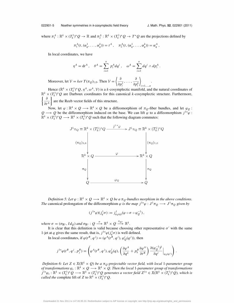
Now, let ϕ : Rk × Q −→ Rk × Q be a diffeomorphism of πQ-fiber bundles, and let ϕQ :Q −→ Q be the diffeomorphism induced on the base. We can lift ϕ to a diffeomorphism j1∗ϕ :Rk × (T 1
k )∗Q −→ Rk × (T 1k )∗Q such that the following diagram commutes:
Definition 5: Let ϕ : Rk × Q −→ Rk × Q be a πQ-bundles morphism in the above conditions.The canonical prolongation of the diffeomorphism ϕ is the map j1∗ϕ : J 1πQ −→ J 1πQ given by
( j1∗ϕ)( j1q σ ) := j1
ϕQ (q)(ϕ ◦ σ ◦ ϕ−1Q ) ,
where σ = (σRk , I dQ) and σRk : Qσ−→ Rk × Q
πRk−→ Rk .It is clear that this definition is valid because choosing other representative σ ′ with the same
1-jet at q gives the same result, that is, j1∗ϕ( j1q σ ) is well defined.
In local coordinates, if ϕ(t B, q j ) = (ϕA(t B, q j ), ϕiQ(q j )), then
j1∗ϕ(t B, q j , pBj ) =
(ϕA(t B, q j ), ϕ j
Q(q),
(∂ϕA
∂qk+ pB
k
∂ϕA
∂t B
)∂(ϕ−1
Q )k
∂qi
∣∣∣ϕQ (q j )
).
Definition 6: Let Z ∈ X(Rk × Q) be a πQ-projectable vector field, with local 1-parameter groupof transformations ϕs : Rk × Q −→ Rk × Q. Then the local 1-parameter group of transformationsj1∗ϕs : Rk × (T 1
k )∗ Q −→ Rk × (T 1k )∗ Q generates a vector field Z1∗ ∈ X(Rk × (T 1
k )∗ Q), which iscalled the complete lift of Z to Rk × (T 1
k )∗ Q.
Downloaded 21 Nov 2011 to 147.83.95.33. Redistribution subject to AIP license or copyright; see http://jmp.aip.org/about/rights_and_permissions

022901-6 Marrero et al. J. Math. Phys. 52, 022901 (2011)
If the local expression of Z ∈ X(Rk × Q) is Z = Z A ∂
∂t A+ Zi ∂
∂qi, then
Z1∗ = Z A ∂
∂t A+ Zi ∂
∂qi+
(d Z A
dqi− pA
j
d Z j
dqi
)∂
∂pAi
,
whered
dqidenotes the total derivative, that is,
d
dqi= ∂
∂qi+ pB
i
∂
∂t B.
D. k-cosymplectic Hamiltonian systems
Along this paper we are interested only in a kind of k-cosymplectic manifolds: those which areof the form M = Rk × M , where (M, ωA
0 , V ) is a generic k-symplectic manifold. Then, denotingby
πRk : Rk × M → Rk, πM : Rk × M → M
the canonical projections, we have the differential forms
ηA = π∗Rk dt A, ωA = π∗
MωA0 ,
and the distribution V in M defines a distribution V in M = Rk × M in a natural way. All theconditions given in Definition 4 are verified, and hence Rk × M is a k-cosymplectic manifold. Fromthe Darboux Theorem 1, we have local coordinates (t A, qi , pA
i ) in Rk × M .Observe that the standard model is a particular class of these kinds of k-cosymplectic manifolds,
where M = (T 1k )∗ Q.
Definition 7: These kinds of k-cosymplectic manifolds will be called almost-standardk-cosymplectic manifolds.
Consider an almost-standard k-cosymplectic manifold (Rk × M, ηA, ωA,V), and let H∈ C∞(Rk × M) be a Hamiltonian function. The couple (Rk × M, H ) is called a k-cosymplecticHamiltonian system.
We denote by XkH (Rk × M) the set of (local) k-vector fields X = (X1, . . . , Xk) on Rk × M
which are solutions to the equations
ηA(X B) = δAB ,
k∑A=1
i(X A)ωA = dH −k∑
A=1
RA(H )ηA. (1)
Since RA = ∂/∂t A and ηA = dt A, then we can write locally the above equations as follows:
dt A(X B) = δAB ,
k∑A=1
i(X A)ωA = dH −k∑
A=1
∂ H
∂t Adt A.
Furthermore, for a section ψ : I ⊂ Rk → Rk × M of the projection πRk , the Hamilton–deDonder-Weyl equations for this system are
k∑A=1
i
(ψ∗(t)
(∂
∂t A
∣∣∣t
))(ωA ◦ ψ) =
[dH −
k∑A=1
RA(H )ηA
]◦ ψ, (2)
In Darboux coordinates, if ψ(t) = (ψ A(t), ψ i (t), ψ Ai (t)), as ψ is a section of the projection πRk , it
implies that ψ A(t) = t A the above equations lead to the equations
∂ H
∂qi= −
k∑A=1
∂ψ Ai
∂t A,
∂ H
∂pAi
= ∂ψ i
∂t A. (3)
The relation between Equations (1) and (2) is given by the following:
Downloaded 21 Nov 2011 to 147.83.95.33. Redistribution subject to AIP license or copyright; see http://jmp.aip.org/about/rights_and_permissions

022901-7 Noether symmetries in k-cosymplectic field theory J. Math. Phys. 52, 022901 (2011)
Theorem 3: Let X = (X1, . . . , Xk) ∈ XkH (Rk × M) [i.e., it is a k-vector field on Rk × M which
is a solution to the geometric Hamiltonian equations (1)]. If a section ψ : Rk → Rk × M of πRk isan integral section of X, then ψ is a solution to the Hamilton–de Donder-Weyl field equations (2).
Proof: Let X = (X1, . . . , Xk) ∈ XkH (Rk × M) be locally given by
X A = (X A)B ∂
∂t B + (X A)i ∂
∂qi + (X A)Bi
∂
∂pBi
,
then, from (1) we obtain
(X A)B = δBA ,
∂ H
∂pAi
= (X A)i ,∂ H
∂qi= −
k∑A=1
(X A)Ai , (4)
and if ψ : Rk → Rk × M , locally given by ψ(t) = (t A, ψ i (t), ψ Ai (t)), is an integral section of X ,
then
∂ψ i
∂t B= (X B)i ,
∂ψ Ai
∂t B= (X B)A
i .
Therefore, from (4) we obtain that ψ(t) is a solution to the Hamiltonian field equations (3). �And, conversely, we have the following:
Lemma 1: If a section ψ : Rk → Rk × M of πRk is a solution to the Hamilton–de Donder-Weylequation (2) and ψ is an integral section of X = (X1, . . . , Xk), then X = (X1, . . . , Xk) is solutionto the equations (1) at the points of the image of ψ .
Proof: We must prove that
∂ H
∂pAi
(ψ(t)) = (X A)i (ψ(t)) ,
∂ H
∂qi(ψ(t)) = −
k∑A=1
(X A)Ai (ψ(t)) , (5)
now as ψ(t) = (t A, ψ i (t), ψ Ai (t)) is integral section of X we have that
∂ψ i
∂t B(t) = (X B)i (ψ(t)),
∂ψ Ai
∂t B(t) = (X B)A
i (ψ(t)) . (6)
As ψ is a solution to the Hamilton–de Donder-Weyl equation (3) then, from (6), wededuce (5). �
We cannot claim that X ∈ XkH (Rk × M) because we cannot assure that X is a solution to the
equations (1) everywhere in Rk × M .
Proposition 1: If ψ : U0 ⊂ Rk −→ Rk × M is a solution to the Hamilton–de Donder–Weylequation (2), then for each t ∈ U0 there exist a neighborhood Ut of t and a k-vector field Xt
= (Xt1, . . . , Xt
k) on ψ(Ut ) which is solution to the equations (1) in ψ(Ut ).
Proof: If ψ : U0 ⊂ Rk → Rk × M is a solution to the Hamilton–de Donder-Weyl equation (2)then for every t ∈ U0 there exists a neighborhood Ut ⊂ U0 of t , and a neighborhood coordinatesystem (Wt , s A, qi , pA
i ) of ψ(t), such that ψ(Ut ) = Wt ⊂ ψ(U0), and ψ(s) = (s, ψ i (s), ψ Ai (s)) for
every s ∈ Ut .As ψ |Ut : Ut → Wt is an injective immersion (ψ is a section and hence its image is an embedded
submanifold), we can define a k-vector field Xt = (Xt1, . . . , Xt
k) in ψ(Ut ) as follows:
XtA(ψ(s)) = ψ∗(s)
( ∂
∂s A
∣∣∣s
), s ∈ Ut ,
and so ψ |Ut is an integral section of Xt . Then, from Lemma 1, one obtains that Xt is solution to theequations (1) in ψ(Ut ). �
Downloaded 21 Nov 2011 to 147.83.95.33. Redistribution subject to AIP license or copyright; see http://jmp.aip.org/about/rights_and_permissions
022901-8 Marrero et al. J. Math. Phys. 52, 022901 (2011)
Remark: It should be noticed that, in general, equations (1) do not have a single solution. Infact, if (M, ηA, ωA,V) is a k-cosymplectic manifold we can define the vector bundle morphism,
ω� : T 1k M −→ T ∗M
(X1, . . . , Xk) �→k∑
A=1
i(X A)ωA
and, denoting by Mk(R) the space of matrices of order k whose entries are real numbers, the vectorbundle morphism
η� : T 1k M −→ M × Mk(R)
(X1, . . . , Xk) �→ (τ (X1, . . . , Xk), ηA(X B)) .
We denote by the same symbols ω�, η� their natural extensions to vector fields and forms.Now, let H : M → R be a real C∞-function on M. Then, as in the case of an almost-
standard k-cosymplectic manifold, we can consider the set XkH (M) of the (local) k-vector fields
X = (X1, . . . , Xk) on M which are solutions to the equations
ηA(X B) = δAB ,
k∑A=1
i(X A)ωA = d H −k∑
A=1
RA(H )ηA. (7)
Moreover, we may prove the following result:
Proposition 2: The solutions to Eqs. (7) are the sections of an affine bundle of rank (k − 1)(kn+ n) which is modeled on the vector sub-bundle ker ω� ∩ ker η� of T 1
k M.
Proof: We consider the vector sub-bundle ker η� of T 1k M and the vector bundle morphism
ω�|ker η� : ker η� → T ∗M.
It is clear that this morphism takes values in the vector sub-bundle ∩kA=1〈RA〉0 of T ∗M, where 〈RA〉0
is the vector sub-bundle of T ∗M whose fiber at the point x ∈ M is {α ∈ T ∗x M/α(RA(x)) = 0}.
Furthermore, we have that
ker(ω�|ker η� ) = ker ω� ∩ ker η�.
We will prove that
ω�|ker η� : ker η� → ∩kA=1〈RA〉0
is an epimorphism of vector bundles. For this purpose, we will see that the dual morphism
(ω�|ker η� )∗ : (∩kA=1〈RA〉0)∗ → (ker η�)∗
is a monomorphism of vector bundles.First, it is clear that the dual bundle to ∩k
A=1〈RA〉0 (respectively, ker η�) may be identifiedwith the vector bundle whose fiber at the point x ∈ M is ∩k
A=1〈ηA(x)〉0 [respectively, {(α1, . . . , αk)∈ ((T 1
k )∗M)x/αA(RB(x)) = 0, for all A, B}]. Under these identifications, the morphism ω�
| ker η� isgiven by
(ω�|ker η� )∗(v) = (i(v)ω1(x), . . . , i(v)ωk(x)) ,
for v ∈ ∩kA=1〈ηA(x)〉0. Thus, (ω�|ker η� )∗ is a monomorphism of vector bundles. Then ω
�
ker η� :
ker η� → ∩kA=1〈RA〉0 is an epimorphism of vector bundles.
So, as the rank of the vector bundle ker η� (respectively, ∩kA=1〈RA〉0) is k(kn + n) (respectively,
kn + n), we deduce that the rank of the vector bundle ker ω� ∩ ker η� is (k − 1)(kn + n).Furthermore, if (X1, . . . , Xk) is a particular solution of Eqs. (1) and Z is a section of
the vector bundle ker ω� ∩ ker η� → M then (X1, . . . , Xk) + Z also is a solution of theseequations. In addition, if X′ and X are solutions of Eqs. (1) then Z = X′ − X is a section ofthe vector bundle ker ω� ∩ ker η� → M.
Downloaded 21 Nov 2011 to 147.83.95.33. Redistribution subject to AIP license or copyright; see http://jmp.aip.org/about/rights_and_permissions
022901-9 Noether symmetries in k-cosymplectic field theory J. Math. Phys. 52, 022901 (2011)
Finally, if (t A, qi , pAi ) are Darboux coordinates in a neighborhood Ux of each point x ∈ M,
then we may define a local k-vector field on Ux that satisfies (7). For instance, we can put
(X1)1i = ∂ H
∂qi, (X A)B
i = 0 (for A �= 1 �= B), (X A)i = ∂ H
∂pAi
.
Now one can construct a global k-vector field, which is a solution of (1), by using a partition of unityin the manifold M (see Ref. 9). �
III. SYMMETRIES FOR k-COSYMPLECTIC HAMILTONIAN SYSTEMS
A. Symmetries and conservation laws
Let (Rk × M, H ) be a k-cosymplectic Hamiltonian system. First, following Ref. 27, we intro-duce the next definition:
Definition 8: A conservation law for the Hamilton–de Donder-Weyl equations (2) is a mapF = (F1, . . . ,F k) : Rk × M −→ Rk such that the divergence of
F ◦ ψ = (F1 ◦ ψ, . . . ,F k ◦ ψ) : U0 ⊂ Rk −→ Rk
is zero for every solution ψ to the Hamilton–de Donder-Weyl equations (2); that is for all t ∈ U0
⊂ Rk ,
0 = [Div(F ◦ ψ)](t) =k∑
A=1
∂(F A ◦ ψ)
∂t A
∣∣∣t
=k∑
A=1
ψ∗(t)( ∂
∂t A
∣∣∣t
)(F A) . (8)
Proposition 3: The map F = (F1, . . . ,F k) : Rk × M −→ Rk defines a conservation lawif, and only if, for every integrable k-vector field X = (X1, . . . , Xk) which is a solution toequations (1), we have that
k∑A=1
L(X A)F A = 0 . (9)
Proof: (8)⇒ (9) Let F = (F1, . . . ,F k) be a conservation law and X = (X1, . . . , Xk) ∈ XkH (Rk
× M) an integrable k-vector field. If ψ : U0 ⊂ Rk −→ Rk × M is an integral section of X, byLemma 1, we have that ψ is a solution to the Hamilton–de Donder-Weyl equation (2), and by
definition of integral section we have that X A(ψ(t)) = ψ∗(t)
(∂
∂t A
∣∣∣t
). Therefore, from (8) we
obtain (9).Conversely, (9) ⇒ Eq. (8). In fact, we must prove that for every solution ψ : U0 → Rk × M to
the Hamilton–de Donder-Weyl equations (2) the identity (8) holds. From Proposition 1 there exist ak-vector field X = (X1, . . . , Xk) on ψ(U0) which is solution to the equations (1) and ψ is an integralsection of X. We know that
X A(ψ(t)) = ψ∗(t)( ∂
∂t A
∣∣∣t
), t ∈ U0 .
Then for all ψ(t) ∈ ψ(U0)
0 =k∑
A=1
L(X A)F A(ψ(t)) =k∑
A=1
ψ∗(t)
(∂
∂t A
∣∣∣t
)(F A) .
�
Downloaded 21 Nov 2011 to 147.83.95.33. Redistribution subject to AIP license or copyright; see http://jmp.aip.org/about/rights_and_permissions

022901-10 Marrero et al. J. Math. Phys. 52, 022901 (2011)
Definition 9:
1. A symmetry of the k-cosymplectic Hamiltonian system (Rk × M, H ) is a diffeomorphism� : Rk × M −→ Rk × M verifying the following conditions:
(a) It is a fiber preserving map for the trivial bundle πRk : Rk × M → Rk; that is, � inducesa diffeomorphism φ : Rk → Rk such that πRk ◦ � = φ ◦ πRk .
(b) For every section ψ solution to the Hamilton–de Donder-Weyl equations (2), we have thatthe section � ◦ ψ ◦ φ−1 is also a solution to these equations.
2. An infinitesimal symmetry of the k-cosymplectic Hamiltonian system (Rk × M, H ) is a vectorfield Y ∈ X(Rk × M) whose local flows are local symmetries.
As a consequence of the definition, all the results that we state for symmetries also hold forinfinitesimal symmetries.
Symmetries can be used to generate new conservation laws from a given conservation law, Infact, a first straightforward consequence of Definitions 8 and 9 is:
Proposition 4: If � : Rk × M −→ Rk × M is a symmetry of a k-cosymplectic Hamilto-nian system and F = (F1, . . . ,F k) : Rk × M −→ Rk is a conservation law, then so is �∗F= (�∗F1, . . . , �∗F k).
Proof: For every section ψ solution to the Hamilton–de Donder-Weyl equations and for everyt ∈ Rk , we have that
(�∗F ◦ ψ)(t) = (F ◦ � ◦ ψ)(t) = (F ◦ � ◦ ψ ◦ φ−1 ◦ φ)(t)
= (F ◦ � ◦ ψ ◦ φ−1)(φ(t)) ,
and, therefore,
Div(�∗F ◦ ψ) = 0 ⇔ Div(F ◦ � ◦ ψ ◦ φ−1) = 0
on the corresponding domains. But the last equality holds since F is a conservation law and� ◦ ψ ◦ φ−1 is also a solution to the Hamilton–de Donder-Weyl equations. �
The following proposition gives a characterization of symmetries in terms of k-vector fields.
Proposition 5: Let (Rk × M, H ) be a k-cosymplectic Hamiltonian system and � : Rk × M→ Rk × M a fiber preserving diffeomorphism for the trivial bundle πRk : Rk × M → Rk .
1. For every integrable k-vector field X = (X1, . . . , Xk) and for every integral section ψ of X,the section � ◦ ψ ◦ φ−1 is an integral section of the k-vector field �∗X = (�∗ X1, . . . , �∗ Xk),and hence �∗X is integrable.
2. � is a symmetry if, and only if, for every integrable k-vector field X = (X1, . . . , Xk)∈ Xk
H (Rk × M), then �∗X = (�∗ X1, . . . , �∗ Xk) ∈ XkH (Rk × M).
Proof:
1. Given x ∈ Rk × M , let ψ : U0 ⊂ Rk → Rk × M an integral section of X passing throughx ; that is ψ(0) = x , then � ◦ ψ ◦ φ−1 : φ(U0) ⊂ Rk → Rk × M is a section passing through�(x); that is, if t0 = φ(0), then (� ◦ ψ ◦ φ−1)(t0) = �(x).Next we have to prove that � ◦ ψ ◦ φ−1 is an integral section of �∗X; that is, for everyt ∈ φ(U0), and for every A = 1, . . . , k,
(� ◦ ψ ◦ φ−1)∗(t)
(∂
∂t A
∣∣∣t
)= (�∗ X A)((� ◦ ψ ◦ φ−1)(t)),
Downloaded 21 Nov 2011 to 147.83.95.33. Redistribution subject to AIP license or copyright; see http://jmp.aip.org/about/rights_and_permissions
022901-11 Noether symmetries in k-cosymplectic field theory J. Math. Phys. 52, 022901 (2011)
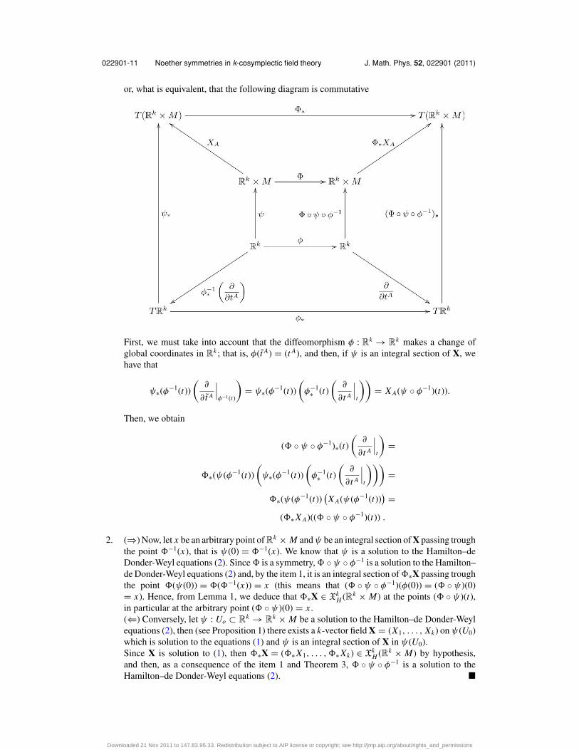
or, what is equivalent, that the following diagram is commutative
First, we must take into account that the diffeomorphism φ : Rk → Rk makes a change ofglobal coordinates in Rk ; that is, φ(t A) = (t A), and then, if ψ is an integral section of X, wehave that
ψ∗(φ−1(t))
(∂
∂ t A
∣∣∣φ−1(t)
)= ψ∗(φ−1(t))
(φ−1
∗ (t)
(∂
∂t A
∣∣∣t
))= X A(ψ ◦ φ−1)(t)).
Then, we obtain
(� ◦ ψ ◦ φ−1)∗(t)
(∂
∂t A
∣∣∣t
)=
�∗(ψ(φ−1(t))
(ψ∗(φ−1(t))
(φ−1
∗ (t)
(∂
∂t A
∣∣∣t
)))=
�∗(ψ(φ−1(t))(X A(ψ(φ−1(t))
) =(�∗ X A)((� ◦ ψ ◦ φ−1)(t)) .
2. (⇒) Now, let x be an arbitrary point ofRk × M and ψ be an integral section of X passing troughthe point �−1(x), that is ψ(0) = �−1(x). We know that ψ is a solution to the Hamilton–deDonder-Weyl equations (2). Since � is a symmetry, � ◦ ψ ◦ φ−1 is a solution to the Hamilton–de Donder-Weyl equations (2) and, by the item 1, it is an integral section of �∗X passing troughthe point �(ψ(0)) = �(�−1(x)) = x (this means that (� ◦ ψ ◦ φ−1)(φ(0)) = (� ◦ ψ)(0)= x). Hence, from Lemma 1, we deduce that �∗X ∈ Xk
H (Rk × M) at the points (� ◦ ψ)(t),in particular at the arbitrary point (� ◦ ψ)(0) = x .(⇐) Conversely, let ψ : Uo ⊂ Rk → Rk × M be a solution to the Hamilton–de Donder-Weylequations (2), then (see Proposition 1) there exists a k-vector field X = (X1, . . . , Xk) on ψ(U0)which is solution to the equations (1) and ψ is an integral section of X in ψ(U0).Since X is solution to (1), then �∗X = (�∗ X1, . . . , �∗ Xk) ∈ Xk
H (Rk × M) by hypothesis,and then, as a consequence of the item 1 and Theorem 3, � ◦ ψ ◦ φ−1 is a solution to theHamilton–de Donder-Weyl equations (2). �
Downloaded 21 Nov 2011 to 147.83.95.33. Redistribution subject to AIP license or copyright; see http://jmp.aip.org/about/rights_and_permissions

022901-12 Marrero et al. J. Math. Phys. 52, 022901 (2011)
As a consequence of this, if � is a symmetry and X is an integrable k-vector field in XkH (Rk × M),
we have that �∗X − X ∈ ker ω� ∩ ker η�.
Proposition 6: Let (Rk × M, H ) be a k-cosymplectic Hamiltonian system. If Y ∈ X(Rk × M) isan infinitesimal symmetry, then for every integrable k-vector field X = (X1, . . . , Xk) ∈ Xk
H (Rk × M)we have that [Y, X] = ([Y, X1], . . . , [Y, Xk]) ∈ ker ω� ∩ ker η�.
Proof: Denote by Ft the local 1-parameter groups of diffeomorphisms generated by Y . As Yis an infinitesimal symmetry, as a consequence of Proposition 5, we have Ft∗X − X = Z ∈ ker ω�
∩ ker η�. Then, taking a local basis of sections {Z1, . . . , Zr } = {(Z11, . . . , Z1
k ), . . . , (Zr1, . . . , Zr
k )}of the vector bundle ker ω� ∩ ker η� → Rk × M , we have that Ft∗X − X = gαZα , α = 1, . . . , r ,with gα : R × (Rk × M) → R (they are functions that depend on t , some of them different from 0);that is,
Ft∗X − X = (Ft∗ X1 − X1, . . . , Ft∗ Xk − Xk)
= (gα Zα1 , . . . , gα Zα
k ) = gαZα .
Therefore,
[Y, X] = L(Y )X = (L(Y )X1, . . . L(Y )Xk)
=(
limt→0
Ft∗ X1 − X1
t, . . . , lim
t→0
Ft∗ Xk − Xk
t
)
=(
limt→0
gα
tZα
1 , . . . , limt→0
gα
tZα
k
)
= ( fα Zα1 , . . . , fα Zα
k ) = fαZα ∈ ker ω� ∩ ker η� ,
where fα : Rk × M → R. �
B. k-cosymplectic Noether symmetries. Noether’s theorem
As it is well known, the existence of symmetries is associated with the existence of conservationlaws. How to obtain these conservation laws depends on the symmetries that we are considering.In particular, for Hamiltonian and Lagrangian systems, Noether‘s theorem gives a rule for doingit, for certain kinds of symmetries: those that preserve both the physical information (given bythe Hamiltonian or the Lagrangian function), and some geometric structures of the system. Fork-cosymplectic Hamiltonian field theories a reasonable choice consists in taking those symmetriespreserving the k-cosymplectic structure as well as the Hamiltonian function. Bearing this in mind,first we prove the following:
Proposition 7: Let (Rk × M, H ) be a k-cosymplectic Hamiltonian system.
1. If � : Rk × M −→ Rk × M is a diffeomorphism satisfying that
(a) �∗ωA = ωA,(b) �∗ηA = ηA,(c) �∗ H = H ,
then � is a symmetry of the k-cosymplectic Hamiltonian system (Rk × M, H ).(1) If Y ∈ X(Rk × M) a vector field satisfying that
(a) L(Y )ωA = 0,(b) L(Y )ηA = 0,(c) L(Y )H = 0,
then Y is an infinitesimal symmetry of the k-cosymplectic Hamiltonian system (Rk × M, H ).
Downloaded 21 Nov 2011 to 147.83.95.33. Redistribution subject to AIP license or copyright; see http://jmp.aip.org/about/rights_and_permissions

022901-13 Noether symmetries in k-cosymplectic field theory J. Math. Phys. 52, 022901 (2011)
Proof:
1. First, from
dt A = ηA = �∗ηA = �∗dt A = d�∗t A
we conclude that �∗t A = t A + k A (k A ∈ R). This result (together with the condition �∗ωA
= ωA) means that the local expression of � is �(t A, qi , pi ) = (t A + k A,�i (q, p),�Ai (q, p)).
Therefore it induces a diffeomorphism φ : Rk → Rk given by φ(t A) = t A + k A; henceπRk ◦ � = φ ◦ πRk and � is a fiber preserving map for the trivial bundle πRk : Rk × M → Rk .
Now, as ηA(RB) = dt A
(∂
∂t B
)= δA
B , and �∗ηA = �∗dt A = dt A = ηA, we have
δAB = dt A
(∂
∂t B
)= (�∗dt A)
(∂
∂t B
)= �∗
{dt A
(�∗
(∂
∂t B
))},
thus
�∗
(∂
∂t B
)= ∂
∂t B+ αi ∂
∂qi+ β A
i
∂
∂ pAi
,
but, since �∗ωA = ωA, for all A,
0 = i
(∂
∂t B
)ωA = i
(�∗
(∂
∂t B
))(ωA ◦ �)
and then
∂
∂t B+ αi ∂
∂qi+ β A
i
∂
∂pAi
= �∗
(∂
∂t B
)∈ ∩k
A=1 ker(ωA ◦ �) =⟨
∂
∂t A◦ �
⟩A=1,...,k
,
which implies that �∗
(∂
∂t B
)= ∂
∂t Bthat is, �∗(RB) = RB .
Furthermore, for every k-vector field X = (X1, . . . , Xk) ∈ XkH (Rk × M), we obtain that
�∗(ηA(�∗ X B)) = (�∗ηA)(X B) = ηA(X B) = δAB ,
�∗[
k∑A=1
i(�∗ X A)ωA − dH + (L(RA)H )ηA
]
=k∑
A=1
[i(X A)(�∗ωA) − �∗dH + (�∗ L(RA)H )(�∗ηA)
]
=k∑
A=1
[i(X A)ωA − dH + (L(RA)H )ηA] = 0 .
Hence, as � is a diffeomorphism, these results are equivalent to demanding that
ηA(�∗ X B) = δAB
k∑A=1
[i(�∗ X A)ωA − dH + L(RA)HηA] = 0 .
Thus �∗X = (�∗ X1, . . . , �∗ Xk) ∈ XkH (Rk × M). Finally, if X is integrable, then �∗X is
integrable too (as Proposition 5 claims), and thus � is a symmetry.2. It is a consequence of the above item, taking the local flows of Y .
�
Downloaded 21 Nov 2011 to 147.83.95.33. Redistribution subject to AIP license or copyright; see http://jmp.aip.org/about/rights_and_permissions

022901-14 Marrero et al. J. Math. Phys. 52, 022901 (2011)
Although the condition 2(b) of the hypothesis is sufficient to prove that these kinds of vectorfields are infinitesimal symmetries, in order to achieve a good generalization of Noether’s theo-rem, this condition must be hardened by demanding that i(Y )ηA = 0 [observe that i(Y )dt A = 0=⇒ L(Y )dt A = 0]. This is equivalent to write L(Y )t A = 0 and hence, the equivalent global condi-tion 1(b) for this case is �∗t A = t A. This means that the induced diffeormorphism φ : Rk → Rk isthe identity on Rk .
Taking into account all of this, we introduce the following definitions:
Definition 10: Let (Rk × M, H ) be a k-cosymplectic Hamiltonian system.
1. A k-cosymplectic Noether symmetry is a diffeomorphism � : Rk × M −→ Rk × M satisfyingthe following conditions:
(a) �∗ωA = ωA,(b) �∗t A = t A,(c) �∗ H = H .
If the k-symplectic structure is exact, a k-cosymplectic Noether symmetry is said to be exact if�∗θ A = θ A.In the particular case that M = (T 1
k )∗Q (the standard model), if � = j1∗ϕ for some diffeo-morphism ϕ : Rk × Q −→ Rk × Q, then the k-cosymplectic Noether symmetry � is said tobe natural.
2. Let (Rk × M, H ) be a k-cosymplectic Hamiltonian system. An infinitesimal k-cosymplecticNoether symmetry is a vector field Y ∈ X(Rk × M) whose local flows are local k-cosymplecticNoether symmetries; that is, it satisfies that:
(a) L(Y )ωA = 0,(b) i(Y )ηA = 0,(c) L(Y )H = 0.
If the k-symplectic structure is exact, an infinitesimal k-cosymplectic Noether symmetry is saidto be exact if L(Y )θ A = 0.In the particular case that M = (T 1
k )∗ Q, if Y = Z1∗ for some Z ∈ X(Rk × Q), then theinfinitesimal k-cosymplectic Noether symmetry Y is said to be natural.
[Obviously natural (infinitesimal) k-cosymplectic Noether symmetries are exact].
Lemma 2: If Y ∈ X(Rk × M) is an infinitesimal k-cosymplectic Noether symmetry, then[Y, RA] = 0.
Proof: In fact, for all A, B, we have that
i([Y, RA])ωB = L(Y ) i(RA)ωB − i(RA) L(Y )ωB = 0 =⇒ [Y, RA] ∈ ker ωB,
i([Y, RA])ηB = L(Y ) i(RA)ηB − i(RA) L(Y )ηB = L(Y )δBA = 0 =⇒ [Y, RA] ∈ ker ηB,
and then [Y, RA] ∈ (∩B ker ωB) ∩ (∩B ker ηB) = {0}. �Remarks:
� The condition �∗t A = t A means that k-cosymplectic Noether symmetries generate transforma-tions along the fibers of the projection πRk : Rk × M −→ Rk ; that is, they leave the fibers ofthe projection πRk : Rk × M −→ Rk invariant or, what means the same thing, πRk ◦ � = πRk .As a consequence, in the particular case that M = (T 1
k )∗Q, if � = j1∗ϕ (for some diffeo-morphism ϕ : Rk × Q −→ Rk × Q) is a natural k-cosymplectic Noether symmetry, thenthe diffeomorphism ϕ : Rk × Q −→ Rk × Q must leave the fibers of the projection pRk :Rk × Q −→ Rk invariant necessarily; that is, pRk ◦ ϕ = pRk .
� In the case of infinitesimal k-cosymplectic Noether symmetries the analogous condition is
i(Y )dt A = 0, which means that Y has the local expression Y = Yi∂
∂qi+ Y A
i
∂
∂pAi
. This means
Downloaded 21 Nov 2011 to 147.83.95.33. Redistribution subject to AIP license or copyright; see http://jmp.aip.org/about/rights_and_permissions

022901-15 Noether symmetries in k-cosymplectic field theory J. Math. Phys. 52, 022901 (2011)
that Y is tangent to the fibers of the projection πRk : Rk × M −→ Rk . Thus these infinitesimalsymmetries only generate transformations along these fibers, or, what means the same thing,the local flows of the generators Y leave the fibers of the projection πRk : Rk × M −→ Rk
invariant. Furthermore, as a consequence of the above Lemma and taking into account that
RA = ∂
∂t A, in this local expression for Y the component functions Yi , Y A
i do not depend on
the coordinates (t A).Observe also that, in the particular case that M = (T 1
k )∗Q, if Y = Z1∗ [for some Z ∈ X(Rk
× Q)] is a natural infinitesimal k-cosymplectic Noether symmetry, then i(Y )dt A = 0, neces-sarily.
In addition, it is immediate to prove that, if Y1, Y2 ∈ X(Rk × M) are infinitesimal Noethersymmetries, then so is [Y1, Y2].
It is interesting to comment that, for infinitesimal k-cosymplectic Noether symmetries, theresults in the item 2 of Proposition 5 and in Proposition 6 hold, not only for integrable k-vectorfields in Xk
H (Rk × M), but also for every k-vector field X ∈ XkH (Rk × M). In fact, for the first one,
we havek∑
A=1
i([Y, X A])ωA =k∑
A=1
{L(Y ) i(X A)ωA − i(X A) L(Y )ωA}
=k∑
A=1
L(Y )(dH − (L(RA)H )ηA)
=k∑
A=1
{d(L(Y )(H )) − (L(Y ) L(RA)H )ηA
−(L(RA)H ) L(Y )ηA}
= −k∑
A=1
(L(RA) L(Y )H )ηA = 0 .
Furthermore,
i([Y, X A])ηB = L(Y ) i(X A)ηB − i(X A) L(Y )ηB = 0 ,
and the proof for the second one is straightforward.As infinitesimal k-cosymplectic Noether symmetries are vector fields in Rk × M whose local
flows are local k-cosymplectic Noether symmetries, all the results that we state for k-cosymplecticNoether symmetries also hold for infinitesimal k-cosymplectic Noether symmetries. Hence, fromnow on we consider only the infinitesimal case.
A first relevant result is the following:
Proposition 8: Let Y ∈ X(Rk × M) be an infinitesimal k-cosymplectic Noether symmetry. Then,for every p ∈ Rk × M, there is an open neighborhood Up � p, such that:
1. There exist F A ∈ C∞(Up), which are unique up to constant functions, such that
i(Y )ωA = dF A, (on Up) . (10)
2. There exist ζ A ∈ C∞(Up), verifying that L(Y )θ A = dζ A, on Up; and then
F A = i(Y )θ A − ζ A , (up to a constant function, on Up) .
Proof:
1. It is a consequence of the Poincare Lemma and the condition
0 = L(Y )ωA = i(Y )dωA + d i(Y )ωA = d i(Y )ωA .
Downloaded 21 Nov 2011 to 147.83.95.33. Redistribution subject to AIP license or copyright; see http://jmp.aip.org/about/rights_and_permissions
022901-16 Marrero et al. J. Math. Phys. 52, 022901 (2011)
2. We have that
d L(Y )θ A = L(Y )dθ A = − L(Y )ωA = 0
and hence L(Y )θ A are closed forms. Therefore, by the Poincare Lemma, there exist ζ A ∈C∞(Up), verifying that L(Y )θ A = dζ A, on Up. Furthermore, as (10) holds on Up, we obtainthat
dζ A = L(Y )θ A = d i(Y )θ A + i(Y )dθ A
= d i(Y )θ A − i(Y )ωA = d{i(Y )θ A − F A} ,
and thus 2 holds. �
Remark: For exact infinitesimal k-cosymplectic Noether symmetries we have thatF A = i(Y )θ A
(up to a constant function).Finally, the classical Noether’s theorem can be stated for these kinds of symmetries as follows:
Theorem 4: (Noether’s theorem). If Y ∈ X(Rk × M) is an infinitesimal k-cosymplectic Noethersymmetry then, for every p ∈ Rk × M, there is an open neighborhood Up � p such that the functionsF A = i(Y )θ A − ζ A, define a conservation law F = (F1, . . . ,F k).
Proof: Let X = (X1, . . . , Xk) ∈ XkH (Rk × M) an integrable k-vector field. From (10), one ob-
tainsk∑
A=1
L(X A)F A =k∑
A=1
i(X A)dF A =k∑
A=1
i(X A) i(Y )ωA
= − i(Y )k∑
A=1
i(X A)ωA
= − i(Y )dH +k∑
A=1
i(Y )((L(RA)H )ηA)
= − L(Y )H +k∑
A=1
(L(RA)H ) i(Y )ηA = 0 ,
that is, F = (F1, . . . ,F k) is a conservation law for the Hamilton–de Donder-Weyl equations. �Observe that, using Darboux coordinates in Rk × M , the item 2 of Proposition 8 tells us that
the conservation laws associated with infinitesimal k-cosymplectic Noether symmetries does notdepend on the coordinates (t A) (as it is obvious since the generators of these symmetries, the vectorfields Y , neither depend on them).
IV. EXAMPLE
A. k-cosymplectic quadratic Hamiltonian systems
Many Hamiltonian systems in field theories are of “quadratic” type and they can be modeled asfollows.
Consider the k-cosymplectic manifold (Rk × (T 1k )∗ Q, ηA, ωA,V). Let g1, . . . , gk be k semi-
Riemannian metrics in Q. For every q ∈ Q we have the following isomorphisms:
g�
A : Tq Q −→ T ∗q Q
v �→ i(v)gA,
with A ∈ {1, . . . , k} and then we can introduce the dual metric of gA, denoted by g∗A, which is
defined by
g∗A(αq , βq ) := gA((g�
A)−1(αq ), (g�
A)−1(βq )) ,
Downloaded 21 Nov 2011 to 147.83.95.33. Redistribution subject to AIP license or copyright; see http://jmp.aip.org/about/rights_and_permissions

022901-17 Noether symmetries in k-cosymplectic field theory J. Math. Phys. 52, 022901 (2011)
for every αq , βq ∈ T ∗q Q, and A ∈ {1, . . . , k}. We can define a function K ∈ C∞(Rk × (T 1
k )∗ Q) asfollows: for every (t, q; α1
q , . . . , αkq ) ∈ Rk × (T 1
k )∗Q,
K (t, q; α1q , . . . , α
kq ) := 1
2
k∑A=1
g∗A(αA
q , αAq ).
Then, if V ∈ C∞(Rk × Q) we can introduce a Hamiltonian function H ∈ C∞(Rk × (T 1k )∗ Q) of
quadratic type as follows
H = K + V ◦ (πQ)∗1,0.
Using natural coordinates (t A, qi , pAi ) on Rk × (T 1
k )∗ Q the local expression of H is
H (t A, qi , pAi ) = 1
2
k∑A=1
gi jA (qk)pA
i pAj + V (t B, q j ) ,
where gi jA denote the coefficients of the matrix associated to g∗
A. Then
dH =k∑
A=1
[∂V
∂t Adt A +
(1
2
∂gi jA
∂qkpA
i pAj + ∂V
∂qk
)dqk + (gi j
A pAi )dpA
j
]
Moreover, if X = (X1, . . . , Xk) ∈ XkH (Rk × (T 1
k )∗ Q) with
X A =k∑
B=1
[(X A)B ∂
∂t B + (X A)i ∂
∂qi + (X A)Bi
∂
∂pBi
]
the equations (1) lead to
(X A)B = δBA , (X A)i = gi j
A pAj (A fixed) ,
−k∑
A=1
(X A)Ai = 1
2
k∑A=1
∂g jkA
∂qipA
j pAk + ∂V
∂qi; (11)
that is, we have obtained
X A =[
∂
∂t A+ gi j
A pAj
∂
∂qi+ (X A)B
i
∂
∂ pBi
],
with (X B)Bi = − ∂V
∂qi− 1
2
∂g jkA
∂qipA
j pAk .
Now, if ψ(t) = (t A, ψ i (t), ψ Ai (t)) is an integral section of X then
X A(ψ(t)) = ψ∗(t)
(∂
∂t A
∣∣∣t
)=
[∂
∂t A+ ∂ψ i
∂t A
∂
∂qi+ ∂ψ B
i
∂t A
∂
∂ pBi
]. (12)
Thus, from (11) and (12), we obtain the Hamilton–de Donder-Weyl equations
− ∂V
∂qi(ψ(t)) − 1
2
∂gi jA
∂qiψ A
j ψ Ak =
k∑A=1
(X A)Ai (ψ(t)) =
k∑A=1
∂ψ Ai
∂t A
gi jA (ψ(t))ψ A
j = X Ai (ψ(t)) = ∂ψ i
∂t A(A, i fixed) . (13)
Then, from these equations we conclude that
ψ Ai = (gA)i j
∂ψ j
∂t A(A, i fixed) ,
Downloaded 21 Nov 2011 to 147.83.95.33. Redistribution subject to AIP license or copyright; see http://jmp.aip.org/about/rights_and_permissions

022901-18 Marrero et al. J. Math. Phys. 52, 022901 (2011)
and hence the equations for the integral sections are
∑A, j
(gA)i j∂2ψ j
∂(t A)2= − ∂V
∂qi− 1
2
∑A, j,k,l,m
∂g jkA
∂qi(gA)kl(gA) jm
∂ψ l
∂t A
∂ψm
∂t A. (14)
We also may prove the following result:
Proposition 9: Let X be a Killing vector field on Q for the semi-Riemannian metrics g1, . . . , gk
(that is, L(X )gA = 0, for all A ∈ {1, . . . , k}) such that X (V ) = 0. Then, the vector field X1∗ onRk × (T 1
k )∗ Q is a natural infinitesimal symmetry for the k-cosymplectic Hamiltonian system (Rk
× (T 1k )∗ Q, H ). Thus, if F = (X , . . . , X ) : Rk × (T 1
k )∗Q → Rk is the map defined by
F(t, q; α1q , . . . , α
kq ) = (α1
q (X (q)), . . . , αkq (X (q))),
for (t, q; α1q , . . . , α
kq ) ∈ Rk × (T 1
k )∗ Q, we have that F is a conservation law for the Hamiltoniansystem.
Proof: As we know
L(X1∗)θ A = 0.
Moreover, it is clear that
i(X1∗)ηA = 0.
So, it is sufficient to prove that
L(X1∗)H = 0.
Now, using that X1∗ is (πQ)∗1,0-projectable over X and the fact that L(X )V = 0, we deduce that
L(X1∗)(V ◦ (πQ)∗1,0) = 0 .
Next, we will prove that
L(X1∗)(K ) = 0 .
Assuming that the local expression of X is
X = Xi ∂
∂qi,
then, as L(X )gA = 0, we have that
X ((gA) jk) = −∂ Xl
∂q j(gA)kl − ∂ Xl
∂qk(gA) jl ,
which implies that
X (gi jA ) = −∂ X j
∂qkgik
A − ∂ Xi
∂qkg jk
A .
Therefore, using that the local expressions of X1∗ and K are
X1∗ = Xi ∂
∂qi− pA
j
∂ X j
∂qi
∂
∂pAi
, K = 1
2
∑A,i, j
gi jA pA
i pAj
we conclude that
L(X1∗)K = 0 .
Furthermore, if X : T ∗ Q → R is the linear function on T ∗ Q associated with the vector field X , itfollows that
(i(X1∗)θ A)(t, q; α1q , . . . , α
kq ) = X (αA
q ) .
Consequently, F = (X , . . . , X ) is a conservation law (see Remark after Proposition 8). �
Downloaded 21 Nov 2011 to 147.83.95.33. Redistribution subject to AIP license or copyright; see http://jmp.aip.org/about/rights_and_permissions

022901-19 Noether symmetries in k-cosymplectic field theory J. Math. Phys. 52, 022901 (2011)
B. A particular case: The wave equation
As particular examples of these kinds of systems we can detach the following case (see Ref. 24for a more detailed explanation):
Consider the three-dimensional wave equation,
σ∂2ψ
∂t2 − τ
(∂2ψ
∂x2 + ∂2ψ
∂y2 + ∂2ψ
∂z2
)= 0 . (15)
In this case M = R4 × (T 12 )∗Q (i.e., k = 4), with Q = R (n = 1), and gi , i = 1, . . . , 4, are the
semi-Riemannian metrics on R,
g1 = σdq2, g2 = g3 = g4 = −τdq2,
q being the standard coordinate on R. We have done the identifications t1 ≡ t and t2 ≡ x, t3
≡ y, t4 ≡ z, where t is time and x, y, z denote the position in space. Then, ψ(t, x, y, z) denotes thedisplacement of each point of the media where the wave is propagating, as function of the time andthe position, and σ and τ are physical constants.
Thus, the wave equation (15) is a particular case of the equation (14) for the quadratic Hamil-tonian in R2 × (T 1
2 )∗R
H = 1
2
[1
σ(p1)2 − 1
τ
((p2)2 + (p3)2 + (p4)2
)].
We have that the canonical vector field,∂
∂qon R is a Killing vector field for the semi-Riemannian
metrics gi , i = 1, . . . , 4. Thus,
F = (p1, p2, p3, p4) : R4 × (T 14 )∗R → R4
is a conservation law for the three-dimensional wave equation.Note that if
ψ : (t, x, y, z) → (t, x, y, z, ψ(t, x, y, z);
ψ1(t, x, y, z), ψ2(t, x, y, z), ψ3(t, x, y, z), ψ4(t, x, y, z))
is a solution to the Hamilton–de Donder-Weyl equations then, from (14), it follows that
ψ1 = σ∂ψ
∂t, ψ2 = −τ
∂ψ
∂x, ψ3 = −τ
∂ψ
∂y, ψ4 = −τ
∂ψ
∂z.
Thus, the conservation law leads to the starting field equations. In fact,
Div(F ◦ ψ) = σ∂2ψ
∂t2 − τ
(∂2ψ
∂x2 + ∂2ψ
∂y2 + ∂2ψ
∂z2
)= 0.
V. CONCLUSIONS AND OUTLOOK
We have studied symmetries and reduction of k-cosymplectic Hamiltonian systems in classi-cal field theories; in particular, those which are modeled on k-cosymplectic manifolds M = Rk
× M , with M being a generic k-symplectic manifold (which we have called almost-standard k-cosymplectic manifolds).
In particular, we have analyzed a kind of k-cosymplectic Noether symmetries for which thereis a direct way to associate conservation laws by means of the application of the correspondinggeneralized version of the Noether theorem.
As discussed in Sec. III, for the almost-standard k-cosymplectic Hamiltonian systems, thesymmetries that we have considered in this work have the following geometric characteristic: theygenerate transformations along the fibers of the projection Rk × M −→ Rk . As a consequence, in alocal description, the associated conservation laws do not depend on the base coordinates (t A). Thiscould seem to be a strong restriction but, really, many symmetries of field theories in physics are of
Downloaded 21 Nov 2011 to 147.83.95.33. Redistribution subject to AIP license or copyright; see http://jmp.aip.org/about/rights_and_permissions

022901-20 Marrero et al. J. Math. Phys. 52, 022901 (2011)
this type. In any case, a theory of symmetries, conservation laws, and reduction concerning to moregeneral kinds of symmetries would have to be developed.
ACKNOWLEDGMENTS
We acknowledge the partial financial support of the Ministerio de Ciencia e Innovacion (Spain),projects MTM2008-00689, MTM2009-13383, and MTM2009-08166-E. We thank the referee forhis valuable suggestions and comments which have allowed us to significantly improve some partsof this work.
1 Albert, C., “Le theoreme de reduction de Marsden-Weinstein en geometrie cosymplectique et de contact,” J. Geom. Phys.6(4), 627 (1989).
2 Awane, A., “k-symplectic structures,” J. Math. Phys. 33, 4046 (1992).3 Awane, A., “G-spaces k-symplectic homogenes,” J. Geom. Phys. 13, 139 (1994).4 Awane, A. and Goze, M., Pfaffian systems, k-symplectic systems (Kluwer Academic Publishers , Dordrecht, 2000).5 Castrillon-Lopez, M. and Marsden, J. E., “Some remarks on Lagrangian and Poisson reduction for field theories,” J. Geom.
Phys. 48(1), 52 (2003).6 de Leon, M. and de Diego, D. M., “Symmetries and constant of the motion for singular Lagrangian systems,” Int. J. Theor.
Phys. 35(5), 975, (1996).7 de Leon, M., de Diego, D. M., and Santamarıa-Merino, A.,“Symmetries in classical field theories,” Int. J. Geom. Meth.
Mod. Phys. 1(5), 651 (2004).8 de Leon, M., Mendez, I., and Salgado, M., “p-almost cotangent structures,” Boll. Uni. Mat. Ital. A 7(7), 97
(1993).9 de Leon, M., Merino, E., Oubina, J. A., Rodrigues, P., and Salgado, M., “Hamiltonian systems on k-cosymplectic
manifolds,” J. Math. Phys. 39(2), 876 (1998).10 de Leon, M., Merino, E., and Salgado, M., “k-cosymplectic manifolds and Lagrangian field theories,” J. Math. Phys.
42(5), 2092 (2001).11 Dieudonne, J., Foundations of Modern Analysis. Pure and Applied Mathematics, Vol. 10-I (Academic Press, New York,
1969), p. 387.12 Echeverrıa-Enrıquez, A., Munoz-Lecanda, M. C., and Roman-Roy, N., “Multivector field formulation of Hamiltonian
field theories: Equations and symmetries,” J. Phys. A 32(48), 8461 (1999).13 Giachetta, G., Mangiarotti, L., and Sardanashvily, G., New Lagrangian and Hamiltonian Methods in Field Theory (World
Scientific, Singapore, 1997).14 Gotay, M. J., “A multisymplectic framework for classical field theory and the calculus of variations, I. Covariant Hamil-
tonian formalism,” in Mechanics, Analysis and Geometry: 200 Years After Lagrange (North-Holland, Amsterdam, 1991),pp. 203–235.
15 Gotay, M., Isenberg, J., and Marsden, J. E., “Momentum maps and classical relativistic fields, Part I: Covariant field theory,”e-print www.arxiv.org: [2004] physics/9801019; “Part II: Canonical analysis of field theories,” e-print ww.arxiv.org: [2004]math-ph/0411032.
16 Gunther, C., “The polysymplectic Hamiltonian formalism in field theory and calculus of variations. I: The local case,” J.Differ. Geom. 25, 23 (1987).
17 Kanatchikov, I. V., “Canonical structure of classical field theory in the polymomentum phase space,” Rep. Math. Phys.41(1), 49, (1998).
18 Kijowski, J., “A finite-dimensional canonical formalism in the classical field theory,” Comm. Math. Phys. 30, 99 (1973).19 Kijowski, J. and Tulczyjew, W. M., A symplectic framework for field theories, Lecture Notes in Physics Vol. 107 (Springer-
Verlag, New York, 1979).20 Kolar, I., Michor, P., and Slovak, J., Natural Operations in Differential Geometry (Springer-Verlag, Berlin, 1993).21 Lee, J. M., Introduction to Smooth Manifolds (Springer, New York, 2003).22 McLean, M. and Norris, L. K., “Covariant field theory on frame bundles of fibered manifolds,” J. Math. Phys. 41(10),
6808 (2000).23 Munteanu, F., Rey, A. M., and Salgado, M., “The Gunther’s formalism in classical field theory: Momentum map and
reduction,” J. Math. Phys. 45(5), 1730 (2004).24 Munoz-Lecanda, M. C., Salgado, M., and Vilarino, S., “k-symplectic and k-cosymplectic Lagrangian field theories: Some
interesting examples and applications,”, Int. J. Geom. Meth. Mod. Phys. 7(4), 669 (2010).25 Norris, L. K., “Generalized symplectic geometry on the frame bundle of a manifold,” Proc. Symp. Pure Math. 54, (Part 2)
(American Mathematical Society, Providence, 1993), pp. 435–465.26 Norris, L. K., “n-symplectic algebra of observables in covariant Lagrangian field theory,” J. Math. Phys. 42(10), 4827
(2001).27 Olver, P. J., Applications of Lie Groups to Differential Equations, Graduate Texts in Mathematics Vol. 107 (Springer-Verlag,
New York, 1986).28 Roman-Roy, N., Salgado, M., and Vilarino, S., “Symmetries and conservation laws in the Gunther k-symplectic formalism
of field theory,” Rev. Math. Phys. 19(10), 1117 (2007).29 Sardanashvily, G., Generalized Hamiltonian Formalism for Field Theory. Constraint Systems (World Scientific, Singapore,
1995).
Downloaded 21 Nov 2011 to 147.83.95.33. Redistribution subject to AIP license or copyright; see http://jmp.aip.org/about/rights_and_permissions