on a half-discrete hilbert-type inequality similar to mulholland’s inequality
TRANSCRIPT
Huang and Yang Journal of Inequalities and Applications 2013, 2013:290http://www.journalofinequalitiesandapplications.com/content/2013/1/290
RESEARCH Open Access
On a half-discrete Hilbert-type inequalitysimilar to Mulholland’s inequalityZhenxiao Huang1 and Bicheng Yang2*
*Correspondence:[email protected];[email protected] of Mathematics,Guangdong University ofEducation, Guangzhou, Guangdong510303, P.R. ChinaFull list of author information isavailable at the end of the article
AbstractBy using the way of weight functions and Hadamard’s inequality, a half-discreteHilbert-type inequality similar to Mulholland’s inequality with a best constant factor isgiven. The extension with multi-parameters, the equivalent forms as well as theoperator expressions are also considered.MSC: 26D15
Keywords: Hilbert-type inequality; weight function; equivalent form
1 IntroductionAssuming that f , g ∈ L(R+), ‖f ‖ = {∫ ∞
f (x)dx} > , ‖g‖ > , we have the following
Hilbert integral inequality (cf. []):
∫ ∞
∫ ∞
f (x)g(y)x + y
dxdy < π‖f ‖‖g‖, ()
where the constant factor π is the best possible. If a = {an}∞n=, b = {bn}∞n= ∈ l, ‖a‖ ={∑∞
n= an} > , ‖b‖ > , then we still have the following discrete Hilbert inequality:
∞∑m=
∞∑n=
ambnm + n
< π‖a‖‖b‖, ()
with the same best constant factor π . Inequalities () and () are important in analysisand its applications (cf. [–]). Also we have the followingMulholland inequality with thesame best constant factor (cf. [, ]):
∞∑m=
∞∑n=
ambnlnmn
< π
{ ∞∑m=
mam∞∑n=
nbn
}
. ()
In , by introducing an independent parameter λ ∈ (, ], Yang [] gave an exten-sion of (). By generalizing the results from [], Yang [] gave some best extensions of() and () as follows: If p > ,
p + q = , λ + λ = λ, kλ(x, y) is a non-negative homoge-
neous function of degree –λ with k(λ) =∫ ∞ kλ(t, )tλ– dt ∈ R+, φ(x) = xp(–λ)–, ψ(x) =
xq(–λ)–, f (≥ ) ∈ Lp,φ(R+) = {f |‖f ‖p,φ := {∫ ∞ φ(x)|f (x)|p dx}
p < ∞}, g (≥ ) ∈ Lq,ψ (R+),
© 2013 Huang and Yang; licensee Springer. This is an Open Access article distributed under the terms of the Creative CommonsAttribution License (http://creativecommons.org/licenses/by/2.0), which permits unrestricted use, distribution, and reproductionin any medium, provided the original work is properly cited.
Huang and Yang Journal of Inequalities and Applications 2013, 2013:290 Page 2 of 8http://www.journalofinequalitiesandapplications.com/content/2013/1/290
‖f ‖p,φ ,‖g‖q,ψ > , then
∫ ∞
∫ ∞
kλ(x, y)f (x)g(y)dxdy < k(λ)‖f ‖p,φ‖g‖q,ψ , ()
where the constant factor k(λ) is the best possible. Moreover, if kλ(x, y) is finite andkλ(x, y)xλ– (kλ(x, y)yλ–) is decreasing for x > (y > ), then for am,bn ≥ , a = {am}∞m= ∈lp,φ = {a|‖a‖p,φ := {∑∞
n= φ(n)|an|p}p <∞}, b = {bn}∞n= ∈ lq,ψ , ‖a‖p,φ ,‖b‖q,ψ > , we have
∞∑m=
∞∑n=
kλ(m,n)ambn < k(λ)‖a‖p,φ‖b‖q,ψ , ()
with the same best constant factor k(λ). Clearly, for p = q = , λ = , k(x, y) = x+y , λ =
λ = , () reduces to (), while () reduces to (). Some other results about Hilbert-type
inequalities are provided by [, –].On the topic of half-discrete Hilbert-type inequalities with the general non-
homogeneous kernels, Hardy et al. provided a few results in Theorem of []. But theydid not prove that the constant factors in the inequalities are the best possible. Moreover,Yang [] gave an inequality with the particular kernel
(+nx)λ and an interval variable,and proved that the constant factor is the best possible. Recently, [] and [] gave thefollowing half-discrete Hilbert inequality with the best constant factor π :
∫ ∞
f (x)
∞∑n=
an(x + n)λ
dx < π‖f ‖‖a‖. ()
In this paper, by using the way of weight functions and Hadamard’s inequality, a half-discrete Hilbert-type inequality similar to () and () with the best constant factor is givenas follows:
∫ ∞
f (x)
∞∑n=
anln e(n +
)xdx < π‖f ‖
{ ∞∑n=
(n +
)an
}
. ()
Moreover, the best extension of () with multi-parameters, some equivalent forms as wellas the operator expressions are considered.
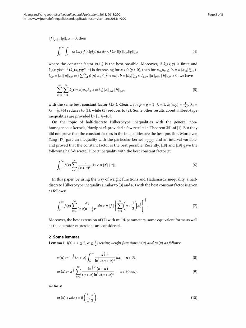
2 Some lemmasLemma If < λ ≤ , α ≥
, setting weight functions ω(n) and � (x) as follows:
ω(n) := lnλ (n + α)
∫ ∞
x λ –
lnλ e(n + α)xdx, n ∈N, ()
� (x) := x λ
∞∑n=
lnλ –(n + α)
(n + α) lnλ e(n + α)x, x ∈ (,∞), ()
we have
� (x) < ω(n) = B(
λ
,λ
). ()
Huang and Yang Journal of Inequalities and Applications 2013, 2013:290 Page 3 of 8http://www.journalofinequalitiesandapplications.com/content/2013/1/290
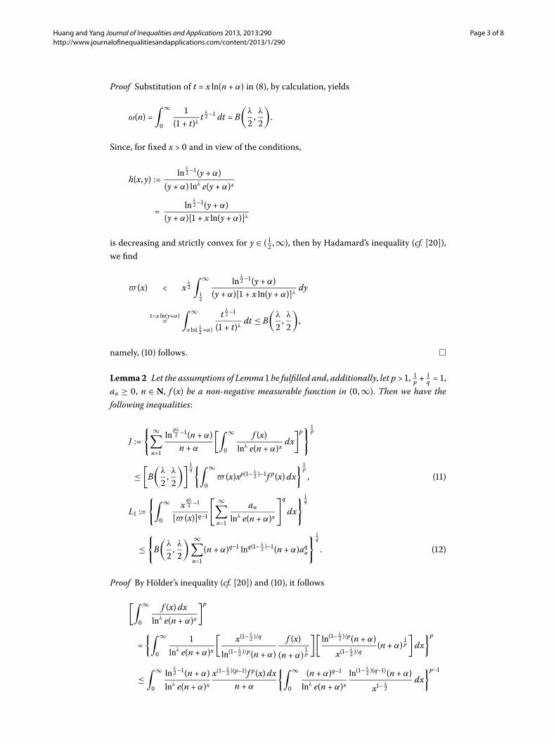
Proof Substitution of t = x ln(n + α) in (), by calculation, yields
ω(n) =∫ ∞
( + t)λ
t λ – dt = B
(λ
,λ
).
Since, for fixed x > and in view of the conditions,
h(x, y) :=ln
λ –(y + α)
(y + α) lnλ e(y + α)x
=ln
λ –(y + α)
(y + α)[ + x ln(y + α)]λ
is decreasing and strictly convex for y ∈ ( ,∞), then by Hadamard’s inequality (cf. []),we find
� (x) < x λ
∫ ∞
lnλ –(y + α)
(y + α)[ + x ln(y + α)]λdy
t=x ln(y+α)=∫ ∞
x ln( +α)
t λ –
( + t)λdt ≤ B
(λ
,λ
),
namely, () follows. �
Lemma Let the assumptions of Lemma be fulfilled and, additionally, let p > , p +q = ,
an ≥ , n ∈ N, f (x) be a non-negative measurable function in (,∞). Then we have thefollowing inequalities:
J :={ ∞∑
n=
lnpλ –(n + α)n + α
[∫ ∞
f (x)lnλ e(n + α)x
dx]p
} p
≤[B(
λ
,λ
)] q{∫ ∞
� (x)xp(– λ
)–f p(x)dx}
p, ()
L :={∫ ∞
xqλ –
[� (x)]q–
[ ∞∑n=
anlnλ e(n + α)x
]q
dx}
q
≤{B(
λ
,λ
) ∞∑n=
(n + α)q– lnq(–λ )–(n + α)aqn
} q
. ()
Proof By Hölder’s inequality (cf. []) and (), it follows
[∫ ∞
f (x)dxlnλ e(n + α)x
]p
={∫ ∞
lnλ e(n + α)x
[x(– λ
)/q
ln(–λ )/p(n + α)
f (x)
(n + α)p
][ln(–
λ )/p(n + α)x(– λ
)/q(n + α)
p
]dx
}p
≤∫ ∞
lnλ –(n + α)
lnλ e(n + α)xx(– λ
)(p–)f p(x)dxn + α
{∫ ∞
(n + α)q–
lnλ e(n + α)xln(–
λ )(q–)(n + α)x– λ
dx
}p–
Huang and Yang Journal of Inequalities and Applications 2013, 2013:290 Page 4 of 8http://www.journalofinequalitiesandapplications.com/content/2013/1/290
={
ω(n)(n + α)q–
lnq(λ –)+(n + α)
}p– ∫ ∞
lnλ –(n + α)
lnλ e(n + α)xx(– λ
)(p–)f p(x)dxn + α
=[B(
λ
,λ
)]p– n + α
lnpλ –(n + α)
∫ ∞
lnλ –(n + α)
lnλ e(n + α)xx(– λ
)(p–)f p(x)dxn + α
.
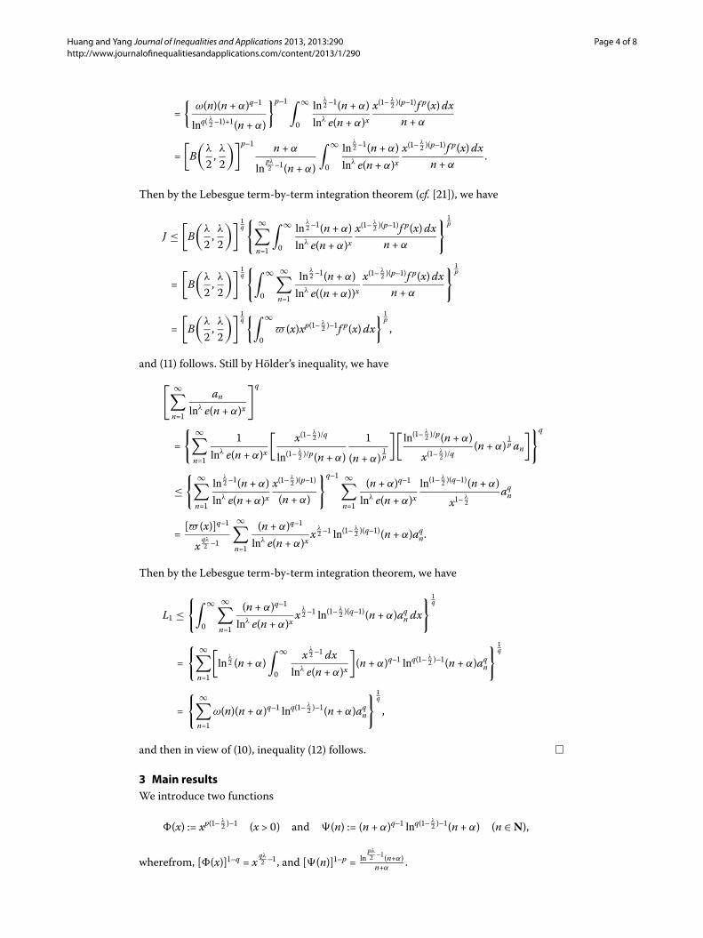
Then by the Lebesgue term-by-term integration theorem (cf. []), we have
J ≤[B(
λ
,λ
)] q{ ∞∑
n=
∫ ∞
lnλ –(n + α)
lnλ e(n + α)xx(– λ
)(p–)f p(x)dxn + α
} p
=[B(
λ
,λ
)] q{∫ ∞
∞∑n=
lnλ –(n + α)
lnλ e((n + α))xx(– λ
)(p–)f p(x)dxn + α
} p
=[B(
λ
,λ
)] q{∫ ∞
� (x)xp(– λ
)–f p(x)dx}
p,
and () follows. Still by Hölder’s inequality, we have[ ∞∑n=
anlnλ e(n + α)x
]q
={ ∞∑
n=
lnλ e(n + α)x
[x(– λ
)/q
ln(–λ )/p(n + α)
(n + α)p
][ln(–
λ )/p(n + α)x(– λ
)/q(n + α)
p an
]}q
≤{ ∞∑
n=
lnλ –(n + α)
lnλ e(n + α)xx(– λ
)(p–)
(n + α)
}q– ∞∑n=
(n + α)q–
lnλ e(n + α)xln(–
λ )(q–)(n + α)x– λ
aqn
=[� (x)]q–
xqλ –
∞∑n=
(n + α)q–
lnλ e(n + α)xx λ
– ln(–λ )(q–)(n + α)aqn.
Then by the Lebesgue term-by-term integration theorem, we have
L ≤{∫ ∞
∞∑n=
(n + α)q–
lnλ e(n + α)xx λ
– ln(–λ )(q–)(n + α)aqn dx
} q
={ ∞∑
n=
[ln
λ (n + α)
∫ ∞
x λ – dx
lnλ e(n + α)x
](n + α)q– lnq(–
λ )–(n + α)aqn
} q
={ ∞∑
n=ω(n)(n + α)q– lnq(–
λ )–(n + α)aqn
} q
,
and then in view of (), inequality () follows. �
3 Main resultsWe introduce two functions
(x) := xp(– λ )– (x > ) and (n) := (n + α)q– lnq(–
λ )–(n + α) (n ∈N),
wherefrom, [(x)]–q = xqλ –, and [(n)]–p = ln
pλ –(n+α)n+α
.
Huang and Yang Journal of Inequalities and Applications 2013, 2013:290 Page 5 of 8http://www.journalofinequalitiesandapplications.com/content/2013/1/290
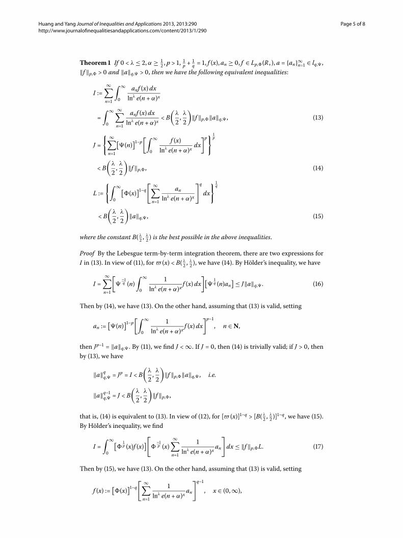
Theorem If < λ ≤ , α ≥ , p > ,
p +
q = , f (x),an ≥ , f ∈ Lp,(R+), a = {an}∞n= ∈ lq, ,
‖f ‖p, > and ‖a‖q, > , then we have the following equivalent inequalities:
I :=∞∑n=
∫ ∞
anf (x)dxlnλ e(n + α)x
=∫ ∞
∞∑n=
anf (x)dxlnλ e(n + α)x
< B(
λ
,λ
)‖f ‖p,‖a‖q, , ()
J ={ ∞∑
n=
[(n)
]–p[∫ ∞
f (x)lnλ e(n + α)x
dx]p
} p
< B(
λ
,λ
)‖f ‖p,, ()
L :={∫ ∞
[(x)
]–q[ ∞∑n=
anlnλ e(n + α)x
]q
dx}
q
< B(
λ
,λ
)‖a‖q, , ()
where the constant B( λ ,
λ ) is the best possible in the above inequalities.
Proof By the Lebesgue term-by-term integration theorem, there are two expressions forI in (). In view of (), for � (x) < B( λ
,λ ), we have (). By Hölder’s inequality, we have
I =∞∑n=
[
–q (n)
∫ ∞
lnλ e(n + α)x
f (x)dx][
q (n)an
] ≤ J‖a‖q, . ()
Then by (), we have (). On the other hand, assuming that () is valid, setting
an :=[(n)
]–p[∫ ∞
lnλ e(n + α)x
f (x)dx]p–
, n ∈N,
then Jp– = ‖a‖q, . By (), we find J < ∞. If J = , then () is trivially valid; if J > , thenby (), we have
‖a‖qq, = Jp = I < B(
λ
,λ
)‖f ‖p,‖a‖q, , i.e.
‖a‖q–q, = J < B(
λ
,λ
)‖f ‖p,,
that is, () is equivalent to (). In view of (), for [� (x)]–q > [B( λ ,
λ )]
–q, we have ().By Hölder’s inequality, we find
I =∫ ∞
[
p (x)f (x)
][
–p (x)
∞∑n=
lnλ e(n + α)x
an
]dx ≤ ‖f ‖p,L. ()
Then by (), we have (). On the other hand, assuming that () is valid, setting
f (x) :=[(x)
]–q[ ∞∑n=
lnλ e(n + α)x
an
]q–
, x ∈ (,∞),
Huang and Yang Journal of Inequalities and Applications 2013, 2013:290 Page 6 of 8http://www.journalofinequalitiesandapplications.com/content/2013/1/290
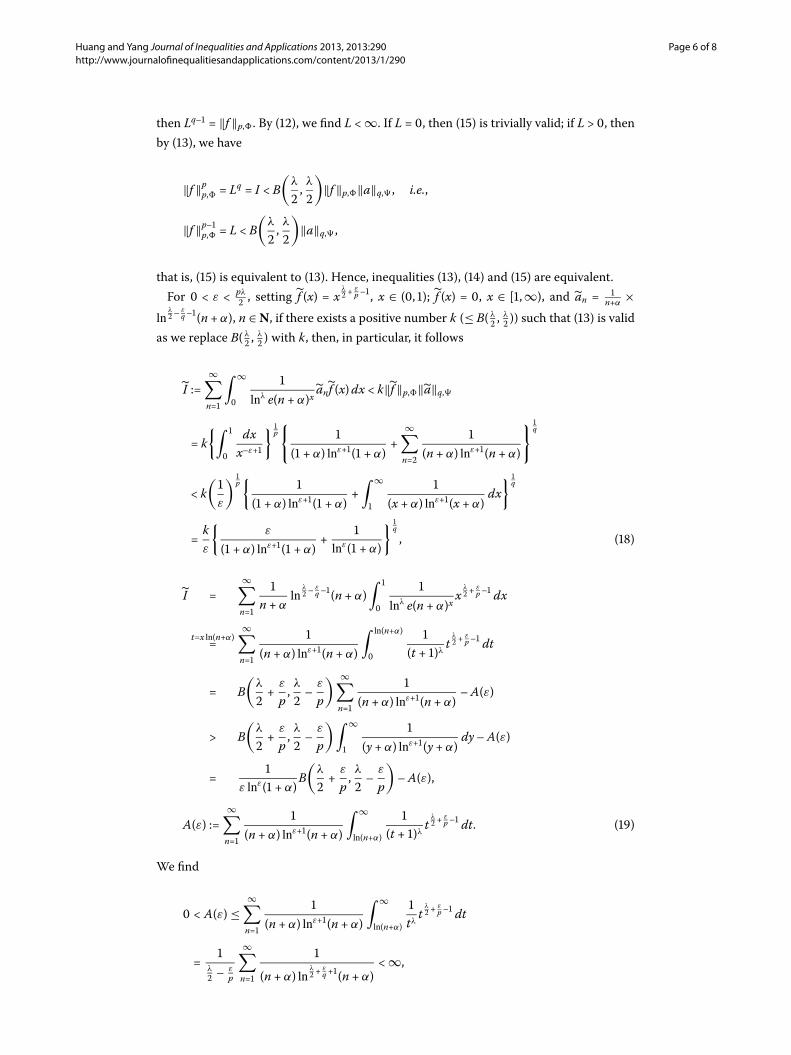
then Lq– = ‖f ‖p,. By (), we find L <∞. If L = , then () is trivially valid; if L > , thenby (), we have
‖f ‖pp, = Lq = I < B(
λ
,λ
)‖f ‖p,‖a‖q, , i.e.,
‖f ‖p–p, = L < B(
λ
,λ
)‖a‖q, ,
that is, () is equivalent to (). Hence, inequalities (), () and () are equivalent.For < ε < pλ
, setting f (x) = xλ +
εp–, x ∈ (, ); f (x) = , x ∈ [,∞), and an =
n+α×
lnλ –
εq–(n + α), n ∈N, if there exists a positive number k (≤ B( λ
,λ )) such that () is valid
as we replace B( λ ,
λ ) with k, then, in particular, it follows
I :=∞∑n=
∫ ∞
lnλ e(n + α)x
anf (x)dx < k‖f ‖p,‖a‖q,
= k{∫
dxx–ε+
} p{
( + α) lnε+( + α)
+∞∑n=
(n + α) lnε+(n + α)
} q
< k(ε
) p{
( + α) lnε+( + α)
+∫ ∞
(x + α) lnε+(x + α)
dx}
q
=kε
{ε
( + α) lnε+( + α)+
lnε( + α)
} q, ()
I =∞∑n=
n + α
lnλ –
εq–(n + α)
∫
lnλ e(n + α)x
xλ +
εp– dx
t=x ln(n+α)=∞∑n=
(n + α) lnε+(n + α)
∫ ln(n+α)
(t + )λ
tλ +
εp– dt
= B(
λ
+
ε
p,λ
–
ε
p
) ∞∑n=
(n + α) lnε+(n + α)
–A(ε)
> B(
λ
+
ε
p,λ
–
ε
p
)∫ ∞
(y + α) lnε+(y + α)
dy –A(ε)
=
ε lnε( + α)B(
λ
+
ε
p,λ
–
ε
p
)–A(ε),
A(ε) :=∞∑n=
(n + α) lnε+(n + α)
∫ ∞
ln(n+α)
(t + )λ
tλ +
εp– dt. ()
We find
< A(ε)≤∞∑n=
(n + α) lnε+(n + α)
∫ ∞
ln(n+α)
tλt
λ +
εp– dt
=
λ –
εp
∞∑n=
(n + α) lnλ +
εq +(n + α)
<∞,
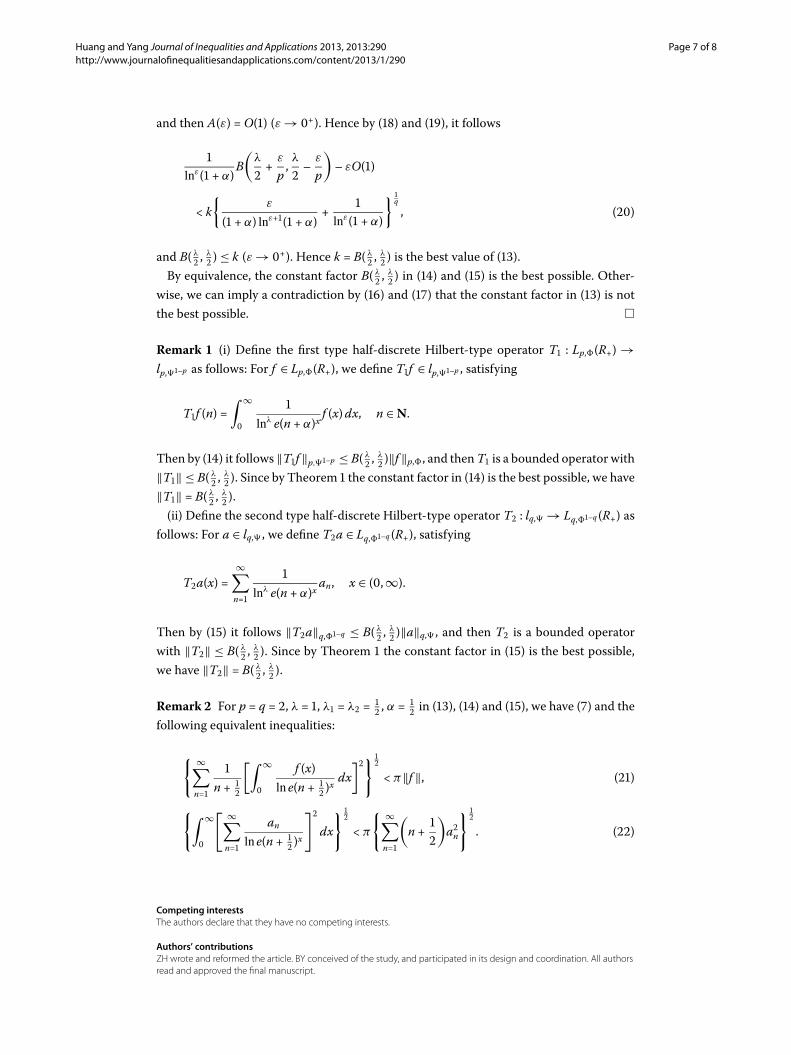
Huang and Yang Journal of Inequalities and Applications 2013, 2013:290 Page 7 of 8http://www.journalofinequalitiesandapplications.com/content/2013/1/290
and then A(ε) =O() (ε → +). Hence by () and (), it follows
lnε( + α)
B(
λ
+
ε
p,λ
–
ε
p
)– εO()
< k{
ε
( + α) lnε+( + α)+
lnε( + α)
} q, ()
and B( λ ,
λ )≤ k (ε → +). Hence k = B( λ
,λ ) is the best value of ().
By equivalence, the constant factor B( λ ,
λ ) in () and () is the best possible. Other-
wise, we can imply a contradiction by () and () that the constant factor in () is notthe best possible. �
Remark (i) Define the first type half-discrete Hilbert-type operator T : Lp,(R+) →lp,–p as follows: For f ∈ Lp,(R+), we define Tf ∈ lp,–p , satisfying
Tf (n) =∫ ∞
lnλ e(n + α)x
f (x)dx, n ∈N.
Then by () it follows ‖Tf ‖p.–p ≤ B( λ ,
λ )‖f ‖p,, and thenT is a bounded operator with
‖T‖ ≤ B( λ ,
λ ). Since by Theorem the constant factor in () is the best possible, we have
‖T‖ = B( λ ,
λ ).
(ii) Define the second type half-discrete Hilbert-type operator T : lq, → Lq,–q (R+) asfollows: For a ∈ lq, , we define Ta ∈ Lq,–q (R+), satisfying
Ta(x) =∞∑n=
lnλ e(n + α)x
an, x ∈ (,∞).
Then by () it follows ‖Ta‖q,–q ≤ B( λ ,
λ )‖a‖q, , and then T is a bounded operator
with ‖T‖ ≤ B( λ ,
λ ). Since by Theorem the constant factor in () is the best possible,
we have ‖T‖ = B( λ ,
λ ).
Remark For p = q = , λ = , λ = λ = , α =
in (), () and (), we have () and thefollowing equivalent inequalities:
{ ∞∑n=
n +
[∫ ∞
f (x)ln e(n +
)xdx
]}
< π‖f ‖, ()
{∫ ∞
[ ∞∑n=
anln e(n +
)x
]
dx}
< π
{ ∞∑n=
(n +
)an
}
. ()
Competing interestsThe authors declare that they have no competing interests.
Authors’ contributionsZH wrote and reformed the article. BY conceived of the study, and participated in its design and coordination. All authorsread and approved the final manuscript.
Huang and Yang Journal of Inequalities and Applications 2013, 2013:290 Page 8 of 8http://www.journalofinequalitiesandapplications.com/content/2013/1/290
Author details1Basic Education College of Zhanjiang Normal University, Zhanjiang, Guangdong 524037, P.R. China. 2Department ofMathematics, Guangdong University of Education, Guangzhou, Guangdong 510303, P.R. China.
AcknowledgementsThis work is supported by 2012 Knowledge Construction Special Foundation Item of Guangdong Institution of HigherLearning College and University (No. 2012KJCX0079).
Received: 23 January 2013 Accepted: 30 April 2013 Published: 7 June 2013
References1. Hardy, GH, Littlewood, JE, Pólya, G: Inequalities. Cambridge University Press, Cambridge (1934)2. Mitrinovic, DS, Pecaric, JE, Fink, AM: Inequalities Involving Functions and Their Integrals and Derivatives. Kluwer
Acaremic, Boston (1991)3. Yang, B: Hilbert-Type Integral Inequalities. Bentham Science Publishers, Sharjah (2009)4. Yang, B: Discrete Hilbert-Type Inequalities. Bentham Science Publishers, Sharjah (2011)5. Yang, B: On a new extension of Hilbert’s inequality with some parameters. Acta Math. Hung. 108(4), 337-350 (2005)6. Yang, B: On Hilbert’s integral inequality. J. Math. Anal. Appl. 220, 778-785 (1998)7. Yang, B: The Norm of Operator and Hilbert-Type Inequalities. Science Press, Beijin (2009).8. Yang, B, Brnetic, I, Krnic, M, Pecaric, J: Generalization of Hilbert and Hardy-Hilbert integral inequalities. Math. Inequal.
Appl. 8(2), 259-272 (2005)9. Krnic, M, Pecaric, J: Hilbert’s inequalities and their reverses. Publ. Math. (Debr.) 67(3-4), 315-331 (2005)10. Jin, J, Debnath, L: On a Hilbert-type linear series operator and its applications. J. Math. Anal. Appl. 371, 691-704 (2010)11. Azar, L: On some extensions of Hardy-Hilbert’s inequality and applications. J. Inequal. Appl. 2009, Article ID 546829
(2009)12. Yang, B, Rassias, TM: On the way of weight coefficient and research for Hilbert-type inequalities. Math. Inequal. Appl.
6(4), 625-658 (2003)13. Arpad, B, Choonghong, O: Best constant for certain multilinear integral operator. J. Inequal. Appl. 2006, Article ID
28582 (2006)14. Kuang, J, Debnath, L: On Hilbert’s type inequalities on the weighted Orlicz spaces. Pac. J. Appl. Math. 1(1), 95-103
(2007)15. Zhong, W: The Hilbert-type integral inequality with a homogeneous kernel of –λ-degree. J. Inequal. Appl. 2008,
Article ID 917392 (2008)16. Li, Y, He, B: On inequalities of Hilbert’s type. Bull. Aust. Math. Soc. 76(1), 1-13 (2007)17. Yang, B: A mixed Hilbert-type inequality with a best constant factor. Int. J. Pure Appl. Math. 20(3), 319-328 (2005)18. Yang, B: A half-discrete Hilbert’s inequality. J. Guangdong Univ. Educ. 31(3), 1-7 (2011)19. Yang, B, Chen, Q: A half-discrete Hilbert-type inequality with a homogeneous kernel and an extension. J. Inequal.
Appl. 2011, 124 (2011). doi:10.1186/1029-242X-2011-12420. Kuang, J: Applied Inequalities. Shangdong Science Technic Press, Jinan (2004)21. Kuang, J: Introduction to Real Analysis. Hunan Education Press, Chansha (1996)
doi:10.1186/1029-242X-2013-290Cite this article as: Huang and Yang: On a half-discrete Hilbert-type inequality similar to Mulholland’s inequality.Journal of Inequalities and Applications 2013 2013:290.