on a class of modified newton cotes quadrature …the above formulae reduce to simpson’s rule in...

Journal of Computational and Applied Mathematics 31 (1990) 331-349 North-Holland

On a class of modified Newton quadrature formulae based upon mixed-type interpolation

331

Cotes

G. VANDEN BERGHE, H. DE MEYER * and J. VANTHOURNOUT Laboratoriurn voor Numerieke Wiskunde en Informatica, Rijksuniversiteit Gent, Krijgslaan 281 -S9, B9000 Gent, Belgium

Received 1 June 1989 Revised 6 February 1990

Abstract: We present quadrature rules which integrate exactly not only polynomials up to a certain degree, but also the functions sin kx and cos kx (where k is a free parameter). The formulae we obtain are modified Newton-Cotes formulae. They are derived by replacing the integrand by an interpolation function of the form a cos kx + b sin kx + E.,“;$,xJ based on equally spaced nodes. The total truncation error of the modified quadrature formulae is discussed and a rigorous proof of the error term is given for the modified Simpson’s 4 rule. Numerical examples show the efficiency of the modified rules and the importance of the error term.

Keywords: Numerical quadrature, Newton-Cotes rules, total truncation error, mixed interpolation.

1. Introduction

Recently Ehrenmark [5] introduced a new quadrature formula with step-dependent coefficients, which exactly integrates the functions 1, sin kx and cos kx over an interval [0, 2h]. Herein k denotes a free parameter, which can be eventually interpreted as the angular frequency of an integrand with oscillatory behaviour; the symbol h represents the considered step. Ehrenmark’s method which is an adaptation of the classical three-point Newton-Cotes quadrature formula of the closed type, also called Simpson’s rule, is given by

/, ) ‘“f(x dx = h (f(0) +f(2h)) E

. $:;ts;) +f(h) 2(~;_-c~;;)‘)], (1.1)

withe=kh. The total truncation error (i.e., the difference of the integral value and the quadrature formula)

reads

F(8) = -$ [k2f”(ll)+f(iv)(~)][~ cot fe-3cot2+e-I], if &a, 0 4

where 8 = kh and 17 E [0, 2h].

* This author acknowledges financial support from the National Fund for Scientific Research (N.F.W.O., Belgium).

0377-0427/90/$03.50 0 1990 - Elsevier Science Publishers B.V. (North-Holland)

332 G. Vanden Berghe et al. / Newton-Cotes quadrature formulae

The above formulae reduce to Simpson’s rule in the limit k + 0. In Section 2 we study the possibility of applying Ehrenmark’s method to derive other extended versions of (n + 1)-points Newton-Cotes formulae (n > 1) of closed and open types. In particular, the derivation of analytic expressions for the respective total truncation errors is of much importance.

The classical Newton-Cotes formulae can be derived by replacing under the integral sign the integrand by a suitable interpolation polynomial and error term, constructed with respect to equally spaced nodes and by integrating afterwards. A natural extension consists in using instead of an interpolation polynomial a more general interpolation function of the form

f,(x) = a sin kx + b cos kx + Q,_,(x), (1.3)

with Q,(x) a polynomial of degree m. Herein k denotes again a free parameter as was the case in Ehrenmark’s derivation. This way of working must result in an alternative method for deriving modified Newton-Cotes formulae with step-dependent coefficients. The study of interpolation functions of the type (1.3) and the corresponding error terms has been the subject of two separate papers [2,3]. The main results discussed there, are summarized hereafter. The function fn(x), obeying the conditions f,(jh)=f(jh) (j=O, l,..., n) can be expressed in terms of forward differences, i.e.,

Ap - k2&(x)A”--l - k2&,+1(x + h)An f(O), 1 where s = x/h and &(x) is defined by the recursion relation

with

Go = 5 tan 30 sin kx,

l- cos( kx - +0)

cos $3 .

(1.4

(l-6)

(1*7)

It is worthwhile to remark that the sum in (1.4) describes the classical interpolation polynomial in its Newton forward-difference form. The occurrence of a sine and cosine term in (1.3) gives rise to +-dependent, i.e., k- and h-dependent, terms in (1.4). In [3] it has been proven that the error term associated with (1.4) can be written as

E,(f, X) = h”-‘~~(x)[k’f’“-‘)(~) +f’““‘([)], 0 < 5 < x,, if nkh < 7, (1-8)

whereby the condition upon nkh is only a sufficient condition. In Section 3 the introduction of (1.3) and (1.8) under the integral sign will be studied and in

Section 4 an analytic closed-form expression for the error in four-point numerical quadrature is rigorously derived. Finally, in Section 5 some numerical experiments with the new derived formulae will be discussed.

G. Vanden Berghe et al. / Newton-Cotes quadrature formulae 333

2. Ehrenmark’s technique

Let us firstly apply Ehrenmark’s method, as an illustration, for the derivation of the simplest modified two-points Newton-Cotes formula of the closed type; i.e., a quadrature formula is sought over [0, h] which is exact for the functions sin kx and cos kx. The results obtained by the method of undetermined coefficients is

with

x@) = “k-;;) , 8 = kh. (2.2)

For k 4 0 the formula reduces to the trapezoidal rule. The error term associated to (2.1) is by definition

JV’) = L’f(x) d x - x(@(f(O) +f(h)). (2.3)

Multiplying by k and choosing the symmetrized integration interval [ - ih, :h] instead of [0, h],

(2.3) reads

kP(@ = kj-:::f(x) d x-A(@[+;h) +f(ih)l,

with

1 - cos e A(B)= sinB =tan@.

Differentiating (2.4) with respect to h leads to

k2F’(8)= -+A(B)[S’(+h)-f’(-+h)] -k@‘(B)

(2-4)

(2.5)

:)[f(:h) +f(-:h)]. (2.6) By differentiating (2.5) one obtains a relation between the coefficients occurring in (2.6), i.e.,

cos +e(k(e) - +) = + sin +eA(e). (2.7)

Introducing (2.7) into (2.6) results in

2 cog +e -k2J”(e) A(e) =cos+e[f’(+h)-f’(-+h)]+ksin@[f(th)+f(-:h)].

(2.8) We define the function G(8) by

: G(B) = -kF’(B) 2;;l;ie

= +[f’(+h)-f’(-$h)] +sin @[f(:h)+f(-:h)]. (2.9)


Clearly G( 0) = 0 for h = 0; differentiating G( 13) gives

G’(9) = =$[f”(jh) +f”(-+h) +k2(f(:h) +++h))]

= gIg(ih) +g(-+h)],

where g(x) is defined by

g(x) =f”(x) + k2f(x).

Provided that g(x) is continuous on [ -

such that

g(:h) + g( - :h) = 2&‘).

By this, (2.10) reduces to

: G'(0) = yg(t(h))

or

ih, ih] it follows that a number 6 E [ -

(2.10)

(2.11)

ih, ih] exists

(2.12)

The mean value theorem can be applied as long as cos 47 has a fixed sign in [0, 01, resulting in

G(8)=2k-2g(g(8)) sin@, -:h<$(O)<:h, if 8<T. (2.13)

From (2.9), taking into account (2.13) and (2.5), one obtains:

e Nd -kF(e) = J, 2 COS iq G(q) dv = ~ekp2g(&)) tan2417 dv (2.14)

As long as 8 < 7, the mean-value theorem can again be applied to obtain

-kF(8)=2k-2g(+3))(tan$e-+e), -+h-0(e)+h,

so that the error term reads, taking into account (2.11),

(2.15)

F(B)=2k-3[f”(e)+k2f(e)](+0-tan$9), -+hc~-c+h, if 8<T. (2.16)

This technique, quite useful for modified closed Newton-Cotes formulae with two ((2.1), (2.16)) and three ((l.l), (1.2)) points, does not lead anymore to closed expressions for the error terms of n-points formulas of the closed type with n > 3. For all open-type formulae it is of no practical use for the derivation of error terms. This technique fails in all these cases because one can no longer express the A’( 8)-dependence in the expression for F’(B) in terms of an A( 8)-dependence. This means that relations of the type (2.7) cannot be constructed if more than three points are involved. Therefore other and more powerful derivation techniques are discussed in the following sections.

G. Vanden Berghe et al. / Newton-Cotes quadrature formulae 33.5

3. Quadrature via mixed interpolation

We want to establish a family of closed integration formulae which extends the corresponding family of Newton-Cotes formulae. By means of a translation we can always make the lower limit of the segment of integration coincide with zero, so that we are only concerned with the approximation of integrals of the type /if(x) d x ( c > 0). The main idea consists in replacing the integrand f(x) by an associated interpolation function f,(x) of the type (1.3), i.e.,

@x) dx = J6’h(x) dx + &,(f. x) dx, (3.1)

the last integral representing the total truncation error. Let us furthermore divide the interval [0, c] into m subintervals of equal width h = c/m and label the intersection points in increasing order: x0 = 0, x1 = h, . . . , xj = jh, . . . , x, = mh = c.

The choice of n in (3.1) is still open but it is most natural to consider the case where n = m.

Then, on account of (1.4) we immediately find that

km”f,(x)dx= 5 Ap~(0)jb"n(~)dx-k2A~-1~(O)lbnn~~(x) dx p=o

- ~2~mf(0)~mh&n+,(x + h) dx, (3.2)

with s = x/h. This quadrature formula is clearly composed of two distinct parts: the first part which coincides exactly with the corresponding Newton-Cotes integration formula, and the second part which contains two correction terms involving the functions Gm(x), &,+t(x) and the forward differences A”-’ and A”. Let us analyse in some more detail these correction terms. We recall that in a previous paper [2] the following properties have been demonstrated:

+,,(x + h) = 4,,,(x) + @n-,(x), n 2 1, (3.3) and

r&&h-x)=(-l)“+‘c#&nh+x), n>,O, (3.4)

which shows that for odd (even) values of n, the function G,,(x) is even (odd) with respect to the midpoint inh of the interval [0, nh]. Hence, it is immediately clear that

J

mh G,(X) dx=O if m=even. (3.9

0

Also,

jomh+m+l(x + h) dx = lh(mfl)h&,+l(~) dx = - /OmhA,+l(x) dx, m = odd.

But from (3.3) it follows that

and the combination of both results leads to

Lmh+m+l(x + h) dx = f~mh%nb) dx if m=odd. (3.6)


The integration formula can therefore be rewritten in the following form:

J ,?L (x) dx

= mh 5 Cjm)f(jh) - k2[A”-‘f(O) + :A”f(0)] lmh&(x) dx if m = odd,

(3.7) J=o

~2&f(o)jo”“a,,b) dx if m=even.

Herein the 6”’ are the Newton-Cotes coefficients with the well-known property Xy=oCJ(m) = 1. It is worthwhile to remark that the evaluation of the correction term to Newton-Cotes’ formula now only involves one integration. Whether m be even or odd, in general the remaining integral cannot be simplified and for every given value of m an explicit evaluation in function of k and h will be required.

As an example, let us consider the case m = 2 which will give rise to a modified Simpson’s rule. Since m is even, the integrand of the remaining integral is the function +,(x). The application of (1.5) for n = 3 leads, with the help of (1.7), to

Hence

;(;)‘-;(;)+l- 4siln’is(l- cos@&‘“‘)]. (3-g)

J o2*q,3(x) dx= $ sine-e 1 f3(1- cos e> ’ and the integration formula becomes

i”f(x) dx-i2*f2(x) dx= +h[f(O) ++f(h) +f@h)]

1 sin 8 - 8 3 + 0(1-cos 0) 1 A’f (0).

(3.9)

(3.10)

Substituting herein the forward difference A2f(0) by its expansion f (0) - 2f (h) + f (2h) we retrieve Ehrenmark’s formula (1.1). For calculational purposes, however, the form (3.10) is much more appropriate, as will be verified in Section 5.

Also, for further use, we mention the next two integration formulas of the family, namely:

i3’f (x) dx = /D’“f,(x) dx

= @[f(O) + 3f(h) + 3fW +f(3h)l 3 1 2 sin 30

4 - 2(i-c0se) 3- e cos +e [ A2f (0) + :A’f (O)] , (3.11)

called extended Simpson’s i rule, and

/4hf (4 dx= /04hfq( x > dx = &h [7f (0) + 32f (h) + 12f (2h) + 32f (3h) + 7f (4h)] 0

l-4 cam 8 sin 8 cos 8

3(1- cos e>' - e(i - cos e)' I b4f WI )

(3.12)


called extended Boole’s rule. Besides the derivation of m-points modified Newton-Cotes formulae we are particularly interested in finding closed expressions for the associated error terms. From (3.1) and (1.8) it is clear that the truncation error corresponding to the closed integration formula (3.7) is given by

h”-1 J omh&,(x)[k2f(mp1)(~) +f’m+l)(t)] dx, 0 < 6 < mh, if mhk <T, (3.13)

whereby 5 is a function of x. The integral (3.13) cannot be evaluated directly by simple application of the integral mean-value theorem since G,(x) has zeros at the nodes xi (j = 0, l,..., m) and therefore does not have constant sign over the interval of integration. However, it has been shown in [2] that

&h(x) = (,“+ l)h2Y (3.14)

and in this limit of k = 0, it has been proved by Steffensen [7] that for odd values of m the calculation of the error term can be carried out as if the mean-value theorem were applicable. Since +,(x) is a continuous function of k in the neighbourhood of k = 0, there is some evidence that Steffensen’s method could equally well be applied to our case. Consequently, we conjecture that for odd values of m (3.13) may be replaced by

hm-i[ k2f’“-“(.n) +f(m+i) (n)] L”‘“a(x) dx, O<q<mh, if mkh<T, m=odd.

(3.15)

Notice that on account of the property (3.4) the naive application of the mean-value theorem would leave us for even values of m with a vanishing integral. Nevertheless, and again by analogy with the pure Newton-Cotes situation, that is in the limit as k -+ 0, the following expression for the truncation error can be proposed in the case of even m:

h” [ k2f’“‘( 7) +f(m+2) (v)]~mhcbrn+b) dx, O<q<mh, if mkh<a, m=even.

(3.16)

Indeed, let us consider the application of (3.1) with n = m + 1 (x,+ 1 = c + h). In particular:

~mh.fm+k4 dx = milAp.fco,Jb”“( ;) dx - k2W(0)jomn&n+d~) dx p=o

- k2A~+1f(0)f’+~+2(x + h) dx.

It is well known from the Newton-Cotes case that

lm”( rnt 1) dx=O if m=even.

Also,

(3.18)

imh&,,+2(x + h) dx = fm+ljhGm+,(X) dx = 0 if m = even, (3.19)

(3.17)


because for even values of m the function Grn+* (x) is odd with respect to the point (1 + $m)h. Hence, for the case of m even, the integration formula (3.17) coincides completely with the integration formula (3.7). Thus, with the assumption that the Steffensen trick is applicable even for k # 0, we are led to conjecture that the truncation error may be written in the form (3.16).

It should be noticed that the integral appearing in the error term is always the same as in the corresponding integration formula. In Table 4 (see the Appendix) we list a number of integrals for the values m = 1,. . . , 4. Furthermore, it is apparent from the formulae (3.15) (m = odd) and (3.16) (m = even) that the modified Newton-Cotes integration formula (3.7) produces an exact result when f(x) is a linear combination of sin kx, cos kx and a polynomial of degree not exceeding m - 2 if m is odd, and of degree not exceeding m - 1 if m is even. Hence, it is always preferable to use a quadrature formula with even m, a property which is well known in the pure Newton-Cotes situation and therefore remains valid in its present extended form. Notice also that for m = 1 and m = 2 the conjectured form of the error term leads to results which coincide with (2.16) and (1.2) respectively.

For reasons of completeness a short survey of modified open Newton-Cotes integration formulae is presented in the Appendix. Let us also remark that some properties of the classical Newton-Cotes formulae still remain valid for the modified ones. If one rewrites the right-hand side of (3.7) by substituting the occurring differences in terms of function evaluations in the appropriate nodes one can observe that the sum of all occurring coefficients of the f( jh)‘s still reduces to one and that these coefficients are symmetric with respect to the central intersection point. In Section 5 we shall exploit the precise form (3.15) or (3.16) of the total truncation error and the fact that k is still a free parameter, in order to increase considerably the accuracy of quadrature formulae. In particular, we shall consider the extended quadrature formulae corresponding to the values m = 1, 2, 4.

4. Truncation error for modified rules

Here we want to expose a technique which allows us to prove rigorously that the truncation error for the modified closed Newton-Cotes formulas (3.7) can be written in the form (3.15) or (3.16) for odd and even m respectively. Since a complete analysis for all m falls outside the scope of the present paper, we shall illustrate the technique by considering the case m = 3. The proof makes use of certain properties of extended complete Tchebycheff systems (ECT) which are studied in [6].

For every m >, 2 the ordered set of functions U, := { U,,(X), ui( x), . . . , u,(x)} = {cos kx, sin kx, 1, x,. . . , xmm2 }, forms an ECT-system on any real interval of length less than kn. If such a system is used as a basis for interpolation with interpolation nodes t, G t, < . . . < t,,,

satisfying k( t, - to) < 7, it can be shown that the error term associated with the interpolation of a function f(x) E Ccm+ ‘) can be written in closed form as

&(f; to, ti,..., t,; x) =$Jto, fl,..., t,; x)[to, fl,..., t,, &“,,,f. (4.1)

Herein $,, which is independent of the function f, is defined by

0, (to,...,tm, x) &&O, t, ,...> t,; 4 = ;’ tto t ) > P-2)

U”, ) -.-1 m


where DUm( t,, . . . , t,) denotes the determinant of the matrix [ uj( ti)]y,,=o with the convention that if, for example, ti = t,_* the (i + l)th row [u,(ti)]yeo is replaced by the row [Duj(ti)]yz, (D being the differential operator). The second factor on the right-hand side of (4.1) is the (m + 1)th order divided difference with respect to U, + 1 which is defined as

1 to, t1,...,tm, x](i,+,f= hr,+,(t0Y..J,? xlf) Ql,+,(to,..., t,, 4 ’ (4.3)

where Q,+,(tO,. . . , t,, x ] f) is obtained by replacing in DUm+,(tO,. . . , t,, x) the function u, + 1( x) by f(x). Divided differences satisfy following recursion:

[ to, tl,...J,+l]Umf= [b..., fmlcl,-,f- [tOYJm-ll(/,_,f

[t l,“‘, L]u,-,Um- [tOY-.Jm-l]um_,%n’ Finally, it is shown in [6] that for all x E [to, t,]

(4-4

[tOY.., t,, x](I,+,f= -++I + I-j”-’ f(E) (m - l)! ’

to < a-4 < t,, if k(t, - to) < 71. (4.5)

As a next step it can be shown that the particular function $,,,(O, h, . . . , mh; x) is closely related to the function C&(X) defined in (1.5)-(1.7), i.e.,

+,(O, A,..., mh; x) = k2h”-‘(m - l)!+,(x), m > 1. (4.6) By the substitution of (4.6) and (4.5) into (4.1) we find

E,(f; 0, h,...,mh; x)=h”-1&,,(x)[D”+1+k2D”-‘]f([),

O<(<mh, if mkh<a, (4.7)

which coincides with the expression (1.8) for E,( f, x). In fact, the foregoing analysis provides an alternative proof of the general form of the error term at the level of interpolation.

For further use we finally define symmetrized $-functions corresponding to h = 1 as follows:

$“,(x)=$,(-+m, -+m+l,..., +m-l,+m; x), m21. (4.8) They satisfy the properties

: I/&+~(x) = (m + l)! “,‘,-~ - ( 1

mqCs$+ll) YxlbL m> 1, 2

(4.9)

and

$S,+,(x + +) - C+,(x - +) = m+;(x), m 2 1, (4.10)

which clearly are a reformulation of the properties (1.5) and (3.3), respectively. In the present notation, our final goal consists in proving (keeping h = 1 for simplicity) that

3’2 #;(x)[ -:, - :, :> :, x]u,f dx

=[(D4+k2D2)f(E)]~3$3(x)~ dx, -: <.$-c 5, if 3k-cv. h=l

(4.11)


The second equality follows immediately from (4.8) and (4.6). The proof of the first equality starts with the observation that on account of (4.5)

J 3’2 $s,<x>[ -:, - :, +, 1, &fdx

- 3/2

= J

1’2 $“,(x>[ -:, - +, t, t, &fdx - 3/2

+([-$3 - :, :, 1, t],f)L-;b) dx

i $D4 + D”):f(ql)]J;::2ji;b) dx, = /1’2 $;(x>[-:, - :, :, :, &,fdx+ [

- 3/2

-- :-e-G, -; <ql < +,

since

(4.12)

does not change sign in [i, $1 when k -C i7r. Furthermore, by means of (4.4) we obtain

I= J ;;;2G(x)[ - :> - :, :, :, x] c/J dx

[-:, -t, :, &f- [-5, - +, t, ;]cJJ =

(u4b) =x2)

=J_;;;+;(x+i)(i-i, -:,:,&J-[A -t,:,:1

where in the last step we used the property that

with

#“,(x)=x- %$.

Since #; is an odd function of x, the integral I can be further simplified, i.e.,

I= /

Il$;(x)[-f. - :, :, x- i]u,fdx

= - j-++([ -:, - i, t, x - &,f) dx>

with

Q(x) = j-);(r) dt,

(4.13)

uJ) dx, (4.14)

(4.15)

(4.16)

(4.17)

(4.18)


and consequently Q( - 1) = Q(1) = 0. It can be verified by fully expanding the relevant determi- nants that

D( [-5, -iA, x-&J)=([-3, 4,:

Hence,

> x-f, x- t]uJ)D

(4.19)

[-4, -+,4,x-+,x-&fdx. (4.20)

If Q(x)W”,(x - :>/U41 h as constant sign on [ - 1, l] we can apply the mean-value theorem and we obtain:

I= $D~+ ~~ :f(n2) i ) [

-/_ile(x)D (‘$(--,i,j dx

= SD4 + D2)ff(~2)j-3(x - :> dx

= -$D4 + D’)if(~j~)j-;;;~$;(x) dx, -: (772 < :. (4.21)

Since the two integrals

J r?;(x) dx = : - : cot*:k + k cot k and

/ 1::,+;(x) dx = - 5 - cot2+k + ; cot :k

yield negative values when 0 < k < ~TI we obtain by combining (4.12) and (4.20) the first equality in (4.11). We still have to prove that Q(x)D[( $;( x - :))/$S,( x)] does not change sign on [ - 1, 11. It is easily verified that for k < T, Q(x) is a nonnegative function on [ - 1, 11. Further- more,

G(x - i) sin :kx - x sin $k

G b> = -1+2cos :k(sin :kx+x sin ik) sin kx_x sink . (4.22)

Now (sin +kx + x sin ik) is an odd function of x which increase on [ - 1, l] if k < T and it can also be shown that (sin :kx - x sin :k)/(sin kx - x sin k) is an even function of x which increases on [0, l] if k < T. It follows that for k < T, D[ @(x - +)/J/S,< x)] is a nonnegative function on [ - 1, l] and therefore the same holds for Q( x)D[ #;( x - i)/$“,( x)], which completes the proof. It should be remarked that the given proof is quite analogous to the proof which has been formulated by Steffensen for the purely polynomial case [7]. It is therefore reasonable to expect that also for every m > 3 a similar extension of Steffensen’s approach could be formulated. We hope to report on this generalization in the near future.


5. Numerical applications

It is our aim to investigate on a few examples whether the newly proposed quadrature formula (3.7) for any particular value of m, performs better than the corresponding Newton-Cotes formula.

Firstly, it should be noticed that the modification of Newton-Cotes’ formulae in the sense of (3.7) does not require more function-value evaluations. Indeed, the correction terms induced by the modification involve forward differences which are easily calculated by establishing a difference scheme built from an ordered set of already known function values.

Furthermore, we still have at our disposal a free parameter k which can be conveniently chosen in the following manner. According to (3.15) (m = odd) or (3.16) (m = even) we attribute to k* a numerical value which implies that the function

x -+ k2f(m-1+6)(X) +f(m+1+6)(~) with 6 = 0 ifm=odd, 1 if m=even, (5.1)

vanishes in at least one point of the integration interval. In all the following examples we have chosen this point to be the midpoint of that interval, i.e.,

f (m+l+w(+mq

k2 = - f (m-1+6)(;mq (5 4

A consequence of the choice (5.2) is that negative values of k* are not excluded. In that case, k

becomes a purely imaginary number and in order to keep all function arguments real it is sufficient to replace systematically in all previous formulae the trigonometric functions by their hyperbolic equivalents. Moreover, it turns out that no further restrictions on the value of kh

should be imposed when using such transformed formulae. The evaluation of the numerical value of k via (5.2) is straightforward when the derivatives of

the integrand f(x) of the required orders can be calculated in closed analytic form. Otherwise, a computational scheme must be set up to approximate these derivatives numerically, and preferably the calculations should only involve already established function values. In particular it is advantageous to use quadrature formulae with even m, since then the middle of the interval belongs to the set of interpolation points.

In practice, we shall divide the interval of integration into N subintervals of equal length. On each of the subintervals the same quadrature formula of the type (3.7) will be applied with some fixed value of m. Hence, care must be taken to relocate the lower limit of the interval. The strategy (5.2) implies that the value of k* differs from subinterval to subinterval. The idea itself of letting k* vary over the total interval of integration has been introduced by Ehrenmark [5]. Indeed, in one of the examples considered in that paper different ad hoc prescriptions for the calculation of k* are studied. Our strategy (5.2), however, has the advantage that it is related to considerations concerning the error bound and that it can be applied to a wide class of integrands f(x).

The three examples analyzed hereafter should provide us with answers to the following questions: - What is the gain of accuracy generally obtained by modifying the closed Newton-Cotes

quadrature formulae in the sense of (3.7)? _ How does the accuracy of the results depend upon m and N?


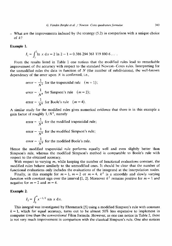
_ What are the improvements induced by the strategy (5.2) in comparison with a unique choice of k?

Example 1.

I1 = s

21nxdx=21n2-1=0.3862943611198906... .

1

From the results listed in Table 1 one notices that the modified rules lead to remarkable improvement of the accuracy with respect to the standard Newton-Cotes rules. Interpreting for the unmodified rules the data in function of N (the number of subdivisions), the well-known dependency of the error upon N is confirmed, i.e.,

error - _T i for the trapezoidal rule (m = 1) ;

error - 7 i for Simpson’s rule (m = 2);

A similar

error - L N6 for Boole’s rule (m = 4).

study for the modified rules gives numerical evidence that there is in this example a gain factor of roughly l/NL, namely

error - s for the modified trapezoidal rule;

error - -$ for the modified Simpson’s rule;

error - -$ for the modified Boole’s rule.

Hence the modified trapezoidal rule performs equally well and even slightly better than Simpson’s rule, whereas the modified Simpson’s method is comparable to Boole’s rule with respect to the obtained accuracy.

With respect to varying m, while keeping the number of functional evaluations constant, the modified rules behave similarly to the unmodified ones. It should be clear that the number of functional evaluations only includes the evaluations of the integrand at the interpolation nodes.

Finally, in this example for m = 1, m = 2 or m = 4, k2 is a smoothly and slowly varying function with constant sign over the interval [l, 21. Moreover k2 remains positive for m = 1 and negative for m = 2 and m = 4.

Example 2.

I2 = /

71,-l/2 sin x dx. 0

This integral was investigated by Ehrenmark [5] using a modified Simpson’s rule with constant k = 1, which for equal accuracy, turns out to be almost 50% less expensive to implement in computer time than the conventional Filon formula. However, as one can notice in Table 2, there is not very much improvement in comparison with the classical Simpson’s rule. One also notices

Tab

le

1

Nu

mer

ical

re

sult

s ob

tain

ed

for

I,

wit

h

the

(mod

ifie

d)

trap

ezoi

dal,

(m

odif

ied)

S

imps

on’s

an

d (m

odif

ied)

B

ook’

s ru

les

Nu

mb

er

of

N

fun

ctio

nal

eval

uat

ion

s

21

20

41

40

61

60

81

80

101

100

121

120

141

140

161

160

181

180

201

200

Mod

ifie

d tr

apez

oida

l T

rape

zoid

al

rule

(m=

l)

rule

(m

=

1)

0.38

6294

2958

5710

0

0.38

6294

3564

8584

3

0.38

6294

3601

3995

7

0.38

6294

3607

9529

9

0.38

6294

3609

8231

3

0.38

6294

3610

5172

0

0.38

6294

3610

8226

1

0.38

6294

3610

9741

0

0.38

6 29

4361

105

623

0.38

6294

3611

1039

3

N

Mod

ifie

d S

imps

on’s

S

imps

on’s

rule

(m=

2)

rule

(m

=

2)

N

Mod

ifie

d B

ook’

s B

OO

k’S

rule

(m=

4)

rule

(m

=

4)

0.38

6190

2096

3220

6 10

0.

386

294

3610

53

336

0.38

6294

3005

9435

7 5

0.38

6 29

4 36

1115

84

0 0.

3862

9436

0380

327

0.38

6268

3204

0247

2 20

0.

3862

9436

1118

843

0.38

6294

3573

2589

4 10

0.

3862

9436

1119

874

0.38

6 29

4 36

1107

99

7

0.38

6282

7872

3334

3 30

0.

3862

9436

1119

799

0.38

6294

3603

7004

9 15

0.

3862

9436

1119

890

0.38

6294

3611

1884

1

0.38

6287

8507

6256

1 40

0.

3862

9436

1119

874

0.38

6294

3608

8259

0 20

0.

3862

9436

1119

891

0.38

6294

3611

1970

4

0.38

6290

1944

7752

9 50

0.

3862

9436

1119

886

0.38

6 29

4 36

1022

68

4 25

0.

3862

9436

1119

891

0.38

6294

3611

1984

2

0.38

6291

4676

1309

3 60

0.

3862

9436

1119

889

0.38

6294

3610

7301

0 30

0.

3862

9436

1119

891

0.38

6294

3611

1987

4

0.38

6 29

2 23

5 27

5 87

7 70

0.

3862

9436

1119

890

0.38

6294

3610

9458

5 35

0.

3862

9436

1119

891

0.38

6294

3611

1988

4

0.38

6292

7335

1943

3 80

0.

3862

9436

1119

891

0.38

6294

3611

0505

7 40

0.

3862

9436

1119

891

0.38

6294

3611

1988

8

0.38

6293

0751

1397

6 90

0.

3862

9436

1119

891

0.38

6294

3611

1063

0 45

0.

3862

9436

1119

891

0.38

6294

3611

1988

9

0.38

6293

3194

5474

3 10

0 0.

3862

9436

1119

891

0.38

6294

3611

1381

5 50

0.

3862

9436

1119

891

0.38

6294

3611

1989

0


Table 2 Numerical results obtained for I2 with the (modified) Simpson’s and (modified) Boole’s rules

Number of Simpson’s rule Boole’s rule functional N Modified Modified N evaluations

Classical Modified Classical (k calculated) (k =l)

201 100 1.789 545 999 1.789503 108 1.789503 112 50 1.789 548 991 1.789522593 401 200 1.789 621598 1.789606431 1.789606431 100 1.789622651 1.789613319 601 300 1.789 640436 1.789632180 1.789632180 150 1.789641009 1.789635 929 801 400 1.789 648 323 1.789642960 1.789642960 200 1.789648695 1.789645 395

1001 500 1.789652480 1.789648643 1.789 648 643 250 1.789652746 1.789650386

that with the choice (5.2) the accuracy really improves. In Fig. 1 we show how 1 k 1 sign( k2)

varies over the integration interval for both cases m = 2 and m = 4. Evidently, in this example keeping the value of k constant over the entire interval [0, IT] is a too severe restriction which on account of (3.16) induces relevant contributions to the error term. On the other hand, it is clear

klsignfk’)

S

b

Fig. 1. Plot of j k 1 sign(k2) against x for the modified Simpson’s rule and the modified Boole’s rule for the integral considered in Example 2. Also, k2 is the real value calculated from (5.2). The modified Simpson’s rule (m = 2) is

denoted by ‘s’, the modified Boole’s rule (m = 4) is denoted by ‘b’. The values of x are restricted to IO, a].


Table 3 Numerical results obtained for Z, with the (modified) Simpson’s and (modified) Boole’s rules

Number of functional evaluations

Simpson’s rule

N Modified Classical

Boole’s rule

N Modified Classical

221 110 0.060704631 0.052963 214 55 0.060 738 568 0.041912 353 441 220 0.059 870 100 0.059 577 889 110 0.059838092 0.060018 867 661 330 0.059839 941 0.059791870 165 0.059 839 931 0.059 850444 881 440 0.059 839 800 0.059 825058 220 0.059 839 863 0.059 841536

from the curves displayed in Fig. 1 that with each extended rule (m = 2 or m = 4) some positive real values of k are attained which violate the condition mhk < T. One should, however, keep in mind that this is only a sufficient condition. Moreover, the present example shows that by accepting values of k which violate this condition the truncation error remains sufficiently small.

Example 3. As a last example we consider the integral

I3 = J

2nx sin 20x cos 50x dx = 0

&T = 0.059 839 860 . . .)

which stands as a model of rapidly oscillatory integrals. This example was also investigated by Duris [4], by Davis and Rabinowitz [l] and by Ehrenmark [5]. Table 3 shows that also for this type of integral our method is very appropriate in spite of the fact that the used values of k2

fluctuate rapidly over the range of integration and also that at certain nodes extremely large values of k* are generated.

6. Conclusion

Our goal was the derivation of quadrature rules which integrate exactly polynomials up to a certain degree and the two functions sin kx and cos kx. Since the technique of Ehrenmark is only appropriate for 2- and 3-point formulas of the closed type, a more powerful technique was needed. We established (m + l)-point formulae which we call modified Newton-Cotes rules. They are obtained by replacing the integrand by a mixed-type interpolation function a cos kx +

b sin kx + Cy=&%jxj, based on equally spaced nodes. The total truncation error can be estimated since the error at interpolation level is known. We learn from the discussion of the error term that, as was the case with the classical Newton-Cotes formulae, it is recommended to use (m + l)-points formulae where m is even. We derived rules of the closed and open type.

The implementation of the formulae does not require more function evaluations than in the classical polynomial case. By exploiting the form of the total truncation error a new strategy for attributing a varying value to the parameter k is proposed and the gain in accuracy with respect to the classical rules shows to be significant. The modified rules are especially appropriate for oscillating integrands.


Appendix

In order to derive extended open Newton-Cotes integration formulae we start from the equality

imhf(x) dx = im’L_2(x) dx + i”“$-,(f, x) dx, (A4 where fi_,( x) is the interpolation function at the n - 1 points x1 = h, x2 = 2h,. . . , x,-~ =

(n - 1)h. It follows from (1.4) after moving the origin that

L-,(x> = ;!I(‘; ‘)ayf(h) - k2[$-,(x - h)An-3f(h) + A-,(xF2f(h)],

s=x h’ 64.2)

Again, it is reasonable to choose n = m, and a similar reasoning as before leads to

4mhA-2(x) dx =

m-1

mh c Dj’“‘f(jh) - I k2 [2Ame3f( h) + AmP2f( h)] ~mh+m_,( x) dx if m = odd,

j=l k2A”-‘f( h)~mn+m_l(x) dx if m = even,

(A-3)

where D!“’ are the coefficients of the open Newton-Cotes formulae which satisfy C’JLtDjm) = 1. As eximples of both m even and odd, we calculate

Julh~,(x) dx= ~[~ + “““,‘“,,~” “1

and 2 sin 29

l-co.58 + 8(1-cos8) * 1 Using these, the respective open integration formulae become

i’“r;cX) dx=ih[f(h)+f(2h)] -h(2f(h)+Af(h)][$ + “““,‘“,,“,“” “1

and

L x dx = :h[2f(h) -f(2h) + 2f(3h)] ( )

2 h[Af(h)] [

8 - 7

-

=h[f(h) +f(3h)

2 I sin 28 1

1 - cos e + e(l - cos e) ]

(A4

(A.9

(A-6)


Finally, it is easy to see that for the truncation error the following expression can be conjectured:

hm-3[ k2f’-3’ (q) +f(mP1)(q)]jb”h$+,,_2(x - h) dx, 0 -Z q < mh, if mkh -c 7,

(A.8)

on condition that the integral is different from zero. This is indeed the case for odd values of m, and then (A.8) can be rewritten in the form

2h”-3[k2f’“-3’(~) +~‘““(s)]lom”a-,(x) dx,

O-cq-cmh, if mkh<T, m=odd. (A-9)

If m is even, a similar reasoning as in Section 3 proves that the error term is expected to be given

by

h-2 [ k2f’“-2’ (4 +f’“‘h)] ,$?dx - h) dx,

O<v<m/i, if mkh<n, m=even, (A.lO)

which can also be rewritten as

h-2 [ k2f’“-2’ (‘1)+f(~)(9)]ldnn~~_~(x) dx, O<q<mh, if mkh<+n, m = even.

(All)

It should be noticed that the integrals occurring in (A.9) and (All) are formally the same. For practical purposes these integrals as well as those encountered in Section 3 are listed in Table 4 for the values m = 1,. . . ,4.

Table 4 Certain integrals arising in the closed quadrature formulas (3.7) and corresponding error terms (3.15), (3.16) and in the open quadrature formulas (A.3) and corresponding error terms (A.9)-(A.11)

m k2 mh+,,,(x) d 7;-” /

x k2 mh~ To / m+l (x)d X k2 mh+ _ (x)d Torn1 x

/

2(1-cos8) 1 l-case 1 1_ 2sin8(1-cosB) O sin fl 2 + (3 sine e(l+cos e)

2 0 1 1 sin e --l-+ 3 efi-c0s e)

2_ 2sine e

3‘ ’ 3 3 i+2c0se 3 1+2cos e 3 3 (I-~~s~)(~+~cos~) - _- -- 4 2(i-c0se)

+ BsinB

-8+ 4(1-~0~8) 28sinO 2 e sin e

4 0 14 l-4c0s e sin e cos e 8 2 2 sin e cos e -- 15 3(1 -cos e)’ - e(i-c0s e)’ 7-1+ e(l-cOse)


References

[l] P.J. Davis and P. Rabinowitz, Methods of Numerical Integration (Academic Press, New York, 1984). [2] H. De Meyer, J. Vanthoumout and G. Vanden Berghe, On a new type of mixed interpolation, J. Comput. Appl.

Math. 30 (1) (1990) 55-69. [3] H. De Meyer, J. Vanthoumout, G. Vanden Berghe and A. Vanderbauwhede, On the error estimation for a mixed

type of interpolation, J. Comput. Appl. Math. (1990), to appear.

[4] C.S. Duris, Generating and compounding product-type Newton-Cotes quadrature formulas, TOMS 2 (1976) 50-58.

[5] U.T. Ehrenmark, A three-point formula for numerical quadrature of oscillatory integrals with variable frequency, J. Comput. Appl. Math. 21 (1) (1988) 87-99.

[6] L.L. Schumaker, Spiine Functions: Basic Theory (Wiley, New York, 1981). [7] J.F. Steffensen, Interpolation (Williams and Wilkins, Baltimore, MD, 1927); (Chelsea, New York, 2nd ed., 1950).

on a class of modified newton cotes quadrature …the above formulae reduce to simpson’s rule in...

Documents