omnibus user manual
TRANSCRIPT

ORNL/TM-2018/1073
Omnibus User Manual
Approved for public release.Distribution is unlimited.
Seth R. JohnsonThomas M. EvansGregory G. DavidsonSteven P. HamiltonTara M. PandyaKatherine E. RoystonElliott D. Biondo
Aug. 2020

DOCUMENT AVAILABILITYReports produced after January 1, 1996, are generally available free via US Department of Energy(DOE) SciTech Connect.
Website osti.gov
Reports produced before January 1, 1996, may be purchased by members of the public from thefollowing source:
National Technical Information Service5285 Port Royal RoadSpringfield, VA 22161Telephone 703-605-6000 (1-800-553-6847)TDD 703-487-4639Fax 703-605-6900E-mail [email protected] classic.ntis.gov
Reports are available to DOE employees, DOE contractors, Energy Technology Data Exchangerepresentatives, and International Nuclear Information System representatives from the followingsource:
Office of Scientific and Technical InformationPO Box 62Oak Ridge, TN 37831Telephone 865-576-8401Fax 865-576-5728E-mail [email protected] osti.gov/contact
This report was prepared as an account of work sponsored by anagency of the United States Government. Neither the United StatesGovernment nor any agency thereof, nor any of their employees,makes any warranty, express or implied, or assumes any legal lia-bility or responsibility for the accuracy, completeness, or usefulnessof any information, apparatus, product, or process disclosed, or rep-resents that its use would not infringe privately owned rights. Refer-ence herein to any specific commercial product, process, or serviceby trade name, trademark, manufacturer, or otherwise, does not nec-essarily constitute or imply its endorsement, recommendation, or fa-voring by the United States Government or any agency thereof. Theviews and opinions of authors expressed herein do not necessarilystate or reflect those of the United States Government or any agencythereof.

ORNL/TM-2018/1073
Reactor and Nuclear Systems Division
OMNIBUS USER MANUAL
Seth R. JohnsonThomas M. Evans
Gregory G. DavidsonSteven P. Hamilton
Tara M. PandyaKatherine E. Royston
Elliott D. Biondo
Date Published: Aug. 2020
Prepared byOAK RIDGE NATIONAL LABORATORY
Oak Ridge, TN 37831-6283managed by
UT-Battelle, LLCfor the
US DEPARTMENT OF ENERGYunder contract DE-AC05-00OR22725


CONTENTS
Contents . . . . . . . . . . . . . . . . . . . . . . . . . . . . . . . . . . . . . . . . . . . . . . . . . . iiiList of Figures . . . . . . . . . . . . . . . . . . . . . . . . . . . . . . . . . . . . . . . . . . . . . . . vList of Tables . . . . . . . . . . . . . . . . . . . . . . . . . . . . . . . . . . . . . . . . . . . . . . . viiAbstract . . . . . . . . . . . . . . . . . . . . . . . . . . . . . . . . . . . . . . . . . . . . . . . . . . 11. Introduction . . . . . . . . . . . . . . . . . . . . . . . . . . . . . . . . . . . . . . . . . . . . . . 1
1.1 Omnibus execution . . . . . . . . . . . . . . . . . . . . . . . . . . . . . . . . . . . . . . . 11.2 Python bindings . . . . . . . . . . . . . . . . . . . . . . . . . . . . . . . . . . . . . . . . . 21.3 Post-processing tools . . . . . . . . . . . . . . . . . . . . . . . . . . . . . . . . . . . . . . 2
2. Front End Interface . . . . . . . . . . . . . . . . . . . . . . . . . . . . . . . . . . . . . . . . . . 52.1 Running Omnibus . . . . . . . . . . . . . . . . . . . . . . . . . . . . . . . . . . . . . . . . 52.2 Omnibus ASCII Input Format . . . . . . . . . . . . . . . . . . . . . . . . . . . . . . . . . 72.3 Omnibus input and output . . . . . . . . . . . . . . . . . . . . . . . . . . . . . . . . . . . . 102.4 Errors, warnings, and other messages . . . . . . . . . . . . . . . . . . . . . . . . . . . . . . 132.5 Command line tools . . . . . . . . . . . . . . . . . . . . . . . . . . . . . . . . . . . . . . . 15
3. Omnibus Input Description . . . . . . . . . . . . . . . . . . . . . . . . . . . . . . . . . . . . . . 253.1 Omnibus input file contents . . . . . . . . . . . . . . . . . . . . . . . . . . . . . . . . . . . 253.2 Problem attributes: [PROBLEM] . . . . . . . . . . . . . . . . . . . . . . . . . . . . . . . . 273.3 Execution: [RUN] . . . . . . . . . . . . . . . . . . . . . . . . . . . . . . . . . . . . . . . . 293.4 Output options: [OUTPUT] . . . . . . . . . . . . . . . . . . . . . . . . . . . . . . . . . . . 393.5 Model definition: [MODEL] . . . . . . . . . . . . . . . . . . . . . . . . . . . . . . . . . . 433.6 MCNP input: [MODEL=mcnp] . . . . . . . . . . . . . . . . . . . . . . . . . . . . . . . . 443.7 SCALE input: [MODEL=scale] . . . . . . . . . . . . . . . . . . . . . . . . . . . . . . . . 503.8 Geometria input: [MODEL=geometria] . . . . . . . . . . . . . . . . . . . . . . . . . . . . 523.9 Reactor ToolKit input: [MODEL=rtk] . . . . . . . . . . . . . . . . . . . . . . . . . . . . . 533.10 Brick mesh input: [MODEL=mesh] . . . . . . . . . . . . . . . . . . . . . . . . . . . . . . 533.11 Geant4 input: [MODEL=geant] . . . . . . . . . . . . . . . . . . . . . . . . . . . . . . . . 543.12 SWORD input: [MODEL=sword] . . . . . . . . . . . . . . . . . . . . . . . . . . . . . . . 543.13 DAGMC input: [MODEL=dagmc] . . . . . . . . . . . . . . . . . . . . . . . . . . . . . . . 553.14 VERA input: [MODEL=vera] . . . . . . . . . . . . . . . . . . . . . . . . . . . . . . . . . 563.15 Particle source definitions: [SOURCE] . . . . . . . . . . . . . . . . . . . . . . . . . . . . . 563.16 Physics engines: [PHYSICS] . . . . . . . . . . . . . . . . . . . . . . . . . . . . . . . . . . 853.17 Continuous-energy physics: [PHYSICS=ce] . . . . . . . . . . . . . . . . . . . . . . . . . . 853.18 Multigroup physics: [PHYSICS=mg] . . . . . . . . . . . . . . . . . . . . . . . . . . . . . 963.19 Compositions: [COMP] . . . . . . . . . . . . . . . . . . . . . . . . . . . . . . . . . . . . . 1063.20 Responses: [RESPONSE] . . . . . . . . . . . . . . . . . . . . . . . . . . . . . . . . . . . 1113.21 Tallies: [TALLY] . . . . . . . . . . . . . . . . . . . . . . . . . . . . . . . . . . . . . . . . 1133.22 Shift Monte Carlo solver: [SHIFT] . . . . . . . . . . . . . . . . . . . . . . . . . . . . . . . 1673.23 Denovo deterministic solver: [DENOVO] . . . . . . . . . . . . . . . . . . . . . . . . . . . 1763.24 ORIGEN depletion solver: [DEPLETION] . . . . . . . . . . . . . . . . . . . . . . . . . . . 2123.25 Hybrid methodology: [HYBRID] . . . . . . . . . . . . . . . . . . . . . . . . . . . . . . . . 2243.26 Pre-execution utilities: [PRE] . . . . . . . . . . . . . . . . . . . . . . . . . . . . . . . . . . 2273.27 Post-processing: [POST] . . . . . . . . . . . . . . . . . . . . . . . . . . . . . . . . . . . . 229
4. Geometria Input Description . . . . . . . . . . . . . . . . . . . . . . . . . . . . . . . . . . . . . 2334.1 Geometria input file contents . . . . . . . . . . . . . . . . . . . . . . . . . . . . . . . . . . 2334.2 Universe definitions: [UNIVERSE] . . . . . . . . . . . . . . . . . . . . . . . . . . . . . . 2344.3 Shape definitions: [UNIVERSE][SHAPE] . . . . . . . . . . . . . . . . . . . . . . . . . . . 246
iii

References . . . . . . . . . . . . . . . . . . . . . . . . . . . . . . . . . . . . . . . . . . . . . . . . . 2675. Acknowledgments . . . . . . . . . . . . . . . . . . . . . . . . . . . . . . . . . . . . . . . . . . . 269A. Examples . . . . . . . . . . . . . . . . . . . . . . . . . . . . . . . . . . . . . . . . . . . . . . . A–2
A.1 Visualization . . . . . . . . . . . . . . . . . . . . . . . . . . . . . . . . . . . . . . . . . . A–3A.2 Denovo . . . . . . . . . . . . . . . . . . . . . . . . . . . . . . . . . . . . . . . . . . . . . A–9A.3 Multigroup data exploration . . . . . . . . . . . . . . . . . . . . . . . . . . . . . . . . . .A–91A.4 Shift . . . . . . . . . . . . . . . . . . . . . . . . . . . . . . . . . . . . . . . . . . . . . . .A–103A.5 CE data . . . . . . . . . . . . . . . . . . . . . . . . . . . . . . . . . . . . . . . . . . . . .A–132A.6 Supplemental . . . . . . . . . . . . . . . . . . . . . . . . . . . . . . . . . . . . . . . . . .A–152
B. File format specifications . . . . . . . . . . . . . . . . . . . . . . . . . . . . . . . . . . . . . . . B–2B.1 Denovo Output Specification . . . . . . . . . . . . . . . . . . . . . . . . . . . . . . . . . . B–3B.2 HDF5 Mesh Model Specification . . . . . . . . . . . . . . . . . . . . . . . . . . . . . . . . B–4B.3 RTK XML Input Specification . . . . . . . . . . . . . . . . . . . . . . . . . . . . . . . . . B–5B.4 XS XML Input Specification . . . . . . . . . . . . . . . . . . . . . . . . . . . . . . . . . . B–5
iv

LIST OF FIGURES
1 Execution flow for omnibus-run. The small black boxes are the typical input/output files,blue circles are parts of the Python pre-processor run on the head node, the red circle is theOmnibus executable (run on the compute nodes), and dotted lines denote optional files (e.g.,multiple input files). . . . . . . . . . . . . . . . . . . . . . . . . . . . . . . . . . . . . . . . 11
v

LIST OF TABLES
1 Special characters in Omnibus input. . . . . . . . . . . . . . . . . . . . . . . . . . . . . . . 82 Omnibus diagnostic output examples. . . . . . . . . . . . . . . . . . . . . . . . . . . . . . 14
3 Available types for the [RUN] database . . . . . . . . . . . . . . . . . . . . . . . . . . . . . 294 Feature matrix for the supported models. . . . . . . . . . . . . . . . . . . . . . . . . . . . . 435 Available types for the [MODEL] database . . . . . . . . . . . . . . . . . . . . . . . . . . . 446 Mappings between unusual nuclide IDs. . . . . . . . . . . . . . . . . . . . . . . . . . . . . 457 Mappings between MCNP MT cards and SCALE IDs. . . . . . . . . . . . . . . . . . . . . 468 Available types for the [MOVABLE] database . . . . . . . . . . . . . . . . . . . . . . . . . 499 MOAB volume properties used in the DAGMC model. . . . . . . . . . . . . . . . . . . . . 5510 Available types for the [SOURCE] database . . . . . . . . . . . . . . . . . . . . . . . . . . 5711 Available types for the [SHAPE] database . . . . . . . . . . . . . . . . . . . . . . . . . . . 6612 Available types for the [ENERGY] database . . . . . . . . . . . . . . . . . . . . . . . . . . 6613 Available types for the [ANGLE] database . . . . . . . . . . . . . . . . . . . . . . . . . . . 6614 Available types for the [SPECTRUM] database . . . . . . . . . . . . . . . . . . . . . . . . 6615 Available types for the [PHYSICS] database . . . . . . . . . . . . . . . . . . . . . . . . . . 8516 SCALE CE library path aliases in SCALE 6.2. . . . . . . . . . . . . . . . . . . . . . . . . . 8617 Default DBRC data paths in SCALE 6.2. . . . . . . . . . . . . . . . . . . . . . . . . . . . . 8818 Available types for the [SPLICE] database . . . . . . . . . . . . . . . . . . . . . . . . . . . 9319 Multigroup physics library aliases and filenames in SCALE 6.2. . . . . . . . . . . . . . . . 9920 Possible cross section input formats. . . . . . . . . . . . . . . . . . . . . . . . . . . . . . . 10421 GIP reaction tables. . . . . . . . . . . . . . . . . . . . . . . . . . . . . . . . . . . . . . . . 10522 Available types for the [RESPONSE] database . . . . . . . . . . . . . . . . . . . . . . . . . 11123 Available types for the [DIAGNOSTIC] database . . . . . . . . . . . . . . . . . . . . . . . 14024 Available types for the [OUTPUT] database . . . . . . . . . . . . . . . . . . . . . . . . . . 16625 Available types for the [DECOMPOSITION] database . . . . . . . . . . . . . . . . . . . . 16926 Available types for the [GENERATIONS] database . . . . . . . . . . . . . . . . . . . . . . 17527 Denovo spatial discretization options. . . . . . . . . . . . . . . . . . . . . . . . . . . . . . 17928 Available types for the [BOUNDARY] database . . . . . . . . . . . . . . . . . . . . . . . . 18329 Denovo quadrature construction options. . . . . . . . . . . . . . . . . . . . . . . . . . . . . 18530 Denovo quadrature availability matrix. . . . . . . . . . . . . . . . . . . . . . . . . . . . . . 18531 Available types for the [SOLVER] database . . . . . . . . . . . . . . . . . . . . . . . . . . 19232 Denovo solver verbosity options. . . . . . . . . . . . . . . . . . . . . . . . . . . . . . . . . 19833 Available types for the [PRECONDITIONER] database . . . . . . . . . . . . . . . . . . . . 20334 Available types for the [PRECONDITIONER] database . . . . . . . . . . . . . . . . . . . . 20435 Available types for the [PRECONDITIONER] database . . . . . . . . . . . . . . . . . . . . 21136 Available types for the [HYBRID] database . . . . . . . . . . . . . . . . . . . . . . . . . . 22437 Weight window input options. . . . . . . . . . . . . . . . . . . . . . . . . . . . . . . . . . 226
38 Available types for the [UNIVERSE] database . . . . . . . . . . . . . . . . . . . . . . . . . 23439 Available types for the [SHAPE] database . . . . . . . . . . . . . . . . . . . . . . . . . . . 246
vii


ABSTRACT
This manual provides instructions for using the Omnibus front end to the Exnihilo code suite, which containsthe Denovo and Shift transport solvers.
1. INTRODUCTION
Exnihilo is a modern radiation transport framework that implements state-of-the-art algorithms, solvers, andsolution methodologies, enabling it to solve a wide variety of nuclear engineering and applications problemswith the scalability to run on desktop machines and leadership-class supercomputers. The Omnibus code[3] is a powerful, flexible interface to the extensive functionality of Exnihilo. This manual documents theExnihilo capabilities exposed by Omnibus and demonstrates their use.
Omnibus provides access to the two core Exnihilo transport solvers, the Denovo deterministic solver(page 176) [4] and the Shift Monte Carlo solver (page 167) [5]. In addition, Omnibus allows the twosolvers to be coupled using modern hybrid methods (page 224) that accelerate Shift transport solutions usingapproximate solutions from Denovo. Omnibus also allows time-dependent Shift depletion calculations usingthe ORIGEN nuclide depletion solver (page 212) [6].
The Exnihilo transport framework is designed to support computational transport using a combinationof input models (page 43) (which define a problem’s geometry and compositions) and multiple physicsimplementations (page 85) (which implement approximations to the Boltzmann transport equation). Manyclasses of particle sources (page 56) and tallies (page 113) can be defined separately from the model’sgeometry, and custom compositions (page 106) can also be entered by the user.
The Omnibus interface enables other codes such as ADVANTG [7] and SWORD [8] to create, execute, andpost-process Denovo problems, but their use is outside the scope of this document. Other radiation transportcodes such as VERAShift [9] and SCALE [2] use the Shift and Denovo codes through a lower-level interfacevia an internal Omnibus-based API. Although these codes are also outside the scope of this manual, thefeatures and some interfaces presented here may inform the use of downstream codes.
1.1 OMNIBUS EXECUTION
At its core, Omnibus is a high-performance, MPI-enabled binary executable, the input of which is a hierarchi-cal problem definition. The Omnibus executable is designed to be launched by a driver, the omnibus Pythonmodule, which generates a validated input for the executable before launching it in parallel.
Pre-execution validation, which can be run using the omnibus-pre (page 16) command, is critically importantfor high-performance computing (HPC) systems in which tens or hundreds of thousands of CPU hours canpotentially be lost if an invalid input causes a single process to fail. It is also a tremendous time saver onother shared computing resources such as institutional clusters, ensuring that the input does not need to bequeued and launched before it is validated. If a problem input is rejected, then the Python pre-processor canalso construct a descriptive, context-sensitive error message such as:
ERROR: From input at ueki-cadis.omn:19:FATAL ERROR: In /physics/ce, the following unknown inputs were found: 'mood' (did you→mean 'mode'?)
or
1

FATAL ERROR: At ueki-cadis.omn:21: Invalid value 'npe' for keyword 'mode' at /physics/ce/→mode:expected particle transport mode (``n``, ``neutron``, ``np``, ``p``, ``photon``, or→``pn``), but string is not a particle mode[mode: Particles to transport]:
npe
Besides validating the user input and providing error messages, the Python input schemas are also used togenerate the Omnibus (page 25) and Geometria (page 233) input specifications in this manual.
1.2 PYTHON BINDINGS
Exnihilo uses the SWIG1 utility to generate Python interfaces to utility classes in Exnihilo. These interfacespower some Omnibus capabilities such as ray tracing, but they may also be used by power users as a high-levelinterface to many core Exnihilo capabilities, including exploring nuclear data and interacting with problemmodels.
The following Python modules are installed with Exnihilo2:
nemesis: Infrastructure components This collection of utilities includes interfaces to MPI and Silo.
robus: Physics data Robus has containers designed to load and store continuous-energy and multigroupcross sections, nuclides, and compositions.
transcore: Transport core components This package includes cross section storage classes, libraries forreading and writing cross sections, etc. See Multigroup data exploration (page A–91) for an exampleof creating and visualizing multigroup cross sections.
geometria: Geometry interfaces This module has interfaces to the different geometry models used by Shift.It enables ray tracing of the geometry and extraction of compositions.
physica: Physics packages The physics package includes additional interfaces to the CE data. See CE data(page A–132) for examples.
1.3 POST-PROCESSING TOOLS
Several tools have been developed to support interacting with, processing, and visualizing Exnihilo inputand output. Most of the data are read from and written to HDF5 files, so the workflows rely heavily on thePython-based h5py module.
1.3.1 OMNIBUS.DATA
The Omnibus data toolset is an h5py-based interface to Exnihilo HDF5 input and output files. It allows slicesof the data to be taken without loading the entire file into memory, and it includes plotting tools based onmatplotlib. For examples on how to use this module, see the Denovo (page A–9) and Shift (page A–103)example sections.
Note: The full documentation of the postprocessing tools is outside the scope of this manual. However, ifyou’re using IPython (e.g., through omnibus-analysis) or Jupyter notebook to postprocess the data, tab
1 http://sourceforge.net/projects/swig2 SWIG Python bindings will only be available when Exnihilo is built with the SWIG option on and when installing shared
libraries.
2

completion on any of the Omnibus analysis objects will list the available methods for that object. Additionally,adding a question mark symbol after a method or object will provide a help overview showing the argumentsthat function expects. Finally, the help built-in function provides detailed information about available datamembers and methods of any object.
1.3.2 [POST] BLOCK
When run through omnibus-run (page 15), the post-processing block in the Omnibus input will extractspecified data from the HDF5 output in a more human-friendly format. For example, this block willgenerate an ReST-formatted text file summarizing the run, plot keff values for Shift eigenvalue problems,and generate csv-formatted tables of depletion results. More advanced post-processing blocks such as[DENOVO][SPECTRUM], which will write flux spectra at the given list of points, allow complex extraction ofuser-specified data.
1.3.3 H5SH
The h5sh tool3 provides a shell-like interface to browsing HDF5 files. It can be independently downloadedand installed through Python’s package manager (pip install h5sh).
It can be cumbersome to use the Omnibus python post-processing tools to quickly examine the contents of anExnihilo output (or input) file. Some developers have gotten into the habit of using h5ls and h5dump forthis, but those tools are impossibly slow for files greater than a few hundred megabytes, and it is inconvenientand slow to use them for multiple consecutive invocations to drill down on a piece of data.
To this end, Exnihilo includes a small but powerful tool that allows the user to browse any HDF5 file as if itwere a directory in a shell terminal. HDF5 groups become directories and datasets act as files. It is designedto be intuitive and straightforward. See Using the h5sh tool (page A–152) for an example of its use or theonline documentation4 for more details.
3 https://pypi.org/project/h5sh/4 https://h5sh.readthedocs.io/
3


2. FRONT END INTERFACE
Your Exnihilo installation contains the omnibus executable (which actually drives Denovo and Shift froman XML input file), as well as additional Python scripts that pre-process user input and program output. Ifusing an HPC cluster, then the pre-processing is typically performed on a login node, thus validating andpreparing the user input without making it necessary to wait for a job to queue (and without risking the wasteof compute hours due to an invalid input being encountered at runtime).
2.1 RUNNING OMNIBUS
The omnibus-run (page 15) script creates an Omnibus XML input file, drives and monitors the omnibus(page 17) executable as it is being run, and post-processes the output.
Unlike most code drivers, omnibus-run is meant to be executed on the head node of a cluster rather thanon a compute node. Using a machinefile (if the [RUN=mpi] option is being used) or pbs submission (for[RUN=pbs]), it is able to submit the job to other nodes and monitor the application process. To prevent aterminal disconnect from stopping the monitoring (it will not stop the job), it is a good idea to use the screen5
utility.
Because the pre-processing, execution, and post-processing steps often generate a dozen files or so, it ishighly recommended to create a new working directory for every execution step. The Omnibus pre- andpost-processors always generate output in the working directory (as opposed to the directory where the inputresides), so a good workflow is
$ mkdir myrun; cd myrun$ omnibus-run ../input.omn
This makes it easier to delete an entire run without accidentally deleting the input, and it also preventsmultiple simultaneous Omnibus runs from clobbering each others’ files.
Tip: For systems such as Titan that have special filespaces (Lustre) from which the code is executed, theeasiest way to ensure that all Omnibus I/O remains on that system is to leave the .omn input file on Lustreand call omnibus-run from that directory.
2.1.1 EXAMPLE ON A LOCAL MACHINE
Suppose there is an input file, batman.omn, on a local machine:
[PROBLEM]name Batmandescription "Dark, brooding."
! -- snip -- !
[RUN=mpi]np 4
If Omnibus is installed with MPI, then one can simply open a terminal and call:
5 https://kb.iu.edu/d/acuy
5

$ omnibus-run batman.omn
This runs the following sequence:
1. The pre-processor will validate the input.
2. After successful validation, the pre-processor will write an xml intermediate file read in by the omnibusbinary executable. If necessary, it will also generate other input files (such as the run tape file used forrunning on Monte Carlo N-Partcle [MCNP] geometry).
3. The script will launch a local process with arguments such as mpirun -np 4 omnibus batman.xmland then will save the output to the current directory and echo it to the screen.
4. When the omnibus execution is complete, it will write out tally data and other program output toseveral different files.
5. A Python post-processor reads the output and converts it to a human-readable format, leaving theoriginal output files for later post-processing.
2.1.2 EXAMPLE ON A CLUSTER USING PBS/TORQUE
In this example, the local machine problem is copied and the run block is changed (see [RUN=pbs] (page 30)):
[PROBLEM]name emmetdescription "I'm dark and brooding, too. Oh look guys, a rainbow!!"
! -- snip -- !
[RUN=pbs]nodes 1ppn 32walltime "1:00:00"
When omnibus-run is executed on the head node, it will launch qsub, monitor the job ID until it beginsrunning on the compute node, and will echo output to the screen over an ssh connection. The process on thehead node remains almost entirely idle during the problem run, so the user need not worry about incurringthe wrath of the system’s administrator.
Note: Be aware that some of the pre-processing may be computationally expensive, specifically when usingthe MCNP model on a large input deck. In that case, it is recommended that one generate the runtpe fileseparately and specify the runtpe_path parameter instead of the input command so that Omnibus doesnot run the MCNP pre-processor on the head node. Alternatively, one may be able to run omnibus-run oromnibus-pre on a compute node.
2.1.3 RUNNING OMNIBUS MANUALLY
Separate scripts are provided for pre- and post-processing an Omnibus input. To generate the Omnibus XMLinput file from an ASCII input, call:
6

$ omnibus-pre my_problem.omn
This will create a Teuchos ParameterList XML input file my_problem.inp.xml. This parameter list is thenrun with the Omnibus driver:
$ mpirun -np 16 omnibus my_problem.inp.xml
Post-processing (including plotting keff and Shannon entropy convergence, as well as rendering the XMLoutput into a more human-readable format) is done with the command:
$ omnibus-post my_problem.pp.json
2.2 OMNIBUS ASCII INPUT FORMATThe Omnibus ASCII input is a human-readable, minimal input syntax for Omnibus. The underlying Omnibusinput data structure is hierarchical, and the ASCII input is designed to flatten the hierarchy. The input consistsof (1) “blocks” of input data, each of which represents a database, and (2) cards, which consist of parametersand “commands” which generate parameters or perform other functions.
2.2.1 BLOCKSBlock titles have the following formats
[CLASS][CLASS name][TYPEDCLASS=type][TYPEDCLASS=type name][TYPEDCLASS][TYPEDSUBCLASS=type name][CLASS][SUBCLASS name][..][SIBLING][.][DAUGHTER]
These formats embed the location in the hierarchy, the database class, the database type, and the name of thisparticular instance of the database class. The “name” (which requires a value with only letters, numbers, andthe underscore) is simply a shorthand for declaring the block and adding a “name” parameter. The class typeis required for databases with multiple allowed types (e.g., model and physics), but it is disallowed for typesthat do not. Only the rightmost database can have a type: its parent block types must be omitted.
Relative blocks can be specified using the special [..] and [.] keywords analogous to POSIX paths. The[..] block specifies “belonging to two blocks above the current block location.” Similarly, [.] means“belonging to one block above the current block location,” allowing the easy specification of subdatabases.These specifications simplify deeply nested blocks; in the above example, the full list of blocks is expandedto:
[CLASS][CLASS name][TYPEDCLASS=type][TYPEDCLASS=type name][TYPEDCLASS][TYPEDSUBCLASS=type name][CLASS][SUBCLASS name][CLASS][SIBLING][CLASS][SIBLING][DAUGHTER]
Whitespace in block titles, as well as capitalization for the class and type attributes, is ignored.
7

2.2.2 CARDS
Cards are started on a new line; an indentation of four or more spaces is treated as a continuation of theprevious card. Spaces separate values in a parameter list or arguments in a command. For strings, quotationmarks can be used to treat whitespace as standard characters. The backslash can be used to escape quotationmarks inside a quoted string.
For example, these two parameters demonstrate the correct usage of whitespace:
param This is a list of seven parametersparam "This is a single parameter with an \" embedded quotation mark."
Tip: One common input error is to mistake a small indentation on the next line for a continuation. Thisstatement declares three parameters inside a block:
[WAYNE]something value valuebusiness business numbersis this working
whereas this is one parameter with multiple values:
[WAYNE]something value value
business business numbersis this working
Using the syntax highlighting files for Vim and Emacs provided in the Exnihilo environment or using theomnlexer Pygments lexer will make such errors very obvious.
2.2.3 OTHER FEATURES
2.2.3.1 Special characters
The following characters are treated as special tokens in the ASCII input:
Table 1: Special characters in Omnibus input.
Token Name Use
! Exclamation Comment: all following characters on the line are ignored# Hash Used to include other files\ Backslash Escapes other special characters' Single quote Starts or ends a string" Quote Starts or ends a string: Colon Separates variable names in column format, or creates sepa-
rate items in a list- Dash A standalone series of dashes is translated to the None
Python token, used in lists or column format to denote theabsence of a value
-> Arrow Creates a two-item tuple indicating a mapping$ Dollar Encloses a math expression to be evaluated| Pipe Encloses units specification
8

Whitespace is generally ignored. The exception is the line continuation described above in which four leadingspaces indicate continuation of the previous line. When embedded in a quoted string, whitespace is preserved.
Any text on a line following an exclamation point is ignored.
2.2.3.2 Math expressions
The Omnibus ASCII input format can evaluate6simple math expressions enclosed in a matching pair dollarsigns in the input. Like quotations, these signs must be on the same line and separated from other input valuesby whitespace. An example of a math expression is:
x $1/3$ $2**5$
2.2.3.3 Unit support
When the Pint8 python package is installed, Omnibus can automatically convert units to the correct typeneeded by an input parameter. Units are surrounded by pipes and modify the previously input value. Likequotations and math expressions, units must be defined on a single line and separated from other input valuesby whitespace. An example of unit conversion is:
[DEPLETION]power 3.14 |Btu / fortnight|burn_length 1.0e-5 | millenia |
Since the [DEPLETION] database (page 212) expects power in units of megawatts and burn length in unitsof days, the input quantities will be converted to those types when they are exported for the Omnibus binarydriver.
The Pint package provides a comprehensive set of available units9.
Warning: Currently, units are only supported for scalar quantities, not parameters that take lists. Tryingto use units in that case will cause an error.
2.2.3.4 Interpolation
Inside numerical lists, the MCNP interpolation/repetition shorthand characters “I,” “ILOG,” “M,” and “R”are implemented. For example,
x_coordinates 1 2I 4
is interpolated to form
x_coordinates 1 2 3 4
This feature is tied to the parameter processing itself, so only numeric lists have the ability to interpolate (i.e.,the letter I is treated just like that letter in normal parameters). This also means that Python or JSON inputcan use the interpolation/repetition shorthand characters for convenience.
6 This capability is implemented using the simpleeval7 library.7 https://github.com/danthedeckie/simpleeval8 https://pint.readthedocs.io/en/0.9/9 https://github.com/hgrecco/pint/blob/master/pint/default_en.txt
9

Tip: The vacuum-omnibus-input (page 20) script will read the Omnibus input file, reformat it, and rewrite it.If the input and output are not logically the same, then there may be a subtle syntax error in the input file(e.g., not indenting when continuing). This tool only parses the input file; it does no expansion, validation, ordefaulting.
Tip: To view a validated and reformatted ASCII version of input, one can explicitly tell the preprocessor tosave an .omn file:
$ omnibus-pre problem.omn -o problem.validated.omn
This operation is performed automatically when using the omnibus-run (page 15) command.
2.3 OMNIBUS INPUT AND OUTPUT
Omnibus accepts multiple input formats, prints output to the terminal screen, writes (possibly multiple)intermediate files, and processes the output into more useful formats.
The following image describes how files are generated and used while driving Omnibus through the front end:
2.3.1 INPUT FILES
Omnibus ASCII input files (with the ‘.omn’ extension) are described in ASCII input (page 7):
[PROBLEM]name "CE pin cell lava_scempp kcode problem"mode kcode
[MODEL=mcnp]input mcnp_godiva.mcnp
These are unfolded into hierarchical databases and are then converted to XML for the Omnibus executable.YAML and JSON hierarchical databases are also supported, which may appeal more to power users:
"problem": "name": "CE pin cell lava_scempp kcode problem","mode": "kcode",,
"model": "_type": "mcnp","input": "mcnp_godiva.mcnp",
Python files that can modify an existing (e.g., ASCII-created) input definition are also supported. Whenpre-processing Python input definitions, a local db variable contains the Omnibus input definition hierarchyand can be modified or extended. This Python method is extremely powerful for automating repetitious tallies,as demonstrated in this example that creates five similar cylindrical mesh tallies sharing an energy grid:
10

User inputs
Preprocess outputs
Execution outputs
Postprocess outputs
problem.omn
Preprocessing
extend.json modify.py
problem.inp.xml problem.inp.omn problem.pp.json
Execution
Postprocessing
problem.out.h5 omnibus.out
stdout
omnibus.err
stderr
problem.out-parallel.h5
PHDF5 only
problem.out.rst
problem.out.html
problem-keff.pdfcelltally.csv
Fig. 1: Execution flow for omnibus-run. The small black boxes are the typical input/output files, bluecircles are parts of the Python pre-processor run on the head node, the red circle is the Omnibus executable(run on the compute nodes), and dotted lines denote optional files (e.g., multiple input files).
11

import numpy as np
new_tallies = []
neutron_bins = [2e7, 1e5, 1e3, 10, 1, 1e-5]photon_bins = np.linspace(0, 1e6, 11)[::-1] # 10 linear bins to 1 MeVreactions = ["flux"]
targets = [# area, loc, x, y, r( 'PTP', 'FT-A1', -4.66117, -2.69113, 0.929640,),('SVXF', 'VXF-1', 3.07648, 39.09038, 2.011680,),('SVXF', 'VXF-2', -3.45642, 43.91796, 2.011680,),('SVXF', 'VXF-3', -9.15368, 38.12784, 2.011680,),( 'PTP', 'FT-A1', -4.66117, -2.69113, 0.929640,),]
# Add each tally to the listfor (area, loc, x, y, r) in targets:
tal = 'name': ":".join((area, loc)),'description': "flux in %s target location %s" % (area, loc),'reactions': reactions,'r': [0.0, r],'theta': [0.0, 1.0], # divided by 2pi'translate': [x, y, 0],'z': [-25.4, 25.4],'neutron_bins': neutron_bins,'photon_bins': photon_bins,
new_tallies.append(tal)
# Set all cylindrical talliesassert 'tally' in dbassert 'cylmesh' not in db['tally']db['tally']['cylmesh'] = new_tallies
This could be integrated into an Omnibus run file by executing:
omnibus-run hfir.omn hfir-tallies.py
2.3.2 PRE-PROCESSING OUTPUT FILES
The pre-processing step will typically create several files for an input problem.omn:
problem.pp.json If using the omnibus-run front end, then this will be created: it is a fullyprocessed version of the problem input, with all default parameters explicitly filled.
problem.inp.omn If using the omnibus-run front end, then this will be created: it is a fullyprocessed and reformatted version of the problem input. It also has all parameters filled.
problem.inp.xml The Teuchos ParameterList XML file is read by the omnibus executable.
Additionally, if an MCNP model is being used, then a runtpe file will be generated. Finally, if a [RUN=pbs]block is present, then a problem.pbs submission script will be generated.
12

2.3.3 EXECUTION OUTPUT FILES
Running Omnibus will generate one or more output files:
problem.out.h5 Execution results and data will be written using serial HDF5.
problem.out-parallel.h5 If running on a parallel file system and parallel HDF5 is installed,then some datasets will be written to this file and “externally linked” into the serial HDF5file. Generally, only data that are decomposed across MPI domains are written to this file.
omnibus.out Messages will be written from the executable (and PBS script if applicable) tostdout. Generally, only embedded external code (such as Trilinos solvers and SCALE crosssection processing routines) write to stdout.
omnibus.err Messages will be written from the executable (and PBS script if applicable)to stderr. These include logging and diagnostic messages during the program run, asdescribed in the next section.
2.4 ERRORS, WARNINGS, AND OTHER MESSAGES
Omnibus can encounter unexpected conditions for a variety of reasons, including:
• problems with the system configuration,
• logic errors in the application code,
• inconsistencies in nuclear data being used, and
• errors in user input.
To the extent possible, Omnibus attempts to detect and gracefully handle these errors to provide feedback tothe user that is meant to help in determining the root cause.
2.4.1 LOG MESSAGES
The Exnihilo framework has an internal logging system for writing messages of different levels of severity tothe screen. The omnibus-run (page 15) process intercepts these messages, as well as all other output text, andwill print formatted logging statements. For some statements that are not very important but that provide theuser with an idea of the program status, omnibus-run (page 15) will only display the latest statement. Otherhigher-level statements will remain on the screen (with levels of color, for terminals that support it, indicatingtheir severity).
The different levels of logging messages are:
DEBUG Very fine-grained diagnostic messages that show a level of detail not typically needed for problemexecution.
DIAGNOSTIC Progressive output that shows detailed state information about the problem. Examplediagnostics include Denovo iteration count and Shift cycle k-effective estimates.
STATUS Traces the flow of Omnibus showing what part of the program is being executed.
INFO Informational messages unique to the particular problem being run, such as “Loaded 123 crosssections” or “Set default for parameter ‘foo’ to 123.”
WARNING Messages about situations that are unusual, unexpected, or possibly inconsistent: somethingmight be wrong. They may indicate the possibility of incorrect solutions, but they may also be totallyharmless, depending on the intent of the user. The user should examine these warnings carefully todetermine their importance. Examples of warnings are:
13

• when nuclear data for a requested nuclide is unavailable and a similar nuclide (e.g., ground stateor unbound) was substituted;
• when a user requests Silo output, but Silo support is not compiled;
• when volumes are omitted from cells being tallied, so the solutions change from being normalizedby volume to being unnormalized; and
• when statistical checks on Shannon entropy fail.
ERROR Messages indicating a definite inconsistency: something is wrong. Omnibus is built to attemptto recover gracefully from unexpected program input, cross section data, etc. When a recoverableerror occurs, an error message is printed. The user should very carefully examine the error to assess itsseverity. Example error messages include:
• particles being lost while tracking through the geometry;
• CE cross sections not balancing correctly at the particle’s energy, suggesting an error in the CEdata.
FATAL ERROR This message is the last thing the user will see before the world turns dark: an unrecoverableerror (either due to user input or an unexpected program state) has occurred, and the program will shutdown. If Omnibus is being monitored inside omnibus-run, then it will attempt to kill the processbeing run (e.g., by signalling mpiexec or calling qdel).
By default, DIAGNOSTIC and higher levels are printed to the screen and echoed to omnibus.err, and INFOand higher levels are saved to the Omnibus HDF5 output file. There is typically not any output in theomnibus.out file; this usually only contains output from third-party libraries.
Tip: The Omnibus input parameter screen_verbosity (page 42) will change the level of message that iswritten to the screen and the omnibus.err file.
Note that the warning labels described above correspond to special prefixes in the program output:
Table 2: Omnibus diagnostic output examples.
Level Example
DIAGNOSTIC Loading nuclide u-235 @ 293K.STATUS ::: Beginning inactive cyclesINFO >>> Loading CE library ce_v7.0_endf.h5WARNING *** neutron data for ZAID=1001 is not
available for `` ``MT=301 in the splicingAMPX library.
ERROR !!! Geometry error in particle 0:123: ...FATAL ERROR !*!*! Couldn't find a CE library for ce_v7.
4_endf
2.4.2 OUT-OF-MEMORY ERRORSIt is very possible for Omnibus to run out of memory in the middle of execution since large data fields areallocated at different points during the run. On some system configurations, Omnibus will be able to correctlydetect and report an out-of-memory (OOM) error10.
10 The kernel’s memory allocation function will correctly return a NULL pointer, indicating a failure to allocate. This will causethe C++ library to throw a std::bad_alloc exception, which is then caught by Omnibus.
14

However, the default behavior11 on Linux kernels is to overcommit memory. Although overcommitment ispractical for most real-world applications, its consequence is that an application cannot know exactly whenor why it ran out of memory. Rather than printing a useful message about memory allocation, the offendingOmnibus process will immediately be terminated (with SIGKILL, signal 9) without any opportunity to cleanup.
Tip: When launched with [RUN=pbs] (page 30), a problem killed due to an OOM error may produce anomnibus.err file that ends with:
--------------------------------------------------------------------------Primary job terminated normally, but 1 process returneda non-zero exit code. Per user-direction, the job has been aborted.----------------------------------------------------------------------------------------------------------------------------------------------------mpiexec noticed that process rank 72 with PID 115153 on node mod-pbs-c62exited on signal 9 (Killed).--------------------------------------------------------------------------
and an output file that may contain:
5 total processes killed (some possibly by mpiexec during cleanup)!*!*! Omnibus execution failed with error 137
To help diagnose OOM errors, Omnibus provides a print_memory (page 41) parameter that will periodicallyoutput local and global memory usage. Additionally, the final status or informational update before the errormay provide the context for the failure: if the last message is about constructing a Denovo state vector, then itis likely that the Denovo discretization is too fine to fit on the requested number of processors.
Aside from using a machine with more RAM per core, there are two possible actions to take to mitigate OOMerrors. If the allocation failure is about decomposed data (such as the state vector in Denovo), then it will benecessary to use more processors or nodes to decrease the memory requirement per process. However, if thefailure is due to replicated data such as material compositions or broadened cross sections in Shift, then theuser can reduce the node occupancy (processes per node (page 33)), allowing each process to use more of theavailable memory on the system.
See Performance considerations (page 178) for a discussion of memory consumption in Denovo.
2.4.3 MISSING CAPABILITIES
Although the Omnibus preprocessing validation should encode configuration requirements and featurecapabilities through its “applicability” statements and other logic, it is possible that the developers havemissed something. If a feature is implemented by SCALE but is not enabled in the installed copy ofSCALE (usually due to an unavailable third-party library), then an error message will explain that the buildconfiguration does not support the feature. If a capability is planned for Shift or is only known to work undera limited set of other options, then an error message may explain that the feature is not currently implemented.
2.5 COMMAND LINE TOOLS
2.5.1 OMNIBUS-RUN
Run the Omnibus pre-processor, run Omnibus, and run the post-processor.11 https://www.kernel.org/doc/Documentation/vm/overcommit-accounting
15

Run Omnibus from start to finish.
usage: omnibus-run [-h] [--version] [-g] [-c] [-e ENV] [-v] [-q][--very-quiet] [--silent][--log None,DEBUG,STATUS,INFO,WARNING,ERROR,CRITICAL][inp [inp ...]]
2.5.1.1 Positional Arguments
inp Input file names (omnibus, yaml, and/or python).
2.5.1.2 Named Arguments
--version show program’s version number and exit
-g, --debug Enable extended debug assertions
Default: False
-c, --clobber Overwrite exiting output files rather than renaming them
Default: False
-e, --env Update global environment settings with this JSON file
2.5.1.3 verbosity
-v, --verbose Print all debug messages
Default: “STATUS”
-q, --quiet Only print informational and warning messages
--very-quiet Only print warning messages
--silent Print messages only on failure
--log Possible choices: None, DEBUG, STATUS, INFO, WARNING, ERROR,CRITICAL
Create a log file with the given verbosity
Exnihilo version (UNKNOWN)
2.5.2 OMNIBUS-PRE
Generate an XML input file for Omnibus, validating input along the way.
Preprocess Omnibus input files.
usage: omnibus-pre [-h] [--version] [-g] [-c] [-e ENV] [-v] [-q][--very-quiet] [--silent][--log None,DEBUG,STATUS,INFO,WARNING,ERROR,CRITICAL][-o OUTPUT][inp [inp ...]]
2.5.2.1 Positional Arguments
inp Input file names (omnibus, json, yaml, and/or python).
16

2.5.2.2 Named Arguments
--version show program’s version number and exit
-g, --debug Enable extended debug assertions
Default: False
-c, --clobber Overwrite exiting output files rather than renaming them
Default: False
-e, --env Update global environment settings with this JSON file
-o, --output Output filename (xml, json, omn, yaml)
2.5.2.3 verbosity
-v, --verbose Print all debug messages
Default: “STATUS”
-q, --quiet Only print informational and warning messages
--very-quiet Only print warning messages
--silent Print messages only on failure
--log Possible choices: None, DEBUG, STATUS, INFO, WARNING, ERROR,CRITICAL
Create a log file with the given verbosity
Exnihilo version (UNKNOWN)
2.5.3 OMNIBUS
The actual Omnibus binary executable.
usage: omnibus [--version] xml_input
Positional arguments:
xml_input Path to the XML parameter input file.
Options:
--version Show usage information and exit.
2.5.4 OMNIBUS-POST
Execute the Omnibus post-processing functions specified in a [POST] block. The argument is the “pre-processed” .pp.json file produced when running omnibus-run.
Post-process Omnibus output.
17

usage: omnibus-post [-h] [--version] [-g] [-c] [-e ENV] [-v] [-q][--very-quiet] [--silent][--log None,DEBUG,STATUS,INFO,WARNING,ERROR,CRITICAL]pp
2.5.4.1 Positional Arguments
pp Omnibus postprocess file (.pp.json)
2.5.4.2 Named Arguments
--version show program’s version number and exit
-g, --debug Enable extended debug assertions
Default: False
-c, --clobber Overwrite exiting output files rather than renaming them
Default: False
-e, --env Update global environment settings with this JSON file
2.5.4.3 verbosity
-v, --verbose Print all debug messages
Default: “STATUS”
-q, --quiet Only print informational and warning messages
--very-quiet Only print warning messages
--silent Print messages only on failure
--log Possible choices: None, DEBUG, STATUS, INFO, WARNING, ERROR,CRITICAL
Create a log file with the given verbosity
Exnihilo version (UNKNOWN)
2.5.5 OMNIBUS-ANALYSIS
Load an Omnibus output file into an iPython shell
usage: omnibus-analysis [-h] [--version] [-g] [-c] [-e ENV] [-v] [-q][--very-quiet] [--silent][--log None,DEBUG,STATUS,INFO,WARNING,ERROR,CRITICAL][--format FORMAT] [--varname VARNAME][--front-end ipython,python]inp
2.5.5.1 Positional Arguments
inp path to Omnibus HDF5 file
18

2.5.5.2 Named Arguments
--version show program’s version number and exit
-g, --debug Enable extended debug assertions
Default: False
-c, --clobber Overwrite exiting output files rather than renaming them
Default: False
-e, --env Update global environment settings with this JSON file
--format format of the HDF5 file (e.g. ‘output’,’meshmodel’)
Default: “output”
--varname local variable with loaded file wrapper
Default: “f”
--front-end Possible choices: ipython, python
interactive console type
Default: “ipython”
2.5.5.3 verbosity
-v, --verbose Print all debug messages
Default: “STATUS”
-q, --quiet Only print informational and warning messages
--very-quiet Only print warning messages
--silent Print messages only on failure
--log Possible choices: None, DEBUG, STATUS, INFO, WARNING, ERROR,CRITICAL
Create a log file with the given verbosity
Exnihilo version (UNKNOWN)
2.5.6 OMNIBUS-CONF
Print configuration info from an HDF5 output file or the current Omnibus configuration
usage: omnibus-conf [-h] [--version] [-g] [-c] [-e ENV] [-v] [-q][--very-quiet] [--silent][--log None,DEBUG,STATUS,INFO,WARNING,ERROR,CRITICAL][output]
2.5.6.1 Positional Arguments
output Path to HDF5 file, or blank for current configuration
19

2.5.6.2 Named Arguments
--version show program’s version number and exit
-g, --debug Enable extended debug assertions
Default: False
-c, --clobber Overwrite exiting output files rather than renaming them
Default: False
-e, --env Update global environment settings with this JSON file
2.5.6.3 verbosity
-v, --verbose Print all debug messages
Default: “STATUS”
-q, --quiet Only print informational and warning messages
--very-quiet Only print warning messages
--silent Print messages only on failure
--log Possible choices: None, DEBUG, STATUS, INFO, WARNING, ERROR,CRITICAL
Create a log file with the given verbosity
Exnihilo version (UNKNOWN)
2.5.7 VACUUM-OMNIBUS-INPUT
Parse an Omnibus input file and write a clean, consistent copy.
usage: vacuum-omnibus-input [-h] [--version] [-g] [-c] [-e ENV] [-v] [-q][--very-quiet] [--silent][--log None,DEBUG,STATUS,INFO,WARNING,ERROR,CRITICAL]inp [inp ...]
2.5.7.1 Positional Arguments
inp omnibus input file name
2.5.7.2 Named Arguments
--version show program’s version number and exit
-g, --debug Enable extended debug assertions
Default: False
-c, --clobber Overwrite exiting output files rather than renaming them
Default: False
-e, --env Update global environment settings with this JSON file
20

2.5.7.3 verbosity
-v, --verbose Print all debug messages
Default: “STATUS”
-q, --quiet Only print informational and warning messages
--very-quiet Only print warning messages
--silent Print messages only on failure
--log Possible choices: None, DEBUG, STATUS, INFO, WARNING, ERROR,CRITICAL
Create a log file with the given verbosity
Exnihilo version (UNKNOWN)
2.5.8 MAKE-DENOVO-MODEL
Create a Denovo mesh model file from a denovo output file
usage: make-denovo-model [-h] [--version] [-g] [-c] [-e ENV] [-v] [-q][--very-quiet] [--silent][--log None,DEBUG,STATUS,INFO,WARNING,ERROR,CRITICAL][-o OUTP] [--group GROUP] [-z] [-t TOLERANCE]inp
2.5.8.1 Positional Arguments
inp Input file name (.h5).
2.5.8.2 Named Arguments
--version show program’s version number and exit
-g, --debug Enable extended debug assertions
Default: False
-c, --clobber Overwrite exiting output files rather than renaming them
Default: False
-e, --env Update global environment settings with this JSON file
-o, --output Mesh model output filename (.h5)
--group HDF5 group that contains the matids
Default: “denovo”
-z, --disable-compression Disable compression of the source term
Default: True
-t, --mix-tolerance Change the threshold for combining similar mixtures
Default: 0.0
21
2.5.8.3 verbosity
-v, --verbose Print all debug messages
Default: “STATUS”
-q, --quiet Only print informational and warning messages
--very-quiet Only print warning messages
--silent Print messages only on failure
--log Possible choices: None, DEBUG, STATUS, INFO, WARNING, ERROR,CRITICAL
Create a log file with the given verbosity
Exnihilo version (UNKNOWN)
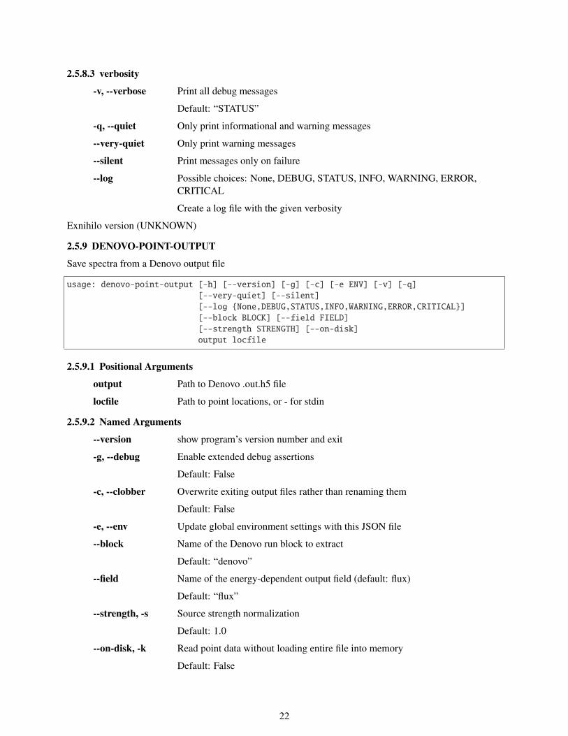
2.5.9 DENOVO-POINT-OUTPUT
Save spectra from a Denovo output file
usage: denovo-point-output [-h] [--version] [-g] [-c] [-e ENV] [-v] [-q][--very-quiet] [--silent][--log None,DEBUG,STATUS,INFO,WARNING,ERROR,CRITICAL][--block BLOCK] [--field FIELD][--strength STRENGTH] [--on-disk]output locfile
2.5.9.1 Positional Arguments
output Path to Denovo .out.h5 file
locfile Path to point locations, or - for stdin
2.5.9.2 Named Arguments
--version show program’s version number and exit
-g, --debug Enable extended debug assertions
Default: False
-c, --clobber Overwrite exiting output files rather than renaming them
Default: False
-e, --env Update global environment settings with this JSON file
--block Name of the Denovo run block to extract
Default: “denovo”
--field Name of the energy-dependent output field (default: flux)
Default: “flux”
--strength, -s Source strength normalization
Default: 1.0
--on-disk, -k Read point data without loading entire file into memory
Default: False
22

2.5.9.3 verbosity
-v, --verbose Print all debug messages
Default: “STATUS”
-q, --quiet Only print informational and warning messages
--very-quiet Only print warning messages
--silent Print messages only on failure
--log Possible choices: None, DEBUG, STATUS, INFO, WARNING, ERROR,CRITICAL
Create a log file with the given verbosity
Exnihilo version (UNKNOWN)
23


3. OMNIBUS INPUT DESCRIPTION
The Omnibus input is split into a hierarchy of blocks comprised of databases, sublists, and parameters.The front end also supports “commands” for creating or modifying input parameters, as well as additionalpre-processing and post-processing for validation.
Databases, sublists, and parameters all have the following properties:
Name The name of the parameter as it appears in the input. Some parameters have shorteraliases (e.g., nemin for n_energy_min) that appear in the documentation just below thefull parameter name.
Description The text immediately below the name should describe what it means and how it isused.
Applicable when A series of rules describing when the parameter may or may not be used.These rules take into account other parameters as well as the build configuration. Bulleted“applicability” items indicate that all the conditions must be met.
Default If present, a default value for the parameter or database. The default may be a fixedvalue (e.g., 3.0), or it may be a procedure based on the other input parameters, in whichcase a rough description of the default is given. For databases and sublists, the defaultmay appear as a Python expression (e.g., '_type': "none" for a database with type“none”). If no default is given, then the parameter or database is required in the givencontext. However, a few parameters and databases are optional and are marked accordingly.
Export The parameter will be renamed when writing to the .inp.xml file for historical reasons.
Note: This documentation was generated automatically with the following version of Exnihilo:
version 6.3.pre-b13 (branch ‘master’ on ‘upstream’, r729: #9809b44f on 2020JUL16)
date 2020-07-16 22:02:43
3.1 OMNIBUS INPUT FILE CONTENTS
Each of the top-level blocks (and the overall problem input file) are described here.
database [COMP]Composition options and definitions. See [COMP] (page 106).
Default (empty database)
database [DENOVO]Denovo solver options. See [DENOVO] (page 176).
Applicable when
• ‘Denovo’ is enabled in this build; and
• solver is ‘denovo’
database [DEPLETION]ORIGEN nuclide depletion options. See [DEPLETION] (page 212).
25

Applicable when
• ‘depletion’ is enabled in this build; and
• solver is ‘depletion’
deprecated geometryDeprecated entry geometry has been renamed to model.
Update to model
database [HYBRID]Monte Carlo acceleration method. See [HYBRID] (page 224).
Applicable when problem mode is hybrid
database [MODEL]Representation of geometry and compositions. See [MODEL] (page 43).
database [OUTPUT]Output options. See [OUTPUT] (page 39).
Default (empty database)
sublist [PHYSICS]Physics treatment. See [PHYSICS] (page 85).
Default void physics when in mode raytrace
database [POST]Post-processing options. See [POST] (page 229).
Default (empty database)
database [PRE]Pre-processing options. See [PRE] (page 227).
Default (empty database)
database [PROBLEM]Problem identifiers and mode. See [PROBLEM] (page 27).
sublist [RESPONSE]Tally responses. See [RESPONSE] (page 111).
Applicable when
• using Shift, or in adjoint mode with adjoint_source tally; and
• solver is ‘shift’
Default (empty sublist)
database [RUN]Execution parameter. See [RUN] (page 29).
Default (empty none database)
database [SHIFT]Shift Monte Carlo solver options. See [SHIFT] (page 167).
26

Applicable when
• ‘Shift’ is enabled in this build; and
• solver is ‘shift’
parameter solvers(advanced)List of solvers being used.
Default based on presence of Shift/Denovo
Type list in which each element is a string
sublist [SOURCE]Particle source definition. See [SOURCE] (page 56).
Default model-defined source if applicable, or global fission for kcode
Applicable when using Shift, in forward mode, or in adjoint mode with adjoint_sourcesource
postprocessorOnly a single ‘sourcerer’ source may be present.
Applicability solver is ‘shift’
Applicability solver is ‘denovo’
Applicability problem mode is kcode
database [TALLY]Tallies and Monte Carlo diagnostics. See [TALLY] (page 113).
Default (empty database)
Applicable when using Shift, or in adjoint mode with adjoint_source tally
3.2 PROBLEM ATTRIBUTES: [PROBLEM]
The problem database specifies top-level information about the problem being run. It includes the output filename, a unique problem identifier, and the overall solution technique.
parameter adjoint_sourceWhich block to use to construct adjoint source.
Choose whether a cell or mesh tally from the [TALLY] block or a manually defined source from the[SOURCE] block is used as an adjoint source. Currently there are a number of limitations on usingtallies as adjoint sources.
Warning: Creating an adjoint source from tallies is experimental: the adjoint source strengthand spectrum may unexpected, or the particular type of selected tally might not be implemented.Contact the developers to find out if the latest capabilities meet your needs.
Default source
Type source or tally
27

Applicable when mode is adjoint
parameter modeProblem mode.
Valid modes are:
kcode Solve the k-eigenvalue problem for criticality safety or reactor physics analysis.
forward Solve a fixed-source problem for shielding calculations, etc.
adjoint Solve an adjoint fixed-source problem with the [SOURCE] or [TALLY] block interpreted asadjoint source (see adjoint_source (page 27)). Only Denovo can run adjoint problems.
raytrace Use the Denovo ray tracer to generate discretized materials for the problem. No transportwill be performed.
hybrid Run a forward transport problem in Shift using deterministic acceleration.
Type adjoint, forward, hybrid, kcode, or raytrace
parameter nameDescriptive problem name.
Default Untitled
Type string
parameter num_threadsNumber of OpenMP threads per process.
Currently, only Shift transport supports multithreading. Denovo solution time will not be affected byincreasing the number of threads.
Default 1
Type positive integer
Applicable when ‘OpenMP’ is enabled in this build
preprocessor (advanced)Ignore manual input of pid, rev.
parameter pid(advanced)Unique identifier automatically set for this problem run.
The problem identifier (pid) is a unique string generated by the Omnibus pre-processor to ensure thatinput and output files are properly correlated. The problem ID value added to the XML input fileis copied to all HDF5 output files. It is comprised of the problem execution date and a randomlygenerated unique identifier string (UUID).
Default unique problem identifier
Type string
parameter scale_rev(advanced)SCALE source revision used to generate this file.
Default current Exnihilo revision
28

Type integer
parameter seedRandom number generator seed.
The random number generator seed is used for multiple parts of both Denovo and Shift runs:
• Shift particle sourcing and transport
• Denovo uncollided flux (if the MC option is enabled)
• Denovo material ray tracing (if not using the rays_deterministic option)
• Denovo source point sampling
Default 2272013
Type non-negative integer
3.3 EXECUTION: [RUN]
The [RUN] database enables support for running the Omnibus executable with the omnibus-run (page 15)command. The auto-run feature will format and echo program output to the screen, and it automatically savesthe output and error streams to disk.
If the SCALE and DATA environment variables are not set, omnibus-run will use the values determined atconfiguration time.
Table 3: Available types for the [RUN] database
Type Description Applicability
none (page 29) Do not run; only perform pre-processingserial (page 29) Run on a single CPU corempi (page 30) Run on multiple cores by directly calling MPI ‘MPI’ is enabled in this buildpbs (page 30) Run by submitting a PBS job ‘MPI’ is enabled in this buildcray (page 34) Run on Cray supercomputers ‘MPI’ is enabled in this buildtitan Alias to cray type —
3.3.1 [RUN=NONE]
Do not run; only perform pre-processing.
3.3.2 [RUN=SERIAL]
Run as a serial process on the local machine, echoing output to the user. If the omnibus-run process isaborted, the omnibus command will also abort.
parameter hostname(advanced)Cluster name for automatically determining processor options.
Default based on hostname or PBS_O_HOST environment
Type __unknown__, apollo, cades, eos, excalibur, falcon, falcon2, oic,poseidon2, remus, romulus, or titan
parameter omnibus(advanced)Path to the Omnibus executable.
Default '/.../omnibus'
Type file path for reading
29

3.3.3 [RUN=MPI]
Run as an MPI process on the local machine, echoing output to the user. If the omnibus-run process isaborted, the mpirun omnibus command will also abort.
parameter hostname(advanced)Cluster name for automatically determining processor options.
Default based on hostname or PBS_O_HOST environment
Type __unknown__, apollo, cades, eos, excalibur, falcon, falcon2, oic,poseidon2, remus, romulus, or titan
parameter mpiexec(advanced)Path to the MPI run command.
Default '/.../mpiexec'
Type file path for reading
parameter mpiexec_argsMPI execution arguments passed to mpiexec.
Default Based on CMake configuration and value for np
Type list in which each element is a string
parameter npNumber of processors to run.
Default PBS_NP if inside a PBS session
Type positive integer
parameter omnibus(advanced)Path to the Omnibus executable.
Default '/.../omnibus'
Type file path for reading
3.3.4 [RUN=PBS]
Create a PBS run file for this job. An example of a typical PBS run block is
[RUN=pbs]nodes 1ppn 16pmem 7900mbwalltime "24:00:00"
If the omnibus-run command is aborted while the job is run, the job will not be automatically aborted. Theqdel command must be invoked independently to abort the job.
The cpp option specifies the number of cores to be used by each MPI task: cpp 2 will use half the coresavailable on the node. Alternatively, the number of processors per node can be set using the ppn parameter.The product of these two parameters cannot exceed the number of cores available on a compute node.
Additionally, the number of total MPI tasks used to run Exnihilo can be reduced below the requested numberof nodes and cores with the np option, which has a default based on the number of requested nodes and cores.Adjusting this parameter may be necessary if, for example, Shift is to be decomposed into a non-power-of-2number of blocks.
30

parameter accountAccount number to charge for time (e.g., NFI000, NSED).
Default based on hostname
Type string
parameter attributesparameter attr
key=value pairs for PBS attributes (-W argument).
Default based on hostname
Type list in which each element is a string
parameter bindBind processes to hardware tasks.
Type boolean
postprocessorEnsure that the layout is consistent with the host cluster.
Applicability Host cluster has been detected or specified
parameter cppNumber of cores to assign to each process.
Type positive integer
parameter detachSimply submit the job and to not follow it.
Default False
Type boolean
parameter emailEmail address of recipient.
Default result of git config author.email (optional)
Type string
parameter environEnvironment variables to export in the PBS script.
Default ---
Type list of variables (each element is a string without special characters)
parameter extra_cmdsExtra commands to run at the beginning of the PBS script.
Default ---
Type list in which each element is a string
parameter holdSet jobs to ‘hold’ status when submitting.
31

Default False
Type boolean
Applicable when detach is True
parameter hostname(advanced)Cluster name for automatically determining processor options.
Default based on hostname or PBS_O_HOST environment
Type __unknown__, apollo, cades, eos, excalibur, falcon, falcon2, oic,poseidon2, remus, romulus, or titan
parameter joinOutput joining flags.
Default oe
Type string
parameter modulesModules to load at the beginning of the script execution.
Default based on hostname
Type list in which each element is a string
parameter mpiexec(advanced)Path to the MPI run command.
Default '/.../mpiexec'
Type file path for reading
parameter mpiexec_argsMPI execution arguments passed to mpiexec.
Default Based on host layout
Type list in which each element is a string
parameter nameJob name.
Default base name of problem input file
Type string without special characters
parameter node_kw(advanced)PBS keyword to specify the number of nodes.
Default usually ‘nodes_ppn,’ but ‘nodes’ on Titan and ‘select’ on others
Type nodes_ppn, nodes, or select
preprocessor (advanced)Automatically determine the layout from the host and the given arguments.
parameter nodesNumber of compute nodes to use.
32

Type positive integer
parameter npTotal number of MPI processes.
Type positive integer
parameter omnibus(advanced)Path to the Omnibus executable.
Default '/.../omnibus'
Type file path for reading
parameter pmemAmount of memory per reserved processor (e.g., ‘7900mb’).
Optional
Type string
parameter ppnNumber of processes to execute on each node.
Type positive integer
parameter projectProject name used in the -P flag.
Default based on hostname
Type string
parameter qdelPBS deletion command or path.
Default qdel
Type string
parameter qosPBS job classification option.
Default based on hostname and job specs
Type string
parameter qstatPBS status command or path.
Default qstat
Type string
parameter qsubPBS submission command or path.
Tip: To generate a PBS file but not actually submit or hold it, set qsub to “echo”, and set detachtrue. With these two options, no PBS commands will be invoked.
33

Default qsub
Type string
parameter queueparameter q
Queue to use.
Optional
Type string
parameter walltimeWall time limit.
Note: It is common to have colons as part of the wall time. Since colons must be escaped in OmnibusASCII input, the walltime input parameter will typically need escaping:
[RUN=pbs]walltime "24:00:00"
Type hh:mm:ss or mm:ss or number of seconds
parameter when_emailWhen to email.
Default ea
Type string
Applicable when Email is present
3.3.5 [RUN=CRAY]
Create a PBS file for this job to run on Cray machines. An example PBS run block is:
[RUN=cray]nodes 1024ppn 16account nfi000walltime "12:00:00"
Just like with PBS, if the omnibus-run command is aborted while the job is run, the job will not beautomatically aborted. The qdel command must be invoked independently to abort the job.
If the number of cores is less than or equal to 8 (the number of “shared core units”), the -j 2 option willautomatically be appended to stride the cores by 1.
parameter accountAccount number to charge for time (e.g., NFI000, NSED).
Default based on hostname
Type string
34

parameter aprun(advanced)Path to the aprun command.
Default '/.../mpiexec'
Type file path for reading
parameter attributesparameter attr
key=value pairs for PBS attributes (-W argument).
Default based on hostname
Type list in which each element is a string
parameter bindBind processes to hardware tasks.
Type boolean
postprocessorEnsure that the layout is consistent with the host cluster.
Applicability Host cluster has been detected or specified
parameter cppNumber of cores to assign to each process.
Type positive integer
parameter debugShow the aprun layout.
Default False
Type boolean
parameter detachSimply submit the job and to not follow it.
Default False
Type boolean
parameter emailEmail address of recipient.
Default result of git config author.email (optional)
Type string
parameter environEnvironment variables to export in the PBS script.
Default ---
Type list of variables (each element is a string without special characters)
parameter extra_cmdsExtra commands to run at the beginning of the script.
35

Default 'ulimit -c unlimited' 'export ATP_ENABLED=1'
Type list in which each element is a string
parameter holdSet jobs to ‘hold’ status when submitting.
Default False
Type boolean
Applicable when detach is True
parameter hostname(advanced)Cluster name for automatically determining processor options.
Default based on hostname or PBS_O_HOST environment
Type __unknown__, apollo, cades, eos, excalibur, falcon, falcon2, oic,poseidon2, remus, romulus, or titan
parameter joinOutput joining flags.
Default oe
Type string
parameter memMemory required per MPI task (with G/M/K extension).
Default ''
Type string
parameter modulesModules to load at the beginning of the script execution.
Default based on hostname
Type list in which each element is a string
parameter nameJob name.
Default base name of problem input file
Type string without special characters
parameter node_kw(advanced)PBS keyword to specify the number of nodes.
Default usually ‘nodes_ppn,’ but ‘nodes’ on Titan and ‘select’ on others
Type nodes_ppn, nodes, or select
preprocessor (advanced)Automatically determine the layout from the host and the given arguments.
parameter nodesNumber of compute nodes to use.
36

Type positive integer
parameter npTotal number of MPI processes.
Type positive integer
parameter omnibus(advanced)Path to the Omnibus executable.
Default '/.../omnibus'
Type file path for reading
parameter pin_systemPin system tasks to a single CPU core.
Default True if not using all cores on a node
Type boolean
Applicable when hostname is titan or eos
parameter placeHow to distribute jobs on the node.
Default 'scatter:excl'
Type string
Applicable when hostname is excalibur
parameter ppnNumber of processes to execute on each node.
Type positive integer
parameter projectProject name used in the -P flag.
Default based on hostname
Type string
parameter qdelPBS deletion command or path.
Default qdel
Type string
parameter qosPBS job classification option.
Default based on hostname and job specs
Type string
parameter qstatPBS status command or path.
Default qstat
37

Type string
parameter qsubPBS submission command or path.
Default qsub
Type string
parameter queueparameter q
Queue to use.
Optional
Type string
parameter shared_gpuAllow all processes to access GPU.
Default True when running Denovo on Titan
Type boolean
parameter tasks_per_unitNumber of processors/hwthreads to use per core unit.
Controls either the number of integer cores used per compute unit or hyperthreading.
Default based on CPUs per node
Type non-negative integer
deprecated threads_per_taskDeprecated entry threads_per_task has been renamed to cpp.
Update to cpp
parameter walltimeWall time limit.
Type hh:mm:ss or mm:ss or number of seconds
parameter when_emailWhen to email.
Default ea
Type string
Applicable when Email is present
38

3.4 OUTPUT OPTIONS: [OUTPUT]
Omnibus, Denovo, and Shift are used on a multitude of platforms and system configurations and are run atmany scales, ranging from single-CPU jobs that produce very little output to 300k-core jobs with hundredsof gigabytes of output. When large amounts of data are written to disk, the I/O performance of HDF5 (theoutput format used by Omnibus) can make a dramatic difference in write time.
Like Exnihilo, HDF5 supports both desktop and supercomputer platforms. HDF5 also supports a featurefound on many larger computational clusters: a parallel file system (PFS). Unlike a networked file system(NFS), in which a file is mirrored or mounted over a network, and updates on one computer will be seen onthe remainder of the network, a PFS actually supports writing to and reading from a file concurrently frommultiple compute nodes. An example of a PFS is Lustre, on which files are decomposed across multipleseparate hard disks. The more disks that a file is stored on, the higher the peak theoretical I/O bandwidth.
Warning: HDF5 will perform extremely poorly when writing in parallel to an NFS drive. (Factor-of-100slowdowns have been seen.) Install the psutil12 python package to allow Omnibus to detect and warnabout the file system being written to.
HDF5 can be compiled using MPI to enable “collective” operations, in which each application process canwrite a subset of the data (e.g., the locally KBA-decomposed Denovo mesh) to a file, and HDF5 will combinethe data into a single file automatically. If the HDF5 implementation being used is compiled correctly(for example, configured with --with-io-romio-flags="--with-file-system=nfs+ufs+lustre"),it will be able to interface with the parallel file system and change the file layout when a new HDF5 file iscreated.
The file layout (number of aggregators and chunk size) is system- and output-dependent; its performance13 istightly coupled to low-level HDF5 parameters, as well. Omnibus attempts to choose the output parametersfor some known systems; a lustre (page 42) command is available to change the stripe and aggregator sizeand to update the HDF5 chunk size to match.
Since parallel HDF5 is not installed on (or performant on) all systems, Exnihilo implements its own collectiveoperations for domain-decomposed data. With this “pseudo-parallel” mode, data from each domain are sentsequentially to processor 0 and then are written out using serial HDF5 calls. The disable_parallel_hdf5(page 39) option forces this alternative implementation to be enabled, even if HDF5 is available.
When parallel HDF5 is enabled (and the problem is being run on more than one process), a second outputfile with the extension -parallel.h5 will be created for collective operations. The created fields (such asDenovo flux and depletion number densities) will be linked into the main HDF5 file using the “external link”feature of HDF5, so only the main .h5 file should ever need to be opened, although both files will need to beretained.
parameter disable_parallel_hdf5(advanced)Disable MPI-I/O and write only from a single process.
Default True unless the file system is parallel
Type boolean
Applicable when ‘PARALLEL_HDF5’ is enabled in this build
12 http://pythonhosted.org/psutil/13 https://support.hdfgroup.org/pubs/papers/howison_hdf5_lustre_iasds2010.pdf
39

postprocessorDisallow parallel HDF5 compatibility with non-PFS.
Applicability ‘PARALLEL_HDF5’ is enabled in this build; disable_parallel_hdf5is False; and the problem run is parallel
Applicability file_system is __unknown__, nfs, nfs3, nfs4, hfs, ntfs, ext3, ext4,tmpfs, sysfs, btrfs, hugetlbfs, apfs, or xfs
parameter display_counter(advanced)Write terminal commands for an interactive counter.
Default True if stderr is a terminal display
Type boolean
Applicable when The ‘tqdm’ python package is installed
parameter file_system(advanced)parameter fs(advanced)
File system type where output is being written.
Default Based on output of the mount command
Type __unknown__, __parallel__, lustre, panasys, nfs, nfs3, nfs4, hfs, ntfs,ext3, ext4, tmpfs, sysfs, btrfs, hugetlbfs, apfs, or xfs
postprocessorDisallow NFS output if a PFS is available.
Applicability ‘PARALLEL_HDF5’ is enabled in this build
Applicability the problem run is parallel
Applicability file_system is __unknown__, nfs, nfs3, nfs4, hfs, ntfs, ext3, ext4,tmpfs, sysfs, btrfs, hugetlbfs, apfs, or xfs
parameter hdf5_alignment(advanced)Alignment threshold and alignment value for HDF5.
Default 0 0
Units B
Type list in which each element is a non-negative integer
Applicable when
• ‘PARALLEL_HDF5’ is enabled in this build; and
• disable_parallel_hdf5 is False; and
• the problem run is parallel
parameter hdf5_chunk(advanced)Target size of HDF5 chunks; chunks will be this size or smaller.
Default 65536
Units B
40

Type positive integer
preprocessor (advanced)Set default Lustre striping based on hostname.
Applicability ‘PARALLEL_HDF5’ is enabled in this build
Applicability disable_parallel_hdf5 is False
Applicability the problem run is parallel
parameter hdf5_mpiinfo_key(advanced)MPI_Info keys for parallel HDF5 file creation.
Default ---
Type list in which each element is a string
Applicable when
• ‘PARALLEL_HDF5’ is enabled in this build; and
• disable_parallel_hdf5 is False; and
• the problem run is parallel
parameter hdf5_mpiinfo_value(advanced)MPI_Info values for parallel HDF5 file creation.
Default ---
Type list in which each element is a string
Applicable when
• ‘PARALLEL_HDF5’ is enabled in this build; and
• disable_parallel_hdf5 is False; and
• the problem run is parallel
postprocessorThe parameters hdf5_mpiinfo_key and hdf5_mpiinfo_value must have the same length.
Applicability ‘PARALLEL_HDF5’ is enabled in this build
Applicability disable_parallel_hdf5 is False
Applicability the problem run is parallel
parameter log_memory(advanced)Periodically print memory usage to screen.
Default True if using Denovo
Type boolean
parameter log_timestampPrepend a timestamp with this format to each log message.
The formatting for a time stamp is the standard strftime14 formatting. For example, a value of[%H:%M:%S] may produce a log message that looks like:
14 https://en.cppreference.com/w/cpp/chrono/c/strftime
41

>>> [11:29:43] Time-stamped message
Optional
Type string
parameter log_verbosityMinimum level of output to save to log file.
Default info
Type debug, diagnostic, status, info, warning, error, or critical
command lustreSet stripe size, aggregator, and HDF5 chunk size [kB, #].
Creates hdf5_mpiinfo_key
Creates hdf5_mpiinfo_value
Creates hdf5_alignment
Creates hdf5_chunk
Applicable when file_system is __unknown__, __parallel__, lustre, or panasys
parameter output(advanced)Destination path for the HDF5 output file.
Default input.out.h5
Type file path to write (extension ‘.h5’)
parameter output_parallel(advanced)Destination path for parallel HDF5 output.
Default input.out-parallel.h5
Type file path to write (extension ‘.h5’)
Applicable when
• ‘PARALLEL_HDF5’ is enabled in this build; and
• disable_parallel_hdf5 is False; and
• the problem run is parallel
deprecated print_memoryDeprecated entry print_memory has been renamed to log_memory.
Update to log_memory
parameter screen_verbosityMinimum level of output to print to screen.
Default diagnostic
Type debug, diagnostic, status, info, warning, error, or critical
42

3.5 MODEL DEFINITION: [MODEL]
We define a model as the answer to the question: “What is where?” A model can include compositions,spatial geometry, and even sources and tallies. As a radiation transport framework, Exnihilo supports modeldefinitions in several formats.
Every model contains a geometry that can be discretized and solved using Denovo with the built-in ray tracer,and most models can also be used by the Shift Monte Carlo code. Furthermore, material definitions can beconverted to multigroup cross sections through the SCALE cross section processing libraries or mixed intomultigroup cross sections input in ANISN formats.
Table 4: Feature matrix for the supported models.
Model Denovo Shift Compositions Sources Tallies
DAGMC Yes Yes — — —Geant4 Yes No Yes — —Geometria Yes Yes — — —MCNP Yes Yes Yes Yes NoMesh Yes Yes — Yes —RTK Yes Yes — — —SCALE Yes Yes Yes No NoSWORD Yes No Yes Yes YesVERA Yes Yes — — —
If using Shift to obtain volume-averaged reaction rates in geometric cells, the volume of the cells must beobtained a priori. Some models support automatic calculation a subset of cells; only Reactor ToolKit input:[MODEL=rtk] (page 53) supports automatic calculation of all cell volumes due to the restricted simple natureof the geometry. For all other models, the cell volumes can be manually specified with the “volumes” and“volume_cells” keywords:
volumes 1.0 2.34 0.5volume_cells 1 200 15
Here, the cells are the “cell labels” (e.g., the cell card IDs in MCNP) and the volumes are the correspondingvolumes in cm3. The volumes are used only in the normalization of tallies, including depletion tallies.
3.5.1 MATERIAL AND CELL IDS
The model internally defines vectors of “matids” and “cellids” that correspond to user-defined materialnames and cell labels. Although Omnibus attempts to make these internal identifiers invisible to the user, anoccasional advanced option or low-level error message may include references to these.
The material ID is simply the index into the list of compositions (page 106) in the problem; these are writtento the comp/compositions dataset in the Omnibus output file. Note that for the MCNP model (page 44),these are usually not the user-assigned m label.
Cell IDs correspond to identifiable user-created spatial regions in the problem. If arrays or universes are used,a single cell ID might correspond to multiple regions in space. Cell IDs are not written to the output filebecause
• cells are typically much more numerous than materials;
43

• some models such as RTK do not have user-provided identifiers for cells; and
• some models such as Geometria reserve cell IDs as implementation details, so some cell IDs correspondto no physical point in space.
User-provided labels corresponding to cell and material IDs can both be obtained without having to run theOmnibus executable. The following snippet uses the Python bindings (page 2) to print the meanings of allmatids and cellids in the model:
from omnibus.raytrace.load import load_mcnpmodel = load_mcnp('ueki.runtpe')print("Materials:")print("\n".join(" :3d -> :s".format(c.compid, c.name)
for c in model.compositions))print("Cells:")print("\n".join(" :3d -> :s".format(i, geo.cell_to_label(i))
for i in range(geo.num_cells)))
Table 5: Available types for the [MODEL] database
Type Description Applicability
mcnp (page 44) MCNP model definition ‘Lava’ is enabled in this buildscale (page 50) SCALE KENO input file ‘SCALE_GEO’ is enabled in this buildgeometria (page 52) Geometria input definition ‘GG’ is enabled in this buildgg Alias to geometria type —rtk (page 53) RTK input specificationmesh (page 53) Explicit meshed problem in HDF5 format ‘HDF5’ is enabled in this buildgeant (page 54) Geant4 GDML model input ‘Geant’ is enabled in this buildsword (page 54) SWORD model description ‘SWORD’ is enabled in this builddagmc (page 55) DAGMC CAD geometry definition ‘DAGMC’ is enabled in this buildvera (page 56) VERA input specification ‘VERA’ is enabled in this build
3.6 MCNP INPUT: [MODEL=MCNP]
Exnihilo supports reading MCNP [18] input files through ORNL’s Lava library [7]. The user’s MCNP inputfile must be processed through MCNP using the mcnp5 ix inp=inp command in order to generate theruntpe file that Lava requires. The Omnibus pre-processor does this automatically.
Note: If using Shift cell tallies with an MCNP model, the user must include a cell tally or input volumes fordesired cells in the MCNP input to ensure that volumes to automatically be propagated into Shift.
3.6.1 FEATURES
• Any MCNP5-compatible geometry is supported.
• MT cards for the materials are automatically converted to their equivalent SCALE IDs, so for example6000 with a corresponding grph card will be converted to the SCALE ID for graphite, 3006000.
• In depletion calculations, groups of axis-aligned planes can be moved at each time step withoutrestarting (see [MODEL][MOVABLE=surfaces] (page 50))
• SDEF sources can be transported with Shift using the [SOURCE=mcnp] (page 61) source definition.
44

3.6.2 LIMITATIONS
• MCNP6 is not supported; MCNPX will not be supported.
• Library suffixes for nuclides in the material block are ignored: only the TMP (temperature) card on eachcell is used to determine the composition temperature. The composition temperature is then used whenloading CE nuclides.
• Tally definitions are ignored.
• MCNP sources cannot be automatically biased in hybrid modes.
• Only MT cards natively supported by MCNP5 will be interpreted as chemically bound elements.
3.6.3 NAMING
Geometry cell names are the same as the numerical cell “names” given in the cell block of the MCNP input.Unlike MCNP, which can tally a single instance of a cell that is present in different arrays or universes with aspecial input such as 2>4>1, Shift will lump all instances of a cell into the same tally.
Most material compositions processed from MCNP have the form mNNN, where NNN is the material namespecified on the m card. However, if the material is present in the cell definition block at multiple densitiesand/or temperatures, multiple copies of the composition will be present. Lower-density compositions willhave the form mNNN (FF.F%), where FF.F is the percentage mass density compared to the highest-densityinstance of the material.
3.6.4 NUCLIDE MAPPING
Exnihilo implements a number of hard-coded mappings to convert both bound and unbound MCNP nuclidesto their equivalent IDs in SCALE. The following translations are performed for unbound nuclides:
Table 6: Mappings between unusual nuclide IDs.
MCNP ID SCALE ID
1001 80010011002 800100227458 102705847510 104711048515 104811552527 105212752529 105212961548 106114867566 106716695642 9524295242 109524295644 1095244
The MT cards in MCNP input mark that atoms in the material are chemically bound, so a S (α, β) collisionkernel for thermal energies is to be applied. In SCALE, individual nuclides are marked as having boundcollision data, so the following nuclides in bound materials in MCNP are translated to special SCALE IDs:
45

Table 7: Mappings between MCNP MT cards and SCALE IDs.
MTn ZAID SCALE ID
al27 13027 1013027be 4009 3004009be/o 4009 5004009benz 1001 6001001
6000 50060006012 5006000
beo 4009 30040098016 8016
dortho 1002 4001002dpara 1002 5001002fe56 26056 1026000grph 6000 3006000
6012 3006000h/zr 1001 7001001hortho 1001 4001001hpara 1001 5001001hwtr 1002 1002lmeth 1001 1001001lwtr 1001 1001o/be 8016 5008016
8017 80178018 8018
o2/u 8016 10080168017 80178018 8018
poly 1001 9001001sio2 14028 1014028
14029 101402914030 1014030
smeth 1001 2001001u/o2 92238 92238zr/h 40000 1040090
40090 104009040091 104009140092 104009240094 104009440096 1040096
command autonameAttempt to provide MCNP material names using their compositions.
The autoname command is an experimental tool that loads the MCNP runtpe file into memory usingthe Exnihilo Python bindings (page 2) and uses the MCNP-defined compositions to construct a “bestguess” of their name based on their most abundant elements.
46

Tip: After autoname has been run once, a user can extract the created names from the PROBLEM.inp.omn file created in the run directory, replace the autoname command with those names, and modifythem as desired.
Creates mat_names
Creates mat_name_mno
parameter cell_raytraceTransform cell labels into material IDs for raytracing.
Default False
Type boolean
Applicable when problem mode is raytrace
parameter extentsBounding box for the active region of the geometry.
Setting the model boundary enables certain Exnihilo features that require “global” boundaries. Theseinclude:
• Global mesh tallies
• Global initial fission source
• Automatic Shannon entropy mesh
• MCNP source discretization for Denovo
Default -1e+100 1e+100 -1e+100 1e+100 -1e+100 1e+100
Type locations for -X,+X,-Y,+Y,-Z,+Z (each element is a real number)
command inputGenerate an MCNP runtpe file and set runtpe_path.
This command uses the version of MCNP configured with Exnihilo to generate a run tape. To changethe cross section lookup directory xsdir, set the environment variable DATAPATH before running theOmnibus pre-processor. An informational message will acknowledge that the environment variable isbeing used in the particular MCNP run.
Tip: The MCNP executable path can be overridden by modifying the execution environment with the-e env.json argument to omnibus-run (page 15). Use a JSON environment file that looks like
"cmake": "MCNP_EXECUTABLE": "/path/to/mcnp5"
Creates runtpe_path
47

command mMap ‘mat_name_mno’ to ‘mat_names’ from pairs or arrow-separated items.
Creates mat_name_mno
Creates mat_names
parameter mat_name_mnoMCNP material ‘names’ corresponding to the given mat_name override.
Default ---
Type Integer material numbers in MCNP (each element is a positive integer (optionalleading ‘m’))
postprocessorThe parameters mat_names and mat_name_mno must have the same length.
parameter mat_namesparameter mat_name
Override names for materials in the geometry.
Custom names can be added to the model that will be reflected in material plots inside VisIT and insidepost-processing data elements. MCNP material card numbers are specified alongside new names touse:
mat_name_mno :mat_names1 "sodium iodide"2 "carbon steel"13 polyethylene14 iron105 air106 concrete
Default ---
Type list in which each element is a non-empty string
sublist [MOVABLE]Geometry elements that can be modified during the simulation. See [MODEL][MOVABLE] (page 49).
Default (empty sublist)
database [RAYTRACE]Volume calculation. See [MODEL][RAYTRACE] (page 49).
Optional
Applicable when problem mode is raytrace
parameter runtpe_path(advanced)Path to the MCNP runtpe file.
Type file path for reading
parameter volume_cellsCell labels corresponding to the given volume overrides.
48

Default ---
Type list of cell labels (each element is a string)
postprocessorThe parameters volumes and volume_cells must have the same length.
parameter volumesProvide or override volumes for cells in the geometry.
Default ---
Units cm3
Type list in which each element is a positive real number
3.6.5 [MODEL][MOVABLE]
Table 8: Available types for the [MOVABLE] database
Type Description Applicability
surfaces (page 50) Movable surface group
3.6.6 [MODEL][RAYTRACE]
Volume calculation.
parameter axesAxis/axes along which to fire rays for ray trace.
Default xyz
Type axis or axes (‘x’,’zy’,’xyz’)
parameter error_toleranceFraction of lost rays to tolerate before aborting.
Default 1e-05
Type real number inside (0, 1)
parameter max_local_warningsMax number of lost ray warnings to print per domain.
Default 10
Type non-negative integer
parameter num_batchesNumber of batches to use for estimating variance.
Default 8
Type positive integer
parameter ray_spacingAverage spacing between rays in each batch.
Units cm3
49

Type positive real number
parameter rays_deterministicUse face midpoints rather than stratified sampling.
Default False
Type boolean
parameter traceWhether to trace materials or cell volumes.
Default cell
Type mat or cell
3.6.7 [MODEL][MOVABLE=SURFACES]
The “movable” surface option allows the translation of multiple surfaces simultaneously in the MCNP model.Currently this works only for simple axis-aligned planes.
Warning: Because translations and surface deduplication are applied while generating the runtpe file,moving one surface label may end up affecting other coincident surfaces. Exnihilo will raise an errorduring setup if this happens: the input deck will need to be modified to remove coincident planes orinclude all equivalent (coincident) surfaces in the surface group specification.
parameter initialMovement to apply before the first transport.
Default 0.0
Units cm
Type real number
parameter nameName of the surface group.
Type string without special characters
parameter surfacesList of MCNP surface labels to move over time.
Type list in which each element is a positive integer
3.7 SCALE INPUT: [MODEL=SCALE]
As an alternative to SCALE’s CSAS-Shift sequence, the geometry and composition definitions from a SCALEinput file can be processed and run through Omnibus. Any valid SCALE sequence inputs with a singleGEOMETRY and COMPOSITION blocks can be transported on automatically.
Details on defining SCALE geometry inputs may be found in the SCALE manual [2].
3.7.1 FEATURES
• Supports KENO-V.a and KENO-VI geometry definitions, including geometries defined as part of asequence (such as MAVRIC or CSAS-Shift).
• Supports all standard composition definitions.
50

3.7.2 LIMITATIONS• Only the GEOMETRY and COMP data blocks from the SCALE input will be used. The sequence
itself is ignored, as are all other blocks (such as parameters and plotting inputs). This includes crosssection processing blocks: see Multigroup physics: [PHYSICS=mg] (page 96) for specifying thephysics treatment through Omnibus.
• Only the first one of each of those blocks will be used. If multiple sequences are chained together inthe input, all but the first will be ignored.
If no composition block is present, then the user must specify compositions separately; this advanced usecase is outside the scope of the manual.
3.7.3 NAMINGFor KENO-VI geometries, cell names take the form unit.instance, where “unit” is the integer unit number,and “instance” is the index of the media instance in the list of media for that unit.
Composition names are saved as media N, where N is the media number specified in the composition block.
3.7.4 GEOMETRY CONVENTIONSThe legacy geometry implementation in KENO differs from the new Geometria-powered implementation,which leads to confusingly different conventions that will hopefully be resolved. Until then, some of thedifferences are sketched out here.
• A universe in Geometria generally corresponds to a unit in SCALE. However, each instance of an arrayplaced as a hole (in KENO-VI) is also a universe.
• Numbering in Geometria generally uses zero-based indexing, so the lower-left element in an array hascoordinates [0 0 0] in the output.
• The “sense” of a surface or shape in Geometria generally takes the opposite sign of an input in a KENOregion definition vector. See the [UNIVERSE][CELL] (page 244) section for more details.
parameter inputPath to the KENO VI input file.
Type file path for reading (extension ‘.inp’)
database [RAYTRACE]Volume calculation. See [MODEL][RAYTRACE] (page 49).
OptionalApplicable when problem mode is raytrace
parameter volume_cellsCell labels corresponding to the given volume overrides.
Default ---
Type list of cell labels (each element is a string)
postprocessorThe parameters volumes and volume_cells must have the same length.
parameter volumesProvide or override volumes for cells in the geometry.
Default ---
Units cm3
Type list in which each element is a positive real number
51

3.8 GEOMETRIA INPUT: [MODEL=GEOMETRIA]
The Geometria (internally designated “GG”) geometry engine underpins the new SCALE geometry imple-mentation. Geometria supports a less automatic but more rigorous geometry definition than KENO. Its inputis an Omnibus-style problem definition (see Geometria Input Description (page 233)) that is translated to anXML file.
This input model only supports geometry definitions; compositions must be input either via an HDF5 inputfile or in a [COMP] block (page 106).
command inputGenerate a Geometria XML representation from an .gg.omn input.
Creates xml_path
database [RAYTRACE]Volume calculation. See [MODEL][RAYTRACE] (page 49).
Optional
Applicable when problem mode is raytrace
parameter simplify_max_surfaces(advanced)Threshold for making a “complex” cell “simple.”
In the GG implementation, a “simple” cell is a cell in which crossing a boundary always causes aparticle to leave a cell. (An example of a simple cell is the moderator region inside a square and outsidea circle.) Some cells, however, have internal surface boundaries that can be crossed while remaininginside the cell. (An example of a “complex” cell is a square region with two non-overlapping squaresexcluded. Crossing one of the inner planes that comprise the squares does not necessarily put theparticle inside the inner squares.) The bookkeeping for a particle inside these cells is more complicatedthan the simple cell, because all the distances along the particle’s path must be calculated and tracked,and every surface crossing requires the cell’s logic expression to be reevaluated to determine whetherthe particle is inside.
If a complex cell is erroneously treated as simple, tracking errors will result; so it is necessary tobe conservative in initially calling a cell complex. In GG, a cell is assumed complex if it containsa “positive” shape in its definition (i.e., it is the “outside” of a shape). This has the unfortunateconsequence of forcing the assumption that common simple shapes, such as a pin inside a pin cell, arein fact complex. The solution is a piece of code that checks a cell at construction time. It loops over allcombinations of the surface IDs connected to the cell to determine if any surface crossing will allow aparticle inside the cell to remain inside the cell:
• Fill the “surface sense” vector with the next combination of bits
• If the logic expression evaluates to “false,” skip this iteration
• Loop over every surface sense
– Flip this surface’s sense
– If the cell logic expression still evaluates to “true,” the cell is definitely complex. Returnearly.
– Restore the flipped sense
52

The performance of the above loop scales exponentially with the number of surfaces connected to acell. (If the cell only has two surfaces, 4 outer logic evaluations must be made; for four surfaces, 16must be made; for ten surfaces, 1024 must be made.) Therefore, this parameter defaults to checkingonly cells composed of at most 10 surfaces. Testing results show that this has a negligible build-timepenalty but can improve tracking time by almost a factor of two, as in the case of the C5G7 benchmark,in which each pin cell would be marked “complex” without this code.
Default 10
Type integer in the range [0,16)
parameter volume_cellsCell labels corresponding to the given volume overrides.
Default ---
Type list of cell labels (each element is a string)
postprocessorThe parameters volumes and volume_cells must have the same length.
parameter volumesProvide or override volumes for cells in the geometry.
Default ---
Units cm3
Type list in which each element is a positive real number
parameter xml_path(advanced)Path to the GG geometry XML input file.
Type file path for reading (extension ‘.xml’)
3.9 REACTOR TOOLKIT INPUT: [MODEL=RTK]RTK is an internal geometry engine used for PWR geometry under the VERA framework produced by CASL.The RTK model implemented by Omnibus reads a geometry from an XML input file. In general, the Insilicofront-end should be used for creating reactors with RTK geometries.
parameter inputPath to the RTK geometry XML or HDF5 file.
Type file path for reading (extension ‘.xml’ or ‘.h5’)
3.10 BRICK MESH INPUT: [MODEL=MESH]The “mesh” model type allows a discretized problem to be transported on in Denovo and Shift. It is definedby an external HDF5 file with a field of materials, mixtures, and (optionally) a source description. The fileformat’s specification is described in HDF5 Mesh Model Specification (page B–4)
This file format is primarily intended for Denovo problems, both for analytical benchmarks and allowing theuser to “restart” from a previously discretized geometry using the make-denovo-model (page 21) utility. Shiftdoes not support mix tables or the source description.
parameter inputPath to the mesh geometry hdf5 file.
Type file path for reading (extension ‘.h5’)
postprocessorCheck that the mesh model is in the correct format.
53

3.11 GEANT4 INPUT: [MODEL=GEANT]
Exnihilo supports Geant4 [15] inputs stored as GDML files. The materials and geometry are both readthrough Exnihilo.
Caution: Because Geant4 defines a number of nuclides that may be important to high-energy physicsbut that are not important to neutronics calculations, it may be necessary to use the omit_zaid andorig_zaid/subs_zaid options in the physics if those nuclides are not present on the cross sectionlibraries.
3.11.1 LIMITATIONS
• Tracking particles in Shift is not supported. Currently, Geant4 can only be discretized in Denovo orray-traced in Python.
parameter inputPath to the Geant4 GDML input file.
Type file path for reading (extension ‘.gdml’)
database [RAYTRACE]Volume calculation. See [MODEL][RAYTRACE] (page 49).
Optional
Applicable when problem mode is raytrace
parameter volume_cellsCell labels corresponding to the given volume overrides.
Default ---
Type list of cell labels (each element is a string)
postprocessorThe parameters volumes and volume_cells must have the same length.
parameter volumesProvide or override volumes for cells in the geometry.
Default ---
Units cm3
Type list in which each element is a positive real number
3.12 SWORD INPUT: [MODEL=SWORD]
The SoftWare for Optimization of Radiation Detectors [8] interface requires files generated by the release(non-beta) version of SWORD 6.0 or higher, as only new versions write the problem’s geometry and materialdefinitions as Geant4 GDML files.
In addition to the geometry and material definitions, the SWORD model supports source definitions using[SOURCE=sword] (page 62) and can construct adjoint sources (tallies) using [TALLY][SWORD] (page 141).
54

3.12.1 LIMITATIONS
• Since SWORD’s tracking engine is based on that of Geant (page 54), tracking particles in Shift is notsupported. Only Denovo discretization and raytracing are supported.
command inputGenerate a binary SWORD representation from a .sword input.
Creates xdr_path
parameter xdr_path(advanced)Path to the SWORD binary input file.
Type file path for reading (extension ‘.xdr’)
3.13 DAGMC INPUT: [MODEL=DAGMC]
Direct Accelerated Geometry Monte Carlo (DAGMC) is a package in MOAB that has been integrated intoExnihilo to support CAD-based models. This package allows for Monte Carlo transport on complex 3Dgeometries that have been created by traditional solid modeling software. The model must be pre-processedso that the geometry is a faceted HDF5 file, and volumes must be tagged with specific properties.
Table 9: MOAB volume properties used in the DAGMC model.
Name Description
mat Material ID (must be an integer), or the value “graveyard”.label Cell label, ignored for the graveyard volume.implicit_mat Specified only in the graveyard cell, the matid that will be
given to cells marked as implicit complements.
There can only be a single graveyard cell, which will be given the cell label “EXTERIOR,” and there can bemultiple implicit complements, which all share the label “IMPLICIT_COMPLEMENT”.
3.13.1 FEATURES
• Any faceted CAD geometry of varying complexity can be used.
• Reflecting boundaries are supported.
3.13.2 LIMITATIONS
• Labeling materials by name is not supported. Volumes in the geometry must be tagged with thecorresponding material ID.
• Volumes without material labels will be given a matid of 0.
• The extents of the geometry must be an axis-aligned rectangular prism.
parameter inputPath to the MOAB facet file.
Type file path for reading (extension ‘.h5m’)
parameter mat_inputPath to the material composition file.
55

Optional
Type file path for reading (extension ‘.h5’)
database [RAYTRACE]Volume calculation. See [MODEL][RAYTRACE] (page 49).
Optional
Applicable when problem mode is raytrace
parameter volume_cellsCell labels corresponding to the given volume overrides.
Default ---
Type list of cell labels (each element is a string)
postprocessorThe parameters volumes and volume_cells must have the same length.
parameter volumesProvide or override volumes for cells in the geometry.
Default ---
Units cm3
Type list in which each element is a positive real number
3.14 VERA INPUT: [MODEL=VERA]
The model for a Virtual Environment for Reactor Applications (VERA) [9] XML input can be run throughthe Omnibus front end. The material compositions will be built from the model. Since the VERA geometrycan only describe the geometry from the core out through the reactor vessel, the VERA input allows foran Omnibus input file defining the ex-core geometry to be specified. If this ex-core file is given, it will beincluded in the built geometry.
The [TALLY][VERA] (page 134) can be used to create a tally for the outermost region of the vessel. Thistally can then be optimized for when running in hybrid mode.
parameter inputPath to the VERA XML input file.
Type file path for reading (extension ‘.xml’)
3.15 PARTICLE SOURCE DEFINITIONS: [SOURCE]
The source database specifies the source particle distribution for a fixed-source problem, as well as the startingsource for an eigenvalue problem. Any combination of types is allowed.
The total strength of all sources is used as a global multiplier for all tallies in fixed-source mode. (The totalstrength is ignored for the starting source in kcode mode; only the relative strengths of the sources are used.)An alternative to modifying the total source strength is to modify the normalization property of the tallies.
If using Shift with mode kcode, and no source is provided, the default source is a uniform source with globalextents isotropically emitting neutrons with a U-235 watt spectrum. Since some geometry types cannot
56

determine global extents by default (e.g., MCNP requires an extents keyword), be warned that this defaultmay fail to sample enough particles in fissionable regions.
Table 10: Available types for the [SOURCE] database
Type Description Applicability
separable(page 57)
Source separable in space, energy, an-gle
fissionmesh(page 59)
Fixed fission source from a Shift tallyor mesh source
mesh (page 61) Discretized source from the meshmodel HDF5 file
model is ‘mesh’ and solver is ‘denovo’
mcnp (page 61) Source from MCNP SDEF cards model is ‘mcnp’sword (page 62) SWORD source/spectra definitions model is ‘sword’material (page 63) Volumetric material composition emis-
sionsurface_census(page 64)
Emit particles from a pre-computed sur-face source
sourcerer(page 65)
Use a Denovo solution as a fissionsource
solver is ‘shift’; solver is ‘denovo’; andproblem mode is kcode
3.15.1 [SOURCE=SEPARABLE]
Exnihilo views the source particle type as being an extension of the energy phase space. This facilitates hybridmethods, since in deterministic solvers the neutron and photon groups are adjacent and treated identically,and it makes some source definitions (such as naturally emitting materials) more straightforward.
parameter allow_biasingEnable source biasing for hybrid problem modes.
Default False
Type boolean
database [ANGLE]Particle angular distribution. See [SOURCE][ANGLE] (page 66).
Default (empty isotropic database)
parameter biased_distribution_sample_attempts(advanced)Number of distribution sampling attempts before abandoning the current cell/group phase space.
Default 1000000
Type positive integer
parameter biased_src_sample_attempts(advanced)Number of sampling attempts of a biased source before declaring a particle lost.
Default 10
Type positive integer
parameter cell_only
57

parameter cellEmit particles only in the given cells.
The cell_only criteria can be used in conjunction with fissionable_only and material_only,where it is combined using an and operation (i.e., emit particles in the given cells and in the givenmaterials).
Optional
Type list in which each element is a string
parameter descriptionparameter desc
Optional longer descriptive string.
Default ''
Type string
database [ENERGY]Energy spectrum. See [SOURCE][ENERGY] (page 66).
Default Watt spectrum when in ‘kcode’ mode
parameter fissionable_onlyparameter fis
Emit particles only in fissionable regions.
The fissionable_only criteria can be used in conjunction with material_only and cell_only,where it is combined using an and operation (i.e., emit particles in fissionable materials and in thegiven cells).
Default True if ‘kcode’ mode
Type boolean
parameter l2_errorMaximum requested source discretization L2 error.
Default 0.01
Type real number inside (0, 1)
Applicable when using Denovo or hybrid
parameter material_onlyparameter mat
Emit particles only in the given materials.
The material_only criteria can be used in conjunction with fissionable_only and cell_only,where it is combined using an and operation (i.e., emit particles in the given materials and in the givencells).
Optional
Type list in which each element is a non-empty string
parameter max_samplesMaximum number of point samples to use for discretization.
58

Default 10000000000.0
Type positive integer
Applicable when using Denovo or hybrid
parameter nameShort title or label for the source.
Default type of the source database
Type string without special characters
parameter num_rejection_samplesparameter rej
How many samples to try before declaring a particle ‘lost.’
Default 50000
Type positive integer
parameter samples_per_batchparameter batch_samples
Number of point samples per discretization batch.
Default 100000.0
Type positive integer
Applicable when using Denovo or hybrid
database [SHAPE]Spatial distribution type. See [SOURCE][SHAPE] (page 66).
parameter strengthparameter q
Source strength.
Default 1.0
Units particles
Type positive real number
3.15.2 [SOURCE=FISSIONMESH]
The fission mesh source allows a fission neutron production mesh tally from a prior run (kcode or fixedsource) to be used as a source. This source could either be a starting source in a kcode calculation (to reducethe number of inactive cycles needed) or a fixed source (so that a coupled neutron-gamma problem can berun separately from the kcode calculation). The input parameter points to the name of the tallies.h5 file;and the mesh_tally_name parameter should be the name of the fission mesh tally.
By default, this source uses a U-235 energy spectrum.
parameter allow_biasingEnable source biasing for hybrid problem modes.
Default False
Type boolean
59

parameter biased_distribution_sample_attempts(advanced)Number of distribution sampling attempts before abandoning the current cell/group phase space.
Default 1000000
Type positive integer
parameter biased_src_sample_attempts(advanced)Number of sampling attempts of a biased source before declaring a particle lost.
Default 10
Type positive integer
parameter cell_averagedparameter avg
Whether the field values are volume-averaged strengths.
Type boolean
Applicable when format is source
parameter descriptionparameter desc
Optional longer descriptive string.
Default ''
Type string
preprocessor (advanced)Default energy spectrum is U-235 Watt spectrum.
database [ENERGY]Energy spectrum. See [SOURCE][ENERGY] (page 66).
Default Watt spectrum when in ‘kcode’ mode
parameter fieldPath to the source definition in the input file.
Default ‘strength’ if cell-averaged, else ‘pdf’
Type string
Applicable when format is source
parameter formatFormat of hdf5 file.
Default tally
Type source or tally
parameter inputName of file containing source distribution.
Type file path for reading (extension ‘.h5’)
parameter nameShort title or label for the source.
60

Default type of the source database
Type string without special characters
parameter num_rejection_samplesparameter rej
How many samples to try before declaring a particle ‘lost.’
Default 50000
Type positive integer
parameter strengthparameter q
Source strength.
Default 1.0
Units particles
Type positive real number
parameter tally_nameName of the fission source rate mesh tally.
Type string without special characters
Applicable when format is tally
3.15.3 [SOURCE=MESH]
This “mesh” source is specifically for manually constructed Denovo source strengths and multigroup spectra.To use a field of source strengths in Shift, use the mesh shape (page 76) as part of a separable source.
parameter descriptionparameter desc
Optional longer descriptive string.
Default ''
Type string
parameter nameShort title or label for the source.
Default type of the source database
Type string without special characters
3.15.4 [SOURCE=MCNP]
The MCNP source uses the Lava library to extract and use the source definition from an SDEF card. It supportsautomatic interpretation of the particle type (defaulting to the problem mode) and the strength (from the WGTparameter) as well as the actual distributions themselves.
The MCNP biasing parameters will be respected when sampling this source. This also applies to creating adiscrete Denovo source from an MCNP source: regions where the source is biased to emit more frequentlywill have better statistical estimates of the source. The weight is accounted for during discretization to ensurethat the total source strength is correct as the number of source samples approaches infinity.
61

It is important to note that currently the MCNP source is replicated across processors when discretizing. Thismeans that MCNP sources that encompass many cells, especially with a fine-group energy structure, mayrequire more memory than an individual CPU core can allocate.
Note: Currently, the MCNP source is only available if the MCNP geometry is being used.
parameter descriptionparameter desc
Optional longer descriptive string.
Default ''
Type string
parameter extentsOptional bounding box for MCNP source.
To allow for an MCNP source to be discretized in parallel, it is necessary to replicate the spatial meshthat overlaps the source. By default, this option replicates the entire spatial mesh. On large problems,fully replicating the entire mesh may cause the program to abort for lack of memory.
The solution is to manually define an axis-aligned bounding box that encloses the source region. Thusonly the part of the mesh containing the source is replicated.
Tip: When the source discretization takes place, an informational message will print the ‘actual’extents (based on sample particles) of the source bounding box. If the source boundaries are not readilyavailable, it may be sufficient to discretize the source on a few-cell mesh problem and use the sampledextents (expanded by some fraction) as the bounding box for the full problem run.
Default -1e+100 1e+100 -1e+100 1e+100 -1e+100 1e+100
Type locations for -X,+X,-Y,+Y,-Z,+Z (each element is a real number)
parameter nameShort title or label for the source.
Default type of the source database
Type string without special characters
3.15.5 [SOURCE=SWORD]
This source option imports source descriptions from the SWORD input model. Currently, it only works withDenovo and is incompatible with other source definitions.
parameter allow_biasingEnable source biasing for hybrid problem modes.
Default False
Type boolean
parameter biased_distribution_sample_attempts(advanced)Number of distribution sampling attempts before abandoning the current cell/group phase space.
62

Default 1000000
Type positive integer
parameter biased_src_sample_attempts(advanced)Number of sampling attempts of a biased source before declaring a particle lost.
Default 10
Type positive integer
parameter descriptionparameter desc
Optional longer descriptive string.
Default ''
Type string
parameter nameShort title or label for the source.
Default type of the source database
Type string without special characters
3.15.6 [SOURCE=MATERIAL]
Volumetric material composition emission.
parameter allow_biasingEnable source biasing for hybrid problem modes.
Default False
Type boolean
parameter biased_distribution_sample_attempts(advanced)Number of distribution sampling attempts before abandoning the current cell/group phase space.
Default 1000000
Type positive integer
parameter biased_src_sample_attempts(advanced)Number of sampling attempts of a biased source before declaring a particle lost.
Default 10
Type positive integer
parameter descriptionparameter desc
Optional longer descriptive string.
Default ''
Type string
sublist [MATERIAL]Definition for a single source material. See [SOURCE][MATERIAL] (page 67).
63

parameter nameShort title or label for the source.
Default type of the source database
Type string without special characters
parameter num_rejection_samplesparameter rej
How many samples to try before declaring a particle ‘lost.’
Default 50000
Type positive integer
database [RAYTRACE]Material raytrace options. See [SOURCE][RAYTRACE] (page 67).
sublist [SPECTRUM]Material source spectrum. See [SOURCE][SPECTRUM] (page 66).
3.15.7 [SOURCE=SURFACE_CENSUS]
Emit particles from a pre-computed surface source.
parameter descriptionparameter desc
Optional longer descriptive string.
Default ''
Type string
parameter inputSurface particle input file.
Type file path for reading (extension ‘.h5’)
parameter nameShort title or label for the source.
Default type of the source database
Type string without special characters
parameter surfacesSurfaces in input to read.
Type list in which each element is a string
parameter translationTranslates the particle by the given transform.
Default 0.0 0.0 0.0
Type length-3 float vector (each element is a real number)
64

3.15.8 [SOURCE=SOURCERER]
Use a Denovo solution as a fission source.
parameter aValue for the ‘a’ constant in Watt equation.
Units MeV
Type positive real number
Applicable when use_watt_spectrum is True
parameter bValue for the ‘b’ constant in Watt equation.
Units 1MeV
Type positive real number
Applicable when use_watt_spectrum is True
parameter descriptionparameter desc
Optional longer descriptive string.
Default ''
Type string
parameter nameShort title or label for the source.
Default type of the source database
Type string without special characters
preprocessor (advanced)Default Watt spectrum to U-235.
Applicability use_watt_spectrum is True
command nuclideProduce a Watt spectrum corresponding to the given nuclide.
Creates a
Creates b
parameter num_rejection_samplesparameter rej
How many samples to try before declaring a particle ‘lost.’
Default 50000
Type positive integer
parameter use_watt_spectrumparameter use_watt
Forces the energy spectrum to be a Watt spectrum.
Default True
Type boolean
65

3.15.9 [SOURCE][SHAPE]
Table 11: Available types for the [SHAPE] database
Type Description Applicability
box (page 68) Axis-aligned cuboid shapecos_box (page 69) Box, cosine distribution in multiple dimensionsflattened_cos_box (page 70) Box, 1 − (1 − cos)2 distribution in multiple dimensionssquared_cos_box (page 71) Box, (1 − cos)2 distribution in multiple dimensionscyl (page 72) Axis-aligned cylinder shapecylinder Alias to cyl type —cylshell (page 73) Cylindrical shell shapecylindershell Alias to cylshell type —sphere (page 74) Sphere shapesphereshell (page 74) Spherical shell shapepoint (page 75) Single pointmultipoint (page 75) Multiple pointsglobal (page 76) Box covering the geometry extentsmesh (page 76) Discretized mesh source
3.15.10 [SOURCE][ENERGY]
Table 12: Available types for the [ENERGY] database
Type Description Applicability
histogram (page 77) Histogram energy distributionmono (page 78) Monoenergetic line energy distributionlines (page 78) Multiple line energy distributionwatt (page 79) Watt fission energy spectrumorigen (page 79) ORIGEN decay source spectrum input
3.15.11 [SOURCE][ANGLE]
Table 13: Available types for the [ANGLE] database
Type Description Applicability
isotropic (page 80) Isotopic in anglemono (page 81) Monodirectional
3.15.12 [SOURCE][SPECTRUM]
The [SPECTRUM] energy distributions have exactly the same options as the [ENERGY] (page 66) entrieswith the same name, except that spectra also have a required per_decay entry and a name for each. Thisallows a single material source to emit multiple particles with different spectra at different rate per unit ofactivity.
Table 14: Available types for the [SPECTRUM] database
66

Type Description Applicability
histogram (page 81) Histogram energy distributionmono (page 81) Monoenergetic line energy distributionlines (page 82) Multiple line energy distributionwatt (page 82) Watt fission energy spectrumorigen (page 83) ORIGEN decay source spectrum input
3.15.13 [SOURCE][MATERIAL]
Definition for a single source material.
parameter descriptionparameter desc
Optional longer descriptive string.
Default ''
Type string
parameter nameName of the material with this source.
Type string
parameter specific_activityparameter activity
List of specific activity for each spectra.
Units becquerelkg
Type list in which each element is a positive real number
postprocessorThe parameters spectra and specific_activity must have the same length.
parameter spectraList of source spectra names for this material.
Type list in which each element is a string
3.15.14 [SOURCE][RAYTRACE]
Material raytrace options.
parameter axesAxis/axes along which to fire rays for ray trace.
Default xyz
Type axis or axes (‘x’,’zy’,’xyz’)
parameter error_toleranceFraction of lost rays to tolerate before aborting.
Default 1e-05
67

Type real number inside (0, 1)
parameter max_local_warningsMax number of lost ray warnings to print per domain.
Default 10
Type non-negative integer
parameter rays_deterministicUse face midpoints rather than stratified sampling.
Default False
Type boolean
parameter rays_per_faceNumber of ray trace rays to be fired per mesh face.
Default 4
Type positive square integer
parameter xRaytrace mesh edges along the X axis.
Type monotonically increasing list with at least two values (each element is a real number)
parameter yRaytrace mesh edges along the Y axis.
Type monotonically increasing list with at least two values (each element is a real number)
parameter zRaytrace mesh edges along the Z axis.
Type monotonically increasing list with at least two values (each element is a real number)
3.15.15 [SOURCE][SHAPE=BOX]
Axis-aligned cuboid shape.
command boxExpand into parameters xmin, xmax, ymin, ymax, zmin, and zmax.
Creates xmin
Creates xmax
Creates ymin
Creates ymax
Creates zmin
Creates zmax
parameter xmaxMaximum x coordinate of box.
Type real number
68

parameter xminMinimum x coordinate of box.
Type real number
parameter ymaxMaximum y coordinate of box.
Type real number
parameter yminMinimum y coordinate of box.
Type real number
parameter zmaxMaximum z coordinate of box.
Type real number
parameter zminMinimum z coordinate of box.
Type real number
3.15.16 [SOURCE][SHAPE=COS_BOX]
Box, cosine distribution in multiple dimensions.
command boxExpand into parameters xmin, xmax, ymin, ymax, zmin, and zmax.
Creates xmin
Creates xmax
Creates ymin
Creates ymax
Creates zmin
Creates zmax
parameter cos_dirDirections for which the source has a cosine distribution.
Default z
Type axis or axes (‘x’,’zy’,’xyz’)
deleted num_cdf_binsEntry num_cdf_bins has been deleted: The cosine CDF is integrated analytically.
parameter xmaxMaximum x coordinate of box.
Type real number
parameter xminMinimum x coordinate of box.
69

Type real number
parameter ymaxMaximum y coordinate of box.
Type real number
parameter yminMinimum y coordinate of box.
Type real number
parameter zmaxMaximum z coordinate of box.
Type real number
parameter zminMinimum z coordinate of box.
Type real number
3.15.17 [SOURCE][SHAPE=FLATTENED_COS_BOX]
Box, 1 − (1 − cos)2 distribution in multiple dimensions.
command boxExpand into parameters xmin, xmax, ymin, ymax, zmin, and zmax.
Creates xmin
Creates xmax
Creates ymin
Creates ymax
Creates zmin
Creates zmax
parameter cos_dirDirections for which the source has a flattened cosine distribution.
Default z
Type axis or axes (‘x’,’zy’,’xyz’)
deleted num_cdf_binsEntry num_cdf_bins has been deleted: The cosine CDF is integrated analytically.
parameter xmaxMaximum x coordinate of box.
Type real number
parameter xminMinimum x coordinate of box.
Type real number
70

parameter ymaxMaximum y coordinate of box.
Type real number
parameter yminMinimum y coordinate of box.
Type real number
parameter zmaxMaximum z coordinate of box.
Type real number
parameter zminMinimum z coordinate of box.
Type real number
3.15.18 [SOURCE][SHAPE=SQUARED_COS_BOX]
Box, (1 − cos)2 distribution in multiple dimensions.
command boxExpand into parameters xmin, xmax, ymin, ymax, zmin, and zmax.
Creates xmin
Creates xmax
Creates ymin
Creates ymax
Creates zmin
Creates zmax
parameter cos_dirDirections for which the source has a squared cosine distribution.
Default z
Type axis or axes (‘x’,’zy’,’xyz’)
parameter xmaxMaximum x coordinate of box.
Type real number
parameter xminMinimum x coordinate of box.
Type real number
parameter ymaxMaximum y coordinate of box.
Type real number
71

parameter yminMinimum y coordinate of box.
Type real number
parameter zmaxMaximum z coordinate of box.
Type real number
parameter zminMinimum z coordinate of box.
Type real number
3.15.19 [SOURCE][SHAPE=CYL]The cylinder shape is defined along one of the three cartesian axes. Its origin (base) is defined as the centerpoint of the lower circular face. The height extends in the positive direction from the origin along the givenaxis.
parameter axisAxis of the cylinder.
Type axis (‘x’,’y’,’z’)
parameter heightparameter h
Height of cylinder from the base.
Type real number
command originExpand into parameters origin_x, origin_y, and origin_z.
Creates origin_x
Creates origin_y
Creates origin_z
parameter origin_xparameter xo
X coordinate of the center of the cylinder’s base.
Type real number
parameter origin_yparameter yo
Y coordinate of the center of the cylinder’s base.
Type real number
parameter origin_zparameter zo
Z coordinate of the center of the cylinder’s base.
Type real number
parameter radiusparameter r
Radius of the cylinder.
Type real number
72

3.15.20 [SOURCE][SHAPE=CYLSHELL]
Cylindrical shell shape.
parameter axisAxis of the cylinder.
Type axis (‘x’,’y’,’z’)
parameter heightparameter h
Height of cylinder from the base.
Type real number
parameter inner_radiusparameter ir
Inner radius of the cylindrical shell.
Type real number
command originExpand into parameters origin_x, origin_y, and origin_z.
Creates origin_x
Creates origin_y
Creates origin_z
parameter origin_xparameter xo
X coordinate of the center of the cylinder’s base.
Type real number
parameter origin_yparameter yo
Y coordinate of the center of the cylinder’s base.
Type real number
parameter origin_zparameter zo
Z coordinate of the center of the cylinder’s base.
Type real number
parameter outer_radiusparameter or
Outer radius of the cylindrical shell.
Type real number
73

3.15.21 [SOURCE][SHAPE=SPHERE]
Sphere shape.
command originExpand into parameters origin_x, origin_y, and origin_z.
Creates origin_x
Creates origin_y
Creates origin_z
parameter origin_xparameter xo
X coordinate of sphere source origin.
Type real number
parameter origin_yparameter yo
Y coordinate of sphere source origin.
Type real number
parameter origin_zparameter zo
Z coordinate of sphere source origin.
Type real number
parameter radiusparameter r
Radius of sphere source.
Type real number
3.15.22 [SOURCE][SHAPE=SPHERESHELL]
Spherical shell shape.
parameter inner_radiusparameter ir
Inner radius of spherical shell.
Type real number
command originExpand into parameters origin_x, origin_y, and origin_z.
Creates origin_x
Creates origin_y
Creates origin_z
parameter origin_xparameter xo
X coordinate of sphere source origin.
74

Type real number
parameter origin_yparameter yo
Y coordinate of sphere source origin.
Type real number
parameter origin_zparameter zo
Z coordinate of sphere source origin.
Type real number
parameter outer_radiusparameter or
Outer radius of spherical shell.
Type real number
3.15.23 [SOURCE][SHAPE=POINT]
Single point.
command pointExpand into parameters x, y, and z.
Creates x
Creates y
Creates z
parameter xX position of point source.
Type real number
parameter yY position of point source.
Type real number
parameter zZ position of point source.
Type real number
3.15.24 [SOURCE][SHAPE=MULTIPOINT]
Multiple points.
parameter probabilityProbability of each point being selected.
Type list of non-negative floats (each element is a non-negative real number)
postprocessorThe parameters x, y, z, and probability must have the same length.
75

parameter xX positions of point sources.
Type list in which each element is a real number
parameter yY positions of point sources.
Type list in which each element is a real number
parameter zZ positions of point sources.
Type list in which each element is a real number
3.15.25 [SOURCE][SHAPE=GLOBAL]
The “global” source is a labor-saving way to attempt to sample particles inside the geometry. It works byquerying the geometry for a bounding box (currently, only RTK and SCALE geometries are supported),and then sampling points uniformly inside that box. Any point outside the geometry will be rejected. Thesample_attempts parameter determines how many samples inside the bounding box to attempt before awarning is emitted.
Warning: If the bounding box of the geometry is much different than the underlying geometry, therejection fraction may be high, and the source sampling may be very slow. This is especially true in thecase of fissionable-only sources, for which an additional rejection step is overlaid.
parameter sample_attemptsNumber of geometry positions to sample per source particle.
Default 1000
Type positive integer
3.15.26 [SOURCE][SHAPE=MESH]
Discretized mesh source.
parameter cell_averagedparameter avg
Whether the field values are volume-averaged strengths. See cell_averaged (page 60) in[SOURCE=fissionmesh].
parameter fieldPath to the source definition in the input file.
Default ‘strength’ if cell-averaged, else ‘pdf’
Type string
Applicable when format is source
parameter formatFormat of hdf5 file.
76

Default tally
Type source or tally
parameter inputName of file containing source distribution.
Type file path for reading (extension ‘.h5’)
parameter tally_nameName of the fission source rate mesh tally.
Type string without special characters
Applicable when format is tally
3.15.27 [SOURCE][ENERGY=HISTOGRAM]
Histogram energy distribution.
parameter energyparameter e
Histogram energy bin bounds.
Units eV
Type list of non-negative monotonically increasing floats (each element is a non-negativereal number)
parameter particle_typeparameter pt
Particle type to emit.
Type particle type (n, neutron, p, or photon)
parameter probabilityparameter p
Probability of an energy bin being selected.
For a discrete source distribution with the following spectrum:
strength (p / eV / s)5.0 +--------+
| |4.0 | |
| |3.0 +--------| |
| | |2.0 +--+ | | |
| | +-----| | |1.0 | |--| | | |
| | | | | |0.0 |--|--|-----|--------|--------|
0 1 2 4 7 10 eV
the source strength (page 59) should be set to
qtot =
∫q(E) dE = 30 p/s
and the input for the integrated probability for each bin will be:
77

energy:probability ! strength spectrum0 0.067 ! p * 30 / 1 = 21 0.033 ! p * 30 / 1 = 12 0.1 ! p * 30 / 2 = 1.54 0.3 ! p * 30 / 3 = 3.7 0.5 ! p * 30 / 3 = 5.
10 ---
Type list of non-negative floats (each element is a non-negative real number)
3.15.28 [SOURCE][ENERGY=MONO]
Monoenergetic line energy distribution.
parameter energyparameter e
Source energy.
Units eV
Type positive real number
parameter particle_typeparameter pt
Particle type to emit.
Type particle type (n, neutron, p, or photon)
3.15.29 [SOURCE][ENERGY=LINES]
Multiple line energy distribution.
parameter energyparameter e
Individual line energies.
Units eV
Type monotonically increasing list (each element is a positive real number)
parameter particle_typeparameter pt
Particle type to emit.
Type particle type (n, neutron, p, or photon)
parameter probabilityparameter p
Probability of each line being selected.
Type list of non-negative floats (each element is a non-negative real number)
78

3.15.30 [SOURCE][ENERGY=WATT]
The Watt distribution samples a fission spectrum:
f (E) = c exp(−E/a) sinh(√
bE)
where c is a normalization constant.
parameter aValue for the ‘a’ constant in Watt equation.
Units MeV
Type positive real number
parameter bValue for the ‘b’ constant in Watt equation.
Units 1MeV
Type positive real number
preprocessor (advanced)Default Watt spectrum to U-235.
command nuclideProduce a Watt spectrum corresponding to the given nuclide.
Creates a
Creates b
3.15.31 [SOURCE][ENERGY=ORIGEN]
Reads photon spectra out of an ORIGEN master library.
command activitiesMap ‘zaid’ to ‘activity’ from pairs or arrow-separated items.
Creates zaid
Creates activity
parameter activityActivities of each nuclide.
Default (empty sublist)
Type list in which each element is a positive real number
Applicable when
• particle_type is p; and
• using an ORIGEN gamma library
postprocessorThe parameters zaid and activity must have the same length.
Applicability particle_type is p
79

Applicability using an ORIGEN gamma library
postprocessorORIGEN file type and source definition must be consistent.
parameter apply_origen_strengthMultiply the source strength by the strength of the ORIGEN distribution.
Default True
Type boolean
parameter inputparameter filename
File (f71/mpdkxgam) containing the ORIGEN-generated spectrum.
Default '/.../origen.rev04.mpdkxgam.data'
Type file path for reading
parameter particle_typeparameter pt
Particle type to emit.
Type particle type (n, neutron, p, or photon)
parameter source_typeparameter st
Indicates origin of the source.
Default based on source type
Type source type (a, alpha, alpha_neutron, an, d, delayed, delayed_neutron,dn, g, gamma, n, neutron, p, photon, sf, sfn, spontaneous_fission,spontaneous_fission_neutron, tn, total_gamma, total_neutron, ortotal_photon)
parameter statepointStatepoint in the file from which to read the source.
Type non-negative integer
Applicable when using an ORIGEN concentration file
parameter zaidElement/nuclide IDs (MZZZAAA).
Default (empty sublist)
Type list in which each element is a positive integer
Applicable when
• particle_type is p; and
• using an ORIGEN gamma library
3.15.32 [SOURCE][ANGLE=ISOTROPIC]
Note that when defining a source for Denovo calculations, the only allowable angular discretization isisotropic.
80

3.15.33 [SOURCE][ANGLE=MONO]
Monodirectional.
parameter directionparameter dir
Direction source particles are emitted.
Type length-3 float vector (each element is a real number)
3.15.34 [SOURCE][SPECTRUM=HISTOGRAM]
Histogram energy distribution.
parameter energyparameter e
Histogram energy bin bounds.
Units eV
Type list of non-negative monotonically increasing floats (each element is a non-negativereal number)
parameter nameName of the spectrum.
Type string without special characters
parameter particle_typeparameter pt
Particle type to emit.
Type particle type (n, neutron, p, or photon)
parameter per_decayParticles emitted per decay.
Type positive real number
parameter probabilityparameter p
Probability of an energy bin being selected.
Type list of non-negative floats (each element is a non-negative real number)
3.15.35 [SOURCE][SPECTRUM=MONO]
Monoenergetic line energy distribution.
parameter energyparameter e
Source energy.
Units eV
Type positive real number
parameter nameName of the spectrum.
81

Type string without special characters
parameter particle_typeparameter pt
Particle type to emit.
Type particle type (n, neutron, p, or photon)
parameter per_decayParticles emitted per decay.
Type positive real number
3.15.36 [SOURCE][SPECTRUM=LINES]
Multiple line energy distribution.
parameter energyparameter e
Individual line energies.
Units eV
Type monotonically increasing list (each element is a positive real number)
parameter nameName of the spectrum.
Type string without special characters
parameter particle_typeparameter pt
Particle type to emit.
Type particle type (n, neutron, p, or photon)
parameter per_decayParticles emitted per decay.
Type positive real number
parameter probabilityparameter p
Probability of each line being selected.
Type list of non-negative floats (each element is a non-negative real number)
3.15.37 [SOURCE][SPECTRUM=WATT]
Watt fission energy spectrum.
parameter aValue for the ‘a’ constant in Watt equation.
Units MeV
Type positive real number
parameter bValue for the ‘b’ constant in Watt equation.
82

Units 1MeV
Type positive real number
parameter nameName of the spectrum.
Type string without special characters
preprocessor (advanced)Default Watt spectrum to U-235.
command nuclideProduce a Watt spectrum corresponding to the given nuclide.
Creates a
Creates b
parameter per_decayParticles emitted per decay.
Type positive real number
3.15.38 [SOURCE][SPECTRUM=ORIGEN]
ORIGEN decay source spectrum input.
command activitiesMap ‘zaid’ to ‘activity’ from pairs or arrow-separated items.
Creates zaid
Creates activity
parameter activityActivities of each nuclide.
Default (empty sublist)
Type list in which each element is a positive real number
Applicable when
• particle_type is p; and
• using an ORIGEN gamma library
postprocessorThe parameters zaid and activity must have the same length.
Applicability particle_type is p
Applicability using an ORIGEN gamma library
postprocessorORIGEN file type and source definition must be consistent.
parameter apply_origen_strengthMultiply the source strength by the strength of the ORIGEN distribution.
83

Default True
Type boolean
parameter inputparameter filename
File (f71/mpdkxgam) containing the ORIGEN-generated spectrum.
Default '/.../origen.rev04.mpdkxgam.data'
Type file path for reading
parameter nameName of the spectrum.
Type string without special characters
parameter particle_typeparameter pt
Particle type to emit.
Type particle type (n, neutron, p, or photon)
parameter per_decayParticles emitted per decay.
Type positive real number
parameter source_typeparameter st
Indicates origin of the source.
Default based on source type
Type source type (a, alpha, alpha_neutron, an, d, delayed, delayed_neutron,dn, g, gamma, n, neutron, p, photon, sf, sfn, spontaneous_fission,spontaneous_fission_neutron, tn, total_gamma, total_neutron, ortotal_photon)
parameter statepointStatepoint in the file from which to read the source.
Type non-negative integer
Applicable when using an ORIGEN concentration file
parameter zaidElement/nuclide IDs (MZZZAAA).
Default (empty sublist)
Type list in which each element is a positive integer
Applicable when
• particle_type is p; and
• using an ORIGEN gamma library
84
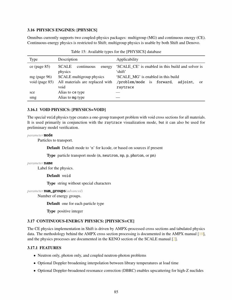
3.16 PHYSICS ENGINES: [PHYSICS]
Omnibus currently supports two coupled-physics packages: multigroup (MG) and continuous energy (CE).Continuous-energy physics is restricted to Shift; multigroup physics is usable by both Shift and Denovo.
Table 15: Available types for the [PHYSICS] database
Type Description Applicability
ce (page 85) SCALE continuous energyphysics
‘SCALE_CE’ is enabled in this build and solver is‘shift’
mg (page 96) SCALE multigroup physics ‘SCALE_MG’ is enabled in this buildvoid (page 85) All materials are replaced with
void/problem/mode is forward, adjoint, orraytrace
sce Alias to ce type —smg Alias to mg type —
3.16.1 VOID PHYSICS: [PHYSICS=VOID]
The special void physics type creates a one-group transport problem with void cross sections for all materials.It is used primarily in conjunction with the raytrace visualization mode, but it can also be used forpreliminary model verification.
parameter modeParticles to transport.
Default Default mode to ‘n’ for kcode, or based on sources if present
Type particle transport mode (n, neutron, np, p, photon, or pn)
parameter nameLabel for the physics.
Default void
Type string without special characters
parameter num_groups(advanced)Number of energy groups.
Default one for each particle type
Type positive integer
3.17 CONTINUOUS-ENERGY PHYSICS: [PHYSICS=CE]
The CE physics implementation in Shift is driven by AMPX-processed cross sections and tabulated physicsdata. The methodology behind the AMPX cross section processing is documented in the AMPX manual [10],and the physics processes are documented in the KENO section of the SCALE manual [2].
3.17.1 FEATURES
• Neutron only, photon only, and coupled neutron-photon problems
• Optional Doppler broadening interpolation between library temperatures at load time
• Optional Doppler-broadened resonance correction (DBRC) enables upscattering for high-Z nuclides
85

3.17.2 LIMITATIONS
• Photon cross sections do not include Bremsstrahlung reactions, so low-energy photon physics will notperform as expected.
• Data inconsistencies in ENDF are propagated through AMPX and may result in errors or warningsduring transport.
• Photonuclear reactions are not supported.
command ampx_kermaLoad KERMA factors from an AMPX library.
Creates splice
parameter balance_tol(advanced)Tolerance for printing a diagnostic about xs balance errors.
Default 0.005
Type real number inside (0, 1)
database [BROADEN]Temperature-corrected cross section Doppler broadening. See [PHYSICS][BROADEN] (page 93).
Optional
Applicable when
• mode is n or np; and
• not using the pole method
command ce_libSet the CE library path using SCALE file resolution.
The FileNameAliases.txt file installed to the prefix directory (usually the same as $SCALE) is usedto resolve the data location. The possible values as of SCALE 6.2.3 follow.
Table 16: SCALE CE library path aliases in SCALE 6.2.
Path Description
ce ENDF/B-VII.1ce_v7 ENDF/B-VII.0ce_v7.0 ENDF/B-VII.0ce_v7.1 ENDF/B-VII.1ce_v7_endf ENDF/B-VII.0ce_v7.0_endf ENDF/B-VII.0ce_v7.1_endf ENDF/B-VII.1
If the Omnibus build in use has the CMake variable SCALE_HPC_DATA_DIR defined, Shift will prefer-entially load HDF5 data from that instead of the XML files.
Creates ce_lib_path
parameter ce_lib_pathPath to SCALE CE Library XML or HDF5 file.
86

Type file path for reading (extension ‘.xml’ or ‘.h5’)
postprocessorThe SCALE CELibrary package must be enabled to use legacy XML CE data files.
Applicability CE library is the xml legacy format
parameter ce_pole_lib_pathPath to the HDF5 file containing pole and residue data.
Optional
Type file path for reading (extension ‘.h5’)
Applicable when
• mode is n or np; and
• CE library is in HDF5 format
parameter dbrcEnable Doppler broadened rejection correction.
DBRC adjusts the free-gas sampling of elastic scattering. In particular, it adjusts the sampling of thetarget nuclide speed when the target is a heavy nuclide.
This correction improves the accuracy of epithermal neutron scatter off of heavy nuclides. However,because it increases the rejection fraction when sampling the elastic scattering kernel, it may incur aperformance penalty.
Default True
Type boolean
Applicable when mode is n or np
parameter dbrc_energy_maxMaximum incident neutron energy for DBRC.
Default 210.0
Units eV
Type positive real number
Applicable when dbrc is True
postprocessorParameter dbrc_energy_min must be less than dbrc_energy_max.
Applicability dbrc is True
parameter dbrc_energy_minMinimum incident neutron energy for DBRC.
Default 0.4
Units eV
Type positive real number
Applicable when dbrc is True
87

parameter dbrc_lib_pathAbsolute path to the DBRC data directory.
This option can be used to override the default path to the SCALE CE DBRC data. It can only be usedwith the legacy (xml) format cross sections; HDF5 cross section libraries include the DBRC data as anew temperature-independent reaction type.
Table 17: Default DBRC data paths in SCALE 6.2.
XML CE library path DBRC library path
$DATA/ce_v7.0_endf.xml $DATA/cekenolib_7.0/dbrc/$DATA/ce_v7.1_endf.xml $DATA/cekenolib_7.1/dbrc/
Default $DATA/cekenolib_7.X/dbrc/
Type directory path for reading
Applicable when
• CE library is the xml legacy format; and
• dbrc is True
parameter disable_collision_yieldsDisables banking photons from all neutron collision reactions, but not from fission.
Default False
Type boolean
Applicable when mode is np
command energy_limitsExpand into parameters n_energy_min and n_energy_max.
Creates n_energy_min
Creates n_energy_max
database [FISSION]Fission-kinetics parameters. See [PHYSICS][FISSION] (page 94).
Default (empty database)
Applicable when neutrons are being transported
parameter kappa_libraryRead neutron fission and capture heating from the provided libary.
Optional
Type file path for reading (extension ‘.h5’)
Applicable when mode is n or np
parameter mixture_ordering(advanced)Internal sorting criterion for nuclides in the mix table.
88

Default legacy
Type legacy, ascending_density, descending_density, ascending_zaid, ordescending_zaid
parameter modeParticles to transport.
Default Default mode to ‘n’ for kcode, or based on sources if present
Type particle transport mode (n, neutron, np, p, photon, or pn)
postprocessorKcode problems must be run in mode ‘n’ or ‘np.’
parameter n_energy_maxparameter nemax
Maximum global neutron_energy cutoff for cross sections.
Default 20000000.0
Units eV
Type positive real number
Applicable when mode is n or np
postprocessorParameter n_energy_min must be less than n_energy_max.
Applicability mode is n or np
parameter n_energy_minparameter nemin
Minimum global neutron energy cutoff for cross sections.
Default 1e-05
Units eV
Type positive real number
Applicable when mode is n or np
parameter nameLabel for the physics.
Default ce
Type string without special characters
parameter num_xsgrid_pointsNumber of points used in the xs lookup acceleration grid.
Default 16384
Type positive integer
Applicable when xs_accel is True
89
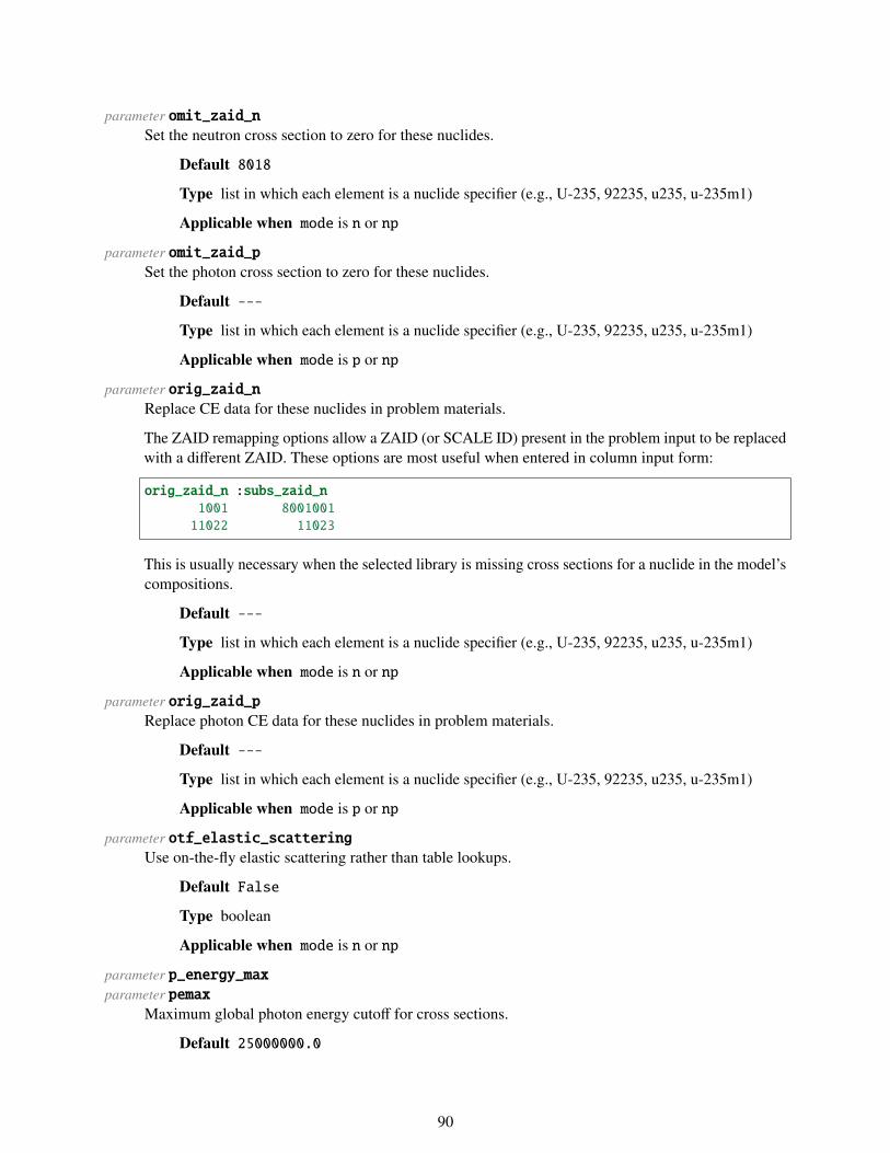
parameter omit_zaid_nSet the neutron cross section to zero for these nuclides.
Default 8018
Type list in which each element is a nuclide specifier (e.g., U-235, 92235, u235, u-235m1)
Applicable when mode is n or np
parameter omit_zaid_pSet the photon cross section to zero for these nuclides.
Default ---
Type list in which each element is a nuclide specifier (e.g., U-235, 92235, u235, u-235m1)
Applicable when mode is p or np
parameter orig_zaid_nReplace CE data for these nuclides in problem materials.
The ZAID remapping options allow a ZAID (or SCALE ID) present in the problem input to be replacedwith a different ZAID. These options are most useful when entered in column input form:
orig_zaid_n :subs_zaid_n1001 800100111022 11023
This is usually necessary when the selected library is missing cross sections for a nuclide in the model’scompositions.
Default ---
Type list in which each element is a nuclide specifier (e.g., U-235, 92235, u235, u-235m1)
Applicable when mode is n or np
parameter orig_zaid_pReplace photon CE data for these nuclides in problem materials.
Default ---
Type list in which each element is a nuclide specifier (e.g., U-235, 92235, u235, u-235m1)
Applicable when mode is p or np
parameter otf_elastic_scatteringUse on-the-fly elastic scattering rather than table lookups.
Default False
Type boolean
Applicable when mode is n or np
parameter p_energy_maxparameter pemax
Maximum global photon energy cutoff for cross sections.
Default 25000000.0
90

Units eV
Type positive real number
Applicable when mode is p or np
postprocessorParameter p_energy_min must be less than p_energy_max.
Applicability mode is p or np
parameter p_energy_minparameter pemin
Minimum global photon energy cutoff for cross sections.
Default 10000.0
Units eV
Type positive real number
Applicable when mode is p or np
parameter probability_tablesparameter ptab
Use the probability table method for the unresolved resonance region (URR).
Default True
Type boolean
Applicable when mode is n or np
parameter reactions(advanced)Reactions to load (AMPX_MT values).
Default ---
Type list in which each element is a MT number or name (e.g., N_GAMMA, 102)
sublist [SPLICE]Inject cross sections from a source other than the library. See [PHYSICS][SPLICE] (page 93).
Default (empty sublist)
parameter subs_zaid_nSubstitute ZAID corresponding to ‘orig_zaid_n.’
Default ---
Type list in which each element is a nuclide specifier (e.g., U-235, 92235, u235, u-235m1)
Applicable when mode is n or np
postprocessorThe parameters orig_zaid_n and subs_zaid_n must have the same length.
Applicability mode is n or np
parameter subs_zaid_pSubstitute ZAID corresponding to ‘orig_zaid_p.’
91

Default ---
Type list in which each element is a nuclide specifier (e.g., U-235, 92235, u235, u-235m1)
Applicable when mode is p or np
postprocessorThe parameters orig_zaid_p and subs_zaid_p must have the same length.
Applicability mode is p or np
parameter thermal_energy_cutoffThermalization energy cutoff for scattering kernels.
Default 10.0
Units eV
Type positive real number
Applicable when mode is n or np
parameter xs_accelAccelerate cross section calculation.
Accelerate total and fission cross section lookup in a material using a log-spaced energy grid. Forimproved performance, this should always be enabled when neutron transport is enabled.
Default True when neutron transport is enabled
Type boolean
Applicable when xs_cache is tot or totfisnu
parameter xs_cachePreserve cross sections between collisions.
This option enables microscopic cross sections to be cached as a particle streams between materials.This is primarily a performance optimization (in many problems it should have no effect on the results),but it subtly changes the physics of streaming through multiple materials when a neutron is in theunresolved resonance regions of the energy spectrum.
In some codes, streaming from one material to another resets the probability band values. As aconsequence, if a particle streams through two instances of the same material by traveling through avoid, its probability table band will be resampled in the second material.
Unless the xs_cache value is set to none, the physics constructs a hash table of nuclide IDs withprobability table data (and in which the particle’s energy is inside the URR) encountered since thelast collision. When streaming through the same nuclide at different temperatures, the cross sectionband [CDF] is preserved, but the cross sections will be updated for the correct temperature. This ismore physical than resetting the band at material boundaries and can affect, for example, keff of highlyvoided BWRs.
When xs_cache is set to tot, the total cross sections of all encountered nuclides will be cached. Whenthe option is set to totfisnu, the total, fission, and nu values are all pre-calculated (when a particleenters a nuclide) and cached.
Default totfisnu when problem mode is kcode else tot
Type none, ptab, tot, or totfisnu
postprocessorCannot set xs_cache to ptab unless probability_tables is True.
92

3.17.3 [PHYSICS][BROADEN]
Temperature-corrected cross section Doppler broadening.
parameter delta_tFinite difference grid spacing for Leal-Hwang temperature interpolation.
Default 1.0
Units K
Type positive real number
Applicable when not using legacy broadener
parameter energy_tolRelative difference for considering two energy points equal.
Default 1e-10
Type real number inside (0, 1)
Applicable when not using legacy broadener
parameter kinematicsInterpolate collision data.
Default False
Type boolean
parameter legacyUse legacy CE Resource interpolation.
Default False
Type boolean
Applicable when CE library is the xml legacy format
parameter temperature_tolTolerance for reusing existing broadened cross sections.
Default 4.0
Units K
Type positive real number
parameter union_energyUnionize lower and upper library temperature energy grids.
Default True
Type boolean
Applicable when not using legacy broadener
3.17.4 [PHYSICS][SPLICE]
Table 18: Available types for the [SPLICE] database
Type Description Applicability
ampx (page 94) Splice multigroup data from an AMPX library
93

3.17.5 [PHYSICS][FISSION]
Fission-kinetics parameters.
command fission_cellsGenerate ‘union_fission_cells’ and ‘union_fission_lengths’ from colon-separated unions.
Creates union_fission_cells
Creates union_fission_lengths
parameter fission_gammasparameter fiss_gam
Generate fission gammas.
Default True if and only if mode is np
Type boolean
Applicable when neutrons and photons are being transported
postprocessorcheck fission particle production options.
parameter fission_neutronsparameter fiss_neut
Generate fission neutrons.
Default True if and only if mode is not kcode
Type boolean
parameter union_fission_cells(advanced)Flattened list of cells in each union.
Default (empty sublist)
Type list of cell names (each element is a string)
parameter union_fission_lengths(advanced)Number of cells per union in the above list.
Default (empty sublist)
Type list in which each element is a integer
3.17.6 [PHYSICS][SPLICE=AMPX]
The AMPX data splicing option allows multigroup data from an AMPX library to be spliced into the CEtransport. This feature allows specialized reactions to be calculated during transport (e.g., KERMA tallies).
Currently, only multigroup reaction rates can be inserted. No probability tables or collision data can beinserted.
If a CE reaction is already present, the AMPX splicer will not override it. To get around this, the user canmanually specify the list of reactions to load in the Continuous-energy physics: [PHYSICS=ce] (page 85)block, omitting the reactions to be loaded as multigroup data.
command mg_libSet mg_lib to the given value using SCALE DATA resolution.
94
Creates xs_library
parameter nameDescriptive name for the data being spliced in.
Type string without special characters
parameter orig_zaid_nReplace MG data for these nuclides in problem materials.
Default ---
Type list in which each element is a nuclide specifier (e.g., U-235, 92235, u235, u-235m1)
parameter orig_zaid_pReplace photon MG data for these nuclides in problem materials.
Default ---
Type list in which each element is a nuclide specifier (e.g., U-235, 92235, u235, u-235m1)
parameter reactions(advanced)Multigroup reactions to splice into the CE data (AMPX_MT values).
Default (empty sublist)
Type list in which each element is a MT number or name (e.g., N_GAMMA, 102)
parameter subs_zaid_nSubstitute ZAID corresponding to ‘orig_zaid_n.’
Default ---
Type list in which each element is a nuclide specifier (e.g., U-235, 92235, u235, u-235m1)
postprocessorThe parameters orig_zaid_n and subs_zaid_n must have the same length.
parameter subs_zaid_pSubstitute ZAID corresponding to ‘orig_zaid_p.’
Default ---
Type list in which each element is a nuclide specifier (e.g., U-235, 92235, u235, u-235m1)
postprocessorThe parameters orig_zaid_p and subs_zaid_p must have the same length.
parameter xs_libraryPath to AMPX library to load data.
Type file path for reading
95

3.18 MULTIGROUP PHYSICS: [PHYSICS=MG]
The SCALE multigroup physics package as implemented in Exnihilo can use various multigroup cross sectionlibrary formats, including:
• AMPX-processed cross sections [10],
• User-defined macroscopic cross sections,
• GIP format macroscopic cross sections, and
• ANISN-formatted multigroup libraries [19].
When compositions (as opposed to user-specified multigroup cross sections) are provided, Omnibus usesSCALE to calculate infinite homogeneous medium cross sections for all materials. No self-shielding isperformed. The default cross section processing is primarily intended for generating deterministic solutionsfor hybrid calculations.
Warning: The default multigroup cross sections generated by Omnibus are only recommended forqualitative transport behavior. Obtaining accurate multigroup cross sections for general problems requiresa great deal of experience using SCALE cross section processing that incorporates self-shielding.
The Monte Carlo implementation of MG physics uses the same methods as KENO multigroup physics.Depending on the scattering order of the overall problem and of each particular material, the scattering modeltakes three forms.
• Isotropic scattering has the standard physical formulation.
• P1 scattering forces the particle to scatter with an exiting cosine equal to the mean cosine. That is,instead of sampling the exiting cosine from a linear distribution, the cosine is sampled from a deltafunction equal to µ0 =
∫ 1−1 µσs(µ) dµ. Thus, in an isotropically scattering medium in a P1 problem,
the particle’s exiting direction will be exactly perpendicular to the particle’s incident direction (sinceisotropic scattering has µ0 = 0). This is not physical, but it is the physics behavior in MG KENO.
• Higher order PN scattering selects exiting angles from a quadrature.
3.18.1 FEATURES
• Neutron only, photon only, and coupled neutron-photon problems
3.18.2 LIMITATIONS
• Anisotropic Monte Carlo particle scattering uses the same angular approximations as the multigroupKENO package in SCALE.
parameter ampx_pathPath to an AMPX working library input file.
This input requires a working library with at least the number of materials present in the model. For alibrary with N materials, the cross sections for matids (page 43) [0,N) are assigned based on the ids ofmaterials in the AMPX file after being sorted in ascending order. For example, if a working library hasmaterials with IDs [1, 21, 12] (intentionally unsorted); the mapping of material IDs to AMPX libraryIDs is
96

0 -> 11 -> 122 -> 21
There is an additional option implicit_void (page 99) that assigns void cross sections to matid 0. Thusif the AMPX library has media IDs 1, 3, 5, and if implicit_void is true, then the mapping will be
0 -> 01 -> 12 -> 33 -> 5
Type file path for reading (extension ‘.ampx’)
Applicable when xsgen is ampx
parameter anisn_info_pathPath to an ADVANTG-format ANISN metadata file.
Type file path for reading (extension ‘.info’)
Applicable when xsgen is anisncomp
command anisn_libSet ANISN library and metadata paths using a search path.
Creates anisn_path
Creates anisn_zaid_path
Creates anisn_info_path
parameter anisn_pathPath to an ANISN cross section input.
Type file path for reading (extension ‘.bin’)
Applicable when xsgen is anisncomp
parameter anisn_tableANISN table IDs corresponding to anisn_zaid.
Default ---
Type list in which each element is a positive integer
Applicable when xsgen is anisncomp
postprocessorThe parameters anisn_zaid and anisn_table must have the same length.
Applicability xsgen is anisncomp
parameter anisn_zaidReplace the given ZAIDs with corresponding ANISN table IDs.
Default ---
97

Type list in which each element is a nuclide specifier (e.g., U-235, 92235, u235, u-235m1)
Applicable when xsgen is anisncomp
parameter anisn_zaid_pathPath to an ADVANTG-format ANISN zaid map.
Type file path for reading (extension ‘.zaid’)
Applicable when xsgen is anisncomp
parameter disable_upscatteringparameter noup
Remove upscattering by altering cross sections.
For shielding calculations, thermal neutrons may contribute little to the detector response. However,converging the distribution of thermal neutrons through upscatter iterations can be expensive.
This option adjusts all material cross sections so that their scattering matrix is strictly lower triangular.The default behavior is to lump upscattering cross sections into within-group scattering, adjusting theoutscatter cross sections so that:
σs,g,g ←
g∑g′=1
σs,g,g′
σs,g,g′ ← 0, g′ = [1, . . . , g − 1]
where the outscatter cross section is
σs(Eg → Eg′) ≡ σs,g,g′
Default True if only transporting photons or using hybrid solve
Type boolean
command energy_limitsExpand into parameters n_energy_min and n_energy_max.
Creates n_energy_min
Creates n_energy_max
database [GIP]GIP input file metadata. See [PHYSICS][GIP] (page 104).
Applicable when xsgen is gip
parameter gip_pathPath to a GIP working library file.
Type file path for reading (extension ‘.gip’)
Applicable when xsgen is gip
parameter implicit_captureEnable implicit capture for Monte Carlo transport.
Default True
98

Type boolean
Applicable when solver is ‘shift’
parameter implicit_void(advanced)Insert ‘void’ material of matid=0 before AMPX-specified mats.
Default False
Type boolean
Applicable when xsgen is ampx
parameter mc_pn_scattering(advanced)Enable high-order scattering for MC transport.
Default True when Shift is enabled
Type boolean
Applicable when PN order is greater than 1
postprocessorMultigroup Monte Carlo transport requires pn_order to be zero or odd.
Applicability mc_pn_scattering is True
command mg_libSet mg_lib to the given value using SCALE DATA resolution.
The aliases for the SCALE multigroup libraries can be found at INSTALL/etc/LibraryAliases.txt. The SCALE FileNameAliases.txt file is used to resolve the data files. The current optionsfor multigroup libraries are:
Table 19: Multigroup physics library aliases and filenames in SCALE 6.2.
99

Alias for mg_lib Filename
broad_n xn56v7.1broad_ng xn28g19v7.1fine_n xn252v7.1fine_ng xn200g47v7.1ultra_fine_n xn999v7.1v7-238 xn238v7.0v7-238n xn238v7.0v7.0-238n xn238v7.0xn238v7 xn238v7.0v7-252n xn252v7.1v7.1-252 xn252v7.1v7.1-252n xn252v7.1v7-200n47g xn200g47v7.1v7.1-200n47g xn200g47v7.1v7.0-200n47g xn200g47v7.0v7-27n19g xn27g19v7.0v7.0-27n19g xn27g19v7.0v7-28n19g xn28g19v7.1v7.1-28n19g xn28g19v7.1v7-56 xn56v7.1v7-56n xn56v7.1v7.1-56 xn56v7.1v7.1-56n xn56v7.1v7-999 xn999v7.0v7-999n xn999v7.0v7.1-999 xn999v7.1v7.1-999n xn999v7.1test_n test8g_v7.1test-8grp test8g_v7.1
Creates xs_library
parameter modeParticles to transport.
Default Default mode to ‘n’ for kcode, or based on sources if present
Type particle transport mode (n, neutron, np, p, photon, or pn)
postprocessorKcode problems must be run in mode ‘n’ or ‘np.’
parameter n_energy_maxparameter nemax
Maximum global neutron_energy cutoff for cross sections.
Default 20000000.0
Units eV
100

Type positive real number
Applicable when mode is n or np
postprocessorParameter n_energy_min must be less than n_energy_max.
Applicability mode is n or np
parameter n_energy_minparameter nemin
Minimum global neutron energy cutoff for cross sections.
Default 1e-05
Units eV
Type positive real number
Applicable when mode is n or np
parameter nameLabel for the physics.
Default mg
Type string without special characters
parameter neutron_boundsparameter nbounds
Neutron group boundaries.
Default ---
Type positive floats in decreasing order (each element is a positive real number)
Applicable when xsgen is ampx, gip, inline, or xml
parameter num_groups(advanced)Number of energy groups.
Default based on given user input
Type positive integer
postprocessorInline and GIP cross section definitions require group boundaries.
Applicability xsgen is gip or inline
parameter omit_zaidOmit the provided nuclides from the XS processing.
Default ---
Type list in which each element is a nuclide specifier (e.g., U-235, 92235, u235, u-235m1)
Applicable when xsgen is scalecomp or anisncomp
parameter orig_zaidReplace MG data for these nuclides in problem materials.
101

Default ---
Type list in which each element is a nuclide specifier (e.g., U-235, 92235, u235, u-235m1)
Applicable when xsgen is scalecomp or anisncomp
parameter p_energy_maxparameter pemax
Maximum global photon energy cutoff for cross sections.
Default 25000000.0
Units eV
Type positive real number
Applicable when mode is p or np
postprocessorParameter p_energy_min must be less than p_energy_max.
Applicability mode is p or np
parameter p_energy_minparameter pemin
Minimum global photon energy cutoff for cross sections.
Default 10000.0
Units eV
Type positive real number
Applicable when mode is p or np
parameter photon_boundsparameter pbounds
Photon group boundaries.
Default ---
Type positive floats in decreasing order (each element is a positive real number)
Applicable when xsgen is ampx, gip, inline, or xml
parameter pn_orderScattering order of problem.
Type non-negative integer
parameter processingType of cross section processing to apply.
Default fulcrum
Type fulcrum or none
Applicable when xsgen is scalecomp
parameter subs_zaidSubstitute ZAID corresponding to ‘orig_zaid.’
102

Default ---
Type list in which each element is a nuclide specifier (e.g., U-235, 92235, u235, u-235m1)
Applicable when xsgen is scalecomp or anisncomp
postprocessorThe parameters orig_zaid and subs_zaid must have the same length.
Applicability xsgen is scalecomp or anisncomp
parameter subtract_upscatteringparameter subup
Remove upscattering by subtracting from the total cross section.
Instead of lumping upscatter cross sections into the self-scattering cross section, delete the upscattercross sections and reduce the total cross section accordingly.
σt,g ← σt,g −
g−1∑g′=1
σs,g,g′
σs,g,g′ ← 0, g′ = [1, . . . , g − 1]
where the outscatter cross section is
σs(Eg → Eg′) ≡ σs,g,g′
Default False
Type boolean
Applicable when disable_upscattering is True
parameter transport_correctionModify the anisotropy of the scattering cross sections to help preserve solution positivity.
Default none
Type diagonal, cesaro, or none
postprocessorThe cesaro transport correction requires pn_order >= 2.
Applicability transport_correction is cesaro
parameter xml_pathPath to an XML cross section input file.
Type file path for reading (extension ‘.xml’)
Applicable when xsgen is xml
sublist [XS]Manual isotropic cross section input. See [PHYSICS][XS] (page 105).
Applicable when xsgen is inline
parameter xs_librarySCALE multigroup library name or master library path.
103

Type file path for reading
Applicable when xsgen is scalecomp
parameter xsgen(advanced)Type of cross section data input.
The xsgen parameter specifies in what format the cross sections are defined for multigroup physics. Itis defined automatically by the front end (based on what input the user provides) and should not everhave to be set manually.
Table 20: Possible cross section input formats.
Option Description
inline The [XS] (page 105) subdatabase is used to define crosssections for every material.
ampx The cross sections for every material are defined in AMPXformat. This file is specified using the ampx_path parame-ter.
gip The cross sections for every material are defined in GIPformat. This file is specified using the gip_path parameter.Other required parameters describing the file must be in the[GIP] sub-database.
scalecomp SCALE multigroup cross sections will be built from compo-sition information pulled from the model.
anisncomp Mixed cross sections will be calculated fromANISN/ADVANTG multigroup libraries using com-positions pulled from the model.
xml The cross sections for every material are defined in a separateXML file format. This file is specified using the xml_pathparameter.
Default based on the user-given input types
Type scalecomp, anisncomp, ampx, gip, inline, or xml
3.18.3 [PHYSICS][GIP]
The GIP file format is supported only for legacy applications. It is essentially a Fortran data dump. Eachgroup of data is written as a single Fortran record comprised of a (num_reactions, num_moments,num_materials) array. The number of reactions here is equal to ihm plus an extra value if upscattering ispresent.
parameter ihmCross section table length in GIP file.
Type non-negative integer
parameter ihsPosition of within-group scattering in GIP file.
Type non-negative integer
104

parameter ihtPostition of total cross section in GIP file.
Type non-negative integer
parameter isctPN scattering order in GIP file.
Type non-negative integer
parameter iupsNumber of thermal (upscatter) groups in GIP file.
Type non-negative integer
parameter nmatNumber of materials in GIP file.
Type non-negative integer
parameter strictWhether edit cross sections correspond to the GIP standard.
With the strict option, the “edit” reactions on the GIP file are assumed to have the followinginterpretation:
Table 21: GIP reaction tables.
Table Reaction
iht - 4 χ
iht - 3 Σfiht - 2 Σaiht - 1 νΣf
Default False
Type boolean
3.18.4 [PHYSICS][XS]
This sub-database specifies all cross sections for a single material. If the material is fissionable, all offission, nu, and chi must be present. If it is not fissionable, then none of them can be present.
parameter chiFission spectrum.
Default ---
Type list of non-negative floats (each element is a non-negative real number)
postprocessorThe parameters total, fission, nu, and chi must have the same length. Empty lists are ignored.
parameter fissionFission cross section.
Default ---
105

Type list of non-negative floats (each element is a non-negative real number)
parameter matidMaterial ID.
Type non-negative integer
parameter nameLabel for the material.
Default given matid
Type string without special characters
parameter nuNeutron production.
Default ---
Type list of non-negative floats (each element is a non-negative real number)
parameter s0Isotropic scattering cross section.
Type list of non-negative floats (each element is a non-negative real number)
parameter totalTotal cross section by group.
Type list of non-negative floats (each element is a non-negative real number)
3.19 COMPOSITIONS: [COMP]
The [COMP] block controls output and management of compositions and enables defining them manually.The matids in each block must correspond to the matids in the problem geometry.
command autocolorAttempt to provide color values using their compositions.
Creates color_key
Creates color_val
Applicable when
• ‘ENABLE_PYTHON_WRAPPERS’ is enabled in this CMake build; and
• The ‘matplotlib’ python package is installed
parameter color_key(advanced)Name of compositions for which colors are being set.
Default ---
Type list in which each element is a string
parameter color_val(advanced)Compositions color to be set.
Default ---
106

Type list in which each element is a X11 color, HTML color like #FF00ee, tuple, or empty
postprocessorThe parameters color_key and color_val must have the same length.
command colorsMap ‘color_key’ to ‘color_val’ from pairs or arrow-separated items.
VisIT supports custom colors to be associated with each material in its plotting routines. Materials notspecified in this list will be filled with grey. Incorrect material names will generate an error:
colorsm1 "light blue""void" "dark grey"m13 "#aaeeff"m14 "DarkSlateGray"m105 "#5555FF"m106 "pale goldenrod"
Valid color names are either HTML-style hexadecimal RGB tuples or X11 colors.
For complicated inputs with variable materials, the Python raytracer and coloring modules can beused to automatically assign colors based on materials compositions. (See the omnibus.raytracer.colors module.)
Creates color_key
Creates color_val
parameter compgen(advanced)Type of composition input.
Default based on the user-given comp types
Type model, hdf5, or inline
sublist [COMPOUND]Elemental compound definition. See [COMP][COMPOUND] (page 110).
Default (empty sublist)
command elementsCreate compounds from natural abundances of the given elements.
Creates compound
deprecated force_sclDeprecated entry force_scl has been renamed to load_scl.
Update to load_scl
parameter inputPath to the HDF5 file containing compositions.
Type file path for reading (extension ‘.h5’)
Applicable when compgen is hdf5
107

parameter load_sclLoad nuclides from the SCALE Standard Composition Library.
The SCALE standard composition library (SCL) provides a database of nuclides, elements, andcompounds that can be used to simplify user composition input.
Exnihilo uses a global database of nuclide data (number densities, names, atomic numbers, etc.) forconstruction of compositions. This same database is also used to drive SCALE’s multigroup crosssection builder Fulcrum. If using the SCALE cross section builder (xsgen processed), the names inthe database must correspond to the names SCALE expects.
Some model types (Geant4, Lava) are able to load nuclide metadata independently of the SCALE SCL;this can interfere with cross section generation. The load_scl option preferentially loads SCALE’snuclide definitions.
This option is also useful if using a composition source (hdf5 or inline) that has incomplete nuclidedata but is being used for depletion. For example, since only nuclides in use by the current compositionset are written to the composition output, it may not be sufficient to use those compositions/nuclides ina depletion run (since additional depletion nuclides will be added to the composition and their nuclidedata may be missing).
Note that changing the nuclide data source will change the relationship between composition numberdensities and weight fractions, so output values may change.
Default True when using ‘processed’ MG physics, CE physics, or HDF5/inline materials
Type boolean
Applicable when ‘SCALE_StdCompLib’ is enabled in this build
sublist [MATERIAL]Composition definition. See [COMP][MATERIAL] (page 109).
Applicable when compgen is inline
database [NUCLIDES]Nuclide definitions. See [COMP][NUCLIDES] (page 110).
Optional
parameter outputSave compositions to the output file.
Default True
Type boolean
parameter sclib_pathPath to the SCALE standard composition library.
Default '/.../scale.rev40.sclib'
Type file path for reading (extension ‘.sclib’)
Applicable when load_scl is True
108
3.19.1 [COMP][MATERIAL]
The material block is for defining an individual composition. Providing any materials will override allcompositions that may be present in the model (page 43).
parameter depleteparameter depl
Flag the material as depletable.
Marking a material as “depletable” tells Shift to enable ORIGEN depletion for this material unless theuser overrides this using the options in the [DEPLETION] database.
The default value of “auto” will set this property to true if and only if it is marked as fissionable.
Default auto
Type auto, true, or false
parameter fissionparameter fiss
Flag the material as fissionable.
Marking a material as “fissionable” sets whether (by default) fission gammas and neutrons will beproduced during fixed-source transport. In other words, setting this value to false will (again, bydefault) suppress secondary neutrons or gamma yields from the material.
Note that this option is ignored for fission site sampling in kcode/eigenvalue mode: all fissionablenuclides have a chance to create fission sites.
The default value of “auto” will set this property to true if any fissionable nuclide is present, and falseif not.
Default auto
Type auto, true, or false
parameter matidInternal matid number.
The matid is a [0,N)-indexed internal numbering system. The matids used by Shift typically differfrom the material names used in the problem physics input (for example, m10 in an MCNP inputdeck might correspond to matid=1). Currently, the only way to guarantee that this corresponds to aparticular material in the geometry input is to use an input that specifies matids explicitly (RTK ormesh geometry). However, by viewing the matid-to-label mapping given in an Omnibus post-processoutput for a SCALE or MCNP input geometry, it is possible to determine what matid corresponds towhat material in a particular problem input.
Type non-negative integer
parameter nameLabel for the material.
Type non-empty string
parameter ndNumber densities of each nuclide.
Units atom(b·cm)
109

Type list in which each element is a positive real number
postprocessorThe parameters nd and zaid must have the same length.
parameter temperatureparameter tmp
Material temperature.
Units K
Type non-negative real number
parameter zaidElement/nuclide IDs (MZZZAAA) in this material.
Type list in which each element is a positive integer
3.19.2 [COMP][NUCLIDES]
Define properties for a given nuclide ID. This enables custom ZAID values in input files such as multigroupcross section data. These properties will override any existing masses loaded from the SCALE SCL.
parameter massAtomic masses of nuclides.
Type list in which each element is a positive real number
postprocessorThe parameters name, zaid, and mass must have the same length.
parameter nameNames of nuclides.
Type list in which each element is a string
parameter zaidNuclide IDs (MZZZAAA).
Type list in which each element is a positive integer
3.19.3 [COMP][COMPOUND]
Define compounds or natural-abundance elements. Any ZAID in the user model or composition definitionscorresponding to the value of czaid will be expanded into the zaid values provided for this compound.These will override any compound defined by the SCALE SCL.
parameter czaidCompound ZAID (e.g., 1000 for elemental hydrogen).
Type positive integer
parameter nameDescriptive name of the compound.
Type string without special characters
parameter wtfracWeight fraction of each constituent.
110

Type list in which each element is a positive real number
postprocessorThe parameters wtfrac and zaid must have the same length.
parameter zaidConsitutent nuclide IDs (MZZZAAA).
Type list in which each element is a positive integer
3.20 RESPONSES: [RESPONSE]The RESPONSE block is for defining energy- and particle-dependent responses such as dose conversionfactors. Each response can be used multiple times in the tallies.
Table 22: Available types for the [RESPONSE] database
Type Description Applicability
histogram (page 111) Histogram responseinterpolated (page 112) Interpolation between valuesxs (page 112) Microscopic cross section multiplier
3.20.1 [RESPONSE=HISTOGRAM]The “histogram” response is effectively a piecewise constant cross section. The response is the specifiedvalue of the response (page 111) parameter inside the corresponding energy (page 111) bin for the givenparticle type (page 111). The response is zero for other particle types or outside the given energy range.
parameter descriptionOptional longer descriptive string.
Default ''Type string
parameter energyparameter e
Lowest bound plus upper bounds for the histograms.
Units eV
Type monotonically increasing list (each element is a real number)
parameter nameShort title or label for response.
Type string without special characters
parameter particle_typeparameter pt
Particle type to apply this response.
Type particle type (n, neutron, p, or photon)
parameter responseparameter r
Histogram response values.
Type list in which each element is a real number
postprocessorSize of energy bounds must be one greater than the number of response values.
111

3.20.2 [RESPONSE=INTERPOLATED]
Interpolation between values.
parameter descriptionOptional longer descriptive string.
Default ''
Type string
parameter energyparameter e
Energy points.
Units eV
Type monotonically increasing list (each element is a positive real number)
parameter interpolation_typeparameter interp
Type of interpolated response.
Type linear, log_lin, lin_log, or log_log
parameter nameShort title or label for response.
Type string without special characters
parameter particle_typeparameter pt
Particle type to apply this response.
Type particle type (n, neutron, p, or photon)
parameter responseparameter r
Response values at energy points.
Type list in which each element is a real number
postprocessorResponse must be positive for log_log or log_lin.
postprocessorThe parameters energy and response must have the same length.
3.20.3 [RESPONSE=XS]
Microscopic cross section multiplier.
parameter densityDensity multiplier for response calculation.
Default 1.0
Type positive real number
112

parameter descriptionOptional longer descriptive string.
Default ''
Type string
parameter mtReaction to tally.
Type MT number or name (e.g., N_GAMMA, 102)
parameter nameShort title or label for response.
Type string without special characters
parameter nuclideNuclide ID for the cross section.
Type nuclide specifier (e.g., U-235, 92235, u235, u-235m1)
parameter particle_typeparameter pt
Particle type to apply this response.
Type particle type (n, neutron, p, or photon)
parameter physics(advanced)Name of the physics DB to use for the source data.
Default the name of the CE physics database
Type string without special characters
parameter temperatureparameter tmp
Temperature of nuclide.
Type positive real number
Applicable when particle_type is n
3.21 TALLIES: [TALLY]
Be aware that unless otherwise specified, tallies in Shift:
• are replicated, even if domain decomposition is requested;
• use history-based statistics to estimate variance;
• provide volume-averaged reaction rates if the tally region’s volume is known;
• are path length estimators.
113

Many tallies support a common set of attributes, including a name and optional description, a list of reactionsto tally, a list of [RESPONSE] (page 111) objects, and neutron and photon energy bin boundaries.
Note: Unlike other Monte Carlo transport codes, the bin boundaries in Omnibus are truly boundaries, notupper or lower energies. Therefore, the number of energy bins will be one less than the number of bounds.To reproduce the behavior of MCNP and Monaco, which tally from the cutoff energy to the lowest givenenergy, the user must explicitly add the cutoff energy as the lowest energy bound.
The cell and mesh tallies produce volume averaged quantities when volumes are available for the regionbeing tallied. Therefore, a reaction rate is output as a reaction rate density (units of reaction
s−cm3 ). If volumes arenot provided (explicitly by the user or automatically by the geometry) for cell tallies, a warning will be issuedand the tally result will be cell-integrated.
Warning: Many geometries define the volume of a cell to be the volume for an instance of that cell.If the cell is replicated (e.g., a pin cell in an assembly), then the volume being used to normalize thetally might not correspond to the total volume being tallied. This is because all instances of a cell willcontribute to the same tally.
Because of the potential ambiguities that may occur with volume normalization, it is highly recommendedthat users check the volumes field output alongside cell tallies. A volume entry of 0 means that the volumewas not provided, so that the corresponding tally will have units of reaction
s as though the tally region had unitvolume.
sublist [BATCH_MESH](advanced)Tally reaction rates using batch statistics (experimental!). See [TALLY][BATCH_MESH] (page 160).
Applicable when problem mode is kcode
Optional
sublist [BIRTH_SPECTRUM]Tally the energy distribution of particles at birth in geometry cells. See [TALLY][BIRTH_SPECTRUM](page 158).
Optional
Applicable when solver is ‘shift’
sublist [CELL]Tally reaction rates in geometry cells and unions of cells. See [TALLY][CELL] (page 130).
Optional
sublist [CYLMESH]Tally reaction rates in cylindrical cells. See [TALLY][CYLMESH] (page 123).
Optional
sublist [DIAGNOSTIC]Singleton tallies used for transport diagnostic purposes. See [TALLY][DIAGNOSTIC] (page 140).
Applicable when solver is ‘shift’
114

Default (empty sublist)
sublist [HEXMESH]Tally reaction rates on a hexagonal grid. See [TALLY][HEXMESH] (page 127).
Optional
sublist [HEXNODAL]Tally integral quantities on a hexagonal mesh for nodal calculations. See [TALLY][HEXNODAL](page 150).
Applicable when solver is ‘shift’
Optional
sublist [MEAN_SCATTER_ANGLE]Tally the mean scattering angle in geometry cells. See [TALLY][MEAN_SCATTER_ANGLE](page 156).
Optional
Applicable when solver is ‘shift’
sublist [MESH]Tally reaction rates on a domain-decomposed Cartesian mesh. See [TALLY][MESH] (page 116).
Optional
sublist [MESH_SURFACE]Tally reaction rates and partial currents on mesh faces. See [TALLY][MESH_SURFACE] (page 121).
Optional
sublist [MICRO]Tally flux and microscopic cross sections in materials. See [TALLY][MICRO] (page 138).
Applicable when
• solver is ‘shift’; and
• physics is CE
Optional
sublist [MIGRATION_AREA]Tally particle migration area on a Cartesian mesh. See [TALLY][MIGRATION_AREA] (page 154).
Applicable when solver is ‘shift’
Optional
sublist [NODAL]Tally integral quantities on a Cartesian mesh for nodal calculations. See [TALLY][NODAL] (page 146).
Applicable when solver is ‘shift’
Optional
sublist [SCATTERING_PROB_MATRIX]Tally the group-to-group scattering probability matrix in geometry cells. See[TALLY][SCATTERING_PROB_MATRIX] (page 157).
115

Optional
Applicable when solver is ‘shift’
database [SENSITIVITY]Tally sensitivities for use in uncertainty quantification. See [TALLY][SENSITIVITY] (page 144).
Optional
Applicable when
• physics is CE; and
• ‘Sensitivity’ is enabled in this build
sublist [SHADOW]Tally arbitrary cells in an overlaid but non-interacting geometry. See [TALLY][SHADOW] (page 135).
Applicable when ‘GG’ is enabled in this build
Optional
sublist [SURFACE_CENSUS]Tally individual particle properties as they cross a geometry surface. See[TALLY][SURFACE_CENSUS] (page 159).
Applicable when solver is ‘shift’
Optional
database [SWORD]Include tally definitions from SWORD input. See [TALLY][SWORD] (page 141).
Optional
Applicable when model is ‘sword’
sublist [VERA]Tally in cells in a VERA model. See [TALLY][VERA] (page 134).
Optional
3.21.1 [TALLY][MESH]
Shift supports multiple structured Cartesian path length mesh tallies. The mesh can be defined over all or partof the physical problem geometry. If domain decomposition is enabled in Shift, only the part of the meshtally that is present on a spatial domain will be transported on.
parameter cyclesThe kcode problem phase in which this tally is active.
Default active
Type active or inactive
Applicable when problem mode is kcode
parameter delta_xLength of mesh tally cell on the X axis.
Units cm
116

Type positive real number
Applicable when type is global
parameter delta_yLength of mesh tally cell on the Y axis.
Units cm
Type positive real number
Applicable when type is global
parameter delta_zLength of mesh tally cell on the Z axis.
Units cm
Type positive real number
Applicable when type is global
command deltasExpand into parameters delta_x, delta_y, and delta_z.
Creates delta_x
Creates delta_y
Creates delta_z
parameter descriptionparameter desc
Optional longer descriptive string.
Default ''
Type string
database [FILTERS]Tally filtering options. See [TALLY][MESH][FILTERS] (page 161).
Optional
parameter macro_mtENDF reactions for partial macroscopic cross section tallying.
Default ---
Type list of MT numbers or names (each element is a MT number or name (e.g.,N_GAMMA, 102))
Applicable when physics is CE
parameter macro_mt_zaidNuclide IDs for partial macroscopic cross section tallying.
Default ---
Type list in which each element is a nuclide specifier (e.g., U-235, 92235, u235, u-235m1)
Applicable when physics is CE
117

parameter macro_rxnSpecial reactions for macroscopic cross section tallying.
Default ---
Type list in which each element is a flux, pos_partial_current_x,neg_partial_current_x, pos_partial_current_y, neg_partial_current_y,pos_partial_current_z, neg_partial_current_z, total, absorption,scattering, transfer_1n, transfer_2n, transfer_3n, transfer_4n,fission, nu_fission, kappa_sigma, kappa_sigma_f, or kappa_sigma_c
Applicable when physics is CE
parameter macro_rxn_zaidNuclide IDs for macroscopic ‘special reaction’ cross section tallying.
Default ---
Type list in which each element is a nuclide specifier (e.g., U-235, 92235, u235, u-235m1)
Applicable when physics is CE
parameter micro_mtENDF reactions for microscopic cross section tallying.
Default ---
Type list of MT numbers or names (each element is a MT number or name (e.g.,N_GAMMA, 102))
Applicable when physics is CE
postprocessorThe parameters micro_mt_zaid and micro_mt must have the same length.
Applicability physics is CE
parameter micro_mt_zaidNuclide IDs for microscopic cross section tallying.
Default ---
Type list in which each element is a nuclide specifier (e.g., U-235, 92235, u235, u-235m1)
Applicable when physics is CE
parameter micro_rxnSpecial reactions for microscopic cross section tallying.
Default ---
Type list in which each element is a flux, pos_partial_current_x,neg_partial_current_x, pos_partial_current_y, neg_partial_current_y,pos_partial_current_z, neg_partial_current_z, total, absorption,scattering, transfer_1n, transfer_2n, transfer_3n, transfer_4n,fission, nu_fission, kappa_sigma, kappa_sigma_f, or kappa_sigma_c
Applicable when physics is CE
118

postprocessorThe parameters micro_rxn_zaid and micro_rxn must have the same length.
Applicability physics is CE
parameter micro_rxn_zaidNuclide IDs for microscopic ‘special reaction’ cross section tallying.
Default ---
Type list in which each element is a nuclide specifier (e.g., U-235, 92235, u235, u-235m1)
Applicable when physics is CE
deprecated micro_zaidDeprecated entry micro_zaid has been renamed to micro_mt_zaid.
Update to micro_mt_zaid
parameter mtAdditional macroscopic reaction rates to tally.
Default ---
Type list of MT numbers or names (each element is a MT number or name (e.g.,N_GAMMA, 102))
Applicable when physics is CE
parameter nameShort title or label for the tally.
Type string without special characters
parameter neutron_binsparameter nbins
Energy bin boundaries for neutrons.
Default ---
Units eV
Type nonnegative floats in decreasing order (each element is a non-negative real number)
parameter normalizationConstant multiplicative factor to apply to tally results.
Default 1.0
Type positive real number
parameter photon_binsparameter pbins
Energy bin boundaries for photons.
Default ---
Units eV
Type nonnegative floats in decreasing order (each element is a non-negative real number)
119

parameter reactionsparameter rxn
Reactions to calculate for this tally.
Default flux
Type list in which each element is a flux, pos_partial_current_x,neg_partial_current_x, pos_partial_current_y, neg_partial_current_y,pos_partial_current_z, neg_partial_current_z, total, absorption,scattering, transfer_1n, transfer_2n, transfer_3n, transfer_4n,fission, nu_fission, kappa_sigma, kappa_sigma_f, or kappa_sigma_c
parameter responsesparameter resp
Responses for this tally.
Default ---
Type list in which each element is a string
postprocessorValidate response names against [RESPONSE] blocks.
parameter typeType of mesh tally.
Default grid
Type grid or global
parameter xTally grid coordinates along the X axis.
Units cm
Type monotonically increasing list with at least two values (each element is a real number)
Applicable when type is grid
parameter yTally grid coordinates along the Y axis.
Units cm
Type monotonically increasing list with at least two values (each element is a real number)
Applicable when type is grid
parameter zTally grid coordinates along the Z axis.
Units cm
Type monotonically increasing list with at least two values (each element is a real number)
Applicable when type is grid
120
3.21.2 [TALLY][MESH_SURFACE]
The Cartesian mesh surface tally can calculate surface flux, current, or partial current on each face of themesh. The allowed reactions for this tally differ from the volumetric mesh tally (page 116) reactions.
parameter cyclesThe kcode problem phase in which this tally is active.
Default active
Type active or inactive
Applicable when solver is ‘shift’
parameter delta_xLength of mesh current tally cell on the X axis.
Units cm
Type positive real number
Applicable when type is global
parameter delta_yLength of mesh current tally cell on the Y axis.
Units cm
Type positive real number
Applicable when type is global
parameter delta_zLength of mesh current tally cell on the Z axis.
Units cm
Type positive real number
Applicable when type is global
command deltasExpand into parameters delta_x, delta_y, and delta_z.
Creates delta_x
Creates delta_y
Creates delta_z
parameter descriptionparameter desc
Optional longer descriptive string.
Default ''
Type string
database [FILTERS]Tally filtering options. See [TALLY][MESH][FILTERS] (page 161).
Optional
121

parameter nameShort title or label for the tally.
Type string without special characters
parameter neutron_binsparameter nbins
Energy bin boundaries for neutrons.
Default ---
Units eV
Type nonnegative floats in decreasing order (each element is a non-negative real number)
parameter normalizationConstant multiplicative factor to apply to tally results.
Default 1.0
Type positive real number
parameter photon_binsparameter pbins
Energy bin boundaries for photons.
Default ---
Units eV
Type nonnegative floats in decreasing order (each element is a non-negative real number)
parameter reactionsparameter rxn
Type of mesh surface tally.
Default flux
Type list in which each element is a flux, current, partial_current_negative, orpartial_current_positive
parameter typeType of mesh surface tally.
Default grid
Type grid or global
parameter xMesh current tally coordinates along the X axis.
Units cm
Type monotonically increasing list with at least two values (each element is a real number)
Applicable when type is grid
parameter yMesh current tally coordinates along the Y axis.
Units cm
122

Type monotonically increasing list with at least two values (each element is a real number)
Applicable when type is grid
parameter zMesh current tally coordinates along the Z axis.
Units cm
Type monotonically increasing list with at least two values (each element is a real number)
Applicable when type is grid
3.21.3 [TALLY][CYLMESH]
Particles can be tracked on a translated, rotated cylinder broken into (r, z, θ) mesh cells.
parameter cyclesThe kcode problem phase in which this tally is active.
Default active
Type active or inactive
Applicable when problem mode is kcode
parameter descriptionparameter desc
Optional longer descriptive string.
Default ''
Type string
parameter macro_mtENDF reactions for partial macroscopic cross section tallying.
Default ---
Type list of MT numbers or names (each element is a MT number or name (e.g.,N_GAMMA, 102))
Applicable when physics is CE
parameter macro_mt_zaidNuclide IDs for partial macroscopic cross section tallying.
Default ---
Type list in which each element is a nuclide specifier (e.g., U-235, 92235, u235, u-235m1)
Applicable when physics is CE
parameter macro_rxnSpecial reactions for macroscopic cross section tallying.
Default ---
Type list in which each element is a flux, pos_partial_current_x,neg_partial_current_x, pos_partial_current_y, neg_partial_current_y,pos_partial_current_z, neg_partial_current_z, total, absorption,scattering, transfer_1n, transfer_2n, transfer_3n, transfer_4n,fission, nu_fission, kappa_sigma, kappa_sigma_f, or kappa_sigma_c
123

Applicable when physics is CE
parameter macro_rxn_zaidNuclide IDs for macroscopic ‘special reaction’ cross section tallying.
Default ---
Type list in which each element is a nuclide specifier (e.g., U-235, 92235, u235, u-235m1)
Applicable when physics is CE
parameter micro_mtENDF reactions for microscopic cross section tallying.
Default ---
Type list of MT numbers or names (each element is a MT number or name (e.g.,N_GAMMA, 102))
Applicable when physics is CE
postprocessorThe parameters micro_mt_zaid and micro_mt must have the same length.
Applicability physics is CE
parameter micro_mt_zaidNuclide IDs for microscopic cross section tallying.
Default ---
Type list in which each element is a nuclide specifier (e.g., U-235, 92235, u235, u-235m1)
Applicable when physics is CE
parameter micro_rxnSpecial reactions for microscopic cross section tallying.
Default ---
Type list in which each element is a flux, pos_partial_current_x,neg_partial_current_x, pos_partial_current_y, neg_partial_current_y,pos_partial_current_z, neg_partial_current_z, total, absorption,scattering, transfer_1n, transfer_2n, transfer_3n, transfer_4n,fission, nu_fission, kappa_sigma, kappa_sigma_f, or kappa_sigma_c
Applicable when physics is CE
postprocessorThe parameters micro_rxn_zaid and micro_rxn must have the same length.
Applicability physics is CE
parameter micro_rxn_zaidNuclide IDs for microscopic ‘special reaction’ cross section tallying.
Default ---
Type list in which each element is a nuclide specifier (e.g., U-235, 92235, u235, u-235m1)
Applicable when physics is CE
124

deprecated micro_zaidDeprecated entry micro_zaid has been renamed to micro_mt_zaid.
Update to micro_mt_zaid
parameter mtAdditional macroscopic reaction rates to tally.
Default ---
Type list of MT numbers or names (each element is a MT number or name (e.g.,N_GAMMA, 102))
Applicable when physics is CE
parameter nameShort title or label for the tally.
Type string without special characters
parameter neutron_binsparameter nbins
Energy bin boundaries for neutrons.
Default ---
Units eV
Type nonnegative floats in decreasing order (each element is a non-negative real number)
parameter normalizationConstant multiplicative factor to apply to tally results.
Default 1.0
Type positive real number
parameter photon_binsparameter pbins
Energy bin boundaries for photons.
Default ---
Units eV
Type nonnegative floats in decreasing order (each element is a non-negative real number)
parameter rRadial mesh coordinates.
Units cm
Type monotonically increasing list with at least two values, starting with zero (each elementis a real number)
parameter reactionsparameter rxn
Reactions to calculate for this tally.
Default flux
125

Type list in which each element is a flux, pos_partial_current_x,neg_partial_current_x, pos_partial_current_y, neg_partial_current_y,pos_partial_current_z, neg_partial_current_z, total, absorption,scattering, transfer_1n, transfer_2n, transfer_3n, transfer_4n,fission, nu_fission, kappa_sigma, kappa_sigma_f, or kappa_sigma_c
parameter responsesparameter resp
Responses for this tally.
Default ---
Type list in which each element is a string
postprocessorValidate response names against [RESPONSE] blocks.
parameter rotateparameter rot
Rotation matrix.
Default 1.0 0.0 0.0 0.0 1.0 0.0 0.0 0.0 1.0
Type length-9 row-major rotation matrix (each element is a real number)
parameter thetaTheta mesh coordinates.
Default 0.0 1.0
Units revolution
Type monotonically increasing list with at least two values, starting with zero and endingwith one [revolution] (each element is a real number)
parameter translateparameter trans
Translation vector (applied after rotation).
Default 0.0 0.0 0.0
Type length-3 float vector (each element is a real number)
postprocessor (advanced)Squelch identity rotations and null translations.
parameter zMesh coordinates along the Z axis.
Units cm
Type monotonically increasing list with at least two values (each element is a real number)
126

3.21.4 [TALLY][HEXMESH]
Tally volumetric path lengths on a hexagonal (triangular-pitch) mesh. This tally is meant for nodal datacalculations and should generally not be used. The mesh boundaries must encompass the entirety of thetransportable problem domain.
parameter apothemDistance from hex center to face center.
Units cm
Type positive real number
parameter center_hex(x,y) centroid of center hex.
Units cm
Type length-2 float vector (each element is a real number)
parameter cyclesThe kcode problem phase in which this tally is active.
Default active
Type active or inactive
Applicable when problem mode is kcode
parameter descriptionparameter desc
Optional longer descriptive string.
Default ''
Type string
database [FILTERS]Tally filtering options. See [TALLY][MESH][FILTERS] (page 161).
Optional
parameter macro_mtENDF reactions for partial macroscopic cross section tallying.
Default ---
Type list of MT numbers or names (each element is a MT number or name (e.g.,N_GAMMA, 102))
Applicable when physics is CE
parameter macro_mt_zaidNuclide IDs for partial macroscopic cross section tallying.
Default ---
Type list in which each element is a nuclide specifier (e.g., U-235, 92235, u235, u-235m1)
Applicable when physics is CE
127

parameter macro_rxnSpecial reactions for macroscopic cross section tallying.
Default ---
Type list in which each element is a flux, pos_partial_current_x,neg_partial_current_x, pos_partial_current_y, neg_partial_current_y,pos_partial_current_z, neg_partial_current_z, total, absorption,scattering, transfer_1n, transfer_2n, transfer_3n, transfer_4n,fission, nu_fission, kappa_sigma, kappa_sigma_f, or kappa_sigma_c
Applicable when physics is CE
parameter macro_rxn_zaidNuclide IDs for macroscopic ‘special reaction’ cross section tallying.
Default ---
Type list in which each element is a nuclide specifier (e.g., U-235, 92235, u235, u-235m1)
Applicable when physics is CE
parameter micro_mtENDF reactions for microscopic cross section tallying.
Default ---
Type list of MT numbers or names (each element is a MT number or name (e.g.,N_GAMMA, 102))
Applicable when physics is CE
postprocessorThe parameters micro_mt_zaid and micro_mt must have the same length.
Applicability physics is CE
parameter micro_mt_zaidNuclide IDs for microscopic cross section tallying.
Default ---
Type list in which each element is a nuclide specifier (e.g., U-235, 92235, u235, u-235m1)
Applicable when physics is CE
parameter micro_rxnSpecial reactions for microscopic cross section tallying.
Default ---
Type list in which each element is a flux, pos_partial_current_x,neg_partial_current_x, pos_partial_current_y, neg_partial_current_y,pos_partial_current_z, neg_partial_current_z, total, absorption,scattering, transfer_1n, transfer_2n, transfer_3n, transfer_4n,fission, nu_fission, kappa_sigma, kappa_sigma_f, or kappa_sigma_c
Applicable when physics is CE
128

postprocessorThe parameters micro_rxn_zaid and micro_rxn must have the same length.
Applicability physics is CE
parameter micro_rxn_zaidNuclide IDs for microscopic ‘special reaction’ cross section tallying.
Default ---
Type list in which each element is a nuclide specifier (e.g., U-235, 92235, u235, u-235m1)
Applicable when physics is CE
deprecated micro_zaidDeprecated entry micro_zaid has been renamed to micro_mt_zaid.
Update to micro_mt_zaid
parameter mtAdditional macroscopic reaction rates to tally.
Default ---
Type list of MT numbers or names (each element is a MT number or name (e.g.,N_GAMMA, 102))
Applicable when physics is CE
parameter nameShort title or label for the tally.
Type string without special characters
parameter neutron_binsparameter nbins
Energy bin boundaries for neutrons.
Default ---
Units eV
Type nonnegative floats in decreasing order (each element is a non-negative real number)
parameter normalizationConstant multiplicative factor to apply to tally results.
Default 1.0
Type positive real number
parameter num_ringsNumber of rings around the central hex.
Type non-negative integer
parameter photon_binsparameter pbins
Energy bin boundaries for photons.
Default ---
129

Units eV
Type nonnegative floats in decreasing order (each element is a non-negative real number)
parameter reactionsparameter rxn
Reactions to calculate for this tally.
Default flux
Type list in which each element is a flux, pos_partial_current_x,neg_partial_current_x, pos_partial_current_y, neg_partial_current_y,pos_partial_current_z, neg_partial_current_z, total, absorption,scattering, transfer_1n, transfer_2n, transfer_3n, transfer_4n,fission, nu_fission, kappa_sigma, kappa_sigma_f, or kappa_sigma_c
parameter responsesparameter resp
Responses for this tally.
Default ---
Type list in which each element is a string
postprocessorValidate response names against [RESPONSE] blocks.
parameter zMesh coordinates along the Z axis.
Units cm
Type monotonically increasing list with at least two values (each element is a real number)
3.21.5 [TALLY][CELL]
Geometry cells and unions of cells are tallied using a hash table, allowing constant-time scaling with respectto the number of total cells being tallied.
The recommended way to tally multiple particle spectra in the same cell is to use a single tally.
[TALLY][CELL energybinned]description "5n3g energy-binned tally."reactions fluxcells 1 100 4:5:6neutron_bins 1e7 1e6 1e3 10 1 1e-3photon_bins 2e7 1e6 1e5 1e3
command cellsGenerate ‘union_cells’ and ‘union_lengths’ from colon-separated unions.
Creates union_cells
Creates union_lengths
parameter cyclesThe kcode problem phase in which this tally is active.
130

Default active
Type active or inactive
Applicable when problem mode is kcode
parameter descriptionparameter desc
Optional longer descriptive string.
Default ''
Type string
database [FILTERS]Tally filtering options. See [TALLY][MESH][FILTERS] (page 161).
Optional
parameter macro_mtENDF reactions for partial macroscopic cross section tallying.
Default ---
Type list of MT numbers or names (each element is a MT number or name (e.g.,N_GAMMA, 102))
Applicable when physics is CE
parameter macro_mt_zaidNuclide IDs for partial macroscopic cross section tallying.
Default ---
Type list in which each element is a nuclide specifier (e.g., U-235, 92235, u235, u-235m1)
Applicable when physics is CE
parameter macro_rxnSpecial reactions for macroscopic cross section tallying.
Default ---
Type list in which each element is a flux, pos_partial_current_x,neg_partial_current_x, pos_partial_current_y, neg_partial_current_y,pos_partial_current_z, neg_partial_current_z, total, absorption,scattering, transfer_1n, transfer_2n, transfer_3n, transfer_4n,fission, nu_fission, kappa_sigma, kappa_sigma_f, or kappa_sigma_c
Applicable when physics is CE
parameter macro_rxn_zaidNuclide IDs for macroscopic ‘special reaction’ cross section tallying.
Default ---
Type list in which each element is a nuclide specifier (e.g., U-235, 92235, u235, u-235m1)
Applicable when physics is CE
131

parameter micro_mtENDF reactions for microscopic cross section tallying.
Default ---
Type list of MT numbers or names (each element is a MT number or name (e.g.,N_GAMMA, 102))
Applicable when physics is CE
postprocessorThe parameters micro_mt_zaid and micro_mt must have the same length.
Applicability physics is CE
parameter micro_mt_zaidNuclide IDs for microscopic cross section tallying.
Default ---
Type list in which each element is a nuclide specifier (e.g., U-235, 92235, u235, u-235m1)
Applicable when physics is CE
parameter micro_rxnSpecial reactions for microscopic cross section tallying.
Default ---
Type list in which each element is a flux, pos_partial_current_x,neg_partial_current_x, pos_partial_current_y, neg_partial_current_y,pos_partial_current_z, neg_partial_current_z, total, absorption,scattering, transfer_1n, transfer_2n, transfer_3n, transfer_4n,fission, nu_fission, kappa_sigma, kappa_sigma_f, or kappa_sigma_c
Applicable when physics is CE
postprocessorThe parameters micro_rxn_zaid and micro_rxn must have the same length.
Applicability physics is CE
parameter micro_rxn_zaidNuclide IDs for microscopic ‘special reaction’ cross section tallying.
Default ---
Type list in which each element is a nuclide specifier (e.g., U-235, 92235, u235, u-235m1)
Applicable when physics is CE
deprecated micro_zaidDeprecated entry micro_zaid has been renamed to micro_mt_zaid.
The micro_zaid and micro_mt parameters are used to tally microscopic reaction rates for nuclidesin the material being tallied. That is, if the user requests reaction rates for tungsten absorption in acell that has pure water, the tally result for that cell will be zero. This allows the user (for example) toinput trace nuclides in depletion calculations and only have nonzero reaction rates when the transportnuclide density is nonzero.
Example:
132

micro_zaid :micro_mt1001 N_TOTAL8016 N_TOTAL8016 N_ELASTIC8016 N_INELASTIC
Update to micro_mt_zaid
parameter mtAdditional macroscopic reaction rates to tally.
Default ---
Type list of MT numbers or names (each element is a MT number or name (e.g.,N_GAMMA, 102))
Applicable when physics is CE
parameter nameShort title or label for the tally.
Type string without special characters
parameter neutron_binsparameter nbins
Energy bin boundaries for neutrons.
Default ---
Units eV
Type nonnegative floats in decreasing order (each element is a non-negative real number)
parameter normalizationConstant multiplicative factor to apply to tally results.
Default 1.0
Type positive real number
parameter photon_binsparameter pbins
Energy bin boundaries for photons.
Default ---
Units eV
Type nonnegative floats in decreasing order (each element is a non-negative real number)
parameter reactionsparameter rxn
Reactions to calculate for this tally. See reactions (page 119) in [TALLY][MESH].
parameter responsesparameter resp
Responses for this tally.
133

Default ---
Type list in which each element is a string
postprocessorValidate response names against [RESPONSE] blocks.
parameter union_cells(advanced)Flattened list of cells in each union.
Type list of cell names (each element is a string)
parameter union_lengths(advanced)Number of cells per union in the above list.
Type list in which each element is a integer
3.21.6 [TALLY][VERA]
If using a VERA model input, this will create a cell tally for the outermost cell of the vessel, which can thenbe optimized for when running in hybrid mode.
parameter descriptionparameter desc
Optional longer descriptive string.
Default ''
Type string
parameter nameShort title or label for the tally.
Type string without special characters
parameter normalizationConstant multiplicative factor to apply to tally results.
Default 1.0
Type positive real number
parameter reactionsparameter rxn
Reactions to calculate for this tally.
Default flux
Type list in which each element is a flux, pos_partial_current_x,neg_partial_current_x, pos_partial_current_y, neg_partial_current_y,pos_partial_current_z, neg_partial_current_z, total, absorption,scattering, transfer_1n, transfer_2n, transfer_3n, transfer_4n,fission, nu_fission, kappa_sigma, kappa_sigma_f, or kappa_sigma_c
134

3.21.7 [TALLY][SHADOW]
“Shadow” path length tallies track through a secondary geometry during normal transport. Particles do notinteract with this “shadow geometry,” but they are tallied spatially over the cells in the shadow geometry.The shadow geometry is defined by an external Geometria/GG input file, distinct from the primary trackinggeometry.
During transport, a fast test is performed at the beginning of every particle track to determine whether thetrack intersects with the bounding box of the geometry. If so, the particle’s location inside the shadowgeometry is determined, distances to boundaries are calculated, and the particle’s track is tallied on top of theshadow geometry cells.
Every cell in the shadow geometry is tallied; however, due to the underlying geometry implementation, somecells will never receive a score. For example, a “cell” representing the outside of the universe is alwayscreated, but since the tally is not accumulated if the particle is outside the shadow geometry, that cell is neverscored.
parameter cyclesThe kcode problem phase in which this tally is active.
Default active
Type active or inactive
Applicable when problem mode is kcode
parameter descriptionparameter desc
Optional longer descriptive string.
Default ''
Type string
command inputGenerate a Geometria XML representation from an .gg.omn input.
Creates xml_path
parameter macro_mtENDF reactions for partial macroscopic cross section tallying.
Default ---
Type list of MT numbers or names (each element is a MT number or name (e.g.,N_GAMMA, 102))
Applicable when physics is CE
parameter macro_mt_zaidNuclide IDs for partial macroscopic cross section tallying.
Default ---
Type list in which each element is a nuclide specifier (e.g., U-235, 92235, u235, u-235m1)
Applicable when physics is CE
135

parameter macro_rxnSpecial reactions for macroscopic cross section tallying.
Default ---
Type list in which each element is a flux, pos_partial_current_x,neg_partial_current_x, pos_partial_current_y, neg_partial_current_y,pos_partial_current_z, neg_partial_current_z, total, absorption,scattering, transfer_1n, transfer_2n, transfer_3n, transfer_4n,fission, nu_fission, kappa_sigma, kappa_sigma_f, or kappa_sigma_c
Applicable when physics is CE
parameter macro_rxn_zaidNuclide IDs for macroscopic ‘special reaction’ cross section tallying.
Default ---
Type list in which each element is a nuclide specifier (e.g., U-235, 92235, u235, u-235m1)
Applicable when physics is CE
parameter micro_mtENDF reactions for microscopic cross section tallying.
Default ---
Type list of MT numbers or names (each element is a MT number or name (e.g.,N_GAMMA, 102))
Applicable when physics is CE
postprocessorThe parameters micro_mt_zaid and micro_mt must have the same length.
Applicability physics is CE
parameter micro_mt_zaidNuclide IDs for microscopic cross section tallying.
Default ---
Type list in which each element is a nuclide specifier (e.g., U-235, 92235, u235, u-235m1)
Applicable when physics is CE
parameter micro_rxnSpecial reactions for microscopic cross section tallying.
Default ---
Type list in which each element is a flux, pos_partial_current_x,neg_partial_current_x, pos_partial_current_y, neg_partial_current_y,pos_partial_current_z, neg_partial_current_z, total, absorption,scattering, transfer_1n, transfer_2n, transfer_3n, transfer_4n,fission, nu_fission, kappa_sigma, kappa_sigma_f, or kappa_sigma_c
Applicable when physics is CE
136

postprocessorThe parameters micro_rxn_zaid and micro_rxn must have the same length.
Applicability physics is CE
parameter micro_rxn_zaidNuclide IDs for microscopic ‘special reaction’ cross section tallying.
Default ---
Type list in which each element is a nuclide specifier (e.g., U-235, 92235, u235, u-235m1)
Applicable when physics is CE
deprecated micro_zaidDeprecated entry micro_zaid has been renamed to micro_mt_zaid.
Update to micro_mt_zaid
parameter mtAdditional macroscopic reaction rates to tally.
Default ---
Type list of MT numbers or names (each element is a MT number or name (e.g.,N_GAMMA, 102))
Applicable when physics is CE
parameter nameShort title or label for the tally.
Type string without special characters
parameter neutron_binsparameter nbins
Energy bin boundaries for neutrons.
Default ---
Units eV
Type nonnegative floats in decreasing order (each element is a non-negative real number)
parameter normalizationConstant multiplicative factor to apply to tally results.
Default 1.0
Type positive real number
parameter photon_binsparameter pbins
Energy bin boundaries for photons.
Default ---
Units eV
Type nonnegative floats in decreasing order (each element is a non-negative real number)
137

parameter reactionsparameter rxn
Reactions to calculate for this tally.
Default flux
Type list in which each element is a flux, pos_partial_current_x,neg_partial_current_x, pos_partial_current_y, neg_partial_current_y,pos_partial_current_z, neg_partial_current_z, total, absorption,scattering, transfer_1n, transfer_2n, transfer_3n, transfer_4n,fission, nu_fission, kappa_sigma, kappa_sigma_f, or kappa_sigma_c
parameter responsesparameter resp
Responses for this tally.
Default ---
Type list in which each element is a string
postprocessorValidate response names against [RESPONSE] blocks.
parameter xml_path(advanced)Path to the Geometria XML input file.
Type file path for reading (extension ‘.xml’)
3.21.8 [TALLY][MICRO]
The “micro” tally is primarily used for depletion coupling. It calculates material-averaged, flux-weightedcross sections for multiple materials, nuclides, and reactions. The user specifies a list of materials to tally, aswell as a list of nuclide/reaction pairs. During the tally setup phase in Shift, a list is constructed of all thepossible nuclide/reaction pairs in each mix table, and nuclides or reactions that are absent in each mixture areelided.
Note that the volumes of all cells that contain the given materials must be specified. If any of these are absent,an error will be issued that enumerates the needed cells with missing volumes.
If no particles are sampled in one of the requested materials, the flux is zero and the microscopic cross sectionwill be set to the sentinel flag of -1.
parameter descriptionparameter desc
Optional longer descriptive string.
Default ''
Type string
parameter materialsparameter mats
Materials in which to tally.
Type list in which each element is a non-empty string
postprocessorAt least one micro_mt_zaid:micro_mt pair must be set.
138

parameter micro_mtENDF reactions for microscopic cross section tallying.
Default ---
Type list of MT numbers or names (each element is a MT number or name (e.g.,N_GAMMA, 102))
Applicable when physics is CE
postprocessorThe parameters micro_mt_zaid and micro_mt must have the same length.
Applicability physics is CE
parameter micro_mt_zaidNuclide IDs for microscopic cross section tallying.
Default ---
Type list in which each element is a nuclide specifier (e.g., U-235, 92235, u235, u-235m1)
Applicable when physics is CE
parameter micro_rxnSpecial reactions for microscopic cross section tallying.
Default ---
Type list in which each element is a flux, pos_partial_current_x,neg_partial_current_x, pos_partial_current_y, neg_partial_current_y,pos_partial_current_z, neg_partial_current_z, total, absorption,scattering, transfer_1n, transfer_2n, transfer_3n, transfer_4n,fission, nu_fission, kappa_sigma, kappa_sigma_f, or kappa_sigma_c
Applicable when physics is CE
postprocessorThe parameters micro_rxn_zaid and micro_rxn must have the same length.
Applicability physics is CE
parameter micro_rxn_zaidNuclide IDs for microscopic ‘special reaction’ cross section tallying.
Default ---
Type list in which each element is a nuclide specifier (e.g., U-235, 92235, u235, u-235m1)
Applicable when physics is CE
deprecated micro_zaidDeprecated entry micro_zaid has been renamed to micro_mt_zaid.
Update to micro_mt_zaid
parameter nameShort title or label for the tally.
Type string without special characters
139

parameter neutron_binsparameter nbins
Energy bin boundaries for neutrons.
Default ---
Units eV
Type nonnegative floats in decreasing order (each element is a non-negative real number)
parameter normalizationConstant multiplicative factor to apply to tally results.
Default 1.0
Type positive real number
parameter photon_binsparameter pbins
Energy bin boundaries for photons.
Default ---
Units eV
Type nonnegative floats in decreasing order (each element is a non-negative real number)
3.21.9 [TALLY][DIAGNOSTIC]
Table 23: Available types for the [DIAGNOSTIC] database
Type Description Applicability
pathlength (page 162) Measure distributions of step lengths traveled in thetransporter
collision (page 162) Measure the materials and nuclides in which collisionsoccur
physics is CE
source (page 162) Measure the particle source distributionhistory (page 163) Write out all events that occur for a history or series
of historiesdebug_history(page 163)
Write events for failed particle histories
debug (page 163) Track common transport statisticshistory_time(page 163)
Write transport time for each particle history
fiss_site (page 163) Write cycle-to-cycle fission event locations problem mode iskcode
split (page 163) Write particle variance reduction splitting locations problem mode ishybrid
roulette (page 163) Write particle variance reduction rouletting locations problem mode ishybrid
140

3.21.10 [TALLY][SWORD]
When using a SWORD model input, this will import SWORD tally cells into the problem.
parameter cyclesThe kcode problem phase in which this tally is active.
Default active
Type active or inactive
Applicable when problem mode is kcode
parameter descriptionparameter desc
Optional longer descriptive string.
Default ''
Type string
parameter macro_mtENDF reactions for partial macroscopic cross section tallying.
Default ---
Type list of MT numbers or names (each element is a MT number or name (e.g.,N_GAMMA, 102))
Applicable when physics is CE
parameter macro_mt_zaidNuclide IDs for partial macroscopic cross section tallying.
Default ---
Type list in which each element is a nuclide specifier (e.g., U-235, 92235, u235, u-235m1)
Applicable when physics is CE
parameter macro_rxnSpecial reactions for macroscopic cross section tallying.
Default ---
Type list in which each element is a flux, pos_partial_current_x,neg_partial_current_x, pos_partial_current_y, neg_partial_current_y,pos_partial_current_z, neg_partial_current_z, total, absorption,scattering, transfer_1n, transfer_2n, transfer_3n, transfer_4n,fission, nu_fission, kappa_sigma, kappa_sigma_f, or kappa_sigma_c
Applicable when physics is CE
parameter macro_rxn_zaidNuclide IDs for macroscopic ‘special reaction’ cross section tallying.
Default ---
Type list in which each element is a nuclide specifier (e.g., U-235, 92235, u235, u-235m1)
Applicable when physics is CE
141

parameter micro_mtENDF reactions for microscopic cross section tallying.
Default ---
Type list of MT numbers or names (each element is a MT number or name (e.g.,N_GAMMA, 102))
Applicable when physics is CE
postprocessorThe parameters micro_mt_zaid and micro_mt must have the same length.
Applicability physics is CE
parameter micro_mt_zaidNuclide IDs for microscopic cross section tallying.
Default ---
Type list in which each element is a nuclide specifier (e.g., U-235, 92235, u235, u-235m1)
Applicable when physics is CE
parameter micro_rxnSpecial reactions for microscopic cross section tallying.
Default ---
Type list in which each element is a flux, pos_partial_current_x,neg_partial_current_x, pos_partial_current_y, neg_partial_current_y,pos_partial_current_z, neg_partial_current_z, total, absorption,scattering, transfer_1n, transfer_2n, transfer_3n, transfer_4n,fission, nu_fission, kappa_sigma, kappa_sigma_f, or kappa_sigma_c
Applicable when physics is CE
postprocessorThe parameters micro_rxn_zaid and micro_rxn must have the same length.
Applicability physics is CE
parameter micro_rxn_zaidNuclide IDs for microscopic ‘special reaction’ cross section tallying.
Default ---
Type list in which each element is a nuclide specifier (e.g., U-235, 92235, u235, u-235m1)
Applicable when physics is CE
deprecated micro_zaidDeprecated entry micro_zaid has been renamed to micro_mt_zaid.
Update to micro_mt_zaid
parameter mtAdditional macroscopic reaction rates to tally.
Default ---
142

Type list of MT numbers or names (each element is a MT number or name (e.g.,N_GAMMA, 102))
Applicable when physics is CE
parameter nameShort title or label for the tally.
Type string without special characters
parameter neutron_binsparameter nbins
Energy bin boundaries for neutrons.
Default ---
Units eV
Type nonnegative floats in decreasing order (each element is a non-negative real number)
parameter normalizationConstant multiplicative factor to apply to tally results.
Default 1.0
Type positive real number
parameter photon_binsparameter pbins
Energy bin boundaries for photons.
Default ---
Units eV
Type nonnegative floats in decreasing order (each element is a non-negative real number)
parameter reactionsparameter rxn
Reactions to calculate for this tally.
Default flux
Type list in which each element is a flux, pos_partial_current_x,neg_partial_current_x, pos_partial_current_y, neg_partial_current_y,pos_partial_current_z, neg_partial_current_z, total, absorption,scattering, transfer_1n, transfer_2n, transfer_3n, transfer_4n,fission, nu_fission, kappa_sigma, kappa_sigma_f, or kappa_sigma_c
parameter responsesparameter resp
Responses for this tally.
Default ---
Type list in which each element is a string
postprocessorValidate response names against [RESPONSE] blocks.
143

3.21.11 [TALLY][SENSITIVITY]
The sensitivity tally calculates eigenvalue sensitivities to cross sections and to ratios of cross sections.
parameter binnedStore fully binned tallies.
Default False
Type boolean
parameter constrained_chiCalculate constrained chi values.
Default True
Type boolean
parameter covarianceUse the covariance between tallies and the normalization factor when calculating final sensitivityvariance.
Default True
Type boolean
parameter cycles_per_batchNumber of kcode cycles in a statistical batch.
Default 1
Type positive integer
parameter eintStore energy-integrated tallies.
Default False
Type boolean
parameter latent_generationsparameter cfp
Number of latent generations.
Default 5
Type positive integer
Applicable when method is ifp or gpt
parameter materialsparameter mats
Materials in which to tally sensitivities.
A single asterisk (as a wild card) will cause sensitivities for all materials to be tallied:
materials *
Default '*'
144

Type list in which each element is a non-empty string
parameter meintStore energy- and material-integrated tallies.
Default True
Type boolean
parameter methodparameter cet
Sensitivity coefficient calculation mode.
Default clutch
Type clutch, ifp, or gpt
parameter mintStore material-integrated tallies.
Default True
Type boolean
parameter mtsparameter mt
MT reactions to tally.
Default -1
Type list in which each element is a MT name or ZAID, or ‘*’ for default reactions
parameter neutron_binsparameter nbins
Energy bin boundaries for neutrons.
Default ---
Units eV
Type nonnegative floats in decreasing order (each element is a non-negative real number)
parameter nuclidesparameter nucl
Nuclide IDs for microscopic cross section tallying.
A single asterisk (as a wild card) will cause sensitivities for all nuclides to be tallied:
nuclides *
Default -1
Type list in which each element is a Nuclide name or ZAID, or ‘*’ for all nuclides
sublist [RATIO]Define a ratio of two responses to calculate. See [TALLY][SENSITIVITY][RATIO] (page 165).
Applicable when method is gpt
sublist [RESPONSE]Define a sensitivity response. See [TALLY][SENSITIVITY][RESPONSE] (page 164).
Applicable when method is gpt
145

3.21.12 [TALLY][NODAL]
Tally integral quantities on a Cartesian mesh for nodal calculations.
parameter birth_spectrumTally birth spectrum of particles.
Type boolean
parameter cyclesThe kcode problem phase in which this tally is active.
Default active
Type active or inactive
Applicable when problem mode is kcode
parameter delta_xLength of mesh tally cell on the X axis.
Units cm
Type positive real number
Applicable when type is global
parameter delta_yLength of mesh tally cell on the Y axis.
Units cm
Type positive real number
Applicable when type is global
parameter delta_zLength of mesh tally cell on the Z axis.
Units cm
Type positive real number
Applicable when type is global
command deltasExpand into parameters delta_x, delta_y, and delta_z.
Creates delta_x
Creates delta_y
Creates delta_z
parameter descriptionparameter desc
Optional longer descriptive string.
Default ''
Type string
146

parameter diffusion_coefficientsTally diffusion coefficients.
Type boolean
parameter eddington_factorsTally the eddington factors.
Type boolean
database [FILTERS]Tally filtering options. See [TALLY][MESH][FILTERS] (page 161).
Optional
parameter macro_mtENDF reactions for partial macroscopic cross section tallying.
Default ---
Type list of MT numbers or names (each element is a MT number or name (e.g.,N_GAMMA, 102))
Applicable when physics is CE
parameter macro_mt_zaidNuclide IDs for partial macroscopic cross section tallying.
Default ---
Type list in which each element is a nuclide specifier (e.g., U-235, 92235, u235, u-235m1)
Applicable when physics is CE
parameter macro_rxnSpecial reactions for macroscopic cross section tallying.
Default ---
Type list in which each element is a flux, pos_partial_current_x,neg_partial_current_x, pos_partial_current_y, neg_partial_current_y,pos_partial_current_z, neg_partial_current_z, total, absorption,scattering, transfer_1n, transfer_2n, transfer_3n, transfer_4n,fission, nu_fission, kappa_sigma, kappa_sigma_f, or kappa_sigma_c
Applicable when physics is CE
parameter macro_rxn_zaidNuclide IDs for macroscopic ‘special reaction’ cross section tallying.
Default ---
Type list in which each element is a nuclide specifier (e.g., U-235, 92235, u235, u-235m1)
Applicable when physics is CE
parameter mean_transfer_angleTally mean transfer angle.
Type boolean
147

parameter micro_mtENDF reactions for microscopic cross section tallying.
Default ---
Type list of MT numbers or names (each element is a MT number or name (e.g.,N_GAMMA, 102))
Applicable when physics is CE
postprocessorThe parameters micro_mt_zaid and micro_mt must have the same length.
Applicability physics is CE
parameter micro_mt_zaidNuclide IDs for microscopic cross section tallying.
Default ---
Type list in which each element is a nuclide specifier (e.g., U-235, 92235, u235, u-235m1)
Applicable when physics is CE
parameter micro_rxnSpecial reactions for microscopic cross section tallying.
Default ---
Type list in which each element is a flux, pos_partial_current_x,neg_partial_current_x, pos_partial_current_y, neg_partial_current_y,pos_partial_current_z, neg_partial_current_z, total, absorption,scattering, transfer_1n, transfer_2n, transfer_3n, transfer_4n,fission, nu_fission, kappa_sigma, kappa_sigma_f, or kappa_sigma_c
Applicable when physics is CE
postprocessorThe parameters micro_rxn_zaid and micro_rxn must have the same length.
Applicability physics is CE
parameter micro_rxn_zaidNuclide IDs for microscopic ‘special reaction’ cross section tallying.
Default ---
Type list in which each element is a nuclide specifier (e.g., U-235, 92235, u235, u-235m1)
Applicable when physics is CE
deprecated micro_zaidDeprecated entry micro_zaid has been renamed to micro_mt_zaid.
Update to micro_mt_zaid
parameter mtAdditional macroscopic reaction rates to tally.
Default ---
148

Type list of MT numbers or names (each element is a MT number or name (e.g.,N_GAMMA, 102))
Applicable when physics is CE
parameter nameShort title or label for the tally.
Type string without special characters
parameter neutron_binsparameter nbins
Energy bin boundaries for neutrons.
Default ---
Units eV
Type nonnegative floats in decreasing order (each element is a non-negative real number)
parameter normalizationConstant multiplicative factor to apply to tally results.
Default 1.0
Type positive real number
parameter photon_binsparameter pbins
Energy bin boundaries for photons.
Default ---
Units eV
Type nonnegative floats in decreasing order (each element is a non-negative real number)
parameter reactionsparameter rxn
Reactions to calculate for this tally.
Default flux
Type list in which each element is a flux, pos_partial_current_x,neg_partial_current_x, pos_partial_current_y, neg_partial_current_y,pos_partial_current_z, neg_partial_current_z, total, absorption,scattering, transfer_1n, transfer_2n, transfer_3n, transfer_4n,fission, nu_fission, kappa_sigma, kappa_sigma_f, or kappa_sigma_c
parameter responsesparameter resp
Responses for this tally.
Default ---
Type list in which each element is a string
postprocessorValidate response names against [RESPONSE] blocks.
149
parameter transfer_matricesTally the P0 and P1 transfer matrices.
Type boolean
parameter typeType of mesh tally.
Default grid
Type grid or global
parameter xTally grid coordinates along the X axis.
Units cm
Type monotonically increasing list with at least two values (each element is a real number)
Applicable when type is grid
parameter yTally grid coordinates along the Y axis.
Units cm
Type monotonically increasing list with at least two values (each element is a real number)
Applicable when type is grid
parameter zTally grid coordinates along the Z axis.
Units cm
Type monotonically increasing list with at least two values (each element is a real number)
Applicable when type is grid
3.21.13 [TALLY][HEXNODAL]
Tally integral quantities on a hexagonal mesh for nodal calculations.
parameter apothemDistance from hex center to face center.
Units cm
Type positive real number
parameter birth_spectrumTally birth spectrum of particles.
Type boolean
parameter center_hex(x,y) centroid of center hex.
Units cm
Type length-2 float vector (each element is a real number)
150

parameter cyclesThe kcode problem phase in which this tally is active.
Default active
Type active or inactive
Applicable when problem mode is kcode
parameter descriptionparameter desc
Optional longer descriptive string.
Default ''
Type string
parameter diffusion_coefficientsTally diffusion coefficients.
Type boolean
parameter eddington_factorsTally the eddington factors.
Type boolean
database [FILTERS]Tally filtering options. See [TALLY][MESH][FILTERS] (page 161).
Optional
parameter macro_mtENDF reactions for partial macroscopic cross section tallying.
Default ---
Type list of MT numbers or names (each element is a MT number or name (e.g.,N_GAMMA, 102))
Applicable when physics is CE
parameter macro_mt_zaidNuclide IDs for partial macroscopic cross section tallying.
Default ---
Type list in which each element is a nuclide specifier (e.g., U-235, 92235, u235, u-235m1)
Applicable when physics is CE
parameter macro_rxnSpecial reactions for macroscopic cross section tallying.
Default ---
Type list in which each element is a flux, pos_partial_current_x,neg_partial_current_x, pos_partial_current_y, neg_partial_current_y,pos_partial_current_z, neg_partial_current_z, total, absorption,scattering, transfer_1n, transfer_2n, transfer_3n, transfer_4n,fission, nu_fission, kappa_sigma, kappa_sigma_f, or kappa_sigma_c
151

Applicable when physics is CE
parameter macro_rxn_zaidNuclide IDs for macroscopic ‘special reaction’ cross section tallying.
Default ---
Type list in which each element is a nuclide specifier (e.g., U-235, 92235, u235, u-235m1)
Applicable when physics is CE
parameter mean_transfer_angleTally mean transfer angle.
Type boolean
parameter micro_mtENDF reactions for microscopic cross section tallying.
Default ---
Type list of MT numbers or names (each element is a MT number or name (e.g.,N_GAMMA, 102))
Applicable when physics is CE
postprocessorThe parameters micro_mt_zaid and micro_mt must have the same length.
Applicability physics is CE
parameter micro_mt_zaidNuclide IDs for microscopic cross section tallying.
Default ---
Type list in which each element is a nuclide specifier (e.g., U-235, 92235, u235, u-235m1)
Applicable when physics is CE
parameter micro_rxnSpecial reactions for microscopic cross section tallying.
Default ---
Type list in which each element is a flux, pos_partial_current_x,neg_partial_current_x, pos_partial_current_y, neg_partial_current_y,pos_partial_current_z, neg_partial_current_z, total, absorption,scattering, transfer_1n, transfer_2n, transfer_3n, transfer_4n,fission, nu_fission, kappa_sigma, kappa_sigma_f, or kappa_sigma_c
Applicable when physics is CE
postprocessorThe parameters micro_rxn_zaid and micro_rxn must have the same length.
Applicability physics is CE
parameter micro_rxn_zaidNuclide IDs for microscopic ‘special reaction’ cross section tallying.
152

Default ---
Type list in which each element is a nuclide specifier (e.g., U-235, 92235, u235, u-235m1)
Applicable when physics is CE
deprecated micro_zaidDeprecated entry micro_zaid has been renamed to micro_mt_zaid.
Update to micro_mt_zaid
parameter mtAdditional macroscopic reaction rates to tally.
Default ---
Type list of MT numbers or names (each element is a MT number or name (e.g.,N_GAMMA, 102))
Applicable when physics is CE
parameter nameShort title or label for the tally.
Type string without special characters
parameter neutron_binsparameter nbins
Energy bin boundaries for neutrons.
Default ---
Units eV
Type nonnegative floats in decreasing order (each element is a non-negative real number)
parameter normalizationConstant multiplicative factor to apply to tally results.
Default 1.0
Type positive real number
parameter num_ringsNumber of rings around the central hex.
Type non-negative integer
parameter photon_binsparameter pbins
Energy bin boundaries for photons.
Default ---
Units eV
Type nonnegative floats in decreasing order (each element is a non-negative real number)
parameter reactionsparameter rxn
Reactions to calculate for this tally.
153

Default flux
Type list in which each element is a flux, pos_partial_current_x,neg_partial_current_x, pos_partial_current_y, neg_partial_current_y,pos_partial_current_z, neg_partial_current_z, total, absorption,scattering, transfer_1n, transfer_2n, transfer_3n, transfer_4n,fission, nu_fission, kappa_sigma, kappa_sigma_f, or kappa_sigma_c
parameter responsesparameter resp
Responses for this tally.
Default ---
Type list in which each element is a string
postprocessorValidate response names against [RESPONSE] blocks.
parameter transfer_matricesTally the P0 and P1 transfer matrices.
Type boolean
parameter zMesh coordinates along the Z axis.
Units cm
Type monotonically increasing list with at least two values (each element is a real number)
3.21.14 [TALLY][MIGRATION_AREA]
Tally particle migration area on a Cartesian mesh.
parameter delta_xLength of mesh tally cell on the X axis.
Units cm
Type positive real number
Applicable when type is global
parameter delta_yLength of mesh tally cell on the Y axis.
Units cm
Type positive real number
Applicable when type is global
parameter delta_zLength of mesh tally cell on the Z axis.
Units cm
Type positive real number
154

Applicable when type is global
command deltasExpand into parameters delta_x, delta_y, and delta_z.
Creates delta_x
Creates delta_y
Creates delta_z
parameter descriptionparameter desc
Optional longer descriptive string.
Default ''
Type string
database [FILTERS]Tally filtering options. See [TALLY][MESH][FILTERS] (page 161).
Optional
parameter nameShort title or label for the tally.
Type string without special characters
parameter neutron_binsparameter nbins
Energy bin boundaries for neutrons.
Default ---
Units eV
Type nonnegative floats in decreasing order (each element is a non-negative real number)
parameter typeType of mesh tally.
Default grid
Type grid or global
parameter xTally grid coordinates along the X axis.
Units cm
Type monotonically increasing list with at least two values (each element is a real number)
Applicable when type is grid
parameter yTally grid coordinates along the Y axis.
Units cm
Type monotonically increasing list with at least two values (each element is a real number)
155

Applicable when type is grid
parameter zTally grid coordinates along the Z axis.
Units cm
Type monotonically increasing list with at least two values (each element is a real number)
Applicable when type is grid
3.21.15 [TALLY][MEAN_SCATTER_ANGLE]
Tally the mean scattering angle in geometry cells.
command cellsGenerate ‘union_cells’ and ‘union_lengths’ from colon-separated unions.
Creates union_cells
Creates union_lengths
parameter descriptionparameter desc
Optional longer descriptive string.
Default ''
Type string
parameter nameShort title or label for the tally.
Type string without special characters
parameter neutron_binsparameter nbins
Energy bin boundaries for neutrons.
Default ---
Units eV
Type nonnegative floats in decreasing order (each element is a non-negative real number)
parameter normalizationConstant multiplicative factor to apply to tally results.
Default 1.0
Type positive real number
parameter photon_binsparameter pbins
Energy bin boundaries for photons.
Default ---
Units eV
Type nonnegative floats in decreasing order (each element is a non-negative real number)
156

postprocessorThe parameters ``neutron_bins and photon_bins`` must not all be empty.
parameter union_cells(advanced)Flattened list of cells in each union.
Type list of cell names (each element is a string)
parameter union_lengths(advanced)Number of cells per union in the above list.
Type list in which each element is a integer
3.21.16 [TALLY][SCATTERING_PROB_MATRIX]
Tally the group-to-group scattering probability matrix in geometry cells.
command cellsGenerate ‘union_cells’ and ‘union_lengths’ from colon-separated unions.
Creates union_cells
Creates union_lengths
parameter descriptionparameter desc
Optional longer descriptive string.
Default ''
Type string
parameter nameShort title or label for the tally.
Type string without special characters
parameter neutron_binsparameter nbins
Energy bin boundaries for neutrons.
Default ---
Units eV
Type nonnegative floats in decreasing order (each element is a non-negative real number)
parameter normalizationConstant multiplicative factor to apply to tally results.
Default 1.0
Type positive real number
parameter photon_binsparameter pbins
Energy bin boundaries for photons.
Default ---
157

Units eV
Type nonnegative floats in decreasing order (each element is a non-negative real number)
postprocessorThe parameters ``neutron_bins and photon_bins`` must not all be empty.
parameter union_cells(advanced)Flattened list of cells in each union.
Type list of cell names (each element is a string)
parameter union_lengths(advanced)Number of cells per union in the above list.
Type list in which each element is a integer
3.21.17 [TALLY][BIRTH_SPECTRUM]
Tally the energy distribution of particles at birth in geometry cells.
command cellsGenerate ‘union_cells’ and ‘union_lengths’ from colon-separated unions.
Creates union_cells
Creates union_lengths
parameter descriptionparameter desc
Optional longer descriptive string.
Default ''
Type string
parameter nameShort title or label for the tally.
Type string without special characters
parameter neutron_binsparameter nbins
Energy bin boundaries for neutrons.
Default ---
Units eV
Type nonnegative floats in decreasing order (each element is a non-negative real number)
parameter normalizationConstant multiplicative factor to apply to tally results.
Default 1.0
Type positive real number
parameter photon_bins
158

parameter pbinsEnergy bin boundaries for photons.
Default ---
Units eV
Type nonnegative floats in decreasing order (each element is a non-negative real number)
postprocessorThe parameters ``neutron_bins and photon_bins`` must not all be empty.
parameter union_cells(advanced)Flattened list of cells in each union.
Type list of cell names (each element is a string)
parameter union_lengths(advanced)Number of cells per union in the above list.
Type list in which each element is a integer
3.21.18 [TALLY][SURFACE_CENSUS]
The surface census tally records a particle’s state (position, direction, type, energy) when crossing from theexiting cell to the target cell. The resulting data can be used for using a Shift calculation to generate a startingsource for another transport code such as Geant4.
command cellsMap ‘exiting_cells’ to ‘target_cells’ from pairs or arrow-separated items.
Creates exiting_cells
Creates target_cells
parameter descriptionparameter desc
Optional longer descriptive string.
Default ''
Type string
command exiting_cellsGenerate ‘union_exiting_cells’ and ‘union_exiting_lengths’ from colon-separated unions.
Creates union_exiting_cells
Creates union_exiting_lengths
parameter kill_particleKill particle when tallied.
Default True
Type boolean
parameter nameShort title or label for the tally.
159
Type string without special characters
database [TAGS]Particle tagging options. See [TALLY][SURFACE_CENSUS][TAGS] (page 165).
Optional
command target_cellsGenerate ‘union_target_cells’ and ‘union_target_lengths’ from colon-separated unions.
Creates union_target_cells
Creates union_target_lengths
parameter union_exiting_cells(advanced)Flattened list of exiting cells in each union.
Type list of cell names (each element is a string)
parameter union_exiting_lengths(advanced)Number of cells per union in the exiting surface list.
Type list in which each element is a integer
parameter union_target_cells(advanced)Flattened list of target cells in each union.
Type list of cell names (each element is a string)
parameter union_target_lengths(advanced)Number of cells per union in the target surface list.
Type list in which each element is a integer
3.21.19 [TALLY][BATCH_MESH]
Tally reaction rates using batch statistics (experimental!).
parameter descriptionparameter desc
Optional longer descriptive string.
Default ''
Type string
parameter nameShort title or label for the tally.
Type string without special characters
parameter normalizationConstant multiplicative factor to apply to tally results.
Default 1.0
Type positive real number
database [OUTPUT]Output method for the batch tallies. See [TALLY][BATCH_MESH][OUTPUT] (page 166).
160

Default (empty hdf5 database)
parameter reactionsparameter rxn
Reactions to calculate for this tally.
Default flux nu_fission
Type list in which each element is a flux, pos_partial_current_x,neg_partial_current_x, pos_partial_current_y, neg_partial_current_y,pos_partial_current_z, neg_partial_current_z, total, absorption,scattering, transfer_1n, transfer_2n, transfer_3n, transfer_4n,fission, nu_fission, kappa_sigma, kappa_sigma_f, or kappa_sigma_c
parameter xMesh tally coordinates along the X axis.
Units cm
Type monotonically increasing list with at least two values (each element is a real number)
parameter yMesh tally coordinates along the Y axis.
Units cm
Type monotonically increasing list with at least two values (each element is a real number)
parameter zMesh tally coordinates along the Z axis.
Units cm
Type monotonically increasing list with at least two values (each element is a real number)
3.21.20 [TALLY][MESH][FILTERS]
Tally filtering options.
parameter birth_cellsOnly tallies particles born in the given cells.
Default ---
Type list in which each element is a string
parameter birth_energy_rangeparameter be_range
Lower and upper birth energy of particles to tally.
Default ---
Units eV
Type monotonically increasing list (each element is a positive real number)
parameter birth_matidsOnly tallies particles born in the given materials.
Default ---
161

Type list in which each element is a positive integer
parameter particle_typeparameter pt
Only tallies particles of the given type.
Default ---
Type list in which each element is a particle type (n, neutron, p, or photon)
parameter source_namesOnly tallies particles born in the given sources.
Default ---
Type list in which each element is a string
3.21.21 [TALLY][DIAGNOSTIC=PATHLENGTH]
The path length diagnostic produces a distribution of the path length traveled by a particle between events.Note that this is not the same as the true path length distribution (distance between collisions), as the eventsconsidered by Shift include material boundary crossings, problem boundary crossings, etc.
parameter event_binsLower bin boundaries for the number of events per history.
Type monotonically increasing list (each element is a non-negative integer)
parameter pl_binsLower bin boundaries for the traversed path lengths in each event.
Type monotonically increasing list (each element is a positive real number)
3.21.22 [TALLY][DIAGNOSTIC=COLLISION]
The collision diagnostic tallies the number of collisions per history as a function of material, nuclide, andreaction ID.
3.21.23 [TALLY][DIAGNOSTIC=SOURCE]
This diagnostic tally is provided to calculate the source density binned into spatial cells. It also calculates theparticle source density (i.e., binning n(~r) rather than wn(~r)) to assist in the construction of biased sources.
parameter xMesh tally coordinates along the X axis.
Units cm
Type monotonically increasing list with at least two values (each element is a real number)
parameter yMesh tally coordinates along the Y axis.
Units cm
Type monotonically increasing list with at least two values (each element is a real number)
parameter zMesh tally coordinates along the Z axis.
Units cm
Type monotonically increasing list with at least two values (each element is a real number)
162

3.21.24 [TALLY][DIAGNOSTIC=HISTORY]
The history diagnostic tallies every event in a particle’s lifetime. Currently, all particle histories are tallied,and only one processor writes the histories.
parameter begin_historyFirst history for which events will be saved.
Default 0
Type non-negative integer
parameter domainDomain on which history events will be saved.
Default 0
Type non-negative integer
parameter end_historyLast + 1 history for which events will be saved.
Default 0
Type non-negative integer
3.21.25 [TALLY][DIAGNOSTIC=DEBUG_HISTORY]
Write events for failed particle histories.
3.21.26 [TALLY][DIAGNOSTIC=DEBUG]
The debug diagnostic currently records the number of events per particle history, but it will be extended toprovide other useful high-level debug information.
3.21.27 [TALLY][DIAGNOSTIC=HISTORY_TIME]
Write transport time for each particle history.
3.21.28 [TALLY][DIAGNOSTIC=FISS_SITE]
The fission site diagnostic records the locations where fission occurs for every kcode cycle provided bywrite_cycles. These are written to the
parameter write_cyclesparameter wc
List of cycles in which to write the fission source.
Default ---
Type list in which each element is a non-negative integer
3.21.29 [TALLY][DIAGNOSTIC=SPLIT]
Write particle variance reduction splitting locations.
3.21.30 [TALLY][DIAGNOSTIC=ROULETTE]
Write particle variance reduction rouletting locations.
163

3.21.31 [TALLY][SENSITIVITY][RESPONSE]
Define a sensitivity response.
parameter descriptionparameter desc
Optional longer descriptive string.
Default ''
Type string
parameter emaxparameter ehigh
Upper energy threshold for this response.
Optional
Units eV
Type positive real number
parameter emax_outUpper exiting energy window for this response.
Optional
Units eV
Type positive real number
parameter eminparameter elow
Lower energy threshold for this response.
Optional
Units eV
Type positive real number
parameter emin_outLower exiting energy window for this response.
Optional
Units eV
Type positive real number
parameter materialsparameter mats
Material names to include in this response.
Default '*'
Type list in which each element is a string
parameter nameShort title or label for the response.
164

Type string without special characters
parameter nuclideNuclide to include in this response.
Type Nuclide name or ZAID, or ‘*’ for all nuclides
parameter reactionNuclide reaction MTs to include in this response.
Default 18
Type MT number or name, or 0 for FLUX (e.g., N_GAMMA, 102)
3.21.32 [TALLY][SENSITIVITY][RATIO]
Define a ratio of two responses to calculate.
parameter denomDenominator’s response name.
Type string without special characters
parameter descriptionparameter desc
Optional longer descriptive string.
Default ''
Type string
parameter nameShort title or label for the system response.
Type string without special characters
parameter numerNumerator’s response name.
Type string without special characters
3.21.33 [TALLY][SURFACE_CENSUS][TAGS]
Particle tagging options.
parameter birth_angleparameter brth_dir
Tag each particle with its birth angle.
Default False
Type boolean
parameter birth_cell_labelparameter brth_cell
Tag each particle with its birth cell label.
Default False
Type boolean
165

parameter birth_energyparameter brth_e
Tag each particle with its birth energy.
Default False
Type boolean
parameter birth_mat_labelparameter brth_mat
Tag each particle with its birth material label.
Default False
Type boolean
parameter birth_positionparameter brth_pos
Tag particles with its birth position.
Default False
Type boolean
parameter source_nameparameter src_name
Tag each particle with the name of its originating source.
Default False
Type boolean
3.21.34 [TALLY][BATCH_MESH][OUTPUT]
Table 24: Available types for the [OUTPUT] database
Type Description Applicability
hdf5 (page 166) Write to the standard serial HDF5 fileadios (page 166) Write to an independent ADIOS file ‘ADIOS’ is enabled in this build
3.21.35 [TALLY][BATCH_MESH][OUTPUT=HDF5]
Write to the standard serial HDF5 file.
3.21.36 [TALLY][BATCH_MESH][OUTPUT=ADIOS]
Write to an independent ADIOS file.
parameter bufsizeADIOS buffer size.
Default 4194304
Units kB
Type positive integer
166

parameter outputOutput filename.
Type file path to write (extension ‘.bp’)
parameter time_bufsizeADIOS time aggregation size.
Optional
Units kB
Type positive integer
parameter transportAggregation and write method.
Default MPI, or if using a Lustre PFS, MPI_LUSTRE
Type string
parameter transport_paramsParameters to pass to the transport method.
Default ''
Type string
parameter verbosityADIOS log verbosity.
Default warning
Type silent, error, warning, info, or debug
3.22 SHIFT MONTE CARLO SOLVER: [SHIFT]
Shift is the Monte Carlo radiation transport code in Exnihilo. Like all Monte Carlo methods, the output is anestimation of the true solution (the mean of a tally), and a reported error bound provides an estimation of theerror in this estimate. In accordance with the central limit theorem, as the number of transported particlesincreases, the output will converge to the true solution, and the variance will diminish proportionally to thesquare root of the number of particles.
Two classes of problems can be solved with Shift: eigenvalue (“kcode”) solutions for steady-state fissionablesystems, and fixed-source solutions for problems with a constant source of particles. The eigenvalue solutiontechnique is described in [SHIFT][KCODE] (page 169). The only option in Shift that does not apply tokcode mode is num_histories (page 169). However, fixed-source problems are also the only ones that supporthybrid methods.
The [SHIFT][DECOMPOSITION] (page 169) block enables Shift’s domain decomposition feature for largeproblems. Currently, only mesh tallies are decomposed; compositions, cell tallies, and the problem geometryare all replicated. Some diagnostic tallies and other features may not be usable when domain decompositionis enabled.
Shift also supports an experimental GPU mode when built with CUDA support. It supports a limited subsetof Shift features, restricting the available tallies, models, and physics options.
167

The behavior of Shift is strongly affected by the [HYBRID] (page 224) block corresponding to the hybridfixed-source problem mode. Hybrid methods provide weight windows for variance reduction in Shift, andthey can additionally bias the sources (page 56) to improve the chance that an emitted particle contributes tothe user’s tallies.
With the exception of the automatic k-effective tally and associated diagnostics in eigenvalue mode, Shift’stallies are specified in the [TALLY] (page 113) database.
parameter archArchitecture type.
Default cpu
Type cpu or gpu
Applicable when ‘SHIFT_CUDA’ is enabled in this build
parameter batch_sizeNumber of particles per batch for computing tally statistics.
Optional
Type positive integer
Applicable when
• arch is gpu; and
• problem mode is adjoint, forward, or hybrid
database [DECOMPOSITION]Domain decomposition options. See [SHIFT][DECOMPOSITION] (page 169).
Default (empty none database)
parameter device_idDevice id of GPU.
Default 0
Type non-negative integer
Applicable when arch is gpu
parameter do_transport(advanced)Transport particles instead of merely setting up the problem.
Setting do_transport to false is a way to ensure problem integrity without running an expensivetransport calculation. It disables transport itself but allows the rest of the code (including buildingsources, tallies, and physics) to run. This is similar to parm=check in SCALE.
Default True
Type boolean
parameter gpu_vector_sizeMaximum size of GPU particle vector.
Optional
Type positive integer
168

database [KCODE]Eigenvalue solution options. See [SHIFT][KCODE] (page 169).
Applicable when problem mode is kcode
parameter num_historiesparameter np
Number of particle histories.
Type positive integer
Applicable when problem mode is adjoint, forward, or hybrid
parameter physics(advanced)Name of the physics DB to use.
Default the name of the last physics database
Type string without special characters
database [TRANSPORTER]Transport communication options. See [SHIFT][TRANSPORTER] (page 171).
Default (empty database)
database [VR]Variance reduction options. See [SHIFT][VR] (page 172).
Default (empty database)
3.22.1 [SHIFT][DECOMPOSITION]
This database determines how the Shift Monte Carlo problem is spatially decomposed. If not present, theproblem will be fully replicated.
Table 25: Available types for the [DECOMPOSITION] database
Type Description Applicability
none (page 174) Fully domain-replicatedbmesh (page 175) Boundary mesh for domain decomposition
3.22.2 [SHIFT][KCODE]
Criticality (or eigenvalue, or kcode) calculations involve iteratively sampling and transporting “generations”of fission neutrons. Several different parameters are needed to specify these generations.
The power iteration method used by Shift (and traditional Monte Carlo codes) may require many particlegenerations before the fission source converges. The generation at which the fission source converges can beestimated with the help of two diagnostics that Shift tallies by default:
• Shannon entropy, which provides a scalar value summarizing the distribution of occupied spatial cellsin the problem, and
• Spatial moments, which provide a low-order approximation of the global particle distribution andshape.
169

parameter convergence_methodKcode cycle convergence criteria for inactive and active cycles.
Shift supports different convergence criteria for switching from inactive to active cycles and forcompleting the kcode solve. Currently, two traditional methods are supported. The number of inactivecycles is always fixed by the user and specified with the num_inactive_cycles parameter; thisnumber should be high enough that the fission source distribution is converged before tallying begins.
If the convergence method is set to count, then the number of active cycles is also set by the user withthe num_cycles parameter, which is the total of inactive plus active cycles. This method should beused if a certain number of particles is needed to be run before finishing the problem (e.g., if a meshtally is to be used).
The second implemented option is count_ksig, in which a counted number of inactive cycles is run,but the batch-estimated standard deviation of keff is used to stop the active cycles.
Default count
Type count or count_ksig
parameter entropy_mesh(advanced)How the entropy mesh is specified.
The default entropy grid uses the Shift decomposition (which by default is the problem’s extents, whichare automatically calculated in some geometry types) as its outer extents. If unspecified, Shift tries tobuild a mesh with:
Ncells = max(Np/10, 64) ,
where Np is the number of particles per cycle.
Default manual when entropy mesh input is given
Type automatic or manual
parameter initial_keffparameter initk
Initial keff value.
Default 1.0
Type positive real number
parameter keff_sigma_activeparameter sig
Standard deviation of keff at which to stop active cycles.
Type positive real number
Applicable when convergence_method is count_ksig
parameter num_cyclesparameter nk
Number of active + inactive kcode cycles.
Type integer
parameter num_histories_per_cycle
170

parameter npkNumber of histories per cycle.
Type positive integer
parameter num_inactive_cyclesparameter nik
Number of inactive kcode cycles.
Type integer
parameter x_entropyBoundaries in x for the Shannon entropy mesh.
Units cm
Type monotonically increasing list with at least two values (each element is a real number)
Applicable when entropy_mesh is manual
parameter y_entropyBoundaries in y for the Shannon entropy mesh.
Units cm
Type monotonically increasing list with at least two values (each element is a real number)
Applicable when entropy_mesh is manual
parameter z_entropyBoundaries in z for the Shannon entropy mesh.
Units cm
Type monotonically increasing list with at least two values (each element is a real number)
Applicable when entropy_mesh is manual
3.22.3 [SHIFT][TRANSPORTER]
Transport communication options.
parameter bank_size_warningsInitial bank size warnings to print per domain.
Default 2000
Type non-negative integer
parameter error_toleranceFraction of lost particles to tolerate before aborting.
Some especially complex models occasionally have nearly undetectable geometry errors. However,when running enough particles, inevitably some will be lost. To support transport on these modelsdespite any errors, the tolerance parameter can be set to a higher value. This number is multiplied intothe total number of particles to be run (in the case of an eigenvalue problem, the number of particles ina single generation) and divided amongst all the parallel processes. When that number is reached, thetransport run will be aborted. The tolerance is rounded upward so that each domain will accept at leastone lost particle.
Setting the error tolerance too high (a statistically significant number of particles in an important partof the problem) will result in erroneous tally results.
Finally, note that because of particle splitting, multiple particles could be lost per actual source particle.
171

Default 1e-06
Type real number inside (0, 1)
database [GENERATIONS]Synchronous DD control. See [SHIFT][TRANSPORTER][GENERATIONS] (page 175).
Default (empty constant database)
Applicable when Shift spatial partitioning is domain decomposed
parameter max_local_warningsMax number of lost particle warnings to print per domain.
On complex inputs with known modeling errors, it may be infeasible to correct the model for a test run,but running a trillion particles may produce a million error messages, which (on large parallel systems)will slow down program execution significantly due to the increased I/O.
Setting this value will suppress warnings after the counter is reached.
Default 10
Type non-negative integer
parameter methodDomain-decomposed transport method.
Default sync
Type sync
Applicable when Shift spatial partitioning is domain decomposed
parameter verbosityHow often to print about particles being transported.
Default none if kcode, low otherwise
Type none, low, or high
3.22.4 [SHIFT][VR]
Variance reduction is key to making Monte Carlo calculations tractable. Although Shift supports a fullyanalog mode, in which particles have a weight of either one or zero to mimic the physical event-by-eventbehavior, the Monte Carlo solution is almost exclusively used with some form of variance reduction.
The key concept behind variance reduction is adding a dimension to the phase space of the transport equation:weight. The weight-averaged Monte Carlo particle density is an estimate of the true particle density becausea single Monte Carlo particle can now represent an average of multiple physical particles.
The simplest form of variance reduction, implicit capture, prevents particles from being physically absorbed.Instead, the weight of the particle is reduced proportionally to the chance that it would have been absorbedduring its step. When a particle reaches a sufficiently small weight, it no longer contributes meaningfullyto the solution but still requires equal computational resources as an important (high-weight) particle. Toreduce the number of low-weight particles in the problem, the Russian roulette (or simply roulette) methodwill probabilistically kill particles below a specified weight. The weight of particles that survive the rouletteincreases proportionally to the inverse of the fraction of particles that survive the roulette process, maintaininga “fair game” and the resulting solution.
172

A more complex variance reduction method is that of weight windows, which introduces a spatially dependent“target weight” rather than a constant value as with Russian roulette. Besides killing particles of low weight,weight windows will also split particles that have high weight into multiple particles closer to the targetweight so that multiple potential pathways for a particle’s behavior can be averaged into the final result.Weight windows can be provided as input or generated automatically by Denovo. The weight window optionsare provided in the Hybrid methodology: [HYBRID] (page 224) documentation.
The Consistent Adjoint Driven Importance Sampling (CADIS) family of methods extends the weight windowmethod by biasing particle sources so that the weight of a particle at birth corresponds to the weight windowat its point in phase space. Consequently, particles are more likely to be born in the important regions ofa problem rather than being rouletted or split immediately at birth. CADIS was originally designed forimportance maps generated by a single tally of interest, but biased sources can be constructed “consistently”for any provided weight window map. Source biasing can be enabled for each source using the Particlesource definitions: [SOURCE] (page 56) options.
deleted apply_wwEntry apply_ww has been deleted: Weight windows are now applied at a set of events specified by thevr_events parameter.
parameter methodparameter vr
Variance reduction method.
Default ‘ww’ when hybrid, otherwise ‘roulette’
Type ww, analog, or roulette
parameter minimum_thicknessparameter min_thick
Minimum window optical thickness above which to perform VR.
Default 0.01
Type non-negative real number
Applicable when Weight window lookup vr_events has enabled tracking
parameter outputWrite weight window centers to the output file.
Default True
Type boolean
Applicable when method is ww
parameter vr_eventsWhen to apply weight windows.
This entry specifies which transport events should trigger a weight window lookup, thereby potentiallyinitiating a particle splitting or rouletting. A weight window lookup is always performed after acollision. Additional lookup events are precollision, which causes a weight window lookup before acollision, surface, which causes a weight window lookup every time a geometric surface is crossed,mfp, which causes a weight window lookup every time a particle streams a mean free path, and tracking,which causes a particle to track through the weight window grid and look up the weight windowsevery time a weight window grid plane is crossed. These different lookup events may be used in anycombination.
173

Default tracking
Type list in which each element is a precollision, mfp, surface, or tracking
Applicable when method is ww
parameter weight_cutoffparameter wc
Particle weight cutoff for roulette.
Default 0.25
Type non-negative real number
Applicable when method is roulette
parameter weight_survivalparameter ws
Particle weight survival for roulette.
Default 0.5
Type non-negative real number
Applicable when method is roulette
parameter ww_decompWhether the weight window adjoint flux should be decomposed.
Default full
Type full or separable
Applicable when method is ww
parameter ww_lower_factorparameter wwlow
Lower weight window ratio.
Default 0.5
Type real number inside (0, 1)
Applicable when method is ww
parameter ww_upper_factorparameter wwhigh
Upper weight window ratio.
Default 2.5
Type real number greater than 1
Applicable when method is ww
3.22.5 [SHIFT][DECOMPOSITION=NONE]
Fully domain-replicated.
174

3.22.6 [SHIFT][DECOMPOSITION=BMESH]
Boundary mesh for domain decomposition.
parameter boundary_conditionBoundary condition for each side of the boundary mesh.
Default vacuum vacuum vacuum vacuum vacuum vacuum
Type list of boundary conditions on -X,+X,-Y,+Y,-Z,+Z (each element is a vacuum,reflect, rotate, or periodic)
parameter overlapFraction of DD domain overlap.
Default 0.0
Type real number inclusive [0.0, 1.0]
Applicable when Shift spatial partitioning is domain decomposed
parameter subblock_procsProcessor allocation for blocks of the boundary mesh.
Default ---
Type list in which each element is a positive integer
postprocessorEnsure that the Shift spatial decomposition is compatible with the number of processors if using a[RUN] block.
postprocessorCheck to make sure that Tpetra is enabled in build for DD decompositions.
Applicability Shift spatial partitioning is domain decomposed
parameter x_partitionparameter x
Boundary mesh along the X axis.
Type monotonically increasing list with at least two values (each element is a real number)
parameter y_partitionparameter y
Boundary mesh along the Y axis.
Type monotonically increasing list with at least two values (each element is a real number)
parameter z_partitionparameter z
Boundary mesh along the Z axis.
Type monotonically increasing list with at least two values (each element is a real number)
3.22.7 [SHIFT][TRANSPORTER][GENERATIONS]
Table 26: Available types for the [GENERATIONS] database
Type Description Applicability
constant (page 176) Same number of iterations per cyclethree_component (page 176) Advanced iteration flexibility
175

3.22.8 [SHIFT][TRANSPORTER][GENERATIONS=CONSTANT]
Same number of iterations per cycle.
parameter num_iterationsNumber of iterations per generation.
Default 100
Type positive integer
3.22.9 [SHIFT][TRANSPORTER][GENERATIONS=THREE_COMPONENT]
Advanced iteration flexibility.
parameter bound1First boundary of three-component generations.
Default 20.0
Type non-negative real number
parameter bound2Second boundary of three-component generations.
Default 50.0
Type positive real number
parameter exponentExponential decay constant of three-component generations.
Default 0.025
Type non-negative real number
parameter interceptIntercept of first component of three-component generations.
Default 100.0
Type positive real number
parameter minimumMinimum iterations of three-component generations.
Default 100.0
Type positive real number
parameter slopeSlope of first component of three-component generations.
Default 5.0
Type non-negative real number
3.23 DENOVO DETERMINISTIC SOLVER: [DENOVO]
Denovo is the parallel deterministic solver inside the Exnihilo code suite. It solves the steady-state Boltzmanntransport equation by discretizing it in space, angle, and energy. The [DENOVO] database specifies thesediscretization parameters as well as numerical solver parameters.
176

3.23.1 DENOVO APPLICATIONS
Denovo is often used to generate importance maps for variance reduction, typically using the [HYBRID](page 224) block. The figure of merit of a tally,
FOM =1
σ2T,
where σ2 is the variance of the tally in question and T is the time to solution, can improve by orders ofmagnitude given a good approximation to the importance map. However, even with a bad approximation toan adjoint transport solution for an importance map, the expected value of the Shift solution will not changeas a result of the Denovo solver parameters. The figure of merit will simply be lowered, and the estimation ofthe variance for an unconverged solution may also be affected. This principle of hybrid methods means thatcoarse and fast Denovo solves can be adequate to improve the convergence rate of a Shift calculation.
In contrast to hybrid applications, using any discrete ordinates code to generate final results for an analysisusually requires a great deal of care and experience to produce accurate solutions. Significant errors can beintroduced by poor approximations to:
• the spatial grid (e.g., by not capturing a streaming pathway);
• the spatial integration method (e.g., by using a difference method for optically thick cells) (see themethod parameter (page 180));
• the energy discretization (e.g., by failing to capture self-shielding effects) (see Multigroup physics:[PHYSICS=mg] (page 96)); and
• the angular discretization (e.g., by ray effects in optically thin regions) (see [DEN-OVO][QUADRATURE] (page 184)).
Warning: The default settings for Denovo are generally for obtaining qualitatively accurate answersfor use in hybrid schemes or for initial problem scoping. Obtaining accurate answers for most realisticproblems typically requires a good deal of experience, parametric studies, and finesse.
Denovo has two categories of options for the angular discretization: discrete ordinates (SN), in which particlesare constrained to travel along specific angular directions; and spherical harmonics (SPN), which is similar intreatment to the diffusion approximation. The method parameter (page 180) chooses between the two. Thevarious SN discretization closure equations are described in the equations parameter (page 179).
3.23.2 SOLVER OVERVIEW
The linear algebraic formulation of these deterministic approximations to the transport equation requirenumerical methods to solve. (Analytically solving the exact representation of the discretized transportequation is intractable except for toy problems.) The solution methodology will vary depending on whetherthe input is a “fixed source” problem
Ax = b
or an k-eigenvalue problem
FAx =1k
x .
177

Fixed-source problems without upscattering can be solved exactly with a series of consecutive within-groupsolutions: the solution vector is the flux (and higher-order moments) whose components are coupled by thespatial and angular behavior of the problem. This solution is the within-group (page 200) solve and can beperformed with several numerical methods.
Upscattering introduces a dependency between multiple within-group solutions and therefore generallyrequires an outer level of iteration. The solvers that converge this multigroup solution are described in[DENOVO][SOLVER][UPSCATTER] (page 198). It is important to note that to support more advancedmethods and to improve the parallelism of Denovo solves, there is an option to treat all groups as upscattergroups (even if the cross sections physically prevent upscatter) in order to solve the groups simultaneously.This option is discussed in the upscatter_groups parameter (page 194).
Finally, the convergence of an eigenvalue problem generally requires an additional level of iteration. Theoptions for converging the eigenvalue (a measure of criticality of the problem) and eigenvector (the distributionof neutrons at a critical state) are described in [DENOVO][SOLVER=eigenvalue] (page 195).
For a more detailed discussion of Denovo’s solution methodology and discrete ordinate methodology ingeneral, see [4] and [11] and the references therein.
3.23.3 PERFORMANCE CONSIDERATIONS
The number of degrees of freedom D in a Denovo SN calculation is
D = Nu × Nc × Nm × Na × Ng ,
where Nu is the number of spatial unknowns (cf. the equations parameter (page 179)), Nc is the number ofcells (determined by the spacing of x, y, and z), Nm is the number of moments (cf. the pn_order physicsparameter (page 102)), Na is the number of discrete angles (see [DENOVO][QUADRATURE] (page 184)),and Ng is the number of energy groups. This value is proportional to the number of floating point operationsper transport sweep when all groups are being swept simultaneously (upscatter_groups (page 194) is set to“all”).
A more important figure for some users will be the memory consumption of Denovo rather than the time tosolution. The Denovo state vector (or solution vector) does not store angular fluxes; rather, it stores angularmoments up to the specified maximum scattering order. It therefore contains M elements, with
M = Nu × Nc × Nm × Ng .
This state vector is distributed across all MPI processes in a parallel run (see [DENOVO][DECOMPOSITION](page 183)). In most problems, the state vector dominates memory usage. However, in problems with anunusually large number of groups, it is important to be aware of the memory footprint of scattering matrices:
Mxs ∝ N2g Nmixtures
The number of mixtures depends both on the original compositions of the input model and on the mixtolerance (page 187) used in the model ray tracing. Also critically important is that the number of mixtureson each domain depends on the complexity of the spatial region local to that domain! Since Denovo spatiallypartitions the problem to equally distribute the number of cells along the xy plane, some complex domainsmay end up with a hundred times as many mixtures as the simpler domains, and that memory requirementcould contribute significantly to the total Denovo memory usage.
parameter archArchitecture type.
178

Default cpu
Type cpu or gpu
Applicable when
• ‘KBA_CUDA’ is enabled in this build; and
• problem mode is forward or kcode; and
• Denovo discretization method is ld or sc
database [BOUNDARY]Boundary condition specification. See [DENOVO][BOUNDARY] (page 183).
Default (empty vacuum database)
database [DECOMPOSITION]Denovo space-energy decomposition. See [DENOVO][DECOMPOSITION] (page 183).
Default (empty database)
parameter dimension(advanced)Spatial dimension of the problem.
Default based on spatial discretization equations
Type integer 2 or 3
parameter disableChoose to skip the ‘solve’ step or both ‘solve’ and construction.
Default none
Type none, transport, or state
parameter equationsparameter eq
Closure equations for the SN approximation in a cell.
Like most options for deterministic methods, the choice of spatial discretization (closure equations forthe SN approximation) involves a trade-off between performance and accuracy. In this case, inaccuracycan result in numerical instability and negativities in the computed solution. The performance variesby discretization partly due to the solution method (e.g., the exponential function evaluations in stepcharacteristics) and the increased memory costs of discretizations that have more unknowns per spatialcell.
The following spatial discretizations are available for 3D problems:
Table 27: Denovo spatial discretization options.
Value Discretization Unknowns
sc Step characteristics 1ld Linear discontinuous finite element 4tld Trilinear discontinuous finite element 8twd Theta-weighted diamond difference 1wdd Weighted diamond difference 1wdd_ff Weighted diamond difference with flux fixup 1
179

Additionally, for 2D problems, a step characteristics sc_2d (1 unknown) option and a bilinear discon-tinuous bld_2d (4 unknowns) finite element discretization are available.
The step characteristics (SC) equations guarantee positive solutions and offer good accuracy for awide range of problems. This should be the preferred method for difficult shielding problems and forproblems in which a coarse spatial mesh must be used.
The linear discontinuous (LD) finite element method (FEM) is often more accurate than SC, but it doesnot guarantee positivity of the solution. The trilinear discontinuous (TLD) FEM is more accurate andrigorous in the asymptotic limit of diffusive cells, but it still does not guarantee positivity. For thisreason, the FEM group of methods is not usually recommended for difficult shielding problems orproblems where the spatial mesh does not adequately resolve the physics of the problem. They aremost appropriate for problems that are not prone to negative solutions (such as reactors) and problemsin which a finely resolved spatial mesh is possible.
The diamond difference methods, twd, wdd, and wdd_ff, are available primarily for direct comparisonsto legacy radiation transport solvers and are not recommended.
Default sc
Type sc, sc_2d, bld_2d, ld, tld, twd, wdd, or wdd_ff
Applicable when /denovo/disable is none or transport and /denovo/method is sn
parameter first_groupThe first energy group to solve.
Optional
Type non-negative integer
parameter last_groupThe last energy group to solve.
Optional
Type non-negative integer
postprocessorCheck first_group and last_group for consistency.
parameter log_memory(advanced)Periodically print memory usage to screen.
Default value of log_memory in [OUTPUT]
Type boolean
command logically_uniform_gridGenerate a grid (approximately uniform in num cells) from the given extents.
Creates x
Creates y
Creates z
preprocessor (advanced)Change deprecated SN ‘method’ values to ‘equations.’
180

parameter methodDeterministic solution method.
This parameter chooses between the discrete ordinates (SN) and simplified spherical harmonics (SPN)methods.
The discrete ordinates method is suitable for a variety of shielding applications and for acceleratingMonte Carlo transport by estimating the global (space and energy) importance field with the adjointflux. It is subject to discretization error not only by the spatial grid but also by the angular quadrature.Converging to a true monoenergetic transport solution requires simultaneous refinement in both angleand space.
The Simplified PN finite volume discretization approach (SPN) provides fast, accurate solutionsprimarily for light water reactor eigenvalue problems. The SPN equations introduce approximationsnot present in other discretizations and are not recommended for general purpose (i.e., non-reactor)problems. In particular, problems with void or near-void regions cannot be handled accurately bythis method. It should also be noted that, unlike the more rigorous PN approximation, solutions withincreasing SPN order will not converge to the actual transport solution.
Full details on the mathematical methods used in Denovo can be found in the Exnihilo methods manual.
Default sn
Type spn or sn
Applicable when transporter state is constructed
database [OUTPUT]HDF5 output options. See [DENOVO][OUTPUT] (page 189).
Default (empty database)
parameter output_spn_matrices(advanced)Output SPN matrices for analysis.
Default False
Type boolean
Applicable when /denovo/disable is none or transport and /denovo/method isspn
preprocessor (advanced)Set disable state for mode raytrace.
parameter physicsName of the associated MG physics database.
Default the name of the MG physics database
Type string without special characters
database [QUADRATURE]Discrete ordinates quadrature. See [DENOVO][QUADRATURE] (page 184).
Default (empty database)
Applicable when /denovo/disable is none or transport and /denovo/method is sn
181

database [RAYTRACE]Problem discretization options. See [DENOVO][RAYTRACE] (page 187).
Default (empty database)
Applicable when model type is not ‘mesh’
database [SILO]Silo output options. See [DENOVO][SILO] (page 190).
Default (empty database)
Applicable when ‘silo’ is enabled in this build
database [SOLVER]Linear algebraic solver options. See [DENOVO][SOLVER] (page 192).
Default (empty database)
Applicable when transporter state is constructed
database [SOURCE]Source discretization options. See [DENOVO][SOURCE] (page 188).
Default (empty database)
Applicable when problem mode is adjoint, forward, or hybrid
parameter spn_orderDiscretization order of SPN .
Default 1
Type positive integer
Applicable when /denovo/disable is none or transport and /denovo/method isspn
command uniform_gridGenerate a grid (approximately uniform in cell size) from the given extents.
This command is primarily for scalability testing. It will generate a mesh with approximately uniformcells, limited by the provided number of cells. An optional parameter snaps the grid lengths to thenearest multiple (i.e., the number of cells in each direction will be divisible by this number).
It accepts the following sequence of arguments
xmin, xmax, ymin, ymax, zmin, zmax, num_cells [, multiple]
Creates x
Creates y
Creates z
parameter xMesh coordinates along the X axis.
Type monotonically increasing list with at least two values (each element is a real number)
182

Applicable when model type is not ‘mesh’
parameter yMesh coordinates along the Y axis.
Type monotonically increasing list with at least two values (each element is a real number)
Applicable when model type is not ‘mesh’
parameter zMesh coordinates along the Z axis.
Type monotonically increasing list with at least two values (each element is a real number)
Applicable when
• model type is not ‘mesh’; and
• Problem is 3-D
postprocessorPrint the number of cells in the mesh.
Applicability model type is not ‘mesh’
Applicability Problem is 3-D
3.23.4 [DENOVO][BOUNDARY]
Table 28: Available types for the [BOUNDARY] database
Type Description Applicability
vacuum (page 192) Vacuum boundariesreflect (page 193) Reflecting and vacuum boundariesisotropic (page 193) One or more isotropic incident boundaries
3.23.5 [DENOVO][DECOMPOSITION]
The Denovo decomposition determines how the solution is distributed across the computational resources. TheKBA decomposition splits the Denovo mesh into columns along an xy grid specified by dividing the numberof mesh cells evenly by x_blocks and y_blocks. For problems with upscattering, the energy domain canalso be decomposed into an orthogonal dimension using energy_sets. The number of processors beingused must equal the product of these three parameters:
Np = NxNyNE .
If using a [RUN] block (page 29), Omnibus will automatically provide reasonable values for the decomposi-tion.
parameter energy_setsThe number of energy sets.
Default 1
Type non-negative integer
183

preprocessor (advanced)If a [RUN] block is present, come up with a logically square KBA decomposition.
parameter x_blocksparameter x
The number of spatial partitions along the x axis.
Type non-negative integer
parameter y_blocksparameter y
The number of spatial partitions along the y axis.
Type non-negative integer
postprocessorEnsure Denovo decomposition is compatible with number of processors.
parameter z_blocksparameter z
The number of pipelining blocks along the z axis.
Default Default z_blocks to min(nx,ny)
Type non-negative integer
Applicable when
• Problem is 3-D; and
• /denovo/disable is none or transport and /denovo/method is sn
3.23.6 [DENOVO][QUADRATURE]
The runtime of an SN calculation is proportional to the number of quadrature angles, in the limit of a largenumber of angles. To summarize from the ADVANTG 3.0 manual [7]:
• Level-symmetric quadratures have historically been used most often. These consist of rotationallysymmetric quadratures that have positive weights up to S 20. In three dimensions, there are N×(N +2)/8angles per octant, where N is the order of the quadrature. Therefore, the order of these quadraturesmust be even. These quadratures tend to exhibit the most ray effects.
• Gauss-Legendre product quadratures are formed by taking the Cartesian product of a set of uniformlydistributed azimuthal angles and a 1D GaussLegendre quadrature in the polar angle.
• Quadruple range (QR) product quadratures exactly integrate maximal-order products of sines andcosines of the polar and azimuthal angles [12]. These quadratures generally perform well across a broadrange of transport problems and tend to exhibit far less ray effects than level-symmetric quadratures.
• Linear-discontinuous finite element (LDFE) quadratures approximate the angular flux using directioncosines [13]. They are determined by requiring that the integration of the basis functions is equal tothe surface area of a unit sphere. The advantage of these LDFE sets is that they have positive weightsand are rotationally symmetric about the x, y, and z axes. For a quadrature of order N, there are 4(N+1)
angles per octant, so the order can be even or odd.
184

parameter constructionConstruction methodology for the quadrature set.
Table 29: Denovo quadrature construction options.
Construction Description
levelsym Level-symmetric quadrature set, which features rotationallyinvariant angular positions and weights
product Product quadrature set, which has a specified number ofazimuthal angles per polar angle and a specified number ofpolar angles.
product_vec A specialization of the product quadrature set that allowsthe number of azimuthal angles to be different at each polarangle.
Each quadrature set only supports a limited subset of construction options.
Table 30: Denovo quadrature availability matrix.
Quadrature levelsym product product_vec
levelsym ×
glproduct ×
qr × × ×
Default based on quadrature type
Type levelsym, product, or product_vec
Applicable when quadrature is levelsym, glproduct, or qr
postprocessorValidate construction of quadrature sets.
parameter inputUser-specified quadrature set file.
The Denovo quadrature may be manually input as an ASCII file. The format is:
• Optional comments have a # at the beginning of the line
• Each line contains the whitespace-separated tuple (µ, η, ξ,w), which is the xyz projection of theangle tied to the angle’s associated weight.
• Angles for just a single octant (or quadrant if 2D) may be defined, or all angles in all octants maybe defined. (This is checked by summing the weights over the input angles.)
An example input for S 2 is
# S2 quadrature input0.57735026919 0.57735026919 0.57735026919 1.0
Type file path for reading
185

Applicable when quadrature is userdefined
parameter ldfe_orderOrder for the LDFE quadrature set.
Default 1
Type positive integer
Applicable when quadrature is ldfe
parameter num_aziNumber of azimuthal angles per level per octant.
Default 4
Type positive integer
Applicable when construction is product
parameter num_azi_vecList of the number of azimuthal angles per polar angle per octant, ordered from pole to equator.
Default ---
Type list in which each element is a positive integer
Applicable when construction is product_vec
parameter num_polarNumber of polar angles per level per octant.
Default 4
Type positive integer
Applicable when construction is product or product_vec
parameter orderLevel-symmetric quadrature set order.
Default 10
Type non-negative integer
Applicable when construction is levelsym
parameter polar_axisAxis of rotation for product quadrature sets.
Default z
Type x, y, or z
Applicable when construction is product or product_vec
parameter quadratureDiscrete ordinates quadrature set class.
Default ‘qr’ unless input or ldfe_order are given
Type levelsym, glproduct, qr, ldfe, or userdefined
186

3.23.7 [DENOVO][RAYTRACE]
Denovo’s Cartesian “brick mesh” spatial discretization requires cross sections to be homogenized withineach spatial cell (a rectangular prism). Whereas legacy solvers required the user to specify a material foreach spatial cell, Denovo can assist by using the same particle tracking engine as Shift (page 167) to map thecontinuous-in-space geometry specification of a model (page 43) to the Denovo mesh.
This raytracing is performed in parallel, with each local Denovo KBA decomposition generating an indepen-dent set of local materials and mixtures.
The options in this block determine how ray tracing is performed.
parameter axesAxis/axes along which to fire rays for ray trace.
Default xyz
Type axis or axes (‘x’,’zy’,’xyz’)
parameter error_toleranceFraction of lost rays to tolerate before aborting.
Default 1e-05
Type real number inside (0, 1)
parameter max_local_warningsMax number of lost ray warnings to print per domain.
Default 10
Type non-negative integer
parameter mix_toleranceTolerance for collapsing similar mixed materials into one.
To reduce memory requirements (see Performance considerations (page 178)), mixed cells with similarcontents are collapsed to a single mixture on the fly [14]. A higher “mix tolerance” will reduce bothmemory consumption and accuracy for coarsely discretized problems. “Coarse” is relative to the lengthscale of the finest features of the input model.
Warning: Because the mixture collapsing is done locally on each KBA domain and not globally,different KBA decompositions will result in different discretized Denovo solutions! Since hybridapplications are relatively insensitive to weight windows (the estimated mean should convergeto the same value), this is generally ok for hybrid mode. However, the on-the-fly discretizationprovided by the [DENOVO][RAYTRACE] (page 187) capability might not be appropriate forstandalone solutions. The make-denovo-model (page 21) tool can be used to convert an initialraytraced Denovo run into a reproducible, more efficient model for comparison between multipleDenovo runs.
Default 0.05
Type real number inside (0, 1)
parameter rays_deterministicUse face midpoints rather than stratified sampling.
187

Default False
Type boolean
parameter rays_per_faceNumber of ray trace rays to be fired per mesh face.
Default 4
Type positive square integer
parameter void_matid(advanced)Material ID to be used when raytrace is outside the problem.
Default 0
Type integer
parameter z_locThe z coordinate for the ray trace.
Type real number
Applicable when Problem is 2-D
3.23.8 [DENOVO][SOURCE]
The [SOURCE] database controls discretization of Shift sources. Source strengths, including the WGT card forMCNP sources, are taken into account when creating the discrete source.
parameter mc_num_particlesNumber of uncollided source particles to sample.
Type positive integer
Applicable when uncflux is mc
parameter mc_uncf_setsNumber of Denovo blocks per uncollided flux decomposition.
Default 1
Type positive integer
Applicable when
• uncflux is mc; and
• ‘Tpetra’ is enabled in this build
preprocessorSources must be the same type when using Denovo.
parameter uncfluxparameter uncf
Uncollided flux treatment.
The uncollided flux treatment can reduce ray effects from point sources or other small sources. Itcurrently applies only to separable sources, mesh problem sources (defined in an HDF5 input file), andSWORD sources.
188

The default is to treat all sources by discretizing them onto the Denovo grid as SN sources.
If the “analytic” option is chosen, all point sources will be used as analytic uncollided flux sources.Ray traces are performed through the underlying geometry from each point source to quadrature pointson each Denovo mesh cell to determine the uncollided flux contribution inside that cell.
The “mc” option is only valid when a single source is present. If selected, the source will be convertedinto a Monte Carlo uncollided flux source.
Default analytic
Type none, analytic, or mc
Applicable when
• not using an MCNP source; and
• ../decomposition/energy_sets is 1
3.23.9 [DENOVO][OUTPUT]
HDF5 output options.
parameter angular_fluxWrite the full angular flux.
Default False
Type boolean
Applicable when /denovo/disable is none or transport and /denovo/method is sn
postprocessorFlux output is not automatically disabled when transport is disabled.
Applicability /denovo/disable is state or transport
parameter angular_meshWrite the quadrature angles and weights.
Default True
Type boolean
Applicable when /denovo/disable is none or transport and /denovo/method is sn
parameter blockWrite the KBA domain for each cell.
Default True
Type boolean
parameter currentWrite the current (first angular moment).
Default False
Type boolean
Applicable when
189

• scattering order is not isotropic (pn_order > 0); and
• transporter state is constructed
deprecated fc_sourceDeprecated entry fc_source has been renamed to uncflux.
Update to uncflux
parameter fluxWrite the scalar flux.
Default True when performing transport
Type boolean
Applicable when transporter state is constructed
parameter matWrite materials and mix tables.
Default True when the model type is not ‘mesh’
Type boolean
parameter sourceWrite the energy-dependent source term.
Default True when performing transport and model is not ‘mesh’
Type boolean
Applicable when problem mode is adjoint, forward, or hybrid
parameter uncfluxWrite the uncollided flux if present.
Default True when performing transport
Type boolean
Applicable when
• /denovo/disable is none or transport and /denovo/method is sn; and
• problem mode is adjoint, forward, or hybrid; and
• when uncflux is enabled
3.23.10 [DENOVO][SILO]
Silo output options.
parameter blocks_per_fileNumber of KBA blocks written to each SILO output file.
Increasing this number will reduce the number of files in the _silo output directory, and each filewill be correspondingly larger. The number of files can affect the output bandwidth, depending on theparallel file system being used.
Default 1
190

Type positive integer
parameter currentWrite the current (first angular moment).
Default False
Type boolean
Applicable when
• writing output; and
• scattering order is not isotropic (pn_order > 0); and
• transporter state is constructed
deprecated fc_sourceDeprecated entry fc_source has been renamed to uncflux.
Update to uncflux
parameter fluxWrite the scalar flux.
Default False
Type boolean
Applicable when
• writing output; and
• transporter state is constructed
parameter matWrite materials.
Default True
Type boolean
parameter mixed_mats(advanced)Write material volume fractions rather than mixed matids.
Default True
Type boolean
Applicable when mat is True
parameter outputName of Silo output file (without extension).
Default denovo_output
Type string without special characters
parameter powerWrite power to the output Silo file.
Default False
191

Type boolean
Applicable when
• writing output; and
• problem mode is kcode; and
• transporter state is constructed
parameter sourceWrite the energy-dependent source term.
Default False
Type boolean
Applicable when
• writing output; and
• problem mode is adjoint, forward, or hybrid; and
• transporter state is constructed
parameter uncfluxWrite the uncollided flux if present.
Default False
Type boolean
Applicable when
• writing output; and
• /denovo/disable is none or transport and /denovo/method is sn; and
• problem mode is adjoint, forward, or hybrid; and
• transporter state is constructed
3.23.11 [DENOVO][SOLVER]
Table 31: Available types for the [SOLVER] database
Type Description Applicability
fixed (page 194) Fixed-source solver options problem mode is adjoint, forward, orhybrid
eigenvalue(page 195)
Solver options for eigenvalue prob-lems
problem mode is kcode
3.23.12 [DENOVO][BOUNDARY=VACUUM]
Vacuum boundaries.
192

3.23.13 [DENOVO][BOUNDARY=REFLECT]
Reflecting and vacuum boundaries.
parameter reflectMark each exterior face of the problem as reflecting.
Default reflecting on all dimensions
Type list of boundary conditions for -X,+X,-Y,+Y,[-Z,+Z] (each element is a integer 0 or1)
postprocessorReflect array length must be compatible with dimension.
3.23.14 [DENOVO][BOUNDARY=ISOTROPIC]
One or more isotropic incident boundaries.
parameter minus_xFlux for each energy group on the -X boundary surface.
Optional
Type list in which each element is a real number
parameter minus_yFlux for each energy group on the -Y boundary surface.
Optional
Type list in which each element is a real number
parameter minus_zFlux for each energy group on the -Z boundary surface.
Optional
Type list in which each element is a real number
parameter plus_xFlux for each energy group on the +X boundary surface.
Optional
Type list in which each element is a real number
parameter plus_yFlux for each energy group on the +Y boundary surface.
Optional
Type list in which each element is a real number
parameter plus_zFlux for each energy group on the +Z boundary surface.
Optional
Type list in which each element is a real number
postprocessorCheck number of groups and for one non-empty surface.
193

3.23.15 [DENOVO][SOLVER=FIXED]
The fixed solver database type specifies the solvers and options to use when solving a forward, adjoint,or hybrid problem through Denovo. The [DENOVO][SOLVER][WITHIN_GROUP] (page 200) databasecontrols the solver options for solving within each energy group. The upscatter database controls thesolver options for solving multiple coupled groups; some of the upscatter solution methods additionally havean inner iteration of within-group solves.
The tolerance parameter sets an overall desired convergence tolerance. The tolerances of any embeddedsolvers will be set accordingly to achieve a solution to this given accuracy. (The upscatter and within-groupdatabases default to the same tolerance as the overall solver.)
parameter toleranceparameter tol
Convergence tolerance to govern solver accuracy.
The default tolerance in most cases is to converge to a factor of ten tighter than the parent database.However, in the case of fixed-source problems, the tolerance of the within-group and upscatter databasesis set to the value of the fixed-source solver database (with no additional multiplier). These defaultvalues are always written to the screen as a diagnostic.
Default 0.001
Type real number inside (0, 1)
database [UPSCATTER]Upscatter block solver options. See [DENOVO][SOLVER][UPSCATTER] (page 198).
Default (empty database)
Applicable when /denovo/disable is none or transport and /denovo/method isspn; upscattering is enabled; or upscatter_groups is all
parameter upscatter_groupsWhich groups to treat as upscatter groups during solve.
This parameter controls which energy groups to treat as upscatter when solving. If set to all, allenergy groups are treated as upscatter during the solve. If set to thermal, only the thermal groups aretreated as upscatter during the solve.
The upscatter_groups parameter has dependencies on other solver options:
• If the method (page 180) is spn, this parameter is not used as SPN always solves simultaneouslyover all groups.
• If the eigenvalue solver (page 195) is rayleigh_quotient, which must simultaneously solveall groups, it must be set to all.
• If use_cuda is True, it must be all. Increasing the amount of simultaneous work by transportingover all groups at once is critical to performant GPU code.
• If the number of energy set decompositions (page 183) is one, the default is to solve only thermalgroups. Otherwise, increased parallelism is needed and the default changes to all.
Default thermal unless arch is gpu, eigenvalue solver is rayleigh_quotient,energy_sets > 1,‘‘method‘‘ is spn, or upscatter preconditioner is multilevel
194

Type all or thermal
postprocessorCUDA sweeper, rayleigh_quotient solver, SPN, and multilevel upscatter preconditioner requireall upscatter groups.
postprocessorWarn if using downscatter-only physics with upscatter all unless needed.
Applicability upscatter_groups is all
database [WITHIN_GROUP]One-group transport solver options. See [DENOVO][SOLVER][WITHIN_GROUP] (page 200).
Default (empty database)
Applicable when upscatter_groups is thermal
3.23.16 [DENOVO][SOLVER=EIGENVALUE]
The eigenvalue database specifies the solvers and options to use for solving an eigenvalue problem (modekcode) through Denovo. Along with the within-group (page 200) and upscatter (page 198) databasesdescribed below, this database also sets the solver and options for the eigenvalue solve.
The tolerance parameter which controls the l2 convergence tolerance of the eigenvalue solve can be usedto set an overall desired convergence tolerance. Inner iteration tolerances will be set accordingly to achieve asolution with this accuracy.
The verbosity (page 198) setting determines the output level within the linear algebraic solver.
parameter acceleration_methodType of power iteration acceleration.
Default none
Type none or rebalance
Applicable when solver is power_iteration
parameter calculate_flux_momentsCalculate the flux moments during Arnoldi iteration.
Default True
Type boolean
Applicable when solver is arnoldi
parameter fission_toleranceTolerance for infinity norm of flux.
Default 1.0
Type real number inclusive [0.0, 1.0]
Applicable when solver is power_iteration
parameter k_toleranceTolerance for relative error of k-eff eigenvalue.
195

Default 1e-05
Type real number inclusive [0.0, 1.0]
Applicable when solver is power_iteration or rayleigh_quotient
parameter max_iterationsparameter maxitr
Max number of iterations for this solver.
Default 1000
Type non-negative integer
parameter shiftShift parameter for RQI.
Default -1.0
Type real number
Applicable when solver is rayleigh_quotient
parameter solverSolver used for eigenvalue iteration.
The Arnoldi solver offers fast, robust convergence for almost all problems. Like the GMRES (General-ized Minimal RESidual method) linear solver, Arnoldi is a subspace solver and therefore incurs someextra memory usage. To reduce memory usage, it is possible to use a variation of this solver that turnsoff energy dependence, which will reduce the memory used by the solver in exchange for some extracomputational work at the end of the solve.
Power Iteration is a robust eigenvalue solver, but it suffers from extremely slow convergence and longcomputational times for many problems. It has minimal memory requirements; however, using theenergy independent Arnoldi solver typically results in only a small extra memory cost and should bepreferred for most problems.
Rayleigh Quotient Iteration (RQI) offers superior performance to Arnoldi for certain very challengingproblems. However, this solver often results in very high memory usage, and the stability is not aswell understood as for Arnoldi and Power Iteration. RQI should be considered experimental and is notrecommended for most users.
The Davidson solver offers extremely fast convergence, but it is currently only available when using theSPN discretization. Although all of the above solvers are also available with SPN , use of the Davidsonsolver is always preferred.
With the exception of the Davidson solver, all eigenvalue solvers require the solution of a fixed-sourcesub-problem as part of the iterative solution process. See the multigroup (page 198) and within-group(page 200) sections for details on the inner loops of the solution process.
Default arnoldi for SN, davidson for SPN
Type power_iteration, arnoldi, rayleigh_quotient, or davidson
postprocessorCannot set solver to arnoldi, davidson, or rayleigh_quotient unless ‘equations’ discretizationis linear (not ‘twd’ or ‘wdd_ff’).
196

postprocessorCannot set solver to davidson unless /denovo/disable is none or transport and /denovo/method is spn.
parameter subspace_sizeMax subspace size for this solver.
Default 20
Type non-negative integer
Applicable when solver is gmres, arnoldi, or davidson
parameter toleranceparameter tol
L2 convergence tolerance for this solver.
Default 0.001
Type real number inside (0, 1)
parameter tolerance_relax_factorInner tolerance relaxation factor for Arnoldi iteration.
Default 1.0
Type real number inclusive [1.0, 10.0]
Applicable when
• solver is arnoldi; and
• tolerance_relaxer is constant
parameter tolerance_relaxerType of inner tolerance relaxer for Arnoldi iteration.
Default none
Type none or constant
Applicable when solver is arnoldi
database [UPSCATTER]Upscatter block solver options. See [DENOVO][SOLVER][UPSCATTER] (page 198).
Default (empty database)
Applicable when /denovo/disable is none or transport and /denovo/method isspn; upscattering is enabled; or upscatter_groups is all
parameter upscatter_groupsWhich groups to treat as upscatter groups during solve.
Default thermal unless arch is gpu, eigenvalue solver is rayleigh_quotient,energy_sets > 1,‘‘method‘‘ is spn, or upscatter preconditioner is multilevel
Type all or thermal
197
postprocessorCUDA sweeper, rayleigh_quotient solver, SPN, and multilevel upscatter preconditioner requireall upscatter groups.
postprocessorWarn if using downscatter-only physics with upscatter all unless needed.
Applicability upscatter_groups is all
parameter use_energy_dependentUse energy-dependent Arnoldi iteration.
Default True
Type boolean
Applicable when solver is arnoldi
parameter verbositySolver verbosity.
Table 32: Denovo solver verbosity options.
Level Description
none Output only warnings from the solver.low Additionally, output a diagnostic summary of each (typically
within-group) transport solution.medium Additionally, output information about the convergence tests
(residual, iteration count) for each solve.high Additionally, output diagnostic information about each
solver iteration.
Default low
Type none, low, medium, or high
database [WITHIN_GROUP]One-group transport solver options. See [DENOVO][SOLVER][WITHIN_GROUP] (page 201).
Default (empty database)
Applicable when upscatter_groups is thermal
3.23.17 [DENOVO][SOLVER][UPSCATTER]
The parameters and sub-databases in this database control the solve options for the multigroup solve. Ifmethod is spn, this database is required and is used to determine all solve options since the SPN representationused by Denovo is an explicit multigroup sparse matrix rather than an implicit operator such as SN .
The available multigroup solvers in Denovo are GMRES (the default) and Gauss–Seidel. These solvers areonly used to converge inter-group coupling. When the upscatter (page 194) parameter is set to all, all energygroups are coupled. For problems that have no upscatter and use the thermal coupling option, this databaseis not used. If the upscatter option is set to thermal, the within-group (page 200) solver settings determinehow the high-energy (uncoupled) groups are solved, and this database applies only to the coupled low-energygroups.
198

Gauss–Seidel, the traditional multigroup iterative solution method, offers the smallest possible memoryfootprint of the upscatter solvers at a cost of significantly degraded convergence behavior for many problems.Gauss–Seidel is essentially an extra level of iteration over the upscattering groups.
The GMRES upscatter convergence option typically offers the most rapid, robust convergence. Its solutionvector comprises the entire upscatter flux. Consequently, since multiple Krylov vectors are necessary forthe method, its memory requirements are higher than Gauss–Seidel. It should also be noted that since theGMRES option is currently incompatible with other features of Denovo such as adjoint solutions and first-collision sources. The Omnibus input processor should fail informatively if these incompatible conditions arerequested.
parameter max_iterationsparameter maxitr
Max number of iterations for this solver.
Default 1000, or 3 when SPN + multilevel
Type non-negative integer
database [PRECONDITIONER]Upscatter preconditioner type. See [DENOVO][SOLVER][UPSCATTER][PRECONDITIONER](page 203).
Default (empty none database)
parameter solverSolver used for the multigroup block solve.
Default ‘gmres’ unless mode is adjoint or a nonlinear spatial discretization is being used
Type gauss_seidel or gmres
postprocessorCannot set solver to gmres unless ‘equations’ discretization is linear (not ‘twd’ or ‘wdd_ff’).
postprocessorCannot set solver to gmres unless problem mode is forward, hybrid, kcode, or raytrace or/denovo/disable is none or transport and /denovo/method is spn.
postprocessorCannot set solver to gauss_seidel unless CUDA sweeper is disabled.
parameter subspace_sizeMax subspace size for this solver.
Default 20
Type non-negative integer
Applicable when solver is gmres, arnoldi, or davidson
parameter toleranceparameter tol
Convergence tolerance for this solver.
Default typically 0.1 * parent database tolerance
Type real number inside (0, 1)
199

postprocessorTolerance must be less than or equal to tolerance of parent solver database.
parameter verbositySolver verbosity.
Default low, or none when SPN + multilevel
Type none, low, medium, or high
database [WITHIN_GROUP]One-group transport solver options. See [DENOVO][SOLVER][UPSCATTER][WITHIN_GROUP](page 203).
Default (empty database)
Applicable when solver is gauss_seidel
3.23.18 [DENOVO][SOLVER][WITHIN_GROUP]
The parameters and sub-databases in this database control the solver options for single-group solves embeddedin the multigroup iteration schemes. The available within-group solvers in Denovo are GMRES (the default),BiCGStab, and source iteration (SI).
GMRES (Generalized Minimal RESidual method) offers fast, robust convergence for most problems. GMRESis a subspace solver, so multiple vectors must be stored simultaneously which results in additional memoryrequirements. Because a downscatter-only problem solves only a single energy group at a time, the extramemory required is typically small compared to the cost of storing the solution vector over all energy groups.
The performance of BiCGStab (BiConjugate Gradient Stabilized method) is generally similar to that ofGMRES. Memory requirements for BiCGStab are smaller than for GMRES, at a cost of typically slightlyslower convergence leading to longer runtimes. BiCGStab may be suitable for problems where memoryusage must be minimized.
Source iteration offers minimal memory requirements at a cost of significantly worse convergence behavior. Itis only recommended for problems in which memory usage is at an absolute premium; it should be expectedthat run times will be significantly longer when using this method.
parameter matrix_output(advanced)Matrix output file for Krylov solver.
Default A.h5
Type file path to write (extension ‘.h5’)
Applicable when solver is matrixwriter
parameter max_iterationsparameter maxitr
Max number of iterations for this solver.
Default 1000
Type non-negative integer
database [PRECONDITIONER]Within-group preconditioner type. See [DENOVO][SOLVER][WITHIN_GROUP][PRECONDITIONER](page 204).
200

Default (empty none database)
parameter solverSolver used in each within_group solve.
Default gmres if using a linear discretization, otherwise si
Type gmres, gmres_r, si, bicgstab, stratimikos, or matrixwriter
postprocessorCannot set solver to bicgstab, gmres, gmres_r, matrixwriter, or stratimikos unless ‘equa-tions’ discretization is linear (not ‘twd’ or ‘wdd_ff’).
parameter subspace_sizeMax subspace size for this solver.
Default 20
Type non-negative integer
Applicable when solver is gmres, arnoldi, or davidson
parameter toleranceparameter tol
Convergence tolerance for this solver.
Default typically 0.1 * parent database tolerance
Type real number inside (0, 1)
postprocessorTolerance must be less than or equal to tolerance of parent solver database.
unvalidated-database [TRILINOS]Advanced Trilinos solver options. See [DENOVO][SOLVER][WITHIN_GROUP][TRILINOS](page 204).
Optional
parameter verbositySolver verbosity.
Default low
Type none, low, medium, or high
3.23.19 [DENOVO][SOLVER][WITHIN_GROUP]
One-group transport solver options.
parameter matrix_output(advanced)Matrix output file for Krylov solver.
Default A.h5
Type file path to write (extension ‘.h5’)
Applicable when solver is matrixwriter
parameter max_iterations
201

parameter maxitrMax number of iterations for this solver.
Default 1000
Type non-negative integer
database [PRECONDITIONER]Within-group preconditioner type. See [DENOVO][SOLVER][WITHIN_GROUP][PRECONDITIONER](page 204).
Default (empty none database)
parameter solverSolver used in each within_group solve.
Default gmres if using a linear discretization, otherwise si
Type gmres, gmres_r, si, bicgstab, stratimikos, or matrixwriter
postprocessorCannot set solver to bicgstab, gmres, gmres_r, matrixwriter, or stratimikos unless ‘equa-tions’ discretization is linear (not ‘twd’ or ‘wdd_ff’).
parameter subspace_sizeMax subspace size for this solver.
Default 20
Type non-negative integer
Applicable when solver is gmres, arnoldi, or davidson
parameter toleranceparameter tol
Convergence tolerance for this solver.
Default typically 0.1 * parent database tolerance
Type real number inside (0, 1)
postprocessorTolerance must be less than or equal to tolerance of parent solver database.
unvalidated-database [TRILINOS]Advanced Trilinos solver options. See [DENOVO][SOLVER][WITHIN_GROUP][TRILINOS](page 204).
Optional
parameter verbositySolver verbosity.
Default low
Type none, low, medium, or high
202

3.23.20 . . . [SOLVER][UPSCATTER][PRECONDITIONER]
Table 33: Available types for the [PRECONDITIONER] database
Type Description Applicability
none (page 204) No preconditionermultilevel(page 205)
Multilevel preconditioner solver is gmres
twogrid (page 206) Two-grid energy precondi-tioner
/denovo/disable is none or transportand /denovo/method is sn and solver isgauss_seidel
ifpack (page 206) ifpack energy preconditioner /denovo/disable is none or transport and /denovo/method is spn
ml (page 206) ml energy preconditioner /denovo/disable is none or transport and /denovo/method is spn
3.23.21 . . . [SOLVER][UPSCATTER][WITHIN_GROUP]
One-group transport solver options.
parameter matrix_output(advanced)Matrix output file for Krylov solver.
Default A.h5
Type file path to write (extension ‘.h5’)
Applicable when solver is matrixwriter
parameter max_iterationsparameter maxitr
Max number of iterations for this solver.
Default 1000
Type non-negative integer
database [PRECONDITIONER]Within-group preconditioner type. See [DENOVO][SOLVER][WITHIN_GROUP][PRECONDITIONER](page 204).
Default (empty none database)
parameter solverSolver used in each within_group solve.
Default gmres if using a linear discretization, otherwise si
Type gmres, gmres_r, si, bicgstab, stratimikos, or matrixwriter
postprocessorCannot set solver to bicgstab, gmres, gmres_r, matrixwriter, or stratimikos unless ‘equa-tions’ discretization is linear (not ‘twd’ or ‘wdd_ff’).
parameter subspace_sizeMax subspace size for this solver.
203
Default 20
Type non-negative integer
Applicable when solver is gmres, arnoldi, or davidson
parameter toleranceparameter tol
Convergence tolerance for this solver.
Default typically 0.1 * parent database tolerance
Type real number inside (0, 1)
postprocessorTolerance must be less than or equal to tolerance of parent solver database.
unvalidated-database [TRILINOS]Advanced Trilinos solver options. See [DENOVO][SOLVER][WITHIN_GROUP][TRILINOS](page 204).
Optional
parameter verbositySolver verbosity.
Default low
Type none, low, medium, or high
3.23.22 . . . [SOLVER][WITHIN_GROUP][PRECONDITIONER]
Table 34: Available types for the [PRECONDITIONER] database
Type Description Applicability
none (page 206) No preconditioner
3.23.23 . . . [SOLVER][WITHIN_GROUP][TRILINOS]
Advanced Trilinos solver options.
Note: This database passes its input through exactly as given. If it is defined in an ASCII (.omn) input file,all embedded parameters will be propagated as strings, which is usually not the desired behavior. Usersshould only include this database when the input file is a Python script or JSON file (or alternatively usingthe advanced Python interface to modify an ASCII input).
3.23.24 . . . [SOLVER][UPSCATTER][PRECONDITIONER=NONE]
No preconditioner.
204

3.23.25 . . . [SOLVER][UPSCATTER][PRECONDITIONER=MULTILEVEL]
Multilevel preconditioner.
parameter depth_v_cycleLevel of depth.
Default log2(Ng − 1) + 2
Type positive integer
Applicable when /denovo/disable is none or transport and /denovo/method is sn
parameter num_v_cyclesNumber of V-cycles.
Default 1
Type positive integer
Applicable when /denovo/disable is none or transport and /denovo/method is sn
database [QUADRATURE]Discrete ordinates quadrature. See [DENOVO][QUADRATURE] (page 184).
Default (empty database)
Applicable when /denovo/disable is none or transport and /denovo/method is sn
parameter relax_countNumber of rounds of weighted richardson iterations.
Default 1
Type positive integer
Applicable when /denovo/disable is none or transport and /denovo/method is sn
parameter relax_weightWeight for richardson iteration.
Default 1.0
Type positive real number
Applicable when /denovo/disable is none or transport and /denovo/method is sn
database [SMOOTHER]Multigrid smoother. See [DENOVO][SOLVER][UPSCATTER][PRECONDITIONER][SMOOTHER](page 207).
Optional
Applicable when /denovo/disable is none or transport and /denovo/method isspn
205

3.23.26 . . . [SOLVER][UPSCATTER][PRECONDITIONER=TWOGRID]
Two-grid energy preconditioner.
database [QUADRATURE]Discrete ordinates quadrature. See [DENOVO][QUADRATURE] (page 184).
Default (empty database)
Applicable when /denovo/disable is none or transport and /denovo/method is sn
database [WITHIN_GROUP]One-group transport solver options. See [DENOVO][SOLVER][UPSCATTER][PRECONDITIONER][WITHIN_GROUP](page 207).
Default (empty database)
3.23.27 . . . [SOLVER][UPSCATTER][PRECONDITIONER=IFPACK]
ifpack energy preconditioner.
database [QUADRATURE]Discrete ordinates quadrature. See [DENOVO][QUADRATURE] (page 184).
Default (empty database)
Applicable when /denovo/disable is none or transport and /denovo/method is sn
database [WITHIN_GROUP]One-group transport solver options. See [DENOVO][SOLVER][UPSCATTER][PRECONDITIONER][WITHIN_GROUP](page 209).
Default (empty database)
3.23.28 . . . [SOLVER][UPSCATTER][PRECONDITIONER=ML]
ml energy preconditioner.
database [QUADRATURE]Discrete ordinates quadrature. See [DENOVO][QUADRATURE] (page 184).
Default (empty database)
Applicable when /denovo/disable is none or transport and /denovo/method is sn
database [WITHIN_GROUP]One-group transport solver options. See [DENOVO][SOLVER][UPSCATTER][PRECONDITIONER][WITHIN_GROUP](page 210).
Default (empty database)
3.23.29 . . . [SOLVER][WITHIN_GROUP][PRECONDITIONER=NONE]
No preconditioner.
206

3.23.30 . . . [UPSCATTER][PRECONDITIONER][SMOOTHER]
Multigrid smoother.
parameter max_iterationsparameter maxitr
Max number of iterations for this solver.
Default 1000
Type non-negative integer
database [PRECONDITIONER]Smoother preconditioner type. See [DENOVO][SOLVER][UPSCATTER][PRECONDITIONER][SMOOTHER][PRECONDITIONER](page 211).
Default (empty none database)
parameter solverSolver used for smoother solve.
Default gmres
Type gmres, si, bicgstab, or stratimikos
parameter subspace_sizeMax subspace size for this solver.
Default 20
Type non-negative integer
Applicable when solver is gmres, arnoldi, or davidson
parameter toleranceparameter tol
Convergence tolerance for this solver.
Default typically 0.1 * parent database tolerance
Type real number inside (0, 1)
postprocessorTolerance must be less than or equal to tolerance of parent solver database.
parameter verbositySolver verbosity.
Default low
Type none, low, medium, or high
3.23.31 . . . [UPSCATTER][PRECONDITIONER][WITHIN_GROUP]
One-group transport solver options.
parameter matrix_output(advanced)Matrix output file for Krylov solver.
Default A.h5
207

Type file path to write (extension ‘.h5’)
Applicable when solver is matrixwriter
parameter max_iterationsparameter maxitr
Max number of iterations for this solver.
Default 1000
Type non-negative integer
database [PRECONDITIONER]Within-group preconditioner type. See [DENOVO][SOLVER][WITHIN_GROUP][PRECONDITIONER](page 204).
Default (empty none database)
parameter solverSolver used in each within_group solve.
Default gmres if using a linear discretization, otherwise si
Type gmres, gmres_r, si, bicgstab, stratimikos, or matrixwriter
postprocessorCannot set solver to bicgstab, gmres, gmres_r, matrixwriter, or stratimikos unless ‘equa-tions’ discretization is linear (not ‘twd’ or ‘wdd_ff’).
parameter subspace_sizeMax subspace size for this solver.
Default 20
Type non-negative integer
Applicable when solver is gmres, arnoldi, or davidson
parameter toleranceparameter tol
Convergence tolerance for this solver.
Default typically 0.1 * parent database tolerance
Type real number inside (0, 1)
postprocessorTolerance must be less than or equal to tolerance of parent solver database.
unvalidated-database [TRILINOS]Advanced Trilinos solver options. See [DENOVO][SOLVER][WITHIN_GROUP][TRILINOS](page 204).
Optional
parameter verbositySolver verbosity.
Default low
Type none, low, medium, or high
208

3.23.32 . . . [UPSCATTER][PRECONDITIONER][WITHIN_GROUP]
One-group transport solver options.
parameter matrix_output(advanced)Matrix output file for Krylov solver.
Default A.h5
Type file path to write (extension ‘.h5’)
Applicable when solver is matrixwriter
parameter max_iterationsparameter maxitr
Max number of iterations for this solver.
Default 1000
Type non-negative integer
database [PRECONDITIONER]Within-group preconditioner type. See [DENOVO][SOLVER][WITHIN_GROUP][PRECONDITIONER](page 204).
Default (empty none database)
parameter solverSolver used in each within_group solve.
Default gmres if using a linear discretization, otherwise si
Type gmres, gmres_r, si, bicgstab, stratimikos, or matrixwriter
postprocessorCannot set solver to bicgstab, gmres, gmres_r, matrixwriter, or stratimikos unless ‘equa-tions’ discretization is linear (not ‘twd’ or ‘wdd_ff’).
parameter subspace_sizeMax subspace size for this solver.
Default 20
Type non-negative integer
Applicable when solver is gmres, arnoldi, or davidson
parameter toleranceparameter tol
Convergence tolerance for this solver.
Default typically 0.1 * parent database tolerance
Type real number inside (0, 1)
postprocessorTolerance must be less than or equal to tolerance of parent solver database.
unvalidated-database [TRILINOS]Advanced Trilinos solver options. See [DENOVO][SOLVER][WITHIN_GROUP][TRILINOS](page 204).
209

Optional
parameter verbositySolver verbosity.
Default low
Type none, low, medium, or high
3.23.33 . . . [UPSCATTER][PRECONDITIONER][WITHIN_GROUP]
One-group transport solver options.
parameter matrix_output(advanced)Matrix output file for Krylov solver.
Default A.h5
Type file path to write (extension ‘.h5’)
Applicable when solver is matrixwriter
parameter max_iterationsparameter maxitr
Max number of iterations for this solver.
Default 1000
Type non-negative integer
database [PRECONDITIONER]Within-group preconditioner type. See [DENOVO][SOLVER][WITHIN_GROUP][PRECONDITIONER](page 204).
Default (empty none database)
parameter solverSolver used in each within_group solve.
Default gmres if using a linear discretization, otherwise si
Type gmres, gmres_r, si, bicgstab, stratimikos, or matrixwriter
postprocessorCannot set solver to bicgstab, gmres, gmres_r, matrixwriter, or stratimikos unless ‘equa-tions’ discretization is linear (not ‘twd’ or ‘wdd_ff’).
parameter subspace_sizeMax subspace size for this solver.
Default 20
Type non-negative integer
Applicable when solver is gmres, arnoldi, or davidson
parameter toleranceparameter tol
Convergence tolerance for this solver.
210

Default typically 0.1 * parent database tolerance
Type real number inside (0, 1)
postprocessorTolerance must be less than or equal to tolerance of parent solver database.
unvalidated-database [TRILINOS]Advanced Trilinos solver options. See [DENOVO][SOLVER][WITHIN_GROUP][TRILINOS](page 204).
Optional
parameter verbositySolver verbosity.
Default low
Type none, low, medium, or high
3.23.34 . . . [PRECONDITIONER][SMOOTHER][PRECONDITIONER]
Table 35: Available types for the [PRECONDITIONER] database
Type Description Applicability
none (page 211) No preconditionerifpack(page 211)
IFPACK algebraic precondi-tioner
/denovo/disable is none or transport and /denovo/method is spn
ml (page 211) ML multi-level preconditioner /denovo/disable is none or transport and /denovo/method is spn
3.23.35 . . . [PRECONDITIONER][SMOOTHER][PRECONDITIONER=NONE]
No preconditioner.
3.23.36 . . . [PRECONDITIONER][SMOOTHER][PRECONDITIONER=IFPACK]
IFPACK algebraic preconditioner.
unvalidated-database [TRILINOS]Advanced Trilinos solver options. See [DENOVO][SOLVER][WITHIN_GROUP][TRILINOS](page 204).
Optional
3.23.37 . . . [PRECONDITIONER][SMOOTHER][PRECONDITIONER=ML]
ML multi-level preconditioner.
unvalidated-database [TRILINOS]Advanced Trilinos solver options. See [DENOVO][SOLVER][WITHIN_GROUP][TRILINOS](page 204).
Optional
211

3.24 ORIGEN DEPLETION SOLVER: [DEPLETION]
Omnibus couples Shift and ORIGEN, a depletion/transmutation analysis code, using ORIGEN’s new C++
API and CRAM solver [20]. This new in-memory API avoids the prohibitive cost (on HPC systems) ofwriting to disk between transport and depletion steps, and it also enables each depletion step to be performedon each depletable region in parallel. Shift uses the same approach as the VESTA code to obtain microscopicper-nuclide reaction rates. This approach tallies ultra-fine-group fluxes in each depletion region and then usesthese fluxes to collapse the microscopic continuous-energy cross sections into one-group reaction rates. Shiftthen sends these reaction rates to ORIGEN for a depletion calculation.
In order to optimize the parallel efficiency of the depletion calculation, the depletable regions on each blockare distributed among the available processors, thereby minimizing the number of depletion solves performedon each core. After every core has calculated the new concentrations for its depletion regions, the results arebroadcast to every other core on the block.
Shift provides several different transport-depletion coupling schemes and renormalization meth-ods for the burnup calculations, with additional parameters to fine tune the coupling. Onlycoupling_method should need to be selected in everyday applications. The other coupling parame-ters (depletion_method, renormalization_method, predictor_substeps, corrector-substeps,predictor_renormalization, calculate_depletion_energy, and cram_internal_substeps) getreasonable defaults, some of which depend on the coupling scheme. Altering them should be considered anadvanced feature.
Note: Depletion is currently supported only when using Shift with continuous energy. Deterministic andmultigroup depletion are not implemented.
parameter always_transportAlways run transport for each timestep, even during decay.
Default True
Type boolean
parameter burn_lengthparameter burn
Burnup lengths for each input step.
Units day
Type list of non-negative floats (each element is a non-negative real number)
parameter calculate_depletion_energyparameter calc_de
Calculate energy released in depletion to get accurate burnups.
Default True
Type boolean
parameter constant_flux_per_stepparameter flux
Constant flux to be applied per burnup step.
Default ---
212

Units ncm2
Type list of non-negative floats (each element is a non-negative real number)
parameter corrector_substepsNumber of substeps on the corrector.
The corrector_substeps parameter specifies the number of depletion substeps to use on the correc-tor (if applicable). See predictor_substeps for more details. The default value of this parameterdepends on the depletion solver, coupling scheme, and renormalization.
Default heuristic values based on coupling method and solver
Type positive integer
Applicable when coupling_method is middlestep, ce/li, le/li, le/qi, triton, orpolaris
postprocessorCannot set renormalization_method to energy unless calculate_depletion_energy is True.
postprocessorCannot set renormalization_method to origen unless coupling_method is fully_explicit,middlestep, ce, triton, or polaris.
postprocessorEnergy-based renormalization is unreliable with the MATREX depletion solver.
parameter coupling_methodparameter method
Method used to solve the coupled depletion-transport problem.
The coupling_method parameter specifies which method to use for selecting the cross sec-tions over each depletion step or predicting their behavior over the step (when not assumed con-stant). The same treatment is used for the spatial distribution of the neutron flux. The behav-ior of the methods is further controlled by the predictor_substeps, corrector_substeps andpredictor_renormalization parameters. The options (methods) and their descriptions are thefollowing:
fully_explicit On the predictor, transport is solved at the beginning of step (BOS), and the BOScross sections are used for the entire step. No corrector.
middlestep A two-transport-solutions-per-step version of the middlestep method. Predictor usesBOS cross sections and flux to obtain middle-of-step compositions. Corrector uses MOS crosssections and flux to deplete for the entire step.
ce A newer implementation of the fully_explicit method.
le On the predictor, transport is solved at BOS and the cross sections are linearly interpolated throughthe previous step values and the BOS values. No corrector.
ce/li Predictor works as ce. On the corrector, transport is solved at the end of step (EOS), and thecross sections are interpolated linearly through the BOS and EOS values.
le/li Predictor works as le. On the corrector, transport is solved at the end of step (EOS), and thecross sections are interpolated linearly through the BOS and EOS values.
213

le/qi Predictor works as le. On the corrector, transport is solved at the end of step (EOS), and thecross sections are interpolated quadratically through the previous step, BOS, and EOS values.
triton As middlestep except that after the first step, there is no transport calculation on the predictor.Instead, the cross sections and flux from the middle of the previous step are used. Note that thismethod outputs on a different time grid than the others.
polaris Predictor works as ce. On the corrector, transport is solved at the end of step (EOS), andthe EOS cross sections and flux are used to re-deplete the materials. The average of the EOScompositions obtained on the predictor and corrector becomes the initial composition for the nextstep.
The labels ce, le, li, and qi come from constant extrapolation, linear extrapolation, linear interpo-lation, and quadratic interpolation, respectively. They stand for the approximation used for the timedevelopment of the cross sections and flux on the predictor or corrector.
The methods le, le/li, and le/qi are more accurate than the rest but also sensitive to large (factor of35 or more) changes in step lengths. These methods will default to lower-order methods when previousstep data is not available, or is not applicable due to changed normalization. le/li and le/qi are themost accurate, but if steps need to be short due to desired output, le might be preferable as it takes halfas long per step (but needs more then twice as many steps to reach given accuracy).
Regardless of the choice of coupling_method, pure decay steps with zero flux will always be solvedwith ce, as it is the simplest method and still exact in the absence of neutron flux.
Default fully_explicit
Type fully_explicit, middlestep, ce, le, ce/li, le/li, le/qi, triton, orpolaris
parameter cram_internal_substepsNumber of internal substeps in the CRAM depletion solver.
This option is only applied when there are fewer coupling substeps.
The cram_internal_substeps parameter specifies the minimum number of substeps that CRAMdepletion solver should use on each step for depletion accuracy purposes. If this amount is larger thanthe number of regular substeps, the CRAM solver uses a feature called internal substeps to meet theamount specified here.
Internal substeps do not involve different cross sections or renormalization, but they are much faster thanregular substeps. The number of internal substeps to apply on each regular substep is selected so thatthe total number of internal substeps over all substeps adds up to at least cram_internal_substeps.
The default value is 2.
Default 2
Type positive integer
Applicable when depletion_solver is cram
parameter cram_orderOrder of the CRAM depletion solver.
Default 16
214

Type positive integer
Applicable when depletion_solver is cram
parameter decay_lengthparameter decay
Decay lengths for each input step.
Default ---
Units day
Type list of non-negative floats (each element is a non-negative real number)
parameter deplete_cellsparameter cells
Labels of cells to deplete instead of all fissionable cells, or * to indicate all cells.
By default, when depletion is enabled, all “depletable” cells will be tracked and depleted. (Depletablecells correspond to materials with fissionable materials, or if a [COMP] block is used, materials withthe depletable flag set.) This parameter overrides this default: cells with the listed labels will have theirmaterials depleted.
Default ---
Type list of cell names (each element is a string)
parameter deplete_nuclidesparameter nuclides
List of nuclides to deplete. All cells containing these nuclides will be depleted. Can be used togetherwith ‘deplete_cells.’
Default ---
Type list of nuclides in the TRITON nuclide set (each element is a nuclide specifier (e.g.,U-235, 92235, u235, u-235m1))
parameter depletion_solverDepletion solver type.
Default cram
Type cram or matrex
parameter group_boundsEnergy bin boundaries for depletion tally.
Default ---
Units eV
Type nonnegative floats in decreasing order (each element is a non-negative real number)
parameter jeff_libraryFilepath to an ORIGEN JEFF multigroup file.
Default '/.../origen.rev01.jeff252g'
Type library path
215

parameter kappa_libraryFilepath to an HDF5 file containing kappa values.
Optional
Type file path for reading (extension ‘.h5’)
parameter max_burn_substep_sizeMaximum substep size for an ORIGEN time step of non-zero power/flux.
Default 40.0
Units day
Type non-negative real number
parameter max_decay_substep_sizeMaximum substep size for an ORIGEN time step of zero power/flux.
Default 75.0
Units day
Type non-negative real number
parameter max_stepMaximum time before automatically increasing the number of steps.
Default 400.0
Units day
Type non-negative real number
database [MICRO]Tally microscopic cross sections. See [DEPLETION][MICRO] (page 223).
Optional
sublist [MOVE]Time-dependent geometry movement. See [DEPLETION][MOVE] (page 223).
Optional
parameter nuclide_filter_thresholdThreshold at which nuclides below are removed from transport.
Default appropriate filtering threshold for the filter type
Type non-negative real number
Applicable when filtering nuclides
parameter nuclide_filter_typeHow to filter nuclides for transport calculations.
Default none
Type none, number_density, absorption, or total
216
parameter num_burn_stepsNumber of steps to take for each burn length entry.
The num_burn_steps parameter must have the same length as burn_length and decay_length. Itis the number of constant-flux calculations per entry. Increasing the number will increase the accuracyof the answer by having better approximations of the depleted concentrations during the transport step,but it will increase the computational cost because more transport calculations must be performed.
Default ---
Type list in which each element is a non-negative integer
parameter num_decay_stepsNumber of steps to take for each decay length entry.
Default ---
Type list in which each element is a non-negative integer
parameter origen_libraryFilepath to an ORIGEN library file.
Default '/.../pwr.rev03.orglib'
Type library path
parameter powerConstant power to be applied per burnup step.
Default ---
Units MW
Type list of non-negative floats (each element is a non-negative real number)
postprocessorThe parameters burn_length, decay_length, power, num_burn_steps, and num_decay_stepsmust have the same length. Empty lists are ignored.
parameter predictor_renormalizationPerform renormalization on the predictor.
Default true only if using Polaris coupling
Type boolean
Applicable when coupling_method is middlestep, ce/li, le/li, le/qi, triton, orpolaris
parameter predictor_substepsNumber of substeps on the predictor.
The predictor_substeps parameter specifies the number of depletion substeps to use on the predic-tor. Substeps are always equidistant except for long zero- flux steps with MATREX, in which caseeach substep will be thrice as long as the previous.
Substeps serve two roles:
1. The depletion for each substep uses cross sections and flux averaged over that substeps from theprediction made in the coupling scheme.
217

2. The neutron flux is renormalized at each substep using the compositions, cross sections, andflux/power distribution for that substep.
In addition, the number of substeps affects the depletion solver’s accuracy. The MATREX depletionsolver requires a sufficient number of substeps that are not too long. The number of substeps isautomatically incremented on a step-by-step basis to meet these requirements. Decay steps with theCRAM solver always use one only substep. See the parameter cram_internal_substeps.
The default value of this parameter depends on the depletion solver, coupling scheme, and renormaliza-tion.
Default heuristic values based on coupling method and solver
Type positive integer
parameter print_filteringPrint statistics about nuclide filtering.
Default False
Type boolean
parameter renormalization_methodHow to renormalize the flux at each substep.
Which renormalization method (if any) to use on each substep of depletion calculations. The followingoptions are available:
none No renormalization is performed.
boss Beginning-of-substep cross sections and compositions are used for the renormalization. Thismethod is inaccurate and should not be used.
moss Middle-of-substep cross sections and compositions are used for the renormalization.
energy Renormalization is based on the energy released during depletion. This method is veryaccurate with CRAM, although the difference to moss has no practical significance if substepsare used. There is no proof that this would always be accurate with MATREX.
origen ORIGEN-style renormalization where power distribution is assumed to remain constantthrough the step.
The default is energy if using CRAM and moss if using MATREX or ifcalculate_depletion_energy is false.
Default energy if allowable, else moss
Type none, boss, moss, energy, or origen
parameter reset_inactive_cyclesNumber of inactive cycles to run for all transport calculations except the initial calculation.
Default -1
Type integer
parameter tracking_nuclidesNuclides that will be tracked for depletion.
218

Default ---
Type list of nuclides in the TRITON nuclide set (each element is a nuclide specifier (e.g.,U-235, 92235, u235, u-235m1))
command tracking_setappend a set of TRITON nuclides to tracking_nuclides.
The tracking_set command exposes the TRITON addnux option to the user.
tracking_set none adds no extra nuclides to track (the default).
tracking_set addnux1 corresponds to addnux=1 and adds:
U-234, U-235, U-236, U-238, Np-237, Pu-238, Pu-239, Pu-240, Pu-241, Pu-242, Am-241,Am-242, Am-243, Cm-242, Cm-243
tracking_set addnux-2 corresponds to addnux=-2 and adds the above nuclides as well as:
H-1, B-10, B-11, N-14, O-16, Kr-83, Zr-94, Nb-93, Mo-95, Tc-99, Ru-106, Rh-103, Rh-105,Ag-109, Sn-126, I-135, Xe-131, Xe-135, Cs-133, Cs-134, Cs-135, Cs-137, Ce-144, Pr-143,Nd-143, Nd-145, Nd-146, Nd-147, Nd-148, Pm-147, Pm-148, Pm-149, Sm-147, Sm-149,Sm-150, Sm-151, Sm-152, Eu-151, Eu-153, Eu-154, Eu-155, Gd-152, Gd-154, Gd-155,Gd-156, Gd-157, Gd-158, Gd-160, Cm-244
tracking_set addnux2 corresponds to addnux=2 and adds the above nuclides as well as:
Zr-91, Zr-93, Zr-95, Zr-96, Nb-95, Mo-97, Mo-98, Mo-99, Mo-100, Ru-101, Ru-102,Ru-103, Ru-104, Pd-105, Pd-107, Pd-108, Cd-113, In-115, I-127, I-129, Xe-133, Ba-140,La-139, Ce-141, Ce-142, Ce-143, Pr-141, Nd-144, Sm-153, Eu-156
tracking_set addnux3 corresponds to addnux=3 and adds the above nuclides as well as:
Ge-72, Ge-73, Ge-74, Ge-76, As-75, Se-76, Se-77, Se-78, Se-80, Se-82, Br-79, Br-81,Kr-80, Kr-82, Kr-84, Kr-85, Kr-86, Rb-85, Rb-86, Rb-87, Sr-84, Sr-86, Sr-87, Sr-88, Sr-89,Sr-90, Y-89, Y-90, Y-91, Zr-90, Zr-92, Nb-94, Mo-92, Mo-94, Mo-96, Ru-96, Ru-98, Ru-99,Ru-100, Ru-105, Pd-102, Pd-104, Pd-106, Pd-110, Ag-107, Ag-111, Cd-106, Cd-108,Cd-110, Cd-111, Cd-112, Cd-114, Cd-115m, Cd-116, In-113, Sn-112, Sn-114, Sn-115,Sn-116, Sn-117, Sn-118, Sn-119, Sn-120, Sn-122, Sn-123, Sn-124, Sn-125, Sb-121, Sb-123, Sb-124, Sb-125, Sb-126, Te-120, Te-122, Te-123, Te-124, Te-125, Te-126, Te-127m,Te-128, Te-129m, Te-130, Te-132, I-130, I-131, Xe-124, Xe-126, Xe-128, Xe-129, Xe-130,Xe-132, Xe-134, Xe-136, Cs-136, Ba-134, Ba-135, Ba-136, Ba-137, Ba-138, La-140, Ce-140, Pr-142, Nd-142, Nd-150, Pm-151, Sm-144, Sm-148, Sm-154, Eu-152, Eu-157, Tb-159,Tb-160, Dy-160, Dy-161, Dy-162, Dy-163, Dy-164, Ho-165, Er-166, Er-167, Lu-175,Lu-176, Ta-181, W-182, W-183, W-184, W-186, Re-185, Re-187, Au-197, Th-230, Th-232,Pa-231, Pa-233, U-232, U-233
tracking_set addnux4 corresponds to addnux=4 and adds the above nuclides as well as:
H-2, H-3, He-3, He-4, Li-6, Li-7, Be-7, Be-9, N-15, O-17, F-19, Na-23, Mg-24, Mg-25,Mg-26, Al-27, Si-28, Si-29, Si-30, P-31, S-32, S-33, S-34, S-36, Cl-35, Cl-37, Ar-36, Ar-38,Ar-40, Ka-39, Ka-40, Ka-41, Ca-40, Ca-42, Ca-43, Ca-44, Ca-46, Ca-48, Sc-45, Ti-46,Ti-47, Ti-48, Ti-49, Ti-50, Cr-50, Cr-52, Cr-53, Cr-54, Mn-55, Fe-54, Fe-56, Fe-57, Fe-58,Co-58m, Co-58, Co-59, Ni-58, Ni-59, Ni-60, Ni-61, Ni-62, Ni-64, Cu-63, Cu-65, Ga-69,Ga-71, Ge-70, As-74, Se-74, Se-79, Kr-78, Ag-110m, Sn-113, Xe-123, Ba-130, Ba-132,
219

Ba-133, La-138, Ce-136, Ce-138, Ce-139, Pm-148m, Gd-153, Dy-156, Dy-158, Ho-166m,Er-162, Er-164, Er-168, Er-170, Hf-174, Hf-176, Hf-177, Hf-178, Hf-179, Hf-180, Ta-182,Ir-191, Ir-193, Hg-196, Hg-198, Hg-199, Hg-200, Hg-201, Hg-202, Hg-204, Pb-204, Pb-206, Pb-207, Pb-208, Bi-209, Ra-223, Ra-224, Ra-225, Ra-226, Ac-225, Ac-226, Ac-227,Th-227, Th-228, Th-229, Th-233, Th-234, Pa-232, U-237, U-239, U-240, U-241, Np-235,Np-236, Np-238, Np-239, Pu-236, Pu-237, Pu-243, Pu-244, Pu-246, Am-242m, Am-244,Am-244m, Cm-241, Cm-245, Cm-246, Cm-247, Cm-248, Cm-249, Cm-250, Bk-249,Bk-250, Cf-249, Cf-250, Cf-251, Cf-252, Cf-253, Cf-254, Es-253, Es-254, Es-255
tracking_set all contains all the nuclides available in ORIGEN, which are the above nuclides aswell as:
H-4, He-5, He-6, He-8, Li-8, Li-9, Be-8, Be-10, Be-11, Be-12, B-12, C-0, C-12, N-13,N-16, O-18, O-19, F-20, Ne-20, Ne-21, Ne-22, Ne-23, Na-22, Na-24, Na-24m, Na-25,Mg-27, Mg-28, Al-26, Al-28, Al-29, Al-30, Si-31, Si-32, P-32, P-33, P-34, S-25, S-35,S-37, Cl-36, Cl-38, Cl-38m, Ar-37, Ar-39, Ar-41, Ar-42, Ka-42, Ka-43, Ka-44, Ca-41,Ca-45, Ca-47, Ca-49, Sc-44, Sc-44m, Sc-45m, Sc-46, Sc-46m, Sc-47, Sc-48, Sc-49, Sc-50,Ti-44, Ti-45, Ti-51, V-48, V-49, V-50, V-51, V-52, V-53, V-54, Cr-48, Cr-49, Cr-51, Cr-55,Cr-66, Cr-67, Mn-52, Mn-53, Mn-54, Mn-56, Mn-57, Mn-58, Mn-66, Mn-67, Mn-68,Mn-69, Fe-55, Fe-59, Fe-60, Fe-65, Fe-66, Fe-67, Fe-68, Fe-69, Fe-70, Fe-71, Fe-72,Co-55, Co-56, Co-57, Co-60, Co-60m, Co-61, Co-62, Co-65, Co-66, Co-67, Co-68, Co-69,Co-70, Co-71, Co-72, Co-73, Co-74, Co-75, Ni-56, Ni-57, Ni-63, Ni-65, Ni-66, Ni-67,Ni-68, Ni-69, Ni-70, Ni-71, Ni-72, Ni-73, Ni-74, Ni-75, Ni-76, Ni-77, Ni-78, Cu-62, Cu-64,Cu-66, Cu-67, Cu-68, Cu-68m, Cu-69, Cu-70, Cu-70m, Cu-71, Cu-72, Cu-73, Cu-74,Cu-75, Cu-76, Cu-77, Cu-78, Cu-79, Cu-80, Cu-81, Zn-63, Zn-64, Zn-65, Zn-66, Zn-67,Zn-68, Zn-69, Zn-69m, Zn-70, Zn-71, Zn-71m, Zn-72, Zn-73, Zn-74, Zn-75, Zn-76, Zn-77,Zn-78, Zn-79, Zn-80, Zn-81, Zn-82, Zn-83, Ga-66, Ga-67, Ga-68, Ga-70, Ga-72, Ga-72m,Ga-73, Ga-74, Ga-74m, Ga-75, Ga-76, Ga-77, Ga-78, Ga-79, Ga-80, Ga-81, Ga-82, Ga-83,Ga-84, Ga-85, Ga-86, Ge-66, Ge-67, Ge-68, Ge-69, Ge-71, Ge-71m, Ge-73m, Ge-75,Ge-75m, Ge-77, Ge-77m, Ge-78, Ge-79, Ge-79m, Ge-80, Ge-81m, Ge-81, Ge-82, Ge-83,Ge-84, Ge-85, Ge-86, Ge-87, Ge-88, Ge-89, As-69, As-71, As-72, As-73, As-75m, As-76, As-77, As-78, As-79, As-80, As-81, As-82, As-82m, As-83, As-84, As-84m, As-85,As-86, As-87, As-88, As-89, As-90, As-91, As-92, Se-72, Se-73, Se-73m, Se-75, Se-77m,Se-79m, Se-81, Se-81m, Se-83m, Se-83, Se-84, Se-85, Se-86, Se-87, Se-88, Se-89, Se-90,Se-91, Se-92, Se-93, Se-94, Br-75, Br-76, Br-77, Br-77m, Br-78, Br-79m, Br-80, Br-80m,Br-82, Br-82m, Br-83, Br-84, Br-84m, Br-85, Br-86, Br-87, Br-88, Br-89, Br-90, Br-91,Br-92, Br-93, Br-94, Br-95, Br-96, Br-97, Kr-76, Kr-77, Kr-79m, Kr-79, Kr-81, Kr-81m,Kr-83m, Kr-85m, Kr-87, Kr-88, Kr-89, Kr-90, Kr-91, Kr-92, Kr-93, Kr-94, Kr-95, Kr-96,Kr-97, Kr-98, Kr-99, Kr-100, Rb-79, Rb-81, Rb-82, Rb-83, Rb-84, Rb-86m, Rb-88, Rb-89, Rb-90, Rb-90m, Rb-91, Rb-92, Rb-93, Rb-94, Rb-95, Rb-96, Rb-97, Rb-98, Rb-99,Rb-100, Rb-101, Rb-102, Sr-82, Sr-83, Sr-85, Sr-85m, Sr-87m, Sr-91, Sr-92, Sr-93, Sr-94,Sr-95, Sr-96, Sr-97, Sr-98, Sr-99, Sr-100, Sr-101, Sr-102, Sr-103, Sr-104, Sr-105, Y-85,Y-86, Y-87, Y-87m, Y-88, Y-89m, Y-90m, Y-91m, Y-92, Y-93, Y-93m, Y-94, Y-95, Y-96,Y-96m, Y-97, Y-97m, Y-98, Y-98m, Y-99, Y-100, Y-101, Y-102, Y-103, Y-104, Y-105,Y-106, Y-107, Y-108, Zr-86, Zr-87, Zr-88, Zr-89, Zr-89m, Zr-90m, Zr-97, Zr-98, Zr-99,Zr-100, Zr-101, Zr-102, Zr-103, Zr-104, Zr-105, Zr-106, Zr-107, Zr-108, Zr-109, Zr-110,Nb-89, Nb-90, Nb-91, Nb-91m, Nb-92, Nb-92m, Nb-93m, Nb-94m, Nb-95m, Nb-96,Nb-97, Nb-97m, Nb-98, Nb-98m, Nb-99, Nb-99m, Nb-100, Nb-100m, Nb-101, Nb-102,Nb-102m, Nb-103, Nb-104, Nb-104m, Nb-105, Nb-106, Nb-107, Nb-108, Nb-109, Nb-110,
220

Nb-111, Nb-112, Nb-113, Mo-90, Mo-91, Mo-93, Mo-93m, Mo-101, Mo-102, Mo-103,Mo-104, Mo-105, Mo-106, Mo-107, Mo-108, Mo-109, Mo-110, Mo-111, Mo-112, Mo-113,Mo-114, Mo-115, Tc-93, Tc-95, Tc-95m, Tc-96, Tc-97, Tc-97m, Tc-98, Tc-99m, Tc-100,Tc-101, Tc-102, Tc-102m, Tc-103, Tc-104, Tc-105, Tc-106, Tc-107, Tc-108, Tc-109,Tc-110, Tc-111, Tc-112, Tc-113, Tc-114, Tc-115, Tc-116, Tc-117, Tc-118, Ru-95, Ru-97,Ru-107, Ru-108, Ru-109, Ru-109m, Ru-110, Ru-111, Ru-112, Ru-113, Ru-114, Ru-115,Ru-116, Ru-117, Ru-118, Ru-119, Ru-120, Rh-99, Rh-99m, Rh-100, Rh-101, Rh-101m,Rh-102, Rh-102m, Rh-103m, Rh-104, Rh-104m, Rh-105m, Rh-106, Rh-106m, Rh-107,Rh-108, Rh-108m, Rh-109, Rh-109m, Rh-110, Rh-110m, Rh-111, Rh-112, Rh-113, Rh-114, Rh-115, Rh-116, Rh-117, Rh-118, Rh-119, Rh-120, Rh-121, Rh-122, Rh-123, Pd-99,Pd-100, Pd-101, Pd-103, Pd-107m, Pd-109, Pd-109m, Pd-111, Pd-111m, Pd-112, Pd-113,Pd-114, Pd-115, Pd-116, Pd-117, Pd-118, Pd-119, Pd-120, Pd-121, Pd-122, Pd-123, Pd-124, Pd-125, Pd-126, Ag-103, Ag-105, Ag-105m, Ag-106, Ag-106m, Ag-107m, Ag-108,Ag-108m, Ag-109m, Ag-110, Ag-111m, Ag-112, Ag-113, Ag-113m, Ag-114, Ag-115,Ag-115m, Ag-116, Ag-116m, Ag-117, Ag-117m, Ag-118, Ag-118m, Ag-119, Ag-120,Ag-120m, Ag-121, Ag-122, Ag-122m, Ag-123, Ag-124, Ag-125, Ag-126, Ag-127, Ag-128,Ag-129, Ag-130, Cd-105, Cd-107, Cd-109, Cd-111m, Cd-113m, Cd-115, Cd-117, Cd-117m, Cd-118, Cd-119, Cd-119m, Cd-120, Cd-121, Cd-121m, Cd-122, Cd-123, Cd-123m,Cd-124, Cd-125, Cd-126, Cd-127, Cd-128, Cd-129, Cd-130, Cd-131, Cd-132, In-107,In-109, In-111m, In-111, In-112, In-112m, In-113m, In-114m, In-114, In-115m, In-116m,In-116, In-117m, In-117, In-118m, In-118, In-119m, In-119, In-120m, In-120, In-121m,In-121, In-122m, In-122, In-123m, In-123, In-124m, In-124, In-125m, In-125, In-126m,In-126, In-127m, In-127, In-128m, In-128, In-129m, In-129, In-130m, In-130, In-131m,In-131, In-132, In-133, In-134, In-135, Sn-111, Sn-113m, Sn-117m, Sn-119m, Sn-121,Sn-121m, Sn-123m, Sn-125m, Sn-127, Sn-127m, Sn-128, Sn-128m, Sn-129, Sn-129m,Sn-130, Sn-130m, Sn-131, Sn-131m, Sn-132, Sn-133, Sn-134, Sn-135, Sn-136, Sn-137,Sb-113, Sb-115m, Sb-115, Sb-117, Sb-118m, Sb-118, Sb-119, Sb-120m, Sb-120, Sb-122m,Sb-122, Sb-124m, Sb-126m, Sb-127, Sb-128m, Sb-128, Sb-129, Sb-130m, Sb-130, Sb-131,Sb-132m, Sb-132, Sb-133, Sb-134m, Sb-134, Sb-135, Sb-136, Sb-137, Sb-138, Sb-139,Te-115, Te-117, Te-118, Te-119m, Te-119, Te-121, Te-121m, Te-123m, Te-125m, Te-127,Te-129, Te-131, Te-131m, Te-133, Te-133m, Te-134, Te-135, Te-136, Te-137, Te-138,Te-139, Te-140, Te-141, Te-142, I-121, I-122, I-123, I-124, I-125, I-126, I-128, I-130m,I-132, I-132m, I-133, I-133m, I-134m, I-134, I-136m, I-136, I-137, I-138, I-139, I-140,I-141, I-142, I-143, I-144, I-145, Xe-122, Xe-125, Xe-125m, Xe-127m, Xe-127, Xe-129m,Xe-131m, Xe-133m, Xe-134m, Xe-135m, Xe-137, Xe-138, Xe-139, Xe-140, Xe-141, Xe-142, Xe-143, Xe-144, Xe-145, Xe-145m, Xe-146, Xe-147, Cs-127, Cs-128, Cs-129, Cs-130,Cs-131, Cs-132, Cs-134m, Cs-135m, Cs-136m, Cs-138m, Cs-138, Cs-139, Cs-140, Cs-141,Cs-142, Cs-143, Cs-144, Cs-145, Cs-146, Cs-147, Cs-148, Cs-149, Cs-150, Cs-151, Ba-128,Ba-129, Ba-131, Ba-131m, Ba-133m, Ba-135m, Ba-136m, Ba-137m, Ba-139, Ba-141, Ba-142, Ba-143, Ba-144, Ba-145, Ba-146, Ba-147, Ba-148, Ba-149, Ba-150, Ba-151, Ba-152,Ba-153, La-133, La-134, La-135, La-136, La-137, La-141, La-142, La-143, La-144, La-145, La-146m, La-146, La-147, La-148, La-149, La-150, La-151, La-152, La-153, La-154,La-155, Ce-134, Ce-135, Ce-137m, Ce-137, Ce-139m, Ce-145, Ce-146, Ce-147, Ce-148,Ce-149, Ce-150, Ce-151, Ce-152, Ce-153, Ce-154, Ce-155, Ce-156, Ce-157, Pr-139, Pr-140, Pr-142m, Pr-144m, Pr-144, Pr-145, Pr-146, Pr-147, Pr-148m, Pr-148, Pr-149, Pr-150,Pr-151, Pr-152, Pr-153, Pr-154, Pr-155, Pr-156, Pr-157, Pr-158, Pr-159, Nd-140, Nd-141,Nd-149, Nd-151, Nd-152, Nd-153, Nd-154, Nd-155, Nd-156, Nd-157, Nd-158, Nd-159,Nd-160, Nd-161, Pm-141, Pm-143, Pm-144, Pm-145, Pm-146, Pm-150, Pm-152m, Pm-152,
221

Pm-153, Pm-154m, Pm-154, Pm-155, Pm-156, Pm-157, Pm-158, Pm-159, Pm-160, Pm-161, Pm-162, Pm-163, Sm-143, Sm-143m, Sm-145, Sm-146, Sm-155, Sm-156, Sm-157,Sm-158, Sm-159, Sm-160, Sm-161, Sm-162, Sm-163, Sm-164, Sm-165, Eu-145, Eu-146,Eu-147, Eu-148, Eu-149, Eu-150m, Eu-150, Eu-152m, Eu-154m, Eu-158, Eu-159, Eu-160,Eu-161, Eu-162, Eu-163, Eu-164, Eu-165, Eu-166, Eu-167, Gd-146, Gd-147, Gd-148,Gd-149, Gd-150, Gd-151, Gd-153m, Gd-155m, Gd-159, Gd-161, Gd-162, Gd-163, Gd-164,Gd-165, Gd-166, Gd-167, Gd-168, Gd-169, Tb-151, Tb-152, Tb-153, Tb-154m, Tb-154,Tb-155, Tb-156m, Tb-156, Tb-157, Tb-158m, Tb-158, Tb-161, Tb-162, Tb-163, Tb-164,Tb-165, Tb-166, Tb-167, Tb-168, Tb-169, Tb-170, Tb-171, Dy-154, Dy-155, Dy-157,Dy-159, Dy-165, Dy-165m, Dy-166, Dy-167, Dy-168, Dy-169, Dy-170, Dy-171, Dy-172,Ho-159m, Ho-159, Ho-160m, Ho-160, Ho-161m, Ho-161, Ho-162m, Ho-162, Ho-163m,Ho-163, Ho-164m, Ho-164, Ho-166, Ho-167, Ho-168, Ho-169, Ho-170m, Ho-170, Ho-171,Ho-172, Er-160, Er-161, Er-163, Er-165, Er-167m, Er-169, Er-171, Er-172, Tm-165, Tm-166, Tm-167, Tm-168, Tm-169, Tm-170m, Tm-170, Tm-171, Tm-172, Tm-173, Yb-166,Yb-167, Yb-168, Yb-169m, Yb-169, Yb-170, Yb-171, Yb-172, Yb-173, Yb-174, Yb-175m,Yb-175, Yb-176, Yb-177, Lu-169m, Lu-169, Lu-170, Lu-171m, Lu-171, Lu-172m, Lu-172,Lu-173, Lu-174m, Lu-174, Lu-176m, Lu-177m, Lu-177, Hf-170, Hf-171, Hf-172, Hf-173,Hf-175, Hf-178m, Hf-179m, Hf-180m, Hf-181, Hf-182, Ta-177, Ta-178, Ta-179, Ta-180m,Ta-180, Ta-182m, Ta-183, W-178, W-180, W-181, W-183m, W-185, W-185m, W-187,W-188, W-189, Re-181, Re-182, Re-182m, Re-183, Re-184, Re-184m, Re-186, Re-186m,Re-188, Re-188m, Re-189, Os-182, Os-183, Os-184, Os-185, Os-186, Os-187, Os-188,Os-189, Os-189m, Os-190, Os-190m, Os-191, Os-191m, Os-192, Os-193, Os-194, Ir-185,Ir-186, Ir-188, Ir-189, Ir-189m, Ir-190, Ir-191m, Ir-192, Ir-192m, Ir-193m, Ir-194, Ir-194m,Ir-196, Ir-196m, Pt-188, Pt-189, Pt-190, Pt-191, Pt-192, Pt-193, Pt-193m, Pt-194, Pt-195,Pt-195m, Pt-196, Pt-197, Pt-197m, Pt-198, Pt-199, Pt-199m, Pt-200, Au-193, Au-194,Au-195, Au-195m, Au-196, Au-198, Au-198m, Au-199, Au-199m, Au-200, Au-200m,Hg-193m, Hg-193, Hg-194, Hg-195m, Hg-195, Hg-197, Hg-197m, Hg-199m, Hg-203,Hg-205, Hg-206, Tl-200, Tl-201, Tl-202, Tl-203, Tl-204, Tl-205, Tl-206, Tl-207, Tl-208,Tl-209, Tl-210, Pb-200, Pb-202, Pb-203, Pb-205, Pb-205m, Pb-207m, Pb-209, Pb-210,Pb-211, Pb-212, Pb-214, Bi-205, Bi-206, Bi-207, Bi-208, Bi-210, Bi-210m, Bi-211, Bi-212,Bi-212m, Bi-213, Bi-214, Po-206, Po-207, Po-208, Po-209, Po-210, Po-211, Po-211m,Po-212, Po-213, Po-214, Po-215, Po-216, Po-218, At-216, At-217, At-218, Rn-216, Rn-217,Rn-218, Rn-219, Rn-220, Rn-222, Fr-220, Fr-221, Fr-222, Fr-223, Ra-220, Ra-222, Ra-227,Ra-228, Ac-224, Ac-228, Th-226, Th-231, Pa-228, Pa-229, Pa-230, Pa-234, Pa-234m,Pa-235, U-230, U-231, Np-234, Np-236m, Np-240, Np-240m, Np-241, Pu-237m, Pu-245,Pu-247, Am-239, Am-240, Am-245, Am-246, Am-247, Cm-240, Cm-251, Bk-245, Bk-246,Bk-247, Bk-248, Bk-248m, Bk-251, Cf-246, Cf-248, Cf-255, Es-251, Es-252, Es-254m
These tables are available in the SCALE 6.1 manual.
Creates tracking_nuclides
parameter write_mixtables(advanced)Write the transport mixtables.
Default False
Type boolean
parameter write_predictor_dataparameter write_p
Write predictor data.
222

Default False
Type boolean
Applicable when coupling_method is middlestep, ce/li, le/li, le/qi, triton, orpolaris
parameter write_xsWrite the collapsed origen XS.
Default False
Type boolean
parameter yield_libraryFilepath to an ORIGEN fission yields library file.
Default '/.../origen.rev05.yields.data'
Type library path
3.24.1 [DEPLETION][MOVE]
Time-dependent geometry movement.
parameter deltaDistance to move surfaces at the beginning of each step.
Type list in which each element is a real number
postprocessorNumber of movement steps should match depletion steps.
parameter nameName of the surface group.
Type string without special characters
postprocessorMove name must correspond to a movable geometry name.
3.24.2 [DEPLETION][MICRO]
This creates a “micro” tally to calculate reaction rates for depletion and calculates the material-averaged,flux-weighted cross sections for multiple materials, nuclides, and reactions. The user specifies a list ofmaterials to tally, as well as a list of nuclide/reaction pairs.
The multibinning method is used to calculate any additional rates which are not specified in this tally.
Note: Micro tallies can currently only calculate reaction rates for nuclides that are present in the material.
parameter materialsparameter mats
Materials in which to tally.
Type list in which each element is a non-empty string
223

parameter micro_mtENDF reactions for microscopic cross section tallying.
Type list in which each element is a MT number or name (e.g., N_GAMMA, 102)
postprocessorThe parameters micro_mt_zaid and micro_mt must have the same length.
parameter micro_mt_zaidNuclide IDs for microscopic cross section tallying.
Type list in which each element is a nuclide specifier (e.g., U-235, 92235, u235, u-235m1)
3.25 HYBRID METHODOLOGY: [HYBRID]
In computational nuclear engineering, the term “hybrid” describes methods that couple two different classesof approximate methods to obtain a more accurate or faster solution. The primary hybrid method in Exnihilois to use an approximate Denovo deterministic adjoint solution to generate an important map that reduces thevariance of a Shift Monte Carlo calculation using weight windows.
Table 36: Available types for the [HYBRID] database
Type Description Applicability
cadis (page 224) CADIS hybrid method solver is ‘denovo’fwcadis (page 224) FW-CADIS hybrid method solver is ‘denovo’ww (page 226) Manually input weight windows Shift is enabled and Denovo is not
3.25.1 [HYBRID=CADIS]
Consistent Adjoint Driven Importance Sampling (CADIS) goes beyond the use of weight windows by alsoapplying source biasing. Full details on the theory of this method can be found in [16]. This variancereduction technique is useful when considering local quantities of interest.
In Shift, a Denovo adjoint calculation is first performed to generate the adjoint flux. This adjoint flux is usedto automatically generate weight windows and also to consistently bias the source used in the subsequentShift fixed source calculation. See Shift Omnibus hybrid cadis input section (page 224) for specific inputoptions available when running CADIS with Shift. Also see the Denovo Omnibus input section (page 176)for the input options for Denovo adjoint calculations.
parameter talliesTallies to optimize.
Type list in which each element is a string
postprocessorValidate tally names against [TALLY] blocks.
3.25.2 [HYBRID=FWCADIS]
Forward-Weighted Consistent Adjoint Driven Importance Sampling (FW–CADIS) takes the CADIS methoda step further by weighting the adjoint source by the inverse of the forward flux. Full details on the theory ofthis method can be found in [17]. This variance reduction technique is useful for reducing variance of globalquantities of interest.
224

In Shift, first, a Denovo forward calculation is performed to optimize a response. The forward flux solutionis used to determine the adjoint source for the following Denovo adjoint calculation. The procedure thenfollows the same as that used for CADIS. The adjoint source can be built to optimize for both energy-binnedand energy-integrated responses using the energy_treatment (page 225) parameter. Furthermore, two typesof weightings are applied: global and pathlength, as determined by the tally_weighting (page 226)parameter. The adjoint source construction for each weighting and energy treatment is as follows:
global weighting, integrated energy treatment
q†(r, E) =g(r)σd(E)∫
E σd(E)φ(r, E) dE
global weighting, binned energy treatment
q†(r, E) =g(r)φ(r, E)
pathlength weighting, integrated energy treatment
q†(r, E) =g(r)σd(E)∫
E σd(E)∫
V φ(r, E) dVdE
pathlength weighting, binned energy treatment
q†(r, E) =g(r)∫
V φ(r, E) dV
In the pathlength weightings, the volume integrals are over the cell tally volume (in the case of cell tallies)or over each tally mesh cell volume (for mesh tallies). Also, g(r) is the volume fraction of a Denovo meshcell subtended by the tally region. Thus, Denovo cells that are completely enclosed by V have g = 1, whereascells completely outside the tally region have g = 0. For flux tally optimization (see multipliers (page 225)),the detector response is σd = 1.
See Shift Omnibus hybrid cadis input section (page 224) for specific input options that are available whenrunning FW–CADIS with Shift along with the input options for Denovo adjoint and forward calculations inthe Denovo Omnibus input section (page 176).
parameter energy_treatmentOptimize for energy-integrated or -binned responses.
Default integrated
Type integrated or binned
parameter multipliersMultipliers to optimize for each tally.
Default Flux for each tally
Type list in which each element is a string
postprocessorValidate tally multipliers.
225

parameter talliesTallies to optimize.
If a cell tally is specified, each cell union will be treated as a separate tally to optimize.
Type list in which each element is a string
postprocessorValidate tally names against [TALLY] blocks.
parameter tally_weightingparameter weighting
Flux weighting to use for each tally.
The tally weighting can be specified as default, global, or pathlength. The default option isreplaced by global for mesh tallies and by pathlength for cell tallies.
Default Default flux weighting for each tally
Type list in which each element is a default, global, or pathlength
postprocessorValidate tally weighting.
3.25.3 [HYBRID=WW]
Importance maps to accelerate Shift calculations can be set manually from a previous Omnibus output file.The field_type parameter selects a field to read from that input file.
deleted fieldEntry field has been deleted: Use ‘field_type’ instead.
parameter field_typeDataset from which to calculate weight windows.
Table 37: Weight window input options.
Option Description
auto Automatically select from the following options based on thecontents of the HDF5 file. This will prefer ww to adjointto forward.
ww Use previously calculated weight windows in the hybrid/ww group.
adjoint Use a Denovo solution in denovo-adjoint/flux as an im-portance map, setting weight window centers to the inverseof the adjoint flux.
forward Use a Denovo solution in denovo-forward/flux directlyas weight window centers, the Cooper–Larsen method.
The default field type is auto, which will build from previously built weight windows if they arepresent in the file. If not, the weight windows will be built from the adjoint flux in the file. If neitherweight windows nor an adjoint flux is present, the weight windows will be built proportional to theforward flux.
Default auto
226
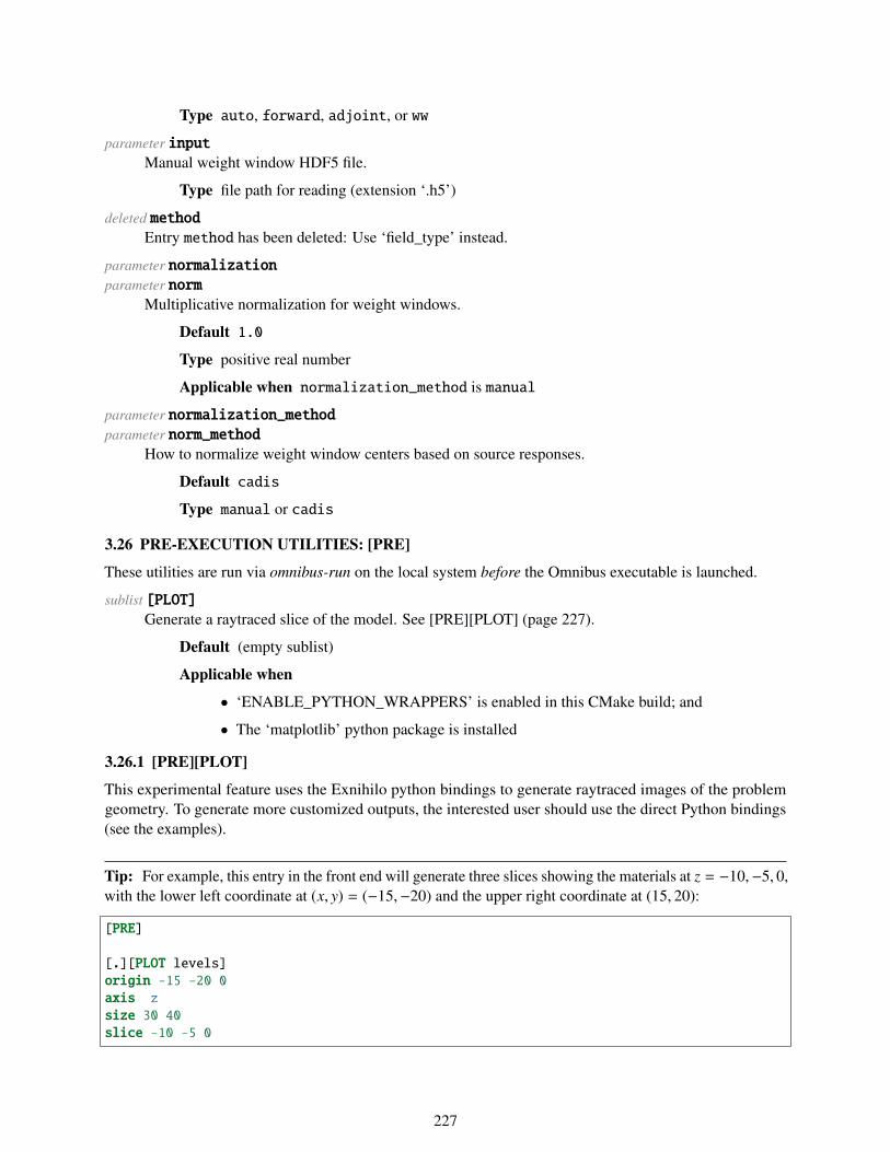
Type auto, forward, adjoint, or ww
parameter inputManual weight window HDF5 file.
Type file path for reading (extension ‘.h5’)
deleted methodEntry method has been deleted: Use ‘field_type’ instead.
parameter normalizationparameter norm
Multiplicative normalization for weight windows.
Default 1.0
Type positive real number
Applicable when normalization_method is manual
parameter normalization_methodparameter norm_method
How to normalize weight window centers based on source responses.
Default cadis
Type manual or cadis
3.26 PRE-EXECUTION UTILITIES: [PRE]
These utilities are run via omnibus-run on the local system before the Omnibus executable is launched.
sublist [PLOT]Generate a raytraced slice of the model. See [PRE][PLOT] (page 227).
Default (empty sublist)
Applicable when
• ‘ENABLE_PYTHON_WRAPPERS’ is enabled in this CMake build; and
• The ‘matplotlib’ python package is installed
3.26.1 [PRE][PLOT]
This experimental feature uses the Exnihilo python bindings to generate raytraced images of the problemgeometry. To generate more customized outputs, the interested user should use the direct Python bindings(see the examples).
Tip: For example, this entry in the front end will generate three slices showing the materials at z = −10,−5, 0,with the lower left coordinate at (x, y) = (−15,−20) and the upper right coordinate at (15, 20):
[PRE]
[.][PLOT levels]origin -15 -20 0axis zsize 30 40slice -10 -5 0
227

parameter axisAxis orthogonal to the image.
Default 2
Type axis (‘x’,’y’,’z’)
parameter checkUse error checking during raytrace.
Default False
Type boolean
parameter cmap(advanced)Color map for plotting.
Default rainbow if trace cell else Set3
Type string without special characters
parameter nameBase name of the output file.
Default plotNNN
Type string without special characters
parameter originLower-left corner of the image.
Units cm
Type length-3 float vector (each element is a real number)
parameter renderSave as a standalone rendered PNG.
Default False
Type boolean
Applicable when The ‘PIL’ python package is installed
parameter resolutionMaximum number of pixels along one axis of the image.
Default 1024
Type positive integer
parameter sizeWidth and height of the image slice.
Units cm
Type pair of floats (each element is a positive real number)
parameter slicePositions along ‘axis’ to take slices, relative to ‘origin.’
228

Default 0.0
Type non-empty float list (each element is a real number)
parameter traceModel property to raytrace.
Default mat
Type cell or mat
3.27 POST-PROCESSING: [POST]
The [POST] block controls post-processing of Omnibus output. It extracts data from the HDF5 output fileand formats it to be more human-accessible.
database [DENOVO]Denovo post-processing options. See [POST][DENOVO] (page 230).
Default (empty database)
Applicable when solver is ‘denovo’
database [DEPLETION]Depletion post-processing options. See [POST][DEPLETION] (page 231).
Default (empty database)
Applicable when solver is ‘depletion’
parameter htmlConvert the ReStructured Text problem summary to HTML.
Default False
Type boolean
Applicable when rst is True
database [HYBRID]Shift post-processing options. See [POST][HYBRID] (page 231).
Default (empty database)
Applicable when problem mode is hybrid
parameter rstWrite a ReStructured Text problem summary.
Default True
Type boolean
database [TALLY]Tally post-processing options. See [POST][TALLY] (page 230).
Default (empty database)
Applicable when
• solver is ‘shift’; and
• /shift/do_transport is True
229

3.27.1 [POST][TALLY]
Tally post-processing options.
parameter cell_csvGenerate CSV files from cell tallies.
Default True
Type boolean
parameter kcode_plotsGenerate keff and convergence plots.
Default True
Type boolean
Applicable when problem mode is kcode
parameter max_csv_size(advanced)Maximum allowed size of average CSV output file.
Default 500.0
Units kB
Type positive real number
Applicable when cell_csv is True
parameter mesh_xdmfGenerate XDMF files from mesh tallies.
Default True
Type boolean
3.27.2 [POST][DENOVO]
Denovo post-processing options.
sublist [SPECTRUM]Save spectra from a list of x/y/z points. See [POST][DENOVO][SPECTRUM] (page 231).
Default (empty sublist)
Applicable when /denovo/disable is none
parameter xdmfCreate an XDMF file for visualization.
Default True
Type boolean
Applicable when /denovo/disable is none
230

3.27.3 [POST][HYBRID]
Shift post-processing options.
parameter ww_xdmfCreate an XDMF file for weight windows.
Default True
Type boolean
Applicable when /shift/vr/output is True
3.27.4 [POST][DEPLETION]
Depletion post-processing options.
parameter max_csv_size(advanced)Maximum allowed size of average CSV output file.
Default 500.0
Units kB
Type positive real number
Applicable when nd_csv is True or xs_csv is True
parameter nd_csvWrite Excel-compatible CSV files with number densities.
Default True
Type boolean
parameter xs_csvWrite CSV files with cross sections.
Default True
Type boolean
Applicable when /depletion/write_xs is True
3.27.5 [POST][DENOVO][SPECTRUM]
Save spectra from a list of x/y/z points.
parameter fieldOutput field from which to save spectra.
Default flux
Type flux, source, or uncflux
postprocessorThe requested field must be enabled in the Denovo output block.
parameter nameShort title or label for the source.
Default spectrumNNN
231

Type string without special characters
parameter normalizationConstant multiplicative factor to apply to spectra.
Default 1.0
Type positive real number
parameter on_disk(advanced)Refrain from loading the solution into memory.
Default False
Type boolean
parameter pointsList of x/y/z points.
Type List of space-separated x/y/z tuples (each element is a real number)
232

4. GEOMETRIA INPUT DESCRIPTION
The Geometria input format is identical to the Omnibus input format and is split into a hierarchy of blocks.All input blocks are described in the following sections.
Note: This documentation was generated automatically with the following version of Exnihilo:
version 6.3.pre-b13 (branch ‘master’ on ‘upstream’, r729: #9809b44f on 2020JUL16)
date 2020-07-16 22:02:43
4.1 GEOMETRIA INPUT FILE CONTENTS
Each of the top-level blocks (and the overall problem input file) are described here.
database [GEOMETRY]Global geometry options. See [GEOMETRY] (page 233).
sublist [UNIVERSE]Universes. See [UNIVERSE] (page 234).
postprocessorUniverse names in /geometry/global must already have been defined.
4.1.1 [GEOMETRY]
Global geometry options.
parameter check_overlapping_volumesPerform extra (and slow) geometry validation checks during transport.
Default False
Type boolean
parameter compositionparameter comp
Provide an optional explicit mapping for composition names.
Default ---
Type list in which each element is a string
command compsMap ‘comp’ to ‘matid’ from pairs or arrow-separated items.
Creates comp
Creates matid
parameter deduplication_warningparameter dedupe_warn
Warn about duplicate surfaces being elided.
Default False
233

Type boolean
parameter globalName of the global universe.
Type string without special characters
parameter length_scaleCharacteristic length scale of the problem.
Default 1.0
Type positive real number
parameter matidMatids corresponding to the given commposition names.
Default ---
Type list in which each element is a non-negative integer
postprocessorThe parameters composition and matid must have the same length.
parameter toleranceparameter tol
Global tolerance for geometry construction and particle bumping.
Default 1e-08
Type real number inside (0, 1)
parameter write_kdtree(advanced)Output the k-D tree representation for each universe.
Default False
Type boolean
4.2 UNIVERSE DEFINITIONS: [UNIVERSE]
Universes are analogous to ‘units’ in KENO: an independent, complete definition of the problem within someregion of space. Universes can be reused multiple times via holes (page 243) and arrays (page 237).
Table 38: Available types for the [UNIVERSE] database
Type Description Applicability
general (page 235) General universekeno6 (page 235) KENO6 universerandom (page 237) Randomly constructed universearray (page 237) Rectangular arrayhexarray (page 239) Hexagonal arraydodarray (page 241) Dodecahedral arrayrtk (page 242) Insert an RTK geometry from an external filecore (page 243) Insert a VERA-defined reactor corertkarray Alias to rtk type —
234

4.2.1 [UNIVERSE=GENERAL]
The “general” universe is a constructive solid geometry universe, essentially equivalent to a “unit” in KENO.Its components are “cells”, solid bodies with a single fill material, and “holes”, which are other universesembedded into this general universe.
command boundaryCreate an interior parameter for a single bounding shape.
Creates interior
sublist [CELL]Cell definition. See [UNIVERSE][CELL] (page 244).
Default (empty sublist)
sublist [HOLE]Inserted sub-universes. See [UNIVERSE][HOLE] (page 243).
Optional
parameter interiorSenses and shape names defining the interior of this universe.
Type list in which each element is a shape with optional leading +- sense
postprocessorCheck that interior shapes have been defined.
parameter nameName of the universe.
Type string without special characters
sublist [SHAPE]Geometry shapes. See [UNIVERSE][SHAPE] (page 246).
Default (empty sublist)
4.2.2 [UNIVERSE=KENO6]
The “KENO” universe activates features necessary to build KENO geometry definitions using GG. UnlikeGG, KENO continually tracks on many geometry layers simultaneously, so that the “topmost” layer’s cellsare used. This allows holes and arrays to be defined without integrating them into the daughter universes –they simply override whatever is there.
GG’s tracking engine operates differently: it tracks on only one universe at a time, so that in any universe, asingle point in space corresponds to exactly one logical position in that universe, or else it is in the “exterior”of that universe. Particles hitting the exterior are transported to another universe (except in the outermostuniverse where the boundary condition is applied).
To unify these two tracking types, this special universe uses intersection tests to automatically modify the celldefinitions. It uses shape-to-shape intersection tests to determine whether any of the specified holes, arrays,or external boundaries modify the cells interior to the problem. The test for shape A intersecting shape B canreturn one of five results:
Separate A and B do not intersect.
235

Identical A and B are exactly the same shape: their logical definition and surfaces are identical.
Encloses The region in A is a superset of the region of B
Enclosed by The region in B is a superset of the region of A
Overlaps The two regions may intersect (or one may even enclose the other). This result increases geometrycomplexity but is the most conservative.
Some of the shape-to-shape intersection tests are more accurate than others. Spheres, aligned cylinders,cuboids, and planes can tell their exact relationship to shapes of the same kind, but it’s not always possible totell the exact intersection result for some shapes. The conservative case extends cell definitions to exclude theshapes in question.
sublist [ARRAY]Implicitly truncated arrays. See [UNIVERSE][ARRAY] (page 244).
Optional
command boundaryCreate an interior parameter for a single bounding shape.
Creates interior
sublist [CELL]Cell definition. See [UNIVERSE][CELL] (page 244).
Default (empty sublist)
sublist [HOLE]Inserted sub-universes. See [UNIVERSE][HOLE] (page 243).
Optional
parameter interiorSenses and shape names defining the interior of this universe.
Type list in which each element is a shape with optional leading +- sense
postprocessorCheck that interior shapes have been defined.
parameter nameName of the universe.
Type string without special characters
sublist [SHAPE]Geometry shapes. See [UNIVERSE][SHAPE] (page 246).
Default (empty sublist)
236

4.2.3 [UNIVERSE=RANDOM]
The “random” universe is a procedurally generated universe filled with a given volume fraction of spheres. Itis used for HTGRs to model pebbles and TRISO particles.
It is defined by specifying one or more previously defined spherical universes (e.g. particles with differentcompositions) that will be replicated inside the universe. The number of embedded particles is determined byspecifying a volume fraction v such that Ni =
vfiVTVi
for particle type i which has volume Vi inside an object ofvolume Vt.
The region outside the sampled particles is filled with the single composition composition. (If the randomuniverse is a fuel pebble and the particles are TRISO particles, this composition will be the graphite matrix.)
Currently, the only shapes supported as bounding shapes are a single cuboid, sphere, and cylinder withoutany rotations or translations applied.
parameter compositionparameter comp
Composition outside of the particles (the matrix).
Type non-empty string
parameter fillNames of particle universes to emplace.
Type list in which each element is a string without special characters
postprocessorUniverse names in fill must already have been defined.
parameter nameName of the universe.
Type string without special characters
database [OPTIONS]Random universe construction options. See [UNIVERSE][OPTIONS] (page 245).
database [SHAPE]Geometry shapes. See [UNIVERSE][SHAPE] (page 246).
parameter volume_fractionparameter vf
Names of particle universes to emplace.
Type fractions that sum to less than one (each element is a real number inside (0, 1))
4.2.4 [UNIVERSE=ARRAY]
Rectangular array.
command boundaryCreate an interior parameter for a single bounding shape.
Creates interior
parameter clip_composition
237

parameter clipComposition that will replace any clipped array cell.
Optional
Type non-empty string
parameter fillNames of array universe fills, indexed as ZUV.
Type list in which each element is a string without special characters
postprocessorUniverse names in fill must already have been defined.
sublist [HOLE]Inserted sub-universes. See [UNIVERSE][HOLE] (page 243).
Optional
parameter interiorSense/shapes defining the interior of the array.
Optional
Type list in which each element is a shape with optional leading +- sense
postprocessorCheck that interior shapes have been defined.
parameter nameName of the universe.
Type string without special characters
parameter nxNumber of units in the X direction.
Type positive integer
parameter nyNumber of units in the Y direction.
Type positive integer
parameter nzNumber of units in the Z direction.
Default 1
Type positive integer
postprocessorCheck array sizes.
parameter originLocation of the lower-left corner of the array bounds.
Default 0.0 0.0 0.0
Type length-3 float vector (each element is a real number)
238

parameter origin_isWhether origin is the array lower-left or a unit origin.
Default ‘array’ unless the ‘place’ parameter is present
Type array or unit
parameter placeLocation of the lower-left corner of the array bounds.
Type length-3 logical position vector (each element is a non-negative integer)
Applicable when origin_is is unit
sublist [SHAPE]Geometry shapes. See [UNIVERSE][SHAPE] (page 246).
Default (empty sublist)
4.2.5 [UNIVERSE=HEXARRAY]
Hexagonal array.
command boundaryCreate an interior parameter for a single bounding shape.
Creates interior
parameter clip_compositionparameter clip
Composition that will replace any clipped array cell.
Optional
Type non-empty string
parameter fillNames of array universe fills, indexed as ZUV.
Type list in which each element is a string without special characters
postprocessorUniverse names in fill must already have been defined.
sublist [HOLE]Inserted sub-universes. See [UNIVERSE][HOLE] (page 243).
Optional
parameter interiorSense/shapes defining the interior of the array.
Type list in which each element is a shape with optional leading +- sense
postprocessorCheck that interior shapes have been defined.
parameter layoutLayout of the hex array elements.
239

Default rhomb
Type rhomb or rect
parameter nameName of the universe.
Type string without special characters
parameter nuNumber of units in the U direction.
Type positive integer
parameter nvNumber of units in the V direction.
Type positive integer
parameter nzNumber of units in the Z direction.
Default 1
Type positive integer
postprocessorCheck array sizes.
parameter originLocation of the lower-left corner of the array bounds.
Default 0.0 0.0 0.0
Type length-3 float vector (each element is a real number)
parameter origin_isWhether origin is the array lower-left or a unit origin.
Default ‘array’ unless the ‘place’ parameter is present
Type array or unit
parameter placeLocation of the lower-left corner of the array bounds.
Type length-3 logical position vector (each element is a non-negative integer)
Applicable when origin_is is unit
sublist [SHAPE]Geometry shapes. See [UNIVERSE][SHAPE] (page 246).
Default (empty sublist)
240

4.2.6 [UNIVERSE=DODARRAY]
Dodecahedral array.
command boundaryCreate an interior parameter for a single bounding shape.
Creates interior
parameter clip_compositionparameter clip
Composition that will replace any clipped array cell.
Optional
Type non-empty string
parameter fillNames of array universe fills, indexed as ZUV.
Type list in which each element is a string without special characters
postprocessorUniverse names in fill must already have been defined.
sublist [HOLE]Inserted sub-universes. See [UNIVERSE][HOLE] (page 243).
Optional
parameter interiorSense/shapes defining the interior of the array.
Type list in which each element is a shape with optional leading +- sense
postprocessorCheck that interior shapes have been defined.
parameter nameName of the universe.
Type string without special characters
parameter nxNumber of units in the X direction.
Type positive integer
parameter nyNumber of units in the Y direction.
Type positive integer
parameter nzNumber of units in the Z direction.
Default 1
Type positive integer
241

postprocessorCheck array sizes.
parameter originLocation of the lower-left corner of the array bounds.
Default 0.0 0.0 0.0
Type length-3 float vector (each element is a real number)
parameter origin_isWhether origin is the array lower-left or a unit origin.
Default ‘array’ unless the ‘place’ parameter is present
Type array or unit
parameter placeLocation of the lower-left corner of the array bounds.
Type length-3 logical position vector (each element is a non-negative integer)
Applicable when origin_is is unit
sublist [SHAPE]Geometry shapes. See [UNIVERSE][SHAPE] (page 246).
Default (empty sublist)
4.2.7 [UNIVERSE=RTK]
Insert an RTK geometry from an external file.
command boundaryCreate an interior parameter for a single bounding shape.
Creates interior
sublist [HOLE]Inserted sub-universes. See [UNIVERSE][HOLE] (page 243).
Optional
parameter inputPath to the RTK geometry XML file.
Type file path for reading (extension ‘.xml’)
parameter interiorSense/shapes defining the interior of the array.
Type list in which each element is a shape with optional leading +- sense
postprocessorCheck that interior shapes have been defined.
parameter nameName of the universe.
Type string without special characters
sublist [SHAPE]Geometry shapes. See [UNIVERSE][SHAPE] (page 246).
Default (empty sublist)
242

4.2.8 [UNIVERSE=CORE]
The core universe can only be used when running a VERA (Virtual Environment for Reactor Applications)model in Omnibus or when run externally through the VERA code suite. It inserts the analyst-defined reactordesign into a Geometria input for external dosimetry applications.
parameter nameName of universe.
Type string without special characters
4.2.9 [UNIVERSE][HOLE]
Inserted sub-universes.
command eulerPerform an Euler rotation about the z, x′, z′′ axes.
Units revolution
Creates rotate
parameter fillName of the universe to fill this hole with.
Type string without special characters
postprocessorUniverse names in fill must already have been defined.
parameter nameName of the shape that this hole creates.
Type string without special characters
parameter rotateRotation matrix.
Default 1.0 0.0 0.0 0.0 1.0 0.0 0.0 0.0 1.0
Type length-9 row-major rotation matrix (each element is a real number)
postprocessor (advanced)Squelch identity rotations and null translations.
parameter translateLocal-to-global translation vector.
Default 0.0 0.0 0.0
Type length-3 float vector (each element is a real number)
243

4.2.10 [UNIVERSE][CELL]
Cells are defined as the intersection of one or more regions defined by shapes and holes. Each shape separatesspace into two half-spaces: “inside” the shape, with a “negative” sense, and “outside” the shape with a“positive” sense. For a shape called sphere, these two senses are written as -sphere (inside) and +sphere(outside). When another universe is placed into this general universe via a hole, it implicitly creates a shape –the external boundary of the embedded universe – that can be referenced when defining cells.
The choice for the signs is based on the standard form of the quadric equations, such as the surface of asphere:
x2 + y2 + z2 − R2 = 0
When the left-hand side of this equation is positive (+), the point (x, y, z) is outside the sphere; when negative(-), the point is inside. We think of surfaces and shapes as having outward-facing normals; when the projectionof a point onto the surface is negative, the point is inside.
parameter compositionparameter comp
Name of the composition that fills this cell.
Type non-empty string
deleted matidEntry matid has been deleted: ‘matid’ has been replaced with ‘comp’, the name of the composition.
parameter nameName of the cell.
Type string without special characters
parameter shapesSenses and shape names defining this cell.
Type list in which each element is a shape with optional leading +- sense
postprocessorCheck that shapes have been defined.
parameter volumeAdd a pre-calculated volume for this cell.
Optional
Type real number
4.2.11 [UNIVERSE][ARRAY]
Implicitly truncated arrays.
command eulerPerform an Euler rotation about the z, x′, z′′ axes.
Units revolution
Creates rotate
244

parameter fillName of the universe to fill this hole with.
Type string without special characters
postprocessorUniverse names in fill must already have been defined.
parameter nameName of the shape that this hole creates.
Type string without special characters
parameter rotateRotation matrix.
Default 1.0 0.0 0.0 0.0 1.0 0.0 0.0 0.0 1.0
Type length-9 row-major rotation matrix (each element is a real number)
postprocessor (advanced)Squelch identity rotations and null translations.
parameter translateLocal-to-global translation vector.
Default 0.0 0.0 0.0
Type length-3 float vector (each element is a real number)
4.2.12 [UNIVERSE][OPTIONS]
Random universe construction options.
parameter failure_batch_sizeNumber of samples per batch to test.
Default 100000
Type positive integer
parameter failure_toleranceFraction of samples per batch that must be rejected to fail.
Default 0.99999
Type real number inside (0, 1)
parameter insert_methodMethod for attempting to insert particles into a pebble.
The naive method is the simplest and slowest way to instantiate a loosely packed particle universe. Itsamples random points inside the universe and rejects them if the sphere around that particle intersectswith any particle previously sampled. The naive collision detection scales with O(N2) for N particles,and the rejection fraction approaches 1 very quickly.
When sampling with the naive method, batches of failure_batch_size samples are tallied; if thefraction of failed samples exceeds failure_tolerance then an error will be raised.
Default naive
245

Type naive
parameter seedSeed value for instantiating this universe.
The seed is used to choose an independent random number stream when instantiating a universe.Different universes’ particle placements will be uncorrelated even if they share a seed, but changingthe universe’s name will change the particle placements, as the actual computational seed value is acombination of the seed given by this parameter and the name of this universe.
Default 0
Type non-negative integer
4.3 SHAPE DEFINITIONS: [UNIVERSE][SHAPE]
Shapes are primitive solid bodies, the constituents of cells. Although this manual does not yet include helpfulimages for the shape descriptions, the KENO-VI shape description section of the SCALE user manual [2] isessentially equivalent to the input quantities in Geometria. For example, the wedge construction examplegives wedge label xbase xpt ypt zlng, and the wedge input block (page 256) defines zlng as an aliasfor height, xbase as an alias for width, and xy as an alias for corner_pt.
Each shape is the intersection of half-spaces defined by primitive quadric surfaces. When a geometryis instantiated, the shapes are decomposed into their surfaces and volumes are expressed by a logicalrepresentation of these surfaces using boolean logic as is typical with a constructive solid geometry definition.
The coordinate system of the shape is defined using a rotation matrix and translation vector: rotations areapplied to the shape about its origin, then translations moves the daughter shape relative to the parent universe.The transformation from a point in the shape’s coordinate system into the universe’s system is
xu = Rxs + t ,
Where the subscripts u, s refer to the universe and shape coordinate systems, respectively. The vector t is atranslation vector. To transform from the parent into the daughter system we apply the inverse:
xs = RT (xu − t) .
(Note that because R is unitary, the transpose is equal to the inverse.)
The surfaces created by each shape have unique names that can be used to reference them later, or to createreflecting outer boundaries during construction.
Most shapes share many of the same parameters such as “reflect” and “rotate”. To reduce duplication, themore detailed documentation is provided for the “cuboid” shape:
• euler (page 247)
• rotate (page 248)
• reflect (page 248)
Table 39: Available types for the [SHAPE] database
246

Type Description Applicability
cuboid (page 247) Box shapebox Alias to cuboid type —sphere (page 249) Sphere shapecyl (page 250) Cylinder shapecylsegment (page 251) Cylinder segment shapepad Alias to cylsegment type —ring (page 252) Cylindrical shell shapecylshell Alias to ring type —prism (page 253) Regular prism shapeslab (page 255) Infinite slab shapeplane (page 255) Infinite half-spacewedge (page 256) Wedge shapecone (page 257) Cone shapeellipsoid (page 258) Ellipsoid shapehopper (page 259) Hopper shaperighttet (page 260) Right tetrahedron shapetriprism (page 261) Triangular prism shapeecylinder (page 261) Elliptical cylinder shaperhombdod (page 262) Rhombic dodecahedron shapeppiped (page 263) Parallelepipedquadric (page 264) General quadric
4.3.1 [UNIVERSE][SHAPE=CUBOID]
The possible reflecting faces for the cuboid (chosen via reflect) are:
Face Description
mx lower x facepx upper x facemy lower y facepy upper y facemz lower z facepz upper z face
command eulerPerform an Euler rotation about the z, x′, z′′ axes.
See [the Euler angles wikipedia page](https://en.wikipedia.org/wiki/Euler_angles#Definition_by_intrinsic_rotations) for a graphic representation of the z, x′, z′′ rotation. This command simply generatesa rotation matrix.
Units revolution
Creates rotate
command facesExpand into parameters xmin, xmax, ymin, ymax, zmin, and zmax.
247

Creates xmin
Creates xmax
Creates ymin
Creates ymax
Creates zmin
Creates zmax
parameter nameName of the shape.
Type string without special characters
parameter reflectReflecting boundary surfaces.
The reflect option allows a subset of faces on a shape to specularly reflect particles. Enter the singlevalue * to reflect all faces for the given shape.
Default ---
Type list of shape surfaces (e.g. mx, co) (each element is a string without special characters)
parameter rotateRotation matrix.
The rotation matrix
R =
⎡⎢⎢⎢⎢⎢⎢⎢⎢⎣a b cd e fg h i
⎤⎥⎥⎥⎥⎥⎥⎥⎥⎦is applied to a point in the shape’s coordinate system as a column vector
Rxs = R
⎡⎢⎢⎢⎢⎢⎢⎢⎢⎣xyz
⎤⎥⎥⎥⎥⎥⎥⎥⎥⎦The input to the code is the row-major flattened list [a, b, c, d, e, f , g, h, i].
Default 1.0 0.0 0.0 0.0 1.0 0.0 0.0 0.0 1.0
Type length-9 row-major rotation matrix (each element is a real number)
postprocessor (advanced)Squelch identity rotations and null translations.
parameter translateparameter origin
Local-to-global translation vector.
Default 0.0 0.0 0.0
Type length-3 float vector (each element is a real number)
248

parameter xmaxMaximum x-coordinate of box source.
Type real number
postprocessorParameter xmin must be less than xmax.
parameter xminMinimum x-coordinate of box source.
Type real number
parameter ymaxMaximum y-coordinate of box source.
Type real number
postprocessorParameter ymin must be less than ymax.
parameter yminMinimum y-coordinate of box source.
Type real number
parameter zmaxMaximum z-coordinate of box source.
Type real number
postprocessorParameter zmin must be less than zmax.
parameter zminMinimum z-coordinate of box source.
Type real number
4.3.2 [UNIVERSE][SHAPE=SPHERE]
Sphere shape.
command eulerPerform an Euler rotation about the z, x′, z′′ axes.
Units revolution
Creates rotate
parameter nameName of the shape.
Type string without special characters
parameter radiusparameter r
Radius of sphere.
Type real number
249

parameter reflectReflecting boundary surfaces.
Default ---
Type list of shape surfaces (e.g. mx, co) (each element is a string without special characters)
parameter rotateRotation matrix.
Default 1.0 0.0 0.0 0.0 1.0 0.0 0.0 0.0 1.0
Type length-9 row-major rotation matrix (each element is a real number)
postprocessor (advanced)Squelch identity rotations and null translations.
parameter translateparameter origin
Local-to-global translation vector.
Default 0.0 0.0 0.0
Type length-3 float vector (each element is a real number)
4.3.3 [UNIVERSE][SHAPE=CYL]
Cylinder shape.
parameter axisAxis along the cylinder.
Type axis (‘x’,’y’,’z’)
command eulerPerform an Euler rotation about the z, x′, z′′ axes.
Units revolution
Creates rotate
parameter extentsNegative and positive position along the given axis.
Type (min, max) extent values (each element is a real number)
parameter nameName of the shape.
Type string without special characters
parameter radiusparameter r
Radius of cylinder.
Type real number
parameter reflectReflecting boundary surfaces.
250

Default ---
Type list of shape surfaces (e.g. mx, co) (each element is a string without special characters)
parameter rotateRotation matrix.
Default 1.0 0.0 0.0 0.0 1.0 0.0 0.0 0.0 1.0
Type length-9 row-major rotation matrix (each element is a real number)
postprocessor (advanced)Squelch identity rotations and null translations.
parameter translateparameter origin
Local-to-global translation vector.
Default 0.0 0.0 0.0
Type length-3 float vector (each element is a real number)
4.3.4 [UNIVERSE][SHAPE=CYLSEGMENT]
Cylinder segment shape.
parameter angleparameter a
Beginning angle CCW from x = 0.
Units revolution
Type real number inclusive [0.0, 1.0]
parameter arcparameter da
Angle subtended by cylindrical segment.
Units revolution
Type real number in [0.0, 0.5]
deleted begin_angledeleted ba
Entry begin_angle has been deleted: Replaced by ‘angle’ in turns not radians.
command eulerPerform an Euler rotation about the z, x′, z′′ axes.
Units revolution
Creates rotate
parameter extentsNegative and positive position along the z-axis.
Type (min, max) extent values (each element is a real number)
parameter inner_radius
251

parameter riInner radius.
Type positive real number
parameter nameName of the shape.
Type string without special characters
parameter outer_radiusparameter ro
Outer radius.
Type positive real number
postprocessorParameter inner_radius must be less than outer_radius.
parameter reflectReflecting boundary surfaces.
Default ---
Type list of shape surfaces (e.g. mx, co) (each element is a string without special characters)
parameter rotateRotation matrix.
Default 1.0 0.0 0.0 0.0 1.0 0.0 0.0 0.0 1.0
Type length-9 row-major rotation matrix (each element is a real number)
postprocessor (advanced)Squelch identity rotations and null translations.
deleted solid_angledeleted sa
Entry solid_angle has been deleted: Replaced by ‘arc’ in turns not radians.
parameter translateparameter origin
Local-to-global translation vector.
Default 0.0 0.0 0.0
Type length-3 float vector (each element is a real number)
4.3.5 [UNIVERSE][SHAPE=RING]
Cylindrical shell shape.
command eulerPerform an Euler rotation about the z, x′, z′′ axes.
Units revolution
Creates rotate
252

parameter extentsNegative and positive position along the Z axis.
Type (min, max) extent values (each element is a real number)
parameter inner_radiusparameter ri
Inner radius.
Type real number
parameter nameName of the shape.
Type string without special characters
parameter outer_radiusparameter ro
Outer radius.
Type real number
postprocessorParameter inner_radius must be less than outer_radius.
parameter reflectReflecting boundary surfaces.
Default ---
Type list of shape surfaces (e.g. mx, co) (each element is a string without special characters)
parameter rotateRotation matrix.
Default 1.0 0.0 0.0 0.0 1.0 0.0 0.0 0.0 1.0
Type length-9 row-major rotation matrix (each element is a real number)
postprocessor (advanced)Squelch identity rotations and null translations.
parameter translateparameter origin
Local-to-global translation vector.
Default 0.0 0.0 0.0
Type length-3 float vector (each element is a real number)
4.3.6 [UNIVERSE][SHAPE=PRISM]
The possible reflecting faces for a prism depend on the number of sides:
Face Description
pN for integer N in [0, num_sides), CCW from x=0mz lower z facepz upper z face
253

parameter apothemparameter r
Inner radius of the prism.
Type real number
command eulerPerform an Euler rotation about the z, x′, z′′ axes.
Units revolution
Creates rotate
parameter extentsNegative and positive position along the Z axis.
Type (min, max) extent values (each element is a real number)
parameter nameName of the shape.
Type string without special characters
parameter num_sidesNumber of sides on the prism.
Type integer >= 3
parameter reflectReflecting boundary surfaces.
Default ---
Type list of shape surfaces (e.g. mx, co) (each element is a string without special characters)
parameter rotateRotation matrix.
Default 1.0 0.0 0.0 0.0 1.0 0.0 0.0 0.0 1.0
Type length-9 row-major rotation matrix (each element is a real number)
postprocessor (advanced)Squelch identity rotations and null translations.
parameter rotfracAngle (fraction of the angle spanned by one face) to rotate.
Default 0.0
Type real number inclusive [0.0, 1.0]
parameter translateparameter origin
Local-to-global translation vector.
Default 0.0 0.0 0.0
Type length-3 float vector (each element is a real number)
254

4.3.7 [UNIVERSE][SHAPE=SLAB]
Infinite slab shape.
parameter axisAxis along the slab.
Type axis (‘x’,’y’,’z’)
command eulerPerform an Euler rotation about the z, x′, z′′ axes.
Units revolution
Creates rotate
parameter extentsNegative and positive position along the slab axis.
Type (min, max) extent values (each element is a real number)
parameter nameName of the shape.
Type string without special characters
parameter reflectReflecting boundary surfaces.
Default ---
Type list of shape surfaces (e.g. mx, co) (each element is a string without special characters)
parameter rotateRotation matrix.
Default 1.0 0.0 0.0 0.0 1.0 0.0 0.0 0.0 1.0
Type length-9 row-major rotation matrix (each element is a real number)
postprocessor (advanced)Squelch identity rotations and null translations.
parameter translateparameter origin
Local-to-global translation vector.
Default 0.0 0.0 0.0
Type length-3 float vector (each element is a real number)
4.3.8 [UNIVERSE][SHAPE=PLANE]
Infinite half-space.
command eulerPerform an Euler rotation about the z, x′, z′′ axes.
Units revolution
Creates rotate
255

parameter nameName of the shape.
Type string without special characters
parameter normalVector (possibly unnormalized) point outward from the plane.
Type length-3 float vector (each element is a real number)
parameter pointA point somewhere on the plane.
Type length-3 float vector (each element is a real number)
parameter reflectReflecting boundary surfaces.
Default ---
Type list of shape surfaces (e.g. mx, co) (each element is a string without special characters)
parameter rotateRotation matrix.
Default 1.0 0.0 0.0 0.0 1.0 0.0 0.0 0.0 1.0
Type length-9 row-major rotation matrix (each element is a real number)
postprocessor (advanced)Squelch identity rotations and null translations.
parameter translateparameter origin
Local-to-global translation vector.
Default 0.0 0.0 0.0
Type length-3 float vector (each element is a real number)
4.3.9 [UNIVERSE][SHAPE=WEDGE]
Wedge shape.
parameter corner_ptparameter xy
XY location of the right-angle corner of the wedge.
Type length-2 (x,y) position (each element is a positive real number)
command eulerPerform an Euler rotation about the z, x′, z′′ axes.
Units revolution
Creates rotate
parameter heightparameter zlng
Height of the wedge (along Z axis).
256

Type positive real number
parameter nameName of the shape.
Type string without special characters
parameter reflectReflecting boundary surfaces.
Default ---
Type list of shape surfaces (e.g. mx, co) (each element is a string without special characters)
parameter rotateRotation matrix.
Default 1.0 0.0 0.0 0.0 1.0 0.0 0.0 0.0 1.0
Type length-9 row-major rotation matrix (each element is a real number)
postprocessor (advanced)Squelch identity rotations and null translations.
parameter translateparameter origin
Local-to-global translation vector.
Default 0.0 0.0 0.0
Type length-3 float vector (each element is a real number)
parameter widthparameter xbase
Length of the hypotenuse of the wedge (along the X axis).
Type positive real number
4.3.10 [UNIVERSE][SHAPE=CONE]
Cone shape.
parameter axisAxis along the centerline of the cone.
Type axis (‘x’,’y’,’z’)
command eulerPerform an Euler rotation about the z, x′, z′′ axes.
Units revolution
Creates rotate
parameter extentsNegative and positive base positions along the given axis.
Type (min, max) extent values (each element is a real number)
parameter nameName of the shape.
257

Type string without special characters
parameter radiiparameter r
Radii at the top and bottom.
Type 2 positive floats (each element is a positive real number)
parameter reflectReflecting boundary surfaces.
Default ---
Type list of shape surfaces (e.g. mx, co) (each element is a string without special characters)
parameter rotateRotation matrix.
Default 1.0 0.0 0.0 0.0 1.0 0.0 0.0 0.0 1.0
Type length-9 row-major rotation matrix (each element is a real number)
postprocessor (advanced)Squelch identity rotations and null translations.
parameter translateparameter origin
Local-to-global translation vector.
Default 0.0 0.0 0.0
Type length-3 float vector (each element is a real number)
4.3.11 [UNIVERSE][SHAPE=ELLIPSOID]
Ellipsoid shape.
command eulerPerform an Euler rotation about the z, x′, z′′ axes.
Units revolution
Creates rotate
parameter nameName of the shape.
Type string without special characters
parameter radiiparameter r
Radii in the x, y, and z directions.
Type 3 positive floats (each element is a positive real number)
parameter reflectReflecting boundary surfaces.
Default ---
258

Type list of shape surfaces (e.g. mx, co) (each element is a string without special characters)
parameter rotateRotation matrix.
Default 1.0 0.0 0.0 0.0 1.0 0.0 0.0 0.0 1.0
Type length-9 row-major rotation matrix (each element is a real number)
postprocessor (advanced)Squelch identity rotations and null translations.
parameter translateparameter origin
Local-to-global translation vector.
Default 0.0 0.0 0.0
Type length-3 float vector (each element is a real number)
4.3.12 [UNIVERSE][SHAPE=HOPPER]
Hopper shape.
command eulerPerform an Euler rotation about the z, x′, z′′ axes.
Units revolution
Creates rotate
parameter extentsNegative and positive base positions along the Z axis.
Type (min, max) extent values (each element is a real number)
parameter lower_ptparameter lo
X and Y half-lengths on the low side of the hopper.
Type length-2 (x,y) position (each element is a positive real number)
parameter nameName of the shape.
Type string without special characters
parameter reflectReflecting boundary surfaces.
Default ---
Type list of shape surfaces (e.g. mx, co) (each element is a string without special characters)
parameter rotateRotation matrix.
Default 1.0 0.0 0.0 0.0 1.0 0.0 0.0 0.0 1.0
Type length-9 row-major rotation matrix (each element is a real number)
259

postprocessor (advanced)Squelch identity rotations and null translations.
parameter translateparameter origin
Local-to-global translation vector.
Default 0.0 0.0 0.0
Type length-3 float vector (each element is a real number)
parameter upper_ptparameter hi
X and Y half-lengths on the high side of the hopper.
Type length-2 (x,y) position (each element is a positive real number)
4.3.13 [UNIVERSE][SHAPE=RIGHTTET]
Right tetrahedron shape.
command eulerPerform an Euler rotation about the z, x′, z′′ axes.
Units revolution
Creates rotate
parameter lengthsLength of the tetrahedron edges along the x, y, and z axes.
Type 3 positive floats (each element is a positive real number)
parameter nameName of the shape.
Type string without special characters
parameter reflectReflecting boundary surfaces.
Default ---
Type list of shape surfaces (e.g. mx, co) (each element is a string without special characters)
parameter rotateRotation matrix.
Default 1.0 0.0 0.0 0.0 1.0 0.0 0.0 0.0 1.0
Type length-9 row-major rotation matrix (each element is a real number)
postprocessor (advanced)Squelch identity rotations and null translations.
parameter translateparameter origin
Local-to-global translation vector.
Default 0.0 0.0 0.0
Type length-3 float vector (each element is a real number)
260

4.3.14 [UNIVERSE][SHAPE=TRIPRISM]
Triangular prism shape.
command eulerPerform an Euler rotation about the z, x′, z′′ axes.
Units revolution
Creates rotate
parameter lengthsLength of the triangular prism’s bounding box.
Type 3 positive floats (each element is a positive real number)
parameter nameName of the shape.
Type string without special characters
parameter reflectReflecting boundary surfaces.
Default ---
Type list of shape surfaces (e.g. mx, co) (each element is a string without special characters)
parameter rotateRotation matrix.
Default 1.0 0.0 0.0 0.0 1.0 0.0 0.0 0.0 1.0
Type length-9 row-major rotation matrix (each element is a real number)
postprocessor (advanced)Squelch identity rotations and null translations.
parameter translateparameter origin
Local-to-global translation vector.
Default 0.0 0.0 0.0
Type length-3 float vector (each element is a real number)
4.3.15 [UNIVERSE][SHAPE=ECYLINDER]
Elliptical cylinder shape.
command eulerPerform an Euler rotation about the z, x′, z′′ axes.
Units revolution
Creates rotate
parameter extentsNegative and positive position along the given axis.
Type (min, max) extent values (each element is a real number)
261

parameter nameName of the shape.
Type string without special characters
parameter radiiparameter r
Radii in the x and y directions.
Type length-2 (x,y) position (each element is a positive real number)
parameter reflectReflecting boundary surfaces.
Default ---
Type list of shape surfaces (e.g. mx, co) (each element is a string without special characters)
parameter rotateRotation matrix.
Default 1.0 0.0 0.0 0.0 1.0 0.0 0.0 0.0 1.0
Type length-9 row-major rotation matrix (each element is a real number)
postprocessor (advanced)Squelch identity rotations and null translations.
parameter translateparameter origin
Local-to-global translation vector.
Default 0.0 0.0 0.0
Type length-3 float vector (each element is a real number)
4.3.16 [UNIVERSE][SHAPE=RHOMBDOD]
The faces of a rhombic dodecahedron are ordered so that face n connects to n + 6 mod 12 of an adjacentlattice cell. For a dodecahedron with interior radius 1, these faces are:
Face Description
px Plane: x=1py Plane: y=1p0 Plane: n=(0.5 0.5 0.707107), d=1p1 Plane: n=(0.5 -0.5 -0.707107), d=-1p2 Plane: n=(0.5 -0.5 0.707107), d=1p3 Plane: n=(0.5 0.5 -0.707107), d=-1mx Plane: x=-1my Plane: y=-1p4 Plane: n=(0.5 0.5 0.707107), d=-1p5 Plane: n=(0.5 -0.5 -0.707107), d=1p6 Plane: n=(0.5 -0.5 0.707107), d=-1p7 Plane: n=(0.5 0.5 -0.707107), d=1
262

parameter apothemparameter r
Inner radius of the dodecahedron.
Type positive real number
command eulerPerform an Euler rotation about the z, x′, z′′ axes.
Units revolution
Creates rotate
parameter nameName of the shape.
Type string without special characters
parameter reflectReflecting boundary surfaces.
Default ---
Type list of shape surfaces (e.g. mx, co) (each element is a string without special characters)
parameter rotateRotation matrix.
Default 1.0 0.0 0.0 0.0 1.0 0.0 0.0 0.0 1.0
Type length-9 row-major rotation matrix (each element is a real number)
postprocessor (advanced)Squelch identity rotations and null translations.
parameter translateparameter origin
Local-to-global translation vector.
Default 0.0 0.0 0.0
Type length-3 float vector (each element is a real number)
4.3.17 [UNIVERSE][SHAPE=PPIPED]
Parallelepiped.
command eulerPerform an Euler rotation about the z, x′, z′′ axes.
Units revolution
Creates rotate
parameter lengthsLength of the x, xy, and xyz edges.
Type 3 positive floats (each element is a positive real number)
parameter nameName of the shape.
263

Type string without special characters
parameter reflectReflecting boundary surfaces.
Default ---
Type list of shape surfaces (e.g. mx, co) (each element is a string without special characters)
parameter rotateRotation matrix.
Default 1.0 0.0 0.0 0.0 1.0 0.0 0.0 0.0 1.0
Type length-9 row-major rotation matrix (each element is a real number)
postprocessor (advanced)Squelch identity rotations and null translations.
parameter translateparameter origin
Local-to-global translation vector.
Default 0.0 0.0 0.0
Type length-3 float vector (each element is a real number)
parameter xy_angleparameter phi
Angle between xy component of xyz edge and x axis (phi).
Units revolution
Type real number in [0,.25)
parameter xyz_angleparameter theta
Angle between xyz edge and z axis (theta).
Units revolution
Type real number in [0,.25)
parameter y_angleparameter psi
Angle between xy edge and y axis (psi).
Units revolution
Type real number in [0,.25)
4.3.18 [UNIVERSE][SHAPE=QUADRIC]
General quadric.
parameter crossparameter def
Second-order cross coefficients dXY + eYZ + f XZ.
Default 0.0 0.0 0.0
264

Type length-3 float vector (each element is a real number)
command eulerPerform an Euler rotation about the z, x′, z′′ axes.
Units revolution
Creates rotate
parameter firstparameter ghi
First-order coefficients gX + hY + iZ.
Default 0.0 0.0 0.0
Type length-3 float vector (each element is a real number)
parameter nameName of the shape.
Type string without special characters
parameter reflectReflecting boundary surfaces.
Default ---
Type list of shape surfaces (e.g. mx, co) (each element is a string without special characters)
parameter rotateRotation matrix.
Default 1.0 0.0 0.0 0.0 1.0 0.0 0.0 0.0 1.0
Type length-9 row-major rotation matrix (each element is a real number)
postprocessor (advanced)Squelch identity rotations and null translations.
parameter scalarparameter j
Scalar coefficient j.
Default 0.0
Type real number
parameter secondparameter abc
Second-order coefficients aX2 + bY2 + cZ2.
Default 0.0 0.0 0.0
Type length-3 float vector (each element is a real number)
parameter translateparameter origin
Local-to-global translation vector.
Default 0.0 0.0 0.0
Type length-3 float vector (each element is a real number)
265


REFERENCES
[1] Kobayashi, K., Sugimura, N., and Nagaya, Y. 3-D Radiation Transport Benchmark Problems andResults for Simple Geometries with Void Regions. Nuclear Energy Agency, 2000.
[2] Rearden (ed.), B. T. and Jessee (ed.), M. A. “SCALE code system.” Technical Report ORNL/TM-2005/39, Version 6.2.3, Oak Ridge National Laboratory, March 2018.
[3] Johnson, S. R. “Omnibus: A New Front End to Denovo and Shift.” Transactions of the AmericanNuclear Society, 117:4, 2017.
[4] Evans, T. M., Stafford, A. S., Slaybaugh, R. N., and Clarno, K. T. “DENOVO: a new three-dimensionalparallel discrete ordinates code in SCALE.” Nuclear Technology, 171:171–200, 2010.
[5] Pandya, T. M., Johnson, S. R., Evans, T. M., Davidson, G. G., et al. “Implementation, capabilities,and benchmarking of Shift, a massively parallel Monte Carlo radiation transport code.” Journal ofComputational Physics, 308:239–272, March 2016. URL: http://linkinghub.elsevier.com/retrieve/pii/S0021999115008566, doi:10.1016/j.jcp.2015.12.03715.
[6] Wieselquist, W. A. “The SCALE 6.2 ORIGEN API for High Performance Depletion.” In ANSMC2015—Joint International Conference on Mathematics and Computation (M&C), Supercomputingin Nuclear Applications (SNA) and the Monte Carlo (MC) Method, 11. LaGrange Park, IL, April 2015.
[7] Mosher, S. W., Johnson, S. R., Bevill, A. M., Ibrahim, A. M., et al. “ADVANTG—an automatedvariance reduction parameter generator.” Technical Report ORNL/TM-2013/416-rev1, Oak RidgeNational Laboratory, 2013.
[8] Gwon, C. S., Novikova, E. I., Phlips, B. F., Strickman, M. S., et al. “Interacting with the SWORDpackage (SoftWare for the Optimization of Radiation Detectors).” In 2007 IEEE Nuclear ScienceSymposium Conference Record, 1130–1133. Honolulu, HI, USA, 2007. IEEE. URL: http://ieeexplore.ieee.org/document/4437206/, doi:10.1109/NSSMIC.2007.443720616.
[9] Pandya, T. M., Evans, T. M., Clarno, K. T., and Collins, B. S. “Excore Modeling with VERA.” TechnicalReport CASL-U-2017-1311-001, CASL, 2017.
[10] Wiarda, D., Dunn, M. E., Greene, N. M., Williams, M. L., et al. “AMPX-6: a modular code system forprocessing ENDF/B.” Technical Report ORNL/TM-2016/43, Oak Ridge National Laboratory, April2016.
[11] Davidson, G., Evans, T., Jarrell, J., Hamilton, S., et al. “Massively Parallel, Three-DimensionalTransport Solutions for the k-Eigenvalue Problem.” Nuclear Science and Engineering, 177(2):111–125,June 2014. URL: http://www.ans.org/pubs/journals/nse/a_35675, doi:10.13182/NSE12-10117.
[12] Abu-Shumays, I. K. “Angular quadratures for improved transport computations.” Transp. Theory Stat.Phys., 30:169–204, 2001.
[13] Jarrell, J. J. An Adaptive Angular Discretization method for Neutral-Particle Transport in Three-Dimensional Geometries. PhD thesis, Texas A&M University, 2010.
15 https://doi.org/10.1016/j.jcp.2015.12.03716 https://doi.org/10.1109/NSSMIC.2007.443720617 https://doi.org/10.13182/NSE12-101
267

[14] Johnson, S. R. “Fast mix table construction for material discretization.” In International Conference onMathematics and Computational Methods Applied to Nuclear Science and Engineering (M&C 2013).Sun Valley, ID, May 2013.
[15] Agostinelli, S., Allison, J., Amako, K., Apostolakis, J., et al. “Geant4—a simulation toolkit.” NuclearInstruments and Methods in Physics Research Section A: Accelerators, Spectrometers, Detectors andAssociated Equipment, 506(3):250–303, July 2003. URL: http://linkinghub.elsevier.com/retrieve/pii/S0168900203013688, doi:10.1016/S0168-9002(03)01368-818.
[16] Wagner, J. C. and Haghighat, A. “Automated variance reduction of Monte Carlo shielding calculationsusing the discrete ordinates adjoint function.” Nuclear Science and Engineering, 128(2):186–208, 1998.
[17] Wagner, J. C., Peplow, D. E., Mosher, S. W., and Evans, T. M. “Review of hybrid (deterministic/MonteCarlo) radiation transport methods, codes, and applications at Oak Ridge National Laboratory.” Proc.Joint Intl. Conf. Supercomputing in Nucl. Appl. and Monte Carlo, 2010.
[18] X-5 Monte Carlo Team. “MCNP - a general Monte Carlo n-particle transport code, version 5.” TechnicalReport LA-UR-03-1987, Los Alamos National Laboratory, 2008.
[19] Engle, Jr., W. W. “A user’s manual for ANISN: a one dimensional discrete ordinates code withanisotropic scattering.” Technical Report K–1693, 4448708, Oak Ridge National Laboratory, January1967. URL: http://www.osti.gov/servlets/purl/4448708/, doi:10.2172/444870819.
[20] Davidson, G. G., Pandya, T. M., Johnson, S. R., Evans, T. M., et al. “Nuclide depletion capabilitiesin the Shift Monte Carlo code.” Annals of Nuclear Energy, 114:259–276, April 2018. URL: https://linkinghub.elsevier.com/retrieve/pii/S0306454917304322, doi:10.1016/j.anucene.2017.11.04220.
18 https://doi.org/10.1016/S0168-9002(03)01368-819 https://doi.org/10.2172/444870820 https://doi.org/10.1016/j.anucene.2017.11.042
268

5. ACKNOWLEDGMENTS
This research used resources of the Oak Ridge Leadership Computing Facility, which is a DOE Office ofScience User Facility supported under Contract DE-AC05-00OR22725.
269


Appendix A. EXAMPLES
A–2

Appendix A. EXAMPLES
The following examples demonstrate many of the capabilities in Exnihilo, such as:
• creating and running a problem in Omnibus,
• postprocessing the data with the included Python tools, and
• interacting with nuclear data using the Exnihilo Python bindings.
Caution: This LaTeX version of the documentation is not able to render some of the postprocessedoutput datasets. The HTML version of this document includes the missing inline tables. A future revisionto this manual will improve the typesetting to better distinguish user input, system output, and Jupyternotebook results. Also, since the figures are the result of inline computations, they are presented as inlinetext rather than figures with captions.
A.1 VISUALIZATION
These examples demonstrate basic problem visualization techniques for Denovo and Shift input.
A.1.1 OMNIBUS GEOMETRY VISUALIZATION
This example shows how to process and visualize an MCNP input and its compositions, using both theinteractive Python 2-D ray tracer and the executable 3-D Silo-based ray tracer (using mode=raytrace). Wealso save the compositions to a separate HDF5 input file; they can later be used to override the compositionsprovided by MCNP.
# Set up example environmentimport osfrom exnihilotools.matplotlib import screen_style%matplotlib inlinescreen_style()SOURCE_DIR = os.environ.get("SOURCE_DIR", ".")%load_ext wurlitzer
Visualizing the MCNP input requires first loading the geometry. The load_mcnp command accepts either anexisting runtpe filename or the path to an MCNP input (which must have a .inp, .i, or .mcnp extension).Generating a runtpe file requires an MCNP5 executable, since it invokes mcnp5 ix. The resulting modelstores the geometry and a vector of loaded compositions.
from omnibus.raytrace.load import load_mcnpmodel = load_mcnp(os.path.join(SOURCE_DIR, "data", "dv1a.mcnp"))
Generating MCNP runtpe file......finished generating MCNP runtpe file in 4.5 seconds
>>> Loading nuclide data from processed MCNP libraries>>> Loading compositions from MCNP input
A–3

A.1.1.1 Construct a color table
Material visualization is more easily interpreted when the chosen color scheme associates physical propertieswith the materials.
The model stores a vector of wrapped C++ Composition objects. Their contents can be extracted throughaccessors such as name and density, or converted into a dictionary using the _asdict method. Omnibusincludes a convenience class that mimics the C++ composition object but uses native python datatypes. Sincethis class’s constructor accepts keyword arguments, it can be constructed by expanding each compositionusing _asdict and using the Python keyword argument expansion **.
from omnibus.raytrace.composition import Compositioncomps = [Composition(**c._asdict()) for c in model.compositions]comps[1]
Each composition’s name is constructed by default from the MCNP material numbers in the input deck.These can be changed to more descriptive names by using a convenience function that returns the MCNP Mcard identifiers that correspond to each composition.
matno_to_name = 0: "emptiness",10: "fuel",20: "gap",30: "clad",40: "mod"
for c in comps:mno = model.matnum(c.matid)c.name = matno_to_name[mno]
The ColorMap class automatically applies colors for common reactor materials such as fuel, clad, controlrods, and water. Colors from unknown materials are assigned from the matplotlib “Set3” color map21.
from omnibus.raytrace.colors import ColorMapcolors = ColorMap.from_compositions(comps)colors[colors.unassigned] = 'Set3'
The raytracing Imager class renders the geometry to an image. The lower and upper coordinates are the3-D points corresponding to the lower-left and upper-right corner of the visualization window. The basisvector completes the window specification by defining the rightward direction (x axis in the resulting plot)of the window. Increasing the pixel count increases rendering time but provides a sharper-resolution imagewhen exporting. The trace option can be set to cell (plot the cell names obtained from the MCNP input)or mat (for plotting materials, the default). Colors and names can be assigned from the compositions andcolor map constructed above.
The raytracing engine uses the same particle tracking engine as Shift, so unlike the quadric-intersection-basedmethod in MCNP’s visualizer, it will catch actual tracking errors and is typically faster to render.
The Imager’s plot command returns a matplotlib plot displaying the cells or materials present along theray-traced slice. Regions not encountered in this specific trace are not displayed, increasing the zoom levelwill decrease the number of materials.
21 https://matplotlib.org/3.1.0/gallery/color/colormap_reference.html#sphx-glr-gallery-color-colormap-reference-py
A–4

from omnibus.raytrace.imager import Imagerimager = Imager(model.geometry,
lower=(-.63, -.63, 0),upper=(.63, .63, 0),basis=(1, 0, 0),max_pixels=512)
imager.names = [c.name for c in comps]imager.colors = colorsimager.plot();
Here, input files that contain the colors and the name mappings are written out so they can be imported intothe raytrace input.
from omnibus.raytrace.colors import dump_colorsdump_colors("dv1a-colors.omn", comps, colors)%cat "dv1a-colors.omn"
[COMP]colors
emptiness #000000fuel #941e29gap #afccfbclad #774f4emod #2e8bdc
# Save the MCNP name mappingwith open("dv1a-mcnp-names.omn", 'w') as f:
f.write("! inside [MODEL=mcnp]\n")f.write("m")
(continues on next page)
A–5

(continued from previous page)
for mno in sorted(matno_to_name):f.write(" :>8 -> :s\n".format(mno, matno_to_name[mno]))
%cat "dv1a-mcnp-names.omn"
! inside [MODEL=mcnp]m 0 -> emptiness
10 -> fuel20 -> gap30 -> clad40 -> mod
A.1.1.2 Save compositions to HDF5
It is possible to manually load HDF5 compositions into Omnibus: composition input may be needed forsome geometry types like GG or RTK, or it can be used to override compositions present in the model. Forexample, one could perturb the MCNP nuclide densities without modifying the original MCNP input file.The following block of code saves a composition HDF5 file from the compositions that were loaded from themodel.
from omnibus.formats.comp import Compositionsfrom omnibus.data.group import MetadataGroupimport h5py
compout = Compositions.from_list(c._asdict() for c in comps)
with h5py.File("dv1a-comps.h5", 'w') as f:compout.dump(f)MetadataGroup.from_current_version().dump(f)
!h5ls -r dv1a-comps.h5
/ Group/compositions Dataset 5/metadata Group/metadata/datetime Dataset SCALAR/metadata/scale_rev Dataset SCALAR/metadata/scale_version Dataset SCALAR/metadata/system Dataset SCALAR
A.1.1.3 Run the Omnibus 3D ray tracer
Now let’s execute the Omnibus raytracer (which uses the Shift geometry tracking engine to generate a Silovisualization file). Our input file uses #include to import the material names and composition colors wegenerated above.
!cp SOURCE_DIR/data/dv1a* .%cat "dv1a-raytrace.omn"!omnibus-run dv1a-raytrace.omn
[PROBLEM]name "Pin cell ray trace example"
(continues on next page)
A–6

(continued from previous page)
mode raytrace
[MODEL=mcnp]input "dv1a.mcnp"
! Import material names#include "dv1a-mcnp-names.omn"
[DENOVO]x -0.63 9i 0.63y -0.63 9i 0.63z -0.63 9i 0.63
[DENOVO][RAYTRACE]rays_per_face 16
! Import the colors#include "dv1a-colors.omn"
[DENOVO][OUTPUT]block false
[RUN=mpi]np 4
! Suppress output RST summary file[POST]rst falseINFO: Starting Omnibus preprocessor, omnibus version 6.3.pre-b10 (branch 'omnibus-doc'→#98d73c8e on 2020MAR11)Loading problem db from Omnibus ASCII file...Loading Omnibus input file at dv1a-raytrace.omn
...finished loading problem db from Omnibus ASCII fileLoading problem db from Python file...
...finished loading problem db from Python fileINFO: Set default for 'mpiexec_args' to '['-np', '4']' in '/run'Generating MCNP runtpe file...INFO: Deleting existing working directory at dv1a_run_mcnpMCNP: xact is done ...finished generating MCNP runtpe file in 4.7 secondsINFO: Set default for 'physics' to '['_type': 'void']' in '/'INFO: Set default for 'mode' to 'n' in '/physics/void'INFO: Set default for 'load_scl' to 'False' in '/comp'INFO: Set default for 'physics' to 'void' in '/denovo'INFO: Set default for 'boundary' to ''_type': 'vacuum'' in '/denovo'INFO: Set default 'x_blocks 2' and 'y_blocks 2'INFO: Set default for 'mat' to 'True' in '/denovo/output'INFO: Global Denovo mesh has 1000 cellsINFO: Writing Omnibus input ParameterList to dv1a-raytrace.inp.xmlINFO: Writing preprocessed file to dv1a-raytrace.pp.jsonINFO: Writing processed ASCII input to 'dv1a-raytrace.inp.omn'INFO: Launching Omnibus driver on 4 coresRunning Omnibus...
(continues on next page)
A–7

(continued from previous page)
WARNING: The Exnihilo software revision (r540) used to generate the input file differs→from this version being used to run it (r539).WARNING: This could cause internal consistency checks to unexpectedly fail, and it could→even lead to unexpected database value changes.WARNING: Please check your output very carefully after this run to make sure the→interpreted values match your input values.Building modelINFO: Loading nuclide data from processed MCNP librariesINFO: Loading compositions from MCNP inputINFO: Applying 5 user-provided composition colorsWARNING: Extents of MCNP geometry are extremely large or unknown; this may adversely→affect 'global' tallies, entropy mesh, etc.Building physics 'void'Building Denovo solver internalsRay tracing Denovo meshMixing Denovo cross sectionsBuilding Denovo sourcesInitializing Denovo solverINFO: Skipping Denovo state construction due to user optionSkipping transport due to user optionWriting Denovo HDF5 outputRun completeCleaning up
...finished running Omnibus in 1.5 secondsRunning Omnibus postprocessingLoading HDF5 file...INFO: Loaded Omnibus output data from 'dv1a-raytrace.out.h5', problem name 'Pin cell ray→trace example', created on 2020MAR11 22:36 using SCALE version 6.3.pre-b10 (branch→'omnibus-doc' #17579cc6 on 2020MAR10)
...finished loading HDF5 fileLoading HDF5 file...INFO: Loaded Omnibus output data from 'dv1a-raytrace.out.h5', problem name 'Pin cell ray→trace example', created on 2020MAR11 22:36 using SCALE version 6.3.pre-b10 (branch→'omnibus-doc' #17579cc6 on 2020MAR10)
...finished loading HDF5 file
Omnibus created one silo file (inside a subdirectory) for each KBA block (execution core), as well as one“master” silo file, which is what we’ll open in VisIT.
!ls *silo# !visit denovo_output.silo
denovo_output.silo
denovo_output_silo:denovo_output.0.silo denovo_output.2.silodenovo_output.1.silo denovo_output.3.silo
A filled boundary plot lets us visualize the ray traced output. Note that the material interface reconstruction isimprecise because we used a relatively coarse mesh. Also note that the material colors and names have beencorrectly propagated.
A–8

from IPython.display import ImageImage(filename=os.path.join(SOURCE_DIR, "data", "dv1a-visit0000.png"))
A.2 DENOVO
This section provides examples, each of which demonstrates a different way to visualize, input, run, and/orpost-process typical problems for Denovo to solve.
A.2.1 DISCRETIZED MCNP GODIVA
This example demonstrates post-processing and visualization for a simple criticality problem using theDenovo deterministic solver.
A–9

# Set up example environmentimport osfrom exnihilotools.matplotlib import screen_style%matplotlib inlinescreen_style()SOURCE_DIR = os.environ.get("SOURCE_DIR", ".")
The model and its cell IDs are previsualized using the Omnibus Python tools described in the geometryvisualization example.
from omnibus.raytrace.load import load_mcnpfrom omnibus.raytrace.imager import Imager
model = load_mcnp(os.path.join(SOURCE_DIR, "data", "godiva_multicell.mcnp"))imager = Imager(model.geometry,
lower=(-10, 0, -10),upper=(10, 0, 10),basis=(1, 0, 0),max_pixels=1024,trace='cell')
imager.plot();
Generating MCNP runtpe file......finished generating MCNP runtpe file
A.2.1.1 Execute Omnibus
Running Denovo through Omnibus requires an Omnibus input with SCALE multigroup physics. The kcodemode specifies that this is an eigenvalue problem; the [SOLVER=eigenvalue] block specifies the numericalaccuracy of the solver result.
A–10

%cat SOURCE_DIR/data/denovo-godiva.omn!omnibus-run SOURCE_DIR/data/denovo-godiva.omn
[PROBLEM]name "Godiva with SMG physics, MCNP geometry"mode kcode
[MODEL=mcnp]input "../data/godiva_multicell.mcnp"
[PHYSICS=mg]mg_lib "test8g_v7.1"pn_order 0
[DENOVO]method sc! Spatial grid with 'interpolation' keywordsx -9.0 9i 9.0y -9.0 9i 9.0z -9.0 9i 9.0
[DENOVO][SILO]flux trueoutput "godiva_fluxes"
[DENOVO][SOLVER=eigenvalue]tolerance 1e-06verbosity none
[DENOVO][QUADRATURE]quadrature levelsymorder 4
[RUN=mpi]np 4INFO: Starting Omnibus preprocessor, omnibus version 6.3.pre-b10 (branch 'omnibus-doc'→#98d73c8e on 2020MAR11)Loading problem db from Omnibus ASCII file...Loading Omnibus input file at /rnsdhpc/code/src/scale/Exnihilo/packages/Omnibus/driver/→example/data/denovo-godiva.omn
...finished loading problem db from Omnibus ASCII fileLoading problem db from Python file...
...finished loading problem db from Python fileINFO: Set default for 'mpiexec_args' to '['-np', '4']' in '/run'Generating MCNP runtpe file...
...finished generating MCNP runtpe fileINFO: Set default for 'mode' to 'n' in '/physics/mg'INFO: Set default for 'disable_upscattering' to 'False' in '/physics/mg'INFO: Set default for 'load_scl' to 'True' in '/comp'INFO: Set default for 'physics' to 'mg' in '/denovo'WARNING: The 'method' keyword is now 'equations' for SN discretization types. Changing→`method sc` to `equations sc`
(continues on next page)
A–11

(continued from previous page)
INFO: Set default for 'boundary' to ''_type': 'vacuum'' in '/denovo'INFO: Set default 'x_blocks 2' and 'y_blocks 2'INFO: Set default for 'z_blocks' to '2' in '/denovo/decomposition'INFO: Set default for 'construction' to 'levelsym' in '/denovo/quadrature'INFO: Set default for 'mat' to 'True' in '/denovo/output'INFO: Set default for 'flux' to 'True' in '/denovo/output'INFO: Set default for 'solver' to 'arnoldi' in '/denovo/solver'INFO: Method: snINFO: Equations: scINFO: Set default for 'upscatter_groups' to 'thermal' in '/denovo/solver'INFO: Method: snINFO: Equations: scINFO: Set default for 'solver' to 'gmres' in '/denovo/solver/upscatter'INFO: Method: snINFO: Equations: scINFO: Set default for 'tolerance' to '1e-07' in '/denovo/solver/upscatter'INFO: Set default for 'preconditioner' to ''_type': 'none'' in '/denovo/solver/→upscatter'INFO: Set default for 'max_iterations' to '1000' in '/denovo/solver/upscatter'INFO: Set default for 'verbosity' to 'low' in '/denovo/solver/upscatter'INFO: Method: snINFO: Equations: scINFO: Set default for 'solver' to 'gmres' in '/denovo/solver/within_group'INFO: Method: snINFO: Equations: scINFO: Set default for 'tolerance' to '1e-07' in '/denovo/solver/within_group'INFO: Set default for 'preconditioner' to ''_type': 'none'' in '/denovo/solver/within_→group'INFO: Global Denovo mesh has 1000 cellsINFO: Writing Omnibus input ParameterList to denovo-godiva.inp.xmlINFO: Writing preprocessed file to denovo-godiva.pp.jsonINFO: Writing processed ASCII input to 'denovo-godiva.inp.omn'INFO: Launching Omnibus driver on 4 coresRunning Omnibus...WARNING: The Exnihilo software revision (r540) used to generate the input file differs→from this version being used to run it (r539).WARNING: This could cause internal consistency checks to unexpectedly fail, and it could→even lead to unexpected database value changes.WARNING: Please check your output very carefully after this run to make sure the→interpreted values match your input values.Building modelINFO: Loading SCALE Standard Composition Library from /usr/local/scale/data/scale.rev40.→sclibINFO: Loading compositions from MCNP inputWARNING: Extents of MCNP geometry are extremely large or unknown; this may adversely→affect 'global' tallies, entropy mesh, etc.Building physics 'mg'INFO: Loading AMPX library at '/usr/local/scale/data/test8g_v7.1'INFO: Retained 3 of 449 nuclides on the master AMPX libraryINFO: Running XSProc on 4 cellsBuilding Denovo solver internalsRay tracing Denovo mesh
(continues on next page)
A–12

(continued from previous page)
Mixing Denovo cross sectionsInitializing Denovo solverINFO: Constructing Denovo state vector with 8 groups, 1000 cells, 1 moments, 1 unknowns→per cellRunning Denovo transport calculationINFO: Inner Krylov iterations in replicated group 0: 7 on node 0INFO: Inner Krylov iterations in replicated group 1: 9 on node 0INFO: Inner Krylov iterations in replicated group 2: 7 on node 0INFO: Inner Krylov iterations in replicated group 3: 5 on node 0The following inner iteration counts are for Arnoldi solve(wg tol = 1e...Belos Block GMRES converged after 7 iterations.>>> Inner Krylov iterations in replicated group 0: 7 on node 0Belos Block GMRES converged after 9 iterations.>>> Inner Krylov iterations in replicated group 1: 9 on node 0Belos Block GMRES converged after 7 iterations.>>> Inner Krylov iterations in replicated group 2: 7 on node 0Belos Block GMRES converged after 5 iterations.>>> Inner Krylov iterations in replicated group 3: 5 on node 0INFO: Inner Krylov iterations in partitioned groups 4-7 on set 0 and node 0: 5INFO: Inner Krylov iterations in replicated group 0: 7 on node 0INFO: Inner Krylov iterations in replicated group 1: 9 on node 0INFO: Inner Krylov iterations in replicated group 2: 7 on node 0INFO: Inner Krylov iterations in replicated group 3: 5 on node 0INFO: Inner Krylov iterations in partitioned groups 4-7 on set 0 and node 0: 5INFO: Inner Krylov iterations in replicated group 0: 7 on node 0INFO: Inner Krylov iterations in replicated group 1: 9 on node 0INFO: Inner Krylov iterations in replicated group 2: 7 on node 0INFO: Inner Krylov iterations in replicated group 3: 5 on node 0INFO: Inner Krylov iterations in partitioned groups 4-7 on set 0 and node 0: 5INFO: Inner Krylov iterations in replicated group 0: 7 on node 0INFO: Inner Krylov iterations in replicated group 1: 9 on node 0INFO: Inner Krylov iterations in replicated group 2: 7 on node 0Belos Block GMRES converged after 5 iterations.>>> Inner Krylov iterations in partitioned groups 4-7 on set 0 and nod...The following inner iteration counts are for Arnoldi solve(wg tol = 1e...Belos Block GMRES converged after 7 iterations.>>> Inner Krylov iterations in replicated group 0: 7 on node 0Belos Block GMRES converged after 9 iterations.>>> Inner Krylov iterations in replicated group 1: 9 on node 0Belos Block GMRES converged after 7 iterations.>>> Inner Krylov iterations in replicated group 2: 7 on node 0Belos Block GMRES converged after 5 iterations.>>> Inner Krylov iterations in replicated group 3: 5 on node 0Belos Block GMRES converged after 5 iterations.>>> Inner Krylov iterations in partitioned groups 4-7 on set 0 and nod...The following inner iteration counts are for Arnoldi solve(wg tol = 1e...Belos Block GMRES converged after 7 iterations.>>> Inner Krylov iterations in replicated group 0: 7 on node 0Belos Block GMRES converged after 9 iterations.>>> Inner Krylov iterations in replicated group 1: 9 on node 0Belos Block GMRES converged after 7 iterations.>>> Inner Krylov iterations in replicated group 2: 7 on node 0
(continues on next page)
A–13

(continued from previous page)
Belos Block GMRES converged after 5 iterations.>>> Inner Krylov iterations in replicated group 3: 5 on node 0Belos Block GMRES converged after 5 iterations.>>> Inner Krylov iterations in partitioned groups 4-7 on set 0 and nod...The following inner iteration counts are for Arnoldi solve(wg tol = 1e...Belos Block GMRES converged after 7 iterations.>>> Inner Krylov iterations in replicated group 0: 7 on node 0Belos Block GMRES converged after 9 iterations.>>> Inner Krylov iterations in replicated group 1: 9 on node 0Belos Block GMRES converged after 7 iterations.>>> Inner Krylov iterations in replicated group 2: 7 on node 0INFO: Inner Krylov iterations in replicated group 3: 5 on node 0INFO: Inner Krylov iterations in partitioned groups 4-7 on set 0 and node 0: 5INFO: Inner Krylov iterations in replicated group 0: 7 on node 0INFO: Inner Krylov iterations in replicated group 1: 9 on node 0INFO: Inner Krylov iterations in replicated group 2: 7 on node 0INFO: Inner Krylov iterations in replicated group 3: 5 on node 0INFO: Inner Krylov iterations in partitioned groups 4-7 on set 0 and node 0: 5INFO: Inner Krylov iterations in replicated group 0: 8 on node 0INFO: Inner Krylov iterations in replicated group 1: 10 on node 0INFO: Inner Krylov iterations in replicated group 2: 7 on node 0INFO: Inner Krylov iterations in replicated group 3: 5 on node 0INFO: Inner Krylov iterations in partitioned groups 4-7 on set 0 and node 0: 5INFO: Inner Krylov iterations in replicated group 0: 8 on node 0INFO: Inner Krylov iterations in replicated group 1: 10 on node 0Belos Block GMRES converged after 5 iterations.>>> Inner Krylov iterations in replicated group 3: 5 on node 0Belos Block GMRES converged after 5 iterations.>>> Inner Krylov iterations in partitioned groups 4-7 on set 0 and nod...The following inner iteration counts are for Arnoldi solve(wg tol = 1e...Belos Block GMRES converged after 7 iterations.>>> Inner Krylov iterations in replicated group 0: 7 on node 0Belos Block GMRES converged after 9 iterations.>>> Inner Krylov iterations in replicated group 1: 9 on node 0Belos Block GMRES converged after 7 iterations.>>> Inner Krylov iterations in replicated group 2: 7 on node 0Belos Block GMRES converged after 5 iterations.>>> Inner Krylov iterations in replicated group 3: 5 on node 0Belos Block GMRES converged after 5 iterations.>>> Inner Krylov iterations in partitioned groups 4-7 on set 0 and nod...The following inner iteration counts are for Arnoldi solve(wg tol = 1e...Belos Block GMRES converged after 8 iterations.>>> Inner Krylov iterations in replicated group 0: 8 on node 0Belos Block GMRES converged after 10 iterations.>>> Inner Krylov iterations in replicated group 1: 10 on node 0Belos Block GMRES converged after 7 iterations.>>> Inner Krylov iterations in replicated group 2: 7 on node 0Belos Block GMRES converged after 5 iterations.>>> Inner Krylov iterations in replicated group 3: 5 on node 0Belos Block GMRES converged after 5 iterations.>>> Inner Krylov iterations in partitioned groups 4-7 on set 0 and nod...The following inner iteration counts are for Arnoldi solve(wg tol = 1e...
(continues on next page)
A–14

(continued from previous page)
Belos Block GMRES converged after 8 iterations.>>> Inner Krylov iterations in replicated group 0: 8 on node 0Belos Block GMRES converged after 10 iterations.>>> Inner Krylov iterations in replicated group 1: 10 on node 0INFO: Inner Krylov iterations in replicated group 2: 8 on node 0INFO: Inner Krylov iterations in replicated group 3: 5 on node 0INFO: Inner Krylov iterations in partitioned groups 4-7 on set 0 and node 0: 5INFO: Inner Krylov iterations in replicated group 0: 8 on node 0INFO: Inner Krylov iterations in replicated group 1: 10 on node 0INFO: Inner Krylov iterations in replicated group 2: 8 on node 0INFO: Inner Krylov iterations in replicated group 3: 5 on node 0INFO: Inner Krylov iterations in partitioned groups 4-7 on set 0 and node 0: 5INFO: k-eff = 1.035583673INFO: Writing Silo file to 4 concurrent files using material volume fractionsWriting Denovo HDF5 outputRun completeCleaning upBelos Block GMRES converged after 8 iterations.>>> Inner Krylov iterations in replicated group 2: 8 on node 0Belos Block GMRES converged after 5 iterations.>>> Inner Krylov iterations in replicated group 3: 5 on node 0Belos Block GMRES converged after 5 iterations.>>> Inner Krylov iterations in partitioned groups 4-7 on set 0 and nod...The following inner iteration counts are for Arnoldi solve(wg tol = 1e...Belos Block GMRES converged after 8 iterations.>>> Inner Krylov iterations in replicated group 0: 8 on node 0Belos Block GMRES converged after 10 iterations.>>> Inner Krylov iterations in replicated group 1: 10 on node 0Belos Block GMRES converged after 8 iterations.>>> Inner Krylov iterations in replicated group 2: 8 on node 0Belos Block GMRES converged after 5 iterations.>>> Inner Krylov iterations in replicated group 3: 5 on node 0Belos Block GMRES converged after 5 iterations.>>> Inner Krylov iterations in partitioned groups 4-7 on set 0 and nod...
...finished running Omnibus in 2.1 secondsRunning Omnibus postprocessingLoading HDF5 file...INFO: Loaded Omnibus output data from 'denovo-godiva.out.h5', problem name 'Godiva with→SMG physics, MCNP geometry', created on 2020MAR11 22:36 using SCALE version 6.3.pre-→b10 (branch 'omnibus-doc' #17579cc6 on 2020MAR10)
...finished loading HDF5 fileLoading HDF5 file...INFO: Loaded Omnibus output data from 'denovo-godiva.out.h5', problem name 'Godiva with→SMG physics, MCNP geometry', created on 2020MAR11 22:36 using SCALE version 6.3.pre-→b10 (branch 'omnibus-doc' #17579cc6 on 2020MAR10)
...finished loading HDF5 fileWriting Denovo visualization file...INFO: Wrote Denovo visualization file to denovo-godiva.denovo.xmf
...finished writing Denovo visualization fileBuilding RST summary...INFO: Wrote summary file to denovo-godiva.rst
...finished building RST summary
A–15

The run itself produces a single HDF5 file (or two HDF5 files if parallel HDF5 is in use). The post-processorcreates a ReStructured Text file that summarizes the problem run, which can optionally be disabled in the[POST] post-processing block of the user input.
# Print the first 35 lines of the text outputwith open('denovo-godiva.rst') as f:
for i in range(35):print(next(f).rstrip())
print("...")
###########################################Problem and system information (``system``)###########################################
:Problem name: Godiva with SMG physics, MCNP geometry:Identifier: ``2020-03-11-c639aa1c-3850-4e22-83f0-e0e43942b810``:Input path: ``denovo-godiva.inp.xml``
Software versions:
:SCALE version: 6.3.pre-b10 r539:Release date: 2020 Mar 10:SCALE data version: data (#13321298 on 2019APR11)
Software installation:
:Build date: 2020MAR10:Build platform: machine 'vostok' running Darwin version 18.7.0 (x86_64):Install dir: /rnsdhpc/code/install/Exnihilo-examples
Runtime information:
:Host: vostok:# processors: 4:Start time: Wed Mar 11 22:36:34 2020:Working dir: /rnsdhpc/code/build/Exnihilo-examples/Exnihilo/packages/Omnibus/driver/→example/denovo-godiva
##########################################Geometry and model information (``model``)##########################################
****************************************MCNP Geometry Description****************************************
...
A.2.1.2 Postprocess Denovo eigenvalue results
The first step of data postprocessing is loading a wrapper for the Denovo output file. By default, this onlyreferences the data on disk; but since it is a small output file that will fit entirely in memory on our analysiscomputer, the extract method can be used immediately to load it into memory. However, for very large
A–16

files it may be impossible to load the entire data file into memory, in which case the extract method shouldnot be called. Instead, each time the output data is accessed, an HDF5 read operation will be performed ononly the requested data (e.g., a single energy group). Thus these post-processing tools can be used efficientlyeven for very large files by processing data in smaller chunks.
The eigenvalue is stored in the Denovo block of the output file.
from omnibus.formats.output import loadfrom exnihilotools.unittest.comparer import Comparer
output = load("denovo-godiva.out.h5").extract()keff = output['denovo']['keff'].dataprint("Keff =", keff)
# Check that the calculated keff value is within 4% of the analytic solutionassertSoftEquiv = Comparer(float_tolerance=0.04)assertSoftEquiv(1.0, keff)
Loading HDF5 file...INFO: Loaded Omnibus output data from 'denovo-godiva.out.h5', problem name 'Godiva with→SMG physics, MCNP geometry', created on 2020MAR11 22:36 using SCALE version 6.3.pre-→b10 (branch 'omnibus-doc' #17579cc6 on 2020MAR10)
...finished loading HDF5 file
Keff = 1.0355836734048962
The entire set of denovo results are readily available:
dnv = output['denovo']dnv
The above table shows all the datasets and groups present in the original file. Note that since the data residein memory, the hdf_file attribute is blank. The other attributes are blank because, by default, they are notwritten to the output. Additional entries to the [DENOVO][OUTPUT] block will cause them to be written todisk.
The omnibus.field.Field data wrappers allow easy indexing and slicing of the data: it is not necessary tomanually determine integer indices in the output: the spatial or energy values can be used directly. Slicing isusually done by taking a “cross sectional” view (hence, xs) of the data. The selection attribute of a sliceshows where the slice was taken from (i.e., what part of the original data is selected).
All the axes remain part of the sliced field, so each dataset always retains knowledge of its dimensions andname. The names of the sliced fields are used by omnibus.plot to automatically determine the kind of plotto produce.
The following command plots the flux along the z axis in cells where x = y = 0 in energy group g = 1:
from omnibus.data import plot
plots = plot(dnv['flux'].xs(x=0, y=0, g=1))ax = plots['ax']ax.set_ylim(0, None)ax.set_title(ax.get_ylabel())ax.set_ylabel("Particle flux (p/cm^2-s)");
A–17

Rendering a slice of the flux as a pseudocolor plot is similarly trivial. The options on the matplotlibLogNorm22 class constrain the range of the color scale.
print("Max flux:", dnv.flux.xs(g=3, z=1.0).data.max())print("Min flux:", dnv.flux.xs(g=4, z=1.0).data.min())
Max flux: 1.5522386128007388Min flux: 0.003584260291936911
from matplotlib.colors import LogNorm
norm = LogNorm(vmin=1e-3, vmax=1)plot(dnv.flux.xs(g=3, z=1.0), norm=norm)plot(dnv.flux.xs(g=4, z=5.0), norm=norm);
22 http://matplotlib.org/api/colors_api.html#matplotlib.colors.LogNorm
A–18

A.2.1.3 Visualize 3D data
The denovo_godiva.omn input is configured with a [SILO] block to create a Silo-format visualization file,godiva_fluxes.silo, containing a voxelized representation of the scalar flux and the materials. This is analternate way to view and manipulate data produced from Omnibus.
Launch VisIt and open godiva_fluxes.silo to view this data. An image of the scalar flux has been pre-generated
A–19

in VisIt an example:
from IPython.display import ImageImage(os.path.join(SOURCE_DIR, "data", "godiva_scalar_flux_1.png"), width=600)
A.2.2 A TOY SHIELDING PROBLEM
This example demonstrates:
• Denovo’s capability to directly discretize and use an MCNP source definition,
• the various Denovo spatial discretization methods, and
• post-processing/flux visualization for a criticality problem.
Three spatial discretization methods will be explored:
• a first order method, Step Characteristics (SC),
• a second order method, Linear Discontinuous (LD), and
A–20

• a diffusion-based method, the Simplified PN (SPN) finite volume discretization.
The Denovo method parameter in this manual provides guidance on the choice of discretization scheme:
• SC guarantees positive solutions. It is the preferred method for difficult shielding problems and forproblems where a coarse spatial mesh must be used.
• LD methods are often more accurate than SC methods, but they do not guarantee positivity of thesolution. They are most appropriate for problems that are not prone to negative solutions (such asreactors).
• SPN provides fast, accurate solutions primarily for light water reactor eigenvalue problems.
This example uses the expedients of a reduced mesh resolution and a smaller multigroup library to decreaserun time. The parameters here are not characteristic of a reliable analysis and should not be construed as such.
# Set up example environmentimport osfrom exnihilotools.matplotlib import screen_style%matplotlib inlinescreen_style()SOURCE_DIR = os.environ.get("SOURCE_DIR", ".")
A.2.2.1 Visualize the geometry
The [PRE] block in the input file generates images of the geometry before the Omnibus executable is run. Itis automatically run when omnibus-run is called, but it can also be used with the standalone omnibus-pre.
In this input file, the autoname command is used to automatically set MCNP names based on the materialcompositions. (It substitutes “ss” for “m1” and “water” for “m2”).
!grep -A 4 "\[PRE\]" SOURCE_DIR/data/denovo-ironsphere.omn!omnibus-pre SOURCE_DIR/data/denovo-ironsphere.omn
[PRE][PRE][PLOT]origin -10 -10 0size 20 20axis zINFO: Starting Omnibus preprocessor, omnibus version 6.3.pre-b10 (branch 'omnibus-doc'→#98d73c8e on 2020MAR11)Loading problem db from Omnibus ASCII file...Loading Omnibus input file at /rnsdhpc/code/src/scale/Exnihilo/packages/Omnibus/driver/→example/data/denovo-ironsphere.omn
...finished loading problem db from Omnibus ASCII fileLoading problem db from Python file...
...finished loading problem db from Python fileINFO: Set default for 'mpiexec_args' to '['-np', '4']' in '/run'Generating MCNP runtpe file...MCNP: xact is done ...finished generating MCNP runtpe file in 2.6 seconds>>> Loading nuclide data from processed MCNP libraries>>> Loading compositions from MCNP input>>> Loading nuclide data from processed MCNP libraries>>> Loading compositions from MCNP input
(continues on next page)
A–21

(continued from previous page)
INFO: Set default for 'disable_upscattering' to 'False' in '/physics/mg'INFO: Set default for 'load_scl' to 'True' in '/comp'INFO: Set default for 'physics' to 'mg' in '/denovo'INFO: Set default for 'boundary' to ''_type': 'vacuum'' in '/denovo'INFO: Set default 'x_blocks 2' and 'y_blocks 2'INFO: Set default for 'z_blocks' to '2' in '/denovo/decomposition'INFO: Set default for 'mat' to 'True' in '/denovo/output'INFO: Set default for 'source' to 'True' in '/denovo/output'INFO: Set default for 'flux' to 'True' in '/denovo/output'INFO: Set default for 'upscatter_groups' to 'thermal' in '/denovo/solver'INFO: Method: snINFO: Equations: scINFO: Set default for 'solver' to 'gmres' in '/denovo/solver/upscatter'INFO: Method: snINFO: Equations: scINFO: Set default for 'tolerance' to '0.001' in '/denovo/solver/upscatter'INFO: Set default for 'preconditioner' to ''_type': 'none'' in '/denovo/solver/→upscatter'INFO: Set default for 'max_iterations' to '1000' in '/denovo/solver/upscatter'INFO: Set default for 'verbosity' to 'low' in '/denovo/solver/upscatter'INFO: Method: snINFO: Equations: scINFO: Set default for 'solver' to 'gmres' in '/denovo/solver/within_group'INFO: Method: snINFO: Equations: scINFO: Set default for 'tolerance' to '0.001' in '/denovo/solver/within_group'INFO: Set default for 'preconditioner' to ''_type': 'none'' in '/denovo/solver/within_→group'INFO: Global Denovo mesh has 4096 cellsINFO: Writing Omnibus input ParameterList to denovo-ironsphere.inp.xml>>> Loading SCALE Standard Composition Library from /usr/local/scale/data/scale.rev40.→sclibGenerating geometry image...INFO: Saved geometry image at z=0 to 'plot000_z0.pdf'
...finished generating geometry imageINFO: Writing preprocessed file to denovo-ironsphere.pp.json
from IPython.display import display_pdfwith open('plot000_z0.pdf', 'rb') as f:
display_pdf(f.read(), raw=True)
A.2.2.2 SC results
The following Omnibus input uses SCALE multigroup physics for the Denovo calculation. The forwardmode specifies a fixed source problem for this shielding calculation; the [SOURCE=mcnp] uses the MCNPSDEF card to generate the source term; the DENOVO method specifies the spatial discretization; and the[SOLVER=fixed] block specifies an overall desired convergence tolerance for this fixed source problem.
To avoid repeating the same input file for the three different methods in this example, a “base” input filestores the common parameters. Each individual method uses a Python snippet to tweak the input. Callingomnibus-run on multiple input arguments allows them to modify a common input.
A–22

%cat SOURCE_DIR/data/denovo-ironsphere.omn SOURCE_DIR/data/denovo-ironsphere-sc.py
[PROBLEM]name "Iron sphere"mode forward
[MODEL=mcnp]input "../data/ironsphere.mcnp"autoname
[SOURCE=mcnp]
[PHYSICS=mg]mg_lib "test8g_v7.1"mode npn_order 3
[DENOVO]! Need to add 'method' via a supplementary python input
! import numpy as np! x = (np.logspace(0,1,9) - 0.9) * 20 / (10-0.9)! y = np.concatenate([-x[::-1], x[1:]])! print(" ".join(':.6f'.format(v) for v in y))x -20.000000 -14.503169 -10.381128 -7.290033 -4.972039 -3.233788 -1.930284
-0.952794 -0.219780 0.952794 1.930284 3.233788 4.972039 7.290033 10.38112814.503169 20.000000
y -20.000000 -14.503169 -10.381128 -7.290033 -4.972039 -3.233788 -1.930284-0.952794 -0.219780 0.952794 1.930284 3.233788 4.972039 7.290033 10.38112814.503169 20.000000
z -20.000000 -14.503169 -10.381128 -7.290033 -4.972039 -3.233788 -1.930284-0.952794 -0.219780 0.952794 1.930284 3.233788 4.972039 7.290033 10.38112814.503169 20.000000
[DENOVO][SOLVER=fixed]tolerance 1e-03
[.][WITHIN_GROUP]verbosity none
[DENOVO][QUADRATURE]quadrature qrconstruction productnum_azi 4num_polar 4
[RUN=mpi]np 4
[PRE][PRE][PLOT]origin -10 -10 0
(continues on next page)
A–23

(continued from previous page)
size 20 20axis z################################################################################ File : Omnibus/driver/example/data/denovo-ironsphere-sc.py# Date : Fri Nov 18 14:03:23 2016################################################################################from __future__ import (division, absolute_import, print_function, )#-----------------------------------------------------------------------------#
print("Running from inside the python script:", locals().keys())
# Modify the problem namedb['problem']['name'] += " (SC)"db['output'] = 'output': 'denovo-ironsphere-sc.out.h5'
# Set the method to 'sc'db['denovo']['method'] = "sc"
################################################################################ end of Omnibus/driver/example/data/denovo-ironsphere-sc.py###############################################################################
!omnibus-run SOURCE_DIR/data/denovo-ironsphere.omn SOURCE_DIR/data/denovo-ironsphere-→sc.py
INFO: Starting Omnibus preprocessor, omnibus version 6.3.pre-b10 (branch 'omnibus-doc'→#98d73c8e on 2020MAR11)Loading problem db from Omnibus ASCII file...Loading Omnibus input file at /rnsdhpc/code/src/scale/Exnihilo/packages/Omnibus/driver/→example/data/denovo-ironsphere.omn
...finished loading problem db from Omnibus ASCII fileLoading problem db from Python file...Running from inside the python script: dict_keys(['db', '__builtins__', 'division',→'absolute_import', 'print_function'])
...finished loading problem db from Python fileLoading problem db from Python file...
...finished loading problem db from Python fileINFO: Set default for 'mpiexec_args' to '['-np', '4']' in '/run'Generating MCNP runtpe file...
...finished generating MCNP runtpe file>>> Loading nuclide data from processed MCNP libraries>>> Loading compositions from MCNP input>>> Loading nuclide data from processed MCNP libraries>>> Loading compositions from MCNP inputINFO: Set default for 'disable_upscattering' to 'False' in '/physics/mg'INFO: Set default for 'load_scl' to 'True' in '/comp'INFO: Set default for 'physics' to 'mg' in '/denovo'WARNING: The 'method' keyword is now 'equations' for SN discretization types. Changing→`method sc` to `equations sc`INFO: Set default for 'boundary' to ''_type': 'vacuum'' in '/denovo'INFO: Set default 'x_blocks 2' and 'y_blocks 2'
(continues on next page)
A–24

(continued from previous page)
INFO: Set default for 'z_blocks' to '2' in '/denovo/decomposition'INFO: Set default for 'mat' to 'True' in '/denovo/output'INFO: Set default for 'source' to 'True' in '/denovo/output'INFO: Set default for 'flux' to 'True' in '/denovo/output'INFO: Set default for 'upscatter_groups' to 'thermal' in '/denovo/solver'INFO: Method: snINFO: Equations: scINFO: Set default for 'solver' to 'gmres' in '/denovo/solver/upscatter'INFO: Method: snINFO: Equations: scINFO: Set default for 'tolerance' to '0.001' in '/denovo/solver/upscatter'INFO: Set default for 'preconditioner' to ''_type': 'none'' in '/denovo/solver/→upscatter'INFO: Set default for 'max_iterations' to '1000' in '/denovo/solver/upscatter'INFO: Set default for 'verbosity' to 'low' in '/denovo/solver/upscatter'INFO: Method: snINFO: Equations: scINFO: Set default for 'solver' to 'gmres' in '/denovo/solver/within_group'INFO: Method: snINFO: Equations: scINFO: Set default for 'tolerance' to '0.001' in '/denovo/solver/within_group'INFO: Set default for 'preconditioner' to ''_type': 'none'' in '/denovo/solver/within_→group'INFO: Global Denovo mesh has 4096 cellsINFO: Renaming existing file denovo-ironsphere.inp.xml to denovo-ironsphere.inp-20200311-→2237.xmlINFO: Writing Omnibus input ParameterList to denovo-ironsphere.inp.xml>>> Loading SCALE Standard Composition Library from /usr/local/scale/data/scale.rev40.→sclibGenerating geometry image...INFO: Saved geometry image at z=0 to 'plot000_z0.pdf'
...finished generating geometry imageINFO: Renaming existing file denovo-ironsphere.pp.json to denovo-ironsphere.pp-20200311-→2237.jsonINFO: Writing preprocessed file to denovo-ironsphere.pp.jsonINFO: Writing processed ASCII input to 'denovo-ironsphere.inp.omn'INFO: Launching Omnibus driver on 4 coresRunning Omnibus...WARNING: The Exnihilo software revision (r540) used to generate the input file differs→from this version being used to run it (r539).WARNING: This could cause internal consistency checks to unexpectedly fail, and it could→even lead to unexpected database value changes.WARNING: Please check your output very carefully after this run to make sure the→interpreted values match your input values.Building modelINFO: Loading SCALE Standard Composition Library from /usr/local/scale/data/scale.rev40.→sclibINFO: Loading compositions from MCNP inputWARNING: Extents of MCNP geometry are extremely large or unknown; this may adversely→affect 'global' tallies, entropy mesh, etc.Building physics 'mg'INFO: Loading AMPX library at '/usr/local/scale/data/test8g_v7.1'
(continues on next page)
A–25

(continued from previous page)
INFO: Retained 21 of 449 nuclides on the master AMPX libraryINFO: Running XSProc on 2 cellsWARNING: Remapped 2 nuclide IDs: 6012->6000, 6013->6000Building sourcesBuilding Denovo solver internalsRay tracing Denovo meshMixing Denovo cross sectionsBuilding Denovo sourcesConstructing forward sources for DenovoWARNING: MCNP source discretization is currently experimental: only a single isotropic→volumetric source will be treated correctly.WARNING: Discretization of source (type MCNP) was undersampled (undersampling fraction 0.→999329).WARNING: Consider increasing the number of samples per batch or decreasing the source→bounding box to (-0.952794,-0.952794,-0.952794) - (0.952794,0.952794,0.952794)Initializing Denovo solverINFO: Constructing Denovo state vector with 8 groups, 4096 cells, 16 moments, 1 unknowns→per cellRunning Denovo transport calculationForward group 0 finished in 3 Belos Block GMRES iterations in 1 s...Forward group 1 finished in 4 Belos Block GMRES iterations in 1 s...Forward group 2 finished in 5 Belos Block GMRES iterations in 1 s...Forward group 3 finished in 3 Belos Block GMRES iterations in 1 s...INFO: Forward groups 4-7 finished in 25 Belos Block GMRES iterations.INFO: Writing Silo file to 4 concurrent files using material volume fractionsWriting Denovo HDF5 outputRun completeCleaning upBelos Block GMRES converged after 25 iterations.>>> Forward groups 4-7 finished in 25 Belos Block GMRES iterations.
...finished running Omnibus in 3.3 secondsRunning Omnibus postprocessingLoading HDF5 file...INFO: Loaded Omnibus output data from 'denovo-ironsphere-sc.out.h5', problem name 'Iron→sphere (SC)', created on 2020MAR11 22:37 using SCALE version 6.3.pre-b10 (branch→'omnibus-doc' #17579cc6 on 2020MAR10)
...finished loading HDF5 fileLoading HDF5 file...INFO: Loaded Omnibus output data from 'denovo-ironsphere-sc.out.h5', problem name 'Iron→sphere (SC)', created on 2020MAR11 22:37 using SCALE version 6.3.pre-b10 (branch→'omnibus-doc' #17579cc6 on 2020MAR10)
...finished loading HDF5 fileWriting Denovo visualization file...INFO: Wrote Denovo visualization file to denovo-ironsphere-sc.denovo.xmf
...finished writing Denovo visualization fileBuilding RST summary...INFO: Wrote summary file to denovo-ironsphere-sc.rst
...finished building RST summary
After executing Omnibus, the data can be extracted and visualized:
A–26
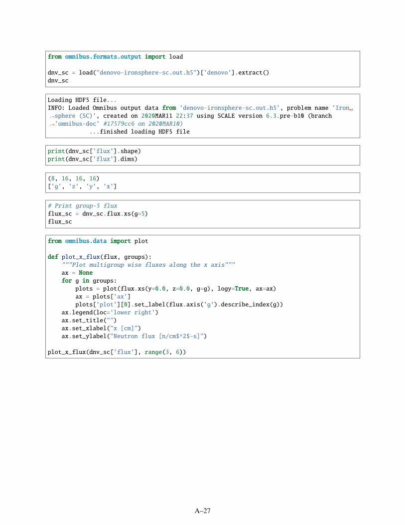
from omnibus.formats.output import load
dnv_sc = load("denovo-ironsphere-sc.out.h5")['denovo'].extract()dnv_sc
Loading HDF5 file...INFO: Loaded Omnibus output data from 'denovo-ironsphere-sc.out.h5', problem name 'Iron→sphere (SC)', created on 2020MAR11 22:37 using SCALE version 6.3.pre-b10 (branch→'omnibus-doc' #17579cc6 on 2020MAR10)
...finished loading HDF5 file
print(dnv_sc['flux'].shape)print(dnv_sc['flux'].dims)
(8, 16, 16, 16)['g', 'z', 'y', 'x']
# Print group-5 fluxflux_sc = dnv_sc.flux.xs(g=5)flux_sc
from omnibus.data import plot
def plot_x_flux(flux, groups):"""Plot multigroup wise fluxes along the x axis"""ax = Nonefor g in groups:
plots = plot(flux.xs(y=0.0, z=0.0, g=g), logy=True, ax=ax)ax = plots['ax']plots['plot'][0].set_label(flux.axis('g').describe_index(g))
ax.legend(loc='lower right')ax.set_title("")ax.set_xlabel("x [cm]")ax.set_ylabel("Neutron flux [n/cm$^2$-s]")
plot_x_flux(dnv_sc['flux'], range(3, 6))
A–27

Two-dimensional pseudocolor plots of the flux are easy to render. Note that the ray effects seen in thefollowing plot are characteristic of any discrete ordinate method, including SC.
flux_slice = dnv_sc['flux'].xs(g=5, y=0.0)print("Flux spans :.2e to :.2e".format(
flux_slice.data.min(),flux_slice.data.max()))
Flux spans 3.72e-06 to 3.88e-03
from matplotlib.colors import Normalize, LogNorm
def plot_pcolor(flux):norm = LogNorm(vmin=1e-8, vmax=1e-2)plots = plot(flux.xs(g=3, y=0.0), norm=norm)plots['ax'].title.set_position([.5, 1.05])plots = plot(flux.xs(g=3, x=5.0), norm=norm)plots['ax'].title.set_position([.5, 1.05])
plot_pcolor(dnv_sc['flux'])
A–28

A.2.2.3 LD results
The following changes to the base input run Omnibus with LD instead of SC.
A–29

%cat SOURCE_DIR/data/denovo-ironsphere.ld.py
cat: /rnsdhpc/code/src/scale/Exnihilo/packages/Omnibus/driver/example/data/denovo-→ironsphere.ld.py: No such file or directory
!omnibus-run SOURCE_DIR/data/denovo-ironsphere.omn SOURCE_DIR/data/denovo-ironsphere-→ld.py
INFO: Starting Omnibus preprocessor, omnibus version 6.3.pre-b10 (branch 'omnibus-doc'→#98d73c8e on 2020MAR11)Loading problem db from Omnibus ASCII file...Loading Omnibus input file at /rnsdhpc/code/src/scale/Exnihilo/packages/Omnibus/driver/→example/data/denovo-ironsphere.omn
...finished loading problem db from Omnibus ASCII fileLoading problem db from Python file...
...finished loading problem db from Python fileLoading problem db from Python file...
...finished loading problem db from Python fileINFO: Set default for 'mpiexec_args' to '['-np', '4']' in '/run'Generating MCNP runtpe file...
...finished generating MCNP runtpe file>>> Loading nuclide data from processed MCNP libraries>>> Loading compositions from MCNP input>>> Loading nuclide data from processed MCNP libraries>>> Loading compositions from MCNP inputINFO: Set default for 'disable_upscattering' to 'False' in '/physics/mg'INFO: Set default for 'load_scl' to 'True' in '/comp'INFO: Set default for 'physics' to 'mg' in '/denovo'WARNING: The 'method' keyword is now 'equations' for SN discretization types. Changing→`method ld` to `equations ld`INFO: Set default for 'boundary' to ''_type': 'vacuum'' in '/denovo'INFO: Set default 'x_blocks 2' and 'y_blocks 2'INFO: Set default for 'z_blocks' to '2' in '/denovo/decomposition'INFO: Set default for 'mat' to 'True' in '/denovo/output'INFO: Set default for 'source' to 'True' in '/denovo/output'INFO: Set default for 'flux' to 'True' in '/denovo/output'INFO: Set default for 'upscatter_groups' to 'thermal' in '/denovo/solver'INFO: Method: snINFO: Equations: ldINFO: Set default for 'solver' to 'gmres' in '/denovo/solver/upscatter'INFO: Method: snINFO: Equations: ldINFO: Set default for 'tolerance' to '0.001' in '/denovo/solver/upscatter'INFO: Set default for 'preconditioner' to ''_type': 'none'' in '/denovo/solver/→upscatter'INFO: Set default for 'max_iterations' to '1000' in '/denovo/solver/upscatter'INFO: Set default for 'verbosity' to 'low' in '/denovo/solver/upscatter'INFO: Method: snINFO: Equations: ldINFO: Set default for 'solver' to 'gmres' in '/denovo/solver/within_group'INFO: Method: sn
(continues on next page)
A–30

(continued from previous page)
INFO: Equations: ldINFO: Set default for 'tolerance' to '0.001' in '/denovo/solver/within_group'INFO: Set default for 'preconditioner' to ''_type': 'none'' in '/denovo/solver/within_→group'INFO: Global Denovo mesh has 4096 cellsINFO: Renaming existing file denovo-ironsphere.inp.xml to denovo-ironsphere.inp-20200311-→2237a.xmlINFO: Writing Omnibus input ParameterList to denovo-ironsphere.inp.xml>>> Loading SCALE Standard Composition Library from /usr/local/scale/data/scale.rev40.→sclibGenerating geometry image...INFO: Saved geometry image at z=0 to 'plot000_z0.pdf'
...finished generating geometry imageINFO: Renaming existing file denovo-ironsphere.pp.json to denovo-ironsphere.pp-20200311-→2237a.jsonINFO: Writing preprocessed file to denovo-ironsphere.pp.jsonINFO: Renaming existing file denovo-ironsphere.inp.omn to denovo-ironsphere.inp-20200311-→2237.omnINFO: Writing processed ASCII input to 'denovo-ironsphere.inp.omn'INFO: Launching Omnibus driver on 4 coresRunning Omnibus...INFO: Renaming existing file omnibus.out to omnibus-20200311-2237.outINFO: Renaming existing file omnibus.err to omnibus-20200311-2237.errWARNING: The Exnihilo software revision (r540) used to generate the input file differs→from this version being used to run it (r539).WARNING: This could cause internal consistency checks to unexpectedly fail, and it could→even lead to unexpected database value changes.WARNING: Please check your output very carefully after this run to make sure the→interpreted values match your input values.Building modelINFO: Loading SCALE Standard Composition Library from /usr/local/scale/data/scale.rev40.→sclibINFO: Loading compositions from MCNP inputWARNING: Extents of MCNP geometry are extremely large or unknown; this may adversely→affect 'global' tallies, entropy mesh, etc.Building physics 'mg'INFO: Loading AMPX library at '/usr/local/scale/data/test8g_v7.1'INFO: Retained 21 of 449 nuclides on the master AMPX libraryINFO: Running XSProc on 2 cellsWARNING: Remapped 2 nuclide IDs: 6012->6000, 6013->6000Building sourcesBuilding Denovo solver internalsRay tracing Denovo meshMixing Denovo cross sectionsBuilding Denovo sourcesConstructing forward sources for DenovoWARNING: MCNP source discretization is currently experimental: only a single isotropic→volumetric source will be treated correctly.WARNING: Discretization of source (type MCNP) was undersampled (undersampling fraction 0.→999329).WARNING: Consider increasing the number of samples per batch or decreasing the source→bounding box to (-0.952794,-0.952794,-0.952794) - (0.952794,0.952794,0.952794)
(continues on next page)
A–31

(continued from previous page)
Initializing Denovo solverINFO: Constructing Denovo state vector with 8 groups, 4096 cells, 16 moments, 4 unknowns→per cellRunning Denovo transport calculationForward group 0 finished in 3 Belos Block GMRES iterations in 1 s...Forward group 1 finished in 4 Belos Block GMRES iterations in 1 s...Forward group 2 finished in 5 Belos Block GMRES iterations in 1 s...Forward group 3 finished in 4 Belos Block GMRES iterations in 1 s...INFO: Forward groups 4-7 finished in 37 Belos Block GMRES iterations.INFO: Writing Silo file to 4 concurrent files using material volume fractionsINFO: Removing SILO directory denovo_output_siloWriting Denovo HDF5 outputRun completeCleaning upBelos Block GMRES converged after 37 iterations.>>> Forward groups 4-7 finished in 37 Belos Block GMRES iterations.
...finished running Omnibus in 6.1 secondsRunning Omnibus postprocessingLoading HDF5 file...INFO: Loaded Omnibus output data from 'denovo-ironsphere-ld.out.h5', problem name 'Iron→sphere (LD)', created on 2020MAR11 22:37 using SCALE version 6.3.pre-b10 (branch→'omnibus-doc' #17579cc6 on 2020MAR10)
...finished loading HDF5 fileLoading HDF5 file...INFO: Loaded Omnibus output data from 'denovo-ironsphere-ld.out.h5', problem name 'Iron→sphere (LD)', created on 2020MAR11 22:37 using SCALE version 6.3.pre-b10 (branch→'omnibus-doc' #17579cc6 on 2020MAR10)
...finished loading HDF5 fileWriting Denovo visualization file...INFO: Wrote Denovo visualization file to denovo-ironsphere-ld.denovo.xmf
...finished writing Denovo visualization fileBuilding RST summary...INFO: Wrote summary file to denovo-ironsphere-ld.rst
...finished building RST summary
dnv_ld = load("denovo-ironsphere-ld.out.h5")['denovo'].extract()plot_x_flux(dnv_ld['flux'], range(3, 6))plot_pcolor(dnv_ld['flux'])
Loading HDF5 file...INFO: Loaded Omnibus output data from 'denovo-ironsphere-ld.out.h5', problem name 'Iron→sphere (LD)', created on 2020MAR11 22:37 using SCALE version 6.3.pre-b10 (branch→'omnibus-doc' #17579cc6 on 2020MAR10)
...finished loading HDF5 file
A–32

A–33

Again, notice the ray effects in the scalar flux plot below due to LD being a discrete ordinates method.
A.2.2.4 Run with SPN
A final set of changes to the base input runs Omnibus with SP3.
%cat SOURCE_DIR/data/denovo-ironsphere-spn.py
################################################################################ File : Omnibus/driver/example/data/denovo-ironsphere-spn.py# Date : Fri Nov 18 14:03:23 2016################################################################################from __future__ import (division, absolute_import, print_function, )#-----------------------------------------------------------------------------#
# Modify the problem namedb['problem']['name'] += " (SPN)"db['output'] = 'output': 'denovo-ironsphere-spn.out.h5'
# Set the method to 'spn'db['denovo']['method'] = "spn"# Delete the inapplicable databasesdel db['denovo']['quadrature']del db['denovo']['solver']['within_group']
################################################################################ end of Omnibus/driver/example/data/denovo-ironsphere-spn.py###############################################################################
A–34

!omnibus-run SOURCE_DIR/data/denovo-ironsphere.omn SOURCE_DIR/data/denovo-ironsphere-→spn.py
INFO: Starting Omnibus preprocessor, omnibus version 6.3.pre-b10 (branch 'omnibus-doc'→#98d73c8e on 2020MAR11)Loading problem db from Omnibus ASCII file...Loading Omnibus input file at /rnsdhpc/code/src/scale/Exnihilo/packages/Omnibus/driver/→example/data/denovo-ironsphere.omn
...finished loading problem db from Omnibus ASCII fileLoading problem db from Python file...
...finished loading problem db from Python fileLoading problem db from Python file...
...finished loading problem db from Python fileINFO: Set default for 'mpiexec_args' to '['-np', '4']' in '/run'Generating MCNP runtpe file...
...finished generating MCNP runtpe file>>> Loading nuclide data from processed MCNP libraries>>> Loading compositions from MCNP input>>> Loading nuclide data from processed MCNP libraries>>> Loading compositions from MCNP inputINFO: Set default for 'disable_upscattering' to 'False' in '/physics/mg'INFO: Set default for 'load_scl' to 'True' in '/comp'INFO: Set default for 'physics' to 'mg' in '/denovo'INFO: Set default for 'boundary' to ''_type': 'vacuum'' in '/denovo'INFO: Set default 'x_blocks 2' and 'y_blocks 2'INFO: Set default for 'mat' to 'True' in '/denovo/output'INFO: Set default for 'source' to 'True' in '/denovo/output'INFO: Set default for 'flux' to 'True' in '/denovo/output'INFO: Set default for 'upscatter_groups' to 'all' in '/denovo/solver'INFO: Method: spnINFO: Set default for 'solver' to 'gmres' in '/denovo/solver/upscatter'INFO: Method: spnINFO: Set default for 'tolerance' to '0.001' in '/denovo/solver/upscatter'INFO: Set default for 'preconditioner' to ''_type': 'none'' in '/denovo/solver/→upscatter'INFO: Set default for 'max_iterations' to '1000' in '/denovo/solver/upscatter'INFO: Set default for 'verbosity' to 'low' in '/denovo/solver/upscatter'INFO: Global Denovo mesh has 4096 cellsINFO: Renaming existing file denovo-ironsphere.inp.xml to denovo-ironsphere.inp-20200311-→2237b.xmlINFO: Writing Omnibus input ParameterList to denovo-ironsphere.inp.xml>>> Loading SCALE Standard Composition Library from /usr/local/scale/data/scale.rev40.→sclibGenerating geometry image...INFO: Saved geometry image at z=0 to 'plot000_z0.pdf'
...finished generating geometry imageINFO: Renaming existing file denovo-ironsphere.pp.json to denovo-ironsphere.pp-20200311-→2237b.jsonINFO: Writing preprocessed file to denovo-ironsphere.pp.jsonINFO: Renaming existing file denovo-ironsphere.inp.omn to denovo-ironsphere.inp-20200311-→2237a.omnINFO: Writing processed ASCII input to 'denovo-ironsphere.inp.omn'
(continues on next page)
A–35

(continued from previous page)
INFO: Launching Omnibus driver on 4 coresRunning Omnibus...INFO: Renaming existing file omnibus.out to omnibus-20200311-2237a.outINFO: Renaming existing file omnibus.err to omnibus-20200311-2237a.errWARNING: The Exnihilo software revision (r540) used to generate the input file differs→from this version being used to run it (r539).WARNING: This could cause internal consistency checks to unexpectedly fail, and it could→even lead to unexpected database value changes.WARNING: Please check your output very carefully after this run to make sure the→interpreted values match your input values.Building modelINFO: Loading SCALE Standard Composition Library from /usr/local/scale/data/scale.rev40.→sclibINFO: Loading compositions from MCNP inputWARNING: Extents of MCNP geometry are extremely large or unknown; this may adversely→affect 'global' tallies, entropy mesh, etc.Building physics 'mg'INFO: Loading AMPX library at '/usr/local/scale/data/test8g_v7.1'INFO: Retained 21 of 449 nuclides on the master AMPX libraryINFO: Running XSProc on 2 cellsWARNING: Remapped 2 nuclide IDs: 6012->6000, 6013->6000Building sourcesBuilding Denovo solver internalsRay tracing Denovo meshMixing Denovo cross sectionsBuilding Denovo sourcesConstructing forward sources for DenovoWARNING: MCNP source discretization is currently experimental: only a single isotropic→volumetric source will be treated correctly.WARNING: Discretization of source (type MCNP) was undersampled (undersampling fraction 0.→999329).WARNING: Consider increasing the number of samples per batch or decreasing the source→bounding box to (-0.952794,-0.952794,-0.952794) - (0.952794,0.952794,0.952794)Initializing Denovo solverINFO: Built SPN FV Element LHS Matrix with 1333248 nonzero entries.Running Denovo transport calculationINFO: Writing Silo file to 4 concurrent files using material volume fractionsINFO: Removing SILO directory denovo_output_siloWriting Denovo HDF5 outputRun completeCleaning upBelos Block GMRES converged after 274 iterations.
...finished running Omnibus in 2.1 secondsRunning Omnibus postprocessingLoading HDF5 file...INFO: Loaded Omnibus output data from 'denovo-ironsphere-spn.out.h5', problem name 'Iron→sphere (SPN)', created on 2020MAR11 22:37 using SCALE version 6.3.pre-b10 (branch→'omnibus-doc' #17579cc6 on 2020MAR10)
...finished loading HDF5 fileLoading HDF5 file...INFO: Loaded Omnibus output data from 'denovo-ironsphere-spn.out.h5', problem name 'Iron→sphere (SPN)', created on 2020MAR11 22:37 using SCALE version 6.3.pre-b10 (branch→'omnibus-doc' #17579cc6 on 2020MAR10) (continues on next page)
A–36

(continued from previous page)
...finished loading HDF5 fileWriting Denovo visualization file...INFO: Wrote Denovo visualization file to denovo-ironsphere-spn.denovo.xmf
...finished writing Denovo visualization fileBuilding RST summary...INFO: Wrote summary file to denovo-ironsphere-spn.rst
...finished building RST summary
dnv_spn = load("denovo-ironsphere-spn.out.h5")['denovo'].extract()plot_x_flux(dnv_spn['flux'], range(3, 6))plot_pcolor(dnv_spn['flux'])
Loading HDF5 file...INFO: Loaded Omnibus output data from 'denovo-ironsphere-spn.out.h5', problem name 'Iron→sphere (SPN)', created on 2020MAR11 22:37 using SCALE version 6.3.pre-b10 (branch→'omnibus-doc' #17579cc6 on 2020MAR10)
...finished loading HDF5 file
A–37

Note that the SPN method demonstrates no ray effects since it is a spherical harmonics method rather than adiscrete ordinates method.
A–38

A.2.2.5 Compare the three methods
A final plot summarizes results from the three spatial discretization methods, plotting along the x axis (wherey = 0 and z = 0).
The SP3 solution is depressed at the source material bounary as expected.
All solutions agree well farther from the source.
labeled_data = [('SC', dnv_sc),('LD', dnv_ld),('SPN', dnv_spn)]
ax = Nonefor (label, data) in labeled_data:
plots = plot(data.flux.xs(y=0.0, z=0.0, g=3), logy=True, ax=ax)plots['plot'][0].set_label(label)ax = plots['ax']
ax.set_xlabel("x [cm]")ax.set_ylabel("Neutron flux [n/cm$^2$-s]")ax.set_title("Neutron flux : energy group 3")ax.legend();
A.2.3 KOBAYASHI PROBLEM 1.II
This example compares Denovo results to published transport benchmark results [1].
# Set up example environmentimport osfrom exnihilotools.matplotlib import screen_style
(continues on next page)
A–39

(continued from previous page)
%matplotlib inlinescreen_style()SOURCE_DIR = os.environ.get("SOURCE_DIR", ".")
A.2.3.1 Visualizing geometry
The geometry is loaded from the GG input file to create a raytrace imager for visualizing the geometry. Thefrom_extents method works for geometries that have bounding boxes (e.g., GG, SCALE, SWORD)..
from geometria import GG_Geometryfrom omnibus.raytrace.imager import Imagerfrom omnibus.raytrace.load import load_gg
model = load_gg(os.path.join(SOURCE_DIR, "data", "kobp1.gg.omn"))imager = Imager.from_extents(model.geometry, x=0, trace='cell')imager.plot();
Generating Geometria XML input file from .gg.omn...INFO: Starting Geometria preprocessor, omnibus version 6.3.pre-b10 (branch 'omnibus-doc'→#98d73c8e on 2020MAR11)Loading problem db from Omnibus ASCII file...Loading Omnibus input file at /rnsdhpc/code/src/scale/Exnihilo/packages/Omnibus/driver/→example/data/kobp1.gg.omn
...finished loading problem db from Omnibus ASCII fileINFO: Writing Geometria input ParameterList to kobp1.gg.xml
...finished generating Geometria XML input file from .gg.omn
A–40

A.2.3.2 Kobayashi Cross Sections
Now the Exnihilo python wrappers are used to generate analytic 1-group cross sections for the Kobayashiproblem. The Materials class is a simple working multigroup cross section library container.
import robusimport numpy as npfrom nemesis import make_const_viewfrom transcore import XML_Writer
# Create XS containermats = robus.Materials()mats.set_num_materials(4)
# Define names and valuesnum_groups = 1pn_order = 0reactions = [robus.TOTAL, robus.SCATTERING]totals = [0.0, 0.1, 1.0e-5, 0.1]names = ['vaccum', 'region 1', 'region 2', 'region 3']c = 0.5
# Construct cross sectionsfor (i, tot_xs) in enumerate(totals):
mat = robus.Material_Downscatter(reactions, num_groups, pn_order)total = np.array([tot_xs])mat.set_sigma(make_const_view(total))scat = np.array([[[c * tot_xs]]])mat.set_sigma_s(make_const_view(scat))mat.complete()mats.set_material(i, mat)
mats.complete()
# Write to XS input filewriter = XML_Writer(mats, "kobayashi_ii.xs.xml", names)writer.write()
A.2.3.3 Execute Omnibus
Because the cross sections we generated are in the working directory, the Omnibus input files must also becopied the working directory too, since paths in the input file are relative to the input file.
%cp SOURCE_DIR/data/denovo-kobayashi.omn .%cp SOURCE_DIR/data/kobp1.gg.omn .%cat denovo-kobayashi.omn
[PROBLEM]name "Kobayashi Problem 1-ii"mode forward
[MODEL=gg]input "kobp1.gg.omn"
(continues on next page)
A–41

(continued from previous page)
[PHYSICS=mg]pn_order 0num_groups 1neutron_bounds 2e7 1e-5 ! arbitraryxml_path "kobayashi_ii.xs.xml"
[SOURCE=separable source]q 1000.0fis False
[SOURCE][SHAPE=box]xmin 0.0xmax 10.0ymin 0.0ymax 10.0zmin 0.0zmax 10.0
[SOURCE][ENERGY=histogram]e 1e-05 2e7p 1.0pt n
[SOURCE][ANGLE=isotropic]
[DENOVO]method scx 0.0 9i 100.0y 0.0 9i 100.0z 0.0 9i 100.0
[DENOVO][BOUNDARY=reflect]reflect 1 0 1 0 1 0
[DENOVO][SOLVER=fixed]tolerance 1e-03[.][WITHIN_GROUP]verbosity none
[DENOVO][QUADRATURE]quadrature glproductconstruction productnum_azi 2num_polar 2
[RUN=mpi]np 4
!omnibus-run denovo-kobayashi.omn
A–42

INFO: Starting Omnibus preprocessor, omnibus version 6.3.pre-b10 (branch 'omnibus-doc'→#98d73c8e on 2020MAR11)Loading problem db from Omnibus ASCII file...Loading Omnibus input file at denovo-kobayashi.omn
...finished loading problem db from Omnibus ASCII fileLoading problem db from Python file...
...finished loading problem db from Python fileINFO: Set default for 'mpiexec_args' to '['-np', '4']' in '/run'Generating Geometria XML input file from .gg.omn...INFO: Starting Geometria preprocessor, omnibus version 6.3.pre-b10 (branch 'omnibus-doc'→#98d73c8e on 2020MAR11)Loading problem db from Omnibus ASCII file...Loading Omnibus input file at /rnsdhpc/code/build/Exnihilo-examples/Exnihilo/packages/→Omnibus/driver/example/denovo-kobayashi/kobp1.gg.omn
...finished loading problem db from Omnibus ASCII fileINFO: Renaming existing file kobp1.gg.xml to kobp1.gg-20200311-2236.xmlINFO: Writing Geometria input ParameterList to kobp1.gg.xml
...finished generating Geometria XML input file from .gg.omnINFO: Set default for 'mode' to 'n' in '/physics/mg'INFO: Set default for 'disable_upscattering' to 'False' in '/physics/mg'INFO: Set default for 'load_scl' to 'False' in '/comp'INFO: Set default for 'physics' to 'mg' in '/denovo'WARNING: The 'method' keyword is now 'equations' for SN discretization types. Changing→`method sc` to `equations sc`INFO: Set default 'x_blocks 2' and 'y_blocks 2'INFO: Set default for 'z_blocks' to '2' in '/denovo/decomposition'INFO: Set default for 'mat' to 'True' in '/denovo/output'INFO: Set default for 'source' to 'True' in '/denovo/output'INFO: Set default for 'uncflux' to 'True' in '/denovo/output'INFO: Set default for 'flux' to 'True' in '/denovo/output'INFO: Set default for 'upscatter_groups' to 'thermal' in '/denovo/solver'INFO: Method: snINFO: Equations: scINFO: Set default for 'solver' to 'gmres' in '/denovo/solver/upscatter'INFO: Method: snINFO: Equations: scINFO: Set default for 'tolerance' to '0.001' in '/denovo/solver/upscatter'INFO: Set default for 'preconditioner' to ''_type': 'none'' in '/denovo/solver/→upscatter'INFO: Set default for 'max_iterations' to '1000' in '/denovo/solver/upscatter'INFO: Set default for 'verbosity' to 'low' in '/denovo/solver/upscatter'INFO: Method: snINFO: Equations: scINFO: Set default for 'solver' to 'gmres' in '/denovo/solver/within_group'INFO: Method: snINFO: Equations: scINFO: Set default for 'tolerance' to '0.001' in '/denovo/solver/within_group'INFO: Set default for 'preconditioner' to ''_type': 'none'' in '/denovo/solver/within_→group'INFO: Global Denovo mesh has 1000 cellsINFO: Writing Omnibus input ParameterList to denovo-kobayashi.inp.xmlINFO: Writing preprocessed file to denovo-kobayashi.pp.json
(continues on next page)
A–43

(continued from previous page)
INFO: Writing processed ASCII input to 'denovo-kobayashi.inp.omn'INFO: Launching Omnibus driver on 4 coresRunning Omnibus...WARNING: The Exnihilo software revision (r540) used to generate the input file differs→from this version being used to run it (r539).WARNING: This could cause internal consistency checks to unexpectedly fail, and it could→even lead to unexpected database value changes.WARNING: Please check your output very carefully after this run to make sure the→interpreted values match your input values.Building modelINFO: No composition data is present in the GG model at '/rnsdhpc/code/build/Exnihilo-→examples/Exnihilo/packages/Omnibus/driver/example/denovo-kobayashi/kobp1.gg.xml'INFO: Creating default boundary mesh from (0 0 0) to (100 100 100) for GG geometryBuilding physics 'mg'Building sourcesBuilding Denovo solver internalsRay tracing Denovo meshMixing Denovo cross sectionsBuilding Denovo sourcesConstructing forward sources for DenovoInitializing Denovo solverINFO: Constructing Denovo state vector with 1 groups, 1000 cells, 1 moments, 1 unknowns→per cellRunning Denovo transport calculationINFO: Writing Silo file to 4 concurrent files using material volume fractionsWriting Denovo HDF5 outputRun completeCleaning upForward group 0 finished in 6 Belos Block GMRES iterations in 1 s...
...finished running Omnibus in 1.2 secondsRunning Omnibus postprocessingLoading HDF5 file...INFO: Loaded Omnibus output data from 'denovo-kobayashi.out.h5', problem name 'Kobayashi→Problem 1-ii', created on 2020MAR11 22:36 using SCALE version 6.3.pre-b10 (branch→'omnibus-doc' #17579cc6 on 2020MAR10)
...finished loading HDF5 fileLoading HDF5 file...INFO: Loaded Omnibus output data from 'denovo-kobayashi.out.h5', problem name 'Kobayashi→Problem 1-ii', created on 2020MAR11 22:36 using SCALE version 6.3.pre-b10 (branch→'omnibus-doc' #17579cc6 on 2020MAR10)
...finished loading HDF5 fileWriting Denovo visualization file...INFO: Wrote Denovo visualization file to denovo-kobayashi.denovo.xmf
...finished writing Denovo visualization fileBuilding RST summary...INFO: Wrote summary file to denovo-kobayashi.rst
...finished building RST summary
The run generates several files, including an HDF5 file with the denovo solution data and a ReStructured Textfile that summarizes the problem run.
A–44

assert os.path.exists("denovo-kobayashi.out.h5")
A.2.3.4 Check the source term
Verifying the computational input is an important step in analysis. Plotting the source region (again only ingroup zero) reveals that it has a single nonzero source mesh cell.
Since this is a one-group problem, it is easier to extract group zero at the beginning. Clearing the hyperslicefield reduces clutter by discarding the metadata that this source object is group zero.
from omnibus.formats.output import load
dnv = load("denovo-kobayashi.out.h5")['denovo'].extract()
source = dnv.source.xs(g=0)source.hyperslice = []source
Loading HDF5 file...INFO: Loaded Omnibus output data from 'denovo-kobayashi.out.h5', problem name 'Kobayashi→Problem 1-ii', created on 2020MAR11 22:36 using SCALE version 6.3.pre-b10 (branch→'omnibus-doc' #17579cc6 on 2020MAR10)
...finished loading HDF5 file
from omnibus.data import plot
print(np.count_nonzero(source))plot(source.xs(x=5.0));
1
A–45

A.2.3.5 Visualize the flux
flux = dnv.flux.xs(g=0)flux.hyperslice = []flux
This code plots a lineout along the z axis in the cell where x = y = 5:
plots = plot(flux.xs(x=5, y=5), logy=True)ax = plots['ax']ax.set_title(ax.get_ylabel())ax.set_ylabel("Particle flux (p/cm^2-s)");
A–46

A pseudocolor plot can visualize the flux. The options on the matplotlib LogNorm class constrain the rangeof the color scale.
from matplotlib.colors import LogNorm
norm = LogNorm(vmin=1e-6, vmax=1)plot(flux.xs(z=5.0), norm=norm);plot(flux.xs(x=5.0), norm=norm);
A–47

Compare against reference solutions
The reference data in the Kobayashi paper are point samples formatted as (x, y, z, φ). They comprise threelineouts: one along y, one along x = y = z, and one along x.
A–48

from six.moves import StringIOimport numpy as np
# X, Y, Z, referenceref_y = """5 5 5 8.29260E+005 15 5 1.87028E+005 25 5 7.13986E-015 35 5 3.84685E-015 45 5 2.53984E-015 55 5 1.37220E-015 65 5 4.65913E-025 75 5 1.58766E-025 85 5 5.47036E-035 95 5 1.85082E-03"""ref_xyz = """5 5 5 8.29260E+0015 15 15 6.63233E-0125 25 25 2.68828E-0135 35 35 1.56683E-0145 45 45 1.04405E-0155 55 55 3.02145E-0265 65 65 4.06555E-0375 75 75 5.86124E-0485 85 85 8.66059E-0595 95 95 1.12892E-05"""ref_x = """5 55 5 1.37220E-0115 55 5 1.27890E-0125 55 5 1.13582E-0135 55 5 9.59578E-0245 55 5 7.82701E-0255 55 5 5.67030E-0265 55 5 1.88631E-0275 55 5 6.46624E-0385 55 5 2.28099E-0395 55 5 7.93924E-04"""ref_y = np.loadtxt(StringIO(ref_y))ref_xyz = np.loadtxt(StringIO(ref_xyz))ref_x = np.loadtxt(StringIO(ref_x))
Since these are all physical points, it is easy to use the meshes to look up the points where the reference datais using the xs method.
import matplotlib.pyplot as plt
# Get a line-out of the actual fluxx_phi = flux.xs(y=55, z=5)# Extract calculated points along the coordinate mesh
(continues on next page)
A–49

(continued from previous page)
x_mesh = ref_x[:,0]act = np.array([x_phi.xs(x=x).data for x in x_mesh])# Get the reference valuesref = ref_x[:,3]
(fig, (flux_ax, ratio_ax)) = plt.subplots(2, 1, figsize=(4, 4), sharex=True)# Plot the actual lineoutplot(x_phi, ax=flux_ax)# Plot the ratiosratio_ax.plot(x_mesh, act/ref - 1)
flux_ax.set_ylabel(r'$\phi$')ratio_ax.set_xlabel("$x$ (cm)")ratio_ax.set_ylabel(r"$\phi / \phi_\mathrmref - 1$");
axis = ref_y[:,1]y_phi = flux.xs(x=5, z=5)act = np.array([y_phi.xs(y=y).data for y in axis])ref = ref_y[:,3]
(fig, ax) = plt.subplots()ax.plot(axis, act/ref - 1)ax.set_xlabel("$y$ (cm)")ax.set_ylabel("$\phi / \phi_\mathrmref - 1$");
A–50
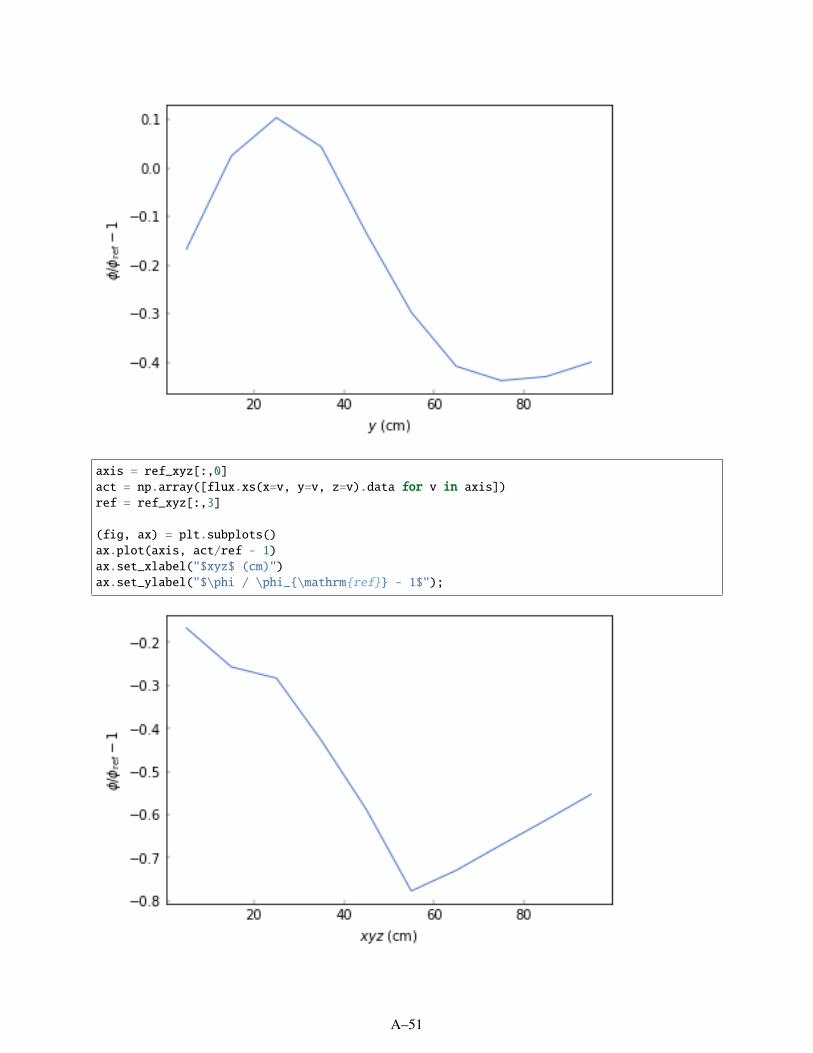
axis = ref_xyz[:,0]act = np.array([flux.xs(x=v, y=v, z=v).data for v in axis])ref = ref_xyz[:,3]
(fig, ax) = plt.subplots()ax.plot(axis, act/ref - 1)ax.set_xlabel("$xyz$ (cm)")ax.set_ylabel("$\phi / \phi_\mathrmref - 1$");
A–51

A.2.4 UEKI BENCHMARK PROBLEM
This example uses Denovo to determine a dose rate to the detector, and it demonstrates using the adjointsolution capability to obtain an importance function. Since this problem also contains a point source, it showshow an “uncollided flux” treatment can reduce ray effects. Two approximation methods for the uncollidedflux source (uncf) will be explored: the “analytic” approximation, where the source is physically raytraced toevery computational cell in the geometry; and a Monte Carlo approximation, where numerous samples froma stochastic point source generate the deterministic source term.
# Set up example environmentimport osSOURCE_DIR = os.environ.get("SOURCE_DIR", ".")%matplotlib inlinefrom exnihilotools.matplotlib import screen_stylescreen_style()
A.2.4.1 Pre-visualize the geometry
The [PLOT][PRE] block in the input file generates a 2D image of the problem geometry for visualizingbefore actually executing the problem.
The Ueki problem consists of a neutron source is placed at the center of a block of paraffin with a 45 degreecone-shaped opening at the front. This opening points toward a graphite shield of varying thickness, with anideal detector on the far side.
!grep -A 5 "\[PRE\]" SOURCE_DIR/data/denovo-ueki-adj.omn!omnibus-pre SOURCE_DIR/data/denovo-ueki-adj.omn
[PRE][PRE][PLOT lateral]origin -25 0 -40size 127.5 80axis yrender trueINFO: Starting Omnibus preprocessor, omnibus version 6.3.pre-b10 (branch 'omnibus-doc'→#98d73c8e on 2020MAR11)Loading problem db from Omnibus ASCII file...Loading Omnibus input file at /rnsdhpc/code/src/scale/Exnihilo/packages/Omnibus/driver/→example/data/denovo-ueki-adj.omn
...finished loading problem db from Omnibus ASCII fileLoading problem db from Python file...
...finished loading problem db from Python fileINFO: Set default for 'mpiexec_args' to '['-np', '4']' in '/run'Generating MCNP runtpe file...MCNP: xact is done ...finished generating MCNP runtpe file>>> Loading nuclide data from processed MCNP libraries>>> Loading compositions from MCNP input>>> Loading nuclide data from processed MCNP libraries>>> Loading compositions from MCNP inputINFO: Set default for 'load_scl' to 'True' in '/comp'INFO: Set default for 'physics' to 'mg' in '/denovo'WARNING: The 'method' keyword is now 'equations' for SN discretization types. Changing→`method sc` to `equations sc`
(continues on next page)
A–52

(continued from previous page)
INFO: Set default for 'boundary' to ''_type': 'vacuum'' in '/denovo'INFO: Set default 'x_blocks 2' and 'y_blocks 2'INFO: Set default for 'z_blocks' to '2' in '/denovo/decomposition'INFO: Set default for 'quadrature' to 'qr' in '/denovo/quadrature'INFO: Set default for 'construction' to 'product' in '/denovo/quadrature'INFO: Set default for 'mat' to 'True' in '/denovo/output'INFO: Set default for 'source' to 'True' in '/denovo/output'INFO: Set default for 'uncflux' to 'True' in '/denovo/output'INFO: Set default for 'flux' to 'True' in '/denovo/output'INFO: Set default for 'upscatter_groups' to 'thermal' in '/denovo/solver'INFO: Method: snINFO: Equations: scINFO: Set default for 'solver' to 'gmres' in '/denovo/solver/within_group'INFO: Method: snINFO: Equations: scINFO: Set default for 'tolerance' to '0.001' in '/denovo/solver/within_group'INFO: Set default for 'preconditioner' to ''_type': 'none'' in '/denovo/solver/within_→group'INFO: Global Denovo mesh has 4950 cellsINFO: Writing Omnibus input ParameterList to denovo-ueki-adj.inp.xml>>> Loading SCALE Standard Composition Library from /usr/local/scale/data/scale.rev40.→sclibGenerating geometry image...INFO: Saved geometry image at y=0 to 'lateral_y0.png'
...finished generating geometry imageINFO: Writing preprocessed file to denovo-ueki-adj.pp.json
from IPython.display import display, Imagedisplay(Image(filename="lateral_y0.png"))
A–53

A.2.4.2 Analytic uncollided flux results
The uncollided flux from a point source is the solution to a purely absorbing transport equation in each group:
Ω · ∇ψg + σgψg =qg
4πδ(r − r0).
This equation has a simple Green’s function solution:
ψg = δ(Ω −Ω0→r)qg
4π|r − r0|2e−τ(r0,r).
Denovo calculates the total optical thickness τ between the point source and every point on the grid cell, andusing the source spectrum, constructs an analytic solution to the first-collision source. The uncf analyticoption in the [DENOVO][SOURCE] block enables this feature.
%cat SOURCE_DIR/data/denovo-ueki-fwd-uncf-analytic.omn
[PROBLEM]name "Ueki 30cm benchmark (analytic forward source)"mode forward
[MODEL=mcnp]input "../data/ueki.mcnp"
[SOURCE=separable cf252]strength 4.05e7 ! neutrons/sec
(continues on next page)
A–54

(continued from previous page)
[SOURCE][SHAPE=point]point 0.001 0 0
[SOURCE][ENERGY=watt]a 1.025b 2.926
[SOURCE][ANGLE=isotropic]
[PHYSICS=mg]mg_lib "v7-28n19g"pn_order 1disable_upscattering true
[DENOVO]method scx -25 5i 0 5i 60 5i 90 3i 112.5y -40 2i -25 2i -2.5 2i 2.5 2i 25 2i 40z -40 2i -25 2i -2.5 2i 2.5 2i 25 2i 40
[DENOVO][SOLVER=fixed][.][WITHIN_GROUP]verbosity none
[DENOVO][SOURCE]uncf analytic
[DENOVO][QUADRATURE]num_azi 2num_polar 2
[RUN=mpi]np 4
!omnibus-run SOURCE_DIR/data/denovo-ueki-fwd-uncf-analytic.omn
INFO: Starting Omnibus preprocessor, omnibus version 6.3.pre-b10 (branch 'omnibus-doc'→#98d73c8e on 2020MAR11)Loading problem db from Omnibus ASCII file...Loading Omnibus input file at /rnsdhpc/code/src/scale/Exnihilo/packages/Omnibus/driver/→example/data/denovo-ueki-fwd-uncf-analytic.omn
...finished loading problem db from Omnibus ASCII fileLoading problem db from Python file...
...finished loading problem db from Python fileINFO: Set default for 'mpiexec_args' to '['-np', '4']' in '/run'Generating MCNP runtpe file...
...finished generating MCNP runtpe fileINFO: Set default for 'fissionable_only' to 'False' in '/source/cf252'INFO: Set default for 'mode' to 'n' in '/physics/mg'INFO: Set default for 'load_scl' to 'True' in '/comp'INFO: Set default for 'physics' to 'mg' in '/denovo'
(continues on next page)
A–55

(continued from previous page)
WARNING: The 'method' keyword is now 'equations' for SN discretization types. Changing→`method sc` to `equations sc`INFO: Set default for 'boundary' to ''_type': 'vacuum'' in '/denovo'INFO: Set default 'x_blocks 2' and 'y_blocks 2'INFO: Set default for 'z_blocks' to '2' in '/denovo/decomposition'INFO: Set default for 'quadrature' to 'qr' in '/denovo/quadrature'INFO: Set default for 'construction' to 'product' in '/denovo/quadrature'INFO: Set default for 'mat' to 'True' in '/denovo/output'INFO: Set default for 'source' to 'True' in '/denovo/output'INFO: Set default for 'uncflux' to 'True' in '/denovo/output'INFO: Set default for 'flux' to 'True' in '/denovo/output'INFO: Set default for 'upscatter_groups' to 'thermal' in '/denovo/solver'INFO: Method: snINFO: Equations: scINFO: Set default for 'solver' to 'gmres' in '/denovo/solver/within_group'INFO: Method: snINFO: Equations: scINFO: Set default for 'tolerance' to '0.001' in '/denovo/solver/within_group'INFO: Set default for 'preconditioner' to ''_type': 'none'' in '/denovo/solver/within_→group'INFO: Global Denovo mesh has 4950 cellsINFO: Writing Omnibus input ParameterList to denovo-ueki-fwd-uncf-analytic.inp.xmlINFO: Writing preprocessed file to denovo-ueki-fwd-uncf-analytic.pp.jsonINFO: Writing processed ASCII input to 'denovo-ueki-fwd-uncf-analytic.inp.omn'INFO: Launching Omnibus driver on 4 coresRunning Omnibus...WARNING: The Exnihilo software revision (r540) used to generate the input file differs→from this version being used to run it (r539).WARNING: This could cause internal consistency checks to unexpectedly fail, and it could→even lead to unexpected database value changes.WARNING: Please check your output very carefully after this run to make sure the→interpreted values match your input values.Building modelINFO: Loading SCALE Standard Composition Library from /usr/local/scale/data/scale.rev40.→sclibINFO: Loading compositions from MCNP inputINFO: Splitting compound 6000 into at% 6012: 0.9893, 6013: 0.0107INFO: Splitting compound 3006000 into at% 3006012: 0.9893, 3006013: 0.0107WARNING: Extents of MCNP geometry are extremely large or unknown; this may adversely→affect 'global' tallies, entropy mesh, etc.Building physics 'mg'INFO: Loading AMPX library at '/usr/local/scale/data/scale.rev12.xn28g19v7.1'INFO: Retained 3 of 455 nuclides on the master AMPX libraryINFO: Running XSProc on 2 cellsWARNING: Upscattering has been lumped into within-group scattering in the thermal groupsWARNING: Remapped 4 nuclide IDs: 6012->6000, 6013->6000, 3006012->3006000, 3006013->→3006000INFO: Truncating cross sections to groups [0, 28)Building sourcesBuilding Denovo solver internalsRay tracing Denovo meshWARNING: Number of Z blocks (2) is not divisible into the number of z cells 15; reducing→to 1 (continues on next page)
A–56

(continued from previous page)
Mixing Denovo cross sectionsBuilding Denovo sourcesConstructing forward sources for DenovoInitializing Denovo solverINFO: Constructing Denovo state vector with 28 groups, 4950 cells, 4 moments, 1 unknowns→per cellPerforming analytic first-collision source calculation on 1 sourcesRunning Denovo transport calculationForward group 0 finished in 4 Belos Block GMRES iterations.Forward group 1 finished in 4 Belos Block GMRES iterations.Forward group 2 finished in 4 Belos Block GMRES iterations.Forward group 3 finished in 3 Belos Block GMRES iterations.Forward group 4 finished in 4 Belos Block GMRES iterations.Forward group 5 finished in 5 Belos Block GMRES iterations.Forward group 6 finished in 5 Belos Block GMRES iterations.Forward group 7 finished in 6 Belos Block GMRES iterations.Forward group 8 finished in 6 Belos Block GMRES iterations.Forward group 9 finished in 6 Belos Block GMRES iterations.Forward group 10 finished in 6 Belos Block GMRES iterations.Forward group 11 finished in 5 Belos Block GMRES iterations.Forward group 12 finished in 4 Belos Block GMRES iterations.Forward group 13 finished in 4 Belos Block GMRES iterations.Forward group 14 finished in 4 Belos Block GMRES iterations.Forward group 15 finished in 4 Belos Block GMRES iterations.Forward group 16 finished in 3 Belos Block GMRES iterations.Forward group 17 finished in 3 Belos Block GMRES iterations.Forward group 18 finished in 3 Belos Block GMRES iterations.Forward group 19 finished in 3 Belos Block GMRES iterations.Forward group 20 finished in 4 Belos Block GMRES iterations.Forward group 21 finished in 4 Belos Block GMRES iterations.Forward group 22 finished in 4 Belos Block GMRES iterations.Forward group 23 finished in 6 Belos Block GMRES iterations.Forward group 24 finished in 8 Belos Block GMRES iterations.Forward group 25 finished in 9 Belos Block GMRES iterations.Forward group 26 finished in 13 Belos Block GMRES iterations.INFO: Writing Silo file to 4 concurrent files using material volume fractionsWriting Denovo HDF5 outputRun completeCleaning upForward group 27 finished in 39 Belos Block GMRES iterations.
...finished running Omnibus in 3.3 secondsRunning Omnibus postprocessingLoading HDF5 file...INFO: Loaded Omnibus output data from 'denovo-ueki-fwd-uncf-analytic.out.h5', problem→name 'Ueki 30cm benchmark (analytic forward source)', created on 2020MAR11 22:36 using→SCALE version 6.3.pre-b10 (branch 'omnibus-doc' #17579cc6 on 2020MAR10)
...finished loading HDF5 fileLoading HDF5 file...INFO: Loaded Omnibus output data from 'denovo-ueki-fwd-uncf-analytic.out.h5', problem→name 'Ueki 30cm benchmark (analytic forward source)', created on 2020MAR11 22:36 using→SCALE version 6.3.pre-b10 (branch 'omnibus-doc' #17579cc6 on 2020MAR10)
...finished loading HDF5 file(continues on next page)
A–57

(continued from previous page)
Writing Denovo visualization file...INFO: Wrote Denovo visualization file to denovo-ueki-fwd-uncf-analytic.denovo.xmf
...finished writing Denovo visualization fileBuilding RST summary...INFO: Wrote summary file to denovo-ueki-fwd-uncf-analytic.rst
...finished building RST summary
The first-collision method works by splitting the transport equation into uncollided and collided flux compo-nents. The uncollided flux is solved using an analytic approximation. Visualizing the uncollided flux termhelps in verifying the problem setup.
from omnibus.data import plotfrom omnibus.formats.output import load
dnv = load("denovo-ueki-fwd-uncf-analytic.out.h5")['denovo'].extract()uncflux = dnv['uncflux']for g in (2, 5):
plots = plot(uncflux.xs(y=0.0, z=0.0, g=g), logy=True)ax = plots['ax']ax.set_title(ax.get_ylabel())ax.set_ylabel("Uncollided flux (n/cm$^2$-s)")ax.title.set_position([.5, 1.05]);
Loading HDF5 file...INFO: Loaded Omnibus output data from 'denovo-ueki-fwd-uncf-analytic.out.h5', problem→name 'Ueki 30cm benchmark (analytic forward source)', created on 2020MAR11 22:36 using→SCALE version 6.3.pre-b10 (branch 'omnibus-doc' #17579cc6 on 2020MAR10)
...finished loading HDF5 file
A–58

uncf_slice = uncflux.xs(g=2,z=0.0)print("Flux spans :.2e to :.2e".format(
uncf_slice.data.min(),uncf_slice.data.max()))
Flux spans 8.63e-04 to 2.39e+05
Pseudocolor plots show the attenuation of the source term through the material and through space. Since thematerial cross sections depend on energy group, the shape of the uncollided flux terms is different in groups 2and 5.
from matplotlib.colors import LogNorm
norm = LogNorm(vmin=1.0e-5, vmax=1e5)for g in (2, 5):
plots = plot(uncflux.xs(g=g,z=0.0), norm=norm)plots['ax'].title.set_position([.5, 1.25]);
A–59

The flux along the x axis in energy group 2 follows the uncollided flux contribution but also includesinscattering in the material from the higher-energy groups.
plots = plot(dnv['flux'].xs(g=2, y=0, z=0), logy=True)ax = plots['ax']ax.set_title(ax.get_ylabel())ax.set_ylabel("Neutron flux (n/cm$^2$-s)")ax.title.set_position([.5, 1.05]);
A–60

A.2.4.3 Calculate dose rates
The SCALE master library contains American National Standards Institute (ANSI) standard (1977) neutronflux-to-dose conversion factors (rem/hr)/(n/cm^2-s) (MT 9029). The PALEALE code module can be used toprint out these conversion factors from the SCALE AMPX library.
import numpy as np# neutron flux-to-dose conversion factors from ansl/ans 6.1.1 - 1977 02/09/11 (rem/hr)/→(n/cm^2-s)flux_to_dose_factor = np.array([
1.61496E-04, 1.44530E-04, 1.27035E-04, 1.28101E-04, 1.29832E-04, 1.00375E-04,4.53982E-05, 1.19215E-05, 3.72975E-06, 3.71969E-06, 4.00846E-06, 4.29442E-06,4.47304E-06, 4.55834E-06, 4.57702E-06, 4.55983E-06, 4.52102E-06, 4.48745E-06,4.46602E-06, 4.43429E-06, 4.33168E-06, 4.20288E-06, 4.09745E-06, 3.84414E-06,3.66980E-06, 3.67484E-06, 3.67484E-06, 3.67484E-06
])
print("The Denovo output has", len(dnv['flux'].axis('g')), "neutron energy bounds:")print(dnv['flux'].axis('g').bounds.n.tolist())
The Denovo output has 28 neutron energy bounds:[20000000.0, 6376300.0, 3011900.0, 1826800.0, 1422700.0, 907180.0, 407620.0, 111090.0,→15034.0, 3035.39990234375, 582.9500122070312, 101.30000305175781, 29.023000717163086,→10.677000045776367, 5.0, 3.059000015258789, 1.8553999662399292, 1.2999999523162842, 1.→1253000497817993, 1.0, 0.800000011920929, 0.41398999094963074, 0.32499998807907104, 0.→22499999403953552, 0.10000000149011612, 0.05000000074505806, 0.029999999329447746, 0.→009999999776482582, 9.999999747378752e-06]
from omnibus.data import Field
def weighted_energy_integrate(flux, weights, **kwargs):assert len(flux.axis('g')) == len(weights)assert flux.dims[0] == 'g'
(continues on next page)
A–61

(continued from previous page)
axes = flux.axes[1:]result_data = np.zeros([len(ax) for ax in axes])result = Field(axes=axes, data=result_data, **kwargs)
# Perform weighted integralflux_data = flux.datafor g in range(len(flux.axis('g'))):
result_data += weights[g] * flux_data[g]
return result
dose = weighted_energy_integrate(dnv['flux'], flux_to_dose_factor, name='dose', units=→'rem/hr')
The 3D field of doses can be visualized by extracting lineouts or by coloring slices.
plots = plot(dose.xs(y=0, z=0), logy=True)ax = plots['ax']ax.set_ylabel("Dose [rem/hr]")
plots = plot(dose.xs(z=0.0), norm=LogNorm())plots['ax'].title.set_position([.5, 1.25]);
A–62

A.2.4.4 Monte Carlo uncollided flux results
With the Monte Carlo approach, the first collision source (uncollided flux) is obtained by direct Monte Carlosampling. Thus the resulting uncollided flux fluctuates around the mean. As the number of Monte Carloparticles simulated increases, the uncollided flux obtained from the Monte Carlo approach should approachthe analytic uncollided flux. The uncf mc option in the [DENOVO][SOURCE] block enables this feature.
%cat SOURCE_DIR/data/denovo-ueki-fwd-uncf-mc.omn
[PROBLEM]name "Ueki 30cm benchmark (MC forward source)"mode forward
[MODEL=mcnp]input "../data/ueki.mcnp"
[SOURCE=separable cf252]strength 4.05e7 ! neutrons/sec
[SOURCE][SHAPE=point]point 0.001 0 0
[SOURCE][ENERGY=watt]a 1.025b 2.926
[SOURCE][ANGLE=isotropic]
[PHYSICS=mg]mg_lib "v7-28n19g"
(continues on next page)
A–63

(continued from previous page)
pn_order 1disable_upscattering true
[DENOVO]method scx -25 5i 0 5i 60 5i 90 3i 112.5y -40 2i -25 2i -2.5 2i 2.5 2i 25 2i 40z -40 2i -25 2i -2.5 2i 2.5 2i 25 2i 40
[DENOVO][SOLVER=fixed][.][WITHIN_GROUP]verbosity none
[DENOVO][OUTPUT]
[DENOVO][SOURCE]uncf mcmc_num_particles 50000
[DENOVO][QUADRATURE]num_azi 2num_polar 2
[RUN=mpi]np 4
!omnibus-run SOURCE_DIR/data/denovo-ueki-fwd-uncf-mc.omn
INFO: Starting Omnibus preprocessor, omnibus version 6.3.pre-b10 (branch 'omnibus-doc'→#98d73c8e on 2020MAR11)Loading problem db from Omnibus ASCII file...Loading Omnibus input file at /rnsdhpc/code/src/scale/Exnihilo/packages/Omnibus/driver/→example/data/denovo-ueki-fwd-uncf-mc.omn
...finished loading problem db from Omnibus ASCII fileLoading problem db from Python file...
...finished loading problem db from Python fileINFO: Set default for 'mpiexec_args' to '['-np', '4']' in '/run'Generating MCNP runtpe file...
...finished generating MCNP runtpe fileINFO: Set default for 'fissionable_only' to 'False' in '/source/cf252'INFO: Set default for 'mode' to 'n' in '/physics/mg'INFO: Set default for 'load_scl' to 'True' in '/comp'INFO: Set default for 'physics' to 'mg' in '/denovo'WARNING: The 'method' keyword is now 'equations' for SN discretization types. Changing→`method sc` to `equations sc`INFO: Set default for 'boundary' to ''_type': 'vacuum'' in '/denovo'INFO: Set default 'x_blocks 2' and 'y_blocks 2'INFO: Set default for 'z_blocks' to '2' in '/denovo/decomposition'INFO: Set default for 'quadrature' to 'qr' in '/denovo/quadrature'INFO: Set default for 'construction' to 'product' in '/denovo/quadrature'INFO: Set default for 'mat' to 'True' in '/denovo/output'
(continues on next page)
A–64

(continued from previous page)
INFO: Set default for 'source' to 'True' in '/denovo/output'INFO: Set default for 'uncflux' to 'True' in '/denovo/output'INFO: Set default for 'flux' to 'True' in '/denovo/output'INFO: Set default for 'upscatter_groups' to 'thermal' in '/denovo/solver'INFO: Method: snINFO: Equations: scINFO: Set default for 'solver' to 'gmres' in '/denovo/solver/within_group'INFO: Method: snINFO: Equations: scINFO: Set default for 'tolerance' to '0.001' in '/denovo/solver/within_group'INFO: Set default for 'preconditioner' to ''_type': 'none'' in '/denovo/solver/within_→group'INFO: Global Denovo mesh has 4950 cellsINFO: Writing Omnibus input ParameterList to denovo-ueki-fwd-uncf-mc.inp.xmlINFO: Writing preprocessed file to denovo-ueki-fwd-uncf-mc.pp.jsonINFO: Writing processed ASCII input to 'denovo-ueki-fwd-uncf-mc.inp.omn'INFO: Launching Omnibus driver on 4 coresRunning Omnibus...INFO: Renaming existing file omnibus.out to omnibus-20200311-2236.outINFO: Renaming existing file omnibus.err to omnibus-20200311-2236.errWARNING: The Exnihilo software revision (r540) used to generate the input file differs→from this version being used to run it (r539).WARNING: This could cause internal consistency checks to unexpectedly fail, and it could→even lead to unexpected database value changes.WARNING: Please check your output very carefully after this run to make sure the→interpreted values match your input values.Building modelINFO: Loading SCALE Standard Composition Library from /usr/local/scale/data/scale.rev40.→sclibINFO: Loading compositions from MCNP inputINFO: Splitting compound 6000 into at% 6012: 0.9893, 6013: 0.0107INFO: Splitting compound 3006000 into at% 3006012: 0.9893, 3006013: 0.0107WARNING: Extents of MCNP geometry are extremely large or unknown; this may adversely→affect 'global' tallies, entropy mesh, etc.Building physics 'mg'INFO: Loading AMPX library at '/usr/local/scale/data/scale.rev12.xn28g19v7.1'INFO: Retained 3 of 455 nuclides on the master AMPX libraryINFO: Running XSProc on 2 cellsWARNING: Upscattering has been lumped into within-group scattering in the thermal groupsWARNING: Remapped 4 nuclide IDs: 6012->6000, 6013->6000, 3006012->3006000, 3006013->→3006000INFO: Truncating cross sections to groups [0, 28)Building sourcesBuilding Denovo solver internalsRay tracing Denovo meshWARNING: Number of Z blocks (2) is not divisible into the number of z cells 15; reducing→to 1Mixing Denovo cross sectionsBuilding Denovo sourcesConstructing forward sources for DenovoInitializing Denovo solverINFO: Constructing Denovo state vector with 28 groups, 4950 cells, 4 moments, 1 unknowns→per cell (continues on next page)
A–65

(continued from previous page)
Performing Monte Carlo first-collision source calculationRunning Denovo transport calculationForward group 0 finished in 3 Belos Block GMRES iterations.Forward group 1 finished in 4 Belos Block GMRES iterations.Forward group 2 finished in 4 Belos Block GMRES iterations.Forward group 3 finished in 3 Belos Block GMRES iterations.Forward group 4 finished in 4 Belos Block GMRES iterations.Forward group 5 finished in 4 Belos Block GMRES iterations.Forward group 6 finished in 5 Belos Block GMRES iterations.Forward group 7 finished in 6 Belos Block GMRES iterations.Forward group 8 finished in 6 Belos Block GMRES iterations.Forward group 9 finished in 6 Belos Block GMRES iterations.Forward group 10 finished in 5 Belos Block GMRES iterations.Forward group 11 finished in 5 Belos Block GMRES iterations.Forward group 12 finished in 4 Belos Block GMRES iterations.Forward group 13 finished in 4 Belos Block GMRES iterations.Forward group 14 finished in 4 Belos Block GMRES iterations.Forward group 15 finished in 4 Belos Block GMRES iterations.Forward group 16 finished in 3 Belos Block GMRES iterations.Forward group 17 finished in 3 Belos Block GMRES iterations.Forward group 18 finished in 3 Belos Block GMRES iterations.Forward group 19 finished in 3 Belos Block GMRES iterations.Forward group 20 finished in 4 Belos Block GMRES iterations.Forward group 21 finished in 4 Belos Block GMRES iterations.Forward group 22 finished in 4 Belos Block GMRES iterations.Forward group 23 finished in 6 Belos Block GMRES iterations.Forward group 24 finished in 7 Belos Block GMRES iterations.Forward group 25 finished in 8 Belos Block GMRES iterations.Forward group 26 finished in 13 Belos Block GMRES iterations.INFO: Writing Silo file to 4 concurrent files using material volume fractionsINFO: Removing SILO directory denovo_output_siloWriting Denovo HDF5 outputForward group 27 finished in 39 Belos Block GMRES iterations.Run completeCleaning up
...finished running Omnibus in 3.7 secondsRunning Omnibus postprocessingLoading HDF5 file...INFO: Loaded Omnibus output data from 'denovo-ueki-fwd-uncf-mc.out.h5', problem name→'Ueki 30cm benchmark (MC forward source)', created on 2020MAR11 22:36 using SCALE→version 6.3.pre-b10 (branch 'omnibus-doc' #17579cc6 on 2020MAR10)
...finished loading HDF5 fileLoading HDF5 file...INFO: Loaded Omnibus output data from 'denovo-ueki-fwd-uncf-mc.out.h5', problem name→'Ueki 30cm benchmark (MC forward source)', created on 2020MAR11 22:36 using SCALE→version 6.3.pre-b10 (branch 'omnibus-doc' #17579cc6 on 2020MAR10)
...finished loading HDF5 fileWriting Denovo visualization file...INFO: Wrote Denovo visualization file to denovo-ueki-fwd-uncf-mc.denovo.xmf
...finished writing Denovo visualization fileBuilding RST summary...INFO: Wrote summary file to denovo-ueki-fwd-uncf-mc.rst
(continues on next page)
A–66

(continued from previous page)
...finished building RST summary
dnv_mc = load("denovo-ueki-fwd-uncf-mc.out.h5")['denovo'].extract()
Loading HDF5 file...INFO: Loaded Omnibus output data from 'denovo-ueki-fwd-uncf-mc.out.h5', problem name→'Ueki 30cm benchmark (MC forward source)', created on 2020MAR11 22:36 using SCALE→version 6.3.pre-b10 (branch 'omnibus-doc' #17579cc6 on 2020MAR10)
...finished loading HDF5 file
Here the uncollided flux is solved using the Monte Carlo approximation. Note that unlike the smooth exponen-tial shape calculated by the analytic method, the MC approximation has statistical error (the uncollided termabruptly drops to zero in undersampled regions far from the source). The shapes for each group uncollidedflux are similar because the energy discretization on the source is performed separately from the spatialtracking.
fc_source_mc = dnv_mc['uncflux']
ax = None;for g in range(4):
plots = plot(fc_source_mc.xs(y=0.0,z=0.0,g=g), logy=True, ax=ax)ax = plots['ax']plots['plot'][0].set_label(fc_source_mc.axis('g').describe_index(g))
ax.legend(loc='lower right')ax.set_title("")ax.set_ylabel("Uncollided flux [n/cm$^2$-s]");
norm = LogNorm(vmin=1e-4,vmax=1e6)plots = plot(fc_source_mc.xs(g=2,z=0.0), norm=norm)plots['ax'].title.set_position([.5, 1.25]);
A–67
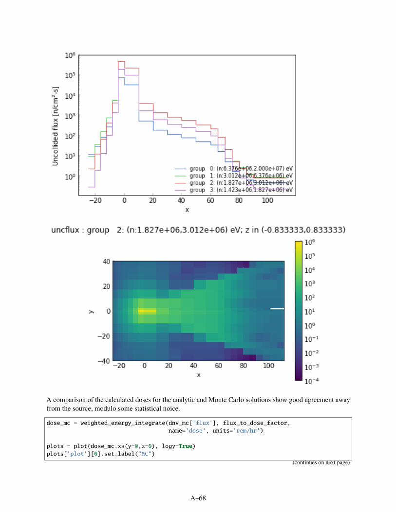
A comparison of the calculated doses for the analytic and Monte Carlo solutions show good agreement awayfrom the source, modulo some statistical noice.
dose_mc = weighted_energy_integrate(dnv_mc['flux'], flux_to_dose_factor,name='dose', units='rem/hr')
plots = plot(dose_mc.xs(y=0,z=0), logy=True)plots['plot'][0].set_label("MC")
(continues on next page)
A–68
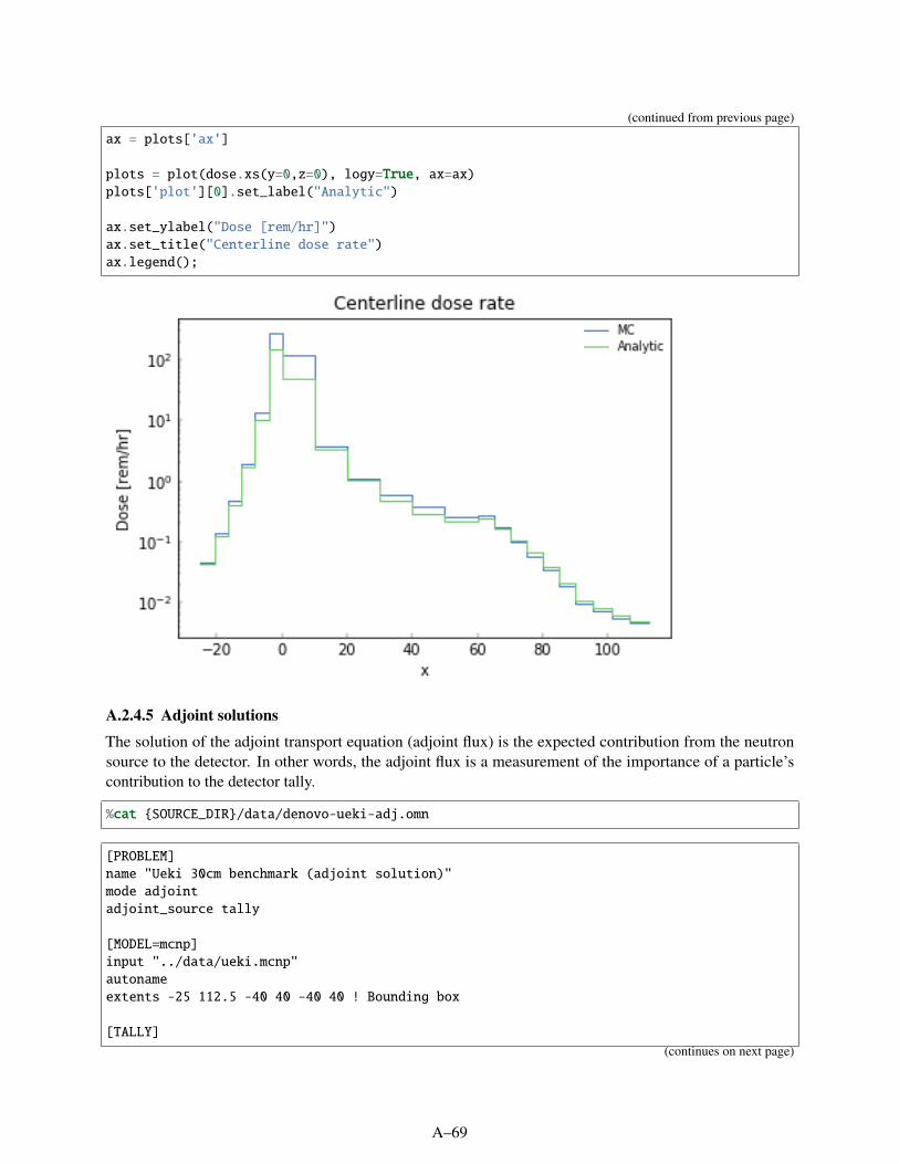
(continued from previous page)
ax = plots['ax']
plots = plot(dose.xs(y=0,z=0), logy=True, ax=ax)plots['plot'][0].set_label("Analytic")
ax.set_ylabel("Dose [rem/hr]")ax.set_title("Centerline dose rate")ax.legend();
A.2.4.5 Adjoint solutions
The solution of the adjoint transport equation (adjoint flux) is the expected contribution from the neutronsource to the detector. In other words, the adjoint flux is a measurement of the importance of a particle’scontribution to the detector tally.
%cat SOURCE_DIR/data/denovo-ueki-adj.omn
[PROBLEM]name "Ueki 30cm benchmark (adjoint solution)"mode adjointadjoint_source tally
[MODEL=mcnp]input "../data/ueki.mcnp"autonameextents -25 112.5 -40 40 -40 40 ! Bounding box
[TALLY]
(continues on next page)
A–69

(continued from previous page)
[TALLY][CELL response]cells 3
[PHYSICS=mg]mg_lib "v7-28n19g"mode npn_order 0disable_upscattering true
[DENOVO]method scx -25 5i 0 5i 60 5i 90 3i 112.5y -40 2i -25 2i -2.5 2i 2.5 2i 25 2i 40z -40 2i -25 2i -2.5 2i 2.5 2i 25 2i 40
[DENOVO][SOLVER=fixed]
[.][WITHIN_GROUP]verbosity nonemax_iterations 10
[DENOVO][QUADRATURE]num_azi 2num_polar 2
[RUN=mpi]np 4
[PRE][PRE][PLOT lateral]origin -25 0 -40size 127.5 80axis yrender true
!omnibus-run SOURCE_DIR/data/denovo-ueki-adj.omn
INFO: Starting Omnibus preprocessor, omnibus version 6.3.pre-b10 (branch 'omnibus-doc'→#98d73c8e on 2020MAR11)Loading problem db from Omnibus ASCII file...Loading Omnibus input file at /rnsdhpc/code/src/scale/Exnihilo/packages/Omnibus/driver/→example/data/denovo-ueki-adj.omn
...finished loading problem db from Omnibus ASCII fileLoading problem db from Python file...
...finished loading problem db from Python fileINFO: Set default for 'mpiexec_args' to '['-np', '4']' in '/run'Generating MCNP runtpe file...
...finished generating MCNP runtpe file>>> Loading nuclide data from processed MCNP libraries>>> Loading compositions from MCNP input>>> Loading nuclide data from processed MCNP libraries
(continues on next page)
A–70

(continued from previous page)
>>> Loading compositions from MCNP inputINFO: Set default for 'load_scl' to 'True' in '/comp'INFO: Set default for 'physics' to 'mg' in '/denovo'WARNING: The 'method' keyword is now 'equations' for SN discretization types. Changing→`method sc` to `equations sc`INFO: Set default for 'boundary' to ''_type': 'vacuum'' in '/denovo'INFO: Set default 'x_blocks 2' and 'y_blocks 2'INFO: Set default for 'z_blocks' to '2' in '/denovo/decomposition'INFO: Set default for 'quadrature' to 'qr' in '/denovo/quadrature'INFO: Set default for 'construction' to 'product' in '/denovo/quadrature'INFO: Set default for 'mat' to 'True' in '/denovo/output'INFO: Set default for 'source' to 'True' in '/denovo/output'INFO: Set default for 'uncflux' to 'True' in '/denovo/output'INFO: Set default for 'flux' to 'True' in '/denovo/output'INFO: Set default for 'upscatter_groups' to 'thermal' in '/denovo/solver'INFO: Method: snINFO: Equations: scINFO: Set default for 'solver' to 'gmres' in '/denovo/solver/within_group'INFO: Method: snINFO: Equations: scINFO: Set default for 'tolerance' to '0.001' in '/denovo/solver/within_group'INFO: Set default for 'preconditioner' to ''_type': 'none'' in '/denovo/solver/within_→group'INFO: Global Denovo mesh has 4950 cellsINFO: Renaming existing file denovo-ueki-adj.inp.xml to denovo-ueki-adj.inp-20200311-2236.→xmlINFO: Writing Omnibus input ParameterList to denovo-ueki-adj.inp.xml>>> Loading SCALE Standard Composition Library from /usr/local/scale/data/scale.rev40.→sclibGenerating geometry image...INFO: Saved geometry image at y=0 to 'lateral_y0.png'
...finished generating geometry imageINFO: Renaming existing file denovo-ueki-adj.pp.json to denovo-ueki-adj.pp-20200311-2236.→jsonINFO: Writing preprocessed file to denovo-ueki-adj.pp.jsonINFO: Writing processed ASCII input to 'denovo-ueki-adj.inp.omn'INFO: Launching Omnibus driver on 4 coresRunning Omnibus...INFO: Renaming existing file omnibus.out to omnibus-20200311-2236a.outINFO: Renaming existing file omnibus.err to omnibus-20200311-2236a.errWARNING: The Exnihilo software revision (r540) used to generate the input file differs→from this version being used to run it (r539).WARNING: This could cause internal consistency checks to unexpectedly fail, and it could→even lead to unexpected database value changes.WARNING: Please check your output very carefully after this run to make sure the→interpreted values match your input values.Building modelINFO: Loading SCALE Standard Composition Library from /usr/local/scale/data/scale.rev40.→sclibINFO: Loading compositions from MCNP inputINFO: Splitting compound 6000 into at% 6012: 0.9893, 6013: 0.0107INFO: Splitting compound 3006000 into at% 3006012: 0.9893, 3006013: 0.0107
(continues on next page)
A–71

(continued from previous page)
INFO: Creating default boundary mesh from (-25 -40 -40) to (112.5 40 40) for MCNP→geometryBuilding physics 'mg'INFO: Loading AMPX library at '/usr/local/scale/data/scale.rev12.xn28g19v7.1'INFO: Retained 3 of 455 nuclides on the master AMPX libraryINFO: Running XSProc on 2 cellsWARNING: Upscattering has been lumped into within-group scattering in the thermal groupsWARNING: Remapped 4 nuclide IDs: 6012->6000, 6013->6000, 3006012->3006000, 3006013->→3006000INFO: Truncating cross sections to groups [0, 28)Building talliesBuilding Denovo solver internalsRay tracing Denovo meshWARNING: Number of Z blocks (2) is not divisible into the number of z cells 15; reducing→to 1Mixing Denovo cross sectionsBuilding Denovo sourcesConstructing adjoint sources for DenovoWARNING: Tally 'response' has no multiplier specified in the HYBRID block; a flat→adjoint spectrum will be usedDiscretizing adjoint sources (1 cell tallies)Initializing Denovo solverINFO: Constructing Denovo state vector with 28 groups, 4950 cells, 1 moments, 1 unknowns→per cellRunning Denovo transport calculationAdjoint group 27 finished in 5 Belos Block GMRES iterations.Adjoint group 26 finished in 5 Belos Block GMRES iterations.Adjoint group 25 finished in 5 Belos Block GMRES iterations.Adjoint group 24 finished in 5 Belos Block GMRES iterations.Adjoint group 23 finished in 4 Belos Block GMRES iterations.Adjoint group 22 finished in 3 Belos Block GMRES iterations.Adjoint group 21 finished in 3 Belos Block GMRES iterations.Adjoint group 20 finished in 3 Belos Block GMRES iterations.Adjoint group 19 finished in 3 Belos Block GMRES iterations.Adjoint group 18 finished in 2 Belos Block GMRES iterations.Adjoint group 17 finished in 2 Belos Block GMRES iterations.Adjoint group 16 finished in 3 Belos Block GMRES iterations.Adjoint group 15 finished in 3 Belos Block GMRES iterations.Adjoint group 14 finished in 3 Belos Block GMRES iterations.Adjoint group 13 finished in 3 Belos Block GMRES iterations.Adjoint group 12 finished in 4 Belos Block GMRES iterations.Adjoint group 11 finished in 4 Belos Block GMRES iterations.Adjoint group 10 finished in 4 Belos Block GMRES iterations.Adjoint group 9 finished in 4 Belos Block GMRES iterations.Adjoint group 8 finished in 4 Belos Block GMRES iterations.Adjoint group 7 finished in 4 Belos Block GMRES iterations.Adjoint group 6 finished in 4 Belos Block GMRES iterations.Adjoint group 5 finished in 3 Belos Block GMRES iterations.Adjoint group 4 finished in 3 Belos Block GMRES iterations.Adjoint group 3 finished in 2 Belos Block GMRES iterations.Adjoint group 2 finished in 3 Belos Block GMRES iterations.INFO: Writing Silo file to 4 concurrent files using material volume fractions
(continues on next page)
A–72

(continued from previous page)
INFO: Removing SILO directory denovo_output_siloWriting Denovo HDF5 outputRun completeCleaning upAdjoint group 1 finished in 3 Belos Block GMRES iterations.Adjoint group 0 finished in 3 Belos Block GMRES iterations.
...finished running Omnibus in 2.7 secondsRunning Omnibus postprocessingLoading HDF5 file...INFO: Loaded Omnibus output data from 'denovo-ueki-adj.out.h5', problem name 'Ueki 30cm→benchmark (adjoint solution)', created on 2020MAR11 22:37 using SCALE version 6.3.pre-→b10 (branch 'omnibus-doc' #17579cc6 on 2020MAR10)
...finished loading HDF5 fileLoading HDF5 file...INFO: Loaded Omnibus output data from 'denovo-ueki-adj.out.h5', problem name 'Ueki 30cm→benchmark (adjoint solution)', created on 2020MAR11 22:37 using SCALE version 6.3.pre-→b10 (branch 'omnibus-doc' #17579cc6 on 2020MAR10)
...finished loading HDF5 fileWriting Denovo visualization file...INFO: Wrote Denovo visualization file to denovo-ueki-adj.denovo.xmf
...finished writing Denovo visualization fileBuilding RST summary...INFO: Wrote summary file to denovo-ueki-adj.rst
...finished building RST summary
dnv = load("denovo-ueki-adj.out.h5")['denovo'].extract()adj_flux = dnv['flux'].copy()adj_flux.name ='adjoint_flux'
Loading HDF5 file...INFO: Loaded Omnibus output data from 'denovo-ueki-adj.out.h5', problem name 'Ueki 30cm→benchmark (adjoint solution)', created on 2020MAR11 22:37 using SCALE version 6.3.pre-→b10 (branch 'omnibus-doc' #17579cc6 on 2020MAR10)
...finished loading HDF5 file
Plotting the adjoint flux shows how likely it is for particles at each point in space to contribute to the detector.Denovo predicts that the flux is of lowest importance in the paraffin block and of highest importance behindthe graphite shield.
plots = plot(adj_flux.xs(g=2,z=0.0), norm=norm)plots['ax'].title.set_position([.5, 1.25]);
A–73

A.2.5 DENOVO/SWORD INTEGRATION
This example demonstrates how to load and visualize a SWORD input file, create an Omnibus Denovo inputfor it that writes the angular flux and current, and post-process the output.
# Set up example environmentimport osfrom exnihilotools.matplotlib import screen_styleSOURCE_DIR = os.environ.get("SOURCE_DIR", ".")%matplotlib inlinescreen_style()
A.2.5.1 Visualize a GDML geometry
Loading a SWORD geometry reads a set of XML input files and calls Geant4 initialization routines to load acorresponding GDML geometry input.
from omnibus.raytrace.load import load_swordmodel = load_sword(os.path.join(SOURCE_DIR, "data", "btest5", "btest5.sword"))
Generating serialized SWORD model...INFO: Writing packed model to btest5.xdr
...finished generating serialized SWORD model
Omnibus includes tools to create color schemes based on the phyical compositions of the problem. TheColorMap.from_compositions method automatically assigns colors for common real-life materials suchas air, carbon-based life forms, and detector materials. The individual compositions from the model can alsobe explored to validate that Denovo is seeing the right nuclides, weight fractions, etc.
from omnibus.raytrace.colors import ColorMapcolors = ColorMap.from_compositions(model.compositions)colors.comps[1]._asdict()
A–74

'name': 'PMT_innerMetals','matid': 1,'density': 0.7,'temperature': 293.15,'zaid': array([ 6012, 6013, 13027, 15031, 16032, 16033, 16034, 16036, 24050,
24052, 24053, 24054, 25055, 26054, 26056, 26057, 26058, 28058,28060, 28061, 28062, 28064, 29063, 29065, 42092, 42094, 42095,42096, 42097, 42098, 42100], dtype=uint32),
'wtfrac': array([2.96790000e-05, 3.21000000e-07, 2.50000000e-01, 5.00000000e-05,4.74650000e-05, 3.80000000e-07, 2.14500000e-06, 1.00000000e-08,7.82100000e-04, 1.50820200e-02, 1.71018000e-03, 4.25700000e-04,1.70000000e-03, 4.11312650e-03, 6.45672898e-02, 1.49114030e-03,1.98443400e-04, 6.67153620e-03, 2.56986380e-03, 1.11710200e-04,3.56181000e-04, 9.07088000e-05, 8.64625000e-02, 3.85375000e-02,7.79100000e-02, 4.85625000e-02, 8.35800000e-02, 8.75700000e-02,5.01375000e-02, 1.26682500e-01, 5.05575000e-02]),
'depletable': False,'fissionable': False
from omnibus.raytrace.imager import Imagerimager = Imager(model.geometry,
lower=(-100, 0, -100),upper=(250, 0, 100),basis=(1, 0, 0),max_pixels=1024)
imager.names = [c.name for c in model.compositions]imager.colors = colorsimager.plot();
Rendering produces a faster, higher-resolution image but doesn’t show the extents or material names.
A–75

imager.render('rendered.png')from IPython.display import ImageImage(filename='rendered.png')
A.2.5.2 Execute Omnibus
The Omnibus input to this problem uses ANISN data (the multigroup data distributed with ADVANTG) andthe SWORD model loaded above. Inside the Denovo block it specifies to output both the current (first angularmoment) and the angular flux (actual discrete ordinates solution at each angle).
%cat SOURCE_DIR/data/btest.omn
[PROBLEM]name "Simple SWORD source-detector problem"mode forward
[MODEL=sword]input "btest5/btest5.sword"
[SOURCE=sword]
[PHYSICS=mg]anisn_lib "27n19g"pn_order 1disable_upscattering trueomit_zaid 8018mode ppemax 662e3
(continues on next page)
A–76

(continued from previous page)
[DENOVO]! Spatial grid with 'interpolation' keywordsx -100 2i -50 7i 50 8i 190 7i 210 2i 250y -100 2i -50 2i -20 -6 3i 6 20 2i 50 2i 100z -100 2i -50 -40 15i 40 50 2i 100
[DENOVO][OUTPUT]current trueangular_flux true
[DENOVO][QUADRATURE]order 16
[DENOVO][SOLVER=fixed][.][WITHIN_GROUP]verbosity none
[RUN=serial]
!omnibus-run SOURCE_DIR/data/btest.omn
INFO: Starting Omnibus preprocessor, omnibus version 6.3.pre-b10 (branch 'omnibus-doc'→#98d73c8e on 2020MAR11)Loading problem db from Omnibus ASCII file...Loading Omnibus input file at /rnsdhpc/code/src/scale/Exnihilo/packages/Omnibus/driver/→example/data/btest.omn
...finished loading problem db from Omnibus ASCII fileLoading problem db from Python file...
...finished loading problem db from Python fileGenerating serialized SWORD model...
...finished generating serialized SWORD modelINFO: Setting ANISN libraries based on data at /usr/local/advantg-data/27n19g.binINFO: Set default for 'load_scl' to 'False' in '/comp'INFO: Set default for 'physics' to 'mg' in '/denovo'INFO: Set default for 'boundary' to ''_type': 'vacuum'' in '/denovo'INFO: Set default 'x_blocks 1' and 'y_blocks 1'INFO: Set default for 'z_blocks' to '1' in '/denovo/decomposition'INFO: Set default for 'quadrature' to 'qr' in '/denovo/quadrature'INFO: Set default for 'construction' to 'levelsym' in '/denovo/quadrature'INFO: Set default for 'mat' to 'True' in '/denovo/output'INFO: Set default for 'source' to 'True' in '/denovo/output'INFO: Set default for 'uncflux' to 'True' in '/denovo/output'INFO: Set default for 'flux' to 'True' in '/denovo/output'INFO: Set default for 'upscatter_groups' to 'thermal' in '/denovo/solver'INFO: Method: snINFO: Equations: scINFO: Set default for 'solver' to 'gmres' in '/denovo/solver/within_group'INFO: Method: snINFO: Equations: scINFO: Set default for 'tolerance' to '0.001' in '/denovo/solver/within_group'INFO: Set default for 'preconditioner' to ''_type': 'none'' in '/denovo/solver/within_→group' (continues on next page)
A–77

(continued from previous page)
INFO: Global Denovo mesh has 13392 cellsINFO: Writing Omnibus input ParameterList to btest.inp.xmlINFO: Writing preprocessed file to btest.pp.jsonINFO: Writing processed ASCII input to 'btest.inp.omn'INFO: Launching Omnibus driver on 1 coresRunning Omnibus...WARNING: The Exnihilo software revision (r540) used to generate the input file differs→from this version being used to run it (r539).WARNING: This could cause internal consistency checks to unexpectedly fail, and it could→even lead to unexpected database value changes.WARNING: Please check your output very carefully after this run to make sure the→interpreted values match your input values.Building modelINFO: Loading Geant problem from GDML file at /rnsdhpc/code/src/scale/Exnihilo/packages/→Omnibus/driver/example/data/btest5/sword.gdmlINFO: Loading 19 elements from Geant4INFO: Loading nuclide data from Geant4 isotope librariesINFO: Loading 48 isotopes from Geant4WARNING: Nuclide data for 13027 was already set; ignoring and using existing dataWARNING: Nuclide data for 13027 was already set; ignoring and using existing dataINFO: Loading compositions from Geant4 material dataINFO: Creating default boundary mesh from (-12500 -12500 -12500) to (12500 12500 12500)→for Geant4 geometryBuilding physics 'mg'INFO: Loading ANISN attributes from /usr/local/advantg-data/27n19g.infoINFO: Loading ANISN zaid map from /usr/local/advantg-data/27n19g.zaidINFO: Loading ANISN cross sections from /usr/local/advantg-data/27n19g.binWARNING: Upscattering has been lumped into within-group scattering in the thermal groupsWARNING: Remapped 2 nuclide IDs: 6012->6000, 6013->6000WARNING: Omitted 1 nuclide IDs: 8018INFO: Truncating cross sections to groups [39, 46)Building sourcesBuilding Denovo solver internalsRay tracing Denovo meshMixing Denovo cross sectionsBuilding Denovo sourcesConstructing forward sources for DenovoDiscretizing SWORD sources (1 points)Initializing Denovo solverINFO: Constructing Denovo state vector with 7 groups, 13392 cells, 4 moments, 1 unknowns→per cellPerforming analytic first-collision source calculation on 1 sourcesRunning Denovo transport calculationForward group 0 finished in 3 Belos Block GMRES iterations.Forward group 1 finished in 3 Belos Block GMRES iterations.Forward group 2 finished in 3 Belos Block GMRES iterations.Forward group 3 finished in 4 Belos Block GMRES iterations.Forward group 4 finished in 5 Belos Block GMRES iterations.Forward group 5 finished in 7 Belos Block GMRES iterations.INFO: Writing Silo file to 1 concurrent files using material volume fractionsWriting Denovo HDF5 outputForward group 6 finished in 3 Belos Block GMRES iterations.
(continues on next page)
A–78

(continued from previous page)
Calculating angular fluxesRun completeCleaning up
...finished running Omnibus in 14.5 secondsRunning Omnibus postprocessingLoading HDF5 file...WARNING: Failed to build 'm' axis (via <bound method DataAxis.from_group of <class→'omnibus.data.axis.DataAxis'>>) for 'angular_flux' of '/denovo': "Unable to open→object (object 'mesh_m' doesn't exist)"INFO: Loaded Omnibus output data from 'btest.out.h5', problem name 'Simple SWORD source-→detector problem', created on 2020MAR11 22:38 using SCALE version 6.3.pre-b10 (branch→'omnibus-doc' #17579cc6 on 2020MAR10)
...finished loading HDF5 fileLoading HDF5 file...INFO: Loaded Omnibus output data from 'btest.out.h5', problem name 'Simple SWORD source-→detector problem', created on 2020MAR11 22:38 using SCALE version 6.3.pre-b10 (branch→'omnibus-doc' #17579cc6 on 2020MAR10)
...finished loading HDF5 fileWriting Denovo visualization file...INFO: Wrote Denovo visualization file to btest.denovo.xmf
...finished writing Denovo visualization fileBuilding RST summary...INFO: Wrote summary file to btest.rst
...finished building RST summary
A.2.5.3 Process results
from omnibus.formats.output import loaddnv = load("btest.out.h5")['denovo'].extract()
Loading HDF5 file...WARNING: Failed to build 'm' axis (via <bound method DataAxis.from_group of <class→'omnibus.data.axis.DataAxis'>>) for 'angular_flux' of '/denovo': "Unable to open→object (object 'mesh_m' doesn't exist)"INFO: Loaded Omnibus output data from 'btest.out.h5', problem name 'Simple SWORD source-→detector problem', created on 2020MAR11 22:38 using SCALE version 6.3.pre-b10 (branch→'omnibus-doc' #17579cc6 on 2020MAR10)
...finished loading HDF5 file
Uncollided flux
A good first step in analysis is to verify the source term: in this case, checking that it is nonzero only in thehighest group. The xs command slices the data with the group index for a single group, or with a Pythonslice object to get a range of groups. (a[slice(1,None)] is equivalent to a[1:].)
import numpy as np
uncflux = dnv['uncflux']print(np.count_nonzero(uncflux.xs(g=0)))print(np.count_nonzero(uncflux.xs_by_index(g=slice(1,None))))
A–79

133920
A lineout plot along y = z = 0 for the source group clearly shows the attenuation through the detector atx = 200.
from omnibus.data import plot
plots = plot(uncflux.xs(y=0.0, z=0.0, g=0), logy=True);plots['ax'].set_ylabel('');
The “scalar flux” is the zeroth angular moment of the angular flux:
φ =
∫4πψ(~x, ~Ω)dΩ
It is effectively a measure of particle density, and is used in calculating reaction rates.
The following command extracts the data at the origin. Since the only remaining data axis is energy, the plotfunction will render a step plot of the group-average fluxes.
Flux
import matplotlib.pyplot as plt
flux = dnv['flux']origin_spectrum = flux.xs(x=0, y=0, z=0)
plots = plot(origin_spectrum, logy=True)ax = plots['ax']
(continues on next page)
A–80

(continued from previous page)
# Rotate the X tick labelsplt.setp(ax.get_xticklabels(), rotation=90);ax.set_title(ax.get_ylabel())ax.set_ylabel("Particle flux (p/cm^2-s)");
The next command accesses the flux at group index 3 (not 3 eV!) at z = 0. With the resulting x-y data, theplotter renders a pseudocolor plot. Specifying a special value for norm renders the colors on a logarithmicscale.
from matplotlib.colors import LogNorm
plot(flux.xs(z=0., g=3), norm=LogNorm());
A–81

Net current
The current field is the “net current”, the first moment of the angular flux:
~J =
∫4π
~Ωψ(~x, ~Ω)dΩ .
It is stored as an energy, space, and direction-dependent field; the data attribute is the pointer to the HDF5data.
The current describes the net flow rate of particles traveling through a point in space. The following commandprint the dimensionality of the current:
current = dnv['current']print(", ".join("=".format(d,s)
for (d,s) in zip(current.dims, current.shape)))
g=7, z=24, y=18, x=31, dir=3
The following command takes a slice at the energy group for photons at 1e5 eV, at the XYZ coordinates of(7, 3, 5). The resulting vector is the current along the (x, y, z) directions.
sliced = current.xs(x=7.0, y=3.0, z=5.0, g=('p', 1e5))print(sliced.mesh('dir'))sliced
['x' 'y' 'z']
Other slices are of course possible. This command plots the multigroup net current at a particular point:
plot(current.xs(x=7.0, y=3.0, z=5.0, dir='x'), logy=True);
A–82

The full angle-dependent particle flux can be approximated by using the angular moments. This is the PN
approximation.
ψ(~x, ~Ω) ≈1
4π(φ(~x) + 3~Ω · ~J(~x))
However, a much more accurate representation of the angular flux can be obtained directly from Denovo.
Angular flux
The full S N flux can be saved by setting angular_flux true inside the [DENOVO][OUTPUT] block. Thisoption requires careful consideration due to the disk space requirements: for an S 16 quadrature set, it will be288 times as large as the scalar flux.
# Extract the angle-dependent flux averaged over a single spatial point in one energy→groupflux = dnv['angular_flux']angle_flux = flux.xs(g=('p', 7e5), x=200.0, y=1.5 , z=2.5)angle_flux
angles = dnv.quadrature_angles.extract()angles
These tools can perform a wide range of functions. For example, numpy logical expressions can determineall the angle indices in the +z direction, and matplotlib can then create a scatter plot of the angluar fluxesprojected into the xy plane.
A–83

z_slice = angles.data[:,2] > 0
plt.scatter(angles[z_slice,0], angles[z_slice,1],c=np.abs(angle_flux.data[z_slice]),norm=LogNorm(), cmap='viridis', edgecolor='none')
plt.axis('square');plt.colorbar();
A.2.6 EXNIHILO MESH INPUT DEFINITION
These small problems are used in the Denovo unit tests. The output files should be saved to Geometria/mesh/rect/test/data.
# Set up plotting%matplotlib inlinefrom exnihilotools.matplotlib import screen_stylescreen_style()
A.2.6.1 Problem A
This is a 3D problem with a volume source.
from omnibus.mesh import Meshfrom omnibus.formats.meshmodel import MeshModelFileimport numpy as np
mesh = Mesh(x=np.arange(21), y=np.arange(16), z=np.arange(11))problem = MeshModelFile.from_mesh(mesh)
If the mesh axes were irregular, then a snippet of code like the following could be used to ‘slice’ the matidsmore easily. In order to select a view of the data to assign matids, we have to use standard python sliceobjects or integers.
A–84

from omnibus.data import simplify_logical_slice
x_centers = problem['matids'].axis('x').centersdef x_slice(xmin, xmax):
return simplify_logical_slice((x_centers >= xmin) & (x_centers <= xmax))print(x_slice(3,10))
slice(3, 10, None)
The xs_by_index method selects subsets of the mesh, either multiple elements or a single element, alongmultiple axes. The following chunks of code are used to assign materials and a source definition.
from omnibus.data import plot
matids = problem['matids']zmats = matids.xs_by_index(z=slice(1,))zmats.xs_by_index(y=slice(5, 15)).data[:] = 1zmats.xs_by_index(x=slice(0,15), y=slice(10,15)).data[:] = 2zmats.xs_by_index(y=slice(3,5)).data[:] = 2
plot(matids.xs(x=0.5), edgecolor='gray', linewidth=0.25);
src = problem['volsrc']spectra = src['spectra']
num_groups = 3spectra.resize(2, num_groups)spectra.get_spectrum(0)[:] = [0.6, 0.3, 0.1]spectra.get_spectrum(1)[:] = [0.4, 0.2, 0.4]
srcids = src['ids']
(continues on next page)
A–85

(continued from previous page)
srcids.xs_by_index(y=slice(3,5), z=slice(1,9)).data[:] = 1plot(srcids.xs(z=1.0));
strength = src['strength']
q0 = np.linspace(0.5, 1.5, 15)q1 = np.linspace(0.5, 1.5, 20)
strength.xs_by_index(x=slice(0,15), y=slice(10,15), z=slice(1,10)).data[:] = q0strength.xs_by_index(y=slice(3,5), z=slice(1,10)).data[:] = q1
plot(strength.xs(z=1.0));
A–86

Now that the problem is constructed, it can be written to disk for later use in Omnibus:
import h5pyfrom omnibus.data import dump_root
with h5py.File("simple-3d.h5", 'w') as f:dump_root(problem, f)
INFO: Omitting empty point source
A.2.6.2 Problem B
This 2D problem is constructed similarly to the previous one.
from omnibus.mesh import Mesh2D
# Make the meshmesh = Mesh2D(x=np.arange(21), y=np.arange(16))problem = MeshModelFile.from_mesh(mesh)
# Assign data directly: note that the axes are ordered# in reverse, so slice indices must also be reversedmatids = problem['matids'].dataassert problem['matids'].dims == ['y', 'x']matids[5:15,:] = 1matids[10:15,0:15] = 2matids[3:5,:] = 2
src = problem['volsrc']spectra = src['spectra']
(continues on next page)
A–87

(continued from previous page)
spectra.resize(2, 3)spectra.get_spectrum(0)[:] = [0.6, 0.3, 0.1]spectra.get_spectrum(1)[:] = [0.4, 0.2, 0.4]
srcids = src['ids'].datasrcids[3:5,:] = 1
strength = src['strength'].data
q0 = np.linspace(0.5, 1.5, 15)q1 = np.linspace(0.5, 1.5, 20)
strength[10:15,0:15] = q0strength[3:5,:] = q1
with h5py.File("simple-2d.h5", 'w') as f:dump_root(problem, f)
INFO: Omitting empty point source
A.2.6.3 Problem C
This 3D problem includes mix tables and does not specify a source definition.
import matplotlib.pyplot as pltfrom omnibus.formats.meshmodel import MixTable
mesh = Mesh(x=np.arange(17), y=np.arange(9), z=np.arange(9))problem = MeshModelFile.from_mesh(mesh)
matids = problem['matids'].data
# Note that dimensions are z/y/xmatids[:] = 0matids[:6,2:6,4:13] = 2 # mixturematids[3:5,3:5,5:12] = 1 # pure
(fig, ax) = plt.subplots()ax.pcolormesh(mesh.x, mesh.y, matids[4,:,:], edgecolor=(.5,.5,.5))ax.set_aspect(1.0);
# Build a mix tablemix_table = np.array([[1.0, 0.0],
[0.0, 1.0],[0.5, 0.5]])
problem['mixtable'] = MixTable.from_table(mix_table)
# Print the COO representation it madeprint(problem['mixtable'].data)
(continues on next page)
A–88

(continued from previous page)
# Save to diskwith h5py.File("mixed-3d.h5", 'w') as f:
dump_root(problem, f)
INFO: Omitting empty volume sourceINFO: Omitting empty point source
[(0, 0, 1. ) (1, 1, 1. ) (2, 0, 0.5) (2, 1, 0.5)]
A.2.6.4 Uniform source and material
mesh = Mesh(x=np.arange(10, dtype='f8'),y=np.arange(10, dtype='f8'),z=np.arange(10, dtype='f8'))
problem = MeshModelFile.from_mesh(mesh)
matids = problem['matids'].datamatids[:] = 0
# Define source spectrasrc = problem['volsrc']spectra = src['spectra']spectra.resize(1,1)spectra.get_spectrum(0)[:] = [1.0]
# Assign IDs and source strengthssrcids = src['ids'].datasrcids[:] = 0strength = src['strength'].datastrength[:] = 1.0
# Save to diskwith h5py.File("uniform-3d.h5", 'w') as f:
dump_root(problem, f)
A–89

INFO: Omitting empty point source
A.2.6.5 Both point and volume sources
The input file constructed here will contain both volume and point sources.
mesh = Mesh(x=np.arange(15, dtype='f8'),y=np.arange(9, dtype='f8'),z=np.arange(5, dtype='f8'))
problem = MeshModelFile.from_mesh(mesh)
# Add volume sourcessrc = problem['volsrc']spectra = src['spectra']
num_groups = 3spectra.resize(4, num_groups)spectra.get_spectrum(0)[:] = [0.6, 0.3, 0.1]spectra.get_spectrum(1)[:] = [0.4, 0.2, 0.4]spectra.get_spectrum(2)[:] = [0.3, 0.5, 0.2]spectra.get_spectrum(3)[:] = [1.0, 0.0, 0.0]
srcids = src['ids'].datasrcids[:3,6:8,0:2] = 1srcids[:,2:6,4:8] = 1
plot(src['ids'].xs(z=1.0));
Next, set varying strengths in the different cells.
strength = src['strength'].datastrength[:3,6:8,0:2].flat = np.linspace(0.1, 1.1, 3*2*2)
(continues on next page)
A–90

(continued from previous page)
strength[:,2:6,4:8].flat = np.linspace(0.5, 2.5, 4*4*4)
plot(src['strength'].xs(z=1.0));
Finally, add the point sources and write the problem to disk.
# Add point sourcespointsrc = problem['ptsrc']
# Points are in X,Y,Z and use the same spectra as the volume sourcepointsrc.resize(2, spectra.num_groups)pointsrc.set_point(0, (10.5, 5.5, 0.5), 3.45, spectra.get_spectrum(2))pointsrc.set_point(1, (13.5, 7.5, 3.5), 2.34, spectra.get_spectrum(3))
with h5py.File("points.h5", 'w') as f:dump_root(problem, f)
A.3 MULTIGROUP DATA EXPLORATION
These examples show how to use Exnihilo’s Python bindings (page 2) to extract and visualize multigroup andother Denovo-related data.
A.3.1 CROSS SECTION GENERATION
This example demonstrates generating and visualizing multigroup cross sections using the Exnihilo pythoninterface.
# Set up example%matplotlib inline%load_ext wurlitzerfrom exnihilotools.matplotlib import screen_stylescreen_style()
A–91
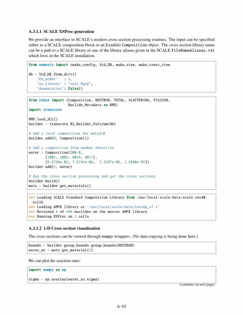
A.3.1.1 SCALE XSProc generation
We provide an interface to SCALE’s modern cross section processing routines. The input can be specifiedeither as a SCALE composition block or an Exnihilo Composition object. The cross section library namecan be a path to a SCALE library or one of the library aliases given in the SCALE FileNameAliases.txtwhich lives in the SCALE installation.
from nemesis import cmake_config, Std_DB, make_view, make_const_view
db = Std_DB.from_dict('Pn_order' : 3,'xs_library' : "test-8grp",'downscatter': False)
from robus import (Composition, NEUTRON, TOTAL, SCATTERING, FISSION,Nuclide_Metadata as NMD)
import transcore
NMD.load_SCL()builder = transcore.XS_Builder_Fulcrum(db)
# Add a 'void' composition for matid=0builder.add(0, Composition())
# Add a composition from number densitieswater = Composition(300.0,
[1001, 1002, 8016, 8017],[6.6728e-02, 7.6745e-06, 3.3287e-02, 1.2680e-05])
builder.add(2, water)
# Run the cross section processing and get the cross sectionsbuilder.build()mats = builder.get_materials()
>>> Loading SCALE Standard Composition Library from /usr/local/scale/data/scale.rev40.→sclib>>> Loading AMPX library at '/usr/local/scale/data/test8g_v7.1'>>> Retained 4 of 449 nuclides on the master AMPX library>>> Running XSProc on 1 cells
A.3.1.2 1-D Cross section visualization
The cross sections can be viewed through numpy wrappers. (No data copying is being done here.)
bounds = builder.group_bounds.group_bounds(NEUTRON)water_xs = mats.get_material(2)
We can plot the reaction rates:
import numpy as np
sigma = np.asarray(water_xs.sigma)
(continues on next page)
A–92

(continued from previous page)
sigma_s = np.asarray(water_xs.sigma_x(SCATTERING))#sigma_f = np.asarray(water_xs.sigma_x(FISSION))
import matplotlib.pyplot as pltfrom matplotlib.colors import Normalize, LogNormfrom exnihilotools.matplotlib.artists import plot_multigroupfrom exnihilotools.matplotlib.axes import grid_groups, annotate_groups
(fig, ax) = plt.subplots(subplot_kw=dict(xscale='log'))plot_multigroup(ax, bounds, sigma, label='total')plot_multigroup(ax, bounds, sigma_s, label='scatter')ax.legend()grid_groups(ax, bounds)annotate_groups(ax, bounds);
A.3.1.3 Scattering matrix visualization
The scattering matrix with all the requested angular moments (g, g′, l) can be pulled directly from the crosssection container. In this example, there are 4 moments since we requested P3 scattering.
scat = water_xs.scatter_matrixscat.shape
(8, 8, 4)
plt.matshow(scat[:,:,0], cmap='viridis', norm=LogNorm())plt.title("$P_0$ scattering")plt.colorbar();
A–93

scat[3,3,:]
array([0.06847651, 0.03386217, 0.01825174, 0.00616768])
A scattering cross section that’s perfectly forward-peaked
σs(µ) = δ(µ − 1)
will have σ0 = σ1 = σ2 = ....
plt.matshow(scat[:,:,1] / np.ma.masked_equal(scat[:,:,0], 0.0), cmap='rb_linear',→norm=Normalize(-1,1))plt.title(r"Forward peakness ($\sigma_1 / \sigma_0$)")plt.colorbar();
A–94

Legendre coefficents
The numpy package has a function for evaluating a Legendre series at a series of points. This allows us toeasily visualize the reconstructed scattering as a function of angle.
from numpy.polynomial.legendre import legvalx = np.linspace(-1, 1, 128)
def plot_legendre(ax, coeffs, norm=False, **kwargs):if norm:
coeffs = coeffs / coeffs[0]ax.plot(x, legval(x, coeffs), **kwargs)#ax.set_ylim(-1, 1)ax.grid()return ax
(fig, ax) = plt.subplots()plot_legendre(ax, [0,0,0,1]);ax.set_title("Legendre function $P_3$");
A–95

g = 0(fig, ax) = plt.subplots() # subplot_kw=dict(yscale='log'))
# Loop through all the outscatter groups for the highest-energy xsfor gp in range(8):
plot_legendre(ax, scat[gp, g, :], label=r'$:d \to :d$'.format(g,gp))ax.legend();ax.set_title(r'$\sigma_s(\mu)$ for the highest-energy group');
A–96

A.3.2 INFINITE-MEDIUM CRITICALITY SEARCH
Simple linear algebra can solve for the keff of an infinite homogeneous medium given multigroup crosssections. This advanced example ties together some low-level Exnihilo utilities (in Robus and Transcore)with python packages numpy and scipy.
This example’s objective is to determine a critical homogeneous mixture of 5%-enriched UO2 and water. Thefinal result will be a composition that can then be used for unit testing.
# Set up example%matplotlib inline%load_ext wurlitzerfrom exnihilotools.matplotlib import screen_stylescreen_style()
A.3.2.1 Construct compositions
There are some utility functions in Exnihilo that build UO2 compositions and can calculate mixtures.
from robus import (Composition, Comp_Mixer, NEUTRON, TOTAL, SCATTERING, FISSION, NU_→FISSION,
Nuclide_Metadata as NMD)
NMD.load_SCL()
temperature = 300.0density = 10.257enrichment_pcwt = 5.0uo2 = Comp_Mixer.get_enriched_uo2(temperature, density, enrichment_pcwt)
density = 1.0h2o = Composition(temperature, density, [1001, 8016],
[0.11191539275728472, 0.8880846072427153]);
>>> Loading SCALE Standard Composition Library from /usr/local/scale/data/scale.rev40.→sclib
MIX_DENSITY = 2.0 # Irrelevant for infinite mediumdef mix(fuel, mod, frac_fuel):
return Comp_Mixer.mix(MIX_DENSITY, fuel, mod, frac_fuel, Comp_Mixer.MIX_BY_WEIGHT)
mixture = mix(uo2, h2o, frac_fuel=0.5)mixture._asdict()
'name': '','matid': 3,'temperature': 300.0,'density': 2.0,'fissionable': True,'depletable': True,'zaid': array([ 1001, 8016, 92234, 92235, 92236, 92238], dtype=uint32),'wtfrac': array([5.59576964e-02, 5.03307698e-01, 1.96126900e-04, 2.20367303e-02,
1.01368959e-04, 4.18400380e-01])
A–97

A.3.2.2 Calculating k of a composition
The multigroup approximation allows k-effective of a homogeneous composition to be calculated straightfor-wardly by explicitly constructing a matrix whose largest eigenvalue is k. The first step of this process is touse SCALE’s XSProc code via the XS_Builder_Fulcrum class to collapse an eight-group test library into ahomogeneous set of cross sections, which are then converted into native numpy arrays.
from nemesis import Std_DB, make_view, make_const_viewimport transcoreimport numpy as np
# Set up the builderdb = Std_DB.from_dict(
'Pn_order' : 0,'xs_library' : "v7-56",'downscatter': False)
builder = transcore.XS_Builder_Fulcrum(db)builder.add(0, mixture)
# Generate and retrieve cross sectionsbuilder.build()bounds = builder.group_bounds.group_bounds(NEUTRON)mats = builder.get_materials()mixture_xs = mats.get_material(0)
# Extract cross sections as native Python objectssigma_t = np.asarray(mixture_xs.sigma)sigma_s = np.asarray(mixture_xs.scatter_matrix)[:,:,0] # P0 moments of scattering matrixnu_sigma_f = np.asarray(mixture_xs.sigma_x(NU_FISSION))chi = np.asarray(mixture_xs.chi)
>>> Loading AMPX library at '/usr/local/scale/data/scale.rev04.xn56v7.1'>>> Retained 6 of 457 nuclides on the master AMPX library>>> Running XSProc on 1 cells
from exnihilotools.matplotlib.artists import plot_multigroupfrom exnihilotools.matplotlib.axes import grid_groups, annotate_groups
Here is the scattering matrix:
import matplotlib.pyplot as pltfrom matplotlib.colors import LogNormplt.matshow(sigma_s, norm=LogNorm());
A–98

The multigroup neutron balance equation (with fission and no extraneous source) is:
Σt,gφg =
G−1∑g′=0
Σs,g′→gφg′ +1kχg
G−1∑g′=0
νΣ f ,g′φg′ ,
which can be written as the linear algebra equation
TΦ = S Φ +1kχ f T Φ ,
where f T Φ is the fission source strength density (a scalar), S is the scattering matrix, and T is diag(Σt).
Simple manipulations yield an explicit eigenvalue equation
kΦ = (T − S )−1χ f T Φ .
The following code constructs the right-hand-side matrix and solves for its eigenvalues:
t_minus_s = (np.diag(sigma_t) - sigma_s)chi_nusig = np.outer(chi, nu_sigma_f)final_matrix = np.matmul(np.linalg.inv(t_minus_s), chi_nusig)(all_k, all_phi) = np.linalg.eig(final_matrix)
def max_eigenvalue(all_k, all_phi):# Find k-effk_idx = np.argmax(all_k)k = all_k[k_idx].real# Get the corresponding eigenvector and make sure it's positivephi = all_phi[:,k_idx].realif np.min(phi) < 0 and np.max(phi) <= 0:
phi *= -1
(continues on next page)
A–99

(continued from previous page)
return (k, phi)
(k, phi) = max_eigenvalue(all_k, all_phi)
print("K-eff is", k)
K-eff is 1.3696586943136313
delta_lethargy = -np.diff(np.log(bounds))(fig, ax) = plt.subplots(subplot_kw=dict(xscale='log', yscale='log'))plot_multigroup(ax, bounds, phi / delta_lethargy)ax.set_xlabel('Energy (eV)')ax.set_ylabel('Flux per unit lethargy')ax.set_yticks([])ax.set_yticklabels([]);
A.3.2.3 Finding criticality
The above process successfully calculates the eigenvalue (keff) and eigenvector (flux spectrum) given a singlescalar, the fuel fraction. It is condensed below into a single function calc_k, which is the workhorse of afunction calc_reactivity that gives the reactivity,
ρ =k − 1
k,
as a function of the fuel fraction. Solving for the single root ρ = 0 is therefore solving for the critical fuelfraction.
Using an 8-group test library instead of the 56-group library above substantially reduces the calculation time.
A–100

db = Std_DB.from_dict('Pn_order' : 0,'xs_library' : "test-8grp",'downscatter': False)
def calc_k(frac_fuel):mixture = mix(uo2, h2o, frac_fuel=frac_fuel)builder = transcore.XS_Builder_Fulcrum(db)builder.add(0, mixture)
# Generate and retrieve cross sectionsbuilder.build()bounds = builder.group_bounds.group_bounds(NEUTRON)mats = builder.get_materials()mixture_xs = mats.get_material(0)
# Get cross sections as numpy objectssigma_t = np.asarray(mixture_xs.sigma)sigma_s = np.asarray(mixture_xs.scatter_matrix)[:,:,0] # P0 moments of scattering
→matrixnu_sigma_f = np.asarray(mixture_xs.sigma_x(NU_FISSION))chi = np.asarray(mixture_xs.chi)
# Construct fission-transport matrixt_minus_s = (np.diag(sigma_t) - sigma_s)chi_nusig = np.outer(chi, nu_sigma_f)final_matrix = np.matmul(np.linalg.inv(t_minus_s), chi_nusig)
# Calculate eigenvalue and eigenvector(all_k, all_phi) = np.linalg.eig(final_matrix)return max_eigenvalue(all_k, all_phi)
def calc_reactivity(frac_fuel):if frac_fuel <= 0:
k = 0rho = -np.inf
elif frac_fuel >= 1:k = rho = np.inf
else:assert not np.isnan(frac_fuel)(k, _) = calc_k(frac_fuel)rho = (k - 1.0) / k
print("frac_fuel:f fuel -> k=k:.5f (rho=rho:g)".format(**locals()))return rho
Finally, we use the optimization toolkit from scipy to find the root, giving our final answer.
from scipy.optimize import root_scalar
result = root_scalar(calc_reactivity, method='brentq', bracket=(0,1), x0=0.5, rtol=1e-4)print(result)frac_fuel = result.root
(continues on next page)
A–101

(continued from previous page)
print("Final fuel fraction:", frac_fuel)
0.000000 fuel -> k=0.00000 (rho=-inf)1.000000 fuel -> k=inf (rho=inf)0.500000 fuel -> k=1.47630 (rho=0.322633)
>>> Loading AMPX library at '/usr/local/scale/data/test8g_v7.1'>>> Retained 6 of 449 nuclides on the master AMPX library>>> Running XSProc on 1 cells>>> Loading AMPX library at '/usr/local/scale/data/test8g_v7.1'>>> Retained 6 of 449 nuclides on the master AMPX library>>> Running XSProc on 1 cells
0.250000 fuel -> k=1.03433 (rho=0.0331943)0.125000 fuel -> k=0.64392 (rho=-0.552994)0.242922 fuel -> k=1.01642 (rho=0.016158)
>>> Loading AMPX library at '/usr/local/scale/data/test8g_v7.1'>>> Retained 6 of 449 nuclides on the master AMPX library>>> Running XSProc on 1 cells>>> Loading AMPX library at '/usr/local/scale/data/test8g_v7.1'>>> Retained 6 of 449 nuclides on the master AMPX library>>> Running XSProc on 1 cells>>> Loading AMPX library at '/usr/local/scale/data/test8g_v7.1'>>> Retained 6 of 449 nuclides on the master AMPX library>>> Running XSProc on 1 cells
0.236399 fuel -> k=0.99956 (rho=-0.000440535)0.236572 fuel -> k=1.00000 (rho=1.41172e-06)0.236560 fuel -> k=0.99997 (rho=-3.22038e-05)
converged: Trueflag: 'converged'
function_calls: 9iterations: 8
root: 0.23657180483813495Final fuel fraction: 0.23657180483813495
>>> Loading AMPX library at '/usr/local/scale/data/test8g_v7.1'>>> Retained 6 of 449 nuclides on the master AMPX library>>> Running XSProc on 1 cells>>> Loading AMPX library at '/usr/local/scale/data/test8g_v7.1'>>> Retained 6 of 449 nuclides on the master AMPX library>>> Running XSProc on 1 cells
The final answer, the critical fuel mixture, is thus:
mix(uo2, h2o, frac_fuel=frac_fuel)._asdict()
A–102

'name': '','matid': 11,'temperature': 300.0,'density': 2.0,'fissionable': True,'depletable': True,'zaid': array([ 1001, 8016, 92234, 92235, 92236, 92238], dtype=uint32),'wtfrac': array([8.54393663e-02, 7.06029871e-01, 9.27961893e-05, 1.04265381e-02,
4.79620753e-05, 1.97963466e-01])
A.4 SHIFT
A.4.1 DEBUGGING GEOMETRY PROBLEMS IN SHIFT
It is not unusual to make an error when constructing a geometry model. This example gives a few usefulprocedures for tracking down geometry errors.
# Set up example environmentimport osfrom exnihilotools.matplotlib import screen_styleSOURCE_DIR = os.environ.get("SOURCE_DIR", ".")%matplotlib inlinescreen_style()
A.4.1.1 Construct compositions via the SCL
Since this test geometry is a Geometria XML input, it doesn’t natively support composition definitions. Hereis one of the many ways to define compositions: loading them using the robus Python wrappers from theSCALE standard composition library, and then writing them to an HDF5 file which is then specified in theOmnibus input.
from robus import (Composition, load_scl_compositions, load_hdf5_compositions, save_hdf5_→compositions)
# Load the compositions into a dictionary (the method returns a vector of Composition→objects)scl_comps = dict((c.name, c) for c in load_scl_compositions())# Display a couple of them in alphabetical orderprint(sorted(scl_comps.keys())[:5])
['al2o3', 'b4c', 'balsa', 'benzene', 'beo']
# Pick a few compositionsexport_comps = [scl_comps[k] for k in ["dry-air", "ss304", "water"]]# Dump them to an HDF5 filesave_hdf5_compositions(os.path.join(SOURCE_DIR, "data", "buggy.comp.h5"), export_comps)
A.4.1.2 Run Shift through Omnibus
With a pre-constructed (but broken) geometry file, an Omnibus input file, and the set of compositions justgenerated, Omnibus can be run to see what happens.
A–103
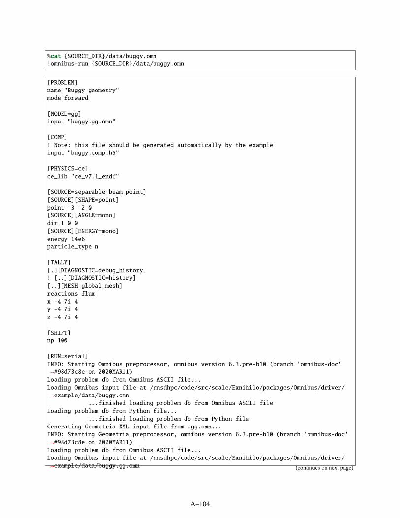
%cat SOURCE_DIR/data/buggy.omn!omnibus-run SOURCE_DIR/data/buggy.omn
[PROBLEM]name "Buggy geometry"mode forward
[MODEL=gg]input "buggy.gg.omn"
[COMP]! Note: this file should be generated automatically by the exampleinput "buggy.comp.h5"
[PHYSICS=ce]ce_lib "ce_v7.1_endf"
[SOURCE=separable beam_point][SOURCE][SHAPE=point]point -3 -2 0[SOURCE][ANGLE=mono]dir 1 0 0[SOURCE][ENERGY=mono]energy 14e6particle_type n
[TALLY][.][DIAGNOSTIC=debug_history]! [..][DIAGNOSTIC=history][..][MESH global_mesh]reactions fluxx -4 7i 4y -4 7i 4z -4 7i 4
[SHIFT]np 100
[RUN=serial]INFO: Starting Omnibus preprocessor, omnibus version 6.3.pre-b10 (branch 'omnibus-doc'→#98d73c8e on 2020MAR11)Loading problem db from Omnibus ASCII file...Loading Omnibus input file at /rnsdhpc/code/src/scale/Exnihilo/packages/Omnibus/driver/→example/data/buggy.omn
...finished loading problem db from Omnibus ASCII fileLoading problem db from Python file...
...finished loading problem db from Python fileGenerating Geometria XML input file from .gg.omn...INFO: Starting Geometria preprocessor, omnibus version 6.3.pre-b10 (branch 'omnibus-doc'→#98d73c8e on 2020MAR11)Loading problem db from Omnibus ASCII file...Loading Omnibus input file at /rnsdhpc/code/src/scale/Exnihilo/packages/Omnibus/driver/→example/data/buggy.gg.omn (continues on next page)
A–104

(continued from previous page)
...finished loading problem db from Omnibus ASCII fileINFO: Writing Geometria input ParameterList to buggy.gg.xml
...finished generating Geometria XML input file from .gg.omnINFO: Set default for 'fissionable_only' to 'False' in '/source/beam_point'INFO: Set default for 'mode' to 'n' in '/physics/ce'INFO: Set default for 'xs_cache' to 'tot' in '/physics/ce'INFO: Set default for 'xs_accel' to 'True' in '/physics/ce'INFO: Set default for 'fission_neutrons' to 'True' in '/physics/ce/fission'INFO: Set default for 'load_scl' to 'True' in '/comp'INFO: Set default for 'decomposition' to ''_type': 'none'' in '/shift'INFO: Set default for 'verbosity' to 'low' in '/shift/transporter'INFO: Set default for 'method' to 'roulette' in '/shift/vr'INFO: Writing Omnibus input ParameterList to buggy.inp.xmlINFO: Writing preprocessed file to buggy.pp.jsonINFO: Writing processed ASCII input to 'buggy.inp.omn'INFO: Launching Omnibus driver on 1 coresRunning Omnibus...WARNING: The Exnihilo software revision (r540) used to generate the input file differs→from this version being used to run it (r539).WARNING: This could cause internal consistency checks to unexpectedly fail, and it could→even lead to unexpected database value changes.WARNING: Please check your output very carefully after this run to make sure the→interpreted values match your input values.Building modelINFO: Loading SCALE Standard Composition Library from /usr/local/scale/data/scale.rev40.→sclibINFO: Loading compositions from /rnsdhpc/code/src/scale/Exnihilo/packages/Omnibus/driver/→example/data/buggy.comp.h5INFO: Creating default boundary mesh from (-4 -4 -4) to (4 4 4) for GG geometryBuilding physics 'ce'INFO: Loading CE library /usr/local/scale/hpcdata/ce_v7.1_endf.h5WARNING: The following nuclide IDs were remapped due to missing neutron dataWARNING: Remapped 2 nuclide IDs: 6012->6000, 6013->6000WARNING: The following neutron cross sections were set to zero: 8018INFO: Corrected thermal xs balance: 1.2e-05% error in h-1 @ 293.6KBuilding talliesBuilding sourcesBuilding Shift solver internalsBuilding Shift sourcesInitializing Shift solverBuilding Shift talliesRunning Shift transport calculationERROR: Geometry error in particle 0:0: In universe 'global': Failed to move from left→(local volume #0) across left.s (local surface #1) at local point 0.5,-2,0 along 1,→0,0: possible neighbors are left (#0), fill (#2), possible nearby volumes are left→(#0), right (#1), fill (#2), EXTERIOR (#3)ERROR: Geometry error in particle 0:1: In universe 'global': Failed to move from left→(local volume #0) across left.s (local surface #1) at local point 0.5,-2,0 along 1,→0,0: possible neighbors are left (#0), fill (#2), possible nearby volumes are left→(#0), right (#1), fill (#2), EXTERIOR (#3)FATAL ERROR: Input validation failed:FATAL ERROR: Lost too many particles (2) locally
(continues on next page)
A–105

(continued from previous page)
FATAL ERROR: ^^^ at /rnsdhpc/code/src/scale/Exnihilo/packages/Shift/mc_transport/inst_gg_→sce/../DR_Source_Transporter.t.hh:374Cleaning up
...failed while running Omnibus after 2.0 secondsINFO: Omnibus run failed; printing log since the last successful status messageINFO:************************* OMNIBUS ERROR LOG *************************::: Cleaning up************************* END ERROR LOG *************************
FATAL ERROR: An unexpected error occurred. Please check the log file at omnibus_2020-03-→11-223747.log for more details.FATAL ERROR: Command '/rnsdhpc/code/build/Exnihilo-examples/Exnihilo/packages/Omnibus/→driver/omnibus buggy.inp.xml' returned non-zero exit status 1.
A.4.1.3 Understanding the error message
Oops! Too many particles encountered geometry errors, so the problem aborted. The first thing to do is to tryto understand the error message.
!!! Geometry error in particle 0:0: In universe 'global': Could not find the volumeconnecting volume 0 (left) across surface 2 (right.s) at local point 0.5 -2 0 along1 0 0: neighbors are 0, 2, bounding volumes are 0, 1, 2, 3^^^ at 0.5 -2 0 along 1 0 0
The first thing to note is the particle identification: 3:15 means the 16th history on the 4th Shift thread beingrun. Since Omnibus error messages use C indexing, 0:0 means the very first particle to be transported on theonly instance of Shift.
Shift indicated a problem with the geometry as opposed to the CE data or physics options that were set. Sincethis problem uses GG as the geometry model, the error message also provides contextual details of how theerror occurred, which can be compared to the provided geometry:
%cat SOURCE_DIR/data/buggy.gg.omn
[GEOMETRY]global "global"
[UNIVERSE=general global]interior -outer
[UNIVERSE][SHAPE=sphere outer]radius 4
! Overlapping left and right spheres[UNIVERSE][SHAPE=sphere left]radius 1.5origin -1 -2 0[UNIVERSE][SHAPE=sphere right]radius 1.5origin 1 -2 0
(continues on next page)
A–106

(continued from previous page)
! Cell definitions[UNIVERSE][CELL left]comp watershapes -left[UNIVERSE][CELL right]comp ss304shapes -right[UNIVERSE][CELL fill]comp "dry-air"shapes +left +right -outer
The message says it’s a problem connecting the cell named “left” with the surface named “right.s” (whichwe can guess is the spherical surface created by the “right” sphere shape). It shows the point in space anddirection of travel; and if this error had happened inside of a daughter universe (such as an assembly in areactor), the positions both in local space and global problem space would be presented.
The other information about neighbors and bounding volumes is not immediately useful because it onlyprovides internal IDs for those cells rather than names that you the user input. However, the Omnibus Pythonfront end tools can help translate thse cell IDs. (Note that since the GG input file does not provide a mappingbetween composition names and internal IDs, an explicit compositions argument must be passed to theload_gg call.)
from omnibus.raytrace.load import load_ggmodel = load_gg(os.path.join(SOURCE_DIR, "data", "buggy.gg.omn"),
compositions=load_hdf5_compositions(os.path.join(SOURCE_DIR, "data",→"buggy.comp.h5")))
Generating Geometria XML input file from .gg.omn......finished generating Geometria XML input file from .gg.omn
The resulting model contains the geometry, compositions, and (for some geometry/model types) other datasuch as tallies. In this case, the only concern is the geometry. The generic “describe” function will print adetailed description of the geometry’s structure.
print(model.geometry.describe())
****************************************GG Geometry Description****************************************
Source file: ``buggy.gg.xml``
Geometry construction/tracking tolerances and options:
- Length scale: 1 cm
- Surface elision: 1e-08
- Surface simplification: 1e-08 cm
(continues on next page)
A–107

(continued from previous page)
- Shape enclosure: 1e-08
- Bounding box expansion: 1e-07
- Almost-lost particle bump: 1e-08 cm
- Fast geometry shortcuts are enabled.
Note that volumes are described in [Reverse Polish Notation](https://en.wikipedia.org/wiki/Reverse_Polish_notation), where'~' is the negation operator, '&' is the intersection/andoperator, and '|' is the union/or operator.
************************************************global: General universe************************************************:# Cells: 4 (offset = 0):# Surfaces: 3 (offset = 0):Bounding box: ``-4 -4 -4 to 4 4 4``
Volumes (local indexing):
======= ======== ================================================ID Name Surface logic======= ======== ================================================0 left 1 ~1 right 2 ~2 fill 0 ~ 1 & 2 &3 EXTERIOR 0======= ======== ================================================
Surfaces:
======= ======= ================================================ID Name Description======= ======= ================================================0 outer.s Sphere: r=41 left.s Sphere: r=1.5 at -1 -2 02 right.s Sphere: r=1.5 at 1 -2 0======= ======= ================================================
Material fills:
======= ========================= =========================Cell ID Name Fill======= ========================= =========================0 left matid 21 right matid 12 fill matid 03 EXTERIOR EXTERIOR======= ========================= =========================
A–108

From this diagnostic description, it is clear that the only “neighbor” for volume 0 (left) is volume 2 (fill),but the failed particle tries to cross a surface right.s. In other words, the left and right cells are notconnected but the particle crosses the “right” sphere while inside the left. We examine the input and noticethat the two spheres overlap. Excluding the right sphere from the left one (or separating the spheres orreducing their size) will fix the problem.
A.4.1.4 Post-mortem analysis of problem run
For more sinister cases in which the error only occurs after some other sequence of events, or for geometrytypes that don’t provide as much useful debugging information as GG, another diagnostic tool may proveuseful: the history tally.
Fortunately, the input already has a debug_history diagnostic although if it did not, it could be simplyadded and the problem run again to get the same error, since Shift is reproducible on the same number ofprocessors when domain replicated.
The debug_history option keeps a rolling list of all particle events on all processors, and if the particledies because of an error (usually a geometry error), an HDF5 file will be written with that particle’s history.Otherwise, or for successfully transported particles, no history will be output. Thus, for histories where noerror occurs, the performance impact of the diagnostic will be minimal: no I/O is occurring, and little to nodata is even being allocated.
The erroneous history files are saved to files named debug_history-pNNNN.h5, where NNNN is the processthat failed (in this case just zero). The easiest and clearest way to visualize the output is with the conveniencefunction to_frame that returns the data as a Pandas dataframe.
from omnibus.formats.debug_history import load as load_debug_history
hist_file = load_debug_history("./debug_history-p0.h5")hist_file['histories'].to_frame()
Loading HDF5 file...INFO: Loaded DebugHistoryDiagGroup data from './debug_history-p0.h5'
...finished loading HDF5 file
A.4.1.5 2D raytracing through Python
Visualizing the erroneous part of the geometry is also an extremely useful tool. By default, the ray tracerenables error checking.
from omnibus.raytrace.colors import ColorMapfrom omnibus.raytrace.imager import Imager
colors = ColorMap.from_compositions(model.compositions)imager = Imager.from_extents(model.geometry, z=0.0, max_pixels=512)imager.names = [c.name for c in model.compositions]imager.colors = colorsimager.plot();
WARNING: Geometry errors were encountered
A–109

Note the checkered white and red area in the plot indicating the erroneous boundary. The actual exceptionmessages (describing in detail the geometry errors) are printed to the terminal rather than this notebook.However, the error message (similar to the one seen during transport) is visible by disabling error checkingon the plotter:
imager.check_errors = Falsetry:
imager.plot()except RuntimeError as e:
print("Oops!", e)
Oops! In universe 'global': Failed to move from left (local volume #0) across left.s→(local surface #1) at local point 0.000945598,-0.882813,0 along 1,0,0: possible→neighbors are left (#0), fill (#2), possible nearby volumes are left (#0), right (→#1), fill (#2), EXTERIOR (#3)^^^ at 0.000945597844243196,-0.882812500000009,0 along 1,0,0
More information on the error can be gleaned by seeing how the geometry appears when tracing rays in theopposite direction. To do that, a second Imager is constructed with a basis vector opposite from the default(1, 0, 0):
imager = Imager(model.geometry, (4,-4,0), (-4,4,0), basis=(-1,0,0), max_pixels=512)imager.names = [c.name for c in model.compositions]imager.colors = colorsimager.plot();
WARNING: Geometry errors were encountered
A–110

Again the plot shows the erroneous region. Since the basis vector is reversed, so is the x axis. Note thatcomparing to the previous plot shows that the overlap between the two circles appears to be a differentmaterial depending on the particle’s direction of travel.
A.4.1.6 Detailed geometry debugging
One final tool for finding and debugging geometry errors is the GG_Debugger class. (For MCNP geometries,use Lava_Debugger.) Since these tools by default use the C cout/cerr pipes to print, the wurlitzer23 tool isneeded to redirect terminal output to this notebook.
%load_ext wurlitzerfrom geometria import GG_Debuggerggd = GG_Debugger(model.geometry)
We can print detailed information about a particle track through the geometry, including the universes andsurface names. If an error occurs, the detail particle state is printed.
try:ggd.print_track((-4,-2,0), (1,0,0))
except RuntimeError as e:print("Caught error:", e)
Caught error: In universe 'global': Failed to move from left (local volume #0) across→left.s (local surface #1) at local point 0.5,-2,0 along 1,0,0: possible neighbors→are left (#0), fill (#2), possible nearby volumes are left (#0), right (#1), fill (→#2), EXTERIOR (#3)^^^ at 0.5,-2,0 along 1,0,0
23 https://github.com/minrk/wurlitzer
A–111
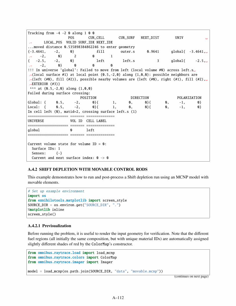
Tracking from -4 -2 0 along 1 0 0POS CUR_CELL CUR_SURF NEXT_DIST UNIV
→ LOCAL_POS VOLID SURF_IDX NEXT_IDX...moved distance 0.535898384862246 to enter geometry-3.4641, -2, 0 fill outer.s 0.9641 global -3.4641,→ -2, 0 2 0 1 -2.5, -2, 0 left left.s 3 global -2.5,→ -2, 0 0 0 0!!! In universe 'global': Failed to move from left (local volume #0) across left.s→(local surface #1) at local point 0.5,-2,0 along 1,0,0: possible neighbors are→left (#0), fill (#2), possible nearby volumes are left (#0), right (#1), fill (#2),→EXTERIOR (#3)^^^ at 0.5,-2,0 along 1,0,0Failed during surface crossing:
POSITION DIRECTION POLARIZATIONGlobal: 0.5, -2, 0 1, 0, 0 0, -1, 0Local: 0.5, -2, 0 1, 0, 0 0, -1, 0In cell left (0), matid=2, crossing surface left.s (1)==================== ======= ==============UNIVERSE VOL ID CELL LABEL==================== ======= ==============global 0 left==================== ======= ==============
Current volume state for volume ID = 0:Surface IDs: 1Senses: -Current and next surface index: 0 -> 0
A.4.2 SHIFT DEPLETION WITH MOVABLE CONTROL RODS
This example demonstrates how to run and post-process a Shift depletion run using an MCNP model withmovable elements.
# Set up example environmentimport osfrom exnihilotools.matplotlib import screen_styleSOURCE_DIR = os.environ.get("SOURCE_DIR", ".")%matplotlib inlinescreen_style()
A.4.2.1 Previsualization
Before running the problem, it is useful to render the input geometry for verification. Note that the differentfuel regions (all initially the same composition, but with unique material IDs) are automatically assignedslightly different shades of red by the ColorMap’s constructor.
from omnibus.raytrace.load import load_mcnpfrom omnibus.raytrace.colors import ColorMapfrom omnibus.raytrace.imager import Imager
model = load_mcnp(os.path.join(SOURCE_DIR, "data", "movable.mcnp"))
(continues on next page)
A–112

(continued from previous page)
colors = ColorMap.from_compositions(model.compositions)colors[colors.unassigned] = 'Set3'imager = Imager(model.geometry,
lower=(-20, 0, -20),upper=(20, 0, 20),basis=(1, 0, 0),max_pixels=1024)
imager.names = [c.name for c in model.compositions]imager.colors = colorsimager.plot();
Generating MCNP runtpe file......finished generating MCNP runtpe file in 2.8 seconds
The model’s composition data can be used to plot number densities in the reactor. The first step in such avisualization is extracting number densities and their corresponding nuclide IDs from the model’s composi-tions. Note that zaid returns a view (which for efficiency we translate into a numpy array), whereas calc_ndreturns a vector that is automatically translated to a native python object.
import numpy as np
def calc_number_densities(comp):return dict(zip(np.asarray(comp.zaid).tolist(), comp.calc_nd()))
def calc_mass_densities(comp):zaid = np.asarray(comp.zaid)wt = np.asarray(comp.get_wt_fractions()) * comp.densityreturn dict(zip(zaid.tolist(), wt.tolist()))
(continues on next page)
A–113

(continued from previous page)
densities = [calc_mass_densities(c) for c in model.compositions]densities[10]
1001: 0.06633015932148201,8016: 0.5422080954790859,92235: 9.085977478992715,92238: 0.6606715344205284
The next step is to extract a particular nuclide’s densities for every pixel’s matid in the raytrace’s view. Thisrequires a Numpy array of values for each matid. Using np.nan instead of 0.0 means the value will be hiddenrather than rendered as a zero-value, making it more obvious which parts of the problem have trace nuclidesas opposed to none of the nuclide. The pcolor method of the Imager will render an image where the valueof each pixel is calculated from the index in the pcolor argument vector corresponding to the material ID atthat pixel.
def get_dens(zaid):return np.array([d.get(zaid, np.nan) for d in densities])
u235 = get_dens(92235)assert u235[10] == densities[10][92235]assert np.isnan(u235[0])
imager.pcolor(u235);
Here is the mass density plot for hydrogen:
A–114

imager.pcolor(get_dens(1001));
With a little code, it is possible to automate the rendering of all the nuclides in the problem:
from matplotlib.colors import LogNormfrom matplotlib.offsetbox import AnchoredTextimport matplotlib.pyplot as pltfrom omnibus.db.validator import to_nuclide
zaids = set()for d in densities:
zaids.update(d.keys())
zaid_to_nuclide = to_nuclide.zaid_to_pretty_nuclidenorm = LogNorm(vmin=0.05, vmax=10.0)
nr = int(np.ceil(np.sqrt(len(zaids))))fig, axes = plt.subplots(nr, nr, figsize=(9,9))
ijax_iter = np.ndenumerate(axes)for (zaid, ((i,j), ax)) in zip(sorted(zaids), ijax_iter):
show_colorbar = (i == 0 and j == 0)
# Plot the actual densitiesimager.pcolor(get_dens(zaid), ax=ax, colorbar=show_colorbar, norm=norm)
# Add a nice inset titleat = AnchoredText(zaid_to_nuclide(zaid),
prop=dict(size=8), frameon=True,loc=2)
(continues on next page)
A–115
(continued from previous page)
at.patch.set_boxstyle("round,pad=0.,rounding_size=0.2")ax.add_artist(at)
# Hide tick labels if it's not the outermost plot on the upper leftif i == 0:
ax.xaxis.set_label_position('top')ax.xaxis.set_ticks_position('top')
else:ax.set_xlabel("")ax.set_xticklabels([])
if j != 0:ax.set_ylabel("")ax.set_yticklabels([])
# Clear remaining axesfor ((i,j), ax) in ijax_iter:
fig.delaxes(ax)
/usr/local/anaconda3/envs/exnihilo/lib/python3.7/site-packages/matplotlib/colors.→py:1028: RuntimeWarning: invalid value encountered in less_equalmask |= resdat <= 0
A–116

A.4.2.2 Execute Omnibus
The following Omnibus depletion input transports on this model with four kcode solves, using alternatingburn/decay steps. Before the first step, the control rod is moved downward by 10 cm; the next time step it ismoved upward by 5 cm.
%cat SOURCE_DIR/data/movable.omn!omnibus-run SOURCE_DIR/data/movable.omn
[PROBLEM]name "Depletion problem with moving control rod"mode kcode
[MODEL=mcnp]input "movable.mcnp"
(continues on next page)
A–117

(continued from previous page)
extents -100 100 -100 100 -100 100
[MODEL][MOVABLE=surfaces control_rod]surfaces 1 2
[DEPLETION]deplete_cells 201 202 203
211 212 213221 222 223
tracking_set "addnux1" ! TRITON "addnux" settracking_nuclides na-23 ! additional nuclides to track! Decay stepsburn_length : decay_length : power : num_burn_steps : num_decay_steps
1.0 1.0 0.005 1 11.5 0.7 0.005 1 1
! Write cross sections to HDF5write_xs true! Reduce accuracy but reduce run timepredictor_substeps 1renormalization_method boss
[DEPLETION][MOVE control_rod]! movement for each time step: -20 is fully inserted, 0 is fully outdelta -10.0 5.0
[PHYSICS=ce]ce_lib ce_v71mode n
[SOURCE=separable fission][SOURCE][SHAPE=box]box -3.25 3.25 -3.25 3.25 -9.0 9.0
[SHIFT]
[.][KCODE]num_histories_per_cycle 1000num_cycles 20num_inactive_cycles 5
[TALLY][.][CYLMESH globalcyl]reactions flux nu_fissionr 0 4.33012702 6.12372436 7.5 9.5 12 20 50theta 0 3i 1.0z -20 -15 -9 5i 9 15 20
[..][CELL fuel]reactions flux nu_fissioncells 201 202 203
211 212 213221 222 223
(continues on next page)
A–118

(continued from previous page)
nbins 1e7 39ilog 1e-3
[RUN=mpi]np 4INFO: Starting Omnibus preprocessor, omnibus version 6.3.pre-b10 (branch 'omnibus-doc'→#98d73c8e on 2020MAR11)Loading problem db from Omnibus ASCII file...Loading Omnibus input file at /rnsdhpc/code/src/scale/Exnihilo/packages/Omnibus/driver/→example/data/movable.omn
...finished loading problem db from Omnibus ASCII fileLoading problem db from Python file...
...finished loading problem db from Python fileINFO: Set default for 'mpiexec_args' to '['-np', '4']' in '/run'Generating MCNP runtpe file...
...finished generating MCNP runtpe fileINFO: Set default for 'energy' to ''_type': 'watt'' in '/source/fission'INFO: Defaulting Watt spectrum to U-235INFO: Set default for 'angle' to ''_type': 'isotropic'' in '/source/fission'INFO: Set default for 'fissionable_only' to 'True' in '/source/fission'INFO: Set default for 'xs_cache' to 'totfisnu' in '/physics/ce'INFO: Set default for 'xs_accel' to 'True' in '/physics/ce'INFO: Set default for 'fission_neutrons' to 'False' in '/physics/ce/fission'INFO: Set default for 'load_scl' to 'True' in '/comp'INFO: Set default for 'decomposition' to ''_type': 'none'' in '/shift'INFO: Set default for 'verbosity' to 'none' in '/shift/transporter'INFO: Set default for 'method' to 'roulette' in '/shift/vr'INFO: Writing Omnibus input ParameterList to movable.inp.xmlINFO: Writing preprocessed file to movable.pp.jsonINFO: Writing processed ASCII input to 'movable.inp.omn'INFO: Launching Omnibus driver on 4 coresRunning Omnibus...WARNING: The Exnihilo software revision (r540) used to generate the input file differs→from this version being used to run it (r539).WARNING: This could cause internal consistency checks to unexpectedly fail, and it could→even lead to unexpected database value changes.WARNING: Please check your output very carefully after this run to make sure the→interpreted values match your input values.Building modelINFO: Loading SCALE Standard Composition Library from /usr/local/scale/data/scale.rev40.→sclibINFO: Loading compositions from MCNP inputINFO: Creating default boundary mesh from (-100 -100 -100) to (100 100 100) for MCNP→geometryBuilding physics 'ce'INFO: Loading CE library /usr/local/scale/hpcdata/ce_v7.1_endf.h5INFO: Corrected thermal xs balance: 1.2e-05% error in h-1 @ 293.6KBuilding talliesBuilding sourcesBuilding Shift solver internalsBuilding Shift sourcesInitializing Shift solverBuilding depletion solver internals
(continues on next page)
A–119

(continued from previous page)
INFO: Using the default VESTA group structure in the depletion tallyBuilding depletion material dataINFO: Loading ORIGEN library /usr/local/scale/data/origen_library/pwr.rev03.orglibINFO: Loading fission yield library /usr/local/scale/data/origen_data/origen.rev05.yields.→dataINFO: Loading JEFF multigroup library /usr/local/scale/data/origen.rev01.jeff252gLoading depletion cross sectionsINFO: Total initial heavy-metal mass in system: 0.0310027 MTBuilding Shift talliesSolving depletion step 0 from 0 days to 1 days at 0.005 MWINFO: Moving control_rod by -10 cmRunning Shift transport calculationBeginning inactive cyclesINFO: Completed 5 inactive cyclesBeginning active cyclesINFO: Completed 15 active cyclesCollapsing cross sectionsWriting tally resultsSolving depletion step 1 from 1 days to 2 days at 0 MWINFO: Deleted delayed fission data because the CE data lacks a delayed fission spectrum:→cm-243 @ 293K, am-242m @ 293KRunning Shift transport calculationBeginning inactive cyclesINFO: Completed 5 inactive cyclesBeginning active cyclesINFO: Completed 15 active cyclesCollapsing cross sectionsWriting tally resultsSolving depletion step 2 from 2 days to 3.5 days at 0.005 MWINFO: Moving control_rod by 5 cmRunning Shift transport calculationBeginning inactive cyclesINFO: Completed 5 inactive cyclesBeginning active cyclesINFO: Completed 15 active cyclesCollapsing cross sectionsWriting tally resultsSolving depletion step 3 from 3.5 days to 4.2 days at 0 MWRunning Shift transport calculationBeginning inactive cyclesINFO: Completed 5 inactive cyclesBeginning active cyclesINFO: Completed 15 active cyclesCollapsing cross sectionsWriting tally resultsRunning Shift transport calculationBeginning inactive cyclesINFO: Completed 5 inactive cyclesBeginning active cyclesINFO: Completed 15 active cyclesCollapsing cross sectionsWriting tally results
(continues on next page)
A–120

(continued from previous page)
WARNING: The first and second halves of the active cycles have statistically different (3.→75514 sigma) Shannon entropyRun completeCleaning up
...finished running Omnibus in 11.2 secondsRunning Omnibus postprocessingLoading HDF5 file...INFO: Loaded Omnibus output data from 'movable.out.h5', problem name 'Depletion problem→with moving control rod', created on 2020MAR11 22:38 using SCALE version 6.3.pre-b10→(branch 'omnibus-doc' #17579cc6 on 2020MAR10)
...finished loading HDF5 fileLoading HDF5 file...INFO: Loaded Omnibus output data from 'movable.out.h5', problem name 'Depletion problem→with moving control rod', created on 2020MAR11 22:38 using SCALE version 6.3.pre-b10→(branch 'omnibus-doc' #17579cc6 on 2020MAR10)
...finished loading HDF5 filePlotting k-effective and related diagnostics.../rnsdhpc/code/build/Exnihilo-examples/Exnihilo/packages/Omnibus/python/omnibus/formats/→tally/field.py:308: FutureWarning: Using a non-tuple sequence for multidimensional→indexing is deprecated; use `arr[tuple(seq)]` instead of `arr[seq]`. In the future→this will be interpreted as an array index, `arr[np.array(seq)]`, which will result→either in an error or a different result.mom = data[slc]
INFO: Saved k-eff plot to movable.keff.pdf...finished plotting k-effective and related diagnostics in 1.4 seconds
Writing cell tally results to CSV files...INFO: Wrote cell tally 'fuel' to movable.fuel.t0.csvINFO: Wrote cell tally 'fuel' to movable.fuel.t1.csvINFO: Wrote cell tally 'fuel' to movable.fuel.t2.csvINFO: Wrote cell tally 'fuel' to movable.fuel.t3.csvINFO: Wrote cell tally 'fuel' to movable.fuel.t4.csv
...finished writing cell tally results to CSV filesWriting mesh tally visualization file...
...finished writing mesh tally visualization fileWriting depletion number densities...INFO: Not creating number density CSV file because it would be too large (expected size→1289 kB exceeds user-given size 4000000); set the 'csv_max' parameter or use Python→tools
...finished writing depletion number densitiesWriting depletion cross sections...Writing cross sections to CSV...
...finished writing cross sections to CSVINFO: Wrote depletion cross sections to movable.xs.csv
...finished writing depletion cross sectionsBuilding RST summary...INFO: Wrote summary file to movable.rst
...finished building RST summary
The output file produced includes all the data from the run: debug information, system information, logmessages, etc.
A–121

from omnibus.formats.output import loadoutput = load("movable.out.h5")output
Loading HDF5 file...INFO: Loaded Omnibus output data from 'movable.out.h5', problem name 'Depletion problem→with moving control rod', created on 2020MAR11 22:38 using SCALE version 6.3.pre-b10→(branch 'omnibus-doc' #17579cc6 on 2020MAR10)
...finished loading HDF5 file
For example, the compositions can be extracted and printed (only a subset is shown here, for brevity):
output['comp']['compositions'].tolist()[1:3]
['matid': 1,'name': 'm20','temperature': 293.59433519120626,'density': 2.688233813164135,'fissionable': False,'depletable': False,'zaid': array([13027], dtype=uint32),'wtfrac': array([1.]),
'matid': 2,'name': 'm30','temperature': 293.59433519120626,'density': 4.180967304626936,'fissionable': False,'depletable': False,'zaid': array([ 8016, 13027, 63151, 63153], dtype=uint32),'wtfrac': array([0.0784097 , 0.42199784, 0.23721664, 0.26237582])]
The following block of code extracts all the output groups that correspond to an Omnibus run sequence, andthen sorts them by their execution order (the index accessor).
memory = [(name, block['peak_memory'].data['global'])for (name, block) in output.items() if 'peak_memory' in block]
memory.sort(key=(lambda n_pm: output[n_pm[0]].index))memory
[('system', 223484),('model', 315388),('comp', 315552),('physics-ce', 780108),('tally', 1669588),('source', 781292),('depletion', 1668844),('shift', 1821808)]
The ‘tally’ memory usage is higher than the ‘source’ usage due to an internal implementation detail. (Thetallies are initialized before the source but saved after the depletion tallies have been created.)
A–122
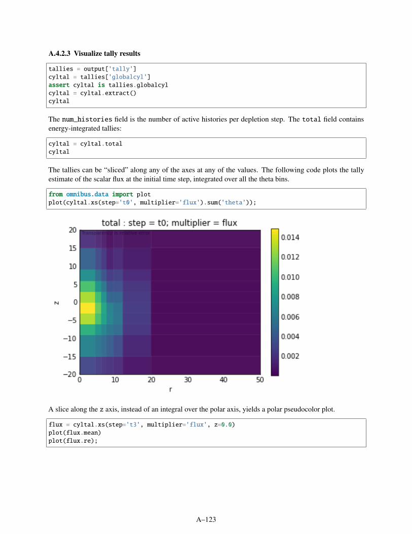
A.4.2.3 Visualize tally results
tallies = output['tally']cyltal = tallies['globalcyl']assert cyltal is tallies.globalcylcyltal = cyltal.extract()cyltal
The num_histories field is the number of active histories per depletion step. The total field containsenergy-integrated tallies:
cyltal = cyltal.totalcyltal
The tallies can be “sliced” along any of the axes at any of the values. The following code plots the tallyestimate of the scalar flux at the initial time step, integrated over all the theta bins.
from omnibus.data import plotplot(cyltal.xs(step='t0', multiplier='flux').sum('theta'));
A slice along the z axis, instead of an integral over the polar axis, yields a polar pseudocolor plot.
flux = cyltal.xs(step='t3', multiplier='flux', z=0.0)plot(flux.mean)plot(flux.re);
A–123

Cell tallies can also be plotted:
celltal = tallies['fuel'].extract()binned_tally = celltal['binned']print(binned_tally.mesh('cell'))binned_tally
A–124

['201' '202' '203' '211' '212' '213' '221' '222' '223']
plot(binned_tally.xs(step='t0', multiplier='flux', stat='mean', cell='213'),logy=True);
From the spectrum, this is clearly a fast reactor.
In conjunction with the Imager, cell tally results can actually be rendered onto the geometry with a ray trace.Here is a slice of the cells in the geometry at y = 0:
imager = Imager(model.geometry,lower=(-20, 0, -20),upper=(20, 0, 20),basis=(1, 0, 0),max_pixels=1024,trace='cell')
imager.plot();
A–125

Plotting the reaction rates in each cell requires one-dimensional data (one value per cell), so here are theenergy-integrated fluxes at one particular time step.
cell_production = celltal.total.xs(step='t3', stat='mean', multiplier='nu_fission')print(cell_production.selection)print("Active dimensions:", cell_production.dims)imager.pcolor(cell_production.data, labels=cell_production.mesh('cell'));
step = t3; multiplier = nu_fission; stat = meanActive dimensions: ['cell']
A–126

A.4.2.4 Visualize depletion results
Additional processing and visualization can be peformed from the number densities and one-group crosssections in the depletion output.
# Reduce number of output rows to keep the documentation smallimport pandas as pdpd.options.display.max_rows = 15
depl = output['depletion']depl
The number density is a function of step, cell, and ZAID. Note that to support restart capability, the“zaid” axis has duplicate entries in it, since ORIGEN tracks some nuclides multiple times. A built-incollapse_nuclides function consolidates these nuclides. Calling this function on a field will pull theentire dataset from disk and return a new field with the collapsed nuclides. This is going to be memory-,disk-, and CPU-intensive, so it is not a bad idea to slice the data first to reduce the amount of work that has tobe done if the entire result is not needed.
num_dens = depl.num_densnum_dens
num_dens = num_dens.collapse_nuclides()num_dens
Note that the data entry of the initial num_dens points to an on-disk HDF5 object, whereas after collapsingnuclides the data is an in-memory Numpy array.
A–127

# Convert xenon densities to a Pandas dataframexe_dens = num_dens.xs(zaid=to_nuclide('xe-135')).to_series().unstack('cell')xe_dens
/rnsdhpc/code/build/Exnihilo-examples/Exnihilo/packages/Omnibus/python/omnibus/data/field.→py:692: FutureWarning: the 'labels' keyword is deprecated, use 'codes' insteadindex = pd.MultiIndex(levels=levels, labels=labels, names=names)
# Change indexing from labels to actual simulated timesimtime = depl.simtime.extract()xe_dens.index = simtime.data
# Plot number densities in each cellax = xe_dens.plot(marker='x')ax.set_ylabel("Xe-135 density ()".format(num_dens.units))ax.set_xlabel("Time ()".format(simtime.units))
# Plot powerpower = depl.totpower.extract()ax2 = ax.twinx()ax2.plot(simtime.data, power.data, drawstyle='steps-post', linewidth=2, color=(0,0,0,.5))ax2.set_ylabel("Power ()".format(power.units))
Text(0, 0.5, 'Power (MW)')
The collapsed cross sections are stored in a single array that holds (ZAID,MT) pairs (since not all nuclideshave all reaction types). Because the omnibus.data.Field class is built for only regular multi-dimensionaldata (no ragged edges), it can be easier to process this field using the Pandas package. The to_series
A–128

function converts a field into a Pandas series. The zaid_mt axis gets expanded into two different “levels” ina pandas.MultiIndex object.
# Print a table of cross sections, with step/zaid/mt as rowsxs = depl['xs'].to_series().unstack('cell')xs
/rnsdhpc/code/build/Exnihilo-examples/Exnihilo/packages/Omnibus/python/omnibus/data/field.→py:652: FutureWarning: .labels was deprecated in version 0.24.0. Use .codes instead.lab[:] = list(zip(*mi.labels))
# Tabulate just the fission cross sections_.xs(18, level='mt')
# View U-235 cross sections as a function of time in each of the different cells_.xs(92235, level='zaid').plot();
A.4.3 CUSTOM COMPOSITIONS IN OMNIBUS
The Omnibus [COMP][MATERIAL] block is convenient for defining small numbers of compositions with fewnuclides, but it can be tedious to use for more complex inputs, and especially tedious if the compositions arealready defined in another input model. This example demonstrates how to extract compositions from anexisting SCALE input and use them in an Omnibus problem with a Geometria-based geometry.
# Set up example environmentimport osfrom exnihilotools.matplotlib import screen_styleSOURCE_DIR = os.environ.get("SOURCE_DIR", ".")%matplotlib inline
(continues on next page)
A–129
(continued from previous page)
%load_ext wurlitzerscreen_style()
A.4.3.1 Load existing compositions
Loading the SCALE model provides access to both the geometry definition and the compositions. The_asdict method of a composition object allows it to be rendered as a native Python dictionary for easyperusal.
from omnibus.raytrace.load import load_scalescale_model = load_scale(os.path.join(SOURCE_DIR, "data", "godiva-keno.inp"))comps = [c._asdict() for c in scale_model.compositions]comps
>>> Using SCALE geometry from 'csas6' sequence.>>> Loading SCALE Standard Composition Library from /usr/local/scale/data/scale.rev40.→sclib
['name': 'void','matid': 0,'temperature': 1e-07,'density': 0.0,'fissionable': False,'depletable': False,'zaid': array([], dtype=uint32),'wtfrac': array([], dtype=float64),
'name': 'media 1','matid': 1,'temperature': 293.0,'density': 18.739884256874777,'fissionable': True,'depletable': True,'zaid': array([92234, 92235, 92238], dtype=uint32),'wtfrac': array([0.01019995, 0.93709968, 0.05270038])]
A.4.3.2 Exporting compositions
The compositions can be immediately saved to disk if they do not need modification:
from robus import save_hdf5_compositionssave_hdf5_compositions("godiva_keno.comp.h5", scale_model.compositions)
Changing the names and ordering of the compositions demonstrate some of the capabilities of the Pythonrepresentation of the compositions. Writing Python objects to HDF5 requires the Omnibus format wrappers(usually seen when processing existing Omnibus output files).
import h5pyfrom omnibus.data import dump_rootfrom omnibus.formats.comp import Compositions, CompBlock
(continues on next page)
A–130

(continued from previous page)
# Create a compositions object with modified propertiescomps[1]['name'] = 'uranium'comps = [comps[1], comps[0]]
# TODO: this may not be necessary for Omnibus, but it currently is necessary for→raytracingfor matid, c in enumerate(comps):
c['matid'] = matid
export_comps = Compositions.from_list(comps)export_comp_block = CompBlock(data='compositions': export_comps)with h5py.File(os.path.join(SOURCE_DIR, "data", "godiva-gg.comps.h5"), 'w') as f:
dump_root(export_comp_block, f)
A.4.3.3 Using compositions with GG
Now that updated compositions have been computed, they can be loaded as part of the Geometria modelfor raytracing. Although this example uses compositions loaded directly from a SCALE model, it is alsopossible to directly use compositions loaded from an existing Omnibus HDF5 output file, in which caseexport_comps here would be replaced by output_file['comp']['compositions'].
from omnibus.raytrace.load import load_ggmodel = load_gg(os.path.join(SOURCE_DIR, "data", "godiva.gg.omn"),
compositions=export_comps)
Generating Geometria XML input file from .gg.omn...INFO: Starting Geometria preprocessor, omnibus version 6.3.pre-b11 (branch 'comp-example→' #4d164aa1 on 2020APR14)Loading problem db from Omnibus ASCII file...Loading Omnibus input file at /rnsdhpc/code/src/scale/Exnihilo/packages/Omnibus/driver/→example/data/godiva.gg.omn
...finished loading problem db from Omnibus ASCII fileINFO: Writing Geometria input ParameterList to godiva.gg.xml
...finished generating Geometria XML input file from .gg.omn
from omnibus.raytrace.colors import ColorMapfrom omnibus.raytrace.imager import Imager
colors = ColorMap.from_compositions(model.compositions)imager = Imager.from_extents(model.geometry, z=0.0)imager.names = [c.name for c in model.compositions]imager.colors = colorsimager.plot();
A–131

A.5 CE DATA
A.5.1 INTERACTING WITH CE CROSS SECTION DATA
This example demonstrates some basic tools for interacting with AMPX-processed continuous energy crosssections.
# Set up example%matplotlib inlinefrom exnihilotools.matplotlib import screen_style, gridscreen_style()
Providing various options to the Library loader, such as disabling the loading of kinematics data, will reducedata load times and memory consumption. Printing the database after loading shows the defaults for otheroptions not provided in the input database.
from nemesis import cmake_config, Std_DB, make_view, make_const_viewfrom robus import Libraryfrom omnibus.db.validator import mt_to_str, to_mt, to_nuclidefrom omnibus.scale import ce_file_resolver
db = Std_DB.from_dict('ce_lib_path': ce_file_resolver.resolve("ce_v7.1_endf"),'gamma_production': False,'kinematics': False,'reactions': [to_mt(k) for k in """N_TOTAL N_ELASTIC N_FISSION N_ABSORPTION
N_N_X1 N_N_XC N_GAMMA N_NU N_SAB""".split()],'broaden_db':
'kinematics': False,
(continues on next page)
A–132

(continued from previous page)
)library = Library(db)print(db)
/rnsdhpc/code/install/Exnihilo/python/omnibus/__init__.py:93: UserWarning: Version→mismatch between 'exnihilotools' and 'omnibus' packages: 6.3.pre-b10 (branch 'omnibus-→doc' #98d73c8e on 2020MAR11) (at /rnsdhpc/code/build/Exnihilo-examples/Exnihilo/→packages/Nemesis/python/exnihilotools/__init__.py) is not the same as 6.3.pre-b10→(branch 'fix-origen-install' #b3af8ef1 on 2020MAR06) (at /rnsdhpc/code/install/Exnihilo/→python/omnibus/__init__.py); This is probably because of a PYTHONPATH error and may→cause unexpected failures on importUserWarning)
############################################################Path: /std_db
Database for std_db has:2 integer entries5 double entries9 bool entries1 string entries7 vector<int> entries0 vector<double> entries0 vector<string> entries0 vector<bool> entries1 nested database entries
============================================================Entries in std_db database============================================================integer entries------------------------------------------------------------
sizeof_data_float 4sizeof_energy_float 8
double entries------------------------------------------------------------
ethermal 10n_energy_max 2e+07n_energy_min 1e-05p_energy_max 2.5e+07p_energy_min 10000
bool entries------------------------------------------------------------
collision_moments 0collision_pdf 0
collision_probabilities 0dbrc 1
gamma_production 0kinematics 0
(continues on next page)
A–133

(continued from previous page)
missing_as_zero 0probability_tables 1
unionize_energy 0
string entries------------------------------------------------------------
ce_lib_path/usr/local/scale/hpcdata/ce_v7.1_endf.h5
vector<int> entries (number of elements)------------------------------------------------------------
omit_zaid_n 0omit_zaid_p 0orig_zaid_n 0orig_zaid_p 0reactions 9
subs_zaid_n 0subs_zaid_p 0
############################################################Path: /std_db/broaden_db
Database for broaden_db has:0 integer entries1 double entries2 bool entries0 string entries0 vector<int> entries0 vector<double> entries0 vector<string> entries0 vector<bool> entries0 nested database entries
============================================================Entries in broaden_db database============================================================double entries------------------------------------------------------------
temperature_tol 4
bool entries------------------------------------------------------------
kinematics 0legacy 0
########################################################################################################################
A.5.1.1 Analyze energy grid spacing
How are the energy grid points distributed for water-bound hydrogen? The Exnihilo python bindings canextract any property of the physics data and manipulate it natively in Python. Here, the ubiquitous Numpypackage’s powerful math utilities are used to plot a distribution of the relative spacing of the energy grid
A–134

points.
import numpy as npimport matplotlib.pyplot as plt
def centers(x):return (x[:-1] + x[1:]) * 0.5
nucl = library.load_nuclide_n(1001, 293)rxn = nucl.get_reaction(to_mt("N_TOTAL"))energy = np.asarray(rxn.energy)
delta_e = np.diff(energy)energy_mid = centers(energy)relative_delta_e = delta_e
(fig, ax) = plt.subplots(subplot_kw=dict(xscale='log', yscale='log'))ax.hist(relative_delta_e, bins=np.logspace(-15,0,31));grid(ax, 'both')
Plotting as a function of energy reveals that the thermal range has lots of micro-sized points, likely a result ofAMPX processing of the thermal scattering.
def plot_rel_spacing(energy_mid, delta_e):(fig, ax) = plt.subplots(subplot_kw=dict(xscale='log', yscale='log'))ax.plot(energy_mid, delta_e/energy_mid, linestyle='none', marker='.')ax.set_xlabel("Energy [eV]")ax.set_ylabel("Relative spacing of grid points")grid(ax, which='major')return ax
plot_rel_spacing(energy_mid, delta_e);
A–135

Comparing against free-gas hydrogen confirms that the artifacts are related to the bound cross sectiontreatment:
nucl = library.load_nuclide_n(8001001, 293)rxn = nucl.get_reaction(to_mt("N_TOTAL"))energy = np.asarray(rxn.energy)
ax = plot_rel_spacing(centers(energy), np.diff(energy))ax.set_ylim(1e-15, 1);
A–136

A.5.1.2 Resonance broadening
This example shows how Doppler broadening affects the cross sections of a large iron resonance. Thebroaden_db option passed to the Library above enables run-time broadening of cross sections, even if notpreviously generated for the CE library being used.
zaid = to_nuclide('Fe-56')print("Nuclide ID: ", zaid)rxn_mt = to_mt("N_TOTAL")print("Reaction MT:", mt_to_str(rxn_mt))
# Pre-load temperatures, including interpolated at midpointtemperatures = sorted(set(library.get_temperatures(zaid)) | 420, 750, 900, 1800)library.load_nuclide_n(zaid, temperatures)
nuclides = [library.load_nuclide_n(zaid, t) for t in temperatures]print("Loaded temperatures: " + ", ".join(str(nucl.temperature) for nucl in nuclides))
Nuclide ID: 26056Reaction MT: 1=N_TOTALLoaded temperatures: 293.0, 420.0, 565.0, 600.0, 750.0, 900.0, 1200.0, 1800.0, 2000.0,→2400.0
Plot an overall view of the cross sections:
nucl = nuclides[0]rxn = nucl.get_reaction(rxn_mt)
def get_desc(nucl, rxn):return ":s at :.1f for MT :s".format(
(continues on next page)
A–137

(continued from previous page)
to_nuclide.zaid_to_pretty_nuclide(nucl.zaid),nucl.temperature,to_mt.to_str(rxn.mt))
(fig, ax) = plt.subplots()ax.loglog(rxn.energy, rxn.xs, '-')ax.set_title(get_desc(nucl, rxn))grid(ax)
A close-up visualization of the lowest-energy resonance shows how the cross sections vary as a function oftemperature:
from matplotlib.cm import get_cmapfrom matplotlib.colors import LogNormcmap = get_cmap('coolwarm')norm = LogNorm(vmin=nuclides[0].temperature, vmax=nuclides[-1].temperature)
(fig, ax) = plt.subplots()ax.set_xlim(1140, 1160)ax.set_ylim(0, 100)for nucl in nuclides:
rxn = nucl.get_reaction(rxn_mt)plt.plot(rxn.energy, rxn.xs,'-o',
markeredgecolor="none", markersize=2,label=":.1f".format(nucl.temperature),color=cmap(norm(nucl.temperature)))
ax.legend(loc="upper right")grid(ax)
A–138

The values at the cross sections at the peaks of these resonances can be found using Numpy:
for nucl in nuclides:rxn = nucl.get_reaction(rxn_mt)e = np.asarray(rxn.energy)xs = np.asarray(rxn.xs)erange = (e > 1100) & (e < 1200)max_local_index = np.argmax(xs[erange])max_index = np.where(erange)[0][max_local_index]print("For :s at :7.1f, resonance peaks at index :d "
"(E = :.3f eV) with sigma = :.1f cm^-1".format(to_nuclide.zaid_to_pretty_nuclide(nucl.zaid),nucl.temperature, max_index, e[max_index], xs[max_index]))
For Fe-56 at 293.0, resonance peaks at index 613 (E = 1149.700 eV) with sigma = 79.4→cm^-1For Fe-56 at 420.0, resonance peaks at index 436 (E = 1149.748 eV) with sigma = 70.0→cm^-1For Fe-56 at 565.0, resonance peaks at index 612 (E = 1149.700 eV) with sigma = 62.9→cm^-1For Fe-56 at 600.0, resonance peaks at index 612 (E = 1149.700 eV) with sigma = 61.6→cm^-1For Fe-56 at 750.0, resonance peaks at index 436 (E = 1149.748 eV) with sigma = 56.8→cm^-1For Fe-56 at 900.0, resonance peaks at index 606 (E = 1149.700 eV) with sigma = 53.2→cm^-1For Fe-56 at 1200.0, resonance peaks at index 606 (E = 1149.700 eV) with sigma = 47.9→cm^-1For Fe-56 at 1800.0, resonance peaks at index 436 (E = 1149.748 eV) with sigma = 41.6→cm^-1For Fe-56 at 2000.0, resonance peaks at index 614 (E = 1149.597 eV) with sigma = 39.9→cm^-1
(continues on next page)
A–139

(continued from previous page)
For Fe-56 at 2400.0, resonance peaks at index 617 (E = 1149.597 eV) with sigma = 37.5→cm^-1
A.5.1.3 Cross section interpolation
The Python methods in this notebook directly access the underlying Shift C++ data using Numpy arrays,with no copying, enabling high performance (speed of C rather than Python) operations on large data sets.This example demonstrates the performance of interpolating the hydrogen cross section onto a 100k-pointenergy grid.
nucl = library.load_nuclide_n(1001, 600.0)rxn = nucl.get_reaction(1)print("Reaction: MT :s from :s at :.1fK".format(
to_mt.to_str(rxn.mt),to_nuclide.zaid_to_pretty_nuclide(nucl.zaid),nucl.temperature,))
from physica import calc_micro_xsinterp_energy = np.logspace(-3, 6, 100000)interp_xs = np.zeros_like(interp_energy, dtype='float32')print("Interpolation time:")%timeit calc_micro_xs(rxn, make_const_view(interp_energy), make_view(interp_xs))
Reaction: MT 1=N_TOTAL from H-1 at 600.0KInterpolation time:1.24 ms ? 19.5 ?s per loop (mean ? std. dev. of 7 runs, 1000 loops each)
A.5.1.4 Find nonlinear interpolation schemes
Most of the SCALE cross sections use linear-linear interpolation. To check whether any nonlinear interpola-tion is used at all, one can loop through all reactions in all nuclides. To reduce load time, gamma productiondata and kinematics (collision) data are ignored.
from robus import NEUTRON
library = Library(Std_DB.from_dict('ce_lib_path': ce_file_resolver.resolve("ce_v71"),'gamma_production': False,'kinematics': False,'probability_tables': False
))
for zaid in library.get_zaids(NEUTRON):temperature = 300.nucl = library.load_nuclide_n(zaid, temperature)for mt in nucl.get_mts():
rxn = nucl.get_reaction(mt)if rxn.find_interpolation(0) != 2:
print(zaid, mt)
A–140

88223 45288226 452
The two nonlinear interpolations are for nu (average neutron yield per fission) in two isotopes of radium!
(fig, axes) = plt.subplots(2, 2, figsize=(8,8))
for (i, zaid) in enumerate([88223, 88226]):nucl = library.load_nuclide_n(zaid, 293)for (j, mt) in enumerate([452, 18]):
ax = axes[i, j]rxn = nucl.get_reaction(mt)ax.loglog(rxn.energy, rxn.xs, '-o',
markeredgecolor="none", markersize=3)ax.set_title(get_desc(nucl, rxn))ax.set_xlabel("E [eV]")ax.set_ylabel("$\sigma$")
plt.tight_layout()
A–141

It is exceedingly odd that Radium has fission and production reactions, and that its fission reaction has thatobviously nonphysical shape. This has the smell of bad ENDF data.
A.5.1.5 Debug errors during broadening
During testing of a new feature, Shift developers discovered that the highest few energy grid points in Fe-56were being broadened strangely, producing large relative errors. Additionally, broadening of MT=5 failed.This section shows some of the steps taken to debug the failure.
db = Std_DB.from_dict('ce_lib_path': ce_file_resolver.resolve("ce_v71"),'gamma_production': False,'kinematics': False,
(continues on next page)
A–142

(continued from previous page)
)library = Library(db)nucl = library.load_nuclide_n(26056, 300.0)rxn = nucl.get_reaction(1)
The cross sections for the highest energies are plotted here:
(fig, ax) = plt.subplots()ax.plot(rxn.energy, rxn.xs,'-o',
markeredgecolor="none", markersize=4,)
(energy, xs) = (np.asarray(v) for v in (rxn.energy, rxn.xs))ax.set_xlim(energy[-5], 2 * energy[-1] - energy[-5])ax.set_ylim(.8 * xs[-1], 1.2 * xs[-1])ax.set_title(get_desc(nucl, rxn))ax.grid();
print("Final energy points:", energy[-5:])
Final energy points: [19999508.63125662 19999749.43095107 19999754.31487379 20000000.20000010. ]
Note that the discontinous point at the end of the cross section is above the maximum requested energy,indicating an error in the CE data processing.
Next let’s look at MT 5, which was crashing because it had fewer than ~6 energy grid points.
A–143

rxn = nucl.get_reaction(5)print("Energy:", np.asarray(rxn.energy))print("XS: ", np.asarray(rxn.xs))
(fig, ax) = plt.subplots()ax.semilogx(rxn.energy, rxn.xs, 'b-x')ax.set_title(get_desc(nucl, rxn));
Energy: [1.00000002e+02 2.00000000e+07 2.00000100e+07]XS: [0. 0. 1.29554]
This AMPX internal-use implementation MT is also clearly nonphysical.
A.5.2 UNRESOLVED RESONANCE REGION DATA
Shift uses AMPX-generated probability table data to evaluate particle cross sections in the unresolvedresonance region (URR), where at a single “energy” a particle may encounter a range of cross sections.
from nemesis import Std_DB, make_view, make_const_viewfrom robus import Library, data_pathfrom physica import calc_micro_xsfrom omnibus.db.validator import mt_to_str, to_mt, to_nuclidefrom omnibus.scale import ce_file_resolver
import numpy as npimport matplotlib.pyplot as pltfrom matplotlib.cm import get_cmapfrom matplotlib.colors import Normalize, LogNorm
%matplotlib inline
(continues on next page)
A–144

(continued from previous page)
from exnihilotools.matplotlib import screen_stylescreen_style()
/rnsdhpc/code/install/Exnihilo/python/omnibus/__init__.py:93: UserWarning: Version→mismatch between 'exnihilotools' and 'omnibus' packages: 6.3.pre-b10 (branch 'omnibus-→doc' #98d73c8e on 2020MAR11) (at /rnsdhpc/code/build/Exnihilo-examples/Exnihilo/→packages/Nemesis/python/exnihilotools/__init__.py) is not the same as 6.3.pre-b10→(branch 'fix-origen-install' #b3af8ef1 on 2020MAR06) (at /rnsdhpc/code/install/Exnihilo/→python/omnibus/__init__.py); This is probably because of a PYTHONPATH error and may→cause unexpected failures on importUserWarning)
def which_ptables(nucl):ptable_mts = []for mt in nucl.get_mts():
rxn = nucl.get_reaction(mt)if rxn.has_ptable:
ptable_mts.append(mt)return ptable_mts
def extract_ptable(nucl, mt):assert nucl.has_reaction(mt)rxn = nucl.get_reaction(mt)assert rxn.has_ptableptable = rxn.ptableenergy = np.asarray(ptable.energy)# Make a table out of the multiband cross sections at each energyxs_elastic = np.array([ptable.xs(ei) for ei in range(len(energy))])return (energy, xs_elastic)
def plot_ptable_and_mean(nucl, mt):(energy, ptable) = extract_ptable(nucl, mt)# Extract reported mean values from no-ptable energy gridrxn = nucl.get_reaction(mt)noptab_energy = np.asarray(rxn.energy)noptab_xs = np.asarray(rxn.xs)
# Calculate the mean of the ptable bands (OK since equiprobable)ptab_mean = np.mean(ptable, axis=1)
cmap = get_cmap('srj_rainbow')norm = Normalize(vmin=0, vmax=ptable.shape[1])
(fig, ax) = plt.subplots(figsize=(8,4))for band in range(ptable.shape[1]):
ax.loglog(energy, ptable[:,band],'-o',color=cmap(norm(band)),markeredgecolor="none", markersize=2,)
ax.plot(energy, ptab_mean, 'k-', linewidth=2)ax.plot(noptab_energy, noptab_xs, 'r--', linewidth=2)
(continues on next page)
A–145
(continued from previous page)
ax.grid()ax.grid(axis='x', which='minor')ax.set_axisbelow(True)ax.set_xlim(.7 * energy[0], 1.4 * energy[-1])ax.set_ylim(.5 * np.min(ptable), 2 * np.max(ptable));
db = Std_DB.from_dict('ce_lib_path': data_path("ce_v71"),)
library = Library(db)
A.5.2.1 Tungsten
nucl = library.load_nuclide_n(74186, 300)library.flush_warnings()print("Reactions with probability table data:",
", ".join(mt_to_str(mt) for mt in which_ptables(nucl)))
Reactions with probability table data: 1=N_TOTAL, 2=N_ELASTIC, 102=N_GAMMA
Print the energy points, as well as the table shape (energy points, cross section bands)
(energy, ptable) = extract_ptable(nucl, to_mt("N_TOTAL"))print(energy)print(ptable.shape)
[ 8500. 9000. 10000. 11000. 12000. 13000. 14000. 15000. 16000.17000. 18000. 20000. 22000. 22500. 25000. 27500. 30000. 32500.35000. 37500. 40000. 45000. 50000. 55000. 60000. 65000. 70000.80000. 90000. 95000. 100000.]
(31, 20)
Plot the total cross section at each of the cross section bands and compare it to the mean cross section value.Since the probability table bands at each cross section are discrete and equiprobable, the “mean” cross sectionprovided by the library should equal the mean value across bands:
plot_ptable_and_mean(nucl, mt=1)
A–146

A.5.2.2 Uranium 235
The MT=1 (total neutron cross section) probability table data stored in AMPX data is defined as the sum ofthe other probability table reactions, even if other non-probability-table reactions are present. In other words,for every energy point i and every probability band b:
σt,i,b =∑
x∈e,f,g
σx,i,b
nucl = library.load_nuclide_n(92235, 300)library.flush_warnings()print("Reactions with probability table data:",
", ".join(mt_to_str(mt) for mt in which_ptables(nucl)))
xs = for k in "total elastic fission gamma".split():
(energy, ptab_xs) = extract_ptable(nucl, to_mt("N_" + k.upper()))xs[k[0]] = ptab_xs
delta = xs['t'] - xs['e'] - xs['f'] - xs['g']rel_err = np.abs(delta / xs['t'])print("Maximum relative error:", np.max(np.abs(delta / xs['t'])))
Reactions with probability table data: 1=N_TOTAL, 2=N_ELASTIC, 18=N_FISSION, 102=N_GAMMAMaximum relative error: 8.809924e-08
The error (on the order of single-precision floating point epsilon) confirms this is the case.
A.5.3 FISSION SPECTRUM SAMPLING
When sampling the energy of a daughter neutron from a fission event, Shift chooses between prompt anddelayed spectra. What do these distributions look like? Is the data consistent?
A–147

from nemesis import Std_DB, make_view, make_const_viewfrom robus import Library, data_pathfrom physica import calc_micro_xsfrom omnibus.db.validator import mt_to_str, to_mtimport matplotlib.pyplot as pltimport numpy as np
%matplotlib inlinefrom exnihilotools.matplotlib import screen_stylescreen_style()
/rnsdhpc/code/install/Exnihilo/python/omnibus/__init__.py:93: UserWarning: Version→mismatch between 'exnihilotools' and 'omnibus' packages: 6.3.pre-b10 (branch 'omnibus-→doc' #98d73c8e on 2020MAR11) (at /rnsdhpc/code/build/Exnihilo-examples/Exnihilo/→packages/Nemesis/python/exnihilotools/__init__.py) is not the same as 6.3.pre-b10→(branch 'fix-origen-install' #b3af8ef1 on 2020MAR06) (at /rnsdhpc/code/install/Exnihilo/→python/omnibus/__init__.py); This is probably because of a PYTHONPATH error and may→cause unexpected failures on importUserWarning)
library = Library(Std_DB.from_dict('ce_lib_path': data_path("ce_v71"),'gamma_production': True,
))
nucl = library.load_nuclide_n(92235, 300.)
reactions = dict([(v.lower(), nucl.get_reaction(to_mt('N_' + v)))for v in ("NU", "NU_DELAYED", "NU_PROMPT")])
for (k, rxn) in reactions.items():plt.loglog(rxn.energy, rxn.xs, label=k)
plt.legend(loc='best');
A–148

Do the reactions share an energy grid?
print(k: len(reactions[k].energy) for k in sorted(reactions))print(np.allclose(reactions['nu'].energy, reactions['nu_prompt'].energy))
'nu': 79, 'nu_delayed': 6, 'nu_prompt': 79True
Do the reactions balance? Since the ‘delayed’ component is on a separate energy grid, it must be interpolated.
rxn = reactions['nu_delayed']egrid = np.array(reactions['nu'].energy)interp_delayed = np.empty(egrid.shape, dtype='f4')calc_micro_xs(rxn, make_const_view(egrid), make_view(interp_delayed))
xs_total = np.array(reactions['nu'].xs)xs_prompt = np.array(reactions['nu_prompt'].xs)xs_delayed = np.array(interp_delayed)print(np.allclose(xs_total, xs_prompt + xs_delayed))
True
A.5.3.1 Examine fission-related reactions
Which of the reactions have kinematics data?
fission_mts = set([18,19,20,21,38] + list(range(450, 461)))fission_mts &= set(nucl.get_mts())for mt in sorted(fission_mts):
rxn = nucl.get_reaction(mt)print(mt_to_str(mt), "has collision" if rxn.has_collision else "")
A–149

18=N_FISSION has collision452=N_NU455=N_NU_DELAYED has collision456=N_NU_PROMPT459=N_FISS_YIELD
Examine the fission spectrum:
rxn = nucl.get_reaction(459)plt.loglog(rxn.energy, rxn.xs, '.b-');
A.5.4 KERMA DATA SPLICING THROUGH AMPX
Shift supports reading AMPX multigroup files into its CE transport routines for use in reaction rates etc.Note that when splicing AMPX data through the python interface, it is necessary to load the build_libraryfunction from physica rather than calling the Library constructor.
from nemesis import Std_DBfrom robus import Library, data_pathfrom physica import build_libraryfrom omnibus.db.validator import mt_to_str, to_mt
import numpy as npimport matplotlib.pyplot as plt%matplotlib inlinefrom exnihilotools.matplotlib import plot_multigroup, screen_style, gridscreen_style()
library = build_library(Std_DB.from_dict('ce_lib_path': data_path("ce_v71"),'gamma_production': False,
(continues on next page)
A–150

(continued from previous page)
'splice_ampx_db': 'reactions': [to_mt(k) for k in "N_KERMA P_KERMA".split()],'xs_library': "/usr/local/scale/kerma/scale.rev11.xn27g19v7",'orig_zaid_p': [4000],'subs_zaid_p': [4009],,
))
/rnsdhpc/code/install/Exnihilo/python/omnibus/__init__.py:93: UserWarning: Version→mismatch between 'exnihilotools' and 'omnibus' packages: 6.3.pre-b10 (branch 'omnibus-→doc' #98d73c8e on 2020MAR11) (at /rnsdhpc/code/build/Exnihilo-examples/Exnihilo/→packages/Nemesis/python/exnihilotools/__init__.py) is not the same as 6.3.pre-b10→(branch 'fix-origen-install' #b3af8ef1 on 2020MAR06) (at /rnsdhpc/code/install/Exnihilo/→python/omnibus/__init__.py); This is probably because of a PYTHONPATH error and may→cause unexpected failures on importUserWarning)
With the the KERMA data loaded, it can now be plotted:
nucl = library.load_nuclide_n(4009, 300.)rxn = nucl.get_reaction(to_mt('N_KERMA'))xs = np.asarray(rxn.xs)assert xs[-1] == xs[-2]plt.loglog(rxn.energy, xs, drawstyle='steps-post')grid(plt.gca());
nucl = library.load_nuclide_p(4000)library.flush_warnings()rxn = nucl.get_reaction(to_mt('P_KERMA'))
(continues on next page)
A–151

(continued from previous page)
xs = np.asarray(rxn.xs)assert xs[-1] == xs[-2]plt.loglog(rxn.energy, xs, drawstyle='steps-post')grid(plt.gca());
A.6 SUPPLEMENTAL
A.6.1 USING THE H5SH TOOL
To enter the h5sh shell, just run h5sh HDF5_FILE. Here is an example of what it looks like:
$ h5sh kcode_sce.out.h5kcode_sce.out.h5:/> lcomp Group (6 items)metadata Group (8 items)model Group (4 items)physics-ce Group (5 items)response Group (2 items)shift Group (5 items)source Group (3 items)system Group (4 items)tally Group (9 items)kcode_sce.out.h5:/> cd physics-cekcode_sce.out.h5:/physics-ce> prompt "> "db log mixtures peak_memory timers> lsdb log mixtures peak_memory timers> dump log/physics-ce/log : scalar |S435>>> Creating default boundary mesh from (-5 -5 -5) to (5 5 5) for RTK Core
(continues on next page)
A–152

(continued from previous page)
geometry>>> Loading CE library /usr/local/scale/hpcdata/ce_v7.0_endf.h5*** The following nuclide IDs were remapped due to missing neutron data*** Remapped 1 nuclide IDs: 6012->6000>>> Corrected total xs in probability table data: u-234 @ 293K, u-234 @565K, u-234 @ 300K, u-235 @ 293K, u-235 @ 565K, u-235 @ 300K, u-238 @ 293K,u-238 @ 565K, u-238 @ 300K
> cd ../tally> lscyl description fission_site kcode medium mytally peak_memory timers xs> cd mytally> lsdescription max_encountered_bins mesh_stat mesh_x mesh_y mesh_z multiplier_descs→multiplier_names normalization num_histories total volumes> ls -ldescription Dataset (S: scalar)max_encountered_bins Dataset (L: scalar)mesh_stat Dataset (O: 2)mesh_x Dataset (d: 11)mesh_y Dataset (d: 11)mesh_z Dataset (d: 11)multiplier_descs Dataset (O: 2)multiplier_names Dataset (O: 2)normalization Dataset (d: scalar)num_histories Dataset (d: scalar)total Dataset (d: 10x10x10x2x2)volumes Dataset (d: 10x10x10)> attrtype=mesh> dump mesh_x/tally/mytally/mesh_x : 11 float64[-5. -4. -3. -2. -1. 0. 1. 2. 3. 4. 5.]> dump -o tally.txt total> cd ../kcode/keffcd: /tally/kcode/keff is not a group> cd ../kcode/> lsentropy entropy_crossover_cycle entropy_mesh keff keff_estimatorsmesh_cycle mesh_moment mesh_stat moments statistics_pass> print keffh5sh: print: command not found> helpAvailable commands:attr - Print attributes of the current groupcd - Change the current HDF5 groupdump - Print the contents of a datasetexit - Exit h5shfilename - Print the name of the file being examinedhelp - List available commandsl - Alias for 'ls -l'ls - List items in the current group
(continues on next page)
A–153

(continued from previous page)
prompt - Get or change the terminal promptpwd - Print the path to the current HDF5 group> dump keff/tally/kcode/keff : 2 float64Attributes: 'DIMENSION_LABELS': array([b'stat'], dtype=object)Chunked: (2,)[ 1.00356147e+00 1.52605295e-05]> exit
A.6.2 RUNNING OMNIBUS THROUGH PYTHON
Because the Omnibus front end is simply a Python script, it is possible to drive it through another Pythonscript. For example, the shell command
$ omnibus-run nyoka.omn
can be written as the following python script:
from omnibus.scripts.omnibus_run import run
run(["nyoka.omn"])
The first argument to run takes a list, because multiple files can be passed to the input just like with thescripted front end. An additional and very useful feature is that a python function can also be passed tomodify the database, just like a Python script can be passed through the command line:
from omnibus.scripts.omnibus_run import run
def change_name(db):db['problem']['name'] = "Something else"
run(["nyoka.omn", change_name])
This opens up exciting possibilities of automating scaling studies and parameter studies. To this end, a helperclass is available that can drive multiple Omnibus executions with variable parameters. Here is an examplethat modifies an Omnibus input base-input.omn, loops over different numbers of compute cores andparticles per cores, saves the output to subdirectories inside weak-scaling/ppcnnnnnn-npnnnn, and thenextracts a few different timers and transport diagnostics and writes them to weak-scaling/results.json.
from omnibus.scripts.omnibus_run import MultiRun
class ScalingRun(MultiRun):inp = "base-input.omn"fmt = "ppcppc:06d-npcores:04d".formatbasedir = "weak-scaling"
timers = 'init_time': ("shift", "shift::sensitivity::Processor.initialize"),'transport_time': ("shift", "shift::DR_Source_Transporter.solve"),'rebalance_time': ("shift", "shift::Fission_Sourcer.complete"),'comm_time': ("shift",
(continues on next page)
A–154

(continued from previous page)
"shift::sensitivity::Processor.communicate_tallies"),'total_time': ("shift", "shift::KCode_Solver.solve"),
db_entries = 'comm_iters': ('SHIFT','DIAGNOSTICS','sensitivity_comm_iters'),'memory': ('SHIFT','MEMORY','VmHWM'),'particles': ('SHIFT','DIAGNOSTICS','particles_transported'),
def update(self, db, cores, ppc):db['run'] =
'_type': "pbs",'ppn': ppn,'nodes': 1,'walltime': "2:00:00",'when_email' : "", # never'name': self.fmt(**locals()) + "-shift",
# Set number of particles per core per cycledb['shift']['kcode']['npk'] = ppc * cores
def main():with ScalingRun() as run:
# Scale up to 8 coresfor cores in [1,2,4,8]:
# Vary particles per corefor ppc in [10,100,1000]:
run(cores=cores, ppc=ppc)
main()
The resulting JSON file looks something like this:
"comm_time":[ 0.0601811408996582, 0.06244254112243652,0.06316995620727539, 0.09857296943664551, 0.1872391700744629,0.5450944900512695, 0.1900339126586914, 0.4031996726989746,0.3892052173614502, 0.2579929828643799, 0.6250407695770264,1.1602895259857178 ],
"cores":[ 1, 1, 1, 2, 2, 2, 4, 4, 4, 8, 8, 8 ],"memory":[ 769736, 878304, 1939864, 807824, 916060, 1967500, 816452,
925144, 1983192, 815940, 925492, 1998944 ],"ppc":[ 10, 100, 1000, 10, 100, 1000, 10, 100, 1000, 10, 100, 1000 ],
which can be plotted or analyzed easily using Pandas:
import jsonimport pandas as pd
with open("weak-scaling-twogroups/results.json") as f:
(continues on next page)
A–155

(continued from previous page)
results = pd.DataFrame.from_dict(json.load(f))results.index = pd.MultiIndex.from_arrays([
results.pop('cores'), results.pop('ppc')])results.sort_index(inplace=True)results['comm_time'].unstack('cores').plot()
To use this functionality, the user must subclass the MultiRun class and provide:
• a base input filename (“box.omn” in the attached example),
• a formatter for the name of the subdirectories for each file to run (using the new Python-style keywordformatting),
• the root directory of the output files (under which the subdirs will be created, as well as the ‘results.json’summary)
• a database of timer names to be recorded from each run,
• a database of DB entries to be recorded from each run, and
• an update method that modifies the problem input based on the keyword arguments specified. (Thefirst two arguments of this function must be self for the class and db for the problem database.)
The class is then instantiated as a context manager and called with the keyword arguments specified in theupdate method.
with WeakScalingRun() as run:for ppn in range(1,32+1):
run(instance=0, nodes=1, ppn=ppn)
It will record all the keywords, the timers, and the DB entries into a JSON file, and will reuse existing outputif it is there. If the program aborts from a keyboard interrupt or a failed run, then the context manager willstill output all the results it has gathered.
A–156


Appendix B. FILE FORMAT SPECIFICATIONS
B–2

Appendix B. FILE FORMAT SPECIFICATIONS
Omnibus uses multiple file formats for input (e.g., geometry definitions and material properties) and output(e.g., Denovo flux HDF5 files).
B.1 DENOVO OUTPUT SPECIFICATION
Denovo uses parallel HDF5 to write multiple sets of data that correspond to its interpreted input and thesolution output. Since it supports both 2D and 3D problem definitions, the mesh cell–based dimensions willchange depending on the problem type. Additionally, depending on the problem input parameters, some ofthe fields may be absent. Notably, if the PN order is zero, then the solution is isotropic, and no current fieldwill be output.
Note: Since Denovo uses column-major ordering for meshes, ‘x’ is always the fastest varying axis. Thus theHDF5 (row-major) dimensions for cells will be (Z,Y,X) or (Y,X).
Tip: Denovo uses the HDF5 Dimension Scale API24 to write dimension labels to its output. If you reviewthese (e.g. with h5dump -A file) you can be sure of the significance of the different dimensions.
B.1.1 ROOT LEVEL DESCRIPTION
Datasets:
Name Type Dims Description
mesh_x double X + 1 Mesh edges along the x axis.mesh_y double Y + 1 Mesh edges along the y axis.mesh_z double Z + 1 Mesh edges along the z axis.group_bounds_n double NN+1 Neutron group boundaries, or empty if no neutron groups
are being solved.group_bounds_p double NG+1 Photon group boundaries, or empty if no photon groups are
being solved.flux double G,Z,Y,X Scalar fluxes for each group in each mesh cell.source double G,Z,Y,X Volumetric source term if an isotropic fixed source was used.uncflux double G,Z,Y,X Uncollided flux if used.current double G,Z,Y,X,3 Currents (first scalar flux moment).block u short Z,Y,X KBA block index for each cell.matids int Z,Y,X Global mixture ID.mixtable COO M Global mix table.
Groups:
Name Description
metadata Metadata about the problem, system, and Exnihilo versionused to create the output file.
24 https://www.hdfgroup.org/HDF5/doc/HL/RM_H5DS.html
B–3

All quantities follow the standard nuclear engineering practice of being averaged over space and integrated inenergy and angle.
The mix table stores mixture IDs as rows, and it stores composition IDs/pure matids as columns. For parallelproblems, the mix table is essentially the concatenation of all the domain-local mix tables, but with purematerials placed in the beginning rows of the table. Thus, the mix table may have duplicate rows if run inparallel.
B.2 HDF5 MESH MODEL SPECIFICATION
Denovo accepts an explicit problem model definition via an HDF5 input file. Since it supports both 2D and3D problem definitions, the mesh cell–based dimensions will change depending on the problem type.
Note: Since Denovo uses column-major ordering for meshes, ‘x’ is always the fastest-varying axis. Thusthe HDF5 (row-major) dimensions for cells will be (Z,Y,X) or (Y,X).
B.2.1 ROOT LEVEL DESCRIPTION
Datasets:
Name Type Dims Description
mesh_x double X + 1 Mesh edges along the x axis.mesh_y double Y + 1 Mesh edges along the y axis.mesh_z double Z + 1 Mesh edges along the z axis. (For a 2D problem, this field
should not be present.)matids int Z,Y,X Material IDs in each mesh cell. (For a 2D problem, dimen-
sions are Y,X.)mixtable COO M,P Sparse matrix representation: M is the number of mixtures,
P the number of “pure” materials (original problem matids)source G,Z,Y,X Optional volumetric source definition.
The mix table is stored in Coordinate matrix format, a structure of (‘row’, ‘col’, ‘val’) elements with types(int, int, double), respectively. These datasets are written consistently with the Denovo Output Specification(page B–3) output specification so that it can be used as a restart file.
Groups:
Name Description
volsrc Optional cell-based volume source definitions.ptsrc Optional point source definitions. Only applicable to 3D.metadata Optional metadata about the version of Omnibus used to
generate the input file.
B–4

B.2.2 VOLSRC GROUP DESCRIPTION
Datasets:
Name Type Dims Description
ids int Z,Y,X Spectrum IDs in each mesh cell.strength double Z,Y,X Source strength in each cell.spectra double S,G The row index (zero-based) in the table is the spectrum ID;
the row itself is a normalized spectrum for all G groups.
B.2.3 PTSRC GROUP DESCRIPTION
Datasets:
Name Type Dims Description
mesh_point double P,3 Point source locations. Each row is a separate point.strength double P Point source strengths.spectra double P,G Normalized spectra. Each row is the normalized spectrum
for all G groups corresponding to the point at that row index.
B.3 RTK XML INPUT SPECIFICATION
The RTK XML geometry input specification will be documented once the format is finalized.
B.4 XS XML INPUT SPECIFICATION
The XML cross section input specification will be documented once the format is finalized.
B–5