omega metrics – final report - centre for aviation transport and

www.omega.mmu.ac.uk

Omega Metrics – Final Report Using Metrics to Interpret Aviation Emissions Main Thematic Area: Climate Change

Piers Forster & Kathryn Emmerson Institute for Climate and Atmospheric Science University of Leeds Malte Meinshausen, Sarah Raper & Michiel Schaeffer Manchester Metropolitain University Helen Rogers & Olivier Dessens Department of Chemistry University of Cambridge January 2009

www.omega.mmu.ac.uk

About Omega Omega is a one-stop-shop providing impartial world-class academic expertise on the environmental issues facing aviation to the wider aviation sector, Government, NGO‟s and society as a whole. Its aim is independent knowledge transfer work and innovative solutions for a greener aviation future. Omega‟s areas of expertise include climate change, local air quality, noise, aircraft systems, aircraft operations, alternative fuels, demand and mitigation policies. Omega draws together world-class research from nine major UK universities. It is led by Manchester Metropolitan University with Cambridge and Cranfield. Other partners are Leeds, Loughborough, Oxford, Reading, Sheffield and Southampton. Launched in 2007, Omega is funded by the Higher Education Funding Council for England (HEFCE). www.omega.mmu.ac.uk

© Copyright MMU 2008

www.omega.mmu.ac.uk

Contents

Executive Summary .................................................................................... 4 1.0 Introduction ..................................................................................... 5 2.0 Background to Climate Metrics ........................................................... 6

2.1 Timescales .................................................................................... 7 2.2 Calculation of appropriate climate metrics for aviation ...................... 8

2.2.1 The Pulse Global Warming Potential .......................................... 9 2.2.2 The Global Temperature Change Potentials ............................. 10 2.2.3 Discussion of Uncertainties ..................................................... 11

3.0 Uncertainty ranges in aviation climate change metrics. ...................... 15 3.1 The Model – MAGICC 6.0 ............................................................. 15 3.2 Emission Scenarios ...................................................................... 16 3.3 Calculation of GWP and GTP metrics ............................................. 17 3.4 Results ........................................................................................ 18

3.4.1 Global Warming Potentials ..................................................... 18 3.4.2 Global Temperature Change Potentials .................................... 22

3.5 Conclusions to uncertainty ranges study ........................................ 25 4.0 The use of climate metrics to interpret NOx emissions from aviation .. 26

4.1 The Model – p-TOMCAT ............................................................... 26 4.2 Results ........................................................................................ 31

4.2.1 The pulse experiment ............................................................ 31 4.2.2 The sustained experiment ...................................................... 35

5.0 Overall conclusions from Omega metrics study ................................. 39 6.0 References ..................................................................................... 40 7.0 Appendix ........................................................................................ 43

www.omega.mmu.ac.uk

Executive Summary

The METRIC study was an 8 month collaborative study between the Universities of Leeds, MMU, Cambridge and the Potsdam Institute for Climate Research. The study is focussed on understanding uncertainties in the possible application of an aviation emission multiplier. Three uncertainties examined: 1) the effects of the NOX pulse and the resulting radiative forcing; 2) the role of realistic background scenarios of both background and aviation emissions; 3) how timeframes affect the choice of multipliers. The study explicitly examines multipliers based on Global Warming Potentials and Global Temperature Potentials. These multiplies combine the effects of both CO2 and non-CO2 aviation emissions. It looks at both analytical forms of these metrics and also examines the calculation of these metrics within the MAGIC model. The MAGICC model is designed to parametrically evaluate many known uncertainties and allows for several feedback effects (such as those associated with the carbon cycle) that the analytical forms do not. GWP based multipliers have a strong dependence on time horizon chosen; 20 yr, 50 yr and 100 yr time horizons are evaluated. There is also more than a factor of two uncertainty in any multiplier from parametric uncertainties associated with understanding of the physical processes on non-CO2 aviation effects. The study gives values of metric multipliers for CO2 aviation emission and it presents a range of uncertainties for these multiplies. We do not necessarily advocate their use and note that that at the time of writing this report, our calculations have not been subject to peer review. The report does not cover the applicability of the metric multiplier concept and this concerns policy-related matters which this report doesn‟t cover. The study has already produced a short briefing in the House of Commons Blue Skies magazine1. It also aims to produce two publications in the peer reviewed literature.

1 Forster, PMdeF et al. 2007. A calculated Risk? Blue Skies magazine. The parliamentary Monitor. 1

www.omega.mmu.ac.uk

1.0 Introduction

The impact from aviation is studied here using a range of metrics which are constructed to account for particular processes. Gas and aerosol emissions from aviation have different effects on the physics and chemistry of the atmosphere, which in turn impact on the radiative forcing properties of the climate system. The use of metrics helps policy makers understand these impacts in simplified terms, and enable direct comparison between different fleet types over long time scales. Any future policies relating to emissions reductions or change of flight procedures can therefore be based on firm foundations. This report details a study set up to reduce the uncertainties in aviation metrics. The study will examine how scientists can capture variable and complex information through different metrics that can give the aviation sector, policy-makers and regulators confidence in taking long-term and potentially costly decisions. The study will also review and define a range of metrics for understanding aviation‟s climate impact and explore the use of metrics and their suitability for policy development. The first section of the report illustrates the scientific background to the Omega metrics study. Two scientific studies are then completed in later sections, and briefly described below:

A study of uncertainty ranges in aviation climate change metrics.

The Manchester Metropolitan University (MMU), in collaboration with the Potsdam Institute for Climate Impacts Research (PIK), has used some of the data from project partners to explore two indicators for the aviation sector‟s climate effects regarding uncertainties given by carbon-cycle and climate modelling, as well as those arising from measurements of present-day radiative forcing of non-CO2 aircraft emissions. These indicators are Global Warming Potential (GWP)2 for a 100-year time horizon and Global Temperature-change Potential (GTP)3 for a time horizon given by a global temperature-change target of 2°C above pre-industrial. For these two indicators, multipliers have been calculated for aviation-sector emissions, comparing the climate effects for all emissions to CO2-only emissions.

The use of climate metrics to interpret NOx emissions from aviation.

The University of Leeds in collaboration with the University of Cambridge have modelled aviation emissions to explore the effects of aviation on radiative

2 Fuglestvedt, J.S., et al., Metrics of climate change: assessing radiative forcing and emission indices. Climatic Change, 2003. 58: p. 267-331. 3 Shine, K.P., et al., Alternatives to the global-warming potential for comparing climate impacts of emissions of greenhouse gases. Climatic Change, 2005. 68: p. 281-302.

www.omega.mmu.ac.uk

forcing. Two methods of emission have been studied – a one-off pulse emission of aircraft NOx, and a continuous, sustained emission which takes place throughout the year. The net global radiative forcing values have then been compared with similar studies 4 5 to investigate how the use of different models contributes to the overall uncertainty. The results obtained from the Omega study are used to calculate values for the defined climate metrics GWP and GTP.

2.0 Background to Climate Metrics

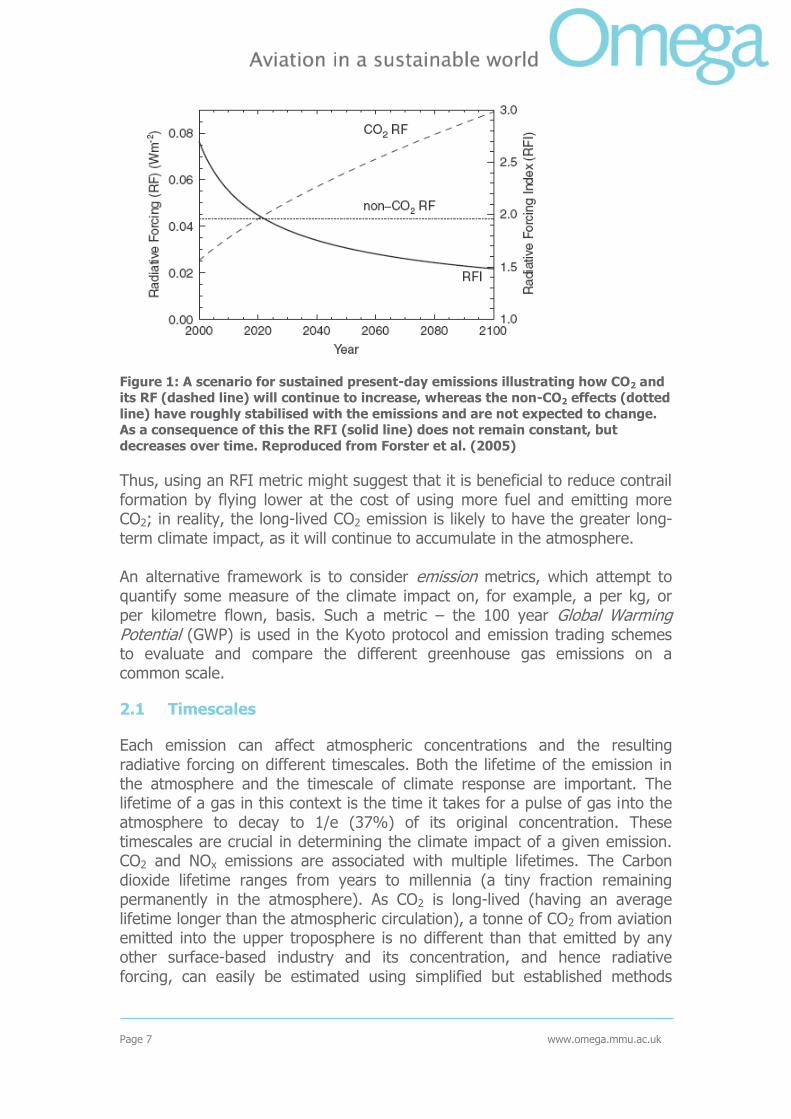
Radiative forcing evaluates the perturbation to the Earth‟s radiation balance since pre-industrial times. The forcing is due to the remaining concentrations of all radiatively-active species in the atmosphere as a result of all past emissions. As each of the exhaust gases have different atmospheric lifetimes, different amounts of emission contribute separately to each forcing. In the case of aviation, emissions of CO2 over many decades contribute to the CO2 radiative forcing. By contrast, for short-lived species such as ozone produced from NOx, it is the emissions in the few weeks prior to the target date of interest that contribute. Therefore the values of radiative forcing from two different gases cannot be easily related to emissions. CO2 has a complex atmospheric lifetime, varying from decades to millennium, whilst NOx, ozone and methane are much shorter lived gases with lifetimes of a few hours, weeks and 10 years respectively. The effects of NOx in the atmosphere depend on the season and latitude in which it is emitted. The IPCC6 introduced a metric, the „radiative forcing index‟, RFI, as one way of characterising the importance of non-CO2 forcings from aviation. It is simply the ratio of the total forcing to the CO2-only forcing. Regrettably, the concept has been miss-applied as a measure of the relative impact of non-CO2 species of emissions at a given time7 8. Present day radiative forcing is affected by emissions from many different time periods in the past; this is why measures such as the RFI should not be used to assess present emissions. An illustration of this is for a hypothetical case which assumes current emissions are sustained at a constant level. The radiative forcing from CO2 will continue to increase, whereas the other forcings remain more-or-less constant. Thus RFI decreases over time (see Figure 1) and the current RFI substantially overestimates the role of non-CO2 effects at, say, the 100 year time horizon used in the Kyoto protocol.

4 Stevenson DS, et al., Radiative forcing from aircraft NOx emissions: mechanisms and seasonal dependence. Journal of Geophysical Research 2004, 109:D17307 5 Wild O, et al., Indirect long-term global radiative cooling from NOx emissions. Geophysical Research Letters 2001, 28:1719-1722 6 IPCC. Aviation and the Global Atmosphere, A Special Report of IPCC (Intergovernmental Panel on Climate Change), Cambridge University Press, Cambridge, UK. 1999. 7 Forster PMdeF, et al., It is premature to include non-CO2 effects of aviation in emission trading schemes. Atmospheric Environment, 2006 8 Forster PMdeF, et al., Corrigendum to "It is premature to include non-CO2 effects of aviation in emission trading schemes". Atmospheric Environment, 2007

www.omega.mmu.ac.uk

Figure 1: A scenario for sustained present-day emissions illustrating how CO2 and its RF (dashed line) will continue to increase, whereas the non-CO2 effects (dotted

line) have roughly stabilised with the emissions and are not expected to change. As a consequence of this the RFI (solid line) does not remain constant, but

decreases over time. Reproduced from Forster et al. (2005)

Thus, using an RFI metric might suggest that it is beneficial to reduce contrail formation by flying lower at the cost of using more fuel and emitting more CO2; in reality, the long-lived CO2 emission is likely to have the greater long-term climate impact, as it will continue to accumulate in the atmosphere. An alternative framework is to consider emission metrics, which attempt to quantify some measure of the climate impact on, for example, a per kg, or per kilometre flown, basis. Such a metric – the 100 year Global Warming Potential (GWP) is used in the Kyoto protocol and emission trading schemes to evaluate and compare the different greenhouse gas emissions on a common scale.

2.1 Timescales

Each emission can affect atmospheric concentrations and the resulting radiative forcing on different timescales. Both the lifetime of the emission in the atmosphere and the timescale of climate response are important. The lifetime of a gas in this context is the time it takes for a pulse of gas into the atmosphere to decay to 1/e (37%) of its original concentration. These timescales are crucial in determining the climate impact of a given emission. CO2 and NOx emissions are associated with multiple lifetimes. The Carbon dioxide lifetime ranges from years to millennia (a tiny fraction remaining permanently in the atmosphere). As CO2 is long-lived (having an average lifetime longer than the atmospheric circulation), a tonne of CO2 from aviation emitted into the upper troposphere is no different than that emitted by any other surface-based industry and its concentration, and hence radiative forcing, can easily be estimated using simplified but established methods

www.omega.mmu.ac.uk

based on carbon-cycle modelling9. In contrast, timescales associated with aviation NOx emissions are different than those associated with NOx emissions at the surface. Stevenson et al10 presents a useful discussion of the various timescales. Initially NOx produces ozone on short timescales (weeks-months), but it also decreases CH4, which has an associated timescale of roughly 12 years. As methane in turn also affects ozone, there is also a component of ozone change that occurs on this longer timescale. Contrails, in contrast, only last for a few hours. The timescale of climate response is the time it takes for the Earth‟s surface (particularly the ocean) to respond, so only 37% of the equilibrium response remains. This response also has multiple timescales, but can be approximated as roughly 10 years.

2.2 Calculation of appropriate climate metrics for aviation

Before describing the range of impacts that aviation has on climate, we briefly outline the basis of the metric that is commonly used to give a first-order description of the climate impacts of changes in the abundance of gases and aerosols. This is the „radiative forcing of climate‟, or „radiative forcing‟ (RF). RF describes the perturbation to the energy balance of the climate system on, for example, increasing the concentration of carbon dioxide or the coverage of contrails; it is expressed in Wm-2. The basic usefulness of RF as a concept is its ability to compare forcings arising from very different phenomena (e.g. changes in greenhouse gas concentrations, particles, clouds, solar irradiance, land-use etc.). This is because the following property has been established from many climate modelling studies:

∆Ts λ RF. (1)

That is, there is an approximately linear relationship between the global mean radiative forcing (RF), λ, and the global mean equilibrium surface temperature change (∆Ts); λ is the climate sensitivity parameter (K (W m-2)-1), the “constant” of proportionality between forcing and temperature change. A positive RF implies warming; negative, cooling.

Aviation affects RF in the following ways:

positively (warming) by emissions of CO2; positively by tropospheric ozone (O3) (via atmospheric chemistry

from emissions of nitrogen oxides - NOx); negatively (cooling) by the reduction of ambient methane (CH4) (via

atmospheric chemistry from emissions of NOx); negatively by sulphate particles arising from sulphur in the fuel; positively by emissions of soot particles;

9 Op. cit. Shine, K.P., et al., 2005 10 Op. cit. Stevenson DS, et al.

www.omega.mmu.ac.uk

positively by linear persistent contrails (condensation trails) formed in the wake of the aircraft;

positively by enhanced cirrus cloud coverage formed from spreading contrails. Additional cloud condensation nuclei (particles) introduced into the upper troposphere by aircraft exhaust emissions could also influence natural cirrus clouds, probably causing a positive forcing, but little research has been done in this area.

It should be realised that RF is a quite different metric to the Global Warming Potential (GWP), the latter being a policy metric that allows a comparison to be made between the marginal impact of the addition of an emission of a gas relative to that of CO2

11. However, the RF concept underlies GWPs, since GWPs use the radiative efficiency (W m-2 kg-1) of an increase in abundance of a gas, cloud or aerosol. Climate metrics and their science and policy applications have been discussed in great detail by Fuglestvedt et al.12 and in an aviation context by Wit et al. 13.

2.2.1 The Pulse Global Warming Potential

The standard climate metric proposed by the Intergovernmental Panel on Climate Change14, and adopted by the Kyoto Protocol, is the Global Warming Potential (GWP); this is time integrated radiative forcing due to a pulse emission of a unit mass of gas. The use of the GWP is now deeply embedded and in widespread acceptance by the user community for the Kyoto group of greenhouse gases. For clarity, this will henceforth be referred to as the pulse GWP (PGWP). It can be quoted as an absolute PGWP (APGWP) (e.g. in units of Wm-2kg-1year) or as a dimensionless value by dividing the APGWP by the APGWP of a reference gas, normally CO2. A user choice is the “time horizon” over which the integration is performed. There is no obvious choice for this; the Kyoto Protocol chooses a 100 year GWP. For a gas x, if Ax is the radiative

forcing per kg, x is the lifetime of the gas, and H is the time horizon then:

H

xxx

xx

x HAdttAHAPGWP0

)]exp(1[)exp()(

(2)

The APGWP for CO2 is more complicated, because its atmospheric lifetime cannot be represented by a simple exponential decay. The APGWP for CO2 is not given here, but it can be found, for example, in Appendix A of Shine et al.(2005); the APGWP used by IPCC15 is adopted.

11 IPCC. Climate Change. The IPCC Scientific Assessment, Intergovernmental Panel on Climate Change, Cambridge University Press, UK. 1990. 12 Op. cit. Fuglestvedt, J.S., et al. 2003 13 Wit RCN, et al., Giving wings to emission trading. Inclusion of aviation under the European emission trading system (ETS): design and impacts. CE-Delft, No. ENC.C.2/ETU/2004/0074r, the Netherlands. 2005. 14 IPCC, Climate Change 2001, The Scientific Basis. Intergovernmental Panel on Climate Change, Cambridge University Press, UK, 2001. 15 Ibid.

www.omega.mmu.ac.uk

As stated, Ax is the radiative forcing per kg of emitted gas and x is the

emitted gases lifetime. In the case of NOx, where the radiatively active species are not directly emitted, the lifetime used is that of NOx (0.1 years) for short-lived ozone effects and that of methane (11.53 years) for longer lived effects. In this case, Ax values for ozone and methane are then inferred from time-integrated radiative forcings evaluated using chemical transport models. For contrails and cloud effects, there is no appreciable lifetime or emission source. In these cases the emission of CO2 in one year is assumed to cause all the calculated radiative forcing, but only within the same year.

2.2.2 The Global Temperature Change Potentials

A more recently proposed group of metrics16are the pulse and sustained Global Temperature Change Potential (PGTP and SGTP) which have rather different characteristics (they are “end-point” metrics – i.e. the temperature change at a particular time in the future, rather than a time integrated one). Arguably the GTPs are more relevant, as they address an actual climate impact (temperature change), rather than the more abstract integrated radiative forcing. A disadvantage is that they are not accepted for widespread use. To allow a transparent formulation of the GTPs, Shine et al. (2005) adopted a simple climate model which allowed analytical forms of the GTPs to be derived, although this is by no means a requirement. The inclusion of this climate model means that additional parameters are required to be defined – the timescale of the climate response, τ, and the heat capacity of the climate system, C (or equivalently, C and the climate sensitivity parameter, λ – the three parameters are related since τ=Cλ). The APGTP for gas x is given by:

)]exp()[exp()(

)(11

HHC

AHAPGTP

xx

xx

(3)

Again, a more complex relationship is required for CO2 and (2.4) is only

applicable provided τ is not equal to . Details are given in Shine et al. (2005) Shine et al. (2005) point out that although the pulse form of the GTP has some appeal, it appears that the simple climate model does not well represent the response of the climate system to a pulse emission; it will be

retained here for illustrative purposes only. Also, for any case where H >> x (which is often the case for aviation emissions), the PGTP will be very small, as the climate system will have “forgotten” about the pulse emission. However, Shine et al.17 have proposed an alternative use of the PGTP, consistent with EU policy of restricting warming below some target amount at

16 Op. cit. Shine, K.P., et al., 2005 17 Shine KP, et al., Comparing the climate effect of emissions of short- and long-lived climate agents. Accepted for publication in Phil. Trans. R.Soc. 2007.

www.omega.mmu.ac.uk

some future time. This application shows clearly that as the target is approached, it becomes more “valuable” to reduce short-lived emissions. At times well before the target time, it is the long-lived species that exert more influence on the temperature at the target time. Instead of a pulse emission being applied to the GTP, the ASGTP uses „sustained‟ emissions, applied constantly over the whole time horizon being investigated. Whilst a pulse emission will affect temperature for a short while before returning to the equilibrium state, a sustained emission will cause a permanent temperature perturbation. The ASGTP for gas x is given by

)]exp()[exp()(

1)]exp(1[)(

11

HHHC

AHASGTP

xx

xxx (4)

Shine et al. (2005) provide details of the CO2 and τ= cases. As detailed by

Shine et al. (2005) and, for long time horizons, the PGWP and SGTP asymptote to the same result. This allows an alternative interpretation of the GWP, and makes the distinction between the choice of pulse and sustained emissions arguably less important.

2.2.3 Discussion of Uncertainties

Even though aviation GWPs are readily calculable, there is considerable controversy about the application of emission metrics to assess the effect of aviation non-CO2 emissions. IPCC18 stated that the GWP “has flaws that make its use questionable for aviation emissions” and that “there is a basic impossibility of defining a GWP for aircraft NOx”. Wit et al.19 echo these sentiments, concluding that “GWPs are not a useful tool for calculating the complete suite of aircraft effects”. An undesirable side effect of the negative stance is that it has led some policymakers and other groups to apply the RFI as if it is some kind of alternative to the GWP20. Others have taken a more pragmatic stance than IPCC, and attempted to develop GWPs for aviation emissions, whilst recognising the caveats. The first attempt appears to be by H.Klug and colleagues in a series of unpublished reports as part of the EC Framework 5 Cryoplane project. More recently Svennson et al.21 have provided GWP values for aviation, based partly on the Klug approach. Wild et al.22 and Stevenson et al.23 have generated GWP values (although they did not label them as such) for aviation NOx emissions.

18 Op. cit. IPCC ,1999 19 Op. cit. Wit et al. 20 Op. cit. Forster PMdeF, et al., 2006 21 Svensson F, et al., Reduced environmental impact by lowered cruise altitude for liquid hydrogen-fuelled aircraft. Aerospace Science and Technology, 2004, 8:307-320 22 Op. cit. Wild et al. 23 Op. cit. Stevenson et al

www.omega.mmu.ac.uk

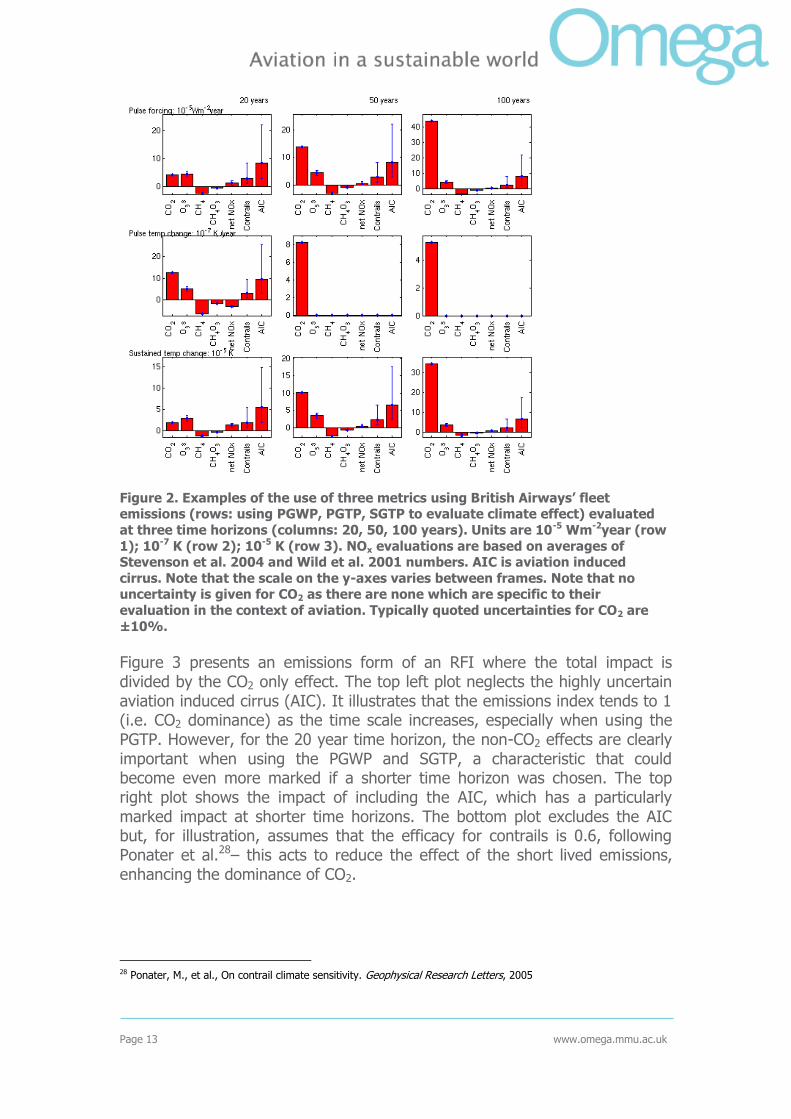
Forster et al.24 25 have also generated GWP values for a range of aviation emissions. They are also quoted in the latest IPCC report26. Uncertainties also need to be assessed when evaluating metrics. In particular more uncertain effects should not necessarily be given an equal weight to the role of carbon dioxide emissions in which we have a good level of confidence. These uncertainties are indicated by error-bars for NOx and contrails. Using fleet emissions data from British Airways27, figure 2 shows that at the 20-year time horizon, the short lived emissions are competitive with CO2 for all three metrics. The net NOx effect varies between the cases but all three metrics tell a generally similar story. At longer time horizons, CO2 becomes increasingly dominant, especially using the PGTP. The values using PGWP and SGTP become increasingly similar at long time horizons.

24 Op. cit. Forster PMdeF, et al., 2006 25 Op. cit. Forster PMdeF, et al., Atmospheric Environment, 2007 26 Forster P, et al., Changes in Atmospheric Constituents and in Radiative Forcing. In: Climate Change 2007: The Physical Science Basis. 27 Forster, P, and Rogers, H. Metrics for comparison of climate impacts from well mixed greenhouse gases and inhomogeneous forcing such as those from UTRLS ozone, contrails and contrail cirrus. 2008.

www.omega.mmu.ac.uk

Figure 2. Examples of the use of three metrics using British Airways’ fleet emissions (rows: using PGWP, PGTP, SGTP to evaluate climate effect) evaluated

at three time horizons (columns: 20, 50, 100 years). Units are 10-5 Wm-2year (row

1); 10-7 K (row 2); 10-5 K (row 3). NOx evaluations are based on averages of Stevenson et al. 2004 and Wild et al. 2001 numbers. AIC is aviation induced

cirrus. Note that the scale on the y-axes varies between frames. Note that no uncertainty is given for CO2 as there are none which are specific to their

evaluation in the context of aviation. Typically quoted uncertainties for CO2 are

±10%.

Figure 3 presents an emissions form of an RFI where the total impact is divided by the CO2 only effect. The top left plot neglects the highly uncertain aviation induced cirrus (AIC). It illustrates that the emissions index tends to 1 (i.e. CO2 dominance) as the time scale increases, especially when using the PGTP. However, for the 20 year time horizon, the non-CO2 effects are clearly important when using the PGWP and SGTP, a characteristic that could become even more marked if a shorter time horizon was chosen. The top right plot shows the impact of including the AIC, which has a particularly marked impact at shorter time horizons. The bottom plot excludes the AIC but, for illustration, assumes that the efficacy for contrails is 0.6, following Ponater et al.28– this acts to reduce the effect of the short lived emissions, enhancing the dominance of CO2.

28 Ponater, M., et al., On contrail climate sensitivity. Geophysical Research Letters, 2005

www.omega.mmu.ac.uk

Figure 3. Summary of figure 2, where total aviation impact has been normalized to CO2 impact creating an emission weighting factor appropriate to the current fleet.

Error bars present uncertainties arising from NOx and contrail forcings. Top:

excluding the highly uncertain aviation induced cirrus (AIC). Middle: Including AIC. Bottom: Excluding AIC, and assuming an efficacy of 0.6 for contrail forcing.

Note that the scale on the y-axes varies between frames.

The effects of contrails on cirrus clouds certainly do preclude confident evaluation of values of GWPs, but the problem is much deeper than the evaluation of metrics – any attempt to quantify their impact, using even the most sophisticated climate models, would face similar limitations (table 1). Table 1 represents the “per kg emitted” metrics. To evaluate the actual impact of a fleet these values must be multiplied by the actual mass emissions. Table 1. Absolute values of defined climate metrics for three different time horizons. Units: APGWP * 10-14 W m-2 kg(NO2)-1 yr. APGTP * 10-16 K kg (NO2)

-1.

ASGTP * 10-14 K (kg(NO2)-1)-1. Values for contrails, assuming 10 mWm-2 for 550 Tg

CO2, factor of three uncertainty. Values for aviation induced cirrus assuming 30

mWm-2 for 550 Tg CO2, range based on an RF between 10 mWm-2 and 80 mWm-2.

These ranges are taken from Forster et al.29, Table 2.9.

Contrails Aviation induced cirrus

20 yr 100 yr 500 yr 20 yr 100 yr 500 yr

APGWP APGTP ASGTP

1.8 1.8 1.8 5.5 5.5 5.5

2.1 0.0 0.0 6.3 0.0 0.0

1.2 1.5 1.5 3.7 4.4 4.4

29 Op. cit. Forster P, et al., 2007

www.omega.mmu.ac.uk

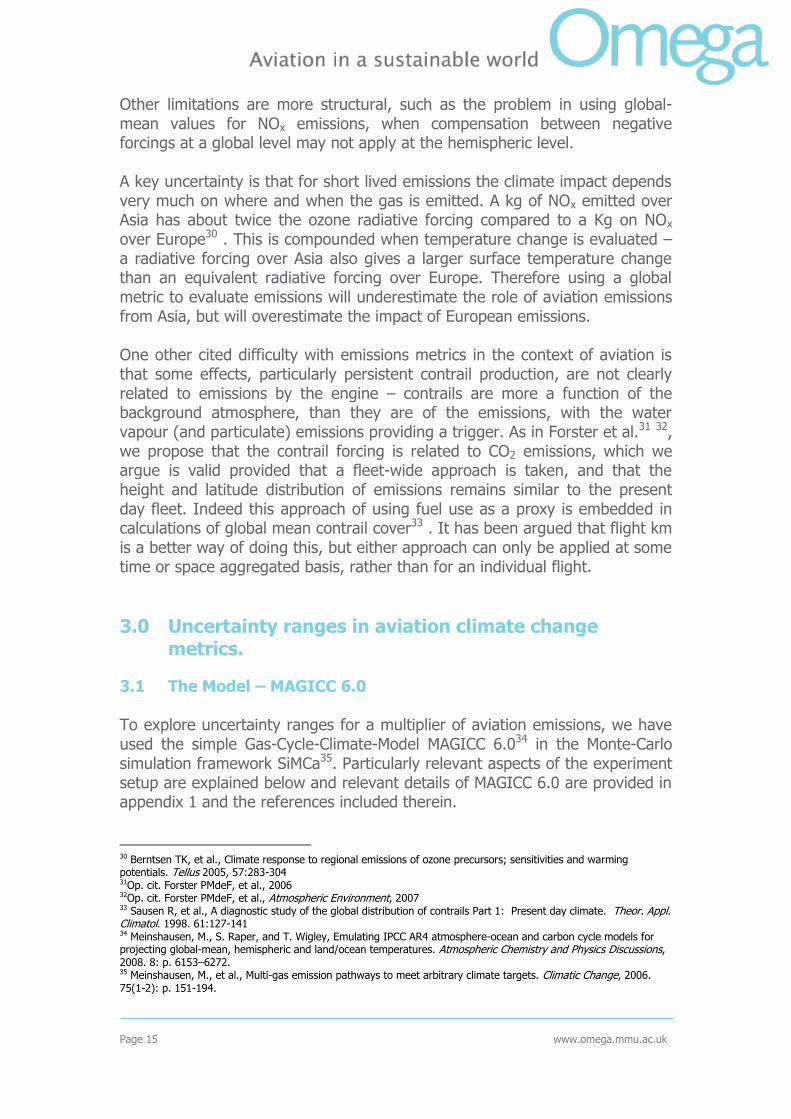
Other limitations are more structural, such as the problem in using global-mean values for NOx emissions, when compensation between negative forcings at a global level may not apply at the hemispheric level. A key uncertainty is that for short lived emissions the climate impact depends very much on where and when the gas is emitted. A kg of NOx emitted over Asia has about twice the ozone radiative forcing compared to a Kg on NOx over Europe30 . This is compounded when temperature change is evaluated – a radiative forcing over Asia also gives a larger surface temperature change than an equivalent radiative forcing over Europe. Therefore using a global metric to evaluate emissions will underestimate the role of aviation emissions from Asia, but will overestimate the impact of European emissions. One other cited difficulty with emissions metrics in the context of aviation is that some effects, particularly persistent contrail production, are not clearly related to emissions by the engine – contrails are more a function of the background atmosphere, than they are of the emissions, with the water vapour (and particulate) emissions providing a trigger. As in Forster et al.31 32, we propose that the contrail forcing is related to CO2 emissions, which we argue is valid provided that a fleet-wide approach is taken, and that the height and latitude distribution of emissions remains similar to the present day fleet. Indeed this approach of using fuel use as a proxy is embedded in calculations of global mean contrail cover33 . It has been argued that flight km is a better way of doing this, but either approach can only be applied at some time or space aggregated basis, rather than for an individual flight.

3.0 Uncertainty ranges in aviation climate change metrics.

3.1 The Model – MAGICC 6.0 To explore uncertainty ranges for a multiplier of aviation emissions, we have used the simple Gas-Cycle-Climate-Model MAGICC 6.034 in the Monte-Carlo simulation framework SiMCa35. Particularly relevant aspects of the experiment setup are explained below and relevant details of MAGICC 6.0 are provided in appendix 1 and the references included therein.

30 Berntsen TK, et al., Climate response to regional emissions of ozone precursors; sensitivities and warming potentials. Tellus 2005, 57:283-304 31Op. cit. Forster PMdeF, et al., 2006 32Op. cit. Forster PMdeF, et al., Atmospheric Environment, 2007 33 Sausen R, et al., A diagnostic study of the global distribution of contrails Part 1: Present day climate. Theor. Appl. Climatol. 1998. 61:127-141 34 Meinshausen, M., S. Raper, and T. Wigley, Emulating IPCC AR4 atmosphere-ocean and carbon cycle models for projecting global-mean, hemispheric and land/ocean temperatures. Atmospheric Chemistry and Physics Discussions, 2008. 8: p. 6153–6272. 35 Meinshausen, M., et al., Multi-gas emission pathways to meet arbitrary climate targets. Climatic Change, 2006. 75(1-2): p. 151-194.

www.omega.mmu.ac.uk

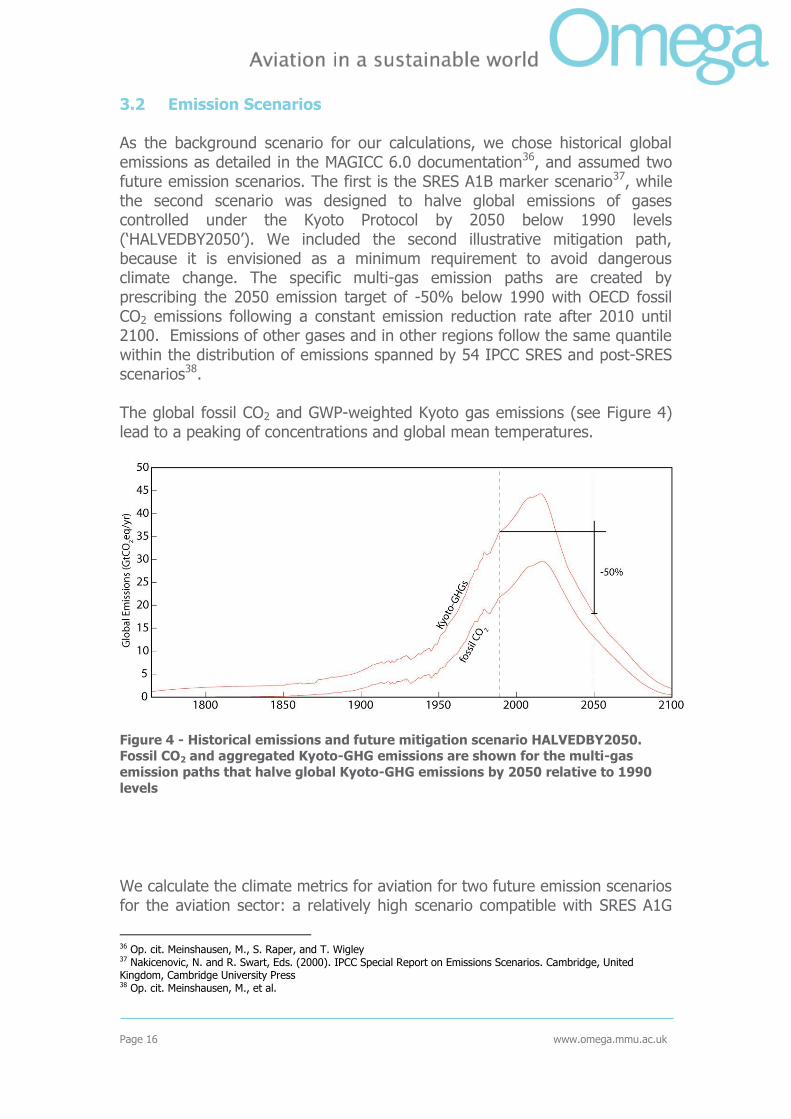
3.2 Emission Scenarios As the background scenario for our calculations, we chose historical global emissions as detailed in the MAGICC 6.0 documentation36, and assumed two future emission scenarios. The first is the SRES A1B marker scenario37, while the second scenario was designed to halve global emissions of gases controlled under the Kyoto Protocol by 2050 below 1990 levels („HALVEDBY2050‟). We included the second illustrative mitigation path, because it is envisioned as a minimum requirement to avoid dangerous climate change. The specific multi-gas emission paths are created by prescribing the 2050 emission target of -50% below 1990 with OECD fossil CO2 emissions following a constant emission reduction rate after 2010 until 2100. Emissions of other gases and in other regions follow the same quantile within the distribution of emissions spanned by 54 IPCC SRES and post-SRES scenarios38. The global fossil CO2 and GWP-weighted Kyoto gas emissions (see Figure 4) lead to a peaking of concentrations and global mean temperatures.

Figure 4 - Historical emissions and future mitigation scenario HALVEDBY2050. Fossil CO2 and aggregated Kyoto-GHG emissions are shown for the multi-gas

emission paths that halve global Kyoto-GHG emissions by 2050 relative to 1990

levels

We calculate the climate metrics for aviation for two future emission scenarios for the aviation sector: a relatively high scenario compatible with SRES A1G

36 Op. cit. Meinshausen, M., S. Raper, and T. Wigley 37 Nakicenovic, N. and R. Swart, Eds. (2000). IPCC Special Report on Emissions Scenarios. Cambridge, United Kingdom, Cambridge University Press 38 Op. cit. Meinshausen, M., et al.

www.omega.mmu.ac.uk

as assessed by MESSAGE39 and a relatively low scenario in accordance with SRES A2-A1 as evaluated by MINICAM40. By default we will evaluate the SRES A1B background combined with the A2-A1 aviation scenario. We will examine the sensitivity of our results by evaluating further A1B combined with A1G and HALVEDBY2050 combined with A2-A1. Combining HALVEDBY2050 with A1G was not implemented, because this implies that aviation emissions exceed global emissions by the end of the 21st century. All scenarios are extended to 2150 by fixing year-2100 emissions, in order to calculate the metrics with appropriate time horizon (next section).

3.3 Calculation of GWP and GTP metrics For each of the 1500 parameter sets drawn at random, the full anthropogenic global total emission pathway is run, where emissions from the aviation sector are subtracted from the global emissions baseline („BASE‟ simulation). Subsequently, the simulation is repeated with the same sequence of randomly drawn parameter values, but aviation emissions in year T are not subtracted (all-emissions pulse: „ALL‟). The paired differences between these two simulations then provide the distribution of the likely residual contribution of an aviation emission pulse in year T to radiative forcing and global-mean temperature change. Finally, the simulation is repeated for an emission pulse of only CO2 in year T („CO2‟). Comparison of the last simulation with the all-emission-pulse simulation allows calculating a multiplier for the climate effects of all aviation emissions relative to CO2-only, for each paired run n in the simulations:

(5)

In which T is the year of the emission pulse, is the radiative forcing in

year t in run n of experiment X (resp. the BASE, ALL-pulse, or CO2-pulse simulations). The multiplier for pulse GTP (2) is defined by:

(6)

The GTP is evaluated at a time Hn, defined as the year in which global-mean temperature increase reaches 2°C above pre-industrial in a baseline scenario without the aviation sector emissions subtracted. Like the other calculations,

39 Op. cit. Nakicenovic, N. and R. Swart, Eds. 40 Ibid.

www.omega.mmu.ac.uk

the GTP time horizon depends on the parameter values drawn in the Monte-Carlo simulations and is paired to the runs in the other simulations (hence subscript n). Note that the later the emission pulse, the more likely it will be that the 2°C temperature target is exceeded in the baseline scenario before the emission pulse year. In this case GTP is evaluated 1 year after the pulse, thereby giving maximum weight to short-lived species. In case the temperature target is nor exceeded by the end of the simulation in the year 2150, Hn is set at 2150. We will calculate statistics like medians and standard deviation over all runs to arrive at single indicator values for each emission-pulse year from 2010 to 2050 with 5 year steps. 3.4 Results 3.4.1 Global Warming Potentials

We classified the calculated Multiplier for GWP in 2010 in 30 bins, normalized to a total of 1. This produces an estimate of the posterior distribution for GWP multiplier as pictured in figure 5 for the A1B baseline, combined with A2-A1 MiniCam aviations emissions scenario. The distribution has standard deviation 0.5 and is somewhat skewed with a mean of 2.2 and a median of 2.1. A value close to 2 implies that the climate effects of non-CO2 emissions measured by GWP are about equal to the direct CO2 effects. Sensitivity experiments show that 5 to 15% of the response to non-CO2 emissions is caused by changes in CO2 radiative forcing, caused by C-Cycle changes induced by the temperature effects of non-CO2 emissions. A Multiplier of 2.1 SD 0.5 is consistent with the value of 1.7 found by Forster et al.41 42. Unlike our study, Forster et al.43 44 have evaluated a GWP Multiplier for other GWP time horizons and noted high sensitivity, because of the different weighting of short-lived climate effects of non-CO2 emissions relative to CO2. We will come back to that subject further on when discussing the results for GTP Multiplier.

41 Op. cit .Forster PMdeF, et al., 2006 42 Op. cit. Forster PMdeF, et al, Atmospheric Environment, 2007 43 Op. cit. Forster PMdeF, et al., 2006 44 Op. cit. Forster PMdeF, et al, Atmospheric Environment, 2007

www.omega.mmu.ac.uk

Figure 5 - Posterior distribution for 100-yr GWP Multiplier for baseline A1B and

aviation scenario A2-A1.

For the same baseline, figure 6 shows the estimated distribution for a 2010 emission pulse selected from the A2-A1 aviation scenario. With a mean of 2.1, a median of 2.0 and equal standard deviation, this aviation emission scenario produces a slightly lower relative impact of non-CO2 emissions. Thus, the dependence of GWP Multiplier estimate on the size of the emission pulse is small. The lower Multiplier value for higher aviation emission pulses is caused by increased saturation of contrail radiative forcing in the A1G aviation scenario, as is confirmed by a sensitivity test in which we have switched off contrail saturation. In this experiment the difference in Multiplier for the two aviation scenarios vanishes.

100-yr GWP Multiplier

www.omega.mmu.ac.uk

Figure 6 - Posterior distribution for 100-yr GWP Multiplier for baseline A1B and

aviation scenario A1G. For comparison the estimate in figure 5 for the A2-A1 aviation scenario is reproduced in open bars.

A similarly small sensitivity is apparent to the baseline scenario. In figure 7 we show the estimated distribution of the HALVEDBY2050 baseline and A2-A1 aviation scenario. With again equal standard deviation, a mean of 2.0 and median of 1.9, we conclude that the 100-yr GWP Multiplier is marginally sensitive to baseline scenario. The decrease of the Multiplier as the baseline concentration decreases is possibly caused by the lower saturation of CO2 radiative forcing. A lower saturation at lower background concentration means larger effects for equal emission-pulse size. For large CO2 effects the

Multiplier will approach the value 1 – when in equation (5) becomes

dominated by the CO2 part of it, the denominator and numerator of the GWP Multiplier converge.


www.omega.mmu.ac.uk

Figure 7 - Posterior distribution for 100-yr GWP Multiplier for baseline

HALVEDBY2050 and aviation scenario A2-A1. For comparison, the estimate in figure 5 for the A1B baseline scenario is reproduced in open bars

The results above were all produced by emissions pulses in the year 2010. Figure 8 shows that the 100-yr GWP Multiplier hardly depends on the year in which the emission pulse is released, and rises to from median 2.1 in 2010 to 2.2 by the year 2050. The uncertainty and skewness increase somewhat more, with mean rising from 2.2 to 2.4 and standard deviation from 0.5 to 0.7 over the 2010 to 2050 range.


www.omega.mmu.ac.uk

Figure 8 - Median and uncertainty ranges for 100-yr GWP Multiplier for emission

pulses between 2010 and 2050 with 5 year intervals. The baseline is A1B and the aviation scenario A2-A1.

3.4.2 Global Temperature Change Potentials For the A1B baseline combined with the A2-A1 MiniCam aviation scenario the Multiplier for 2°C-target GTP reaches a median of 1.2 for an emission pulse in the year 2010, with a standard deviation of 0.1 (Figure 9). Thus, the gradual decay of temperature response in the years following the emission pulse is fast enough to let GTP Multiplier be much lower than GWP Multiplier. For emission pulse year 2010, the GTP Multiplier exhibits comparable sensitivity to baseline and aviation emission scenario as the GWP Multiplier, including the sensitivity to saturation of contrail and CO2 radiative forcing. Therefore, we will focus here on the more interesting time behaviour of the GTP indicator.

www.omega.mmu.ac.uk

Figure 9 - Posterior distribution for 2°C target GTP Multiplier for baseline A1B and

aviation scenario A2-A1.

Until emission-pulse year 2030, the GTP Multiplier median is virtually constant (figure 10). The uncertainty on the high side starts to increase by the end of this period, once the first runs in the sample of 1500 begin to exceed the temperature target of 2°C. The median of the year in which the 2°C target is exceeded is 2049 in this scenario, with a standard deviation of 14 years. Thus, for an emission pulse in 2050, the global-mean temperature in roughly 50% of the runs has already surpassed the target before the emission pulse year is reached. Since short-lived gases will have their maximum effect when evaluated shortly after being emitted, the uncertainty on the high side starts to grow rapidly by the time the target is exceeded in some runs, in this case around 2035 (figure 11). This equals the target-year‟s estimated median of 2049 minus its standard deviation of 14 years. The median commences to rise rapidly somewhat later and reaches a value of around 20 for emission-pulse year 2050. By that time the rise in uncertainty on the high side starts to level off, as uncertainty ranges and median eventually should converge to constant values once the global temperature in all runs will have exceeded the 2°C target.

100-yr GTP Multiplier

www.omega.mmu.ac.uk

Figure 10 - Median and uncertainty ranges for 2°C Target GTP Multiplier for

emission pulses between 2010 and 2030 with 5 year intervals. The baseline is A1B and the aviation scenario A2-A1.

Figure 11 - Median and uncertainty ranges for 2°C Target GTP Multiplier for

emission pulses between 2010 and 2050 with 5 year intervals. The baselines are

A1B (orange & red) and HALVEDBY2050 (green), the aviation scenarios are A2-A1

www.omega.mmu.ac.uk

(orange and green) and A1G (red). Only the uncertainty ranges for A1B / A2-A1

are pictured.

As for GWP Multiplier and GTP Multiplier for emission-pulse year 2010, the sensitivity to aviation scenario at the end of our evaluation time range is small and mainly caused by saturation of contrail radiative forcing. This is confirmed by the same sensitivity experiments performed to test the sensitivity of the GWP Multiplier to aviation scenario. By contrast, the impact of later emission pulses depends very sensitively on baseline scenario, confirming the results of Shine et al.45. The reason behind this sensitivity is not a physical mechanism, but the result of a shifting evaluation year, since the 2°C temperature target is exceeded in a different year for a different baseline. For the HALVEDBY2050 baseline scenario the median of the temperature-target year is 2125, with standard deviation of 45 years. With the target year dated much later than the emission pulses, the GTP Multiplier‟s median hardly increases for later emission pulses. Even in this case, however, the uncertainty starts to increase in our experiments: the 90% uncertainty boundary on the high side reaches 33 in 2050 and the 70% high boundary reaches 17, indicating that even under this baseline the target is exceeded in a significant number of runs. 3.5 Conclusions to uncertainty ranges study The results presented in this section confirm earlier studies in terms of the „best-guess‟ value of a non-CO2 GWP multiplier46 47 of around 2 for the aviation sector. In addition, our results confirm earlier findings that the pulse GTP is smaller than GWP for short-lived species for emission years long before the evaluation (temperature target) year, whereas the GTP multiplier for short-lived species increases sharply as the time is approached at which the temperature target is exceeded48.

Adding to these findings is our estimate of the uncertainty range of the multipliers, including uncertainty in carbon-cycle and (simple) climate modeling parameters, as well as the effects of NOx emissions on methane and Ozone chemistry and climate. With this additional data, we estimate the multiplier for 100-yr GWP at about 2.0 with standard deviation 0.5. The 2°C target GTP multiplier is estimated at about 1.2 (SD 0.1) for emissions long before the evaluation year, while both the median value and uncertainty range increase sharply to 20 (SD 18) around the time of evaluation (temperature target year), these sharp increases starting about 15 years before the temperature target year. The dependency of the indicator values on both background and aviation emission scenario‟s is small, though the GTP

45 Op. cit. Shine KP, et al., 2007. 46 Op. cit. Forster PMdeF, et al., 2006 47 Op. cit. Forster PMdeF, et al, Atmospheric Environment, 2007 48 Op. cit. Shine KP, et al., 2007.

www.omega.mmu.ac.uk

multiplier is highly sensitive on the year in which the temperature target is reached and thus on background scenario.

4.0 The use of climate metrics to interpret NOx emissions from aviation

This section details a global modelling study to determine the non-CO2 atmospheric response due to perturbations in NOx. 4.1 The Model – p-TOMCAT The chemistry transport model pTOMCAT has been developed at the University of Cambridge (O‟Connor et al., 200549; Savage et al., 200450). The model reproduces realistically the transport and the chemistry of atmospheric tracers on global scale. The wind and temperature needed to calculate these processes are extracted from the ECMWF operational analyses (pTOMCAT is an off-line model). The model includes 48 species and 35 tracers. The advection of the 35 tracers is calculated using the highly conservative second order moment as described in Prather (1986)51. The convection parameterisation follows the Tiedtke (1989)52 scheme. The chemistry consists in 112 gas phase reactions, 27 photolysis rates and 1 heterogeneous reaction and represents the chemical processes relevant to the troposphere and the lower stratosphere. The model uses the chemistry integration package ASAD (Carver et al.,199753) and the ozone and nitrogen oxides are constrain at the top level of the model to values calculated by the Cambridge 2D model (Law and Nisbet, 199654). The pTOMCAT model has been used in international projects and has been subjected to validation and inter-comparison with other atmospheric models (Brunner et al., 2003; 200555,56). The version of the model used in OMEGA-METRIC is the same version used in the QUANTIFY project (Hoor et al., 200857). The resolution is T21-L31 (64 longitudes, 32 latitudes and 31 levels from the surface to 10hPa vertically). The anthropogenic and biogenic

49 O‟Connor, F., et al., Comparison and visualisation of high-resolution transport modelling with aircraft measurements, Atm. Sci. Lett., 6, 164-170, 2005. 50 Savage, N., et al, Using GOME NO2 satellite data to examine regional differences in TOMCAT model performance, Atmos. Chem. Phys., 4, 1895-1912, 2004. 51 Prather, M., Numerical advection by conservation of second-order moments, J. Geophys. Res., 91, 6671-6681, 1986. 52 Tiedtke, M, A comprehensive mass flux scheme for cumulus parameterisation on large scale models, Mon. Weather Rev., 117, 1779-1800, 1989. 53 Carver, G., P. Brown and O. Wild, The ASAD Atmospheric Chemistry Integration Package and Chemical Reaction Database, Comp. Physics Communications, 105, 197-215, 1997. 54 Law, K. and E. Nisbet, Sensitivity of the methane growth rate to changes in methane emissions from natural gas and coal, J. Geophys. Res., 101, 14387-14397, 1996. 55 Brunner, D., et al, An evaluation of the performance of chemitry transport models by comparison with research aircraft observations, 1, concept and overall model performance, Atmos. Chem. Phys., 3, 1609-1631, 2003. 56 Brunner, D., et al., An evaluation of the performance of chemitry transport models by comparison with research aircraft observations, 2, detailed comparison with two selected campaigns, Atmos. Chem. Phys., 5, 107-129, 2005. 57 Hoor, P.,et al, The impact of traffic emissions on atmospheric ozone and OH: results from QUANTIFY, Atmos. Chem. Phys. Discuss., 8, 18219-18266,2008.

www.omega.mmu.ac.uk

emissions have been produced within the QUANTIFY project and are representative of the year 2000 (table 2 for anthropogenic emissions) with focus on the anthropogenic emissions and in particular the transportation sector (Borken et al., 200758; Endresen et al., 200759; Lee et al., 200760). Figure 12 represents the geographical distribution of the respective anthropogenic emission of NOx: non-transport, road, shipping and aviation. Table2 : NOx anthropogenic emissions in Tg (1012g) for the year 2000 for

different sectors. Non transport = bio and fossil fuel combustion, fossil fuel production, industrial processes and waste. Shipping = maritime and inland shipping. Rail = direct and indirect emissions.

Year 2000 Road Shipping Aviation Non-transport NOx Tg/year 29.2 15.5 2.8 56.4

Figure 12: geographical distribution of NOx flux for the year 2000 in kg/month: A = aviation, B = international shipping, C = anthropogenic non-transport

emissions, D = road transport.

A set of 3 simulations has been done to study the impact of the NOx emissions from aviation: one base case (with all emissions except NOx emissions from aviation), one pulse case (the base case plus a pulse of NOx emissions from aviation for the month of January only) and finally one sustained case (with all emissions including NOx emissions from aviation). Each simulation begins with one year of spin-up (using 2001 meteorology) and 3 or 5 years of results (using 2002-2007 meteorology). The pulse of NOx occurs during January 2002 so the spin-up year is identical between the base

58 Borken, J., H. Steller, T. Meretei and F. Vanhove, Global and country inventory of road passenger and freight transportation – Their fuel consumption and their emissions of air pollutants in the year 2000, Transportation Research Records, Journal of the Transportation Research Board, 2011, 127-136, 2007. 59 Endresen, O., E. Sorgard, H. Behrens, P. Brett and I. Isaksen: A historical reconstruction of ships‟ fuel consumption and emissions, J. Geophys. Res., 112, 2007. 60 Lee, D., B. Owen, C. Fishter, L. Lim, and D. Dimitriu, Allocation of international aviation emissions from scheduled air traffic – present day and historical (report 2 of 3), Manchester Metropolitan University, CATE-2005-3[c]-2, Manchester, UK.

www.omega.mmu.ac.uk

case and the pulse case whilst in the case of the sustained emissions the emissions of NOx begin in 2001 and are present throughout the simulation. The quantity of NOx emitted during the January month for the pulse is 0.23 Tg(NO2), the amount of NOx emitted per year in the case of the sustained simulation is 2.8 Tg(NO2) and is constant for the duration of the experiment (ie: no inter-annual variation is included).

Results from the pulse experiment (Figure 13) show the increase in the burden of NOx at a maximum 0.13Tg (NO2) in the month of the pulse (January), rapidly decreasing to a third of that maximum in February. The impact on ozone is an increase in the burden of 1,500 Tg in January and peaking at a maximum of 2,500 Tg in February. The burden then decreases rapidly during the following months. The change in the ozone concentration in the troposphere induces a change in the oxidising capacity of the atmosphere that impact on peroxyl radicals and methane. The increase in the ozone and HOx burden due to the NOx pulse triggers a reduction of the life-time of methane and consequently a reduction in its burden. The maximum reduction in methane is reached in September/October at ≈ 0.6 Tg(CH4). This perturbation has a very slow decay due to the longer life-time of methane in the atmosphere (on the order of 10 years in the pTOMCAT model). Figure 14 presents the zonal mean of the perturbation due to the NOx January pulse for the 3 first months of the simulation (not including spin-up). The changes in NOx concentration occurs at flight level over the Northern Hemisphere in January (maximum of 0.05 ppbv). The perturbation in the UTLS has almost disappeared by March. During the second month we can observe a reduction in the NOx concentration in the lower part of the troposphere of around 0.05 pptv. This reduction is due to the increase in ozone observed in January (0.6 ppbv) and February (1.0 ppbv), the oxidising capacity of the lower troposphere is modified by the transport of the ozone produced at higher altitudes. The transport of ozone can also seen towards the Southern Hemisphere mid-latitudes in March. The impact on the OH field has a life-time of approximately a month.

www.omega.mmu.ac.uk

Figure 13: time evolution of the perturbation in the global burden of NOx, O3, CH4

and HOx due to a pulse of aircraft NOx emissions in January.

Figure 14: zonal-monthly mean distributions of NOx, O3 and OH perturbation due to a pulse of aircraft NOx emissions in January (from left: January, February and

March).

The results of the sustained emissions are presented in figure 15 as change in the global burden and figure 16 as a change in the monthly mean concentration of NOx, O3 and OH. The results are plotted over time from January 2001 to December 2007, the first year is used as spin-up for the model. The burden change of NOx varies seasonally from 0.4Tg(NOx) at its

www.omega.mmu.ac.uk

maximum in summer to a minimum of 0.2Tg in winter. This seasonality is not due to changes in emissions from aviation, there is less than a 3% variation in the difference between the maximum and minimum monthly mean emission from aviation, but is due to changes in the life-time of NOx in the UTLS between summer and winter (i.e.chemistry). The ozone impact follows the seasonality with approximately one month delay as seen in the pulse simulation (figure 13, where the pulse in January is followed by a maximum ozone change in February) the maximum is 10,000Tg(O3) and is dependent on the yearly meteorological conditions. The burden change in methane, which has not reach steady state after 7 years of simulation, is driven by the ozone change. The global burden decrease would be in the order of 35,000Tg (CH4) due to current NOx emissions from aviation.

Figure 15: time evolution of the perturbation in the global burden of NOx, O3, CH4 and HOx due to sustained aircraft NOx emissions.

www.omega.mmu.ac.uk

Figure 16: zonal-monthly mean distribution of NOx, , O3 and OH perturbation due to sustained aircraft NOx emission (from left: January, February and March).

The atmospheric response to the emitted NO2 is to undergo a process of oxidation to form O3. As described in section 2.2, the O3 can affect the radiative forcing capacity of the atmosphere in a number of direct and indirect ways. Directly, the O3 can be transported away from the region of emission and encourages global warming. Indirectly, negative forcing can take place as CH4 is formed from the further oxidation and breakdown of O3 via OH.

The calculated O3 fields from the p-TOMCAT experiments are used to calculate the instantaneous radiative forcing. The Edward-Slingo radiation code was employed here, and has been used in many other studies61 62 .This yields an upward or longwave forcing which is adjusted to take account of the stratospheric influence on temperature, and a downward or short-wave forcing. The sum of these two forcings provides the net climate forcing due to aviation effects.

4.2 Results 4.2.1 The pulse experiment

Figure 17 shows the radiative forcing owing to the 0.23 Tg pulse emission of aviation NOx at the tropopause. Whilst all the units are in W m-2, note that the legend for each of the maps is different, simply because of the factor of 4

61 Op. cit. Stevenson DS, et al. 62 Op. cit. Wild O, et al.

www.omega.mmu.ac.uk

difference between the first and subsequent months. This highlights how quickly the pulse in aviation emissions is oxidised by the atmosphere.

Jan W m-2 Feb W m-2

Mar W m-2

May W m-2 Jun W m-2

Apr W m-2

0

0.03

0.025

0.02

0.015

0.01

0.005

0.035

0.04

0

0.03

0.025

0.02

0.015

0.01

0.005

0.035

0.04

-5E-4

0.0025

0.002

0.0015

0.001

0.0005

0

0.003

0.0035

0.013

0.012

0.011

0.01

0.009

0.008

0.007

0.006

0.005

0.004

0.003

0.002

0.001

0

0.006

0.0055

0.005

0.045

0.004

0.0035

0.003

0.0025

0.002

0.0015

0.001

0.0005

0

-5E-4

0.0045

0.004

0.0035

0.003

0.0025

0.002

0.0015

0.001

0.0005

0

-5E-4

Jan W m-2 Feb W m-2

Mar W m-2

May W m-2 Jun W m-2

Apr W m-2

Jan W m-2 Feb W m-2

Mar W m-2

May W m-2 Jun W m-2

Apr W m-2

0

0.03

0.025

0.02

0.015

0.01

0.005

0.035

0.04

0

0.03

0.025

0.02

0.015

0.01

0.005

0.035

0.04

0

0.03

0.025

0.02

0.015

0.01

0.005

0.035

0.04

0

0.03

0.025

0.02

0.015

0.01

0.005

0.035

0.04

-5E-4

0.0025

0.002

0.0015

0.001

0.0005

0

0.003

0.0035

-5E-4

0.0025

0.002

0.0015

0.001

0.0005

0

0.003

0.0035

0.013

0.012

0.011

0.01

0.009

0.008

0.007

0.006

0.005

0.004

0.003

0.002

0.001

0

0.013

0.012

0.011

0.01

0.009

0.008

0.007

0.006

0.005

0.004

0.003

0.002

0.001

0

0.006

0.0055

0.005

0.045

0.004

0.0035

0.003

0.0025

0.002

0.0015

0.001

0.0005

0

-5E-4

0.006

0.0055

0.005

0.045

0.004

0.0035

0.003

0.0025

0.002

0.0015

0.001

0.0005

0

-5E-4

0.0045

0.004

0.0035

0.003

0.0025

0.002

0.0015

0.001

0.0005

0

-5E-4

0.0045

0.004

0.0035

0.003

0.0025

0.002

0.0015

0.001

0.0005

0

-5E-4

Figure 17. Maps to show the monthly position of radiative forcing at the

tropopause due to the pulse aviation emission over the north Atlantic corridor. All units in W m-2.

In January, the peak in net radiative forcing is located within the flight corridor between the Americas and Europe. By February this peak value is at the pulse experiment maximum of 40 mW m-2, though up to 35 mW m-2 is experienced in a longitudinal band circling 15-30°N. In March this peak value has decreased to 13 mW m-2, and the effects of the January pulse aviation emission are starting to spread laterally towards the equator and poles. By April the peak radiative forcing is reduced to 6 mW m-2. By May and June transport of the O3 towards the poles has located the peak radiative forcing

www.omega.mmu.ac.uk

effects here. Peaks of 4 mW m-2 occur north of the US and Canada, and the forcing in the north Atlantic flight corridor is now less than 1.5 mW m-2.

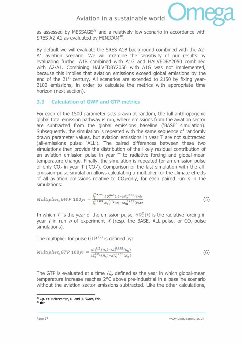
The radiative forcing maps in figure 17 are useful in pinpointing the location of the hotspots, but do not show what the effects on the world as whole are. Plotting the average radiative forcing values at the tropopause in figure 18 as a time series shows the difference between the net radiative forcing in the northern and southern hemispheres. The transition between short term positive forcing and the longer term „tail‟ of negative forcing is also highlighted here. In the northern hemisphere, the point of the transition occurs 12 months after the emission pulse was released. Although not visible on the same scale as the short term peak, the long term trough reaches -0.03 mW m-2, 32 months after the pulse aviation emission.

-2

0

2

4

6

8

10

12

14

16

Jan-02 Jan-03 Jan-04 Jan-05

Date

Ra

dia

tiv

e F

orc

ing

, m

W m

-2

net NH

net SH

net Global

Figure 18. Time series to show transition between positive and negative radiative

forcing for the northern and southern hemispheres, after the pulse in aviation emissions. Note that values used here are hemisphere averages.

Two previous studies by Stevenson et al.63and Wild et al.64 alculated values for aviation metrics. Similar aviation pulse emissions were released into the respective models (HADAM3 with STOCHEM in the case of Stevenson et al., and the University of California at Irvine CTM in the case of Wild et al.) and the impacts were integrated out to 100 years. The global warming potential was calculated for each of the process effects: short term O3 production due to NOx, long term O3 loss due to the loss of CH4, and the effects due to CH4

63 Op. cit. Stevenson DS, et al. 64 Op. cit. Wild O, et al.

www.omega.mmu.ac.uk

loss directly. The values are normalised to a 1 Tg emission of NOx, and compared to those of the Stevenson et al. and Wild et al. studies (table 3). Table 3. Comparison of radiative forcing metrics calculated by this study,

Stevenson et al. 65 and Wild et al. 66 The values include stratospheric adjustment, and have been normalised to a 1 Tg NO2 pulse emission. Based on table 4 within

Stevenson et al.

OMEGA

Stevenson et al.

Wild et al.

ΔCH4 lifetime, years 11.11 11.53 11.8

Total, ppbv yr -10.5 -11.3 -12.2

Radiative Forcing mW m-2 yr

-3.88 -4.2 -4.6

ΔO3 Short term Total, ppbv yr 0.39 0.23 0.36


4.26 5.06 7.9

ΔO3 Long term Total, ppbv yr -0.18 -0.044 -0.067


-1.45 -0.95 -1.5

Net Radiative Forcing mW m-2 yr

-1.07 -0.09 +1.8

The differences are due to the different model setup and dynamics used, as the input of aviation NOx was the same. In general, the values calculated by this Omega study are lower than those calculated by either of the other studies. The net global negative forcing of -0.09 mW m-2 yr predicted by Stevenson et al. sits between our Omega estimate of -1.07 mW m-2 yr and the warming of +1.8 mW m-2 yr predicted by Wild et al.. Thus, Omega predicts that an overall cooling will be expected from pulse emissions of NOx from aviation. The radiative forcing values in table 3 above can be applied to the climate change metrics APGWP, APGTP and ASGTP equations detailed in sections 2.2.1 and 2.2.2 earlier. We can also use the radiative forcing values calculated by Stevenson et al. and Wild et al. to provide a comparison after 20 years, 50 years and 100 years (Table 4).

65 Op. cit. Stevenson DS, et al. 66 Op. cit. Wild, et al.

www.omega.mmu.ac.uk

Table 4. Absolute values of defined climate metrics for three different time

horizons. Units: APGWP * 10-14 W m-2 kg(NO2)-1 yr. APGTP * 10-16 K kg (NO2)

-1. ASGTP * 10-14 K (kg(NO2)

-1)-1.

OMEGA Stevenson et al. Wild et al.

20 yr 50 yr 100 yr

20 yr 50 yr 100 yr

20 yr 50 yr 100 yr

NOx via CH4 loss

APGWP -324 -384 -388 -346 -415 -420 -376 -453 -460

APGTP -834 -133 -3 -899 -151 -3 -982 -171 -4

ASGTP -170 -293 -310 -180 -315 -336 -195 -344 -367

Short term O3 loss

APGWP 426 426 426 506 506 506 790 790 790

APGTP 496 30 0 589 36 0 920 56 1

ASGTP 288 338 341 342 401 405 534 626 632

Long term O3 loss

APGWP -121 -143 -145 -78 -94 -95 -122 -148 -150

APGTP -312 -50 -1 -203 -34 -1 -320 -56 -1

ASGTP -64 -109 -116 -41 -71 -76 -64 -112 -120

Sum of all NOx Effects

APGWP -19 -101 -107 82 -2 -9 292 189 180

APGTP -650 -153 -3 -514 -150 -4 -383 -171 -5

ASGTP 54 -65 -85 120 14 -7 275 169 145

The results from the Omega study are always lower than those from Stevenson et al. and Wild et al. Taking the sum of all effects into account, our Omega study always predict negative multipliers, which is to say that we predict a cooling at all time horizons. This is not the case in the other studies, where the APGWP at the 20 year time horizon is positive with multipliers of 82 and 292 × 10-14 W m-2 kg(NO2)

-1 yr respectively. Omega predicts a 20 year APGWP value of -19 × 10-14 W m-2 kg (NO2)

-1 yr. At the 50 and 100 year time horizons the Stevenson et al. study begins to predict negative multipliers, implying a cooling, while the Wild et al study continues to predict positive multipliers. Values for the APGTP at all time horizons and by all studies are predicted to be negative, but differences exist in the ASGTP multipliers. At 20 years, all three studies predict positive multipliers to different degrees, but at 50 years Omega predicts -65 × 10-14 K (kg(NO2)

-1)-1 while Stevenson et al. and Wild et al. predict 14 and 65 × 10-14 K (kg(NO2)

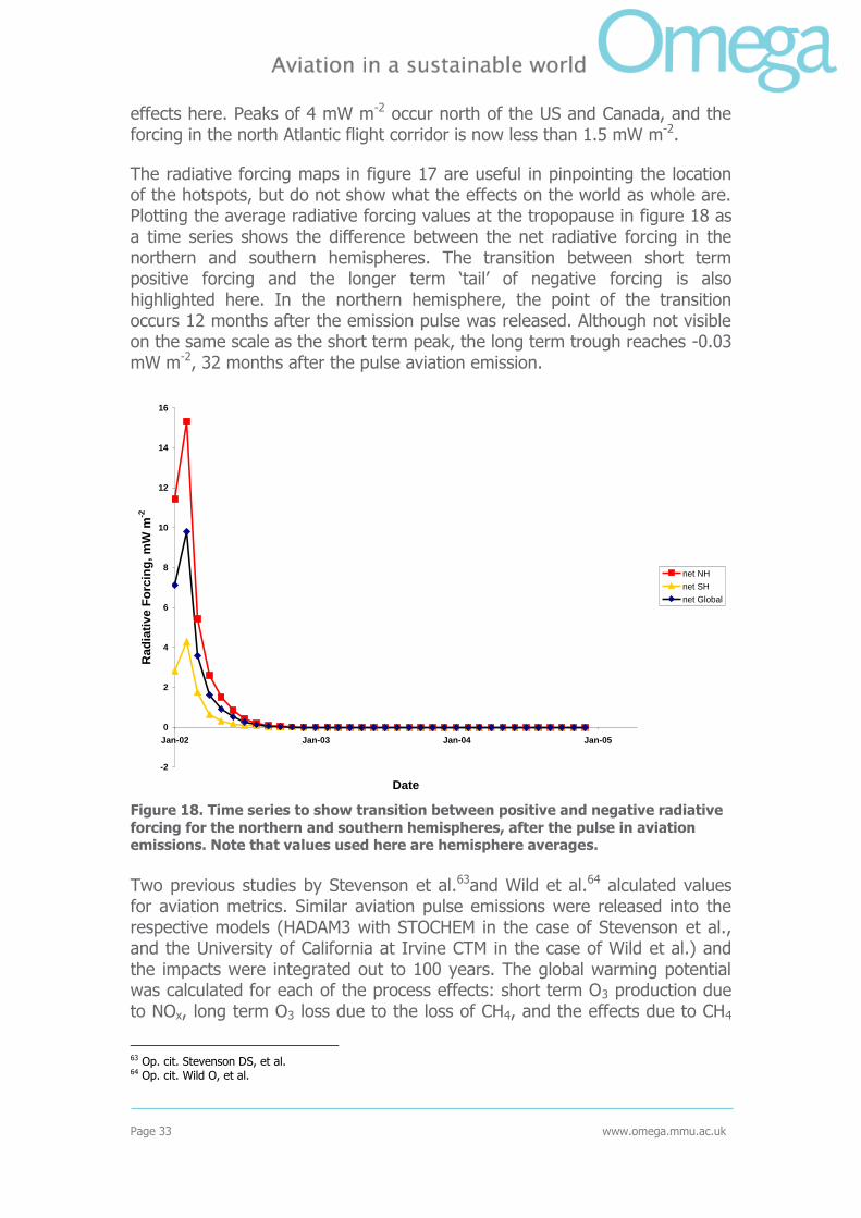
-1)-1 respectively. Clearly, there is still much uncertainty in the values for these metrics, and even differences in whether they should be positive or negative. 4.2.2 The sustained experiment Figure 19 shows the atmospheric burdens of the NOx emission and those of the subsequent degradation products of O3, CH4 and HOx (=OH+HO2). The continual input of aviation NOx ensures that the concentration of O3 is kept „topped up‟. This in turn means that there is no limit to the extent to which the CH4 burden can be reduced by.

www.omega.mmu.ac.uk

Figure 19. Time evolution of perturbations (relative to a control experiment) in the global burden of NOx, ozone, methane and HOx (=OH+HO2), for sustained

emissions of NOx as calculated in the University of Cambridge p-TOMCAT model.

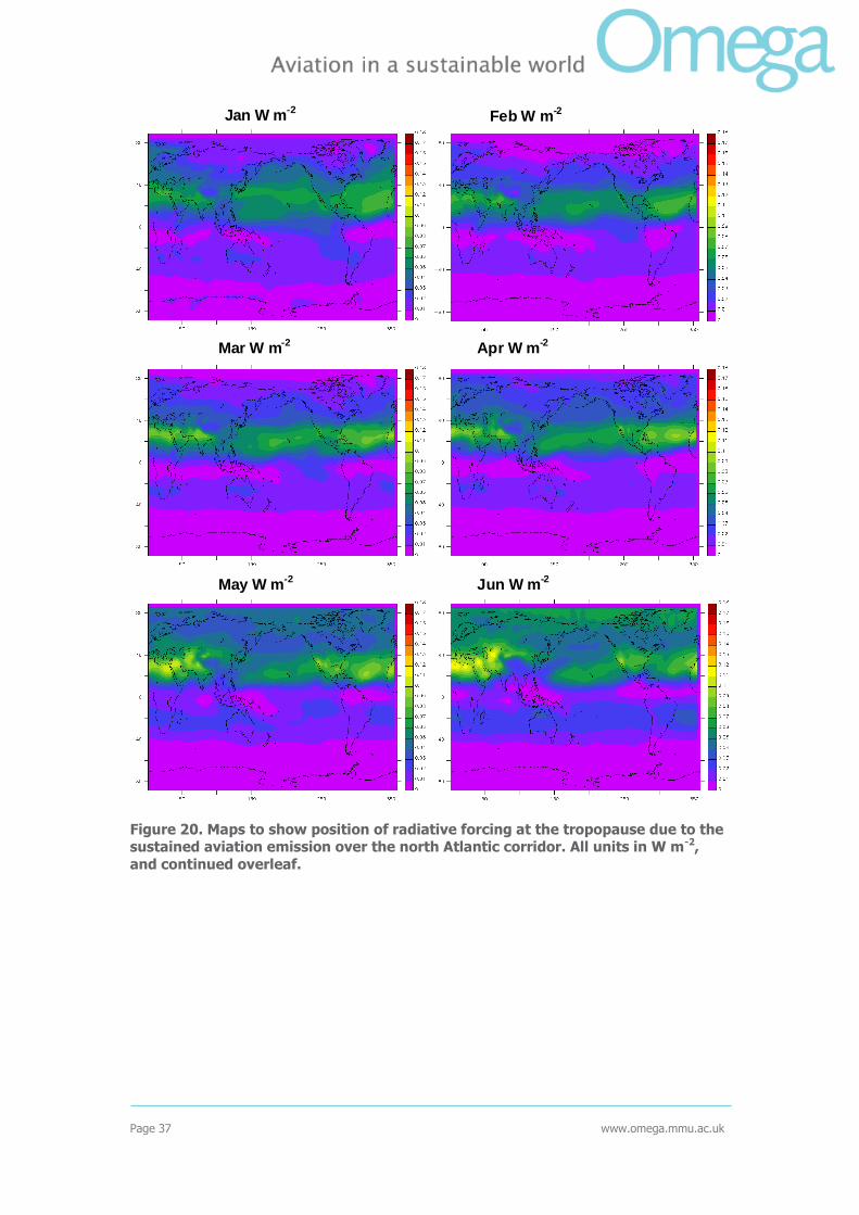
Figure 20 shows the progression of the 2.78 Tg NO2 sustained aviation experiment at the tropopause over 1 year. The legend for each of the maps is the same, unlike figure 17, as the effects of the emission, while large in magnitude, is more gradual.

www.omega.mmu.ac.uk

Jan W m-2

Feb W m-2

Mar W m-2

Apr W m-2

May W m-2

Jun W m-2

Figure 20. Maps to show position of radiative forcing at the tropopause due to the sustained aviation emission over the north Atlantic corridor. All units in W m-2,

and continued overleaf.

www.omega.mmu.ac.uk

Jul W m-2

Aug W m-2

Sep W m-2

Oct W m-2

Nov W m-2

Dec W m-2

Figure 20 continued.

Continual emissions of aviation NOx occur into the north Atlantic flight corridor in the same location as the pulse experiment. Starting in January, the peak radiative forcing again occurs in a longitudinal band between 20-40°N with a peak value of 90 mW m-2. This pattern of forcing continues for a further 4-5 months until the northern hemisphere spring-summer. By June, the peak forcing occurs over northern Africa and East Asia with values up to 130 mW m-2. This increase in positive forcing continues until the experiment maximum of 170 mW m-2 in October, after which the forcing subsides to around 90 mW m-2 until the following year. The cycle repeats with a trough between February – March and a peak around October.

www.omega.mmu.ac.uk

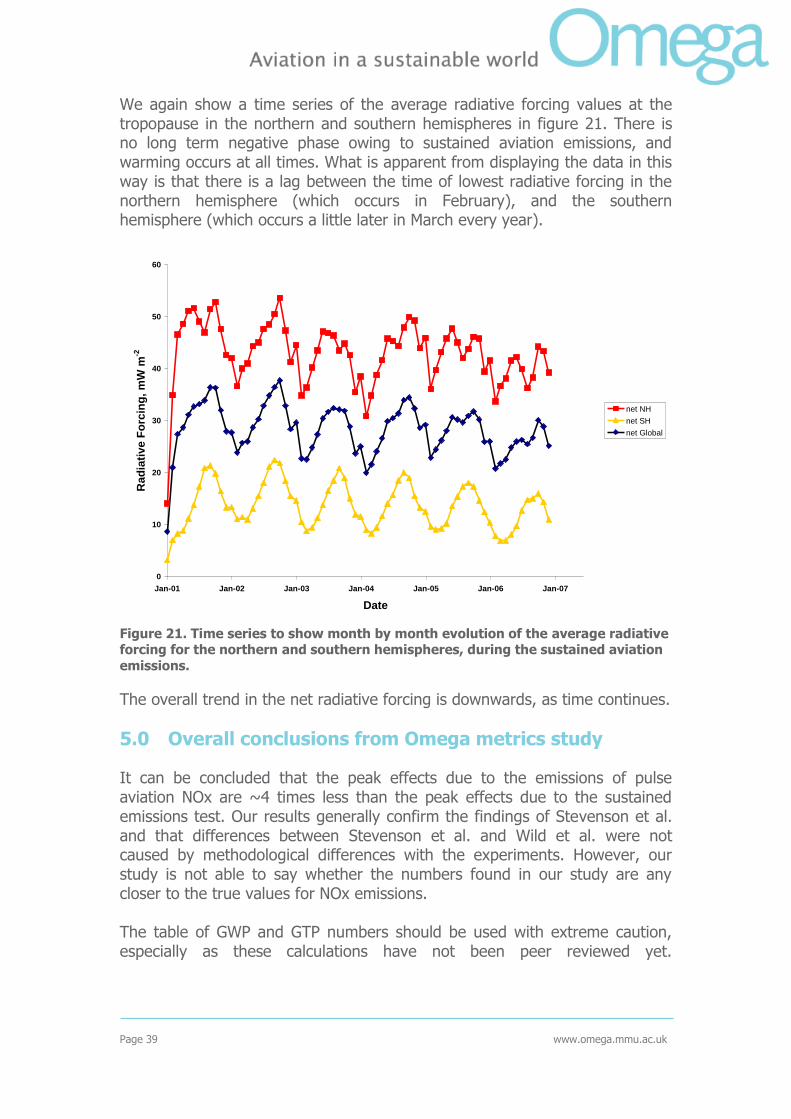
We again show a time series of the average radiative forcing values at the tropopause in the northern and southern hemispheres in figure 21. There is no long term negative phase owing to sustained aviation emissions, and warming occurs at all times. What is apparent from displaying the data in this way is that there is a lag between the time of lowest radiative forcing in the northern hemisphere (which occurs in February), and the southern hemisphere (which occurs a little later in March every year).

0

10

20

30

40

50

60

Jan-01 Jan-02 Jan-03 Jan-04 Jan-05 Jan-06 Jan-07

Date

Ra

dia

tiv

e F

orc

ing

, m

W m

-2

net NH

net SH

net Global

Figure 21. Time series to show month by month evolution of the average radiative forcing for the northern and southern hemispheres, during the sustained aviation

emissions.

The overall trend in the net radiative forcing is downwards, as time continues.

5.0 Overall conclusions from Omega metrics study

It can be concluded that the peak effects due to the emissions of pulse aviation NOx are ~4 times less than the peak effects due to the sustained emissions test. Our results generally confirm the findings of Stevenson et al. and that differences between Stevenson et al. and Wild et al. were not caused by methodological differences with the experiments. However, our study is not able to say whether the numbers found in our study are any closer to the true values for NOx emissions. The table of GWP and GTP numbers should be used with extreme caution, especially as these calculations have not been peer reviewed yet.

www.omega.mmu.ac.uk

Uncertainties should always be considered and a range of timeframes chosen in order that interpretations remain unbiased. The MAGIC study shows that for realistic scenarios of future greenhouse gas emissions. 100 year multiplies based on GWP or GTP concepts have considerable uncertainty ranges. For target approaches the multiplier increases rapidly as the cut-off date nears, as short-lived species become more important mitigation options.

6.0 References

Berntsen TK, et al., Climate response to regional emissions of ozone precursors; sensitivities

and warming potentials. Tellus 2005, 57:283-304

Borken, J., H. Steller, T. Meretei and F. Vanhove, Global and country inventory of road passenger and freight transportation – Their fuel consumption and their emissions of air

pollutants in the year 2000, Transportation Research Records, Journal of the Transportation

Research Board, 2011, 127-136, 2007.

Brunner, D., J. Staehelin, H. L. Rogers, M. O. Koehler, J. Pyle, et al., An evaluation of the performance of chemitry transport models by comparison with research aircraft observations,

1, concept and overall model performance, Atmos. Chem. Phys., 3, 1609-1631, 2003.

Brunner, D., J. Staehelin, H. L. Rogers, M. O. Koehler, J. Pyle, et al., An evaluation of the

performance of chemitry transport models by comparison with research aircraft observations, 2, detailed comparison with two selected campaigns, Atmos. Chem. Phys., 5, 107-129, 2005.

Carver, G., P. Brown and O. Wild, The ASAD Atmospheric Chemistry Integration Package and

Chemical Reaction Database, Comp. Physics Communications, 105, 197-215, 1997.

Derwent, R.G., et al., Transient behaviour of tropospheric ozone precursors in a global 3-D

CTM and their indirect greenhouse effects. Climatic Change, 2001. 49: p. 463-487.

Ehhalt, D., et al., Atmospheric Chemistry and Greenhouse Gases, in Climate Change 2001: The Scientific Basis, J. Houghton, et al., Editors. 2001, Cambridge University Press:

Cambridge, UK. p. 892.

Endresen, O., E. Sorgard, H. Behrens, P. Brett and I. Isaksen: A historical reconstruction of

ships‟ fuel consumption and emissions, J. Geophys. Res., 112, 2007.

Forster, PMdeF et al. 2007. A calculated Risk? Blue Skies magazine. The parliamentary

Monitor. 1

Forster PMdeF, et al., It is premature to include non-CO2 effects of aviation in emission trading schemes. Atmospheric Environment, 2006, doi 10.1016/j.atmosenv.2005.11.005

Forster PMdeF, et al., Corrigendum to "It is premature to include non-CO2 effects of aviation in emission trading schemes". Atmospheric Environment, 2007

doi:10.1016/j.atmosenv.2005.11.081

www.omega.mmu.ac.uk

Forster P, et al., Changes in Atmospheric Constituents and in Radiative Forcing. In: Climate

Change 2007: The Physical Science Basis. Contribution of Working Group I to the Fourth Assessment Report of the Intergovernmental Panel on Climate Change [Solomon S, Qin D,

Manning M, Chen Z , Marquis M, Averyt KB, Tignor M, Miller HL (eds.)]. Cambridge University Press, Cambridge, United Kingdom and New York, NY, USA. 2007.

Forster, P, and Rogers, H. Metrics for comparison of climate impacts from well mixed greenhouse gases and inhomogeneous forcing such as those from UTRLS ozone, contrails

and contrail cirrus. 2008

Fuglestvedt, J.S., et al., Metrics of climate change: assessing radiative forcing and emission indices. Climatic Change, 2003. 58: p. 267-331.

Fuglestvedt, J.S., et al., Climate forcing from the transport sectors. Proceedings of the National Academy of Sciences of the United States of America, 2008. 105: p. 454-458.

Friedlingstein, P., et al., Climate-Carbon Cycle Feedback Analysis: Results from the C4MIP

Model Intercomparison. Journal of Climate, 2006. 19: p. 3337-3353.

Gauss, M., et al., Impact of aircraft NOx emissions on the atmosphere – tradeoffs to reduce

the impact. Atmospheric Chemistry and Physics, 2006. 6: p. 1529.

Hansen, J., et al., Efficacy of climate forcings. Journal of Geophysical Research, 2005. 110: p. D18104.

Hoor, P., J. Borken-Kleefeld, D. Caro, O. Dessens, O. Endresen, M. Gauss, V. Grewe, D. Hauglustaine, I.S.A. Isaksen, P. Jökel, J. Lelieved, M. Meijer, D. Olivie, M. Prather, C. Schnadt

Poberaj, J. Staehelin, Q. Tang, J. van Aardenne, P. van Velthoven and R. Saussen, The impact of traffic emissions on atmospheric ozone and OH: results from QUANTIFY, Atmos.

Chem. Phys. Discuss., 8, 18219-18266,2008.

IPCC. Climate Change. The IPCC Scientific Assessment, Intergovernmental Panel on Climate

Change, Cambridge University Press, UK. 1990.

IPCC. Aviation and the Global Atmosphere, A Special Report of IPCC (Intergovernmental

Panel on Climate Change), Cambridge University Press, Cambridge, UK. 1999.

IPCC, Climate Change 2001, The Scientific Basis. Intergovernmental Panel on Climate Change, Cambridge University Press, UK, 2001.

Law, K. and E. Nisbet, Sensitivity of the methane growth rate to changes in methane

emissions from natural gas and coal, J. Geophys. Res., 101, 14387-14397, 1996.

Lee, D., B. Owen, C. Fishter, L. Lim, and D. Dimitriu, Allocation of international aviation

emissions from scheduled air traffic – present day and historical (report 2 of 3), Manchester Metropolitan University, CATE-2005-3[c]-2, Manchester, UK.

Mannstein, H. and U. Schumann, Aircraft induced contrail cirrus over Europe. Meteorologische Zeitschrift, 2005. 14: p. 549-554.

Meinshausen, M., et al., Multi-gas emission pathways to meet arbitrary climate targets.

Climatic Change, 2006. 75(1-2): p. 151-194.

Mannstein, H. and U. Schumann, Aircraft induced contrail cirrus over Europe. Meteorologische Zeitschrift, 2007. 16: p. 131-132.

www.omega.mmu.ac.uk

Meinshausen, M. and S. Raper, The rising effect of aviation on climate. Nature Geoscience

(submitted), 2008.

Meinshausen, M., et al., The emission budget for staying below 2°C global warming. (to be submitted), 2008.

Meinshausen, M., S. Raper, and T. Wigley, Emulating IPCC AR4 atmosphere-ocean and carbon cycle models for projecting global-mean, hemispheric and land/ocean temperatures.

Atmospheric Chemistry and Physics Discussions, 2008. 8: p. 6153–6272.

Meinshausen, M. et al. (2008) The emission budget for staying below 2°C global warming. Submitted to Nature.

Nakicenovic, N. and R. Swart, Eds. (2000). IPCC Special Report on Emissions Scenarios. Cambridge, United Kingdom, Cambridge University Press

O‟Connor, F., G. Carver, N. Savage, J. Pyle, J. Methven, S. Arnold, K. Dewey and j. Kent,

Comparison and visualisation of high-resolution transport modelling with aircraft

measurements, Atm. Sci. Lett., 6, 164-170, 2005.

Ponater, M., et al., On contrail climate sensitivity. Geophysical Research Letters, 2005(32).

Prather, M., Numerical advection by conservation of second-order moments, J. Geophys. Res., 91, 6671-6681, 1986.

Sausen R, et al., A diagnostic study of the global distribution of contrails Part 1: Present day climate. Theor. Appl. Climatol. 1998. 61:127-141

Sausen, R., et al., Aviation radiative forcing in 2000: An update on IPCC (1999).

Meteorologische Zeitschrift, 2005. 14(4): p. 555-561.

Savage, N., K. Law, J. Pyle, A. Richter, H. Nüss and J. Burrows, Using GOME NO2 satellite

data to examine regional differences in TOMCAT model performance, Atmos. Chem. Phys., 4, 1895-1912, 2004.

Shine, K.P., et al., Alternatives to the global-warming potential for comparing climate impacts of emissions of greenhouse gases. Climatic Change, 2005. 68: p. 281-302.

Shine KP, et al., Comparing the climate effect of emissions of short- and long-lived climate

agents. Accepted for publication in Phil. Trans. R.Soc. 2007.

Stevenson DS, et al., Radiative forcing from aircraft NOx emissions: mechanisms and

seasonal dependence. Journal of Geophysical Research 2004, 109:D17307

Svensson F, et al., Reduced environmental impact by lowered cruise altitude for liquid hydrogen-fuelled aircraft. Aerospace Science and Technology, 2004, 8:307-320

Tiedtke, M, A comprehensive mass flux scheme for cumulus parameterisation on large scale models, Mon. Weather Rev., 117, 1779-1800, 1989.

Trudinger, C. and I. Enting, Comparison of formalisms for attributing responsibility for climate

change: Non-linearities in the Brazilian proposal approach. Climatic Change, 2005. 68: p. 67-99.

Wild O, et al., Indirect long-term global radiative cooling from NOx emissions. Geophysical Research Letters 2001, 28:1719-1722

www.omega.mmu.ac.uk

Wit RCN, et al., Giving wings to emission trading. Inclusion of aviation under the European emission trading system (ETS): design and impacts. CE-Delft, No. ENC.C.2/ETU/2004/0074r,

the Netherlands. 2005.

7.0 Appendix The description below of MAGICC 6.0 and its adaptations to take into account the climate effects of aircraft emissions were largely adopted from Meinshausen and Raper67. General description of the model setup for aviation experiments MAGICC 6.0 was set up to emulate 10 carbon-cycle models that participated in the C4MIP inter-comparison project68, and employ other gas-cycle parameterisations and radiative forcings in line with IPCC‟s Fourth Assessment Report AR469. These forcings include climate feedbacks and depend therefore on the attendant temperature changes. We have adapted the MAGICC model to account for high-altitude NOx emissions and their higher efficiency compared to ground-based emissions in terms of increasing tropospheric ozone abundances and reducing methane lifetime. Current knowledge on contrail and aviation induced cirrus forcing is included70 71. The radiative forcing by cirrus and contrails is a relatively large part of the total aviation induced forcing, although rather uncertain. We assume a linear relationship between jet fuel use and contrails. Sooner than contrails, cirrus clouds might face saturation effects, but there is ambiguous observational evidence as to whether any saturation can be detected already72 73. Hence, we chose to employ a very wide uniform distribution for an asymptotic global limit on aviation-induced cirrus forcing. Uncertainty ranges on the core parameters in MAGICC‟s upwelling-diffusion climate module were constrained by linking of a set output variables to observations74. From the climate model, global-mean temperature changes are derived that in turn impact on the carbon-cycle and other gas-cycles in the coupled climate-carbon cycle model of the MAGICC set up. For the

67 Meinshausen, M. and S. Raper, The rising effect of aviation on climate. Nature Geoscience (submitted), 2008. 68 Friedlingstein, P., et al., Climate-Carbon Cycle Feedback Analysis: Results from the C4MIP Model Intercomparison. Journal of Climate, 2006. 19: p. 3337-3353. 69 Op. cit. Forster P, et al., 2007 70 Gauss, M., et al., Impact of aircraft NOx emissions on the atmosphere – tradeoffs to reduce the impact. Atmospheric Chemistry and Physics, 2006. 6: p. 1529. 71 Sausen, R., et al., Aviation radiative forcing in 2000: An update on IPCC (1999). Meteorologische Zeitschrift, 2005. 14(4): p. 555-561. 72 Mannstein, H. and U. Schumann, Aircraft induced contrail cirrus over Europe. Meteorologische Zeitschrift, 2005. 14: p. 549-554. 73 Mannstein, H. and U. Schumann, Aircraft induced contrail cirrus over Europe. Meteorologische Zeitschrift, 2007. 16: p. 131-132. 74 Meinshausen, M., et al., The emission budget for staying below 2°C global warming. (to be submitted), 2008.

www.omega.mmu.ac.uk

simulations, we drew 1500 parameter sets for tropospheric ozone and methane forcing efficiencies from IPCC AR4 conforming prior distributions, and combined them with parameter distributions emulating literature estimates for NOx, contrail, cirrus and H2O induced effects. These parameters sets were then combined at random with C4MIP model emulations and observationally-constrained prior distributions for the climate-model parameters, while other parameters were set to best guess IPCC AR4 values. There are multiple non-linearities in the radiative forcing calculations, which is why we use the residual method to estimate sectoral contributions to forcing and temperatures75. The tropospheric ozone and methane gas cycle parameterizations within MAGICC 6.0 are amended in order to account for the difference in effects of ground-based and high-altitude NOx emissions. A calibration to published pulse response experiments of chemical transport models76 77 78, yields substantially lower enhancement factors compared to a calibration to year 2000 values as presented in the literature79 80. In order to more closely emulate current knowledge on the overall effect of NOx emissions, and thereby minimizing the effect of potential non-lineararities, we use the latter method. Distributions for the enhancement factors βO3 and βCH4 are calibrated using 1000-member runs drawn at random from multiple parameter distributions. A key assumption is that the – relatively large - overall tropospheric ozone forcing uncertainty provided by IPCC81 with a likely range between 0.25 and +0.65 W.m-2 contributes proportionally to the aviation share of induced tropospheric ozone forcing. The aviation-induced tropospheric ozone forcing is hence considered to be the compound of the overall tropospheric ozone uncertainty and an uncertainty in the effectiveness of aviation NOX emissions. For methane, the total forcing uncertainty is relatively small (+0.48 ± 0.05 W.m-2) and we assume the uncertainty of aviation-induced CH4 forcing is fully represented by the effectiveness of aviation NOX on the CH4 lifetime. The distributions for β are chosen, so that log(β-c) has a Gaussian distribution with c being a constant to determine the skewness of the distribution. The

two parameters of the Gaussian distribution, mean, , and variance, 2 , and the skewness parameter, c, are then selected to match the provided median and lower and upper bound of the distribution range from the literature. 75 Trudinger, C. and I. Enting, Comparison of formalisms for attributing responsibility for climate change: Non-linearities in the Brazilian proposal approach. Climatic Change, 2005. 68: p. 67-99. 76 Op. cit. Stevenson DS et al 77 Op. cit. Wild O, et al 78 Derwent, R.G., et al., Transient behaviour of tropospheric ozone precursors in a global 3-D CTM and their indirect greenhouse effects. Climatic Change, 2001. 49: p. 463-487. 79 Op. cit. Gauss, M., et al. 80 Fuglestvedt, J.S., et al., Climate forcing from the transport sectors. Proceedings of the National Academy of Sciences of the United States of America, 2008. 105: p. 454-458. 81 Op. cit. Forster P, et al., 2007

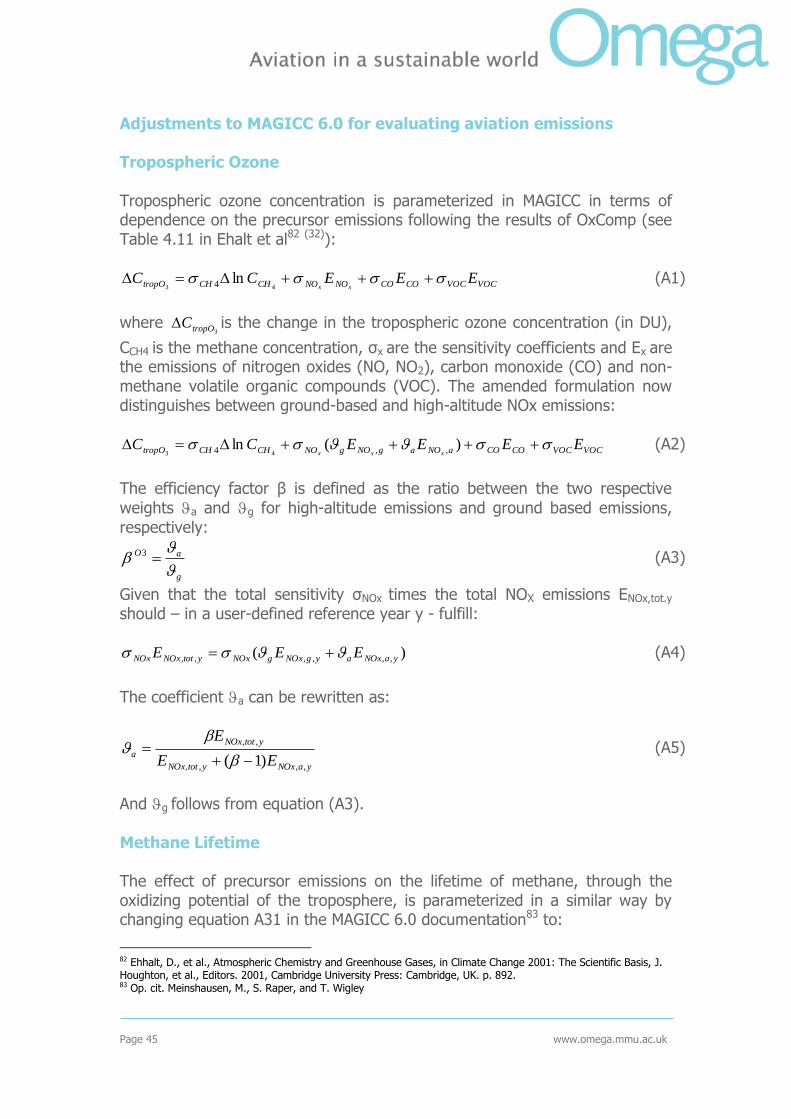
www.omega.mmu.ac.uk

Adjustments to MAGICC 6.0 for evaluating aviation emissions Tropospheric Ozone Tropospheric ozone concentration is parameterized in MAGICC in terms of dependence on the precursor emissions following the results of OxComp (see Table 4.11 in Ehalt et al82 (32)):

VOCVOCCOCONONOCHCHtropO EEECCxx

43

ln4 (A1)

where

3tropOC is the change in the tropospheric ozone concentration (in DU),

CCH4 is the methane concentration, σx are the sensitivity coefficients and Ex are the emissions of nitrogen oxides (NO, NO2), carbon monoxide (CO) and non-methane volatile organic compounds (VOC). The amended formulation now distinguishes between ground-based and high-altitude NOx emissions:

VOCVOCCOCOaNOagNOgNOCHCHtropO EEEECCxxx

)(ln ,,4 43 (A2)

The efficiency factor β is defined as the ratio between the two respective

weights a and g for high-altitude emissions and ground based emissions,

respectively:

g

aO

3 (A3)

Given that the total sensitivity σNOx times the total NOX emissions ENOx,tot.y should – in a user-defined reference year y - fulfill:

)( ,,,,,, yaNOxaygNOxgNOxytotNOxNOx EEE (A4)

The coefficient a can be rewritten as:

yaNOxytotNOx

ytotNOx

aEE

E

,,,,

,,

)1(

(A5)

And g follows from equation (A3).

Methane Lifetime The effect of precursor emissions on the lifetime of methane, through the oxidizing potential of the troposphere, is parameterized in a similar way by changing equation A31 in the MAGICC 6.0 documentation83 to:

82 Ehhalt, D., et al., Atmospheric Chemistry and Greenhouse Gases, in Climate Change 2001: The Scientific Basis, J. Houghton, et al., Editors. 2001, Cambridge University Press: Cambridge, UK. p. 892. 83 Op. cit. Meinshausen, M., S. Raper, and T. Wigley

www.omega.mmu.ac.uk

VOC

OH

VOCCO

OH

COaNO

OH

agNO

OH

g

OH

NOCH

OH

CHOH EEEECAxxx

)(ln)ln( ,,4 4 (A6)

Where AOH is the tropospheric OH abundance, and OH

x are the sensitivity

coefficients for the influence on OH of CH4, NOx, CO and VOC, respectively.

The coefficients OH

a and OH

g are the weights on high-altitude and ground-

based emissions, respectively, with their ratio indicated by βCH4. Methane‟s lifetime is then adjusted according to:

))ln(exp(0

OHA (A7)

where τ0 and τ are the methane lifetimes before and after accounting for changes in the oxidizing potential of the troposphere (see section A2.1 in Meinshausen et al84). Radiative Forcing Aircraft-Induced Cirrus Clouds Cirrus forcing Fcirrus at time t is approximated by:

))'

)(exp(1()(

Fuel

tFuelFtF pot

cirruscirrus (A8)

Where Fuel(t) indicates aviation fuel consumption, Fuel‟ is the consumption

level at which the forcing limit is approached up to (1-1/e) pot

cirrusF , and the

asymptotic radiative forcing limit pot

cirrusF is defined as a multiple α of the year

2000 forcing:

)2000(cirrus

pot

cirrus FF (A9)

Given that equation A8 must hold for year 2000 conditions, Fuel‟ can be derived as:

)1ln()ln(

)2000('

FuelFuel (A10)

Calibration to NOx pulse emission studies We closely replicate the experimental set-up of pulse emission studies85 86 87 in order to calibrate efficiency factors for high-altitude NOx emissions. For the background scenario, MAGICC was run from 1765 to 1990 with historical anthropogenic emissions and thereafter emissions were kept constant at 1990

84 Op. cit. Meinshausen, M., S. Raper, and T. Wigley 85 Op. cit. Stevenson DS et al 86 Op. cit. Wild O, et al 87 Op. cit. Trudinger, C. and I. Enting

www.omega.mmu.ac.uk

levels. In 1991, a 1TgNOx pulse emission was added. The high-altitude efficiency factor βO3 was then calibrated so that the 100-year integrated tropospheric ozone radiative forcing perturbation matched the short and long-term effect indicated by the CTM studies. Similarly, the 100-year integrated change in methane concentrations was matched by adjusting the efficiency factor βCH4. In order to match these idealized pulse experiment studies optimally, the calibration routine suggests that high-altitude NOx emissions should be considered 4.0 to 7.1 times more effective in terms of inducing tropospheric ozone increases and 4.3 to 4.7 times more effective in terms of reducing methane‟s lifetime and consequently methane concentrations. See Table A.1 for results.

Figure A.1 - Calibration of tropospheric ozone and methane lifetime effects to a 1

Tg NOx pulse emission

In an alternative method to calibrate the high-altitude NOx efficiency factor, we ran our model with historical aviation emission time series using Monte Carlo simulations as described below (see Table A.2) and adjust the NOx efficiency factor so that we approximately match the results of recent literature estimates for aviation-NOx induced tropospheric ozone forcing and methane forcing anomalies in year 200088 89. Table A.1 - Calibration of efficiency factors for high-altitude NOx emissions versus

ground-based NOx emissions with respect to their effect on tropospheric ozone

and methane.

88 Op.cit. Gauss, M., et al., 89 Op.cit. Fuglestvedt, J.S., et al., 2008

www.omega.mmu.ac.uk

Trop. O3 (Short + Long Term) CH4

Calibrated Study

Original (mW/m2*yrs)

Calibrated Value

(mW/m2*yrs)

Calibration Factor βO3 (Efficiency

NOxair/ NOxground)

Original (ppb*yrs)

Calibrated Value

(ppb*yrs)

Calibration Factor βCH4 (Efficiency

NOxair/ NOxground)

Pulse Experiment 1 Tg NOx in 1990 background conditions, integrated over 100 yrs

Derwent et al. (as presented in Stevenson et al.)

7.90 (=8.6-0.7) 7.90 7.137 -12.5 -12.5 4.700

Wild et al (as presented in Stevenson et al.)

6.40(=7.9-1.5) 6.40 5.937 -12.2 -12.2 4.602

Stevenson et al.

4.11(=5.06-0.95)

4.11 4.073 -11.3 -11.3 4.283

Time-Slice 2000 Experiment with full all-gas aviation history.

Gauss et al. as applied in Fuglestvedt et

al.

22 (-11, +22) 21(-11, +30) 10.27

(6.27 to 17.57) 68.26% range

-10(-21, +7) mW/m2

-9 (-23, +6) mW/m2

8.13 (2.13 to 42.5) 68.26%

Monte-Carlo Climate Simulations

Assuming independence between carbon cycle, climate response, and some individual radiative forcing parameter uncertainties, we employ a 1500-member Monte Carlo simulation. For carbon cycle uncertainties, emulations of 10 C4MIP carbon cycle models90 are employed at random. Climate response uncertainties are taken into account by randomly selecting parameter sets from a series of parameter sets that were constrained by observations of key output variables91. The a priori distributions for non-CO2 forcing parameters, namely the radiative efficiency of tropospheric ozone, methane, nitrous oxide, direct sulphate, black carbon, and organic carbon, are chosen so that the global emission history92 results in year 2005 forcing distributions that match those detailed in IPCC AR4, Table 2.1293. Despite large uncertainties in the indirect aerosol effects, they are not varied, but kept at their IPCC AR4 best estimate values, as an assumption of independence between this strong negative forcing and climate response is not justified. This is because, for example, a high aerosol cooling implies a small overall anthropogenic

90 Op.cit. Meinshausen, M., S. Raper, and T. Wigley 91 Meinshausen, M., et al., The emission budget for staying below 2°C global warming. (to be submitted), 2008. 92 Op.cit. Meinshausen, M., S. Raper, and T. Wigley 93 Op. cit. Forster P, et al., 2007

www.omega.mmu.ac.uk

radiative forcing over the last century. This would necessitate assuming high climate sensitivity in order to match the observed historical temperature evolution. For all chosen priors see Table A.2. Table A.2 - Chosen prior distributions for 1500-member Monte Carlo simulations Parameter (sets) Description Chosen prior

Source

18 Carbon Cycle parameters

Eighteen MAGICC 6.0 carbon cycle parameters were tuned to optimally match detailed carbon cycle characteristics of the C4MIP models (23).

Ten parameter sets representing the C4MIP carbon cycle models (19).

MAGICC 6.0 documentation

82 Climate Response parameters

82 MAGICC 6.0 climate module parameters were tuned to

optimally match selected output variables with historical records of observational constraints

500 parameter sets from observational

constraining

Meinshausen et al 94

βO3 - AIR_TROPOZ_NOXAIR_SCALE

High-altitude NOX efficiency on trop. Ozone (Ratio)

10.27 (68% range: 6.27 17.57); skewed normal‡

This study‟s calibration towards literature studies

βCH4 - AIR_CH4_NOXAIR_SCALE

High-altitude NOX efficiency on methane lifetime (Ratio)

8.13 (68% range: 2.13 to 42.5); skewed normal‡

See above.

TROPOZ_RADEFF_WM2PERDU

Radiative efficiency of tropospheric ozone (W/m2/DU) in order to match IPCC AR4 estimate, IPCC AR4 WG1 Table 2.12


This study‟s calibration to IPCC AR4

CH4_RADEFF_WM2PERPPB

Radiative efficiency of methane forcing (W/m2/ppb) in order to match IPCC AR4 estimate, IPCC AR4 WG1 Table 2.12


See above.

RF_SOXI_DIR_WM2 Direct radiative forcing of sulphate aerosols in year 2005 (W/m2) in order to match IPCC AR4 estimate, IPCC AR4 WG1 Table 2.12

-0.4 (90% range -0.2 to -0.6); skewed normal‡

See above.

RF_BCI_DIR_WM2 Direct forcing of industrial black carbon emissions in year 2005 (W/m2) in order to match IPCC AR4 estimate, IPCC AR4 WG1 Table 2.12


See above.

RF_AIR_H2O_WM2 Radiative forcing of aviation induced stratospheric water-

vapour in year 2005 (W/m2)

0.002 (68% range: 0.001 to 0.007);

skewed normal‡

Table 5 in Fuglestvedt et al.

RF_AIR_CONTRAIL_WM2

Radiative forcing of aviation induced linear contrails in year 2005 (W/m2)



RF_AIR_CIRRUS_WM2

Radiative forcing of aviation induced cirrus in year 2005 (W/m2)



RF_AIR_CIRRUS_SCALEYR2MAX

Asymptotic limit on cirrus forcing as multiple of year 2000 forcing (Factor)

5 to 30; uniform distribution

This study‟s assumption to reflect potential saturation effects.

All other parameters MAGICC 6.0 default settings based on IPCC AR4

No distribution – default settings.

MAGICC 6.0 documentation

94 Meinshausen, M. et al. (2008) The emission budget for staying below 2°C global warming. Submitted to Nature.

www.omega.mmu.ac.uk

For the efficacies of radiative forcings, i.e. their efficiency per unit radiative forcing to change surface temperatures compared to a unit forcing by CO2

95 ,

we used default settings as specified in the supplementary material of 96. For the aviation specific forcings of contrail and induced cirrus, we choose an efficacy of 0.6, following Ponater et al.97

95 Hansen, J., et al., Efficacy of climate forcings. Journal of Geophysical Research, 2005. 110: p. D18104. 96 Op.cit. Ponater, M., et al 97 Op.cit. Ponater, M., et al

omega metrics – final report - centre for aviation transport and

Documents