1

Oligopoly and Trade: What, How Much, and For Whom?

Roy J. Ruffin1

January 1999

This paper integrates the Cournot oligopoly model with the Ricardian comparative advantagemodel under conditions of Mill-Graham demand. The Ricardian trade pattern is robust, but can bereversed in extreme conditions with small enough differences in comparative advantage. Trade volumeincreases substantially with increases in competition in world export industries. There is a threshold levelof competition that creates world economic efficiency. When competition is less than the threshold level,workers gain substantially and capitalists generally lose from trade; when competition is greater than thethreshold level, both workers gain and capitalists generally gain. The folk theorem that the gains fromtrade for the economy exceed competitive gains does not hold when export competition is less than thethreshold level.

Concern over the issue of oligopoly has inspired a voluminous body of research in the trade

literature. While oligopoly may not be ubiquitous, as persuasively argued by Clair Wilcox in a classic

article (Wilcox, 1950), the existence of persistent above-average profits in industries such as

pharmaceuticals, tobacco, and technology raises questions about its role in international trade (Mueller,

1986).2 Moreover, a casual perusal of American industrial structure suggests that on the average there may

be more oligopoly power, as measured by domestic measures of concentration, in the export-oriented

sectors than in the import-competing sectors. Indeed, we also have it on the authority of the Justice

Department that Intel and Microsoft are monopolies!3 How much difference does it make if oligopoly

power differs between sectors? What is the role of persistent profits? What is traded, how much is traded,

and who gains from trade? These questions can only be answered in the context of a general equilibrium

model.

This paper assumes a Cournot oligopoly in each sector of a Ricardian model of comparative

advantage in the tradition represented by the Dixit-Stiglitz-Krugman model of monopolistic competition

(Dixit and Stiglitz 1977; Krugman, 1979). This tradition is to use a utility function that lends itself to

general equilibrium analysis. Previous attempts by Fisher (1988) and Cordella and Gabszewicz (1997)

have assumed that oligopolistic firms maximize utility within the context of a single worker manager facing

a Ricardian technology. Monopoly power or oligopoly has been assumed in one industry and perfect

competition in the other industry or industries (Markusen, 1981; Kemp and Okawa, 1995). Of course, the

majority of applications of the Cournot model to international trade have been partial equilibrium (Brander,

1981; Brander and Krugman, 1983; Venables, 1985; Helpman and Krugman, 1986).4

2

This paper takes advantage of a nice property of a Cournot oligopoly facing a unit elastic demand

function: the price of the product equals the sum of all active firms’ marginal costs divided by the number

of firms minus one. The great advantage of my formulation is that it is analytically tractable and leads to

some new insights into the importance of market structure. The old insights are reprised in a general

equilibrium framework. The conclusion of Helpman and Krugman (1986, p 261) that in the presence of

imperfect competition “comparative advantage is alive and well” is confirmed. I shall show that oligopoly

does little to dim the light of Ricardian comparative advantage. Somewhat rarely, in the free trade

equilibrium the no-trade outcome is possible but with significant gains from trade due to the increase in

competition (Markusen, 1981). The new insights come from a concept I call the threshold level of

competition in the world export industries. This threshold level determines not only whether world

economic efficiency obtains, but also the extent of the gains from trade for the economy, workers, and

capitalists. I show that when the level of competition falls short of the threshold level, workers gain and

capitalists lose from international trade. When the level of competition exceeds or equals the threshold

level, workers gain and capitalists will gain in most circumstances. Helpman and Krugman (1986, p. 96)

present what might be called the folk theorem that under oligopoly the gains from trade are greater than in

the competitive case, since there is a pro-competitive effect from international trade. I will show that this

only holds in a special case and that when there is genuine oligopolistic competition across borders this

claim is generally false. Finally, the volume of international trade is highly sensitive to the amount of

oligopoly: economy-wide reductions in concentration, brought about for example by deregulation, should

increase the volume of trade substantially. These results are all conducted under the special case of a Mill-

Graham demand function, which allows us to calculate a Nash equilibrium and by the hand of providence

leads to incredibly simple solutions for the symmetrical case.

The intuition of the model suggests that the special demand assumptions only affects the

quantitative and not the qualitative nature of the results because they depend on the fundamental features of

oligopoly. The first feature is that due to entry limitations oligopoly profits are persistent; the second is that

more competition will lower price and drive out of business the higher cost firms. The hallmark of

Ricardian trade theory is that costs differ across countries. This is why in a large country there must be a

threshold level of competition in the Ricardian natural export industry that will drive out the potential

3

competitors in the other country. If in autarky the natural export industry of a country has high persistent

profits, that is, very little competition, the opening of trade may not serve to drive the high cost foreign

producer out of business (as in the Ricardian model). Thus, with limited competition, the move from

autarky to free trade can drive down oligopoly profits because everyone in the world is facing more

competition. Workers will benefit tremendously from this move because prices will drop from the pro-

competitive effect in all industries. On the other hand, if in autarky the natural export industries are very

competitive, so oligopoly profits are low to begin with, the opening of trade can wipe out the foreign

competition because their cost disadvantage is not protected by high oligopoly prices in the world’s natural

export industries. Thus, when trade is opened, and the natural export industries are competitive to begin

with, the profits of the natural export industries will soar because they will gain the entire world market.

Since natural export industries are likely to earn more profits in autarky than natural import industries,

profits as a whole rise. Workers still gain because import prices fall just as in the standard Ricardian

model. When competition exceeds the threshold level, the volume and pattern of trade are Ricardian.

When competition falls short of the threshold levels, trade patterns are in the majority of cases the same as

Ricardo but the volume is much less. It should be clear from this intuition that the results of the paper will

generalize to broader settings.

Since free trade increases profits when domestic competition is strong and lowers profits when

domestic competition is weak (for large countries), the paper suggests the hypothesis that free trade may

cause stock market booms or busts, depending on the state of domestic entry conditions in their natural

export industries. Thus, the paper gives a highly tentative and undoubtedly partial explanation of the stock

market boom in the U.S. and the long bear market in Japan: both result from freer world trade. Similarly,

in a world of weak oligopolies, protectionism (as with the Smoot-Hawley tariff of 1930), would cause stock

market collapses.

Section I reviews the essential results from Cournot oligopoly. Section II presents the general

equilibrium analysis of a single country. Section III examines the two-country case for the non-

symmetrical and symmetrical cases. Section IV is devoted to the gains from trade. Finally, Section V

states the conclusions.

I. Cournot Oligopoly: Partial Equilibrium

4

This section shows that a Cournot oligopoly facing a unit elastic demand function has a simple

solution useful to trade theorists. Let xj denote the output of firm j and Q the output of the industry.

Clearly, Q =∑ xj Let cj denote the constant marginal cost of production for the jth firm. A Cournot

oligopoly consists of N firms producing a homogeneous product in which each firm knows the market

demand function P = P(Q) and assumes all other firms continue to produce their current outputs. Then the

Cournot equilibrium is defined by:

(1) P(Q) + P’(Q)xj = cj

If we sum (1) over all N firms we have

(2) NP(Q) + P’(Q)Q = ∑ cj.

It is important to use a form of the demand function that can be derived from utility maximization as well

as one that works well with Cournot oligopoly. We assume that P = AQ-1, where A is a constant that will

later reflect income, then substitution into (2) yields the simple result that

(3) P = ∑ ci/(N-1).

This result will be important in the general equilibrium section.5 If P < cj for any firm j, firm j should be

dropped and the sum in (3) recalculated. Thus, there is no free entry, but there is the possibility of exit

when profit is negative. The key property of (3) is that the price of the product does not depend on

income; this makes the result particularly useful in general equilibrium because there are no feedback

effects between income and the prices charged by the oligopolists.

We can substitute the inverse demand function into (1) to determine each firm’s output. It is

(4) xk = A(P – ck)/P2

Thus, it is very easy to deal with the case of firms producing with different costs, since each firm’s output

bears the same proportion to its profit margin. This is ideal for the Ricardian model, because the cost of

any good is higher in the country with a comparative disadvantage in that good.

It is also useful to note that the Herfindahl index of concentration, H = ∑ (xj/Q)2 , is proportional to

aggregate profit. From (4), the profit of firm k is simply

(5) Πk = A(P-ck)2/P2.

However, using the demand function Q = A/P we find that xk/Q = Pxk/A. Thus, directly from (4), we have

(xk/Q) = (P-ck)/P and squaring we find from (5) that the Herfindahl index is simply:

5

(6) H = (1/A)∑ Πk .

This is useful because it shows that if free trade raises or lowers aggregate profit, it raises or lower

measured concentration in the industry.

A point that is fundamental comes directly from (3). When there is an increase in the number of

low-cost firms, the price of the good naturally falls and, in the case of heterogeneous marginal costs, it must

eventually happen that the high cost firms are driven from the market. For example, suppose it happens that

firm 5 is the highest cost firm and that P = c5 + epsilon. Clearly, if any firm with costs lower than firm 5’s

costs comes into the market, from (3) the price must fall, thus possibly causing firm 5 to exit the market.

This conclusion is important because in a Ricardian world it must be that for any good the costs of

production are higher in the country with a comparative disadvantage in that good. Whether free trade

drives such firms out of business has important ramifications independent of the specific model being used.

II. Cournot Oligopoly: Autarkic General Equilibrium

Because of the simple demand function it is easy to extend the above analysis to general

equilibrium. In general equilibrium we must justify the assumption that firms simply maximize profit. I

do so by supposing that each firm separates the prices it pays as a consumer from the prices it receives as a

producer. Several authors have assumed that the oligopolist maximizes an indirect utility function

(Cordella, 1998; Cordella and Gabszewicz, 1997; Kemp and Okawa, 1995). The purpose of this procedure

is to avoid a problem with modeling oligopoly in general equilibrium models: what is the numeraire in

which the oligopolist expresses his profit? By using the Mill-Graham utility function, in which the

equilibrium oligopoly price does not depend upon income (only the number of firms and no other

parameters) and, hence, the numeraire, I can avoid such problems. Thus, we can use the results of Section

I to examine the Ricardian trade model. .

I begin with a basic lemma that holds for an imperfectly competitive model with only one

productive factor. Assume an economy with one factor, labor, and N industries. The wage rate is w, the

output and profit of the jth industry are Qj and Πj. National income is Y = wL + ∑ Πj. However, since Πj

= (pj – waj)Qj, where aj is the familiar Ricardian labor input per unit of good j, we find that Y = wL +

∑ PjQj – w(∑ ajQj). Clearly, the sum ∑ ajQj is the demand for labor. Now for any arbitrary pattern of

outputs and wage rate, Y = ∑ PjQj implies the demand for labor equals the supply of labor. It is useful to

6

state this lemma because in the sequel we will find that the labor market clearing equation— so cherished

by trade economists--is implied in one representation of the model. Thus:

Basic Lemma: In a one-factor Ricardian model with oligopoly, for any fixed w and output pattern,

the demand for labor equals the supply of labor if and only if the value of production equals the sum of all

income payments.

Consider now an autarkic economy that produces only two goods, 1 and 2, with homogeneous

labor under constant returns to scale. Let pi = price of good i and w = wage rate. We shall assume that

labor is the numeraire (w = 1), but it makes no difference in this model. We designate by t = p1/p2, the

commodity terms of trade of good 2 for good 1. I will assume the useful Mill-Graham utility function U

= (C1 ,C2 ).5. No insights arise from any additional generality purchased by assuming a more general Cobb-

Douglas utility function. 6 Thus, the demand function for good i is Di = Y/2pi, where Y is income. Let Nj

denote the actual number of firms in industry j.

The profit margin in industry i is Mi = pi – wai = pi – ai, using the numeraire w = 1. The pricing

equations flow from equation (3) above:

(7) pi = Niai /(Ni-1).

Since industry profits equal the profit margin times product demand,

(8) Πi = (pi –ai)Y/2pi= MiY/2pi.

Finally, national Income is simply wages plus profits:

(9) Y = L + Π1 + Π2.

These 5 equations determine the five unknowns, p1, p2, Y, and the Πj’s. Clearly, we can solve (7) for the

pi’s and the terms of trade, t, and (8) and (9) imply that Y = 2L/(2 – M1/p1 – M2/p2 ). Recall that from the

proceeding lemma we do not need a labor-market clearing equation; this follows from (8) and (9).

The model may alternatively be depicted by proceeding directly from equation (4) in the

proceeding section. From (4) we can write Qi = YNi(Mi)/2pi2, where A=Y/2 in this case. By looking at the

ratio of industry outputs, we can eliminate Y/2 to obtain

(10) Q1/Q2= (N1M1/N2M2t2),

where you recall that t is the relative price of good 1. Clearly, from (7), we can derive the ratio of outputs

recursively. The outputs can then be determined from the standard labor market equation:

7

(11) a1Q1 + a2Q2 = L.

Thus, we have two representations of the model. Equations (7), (8), and (9) determining pi, Πi, and Y; or,

(7), (10), and (11) determining pi,and Qi .

It is clear from (7) that if N1 =N2 = N , p1/p2 = t = a1 /a2 , so that the solution is the same as in the

competitive case, except for the distribution of income between the two classes. Thus, just as also argued

by Lerner (1943):

Proposition 1 (Lerner): If N1 =N2 = N, then Pareto-efficiency obtains.

It is useful to remark that in the case of N1 = N2 = N, the autarkic levels of national income Y and

profit Π are simply Y = NL/(N-1) and Π = L/(N-1). To show this note that Y = 2p1Q1, since half of income

is spent on good 1; also half the labor force is allocated to good 1 so that Q1 = L/2a1. Noting the pricing

equation (7) shows that Y = NL/(N-1). Since wages are simply L when w = 1, Π = Y – L = L/(N-1). It

follows that the level of utility in autarky will be

(12) UA = Y/2(p1p2).5 = L/(a1a2).5

The level of utility for workers and capitalists will be

(13) UAworkerrs = L(N-1)/N(a1a2).5 and UA

capitalists = L/2N(a1a2).5.

We will have occasion to use these when we examine the gains from trade.

Finally, for the case of homothetic demands and constant returns to scale, the level of productivity

and the labor supply has a simple impact on the variables. Changing L leaves all prices intact, but simply

changes profits and total income proportionately. Replacing the labor cost coefficients by ajo = λaj leads to

the solution Yo = Y/λ, and Πjo = Πj/λ. Thus, only the ratio a1/a2 matters for questions regarding the

benefits and relative volume of exchange.

III. Cournot Oligopoly: Trade

Suppose we now have two countries— the home and the foreign. Unlike the contributions of

Brander (1981) and Brander and Krugman (1983), I assume that there is an integrated world market for

each of the goods.

Once international trade is admitted, the difference in costs between countries can lead to the shut-

down of import-competing industries. When the profit-margin is nonpositive, then the number of firms in

the domestic industry is assumed to be zero, and no resources are absorbed by such a shut-down. This is a

8

standard feature of Arrow-Debreu-McKenzie general equilibrium models in which firms do not themselves

absorb (but merely use) resources. Thus, we will treat exit as costless and entry as controlled. This

asymmetry would certainly hold in a world in which the number of firms is limited by licenses, patents,

franchises, and, perhaps, even short-term market power.

I designate foreign variables by an asterisk. The home country has a Ricardian comparative

advantage in good 1, that is,

(14) a1/a2 < a1*/a2*.

The general equilibrium for two countries with the same basic assumptions as the previous section would

be:

(15) pi = (wNiai+w*Ni*ai*)/(Ni + Ni* - 1)

(16) Q2/Q1 = [N2M2(t)2/N1M1]

(17) Q1*/Q2* = [N1*M1*/N2 *M2 *(t)2]

(18) ∑ aiQi = L

(19) ∑ ai*Qi* = L*

(20) Q1 + Q1* = [p1(Q1 + Q1*) + p2(Q2 + Q2*)]/2p1.

Equations (15) – (17) represent the Cournot conditions; equations (18)-(19) the full employment

conditions; and equation (20) is world market clearing. There are 7 equations with eight unknowns, pi , w,

w*, Qi, Qi*, but can eliminate one through our numeraire choice. In equations (16) and (17) we are

assuming that each country is diversified across both industries.

When each country is completely specialized, the solution becomes as simple as in Ricardo. In

Cournot oligopoly, a fundamental property is that as more firms enter, price falls; this will eventually drive

the high-cost firms out of business. This causes us some notational inconvenience because we should

distinguish between the numbers of firms in autarky and the numbers in free trade. However, if we always

remember that only the natural import industries go out of business, we can keep the notation simple by

supposing that for the home (foreign) country N1 (N2*) is always both the autarkic and the free trade

number of firms. But when we speak of a natural import industry, since the firm numbers may be either

zero or the autarkic level, I will use the notational liberty to designate the appropriate number by either the

autarkic level or zero instead of using a more specialized notation. Thus, imagine there is so much

9

competition in each country’s natural export industry that the foreign natural import industry cannot

compete. In this case, it must be that M2 ≤ 0 and M1* ≤ 0, implying that N2 = N1*= 0 . Thus, it will be that

Q1 = L/a1 and Q2* = L*/a2. We can thus skip (16) – (19) above. Now we can solve for the prices: p1

=wN1a1/(N1 – 1) and p2 = w*N2*a2*/(N2*-1). Letting w = 1, we know p1. The model then reduces to

solving the pair of equations for p2 and w*:

(15’) p2 = w*N2*a2*/(N2*-1)

(20’) L= (N1-1) [N1L/(N1-1) + p2L*/a2*]/2N1,

where (15’) is the pricing equation (15) and (20’) is the market-clearing equation (20) under these

conditions. Using M2 ≤ 0 and M1* ≤ 0, the above equations can be used to show that the natural import

industries of both countries will not be viable if N1 ≥ (a2L – a2*L*)/a2L and N2* ≥ a1*L/(a1*L – a1L*). 7

Thus the fundamental proposition is:

Proposition 2: (Threshold levels) Given that the home (foreign) country is the low cost producer

of good 1(good 2), if N1 ≥ (a2L – a2*L*)/a2L and N2* ≥ a1*L/(a1*L – a1L*), then (i) N2 = N1* = 0, (ii) p1 =

wa1N1/(N1-1) and p2 = w*a2 *N2*/(N2*-1), (iii) Q1 = L/a1 and Q2* = L*/a2

*.

I shall call the critical levels of competition the threshold levels. If the natural export industries

are at or beyond these threshold levels, the model is Ricardian in all respects but one: the income of the

economy is divided between workers and capitalists, but the volume and pattern of trade will be the same

as in the competitive Ricardian model.8 This follows because of part (iii) of Proposition 2: the ratio of

prices must be the same as in the Ricardian model, i.e., p1/p2 = (L*a1/La2*). Thus, by part (ii) of

Proposition 2, one can determine the factor price ratio---they must adjust so as to permit market clearing as

well as a Cournot oligopoly price equilibrium. Indeed, the double factoral terms of trade will be

w/w* = [L*N2*(N1-1)]/[LN1(N2*-1)]. Clearly, the home country will have a higher double factoral terms

of trade the smaller its labor force and the greater the competition in its natural export industry. I suspect

that this proposition would also hold in the case of competition less than the threshold level, but I leave this

conjecture to future research.

The analysis of the general solution when the numbers of export firms fall short of the threshold

levels is difficult. Thus, I will restrict my analysis to the symmetrical case, which has a long history in

international trade (Krugman, 1979). Because of the previous proposition, this does not affect the

10

qualitative nature of the results— only the quantitative. Let’s assume, then, that a1 = a2*, a2 = a1*, N1 =

N2*, N2 = N1*, and, finally, L = L*. Thus, (14) implies absolute as well as comparative advantage: a1 < a2.

Under these conditions, the prices of the two goods will be the same, Πi = Πj*, and the A coefficient of the

unit-elastic demand function in section I will be (Y + Y*)/2 = Y. We will keep track only of the variables

in the home country, so any reference to industry 1 (or 2) will be interchangeable with each country’s

natural export (natural import) good in a Ricardian world. If competition increases in the natural export

(import) industries, it simply means that N1 (N2) is increasing.

It should be clear that due to symmetry that price of each good will be the same and wage rates

will be equalized across countries (w = w* = 1). Since prices of the goods are identical we let p = pi and

note that the profit-maximizing condition for each industry now collapses to a single equation [based on

equation (15)]:

(21) p = (N1a1 + N2a2)/(N1+ N2 – 1)

From (4) the output of industry j will be Qj = YNjMj/p2. Since world income is 2Y, the demand for each

good is Y/p. Thus, the profit of each industry and output ratio will be:

(22) Πi = YNiMi2/p2

(23) Q2/Q1 = (N2M2/N1M1).

Note also that Π2 = Π1*, etc. Now income in each country will be:

(24) Y = L + ∑ Πj = L/(1- N1M12 /p2- N2M2

2 /p2).

The labor market equation, as before, is:

(25) a1Q1 + a2Q2 = L

Equations (21), (22), and (24) determine p, the two Πj’s, and Y. Again, our basic lemma tells us that the

labor market equation (25) is also satisfied. Alternatively, we can solve (21), (23), and (25) for p and the

Qi’s. We do not need a market-clearing equation for the world market because in the symmetry case this is

implied.9

The Trade Pattern. Let us now see how the model works. Because of symmetry when we

increase the number of export firms in the home country we also increase the number of export firms in the

foreign country that compete with the home country’s import-competing industry. When the number of

firms increases, profit margins are squeezed. It is easy to show that as the number of firms increase in the

11

export or import-competing industries, the price of each product falls, squeezing the margin of profit. That

is, from (21),

(26) dp/dNj = -Mj/(N1+N2-1)

Since a2 > a1 by our assumptions of comparative advantage and symmetry, it follows that the margin of

profit is smaller in the industry with a Ricardian comparative (and absolute) disadvantage. Therefore, as

competition intensifies in any industry, the high cost industry will find itself closer to extinction. We find

that in the symmetrical case there is a threshold level of the number of export firms that is aesthetically

linked to the Ricardian cost ratios.

Clearly, industry 2 (industry 1) in the home (foreign) country will drop out when the product price

drops to the point where M2 = 0 (M1* = 0). By using the symmetry assumptions, Proposition 2 enables us

to immediately state that the corresponding threshold. However, a simple direct proof is available, so that

Proposition 2 and its proof can be completely skipped by the reader. If we rewrite M2 , using (21 ), we

see that:M2 = (p- a2) = [N1(a1-a2) - a2]/(N1 + N2 -1). Thus, M2 = 0 if N1 = a2/(a2-a1). But then any

increase in N1 beyond this threshold level will continue to keep the natural import industries in each

country out of business. With N2 = N1* = 0, it follows that each country will devote all of their resources

to their natural export good.

Proposition 3 (Threshold level). In the symmetrical model, if N1 ≥ a2 /(a2 - a1 ), or, equivalently,

(N1 – 1)/N1 ≥ a1 /a2 , then (i) N2 = M2 = 0, (ii), p = N1a1/( N1-1) and (iii) Q1 = L/a1 = Q2*.

A high threshold level means that comparative cost differences are relatively small. For example, a

threshold level of 10 means that costs are only 10% lower in the good in which a country has a comparative

cost advantage. But a threshold level of 4 means that costs are 25% lower in the country with a

comparative cost advantage. Clearly, it will be more difficult to drive a competitor out of business when its

cost disadvantage is smaller.

This proposition means that once the amount of competition in each country’s export industry, N1,

reaches the threshold level, each country completely specializes in the good in which it has an absolute and

comparative advantage, so that the Ricardian trade pattern and volume holds. It should be obvious that

when the number of export firms is less than the threshold level the volume of trade is smaller than the

12

competitive, Ricardian case. This is because the import-competing industries in each country will survive,

and the model works much like the case in which there is a protective tariff.

Now let us consider cases in which the number of natural export firms, N1, falls short of the threshold

level. In this case, the natural export firms of one country compete with the natural import firms of the

other country and the volume of trade will be less than the Ricardian case. Can the trade pattern be

reversed? Since both goods sell for the same price, the demand for good 1 equals the demand for good 2.

We can thus deduce the trade pattern from (23); if the ratio Q2/Q1 is less than unity, the output of good 2 in

the home country falls short of the output of good 1 and the Ricardian trade pattern holds; if not, the

Ricardian pattern does not hold. Thus, if the home (foreign) country produces more good 1 (good 2) than

good 2 (good 1), it must export good 1 (good 2). From (23), (21), and the definition of Mi, it is easy to

deduce that the home country will export good 1 if and if

(27) 2N1N2(a2 – a1) > N2a2 – N1a1.

Clearly, if the Ni’s are the same, the condition is easily satisfied because 2N1 > 1. Therefore, it is actually

somewhat difficult to reverse the Ricardian trade pattern. The left-hand-side of (27) would have to fall

short of the right-hand-side. In order for this to occur N2 must exceed N1 by a sufficient margin.

Moreover, small cost differences are necessary. Suppose a2 = 4 and a1 = 3. It is impossible for the

condition to be satisfied for any size N1. For example, if N1 is 2 or 3, condition (27) must hold so the

Ricardian trade pattern holds. For these labor cost coefficients the threshold level is 4, so it is impossible

to reverse the trade pattern.

In order to reverse the trade pattern, there must be two conditions satisfied. First, the cost

difference between the countries must be small so that the threshold level number of firms exceeds 4; and,

second, the number of potential firms in the import-competing industry must be relatively large. For

example, if a2 = 5 and a1 = 4, letting N1 = 2 implies that N2 must fall short of 8 in order for the Ricardian

trade pattern to hold. If N2 = 9, the Ricardian pattern does not hold as it may be easily verified that (27)

does not then hold and that the home country would export good 2. If N2 = 8, there would be no trade in

equilibrium because (27) would be an equality, but still modest gains from trade.10

The Volume of Trade. The present model has the virtue that increases in domestic competition

increase the volume of international trade as long as competition is less than the threshold level. This

13

occurs because greater competition reduces the output of the natural import industry; and, therefore, the

volume of trade must increase. The result on the effect of greater competition certainly holds when

competition increases uniformly across industries. It is perhaps obvious that it also holds for increased

competition in the natural export sectors. These observations are interesting because since World War II

world trade has grown almost twice as fast as output. The common explanation has been reduced costs of

transportation and communication along with lower trade barriers. However, another explanation would

be increased competition— not due to lower trade barriers— due to increased competition in the sense of

lower industrial concentration or more deregulation of the economies, as appears to be happening world-

wide currently in Europe and Asia. Clearly, the model can also answer questions about the impact of

increased competition in the export or import-competing industries on the volume of trade.

The model can also cast some light on the question of increasing competition in one sector versus

another sector. If competition increases in the natural import sectors of both countries, and the world

economy is operating in the pre-threshold level, then the volume of trade will diminish. The reason for

this is that increased competition in the natural import sectors increases the output of these sectors relative

to the natural export sectors and, therefore, should reduce the volume of trade. In summary, more export

firms in both countries hurts the import-competing firms in each country, and so moves the world closer to

Ricardian trade. More import-competing firms has the opposite effect! This suggests that the impact of

deregulation on world trade depends on how it is distributed among the export and import industries.

IV. The Gains From Trade

The use of a Cobb-Douglas utility function enables us to make comparisons of real income that mimic

real GDP comparisons. In order to compare our results with the competitive case, let us calculate the gains

from trade for the standard competitive case in our symmetry situation. With perfect competition, in

autarky if the wage = 1 prices are pi = ai. Accordingly, utility is simply L/[2(a1a2).5]. With free trade, under

perfect competition, the wage is still 1 but and pi = a1 for i = 1 and 2, the cost of production in the low-cost

country. Thus, the level of utility is L/2a1. The ratio of free trade utility to autarkic utility is then simply:

(28) GR = (a2/a1).5,

Thus, in the standard, symmetrical Ricardian model with our utility function the gain from trade is just the

square root of a measure of a country’s comparative advantage.

14

Pre-Threshold Level.. Turning to the case of oligopoly, we must calculate incomes for workers

and capitalists. Worker income is always L. National income Y and Π are somewhat harder. We know

from equation (23) that Q2/Q1 = (N2M2/N1M1), in general. From the labor market equation (25) we can

then deduce that

(29) Qi = LNiMi/(∑ aiNiMi)

Solving for Y and Π is now straightforward since Y = ∑ p(Q1+Q2) and Π = Y – L.

Accordingly, in free trade, , the utilities of workers and capitalists are simply:

(30) UFTworkers = L/2p

(31) UFTcapitalists = (Y-L)/2p.

To figure out the relationship with autarkic utility, we need only substitute p into the above formula.

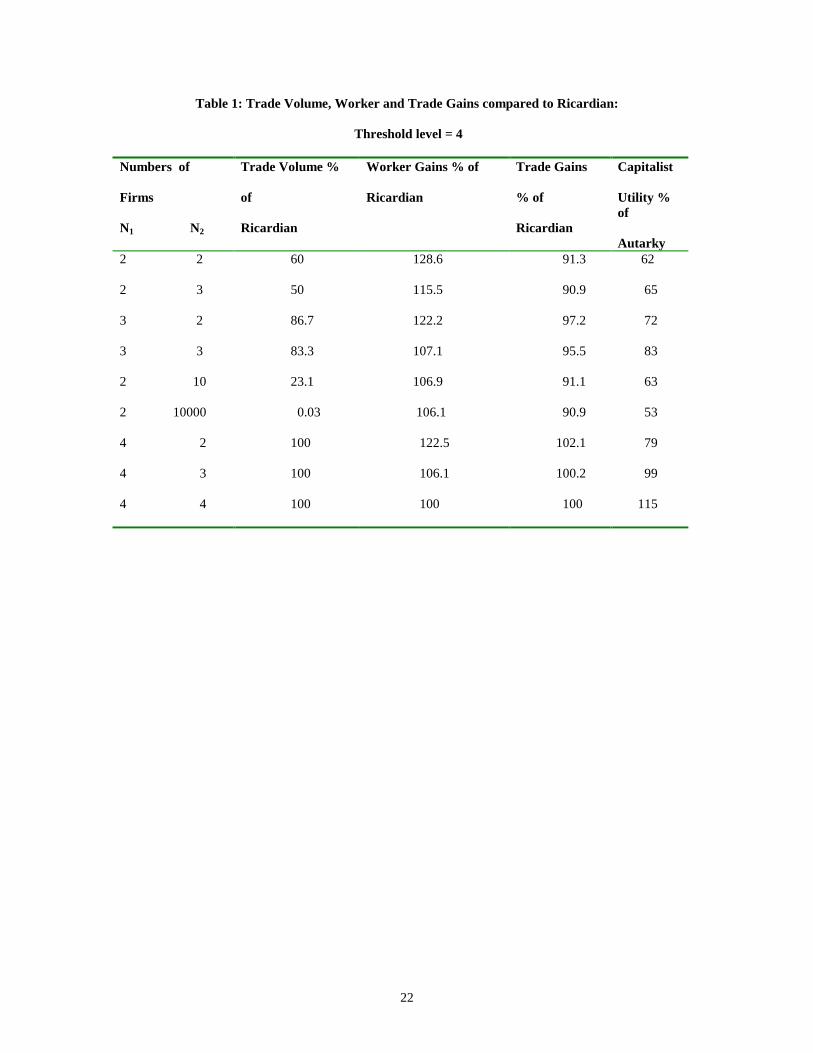
We begin with some numerical calculations to illustrate the propositions that follow. Table 1

shows the trade gains for workers and the economy as a whole compared to the Ricardian case for cases in

which the number of export firms does not exceed the threshold level. It also shows how the trade volume

changes as domestic competition intensifies. Inspection of the Table 1 shows that typically workers gain

more, and the economy less, than the competitive Ricardian case. All the columns are expressed as

percentage of the Ricardian value, except for the last column shown the utility of capitalists as a percent of

their autarky level(who earn nothing in the Ricardian model). This shows that the folk theorem appears to

apply more to workers than the economy at large. These results only make sense. When the numbers of

world export firms falls short of the threshold level the domestic import-competing industries are protected

by the oligopoly profits so that the gains from trade will be limited compared to the competitive case.

Workers, on the other hand, should gain more because world trade lowers industry profits. Capitalists lose

out from international trade because exporters now face the competition from foreign producers.

To calculate the gains from trade it is easiest to deal with the situation in which the numbers of

firms are the same in the pre-trade situation. In autarky, if N1 = N2 = N, we earlier showed that Y =

NL/(N-1) and Π = L/(N-1). To prove that workers gain more than in the competitive case, we need to

calculate the common price of each good under free trade when N = Nj (j = 1,2):

(26) p = N(a1 + a2)/(2N-1).

15

The utility of workers is always w/2(p1p2).5. Accordingly, in free trade, the utility of workers is simply

(since w = 1) 1/2p or (2N-1)/2N(a1+a2). In autarky, the wage is again 1 and the price of good i is pi =

aiN/(N-1); accordingly, worker utility is (N-1)/[2N(a1a2).5. The ratio of worker utility in free trade to that in

autarky is GW = [(2N-1)(a1a2).5/[(N-1)(a1 + a2)]. We learned earlier that in the gain from trade in the

competitive case is GR = (a2/a1).5. It therefore follows that ratio of worker utility in free trade to worker

utility in autarky is:

(27) Worker Gain = GW = [(2N-1)a1/(N-1)(a1+a2)]GR.

It follows that workers will gain more than the competitive case if and only if the coefficient of GR exceeds

unity. This will happen, clearing terms, if and only if (N-1)/N < a1/a2. But this is exactly the condition for

the number of firms to fall short of the threshold level! Thus:

Proposition 4. If the number of firms falls short of the threshold level and the number of firms is

the same across industries, workers gain more from free trade than they would in the competitive case. This

holds even though the gains from trade to the economy at large fall short of the competitive gains.

To see the intuition of the result, note that in the competitive case, before trade pi= ai. When trade

is opened, pi= a1 < a2 . Thus, free trade lowers the price of the natural import good but not the natural

export good. Since equal amounts are spent on each good, the gain from trade is roughly one-half of the

fall in the price of the natural import good. Thus, if a1=3 and a2= 4, the gain from trade would be roughly

16%. Now, in the oligopoly case, before trade is opened, pi = aiN/(N-1). When trade is opened, p =

N(a1+a2)/(2N-1). If N=2, before trade, p1 = 6 and p2 = 8. After trade, pi = 14/3 = 4.67, so the export

price falls by 22% and the import price falls by 41%. Clearly, the gain from trade for workers will be

larger. What happens is that in the competitive case, only the natural import industry faces more

competition. In the oligopoly case, both the export and import industries face more competition so prices

fall by a larger amount, benefiting workers more.

It is cumbersome to show analytically that capitalists lose out from free trade. Table 1 illustrated

the point with numerical calculations. However, the intuition is as follows. When N is less than the

threshold level, moving from autarky to free trade improves worker utility more than in the competitive

case, but since import-competing industries are protected by oligopoly profits, the economy as a whole

16

gains less than in free trade. The gain to workers is a cost to the capitalists. What happens is that

capitalists in every industry face more competition; and so their profits sink.

Post-Threshold Levels. We now turn to the quite different case of competition in the natural

export industries exceeding or equaling the threshold level. Here we will see that there is no presumption

that workers can gain more from trade than the competitive case, and trade actually helps oligopolists as a

whole. The threshold proposition almost immediately implies something about the gains from trade under

oligopoly compared to the competitive case. If the number of firms is equal across industries, Proposition

1 tells us that efficiency prevails in autarky. Proposition 3 tells us that when the number of export firms

exceeds or equals the threshold level, the free trade solution under oligopoly exactly reflects the Ricardian

trade solution. Thus, in this singular case in which in autarky firm numbers are the same across industries

and exceeds the threshold level, moving to free trade yields benefits to the economy that are exactly the

same as the Ricardian case. However, if the numbers of firms across industries in autarky are unequal, real

income will not be Pareto-efficient in autarky. In this important case, in which competition differs between

the two industries, the gains from trade must exceed the competitive case. Thus, by combining

Propositions 1 and 3 we can see:

Proposition 5. If the number of firms exceeds or equals the threshold level, then the gains from

trade exceed or equal the competitive case as the numbers of firms under autarky differ or are equal

across industries.

Now let us investigate the impact of trade on real wages separately from the gains from trade.

Going back to (13), we know the autarkic level of utility for workers. When competition in the export

industry exceeds or equals the threshold level, worker utility is simply Uworkers = (N1-1)L/2N1a1.

Comparing to (13), we see that workers will gain from trade if and only if

(28) [(N1-1)(N2-1)/N1N2a1a2].5 < (N1-1)/N1a1,

where N2 is now interpreted as the autarkic number of firms in the potential import-competing industry

(when trade opens, they vanish). Define the gain from trade for workers, Gw, as the ratio:

(29) Gw = [(N1-1)N2/(N2-1)N1].5GR ,.

where GR = (a2/a1).5, the gain from trade in the Ricardian case. Clearly, from (29), we get the following:

17

Proposition 6: If competition in the export industries exceeds or equals the threshold level,

workers gain more, the same, or less from free trade than the competitive case as autarkic competition in

the potential export industry (N1) exceeds, equals, or falls short of competition in the potential import-

competing industries (N2).

This result and Proposition 5 show that while the folk theorem appears to apply under the

specified circumstances to the gains from trade, it does not apply to workers. If there is more competition

in the import-competing industries than in the export industries of the two countries, free trade between

them will benefit workers less than if the reverse holds. This does not say that free trade hurts workers. It

simply says that if there is already a great deal of competition in the import-competing industries, their

gains will be limited compared to the situation in which there is more competition in the export industries.

In this post-threshold world, we will show now that free trade benefits capitalists as a whole. Of

course, the oligopoly profits of the natural import-competing industries vanish, but the natural export

industries face only a larger world market for their wares, since they face no new competition. They expand

their output and make greater profits. The gain in their profits exceeds the loss in the profits of the natural

import industries because the natural export industry is more profitable in autarky. To keep matters simple,

we stick to the case in which N1 = N2 = N. Autarky profits are easy to calculate. With our demand

assumption, the level of income is the same as Ricardo: Y = 2p1Q1 and Q1= L/2a1 since half of the labor

force will be in industry 1. But p1 = a1N/( N –1). Accordingly, Y = NL/(N –1). But wages are simply L

Subtracting, we obtain Π = L/(N - 1). The level of utility for capitalists is Π/2(p1p2).5; thus, using pi =

aiN/(N-1) we obtain:

(30) UAcapitalists = L/2N(a1a1).5.

Oligopoly profits in free trade are the same priced in labor units: Y = pL/a1 and p= Na1/(N-1); so again Y =

NL/(N-1). Subtracting wages L we again derive Π = L/(N-1). Thus, the level of utility is:

(31) UFTcapitalists = Π/2p = [L/2(N-1)][(N-1)/Na1] = L/2a1N.

Since a1 < (a1a2).5, it follows that capitalists gain from trade! Thus, combining previous results:

Proposition 7. If N1 = N2 = N, in the post-threshold level world, capitalists and workers gain

from trade.

18

This last proposition is extremely interesting for the contrast that it makes with standard trade

theory with two sources of income. We are accustomed to trade causing one group to suffer while another

gains. It is true that in this case the owners of licenses to produce the import-competing good lose out

from trade, but since no one is concerned with the distribution of income among capitalists it is still

interesting to point out that capitalists as a group and workers both gain from free trade in this special case

of my model.11

It is difficult to provide a general analysis of the gains to capitalists when the autarkic numbers of

firms are unequal. However, the intuition is simple and easy computer calculations show that if

competition in the export industry is not much higher than competition in the good in which each country

has a disadvantage, capitalists still gain from trade. However, if there is significantly more competition in

the export good (which lowers autarky profits) than among the producers of the other good (which raises

their autarky profits), the loss of profits in the import-competing industry from world trade will outweigh

the increase in profits in the export industry. In this case, capitalists as a group can lose from free trade.

This last proposition may be one of the most significant of the entire paper because it shows that

free trade should be expected to help stock market prices as well as real wages when competition around

the world exceeds the threshold level.

V. CONCLUSIONS

What have we learned? The folk theorem that under oligopoly free trade increases the gains from

trade through the pro-competitive effect is not true in general. It holds only in the circumstance that

opening the world to free trade leads to world efficiency. This will only happen if the world export

industries are sufficiently competitive. A key result is that there is a threshold level of the number of

Cournot oligopolists beyond which world efficiency reigns, but before which world economic inefficiency

prevails. In this latter case, oligopoly profits serve to prop up the domestic import-competing industries,

much like import tariffs would. Thus, it is easy to see that the gains from trade under oligopoly will not be

as great as with perfect competition unless the threshold level is reached.

The volume of international trade increases dramatically in the face of increases in competition.

This holds in particular when there is increased competition in the world export industries. To the extent

that world-wide movements in deregulation affects export industries more than import-competing

19

industries, we would expect that world trade would get quite a boost from this trend. However, if

deregulation favors the import-competing industries, quite the opposite conclusion holds. If deregulation is

economy-wide, we can expect large increases in world trade.

The real beneficiaries of international trade under oligopoly are the workers. The basic reason for

this is that free trade dramatically lowers commodity prices in terms of labor. The gains to workers will be

quite substantial when oligopoly profits are protecting natural import industries. International trade opens

these import-competing industries to competition, lowering their prices, and also increases the competition

facing the world's’export industries. Thus, profits, in this case, can fall dramatically and workers

experience a nice windfall from free trade because the increase in competition lowers all prices in terms of

labor. Perhaps this serves as a partial antidote to Stolper-Samuelson worries (Stolper and Samuelson,

1941). We find that when comparative advantages are sufficiently large or oligopolies sufficiently weak,

so that oligopoly profits do not protect the natural import industries, then both workers and capitalists as a

whole gain from international trade. The intuition is simply that workers gain because the prices of imports

fall and capitalists gain because natural export industries gain the world market (and their profits likely

exceed the losses of the natural import industries). With weak oligopolies, protectionism would be

expected to lower stock market valuations.

The main results of the paper, however, do not depend on our simplifying assumptions; for the key

to the model is that as firm numbers increase, high-cost firms eventually exit… the existence of which is the

hallmark of Ricardian comparative advantage. Indeed, since it is a basic characteristic of nearly any kind

of oligopoly that prices fall with competition, the intuition of the model does not depend on any of its

special features (unit elastic market demand; Cournot behavior). The simplifying assumptions merely

enable us to derive the conclusions in a simple way without having to overcome self-imposed obstacles.

An important extension of the model would be to show how robust the results are to dropping the

symmetry assumption. This would entail assuming that the utility functions might differ between

countries. I think it would be easy to reverse the result that with domestic competition more than the

threshold levels, the opening of free trade will raise overall profits, just by assuming that the natural export

industries are relatively unimportant in the grand scheme of things, which cannot happen under symmetry.

20

However, the key is whether there is a plausible empirical presumption that overall profits rise on the move

to free trade.

Another extension would be to add more countries. This would increase the threshold level of

competition in any one country, because the smaller the country the less likely it can drive foreign

competitors out of business. However, it would seem to then matter quite significantly whether a subset of

countries moves to free trade or the world.

21

REFERENCES

Brander, J. A. 1981. Intra-industry trade in identical commodities. Journal of International Economics 11:1-14.

Brander, J. A. and P. Krugman. 1983. A reciprocal dumping model of international trade. Journal ofInternational Economics 15:313-321.

Chang, W. W. and S. Katayama. 1995. Trade and policy of trade with imperfect competition. In W. W.Chang and S. Katayama, eds. Imperfect Competition in International Trade. London: Kluwer AcademicPublishers.

Chipman, J. S. 1965. A survey of the theory of international trade: part I, the classical theory.Econometrica 33: 477-519.

Cordella, T. and J. Gabszewicz. 1997. Comparative advantage under oligopoly. Journal of InternationalEconomics 43:333-346.

Dixit, A. K. and J. E. Stiglitz. 1977. Monopolistic competition and optimum product diversity. AmericanEconomic Review 67: 297-308.

Fisher, E. 1988. Market structure in a Ricardian model of international trade. Mimeo.

Helpman, E. and P. Krugman. 1986. Foreign Trade and Market Structure. Cambridge: MIT Press.

Kemp, M. C. and M. Okawa, 1995. The international diffusion of the fruits of technical progress underimperfect competition. In W. W. Chang and S. Katayama, eds. . Imperfect Competition in InternationalTrade. London: Kluwer Academic Publishers.

Krugman, P. R. 1979. Increasing returns, monopolistic competition and international trade. Journal ofInternational Economics 9: 469-479.

Lerner, A. P. 1943. The concept of monopoly and the measurement of monopoly power. The Review ofEconomic Studies 11: 157-175.

Markusen, J. R. 1981. Trade and gains from trade with imperfect competition. Journal of InternationalEconomics 11:531-551.

Mueller, D. 1986. Profits in the Long Run. Cambridge: Cambridge University Press.

Ruffin, R. J. 1971. Cournot oligopoly and competitive behavior. Review of Economic Studies 38: 493-502.

Ruffin, R. J. 1988. The Missing Link: The Ricardian approach to the factor endowment theory of trade.American Economic Review 78:759-772.

Ruffin, R. J. 1991. Cournot oligopoly and Bertrand competition. Mimeo. The University of Houston.

Stolper, W. and P. Samuelson. 1941. Protection and real wages. Review of Economic Studies 9: 58-73.

Venables, A. J. 1985. Trade and trade policy with imperfect competition. Journal of InternationalEconomics 19: 1-19.

Wilcox, C. 1950. On the alleged ubiquity of oligopoly. American Economic Review 49: 67-73.

22

Table 1: Trade Volume, Worker and Trade Gains compared to Ricardian:

Threshold level = 4

Numbers of

Firms

N1 N2

Trade Volume %

of

Ricardian

Worker Gains % of

Ricardian

Trade Gains

% of

Ricardian

Capitalist

Utility %of

Autarky2 2 60 128.6 91.3 62

2 3 50 115.5 90.9 65

3 2 86.7 122.2 97.2 72

3 3 83.3 107.1 95.5 83

2 10 23.1 106.9 91.1 63

2 10000 0.03 106.1 90.9 53

4 2 100 122.5 102.1 79

4 3 100 106.1 100.2 99

4 4 100 100 100 115

23

FOOTNOTES

1 M.D. Anderson Professor of Economics, the University of Houston, Houston, TX, 77204, and ResearchAssociate, Federal Reserve Bank of Dallas. Thanks are extended to Nick Feltovich, Ron Jones, JeffreyCampbell, Peter Mieszkowski, Roger Sherman, and Joel Sailors for their comments. I have benefited fromcomments at seminars at the Universities of Rochester and the Houston. All errors are due the author andthe Federal Reserve System is not responsible for the views expressed.2 Clair Wilcox is seldom acknowledged in the trade literature, but should be. He was not only a industrialorganization expert, he was also deeply interested in international trade. Indeed, it was he who drafted andpresented the famous 1930 petition of 1028 economists to President Hoover that signing the Smoot-Hawley tariff bill would “injure the great majority of our citizens” with detailed references to the effects onspecific industries. See the New York Times, May 5,1930.3 I paraphrase here a similar comment in Wilcox (1950) on the classic A & P case.4 For a recent summary see Chang and Katayama (1995).5 Ruffin (1971) shows that for the case of unitary price elasticity that the usual conditions for stability aresatisfied for oligopoly. More details are in Ruffin (1991).6 See Ruffin (1988) for the use of the Mill-Graham utility function in the Ricardian model; and for theclassic earlier treatment see Chipman (1965).7 The reader in a hurry may skip Proposition 2; for the actual paper uses a later and simpler propositionbased on a symmetrical model.8 It is interesting to note that the threshold levels would be smaller in the presence of fixed costs. I amindebted to Jeffrey Campbell for this observation.9 In the non-symmetry case, we would have to add the equation Q1 + Q1* = (Y + Y*)/2p. But this isimplicit in the above equations.10 This is a point made by Markusen (1981).11 It should be noted that this proposition does not depend on the assumption that in each country half of allincome is spent on each good. As long as we assume symmetry, half of world income will be spent oneach good so that the natural export industries will still earn the same profit as in the case underconsideration.