old-age support and demographic transition in developing ... · 2 old-age support and demographic...
TRANSCRIPT

UCD GEARY INSTITUTE
DISCUSSION PAPER SERIES
Old-age support and demographic transition in
developing countries. A cultural transmission
model
Javier Olivera
UCD Geary Institute,
University College Dublin
Geary WP2013/07
7 May, 2013
UCD Geary Institute Discussion Papers often represent preliminary work and are circulated to encourage
discussion. Citation of such a paper should account for its provisional character. A revised version may be
available directly from the author.
Any opinions expressed here are those of the author(s) and not those of UCD Geary Institute. Research
published in this series may include views on policy, but the institute itself takes no institutional policy
positions.

2
Old-age Support and Demographic Transition in
Developing Countries. A Cultural Transmission
Model
Javier Olivera
UCD Geary Institute,
University College Dublin
This version, 07-May-2013
Abstract: We model intergenerational old-age support within the context of a developing country that faces demographic transition: declining fertility and increasing life expectancy. We attempt to answer if agents will be able to support their parents during the next generations and under what conditions. For this purpose we use a three period overlapping generations model and a cultural transmission process, in which agents may be socialized to different cultural family models (old-age supporters and non-supporters). As life expectancy increases, we find conditions under which a reduced fertility rate is compatible with the expectation to be supported during old-age. This offers an additional explanation for the persistency of family old-age support in developing countries facing demographic transsition.
JEL classification: J13; D10; E24 Keywords: Cultural transmission; intergenerational transfers; fertility Correspondence to: Javier Olivera, UCD Geary Institute, room b108, University College Dublin, Dublin 4, Ireland (e-mail: [email protected] / [email protected]). Acknowledgements: I appreciate the comments and suggestions by Erik Schokkaert, Thomas Baudin, Philip O’Connell, and my doctoral committee. The usual disclaimers apply.

3
1. Introduction
Perhaps the most familiar stylised facts of the demographic transition are the continued fall
of the fertility rate and infant mortality and the increase of life expectancy, which reduce
population growth and increase the proportion of the elderly. Although at different paces,
almost all societies experience the demographic transition. This is well advanced and close
to complete in developed countries and emerging in developing countries.
According to the theory of intergenerational wealth flows (Caldwell, 2005) or the old-
age security approach (Nugent, 1985), the fall of fertility in developing countries is a result
of the decline of the old-age insurance value of children. In contrast, for the economic theory
of the family (Becker and Barro, 1988; Willis, 1973, 1982), the driver of fertility decline is the
change in available economic opportunities (e.g. high rearing costs, more female labour
participation; more education). Some economists have also acknowledged the importance of
culture and changing preferences for the determination of fertility (see Pollack and Watkins,
1993), and cross-cultural psychologists have provided useful empirical support. For
instance, Kagitcibasi (1982; 2007) and Trommsdorff (2009)1 argue that the economic value of
children has declined (and will continue decreasing) in favour of a more prominent role for
an emotional or psychological value of children, which will lead to the reduction of fertility
as well as a change in how children and old-age care are valued in society. This perspective
is interesting because it takes account of culture as an important driver of the evolution of
fertility and old-age support. Furthermore, Fernandez and Fogli (2006) show
econometrically that both culture (measured by the fertility rate of the country of ancestry)
and personal experience matters for fertility decisions. Although culture is also
acknowledged in Blackburn and Cipriani (2005) as an important factor to explain the decline
of fertility, this is not explored. Instead, the authors give a leading role to intergenerational
transfers to explain the demographic transition. Their model shows two distinctive
equilibria: societies that combine high levels of development, low fertility with strong
downstream intergenerational transfers versus societies with low development, high fertility
and strong upstream intergenerational transfers. In this paper, we consider whether tensions
between different cultural values towards old-age support within a society play a role in the
determination of the fertility rate.
1 This thesis is built on the basis of the results of the Value of Children study implemented during the 70’s and replicated during the 2000’s in a pool of societies that differ in culture and degree of modernization.

4
If we accept that parents have children to insure against old-age related risks, the
continued decrease of fertility rates and increase of life expectancy imply that children must
support their old parents longer and with the help of fewer siblings, which increase the cost
of this support. In developed countries social security institutions help to overcome this
burden; but in developing countries these institutions are scarce, the family being the main
mean for insuring against old-age. Therefore, the demographic transition poses a challenge
for these countries. Given that family old-age insurance is widely available in developing
countries, what is the rationale behind the long run demographic projections that show
parents living longer and having fewer children? One may think of a more intensive use of
social security as a way to cope with this challenge, but this might not be the case. For
instance, some Latin American countries launched pension systems in order to alleviate old-
age related risks, but there is still a considerable proportion of families that do not
participate in such schemes2. How can we reconcile the decision of individuals of having
fewer children and expecting family old-age support within societies where more
institutionalised forms of old-age support are scarce and longevity is increasing?
The goal of this paper is twofold. First, in order to examine whether culture matters to
decisions about fertility and old-age support in developing countries, we build a framework
where socialization to certain cultural values plays a central role in old-age support and
fertility. This model can analyse the demographic transition in developing countries in the
presence of important norms of family old-age support. Second, we examine the
consequences of the demographic transition for the ability of households to adequately
insure their older members. For these aims, we propose an Overlapping Generations (OLG)
model of three periods with a cultural transmission process à la Bisin and Verdier (2001). In
this process parents transmit their preferences or traits to their children, who must choose
one of those traits under the influence of vertical (parental) and oblique (societal) cultural
socialization. This transmission is made via a costly socialization effort. We consider that
parents inculcate some cultural values related to the importance of old-age support (e.g.
filial piety) to their children with the goal of obtaining economic support during old-age. We
denote this cultural trait “old-age supporters”. At the same time, children are exposed to
2 These countries favoured pension systems based on individual capital accounts in a major reform wave during the 90’s, but the number of enrolled and contributors in the pension system have decreased instead of increase (Arenas de Mesa and Mesa-Lago, 2006). Hence, the family still plays the most important role for old-age protection. Furthermore, those countries will experience a significant drop of the TFR and increase of the life expectancy. Between 1955 and 2050, the TFR will drop from 5.89 to 1.85, and the life expectancy at birth will rise from 59.8 to 79.6 (database of the Economic Commission for Latin American and the Caribbean).
5
other cultural values that could imply a different response to old-age care. For example,
users of social security or any other forms of saving for old age may emphasize the cultural
value of being independent, i.e. neither supporting old-age parents nor being supported by
own children. This trait is called “non old-age supporters”. That fact that there are only two
cultural traits is clearly a simplification of reality, but is enough to reflect the tension
between different perspectives on the value of children. This tension is acknowledged in
Kagitcibasi (1982, 2007) when the author describes the evolution of the value of children as a
result of the development and urbanization process.
There are other applications of the cultural transmission model (see the survey of Bisin
and Verdier, 2010). Baudin (2010) uses a cultural transmission framework to study the
population dynamics of a society where two cultural types with different fertility norms
(modernists and traditionalists) compete. The work of Bisin and Verdier (2001) also
discusses the population dynamics of different cultural transmission technologies. To our
knowledge, the study of intergenerational transfers has not yet been studied within this
framework. There are some works dealing with intergenerational transfers within
endogenous fertility growth models, but the culture component is missing. For instance,
Raut and Srinivasan (1994), Chakrabarti (1999) and Morand (1999) show how societies arrive
at different equilibria of fertility, growth and human capital when intergenerational
transfers are considered. In an OLG model, Palivos (2001) shows how different family–size
norms lead to multiple equilibria, but intergenerational transfers are not considered. We
contribute to the literature by studying intergenerational support in developing countries
with an OLG model where fertility, socialization effort and the distribution of cultural types
are endogenous. In addition, the results of the model are stressed by considering exogenous
improvements in longevity.
One of the major results of this paper is to account for the demographic transition by
showing how the increase of longevity may reduce fertility and the expected old-age
transfer from children. The mechanism is that the old-age supporter type receives an
expected transfer amount from her children that is influenced by the direct socialization of
the parent (in her own image) and the proportion of types in society. The socialization effort
affects directly the probability of embracing the parental type, so that the parent must
increase their cultural socialization effort to extract enough old-age transfers from her
children. As socialization effort is costly, fewer resources are devoted to childbearing and
hence the fertility of this type drops. The non old-age supporter types react by increasing
their socialization effort because they want to offset the influence of the other type in the

6
cultural transmission to their own children. Therefore, they reallocate resources from
childrearing to socialization, and this pushes down their fertility. Overall, fertility of both
types declines and socialization effort increases. While we analyse the long run equilibria,
we conjecture that a continued increase of longevity and the cultural response of the old-age
supporter can jeopardise the existence of this trait. This is a well cast example of non
efficient cultural reaction to the economic environment. Moreover, we inspect the effects of
implementing a compulsory pension scheme and a more tolerant setting between the types
on our conjecture. We find that these “solutions” help to improve the ability of children to
support parents and avoid or delay the extinction of the old-age supporter trait.
The rest of the paper is organized as follows. The model is set out in section 2. Section 3
deals with the effects of the demographic transition and section 4 shows two extensions of
the model. Finally, section 5 concludes.
2. The model
We consider an OLG model with three periods: childhood, adulthood and old age. During
childhood, individuals are socialized towards certain cultural models by their parents
(vertical socialization) and society (oblique socialization) following a cultural transmission
process à la Bisin and Verdier (2001). Individuals are inculcated family cultural values on the
commitment of giving old-age support to parents. We restrict the set of cultural types to
two: 1) old-age supporters and 2) non old-age-supporters. A type 1 person supports
financially her old parents and expects to be supported by her children in old-age as well. A
type 2 person does not support her parents, saves for her own consumption in old-age, and
does not expect to be supported by her children.
represents the fraction of individuals with cultural type 1 and is the fraction of
individuals with type 2. Subscript t indicates time. Children are born without any cultural
trait and are first exposed to the parent’s cultural type. Socialization to parental cultural type
i occurs with probability , i{1,2}. If the socialization of the child towards her parent’s
cultural type i fails (which occurs with probability ), she picks another cultural type
randomly from the adult population, which means that type 1 is chosen with probability
and type 2 with probability . The probability that the child of a parent with cultural
type i is socialized to cultural type j is
. The transition probabilities for i,j{1,2} are:
and
(1)

7
and
(2)
The success of vertical socialization depends on the effort of the parent to socialize
her child to her own cultural type, i.e.
. This effort costs . Depending on how
the cultural transmission technology is specified, vertical and oblique cultural transmission
may be substitutes or complements. In the first case, the parent belonging to the major type
has less incentives to socialize her children to her cultural type because she can free-ride
from her dominant position in society3. If more parents in society have type i, the probability
of having a child with the same type i is larger; however, the less dominant types will
increase their vertical socialization effort in order to not disappear. In the second case,
parents from the minority type socialize their children to the major type. An example of this
is cultural assimilation. The conditions and set up of the cultural transmission model will
lead to the specific socialization technology.
The parent is able to know the consequences of the possible socio-economic actions of
her children but she evaluates those actions through her own preferences. It is assumed that
the parents always prefer to have children with the same cultural type. In this sense, the
parent acts myopically or paternalistically towards her children. We denote
as the increase in the utility of a type i parent who has a child with type j. After
normalization, we assume:
Assumption 1: for , with , and
(3)
Having a child with the same cultural type is the best state for a parent , but a
child embracing another type is the least tolerated state ( ) whatever the type of
the parent. The difference measures the intolerance of an individual with
cultural type i towards type j; therefore in our matrix, both cultural types disfavour the other
types symmetrically (Bisin et al, 2009). However, it is arguable that a type 2 parent may be
more tolerant to cultural deviation than a type 1 parent. We study this possibility in a
further section.
3 Bisin and Verdier (2001) refer to this as the cultural substitution property, which is needed to reach a distributional equilibrium with heterogeneous types.

8
Assumption 2: a)
; b)
.
We assume that the probability of success of vertical socialization equals the
socialization effort made by the parent. Although not evident here, we will show later that
socialization effort is an endogenous response from parents that depends on as well. The
cost of one unit of socialization effort is c, which is expressed as time cost and is common to
all cultural types.
Once the individual has embraced a cultural type at the end of childhood, she has to
decide her consumption level, fertility and socialization effort in her adulthood. This
individual is endowed with one unit of time which she must allocate to labour, childrearing,
old-age financial support for her parents (or savings) and effort to socialize her children
towards her own cultural type. Type 1 individuals decide their socialization effort, fertility
and consumption respecting the following budget constraints:
(4)
(5)
The adult receives wage per unit of time worked. We do not distinguish wage by
cultural type and take it as given (similar to Chakrabarti, 1999 and Palivos, 2001). It is also
considered that preferences on consumption are defined above subsistence levels of
consumption in adulthood (v) and old-age (m). Adult consumption is financed with the
wage net of the time cost of rearing children, the time cost of socialization effort and the
fraction transferred to the old parent. This last term corresponds to the share of a total
old-age transfer that each child should transfer if all siblings were type 1, i.e.
. As considered by some OLG growth models with old-age support (e.g. Raut
and Srinivasan, 1994; Chakrabarti, 1999 and Morand, 1999), the old-age financial support is
an exogenous fraction of the labour time. Children who adopt type 1 values do not transfer
money on top of the share resulting from equal division among siblings; which means that
parents are not financially compensated for possible cultural deviation. We can think of B as
a result of a social norm under which children must support (equally) old parents with a
transfer. Given that cultural deviation is possible, the value of B is just a reference and it is
assumed that it is well above subsistence level. For the same reason, consumption in old-age

9
is an expected value4. For now, we assume that minimum consumption constraints are
not binding, but later on we relax this assumption.
Type 2 adults choose their socialization effort, fertility, consumption and savings
according to the following budget constraints:
(6)
(7)
Type 2 does not support financially her parent; instead, she saves a fraction during
adulthood and consumes all her savings (times the interest factor R1) during old-age. In
case of cultural deviation, we rule out the possibility that type 1 children donate a transfer to
a type 2 parent. As specified before, bt is only intended for parents who are type 1. To give
support to this assumption, we may invoke a sort of demonstration effect within three
generations such as argued in Cox and Stark (2005). This effect is observed when a parent
supplies support to her own parent to instil the same behaviour from her children. Thus, we
may consider that a type 1 child will not support her type 2 parent as this last one did not
support her own parent. In addition to the budget constraints, it is necessary to add some
time and non negativity constraints:
(8)
(9)
(10)
All adults maximize the following utility function. We use a logarithmic function for
tractability reasons.
(11)
As in other OLG models (Raut and Srinivasan, 1994; Morand, 1999; Palivos, 2001) the
only productive stage is adulthood and the individuals do not consume during childhood,
there are no bequests and both parents (mother and father) are only one entity. A type i
4 Note that type 1 adults use probabilities of period t to construct the expected transfer corresponding
to t+1, due to their inability of predicting future probabilities. Furthermore, given that ,
equation 5 can be reduced to .

10
derives utility from her consumption during adulthood and old-age. The parameter is a
time discount factor. The number of children also generates satisfaction to adults through
the parameter . Endogenous fertility models as in Becker and Barro (1988) and Dahan and
Tsiddon (1998) also include the number of children as a source of utility for the parent. The
last term in equation 11 represents the gains in utility that an adult expects from the cultural
transmission process; as mentioned before, a parent prefers a child with the same cultural
type. Moreover, the restrictions on the parameters are and one has to assume5
in order to get a positive number of children at any . Finally, the dynamics of
the model is governed by:
(12)
Equation 12 shows the dynamics of distribution of types through the proportion of
cultural type 1 in period t+1. If the total population in period t is , then are type 1
and are type 2. The number of type 1 individuals at t+1 is formed by i) the
children of type 1 parents who becomes type 1:
; ii) the children of type 2 parents
who become type 1:
and iii) the type 1 parents who become old parents:
. If we divide the sum of all these individuals over the total population at t+1:
and cancel the term , we obtain equation 12.
2.1 Behaviour of cultural type 1
Under assumptions 1-2, equations 1-2 and provided that subsistence consumption levels are
not binding, each adult finds the optimal values of her consumption, fertility and
socialization effort
by maximizing equation 11 subject to equations 4 and 5.
As is the share of time dedicated to childbearing and the social norm transfer
cannot be dishonoured by type 1 individuals, the maximum number of children is limited to
.
(13)
(14)
5 Furthermore, this assumption leads us to get the expected signs for partial derivatives (
and ).

11
where
>
. For a given period t, figure 1 shows the
possible interior solutions of and
as a function of the distribution of types in the same
period.
FIGURE 1: FERTILITY AND SOCIALIZATION EFFORT FOR TYPE 1
0 1
1
0 1
Note that when not constrained,
and
. The kink in the socialization effort
comes from the non negativity constraint on . The probability of having a child with
cultural type 1 rises with the share of this type in the adult population, therefore the
individual chooses a higher fertility rate in order to increase the gains in utility of having a
child with the same cultural type. The result
is the cultural substitution property
invoked in Bisin and Verdier (2001). This means that a type 1 individual expends less time in
socialization and relies more on the oblique socialization by the society to socialize her
children. In this way, the majority group invest less in socialization. Under this property, the
authors prove that an equilibrium with a heterogeneous distribution of types is possible.
The minimum number of children is
. It is interesting to note that fertility
depends negatively on the old-age transfer, i.e. if the parent lives longer and thus needs
more money in old-age, then fertility declines. We explore this in more detail in section 3.
The maximum value that optimal socialization effort may reach is
or unity.
2.2 Behaviour of cultural type 2
Similar to type 1, type 2 finds the optimal values of her consumption, fertility and
socialization effort
by maximizing equation 11 subject to equations 6 and

12
7. As before, the highest rate of fertility is bounded by the share of time dedicated to
childbearing and the savings needed to consume in old-age:
.
(15)
(16)
(17)
where
<
. To ease comparisons, figure 2 shows the possible
interior solutions, for a given period t, of and
as a function of type 1’s distribution.
FIGURE 2: FERTILITY AND SOCIALIZATION EFFORT FOR TYPE 2
0 1
1
0 1
We observe
and
because of the same reasons explained for type 1; the
latter derivative confirms that vertical and oblique cultural transmissions are substitutes.
The number of children is between
and
. Socialization effort is zero when
due to the non negativity constraint on and it cannot be larger than
or unity.
The savings rate depends on the altruism and discount parameters rather than on the
interest factor due to the logarithmic form of utility and the fact that constraints are not
binding. This result is similar to that of De la Croix and Doepke (2003).
2.3 Dynamics
The dynamics of the distribution of types is governed by . After some
algebra applied on equation 12, we can arrive to the expression
. It is

13
easily observable that {0;1} are equilibria of the system as well as all which solve
. The stability of these equilibria is not easy to assess given that the system of
equation 12 is non-linear of second order and has kinks. However, it is possible to find that
{0;1} are unstable, while the other equilibria arise from chaotic dynamics, so that it is hard to
study their stability. Nonetheless, we can show that the system has an analytical solution
until critical value c=c*; once this threshold is passed (i.e. when c < c*), the system undergoes
a bifurcation and then presents chaotic dynamics6. Figure 3 shows the optimal dynamic
paths for each value of c (at step of 0.0025) considered in the computation of the path7.
FIGURE 3: POPULATION DYNAMICS
Starting from the right we observe that there is only one steady state (hyperbolic fixed
point in bifurcation theory), which decreases with the reduction of c; and then, the
bifurcation occurs around c=0.0897. After this threshold, the system undergoes a period-
doubling bifurcation and then a chaotic dynamics. Interestingly, the system reaches another
set of hyperbolic fixed points at . The threshold c* comes from , i.e
. Thus, if (or equivalently ), the system undergoes a bifurcation and
then chaos.
6 Given that it is possible to find real life or standard values used in literature for all parameters, but c, we choose this parameter to evaluate the dynamics of the model. 7 For figure 3, we use =0.154; =0.3433; =0.99; q0=0.95. The same chaotic shape is found with the use of other parameter values and initial conditions. Further, in section 3.3 we will argue about the values of these parameters.
0.2
0.3
0.4
0.5
0.6
0.7
0.8
0.9
1.0
0.010 0.023 0.035 0.048 0.060 0.073 0.085 0.098 0.110 0.123 0.135
% o
f ty
pe
1 (
q)
cost of socialization effort
14
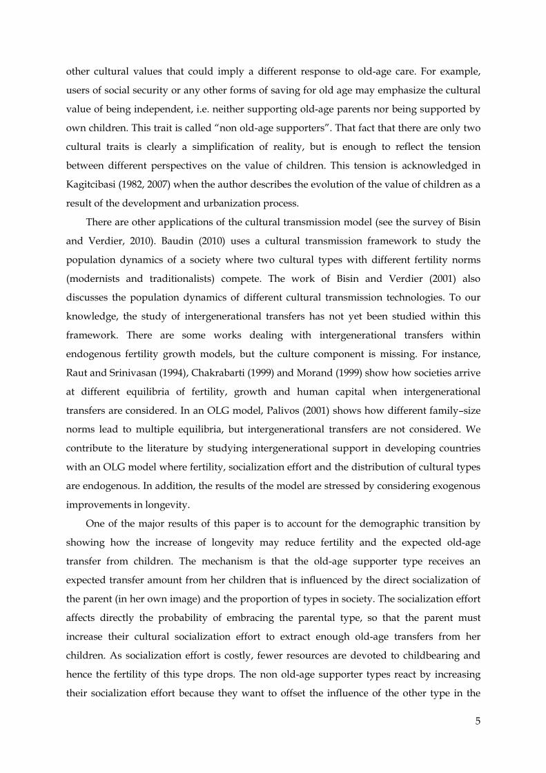
Proposition 1: For initial conditions
, with no binding consumption
constraints and assumptions 1-2,
are equilibria of
the dynamic system 1-17. {0;1} are unstable, and is stable if . The stability of is
only locally guaranteed if because the dynamic system undergoes a bifurcation
when
.
Proof: see appendix.
The point means that the system can reach an heterogeneous distribution of types,
which is stable if . In order to ease the interpretation of the dynamics hereafter, we will
assume the following restrictions on the parameters: . It is straightforward to obtain
as and
are equal to zero for and , respectively. Under these
dynamics the socialization effort of both types is zero at equilibrium8, which is obviously a
particular case of the more general Proposition 1 (which allows for non-zero values of
socialization efforts at steady states). However, this is sufficient to easily describe how types
interplay with each other given their optimal responses on fertility and socialization. Recall that
for values there are multiple equilibria with not assured stability, so that we would not
be able to draw regular relations between types. Figure 4 represents the dynamics when
.
FIGURE 4: DYNAMICS OF THE DISTRIBUTION OF TYPES
0 1
0 1
The initial conditions for the distributions of types (q0) might be placed at any point in
[0,1]. In the interval adults do not make any socialization effort and fertility is
determined without any influence of the distribution of types. It means that the initial
distribution of types satisfies every individual. The most interesting cases arrive when
8 This dynamics may be observed in societies where socialization effort is expensive.

15
or . In the first case, the proportion of type 1 is low in society, so that
type 1’s children have a high probability of embracing type 2; this, in turn, reduces the
expected value of the old-age support. If individuals with type 1 want to be supported
enough during old-age by their children, they have two means: socialize more intensively
their children towards their own type and having more children. As a result, the proportion
of type 1 increases (left panel of figure 4). Given the substitutability between vertical and
oblique socialization, declines over time and stops at (right panel of figure 1). The
other reaction of type 1 is to increase fertility over time up to (right panel of figure 4).
Thus, at point individuals with type 1 reach a desirable distribution of types.
If , type 2’s children have a high probability of embracing the other cultural
type. Given that a type 2 adult prefers a child with her own cultural type, she increases her
socialization effort and fertility in order to obtain a desirable distribution of types such that
she can derive enough utility from the cultural alignment between her and her child. In this
process, the share of type 2 increases as observed in the left panel of figure 4. Socialization
effort decreases and fertility increases over time (figure 2 and right panel of figure 4,
respectively) up to , with and being the final values of socialization and
fertility.
3 Demographic transition
3.1 Living longer
As mentioned in the introduction, the continued increase of longevity is well-documented in
many and different populations. This phenomenon may affect decisions on fertility and
other relevant variables, and importantly, it might challenge the financial support from
children to old parents in populations where old-age family insurance is prominent. We can
use our theoretical framework to highlight the possible consequences of higher longevity,
which we treat as exogenous9.
A way to easily introduce the rise of life expectancy in the model is to assume that an
increase of life expectancy is equivalent to an increase of the minimum old-age
consumption, m. We therefore consider the case that constraint 5 is binding. We also assume
9 Although, there are models dealing with the endogenization of life expectancy (for instance Ponthiere (2010) relates longevity as an outcome of lifestyle and Leroux et al (2011) include genetic and behavioural factors to explain differences in longevities), we treat this variable as exogenous to avoid unnecessary complexity in the model.

16
that adulthood consumption constraint is not binding. Indeed, we will keep this assumption
through the rest of this chapter given that we focus on the effects of the increase of life
expectancy and such constraint does not change our model’s main implications. As the
inclusion of a binding old-age constraint produces optimal responses that depend on wage
levels, we assume no growth of wages ( ) in order to simplify the analysis,
otherwise we should add human capital accumulation which is beyond the focus of our
model. Equations 18 and 19 show the optimal fertility and socialization effort when m binds
for type 1:
(18)
(19)
where
>
.
Results of equation 18 and 19 are possible only if
; otherwise the constraint
cannot be satisfied10. Different from the previous program, fertility and socialization effort
are affected by wages and minimum old-age consumption level m. As evident from
equations 18 and 19, a rise of life expectancy in period t reduces fertility and increases
socialization effort. An increase of m triggers a positive variation of socialization effort from
parents in order to raise their chances to receive enough transfers to fulfil minimum old-age
consumption, which implies that there are fewer resources to invest in childbearing and
hence fertility falls. From the re-arranged equation 5,
, it is
clear that a parent must increase her socialization effort to cope with a rise of life expectancy
in period t. Certainly, an increase of her fertility in period t could only improve the expected
value of old-age consumption for the next generation of parents and not for her. The reason
is that a rise of in t would increase the proportion of type 1 in t+1 (
from equation
12) and hence the corresponding transition probability that affects the expected transfer
amount ( . Therefore, the adult in period t does not find it useful to increase her fertility
10
Equation 19 may be rearranged as
, which should be greater than unity if
.
Thus, is truncated to 1. Replacing this value into equation 5 leads to
, i.e. the transfers from children might be insufficient to cover minimum old-age consumption.

17
to meet the value of m in old-age. Indeed, she reduces her fertility to free resources and
reallocate them to socialization effort.
The old-age transfer B is considered fixed and exogenous, arising from a social norm
related to support for elderly parents. However, it is plausible that a rise of life expectancy
may eventually push up this value. Comparative statistics of a change in the transfer B
might illustrate the effects on fertility and socialization. As expected,
from equation
19, i.e. parents need to socialize their children less intensively due to the higher transfer B.
The effect of the transfer B on fertility is less clear and depends on the position of and on
the value of B when m begins to bind. Proposition 2 states these effects for type 1:
Proposition 2: a) if m binds at any , then i)
if and ii)
if
; with threshold
. b) if m binds at any , then
.
Proof: see appendix.
A rise of the old-age transfer will increase fertility only if the original value of B is small
enough (less than threshold z). As we pointed out before, a higher value of B reduces
which in turn reduces utility (last term of equation 11). However, this cultural loss might be
compensated by the adult with an increase of her fertility. Of course, the increase of B and
fertility also pushes down utility through the reduction of the first period consumption as
the adult must raise the transfer given to her own parent and pay for more children. But
these extra expenses can be financed with the resources freed up from socialization effort. In
the case that B is large, the burden of paying the old-age transfer is already heavy, so that an
increase of fertility would only deteriorate first period consumption without compensating
the cultural loss. Therefore, reducing fertility is the best response from the adult when B is
already large enough.
If old-age consumption constraints are binding for type 2 ( ), the
optimal responses are:
(20)
(21)
(22)

18
As in the program without binding constraints,
and
. This time fertility is
positively affected by the interest factor and by wages due to income effects. A rise of R (or
w) lowers the savings rate needed to reach minimum old-age consumption and frees
resources that may be invested in childbearing. Different from the program without binding
constraints, the savings rate is determined by the interest factor in order to get exactly m
during old-age. A rise of m in period t reduces fertility because the adult must meet the
higher value of m by devoting more resources to savings and less to childrearing.
Furthermore, the rise of m does not affect socialization effort in period t, which is explained
by the fact that type 2 adults do not need to socialize their children to their cultural type to
reach the old-age consumption m11. They socialize children solely for cultural reasons.
3.2 Distribution of types
As we are interested in the evolution of old-age support in developing countries, we will
focus on societies with initial conditions . These societies are mainly populated by
type 1 individuals, the economic value of children is high and the social norm of supporting
parents is extended. However, these characteristics and values will start to change at some
point of the society’s development which may lead to the formation of other values
incompatible with old-age family support. This evolution is a consequence of (and
reinforced by) forces such as urbanization, social security, modernization. We hypothesise
that cultural transmission models are valid mechanisms for such change of values12.
If , the final equilibrium distribution of types ends at
. It is
straightforward to observe how a change of the value of parameters may alter this
equilibrium13. This would be the final equilibrium if life expectancy -that is equivalent to
minimum old-age consumption- did not play a role. The top panel of Figure 5 plots the old-
age consumption level of type 1 for each distribution. Given that
if
and if , the consumption path is decreasing when comes from
. Recall that the cultural process is starting from , therefore the relevant area of
analysis in figure 5 is from to the left. We observe that if the value of m is low, this
never binds old-age consumption, so that will be the final distribution.
11 For this reason, and are equal to the values found in the system without binding constraints. 12 Others could be diffusion (e.g. through media), change of social norms like family size norms, etc. 13 For instance, a continued increase of childrearing costs, as is commonly acknowledged across countries, leads to a continued reduction of the share of type 1. Furthermore, the old-age support becomes more difficult to afford for future generations.
19
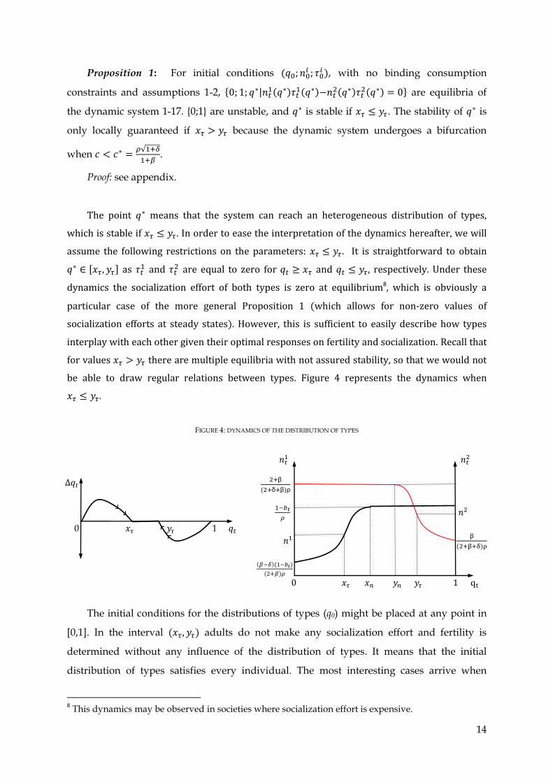
FIGURE 5: DISTRIBUTION OF TYPES AND INCREASE OF LIFE EXPECTANCY
m’ m 0 1
0 1
0 1
The final equilibrium of the system ( ) will be different if m binds. We may consider
that the minimum old-age consumption has been increasing over time due to the rise of life
expectancy so that the line m moves up like in figure 5´s top panel14. To determine the
location of this equilibrium, we must observe the middle panel. There, if the old-age
consumption is not binding, the dotted and thin curves represent and
, respectively. At
the point where the old-age consumption is binding ( ), the socialization effort curve
that is relevant for type 1 is not any more the dotted one, but the one from equation 19
represented by the bold line. Now, type 1 will cease his socialization effort only if there is a
distribution of types at least as large as , which will allow her to reach the minimum old-
age consumption. Therefore, if 15, then the equilibrium will be within the interval
14 In order to ease the explanation and construction of figure 5, we assume that type 2’s old-age consumption is not binding. Proposition 3 will consider fully the binding constraints for both types. 15 In parameter values, this means
.

20
as depicted in figure 5’s middle panel. If , then the distribution of types will
be as the system started from .
Now, equilibrium implies a positive amount of for type 2, but this is
compensated by having fewer children. As figure 5’s third panel depicts, type 2’s fertility is
computed at instead of , which entails a lower fertility. Furthermore, type 1 must
allocate more resources to socialization in equilibrium than in equilibrium , although
this is compensated by a reduction of fertility. This drop of fertility can also be observed in
the third panel of figure 5: the relevant fertility curve for type 1 is now the bold curve (which
represents equation 18) instead of the dotted one. At the new equilibrium , type 1 fertility
is lower. All these results are formalized by the next proposition.
Proposition 3: For a society with and , a rise of life expectancy -expressed
as an increase of minimum old-age consumption- leads to a distribution of types or
if and , respectively. Furthermore distribution implies that
socialization effort of both types is positive at equilibrium, and fertility declines overall.
Proof: see appendix.
Moreover, as a result of the previous proposition (provided that ), the larger is m
the larger is the share of type 1 in the distribution. This happens because equilibrium is
within the interval and a rise of m also increase the value of , which in turn,
enlarges the interval to the right. Thus, the society strengthens the values related to old-age
family insurance as a reaction to the increase of life expectancy.
3.3 An illustration
The next example illustrates the dynamics of fertility and socialization. The parameter
values are set in table 1 and the results are depicted in figure 6.
TABLE 1: PARAMETER VALUES
c R B m w
0.99 0.3433 0.154 0.154 2.9126 0.35 0.30 1.0
Initial values:
0.95 6.1 0.0 2.07 0.88
There is a wide range of assumed values for in the literature of OLG models. For
example this value is 0.075 in De la Croix and Doepke (2003) and the authors imply that a
21
family could have up to 27 children. However, that number could not be reached because of
biological limits. Bongaarts (1982) points out that, theoretically, the maximum number of
children (births per woman) should be between 13 and 17. Accordingly, these limits are 6.5
and 8.5 children per person. We consider that 6.5 children per person is enough as an upper
limit, so that we assume =0.15416. We also assume that the cost of socialization effort is not
different from the cost of rearing17. The discount factor value is assumed for convenience:
under this value, type 2’s old-age consumption is equal to m. Note that the implied yearly
discount rate of is 4.37% if the adulthood period lasts 25 years, which is within other
values assumed in OLG simulations (2% in Lau, 2009 and 4.7% in De la Croix and Doepke,
2003). For consistency, we assume this interest rate to compute the interest factor. As we set
m=0.30, the reference transfer B is located above it at level 0.35. For all these parameters, the
unconstrained consumption devoted to old-age period lies between 0.33 and 0.23, so that the
minimum old-age consumption constraint will bind at some point.
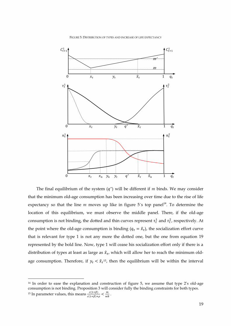
FIGURE 6: PATHS TOWARDS EQUILIBRIUM
16 According to the information from the Demographic and Health Surveys Program (http://www.measuredhs.com), the simple mean of the percentage of mothers with 10 or more children is only 1.65% for a pool of 13 Latin American countries. 17
As rearing costs, activities related to socialization effort are also costly. Examples of these are the time spent with children, the search of a neighbourhood to reside in which the family finds more cultural homogeneity, and of the school to which the child is sent (Bisin and Verdier, 2001).
0.50
0.55
0.60
0.65
0.70
0.75
0.80
0.85
0.90
0.95
1.00
1 3 5 7 9 11 13 15 17 19 21 23 25 27
qt
t
no binding constraint
m binds
1.5
2.5
3.5
4.5
5.5
6.5
1 3 5 7 9 11 13 15 17 19 21 23 25 27t
n1,n2
n2|m binds
n1
n2
n1|m binds

22
Figure 6 accords with the explanations stated in the previous section. If life expectancy
does not play a role, the distribution of types would be =0.666 (see bold line of figure 6’s
top left panel) and the fertility rates of type 1 and 2 would be 6.12 and 3.88, respectively,
which results in a weighted fertility rate of 5.37. However, in our simulation m binds from
period 4, so that the final equilibrium is reached at =0.762 and fertility of both types ends
at lower levels (figure 6’s top right panel). The overall fertility rate decreases to 2.71.
Furthermore, from the point m starts to bind, type 1 increases her socialization (figure 6’s
bottom panel). Once the equilibrium is reached, both types end with positive values of
socialization effort. In Table 2 we show the sensitivity of the final equilibrium with respect to
changes in the parameter values.
TABLE 2: FINAL EQUILIBRIA FOR DIFFERENT PARAMETER VALUES
Parameter values
Overall
n
baseline 0.762 2.69 2.80 2.71 0.40 0.38
0.175 0.736 2.29 2.48 2.34 0.46 0.42
0.200 0.702 1.95 2.20 2.03 0.52 0.46
c 0.175 0.782 2.71 2.82 2.73 0.34 0.33
0.200 0.800 2.75 2.86 2.77 0.29 0.28
0.800 0.734 2.44 2.61 2.49 0.46 0.43
0.700 0.715 2.32 2.51 2.37 0.50 0.46
For instance, it is intuitive that an increase of means that having children is more
expensive relatively to socializing them, so that the fertility rate drops and the socialization
effort rises. The opposite occurs when socialization cost increases. Furthermore, q* drops
when rises as type 1 has fewer children and must devote more resources to socialization
effort in order to meet consumption m in old-age. Type 2 also increases socialization effort
but relatively less than type 1 because they do not need to exert a transfer from their
0.0
0.1
0.2
0.3
0.4
0.5
0.6
0.7
0.8
0.9
1.0
1 3 5 7 9 11 13 15 17 19 21 23 25 27t
1,2
2
1|m binds
1

23
children. This prevents fertility rate of type 2 to fall more than type 1’s; and at the end, the
proportion of type 1 drops. If adults are less altruistic, they will have fewer children, so that
socialization effort may increase.
Finally, table 3 highlights the consequences of an increase in life expectancy on the final
equilibrium q*. As mentioned in the previous section, a continued increase of life expectancy
–measured through m- leads to a decline of overall fertility and a strengthening of type 1’s
values by a larger socialization effort. Type 2 also increases her socialization effort in order
to face the increasing proportion of type 1 in society.
TABLE 3: FINAL EQUILIBRIA FOR DIFFERENT VALUES OF m
m Overall
n
0.300 0.762 2.69 2.80 2.71 0.40 0.38 0.305 0.772 2.60 2.73 2.63 0.44 0.42
0.310 0.782 2.52 2.66 2.55 0.48 0.45 0.315 0.793 2.44 2.59 2.47 0.52 0.49
0.320 0.805 2.36 2.53 2.39 0.56 0.52
0.325 0.818 2.27 2.46 2.31 0.61 0.56
As mentioned before, transfers from children would be insufficient to cover parent’s
minimum old-age consumption if m continues increasing such that
. We might
conjecture that if the old-age transfer does not increase, then old-age consumption falls short
of subsistence level, which would lead to an increase of chronic poverty among the elderly.
Alternatively, if the individual can only finance a fraction
years of the total potential
increase in life expectancy, this effect may also be interpreted as the inability of type 1 to
take advantage from the exogenous increase in longevity. This suggests that there will be
differentials in life expectancy once the individuals reach old-age, i.e. type 2 will live longer
than type 1. Therefore, the position of type 2 in the distribution of types may become
stronger in society through their higher proportion of elderly people, which reinforces the
fall of the expected value of the old-age transfer. The continued fall of type 1’s fertility (and
reduction in the number of siblings) makes unbearable the payment of the old-age transfer,
so that type 1 could eventually disappear. The same result is obtained even when the social
norm of supporting elderly parents is strong enough to push for a rise of B in order to meet
minimum old-age consumption. A rise of B allows the parent to fulfil minimum old-age
consumption but also implies fewer resources for childbearing, which in turn reduces type
1’s fertility. As B continues increasing to finance the increase of m, type 1’s fertility falls
considerably, even at the point where childbearing is not profitable. These conditions also

24
would jeopardize the existence of type 1. The next section shows some extensions to the
model, which might moderate or delay the effects of the mentioned conjectures.
4. Extensions
In this section we still consider a society with characteristics and and analyse
how our previous results change when i) the assumption of symmetric tolerance levels is
relaxed and ii) a social security scheme is introduced.
4.1 Relaxing the assumption on the intolerance levels
Assumption 1 might be relaxed by allowing different levels of tolerance between types. We
keep the normalization =1 for i{1,2} and set . The higher (with ij), the
more tolerant is each type towards the other. The program is easily solved for type 2
irrespective of whether the old-age consumption constraint is binding or not, but it is
algebraically tedious for type 1 when the old-age consumption constraint is not binding. If
this constraint binds for type 1, then does not play a role any more as type 1’s
socialization effort is entirely determined by the pursuit of meeting minimum consumption
in old-age (see equation 19). As we intend to illustrate the sensitivity of our previous results,
it is enough to consider values and to simulate the final equilibria (see table
4). This implies that type 2 is more tolerant to cultural deviation than type 1, which seems a
reasonable assumption.
TABLE 4: FINAL EQUILIBRIA AND TOLERANCE LEVELS ( )
Overall
n
0.00 0.762 2.69 2.80 2.71 0.40 0.38 0.05 0.785 2.84 2.93 2.86 0.34 0.33
0.10 0.807 3.04 3.09 3.05 0.26 0.25
0.15 0.829 3.31 3.32 3.31 0.17 0.17 0.20 0.848 3.70 3.66 3.69 0.06 0.06
One of the clear results is that parents socialize children less intensively towards their
own type because cultural deviation is more tolerated. If type 2 parents are more tolerant,
then they reduce their socialization effort, and consequently q* increases. As q* rises, type 1
parents need less investment in socialization effort. Therefore, socialization effort drops
overall, which frees resources to invest in childbearing so that fertility rises overall as well.
Although not shown in the table, a more tolerant environment, i.e. with a higher , delays

25
the time at which the old-age consumption constraint starts to bind. For example, in the
simulation of section 3.3 that considers , m=0.30 begins to bind in period t=4. If the
tolerance level is or , the same value of m starts to bind at period t=6
and t=10, respectively. And for values , m=0.30 will never bind. In sum, in a
more tolerant society agents invest less in socialization effort and more in childbearing, and
therefore the period at which children fail to be an adequate old-insurance is delayed.
4.2 Introduction of compulsory social security contribution
Developing countries where old-age family transfers are prominent may also have a pension
system scheme. The characteristics are diverse: it can be PAYG, fully funded, based on
individual accounts, compulsory, voluntary, etc. Therefore, it is interesting to assess the
effects of a compulsory contribution to pensions on fertility, socialization and dynamics of
our model. We will assume that a pension scheme based on individual capitalization is
enforced in the model. This type of scheme is, for example, the most common in the Latin
American countries. The pension contribution -a share of wages - is paid during
adulthood by all individuals and the returns R are received during old-age, which is easily
introduced into the system equations.
Old-age consumption is not binding
It is algebraically tedious to find the analytical solutions for type 1 when the old-age
consumption constraint is not binding. However, the computation of type 1’s first order
conditions with different values of allows us to conclude that fertility falls with the
contribution rate18. As our interest is focused on societies with (recall that =0), the
contribution rate will not affect socialization effort of type 1 when the old-age consumption
restriction is not binding. Equations 23 and 24 describe the optimal responses for type 2:
(23)
(24)
18
The introduction of the social security contribution decreases fertility through two channels: there is an income effect due to less disposable resources for childbearing, and a substitution effect between
R and , which reduces the need of having children to fulfil elderly consumption.

26
The contribution rate will not affect directly type 2’s fertility and socialization effort if
. As the model is set (the voluntary old-age savings is equivalent to ), an
increase of in period t will perfectly substitute the same quantity of personal old-age
savings, and hence it should not have any effect on the outcome variables in period t.
However, when we simulate the optimal path of type 2’s socialization effort and fertility, we
observe that a rise of reduces socialization effort and increases fertility in the following
periods. The reason is that –as mentioned- the increase of lowers type 1’ fertility, which
reduces type 1’ share in the total population. Therefore, type 2 devotes less time in
socialization, which in turn frees resources to be allocated to fertility. If , the voluntary
savings rate becomes zero, being the total amount of savings; i.e. the individual is
forced to save more than she would like. In this case, clearly an increase of reduces type
2’s fertility. The final effect of a change of in period t on socialization in t+1 is
undetermined.
Old-age consumption is binding
Equations 25 to 28 show the optimal fertility and socialization effort when old-age
consumption restriction binds:
(25)
(26)
where
and
.
(27)
(28)
In general, standard models of fertility and growth predict that the increase of social
security may lower fertility (Becker and Barro, 1988; Boldrin and Jones, 2002). For instance,
Barro and Becker (1988) treat the increase of social security contributions and benefits as an
increase of the cost of rearing a child, so that fertility should drop –at least temporarily- due
27
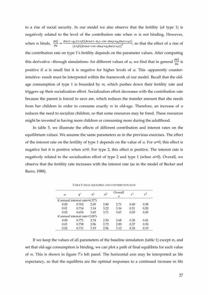
to a rise of social security. In our model we also observe that the fertility (of type 1) is
negatively related to the level of the contribution rate when m is not binding. However,
when m binds,
, so that the effect of a rise of
the contribution rate on type 1’s fertility depends on the parameter values. After computing
this derivative –through simulations- for different values of , we find that in general
is
positive if is small but it is negative for higher levels of . This -apparently counter-
intuitive- result must be interpreted within the framework of our model. Recall that the old-
age consumption of type 1 is bounded by m, which pushes down their fertility rate and
triggers up their socialization effort. Socialization effort decreases with the contribution rate
because the parent is forced to save , which reduces the transfer amount that she needs
from her children in order to consume exactly m in old-age. Therefore, an increase of
reduces the need to socialize children, so that some resources may be freed. These resources
might be invested in having more children or consuming more during the adulthood.
In table 5, we illustrate the effects of different contribution and interest rates on the
equilibrium values. We assume the same parameters as in the previous exercises. The effect
of the interest rate on the fertility of type 1 depends on the value of . For =0, this effect is
negative but it is positive when >0. For type 2, this effect is positive. The interest rate is
negatively related to the socialization effort of type 2 and type 1 (when >0). Overall, we
observe that the fertility rate increases with the interest rate (as in the model of Becker and
Barro, 1988).
TABLE 5: FINAL EQUILIBRIA AND CONTRIBUTION RATE
Overall
n
if annual interest rate=4.37% 0.00 0.762 2.69 2.80 2.71 0.40 0.38
0.01 0.714 3.14 3.22 3.16 0.21 0.20
0.02 0.676 3.65 3.71 3.67 0.05 0.05 if annual interest rate=2.00%
0.00 0.771 2.74 2.50 2.68 0.38 0.41 0.01 0.738 2.96 2.72 2.89 0.27 0.30
0.02 0.711 3.19 2.96 3.12 0.18 0.19
If we keep the values of all parameters of the baseline simulation (table 1) except m, and
set that old-age consumption is binding, we can plot a path of final equilibria for each value
of m. This is shown in figure 7’s left panel. The horizontal axis may be interpreted as life
expectancy, so that the equilibria are the optimal responses to a continued increase in life

28
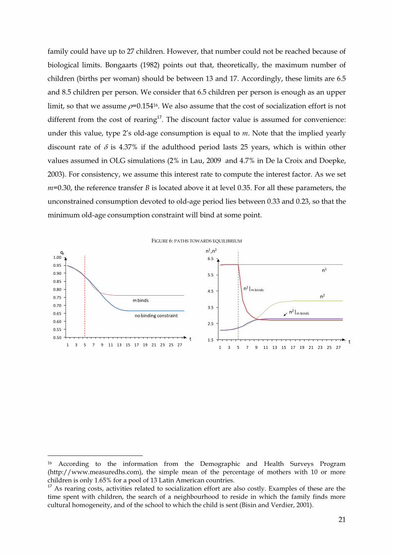
expectancy. If there is no social security (=0.0 and old-age transfer remains constant,
B=0.35), then type 1 is unable to take advantage from the exogenous increase of life
expectancy once the point m=0.35 is reached (indicated by the peak in figure 7). From that
point, type 1 can only finance a fraction
years of the total potential increase in life
expectancy (as conjectured in section 3.3); meanwhile, her fertility continues falling as is
observed in the right panel of figure 7. At that point and later, type 2 can reallocate more
resources from socialization to childrearing and increases fertility as q* is falling. The
reduction of the share of type 1 in the distribution is reinforced by the rise of type 2’s fertility
and the fact that the expected old-age transfers go down (which triggers up)19. Eventually,
the number of type 1’s children may be too low to cope with the burden of old-age support
to parents, so that at some point type 1 could stop having children and disappear, provided
that B or other variables remain unchanged. However, the introduction of social security
might mitigate this effect as can be observed in figure 7. For instance, a contribution rate of
0.02 may delay the declining of the type 1’s share in the distribution up to the point where
m=0.408 (see the peaks of the dotted lines in figure 7). Furthermore, if there is no social
security, reproduction of type 1 may stop at m=0.4168 (q*=0.76). But, if =0.02, type 1
extinguishes at 0.4675 (q*=0.711).
FIGURE 7: FINAL EQUILIBRIA FOR DIFFERENT LEVELS OF m
4.3 Trends and demographic projections in Latin American countries
Demographic trends in Latin American countries indicate a substantial fall of fertility and
increase of life expectancy. Given that these economies show a prominent role for old-age
19 Although not shown in figure 7, the overall fertility declines.
0.50
0.55
0.60
0.65
0.70
0.75
0.80
0.85
0.90
0.95
1.00
0.30
0.31
0.32
0.34
0.35
0.36
0.37
0.38
0.40
0.41
0.42
0.43
0.44
0.46
=0.02=0.00
q*
m
0.50
1.00
1.50
2.00
2.50
3.00
3.50
4.00
0.30
0.31
0.32
0.34
0.35
0.36
0.37
0.38
0.40
0.41
0.42
0.43
0.44
0.46
n1|=0
n2|=0
n1|=0.02
n1,n2
m
n2|=0.02

29
family transfers, one could think that the structural pension reform undertaken during the
90’s might help the population to cope with the old-age risk, but this is not really true as the
rates of coverage are low (38.7% of employed). These rates are as low as 13.0% in Peru at the
national level (2.6% in rural areas) or as high as 65.3% in Costa Rica. Furthermore, poverty
rates are particularly high in rural areas; there, type 1 values are more important and hence
the budget of the families is very likely to be bounded by subsistence consumption20.
The introduction and strengthening of compulsory social security theoretically
enhances old-age consumption and help for the sustainability of type 1 in the long run, but it
is observed that in practice only salaried workers from the formal sector contribute to
pensions. The informal sector may be huge and diverse, ranging from 30.7% of the labour
force in Chile to 64.6% in Peru; 49.2% being the simple average. An easy way to observe how
the informal sector size reduces the effectiveness of social security is by adding , the
probability of belonging to the informal sector, into the consumption constraints of the
model21:
and
and
Now, the consumption is a weighted sum of the consumption obtained in the formal
sector (paying ) and in the informal sector (=0). Clearly, a larger informal sector is
equivalent to a lower contribution rate.
As pointed, the decline of fertility and rise of life expectancy threatens the ability of type
1 to afford minimum old-age consumption, and even their existence in the long run. The
Governments of Latin American countries cannot rely on the support of children to parents
as a permanent way to face the ageing of population. Hence, it is understandable that a
pension system is launched as a way to help agents to obtain a certain level of consumption
in old-age. However, informality might reduce the scope of this system through a lower
expected contribution rate. Although our model does not distinguish individuals according
to their occupation in the formal or informal sector, salaries or other socio-economics
characteristics, it is possible to incorporate them and evaluate more precisely the relations
20 All these figures come from the database of the Economic Commission for Latin American and the Caribbean. 21
This may be interpreted as once the individual embraces a type, she is randomly assigned to the
informal sector with probability . Of course, probability distributions of types and informality are not necessarily independent, but assuming the contrary would add unnecessary complexity.

30
found within the framework of a country with a high share of informality. Note that
workers earn lower salaries in the informal sector, so that minimum consumption will bind
their budgets more easily than that of formal workers. An additional option is a change of
the cultural tolerance levels of society, although this is hardly applicable from a policy
intervention point of view.
5. Conclusions
Cultural models of family matter for the dynamics of fertility. The addition of a cultural
transmission technology means that our model can better account for the demographic
transition. This shows how the increased life expectancy may reduce fertility and expected
old-age transfers through the strengthening of cultural socialization efforts. While we
analyse the long run equilibrium, we suggest that a continued increase in life expectancy
may weaken inclinations to provide old-age support for older generations. This is a good
example of non-efficient cultural reaction to the economic environment. Furthermore, we
have shown that societies becoming more tolerant or the introduction of compulsory social
security might improve the ability of children to support parents and counteract the
weakening of old-age support. Finally, in an application, our model may highlight some of
the future demographic pressures and the possible deterioration of the standard of living of
the elderly in Latin American countries.

31
References
Arenas de Mesa, A. and C. Mesa-Lago (2006), “The Structural Pension Reform in Chile:
Effects, Comparisons with other Latin American Reforms, and Lessons”, Oxford Review
of Economic Policy, 22(1): 149-167.
Baudin, Thomas (2010), “A Role for Cultural Transmission in Fertility Transitions”,
Macroeconomic Dynamics, 14(4): 454-481.
Becker, G. S., and R. J. Barro (1988), “A Reformulation of the Economic Theory of Fertility”,
Quarterly Journal of Economics, 103: 1–25.
Bisin, A. and T. Verdier (2001), “The Economics of Cultural Transmission and the Dynamic
of Preferences”, Journal of Economic Theory, 97: 298-319.
Bisin, A. and T. Verdier (2010), “The Economics of Cultural Transmission and Socialization”,
NBER Working Paper No. 16512.
Bisin, A., G. Topa and T. Verdier (2009), “Cultural transmission, socialization and the
population dynamics of multiple-trait distributions”, International Journal of Economic
Theory, 5: 139–154.
Blackburn, K. and G.P. Cipriani (2005), “Intergenerational transfers and demographic
transition”, Journal of Development Economics 78: 191-214.
Boldrin, M. and L. E. Jones (2002), “Mortality, Fertility and Saving in Malthusian Economy”,
Review of Economic Dynamics 5: 775-814.
Bongaarts, J. (1982), “The Fertility-Inhibiting Effects of the Intermediate Fertility Variables”,
Studies in Family Planning, 13(6/7): 179-189.
Caldwell, J. (2005), “On Net Intergenerational Wealth Flows: An Update”, Population and
Development Review, 31(4): 721-740
Chakrabarti, R. (1999), “Endogenous Fertility and Growth in a Model with Old Age
Support”, Economic Theory, 13(2): 393-416.
Cox, D. and O. Stark (2005), “On the demand for grandchildren: tied transfers and the
demonstration effect”, Journal of Public Economics 89: 1665-1697.
Dahan, M. and D. Tsiddon (1998), “Demographic Transition, Income Distribution, and
Economic Growth”, Journal of Economic Growth, 3: 29–52.
De la Croix, D. And M. Doepke (2003), “Inequality and Growth: Why Differential Fertility
Matters?”, The American Economic Review, 93(4): 1091-1113.
32
Fernandez R. and A. Fogli (2006), “Fertility: The Role of Culture and Family Experience”,
Journal of the European Economic Association April-May 2006 4(2–3): 552–561.
Kagitcibasi, Cigdem (2007), “Family, Self, and Human Development Across Cultures:
Theory and Applications”, Second Edition.
Kagitcibasi, C. (1982), “Old-age security value of children: Cross-national socioeconomic
evidence,” Journal of Cross-Cultural Psychology, 13: 29-42.
Lau, S.-H. Paul (2009), “Demographic structure and capital accumulation: A quantitative
assessment”, Journal of Economic Dynamics & Control 33: 554–567.
Leroux, M.L., P. Pestieau and G. Ponthiere (2011), “Longevity, Genes and Efforts: An
Optimal Taxation Approach to Prevention“, Journal of Health Economics 30(1): 62-76.
Morand, O. (1999), “Endogenous Fertility, Income Distribution, and Growth”, Journal of
Economic Growth, 4: 331–349.
Nugent, J. B. (1985), “The Old-Age Security Motive for Fertility”, Population and
Development Review 11: 75–97.
Palivos, T. (2001), “Social Norms, Fertility and Economic Development”, Journal of
Economic Dynamics and Control, 25: 1919-1934.
Pollack, R. and S. Watkins (1993), “Cultural and Economic Approaches to Fertility: Proper
Marriage or Mesalliance?”, Population and Development Review, 19(3): 467-496.
Ponthiere, G. (2010), “Unequal Longevities and Lifestyles Transmission”, Journal of Public
Economic Theory, 2010, 12 (1), pp. 93-126.
Raut, L.K. and Srinivasan, T.N. (1994), “Dynamics of endogenous growth” Economic
Theory, 4: 777-790.
Trommsdorff, G. (2009), “A social change and human development perspective on the value
of children”, in: Perspectives on Human Development, Family, and Culture, S. Bekman
and A. Aksu-Koç (eds.). Cambridge: Cambridge University. Press, pp. 86-107.
Willis, R. (1973), “A new approach to the economic theory of fertility behavior”, Journal of
Political Economy, Supplement (March/April): S14-S64.
Willis, R. (1982), “The Direction of Intergenerational Transfers and Demographic Transition:
The Caldwell Hypothesis Reexamined”, Population and Development Review, 8: 207-
234, Supplement: Income Distribution and the Family.

33
Appendix
Proof of proposition 1:
The dynamic is governed by
. In this system, the steady
state q* is locally stable is
. First we check equilibriums 0 and 1:
For equilibrium q*=0, we have and
. Thus,
(A1)
where
;
;
and
.
As
, the equilibrium q*=0 is unstable.
For equilibrium q*=1, we have and
. Thus,
(A2)
where
;
and
.
, so that the equilibrium q*=1 is unstable.
Now, we distinguish two cases of different parameter values:
a) :
If initial condition is , then and
, and hence the dynamics stops at
equilibrium . Similarly, if initial condition is , then ,
and the
equilibrium is . If is initially located within the range ( , then there is no
motion in the system and hence remains at .
a.1) If :
If is initially located within the range ( , then there is no motion in the system and
hence remains at . For any small disturbance , the system
does not go back to q* because there is no motion within and hence q* is unstable.
a.2) If :
We evaluate equation A1 at q*= :

34
a.3) If :
We evaluate equation A2 at q*= :
a.4) If
As , a small disturbance in the boundary of q* may lead to positive socialization
effort, thus we construct with and
. Furthermore,
and
:
(A3)
And
, so that q* is stable.
b) :
The steady state q* is obtained from solving in equation A3, i.e.:
. We evaluate stability of q* by taking the derivative of equation A3:
(A4)
where
and
.
If , then and ; and hence W<0. The sign of X is undetermined.
However, the expression multiplying X in A4 should be zero as this is the condition to find
equilibrium q*. Furthermore, the expression multiplying W in A4 is positive due to
. Therefore,
and q* is stable.
For this q* we have inspected -with simulations- that the system undergoes a bifurcation
near
. When c passes this threshold (i.e. c<c*), the system initially undergoes a
period-doubling bifurcation, and then it becomes chaotic and hard to analyze (like in figure
3). This chaotic behaviour is produced by the dynamics summarized in equation 12, which is
a non-linear second order difference equation (and with kinks). Therefore, we can only state
that q* is locally stable.

35
Proof of proposition 2:
a) Provided that , we can find the distribution of types at which the old-age
consumption binds:
; and this is
. We
replace into equation 18 (recall that and ) and obtain optimal fertility
. The sign of
is not conclusive as
. If we define threshold z=
, then
if ; and
if .
b) Provided that , then , so that
. Therefore,
and
.
Proof of proposition 3:
a) Distribution when :
We know that m binds type 1´s consumption at ; m can also bind type 2´s
consumption or not. If m binds type 2’s consumption, then the steady state is
obtained from (
) provided that and . Similarly, is
also the steady state when m does not bind type 2’s consumption (solving
).
b) Distribution when :
We proof that when by contradiction. We know that m binds type 1´s
consumption at . Assume that m does not bind type 2´s consumption. If ,
; and if
,
. But, given that we are assuming ,
these values are a contradiction as and
are zero only at and ,
respectively. Therefore,
and consequently . The same results apply if m
also binds type 2´s consumption.
When m binds, the fertility differential for type 2 is
.
This expression is negative if
, which holds given that
is equivalent to
. The type 1´s fertility differential is
when m
binds (at
). This expression is negative if
, which holds given that
36
this is equivalent to . Recall we are evaluating steady states and that
must be lower than as we assume dynamics with and .
Therefore, fertility falls overall when equilibrium is . From that point, it is
clear that and
depend negatively on m.