oil price changes and the oslo stock exchange
TRANSCRIPT

Oil Price Changes and the Oslo Stock Exchange
A study of how oil price changes affected the Oslo Stock Exchange between 1990-2009
Department of Statistics Authors:
Bachelor Thesis Autumn 2011 Sheida Ghadakchian
Supervisor: Peter Gustafsson Arild Pettersen

1
Abstract
This paper addresses how oil price changes affect the Oslo Stock Exchange. Multiple
linear regressions with eight explanatory variables have been used to investigate the
relationship between oil and the Oslo Stock Exchange between 1990-2009. The time
period has also been divided into two sub periods to investigate if the effects of oil
price changes have become more prominent over the years. After deliberating
between univariate and multivariate models we decided to use a multiple linear
regression. The six sources of error of the OLS model have been thoroughly discussed
and examined. The variables used in the regressions have been selected by revising
previous research and economic theory.
The results for the entire period show that oil had a significant positive effect on the
stock market with a coefficient of 0.24. This was not unexpected and is in accordance
with our hypothesis. The same result was obtained for the first sub-period, 1990-1999.
However, looking at the second sub period, 2000-2009, oil proved not to be
significant. This result was surprising as it is contradictory to most previous research.
Despite not being significant, investigations of the relationship between oil prices and
the stock market showed that they remained rather correlated. This profound result is
very interesting and might be explained by an underlying variable our model has not
been able to capture.
Keywords: Oil price, Oslo Stock Exchange, Multiple Linear Regression, Mean
Average Process

2
Table of Contents
1. Introduction ............................................................................................................. 4
1.1 Purpose and research question ........................................................................................ 4
1.2 Limitations and data ........................................................................................................ 4
1.3 Methodology ................................................................................................................... 5
1.4 Disposition ...................................................................................................................... 5
2. Revised Literature .................................................................................................. 6
3. The Oil Sector and Stock Exchange ....................................................................... 9
3.1 Pricing of oil .................................................................................................................... 9
3.2 Oil price development ................................................................................................... 11
3.3 Pricing of a stock ........................................................................................................... 11
3.4 Oslo Stock Exchange .................................................................................................... 12
3.4.1 Sector Composition ............................................................................................... 14
4. Regression parameters ......................................................................................... 15
4.1 Dependent variable ....................................................................................................... 15
4.2 Explanatory variables .................................................................................................... 16
4.2.1 Gross Domestic Product ........................................................................................ 16
4.2.2 Interest rate ............................................................................................................ 16
4.2.3 Inflation.................................................................................................................. 17
4.2.4 Oil .......................................................................................................................... 17
4.2.5 FTSE 100 and S&P 500 ......................................................................................... 17
4.2.6 Exchange rate NOK/USD and NOK/GBP ............................................................. 18
5. Modeling ................................................................................................................. 19 5.1 Multiple linear regression ............................................................................................. 19
5.2 Ordinary Least Square................................................................................................... 20
5.3 Sources of error ............................................................................................................. 21
5.3.1 Homoscedasticity ................................................................................................... 21
5.3.2 Autocorrelation ...................................................................................................... 22
5.3.3 Normal distribution ................................................................................................ 24
5.3.5 Stationarity ............................................................................................................. 27
6. Results and analysis .............................................................................................. 28
6.1 Original regression ........................................................................................................ 28
6.1.1 Sub-period 1: 1990-1999 ....................................................................................... 31
6.1.2 Sub-period 2: 2000-2009 ....................................................................................... 32
6.1.3 Moving Average Process ....................................................................................... 33
7. Conclusion .............................................................................................................. 35
8. References .............................................................................................................. 37
Appendix ..................................................................................................................... 41

3
Equations
Equation 1 Pricing of stocks
Equation 2 Regression model
Equation 3 Gross Domestic Product
Equation 4 Multiple Linear Regression
Equation 5 OLS condition 1
Equation 6 OLS condition 2
Equation 7 OLS condition 3
Equation 8 OLS condition 4
Equation 9 OLS condition 6
Equation 10 Multiple Linear Regression
Equation 11 Whites test: Residuals
Equation 12 Whites test: Variance
Equation 13 Durbin Watson test
Equation 14 Jarque Bera test
Equation 15 Subsidiary equations
Equation 16 VIF
Figures
Figure 1 Oil value chain
Figure 2 Oil supply and demand curve
Figure 3 Oil price development
Figure 4 Oslo Stock Exchange development
Figure 5 Sector composition
Figure 6 Residuals vs time
Figure 7 Normality test
Figure 8 Oil price and stock prices
Figure 9 Moving avarage process
Tables
Table 1 Correlation matrix between stock exchanges
Table 2 Whites heteroscedasticity test
Table 3 Durbin Watsons autocorrelation test
Table 4 VIF-values
Table 5 Regression 1990-2009
Table 6 Significant variables in regression 1990-2009
Table 7 Regression 1990-1999
Table 8 Regression 2000-2009

4
1.
Introduction
Norway’s oil and gas journey started in the late 1950s when the Dutch found gas in
the Norwegian Sea. On the 13th
of April 1965, 22 exploration and production licenses
were rewarded to different contractors and already during the summer of 1966 the
first well was drilled, however, it came out dry. It was not until 1969 the journey
really started when the first oil- and gas field Ekofisk was found. Only a few years
later the Norwegian-owned oil company Statoil was established, which today is by far
the largest company on the Oslo Stock Exchange.1 The relationship between oil price
and stock returns has been discussed and thoroughly researched through the years.
Since the oil and energy sector is such a vast part of the Oslo Stock Exchange it is
interesting to see the effect of oil price changes on the stock market.
1.1 Purpose and research question
The purpose of this paper is to investigate the relationship between changes in oil
price and stock prices on the Oslo Stock Exchange. The hypothesis of this paper is
that changes in oil price have a significant effect on the stock market. The research
question of this paper is: How did changes in oil price affect the Oslo Stock Exchange
during 1990-2009, and were these effects significant? Multiple linear regressions with
eight different explanatory variables have been constructed in order to assess if such a
relationship can be significantly proven.
1.2 Limitations and data
This paper has been limited to investigating the Oslo Stock Exchange covering 20
years starting with the first quarter of 1990 to the last quarter of 2009. The correlation
between various stock indices has been investigated and merely two, S&P 500 (USA)
and FTSE 100 (Great Britain), have been included as explanatory variables in the
regression. All the data have been collected from Thomson Reuters DataStream
database except for GDP and inflation figures which have been collected from the
1 Norwegian Ministry of Petroleum and Energy

5
Norwegian Central Bureau of Statistics. The GDP figures are real values measured in
2009 price level. The interest rate has been collected from the Central Bank of
Norway. All data are quarterly measured as percentage differences.
1.3 Methodology
The method used to investigate the relationship between oil price changes and the
Oslo Stock Exchange is a multiple linear regression. When choosing explanatory
variables for the regression we have studied similar research and economic theory. All
the variables are measured as percentage changes from one quarter to another to
remove any stationarity problems that might occur when using time series data. The
econometric software EViews 7 has been used when calculating the regression and
correcting for sources of error. We have also divided the period 1990-2009 into two
sub-periods to more thoroughly investigate if the effects of oil price changes have
become more prominent.
When choosing which model to use, different alternatives have been examined in
order to find the most appropriate. The model has been tested by adding, removing
and lagging the variables to see if the model could be improved. All residual plots
have been scrutinized to decide if any variable should be logged, squared or altered in
any other way. We have also discussed the possible use of VAR- and other
multivariate models, however, in our level of education up until now we have mostly
focused on linear regressions, and therefore we have decided to use such a model.
1.4 Disposition
Chapter 2 reviews previous research concerning stock markets and macroeconomic
variables. In chapter 3 background information on the oil sector and stock market is
provided. Theory of how the pricing mechanism of oil and stocks function is also
explained. The actual regression model and the explanatory variables used is
introduced in chapter 4. Discussions on the variables effect on the Oslo Stock
Exchange are also presented. Chapter 5 describes the theory of the multiple linear
regression model used in this paper and the conditions that must be satisfied. Chapter
6 presents our results with an in-depth analysis. In chapter 7 a conclusion is presented
and issues for further research are suggested.

6
2.
Revised Literature
In chapter 2 previous research is revised and discussed. Eleven papers are presented
and argued for. The results of the different papers are contradictory as some claim oil
price changes have a significant effect on stock market returns and some claim they
do not. Despite the contradictory results, consensus seems to be that there is in fact a
strong relationship between changes in oil prices and movements on the stock
exchange.
Chen, Roll, and Ross (1986) investigated the effect of macroeconomic variables on
the stock market. They found, using multivariate time-series regressions, that
variables such as interest rate, inflation rate, and industrial production have risks
incorporated into the market return. However they did not find any significant
relationship between changes in oil price and stock market return. Hamao (1989)
replicated the study of Chen et al. in the multi-factor APT framework to investigate
the Japanese market and reached the very same conclusion. Kaneko and Lee (1995)
later continued the investigation with more recent Japanese equity data and found that
their results were contradictory to Hamao and Chen et al. It was evident that the oil
price now did in fact have an impact on the stock market.
Jonas and Kaul (1996) studied the stock market’s reaction to oil price shocks in the
United States, Canada, the United Kingdom and Japan. Based on quarterly data
during the postwar period 1974-1991 they tested the hypothesis that oil shocks would
be absorbed by changes in both current and future cash flows and in expected return.
They reached the conclusion that the American and Canadian markets reacted as
expected by directly absorbing the oil price shocks into their current and expected
future real cash flows, later confirmed by Papapetrou (2001). However, the results
following Britain’s and Japan’s stock markets were not as apparent and left them
rather puzzled. It was not possible to explain the effects of oil price shocks using
changes in future cash flows and expected return, consequently, concluding that post
war oil shocks had instead generated excess volatility in the market.

7
Huang, Masukis and Stoll (1996) showed that oil futures strongly affected individual
oil companies stocks, but had no significant effect on larger indices like the S&P 500.
Thus, stating that oil price shocks had no influence on the aggregate economy. Ciner
(2001) strongly refuted this result and claimed that Huang Masukis and Stoll had
disregarded strong non-linear linkages. Ciner, using HMS data, found “a significant
nonlinear causal correlation between crude oil futures returns to S&P 500 index
returns and evidence that stock index returns also affect crude oil futures”.2
Sadorsky (1999) used a vector autoregressive model (VAR) when analyzing monthly
data during the period 1947-1996. In the research paper “Oil price shocks and stock
market activity” he investigated the relationship between oil prices, interest rate,
consumer price index, and industrial production in the United States. When studying
the total period, Sadorsky found that the stock market explained most of its own
variance. He also found that interest rate shocks had a greater impact on the stock
market than oil price shocks. However, when dividing the examined period into two
sub-periods, 1950-1985 and 1986-1996, he discovered that in the second sub period
oil price shocks played a greater role in explaining the stock market variance
compared to sub period one. Further, Sadorsky tested for symmetry and discovered
that fluctuations in oil prices had an asymmetric effect on the stock market, in this
case negative oil price shocks had a greater effect than positive.
Basher and Sadorsky (2004) used an international multi-factor model that allowed for
both conditional and unconditional risk factors to study the effects of oil price
changes on emerging stock market returns. The data presented in their study covered
daily closing prices for 21 emerging stock markets. The data retrieved from
DataStream included the period December 31st 1992 to October 31
st 2005 totaling
3348 observations. The study was carried out in two steps. Firstly, an unconditional
model to test the relationship between world stocks return, exchange rate, country
market returns, and oil price, and secondly, a conditional model including two binary
variables. D1 equaled one (zero) if the market was negative (positive) and D2 equaled
one (zero) if the oil return was positive (negative) to later test for symmetry. They
2 Ciner 2001, p. 204

8
concluded that oil price risk is positive and significant at the 10 % level in most
models and that an asymmetric effect was evident.
Hammoudeh and Li (2005) examined the effect of oil price changes on the stock
market specifically in economies that are net exporters of oil. Using data from
Norway and Mexico during the period 1986-2003 to compute a VAR model they
proved that both stock market indices were highly positively affected by rising oil
prices. This meant that the gained revenues, due to the increase in the oil price, would
be reflected by an upsurge in the stock market.
Park and Ratti (2008) examined in their paper “Oil price shocks and stock markets in
the U.S. and 13 European countries” the effect of oil price shocks on the stock market
through a VAR analysis. The 13 European countries were Austria, Belgium, Denmark,
Finland, France, Germany, Greece, Italy, The Netherlands, Norway, Spain, Sweden
and the United Kingdom. The result showed that oil price shocks significantly
decreased stock return in all countries but USA and Norway. This strengthened
Hammoudeh and Li’s previous research further. Higher oil prices decreased net oil
importing countries’ stock return and vice versa.
9
3.
The Oil Sector and Stock Exchange
In this chapter pricing of oil and the elements of the oil sector are revised. Brief
explanations of how the oil price has developed through the years is also presented.
Similarly, a section about the pricing of stocks and the Oslo Stock Exchange is
described and the chapter ends with a visual explanation of the Oslo Stock
Exchange’s sector composition.
The oil business is renowned to be very unpredictable. Factors such as business cycles,
production capacities and oil price highly affect oil companies’ profitability. Rising
oil prices result in a more lucrative market and a direct increase in company profits.
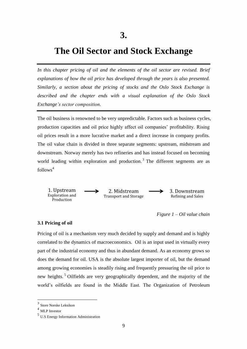
The oil value chain is divided in three separate segments: upstream, midstream and
downstream. Norway merely has two refineries and has instead focused on becoming
world leading within exploration and production.3 The different segments are as
follows4
Figure 1 – Oil value chain
3.1 Pricing of oil
Pricing of oil is a mechanism very much decided by supply and demand and is highly
correlated to the dynamics of macroeconomics. Oil is an input used in virtually every
part of the industrial economy and thus in abundant demand. As an economy grows so
does the demand for oil. USA is the absolute largest importer of oil, but the demand
among growing economies is steadily rising and frequently pressuring the oil price to
new heights. 5
Oilfields are very geographically dependent, and the majority of the
world’s oilfields are found in the Middle East. The Organization of Petroleum
3 Store Norske Leksikon
4 MLP Investor
5 U.S Energy Information Administration
1. Upstream Exploration and
Production
2. Midstream Transport and Storage
3. Downstream Refining and Sales

10
Exporting Countries (OPEC) consists of twelve countries and controls the production
of oil in the Middle East. The purpose of OPEC is to stabilize the oil market and
guarantee high returns to all member countries. The oil production among OPEC
members is sufficient enough to influence the oil pricing through their supply
policies.6
Oil is one of the most important sources of energy in the world. The high dependency
on oil results in an extremely inelastic short-run demand curve. The short-run supply
of oil is limited and the refining process long, also resulting in an inelastic supply
curve.
Figure 2 shows the effect of a positive demand shock for oil when both demand and
supply are inelastic.7 The demand curve shifts from D1 to D2, and evidently changes
in demand result in large price and small quantity changes.
This is the case in the short-run, however, in a longer perspective advances in
technology will alter this slightly since there will be new and more effective ways of
refining oil. Substitutes for oil will slowly transfer energy demand away from oil and
consequently force the demand curve to become more elastic.
6 Rousseau 1998, p. 1
7 Economist help
Q1 Q2
Price
Quantity
P1
P2
D1
D2
S1
Figure 2 – Oil supply and demand
curve
S=Supply
D=Demand
P=Price
Q=Quantity
11
3.2 Oil price development
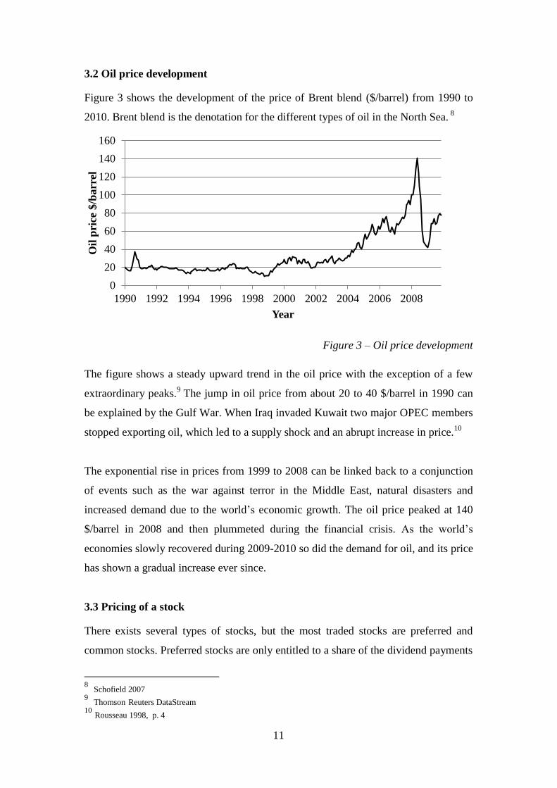
Figure 3 shows the development of the price of Brent blend ($/barrel) from 1990 to
2010. Brent blend is the denotation for the different types of oil in the North Sea. 8
Figure 3 – Oil price development
The figure shows a steady upward trend in the oil price with the exception of a few
extraordinary peaks.9 The jump in oil price from about 20 to 40 $/barrel in 1990 can
be explained by the Gulf War. When Iraq invaded Kuwait two major OPEC members
stopped exporting oil, which led to a supply shock and an abrupt increase in price.10
The exponential rise in prices from 1999 to 2008 can be linked back to a conjunction
of events such as the war against terror in the Middle East, natural disasters and
increased demand due to the world’s economic growth. The oil price peaked at 140
$/barrel in 2008 and then plummeted during the financial crisis. As the world’s
economies slowly recovered during 2009-2010 so did the demand for oil, and its price
has shown a gradual increase ever since.
3.3 Pricing of a stock
There exists several types of stocks, but the most traded stocks are preferred and
common stocks. Preferred stocks are only entitled to a share of the dividend payments
8 Schofield 2007
9 Thomson Reuters DataStream
10 Rousseau 1998, p. 4
0
20
40
60
80
100
120
140
160
1990 1992 1994 1996 1998 2000 2002 2004 2006 2008
Oil
pri
ce $
/barr
el
Year

12
while common stocks typically also have voting rights. The fluctuations in stock
prices can be explained by simple supply and demand. For example, if a large
stakeholder decides to sell his entire share, the market will experience a supply shock
and the stock price will decline due to excess supply.
One of the widely accepted stock pricing models is called the discounted cash flow
model. 11
Typical cash flows received from a stock are dividend payments and the
capital acquired when selling the stock. According to Elton and Gruber (2009)
“discounted cash flow models are based on the concept that the value of a share of
stock is equal to the present value of the cash flow that the stockholder expects to
receive from it”.12
Equation 1 shows how the value of a stock is dependent on the cash
flow at period t (CFt), the discounted rate (r) and the amount of periods the stock
exists (N).
∑
Equation 1 – Pricing of stocks
Companies that are dependent on oil as an input factor (for example the shipping,
aviation, and transport industry) are highly sensitive to changes in oil price. Higher
prices result in higher costs and consequently lower profits. A dividend payment is
defined as the portion of the corporate profits paid back to the company stakeholders,
thus lower profits would shrink dividend payments and investors cash flow
accordingly.13
Companies that, on the other hand, produce and sell oil (output factor)
will experience the complete opposite effect.
3.4 Oslo Stock Exchange
King Carl Johan of Norway officially opened Christiania Exchange, now known as
Oslo Stock Exchange, in April 1819. Its main purpose was to enable the trade of
exchange rates. It was not until the beginning of the 20th
century it became an
exchange for commodities with listed prices for various goods. On 1 March 1881 the
11
Graham et al. 2010, p. 140 12
Elton et al. 2009, p 396-427 13
Business dictionary

13
first ever list of prices for 16 bonds and 23 shares was published, and is regarded as
the date of origin of the modern Norwegian equity market.14
The index used in this
study is the Oslo Exchange Benchmark – Total Return Index (OSEBX). The index
functions as an indicator of the performance of the Oslo Stock Exchange and has a
base value of 100 on the 31st of Dec 1995.
15
Figure 4 – Oslo Stock Exchange development
Figure 4 shows the development on the Oslo Stock Exchange between 1990-2011.
The stock exchange showed a steady upward trend through the 90s with the exception
of the dip in 1998. During 2000-2003 the stock market lost half its value, which can
largely be explained by the dotcom-bubble. However, the market quickly recovered
and experienced an astonishing exponential growth all the way through 2007 and
peaked at all-time-high 510 points. When the financial crisis hit in late 2007, oil
prices as well as the stock market plummeted by more than 50%.
Norway has become one of the world leading countries in production and exportation
of oil and gas, which has resulted in a substantial growth of the energy sector. Further,
Statoil is the largest company within the energy sector and has one fourth of the total
stock exchange market value.16
With the energy sector expanding and increasing its
share of the total market value, the stock exchange should have become more exposed
to fluctuations in oil and gas prices and exports.
14
Oslo Stock Exchange 15
Bloomberg 16
Statoil
0
100
200
300
400
500
600
1990 1992 1994 1996 1998 2000 2002 2004 2006 2008 2010
Po
ints
Year

14
3.4.1 Sector Composition
Stock exchanges are usually built up by several smaller sectors. Depending on the
characteristics of the companies they get divided into similar groups, so called sectors.
In this paper the companies have been divided by the international standard GICS
(Global Industry Classification Standard) developed by Standard & Poor.17
The
energy sector approximately aggregates to half of Oslo Stock Exchange’s market
value, and thus plays a huge role in the Norwegian economy. Within the energy sector
we find companies that expertise in the construction of oilrigs, drilling equipment,
and other related services. Research and exploration activities, production, refining
and transport of oil and gas products are also included.
Knowledge regarding the development of the sector composition is essential when
understanding the stock exchange’s economic function. When evaluating the effect of
a change in oil price on the Oslo Stock Exchange, it is important to know how large
the proportion of companies related to the oil industry is.
Figure 5 – Sector composition
The Oslo Stock Exchange consists of 45.17 percent energy related companies.18
Oil,
as a major contributive factor to these companies’ profits, should therefore have a
significant impact on the companies’ stock performance.
17
Oslo Stock Exchange 2010 18
Ibid.
6,05%
4,16%
45,17%
1,30%
11,73%
0,85%
8,29%
2,44%
10,22%
8,83% 0,97% Consumer Discretionary
Consumer Staples
Energy
Equity Certificates
Financials
Health Care
Industrials
Information Technology
Materials
Telecommunication Services
Utilities
15
4.
Regression parameters
In this chapter all the regression parameters are specified. The choice of regression
parameters is reasoned for and explained. A thorough description of all the variables
is given and discussions of how they ought to affect the Oslo Stock Exchange are held.
Modeling the Oslo Stock Exchange against merely oil price would generate serious
estimation complications due to Omitted Variable Bias (OVB). According to Barreto
and Howland (2006), OVB arises when the relationship between two variables is
explained, but important variables that correlate and, or have a significant relationship
with the dependent variable are excluded.19
It is therefore crucial to include other
explanatory variables to avoid such a bias. We have used a number of explanatory
variables when trying to explain as much variation as possible on the Oslo Stock
Exchange. We have chosen the variables with regard to previous research and
economic theory. Our regression model consists therefore of eight explanatory
variables and is shown below
iceOilPSFTSE
GBPNOKUSDNOKRateInterestGDPCPIOSEBX
Pr500&100
//
987
654321
Δ = Percentage Change
OSEBX = Oslo Stock Exchange – Benchmark Index
CPI = Consumer Price Index
GDP = Gross Domestic Product
NOK/USD = Exchange rate US Dollars and Norwegian Krone
NOK/GBP = Exchange rate British Pound and Norwegian Krone
FTSE 100 = 100 largest stocks on the London Stock Exchange
S&P 500 = 500 largest stocks on the New York Stock Exchange and NASDAQ
Equation 2 – Regression model
4.1 Dependent variable
Data for the stock market have been collected quarterly from Thomson Reuters
Datastream and estimated as quarterly price differences in percent. Data from the first
quarter of 1990 to the last quarter of 2009 have been used.
19
Barreto et al. 2006, p. 493
16
4.2 Explanatory variables
4.2.1 Gross Domestic Product
Gross domestic product (GDP) measures the value of all goods and services produced
within a country during a specific time period, and is calculated using the following
formula20
GDP = Private consumption + Industry investments+ Government spending + Export
– Imports
Equation 3 – Gross Domestic Product
We have used quarterly GDP values starting 1 January 1990 from the Norwegian
Central Bureau of Statistics in the regression. All values are measured in 2009 price
levels.
4.2.2 Interest rate
The Norwegian interest rate is set by the Central Bank of Norway. An increase in the
interest rate makes it more expensive for banks to borrow money, which again leads
to higher borrowing costs for the individual consumer. Essentially, it becomes more
attractive to save than to spend money. Companies are also affected since it becomes
more expensive to take loans and invest, which will lead to lower profits.21
This could
lower the stock prices for the companies since their estimated cash flow will go down.
Low interest rates result in more money being pushed into the economy. More money
will be spent which will further lead to more investments and larger company profits.
Low interest rates thus have a positive effect on the stock market as companies
increase their future estimated cash flows. A consequence of low interest rate can be
high inflation as more money circulates in the economy.22
In calculating the interest
rates between 1990-2009 we have used quarterly data from the Central Bank of
Norway.
20
Swedbank 21
Ibid. 22
Ibid.
17
4.2.3 Inflation
In an economy, inflation measures the rise in general price level and is measured
using consumer price index (CPI). To calculate CPI, the price of a basket of goods
and services is each month compared to the very same basket as the month before. 23
Inflation arises when there is too much money chasing too few goods in the
economy.24
Inflation results in future income being worth less and thus has a negative
effect on companies’ stock performance. For this reason inflation ought to have a
negative effect on our dependent variable. We have used quarterly CPI data from the
Norwegian Central Bureau of Statistics.
4.2.4 Oil
Oil is an important input factor to the industrial sector and on the contrary an output
factor to most of the energy sector. Changes in the price of oil ought to have a direct
effect on companies’ current and future cash flows and therefore affect the stock
performance. An increase in the oil price would significantly increase the industrial
sector’s production costs and thus lower profit margins. On the other hand it would
generate higher revenues to oil companies within the energy sector. The energy sector
accounts for 45.17 percent of the total Oslo Stock Exchange market value, and thus
fluctuations in the oil price should be apparent in the stock market’s performance.
Further, the oil price is defined as Brent Blend 1 Month Future and has been collected
quarterly from Thomson Reuters DataStream.
4.2.5 FTSE 100 and S&P 500
Norway is considered a small economy highly dependent on export of raw materials
and semi-processed goods such as oil, fish, minerals and forestry. 25
The international
demand for Norwegian exports majorly affects the domestic economy. In order to
capture this variation the two major stock indices S&P 500 (New York Stock
Exchange and NASDAQ) and FTSE 100 (London Stock Exchange) are included as
variables to represent the world’s demand. Well performing stock indices indicate
booming economies with high demand for local as well as foreign goods. In later
23
Riksbanken 24
Swedbank 25
CIA World Factbook

18
years globalization has become a vital part of economics and the stock exchanges are
now interlinked more than ever. International trade, technology transfers and capital
flow between economies have created strong relationships.
OSEBX FTSE 100 S&P 500 TOPIX CHSCOMP
OSEBX 1
FTSE 100 0,73 1
S&P 500 0,50 0,52 1
TOPIX 0,47 0,46 0,42 1
CHSCOMP 0,15 0,09 0,19 0,07 1
Table 1.Correlation matrix between Oslo, London, USA, Tokyo and Shanghai stock indices (1990.01 – 2010.01).
The correlation matrix above shows that FTSE 100 and S&P 500 are highly correlated
with the Oslo Stock Exchange. 26
We have also calculated the correlation between the
Oslo Stock Exchange and Tokyo Stock Exchange (TOPIX) as well as Shanghai Stock
Exchange (CHSCOMP). Since both showed lower correlation with the Oslo Stock
Exchange we decided to exclude them from the regression analysis and only include
FTSE 100 and S&P 500.
4.2.6 Exchange rate NOK/USD and NOK/GBP
All large oil transactions take place in dollars.27
This means that Norwegian
companies that have cash flows in NOK will be sensitive to changes in the exchange
rate. Kaneko and Lee (2005) found, in their study on the Japanese stock market, the
relationship between the stock exchange and the exchange rate to be significant. For
these reasons we have decided to include NOK/USD as a variable to capture the
impact on companies’ profits.
London is known to be the financial center of Europe. London Stock Exchange has a
high liquidity and is therefore an arena for large transactions which many other stock
markets are unable to perform. Great Britain accounts for 26.7 % of Norwegian
exports and is thus Norway´s largest export partner.28
Trades are often made in
Pound/Kroner or Kroner/Pound which makes the exchange rate between the two an
essential part of the Norwegian economy.
26
Reuters Datastream 27
The Guardian 28
CIA World Factbook
19
5.
Modeling
Chapter 5 explains the theory behind the regression model used. All of the conditions
for the model are stated and the possible sources of error are elaborated. Detailed
procedures of how to correct for all possible sources of errors in our regression are
thoroughly explained.
When choosing a model to use we have revised several different types of models in
order to find an appropriate one. VAR-models, factor analysis and linear regressions
are some of the approaches discussed. We have based our decision upon the
econometric courses we have studied up until now. During these courses the focus has
been on linear regressions estimated with ordinary least square, and therefore we have
decided to follow a similar approach. With this method we have the appropriate
knowledge and expertise to conduct the regressions needed to investigate our research
question.
5.1 Multiple linear regression
When estimating relationships between different variables, linear regressions can be
an appropriate method to use. In the case of several explanatory variables, a multiple
linear regression must be used.
iikkiii exxxy 123121 ...
Equation 4 – Multiple Linear Model
i denotes the gradient and xki the explanatory variables. The interpretation of the i
-coefficients are made under a strict ceteris paribus condition.29
The purpose of using
a multiple linear regression is to capture as much variation as possible in the
dependent variable through the explanatory variables. It is important to base the
29
Westerlund 2005, p. 138

20
choice of such variables upon previous research and economic theory in order to
attain an appropriate model.
5.2 Ordinary Least Square
In order to estimate the i -coefficients we have used an OLS (Ordinary Least
Squares) estimator. OLS models choose i in a way that minimizes the sum of
squared distances from the predicted line and the observed values ix and iy .30
For this method to be valid a number of conditions must be satisfied31
1) The dependent variable is a linear function of the explanatory variables.
iikkiii exxxy 123121 ...
Equation 5 – OLS condition 1
2) The expected value of the residuals equals zero.
0ieE
Equation 6 - OLS condition 2
3) The residuals are homoscedastic, meaning that they have the same variance
for every i.
2ieVar
Equation 7 - OLS condition 3
4) The covariance between ie and je is zero for every (i,j) and thus the residuals
are uncorrelated.
jiifeeCov ji 0,
Equation 8 - OLS condition 4
5) kix is not random and there is no exact linear relationship between the x-
variables.
30
Ibid. p. 75 31
Ibid. p. 140

21
6) The residuals follow a normal distribution with the expected value 0 and
variance 2 .
2,0 Nei
Equation 9 - OLS condition 6
5.3 Sources of error
If conditions one to five are satisfied, OLS is the most efficient estimator. In order to
use OLS and make correct interpretations of the regression the sixth condition must
also be satisfied. We have tested for all six sources of error and corrected them where
appropriate.
5.3.1 Homoscedasticity
If condition 3 is not satisfied the residuals are heteroscedastic. In other words the
variance for the residuals is not constant. In such cases OLS is no longer the best and
most efficient estimator for the regression, and correct inference and confidence
intervals will no longer be possible.32
To examine if the residuals are heteroscedastic,
plot the residuals against each x-variable and look for systematic variation amongst
the spread of the observations. If a systematic variation is evident the residuals are
heteroscedastic. A more accurate way of examining the residuals is to perform a
Goldfeld-Quandts- or a Whites test. The difference between the two test methods is
that the Goldfeld-Quandts test only can discover proportional heteroscedasticity
whilst Whites test can discover all kinds of heteroscedasticity. We have therefore used
Whites test when testing for condition three.33
The test states following hypothesizes
H0: Homoscedastic residuals
H1: Heteroscedastic residuals
Starting with the multiple linear regression model
iikkiii exxxy 123121 ...
Equation 10 – Multiple Linear Model
32
Ibid. p. 173ff 33
Ibid. p. 180f
22
we can estimate the coefficients and calculate the residuals. The following equation is
attained
iikkiikiii uxxxe
2
1
22
12121
2......ˆ
Equation 11 – Whites test: residuals
where ui is an error term and αi are slope coefficients. If, when estimating the new
equation, all slope coefficients equal zero we are merely left with the intercept and
error term .1
2
ii ue In a calculation of the variance we then have
KN
N
kNkN
u
kN
u
kN
eN
i
N
i
N
i
i
N
i
i
N
i
i
11
1
1 1
1
1
1
1
2
2
ˆ
ˆ
Equation 12 – Whites test: variance
since 0iu and 1 is a constant. As can be seen in equation 12 the variance is
constant and the residuals are homoscedastic. If at least one of the slope coefficients
equal any other value than zero the residuals are heteroscedastic.34
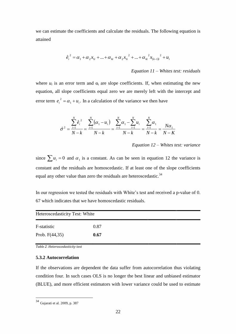
In our regression we tested the residuals with White’s test and received a p-value of 0.
67 which indicates that we have homoscedastic residuals.
Heteroscedasticity Test: White
F-statistic 0.87
Prob. F(44,35) 0.67
Table 2. Heteroscedasticity test
5.3.2 Autocorrelation
If the observations are dependent the data suffer from autocorrelation thus violating
condition four. In such cases OLS is no longer the best linear and unbiased estimator
(BLUE), and more efficient estimators with lower variance could be used to estimate
34
Gujarati et al. 2009, p. 387
23
the regression coefficients. To test for autocorrelation, graphically examine the
residuals against time and look for systematic variation or use a Durbin Watson test.
Durbin Watson tests are conducted under the hypothesizes
H0: No autocorrelation, ρ=0
H1: Autocorrelation ρ > 0
The alternative hypothesis tests for positive autocorrelation since it is the most
common kind of autocorrelation. By using the residuals from our multiple linear
regression we can calculate the Durbin Watson-statistic
)ˆ1(2
ˆ211
ˆ
ˆˆ
2
ˆ
ˆ
ˆ
ˆ
ˆ
ˆˆ2ˆˆ
ˆ
ˆˆ
1
2
2
1
1
2
2
2
1
1
2
2
2
1
2
2 2 2
1
2
1
2
1
2
2
2
1
N
i
i
N
i
ii
N
i
i
N
i
i
N
i
i
N
i
i
N
i
i
N
i
N
i
N
i
iiii
N
i
i
N
i
ii
e
ee
e
e
e
e
e
eeee
e
ee
DW
Equation 13 – Durbin Watson test
If 0ˆ the DW-statistic is approximately 2 and indicates no autocorrelation. If the
regression suffers from positive autocorrelation on the other hand, the DW-statistic
would be close to 0. The DW-value is compared to two critical values (Dupper and
Dlower) to decide whether or not to discard the null hypothesis.35
If DW > Dupper the null hypothesis cannot be rejected
If DW < Dlower the null hypothesis is rejected
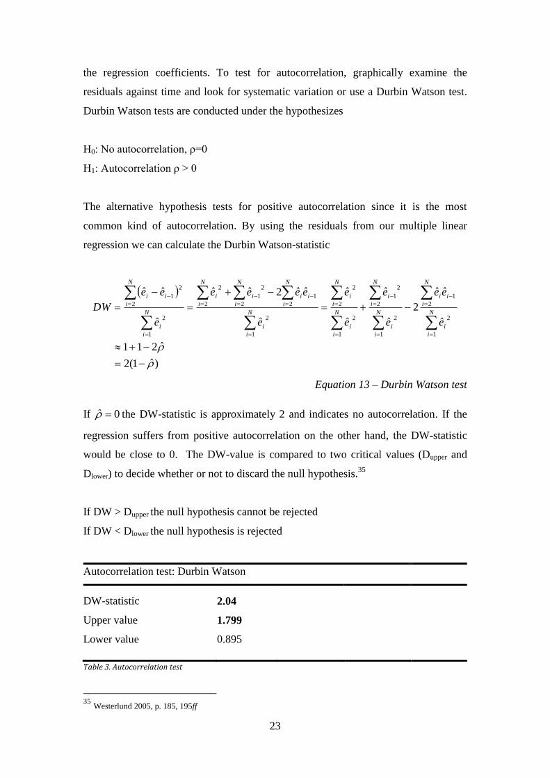
Autocorrelation test: Durbin Watson
DW-statistic 2.04
Upper value 1.799
Lower value 0.895
Table 3. Autocorrelation test
35
Westerlund 2005, p. 185, 195ff
24
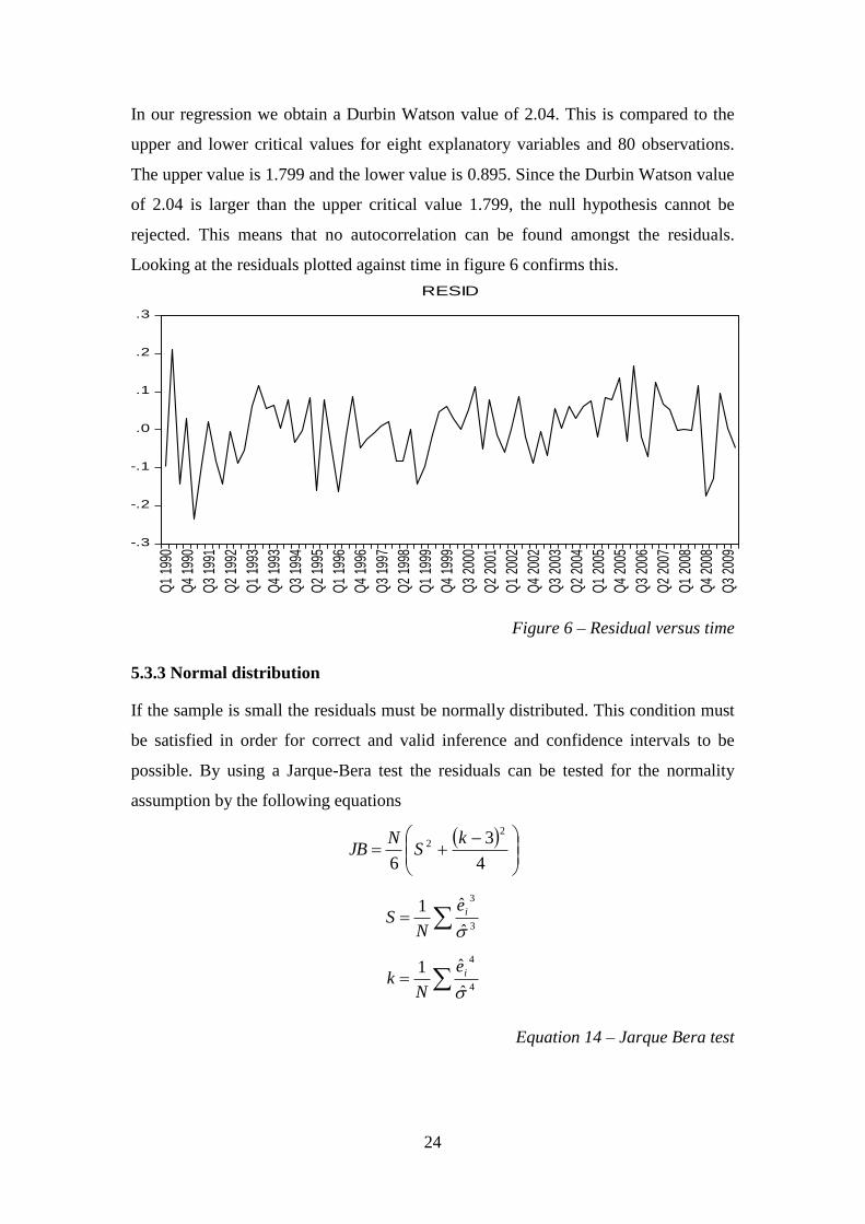
In our regression we obtain a Durbin Watson value of 2.04. This is compared to the
upper and lower critical values for eight explanatory variables and 80 observations.
The upper value is 1.799 and the lower value is 0.895. Since the Durbin Watson value
of 2.04 is larger than the upper critical value 1.799, the null hypothesis cannot be
rejected. This means that no autocorrelation can be found amongst the residuals.
Looking at the residuals plotted against time in figure 6 confirms this.
Figure 6 – Residual versus time
5.3.3 Normal distribution
If the sample is small the residuals must be normally distributed. This condition must
be satisfied in order for correct and valid inference and confidence intervals to be
possible. By using a Jarque-Bera test the residuals can be tested for the normality
assumption by the following equations
4
3
6
2
2 kS
NJB
3
3
ˆ
ˆ1
ie
NS
4
4
ˆ
ˆ1
ie
Nk
Equation 14 – Jarque Bera test
-.3
-.2
-.1
.0
.1
.2
.3
Q1
1990
Q4
1990
Q3
1991
Q2
1992
Q1
1993
Q4
1993
Q3
1994
Q2
1995
Q1
1996
Q4
1996
Q3
1997
Q2
1998
Q1
1999
Q4
1999
Q3
2000
Q2
2001
Q1
2002
Q4
2002
Q3
2003
Q2
2004
Q1
2005
Q4
2005
Q3
2006
Q2
2007
Q1
2008
Q4
2008
Q3
2009
RESID

25
where S is a measurement for skewness of the residuals’ probability distribution and k
measures the kurtosis of the probability distribution. If the condition is satisfied, S
will be close to zero and k will be close to three. The test statistic should therefore be
close to zero in order for the normality condition to be fulfilled. 36
In our regression we obtained a JB-value of 0.95, which should be compared to
appropriate critical values. However, the test also provides us with a p-value and
needs only be compared to a chosen confidence level. In our regression we received a
p-value of 0.62 which indicates that the residuals fulfill the assumption of normality.
Figure 7 – Normality test
5.3.4 Multicollinearity
When estimating a model using more than one explanatory variable, the possibility of
multicollinearity arises. When two variables are highly correlated, it can be difficult
to separate their individual effects on the dependent variable since they virtually
contain the same information. In models with multicollinearity, high variance and
covariance is a common problem. As a result deciding which signs the regression
coefficients should have become difficult. High R2-values together with few
significant t-statistics is a typical indication of multicollinearity. When obtaining high
R2-values, all F-tests constructed will likely reject the null-hypothesis indicating that
the regressions slope coefficients equals zero, meaning that the t-statistics should be
significant. This will not be the case if the degree of multicollinearity is high since
most t-statistics will be non-significant. To correct for multicollinearity, one of the
correlated variables can be discarded without causing the determination coefficient to
36
Ibid. p. 134f
0
2
4
6
8
10
12
14
-0.2 -0.1 0.0 0.1 0.2
Series: ResidualsSample 1 80Observations 80
Mean 2.20e-16Median 0.000920Maximum 0.212570Minimum -0.233923Std. Dev. 0.084507Skewness -0.268155Kurtosis 2.999184
Jarque-Bera 0.958761Probability 0.619167

26
drop significantly. Although, one should be careful when excluding variables from the
regression as the regression may become biased. 37
Multicollinearity is discussed in matters of degrees and not in matters of testing for its
existence. To test the degree of multicollinearity in a regression, a variance inflation
factor test (VIF) can be used. First, investigate the co-linearity between the x-
variables by estimating regressions where each explanatory variable act as a
dependent variable against the other explanatory variables. These equations are called
subsidiary regressions. 38
In our paper we get seven different subsidiary regressions
since we have eight explanatory variables.
iiiiiiii uxxxxxxxx 8877665544332211
iiiiiiii uxxxxxxxx 8877665544331112
iiiiiiii uxxxxxxxx 8877665544221113
iiiiiiii uxxxxxxxx 8877665533221114
iiiiiiii uxxxxxxxx 8877664433221115
iiiiiiii uxxxxxxxx 8877554433221116
iiiiiiii uxxxxxxxx 8866554433221117
iiiiiiii uxxxxxxxx 7766554433221118
Equation 15 – Subsidiary equations
To calculate VIF-values for each regression we used equation 16 where the
coefficient of determination was received from each subsidiary regression.
21
1
i
iR
VIF
Equation 16 – VIF
37
Gujarati 2006, p. 371ff 38
Ibid.
27
xi R2-value VIF-value
CPI 0.07 1.08
GDP 0.18 1.21
Interest rate 0.40 1.68
Oil 0.45 1.81
NOK/GBP 0.38 1.61
NOK/USD 0.37 1.60
FTSE 100 0.67 3.04
S&P 500 0.68 3.15
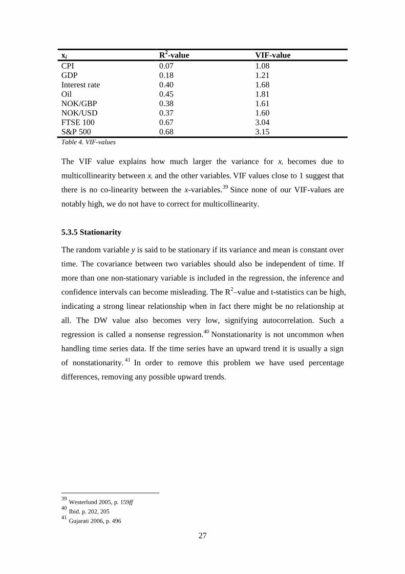
Table 4. VIF-values
The VIF value explains how much larger the variance for xi becomes due to
multicollinearity between xi and the other variables. VIF values close to 1 suggest that
there is no co-linearity between the x-variables.39
Since none of our VIF-values are
notably high, we do not have to correct for multicollinearity.
5.3.5 Stationarity
The random variable y is said to be stationary if its variance and mean is constant over
time. The covariance between two variables should also be independent of time. If
more than one non-stationary variable is included in the regression, the inference and
confidence intervals can become misleading. The R2–value and t-statistics can be high,
indicating a strong linear relationship when in fact there might be no relationship at
all. The DW value also becomes very low, signifying autocorrelation. Such a
regression is called a nonsense regression.40
Nonstationarity is not uncommon when
handling time series data. If the time series have an upward trend it is usually a sign
of nonstationarity.41
In order to remove this problem we have used percentage
differences, removing any possible upward trends.
39
Westerlund 2005, p. 159ff 40
Ibid. p. 202, 205 41
Gujarati 2006, p. 496
28
6.
Results and analysis
In chapter 6 our results are presented and analyzed. When testing for the period
1990-2009 it can be proven that oil has a significant effect on the Oslo Stock
Exchange return. To investigate this in more detail, a moving average process and
two separate regressions where executed for two sub-periods, 1990-1999 and 2000-
2009. Possible reasons and explanations for the results are discussed and analyzed.
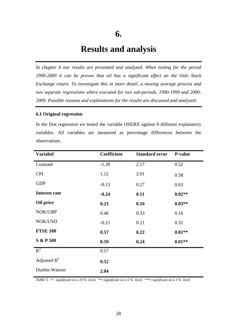
6.1 Original regression
In the first regression we tested the variable OSEBX against 8 different explanatory
variables. All variables are measured as percentage differences between the
observations.
Variabel Coefficient Standard error P-value
Constant -1.39 2.17 0.52
CPI 1.12 2.01 0.58
GDP -0.13 0.27 0.63
Interest rate -0.24 0.11 0.02**
Oil price 0.23 0.10 0.03**
NOK/GBP 0.46 0.33 0.16
NOK/USD -0.21 0.21 0.32
FTSE 100 0.57 0.22 0.01**
S & P 500 0.59 0.24 0.01**
R2
0.57
Adjusted R2
0.52
Durbin-Watson 2.04
Table 5 . *= significant on a 10 % -level, **=significant on a 5 % -level, ***=significant on a 1 % -level

29
As shown in table 5, four of the eight explanatory variables proved to be significant
on a 5 percent significance level. Interest rate, oil, FTSE 100 and S&P 500 did all
show significant effects on OSEBX.
The R2-value indicates how much of the total variation in the dependent variable that
can be explained by the explanatory variables. This measurement does not consider
the number of explanatory variables used in the regression and may thus lead to a
misleading conclusion. The R2-adjusted value, however, is a much more accurate
measurement as it takes the number of explanatory variables into account.
Variabel Coefficient Standard error P-value
Interest rate -0.24 0.11 0.02**
Oil price 0.23 0.10 0.03**
FTSE 100 0.57 0.22 0.01**
S&P 500 0.59 0.24 0.01**
Table 6. *= significant on a 10 % -level, **=significant on a 5 % -level, ***=significant on a 1 % -level
Since all observations are percentage differences, the interpretation of the regression
coefficients will be in percentages. FTSE 100 has a coefficient equal to 0.57 which
means that a one-percentage increase on the London Stock Exchange will lead to a
0.57 percent increase on the Oslo Stock Exchange. S&P 500 also has a positive effect
on the Oslo Stock Exchange, as its regression coefficient is 0.59. The reason for the
positive correlations between the stock markets leads to the argument of economic
globalization. There is more and more profound proof of the fact that events in large
country’s economy also affect smaller economies. Free trade agreements, larger
capital flows and technology and labor transfers have created strong relationships
between countries, which leads to a more integrated world economy.
The interest rate displays a negative effect on the Oslo Stock Exchange. The
regression coefficient of -0.24 indicates that a one-percentage increase of the interest
rate leads to a 0.24 percentage decrease on the Oslo Stock Exchange. This is in
agreement with our hypothesis from previous chapters. When the central bank
increases the interest rate it becomes more expensive for banks to loan money.
Consequently banks increase their own borrowing rate and individuals and companies
30
tend to postpone investments until funding becomes cheaper. This results in a lower
aggregate demand. Referring back to the future cash flow model, such an event will
affect the stock market as the stock price is set by the future cash flow of the company.
When a company cuts back on investments and spending it will consequently
decrease future cash flow and therefore lower the stock price.
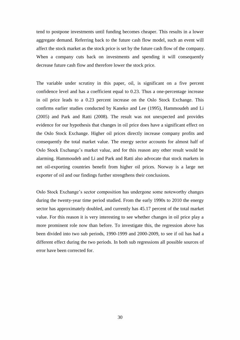
The variable under scrutiny in this paper, oil, is significant on a five percent
confidence level and has a coefficient equal to 0.23. Thus a one-percentage increase
in oil price leads to a 0.23 percent increase on the Oslo Stock Exchange. This
confirms earlier studies conducted by Kaneko and Lee (1995), Hammoudeh and Li
(2005) and Park and Ratti (2008). The result was not unexpected and provides
evidence for our hypothesis that changes in oil price does have a significant effect on
the Oslo Stock Exchange. Higher oil prices directly increase company profits and
consequently the total market value. The energy sector accounts for almost half of
Oslo Stock Exchange’s market value, and for this reason any other result would be
alarming. Hammoudeh and Li and Park and Ratti also advocate that stock markets in
net oil-exporting countries benefit from higher oil prices. Norway is a large net
exporter of oil and our findings further strengthens their conclusions.
Oslo Stock Exchange’s sector composition has undergone some noteworthy changes
during the twenty-year time period studied. From the early 1990s to 2010 the energy
sector has approximately doubled, and currently has 45.17 percent of the total market
value. For this reason it is very interesting to see whether changes in oil price play a
more prominent role now than before. To investigate this, the regression above has
been divided into two sub periods, 1990-1999 and 2000-2009, to see if oil has had a
different effect during the two periods. In both sub regressions all possible sources of
error have been corrected for.

31
6.1.1 Sub-period 1: 1990-1999
Variabel Coefficient Standard error P-value
Constant 4.17 4.41 0.35
CPI -4.37 4.00 0.28
GDP 0.11 0.47 0.82
Interest rate -0.51 0.14 0.0007***
Oil price 0.45 0.14 0.0031***
NOK/GBP 0.16 0.45 0.73
NOK/USD 0.64 0.31 0.04**
FTSE 100 0.45 0.25 0.08*
S & P 500 -0.06 0.37 0.87
R2
0.60
Adjusted R2
0.49
Durbin-Watson 2.05
Table 7. *= significant on a 10 % -level, **=significant on a 5 % -level, ***=significant on a 1 % -level
In the regression for the period 1990-1999 the same four explanatory variables proved
to be significant except for S&P 500 that has been replaced by NOK/USD. The
adjusted R2-value decreased to 0.49 and the regression explains less of the variation in
OSBEX than the first. Interest rate is significant on a 1 %-level which is a higher level
than in the previous regression. On the other hand FTSE 100 is now significant on a
10%-level compared to its previous 5 %-level, indicating that it explains a smaller
part of the variation in OSBEX during 1990-1999 than 1990-2009. The variable oil is
now significant on a 1 %- level and yields the coefficient 0.45, which means that a
one-percentage increase in oil prices leads to an increase of 0.45 percent on the Oslo
Stock Exchange. When comparing this value to the regression covering the entire
period, it is evident that changes in oil prices had a bigger effect on the Oslo Stock
Exchange in 1990-1999. These results agree with our hypothesis and previous results
and are in no way surprising.
A noteworthy change for this period is the variable NOK/USD. The exchange rate is
now significant on a 5 %-level. Since USA is a major export partner for Norway, such
32
a result was to be expected. Between 1990 and 2000 Norwegian exports to the USA
more than doubled from $2152 million to $4553 million. During this time they
substantially increased their exposure to dollars, explaining its significance. 42
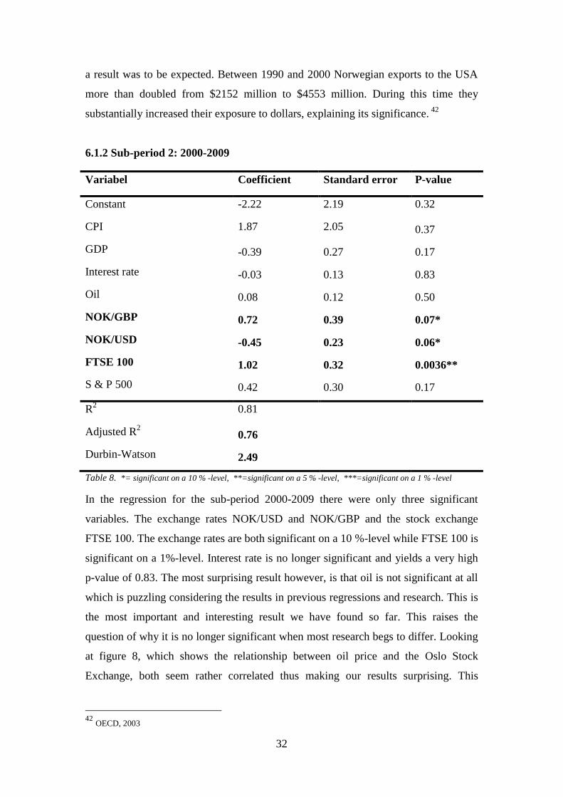
6.1.2 Sub-period 2: 2000-2009
Variabel Coefficient Standard error P-value
Constant -2.22 2.19 0.32
CPI 1.87 2.05 0.37
GDP -0.39 0.27 0.17
Interest rate -0.03 0.13 0.83
Oil 0.08 0.12 0.50
NOK/GBP 0.72 0.39 0.07*
NOK/USD -0.45 0.23 0.06*
FTSE 100 1.02 0.32 0.0036**
S & P 500 0.42 0.30 0.17
R2
0.81
Adjusted R2
0.76
Durbin-Watson 2.49
Table 8. *= significant on a 10 % -level, **=significant on a 5 % -level, ***=significant on a 1 % -level
In the regression for the sub-period 2000-2009 there were only three significant
variables. The exchange rates NOK/USD and NOK/GBP and the stock exchange
FTSE 100. The exchange rates are both significant on a 10 %-level while FTSE 100 is
significant on a 1%-level. Interest rate is no longer significant and yields a very high
p-value of 0.83. The most surprising result however, is that oil is not significant at all
which is puzzling considering the results in previous regressions and research. This is
the most important and interesting result we have found so far. This raises the
question of why it is no longer significant when most research begs to differ. Looking
at figure 8, which shows the relationship between oil price and the Oslo Stock
Exchange, both seem rather correlated thus making our results surprising. This
42
OECD, 2003

33
indicates that there is an underlying factor affecting both oil prices and the stock
market which our model has not been able to capture.
Figure 8 – Oil price and stock prices
The energy sector has seen a substantial growth during the second sub-period, at the
same time the composition of the Oslo Stock Exchange has also changed. The stock
exchange can in fact be explaining a lot of its own variation, making oil price changes
play a smaller role than before.43
Another very important notation is the changes
made in the Norwegian oil industry. Norway has in the last decade focused more on
intelligence and technology research within the oil industry, than on refining crude oil.
There are only two refineries left in Norway today and most oil is sent abroad as
crude oil and later imported as refined products. Therefore the Norwegian economy
has diversified its exposure to oil price changes and spread the risks within the entire
oil industry.
6.1.3 Moving Average Process
Due to the oil not being significant in the second sub period, we decided to construct a
moving average process in hope of finding specific time points were oil is non-
significant. The moving average process was created by simulating the same
regression but with overlapping time periods, all being four years long. Figure 9
shows the process with the p-values for oil from each regression.
43 See Sadorsky 1999
199
0
199
1
199
2
199
3
199
4
199
5
199
6
199
7
199
8
199
9
200
0
200
1
200
2
200
3
200
4
200
5
200
6
200
7
200
8
200
9
Oil
OSBEX
34
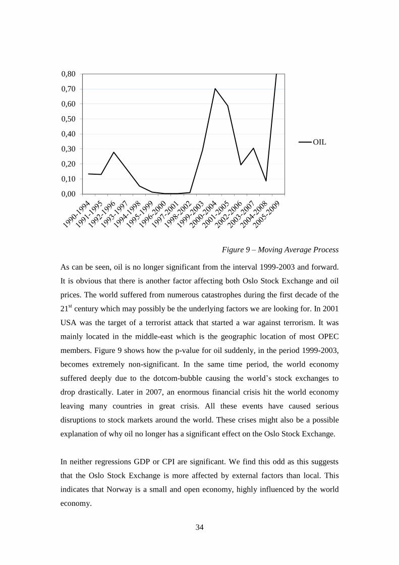
Figure 9 – Moving Average Process
As can be seen, oil is no longer significant from the interval 1999-2003 and forward.
It is obvious that there is another factor affecting both Oslo Stock Exchange and oil
prices. The world suffered from numerous catastrophes during the first decade of the
21st century which may possibly be the underlying factors we are looking for. In 2001
USA was the target of a terrorist attack that started a war against terrorism. It was
mainly located in the middle-east which is the geographic location of most OPEC
members. Figure 9 shows how the p-value for oil suddenly, in the period 1999-2003,
becomes extremely non-significant. In the same time period, the world economy
suffered deeply due to the dotcom-bubble causing the world’s stock exchanges to
drop drastically. Later in 2007, an enormous financial crisis hit the world economy
leaving many countries in great crisis. All these events have caused serious
disruptions to stock markets around the world. These crises might also be a possible
explanation of why oil no longer has a significant effect on the Oslo Stock Exchange.
In neither regressions GDP or CPI are significant. We find this odd as this suggests
that the Oslo Stock Exchange is more affected by external factors than local. This
indicates that Norway is a small and open economy, highly influenced by the world
economy.
0,00
0,10
0,20
0,30
0,40
0,50
0,60
0,70
0,80
OIL
35
7.
Conclusion
In this chapter a summary of our results are presented. The hypothesis in the
beginning of the paper is compared to the final results and suggestions for further
research are given.
The purpose of this paper was to investigate the relationship between changes in oil
price and changes on the Oslo Stock Exchange. The hypothesis of this paper was that
changes in the oil price have significant effects on the stock market due to the energy
sector’s large proportion of the market value.
A multiple linear regression using an OSL estimator was constructed with data
covering a twenty year time period starting with the first quarter of 1990 to the last
quarter of 2009. The model was even divided into two equally long sub periods to
assess whether the effects of changes in the oil price are more prominent now than
before. Several explanatory variables were selected to avoid any omitted variable bias,
and the result was unambiguous. All conditions needed to be fulfilled in order for
OLS to be the best estimator has been corrected for.
After analyzing the entire time period, changes in oil price proved to have a
significant effect on a 5 percent confidence level. One percentage increase in oil
prices would approximately increase the stock exchange by 0.22 percent. Interest rate,
FTSE100 and S&P500 were the only explanatory variables that were significant.
Sadorsky found in 1999 that interest rates had a greater impact than oil shocks, which
also was true in our study. The interest rate had a coefficient of -0.24 compared to
0.22. Our result also strengthens Hammoudeh and Li and Park and Ratti conclusion
that stock markets in net-exporting countries like Norway will be positively affected
by rising oil prices.
When examining the first sub-period it was evident that oil price changes were
significant on a 1 percent confidence level. The coefficient equaled 0.45 which is
approximately double the coefficient compared to when studying the whole twenty-

36
year period. This is quite a notable increase and knowledge of the oil price
development could indeed have been very lucrative. Even during the 90s, interest rate
had a greater impact than changes in oil price, which again agrees with Sadorsky’s
conclusion from 1999.
The result from the second sub-period, however, was startling. Expecting changes in
oil price to have an even greater impact than in the first sub period, it proved not to be
significant at all. Oil had a very high p-value of 0.50 and a rather low coefficient of
0.08. After further analysis of the material we reached the final conclusion that the
stock exchange and oil remain highly correlated, but both seem to be following
another factor our model has not been able to capture. It would be very interesting to
continue this research and find the factor affecting both the stock market and the oil
price.
In our study we chose to include the two most correlated stock exchanges. However,
using factor analysis numerous exchanges can be included without experiencing
multicollinearity problems. Using this method it would be possible to describe a set of
p stock exchanges X1, X2,…, Xp in terms of a smaller number of indices or factors, and
in such a way elucidate the relationship between the stock exchanges. Further we
chose to use a multiple linear regression due to our level of econometric education,
although the vector autoregression (VAR) model is one of the most successful and
flexible models to use for the analysis of multivariate time series. For further research
we would find it interesting to use a VAR model that would allow for direct
comparisons with previous research and more in-depth analysis.

37
8.
References
Barreto, Humberto; Howland, Frank M (2006). Introductory econometrics: Using
Monte Carlo simulation with Microsoft Excel. USA: Cambridge University Press.
Basher, Syed A; Sadorsky, Perry (2004). Oil price risk and emerging stock markets.
In: Global Finance Journal; Elsevier vol. 17 (2). P 224-251.
http://www.syedbasher.org/published/2006_GFJ.pdf (2011-11-11)
Bloomberg
http://www.bloomberg.com/apps/quote?ticker=OSEBX:IND (2011-10-12)
Business Dictionary
http://www.businessdictionary.com/definition/dividend.html (2011-12-21)
Chen, Nai-Fu; Roll, Richard; Ross, Stephen A (1986). Economic forces and the stock
market. In: Journal of Business 59. P. 383−403.
http://rady.ucsd.edu/faculty/directory/valkanov/classes/mfe/docs/ChenRollRoss_JB_1986.pdf (2011-11-11)
CIA World Factbook
https://www.cia.gov/library/publications/the-world-factbook/ge (2001-11-25)
Ciner, Cetin (2001). Energy shocks and Financial Markets: Nonlinear Linkages. In:
Studies in Nonlinear Dynamics and Econometrics, October, 5 (3). P. 203-212.
http://scholar.lib.vt.edu/ejournals/SNDE/snde-mirror/005/articles/v5n3003.pdf (2011-11-11)
Edwin, Elton J; Gruber, Martin J (2009). Modern Portfolio Theory and Investment
Analysis. 8th Edition. USA: John Wiley & Sons.
Graham, John R; Smart, Scott B; Megginson, William L (2010). Corporate Finance:
Linking Theory To What Companies Do. 3d Edition. USA: South-Western Cengage
Learning.
38
Gujarati, Damodar N (2006). Essentials of Econometrics. 3d Edition. USA: McGraw-
Hill/Irwin.
Gujarati, Damodar N; Porter, Dawn C (2009). Basic Econometrics. 5th Edition. USA:
McGraw-Hill/Irwin
Hammoudeh, Shawkat; Li, Huimin (2005). Oil Sensitivity and Systematic Risk in Oil
Sensitive Stock Indices. In: Journal of Economics and Business, Vol. 57. P. 1-21.
http://www.sciencedirect.com/science/article/pii/S0148619504000748 (2011-11-11)
Huang, Roger D; Masukis, Ronald W; Stoll, Hans R (1996). Energy shocks and
financial markets. In: Journal of Futures Markets, vol. 16. P. 1-27.
http://onlinelibrary.wiley.com/doi/10.1002/(SICI)1096-9934(199602)16:1%3C1::AID-FUT1%3E3.0.CO;2-
Q/abstract (2012-01-19)
Jones, Charles M; Kaul, Gautam (1996). Oil and Stock Markets. In: The Journal of
Finance; Elsevier vol. 51 (2). P. 463-491.
http://www.jstor.org/stable/2329368 (2011-11-14)
Kaneko, T; Lee, B. S (1995). Relative importance of economic factors in the U.S. and
Japanese stock markets. In: Journal of the Japanese and International Economies 9.
P. 290−307.
http://econpapers.repec.org/article/eeejjieco/default10.htm (2011-11-12)
MLP Investor
http://www.mlpinvestor.com/mlps-energy/ (2012-01-10)
Norwegian Ministry of Petroleum and Energy.
http://www.regjeringen.no/en/dep/oed/Subject/Oil-and-Gas/norways-oil-history-in-5-minutes.html?id=440538
(2011-11-16)
OECD- Reviews of Regulatory Reform: Norway
http://books.google.se/books?id=vgI6_q98YVkC&pg=PA93&lpg=PA93&dq=trade+partners+for+norway+1990&
source=bl&ots=cBcb_W6SB_&sig=0cCUTgrwvmYWN7nLLr1MBbTEs5Q&hl=sv&sa=X&ei=JsMGT_SAAomF
4gTT4cGdAQ&ved=0CCYQ6AEwAQ#v=onepage&q=trade%20partners%20for%20norway%201990&f=false
(2012-01-06)
39
Oslo Stock Exchange
http://www.oslobors.no/ob_eng/Oslo-Boers/About-us/The-history-of-Oslo-Boers (2011-12-01)
Papapetrou, E (2001). Oil price shocks, stock markets, economic activity and
employment in Greece. In: Energy Economics 23. P. 511−532.
http://econ.ccu.edu.tw/manage/1190950202_a.pdf (2011-11-12)
Park, Junkwook; Ratti, Ronald A (2008). Oil price shocks and stock markets in the
U.S. and 13 European countries. In: Energy Economics 30. P. 2587- 2608.
http://econ.ccu.edu.tw/manage/1190950202_a.pdf (2011-11-14)
Riksbanken
http://www.riksbank.se/templates/Page.aspx?id=30986 (2011-11-25)
Rousseau, David L (1998). History of OPEC
http://cnre.vt.edu/lsg/intro/oil.pdf (2011-11-21)
Sadorsky, Perry (1999). Oil price shocks and stock market activity. In: Energy
Economics; Elsevier, vol. 21 (2). P. 449-469.
Schofield, Neil C (2007). Commodity Derivatives: Markets and Applications.
England: John Wiley & Sons Ltd.
Statoil
http://www.statoil.com/annualreport2010/en/shareholderinformation/pages/shareholderinformation0.aspx
(2012-01-05)
Store Norske Leksikon
http://snl.no/oljeraffinering (2011-11-22)
Swedbank
http://www.swedbank.se/privat/spara-och-placera/aktier/lar-dig-allt-om-aktiehandel/aktieskola/analyser
/index.htm?contentid=OID_518076_SV#Räntans betydelse för konjunkturen (2011-11-25)
http://www.swedbank.se/privat/spara-och-placera/aktier/lar-dig-allt-om-
aktiehandel/aktieskola/analyser/index.htm?contentid=OID_518076_SV#BNP (2012-01-08)
40
The Guardian. US rivals 'plotting to end oil trading in dollars'.
http://www.guardian.co.uk/business/2009/oct/06/oil-us-dollar-threat-to-america (2012-01-13)
Thomson Reuters DataStream
(2011-11-05 – 2011-12-10)
U.S Energy Information Administration.
http://205.254.135.7/dnav/pet/pet_move_impcus_a2_nus_epc0_im0_mbbl_m.htm (2011-11-21)
Westerlund, Joakim (2005). Introduktion till ekonometri. Sverige: Studentlitteratur
AB

41
0.990
0.995
1.000
1.005
1.010
1.015
1.020
1.025
-.3 -.2 -.1 .0 .1 .2 .3
RESID
CP
I
0.85
0.90
0.95
1.00
1.05
1.10
1.15
-.3 -.2 -.1 .0 .1 .2 .3
RESID
GD
P
Appendix
Moving Average Process (p-values)
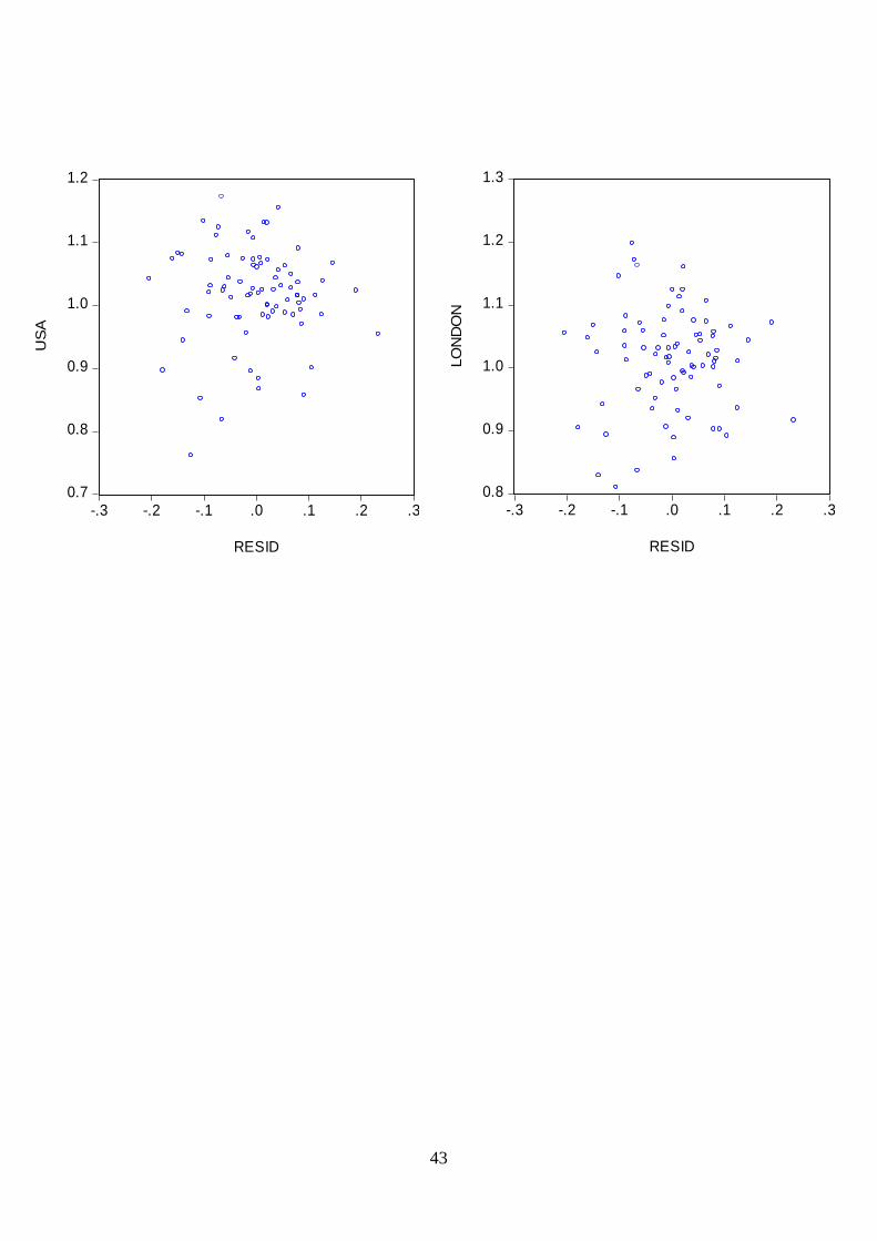
Residual plots of the explanatory variables
Tidsperiod R2-adjusted CPI FTSE100 £/NOK GDP INTEREST RATE OIL S&P500 $/NOK
1990-1994 37,92% 0,1122 0,2961 0,6725 0,03826 0,032 0,1335 0,5162 0,1893
1991-1995 46,32% 0,2105 0,2545 0,6245 0,9859 0,018 0,1302 0,237 0,0821
1992-1996 29,31% 0,5218 0,486 0,8115 0,9269 0,0827 0,2766 0,7554 0,2892
1993-1997 6,11% 0,7177 0,7674 0,4129 0,5425 0,1095 0,1644 0,7862 0,7404
1994-1998 49,51% 0,7063 0,154 0,7542 0,2863 0,0653 0,0525 0,8071 0,6221
1995-1999 57,93% 0,5334 0,0677 0,5918 0,1325 0,0295 0,0105 0,8075 0,5141
1996-2000 72,19% 0,6071 0,0663 0,8011 0,0306 0,0081 0,0013 0,8557 0,1077
1997-2001 84,94% 0,4809 0,1449 0,2566 0,0928 0,0019 0,0008 0,0844 0,0115
1998-2002 79,04% 0,8118 0,1608 0,126 0,3845 0,0196 0,0102 0,1245 0,0842
1999-2003 78,97% 0,9733 0,3167 0,9009 0,3997 0,9472 0,2902 0,0207 0,8355
2000-2004 83,14% 0,8301 0,034 0,6301 0,6792 0,9557 0,7007 0,0609 0,9434
2001-2005 85,47% 0,8341 0,0095 0,4048 0,8826 0,9961 0,5867 0,4913 0,9441
2002-2006 79,29% 0,6118 0,0017 0,4832 0,6112 0,1706 0,1938 0,6206 0,8038
2003-2007 65,04% 0,3537 0,0007 0,4541 0,1878 0,388 0,3045 0,8601 0,8656
2004-2008 70,04% 0,5564 0,0054 0,8287 0,4803 0,5042 0,0875 0,818 0,5943
2005-2009 53,99% 0,6918 0,0733 0,1521 0,2968 0,9939 0,959 0,5639 0,0522

42
0.6
0.7
0.8
0.9
1.0
1.1
1.2
1.3
1.4
1.5
-.3 -.2 -.1 .0 .1 .2 .3
RESID
OIL
0.88
0.92
0.96
1.00
1.04
1.08
1.12
-.3 -.2 -.1 .0 .1 .2 .3
RESID
GB
PN
OK
0.6
0.8
1.0
1.2
1.4
1.6
-.3 -.2 -.1 .0 .1 .2 .3
RESID
Inte
rest
Rate
0.84
0.88
0.92
0.96
1.00
1.04
1.08
1.12
1.16
1.20
1.24
-.3 -.2 -.1 .0 .1 .2 .3
RESID
US
DN
OK
43
0.7
0.8
0.9
1.0
1.1
1.2
-.3 -.2 -.1 .0 .1 .2 .3
RESID
US
A
0.8
0.9
1.0
1.1
1.2
1.3
-.3 -.2 -.1 .0 .1 .2 .3
RESID
LO
ND
ON

44