NBER WORKING PAPER SERIES

OFFSHORING AND UNEMPLOYMENT

Devashish MitraPriya Ranjan

Working Paper 13149http://www.nber.org/papers/w13149

NATIONAL BUREAU OF ECONOMIC RESEARCH1050 Massachusetts Avenue

Cambridge, MA 02138June 2007

We thank seminar participants at Carleton University, Drexel University, the Midwest InternationalTrade Conference in Minneapolis (Spring, 2007), the NBER Spring 2007 International Trade and Investmentgroup meeting, Oregon State University and the World Bank for useful comments and discussions.The views expressed herein are those of the author(s) and do not necessarily reflect the views of theNational Bureau of Economic Research.

© 2007 by Devashish Mitra and Priya Ranjan. All rights reserved. Short sections of text, not to exceedtwo paragraphs, may be quoted without explicit permission provided that full credit, including © notice,is given to the source.

Offshoring and UnemploymentDevashish Mitra and Priya RanjanNBER Working Paper No. 13149June 2007JEL No. E24,F1

ABSTRACT

In this paper, in order to study the impact of offshoring on sectoral and economywide rates of unemployment,we construct a two sector general equilibrium model in which labor is mobile across the two sectors,and unemployment is caused by search frictions. We find that, contrary to general perception, wageincreases and sectoral unemployment decreases due to offshoring. This result can be understood toarise from the productivity enhancing (cost reducing) effect of offshoring. If the search cost is identicalin the two sectors, or even if the search cost is higher in the sector which experiences offshoring, theeconomywide rate of unemployment decreases. We also find multiple equilibrium outcomes in theextent of offshoring and therefore, in the unemployment rate. Furthermore, a firm can increase itsdomestic employment through offshoring. Also, such a firm's domestic employment can be higherthan a firm that chooses to remain fully domestic. When we modify the model to disallow intersectorallabor mobility, the negative relative price effect on the sector in which firms offshore some of theiractivity becomes stronger. In such a case, it is possible for this effect to offset the positive productivityeffect, and result in a rise in unemployment in that sector. In the other sector, offshoring has a muchstronger unemployment reducing effect in the absence of intersectoral labor mobility than in the presenceof it. Finally, allowing for an endogenous number of varieties provides an additional indirect channel,through which sectoral unemployment goes down due to the entry of new firms brought about by offshoring.

Devashish MitraDepartment of EconomicsThe Maxwell School of Citizenship andPublic Affairs133, Eggers Hall, Syracuse UniversitySyracuse, NY 13244and NBERdmitra@maxwell.syr.edu

Priya RanjanUniversity of California - IrvineDepartment of Economics3151 Social Science Plaza AIrvine, CA 92697-5100pranjan@uci.edupranjan@uci.edu

1 Introduction

"O¤shoring" is the sourcing of inputs (goods and services) from foreign countries. When production of these

inputs moves to foreign countries, the fear at home is that jobs will be lost and unemployment will rise.

In the recent past, this has become an important political issue. The remarks by Greg Mankiw, when he

was Head of the President�s Council of Economic Advisers, that "outsourcing is just a new way of doing

international trade" and is "a good thing" came under sharp attack from prominent politicians from both

sides of the aisle. Recent estimates by Forrester Research of job losses due to o¤shoring equaling a total of

3.3 million white collar jobs by 2015 and the prediction by Deloitte Research of the outsourcing of 2 million

�nancial sector jobs by the year 2009 have drawn a lot of attention from politicians and journalists (Drezner,

2004), even though these job losses are only a small fraction of the total number unemployed, especially when

we take into account the fact that these losses will be spread over many years.1 Furthermore, statements

by IT executives have added fuel to this �re. One such statement was made by an IBM executive who

said "[Globalization] means shifting a lot of jobs, opening a lot of locations in places we had never dreamt

of before, going where there is low-cost labor, low-cost competition, shifting jobs o¤shore", while another

statement was made by Hewlett-Packard CEO Carly Fiorna in her testimony before Congress that "there

is no job that is America�s God-given right anymore" (Drezner, 2004). The alarming estimates by Bardhan

and Kroll (2003) and McKinsey (2005) that 11 percent of our jobs are potentially at risk of being o¤shored

have provided politicians with more ammunition for their position on this issue.

While the relation between o¤shoring and unemployment has been an important issue for politicians, the

media and the public, there has hardly been any careful theoretical analysis of this relationship by economists.

In this paper, in order to study the impact of o¤shoring on sectoral and economywide rates of unemployment,

we construct a two sector general equilibrium model in which unemployment is caused by search frictions

a la Pissarides (2000). Firms in an imperfectly competitive, di¤erentiated products sector use two inputs

to produce varieties of an intermediate good. The production of one of these inputs can be o¤shored

after incurring a �xed cost, while the other input (which we call headquarter services) must be produced

domestically. There is a large variety of these intermediate goods used in the production of a homogeneous

good produced under perfect competition. There is another sector that produces a homogeneous good under

perfect competition and whose production is less sophisticated in that it uses only labor (under constant

1The average number of gross job losses per week in the US is about 500,000 (Blinder, 2006). Also see Bhagwati, Panagariya

and Srinivasan (2004) on the plausibility and magnitudes of available estimates of the unemployment e¤ects of o¤shoring.

1

returns to scale). In the absence of o¤shoring there is a unique equilibrium in the economy. It is shown

that when we allow the possibility of o¤shoring, there exists the possibility of multiple equilibria: (1) an

equilibrium with no o¤shoring, (2) a mixed equilibrium where a fraction of �rms o¤shore while others source

their inputs domestically, and �nally (3) an equilibrium where all �rms o¤shore their input production.

O¤shoring reduces the cost of producing intermediate goods, and consequently the cost of the good using

these intermediates. When a large number of intermediate �rms o¤shore, the cost of production of the

intermediate-using sophisticated good is low and therefore, its price is low. This, in turn, results in a high

quantity demanded and hence a large scale of production of this good and a large market for intermediate

goods. Thus, a large amount of o¤shoring is feasible and large scale production at a low cost and selling

at a low price remain sustainable. On the other hand when very few intermediate �rms o¤shore, the cost

of production and the price of the intermediate-using good are high and the resulting scale of production is

small, which in turn can support o¤shoring only by a few �rms.

Looking at the impact of o¤shoring on unemployment and wages, we �nd that, contrary to general

perception, wage increases and sectoral unemployment decreases due to o¤shoring. This result can be

understood to arise from the productivity enhancing (cost reducing) e¤ect of o¤shoring.2 While the incentive

to create vacancies (per worker) in the sector where o¤shoring takes place increases due to the productivity

e¤ect of o¤shoring, in the other sector this incentive increases due to an improvement in its relative price.

Therefore, more jobs are created in both sectors, thereby putting an upward pressure on wages and a

downward pressure on unemployment in each sector.3

The impact of o¤shoring on overall economywide unemployment, however, depends on how the structure

or the composition of the economy changes. Even though both sectors have lower unemployment post-

o¤shoring, whether the sector with the lower unemployment or higher unemployment expands will also

be a determinant of the overall unemployment rate. If the search cost is identical in the two sectors,

implying identical rates of sectoral unemployment, then the economywide rate of unemployment declines

unambiguously after o¤shoring. Alternatively, if the search cost is higher in the sector which experiences

2This is due to the increase in the marginal product of the workers at the headquarters arising from employment of more

production input per headquarter worker (since the input is now cheaper) in the o¤shoring �rms.

3O¤shoring of production activity in one sector makes the other sector relatively more intensive in the use of domestic labor.

At the same time, o¤shoring raises the relative price of the good whose production is not o¤shored, i.e., of the good that is

domestic labor intensive. Therefore, cost of domestic labor (wage rate and market tightness) goes up. This e¤ect is analogous

to the Stolper-Samuelson e¤ect.

2

o¤shoring (implying a higher wage as well as higher rate of unemployment in that sector), the economywide

rate of unemployment also decreases then because some workers move to the other sector which has a lower

unemployment rate.

Masked behind the intersectoral reallocation of labor is intra-sectoral reallocation of labor within the

di¤erentiated goods sector in response to o¤shoring. Output is reallocated from �rms that do not o¤shore

to �rms that o¤shore because the latter have lower marginal costs of production and hence charge lower

prices. However, the reallocation of employment is not the same as that of output. Firms that o¤shore a part

of their production process increase their employment of workers involved in the production of headquarter

services. However, since they reduce their employment in production activities, the net impact is ambiguous.

The higher the headquarter intensity of an industry, the more likely it is that o¤shoring �rms increase their

employment relative to �rms that do not o¤shore.

Next, we modify our model to disallow labor mobility across the labor forces of the two sectors. This can

be considered to be the shorter-run version of the model with labor mobility. It also provides some extra

insights that we otherwise would have missed. Under both labor mobility and no labor mobility, there are two

e¤ects of o¤shoring on the sector that uses the o¤shored input. One is the cost reducing or the productivity

enhancing e¤ect, while the other is the reduction in the relative price: The second e¤ect is stronger under

no labor mobility than under mobile labor and if this e¤ect is strong enough, the sectoral unemployment

rate may go up in this sector. Whether this will be the case or not will depend on the importance of this

good in �nal consumption and on the headquarter intensity in the production of this good. We want to

reiterate that the rise in unemployment upon o¤shoring is only a possibility that can happen under certain

conditions. A reduction of unemployment is also possible in this shorter run model. The favorable relative

price e¤ect of o¤shoring on the other sector (in which production is always fully domestic) is stronger under

no labor mobility than under mobile labor. Therefore, the reduction in the unemployment rate in this sector

(due to o¤shoring) is greater in the short-run than in the model with intersectoral labor mobility.

We �nally perform another extension of the model in which we have an endogenous number of varieties

of the intermediate good. O¤shoring leads to an increase in the variety of intermediates in equilibrium that

leads to a further productivity increase and therefore a further reduction in unemployment. Thus, allowing

for an endogenous number varieties in the o¤shoring sector provides an additional indirect channel through

which sectoral unemployment goes down.

Our theoretical results are consistent with the empirical results of Amiti and Wei (2005a, b) for the

US and the UK. They �nd no support for the �anxiety� of �massive job losses� associated with o¤shore

3

outsourcing from developed to developing countries.4 Using data on 78 sectors in the UK for the period

1992-2001, they �nd no evidence in support of a negative relationship between employment and outsourcing.

In fact, in many of their speci�cations the relationship is positive. In the US case, they �nd a very small,

negative e¤ect of o¤shoring on employment if the economy is decomposed into 450 narrowly de�ned sectors

which disappears when one looks at more broadly de�ned 96 sectors. Alongside this result, they also �nd a

positive relationship between o¤shoring and productivity. These results are consistent with opposing e¤ects

on employment (and unemployment) created by o¤shoring. In this context , Amiti and Wei (2005a) write:

�On the one hand, every job lost is a job lost. On the other hand, �rms that have outsourced may become

more e¢ cient and expand employment in other lines of work. If �rms relocate their relatively ine¢ cient

parts of the production process to another country, where they can be produced more cheaply, they can

expand their output in production for which they have comparative advantage. These productivity bene�ts

can translate into lower prices generating further demand and hence create more jobs. This job creation

e¤ect could in principle o¤set job losses due to outsourcing.�This intuition is consistent with the channels in

our model and the reason for obtaining a result that shows a reduction in sectoral and overall unemployment

as a result of o¤shoring.

Before, we try to relate our work to the existing literature, we would like to say a couple of things in defense

of our modeling strategy. Firstly, it is quite easy to imagine that there will be �xed costs associated with

o¤shoring. An analytically tractable way to handle �xed costs here is to depart from perfect competition.

This is why the intermediate goods sector which o¤shores input production is assumed to be imperfectly

competitive in this paper. An additional bene�t of using the imperfectly competitive framework is the ability

to study the case when the number of �rms is endogenous and to look at productivity e¤ects of o¤shoring

through changes in input variety. We also introduce cost or productivity heterogeneity, which has been done

to make the coexistence of o¤shoring and non-o¤shoring �rms more likely in the same industry in equilibrium

(when o¤shoring is allowed at a cost).

We next turn to the existing literature. While the relationship between o¤shoring and unemployment

has not been analytically studied before by economists, there is now a vast literature on o¤shoring and

outsourcing.5 All the models in that literature, following the tradition in standard trade theory, assume full

4The o¤shoring variable they use, which they call o¤shoring intensity, is de�ned as the share of imported inputs (material

or service) as a proportion of total nonenergy inputs used by the industry.

5See for instance Grossman and Helpman (2002, 2003, 2005), Antras (2003), Antras and Helpman (2004) and Feenstra and

Hanson (2005).

4

employment. In spite of this assumption in the existing literature, it is important to note that our results

are similar in spirit to those in an important recent contribution by Grossman and Rossi-Hansberg (2006)

where they model o¤shoring as "trading in tasks" and show that even factors of production whose tasks

are o¤shored can bene�t from o¤shoring due to its productivity enhancing e¤ect. Also closely related to

our work is a very recent working paper by Davidson, Matusz and Shevchenko (2006) that uses a model of

job search to study the impact of o¤shoring of high-tech jobs on low and high-skilled workers�wages, and

on overall welfare. Another paper looking at the impact of o¤shoring on the labor market is Karabay and

McLaren (2006) who study the e¤ects of free trade and o¤shore outsourcing on wage volatility and worker

welfare in a model where risk sharing takes place through employment relationships. Rodriguez-Clare (2006)

analyzes the positive productivity e¤ect and the negative terms of trade e¤ect of o¤shoring on wages and

welfare within a Ricardian framework. Bhagwati, Panagariya and Srinivasan (2004) also analyze in detail

the welfare and wage e¤ects of o¤shoring.

It is also important to note that there does exist a literature on the relationship between trade and

unemployment. Previous work on unemployment in an open economy includes minimum wage models

(Brecher, 1974a, b and Davis,1998a, b), implicit contract models (Matusz, 1986), e¢ ciency wage models

(Brecher, 1992; Brecher and Choudhri,1994; Copeland, 1989; Hoon, 2001; and Matusz, 1994), and search

models (Davidson and Matusz, 2004 and Sener, 2001, Moore and Ranjan (2005)). None of these models

deals with o¤shoring.

2 A Model of O¤shoring and Unemployment

2.1 Preferences

All agents share the identical lifetime utility functionZ 1

t=0

Ct exp�rt ds; (1)

where C is consumption, r is the discount rate, and t is a time index. Asset markets are complete. There

is perfect certainty, aside from one-time, unanticipated shocks. The form of the utility function implies that

the risk-free interest rate, in terms of consumption, equals r.

Each worker has one unit of labor to devote to market activities at every instant of time. The total size

of the workforce is L: The �nal consumption good C could be assumed to be produced using two goods Z

5

and X as inputs follows, or equivalently can be considered to be a composite (basket) of these two goods as

follows:

C =Z X1�

(1� )1� (2)

We choose the composite consumption good C as numeraire. Let Pz and Px be the prices of Z and X;

respectively. Since the price of C = 1; we get

P z P1� x = 1 () Px = (Pz)

�1 (3)

Therefore, an increase in Pz implies a decrease in Px:

Also, (2) implies that the relative demand for Z is given by�Z

X

�d=

Px(1� )Pz

= (Pz)

1 �1

(1� ) (4)

So, the relative demand for Z is decreasing in Pz:

2.2 Production and Pro�t Maximization in the Z sector

Z is produced using a continuum of di¤erentiated intermediate goods produced by monopolistically compet-

itive �rms. The production function for Z is given as follows.

Z =

24Zi2I

z(i)��1� di

35 ���1

; � > 1 (5)

where z(i) is the intermediate good of variety i and I is the set of all existing varieties. Now, the above

production function for the �nal good results in the following demand function for intermediate good of

variety i:

z(i) =p(i)��R

i2Ip(i)1��di

PzZ (6)

where PzZ denotes the aggregate expenditure on Z, the price of Z, Pz is given by

Pz �

24Zi2I

p(i)1��di

35 11��

(7)

So the demand for each intermediate good can be re-written as

z(i) =

�p(i)

Pz

���Z (8)

6

Note from the above equation that the elasticity of demand facing each intermediate good producer is �;

which is also the elasticity of substitution between any two varieties: The productivity of an intermediate

good producer is denoted by �, and the distribution of the productivity levels of all intermediate good

producers is given by a distribution G(�); where � 2 [�; �]: We assume here (for the most part) a �xed

mass of �rms. In the penultimate section (section 4), we will relax this assumption where each entering �rm

will have to incur a sunk cost equal to FE in terms of the numeraire good, after which it will observe its

realization of productivity drawn from G(�):

The production function for an intermediate good producing �rm with productivity � is given by

z(�) =1

� � (1� �)1�� �mh(�)�mp(�)

1�� (9)

where mh is the labor requirement for certain core activities which have to remain within the home country

and mp is the labor input required for other activities which can potentially be o¤shored. Denote the

marginal cost of a �rm with productivity � by c(�): Given the constant elasticity of demand for each �rm,

the price charged by a �rm with productivity �;denoted by p(�) is going to equal ���1c(�): If M is the mass

of �rms in the industry, we can write the price of Z as follows.

Pz =M1

1��

"Z �

�

p(�)1��dG(�)

# 11��

(10)

In this section we will assume M = 1; that is, there is a unit mass of �rms in the industry. As mentioned

above, in a later section we endogenize M; where we show that the qualitative results are unchanged.

Therefore, for the purposes of this section, the price of Z is simply

Pz =

"Z �

�

p(�)1��dG(�)

# 11��

(11)

and the demand facing a �rm with productivity � is

z(�) =

�p(�)

Pz

���Z (12)

If we denote the total amount of labor employed by �rm with productivity � by N(�); then we have

N(�) = mh(�) +mp(�) (13)

To produce intermediate goods, a �rm needs to open job vacancies and hire workers. The cost of vacancy

in terms of the numeraire good is cz. Denote the number of vacancies posted by a �rm by V (�): Any job

can be hit with an idiosyncratic shock with probability � and be destroyed.

7

Let Lz be the total number of workers who look for a job in sector Z: De�ne �z = vzuzas the measure of

market tightness in sector Z; where vzLz is the total number of vacancies in sector Z and uzLz is the number

of unemployed workers searching for a job in sector Z. The probability of a vacancy �lled is q(�z) =m(vz;uz)

vz

where m(vz; uz) is a constant returns to scale matching function. Since m(vz; uz) is constant returns to scale,

q0(�z) < 0: The probability of an unemployed worker �nding a job ism(vz;uz)

uz= �zq(�z) which is increasing

in �z:

Assuming that each �rm employs and hires enough workers to resolve the uncertainty of job in�ows and

out�ows, the dynamics of employment for a �rm is

:

N(�) = q(�z)V (�)� �N(�) (14)

The wage for each worker is determined by a process of Nash bargaining with the �rm separately which is

discussed later. While deciding on how many vacancies to open up the �rm correctly anticipates this wage.

Therefore, the pro�t maximization condition for an individual �rm can be written as

MaxV (�);z(�)

Z 1

t

e�r(s�t)fp(�)z(�)� w(�)N(�)� czV (�)gds (15)

where z(�) is given in (9) and N(�) is given in (13) and w(�) is taken as given.

Therefore, the �rm maximizes (15) subject to (14), (9), and (13). We provide details of the �rm�s

maximization exercise in the appendix. Denoting the Lagrangian multiplier associated with (14) by �; where

� is the shadow value of an extra job; we get in the steady state

��1� �p(�)� w(�)

(r + �)= � =

czq(�z)

(16)

The expression on the extreme left-hand side is the marginal bene�t from a job which equals the present

value of the stream of the marginal revenue product net of wage of an extra worker after factoring in the

probability of job separation each period. The extreme right-hand side expression is the marginal cost of a

job which equals the cost of posting a vacancy, cz multiplied by the average duration of a vacancy, 1q(�z)

.

Alternatively, 1q(�z)

is the average number of vacancies required to be posted to create a job per unit of time.cz

q(�z)will be the asset value of an extra job for a �rm in the wage determination below. An alternative way

to write (16) is

p(�) =�

� � 1w(�)

�+

�(r + �)cz(� � 1)q(�z)�

(17)

This is the mark up equation in the presence of search frictions. So, in addition to the standard wage cost,

search cost is added to the marginal cost of producing a unit of output. Note that just as the wage cost is

8

inversely related to �rm productivity, search cost is inversely related as well, because a more productive �rm

needs a smaller labor force to produce a given level of output.

Further, it is straightforward to see from the �rst-order conditions that z(�) = �N(�) which when plugged

into the dynamic equation of N(�) with the steady state condition:

N(�) = 0 imposed gives us V (�) = �z(�)q(�z)�

.

Thus, the number of vacancies that a �rm posts is positively related to output and negatively related to �rm

productivity. The equation above also implies that the ratio of vacancies to employment is the same for all

�rms. Now, if Lz is the total size of the labor force in the Z sector, then

vzLz =

��Z�

V (�)dG(�) =�

q(�z)

��Z�

N(�)dG(�) =�

q(�z)

��Z�

z(�)

�dG(�) (18)

Note that, by de�nition total employment

��Z�

N(�)dG(�) equals (1� uz)Lz;which after minor manipulation

gives us

uz =�

� + �zq(�z)(19)

The above is the standard Beveridge curve in Pissarides type search models where the rate of unemployment

is negatively related to the degree market tightness �z:

2.3 Wage Determination in the Z sector

Wage is determined for each worker through a process of Nash bargaining with his/her employer. The value

of an occupied job for a �rm, J(�); is the value of � obtained from �rm�s maximization problem. It equalscz

q(�z). Denoting the unemployment bene�t in terms of the �nal good by b and letting Uz denote the income

of the unemployed in the Z sector, the asset value equation for the unemployed in this sector is given by

rUz = b+ �zq(�z)[Ez � Uz] (20)

where Ez is the expected income from becoming employed in the Z sector. As explained in Pissarides

(2000), the asset that is valued is an unemployed worker�s human capital. The return on this asset is the

unemployment bene�t b plus the expected capital gain from the possible change in state from unemployed

to employed given by �zq(�z)[Ez � Uz]:

The asset value equation for an employed worker working for a �rm in sector Z with productivity � is

given by

rE(�) = w(�) + �(Uz � E(�))) E(�) =w(�)

r + �+

�Uzr + �

(21)

9

Again the return on being employed equals the wage plus the expected change in the asset value from a

change in state from employed to unemployed. The surplus for an unemployed worker from getting a job

with a �rm is E(�)�Uz: The surplus for a �rm from an occupied job is J(�): Since the wage is determined

using Nash bargaining where the bargaining weights are � and 1� �; we get the following wage bargaining

equation:

E(�)� Uz = �(J(�) + E(�)� Uz) (22)

The equation above is important in delivering our wage equation. Since as seen above J(�) = czq(�z)

is the

same for all �rms, E(�) � Uz =�1��

czq(�z)

; and therefore E(�) = Ez are the same for all �: Plugging this

value of Ez � Uz into the asset value equation for the unemployed we have a simpli�ed version of this asset

value equation

rUz = b+�

1� � cz�z (23)

Since we know that J(�) = � =��1� �p(�)�w(�)

(r+�) ; this in conjunction with the wage bargaining equation and the

asset value equation of an employed worker gives us the wage of a worker in a �rm as the weighted average

of the return on the asset value of an unemployed person and the marginal revenue product of the worker,

the weights being the bargaining power of the �rm and the worker respectively. More precisely we have

w(�) = (1� �)rUz + �[��1� p(�)�]; which in conjunction with (23) and the fact that��1� �p(�)�w(�)

(r+�) = czq(�z)

gives us the following simpli�ed wage equation:

wz = b+�cz1� � [�z +

r + �

q(�z)] (24)

Next, we write down the expression for equilibrium pro�t which is useful in deriving the bene�t from

o¤shoring. It is shown in the appendix that the present discounted value of pro�ts of a �rm at time t is

�D(�) =ZP �z

r��(� � 1)1��

�wz +

(r + �)czq(�z)

�1�����1 +

czq(�z)

Nt(�) (25)

where we have introduced the subscript D to capture the fact that input is produced domestically. The

above equation shows that the pro�t of a �rm is increasing in its productivity. To obtain the present

discounted value of pro�t of a �rm in steady-state, substitute Nt(�) in the expression above by its steady-

state employment. When we allow for free entry of �rms to produce di¤erentiated goods, we will assume

that each �rm enters with N = 0; and therefore, its expected present discounted value of pro�t is obtained

by setting Nt = 0 in (25).

10

2.4 Production, Wage Determination and Employment in the X sector

Production of good X is undertaken by perfectly competitive �rms. To produce one unit of X a �rm needs

to hire one unit of labor. In order to hire a worker a �rm has to open a vacancy which is costly. The cost of

vacancy in terms of the numeraire good is cx. De�ne �x = vxuxas the measure of market tightness in the X

sector. The probability of a vacancy �lled is q(�x) =m(vx;ux)

vxwhere m(vx; ux) is a constant returns to scale

function same as in the Z sector. Also, jobs are destroyed with probability �: The cost of posting a vacancy

in sector X is denoted by cx: Firms in the X sector are perfectly competitive, as opposed to imperfect

competition among intermediate goods producers in the Z sector.

Repeating the exercise in the previous section for competitive �rms (see Pissarides (2000) for details),

we obtain the following three key equations.

wx = (1� �)b+ �[Px + cx�x] (26)

Px = wx +(r + �)cxq(�x)

(27)

ux =�

� + �xq(�x)(28)

The above 3 equations determine wx; �x; and ux; for a given Px.

Since unemployed workers can search in either sector, the income of the unemployed must be the same

from searching in either sector. Imposing (23) which gives us the income of the unemployed searching in Z

sector and the corresponding equation for the X sector given by rUx = b + �1�� cx�x on the labor mobility

condition Uz = Ux implies

cz�z = cx�x (29)

That is, the labor market tightness for each sector is inversely proportional to the vacancy cost.

2.5 Solving the Model

Let us de�ne the average productivity of �rms as follows.

De�nition e� � hR �����1dG(�)

i 1��1

Next, using (17) write the equation for the price of Z given in (7) as

Pz =�

� � 1

�wz +

(r + �)czq(�z)

� e��1 (30)

11

Now, start with a Px: Determine wx and �x from (26) and (27). Next, �z is determined from (29). Then wz

is determined from (24). Since we know �z and wz; we can determine Pz from (30). Therefore, for each Px

there is an associated Pz; determined as described above. It is easy to verify that an increase in Px implies

an increase Pz via the relationship described above. Let us call this PPP .

Next, note from (3) that Px = (Pz)

�1 . That is, an increase in Pz requires a decrease in Px to keep the

price of numeraire at 1. Let us call this PPN .

The two relationships between Px and Pz; PPP and PPN , uniquely determine the equilibrium values

of Px and Pz: Once we know Px and Pz we obtain wx; �x; and ux from (26)-(28), then we obtain �z; wz; and

uz from (29), (24), and (19), respectively.

Notice the Ricardian element in the model. All the prices are determined by the technological variables

independent of demand conditions. Diagrammatically, the relative supply of Z is a horizontal curve at thePzPxdetermined by the intersection of PPP and PPN curves described above. The relative demand for Z is

downward sloping as given by ZX = (Pz)

1 �1

(1� ) and is represented by the RD curve in Figure 1. The horizontal

RS curve (at the price determined by PPP and PPN curves) is the relative supply curve. The intersection

of the two curves determines the equilibrium ZX .

2.6 Equilibria with the possibility of o¤shoring

Now, suppose �rms in the Z sector have the option of procuring input mp from abroad instead of producing

them domestically.6 However, they need to incur a �xed cost of rFV in terms of the numeraire good in

each period. Therefore, the present discounted value of the �xed cost of o¤shoring is going to be FV :

The per unit cost of imported input is wS in terms of the numeraire good: Now, a �rm o¤shoring its input

maximizesR1te�r(s�t)fp(�)z(�)�w(�)N(�)�wsmp(�)�czV (�)gds: The production function now becomes

z(�) = 1�� (1��)1�� �N(�)

�mp(�)1�� , while the other constraint is the equation of motion of employment that

remains the same.

From the �rst-order conditions of this altered maximization problem, we still have � = czq(�z)

: With each

6We are assuming that under autarky a �rm uses one unit of labor to produce every unit of this input. Therefore, under

o¤shoring in place of using mp units of home labor in production activities the �rm just imports mp units of the imported

input from abroad.

12

�rm taking the equilibrium �z as given and given that:

� = 0 in steady state, we have

N(�)

mp(�)=

�ws(1� �)(w(�) + (r + �)�) =

�ws

(1� �)�w(�) + (r+�)cz

q(�z)

� (31)

The pricing equation in this case is given by

� � 1�

�p(�) = w1��s

�w(�) +

(r + �)czq(�z)

��(32)

Next, we turn our attention to wage bargaining in the post-o¤shoring equilibrium.

Note that since � = czq(�z)

; the value of a job is the same for each �rm in equilibrium, and therefore, each

�rm pays the same wage irrespective of whether they are o¤shoring or not. The wage is given by

wz = b+�cz1� � [�z +

r + �

q(�z)] (33)

In rest of the section we use the following notational simpli�cation.

De�nition ! � wz+(r+�)czq(�z)

ws

In the above de�nition ! is the cost of domestic labor relative to foreign labor. As far as the steady

state employment and vacancy are concerned, note that in steady-state:

N(�) = 0; therefore, V (�) = �N(�)q(�z)

as before. The relationship between output and domestic employment for �rms that o¤shore is given by

N(�) = �z(�)� !��1 while for �rms that do not o¤shore, employment is still given by N(�) = z(�)

� . Next,

write the mark-up equation for an o¤shoring �rm as

p(�) =�

(� � 1)�

�wz +

(r + �)czq(�z)

�!��1 (34)

Starting at the economy�s steady state at time t, the present discounted value of pro�t (gross of �xed

o¤shoring costs) of an o¤shoring �rm (whose employment equals Nt(�) at this starting point), holding the

actions of all existing �rms taken as given, can be written as7

�V (�) =ZP�z

r��(� � 1)1�� !(��1)(1��)

�wz +

(r + �)czq(�z)

�1�����1 +

czNt(�)

q(�z)(35)

If a �rm keeps using only domestic labor despite o¤shoring opportunities, the present discounted value of its

pro�t is given by

�D(�) =ZP �z

r��(� � 1)1��

�wz +

(r + �)czq(�z)

�1�����1 +

czNt(�)

q(�z)(36)

7The method used is absolutely analogous to the autarky case, that has been spelled out in greater detail above.

13

Therefore, in order for a �rm to o¤shore its input production, we need �V (�) � �D(�) � FV . Note that

the second term, czNt(�)q(�z)

in both the pro�t expressions above is the rent derived by an incumbent �rm with

positive employment relative to a new entrant that starts with zero employment. This comes from the fact

that the value of an occupied job is ciq(�i)

in sector i = X;Z:

It is clear from a comparison of the pro�t expressions above that if any �rm with productivity � o¤shores

input production, then any �rm with productivity �0 � � also o¤shores.

To simplify notation, make the following de�nitional assumption.

De�nition CD �

�wz +

(r+�)czq(�z)

�1��r��(� � 1)1�� ;CV � !(��1)(1��)CD

In order for �V (�)� �D(�) � FV it must be the case that CV > CD: Therefore, a necessary condition

for a �rm to o¤shore is ! > 1, that is the cost of hiring foreign labor is less than the cost of domestic labor:

Denote the productivity of the marginal �rm that is indi¤erent between o¤shoring and relying on domestic

sourcing by ��, where �� satis�es

�V (��)��D(��) = FV (37)

It can be easily veri�ed that �rms with � � �� o¤shore, while others rely on domestic sourcing. In the appen-

dix we enumerate 11 equations determining the 11 endogenous variables Px; Pz; wx; wz; �x;�z; ux; uz; Lz; Z; ��

in an equilibrium where �rms have the option to o¤shore. There are three possible post-o¤shoring equilibria

in the model: 1) No �rm o¤shores (�� � �); 2) Some �rms o¤shore (�� 2 (�; �)); 3) All �rms o¤shore

(�� � �). Below we provide an intuitive discussion of these equilibria. We �rst trace out a curve in the

(PzPx ;ZX ) space, called the o¤shoring curve, such that the fraction of �rms o¤shoring varies from zero to 1

along this curve. The o¤shoring curve is the locus of mutually consistent pairs of PzPx and Z=X along which

the cuto¤productivity varies.8 The intersection of this curve with the relative demand curve�ZX

�d= Px

(1� )Pz

will give us the equilibrium in the post-o¤shoring case.

2.6.1 Derivation of the O¤shoring Curve

Denote the price of Z when the marginal �rm o¤shoring is �� by P �z : The expression for P�z is given by

8Very loosely speaking, the o¤shoring curve is the general equilibrium relative supply curve of Z after factoring in the

endogenous o¤shoring decision of �rms. For any price, it gives us the relative supply exactly consistent with the number of

�rms o¤shoring leading to that price. Note, however, that this relative supply is not a behavioral relationship.

14

P �z =�

� � 1

�w�

z +(r + �)c

�

z

q(��

z)

�24��Z�

���1dG(�) + !�(��1)(1��)

�Z��

���1dG(�)

351

1��

(38)

For each �� 2 [�; �] the equation above along with (3), (26), (27), (29), and (24) determines Px; Pz; wx; wz; �x;�z;

irrespective of the demand condition, same as in the case of no o¤shoring. It is easy to verify that an increase

in o¤shoring, which corresponds to a decrease in ��; implies increases in Px; wx; wz; �x;�z and a decrease in

Pz:

It follows from (35) and (36) that in order for a �rm with productivity �� to be indi¤erent between

o¤shoring and not o¤shoring, the following condition must be satis�ed

Z =FV �

�1��

(P �z )� [C

�V � C

�D]� Z(��) (39)

where Z(��) is the Z required for a �rm with productivity �� to be exactly indi¤erent between o¤shoring

and not o¤shoring. It is easy to verify that when Z = Z(��); �V (�) � �D(�) > FV for � > �� and

�V (�)��D(�) < FV for � < ��: Denote the PzPxwhen �� > � (i.e., no �rm satis�es the cuto¤ productivity

for o¤shoring) by pNO and the corresponding price of Z by PNOz ; where the superscript NO is used to capture

the no o¤shoring case. Note that this is the relative price that obtains in autarky equilibrium. Next, note

that at a price of PNOz ; even the most productive �rm �nds it unpro�table to o¤shore if �V (�)��D(�) < FV ,

or using (39), as long as Z < Z =F 1��V �1��

(PNOz )�[CNO

V �CNOD ]

: Denote the production of X, when the production of Z

equals Z; by X: Since wages and unemployment rates are unchanged as long as p = pNO; lower Z production

is associated with higher X production, and hence Z < Z implies X > X: Therefore, for all Z < Z; ZX < ZX ,

and hence no �rm o¤shores as long as ZX < Z

X :

Denote the PzPxwhen �� �� (i.e., all �rms satisfy the cuto¤) by pCO and the corresponding price of Z by

PCOz : This price corresponds to the case of complete o¤shoring and hence the use of superscript CO. Now

in order for all �rms to o¤shore, it must be the case that �V (�)��D(�) � FV ; which in turn requires from

(39) that Z � Z = FV �1��

(PCOz )�[CCO

V �CCOD ]

: Denote the production of X, when the production of Z equals Z;

by X: Again, at a relative price of pCO any Z > Z implies X < X: Therefore, at a price of PCOz all �rms

o¤shore as long as ZX � Z

X:

For �� 2 (�; �) it is shown in the appendix that a su¢ cient condition for dZ(��)

d�� < 0 is

!NO >

�1

�

� 1(��1)(1��)

(40)

15

where !NO (the value of ! at �� > �) is the cost of domestic labor relative to foreign labor at autarky

equilibrium.

Intuitively, for a given Z an increase in the number of �rms o¤shoring has two e¤ects on the net pro�t

from o¤shoring: an increase in the cost of hiring domestic labor, wz+(r+�)czq(�z)

; and a decrease in Pz. Whether

an increase in the cost of hiring domestic labor increases or reduces the attractiveness of o¤shoring depends

on what happens to CV �CD: If CV �CD decreases with o¤shoring; then Z must increase for more �rms to

o¤shore: Z 0(��) < 0. Note that CV �CD is the di¤erence in the pro�ts caused by di¤ering marginal costs in

cases of o¤shoring and no o¤shoring. Since o¤shoring �rms also use domestic labor to provide headquarter

services, more o¤shoring increases the marginal costs of both domestic �rms and o¤shoring �rms. Therefore,

due to this e¤ect the pro�ts of both decrease. Since pro�t is convex in marginal cost (c1��), if both marginal

costs (of o¤shoring and not o¤shoring) increase proportionately, there would be a greater decline in the pro�t

from o¤shoring. Moreover, the decline in pro�t from o¤shoring is higher the greater the �: However, since

o¤shoring �rms use less domestic labor, there is a smaller increase in the marginal cost of o¤shoring (the

lower the � the smaller the increase in marginal cost of o¤shoring). Therefore, the impact of an increase in

domestic labor cost on the net pro�tability from o¤shoring is ambiguous. If the net pro�t from o¤shoring

either decreases or not increases enough to o¤set the e¤ect of decrease in Pz; then Z must increase for more

�rms to o¤shore. Condition (40) above is su¢ cient to ensure that Z 0(��) < 0 which in turn generally implies,

as shown in the appendix, that Z(��)X(��) is decreasing in �

� in the range �� 2 (�; �).

In the case when Z 0(��) > 0; that is when an increase in the hiring cost of domestic labor raises the

net pro�t from o¤shoring enough to o¤set the e¤ect of decrease in Pz; thenZ(��)X(��) is increasing in �

� in the

range �� 2 (�; �):

2.6.2 Types of Equilibria

Under the su¢ cient condition (40), the O¤shoring Curve(OC) looks like the one depicted in Figure 2a. The

equilibrium can be obtained by the intersection of the two curves denoted by RD and OC, since Z and X

are not being traded in the world market. Given the O¤shoring Curve in Figure 2a, we have the following

equilibria:

a) Unique equilibrium with no o¤shoring when the RD curve is one labeled I in Figure 2a.

Allowing o¤shoring does not change the equilibrium.

b) Unique equilibrium with complete o¤shoring as depicted in Figure 2a when the RD curve is

16

one labeled IV. The intersection of the relative demand curve with the dotted line shows us the

initial equilibrium when o¤shoring was not allowed. Allowing o¤shoring moves the economy from

no o¤shoring to complete o¤shoring.

c) Multiple equilibria as in Figure 2a when the RD curve is the dotted one labeled II. The initial

no o¤shoring equilibrium remains an equilibrium even after o¤shoring. In other words, there is a

coordination problem among �rms after o¤shoring is allowed. A temporary tax break could shift

the economy permanently to the o¤shoring equilibrium

d) Unique, mixed o¤shoring equilibrium as in Figure 2a when the RD curve is the one labeled

III. Mixed equilibrium is one where a fraction of �rms o¤shores while others do not. Allowing for

o¤shoring in this case moves the economy from no o¤shoring to o¤shoring by the most productive

�rms.9

Since we get multiple equilibria in some cases, a few words on the stability of equilibria are in order.

Note that the O¤shoring Curve depicted in Figure 2a is not the standard relative supply curve except in the

extreme cases of no o¤shoring and complete o¤shoring. Therefore, we cannot use the standard Marshallian

or Walrasian notions of stability. For each ��; the conventional relative supply for Z is a horizontal line.

Therefore, we use the following reasonable notion of stability relevant for di¤erentiated goods producing �rms.

In order for an equilibrium to be stable, any unilateral deviation by a small mass of �rms, in terms of their

alternative strategies of o¤shoring or producing their inputs domestically, should result in incentives that

alter �rms�actions (o¤shoring versus producing domestically) to push the economy back towards that same

(starting) equilibrium outcome. With this de�nition in mind, look at the interior equilibrium obtained by the

intersection of the dotted RD curve with the OC curve in Figure 2a. Starting from this interior equilibrium,

if a domestic �rm o¤shores (deviates) Pz falls which results in an increase in the relative demand for Z

greater than the required increase in Z=X for an extra �rm to o¤shore. Therefore, more domestic �rms have

an incentive to o¤shore, taking us further away from this interior equilibrium. Hence this equilibrium is not

stable. Using this concept of stability and instability, it can be seen that all the other equilibria in Figure 2a

are stable. In particular the unique, mixed equilibrium obtained by the intersection of the RD curve labeled

9For example, with the following parameters, q(�) = k���1; k = :25;� = :5; cx = :05; cz = :05;� = 3:8;� 2

Pareto[:2; 3:4];� = :5; b = :25; r = :03; � = :035; � = :5; = :5;L = 1; we get a unique, mixed equilibrium with FV = 1; ws = :25;

a complete o¤shoring equilibrium with FV = :5; ws = :25; and a no o¤shoring equilibrium with FV = 1; ws = :55: The rationale

for choosing these parameter values is provided in the appendix.

17

III and the OC curve in Figure 2a is stable.

When Z(��)X(��) is increasing in �

�; the O¤shoring Curve looks like the one shown in Figure 2b. We cannot

get a unique, mixed equilibrium in this case. We get either a no o¤shoring equilibrium even after allowing

for o¤shoring, if the RD curve is like the one labeled I in Figure 2b, or a complete o¤shoring equilibrium

when the RD curve is like the one labeled III in Figure 2b. If the RD curve is like the one labeled II in

Figure 2b, then we get multiple equilibria, however, the argument in the previous paragraph implies that

the interior equilibrium is unstable.

Since the types of equilibria in Figure 2b are a subset of the equilibria depicted in Figure 2a, in the

comparative static analysis below, we focus on the cases depicted in Figure 2a.

2.7 Impact of o¤shoring on allocation of labor and unemployment

In this section we do two things. First, we study the impacts of decreases in the �xed cost of o¤shoring,

FV ; and transportation/communication cost (or foreign wage), ws: Second, we compare the outcome when

o¤shoring was not possible to the two cases of mixed equilibrium and complete o¤shoring equilibrium when

o¤shoring becomes possible.

2.7.1 Change in the �xed cost of o¤shoring or in the transportation/communication cost

Suppose there is a decrease in FV : It is easy to verify from the discussion of the O¤shoring Curve that it

will shift to the left rendering equilibria with positive amount of o¤shoring more likely. In Figure 3a the

solid curve is the O¤shoring Curve for initial level of FV , while the dashed curve is the O¤shoring Curve

after FV has decreased. An implication of the leftward shift of the O¤shoring Curve is that even in the case

when the no o¤shoring equilibrium is the unique equilibrium, as in the case with RD curve I in Figure 2a,

a decrease in FV will make equilibria with positive o¤shoring more likely. If we start from from a unique,

mixed equilibrium where only a few �rms o¤shore, this reduction in FV will lead to o¤shoring by more �rms

as the equilibrium moves from point A to B in Figure 3a. In both cases the relative price of Z will fall and

that of X will rise. Px rises means wx, �x, wz; and �z also rise. Since �x and �z go up, both ux and uz fall,

i.e., the rates of unemployment in both sectors decrease.

A change in transportation, communication cost, or a decrease in Southern wage can be captured by a

decrease in ws in our model. It can be seen from the earlier discussion that Z decreases with ws: As well,

a decrease in ws would imply a lower PCOz and a higher PCOx : Therefore, the relative price pCO at which

18

complete o¤shoring obtains shifts down. A higher PCOx implies higher wCOz and higher �COz as well. The

impact on Z is as follows. A decrease in ws has a direct negative e¤ect on Z; however, the indirect e¤ects

through changes in wCOz and �COz are ambiguous. The e¤ects can be seen as follows.

Z =FV �

1��

(PCOz )��CCOV � CCOD

�It turns out from the above expression that Z decreases as ws decreases. It can also be veri�ed that for

each p(��) 2 (pCO; pNO), the required ZX is smaller the smaller the ws: Therefore, the O¤shoring Curve

shifts to the left as shown in Figure 3b. Again, the possibility of equilibria with o¤shoring increases, as one

would expect. Also, if we start from from a unique, mixed o¤shoring equilibrium where only a few �rms

o¤shore, this reduction in ws will lead to o¤shoring by more �rms as the equilibrium moves from point A to

B in Figure 3b. In both these cases the relative price of Z will fall and that of X will rise, and through the

mechanism outlined above we will get a reduction in sectoral unemployment in each of the two sectors.

Thus we can summarize the comparative static results above in the following proposition:

Proposition 1 A decrease in the �xed cost FV of o¤shoring or in the transportation or communication cost

captured by ws makes an o¤shoring equilibrium more likely when o¤shoring is allowed. Also, if we start

from a unique, interior (mixed) equilibrium where only a few �rms o¤shore, this reduction in o¤shoring or

transportation or communication costs will lead to o¤shoring by more �rms. In both cases the relative price

of Z will fall and that of X will rise, and we will get a reduction in sectoral unemployment in each of the

two sectors.

2.8 Comparing no-o¤shoring and o¤shoring equilibria

2.8.1 Sectoral and economywide demand for labor

In an o¤shoring equilibrium Px is higher, which means wx, �x, wz; and �z are also higher. Since �x and �z

are higher, both ux and uz are lower than in the no-o¤shoring equilibrium, i.e., the rates of unemployment in

both sectors decrease. An increase in the price of good X is able to support higher labor costs in that sector.

Since the wage bargaining equation implies that wage and market tightness increase together, we have an

increase in both these variables in the X sector. Unemployment goes down as a result. Market tightness in

the X and Z sectors go together, and so we get a reduction in Z sector unemployment rate as well. While

the reduction in Pz by itself, everything else held constant, should increase unemployment in sector Z, this

19

is more than o¤set by the decrease in the cost of production brought about by o¤shoring. Note that, for

�rms that o¤shore, there is now a higher marginal product of headquarter labor, arising from employment

of more production input per headquarter worker (since the input is now cheaper) in the o¤shoring �rms.

This e¤ect o¤sets the e¤ect of a decline in the price of Z: An alternative way to look at this is the following.

O¤shoring of production activity in one sector makes the other sector relatively more intensive in the use of

domestic labor. At the same time, o¤shoring raises the relative price of the good whose production is not

o¤shored, i.e., of the good that is domestic labor intensive. Therefore, cost of domestic labor (wage rate and

market tightness) goes up. This e¤ect is analogous to the Stolper-Samuelson e¤ect.

The impact on aggregate unemployment depends on what happens to Lz; the share of labor a¢ liated

with sector Z; and whether cx is more or less than cz:

Case I: In the special case of cx = cz, we have �x = �z and hence ux = uz: Therefore, aggregate

unemployment falls along with the fall in sectoral unemployment due to o¤shoring.

When cx = cz; it is easy to show that the size of the labor force in the Z sector post-o¤shoring is less

than in the pre-o¤shoring equilibrium (See proof in appendix). Even though the result above obtains for

cx = cz; using a continuity argument we can say that it will hold if cx and cz are not too di¤erent. Numerical

simulations con�rm that the result on Lz decreasing upon o¤shoring is valid even when cx 6= cz: In this case

we get the following additional results.

Case II: cx < cz: In this case, it is easy to verify that �x > �z, and hence ux < uz: That is, Z sector has

higher wage as well as unemployment. Now, since o¤shoring shifts labor from sector Z to sector X; there is

going to be an unambiguous decrease in aggregate unemployment. Although the wages of workers in both

sectors increase, the number of workers earning higher wage declines.

Case III: cx > cz: In this case, even though the rate of unemployment decreases in both sectors, since

labor moves into the sector with higher unemployment, the impact on aggregate unemployment is ambiguous.

The comparison of the o¤shoring and no-o¤shoring equilibria can be summarized as follows:

Proposition 2 In an o¤shoring equilibrium, sectoral wages are higher and sectoral unemployment lower

than in the pre- or no-o¤shoring equilibrium. When cx � cz; there is an unambiguous decrease in aggregate

unemployment as a result of moving from a no- (or pre-) o¤shoring equilibrium to an o¤shoring equilibrium.

When cx > cz; the impact on aggregate unemployment is ambiguous.

20

2.8.2 Firm-level demand for labor

In the model, the reallocation of labor, as a result of o¤shoring, can be summarized as follows. Firstly, there

is intersectoral reallocation of labor from sector Z to sector X. Secondly, within sector Z some or all �rms

move some of their production activities overseas. Thirdly, within that sector demand for labor shifts to

headquarter services in �rms that end up o¤shoring their production. Finally, since foreign labor is cheaper,

o¤shoring �rms will increase the use of production services and depending on the elasticity of substitution,

decrease or increase the use of headquarter services.

To see the impact of o¤shoring on employment for an individual �rm we need to do the following. Let

us look at the marginal �rm, �� that is indi¤erent between o¤shoring and no o¤shoring. If this �rm doesn�t

o¤shore then its employment is given by

NNO(��) =z(��)

��=

�p(��)

Pz

���Z

��=

��

� � 1

�������1

�wz +

(r + �)czq(�z)

���ZP �z

Similarly, the domestic employment of this �rm, if it decides to o¤shore is given by

NO(��) =�z(��)

��!��1 =

�p(��)

Pz

����Z!��1

��=

��

� � 1

�������1

�wz +

(r + �)czq(�z)

����ZP �z !

(1��)(��1)

Comparing the above two expressions, note that NO(��) > NNO(��); under the su¢ cient condition !NO

>�1�

� 1(��1)(1��) discussed earlier.

Intuitively, a high � implies greater headquarter intensity, and therefore, employment of o¤shoring �rms

can increase because their headquarter activities increase (due to their complementarity with labor used in

production). A high ! means a higher relative labor cost in the North relative to the South, which means

that o¤shoring �rms steal more business from non-o¤shoring �rms. Therefore, their domestic employment

can increase. Finally, a high � implies greater elasticity of substitution, and therefore, o¤shoring �rms again

can steal more business from non-o¤shoring �rms. Thus, if the business stealing e¤ect is su¢ ciently strong,

the domestic employment of o¤shoring �rms can be higher than that of non-o¤shoring �rms.

To compare domestic employment of a �rm before and after o¤shoring we need to compare

�!(1��)(��1)�wOz +

(r + �)cz

q(�Oz )

���ZO

�POz��>

�wNOz +

(r + �)cz

q(�NOz )

���ZNO

�PNOz

��There are several e¤ects. !(1��)(��1) captures the business stealing e¤ect as discussed earlier. However,

domestically produced inputs have become costlier due to the higher domestic wage compared to the no

o¤shoring case. This increase in the price of domestic inputs would tend to reduce domestic employment. In

21

addition, what happens to ZP �z becomes important. An increase in this implies an increase in employment

for all �rms in the industry. Therefore, the net e¤ect depends on the relative strengths of these e¤ects.

The above discussion on �rm-level employment can be summarized in the following proposition:

Proposition 3 For high enough headquarter intensity � , a high enough !, the relative North-South labor cost

and for a high enough elasticity of substitution � , an o¤shoring �rm, controlling for �rm-level characteristics,

will have higher domestic employment relative to that of a �rm which remains fully domestic. Similar

variables determine, albeit in a much more complicated manner, whether a �rm after o¤shoring increases its

domestic employment or not.

2.9 Other Comparative Static Exercises

While the focus of this paper is to understand the implications of o¤shoring for unemployment, we can also use

the model to understand how labor market institutions a¤ect o¤shoring and consequently unemployment. To

this end, we study the impact of an increase in the unemployment bene�t, b; on o¤shoring and unemployment.

We will also look at the impact of a change in the country size, L.

When b goes up, holding cz = cx; the average cost of employing domestic labor in each sector, given

by�wi +

(r+�)ciq(�i)

�; i = x; z; remains unchanged for a given Px: Therefore, holding the number of �rms

o¤shoring �xed, from the production side Pz does not change due to this increase in b at a given Px . It

also means that the threshold Z consistent with just making exactly as many �rms o¤shore remains the

same. However, an increase in b at given Px (and therefore, at given Pz) reduces labor market tightness

and increases unemployment in both sectors. Therefore, even though the threshold Z remains unchanged

we now have a higher threshold Z=X. The o¤shoring curve shifts right from OC to OC�as a result of the

increase in b (Figure 3c). Starting from an initial mixed equilibrium A, we move to B which corresponds to a

mixed equilibrium with o¤shoring by fewer �rms and a higher relative price of Z. On top of the direct e¤ect

of an increase in b on unemployment, there is a further indirect adverse e¤ect on unemployment through

the reduction in Px: Intuitively, at unchanged Px; an increase in b increases wage but reduces the market

tightness. While the former raises the domestic labor cost, the latter reduces it and o¤sets the e¤ect of

the former. A reduction in Px reduces domestic labor cost, making o¤shoring less attractive. Therefore, an

increase in b a¤ects o¤shoring adversely through intersectoral price changes. E¤ectively, an increase in the

unemployment bene�t works like a reduction in country size. This in turn leads to fewer �rms being able to

jump the �xed costs of o¤shoring.

22

A comparative static exercise of directly reducing country size, L will give us similar e¤ects in terms

of shifting the o¤shoring curve, the fall in Px and the consequent rise in unemployment (only the indirect

e¤ect).

3 The Case of No Intersectoral Labor Mobility

Since studying the transitional dynamics of the model is very complicated, to study the shorter run implica-

tions of o¤shoring on unemployment, we discuss a case where there is no intersectoral labor mobility. The

only connection between the two sectors is through goods prices.

We know that since the composite good C is the numeraire good and its price equals unity, Px and Pz

move in opposite directions. Also, when PzPxrises, it means Px falls and Pz rises. With no intersectoral labor

mobility, i.e., with Lx and Lz held �xed, we need to solve the wage and price equations simultaneously within

a sector but separately for the two sectors. Clearly the solution to the equations wx = (1��)b+�[Px+cx�x];

Px = wx+(r+�)cxq(�x)

will be such that as Px goes down (as PzPx rises) both wx and �x fall. A fall in �x; plugged

into the Beveridge curve, implies that sectoral unemployment rate ux rises. However, as Pz goes up (as PzPx

rises), the solution to the simultaneous equations wz = b + �cz1�� [�z +

r+�q(�z)

]; Pz =���1

�wz +

(r+�)czq(�z)

� e��1;that hold under autarky, is such that both wz and �z rise. Plugging this rise in �z into the Beveridge curve,

we get a decline in the sectoral unemployment uz: Thus, under autarky, for given Lx and Lz, as PzPxrises,

ZX rises. Let us call this relationship, the short-run relative supply curve, and the horizontal relative supply

curve we derived earlier, shown in Figure 1, the long-run relative supply curve. At Lx = LNOx and Lz = LNOz

(where LNOi represents equilibrium labor force in sector i = x; z; in autarky when labor is mobile across

sectors) it is easy to see that both the long-run and the short-run curves cut the relative demand curve at

exactly the same point A (See Figure 4 where SRS stands for short-run relative supply).

Let us now look at a situation of complete o¤shoring equilibrium under no intersectoral labor mobility and

compare it with the scenario of labor mobility.10 The condition Pz = ���1

�wz +

(r+�)czq(�z)

� e��1 under autarkynow gets replaced with Pz = �

��1

�wz +

(r+�)czq(�z)

�!(��1)e��1 under complete o¤shoring where !(��1) < 1: As

in the case of autarky, the short-run supply curve under complete o¤shoring is again upward sloping. As seen

in Figure 4, the long-run complete o¤shoring equilibrium is also a short-run complete o¤shoring equilibrium

at Lx = LCOx and Lz = LCOz (where LCOi represents equilibrium labor force in sector i = x; z; under

10Note that at this moment complete o¤shoring is being taken as given. This can be guaranteed for �xed costs of o¤shoring

small enough.

23

complete o¤shoring when labor is mobile across sectors):

Holding the economy�s labor force constant, increasing Lz shifts the short-run relative supply curve to the

right. For small enough �xed costs of o¤shoring, allowing the possibility of o¤shoring will give us complete

o¤shoring under both intersectoral labor mobility and no labor mobility. At Lx = LNOx and Lz = LNOz

(allowing no labor mobility), the short-run relative supply curve under complete o¤shoring should now be

to the right of the one at Lx = LCOx and Lz = LCOz , since, as shown in the appendix, LCOx < LNOz : Thus,PzPxunder complete o¤shoring is lower when there is no labor mobility than under labor mobility. Therefore,

under complete o¤shoring Z sector wages are lower and unemployment there higher under no labor mobility

than under labor mobility. Under both labor mobility and no labor mobility, there are two e¤ects of o¤shoring

on sector Z. One is the cost-reducing or the productivity-enhancing e¤ect, while the other is the decline in

relative price (a fall in PzPx): The second e¤ect is stronger under no labor mobility than under mobile labor

and if this e¤ect is strong enough, the sectoral unemployment rate may go up in the Z sector. Whether

this will be the case or not will depend on parameter which represents the importance of Z in the �nal

numeraire good C and headquarter intensity � : Intuitively, a higher implies a higher demand for Z sector

output and consequently a higher derived demand for labor in the Z sector, while a higher � implies higher

demand for domestic labor in sector Z. Therefore, with a high or � ; a larger amount of labor can be

absorbed in the Z sector without a rise in unemployment:

Also the favorable terms-of-trade e¤ect of o¤shoring for the X sector is stronger under no labor mobility

than under mobile labor. Therefore, the reduction in the unemployment rate in the X sector (due to

o¤shoring) is greater in the short-run than in the long run. This means unemployment falls by a considerable

amount in the short run and then rises in the long run, with the new long run unemployment rate being

lower than the initial long-run unemployment rate.

In the case of incomplete o¤shoring, when only the most productive �rms are able to jump the �xed costs

of o¤shoring, there are several more e¤ects we need to take care of. Firstly, the labor force in the Z sector

is larger in size under no labor mobility which shifts, as in the complete o¤shoring case, the relative supply

curve to the right. Second, the equilibrium number of �rms o¤shoring also a¤ects this curve. There are two

factors acting in opposite directions on the equilibrium number of �rms o¤shoring. Under no labor mobility

(relative to the mobile labor case), wages and labor-market tightness are lower in the Z sector in the North,

which reduces the attractiveness of o¤shoring. However, since the labor force is not allowed to shrink in

this sector, the scale e¤ect (captured by PzZ) and hence the attractiveness of o¤shoring are stronger when

labor mobility is not allowed than when it is allowed. The impact of o¤shoring on sectoral unemployment

24

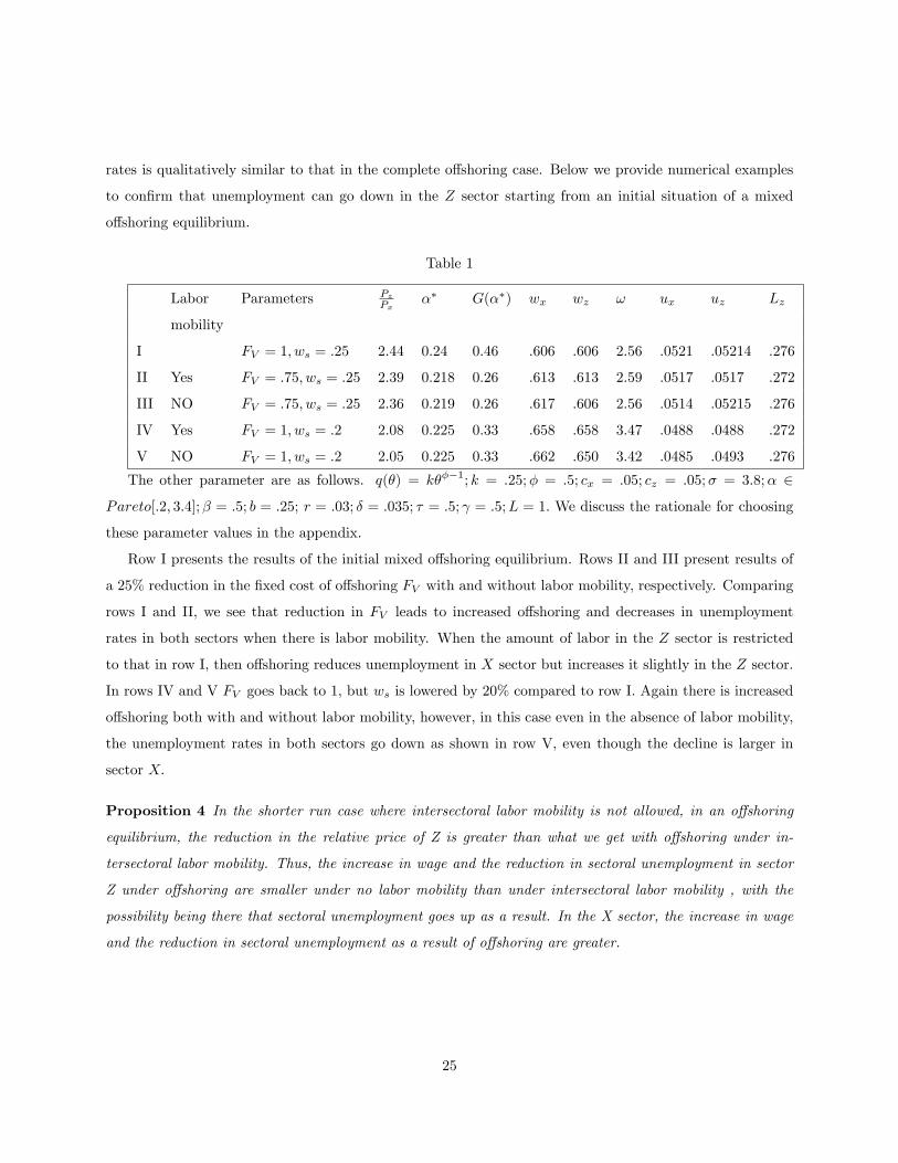
rates is qualitatively similar to that in the complete o¤shoring case. Below we provide numerical examples

to con�rm that unemployment can go down in the Z sector starting from an initial situation of a mixed

o¤shoring equilibrium.

Table 1

Labor Parameters PzPx

�� G(��) wx wz ! ux uz Lz

mobility

I FV = 1; ws = :25 2:44 0:24 0:46 :606 :606 2:56 :0521 :05214 :276

II Yes FV = :75; ws = :25 2:39 0:218 0:26 :613 :613 2:59 :0517 :0517 :272

III NO FV = :75; ws = :25 2:36 0:219 0:26 :617 :606 2:56 :0514 :05215 :276

IV Yes FV = 1; ws = :2 2:08 0:225 0:33 :658 :658 3:47 :0488 :0488 :272

V NO FV = 1; ws = :2 2:05 0:225 0:33 :662 :650 3:42 :0485 :0493 :276

The other parameter are as follows. q(�) = k���1; k = :25;� = :5; cx = :05; cz = :05;� = 3:8;� 2

Pareto[:2; 3:4];� = :5; b = :25; r = :03; � = :035; � = :5; = :5;L = 1: We discuss the rationale for choosing

these parameter values in the appendix.

Row I presents the results of the initial mixed o¤shoring equilibrium. Rows II and III present results of

a 25% reduction in the �xed cost of o¤shoring FV with and without labor mobility, respectively. Comparing

rows I and II, we see that reduction in FV leads to increased o¤shoring and decreases in unemployment

rates in both sectors when there is labor mobility. When the amount of labor in the Z sector is restricted

to that in row I, then o¤shoring reduces unemployment in X sector but increases it slightly in the Z sector.

In rows IV and V FV goes back to 1, but ws is lowered by 20% compared to row I. Again there is increased

o¤shoring both with and without labor mobility, however, in this case even in the absence of labor mobility,

the unemployment rates in both sectors go down as shown in row V, even though the decline is larger in

sector X:

Proposition 4 In the shorter run case where intersectoral labor mobility is not allowed, in an o¤shoring

equilibrium, the reduction in the relative price of Z is greater than what we get with o¤shoring under in-

tersectoral labor mobility. Thus, the increase in wage and the reduction in sectoral unemployment in sector

Z under o¤shoring are smaller under no labor mobility than under intersectoral labor mobility , with the

possibility being there that sectoral unemployment goes up as a result. In the X sector, the increase in wage

and the reduction in sectoral unemployment as a result of o¤shoring are greater.

25

4 An Extension: Free Entry

The extension we present here is allowing for free entry of �rms in the di¤erentiated inputs sector, so that

the mass of �rms operating in equilibrium is endogenously determined.11 We are back here to the case of

intersectoral labor mobility. As discussed in section 2, before entering, �rms incur a sunk cost equal to FE

in terms of the numeraire good. Then they observe their realization of productivity which they draw from

a distribution G(�); where � 2 [�; �]: The price of Z, Pz, can now be written as

Pz =M1

1��

24 �Z�

p(�)1��dG(�)

351

1��

(41)

where M is the mass of active �rms. Assuming �� to be the cuto¤ productivity above which �rms o¤shore,

the key equations determining the equilibrium in the case of endogenous entry are given as follows. The

pricing decision of di¤erentiated goods �rms is same as before. The equation determining cuto¤ productivity

�� is again given by (37) which can be written as

ZP�z (��)��1(CV � CD) = FV (42)

The only additional equation is the free entry condition in the di¤erentiated goods sector which can be

written as

ZP�z

24CV ��Z�

���1dG(�) + CD

�Z��

���1dG(�)

35 = FE + (1�G(��))FV (43)

The labor market clearing condition in the Z sector is modi�ed as follows.

(1� uz)Lz =MZP �z

��

(� � 1)

��� �wz +

(r + �)czq(�z)

��� 24��Z�

���1dG(�) + �!(��1)(1��)�Z��

���1dG(�)

35(44)

The product market clearing condition is still given by

Z

(1� ux)(L� Lz)= (Pz)

1 �1

(1� ) (45)

Equations (41)-(45) along with (60)-(66) in the appendix determine the following 12 endogenous variables

of interest:Px; Pz; wx; wz; �x;�z; ux; uz; Lz; Z; ��; and M:

11See Ziesemer (2005) for a completely autarkic, one sector model of unemployment under monopolistic competition.

26

Next, we show that the results obtained on the impact of o¤shoring on unemployment continue to hold

when the number of varieties is endogenously determined. Establishing this result analytically in the general

case is di¢ cult, therefore, we look at the case where cx = cz: In equilibrium, a potential entrant must be

indi¤erent between entering and not entering an industry. Let � be the expected annualized per period

pro�t of a potential new entrant in the di¤erentiated intermediate good sector when the economy is in the

steady state. This pro�t is net of both search and production costs, but gross of �xed costs and is given by

r times the expression on the left hand side of (43) Since we have cx = cz = ce; we have wx = wz = we,

�x = �z = �e; and ux = uz = ue; where the subscript e denotes �economywide�. Let R be the annualized

per period expected revenue of a potential new entrant. Given the markup equation we derived earlier, we

have � = R=�. Since C = Z X1�

(1� )1� , a constant share of total expenditure on C is indirectly on the Z

good and consequently on all the intermediate varieties, z(i) combined.

Total expenditure on the numeraire good C is the sum of the wage bill, total pro�ts net of �xed costs,

search costs. total �xed costs and export sales that pay for (therefore equal) the import of the o¤shored

production input. As explained earlier, incumbent �rms already in the steady state will earn rents relative to

a potential new entrant. Such rents will be earned by incumbent �rms in both sectors because each occupied

job has a value of ceq(�e)

. Let us denote total per-period rents of this type by �:12 We denote the total per

period expenditure on the o¤shored production input byM. Also, in our framework, when a �rm incurs a

sunk cost of entry, FE ; right in the beginning, it is equivalent to paying rFE every period. Recall that rFV

is the per period �xed cost of o¤shoring. With a total of M �rms producing the di¤erentiated intermediate

good z we have total revenue in the intermediate goods sector sector equal to total expenditure, Ez; on Z

MR = Ez = f(1� ue)weL+M [��(1�G(��))rFV �rFE ]+�+S+M [(1�G(��))rFV +rFE ]+Mg (46)

where S is the total search costs incurred by all �rms in the economy and is given in steady state by �ce(1�ue)Lq(�e)

.

In equilibrium with M endogenously determined, the free entry condition in (43) can be re-written as

� = (1�G(��))rFV + rFE (47)

using which and using the relation � = R=�; we have the equilibrium condition given by

� [(1�G(��))rFV + rFE ] =1

M f(1� ue)weL+ � + S +M [(1�G(��))rFV + rFE ] +Mg (48)

12The total annualized rents per period for the economy as a whole can be written as � = rce(1�ue)Lq(�e)

where as before the

subscript e stands for the common, economywide variable.

27

The above can be re-written as

[(1�G(��))rFV + rFE ] =

(� � )M f(1� ue)weL+ � + S +Mg (49)

which can be further re-written as

[(1�G(��))rFV + rFE ] =

(� � )M (we +(r + �)ceq(�e)

) (1� ue)L+ M

(� � )M (50)

Now, for a given ��, we and �e are increasing in M; while ue is decreasing in M: Therefore, (we +(r+�)ceq(�e)

) (1� ue)L on the r.h.s of the above equation is clearly increasing in M: In the case of autarky,

which equals the case where �� = � andM = 0; it is shown in the appendix that the proportional change

in (we +(r+�)ceq(�e)

) is less than the proportional change in M; and since the impact on ue is of second order,

(�� )M (we +(r+�)ceq(�e)

) (1� ue)L, which we from now on call '(M); would be decreasing in M in autarky.

[It is shown in the appendix that under the su¢ cient condition (� � 1) > (1� (1��)) , (we +

(r+�)ceq(�e)

) under

o¤shoring increases less than proportionally with M for any ��:] Therefore the r.h.s. of the last equation

which equals '(M) under autarky, is represented by a downward sloping EE curve in Figure 5.

When FV is small, for a given M; allowing for o¤shoring leads to complete o¤shoring, i.e., �� = � at

which point G(��) = 0: We now look at the various components of '(M) under complete o¤shoring and

under autarky. For a given M , we and �e are decreasing in ��; while ue is increasing in ��: Therefore,

(we +(r+�)ceq(�e)

) (1� ue)L is higher under o¤shoring than under autarky. On top of that now M>0, which

means exports are positive and add to the total demand for C and therefore to the expenditure on Z: Thus,

in Figure 5, the EE curve under complete o¤shoring, representing '(M) + M(�� )M ; lies completely above

the EE curve under no o¤shoring. The per-�rm total costs of entry and o¤shoring combined are greater

under complete o¤shoring than under no o¤shoring. If FV is relatively small, we clearly have equilibrium

M , given by the intersection of EE and the per �rm �xed cost curve, higher under complete o¤shoring

than under no o¤shoring. 13A higher M under o¤shoring implies that Pz is lower with endogenous M than

with M exogenously �xed at the autarky value; and hence unemployment is lower in a complete o¤shoring

equilibrium with endogenous M than with exogenous M:

Thus, with free entry, we have an increase in the total mass of �rms operating in the di¤erentiated

intermediate goods sector as a result of o¤shoring. This, clearly, is an additional channel through which

13This is true irrespective of the shape of the EE curve under complete o¤shoring, since it is completely above the downward

sloping EE curve under autarky. This means that the EE curve under o¤shoring cannot intersect the �xed cost curve to the

left of the equilibrium M under autarky (assuming �xed costs of o¤shoring are relatively small).

28

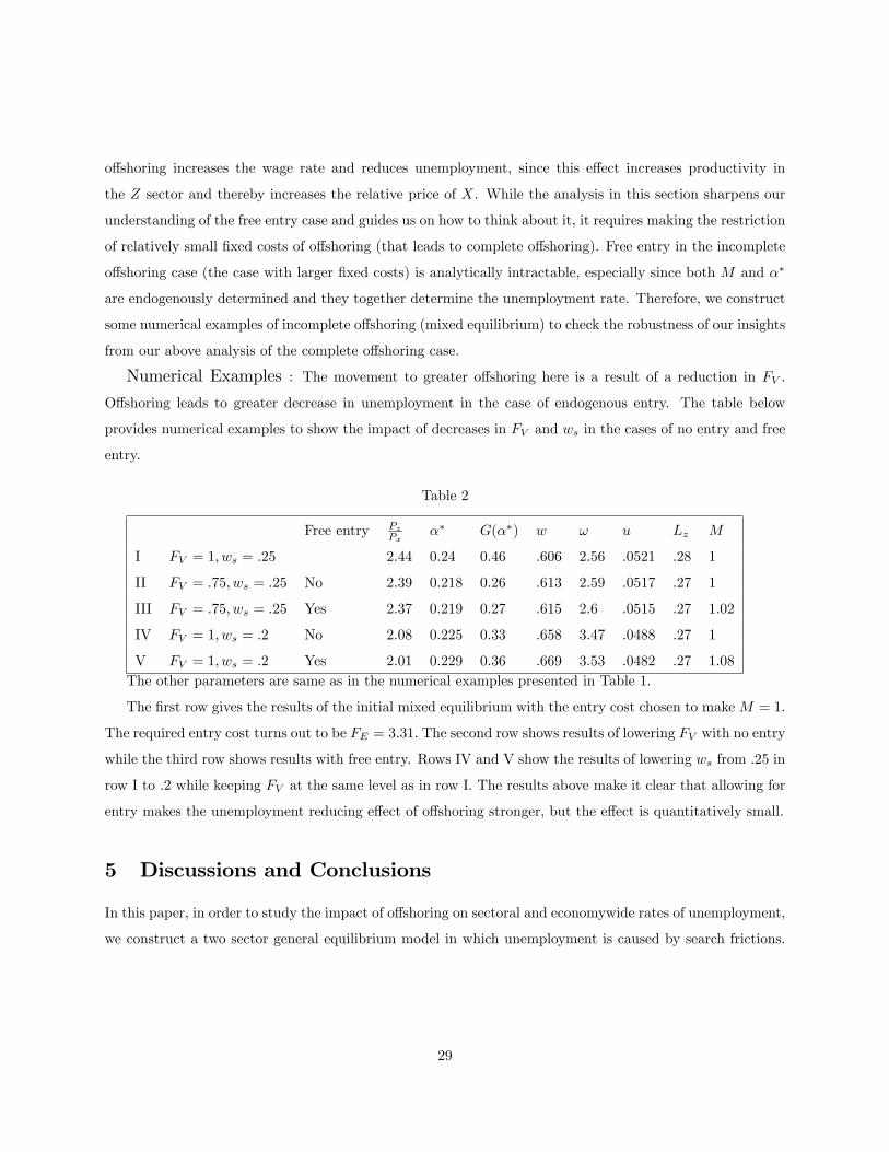
o¤shoring increases the wage rate and reduces unemployment, since this e¤ect increases productivity in

the Z sector and thereby increases the relative price of X. While the analysis in this section sharpens our

understanding of the free entry case and guides us on how to think about it, it requires making the restriction

of relatively small �xed costs of o¤shoring (that leads to complete o¤shoring). Free entry in the incomplete

o¤shoring case (the case with larger �xed costs) is analytically intractable, especially since both M and ��

are endogenously determined and they together determine the unemployment rate. Therefore, we construct

some numerical examples of incomplete o¤shoring (mixed equilibrium) to check the robustness of our insights

from our above analysis of the complete o¤shoring case.

Numerical Examples : The movement to greater o¤shoring here is a result of a reduction in FV :

O¤shoring leads to greater decrease in unemployment in the case of endogenous entry. The table below

provides numerical examples to show the impact of decreases in FV and ws in the cases of no entry and free

entry.

Table 2

Free entry PzPx

�� G(��) w ! u Lz M

I FV = 1; ws = :25 2:44 0:24 0:46 :606 2:56 :0521 :28 1

II FV = :75; ws = :25 No 2:39 0:218 0:26 :613 2:59 :0517 :27 1

III FV = :75; ws = :25 Yes 2:37 0:219 0:27 :615 2:6 :0515 :27 1:02

IV FV = 1; ws = :2 No 2:08 0:225 0:33 :658 3:47 :0488 :27 1

V FV = 1; ws = :2 Yes 2:01 0:229 0:36 :669 3:53 :0482 :27 1:08

The other parameters are same as in the numerical examples presented in Table 1.

The �rst row gives the results of the initial mixed equilibrium with the entry cost chosen to makeM = 1:

The required entry cost turns out to be FE = 3:31: The second row shows results of lowering FV with no entry

while the third row shows results with free entry. Rows IV and V show the results of lowering ws from .25 in

row I to .2 while keeping FV at the same level as in row I. The results above make it clear that allowing for

entry makes the unemployment reducing e¤ect of o¤shoring stronger, but the e¤ect is quantitatively small.

5 Discussions and Conclusions

In this paper, in order to study the impact of o¤shoring on sectoral and economywide rates of unemployment,

we construct a two sector general equilibrium model in which unemployment is caused by search frictions.

29

We �nd that, contrary to general perception, wage increases and sectoral unemployment decreases due to

o¤shoring. This result can be understood to arise from the productivity enhancing (cost reducing) e¤ect of

o¤shoring. This result is consistent with the recent empirical results of Amiti and Wei (2005a, b) for the

US and UK, where, when sectors are de�ned broadly enough, they �nd no evidence of a negative e¤ect of

o¤shoring on sectoral employment.

Even though both sectors have lower unemployment post-o¤shoring, whether the sector with the lower

unemployment or higher unemployment expands will also be a determinant of the overall unemployment

rate. If the search cost is identical in the two sectors, implying identical rates of unemployment, then the

economywide rate of unemployment declines unambiguously after o¤shoring. Alternatively, even if the search

cost is higher in the sector which experiences o¤shoring (implying a higher wage as well as higher rate of

unemployment in that sector), the economywide rate of unemployment decreases because workers move from

the higher unemployment sector to the lower unemployment sector. Interestingly, when the possibility of

o¤shoring is allowed for we �nd the existence of multiple equilibria, resulting in the indeterminacy of sectoral

and overall unemployment rates.

Next, the domestic employment of �rms that o¤shore may be higher than those of �rms that decide not

to o¤shore. This arises from the complementarity between headquarter services and production that can

be o¤shored, as well as from the business stealing e¤ect. These e¤ects can also increase a �rm�s domestic

employment after o¤shoring relative to its pre-o¤shoring level.

When we modify the model to disallow intersectoral labor mobility, the negative relative price e¤ect on

the sector in which �rms o¤shore some of their production activity becomes stronger. In such a case, it is

possible for this e¤ect to o¤set the positive productivity e¤ect, and result in a rise in unemployment in that

sector. In the other sector, o¤shoring has a much stronger unemployment reducing e¤ect in the absence of

intersectoral labor mobility than in the presence of it.

Finally, allowing for an endogenous number varieties in the o¤shoring sector provides an additional

indirect channel through which sectoral unemployment goes down.

Before ending the paper some remarks on some of our modeling assumptions are in order. Instead of

writing a two sector model, we could have written a one sector model to examine the impact of o¤shoring

on unemployment. We have veri�ed that the unemployment reducing e¤ect of o¤shoring is present even in

a one sector model with endogenous entry a la Melitz (2003), but we preferred a two sector model because

it provides additional insights about the intersectoral reallocation. We have modeled vacancy cost, c; in

terms of the numeraire good which seemed natural given the two sector structure of the model. One could

30

alternatively model the vacancy cost either in terms of labor or foregone output. In the former case, the

vacancy cost would be ciwi for sector i = X;Z; where wi is the sectoral wage. In the latter case, it would

be cipi: Our preliminary investigation suggests that the qualitative results would be unchanged.

The model in the paper can be extended along several dimensions. In our current paper we do not

explicitly model outsourcing, as is currently understood to be subject to contracting problems.14 If �rms

have the choice to outsource their production activities to a foreign supplier in an incomplete contract

framework, whether a �rm outsources or produces inputs domestically will depend on the tradeo¤ between

the domestic labor market frictions and contracting costs.

Another possible extension would be to endogenize the bargaining power of workers in the wage bargaining

process. In our current model, wages increase with o¤shoring, however, there is some evidence to suggest

that wages of workers have stagnated despite productivity gains coming from globalization and technological

progress. If we make workers�bargaining power a decreasing function of the number of �rms o¤shoring, it

would be possible to show a decrease in wages resulting from o¤shoring. This would be similar in spirit to

the Mitchell (1985) description of �norm shift�in wage determination. Since our focus in the present paper

is on unemployment e¤ects of o¤shoring, we do not pursue this extension in the present paper.

We can also extend the model to allow for workers with di¤erent skills and see whether o¤shoring a¤ects

them di¤erentially. We plan to pursue these extensions in a separate paper, as they seem to be beyond the

scope of the current one.

References

[1] Amiti, M. and Wei, S. (2005a). �Fear of service outsourcing,�Economic Policy, April, 307-347.

[2] Amiti, M. and Wei, S. (2005b). �Service O¤shoring, Productivity, and Employment: Evidence from the

United States,�IMF Working Paper WP/05/238.

[3] Antras, P. (2003). �Firms, Contracts, and Trade Structure,�Quarterly Journal of Economics 118 (4),

1374-1418.

[4] Antras, P. and Helpman, E. (2004). �Global Sourcing,�Journal of Political Economy 112(3), 552-580.

14See the very brief literature review in the introduction. Also, see Mitra and Ranjan (2005) for an explcit modeling of

incomplete contracts, in the context of external economies of o¤shoring (but not in the context of unemployment).

31

[5] Bardhan, A. and Kroll, C. (2003). �The New Wave of Outsourcing,�Research Report, Fisher Center

for Real Estate and Urban Economics, University of California, Berkeley, Fall.

[6] Bernard, A.; Eaton, J.; Jensen, J. B.and Kortum, S., 2003, �Plants and Productivity in International

Trade�American Economic Review 93(4), 1268-1290.

[7] Bhagwati, J.; Panagariya, A. and Srinivasan, T.N. (2004). �The Muddles over Outsourcing,� Journal

of Economic Perspectives 18(4), 93-114.

[8] Blanchard, O. and Diamond. P.(1989). �The Beveridge curve�, Brookings Papers on Economic Activity,

vol. 1 , pp.1-76.

[9] Blinder, A. (2006). �O¤shoring: The Next Industrial Revolution?" Foreign A¤airs, March/April 2006,

pp. 113-128.

[10] Brecher, R.(1974a).�Optimal commercial policy for a minimum-wage economy,�Journal of International

Economics, vol. 4, (no.2), pp. 139-49.

[11] Brecher, R.(1974b), �Minimum wage rates and the pure theory of international trade,�Quarterly Journal

of Economics, vol.88, (no.1), pp. 98-116.

[12] Brecher, R. (1992). �An e¢ ciency-wage model with explicit monitoring: Unemployment and welfare in

an open economy,�Journal of International Economics, vol.32(1-2), pp. 179-91.

[13] Brecher, R., Choudhri, E. (1994). �Pareto gains from trade reconsidered: Compensating for jobs lost,�

Journal of International-Economics; vol.36(3-4), pp. 223-38.

[14] Copeland, B.(1989). �E¢ ciency wages in a Ricardian model of international trade,�Journal of Inter-

national Economics, vol. 27, pp. 221-244.

[15] Davidson, C. and Matusz, S. (2004). International Trade and Labor Markets, WE Upjohn Institute of

Employment Research, Kalamazoo, Michigan.

[16] Davidson, C.; Matusz, S. and Shevchenko, A. (2006). �Outsourcing Peter to Pay Paul: High Skill

Expectations and Low-Skill Wages and Imperfect Labor Markets,�mimeo, Department of Economics,

Michigan State University.

32

[17] Davis, D.(1998a). �Does European unemployment prop up American wages? National labour markets

and global trade,�American Economic Review, vol. 88, pp.478-94.

[18] Davis, D.(1998b). �Technology, unemployment, and relative wages in a global economy,� European

Economic Review, vol. 42, pp.1613-33.

[19] Drezner, D. (2004). �The outsourcing bogeyman,�Foreign A¤airs, May/June.

[20] Ethier, W. (1982). �National and International Returns to Scale in the Modern Theory of International

Trade,�American Economic Review 73, 389-405.

[21] Feenstra, R.C. and Hanson, G. H. (2005). �Ownership and Control in Outsourcing to China: Estimating

the Property Rights Theory of the Firm,�Quarterly Journal of Economics 120(2): 729-762.

[22] Grossman, G. and Helpman, E. (2002). �Integration versus Outsourcing in Industry Equilibrium,�

Quarterly Journal of Economics 117(468), 85-120.

[23] Grossman, G. and Helpman, E. (2003). �Outsourcing versus FDI in Industry Equilibrium,�Journal of

the European Economic Association 1(2), 317-327..

[24] Grossman, G. and Helpman, E. (2005). �Outsourcing in a Global Economy,�Review of Economic Studies

72(1), 135-159.

[25] Grossman, G. and Rossi-Hansberg, E. (2006). �Trading Tasks: A Simple Theory of O¤shoring,�mimeo,

Princeton University.

[26] Hoon, H. T. (2001) �Adjustment of wages and equilibrium unemployment in a Ricardian global econ-

omy,�Journal of International Economics, vol. 54, pp. 193-209.

[27] Hosios, A. (1990). �Factor market search and the structure of simple general equilibrium models,�

Journal of Political Economy, vol.98, (no.2), pp. 325-355.

[28] Karabay, B. and McLaren, J. (2006). �Trade, Outsourcing and the Invisible Handshake,�mimeo, De-

partment of Economics, University of Virginia.

[29] Matusz, S. (1986).�Implicit contracts, unemployment and international trade,�Economic Journal, vol.

96, (382), pp. 307-22.

33

[30] Matusz, S. (1994). �International trade policy in a model of unemployment and wage di¤erential,�

Canadian Journal of Economics, vol. 27, (no.4), pp. 939-949.

[31] McKinsey & Company (2005). The Emerging Global Labor Market, June.

[32] Melitz. M. 2003, �The Impact of trade on intra-industry reallocations and aggregate industry produc-

tivity,�Econometrica 71, 1695-1725.

[33] Mitchell, D.(1985). �Shifting norms in wage determination,�Brookings Papers on Economic Activity,

Vol. 2, pp. 575-99.

[34] Mitra, D. and Ranjan, P. (2005). �Temporary Shocks and O¤shoring: The Role of External Economies

and Firm Heterogeneity,�mimeo, Syracuse University and University of California - Irvine.

[35] Moore, M. and Ranjan, P. (2005). �Globalization vs skill biased technical change: Implications for

unemployment and wage inequality,�Economic Journal, April.

[36] Pissarides, C. (2000). Equilibrium Unemployment Theory, 2nd ed.,Cambridge, MA: MIT Press.

[37] Rodriguez-Clare, A. (2006). �O¤shoring in a Ricardian World,� mimeo, Department of Economics,

Pennsylvania State University.

[38] Sener, F. (2001) �Schumpeterian unemployment, trade and wages�, Journal of International Economics,

vol. 54 , pp. 119-148.

[39] Ziesemer, T. (2005) �Monopolistic Competition and Search Unemployment, Metroeconomica,�Vol. 56,

No. 3, pp. 334-359.

34

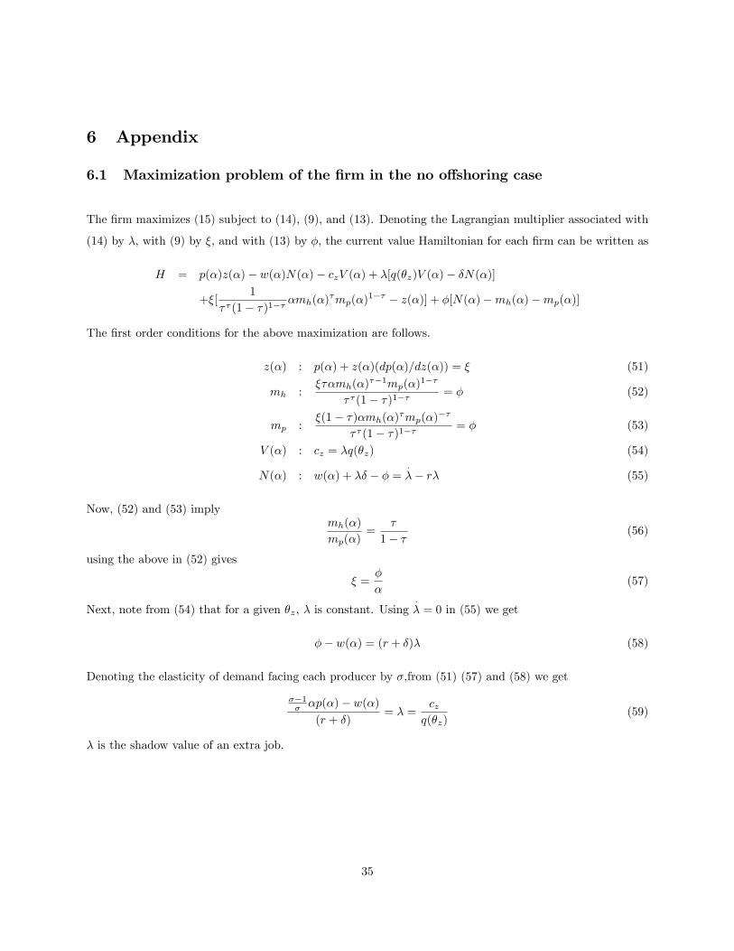
6 Appendix

6.1 Maximization problem of the �rm in the no o¤shoring case

The �rm maximizes (15) subject to (14), (9), and (13). Denoting the Lagrangian multiplier associated with

(14) by �, with (9) by �, and with (13) by �; the current value Hamiltonian for each �rm can be written as

H = p(�)z(�)� w(�)N(�)� czV (�) + �[q(�z)V (�)� �N(�)]

+�[1

� � (1� �)1�� �mh(�)�mp(�)

1�� � z(�)] + �[N(�)�mh(�)�mp(�)]

The �rst order conditions for the above maximization are follows.

z(�) : p(�) + z(�)(dp(�)=dz(�)) = � (51)

mh :���mh(�)

��1mp(�)1��

� � (1� �)1�� = � (52)

mp :�(1� �)�mh(�)

�mp(�)��

� � (1� �)1�� = � (53)

V (�) : cz = �q(�z) (54)

N(�) : w(�) + �� � � =:

�� r� (55)

Now, (52) and (53) implymh(�)

mp(�)=

�

1� � (56)

using the above in (52) gives

� =�

�(57)

Next, note from (54) that for a given �z, � is constant. Using:

� = 0 in (55) we get

�� w(�) = (r + �)� (58)

Denoting the elasticity of demand facing each producer by �;from (51) (57) and (58) we get

��1� �p(�)� w(�)

(r + �)= � =

czq(�z)

(59)

� is the shadow value of an extra job.

35

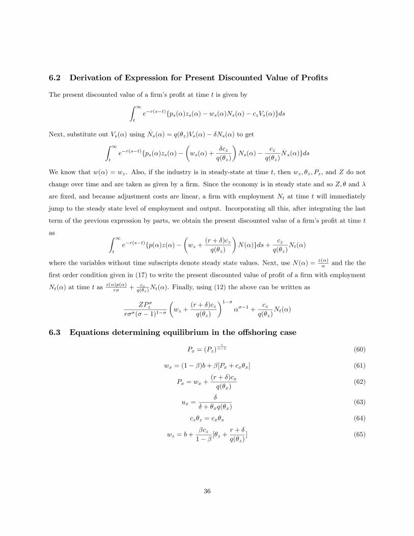
6.2 Derivation of Expression for Present Discounted Value of Pro�ts

The present discounted value of a �rm�s pro�t at time t is given byZ 1

t

e�r(s�t)fps(�)zs(�)� ws(�)Ns(�)� czVs(�)gds

Next, substitute out Vs(�) using:

Ns(�) = q(�z)Vs(�)� �Ns(�) to getZ 1

t

e�r(s�t)fps(�)zs(�)��ws(�) +

�czq(�z)

�Ns(�)�

czq(�z)

:

Ns(�)gds

We know that w(�) = wz. Also, if the industry is in steady-state at time t; then wz; �z; Pz; and Z do not

change over time and are taken as given by a �rm. Since the economy is in steady state and so Z; � and �

are �xed, and because adjustment costs are linear, a �rm with employment Nt at time t will immediately

jump to the steady state level of employment and output. Incorporating all this, after integrating the last

term of the previous expression by parts, we obtain the present discounted value of a �rm�s pro�t at time t

as Z 1

t

e�r(s�t)fp(�)z(�)��wz +

(r + �)czq(�z)

�N(�)gds+ cz

q(�z)Nt(�)

where the variables without time subscripts denote steady state values. Next, use N(�) = z(�)� and the the

�rst order condition given in (17) to write the present discounted value of pro�t of a �rm with employment

Nt(�) at time t asz(�)p(�)

r� + czq(�z)

Nt(�). Finally, using (12) the above can be written as

ZP�zr��(� � 1)1��

�wz +

(r + �)czq(�z)

�1�����1 +

czq(�z)

Nt(�)

6.3 Equations determining equilibrium in the o¤shoring case

Px = (Pz)

�1 (60)

wx = (1� �)b+ �[Px + cx�x] (61)

Px = wx +(r + �)cxq(�x)

(62)

ux =�

� + �xq(�x)(63)

cz�z = cx�x (64)

wz = b+�cz1� � [�z +

r + �

q(�z)] (65)

36

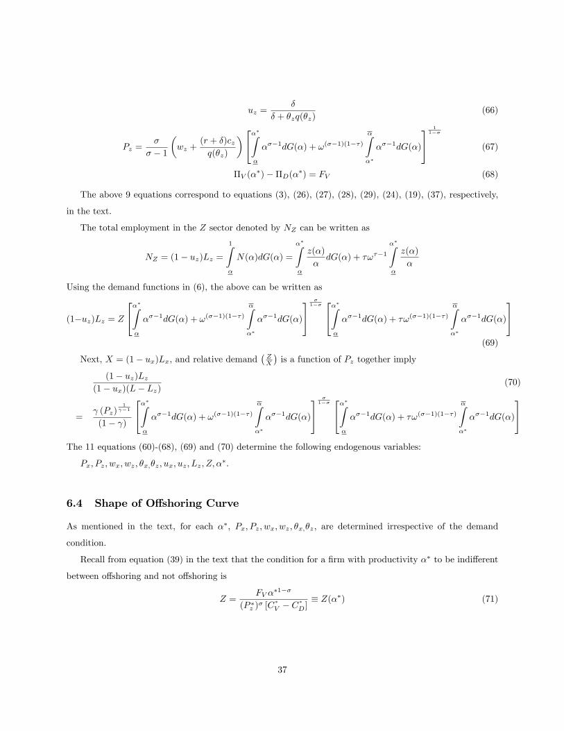
uz =�

� + �zq(�z)(66)

Pz =�

� � 1

�wz +

(r + �)czq(�z)

�24��Z�

���1dG(�) + !(��1)(1��)�Z��

���1dG(�)

351

1��

(67)

�V (��)��D(��) = FV (68)

The above 9 equations correspond to equations (3), (26), (27), (28), (29), (24), (19), (37), respectively,

in the text.

The total employment in the Z sector denoted by NZ can be written as

NZ = (1� uz)Lz =1Z�

N(�)dG(�) =

��Z�

z(�)

�dG(�) + �!��1

��Z�

z(�)

�

Using the demand functions in (6), the above can be written as

(1�uz)Lz = Z

24��Z�

���1dG(�) + !(��1)(1��)�Z��

���1dG(�)

35�

1�� 24��Z�

���1dG(�) + �!(��1)(1��)�Z��

���1dG(�)

35(69)

Next, X = (1� ux)Lx; and relative demand�ZX

�is a function of Pz together imply

(1� uz)Lz(1� ux)(L� Lz)

(70)

= (Pz)

1 �1

(1� )

24��Z�

���1dG(�) + !(��1)(1��)�Z��

���1dG(�)

35�

1�� 24��Z�

���1dG(�) + �!(��1)(1��)�Z��

���1dG(�)

35The 11 equations (60)-(68), (69) and (70) determine the following endogenous variables:

Px; Pz; wx; wz; �x;�z; ux; uz; Lz; Z; ��:

6.4 Shape of O¤shoring Curve

As mentioned in the text, for each ��; Px; Pz; wx; wz; �x;�z; are determined irrespective of the demand

condition.

Recall from equation (39) in the text that the condition for a �rm with productivity �� to be indi¤erent

between o¤shoring and not o¤shoring is

Z =FV �

�1��

(P �z )� [C

�V � C

�D]� Z(��) (71)

37

Our aim is to �nd out what happens to the minimum required Z when �� is lowered. As mentioned in the

text, a decrease in �� implies increases in Px; wx; wz; �x;�z and a decrease in Pz: Therefore, a su¢ cient, but

by no means necessary, condition for Z 0(��) < 0 is that CV � CD is increasing in ��: Note that

CV � CD �

�wz +

(r+�)czq(�z)

�1�� �!(��1)(1��) � 1

�r��(� � 1)1��

Therefore,

d log(CV � CD)d��

= (1� �)d log

�wz +

(r+�)czq(�z)

�d��

+d log

�!(��1)(1��) � 1

�d��

which can be re-written as

d log(CV � CD)d��

=d log

�wz +

(r+�)czq(�z)

�(� � 1)

d��

"1� �!(��1)(1��)�!(��1)(1��) � 1

�#

Since wz and �z are decreasing in ��;d log(wz+ (r+�)cz

q(�z))

d�� < 0; and hence, d log(CV �CD)d�� > 0 i¤

! >

�1

�

� 1(��1)(1��)

(72)

It can be seen that the term on the rhs of (72) is decreasing in � and � : Therefore, (72) is easily satis�ed

for high � and � : Also, since wz and �z are decreasing in ��; a su¢ cient condition for Z 0(��) < 0 is

!NO >�1�

� 1(��1)(1��) : (Recall that !� > !NO 8�� � �):

Since we want to plot the o¤shoring curve in ( ZX ;PzPx) space, we want to establish that Z 0(��) < 0 implies

Z(��)X(��) is also decreasing in �

�: De�ne (��) � Z(��)X(��) : Using (69) write the relationship between output and

employment in the Z sector as

Z(��) = A(��)(1� uz(��))Lz(��) (73)

where

A(��) =

24��Z�

���1dG(�) + !(��1)(1��)�Z��

���1dG(�)

35�

��1 24��Z�

���1dG(�) + �!(��1)(1��)�Z��

���1dG(�)

35�1(74)

Z 0(��) < 0 implies d lnA(��)

d�� + d ln(1�uz(��))d�� + d lnLz(�

�)d�� < 0: Since d ln(1�uz(�

�))d�� is, relative to the other terms,

a second-order e¤ect, we take d ln(1�uz(��))d�� � 0; and so e¤ectively, Z 0(��) < 0 implies �d lnA(��)

d�� > d lnLZd�� :

Next, (��) = A(��)Lz(��)

L�Lz(��) if cx = cz:Therefore, we have

38

d ln (��)

d��=d lnA(��)

d��+d lnLz(�

�)

d��+

Lz(��)

L� Lz(��)d lnLz(�

�)

d��=d lnA(��)

d��+1

lx

d lnLz(��)

d��(75)

where lx = (L�Lz(��))=L: Therefore, d ln (��)

d�� < 0 when1

lx

d lnLz(��)

d�� < �d lnA(��)d�� :We discuss two possible

cases.

Case I: d lnLz(��)

d�� < 0: In this case d lnLz(��)

d�� >1

lx

d lnLz(��)

d�� : Therefore, Z 0(��) < 0 implies1

lx

d lnLz(��)

d�� <

�d lnA(��)d�� :

Case II: d lnLz(��)

d�� > 0: In this case Z 0(��) < 0 implies �d lnA(��)d�� > 0: So, for d ln (��)

d�� < 0 we need

lx >�d lnLz(�

�)d��

�=��d lnA(��)

d��

�: [Note that d lnLz(�

�)d�� � d lnZ(��)

d�� � d lnA(��)d�� < �d lnA(��)

d�� here and so

0 <�d lnLz(�

�)d��

�=��d lnA(��)

d��

�< 1, as is 0 < lx < 1:]:

We �nd no indication of the violation of the inequality restriction,1

lx

d lnLz(��)

d�� < �d lnA(��)d�� from the

several numerical examples, constructed with reasonable parameter values, that show that whenever Z 0(��) <

0; we have 0(��) < 0 as well.

6.5 Sectoral reallocation of labor after o¤shoring

Claim: cx = cz implies that the labor force in the Z sector is smaller in an o¤shoring equilibrium than under

a no-o¤shoring equilibrium.

Proof:cx = cz implies ux = uz and

Px = wz +(r + �)czq(�z)

(76)

The relative demand for Z equal to relative supply in an o¤shoring equilibrium given in (70)

above can be re-written as

Lz(L� Lz)

= (1� ux) (Pz)

1 �1

(1� uz)(1� )[A(��)]

�1 (77)

where A(��) is de�ned in (74). Let LOz denote the size of the labor force in the Z sector in an

o¤shoring equilibrium and LNOz the size of the labor force in the Z sector in the no-o¤shoring

equilibrium. The expression for LNOz is obtained by setting �� = � in the above expression. �� =

� will capture the complete o¤shoring case. From equation (77) above we see that LOz < LNOz

requires

[A(��)]�1 e� < � Pz

PNOz

� 11�

(78)

39

Next, using (76) the expression for Pz given in (67) above can be written as

Pz =�

� � 1Px

24��Z�

���1dG(�) + !(��1)(1��)�Z��

���1dG(�)

351

1��

Also, from (60) Px = (Pz)

�1 : Therefore,

(Pz)1

1� =�

� � 1

24��Z�

���1dG(�) + !(��1)(1��)�Z��

���1dG(�)

351

1��

(79)

Similarly, �PNOz

� 11� =

��

� � 1e��1�

(80)

Using (79) and (80) on the rhs of (78) and cancelling terms we get

� < 1

Therefore, LOz < LNOz for any � < 1: QED

6.6 Free Entry Case: Condition for '(M) to be decreasing in M

Write the expression for Pz as follows.

Pz =�

� � 1M1

1��

�wz +

(r + �)czq(�z)

�24��Z�

���1dG(�) + !(��1)(1��)�Z��

���1dG(�)

351

1��

Note that, for cx = cz case Px = wz +(r+�)czq(�z)

: Substituting this in the above expression and noting that

Pz = (Px) �1 ; we can write the above as

(Px)�1 =

�

� � 1M1

1��

24��Z�

���1dG(�) +P(��1)(1��)x

w(��1)(1��)s

�Z��

���1dG(�)

351

1��

The above implies that2666666641�

(1� �)!(��1)(1��)�Z��

���1dG(�)

24��Z�

���1dG(�) + !(��1)(1��)

�Z��

���1dG(�)

35

377777775d logPxd logM

=

� � 1

40

In the case of autarky, �� � �; therefore, d logPxd logM =

��1 < 1: In the complete o¤shoring case, �� = �;

therefore, the above impliesd logPxd logM

=

(� � 1)(1� (1� �))

Thus, d logPxd logM < 1 as long as (��1)(1� (1��)) < 1 or (� � 1) >

(1� (1��)) : Note from the above that for any

�� 2 (�; �) the condition (� � 1) > (1� (1��)) is su¢ cient for

d logPxd logM < 1:

6.7 Parameters for numerical examples

� = 3:8 and � 2 Pareto[:2; 3:4] are taken from Bernard, Eaton, Jensen and Kortum (2003). � = :035

corresponds to the monthly average job destruction rate in the United States. The time preference parameter,

r = :03; is in the range of values commonly used in Macro literature. m = kv�u1�� is the standard matching

function used in the literature and our choice of � = :5 is in the range of the estimate of this matching

parameter in Blanchard and Diamond (1989) where it ranges from .43 to .75. k = :25 was chosen to get

reasonable values of unemployment rates. The Nash bargaining parameter � = :5 is the most commonly

used in the literature. In the absence of any clear guidance for other parameters we tried many di¤erent

values and found the results to be robust to their alternative values. We report the results obtained using

some speci�c values.

41

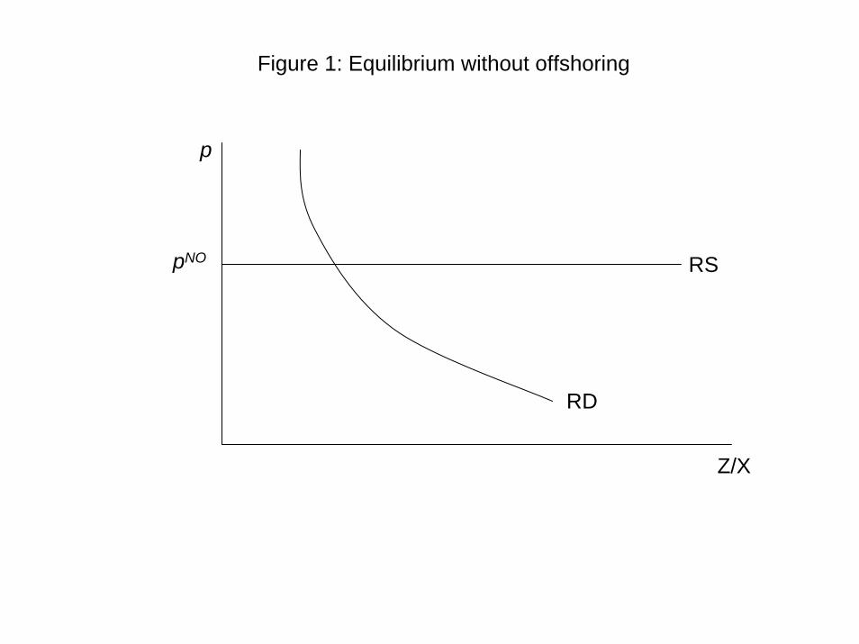
Figure 1: Equilibrium without offshoring

pNO

Z/X

RD

RS

p

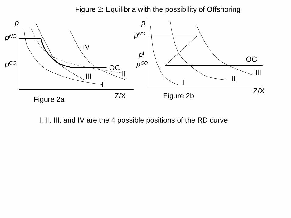
pNO

Z/X

OC

Figure 2a

Figure 2: Equilibria with the possibility of Offshoring

I

IV

III

pNO

Z/X

OC

II

Figure 2b

pI

pCO

IIII

II

p p

pCO

I, II, III, and IV are the 4 possible positions of the RD curve

pNO

Z/XFigure 3a: Decrease in FV

OC

pNO

Z/XFigure 3b: Decrease in ws

OCpCO

Figure 3: Comparative Statics

OC’

OC’

RDRD

A

B

A

B

Z/X

OC’

Figure 3c: Increase in b

OC

RD

B

A

p

p p

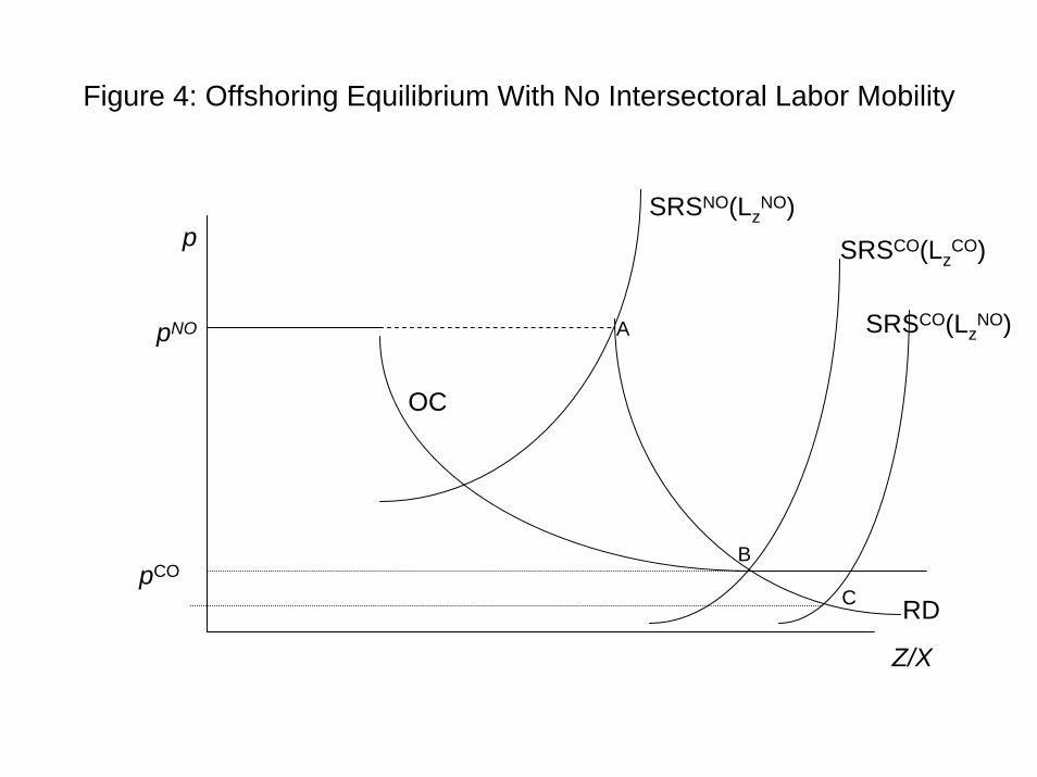
Figure 4: Offshoring Equilibrium With No Intersectoral Labor Mobility

pNO

pCO

Z/X

OC

RD

SRSCO(LzCO)

SRSNO(LzNO)

SRSCO(LzNO)A

B

C

p

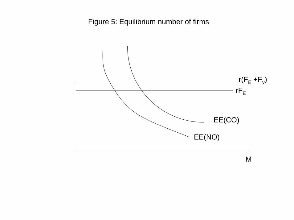
Figure 5: Equilibrium number of firms

M

EE(NO)

rFE

EE(CO)

r(FE +Fv)