offshore hydromechanics by j.m.j. journee w.w. massie
TRANSCRIPT
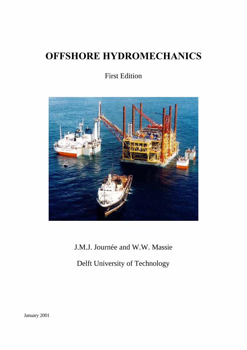
OFFSHORE HYDROMECHANICS
First Edition
J.M.J. Journée and W.W. Massie
Delft University of Technology
January 2001

0-2
Contents
1 INTRODUCTION 1-11.1 De…nition of Motions . . . . . . . . . . . . . . . . . . . . . . . . . . . . . . 1-21.2 Problems of Interest . . . . . . . . . . . . . . . . . . . . . . . . . . . . . . 1-3
1.2.1 Suction Dredgers . . . . . . . . . . . . . . . . . . . . . . . . . . . . 1-31.2.2 Pipe Laying Vessels . . . . . . . . . . . . . . . . . . . . . . . . . . . 1-51.2.3 Drilling Vessels . . . . . . . . . . . . . . . . . . . . . . . . . . . . . 1-71.2.4 Oil Production and Storage Units . . . . . . . . . . . . . . . . . . . 1-81.2.5 Support Vessels . . . . . . . . . . . . . . . . . . . . . . . . . . . . . 1-161.2.6 Transportation Vessels . . . . . . . . . . . . . . . . . . . . . . . . . 1-19
2 HYDROSTATICS 2-12.1 Introduction . . . . . . . . . . . . . . . . . . . . . . . . . . . . . . . . . . . 2-12.2 Static Loads . . . . . . . . . . . . . . . . . . . . . . . . . . . . . . . . . . . 2-2
2.2.1 Hydrostatic Pressure . . . . . . . . . . . . . . . . . . . . . . . . . . 2-22.2.2 Archimedes Law and Buoyancy . . . . . . . . . . . . . . . . . . . . 2-22.2.3 Internal Static Loads . . . . . . . . . . . . . . . . . . . . . . . . . . 2-22.2.4 Drill String Buckling . . . . . . . . . . . . . . . . . . . . . . . . . . 2-52.2.5 Pipeline on Sea Bed . . . . . . . . . . . . . . . . . . . . . . . . . . 2-6
2.3 Static Floating Stability . . . . . . . . . . . . . . . . . . . . . . . . . . . . 2-62.3.1 De…nitions . . . . . . . . . . . . . . . . . . . . . . . . . . . . . . . . 2-72.3.2 Equilibrium . . . . . . . . . . . . . . . . . . . . . . . . . . . . . . . 2-82.3.3 Shifting Masses and Volumes . . . . . . . . . . . . . . . . . . . . . 2-102.3.4 Righting Moments . . . . . . . . . . . . . . . . . . . . . . . . . . . 2-122.3.5 Metacenter . . . . . . . . . . . . . . . . . . . . . . . . . . . . . . . 2-132.3.6 Scribanti Formula . . . . . . . . . . . . . . . . . . . . . . . . . . . . 2-152.3.7 Stability Curve . . . . . . . . . . . . . . . . . . . . . . . . . . . . . 2-172.3.8 Eccentric Loading . . . . . . . . . . . . . . . . . . . . . . . . . . . . 2-212.3.9 Inclining Experiment . . . . . . . . . . . . . . . . . . . . . . . . . . 2-242.3.10 Free Surface Correction . . . . . . . . . . . . . . . . . . . . . . . . . 2-25
3 CONSTANT POTENTIAL FLOW PHENOMENA 3-13.1 Introduction . . . . . . . . . . . . . . . . . . . . . . . . . . . . . . . . . . . 3-13.2 Basis Flow Properties . . . . . . . . . . . . . . . . . . . . . . . . . . . . . . 3-1
3.2.1 Continuity Condition . . . . . . . . . . . . . . . . . . . . . . . . . . 3-13.2.2 Deformation and Rotation . . . . . . . . . . . . . . . . . . . . . . . 3-4
3.3 Potential Flow Concepts . . . . . . . . . . . . . . . . . . . . . . . . . . . . 3-63.3.1 Potentials . . . . . . . . . . . . . . . . . . . . . . . . . . . . . . . . 3-6
0-3
0-4 CONTENTS
3.3.2 Euler Equations . . . . . . . . . . . . . . . . . . . . . . . . . . . . . 3-83.3.3 Bernoulli Equation . . . . . . . . . . . . . . . . . . . . . . . . . . . 3-93.3.4 2-D Streams . . . . . . . . . . . . . . . . . . . . . . . . . . . . . . . 3-103.3.5 Properties . . . . . . . . . . . . . . . . . . . . . . . . . . . . . . . . 3-12
3.4 Potential Flow Elements . . . . . . . . . . . . . . . . . . . . . . . . . . . . 3-133.4.1 Uniform Flow Elements . . . . . . . . . . . . . . . . . . . . . . . . 3-133.4.2 Source and Sink Elements . . . . . . . . . . . . . . . . . . . . . . . 3-143.4.3 Circulation or Vortex Elements . . . . . . . . . . . . . . . . . . . . 3-15
3.5 Superposition of Basic Elements . . . . . . . . . . . . . . . . . . . . . . . . 3-163.5.1 Methodology . . . . . . . . . . . . . . . . . . . . . . . . . . . . . . 3-163.5.2 Sink (or Source) in Uniform Flow . . . . . . . . . . . . . . . . . . . 3-183.5.3 Separated Source and Sink . . . . . . . . . . . . . . . . . . . . . . . 3-183.5.4 Source and Sink in Uniform Flow . . . . . . . . . . . . . . . . . . . 3-203.5.5 Rankine Ship Forms . . . . . . . . . . . . . . . . . . . . . . . . . . 3-203.5.6 Doublet or Dipole . . . . . . . . . . . . . . . . . . . . . . . . . . . . 3-203.5.7 Doublet in Uniform Flow . . . . . . . . . . . . . . . . . . . . . . . . 3-213.5.8 Pipeline Near The Sea Bed . . . . . . . . . . . . . . . . . . . . . . . 3-23
3.6 Single Cylinder in a Uniform Flow . . . . . . . . . . . . . . . . . . . . . . . 3-253.6.1 Flow . . . . . . . . . . . . . . . . . . . . . . . . . . . . . . . . . . . 3-253.6.2 Pressures . . . . . . . . . . . . . . . . . . . . . . . . . . . . . . . . 3-263.6.3 Resulting Forces . . . . . . . . . . . . . . . . . . . . . . . . . . . . 3-27
4 CONSTANT REAL FLOW PHENOMENA 4-14.1 Introduction . . . . . . . . . . . . . . . . . . . . . . . . . . . . . . . . . . . 4-14.2 Basic Viscous Flow Concepts . . . . . . . . . . . . . . . . . . . . . . . . . 4-1
4.2.1 Boundary Layer and Viscosity . . . . . . . . . . . . . . . . . . . . . 4-14.2.2 Turbulence . . . . . . . . . . . . . . . . . . . . . . . . . . . . . . . 4-24.2.3 Newton’s Friction Force Description . . . . . . . . . . . . . . . . . . 4-3
4.3 Dimensionless Ratios and Scaling Laws . . . . . . . . . . . . . . . . . . . . 4-44.3.1 Physical Model Relationships . . . . . . . . . . . . . . . . . . . . . 4-44.3.2 Reynolds Scaling . . . . . . . . . . . . . . . . . . . . . . . . . . . . 4-64.3.3 Froude Scaling . . . . . . . . . . . . . . . . . . . . . . . . . . . . . 4-74.3.4 Numerical Example . . . . . . . . . . . . . . . . . . . . . . . . . . . 4-7
4.4 Cylinder Flow Regimes . . . . . . . . . . . . . . . . . . . . . . . . . . . . . 4-84.5 Drag and Lift . . . . . . . . . . . . . . . . . . . . . . . . . . . . . . . . . . 4-8
4.5.1 Drag Force and Drag Coe¢cient . . . . . . . . . . . . . . . . . . . . 4-8
4.5.2 Lift Force and Strouhal Number . . . . . . . . . . . . . . . . . . . . 4-124.6 Vortex Induced Oscillations . . . . . . . . . . . . . . . . . . . . . . . . . . 4-15
4.6.1 Crosswise Oscillations . . . . . . . . . . . . . . . . . . . . . . . . . 4-164.6.2 In-Line Oscillations . . . . . . . . . . . . . . . . . . . . . . . . . . . 4-17
4.7 Ship Still Water Resistance . . . . . . . . . . . . . . . . . . . . . . . . . . . 4-174.7.1 Frictional Resistance . . . . . . . . . . . . . . . . . . . . . . . . . . 4-194.7.2 Residual Resistance . . . . . . . . . . . . . . . . . . . . . . . . . . . 4-204.7.3 Extrapolation of Resistance Tests . . . . . . . . . . . . . . . . . . . 4-224.7.4 Resistance Prediction Methods . . . . . . . . . . . . . . . . . . . . 4-23
4.8 Wind Loads . . . . . . . . . . . . . . . . . . . . . . . . . . . . . . . . . . . 4-234.8.1 Wind Loads on Moored Ships . . . . . . . . . . . . . . . . . . . . . 4-25
CONTENTS 0-5
4.8.2 Wind Loads on Other Moored Structures . . . . . . . . . . . . . . . 4-264.8.3 Wind Loads on Sailing Ships . . . . . . . . . . . . . . . . . . . . . . 4-27
4.9 Current Loads . . . . . . . . . . . . . . . . . . . . . . . . . . . . . . . . . . 4-294.9.1 Current Loads on Moored Tankers . . . . . . . . . . . . . . . . . . 4-304.9.2 Current Loads on Other Moored Structures . . . . . . . . . . . . . 4-314.9.3 Current Loads on Sailing Ships . . . . . . . . . . . . . . . . . . . . 4-32
4.10 Thrust and Propulsion . . . . . . . . . . . . . . . . . . . . . . . . . . . . . 4-324.10.1 Propulsors . . . . . . . . . . . . . . . . . . . . . . . . . . . . . . . . 4-334.10.2 Propeller Geometry . . . . . . . . . . . . . . . . . . . . . . . . . . . 4-354.10.3 Propeller Mechanics . . . . . . . . . . . . . . . . . . . . . . . . . . 4-404.10.4 Ship Propulsion . . . . . . . . . . . . . . . . . . . . . . . . . . . . . 4-444.10.5 Propulsion versus Resistance . . . . . . . . . . . . . . . . . . . . . . 4-474.10.6 Lift and Flettner Rotors . . . . . . . . . . . . . . . . . . . . . . . . 4-48
5 OCEAN SURFACE WAVES 5-15.1 Introduction . . . . . . . . . . . . . . . . . . . . . . . . . . . . . . . . . . . 5-15.2 Regular Waves . . . . . . . . . . . . . . . . . . . . . . . . . . . . . . . . . 5-2
5.2.1 Potential Theory . . . . . . . . . . . . . . . . . . . . . . . . . . . . 5-45.2.2 Phase Velocity . . . . . . . . . . . . . . . . . . . . . . . . . . . . . 5-115.2.3 Water Particle Kinematics . . . . . . . . . . . . . . . . . . . . . . . 5-125.2.4 Pressure . . . . . . . . . . . . . . . . . . . . . . . . . . . . . . . . . 5-165.2.5 Energy . . . . . . . . . . . . . . . . . . . . . . . . . . . . . . . . . . 5-175.2.6 Relationships Summary . . . . . . . . . . . . . . . . . . . . . . . . 5-225.2.7 Shoaling Water . . . . . . . . . . . . . . . . . . . . . . . . . . . . . 5-225.2.8 Wave Re‡ection and Di¤raction . . . . . . . . . . . . . . . . . . . . 5-255.2.9 Splash Zone . . . . . . . . . . . . . . . . . . . . . . . . . . . . . . . 5-26
5.3 Irregular Waves . . . . . . . . . . . . . . . . . . . . . . . . . . . . . . . . . 5-295.3.1 Wave Superposition . . . . . . . . . . . . . . . . . . . . . . . . . . . 5-295.3.2 Wave Measurements . . . . . . . . . . . . . . . . . . . . . . . . . . 5-295.3.3 Simple Statistical Analysis . . . . . . . . . . . . . . . . . . . . . . . 5-315.3.4 More Complete Record Analysis . . . . . . . . . . . . . . . . . . . . 5-34
5.4 Wave Energy Spectra . . . . . . . . . . . . . . . . . . . . . . . . . . . . . . 5-375.4.1 Basic Principles . . . . . . . . . . . . . . . . . . . . . . . . . . . . . 5-385.4.2 Energy Density Spectrum . . . . . . . . . . . . . . . . . . . . . . . 5-385.4.3 Standard Wave Spectra . . . . . . . . . . . . . . . . . . . . . . . . . 5-435.4.4 Transformation to Time Series . . . . . . . . . . . . . . . . . . . . . 5-46
5.5 Wave Prediction and Climatology . . . . . . . . . . . . . . . . . . . . . . . 5-485.5.1 Single Storm . . . . . . . . . . . . . . . . . . . . . . . . . . . . . . . 5-515.5.2 Long Term . . . . . . . . . . . . . . . . . . . . . . . . . . . . . . . . 5-555.5.3 Statistics . . . . . . . . . . . . . . . . . . . . . . . . . . . . . . . . . 5-57
6 RIGID BODY DYNAMICS 6-16.1 Introduction . . . . . . . . . . . . . . . . . . . . . . . . . . . . . . . . . . . 6-16.2 Ship De…nitions . . . . . . . . . . . . . . . . . . . . . . . . . . . . . . . . . 6-1
6.2.1 Axis Conventions . . . . . . . . . . . . . . . . . . . . . . . . . . . . 6-26.2.2 Frequency of Encounter . . . . . . . . . . . . . . . . . . . . . . . . 6-36.2.3 Motions of and about CoG . . . . . . . . . . . . . . . . . . . . . . . 6-46.2.4 Displacement, Velocity and Acceleration . . . . . . . . . . . . . . . 6-4
0-6 CONTENTS
6.2.5 Motions Superposition . . . . . . . . . . . . . . . . . . . . . . . . . 6-56.3 Single Linear Mass-Spring System . . . . . . . . . . . . . . . . . . . . . . . 6-7
6.3.1 Kinetics . . . . . . . . . . . . . . . . . . . . . . . . . . . . . . . . . 6-86.3.2 Hydromechanical Loads . . . . . . . . . . . . . . . . . . . . . . . . 6-96.3.3 Wave Loads . . . . . . . . . . . . . . . . . . . . . . . . . . . . . . . 6-196.3.4 Equation of Motion . . . . . . . . . . . . . . . . . . . . . . . . . . . 6-216.3.5 Response in Regular Waves . . . . . . . . . . . . . . . . . . . . . . 6-226.3.6 Response in Irregular Waves . . . . . . . . . . . . . . . . . . . . . . 6-246.3.7 Spectrum Axis Transformation . . . . . . . . . . . . . . . . . . . . 6-26
6.4 Second Order Wave Drift Forces . . . . . . . . . . . . . . . . . . . . . . . . 6-276.4.1 Mean Wave Loads on a Wall . . . . . . . . . . . . . . . . . . . . . . 6-276.4.2 Mean Wave Drift Forces . . . . . . . . . . . . . . . . . . . . . . . . 6-326.4.3 Low-Frequency Wave Drift Forces . . . . . . . . . . . . . . . . . . . 6-336.4.4 Additional Responses . . . . . . . . . . . . . . . . . . . . . . . . . . 6-35
6.5 Time Domain Approach . . . . . . . . . . . . . . . . . . . . . . . . . . . . 6-366.5.1 Impulse Response Functions . . . . . . . . . . . . . . . . . . . . . . 6-366.5.2 Direct Time Domain Simulation . . . . . . . . . . . . . . . . . . . . 6-42
7 POTENTIAL COEFFICIENTS 7-17.1 Introduction . . . . . . . . . . . . . . . . . . . . . . . . . . . . . . . . . . . 7-17.2 Principles . . . . . . . . . . . . . . . . . . . . . . . . . . . . . . . . . . . . 7-1
7.2.1 Requirements . . . . . . . . . . . . . . . . . . . . . . . . . . . . . . 7-27.2.2 Forces and Moments . . . . . . . . . . . . . . . . . . . . . . . . . . 7-47.2.3 Hydrodynamic Loads . . . . . . . . . . . . . . . . . . . . . . . . . . 7-57.2.4 Wave and Di¤raction Loads . . . . . . . . . . . . . . . . . . . . . . 7-97.2.5 Hydrostatic Loads . . . . . . . . . . . . . . . . . . . . . . . . . . . 7-11
7.3 2-D Potential Theory . . . . . . . . . . . . . . . . . . . . . . . . . . . . . . 7-127.3.1 Theory of Ursell . . . . . . . . . . . . . . . . . . . . . . . . . . . . . 7-137.3.2 Conformal Mapping . . . . . . . . . . . . . . . . . . . . . . . . . . 7-207.3.3 Theory of Tasai . . . . . . . . . . . . . . . . . . . . . . . . . . . . . 7-267.3.4 Theory of Frank . . . . . . . . . . . . . . . . . . . . . . . . . . . . . 7-307.3.5 Comparative Results . . . . . . . . . . . . . . . . . . . . . . . . . . 7-36
7.4 3-D Potential Theory . . . . . . . . . . . . . . . . . . . . . . . . . . . . . . 7-367.4.1 Di¤raction Theory . . . . . . . . . . . . . . . . . . . . . . . . . . . 7-377.4.2 Solving Potentials . . . . . . . . . . . . . . . . . . . . . . . . . . . . 7-417.4.3 Numerical Aspects . . . . . . . . . . . . . . . . . . . . . . . . . . . 7-43
7.5 Experimental Determination . . . . . . . . . . . . . . . . . . . . . . . . . . 7-467.5.1 Free Decay Tests . . . . . . . . . . . . . . . . . . . . . . . . . . . . 7-467.5.2 Forced Oscillation Tests . . . . . . . . . . . . . . . . . . . . . . . . 7-48
7.6 Viscous Damping . . . . . . . . . . . . . . . . . . . . . . . . . . . . . . . . 7-517.6.1 Viscous Surge Damping . . . . . . . . . . . . . . . . . . . . . . . . 7-517.6.2 Viscous Roll Damping . . . . . . . . . . . . . . . . . . . . . . . . . 7-51
8 FLOATING STRUCTURES IN WAVES 8-18.1 Introduction . . . . . . . . . . . . . . . . . . . . . . . . . . . . . . . . . . . 8-18.2 Kinetics . . . . . . . . . . . . . . . . . . . . . . . . . . . . . . . . . . . . . 8-18.3 Coupled Equations of Motion . . . . . . . . . . . . . . . . . . . . . . . . . 8-3
8.3.1 General De…nition . . . . . . . . . . . . . . . . . . . . . . . . . . . 8-3
CONTENTS 0-7
8.3.2 Motion Symmetry of Ships . . . . . . . . . . . . . . . . . . . . . . . 8-48.3.3 2-D Strip Theory . . . . . . . . . . . . . . . . . . . . . . . . . . . . 8-58.3.4 3-D Panel Method . . . . . . . . . . . . . . . . . . . . . . . . . . . 8-17
8.4 Motions in Regular Waves . . . . . . . . . . . . . . . . . . . . . . . . . . . 8-198.4.1 Frequency Characteristics . . . . . . . . . . . . . . . . . . . . . . . 8-198.4.2 Harmonic Motions . . . . . . . . . . . . . . . . . . . . . . . . . . . 8-228.4.3 Dynamic Swell-Up . . . . . . . . . . . . . . . . . . . . . . . . . . . 8-25
8.5 Motions in Irregular Waves . . . . . . . . . . . . . . . . . . . . . . . . . . . 8-278.5.1 Spectrum Transformations . . . . . . . . . . . . . . . . . . . . . . . 8-278.5.2 Response Spectra . . . . . . . . . . . . . . . . . . . . . . . . . . . . 8-308.5.3 First Order Motions . . . . . . . . . . . . . . . . . . . . . . . . . . 8-328.5.4 Probability of Exceeding . . . . . . . . . . . . . . . . . . . . . . . . 8-34
8.6 Liquids in Tanks . . . . . . . . . . . . . . . . . . . . . . . . . . . . . . . . 8-358.6.1 Anti-Roll Tanks . . . . . . . . . . . . . . . . . . . . . . . . . . . . . 8-368.6.2 Tank Loads . . . . . . . . . . . . . . . . . . . . . . . . . . . . . . . 8-38
8.7 Internal Loads . . . . . . . . . . . . . . . . . . . . . . . . . . . . . . . . . . 8-428.7.1 Basic Approach . . . . . . . . . . . . . . . . . . . . . . . . . . . . . 8-448.7.2 Static Equilibrium . . . . . . . . . . . . . . . . . . . . . . . . . . . 8-458.7.3 Quasi-Static Equilibrium . . . . . . . . . . . . . . . . . . . . . . . . 8-478.7.4 Dynamic Equilibrium . . . . . . . . . . . . . . . . . . . . . . . . . . 8-498.7.5 Internal Loads Spectra . . . . . . . . . . . . . . . . . . . . . . . . . 8-528.7.6 Fatigue Assessments . . . . . . . . . . . . . . . . . . . . . . . . . . 8-52
8.8 Added Resistance in Waves . . . . . . . . . . . . . . . . . . . . . . . . . . 8-548.8.1 Radiated Energy Method . . . . . . . . . . . . . . . . . . . . . . . . 8-548.8.2 Integrated Pressure Method . . . . . . . . . . . . . . . . . . . . . . 8-568.8.3 Non-dimensional Presentation . . . . . . . . . . . . . . . . . . . . . 8-588.8.4 Added Resistance in Irregular Waves . . . . . . . . . . . . . . . . . 8-58
9 NON-LINEAR BEHAVIOR 9-19.1 Introduction . . . . . . . . . . . . . . . . . . . . . . . . . . . . . . . . . . . 9-19.2 Some Typical Phenomena . . . . . . . . . . . . . . . . . . . . . . . . . . . 9-1
9.2.1 Bow-Hawser Moored Vessel in Wind and Current . . . . . . . . . . 9-19.2.2 Large Concrete Structure under Tow . . . . . . . . . . . . . . . . . 9-29.2.3 Horizontal Motions of Moored Tankers in Waves . . . . . . . . . . . 9-49.2.4 Motions and Mooring Forces of Semi-Submersibles . . . . . . . . . . 9-69.2.5 Vertical Motions of Ships in Long Waves . . . . . . . . . . . . . . . 9-89.2.6 Behavior of a Jetty-Moored Tanker . . . . . . . . . . . . . . . . . . 9-10
9.3 Wave Drift Forces and Moments . . . . . . . . . . . . . . . . . . . . . . . . 9-119.3.1 Second Order Wave Forces . . . . . . . . . . . . . . . . . . . . . . . 9-159.3.2 Second Order Wave Moments . . . . . . . . . . . . . . . . . . . . . 9-289.3.3 Quadratic Transfer Functions . . . . . . . . . . . . . . . . . . . . . 9-289.3.4 Computed Results of Wave Drift Forces . . . . . . . . . . . . . . . 9-349.3.5 Low Frequency Motions . . . . . . . . . . . . . . . . . . . . . . . . 9-389.3.6 Simple Frequency Domain Method . . . . . . . . . . . . . . . . . . 9-43
9.4 Remarks . . . . . . . . . . . . . . . . . . . . . . . . . . . . . . . . . . . . . 9-46
0-8 CONTENTS
10 STATION KEEPING 10-110.1 Introduction . . . . . . . . . . . . . . . . . . . . . . . . . . . . . . . . . . . 10-110.2 Mooring Systems . . . . . . . . . . . . . . . . . . . . . . . . . . . . . . . . 10-1
10.2.1 De…nitions . . . . . . . . . . . . . . . . . . . . . . . . . . . . . . . . 10-210.2.2 Static Catenary Line . . . . . . . . . . . . . . . . . . . . . . . . . . 10-410.2.3 Dynamic E¤ects . . . . . . . . . . . . . . . . . . . . . . . . . . . . . 10-810.2.4 Experimental Results . . . . . . . . . . . . . . . . . . . . . . . . . . 10-1210.2.5 Suspension Point Loads . . . . . . . . . . . . . . . . . . . . . . . . 10-12
10.3 Thrusters . . . . . . . . . . . . . . . . . . . . . . . . . . . . . . . . . . . . 10-1310.3.1 Characteristics . . . . . . . . . . . . . . . . . . . . . . . . . . . . . 10-1310.3.2 Loss of E¢ciency . . . . . . . . . . . . . . . . . . . . . . . . . . . . 10-14
10.4 Dynamic Positioning . . . . . . . . . . . . . . . . . . . . . . . . . . . . . . 10-2010.4.1 Control Systems . . . . . . . . . . . . . . . . . . . . . . . . . . . . . 10-2010.4.2 Mathematical Model . . . . . . . . . . . . . . . . . . . . . . . . . . 10-2210.4.3 Wind Feed-Forward . . . . . . . . . . . . . . . . . . . . . . . . . . . 10-2410.4.4 Gain Constants Estimate . . . . . . . . . . . . . . . . . . . . . . . . 10-2510.4.5 Motion Reference Filtering . . . . . . . . . . . . . . . . . . . . . . . 10-2610.4.6 Role of Model Tests . . . . . . . . . . . . . . . . . . . . . . . . . . . 10-27
11 OPERABILITY 11-111.1 Statistics . . . . . . . . . . . . . . . . . . . . . . . . . . . . . . . . . . . . . 11-1
11.1.1 Short Term Predictions . . . . . . . . . . . . . . . . . . . . . . . . . 11-111.1.2 Long Term Predictions . . . . . . . . . . . . . . . . . . . . . . . . . 11-211.1.3 Extreme Values . . . . . . . . . . . . . . . . . . . . . . . . . . . . . 11-2
11.2 Operating Limits of Ships . . . . . . . . . . . . . . . . . . . . . . . . . . . 11-911.2.1 Personnel Safety . . . . . . . . . . . . . . . . . . . . . . . . . . . . 11-911.2.2 Shipping Water . . . . . . . . . . . . . . . . . . . . . . . . . . . . . 11-1011.2.3 Slamming . . . . . . . . . . . . . . . . . . . . . . . . . . . . . . . . 11-1211.2.4 Sustained Sea Speed . . . . . . . . . . . . . . . . . . . . . . . . . . 11-16
11.3 Dredger Limitations . . . . . . . . . . . . . . . . . . . . . . . . . . . . . . 11-2711.3.1 Dredger Wave Limitations . . . . . . . . . . . . . . . . . . . . . . . 11-2711.3.2 Dredger Current Limitations . . . . . . . . . . . . . . . . . . . . . . 11-27
12 WAVE FORCES ON SLENDER CYLINDERS 12-112.1 Introduction . . . . . . . . . . . . . . . . . . . . . . . . . . . . . . . . . . . 12-112.2 Basic Assumptions and De…nitions . . . . . . . . . . . . . . . . . . . . . . 12-112.3 Force Components in Oscillating Flows . . . . . . . . . . . . . . . . . . . . 12-2
12.3.1 Inertia Forces . . . . . . . . . . . . . . . . . . . . . . . . . . . . . . 12-312.3.2 Drag Forces . . . . . . . . . . . . . . . . . . . . . . . . . . . . . . . 12-7
12.4 Morison Equation . . . . . . . . . . . . . . . . . . . . . . . . . . . . . . . . 12-812.4.1 Experimental Discovery Path . . . . . . . . . . . . . . . . . . . . . 12-812.4.2 Morison Equation Coe¢cient Determination . . . . . . . . . . . . . 12-912.4.3 Typical Coe¢cient Values . . . . . . . . . . . . . . . . . . . . . . . 12-1712.4.4 Inertia or Drag Dominance . . . . . . . . . . . . . . . . . . . . . . . 12-20
12.5 Forces on A Fixed Cylinder in Various Flows . . . . . . . . . . . . . . . . . 12-2212.5.1 Current Alone . . . . . . . . . . . . . . . . . . . . . . . . . . . . . . 12-2212.5.2 Waves Alone . . . . . . . . . . . . . . . . . . . . . . . . . . . . . . . 12-2312.5.3 Currents plus Waves . . . . . . . . . . . . . . . . . . . . . . . . . . 12-24
CONTENTS 0-9
12.6 Forces on An Oscillating Cylinder in Various Flows . . . . . . . . . . . . . 12-2512.6.1 Still Water . . . . . . . . . . . . . . . . . . . . . . . . . . . . . . . . 12-2512.6.2 Current Alone . . . . . . . . . . . . . . . . . . . . . . . . . . . . . . 12-2512.6.3 Waves Alone . . . . . . . . . . . . . . . . . . . . . . . . . . . . . . . 12-2512.6.4 Currents Plus Waves . . . . . . . . . . . . . . . . . . . . . . . . . . 12-28
12.7 Force Integration over A Structure . . . . . . . . . . . . . . . . . . . . . . 12-28
13 SURVIVAL LOADS ON TOWER STRUCTURES 13-113.1 Introduction . . . . . . . . . . . . . . . . . . . . . . . . . . . . . . . . . . . 13-1
13.1.1 Method Requirements . . . . . . . . . . . . . . . . . . . . . . . . . 13-313.1.2 Analysis Steps . . . . . . . . . . . . . . . . . . . . . . . . . . . . . . 13-3
13.2 Environmental Conditions to Choose . . . . . . . . . . . . . . . . . . . . . 13-313.3 Ambient Flow Schematizations . . . . . . . . . . . . . . . . . . . . . . . . 13-613.4 Structure Schematization . . . . . . . . . . . . . . . . . . . . . . . . . . . . 13-813.5 Force Computation . . . . . . . . . . . . . . . . . . . . . . . . . . . . . . . 13-1013.6 Force and Moment Integration . . . . . . . . . . . . . . . . . . . . . . . . . 13-11
13.6.1 Horizontal Force Integration . . . . . . . . . . . . . . . . . . . . . . 13-1113.6.2 Overturning Moment Integration . . . . . . . . . . . . . . . . . . . 13-11
13.7 Comparative Example . . . . . . . . . . . . . . . . . . . . . . . . . . . . . 13-12
14 SEA BED BOUNDARY EFFECTS 14-114.1 Introduction . . . . . . . . . . . . . . . . . . . . . . . . . . . . . . . . . . . 14-114.2 Boundary Layer under Currents and Waves . . . . . . . . . . . . . . . . . . 14-2
14.2.1 Bed Shear Stress With Currents Alone . . . . . . . . . . . . . . . . 14-314.2.2 Boundary Layer Under Waves . . . . . . . . . . . . . . . . . . . . . 14-514.2.3 Shear Stress Under Waves Alone . . . . . . . . . . . . . . . . . . . 14-514.2.4 Shear Stress Under Waves Plus Currents . . . . . . . . . . . . . . . 14-6
14.3 Bed Material Stability . . . . . . . . . . . . . . . . . . . . . . . . . . . . . 14-814.3.1 Force Balance . . . . . . . . . . . . . . . . . . . . . . . . . . . . . . 14-914.3.2 Shields Shear Stress Approach . . . . . . . . . . . . . . . . . . . . . 14-1014.3.3 Link to Sediment Transport . . . . . . . . . . . . . . . . . . . . . . 14-11
14.4 Sediment Transport Process . . . . . . . . . . . . . . . . . . . . . . . . . . 14-1114.4.1 Time and Distance Scales . . . . . . . . . . . . . . . . . . . . . . . 14-1114.4.2 Mechanisms . . . . . . . . . . . . . . . . . . . . . . . . . . . . . . . 14-1214.4.3 Relative Importance of Bed versus Suspended Load . . . . . . . . . 14-14
14.5 Sea Bed Changes . . . . . . . . . . . . . . . . . . . . . . . . . . . . . . . . 14-1514.5.1 Sediment Transport Not Su¢cient for Bed Changes . . . . . . . . . 14-1514.5.2 Bed Change Time Scale . . . . . . . . . . . . . . . . . . . . . . . . 14-16
14.6 Laboratory Modeling . . . . . . . . . . . . . . . . . . . . . . . . . . . . . . 14-1614.6.1 Theoretical Background and Scaling . . . . . . . . . . . . . . . . . 14-1614.6.2 A Modeling Experience . . . . . . . . . . . . . . . . . . . . . . . . . 14-18
14.7 Vertical Pile in Current . . . . . . . . . . . . . . . . . . . . . . . . . . . . . 14-1914.7.1 Two Dimensional Approach . . . . . . . . . . . . . . . . . . . . . . 14-1914.7.2 Three Dimensional Flow . . . . . . . . . . . . . . . . . . . . . . . . 14-1914.7.3 Drag Force Changes . . . . . . . . . . . . . . . . . . . . . . . . . . 14-22
14.8 Small Objects on The Sea Bed . . . . . . . . . . . . . . . . . . . . . . . . . 14-2414.8.1 Burial Mechanisms . . . . . . . . . . . . . . . . . . . . . . . . . . . 14-24
14.9 Pipelines . . . . . . . . . . . . . . . . . . . . . . . . . . . . . . . . . . . . . 14-26
0-10 CONTENTS
14.9.1 Flow and Forces . . . . . . . . . . . . . . . . . . . . . . . . . . . . . 14-2714.9.2 Cover Layers . . . . . . . . . . . . . . . . . . . . . . . . . . . . . . 14-30
A TABLES A-1A.1 Greek Symbols . . . . . . . . . . . . . . . . . . . . . . . . . . . . . . . . . A-1A.2 Water Constants . . . . . . . . . . . . . . . . . . . . . . . . . . . . . . . . A-2
B MODELING AND MODEL SCALES B-1B.1 Introduction and Motivations . . . . . . . . . . . . . . . . . . . . . . . . . B-1B.2 Model Types . . . . . . . . . . . . . . . . . . . . . . . . . . . . . . . . . . B-1B.3 Basic Phenomena and Scales . . . . . . . . . . . . . . . . . . . . . . . . . . B-3B.4 Derived Scales . . . . . . . . . . . . . . . . . . . . . . . . . . . . . . . . . . B-3B.5 Forces to Model . . . . . . . . . . . . . . . . . . . . . . . . . . . . . . . . . B-4B.6 Force Scaling . . . . . . . . . . . . . . . . . . . . . . . . . . . . . . . . . . B-5B.7 Dimensionless Ratios . . . . . . . . . . . . . . . . . . . . . . . . . . . . . . B-6B.8 Practical Compromises . . . . . . . . . . . . . . . . . . . . . . . . . . . . . B-8B.9 Conclusion . . . . . . . . . . . . . . . . . . . . . . . . . . . . . . . . . . . . B-10
C FOURIER SERIES APPROXIMATIONS C-1C.1 Basic Form . . . . . . . . . . . . . . . . . . . . . . . . . . . . . . . . . . . C-1C.2 Derived Form . . . . . . . . . . . . . . . . . . . . . . . . . . . . . . . . . . C-2C.3 Limits . . . . . . . . . . . . . . . . . . . . . . . . . . . . . . . . . . . . . . C-2C.4 Application Example . . . . . . . . . . . . . . . . . . . . . . . . . . . . . . C-3
CONTENTS 0-11
PREFACEThis text book is an attempt to provide a comprehensive treatment of hydromechanicsfor o¤shore engineers. This text has originally been written for students participating inthe Interfaculty O¤shore Technology curriculum at the Delft University of Technology.O¤shore Hydromechanics forms the link in this curriculum between earlier courses onOceanography and (regular as well as irregular) Ocean Waves on the one hand, and thedesign of Fixed, Floating and Subsea Structures on the other.Topics have been selected for inclusion based upon their applicability in modern o¤shoreengineering practice. The treatment of these selected topics includes both the backgroundtheory and its applications to realistic problems.The book encompasses applied hydrodynamics for the seas outside the breaker zone. Popu-larly, one can say that this book uses information on wind, waves and currents to determineexternal forces on all sorts of structures in the sea as well as the stability and motions of‡oating structures and even of the sea bed itself. Only a short period of re‡ection isneeded to conclude that this covers a lot of ocean and quite some topics as well! Indeedthe following application examples illustrate this.The notation used in this book is kept as standard as possible, but is explained as itis introduced in each chapter. In some cases the authors have chosen to use notationcommonly found in the relevant literature - even if it is in con‡ict with a more universalstandard or even with other parts of this text. This is done to prepare students betterto read the literature if they wish to pursue such maters more deeply. In some othercases, the more or less standard notation and conventions have been adhered to in spiteof more common practice. An example of this latter disparity can be found in chapter14; conventions and notation used there do not always agree with those of the coastalengineers.One will discover that many equations are used in the explanation of the theories presentedin this book. In order to make reader reference easier, important theoretical results andequations have been enclosed in boxes. A few appendices have been used to collect relevantreference information which can be useful for reference or in more than one chapter.
Modular Structure of the BookAn O¤shore Hydromechanics course based upon this text can be built up from four re-lated modules. Each module has its own content and objectives; each module representsapproximately the same amount of (student) work. Within certain limitations, readers canchoose to work only with one or more from these modules relevant to their own needs:
1. Hydrostatics, Constant Flow Phenomena and Surface Waves.Upon completion of this segment students will understand hydrostatics as it relatesto all forms of structures. Compressive buckling of free-hanging drill strings is ex-plained Constant potential as well as real ‡ows and the forces which they can exerton structures complete this module along with a review of wave theory and wavestatistics.
0J.M.J. Journée and W.W. Massie, ”OFFSHORE HYDROMECHANICS”, First Edition, January 2001,Delft University of Technology. For updates see web site: http://www.shipmotions.nl.
0-12 CONTENTS
Module 1 covers chapter 1, a small part of chapter 2 and chapters 3, 4 and 5. Itprovides basic knowledge for all the succeeding modules; every course should includethis module. Module 1 can be succeeded by modules 2 and/or 4.
2. Static Floating Stability, Principles of Loads and Motions and Potential Theories.Upon completion of this segment students will become experienced with stabilitycomputations for all sorts of ‡oating structures - including those with partially …lledwater ballast tanks, etc. They will understand the basic application of linear potentialtheory to ships and other ‡oating structures for the computation of external andinternal forces, as well as the principle of motions of bodies in waves.Module 2 covers chapters 2, 6, and 7. It should be scheduled directly after module 1and prepares the student for the further development of this topic in module 3.
3. Loads and Motions in Waves, Nonlinear Hydrodynamics, Station Keeping and Op-erability.Students completing this segment will be able to predict the behavior of ‡oating orsailing bodies more completely. They will be familiar with …rst order ship motions inwaves, as well as nonlinear phenomena such as mean and second order drift forces.Applications such as station keeping and the determination of o¤shore workabilitywill be familiar.Module 3 covers the chapters 8, 9, 10 and 11. It should follow module 2 in thescheduling.
4. Slender Cylinder Hydrodynamics and Sea Bed Morphology.Students completing this segment will be familiar with the Morison equation andits extensions as well as with methods to determine its coe¢cients and approximatemethods for predicting the survival loads on an o¤shore tower structure. The com-putation of forces on pipelines as well as the morphological interaction between thesea bed and pipelines and other small objects will be familiar too.Module 4 covers chapters 12, 13 and 14. It can be scheduled directly after module 1and parallel with modules 2 and 3, if desired.
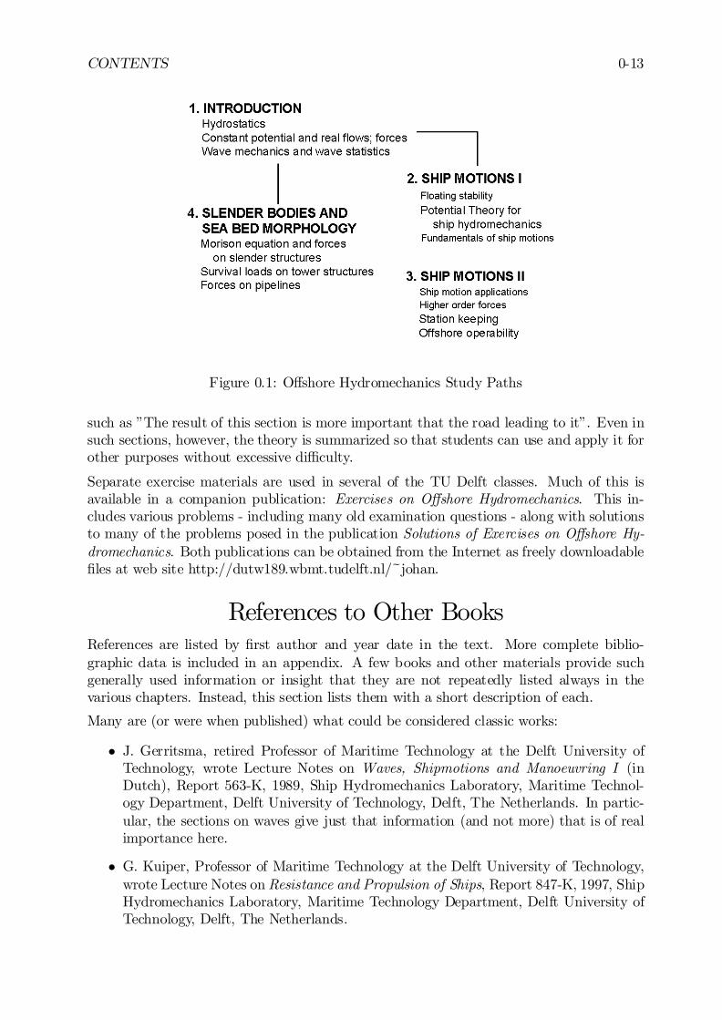
These modules are listed below and shown in the …gure 0.1 as well.Each of the following module combinations can be appropriate for speci…c groups of stu-dents; each path can be completed via a contiguous series of classes if desired.
Modules Objective Suited for
1,2,3,4CompleteCourse
O¤shore Technologyand any others optionally
1,2,3CompleteShip Motions
Marine TechnologyDredging Technology
1,2LimitedShip Motions
Dredging Technology, Civiland Mechanical Engineering
1,4Slender StructureLoads
Civil and MechanicalEngineering
The overall objective of this text is to use theory where necessary to solve practical o¤shoreengineering problems. Some sections which become rather mathematical contain a warning
CONTENTS 0-13
Figure 0.1: O¤shore Hydromechanics Study Paths
such as ”The result of this section is more important that the road leading to it”. Even insuch sections, however, the theory is summarized so that students can use and apply it forother purposes without excessive di¢culty.
Separate exercise materials are used in several of the TU Delft classes. Much of this isavailable in a companion publication: Exercises on O¤shore Hydromechanics. This in-cludes various problems - including many old examination questions - along with solutionsto many of the problems posed in the publication Solutions of Exercises on O¤shore Hy-dromechanics. Both publications can be obtained from the Internet as freely downloadable…les at web site http://dutw189.wbmt.tudelft.nl/~johan.
References to Other BooksReferences are listed by …rst author and year date in the text. More complete biblio-graphic data is included in an appendix. A few books and other materials provide suchgenerally used information or insight that they are not repeatedly listed always in thevarious chapters. Instead, this section lists them with a short description of each.
Many are (or were when published) what could be considered classic works:
² J. Gerritsma, retired Professor of Maritime Technology at the Delft University ofTechnology, wrote Lecture Notes on Waves, Shipmotions and Manoeuvring I (inDutch), Report 563-K, 1989, Ship Hydromechanics Laboratory, Maritime Technol-ogy Department, Delft University of Technology, Delft, The Netherlands. In partic-ular, the sections on waves give just that information (and not more) that is of realimportance here.
² G. Kuiper, Professor of Maritime Technology at the Delft University of Technology,wrote Lecture Notes on Resistance and Propulsion of Ships, Report 847-K, 1997, ShipHydromechanics Laboratory, Maritime Technology Department, Delft University ofTechnology, Delft, The Netherlands.
0-14 CONTENTS
² A.R.J.M. Lloyd published in 1989 his book on ship hydromechanics, Seakeeping, ShipBehaviour in Rough Weather, ISBN 0-7458-0230-3, Ellis Horwood Limited, MarketCross House, Cooper Street, Chichester, West Sussex, P019 1EB England.
² O.M. Faltinsen, Professor of Marine Technology at the Norwegian University of Sci-ence and Technology is the author of Sea Loads on Ships and O¤shore Structures,published in 1990 in the Cambridge University Press Series on Ocean Technology.
² J.N. Newman, Professor of Marine Engineering at Massachusetts Institute of Tech-nology, authored Marine Hydrodynamics in 1977. It was published by the MIT Press,Cambridge, Massachusetts, USA. It is standard work, especially in the area of shiphydromechanics.
² B. Kinsman wrote Wind Waves - Their Generation and Propagation on the OceanSurface while he was Professor of Oceanography at The Johns Hopkins Universityin Baltimore, Maryland. The book, published in 1963 was complete for its time; thewit scattered throughout its contents makes is more readable than one might thinkat …rst glance.
² T. Sarpkaya and M. St. Dennis Isaacson are the authors of Mechanics of WaveForces on O¤shore Structures published in 1981 by Van Nostrand Reinhold Company.Sarpkaya, Professor at the U.S. Naval Postgraduate School in Monterey, Californiahas been a leader in the experimental study of the hydrodynamics of slender cylindersfor a generation.
² Hydromechanics in Ship Design was conceived by a retired United States Navy Cap-tain, Harold E. Saunders with the assistance of a committee of the Society of NavalArchitects and Marine Engineers. His work appeared in three volumes: Volume I waspublished in 1956; volume II followed in 1957, and volume III did not appear until1965 - after Captain Saunders death in 1961. This set of books - especially volumesI and II - is a classic in that it was written before computers became popular. Hisexplanations of topics such as potential theory seem therefore less abstract for manyreaders.
² Fluid Mechanics - An Interactive Text is a new publication at the most modern endof the publishing spectrum; it is a CD-ROM that can only be read with the aid of acomputer! This work - covering much of basic ‡uid mechanics - was published in 1998by the American Society of Civil Engineers. It includes a number of animations, andmoving picture clips that enhance the visual understanding of the material presented.
AcknowledgmentsAlthough more restricted Lecture Notes by the authors on O¤shore Hydromechanics al-ready existed, this book was little more than an idea in the minds of the authors until thespring of 1997. It goes without saying that many have contributed the past three years ina less direct way to what is now this text:
² The books given in the previous reference list were a very useful guide for writinglecture notes on O¤shore Hydromechanics for students in the ”Delft-Situation”.
CONTENTS 0-15
² Tristan Koempgen - a student from Ecole Nationale Superieure de Mechanique etd’Aeortechnique, ENSMA in Portiers, France - worked on …rst drafts of what hasbecome parts of several chapters.
² Prof.dr.ir. G. Kuiper provided segments of his own Lecture Notes on ”Resistanceand Propulsion of Ships” for use in this text in Chapter 4.
² Lecture Notes by prof.ir. J. Gerritsma on waves and on the (linear) behavior of shipsin waves have been gratefully used in Chapters 5 and 6.
² Many reports and publications by prof.dr.ir. J.A. Pinkster on the 3-D approach tothe linear and nonlinear behavior of ‡oating structures in waves have been gratefullyused in Chapter 9 of this text.
² Drafts of parts of various chapters have been used in the classroom during the pastthree academic years. Many of the students then involved responded with commentsabout what was (or was not) clear to them, the persons for whom all this e¤ort isprimarily intended.
² In particular, Michiel van Tongeren - a student-assistant from the Maritime Technol-ogy Department of the Delft University of Technology - did very valuable work bygiving his view and detailed comments on these lecture notes from a ”student-point-of-view”.
Last but not least, the authors are very thankful for the patience shown by their superiorsat the university, as well as their families at home. They could not have delivered the extrabut very intellectually rewarding e¤ort without this (moral) support.
AuthorsThe author team brings together expertise from a wide variety of …elds, including NavalArchitecture as well as Civil and Mechanical Engineering. They have tried to demonstratehere that a team can know more. More speci…cally, the following two Delft University ofTechnology faculty members have taken primarily responsibility for producing this book:
² Ir. J.M.J. Journée, Associate Professor,Ship Hydromechanics Laboratory, Maritime Technology Department,Delft University of Technology, Mekelweg 2, 2628 CD Delft, The Netherlands.Tel: +31 15 278 3881E-mail: [email protected]: http://www.shipmotions.nl
² W.W. Massie, MSc, P.E., Associate Professor,O¤shore Technology, Civil Engineering Faculty,Delft University of Technology, Stevinweg 1, 2628 CN Delft, The Netherlands.Tel: +31 15 278 4614E-mail: Massie@o¤shore.tudelft.nl

0-16 CONTENTS
Feel free to contact them with positive as well as negative comments on this text.Both authors are fortunate to have been educated before the digital computer revolution.Indeed, FORTRAN was developed only after they were in college. While they have bothused computers extensively in their career, they have not become slaves to methods whichrely exclusively on ’black box’ computer programs.The authors are aware that this …rst edition of O¤shore Hydromechanics is still not com-plete in all details. Some references to materials, adapted from the work of others may stillbe missing, and an occasional additional …gure can improve the presentation as well. Insome ways a book such as this has much in common with software: It never works perfectlythe …rst time it is run!
Chapter 1
INTRODUCTION
The development of this text book has been driven by the needs of engineers working inthe sea. This subsection lists a number of questions which can result from very practicalgeneral o¤shore engineering situations. It is the intention that the reader will becomeequipped with the knowledge needed to attack these problems during his or her study ofthis book; problems such as:
² How do I determine the design (hydrodynamic) loads on a …xed o¤shore tower struc-ture?
² Can a speci…ed object be safely loaded and carried by a heavy lift ‡oat-on ‡oat-o¤vessel?
² What is the opimum speed of a given supply boat under the given sea conditions?
² How should a semi-submersible platform be ballasted to survive an extreme storm?
² Under what conditions must a ‡oating drilling rig stop work as a result too muchmotion?
² How important is the heading of a drilling ship for its behavior in waves?
² What dynamic positioning power is needed to keep a given drilling ship on stationunder a given storm condition?
² How will the productivity of a marine suction dredge decline as the sea becomesrougher?
² What sea conditions make it irresponsible to tranfer cargo from a supply boat to a…xed or another ‡oating platform?
² How does one compute the wave and current forces on a large truss-type towerstructure in the sea?
² How can the maximum wave and current loads on a truss-type tower structure beestimated e¢ciently?
0J.M.J. Journée and W.W. Massie, ”OFFSHORE HYDROMECHANICS”, First Edition, January 2001,Delft University of Technology. For updates see web site: http://www.shipmotions.nl.
1-2 CHAPTER 1. INTRODUCTION
² What sea bed changes can be expected near a pipeline or small subsea structure?
In contrast to some other books, this one attempts to prevent a gap from occurring betweenmaterial covered here and material which would logically be presented in following texts.For example, after the forces and motions of a ship have been determined in chapter 8, thetreatment continues to determine the internal loads within the ship. This forms a goodlink to ship structures which will then work this out even further to yield local stresses,etc.
1.1 De…nition of Motions
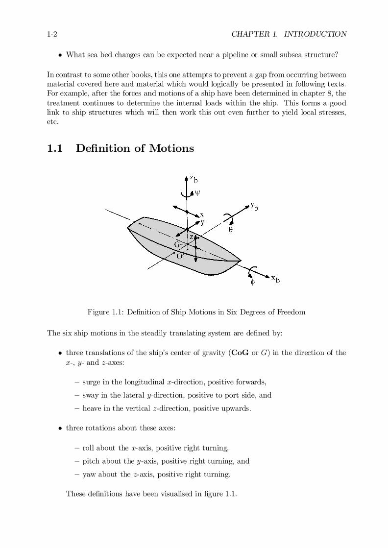
Figure 1.1: De…nition of Ship Motions in Six Degrees of Freedom
The six ship motions in the steadily translating system are de…ned by:
² three translations of the ship’s center of gravity (CoG or G) in the direction of thex-, y- and z-axes:
– surge in the longitudinal x-direction, positive forwards,
– sway in the lateral y-direction, positive to port side, and
– heave in the vertical z-direction, positive upwards.
² three rotations about these axes:
– roll about the x-axis, positive right turning,
– pitch about the y-axis, positive right turning, and
– yaw about the z-axis, positive right turning.
These de…nitions have been visualised in …gure 1.1.
1.2. PROBLEMS OF INTEREST 1-3
Any ship motion is build up from these basic motions. For instance, the vertical motion ofa bridge wing is mainly build up by heave, pitch and roll motions.Another important motion is the vertical relative motion, de…ned as the vertical waveelevation minus the local vertical motion of the ship. This is the motion that one observewhen looking over thee rail downwards to the waves.
1.2 Problems of Interest
This section gives a brief overview of …xed and mobile o¤shore units, such as dredgers,pipe laying vessels, drilling vessels, oil production, storage and o¤-loading units and severaltypes of support and transportation vessels. Their aspects of importance or interest withrespect to the hydromechanical demands are discussed. For a more detailed description ofo¤shore structure problems reference is given to a particular Lecture on Ocean Engineeringby [Wichers, 1992]. Some relevant knowledge of that lecture has been used in this sectiontoo.
1.2.1 Suction Dredgers
Dredging is displacement of soil, carried out under water. The earliest known dredgingactivities by ‡oating equipment took place in the 14th century in the harbor of the DutchHanze city of Kampen. A bucket-type dredging barge was used there to remove the in-creasing sand deposits of the rivers Rhine and IJssel.Generally, this work is carried out nowadays by cutter suction dredgers or trailing suctionhopper dredgers. The cutter suction dredger is moored by means of a spud pile or mooringlines at the stern and by the ladder swing wires at the bow. These dredgers are often usedto dredge trenches for pipe lines and approach channels to harbors and terminals in hardsoil. The trailing suction hopper dredger is dynamically positioned; the dredger uses itspropulsion equipment to proceed over the track.The environmental sea and weather conditions determine:
² the available working time in view of:- the necessity to keep the digging tools in contact with the bottom, such as dippers,
grabs, cutters, suction pipes and trail heads,- the anchorage problems in bad weather, such as breaking adrift from anchors and
bending or breaking of spud piles,- the stability of the discharge equipment, such as ‡oating pipelines and conveyor
belts,- the mooring and stability of barges alongside in the event of currents and/or high
wind velocities and waves and- the overloading of structural elements associated with dredging such as bucket-
ladders or cutter arms,
² maneuverability, especially at strong side winds and strong currents entering at aspeci…c angle, which is important for the dredging slopes,
² problems on slamming of bottom doors of sea-going hopper barges and on jumpingsuction pipes of hopper suction dredgers and
² hopper over‡ow losses due to excessive rolling of the vessel.
1-4 CHAPTER 1. INTRODUCTION
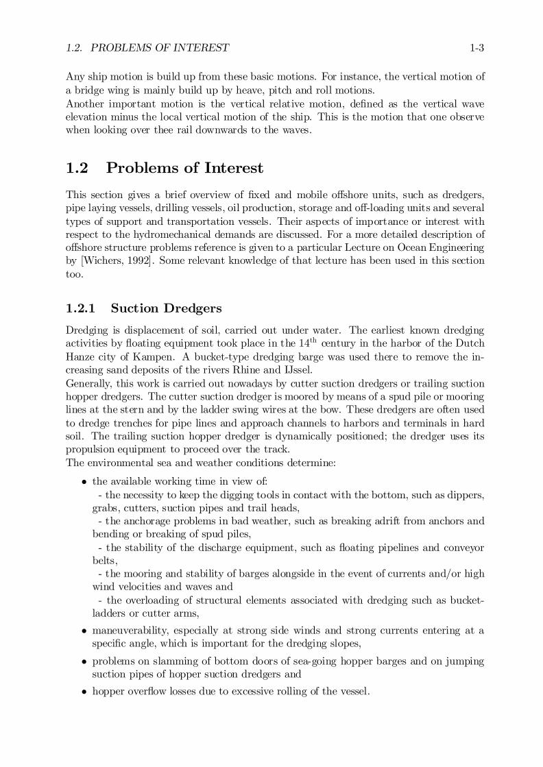
Cutter suction dredgers are moored by means of a spud pile or radially spread steel wires.An important feature of spud pile mooring (see …gure 1.2) is the relative high sti¤ness,compared to other mooring systems. One of the reasons for this high sti¤ness is therequired accurate positioning of the cutter head in the breach. This is necessary for a gooddredging e¢ciency. Another reason is to avoid to high loads on the cutter head and onthe ladder. Since the spud pile can only take a limited load, the workability limit in wavesis at signi…cant wave heights between 0.5 and 1.0 m depending on the size of the dredger,the wave direction and the water depth.
Figure 1.2: Cutter Suction Dredger with Fixed Spud Piles
Cutter suction dredgers may also be equipped with a softer mooring system. In this casethe spud pile is replaced by three radially spread steel wires attached to the spud keeper.This so-called ’Christmas tree’ mooring results in lower loads but larger wave inducedmotions of the dredger. Thus, larger workability has to be traded o¤ against lower cuttinge¢ciency. Other components of the dredging equipment - such as the ‡oating pipe line totransport the slurry, its connection to the dredger and the loads in the ladder - may alsobe limiting factors to the workability of the dredger in waves.Aspects of importance or interest of cutter suction dredgers are:- a realistic mathematical modelling of the soil characteristics for simulations,- the loads in the spud pile, the cutter head and the ladder hoist wires,- the motions of the dredger and the cutter head in the breach and- the loads in the swing wires.
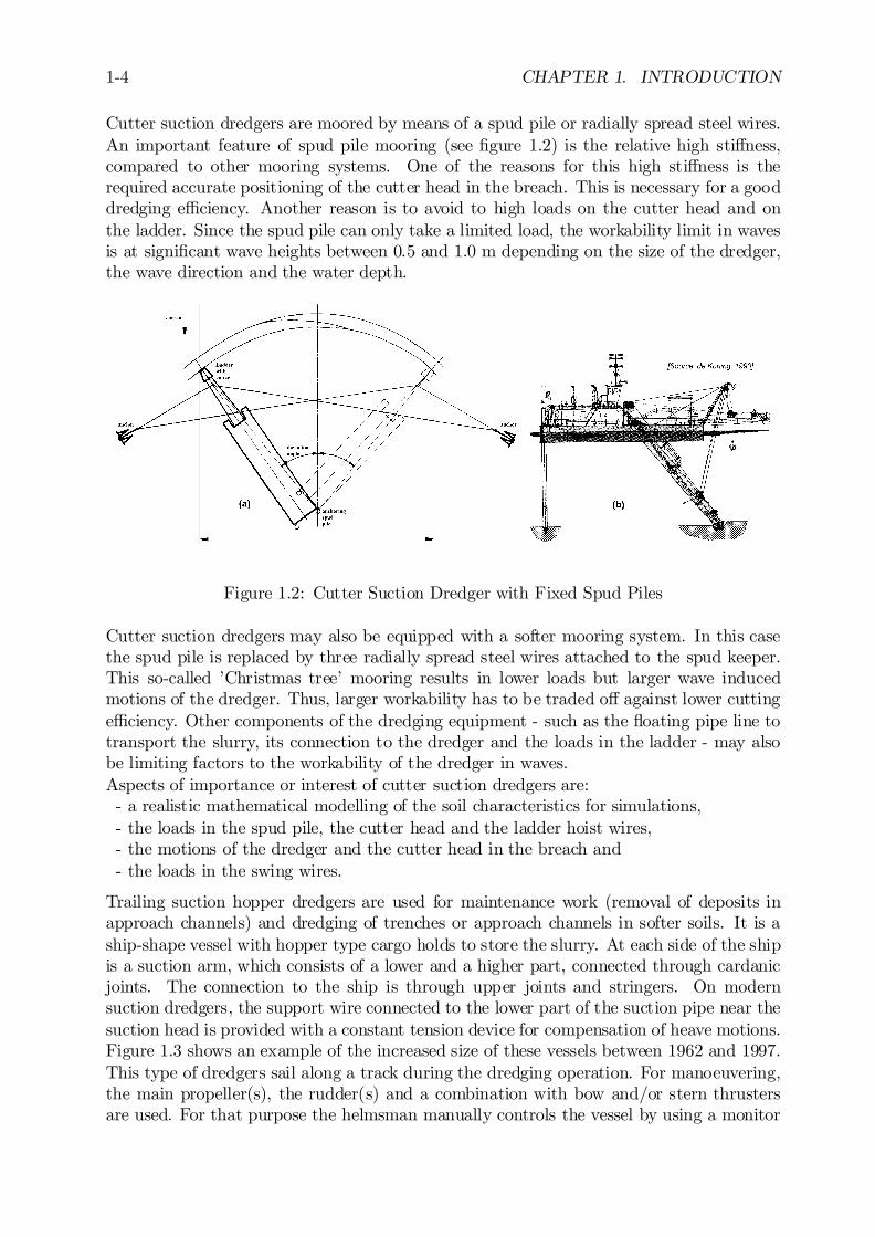
Trailing suction hopper dredgers are used for maintenance work (removal of deposits inapproach channels) and dredging of trenches or approach channels in softer soils. It is aship-shape vessel with hopper type cargo holds to store the slurry. At each side of the shipis a suction arm, which consists of a lower and a higher part, connected through cardanicjoints. The connection to the ship is through upper joints and stringers. On modernsuction dredgers, the support wire connected to the lower part of the suction pipe near thesuction head is provided with a constant tension device for compensation of heave motions.Figure 1.3 shows an example of the increased size of these vessels between 1962 and 1997.This type of dredgers sail along a track during the dredging operation. For manoeuvering,the main propeller(s), the rudder(s) and a combination with bow and/or stern thrustersare used. For that purpose the helmsman manually controls the vessel by using a monitor
1.2. PROBLEMS OF INTEREST 1-5
Figure 1.3: Trailing Cutter Suction Hoppers
showing the actual position of the master drag head and the desired track. Operating innear-shore areas, the vessel will be exposed to waves, wind and current and manual controlof the vessel may be di¢cult. An option is an automatic tracking by means of DP systems.Aspects of importance or interest of trailing suction hopper dredgers are:- the motions of the vessel in waves,- the current forces and the wave drift forces on the vessel,- the low speed tracking capability,- the motions of the suction arms,- the loads in the suction arm connections to the vessel,- the e¤ect and interactions of the thrusters and- the avoidance of backward movements of the suction head at the sea bed.
1.2.2 Pipe Laying Vessels
One of the problems of laying pipes on the sea bed lies in the limited capacity of the pipe toaccept bending stresses. As a result, it is necessary to keep a pipe line under considerableaxial tension during the laying operation otherwise the weight of the span of the pipebetween the vessel and the point of contact of the pipe on the sea bed will cause the pipeto buckle and collapse. The tension in the pipe line is maintained using the anchor linesof the pipe laying vessel. The tension is transferred to the pipe by means of the pipe linetensioner located near the point where the pipe line leaves the vessel. The pipe tensioneris designed to grip the pipe without damaging the pipe coating (concrete) and ease thepipe aft while retaining pipe tension as the vessel is hauled forward by the anchor winches.Forward of the tensioner, additional sections of the pipe line are welded to the alreadyexisting part. Aft of the tensioner, part of the free span of the pipe line is supported by aso-called stinger.
1-6 CHAPTER 1. INTRODUCTION
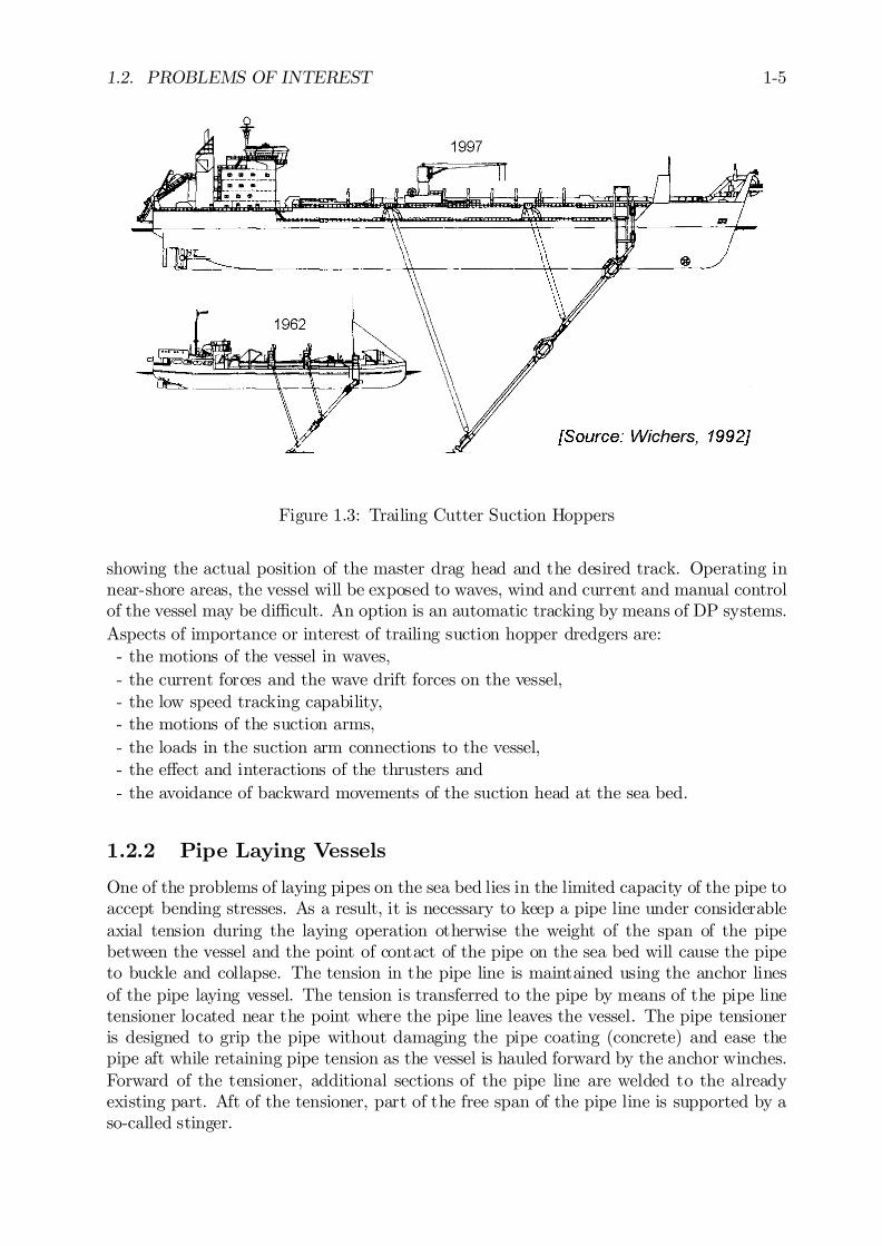
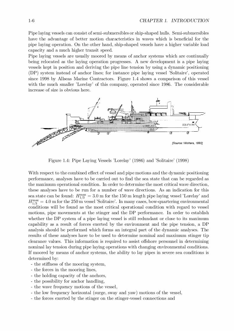
Pipe laying vessels can consist of semi-submersibles or ship-shaped hulls. Semi-submersibleshave the advantage of better motion characteristics in waves which is bene…cial for thepipe laying operation. On the other hand, ship-shaped vessels have a higher variable loadcapacity and a much higher transit speed.Pipe laying vessels are usually moored by means of anchor systems which are continuallybeing relocated as the laying operation progresses. A new development is a pipe layingvessels kept in position and deriving the pipe line tension by using a dynamic positioning(DP) system instead of anchor lines; for instance pipe laying vessel ’Solitaire’, operatedsince 1998 by Allseas Marine Contractors. Figure 1.4 shows a comparison of this vesselwith the much smaller ’Lorelay’ of this company, operated since 1986. The considerableincrease of size is obvious here.
Figure 1.4: Pipe Laying Vessels ’Lorelay’ (1986) and ’Solitaire’ (1998)
With respect to the combined e¤ect of vessel and pipe motions and the dynamic positioningperformance, analyses have to be carried out to …nd the sea state that can be regarded asthe maximum operational condition. In order to determine the most critical wave direction,these analyses have to be run for a number of wave directions. As an indication for thissea state can be found: Hmax
1=3 = 3:0 m for the 150 m length pipe laying vessel ’Lorelay’ andHmax1=3 = 4:0 m for the 250 m vessel ’Solitaire’. In many cases, bow-quartering environmental
conditions will be found as the most critical operational condition with regard to vesselmotions, pipe movements at the stinger and the DP performance. In order to establishwhether the DP system of a pipe laying vessel is still redundant or close to its maximumcapability as a result of forces exerted by the environment and the pipe tension, a DPanalysis should be performed which forms an integral part of the dynamic analyses. Theresults of these analyses have to be used to determine nominal and maximum stinger tipclearance values. This information is required to assist o¤shore personnel in determiningnominal lay tension during pipe laying operations with changing environmental conditions.If moored by means of anchor systems, the ability to lay pipes in severe sea conditions isdetermined by:- the sti¤ness of the mooring system,- the forces in the mooring lines,- the holding capacity of the anchors,- the possibility for anchor handling,- the wave frequency motions of the vessel,- the low frequency horizontal (surge, sway and yaw) motions of the vessel,- the forces exerted by the stinger on the stinger-vessel connections and

1.2. PROBLEMS OF INTEREST 1-7
- the buckling and bending stresses in the pipe line.In case of dynamic positioning, the accuracy of the low speed tracking capability is animportant aspect too.After laying the pipe, it has - in many cases - to be buried in the sea bed or to be coveredby gravel stone. Another possibility is to tow a trencher along the pipe, which acts as ahuge plow. The trencher lifts the pipe, plows a trench and lowers the pipe trench behindit. The sea current takes care of …lling the trench to cover the pipe, as will be discussed inchapter 14.In very extreme conditions the pipe is plugged and lowered to the sea bed, still keepingsu¢cient tension in the pipe in order to avoid buckling. After the pipe is abandoned, thevessel rides out the storm. The ship has to survive a pre-de…ned extreme sea state, forinstance a 100-years storm in the North Sea.
1.2.3 Drilling Vessels
When geological predictions based on seismic surveys have been established that a particu-lar o¤shore area o¤ers promising prospects for …nding oil, a well is drilled to examine thesepredictions. These drilling operations are carried out from barges, ships, semi-submersiblesor jack-up rigs; see …gure 1.5.
Figure 1.5: Ship and Semi-Submersible Type of Drilling Vessel
For ‡oating drilling units it is important that they can work in high sea conditions. Gen-erally, semi-submersibles will have the least vertical motions and hence the highest worka-bility. In order to enhance further the workability of drilling vessels, the vertical motionsof the vessel at the location of the drill string are compensated for by a so-called heave

1-8 CHAPTER 1. INTRODUCTION
compensator. This device is essentially a soft spring by means of which the drill stringis suspended from the drilling tower on the vessel. In this way, the drill string can bemaintained under the required average tension, while the vertical motions of the vessel -and hence of the suspension point of the drill string in the drilling tower - do not result inunduly high drill string tension variations or vertical movement of the drill bit. Also themarine riser is kept under constant tension by means of a riser tensioning system.Horizontal motions are another factor of importance for drilling vessels. As a rule of thumb,the upper end of the drill string may not move more to one side of the center of the drillthan approximately 5 % of the water depth. This places considerable demands on themooring system of the vessels. Semi-submersible drilling vessels are generally moored bymeans of 8 to 12 catenary anchor legs. Drill ships can be moored by means of a spreadmooring system which allows a limited relocation of the vessel’s heading or a by meansof a dynamic positioning (DP) system. The latter system of mooring is also used forsemi-submersible drilling vessels for drilling in water exceeding 200 m depth.Summarized, aspects of importance or interest of drilling vessels are:- the wave frequency vertical motions at the drill ‡oor,- the horizontal motions at the drill ‡oor,- the deck clearance of the work deck of a semi-submersible above a wave crest (air gap),- the vertical relative motions of the water in the moonpool of drill ships,- the damage stability of a drilling semi-submersible,- the forces in the mooring lines,- the mean and low frequency horizontal environmental forces on DP ships and- the thruster e¤ectivity in high waves and currents.
As an example, some limiting criteria for the ship motions - used for the design of the 137m length drilling ship ’Pelican’ in 1972 - were:- ship has to sustain wind gusts up to 100 km/hour,- maximum heel angle: 3 degrees,- roll: 10 degrees in 10 seconds,- pitch: 4 degrees in 10 seconds and- heave: 3.6 meter in 8 seconds.
1.2.4 Oil Production and Storage Units
Crude oil is piped from the wells on the sea bed to the production platform where it isseparated into oil, gas, water and sand. After puri…cation, the water and sand returns tothe sea. Gas can be used for energy on the platform, ‡ared away or brought to shore bymeans of a pipe line. In some cases the produced gas or water is re-injected in the reservoir,in order to enhance the production of crude oil. Crude oil is piped to shore or pumpedtemporarily into storage facilities on or near the platform.
Jackets
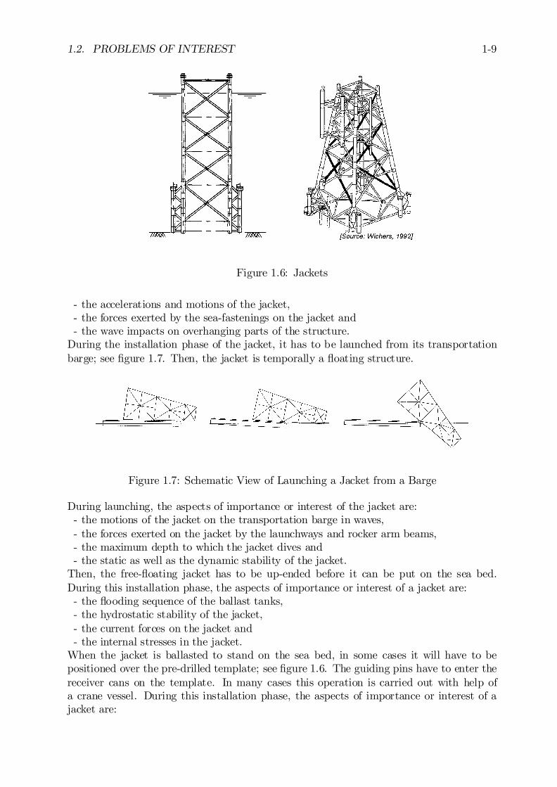
Fixed platforms for oil and gas production are used at water depths ranging to about150 m. In most cases they consist of a jacket, a steel frame construction piled to thesea bed; see …gure 1.6. The jacket supports a sub-frame with production equipment andaccommodation deck on top of it.The jacket has to be transported on a barge to its installation site at sea. During transport,the aspects of importance or interest of a jacket are:
1.2. PROBLEMS OF INTEREST 1-9
Figure 1.6: Jackets
- the accelerations and motions of the jacket,- the forces exerted by the sea-fastenings on the jacket and- the wave impacts on overhanging parts of the structure.
During the installation phase of the jacket, it has to be launched from its transportationbarge; see …gure 1.7. Then, the jacket is temporally a ‡oating structure.
Figure 1.7: Schematic View of Launching a Jacket from a Barge
During launching, the aspects of importance or interest of the jacket are:- the motions of the jacket on the transportation barge in waves,- the forces exerted on the jacket by the launchways and rocker arm beams,- the maximum depth to which the jacket dives and- the static as well as the dynamic stability of the jacket.
Then, the free-‡oating jacket has to be up-ended before it can be put on the sea bed.During this installation phase, the aspects of importance or interest of a jacket are:- the ‡ooding sequence of the ballast tanks,- the hydrostatic stability of the jacket,- the current forces on the jacket and- the internal stresses in the jacket.
When the jacket is ballasted to stand on the sea bed, in some cases it will have to bepositioned over the pre-drilled template; see …gure 1.6. The guiding pins have to enter thereceiver cans on the template. In many cases this operation is carried out with help ofa crane vessel. During this installation phase, the aspects of importance or interest of ajacket are:

1-10 CHAPTER 1. INTRODUCTION
- the motions in waves,- the current forces,- the internal stresses in the jacket,- the loads in the guiding pins and- hoist wave loads in case of crane assisted positioning.
Finally, the jacket will be anchored to the sea bed by means of long steel pipes which arelowered through the pile sleeves and hammered into the sea bed. This can be done by acrane vessel, which also installs the top-side modules.
Jack-Ups
A jack-up is a mobile drilling unit that consists of a self-‡oating, ‡at box-type deck structuresupporting the drilling rig, drilling equipment and accommodation; see …gure 1.8. It standson 3 or 4 vertical legs along which the platform can be self-elevated out of the water toa su¢cient height to remain clear of the highest waves. Drilling operations take place inthe elevated condition with the platform standing on the sea bed. This type of platformis used for drilling operations in water depths up to about 100 m. Jack-ups spend part oftheir life as ‡oating structures. This is when such platforms are towed to a new locationby means of ocean-going tugs. In this mode, the legs are lifted up and extend upwardsover the platform.
Figure 1.8: Jack-Up
Aspects of importance or interest in the towing condition of a jack-up are:- the towing resistance,- the course stability under tow and- the bending stresses in the legs at the point of connection to the deck structure.
These bending stresses are adversely a¤ected by the wave induced roll and pitch motionsof the vessel. In some cases the highest sections of the legs are removed for the towingoperation in order to reduce the bending stresses to acceptable levels.
1.2. PROBLEMS OF INTEREST 1-11
Gravity Base Structures
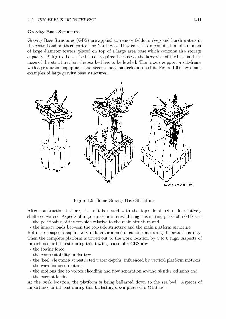
Gravity Base Structures (GBS) are applied to remote …elds in deep and harsh waters inthe central and northern part of the North Sea. They consist of a combination of a numberof large diameter towers, placed on top of a large area base which contains also storagecapacity. Piling to the sea bed is not required because of the large size of the base and themass of the structure, but the sea bed has to be leveled. The towers support a sub-framewith a production equipment and accommodation deck on top of it. Figure 1.9 shows someexamples of large gravity base structures.
Figure 1.9: Some Gravity Base Structures
After construction inshore, the unit is mated with the top-side structure in relativelysheltered waters. Aspects of importance or interest during this mating phase of a GBS are:- the positioning of the top-side relative to the main structure and- the impact loads between the top-side structure and the main platform structure.
Both these aspects require very mild environmental conditions during the actual mating.Then the complete platform is towed out to the work location by 4 to 6 tugs. Aspects ofimportance or interest during this towing phase of a GBS are:- the towing force,- the course stability under tow,- the ’keel’ clearance at restricted water depths, in‡uenced by vertical platform motions,- the wave induced motions,- the motions due to vortex shedding and ‡ow separation around slender columns and- the current loads.
At the work location, the platform is being ballasted down to the sea bed. Aspects ofimportance or interest during this ballasting down phase of a GBS are:
1-12 CHAPTER 1. INTRODUCTION
- the positioning accuracy,- the vertical motions on setting down and- the horizontal wave, wind and current forces.
Floating Production Units
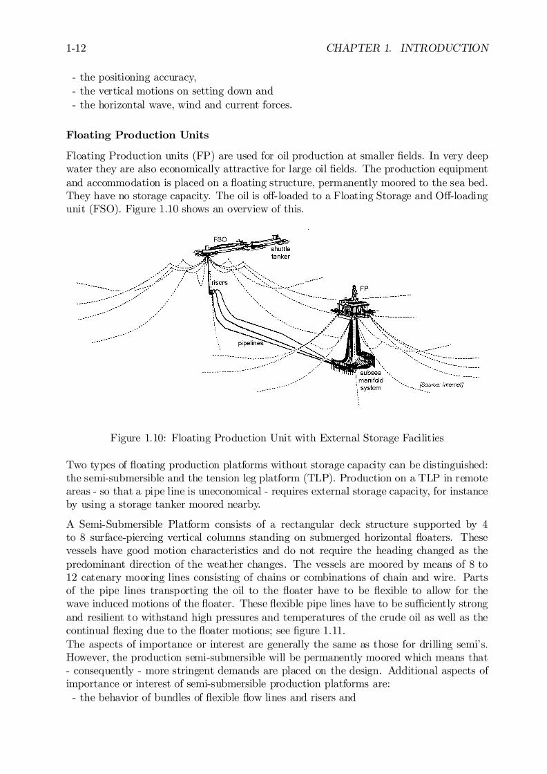
Floating Production units (FP) are used for oil production at smaller …elds. In very deepwater they are also economically attractive for large oil …elds. The production equipmentand accommodation is placed on a ‡oating structure, permanently moored to the sea bed.They have no storage capacity. The oil is o¤-loaded to a Floating Storage and O¤-loadingunit (FSO). Figure 1.10 shows an overview of this.
Figure 1.10: Floating Production Unit with External Storage Facilities
Two types of ‡oating production platforms without storage capacity can be distinguished:the semi-submersible and the tension leg platform (TLP). Production on a TLP in remoteareas - so that a pipe line is uneconomical - requires external storage capacity, for instanceby using a storage tanker moored nearby.
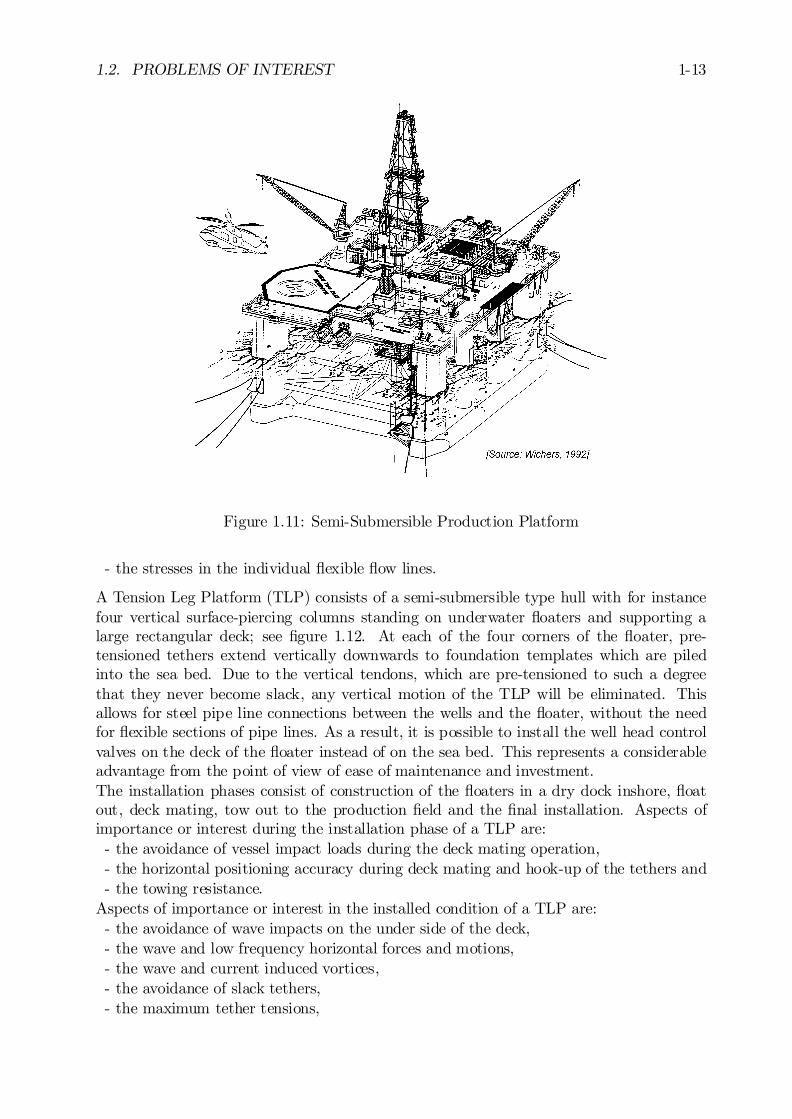
A Semi-Submersible Platform consists of a rectangular deck structure supported by 4to 8 surface-piercing vertical columns standing on submerged horizontal ‡oaters. Thesevessels have good motion characteristics and do not require the heading changed as thepredominant direction of the weather changes. The vessels are moored by means of 8 to12 catenary mooring lines consisting of chains or combinations of chain and wire. Partsof the pipe lines transporting the oil to the ‡oater have to be ‡exible to allow for thewave induced motions of the ‡oater. These ‡exible pipe lines have to be su¢ciently strongand resilient to withstand high pressures and temperatures of the crude oil as well as thecontinual ‡exing due to the ‡oater motions; see …gure 1.11.The aspects of importance or interest are generally the same as those for drilling semi’s.However, the production semi-submersible will be permanently moored which means that- consequently - more stringent demands are placed on the design. Additional aspects ofimportance or interest of semi-submersible production platforms are:- the behavior of bundles of ‡exible ‡ow lines and risers and
1.2. PROBLEMS OF INTEREST 1-13
Figure 1.11: Semi-Submersible Production Platform
- the stresses in the individual ‡exible ‡ow lines.
A Tension Leg Platform (TLP) consists of a semi-submersible type hull with for instancefour vertical surface-piercing columns standing on underwater ‡oaters and supporting alarge rectangular deck; see …gure 1.12. At each of the four corners of the ‡oater, pre-tensioned tethers extend vertically downwards to foundation templates which are piledinto the sea bed. Due to the vertical tendons, which are pre-tensioned to such a degreethat they never become slack, any vertical motion of the TLP will be eliminated. Thisallows for steel pipe line connections between the wells and the ‡oater, without the needfor ‡exible sections of pipe lines. As a result, it is possible to install the well head controlvalves on the deck of the ‡oater instead of on the sea bed. This represents a considerableadvantage from the point of view of ease of maintenance and investment.The installation phases consist of construction of the ‡oaters in a dry dock inshore, ‡oatout, deck mating, tow out to the production …eld and the …nal installation. Aspects ofimportance or interest during the installation phase of a TLP are:- the avoidance of vessel impact loads during the deck mating operation,- the horizontal positioning accuracy during deck mating and hook-up of the tethers and- the towing resistance.
Aspects of importance or interest in the installed condition of a TLP are:- the avoidance of wave impacts on the under side of the deck,- the wave and low frequency horizontal forces and motions,- the wave and current induced vortices,- the avoidance of slack tethers,- the maximum tether tensions,

1-14 CHAPTER 1. INTRODUCTION
Figure 1.12: Tension Leg Platform
- the behavior of the bundles of the tethers,- the super-harmonics in tether tensions (springing) and- the current and wind forces.
Floating Storage and O¤-loading Units
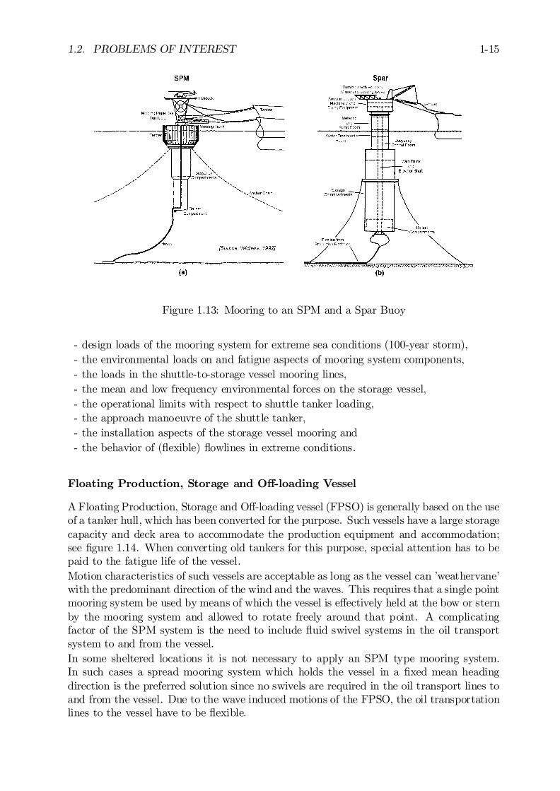
Permanently moored Floating Storage and O¤-loading vessels (FSO’s) are used to storethe produced crude oil. Periodically, the oil is collected and transported to shore by meansof shuttle tankers. For the o¤-loading operation, the shuttle tanker is often moored eitherin tandem with the storage vessel or alongside.Sometimes the stored oil is piped to a Single Point Mooring system (SPM) some distanceaway, to which the shuttle tanker is temporarily moored. A Spar buoy mooring system isan example of this combined o¤shore storage and mooring facility; see …gure 1.13.Generally, due to costs aspects, existing tankers - with sizes ranging from 80 to 200 kDWT -have been used as storage vessels, permanently moored in the neighborhood of a productionplatform or a group of platforms. When converting oil tankers for this purpose, specialattention has to be paid to the remaining fatigue life of this older vessel. Nowadays, thenumber of suitable tankers on the market is relatively small and a trend toward purposebuilt storage vessels is discernible.A factor of prime importance for the operation of these vessels is the continued integrity ofthe mooring system and of the pipe line carrying the crude to the storage vessel. Anotherimportant aspect is the operational limit of the crude oil transfer operation between thestorage vessel and the shuttle tanker. Both these design requirements are mainly deter-mined by the wind, wave and current induced motions, the mooring forces of the storagevessel and those of the shuttle tanker.Aspects of importance or interest of an FSO are:
1.2. PROBLEMS OF INTEREST 1-15
Figure 1.13: Mooring to an SPM and a Spar Buoy
- design loads of the mooring system for extreme sea conditions (100-year storm),- the environmental loads on and fatigue aspects of mooring system components,- the loads in the shuttle-to-storage vessel mooring lines,- the mean and low frequency environmental forces on the storage vessel,- the operational limits with respect to shuttle tanker loading,- the approach manoeuvre of the shuttle tanker,- the installation aspects of the storage vessel mooring and- the behavior of (‡exible) ‡owlines in extreme conditions.
Floating Production, Storage and O¤-loading Vessel
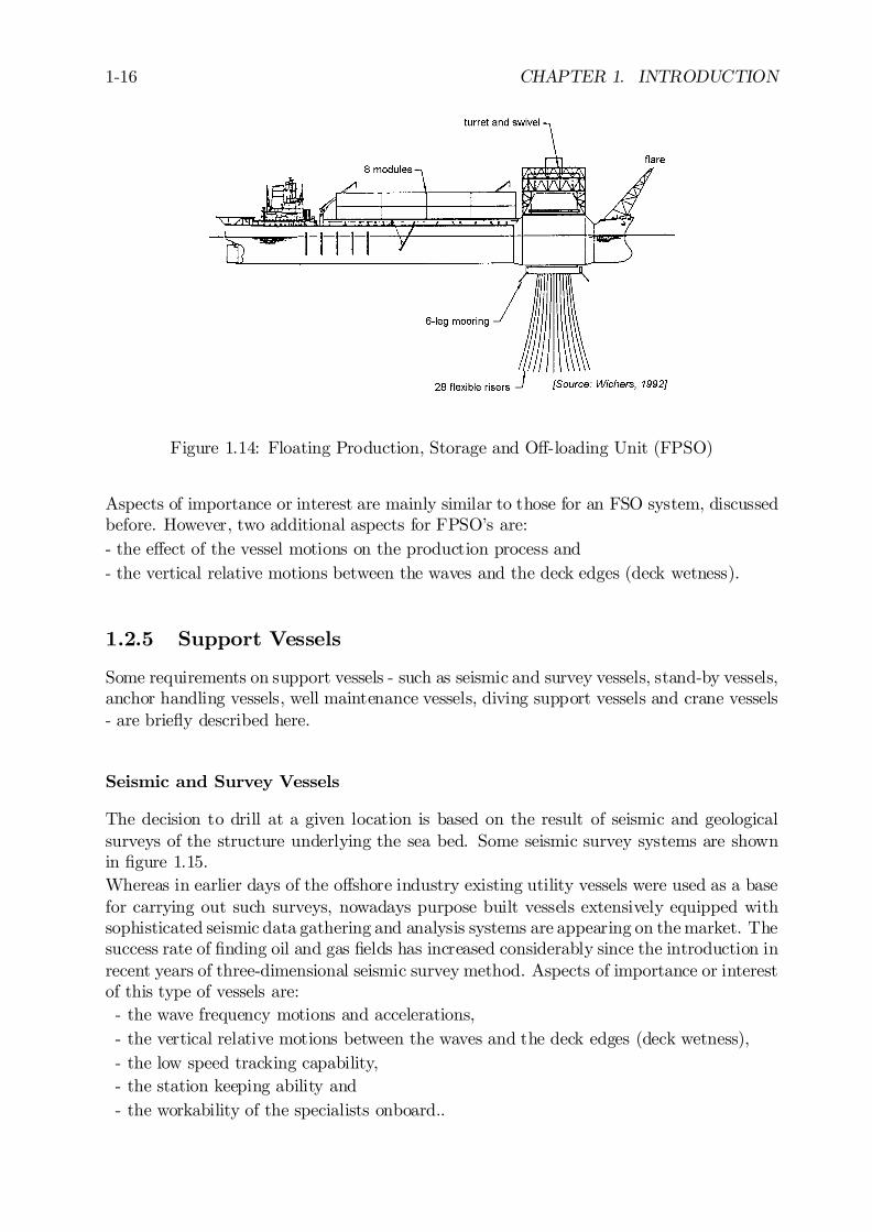
A Floating Production, Storage and O¤-loading vessel (FPSO) is generally based on the useof a tanker hull, which has been converted for the purpose. Such vessels have a large storagecapacity and deck area to accommodate the production equipment and accommodation;see …gure 1.14. When converting old tankers for this purpose, special attention has to bepaid to the fatigue life of the vessel.Motion characteristics of such vessels are acceptable as long as the vessel can ’weathervane’with the predominant direction of the wind and the waves. This requires that a single pointmooring system be used by means of which the vessel is e¤ectively held at the bow or sternby the mooring system and allowed to rotate freely around that point. A complicatingfactor of the SPM system is the need to include ‡uid swivel systems in the oil transportsystem to and from the vessel.In some sheltered locations it is not necessary to apply an SPM type mooring system.In such cases a spread mooring system which holds the vessel in a …xed mean headingdirection is the preferred solution since no swivels are required in the oil transport lines toand from the vessel. Due to the wave induced motions of the FPSO, the oil transportationlines to the vessel have to be ‡exible.
1-16 CHAPTER 1. INTRODUCTION
Figure 1.14: Floating Production, Storage and O¤-loading Unit (FPSO)
Aspects of importance or interest are mainly similar to those for an FSO system, discussedbefore. However, two additional aspects for FPSO’s are:- the e¤ect of the vessel motions on the production process and- the vertical relative motions between the waves and the deck edges (deck wetness).
1.2.5 Support Vessels
Some requirements on support vessels - such as seismic and survey vessels, stand-by vessels,anchor handling vessels, well maintenance vessels, diving support vessels and crane vessels- are brie‡y described here.
Seismic and Survey Vessels
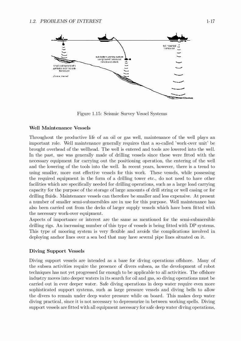
The decision to drill at a given location is based on the result of seismic and geologicalsurveys of the structure underlying the sea bed. Some seismic survey systems are shownin …gure 1.15.Whereas in earlier days of the o¤shore industry existing utility vessels were used as a basefor carrying out such surveys, nowadays purpose built vessels extensively equipped withsophisticated seismic data gathering and analysis systems are appearing on the market. Thesuccess rate of …nding oil and gas …elds has increased considerably since the introduction inrecent years of three-dimensional seismic survey method. Aspects of importance or interestof this type of vessels are:- the wave frequency motions and accelerations,- the vertical relative motions between the waves and the deck edges (deck wetness),- the low speed tracking capability,- the station keeping ability and- the workability of the specialists onboard..
1.2. PROBLEMS OF INTEREST 1-17
Figure 1.15: Seismic Survey Vessel Systems
Well Maintenance Vessels
Throughout the productive life of an oil or gas well, maintenance of the well plays animportant role. Well maintenance generally requires that a so-called ’work-over unit’ bebrought overhead of the wellhead. The well is entered and tools are lowered into the well.In the past, use was generally made of drilling vessels since these were …tted with thenecessary equipment for carrying out the positioning operation, the entering of the welland the lowering of the tools into the well. In recent years, however, there is a trend tousing smaller, more cost e¤ective vessels for this work. These vessels, while possessingthe required equipment in the form of a drilling tower etc., do not need to have otherfacilities which are speci…cally needed for drilling operations, such as a large load carryingcapacity for the purpose of the storage of large amounts of drill string or well casing or fordrilling ‡uids. Maintenance vessels can therefore be smaller and less expensive. At presenta number of smaller semi-submersibles are in use for this purpose. Well maintenance hasalso been carried out from the decks of larger supply vessels which have been …tted withthe necessary work-over equipment.Aspects of importance or interest are the same as mentioned for the semi-submersibledrilling rigs. An increasing number of this type of vessels is being …tted with DP systems.This type of mooring system is very ‡exible and avoids the complications involved indeploying anchor lines over a sea bed that may have several pipe lines situated on it.
Diving Support Vessels
Diving support vessels are intended as a base for diving operations o¤shore. Many ofthe subsea activities require the presence of divers subsea, as the development of robottechniques has not yet progressed far enough to be applicable to all activities. The o¤shoreindustry moves into deeper waters in its search for oil and gas, so diving operations must becarried out in ever deeper water. Safe diving operations in deep water require even moresophisticated support systems, such as large pressure vessels and diving bells to allowthe divers to remain under deep water pressure while on board. This makes deep waterdiving practical, since it is not necessary to depressurize in between working spells. Divingsupport vessels are …tted with all equipment necessary for safe deep water diving operations,
1-18 CHAPTER 1. INTRODUCTION
involving a number of divers simultaneously. Besides sophisticated diving equipment, suchvessels are often equipped with DP systems. Since the divers operating on the sea beddepend on the vessel, high demands are placed on the integrity of the DP systems and onthe motion characteristics of such vessels in waves.Aspects of importance or interest of diving support vessels are:- the horizontal wind, wave and current loads,- the wave frequency motions and accelerations,- the vertical relative motions in the moonpool,- the e¤ect of current and wave frequency motions on the thruster performances and- the station keeping ability.
Crane Vessels
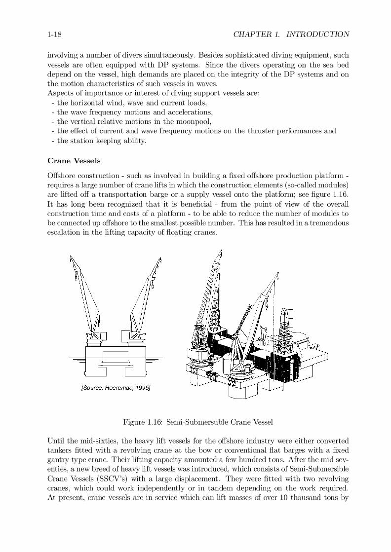
O¤shore construction - such as involved in building a …xed o¤shore production platform -requires a large number of crane lifts in which the construction elements (so-called modules)are lifted o¤ a transportation barge or a supply vessel onto the platform; see …gure 1.16.It has long been recognized that it is bene…cial - from the point of view of the overallconstruction time and costs of a platform - to be able to reduce the number of modules tobe connected up o¤shore to the smallest possible number. This has resulted in a tremendousescalation in the lifting capacity of ‡oating cranes.
Figure 1.16: Semi-Submersuble Crane Vessel
Until the mid-sixties, the heavy lift vessels for the o¤shore industry were either convertedtankers …tted with a revolving crane at the bow or conventional ‡at barges with a …xedgantry type crane. Their lifting capacity amounted a few hundred tons. After the mid sev-enties, a new breed of heavy lift vessels was introduced, which consists of Semi-SubmersibleCrane Vessels (SSCV’s) with a large displacement. They were …tted with two revolvingcranes, which could work independently or in tandem depending on the work required.At present, crane vessels are in service which can lift masses of over 10 thousand tons by

1.2. PROBLEMS OF INTEREST 1-19
using the two cranes simultaneously. Due to the superior motion behavior of the semi-submersible hull form in waves, the workability with respect to crane operations increasedtremendously.Subjects of prime importance for crane operations o¤shore are the impact load that canoccur as a load is taken o¤ a transportation barge, because of the di¤erent vertical velocitiesof the two vessels. In an environment with waves the barge and the heavy lift crane vesselcarry out wave frequency motions. As the lift is taken o¤ the barge, it will carry outvertical motions which are dictated by the crane vessel motion characteristics. The barge,on the other hand, also carries out wave frequency motions which - in general - will notbe in phase with the motions of the load in the hook. When the load is just clearing thebarge, this will result in impacting of the load on the barge. This may lead to damage ofthe load, the barge or the crane vessel or even all three of them. The prime concern thenis to reduce the risk that a critical impact occurs. This can be in‡uenced by the design ofthe crane vessel, for instance by including the ability to transport the load on the deck ofthe crane vessel, but also by operational procedures and aids such as quick de-ballastingsystems. Besides the occurrence of impact loads which are mainly a¤ected by the verticalmotion response to waves, the horizontal motions of the crane vessel are of importancewith respect to the feasibility of accurate positioning of the load onto the platform underconstruction. These motions are a¤ected by environmental loads due to wind, waves andcurrent acting on the crane vessel, by the design and layout of the mooring or positioningsystem and by the dynamics of the load hanging in the crane.Thus, aspects of importance or interest of crane vessels are:- the vertical crane hook motions in waves,- the horizontal positioning accuracy of the hook load,- the impacts on lift-o¤ and set-down of the load,- the deck load capacity,- the transit speed and- the mooring forces.
For the DP system extensive investigations have been carried out into the following aspectsof the station keeping ability:- the thruster-hull, thruster-thruster and thruster-current interactions,- the drift forces due to waves,- the current forces and- the wind forces.
1.2.6 Transportation Vessels
Some types of transportation vessels are discussed here: shuttle tankers, heavy lift trans-portation vessels, launch barges, ocean-going tugs, supply vessels and personnel transfervessels.
Shuttle Tankers
From the storage facilities the oil is transported to shore by means of pipelines or shuttletankers. These shuttle tankers are temporarily moored close to the storage system bymeans of a single point mooring (SPM) system, mooring in tandem (see …gure 1.17) oralongside the storage vessel or by means of a DP system.
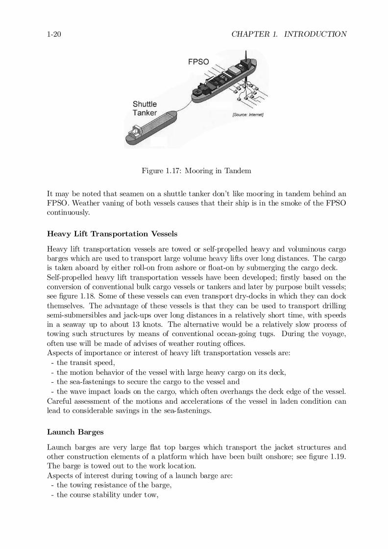
1-20 CHAPTER 1. INTRODUCTION
Figure 1.17: Mooring in Tandem
It may be noted that seamen on a shuttle tanker don’t like mooring in tandem behind anFPSO. Weather vaning of both vessels causes that their ship is in the smoke of the FPSOcontinuously.
Heavy Lift Transportation Vessels
Heavy lift transportation vessels are towed or self-propelled heavy and voluminous cargobarges which are used to transport large volume heavy lifts over long distances. The cargois taken aboard by either roll-on from ashore or ‡oat-on by submerging the cargo deck.Self-propelled heavy lift transportation vessels have been developed; …rstly based on theconversion of conventional bulk cargo vessels or tankers and later by purpose built vessels;see …gure 1.18. Some of these vessels can even transport dry-docks in which they can dockthemselves. The advantage of these vessels is that they can be used to transport drillingsemi-submersibles and jack-ups over long distances in a relatively short time, with speedsin a seaway up to about 13 knots. The alternative would be a relatively slow process oftowing such structures by means of conventional ocean-going tugs. During the voyage,often use will be made of advises of weather routing o¢ces.Aspects of importance or interest of heavy lift transportation vessels are:- the transit speed,- the motion behavior of the vessel with large heavy cargo on its deck,- the sea-fastenings to secure the cargo to the vessel and- the wave impact loads on the cargo, which often overhangs the deck edge of the vessel.
Careful assessment of the motions and accelerations of the vessel in laden condition canlead to considerable savings in the sea-fastenings.
Launch Barges
Launch barges are very large ‡at top barges which transport the jacket structures andother construction elements of a platform which have been built onshore; see …gure 1.19.The barge is towed out to the work location.Aspects of interest during towing of a launch barge are:- the towing resistance of the barge,- the course stability under tow,

1.2. PROBLEMS OF INTEREST 1-21
Figure 1.18: Heavy Lift Float-On Float-O¤ Vessel
- the motions and accelerations of the barge and- the forces on sea-fastenings holding the jacket on the barge.
At the work location, the barge is held stationary, while the jacket structure is end-launchedo¤ the barge. During this launching operation - see …gure 1.7 - the barge is not tightlyheld by the tugs since, as the jacket is launched, the barge will carry out relatively violentmotions and be pushed away over quite a distance. The launching operation is initiatedafter the sea-fastenings have been cut loose and the jacket is only resting on the launchways.By ballasting the barge to the speci…ed trim angle and with initial winch pulling, the jacketwill start to slide over the launchways.Aspects of importance or interest for the barge during launching are:- the maximum depth of submergence of the aft end of the barge,- the ballast distribution,- the friction of the launchways,- the angle of rotation of the rocker beams,- the rocker beam forces and- the stability during the launch.
Very slender structures are sometimes side-launched. Some jackets have been designed tobe crane-lifted o¤ the barge by a crane barge or a crane vessel. Then the impact loads onjacket and barge at the moment of lift-o¤ is an aspect of importance.
Tugs and Supply Vessels
Tugs and supply vessels are the ’workhorses’ of the o¤shore industry.Tugs are used to tow all types of ‡oating o¤shore equipment out to the work location andare in many cases a permanent ’companion’; see …gure 8.32. Large deep-sea tugs are usedfor long distance towing and smaller tugs are employed for short range towing operations.A special type of tug is the so-called anchor handling tug. This vessel is used to positionand re-position the anchors of drilling rigs and in stand-by mode it is used for a pipe layingvessel as it proceeds along the pipe line trajectory.
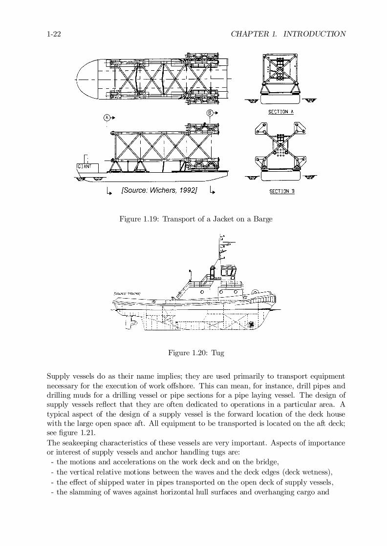
1-22 CHAPTER 1. INTRODUCTION
Figure 1.19: Transport of a Jacket on a Barge
Figure 1.20: Tug
Supply vessels do as their name implies; they are used primarily to transport equipmentnecessary for the execution of work o¤shore. This can mean, for instance, drill pipes anddrilling muds for a drilling vessel or pipe sections for a pipe laying vessel. The design ofsupply vessels re‡ect that they are often dedicated to operations in a particular area. Atypical aspect of the design of a supply vessel is the forward location of the deck housewith the large open space aft. All equipment to be transported is located on the aft deck;see …gure 1.21.The seakeeping characteristics of these vessels are very important. Aspects of importanceor interest of supply vessels and anchor handling tugs are:- the motions and accelerations on the work deck and on the bridge,- the vertical relative motions between the waves and the deck edges (deck wetness),- the e¤ect of shipped water in pipes transported on the open deck of supply vessels,- the slamming of waves against horizontal hull surfaces and overhanging cargo and

1.2. PROBLEMS OF INTEREST 1-23
Figure 1.21: Supply Vessel
- the station keeping near platforms during (un)loading and anchor handling operations.
Personnel Transfer Vessels
Helicopters are the most important means to transfer personnel safely and quickly fromand to o¤shore units and ships. For this, these structures have to be equipped with ahelicopter deck. Also, supply vessels are still used to tranfer personnel. Figure 1.22 showsa special crew boat for personnel transfer, with a length of 31 meter, which can transport55 passengers with a cruising speed of 20 knots. However, in the North Sea areas, thehelicopter is the most common vehicle for personnel transfer.
Figure 1.22: Crew Boat
For long distances, helicopters are used to transfer pilots to and from ships too. Pilot vesselsare used generally for short distances. Conventional types of pilot vessels operate withservice speeds under 20 knots. Generally, they are operating safely in weather conditionsup to sea states de…ned by Beaufort 9 or 10. Figure 1.23 shows some modern types ofthese vessels: a planing hull ship and small waterplane area twin hull (SWATH) ship, withmaximum speeds of about 28 knots. At a reduced speed, they can operate safely in weatherconditions up to Beaufort 8.
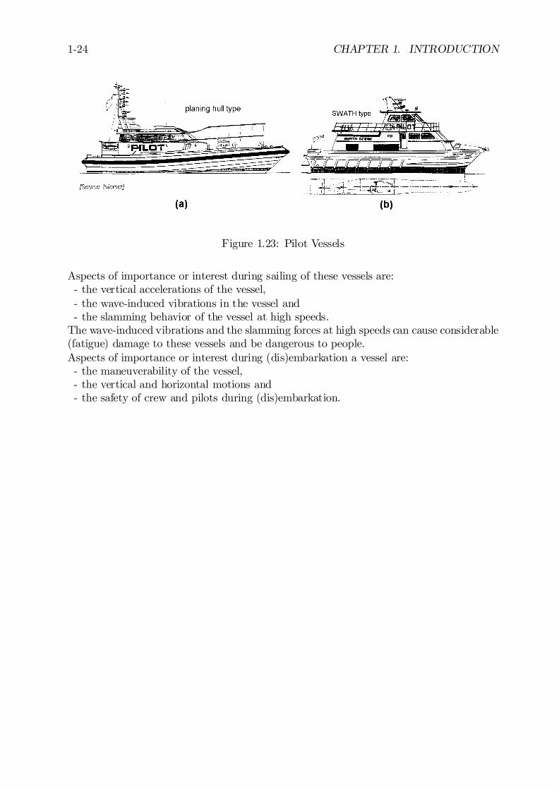
1-24 CHAPTER 1. INTRODUCTION
Figure 1.23: Pilot Vessels
Aspects of importance or interest during sailing of these vessels are:- the vertical accelerations of the vessel,- the wave-induced vibrations in the vessel and- the slamming behavior of the vessel at high speeds.
The wave-induced vibrations and the slamming forces at high speeds can cause considerable(fatigue) damage to these vessels and be dangerous to people.Aspects of importance or interest during (dis)embarkation a vessel are:- the maneuverability of the vessel,- the vertical and horizontal motions and- the safety of crew and pilots during (dis)embarkation.
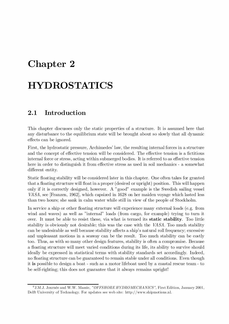
Chapter 2
HYDROSTATICS
2.1 Introduction
This chapter discusses only the static properties of a structure. It is assumed here thatany disturbance to the equilibrium state will be brought about so slowly that all dynamice¤ects can be ignored.
First, the hydrostatic pressure, Archimedes’ law, the resulting internal forces in a structureand the concept of e¤ective tension will be considered. The e¤ective tension is a …ctitiousinternal force or stress, acting within submerged bodies. It is referred to as e¤ective tensionhere in order to distinguish it from e¤ective stress as used in soil mechanics - a somewhatdi¤erent entity.
Static ‡oating stability will be considered later in this chapter. One often takes for grantedthat a ‡oating structure will ‡oat in a proper (desired or upright) position. This will happenonly if it is correctly designed, however. A ”good” example is the Swedish sailing vesselVASA, see [Franzen, 1962], which capsized in 1628 on her maiden voyage which lasted lessthan two hours; she sank in calm water while still in view of the people of Stockholm.
In service a ship or other ‡oating structure will experience many external loads (e.g. fromwind and waves) as well as ”internal” loads (from cargo, for example) trying to turn itover. It must be able to resist these, via what is termed its static stability. Too littlestability is obviously not desirable; this was the case with the VASA. Too much stabilitycan be undesirable as well because stability a¤ects a ship’s natural roll frequency; excessiveand unpleasant motions in a seaway can be the result. Too much stability can be costlytoo. Thus, as with so many other design features, stability is often a compromise. Becausea ‡oating structure will meet varied conditions during its life, its ability to survive shouldideally be expressed in statistical terms with stability standards set accordingly. Indeed,no ‡oating structure can be guaranteed to remain stable under all conditions. Even thoughit is possible to design a boat - such as a motor lifeboat used by a coastal rescue team - tobe self-righting; this does not guarantee that it always remains upright!
0J.M.J. Journée and W.W. Massie, ”OFFSHORE HYDROMECHANICS”, First Edition, January 2001,Delft University of Technology. For updates see web site: http://www.shipmotions.nl.
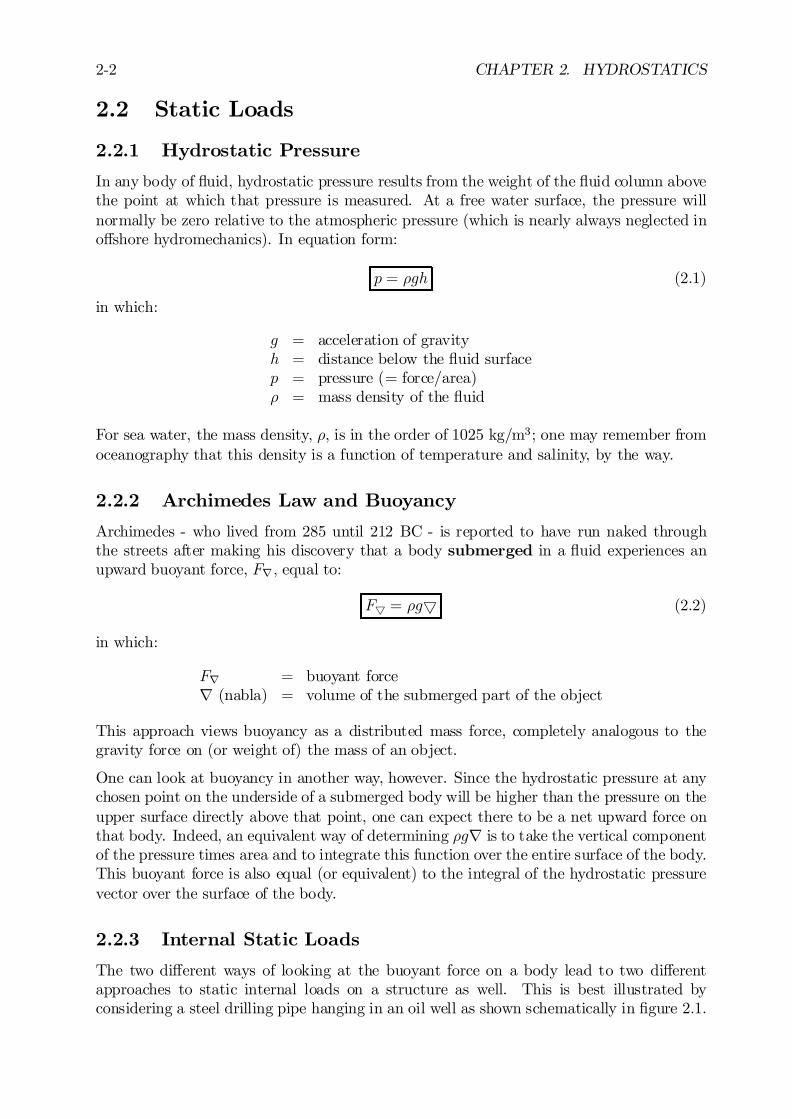
2-2 CHAPTER 2. HYDROSTATICS
2.2 Static Loads
2.2.1 Hydrostatic Pressure
In any body of ‡uid, hydrostatic pressure results from the weight of the ‡uid column abovethe point at which that pressure is measured. At a free water surface, the pressure willnormally be zero relative to the atmospheric pressure (which is nearly always neglected ino¤shore hydromechanics). In equation form:
p = ½gh (2.1)
in which:
g = acceleration of gravityh = distance below the ‡uid surfacep = pressure (= force/area)½ = mass density of the ‡uid
For sea water, the mass density, ½, is in the order of 1025 kg/m3; one may remember fromoceanography that this density is a function of temperature and salinity, by the way.
2.2.2 Archimedes Law and Buoyancy
Archimedes - who lived from 285 until 212 BC - is reported to have run naked throughthe streets after making his discovery that a body submerged in a ‡uid experiences anupward buoyant force, Fr; equal to:
F5 = ½g5 (2.2)
in which:
Fr = buoyant forcer (nabla) = volume of the submerged part of the object
This approach views buoyancy as a distributed mass force, completely analogous to thegravity force on (or weight of) the mass of an object.
One can look at buoyancy in another way, however. Since the hydrostatic pressure at anychosen point on the underside of a submerged body will be higher than the pressure on theupper surface directly above that point, one can expect there to be a net upward force onthat body. Indeed, an equivalent way of determining ½gr is to take the vertical componentof the pressure times area and to integrate this function over the entire surface of the body.This buoyant force is also equal (or equivalent) to the integral of the hydrostatic pressurevector over the surface of the body.
2.2.3 Internal Static Loads
The two di¤erent ways of looking at the buoyant force on a body lead to two di¤erentapproaches to static internal loads on a structure as well. This is best illustrated byconsidering a steel drilling pipe hanging in an oil well as shown schematically in …gure 2.1.
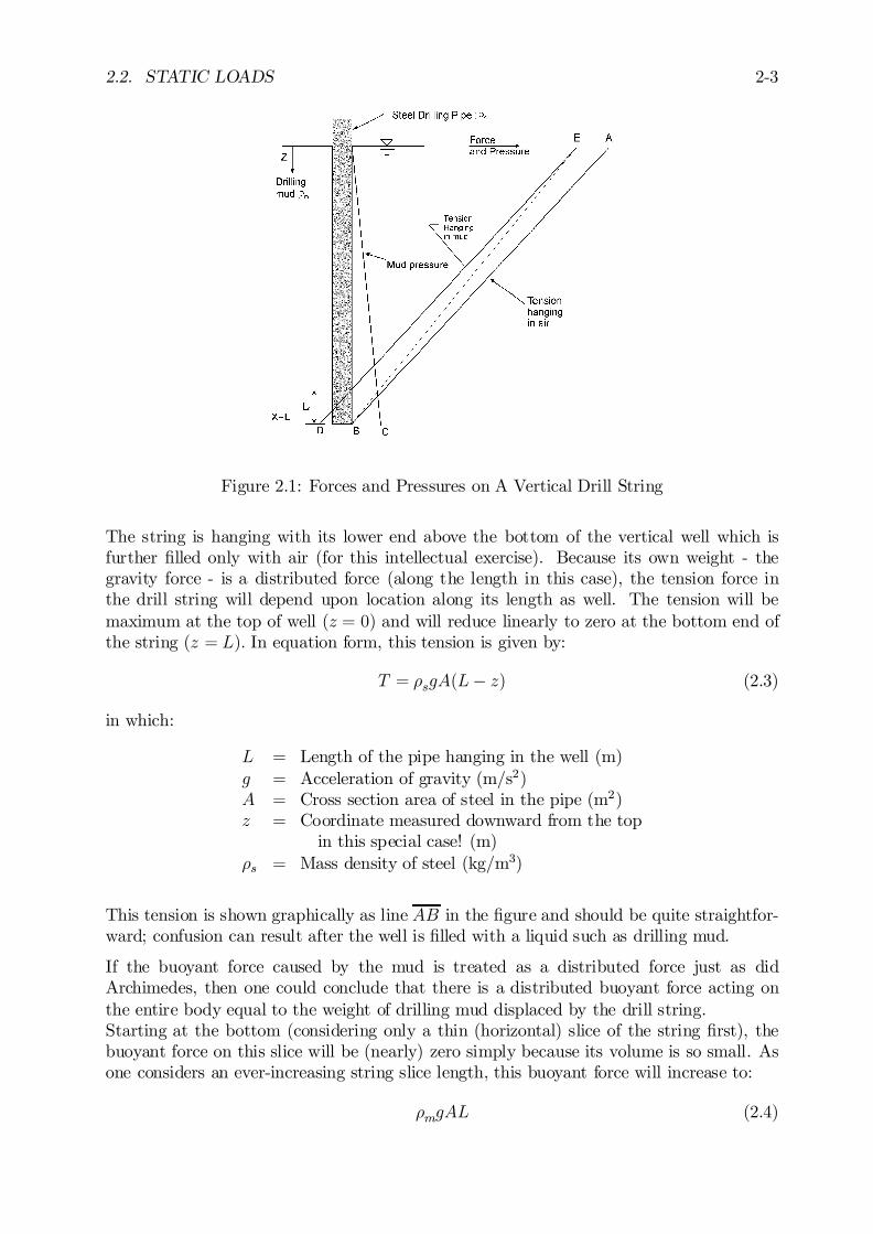
2.2. STATIC LOADS 2-3
Figure 2.1: Forces and Pressures on A Vertical Drill String
The string is hanging with its lower end above the bottom of the vertical well which isfurther …lled only with air (for this intellectual exercise). Because its own weight - thegravity force - is a distributed force (along the length in this case), the tension force inthe drill string will depend upon location along its length as well. The tension will bemaximum at the top of well (z = 0) and will reduce linearly to zero at the bottom end ofthe string (z = L): In equation form, this tension is given by:
T = ½sgA(L¡ z) (2.3)
in which:
L = Length of the pipe hanging in the well (m)g = Acceleration of gravity (m/s2)A = Cross section area of steel in the pipe (m2)z = Coordinate measured downward from the top
in this special case! (m)½s = Mass density of steel (kg/m3)
This tension is shown graphically as line AB in the …gure and should be quite straightfor-ward; confusion can result after the well is …lled with a liquid such as drilling mud.
If the buoyant force caused by the mud is treated as a distributed force just as didArchimedes, then one could conclude that there is a distributed buoyant force acting onthe entire body equal to the weight of drilling mud displaced by the drill string.Starting at the bottom (considering only a thin (horizontal) slice of the string …rst), thebuoyant force on this slice will be (nearly) zero simply because its volume is so small. Asone considers an ever-increasing string slice length, this buoyant force will increase to:
½mgAL (2.4)
2-4 CHAPTER 2. HYDROSTATICS
at the top of the string. Since this buoyant force acts in a direction opposite to the gravityforce, one …nds:
Te = (½s ¡ ½m)gA(L¡ z) (2.5)
Since ½s > ½m, Te will be generally be greater than zero as well, but will be less than T;above. Te is often referred to as the e¤ective tension. It, too, varies linearly from amaximum value at z = 0 to zero at z = L and indicated by line EB in the …gure. Ingeneral the e¤ective tension is based upon the submerged weight of the body. This isthe weight of the body in air minus the buoyant force acting on it. It can be computed forhomogeneous bodies in water using a density of (½b ¡ ½) ; where ½b is the mass density ofthe body.If, on the other hand, one treats the buoyant force as the resultant of pressures acting onthe surface of the body - the drill string in this case, then one …nds …rst that the pressureson the (vertical) drill string walls are in equilibrium and contribute no vertical force. Thedrill string does experience a vertical force at its bottom end which is equal to:
Fz = ½mgAL (2.6)
This concentrated vertical upward force combines with the distributed weight of the drillstring by shifting line AB in the …gure to position DE: One discovers now that the lowersection of the drill string is in compression instead of tension! The length that is incompression can be computed:
Lc =½m½sL (2.7)
One can also conclude that there will be no axial force in the drill string at an elevation Lcabove its bottom end and that the entire length below that point will be in compression.This does not agree with what was found when the buoyant force was treated as Archimedeshad done, above.
It is easiest to resolve this apparent dilemma by examining a slightly di¤erent situation.Consider a solid body which has the same density as water; an atheletic swimmer is areasonable approximation of this. Considering buoyancy as a distributed force (in theArchimedian sense) would now yield an e¤ective tension in this swimmer’s body thatwould be zero, independent of the depth to which he or she might happen to dive. Asanyone who has suddenly plunged into a pool has probably discovered, this is not thecase. Indeed, as one dives rapidly deeper into the water the external pressure trying tocrush one’s body only gets larger. This observation supports the external pressure form ofbuoyancy argument rather than Archimedes’ approach. Apparently, the external pressureform is better for revealing the actual true stress in the submerged body, just as with therapidly diving swimmer.
On the other hand, the e¤ective tension - resulting from the distributed force approachto buoyancy - also has its uses even though the e¤ective tension will not be measuredby a strain gauge mounted on the submerged object. Consider a given length of metalchain hanging between two …xed points in air. The tension at any point in that chain isdependent upon the chain’s weight per unit length. If the chain were hung in the samecon…guration under water, one would expect the tension to be lower. That will indeed bethe case; the tension force between adjacent links of the chain now becomes the e¤ectivetension.
2.2. STATIC LOADS 2-5
2.2.4 Drill String Buckling
Returning to the hanging drill string problem posed above, an important structural engi-neering question involves the buckling behavior of its lower part. It was shown above thatthe actual axial force in the lower Lc meters of the drill string is compressive. Since themud surrounding this string provides no lateral support, a structural engineer would feelvery justi…ed in applying the Euler column buckling formula:
PcrA=
¼2E
(Lc=r)2(2.8)
in which:
Pcr = Critical buckling load (N)A = Cross section area of the column (m2)E = Material elastic modulus (N/m2)Lc=r = Column slenderness ratio (-)
to determine that if Lc is long enough, the drill string segment should buckle.Another structural engineer can argue that the e¤ective tension in this drill string segmentis positive over its entire length; a structure in tension will not buckle.
An independent approach is needed to resolve this discussion. An independent theoreticalapproach follows from potential energy changes. How does the potential energy of the mudplus drill string change as the drill string buckles? Considering …rst the drill string steel, ifit buckles, then the bottom end of the drill string will move up very slightly, thus raisingits center of gravity and thereby increasing the total potential energy of the string. Themud, on the other hand, loses a minute amount of potential energy as it compensates forthis drill string movement. Since the drill string has a higher density than the mud, thestring gains more potential energy than the mud loses. Potential energy is thus created ifthe drill string buckles! Any type of engineer should recognize that this cannot happen;One cannot expect the drill string to buckle when it is hanging freely in the mud-…lledwell.Apparently two conditions must be met before a long slender submerged object will buckle:
- it must actually be under compression and- its e¤ective tension must be negative.
These criteria can be checked by considering a chain instead of the drill string hanging in thewell. The positive weight minus buoyant force of each link will cause there to be a positivee¤ective tension between each link. However, since each link is also essentially surroundedby drilling ‡uid exerting an external pressure on its surface, it should be equally obviousthat the material in each of the deepest links (at least) will be experiencing a compressiveforce, just like the diving swimmer, above.Another check can be made by considering - at least intellectually - a drilling string with adensity which is less than that of the drilling mud. One can see immediately from equation2.5 that the e¤ective tension will now be negative. Indeed, the sting will buckle as soon asa long enough segment is lowered into the drilling mud.
Of course the force situation in the drill string changes as soon as a point of a drill bit toothis lowered to the hole bottom. From that moment on, an extra upward force is exerted onthe base of the drill string so that the e¤ective tension becomes negative in the lowest part
2-6 CHAPTER 2. HYDROSTATICS
of the string. This negative e¤ective tension segment gets longer in direct proportion tothe well bottom contact force. If this contact force gets big enough, then the lower segmentof the drill string will obviously buckle.
An experimental test of drill string buckling has been carried out by D. Brussmann inGermany. Unfortunately, his work is not reported in the open literature, but one of theauthors has seen photos of his test. The photos show - in contrast to the conclusionsabove - that the drill string will buckle even before it touches the bottom of the well. Thisobviously makes the confusion complete and can initiate an interesting discussion of whatto believe of all this.More than a century ago, a famous hydraulic engineer (in his time), C.M. Allen is reportedto have remarked: ”When the theory and the experiment do not agree, then take a goodhard look at the theory.” In any case, a safe conclusion to all this is that new - con…rmatorytests are needed. These are being carried out at the Delft University of Technology.
2.2.5 Pipeline on Sea Bed
Consider the horizontal force balance on an isolated segment of a horizontal pipe submergedin (and completely surrounded by) a ‡uid; the ‡uid pressure acting at the depth of thecenter line of the pipe is p: The mathematics is simplest if one makes two simpli…cations:
1. The pipe has a rectangular cross section with height 1; this makes all forces eitherhorizontal or vertical.
2. The pressure change between the top and bottom of the pipe - at least that on thevertical surfaces of the pipe - can be neglected. This is not acceptable if the verticalequilibrium is considered; it is the pressure di¤erence the top and bottom surfaceswhich yields the buoyant force. These vertical forces have no e¤ect on the horizontalequilibrium of interest here, however.
Consider …rst a straight pipe. The pressure forces on each side of the pipe will be opposite,equal and have identical lines of action; they will cancel. The same will be true of thehydrostatic pressure forces on the pipe ends. Of course, all these external pressures willcause compressive loadings within the pipe wall, but there is no resultant horizontal forceand no (internal) moment in a straight segment of an isolated horizontal pipe (or bar).This means that no matter how long the structure is, and even though it is obviouslysubjected to a potentially large compressive load, no moments are generated. This is quitelike the case with the vertical drill string. The e¤ective tension in this pipe is now zeroand it does not buckle. This is in agreement with the two ’rules’ given above.Even if the pipe has an initial curvature, one can work out the pressure force balance todiscover that there is still no resulting moment in the pipe; it still will not buckle! Instead,just as one might expect when the limit Te = 0 is reached in the above ’rules’, the pipe hascome to a neutral state of equilibrium.
2.3 Static Floating Stability
The static stability of a ‡oating structure encompasses the up-righting properties of thestructure when it is brought out of equilibrium or balance by a disturbance in the form
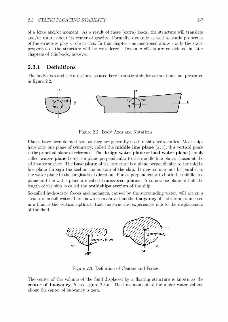
2.3. STATIC FLOATING STABILITY 2-7
of a force and/or moment. As a result of these (extra) loads, the structure will translateand/or rotate about its center of gravity. Formally, dynamic as well as static propertiesof the structure play a role in this. In this chapter - as mentioned above - only the staticproperties of the structure will be considered. Dynamic e¤ects are considered in laterchapters of this book, however.
2.3.1 De…nitions
The body axes and the notations, as used here in static stability calculations, are presentedin …gure 2.2.
Figure 2.2: Body Axes and Notations
Planes have been de…ned here as they are generally used in ship hydrostatics. Most shipshave only one plane of symmetry, called the middle line plane (x; z); this vertical planeis the principal plane of reference. The design water plane or load water plane (simplycalled water plane here) is a plane perpendicular to the middle line plane, chosen at thestill water surface. The base plane of the structure is a plane perpendicular to the middleline plane through the keel or the bottom of the ship. It may or may not be parallel tothe water plane in the longitudinal direction. Planes perpendicular to both the middle lineplane and the water plane are called transverse planes. A transverse plane at half thelength of the ship is called the amidships section of the ship.
So-called hydrostatic forces and moments, caused by the surrounding water, will act on astructure in still water. It is known from above that the buoyancy of a structure immersedin a ‡uid is the vertical upthrust that the structure experiences due to the displacementof the ‡uid.
Figure 2.3: De…nition of Centers and Forces
The center of the volume of the ‡uid displaced by a ‡oating structure is known as thecenter of buoyancy B, see …gure 2.3-a. The …rst moment of the under water volumeabout the center of buoyancy is zero.
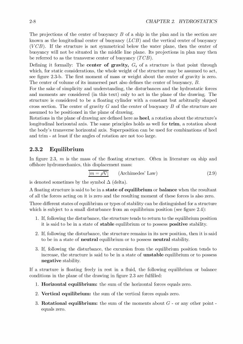
2-8 CHAPTER 2. HYDROSTATICS
The projections of the center of buoyancy B of a ship in the plan and in the section areknown as the longitudinal center of buoyancy (LCB) and the vertical center of buoyancy(V CB). If the structure is not symmetrical below the water plane, then the center ofbuoyancy will not be situated in the middle line plane. Its projections in plan may thenbe referred to as the transverse center of buoyancy (TCB).
De…ning it formally: The center of gravity, G, of a structure is that point throughwhich, for static considerations, the whole weight of the structure may be assumed to act,see …gure 2.3-b. The …rst moment of mass or weight about the center of gravity is zero.The center of volume of its immersed part also de…nes the center of buoyancy, B:For the sake of simplicity and understanding, the disturbances and the hydrostatic forcesand moments are considered (in this text) only to act in the plane of the drawing. Thestructure is considered to be a ‡oating cylinder with a constant but arbitrarily shapedcross section. The center of gravity G and the center of buoyancy B of the structure areassumed to be positioned in the plane of drawing.Rotations in the plane of drawing are de…ned here as heel, a rotation about the structure’slongitudinal horizontal axis. The same principles holds as well for trim, a rotation aboutthe body’s transverse horizontal axis. Superposition can be used for combinations of heeland trim - at least if the angles of rotation are not too large.
2.3.2 Equilibrium
In …gure 2.3, m is the mass of the ‡oating structure. Often in literature on ship ando¤shore hydromechanics, this displacement mass:
jm = ½rj (Archimedes’ Law) (2.9)
is denoted sometimes by the symbol ¢ (delta).
A ‡oating structure is said to be in a state of equilibrium or balance when the resultantof all the forces acting on it is zero and the resulting moment of these forces is also zero.
Three di¤erent states of equilibrium or types of stability can be distinguished for a structurewhich is subject to a small disturbance from an equilibrium position (see …gure 2.4):
1. If, following the disturbance, the structure tends to return to the equilibrium positionit is said to be in a state of stable equilibrium or to possess positive stability.
2. If, following the disturbance, the structure remains in its new position, then it is saidto be in a state of neutral equilibrium or to possess neutral stability.
3. If, following the disturbance, the excursion from the equilibrium position tends toincrease, the structure is said to be in a state of unstable equilibrium or to possessnegative stability.
If a structure is ‡oating freely in rest in a ‡uid, the following equilibrium or balanceconditions in the plane of the drawing in …gure 2.3 are ful…lled:
1. Horizontal equilibrium: the sum of the horizontal forces equals zero.
2. Vertical equilibrium: the sum of the vertical forces equals zero.
3. Rotational equilibrium: the sum of the moments about G - or any other point -equals zero.
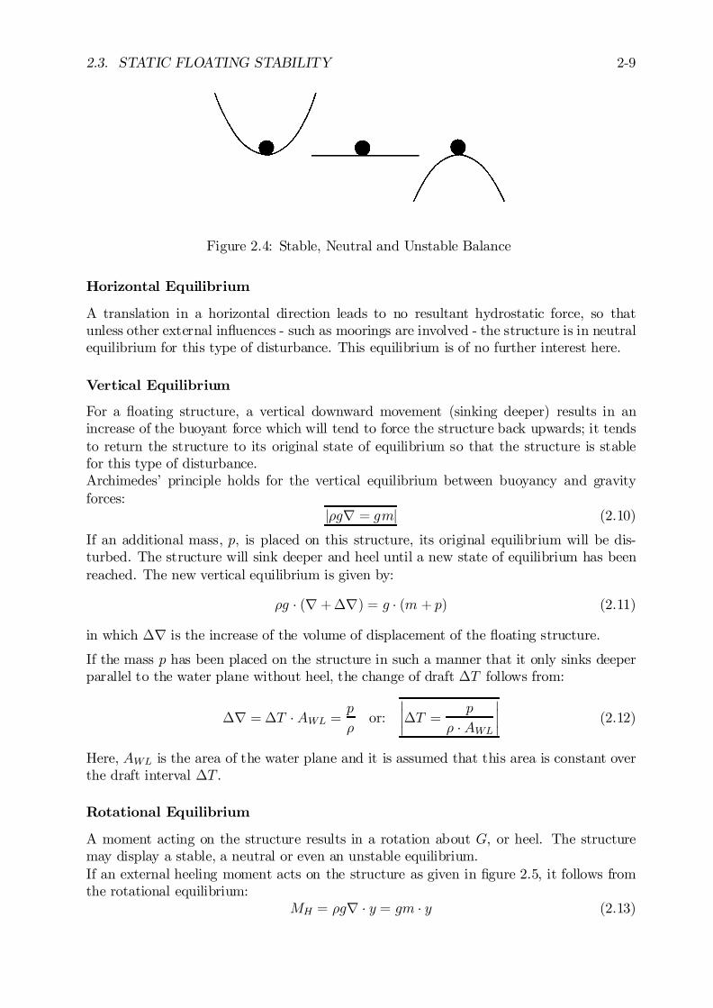
2.3. STATIC FLOATING STABILITY 2-9
Figure 2.4: Stable, Neutral and Unstable Balance
Horizontal Equilibrium
A translation in a horizontal direction leads to no resultant hydrostatic force, so thatunless other external in‡uences - such as moorings are involved - the structure is in neutralequilibrium for this type of disturbance. This equilibrium is of no further interest here.
Vertical Equilibrium
For a ‡oating structure, a vertical downward movement (sinking deeper) results in anincrease of the buoyant force which will tend to force the structure back upwards; it tendsto return the structure to its original state of equilibrium so that the structure is stablefor this type of disturbance.Archimedes’ principle holds for the vertical equilibrium between buoyancy and gravityforces:
j½gr = gmj (2.10)
If an additional mass, p; is placed on this structure, its original equilibrium will be dis-turbed. The structure will sink deeper and heel until a new state of equilibrium has beenreached. The new vertical equilibrium is given by:
½g ¢ (r +¢r) = g ¢ (m + p) (2.11)
in which ¢r is the increase of the volume of displacement of the ‡oating structure.
If the mass p has been placed on the structure in such a manner that it only sinks deeperparallel to the water plane without heel, the change of draft ¢T follows from:
¢r = ¢T ¢ AWL =p
½or:
¯¯¢T = p
½ ¢ AWL
¯¯ (2.12)
Here, AWL is the area of the water plane and it is assumed that this area is constant overthe draft interval ¢T .
Rotational Equilibrium
A moment acting on the structure results in a rotation about G, or heel. The structuremay display a stable, a neutral or even an unstable equilibrium.If an external heeling moment acts on the structure as given in …gure 2.5, it follows fromthe rotational equilibrium:
MH = ½gr ¢ y = gm ¢ y (2.13)
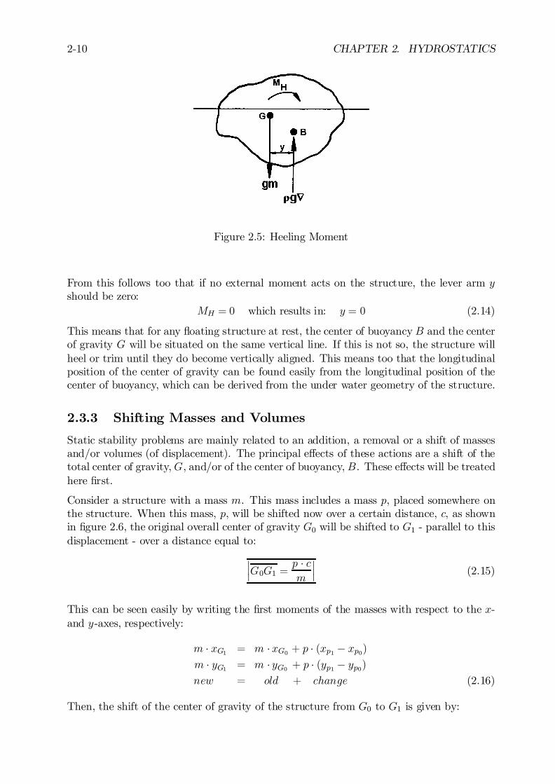
2-10 CHAPTER 2. HYDROSTATICS
Figure 2.5: Heeling Moment
From this follows too that if no external moment acts on the structure, the lever arm yshould be zero:
MH = 0 which results in: y = 0 (2.14)
This means that for any ‡oating structure at rest, the center of buoyancyB and the centerof gravity G will be situated on the same vertical line. If this is not so, the structure willheel or trim until they do become vertically aligned. This means too that the longitudinalposition of the center of gravity can be found easily from the longitudinal position of thecenter of buoyancy, which can be derived from the under water geometry of the structure.
2.3.3 Shifting Masses and Volumes
Static stability problems are mainly related to an addition, a removal or a shift of massesand/or volumes (of displacement). The principal e¤ects of these actions are a shift of thetotal center of gravity,G, and/or of the center of buoyancy,B. These e¤ects will be treatedhere …rst.
Consider a structure with a mass m. This mass includes a mass p, placed somewhere onthe structure. When this mass, p, will be shifted now over a certain distance, c, as shownin …gure 2.6, the original overall center of gravity G0 will be shifted to G1 - parallel to thisdisplacement - over a distance equal to:
¯¯G0G1 =
p ¢ cm
¯¯ (2.15)
This can be seen easily by writing the …rst moments of the masses with respect to the x-and y-axes, respectively:
m ¢ xG1 = m ¢xG0 + p ¢ (xp1 ¡ xp0)m ¢ yG1 = m ¢ yG0 + p ¢ (yp1 ¡ yp0)new = old + change (2.16)
Then, the shift of the center of gravity of the structure from G0 to G1 is given by:
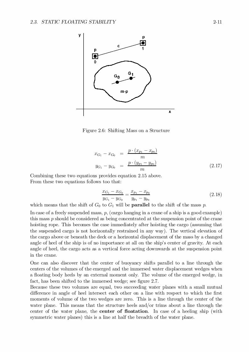
2.3. STATIC FLOATING STABILITY 2-11
Figure 2.6: Shifting Mass on a Structure
xG1 ¡ xG0 =p ¢ (xp1 ¡ xp0)
m
yG1 ¡ yG0 =p ¢ (yp1 ¡ yp0)
m(2.17)
Combining these two equations provides equation 2.15 above.From these two equations follows too that:
xG1 ¡ xG0yG1 ¡ yG0
=xp1 ¡ xp0yp1 ¡ yp0
(2.18)
which means that the shift of G0 to G1 will be parallel to the shift of the mass p.
In case of a freely suspended mass, p, (cargo hanging in a crane of a ship is a good example)this mass p should be considered as being concentrated at the suspension point of the cranehoisting rope. This becomes the case immediately after hoisting the cargo (assuming thatthe suspended cargo is not horizontally restrained in any way). The vertical elevation ofthe cargo above or beneath the deck or a horizontal displacement of the mass by a changedangle of heel of the ship is of no importance at all on the ship’s center of gravity. At eachangle of heel, the cargo acts as a vertical force acting downwards at the suspension pointin the crane.
One can also discover that the center of buoyancy shifts parallel to a line through thecenters of the volumes of the emerged and the immersed water displacement wedges whena ‡oating body heels by an external moment only. The volume of the emerged wedge, infact, has been shifted to the immersed wedge; see …gure 2.7.Because these two volumes are equal, two succeeding water planes with a small mutualdi¤erence in angle of heel intersect each other on a line with respect to which the …rstmoments of volume of the two wedges are zero. This is a line through the center of thewater plane. This means that the structure heels and/or trims about a line through thecenter of the water plane, the center of ‡oatation. In case of a heeling ship (withsymmetric water planes) this is a line at half the breadth of the water plane.
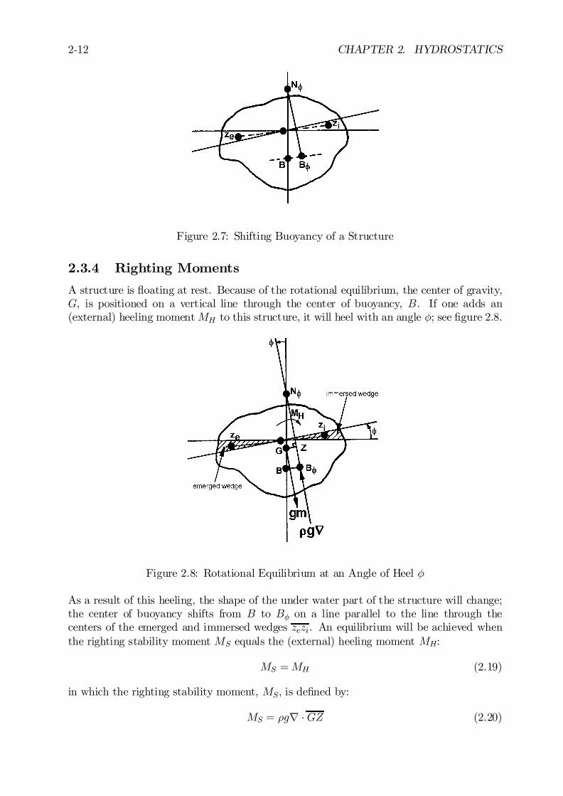
2-12 CHAPTER 2. HYDROSTATICS
Figure 2.7: Shifting Buoyancy of a Structure
2.3.4 Righting Moments
A structure is ‡oating at rest. Because of the rotational equilibrium, the center of gravity,G, is positioned on a vertical line through the center of buoyancy, B. If one adds an(external) heeling momentMH to this structure, it will heel with an angle Á; see …gure 2.8.
Figure 2.8: Rotational Equilibrium at an Angle of Heel Á
As a result of this heeling, the shape of the under water part of the structure will change;the center of buoyancy shifts from B to BÁ on a line parallel to the line through thecenters of the emerged and immersed wedges zezi. An equilibrium will be achieved whenthe righting stability moment MS equals the (external) heeling moment MH:
MS =MH (2.19)
in which the righting stability moment, MS, is de…ned by:
MS = ½gr ¢GZ (2.20)
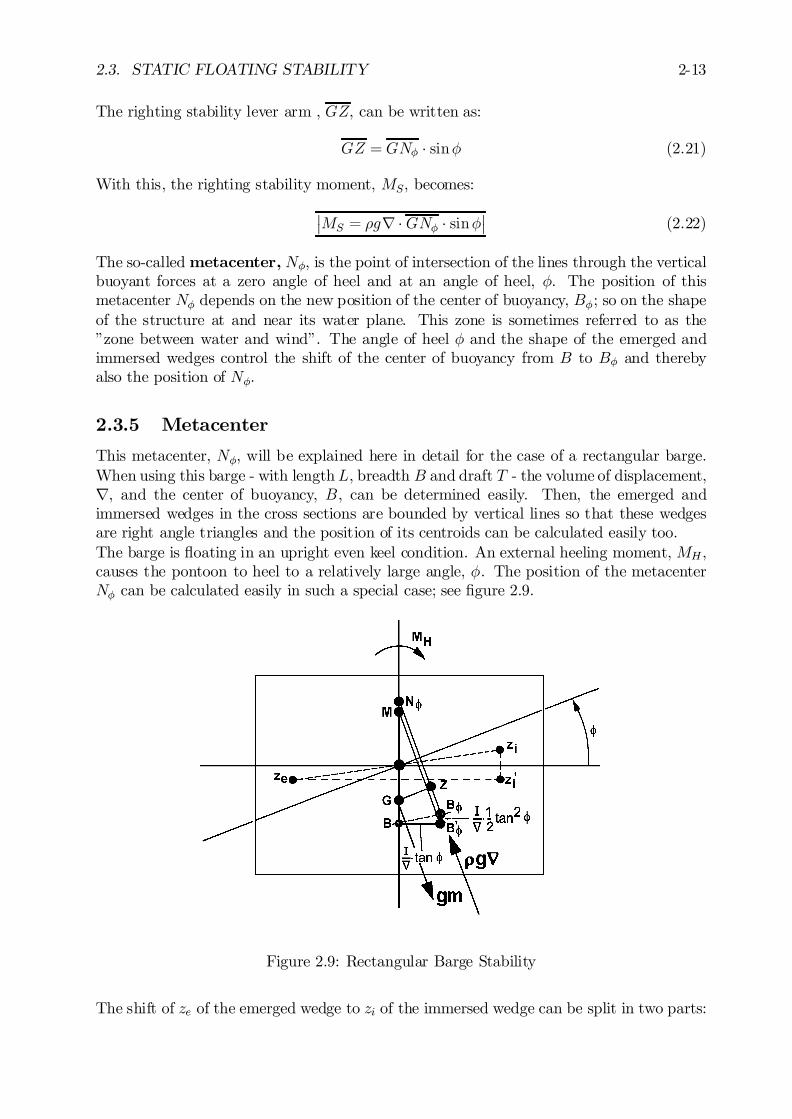
2.3. STATIC FLOATING STABILITY 2-13
The righting stability lever arm , GZ, can be written as:
GZ = GNÁ ¢ sinÁ (2.21)
With this, the righting stability moment, MS, becomes:
¯MS = ½gr ¢GNÁ ¢ sinÁ
¯(2.22)
The so-called metacenter, NÁ, is the point of intersection of the lines through the verticalbuoyant forces at a zero angle of heel and at an angle of heel, Á. The position of thismetacenter NÁ depends on the new position of the center of buoyancy, BÁ; so on the shapeof the structure at and near its water plane. This zone is sometimes referred to as the”zone between water and wind”. The angle of heel Á and the shape of the emerged andimmersed wedges control the shift of the center of buoyancy from B to BÁ and therebyalso the position of NÁ.
2.3.5 Metacenter
This metacenter, NÁ, will be explained here in detail for the case of a rectangular barge.When using this barge - with lengthL, breadth B and draft T - the volume of displacement,r, and the center of buoyancy, B, can be determined easily. Then, the emerged andimmersed wedges in the cross sections are bounded by vertical lines so that these wedgesare right angle triangles and the position of its centroids can be calculated easily too.The barge is ‡oating in an upright even keel condition. An external heeling moment, MH ,causes the pontoon to heel to a relatively large angle, Á. The position of the metacenterNÁ can be calculated easily in such a special case; see …gure 2.9.
Figure 2.9: Rectangular Barge Stability
The shift of ze of the emerged wedge to zi of the immersed wedge can be split in two parts:
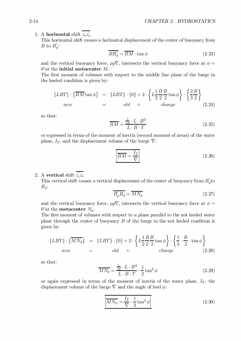
2-14 CHAPTER 2. HYDROSTATICS
1. A horizontal shift zez0i.
This horizontal shift causes a horizontal displacement of the center of buoyancy fromB to B 0
Á:
BB 0Á = BM ¢ tan Á (2.23)
and the vertical buoyancy force, ½gr, intersects the vertical buoyancy force at Á =0±at the initial metacenter M .The …rst moment of volumes with respect to the middle line plane of the barge inthe heeled condition is given by:
fLBTg ¢©BM tan Á
ª= fLBTg ¢ f0g+ 2 ¢
½L1
2
B
2
B
2tanÁ
¾¢½2
3
B
2
¾
new = old + change (2.24)
so that:
BM =112 ¢ L ¢B3L ¢B ¢ T (2.25)
or expressed in terms of the moment of inertia (second moment of areas) of the waterplane, IT , and the displacement volume of the barge r:
¯¯BM =
ITr
¯¯ (2.26)
2. A vertical shift z0izi.This vertical shift causes a vertical displacement of the center of buoyancy from B
0Áto
BÁ:
B0ÁBÁ = MNÁ (2.27)
and the vertical buoyancy force, ½gr, intersects the vertical buoyancy force at Á =0±at the metacenter NÁ.The …rst moment of volumes with respect to a plane parallel to the not heeled waterplane through the center of buoyancy B of the barge in the not heeled condition isgiven by:
fLBT g ¢©MNÁ
ª= fLBT g ¢ f0g+ 2 ¢
½L1
2
B
2
B
2tan Á
¾¢½1
3¢ B2
¢ tanÁ¾
new = old + change (2.28)
so that:
MNÁ =112
¢ L ¢B3L ¢B ¢ T ¢ 1
2tan2 Á (2.29)
or again expressed in terms of the moment of inertia of the water plane, IT , thedisplacement volume of the barge r and the angle of heel Á:
¯¯MNÁ =
ITr ¢ 1
2tan2 Á
¯¯ (2.30)

2.3. STATIC FLOATING STABILITY 2-15
Now the position of the metacenter NÁ follows from a superposition of equations 2.26 and2.30:
BNÁ = BM +MNÁ
=ITr ¢
µ1 +
1
2tan2 Á
¶(2.31)
or: ¯¯BNÁ = BM ¢
µ1 +
1
2tan2 Á
¶¯¯ (2.32)
The term BM ¢ 1 represents the e¤ect of the horizontal part of the shift of ze to zi andthe term BM ¢ 1
2tan2 Á represents the e¤ect of the vertical part of this shift. Note that the
angle of heel, Á, has no e¤ect on M ; but it has e¤ect on NÁ.
2.3.6 Scribanti Formula
Figure 2.10: Wall Sided Structure
A ‡oating structure is said to be wall-sided if, for the angles of heel to be considered,those portions of the hull covered or uncovered by the changing water plane are verticalwhen the structure is ‡oating upright; see …gure 2.10. The wedges in the cross sections arebounded by vertical lines - as is the case for the barge - so that the emerged and immersedwedges are right angle symmetrical triangles and the position of the metacenter NÁ can becalculated easily in such a special case.It can be found that - regardless the under-water geometry of a structure - equation 2.30is valid for all wall-sided structures:
¯¯BNÁ =
ITr ¢ (1 + 1
2tan2 Á)
¯¯ Scribanti Formula (2.33)

2-16 CHAPTER 2. HYDROSTATICS
in which IT is the transverse moment of inertia (second moment of areas) of the not heeledwater plane about the axis of inclination for both half water planes.This is a fairly good approximation for ships that have vertical sides over a great part ofthe length and which are not so far heeled that the deck enters the water or the bottomcomes above the water level.
At small angles of heel (up to about 10 degrees), the e¤ect of the vertical shift of thecenter of buoyancy, B 0
ÁBÁ = MNÁ, can be ignored. This can be seen in the Scribantiformula too, because in that case 1
2tan2 Á is very small compared to 1.0. The work line
of the vertical buoyancy force, ½gr, intersects the work line of the vertical buoyancy forcefor Á = 0± at the initial metacenter, M, which location is de…ned by equation 2.26, usefulfor Á < §10±. Up to angles of heel of about 10 degrees, this is a fairly good approximationof the metacenter of the ships that are almost wall-sided at the ”zone between water andwind” over a relatively large part of the length. Sailing yachts for instance, do not ful…lthis requirement.
At larger angles of heel, the e¤ect of the vertical shift of the center of buoyancy mustbe taken into account. The work line of the vertical buoyancy force, ½gr, intersects thework line of the vertical buoyancy force for Á = 0± at the metacenter,NÁ, which locationis de…ned by equation 2.32, useful for Á > §10±. Use of this formula yields su¢cientlyaccurate results for ”non-Scribanti” ships until heel angles of heel of about 20 to 25 degrees.Keep in mind that this formula is not longer valid when the angle of heel gets so large thatthe water plane changes rapidly. This is the case when the bilge or chine (the ”corner”where the sides of a ship meet its bottom) comes out of the water or the deck enters thewater, for example. This possibility always has to be checked, when carrying out stabilitycalculations!
It has been shown above that the metacenter is de…ned by the intersection of lines throughthe vertical buoyant forces at a heel angle Á and a heel angle Á + ¢Á. Depending onthe magnitude of Á and the increment ¢Á, two di¤erent metacenter de…nitions have beendistinguished here, as tabled below.
metacenter point symbol Á ¢Á
initial metacenter M 0 very smallmetacenter NÁ 0 larger
Note that - for symmetrical under water forms like ships - both the metacenters M andNÁ are situated in the middle line plane (Á = 0).
The stability lever armGZ = GNÁ ¢sinÁ is determined by the hydrostatic properties of thesubmerged structure (form and heel dependent) and the position of the center of gravityof this structure (mass distribution dependent). This is the reason why the followingexpression for GNÁ has been introduced:
¯GNÁ =KB + BNÁ ¡KG
¯(2.34)
Here, K is the keel point of the structure; see …gure 2.10.The magnitude of KB follows from the under water geometry of the structure and themagnitude of KG follows from the mass distribution of the structure.
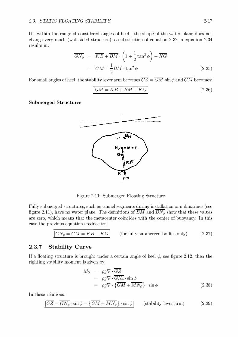
2.3. STATIC FLOATING STABILITY 2-17
If - within the range of considered angles of heel - the shape of the water plane does notchange very much (wall-sided structure), a substitution of equation 2.32 in equation 2.34results in:
GNÁ = KB + BM ¢µ1 +
1
2tan2 Á
¶¡KG
= GM +1
2BM ¢ tan2 Á (2.35)
For small angles of heel, the stability lever arm becomesGZ = GM ¢sinÁ andGM becomes:¯GM =KB + BM ¡KG
¯(2.36)
Submerged Structures
Figure 2.11: Submerged Floating Structure
Fully submerged structures, such as tunnel segments during installation or submarines (see…gure 2.11), have no water plane. The de…nitions of BM and BNÁ show that these valuesare zero, which means that the metacenter coincides with the center of buoyancy. In thiscase the previous equations reduce to:
¯GNÁ = GM = KB ¡KG
¯(for fully submerged bodies only) (2.37)
2.3.7 Stability Curve
If a ‡oating structure is brought under a certain angle of heel Á, see …gure 2.12, then therighting stability moment is given by:
MS = ½gr ¢GZ= ½gr ¢GNÁ ¢ sinÁ= ½gr ¢
©GM +MNÁ
ª¢ sinÁ (2.38)
In these relations:¯GZ = GNÁ ¢ sinÁ =
©GM +MNÁ
ª¢ sinÁ
¯(stability lever arm) (2.39)
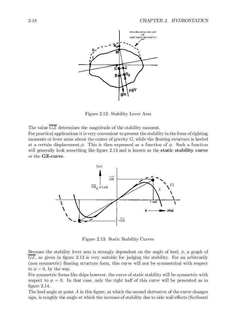
2-18 CHAPTER 2. HYDROSTATICS
Figure 2.12: Stability Lever Arm
The value GZ determines the magnitude of the stability moment.For practical applications it is very convenient to present the stability in the form of rightingmoments or lever arms about the center of gravity G, while the ‡oating structure is heeledat a certain displacement,Á. This is then expressed as a function of Á. Such a functionwill generally look something like …gure 2.13 and is known as the static stability curveor the GZ-curve.
Figure 2.13: Static Stability Curves
Because the stability lever arm is strongly dependent on the angle of heel, Á, a graph ofGZ, as given in …gure 2.13 is very suitable for judging the stability. For an arbitrarily(non symmetric) ‡oating structure form, this curve will not be symmetrical with respectto Á = 0, by the way.For symmetric forms like ships however, the curve of static stability will be symmetric withrespect to Á = 0. In that case, only the right half of this curve will be presented as in…gure 2.14.The heel angle at point A in this …gure, at which the second derivative of the curve changessign, is roughly the angle at which the increase of stability due to side wall e¤ects (Scribanti

2.3. STATIC FLOATING STABILITY 2-19
Figure 2.14: Ship Static Stability Curve
formula) starts to be counteracted by the fact that the deck enters the water or the bilgecomes above the water.
Figure 2.15 shows the static stability curve when the initial metacentric height, GM , isnegative while GZ becomes positive at some reasonable angle of heel Á1, the so-calledangle of loll.
Figure 2.15: Static Stability Curve with a Negative GM
If the ‡oating structure is momentarily at some angle of heel less than Á1, the momentacting on the structure due to GZ tends to increase the heel. If the angle is greater than Á1,the moment tends to reduce the heel. Thus the angle Á1 is a position of stable equilibrium.Unfortunately, since the GZ curve is symmetrical about the origin, as Á1 is decreased, the‡oating structure eventually passes through the upright condition and will then suddenlylurch over towards the angle ¡Á1 on the opposite side and overshoot this value (because ofdynamic e¤ects) before reaching a steady state. This causes an unpleasant rolling motion,which is often the only direct indication that the heel to one side is due to a negative GMrather than a positive heeling moment acting on the structure.

2-20 CHAPTER 2. HYDROSTATICS
Characteristics of Stability Curve
Some important characteristics of the static stability curve can be summarized here:
1. Slope at The OriginFor small angles of heel, the righting lever arm is proportional to the curve slope andthe metacenter is e¤ectively a …xed point. It follows, that the tangent to the GZcurve at the origin represents the metacentric height GM . This can be shown easilyfor the case of a wall-sided structure:
d
dÁ
©GZ
ª=
d
dÁ
©GNÁ ¢ sinÁ
ª
=d
dÁ
½µGM +
1
2BM ¢ tan2 Á
¶¢ sinÁ
¾(2.40)
This derivative becomes GM for zero heel. This means that the initial metacentricheight GM can be of great importance for the further form of the curve, especiallyat smaller angles of heel, and for the area under the curve (see item 5 below).
2. Maximum GZ ValueThe maximum GZ value is rules the largest steady heeling moment that the ‡oatingstructure can resist without capsizing. Its value and the angle at which it occurs areboth important. The shape of the above-water part of the ‡oating structure is ofgreat importance for the maximum attainable value of the stability lever arm.
3. Range of StabilityAt some angle of heel (sometimes even greater than 90 degrees) the GZ value de-creases again to zero and even becomes negative for larger inclinations. This angleis known as the angle of vanishing stability. The range of angles for which GZis positive is known as the range of stability. This range is of great importancefor the maximum attainable area under the stability curve and thereby also on themaximum potential energy that the structure can absorb via a roll motion. Theshape of the above-water part has a large in‡uence on the angle of vanishing stabil-ity; compare curves I and II in …gures 2.12 and 2.13. For angles within the rangeof stability, a ‡oating structure will return to the upright state when the heelingmoment is removed.
4. Angle of Deck Edge ImmersionFor most ‡oating structures, there is a point of in‡ection in the stability curve,corresponding roughly to the angle at which the deck edge becomes immersed. Thispoint is not so much of interest in its own right as in the fact that it provides guidanceto the designer upon the possible e¤ect of certain design changes on stability. Theshape of the above water part of the structure can have a large in‡uence on its staticstability. More or less the same statement can be made when the bilge or the bottomchine emerges, because of the decrease of the breadth of the water line. Keep in mindthat for wall-sided structures, when the deck enters the water or the bottom chinecomes above the water level, the immersed and emerged wedges are no longer nicetriangles; calculations become much more cumbersome!
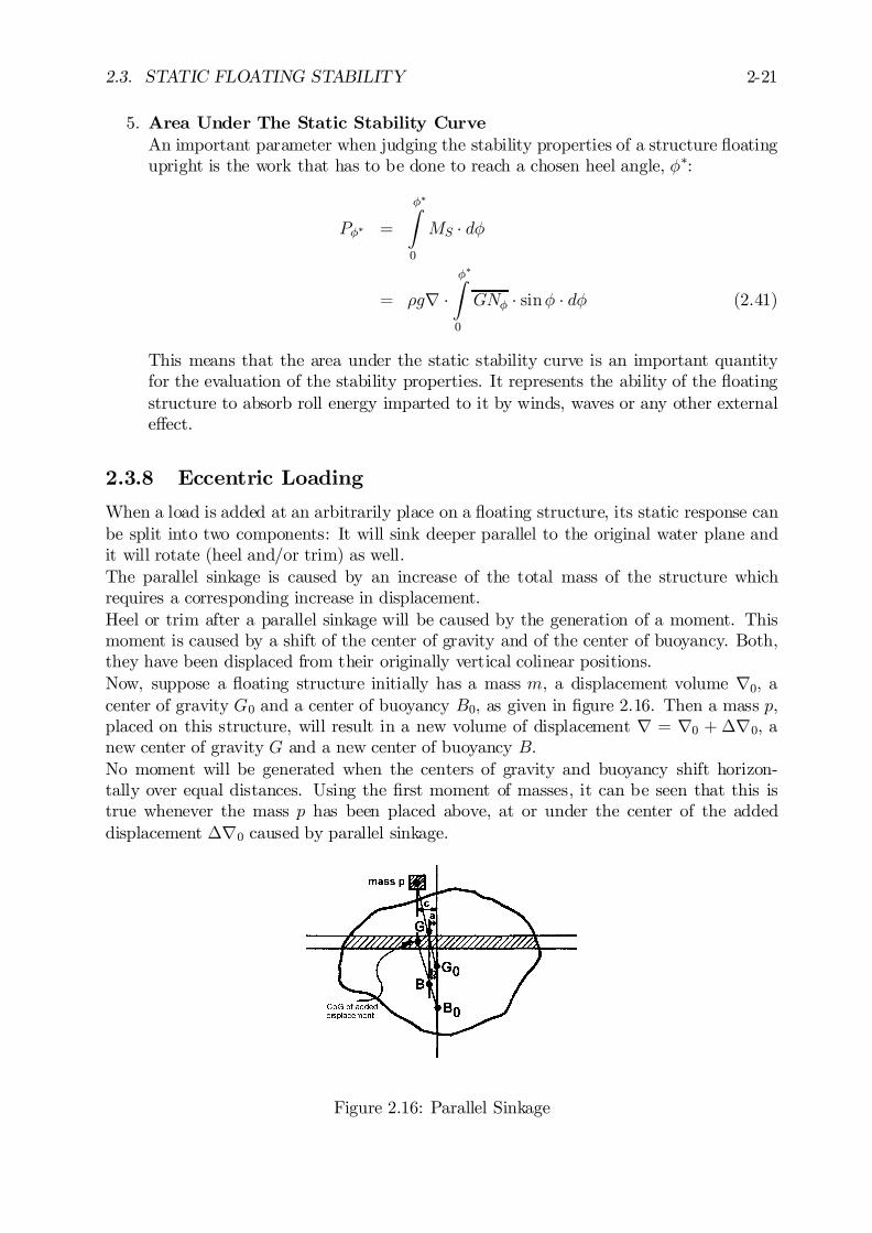
2.3. STATIC FLOATING STABILITY 2-21
5. Area Under The Static Stability CurveAn important parameter when judging the stability properties of a structure ‡oatingupright is the work that has to be done to reach a chosen heel angle, Á¤:
PÁ¤ =
Á¤Z
0
MS ¢ dÁ
= ½gr ¢Á¤Z
0
GNÁ ¢ sinÁ ¢ dÁ (2.41)
This means that the area under the static stability curve is an important quantityfor the evaluation of the stability properties. It represents the ability of the ‡oatingstructure to absorb roll energy imparted to it by winds, waves or any other externale¤ect.
2.3.8 Eccentric Loading
When a load is added at an arbitrarily place on a ‡oating structure, its static response canbe split into two components: It will sink deeper parallel to the original water plane andit will rotate (heel and/or trim) as well.The parallel sinkage is caused by an increase of the total mass of the structure whichrequires a corresponding increase in displacement.Heel or trim after a parallel sinkage will be caused by the generation of a moment. Thismoment is caused by a shift of the center of gravity and of the center of buoyancy. Both,they have been displaced from their originally vertical colinear positions.Now, suppose a ‡oating structure initially has a mass m, a displacement volume r0, acenter of gravity G0 and a center of buoyancy B0, as given in …gure 2.16. Then a mass p,placed on this structure, will result in a new volume of displacement r = r0 + ¢r0, anew center of gravity G and a new center of buoyancy B.No moment will be generated when the centers of gravity and buoyancy shift horizon-tally over equal distances. Using the …rst moment of masses, it can be seen that this istrue whenever the mass p has been placed above, at or under the center of the addeddisplacement ¢r0 caused by parallel sinkage.
Figure 2.16: Parallel Sinkage
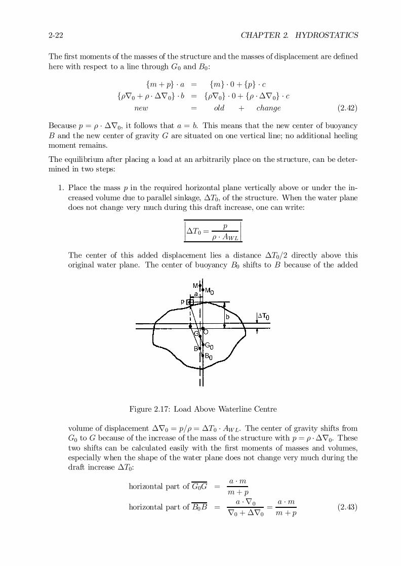
2-22 CHAPTER 2. HYDROSTATICS
The …rst moments of the masses of the structure and the masses of displacement are de…nedhere with respect to a line through G0 and B0:
fm+ pg ¢ a = fmg ¢ 0 + fpg ¢ cf½r0 + ½ ¢¢r0g ¢ b = f½r0g ¢ 0 + f½ ¢¢r0g ¢ c
new = old + change (2.42)
Because p = ½ ¢ ¢r0, it follows that a = b. This means that the new center of buoyancyB and the new center of gravity G are situated on one vertical line; no additional heelingmoment remains.
The equilibrium after placing a load at an arbitrarily place on the structure, can be deter-mined in two steps:
1. Place the mass p in the required horizontal plane vertically above or under the in-creased volume due to parallel sinkage, ¢T0; of the structure. When the water planedoes not change very much during this draft increase, one can write:
¯¯¢T0 =
p
½ ¢ AWL
¯¯
The center of this added displacement lies a distance ¢T0=2 directly above thisoriginal water plane. The center of buoyancy B0 shifts to B because of the added
Figure 2.17: Load Above Waterline Centre
volume of displacement ¢r0 = p=½ = ¢T0 ¢ AWL. The center of gravity shifts fromG0 to G because of the increase of the mass of the structure with p = ½ ¢¢r0. Thesetwo shifts can be calculated easily with the …rst moments of masses and volumes,especially when the shape of the water plane does not change very much during thedraft increase ¢T0:
horizontal part of G0G =a ¢mm+ p
horizontal part of B0B =a ¢r0
r0 + ¢r0=a ¢mm + p
(2.43)
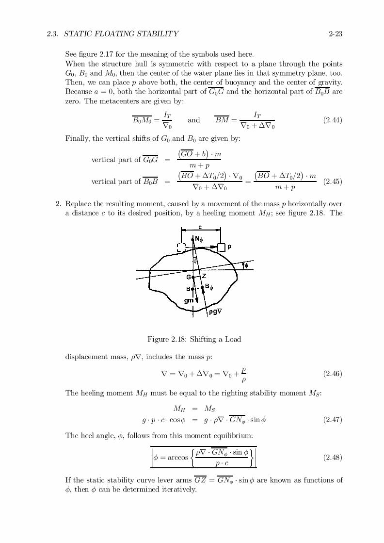
2.3. STATIC FLOATING STABILITY 2-23
See …gure 2.17 for the meaning of the symbols used here.When the structure hull is symmetric with respect to a plane through the pointsG0, B0 and M0, then the center of the water plane lies in that symmetry plane, too.Then, we can place p above both, the center of buoyancy and the center of gravity.Because a = 0, both the horizontal part of G0G and the horizontal part of B0B arezero. The metacenters are given by:
B0M0 =ITr0
and BM =IT
r0 +¢r0(2.44)
Finally, the vertical shifts of G0 and B0 are given by:
vertical part of G0G =
¡GO + b
¢¢m
m+ p
vertical part of B0B =
¡BO +¢T0=2
¢¢ r0
r0 + ¢r0=
¡BO + ¢T0=2
¢¢m
m+ p(2.45)
2. Replace the resulting moment, caused by a movement of the mass p horizontally overa distance c to its desired position, by a heeling moment MH ; see …gure 2.18. The
Figure 2.18: Shifting a Load
displacement mass, ½r; includes the mass p:
r = r0 +¢r0 = r0 +p
½(2.46)
The heeling moment MH must be equal to the righting stability moment MS:
MH = MS
g ¢ p ¢ c ¢ cosÁ = g ¢ ½r ¢GNÁ ¢ sinÁ (2.47)
The heel angle, Á; follows from this moment equilibrium:¯¯Á = arccos
½½r ¢GNÁ ¢ sin Á
p ¢ c
¾¯¯ (2.48)
If the static stability curve lever arms GZ = GNÁ ¢ sinÁ are known as functions ofÁ, then Á can be determined iteratively.

2-24 CHAPTER 2. HYDROSTATICS
For wall-sided structures one can substitute equation 2.35 in equation 2.48 andget: ¯
¯¯Á = arccos
(½r ¢
©GM + 1
2BM ¢ tan2 Á
ª¢ sinÁ
p ¢ c
)¯¯¯ (2.49)
or using tanÁ: ¯¯12BM ¢ tan3 Á+ GM ¢ tan Á = p ¢ c
½r
¯¯ (2.50)
This third degree equation in tanÁ can be solved iteratively using the Regula-Falsimethod by calculating the Left Hand Side (LHS) of the equation as a function of Áuntil a value equal to the value of the Right Hand Side (RHS) has been found.For small angles of heel and when the shape of the water plane does not change verymuch, the expression for Á can be simpli…ed to become:
¯¯Á = arctan
½p ¢ c
½r ¢GM
¾¯¯ (2.51)
so that Á can be found directly in this situation.
2.3.9 Inclining Experiment
Much of the data used in stability calculations depends only on the geometry of the struc-ture. The total mass of the structure m follows from the displacement volume, r. Thelongitudinal position of the center of gravity, G; follows simply from the longitudinal posi-tion of the center of buoyancy, B, which can be determined from the under water geometryof the structure. The vertical position of the center of gravity must be known before thestability can be completely assessed for a given loading condition. Since the vertical po-sition of the center of gravity, KG, sometimes can be 10 times greater than the initialmetacentric height GM , KG must be known very accurately if the metacentric height isto be assessed with reasonable accuracy. KG can be calculated for a variety of loadingconditions, provided it is accurately known for one precisely speci…ed loading condition.The displacement volume, r can be calculated, given the geometry of the structure, incombination with measured drafts fore and aft (at both ends) in the upright condition(Á = Á0 ¼ 0±). With this displacement and the measured angle of heel (Á = Á1) aftershifting a known mass p on the structure over a distance c, the vertical position of thecenter of gravity can be found easily by writing equation 2.51 in another form:
¯¯GM =
p ¢ c½r ¢ tan (Á1¡ Á0)
¯¯ with: Á0 ¿ Á1 and Á1 < §10± (2.52)
The known underwater geometry of the structure and this ”measured” GM value yieldsthe vertical position of the center of gravity G.
An experiment to determine the metacentric height in this way is called an incliningexperiment. The purposes of this experiment are to determine the displacement, r;and the position of the center of gravity of the structure under a precisely known set ofconditions. It is usually carried out when construction is being completed (a‡oat) beforeleaving the construction yard. An additional inclining experiment may be carried outfollowing an extensive modernization or a major re…t. Keep in mind that r and G haveto be corrected when the mass p is removed from the structure, again.

2.3. STATIC FLOATING STABILITY 2-25
2.3.10 Free Surface Correction
Free surfaces of liquids inside a ‡oating structure can have a large in‡uence on its staticstability; they reduce the righting moment or stability lever arm.
Figure 2.19: Floating Structure with a Tank Partially Filled with Liquid
When the structure in …gure 2.19 heels as a result of an external moment MH , the surfaceof the ‡uid in the tank remains horizontal. This means that this free surface heels relativeto the structure itself, so that the center of gravity of the structure (including liquid) shifts.This shift is analogous to the principle of the shift of the center of buoyancy due to theemerged and immersed wedges, as discussed above. Of course, the under water geometryof the entire structure and the boundaries of the wedges at the water plane as well as in thetank play a role. They determine, together with the angle of heel, the amount by whichthe centers of buoyancy and of gravity now shift.In case of a vertical wedge boundary, (a wall-sided tank) as given in …gure 2.20, this shiftcan be calculated easily with the …rst moment of volumes with triangular cross sections.In this …gure, ½0 is the density of the liquid in the tank, v is the volume of the liquid in the
Figure 2.20: E¤ect of a Liquid Free Surface in a Wall Sided Tank
tank and i is the transverse moment of inertia (second moment of areas) of the surface of
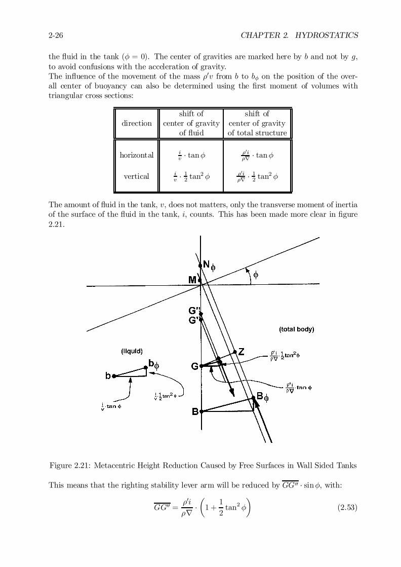
2-26 CHAPTER 2. HYDROSTATICS
the ‡uid in the tank (Á = 0). The center of gravities are marked here by b and not by g,to avoid confusions with the acceleration of gravity.The in‡uence of the movement of the mass ½0v from b to bÁ on the position of the over-all center of buoyancy can also be determined using the …rst moment of volumes withtriangular cross sections:
shift of shift ofdirection center of gravity center of gravity
of ‡uid of total structure
horizontal iv ¢ tanÁ ½0i
½r ¢ tanÁ
vertical iv ¢ 12 tan2 Á ½0i
½r ¢ 12 tan2 Á
The amount of ‡uid in the tank, v, does not matters, only the transverse moment of inertiaof the surface of the ‡uid in the tank, i, counts. This has been made more clear in …gure2.21.
Figure 2.21: Metacentric Height Reduction Caused by Free Surfaces in Wall Sided Tanks
This means that the righting stability lever arm will be reduced by GG00 ¢ sinÁ, with:
GG00 =½0i½r ¢
µ1 +
1
2tan2 Á
¶(2.53)

2.3. STATIC FLOATING STABILITY 2-27
The magnitude GG00 is called the free surface correction or the reduction of themetacentric height.For small angles of heel for which 1
2tan2 Á is small relative to 1:0, one can write for the
reduction of the metacentric height:
GG00 ¼ GG0 =½0i½r (2.54)
For more free surfaces (more tanks) the reduction of the metacentric height becomes:
¯¯GG00 =
Pf½0ig½r ¢
µ1 +
1
2tan2 Á
¶¯¯ (2.55)
Figure 2.22: GZ-Curve, Corrected for Free Surface
Note that the e¤ect of the free surface on the stability lever arm (see …gure 2.22) is inde-pendent of the position of the tank in the ‡oating structure; the tank can be at any heightin the structure and at any position in its length or breadth.The e¤ect is also independent of the amount of liquid in the tank, provided that the momentof inertia (second moment of areas) of the free surface remains substantially unchangedwhen inclined. The moment of inertia of the free surface of a tank which is almost emptyor almost full can change signi…cantly during an inclining experiment. This is why tankswhich cannot be completely full or empty during an inclining experiment are speci…ed tobe half full.It is common practice to treat the free surface e¤ect as being equivalent to a virtual riseof the center of gravity of the structure. One should appreciate that this is merely aconvention which has no factual basis in reality.A similar free surface e¤ect can arise from movements of granular cargo such as grainwhich is stowed in bulk. Here, however, there is no simple relation between the angle ofinclination of the ship and the slope of the surface of the grain. At small angles of heelthe grain is not likely to shift, so there is no in‡uence on initial stability. When the heel

2-28 CHAPTER 2. HYDROSTATICS
angle becomes great enough, a signi…cant shift can take place very abruptly; its e¤ect canbe equally abrupt!

2.3. STATIC FLOATING STABILITY 2-29
.

2-30 CHAPTER 2. HYDROSTATICS

Chapter 3
CONSTANT POTENTIAL FLOWPHENOMENA
3.1 Introduction
This chapter introduces hydrodynamics by treating the simplest of ‡ows: constant, in-compressible, potential ‡ows; time is therefore unimportant. These ‡ows obey reasonablysimpli…ed laws of ‡uid mechanics and mathematics as will be explained in this chapter. Inspite of its limitations, potential ‡ow is widely used in ‡uid mechanics. It often gives atleast a qualitative impression of ‡ow phenomena. Discrepancies between real and idealized‡ows are often accommodated via experimentally determined coe¢cients.The concepts introduced in this chapter will be extended and applied in later chapters fora wide variety of solutions including those involving waves. Indeed, potential theory canvery easily be extended to time dependent ‡ows as well. This chapter starts by de…ninga potential ‡ow …eld and its properties in a very general way. The power of the methodwill become more obvious as it is applied to constant ‡ow situations later in this chapter.Much of the information in this chapter may be well-known to the reader; it can be seenas a quick review. In any case, this chapter introduces the notation used in many of theremaining chapters as well.
3.2 Basis Flow Properties
All ‡ows are treated here as being non-viscous, incompressible, continuous andhomogeneous. There are no cavitation holes or gas bubbles in the ‡uid.
3.2.1 Continuity Condition
Consider …rst a di¤erential element of ‡uid within a larger body of a compressible ‡ow.This block has edges with dimensions dx by dy by dz oriented parallel to the axes of aright-handed (x; y; z)-axis system as shown in …gure 3.1 (only the y-component of velocityis shown).
0J.M.J. Journée and W.W. Massie, ”OFFSHORE HYDROMECHANICS”, First Edition, January 2001,Delft University of Technology. For updates see web site: http://www.shipmotions.nl.
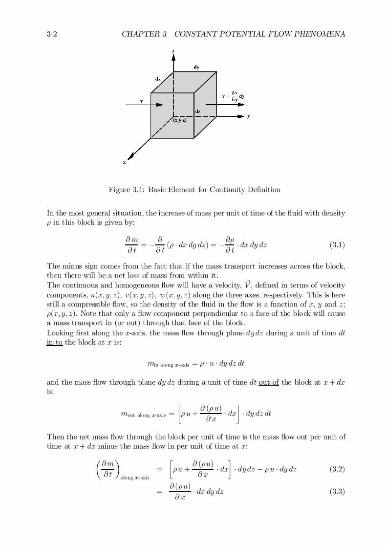
3-2 CHAPTER 3. CONSTANT POTENTIAL FLOW PHENOMENA
Figure 3.1: Basic Element for Continuity De…nition
In the most general situation, the increase of mass per unit of time of the ‡uid with density½ in this block is given by:
@ m
@ t= ¡ @
@ t(½ ¢ dx dy dz) = ¡@½
@ t¢ dx dy dz (3.1)
The minus sign comes from the fact that if the mass transport increases across the block,then there will be a net loss of mass from within it.The continuous and homogeneous ‡ow will have a velocity, ~V , de…ned in terms of velocitycomponents, u(x; y; z); v(x; y; z); w(x; y; z) along the three axes, respectively. This is herestill a compressible ‡ow, so the density of the ‡uid in the ‡ow is a function of x, y and z;½(x; y; z): Note that only a ‡ow component perpendicular to a face of the block will causea mass transport in (or out) through that face of the block.Looking …rst along the x-axis, the mass ‡ow through plane dydz during a unit of time dtin-to the block at x is:
min along x-axis = ½ ¢ u ¢ dy dz dt
and the mass ‡ow through plane dy dz during a unit of time dt out-of the block at x+ dxis:
mout along x-axis =
·½ u+
@ (½ u)
@ x¢ dx
¸¢ dy dz dt
Then the net mass ‡ow through the block per unit of time is the mass ‡ow out per unit oftime at x+ dx minus the mass ‡ow in per unit of time at x:
µ@m
@ t
¶
along x-axis
=
·½u +
@ (½u)
@ x¢ dx
¸¢ dydz ¡ ½ u ¢ dy dz (3.2)
=@ (½u)
@ x¢ dx dy dz (3.3)
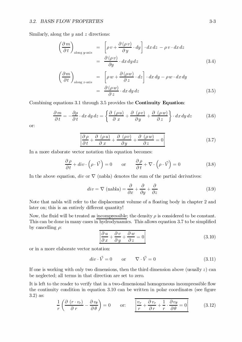
3.2. BASIS FLOW PROPERTIES 3-3
Similarly, along the y and z directions:µ@ m
@ t
¶
along y-axis
=
·½ v+
@ (½ v)
@ y¢ dy
¸¢ dxdz ¡ ½ v ¢ dxdz
=@ (½ v)
@y¢ dxdydz (3.4)
µ@m
@ t
¶
along z-axis
=
·½ w +
@ (½w)
@ z¢ dz
¸¢ dx dy ¡ ½w ¢ dxdy
=@ (½ w)
@ z¢ dx dy dz (3.5)
Combining equations 3.1 through 3.5 provides the Continuity Equation:
@ m
@ t= ¡@½
@ t¢ dx dy dz =
½@ (½u)
@ x+@ (½v)
@ y+@ (½ w)
@ z
¾¢ dxdy dz (3.6)
or:
¯¯@ ½@ t+@ (½ u)
@ x+@ (½v)
@ y+@ (½ w)
@ z= 0
¯¯ (3.7)
In a more elaborate vector notation this equation becomes:
@ ½
@ t+ div ¢
³½ ¢ ~V
´= 0 or
@ ½
@ t+r ¢
³½ ¢ ~V
´= 0 (3.8)
In the above equation, div or r (nabla) denotes the sum of the partial derivatives:
div = r (nabla) =@
@x+@
@y+@
@z(3.9)
Note that nabla will refer to the displacement volume of a ‡oating body in chapter 2 andlater on; this is an entirely di¤erent quantity!
Now, the ‡uid will be treated as incompressible; the density ½ is considered to be constant.This can be done in many cases in hydrodynamics. This allows equation 3.7 to be simpli…edby cancelling ½: ¯
¯@ u@ x
+@ v
@ y+@ w
@ z= 0
¯¯ (3.10)
or in a more elaborate vector notation:
div ¢ ~V = 0 or r ¢ ~V = 0 (3.11)
If one is working with only two dimensions, then the third dimension above (usually z) canbe neglected; all terms in that direction are set to zero.
It is left to the reader to verify that in a two-dimensional homogeneous incompressible ‡owthe continuity condition in equation 3.10 can be written in polar coordinates (see …gure3.2) as:
1
r
µ@ (r ¢ vr)@ r
¡ @ vµ@ µ
¶= 0 or:
¯¯vrr+@ vr@ r
+1
r¢ @ vµ@ µ
= 0
¯¯ (3.12)
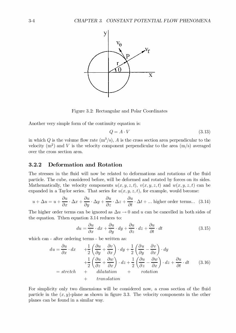
3-4 CHAPTER 3. CONSTANT POTENTIAL FLOW PHENOMENA
Figure 3.2: Rectangular and Polar Coordinates
Another very simple form of the continuity equation is:
Q= A ¢ V (3.13)
in which Q is the volume ‡ow rate (m3/s), A is the cross section area perpendicular to thevelocity (m2) and V is the velocity component perpendicular to the area (m/s) averagedover the cross section area.
3.2.2 Deformation and Rotation
The stresses in the ‡uid will now be related to deformations and rotations of the ‡uidparticle. The cube, considered before, will be deformed and rotated by forces on its sides.Mathematically, the velocity components u(x; y; z; t), v(x; y; z; t) and w(x; y; z; t) can beexpanded in a Taylor series. That series for u(x; y; z; t), for example, would become:
u+ ¢u = u+@u
@x¢¢x + @u
@y¢¢y + @u
@z¢¢z + @u
@t¢¢t+ ::: higher order terms::: (3.14)
The higher order terms can be ignored as ¢u! 0 and u can be cancelled in both sides ofthe equation. Tthen equation 3.14 reduces to:
du =@u
@x¢ dx + @u
@y¢ dy + @u
@z¢ dz + @u
@t¢ dt (3.15)
which can - after ordering terms - be written as:
du =@u
@x¢ dx +
1
2
µ@u
@y+@v
@x
¶¢ dy + 1
2
µ@u
@y¡ @v
@x
¶¢ dy
+1
2
µ@u
@z+@w
@x
¶¢ dz + 1
2
µ@u
@z¡ @w
@x
¶¢ dz + @u
@t¢ dt (3.16)
= stretch + dilatation + rotation
+ translation
For simplicity only two dimensions will be considered now, a cross section of the ‡uidparticle in the (x; y)-plane as shown in …gure 3.3. The velocity components in the otherplanes can be found in a similar way.
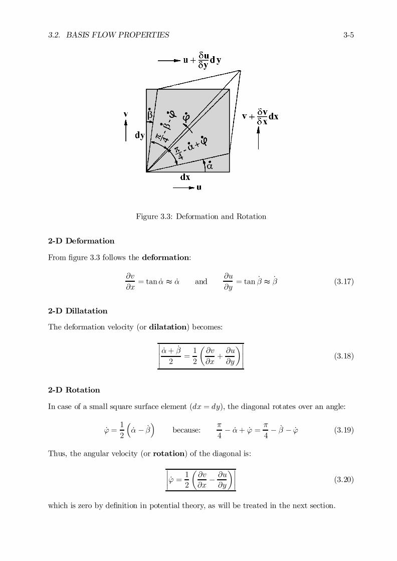
3.2. BASIS FLOW PROPERTIES 3-5
Figure 3.3: Deformation and Rotation
2-D Deformation
From …gure 3.3 follows the deformation:
@v
@x= tan _® t _® and
@u
@y= tan _ t _ (3.17)
2-D Dillatation
The deformation velocity (or dilatation) becomes:
¯¯¯_®+ _
2=1
2
µ@v
@x+@u
@y
¶¯¯¯ (3.18)
2-D Rotation
In case of a small square surface element (dx = dy), the diagonal rotates over an angle:
_' =1
2
³_® ¡ _
´because:
¼
4¡ _®+ _' =
¼
4¡ _ ¡ _' (3.19)
Thus, the angular velocity (or rotation) of the diagonal is:
¯¯ _' = 1
2
µ@v
@x¡ @u
@y
¶¯¯ (3.20)
which is zero by de…nition in potential theory, as will be treated in the next section.
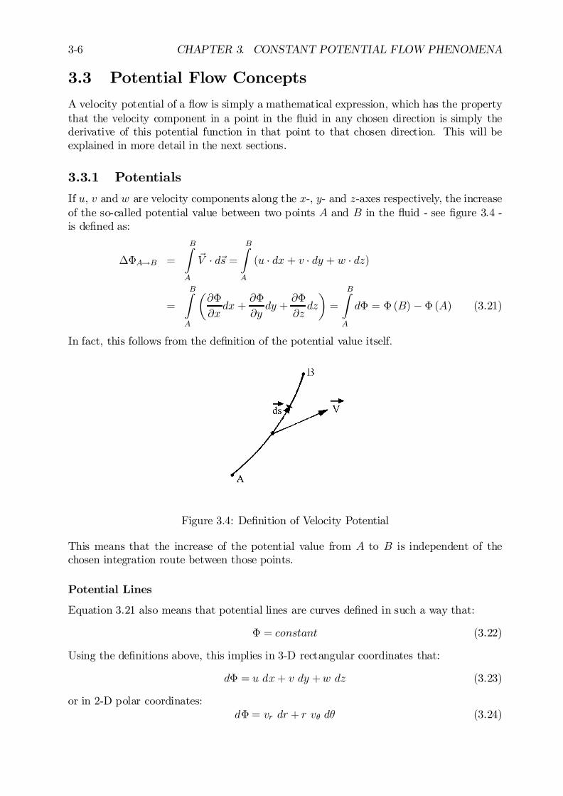
3-6 CHAPTER 3. CONSTANT POTENTIAL FLOW PHENOMENA
3.3 Potential Flow Concepts
A velocity potential of a ‡ow is simply a mathematical expression, which has the propertythat the velocity component in a point in the ‡uid in any chosen direction is simply thederivative of this potential function in that point to that chosen direction. This will beexplained in more detail in the next sections.
3.3.1 Potentials
If u, v and w are velocity components along the x-, y- and z-axes respectively, the increaseof the so-called potential value between two points A and B in the ‡uid - see …gure 3.4 -is de…ned as:
¢©A!B =
BZ
A
~V ¢ d~s =BZ
A
(u ¢ dx + v ¢ dy + w ¢ dz)
=
BZ
A
µ@©
@xdx +
@©
@ydy +
@©
@zdz
¶=
BZ
A
d© = © (B) ¡ © (A) (3.21)
In fact, this follows from the de…nition of the potential value itself.
Figure 3.4: De…nition of Velocity Potential
This means that the increase of the potential value from A to B is independent of thechosen integration route between those points.
Potential Lines
Equation 3.21 also means that potential lines are curves de…ned in such a way that:
© = constant (3.22)
Using the de…nitions above, this implies in 3-D rectangular coordinates that:
d© = u dx+ v dy +w dz (3.23)
or in 2-D polar coordinates:d© = vr dr + r vµ dµ (3.24)
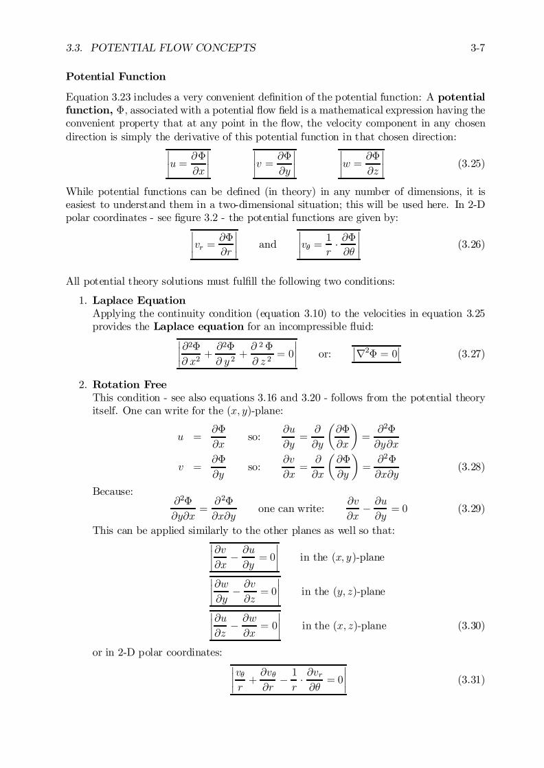
3.3. POTENTIAL FLOW CONCEPTS 3-7
Potential Function
Equation 3.23 includes a very convenient de…nition of the potential function: A potentialfunction, ©; associated with a potential ‡ow …eld is a mathematical expression having theconvenient property that at any point in the ‡ow, the velocity component in any chosendirection is simply the derivative of this potential function in that chosen direction:
¯¯u = @©
@x
¯¯
¯¯v = @©
@y
¯¯
¯¯w = @©
@z
¯¯ (3.25)
While potential functions can be de…ned (in theory) in any number of dimensions, it iseasiest to understand them in a two-dimensional situation; this will be used here. In 2-Dpolar coordinates - see …gure 3.2 - the potential functions are given by:
¯¯vr =
@©
@r
¯¯ and
¯¯vµ =
1
r¢ @©@µ
¯¯ (3.26)
All potential theory solutions must ful…ll the following two conditions:
1. Laplace EquationApplying the continuity condition (equation 3.10) to the velocities in equation 3.25provides the Laplace equation for an incompressible ‡uid:
¯¯@2©@ x2
+@2©
@ y 2+@ 2©
@ z 2= 0
¯¯ or:
¯r2© = 0
¯(3.27)
2. Rotation FreeThis condition - see also equations 3.16 and 3.20 - follows from the potential theoryitself. One can write for the (x; y)-plane:
u =@©
@xso:
@u
@y=@
@y
µ@©
@x
¶=@2©
@y@x
v =@©
@yso:
@v
@x=@
@x
µ@©
@y
¶=@2©
@x@y(3.28)
Because:@2©
@y@x=@2©
@x@yone can write:
@v
@x¡ @u
@y= 0 (3.29)
This can be applied similarly to the other planes as well so that:¯¯@v@x
¡ @u
@y= 0
¯¯ in the (x; y)-plane
¯¯@w@y
¡ @v
@z= 0
¯¯ in the (y; z)-plane
¯¯@u@z
¡ @w
@x= 0
¯¯ in the (x; z)-plane (3.30)
or in 2-D polar coordinates:¯¯vµr+@vµ@r
¡ 1
r¢ @vr@µ
= 0
¯¯ (3.31)
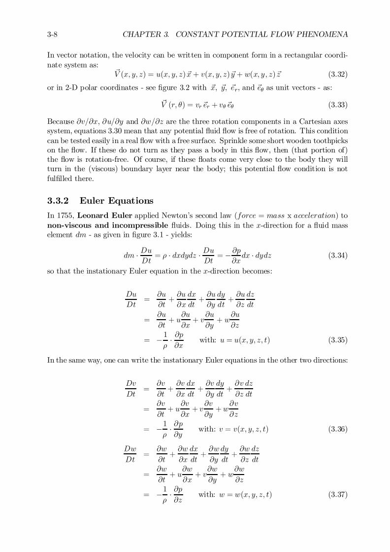
3-8 CHAPTER 3. CONSTANT POTENTIAL FLOW PHENOMENA
In vector notation, the velocity can be written in component form in a rectangular coordi-nate system as:
~V (x; y; z) = u(x; y; z)~x + v(x; y; z)~y + w(x; y; z)~z (3.32)
or in 2-D polar coordinates - see …gure 3.2 with ~x, ~y, ~er, and ~eµ as unit vectors - as:
~V (r; µ) = vr ~er + vµ ~eµ (3.33)
Because @v=@x, @u=@y and @w=@z are the three rotation components in a Cartesian axessystem, equations 3.30 mean that any potential ‡uid ‡ow is free of rotation. This conditioncan be tested easily in a real ‡ow with a free surface. Sprinkle some short wooden toothpickson the ‡ow. If these do not turn as they pass a body in this ‡ow, then (that portion of)the ‡ow is rotation-free. Of course, if these ‡oats come very close to the body they willturn in the (viscous) boundary layer near the body; this potential ‡ow condition is notful…lled there.
3.3.2 Euler Equations
In 1755, Leonard Euler applied Newton’s second law (force = mass x acceleration) tonon-viscous and incompressible ‡uids. Doing this in the x-direction for a ‡uid masselement dm - as given in …gure 3.1 - yields:
dm ¢ DuDt
= ½ ¢ dxdydz ¢ DuDt
= ¡ @p@xdx ¢ dydz (3.34)
so that the instationary Euler equation in the x-direction becomes:
Du
Dt=
@u
@t+@u
@x
dx
dt+@u
@y
dy
dt+@u
@z
dz
dt
=@u
@t+ u
@u
@x+ v
@u
@y+ w
@u
@z
= ¡ 1½
¢ @p@x
with: u = u(x; y; z; t) (3.35)
In the same way, one can write the instationary Euler equations in the other two directions:
Dv
Dt=
@v
@t+@v
@x
dx
dt+@v
@y
dy
dt+@v
@z
dz
dt
=@v
@t+ u
@v
@x+ v
@v
@y+w
@v
@z
= ¡1½
¢ @p@y
with: v = v(x; y; z; t) (3.36)
Dw
Dt=
@w
@t+@w
@x
dx
dt+@w
@y
dy
dt+@w
@z
dz
dt
=@w
@t+ u
@w
@x+ v
@w
@y+ w
@w
@z
= ¡1½
¢ @p@z
with: w = w(x; y; z; t) (3.37)
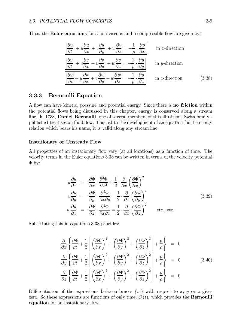
3.3. POTENTIAL FLOW CONCEPTS 3-9
Thus, the Euler equations for a non-viscous and incompressible ‡ow are given by:
¯¯@u@t
+ u@u
@x+ v
@u
@y+w
@u
@z= ¡1
½¢ @p@x
¯¯ in x-direction
¯¯@v@t
+ u@v
@x+ v
@v
@y+ w
@v
@z= ¡1
½¢ @p@y
¯¯ in y-direction
¯¯@w@t+ u
@w
@x+ v
@w
@y+w
@w
@z= ¡1
½¢ @p@z
¯¯ in z-direction (3.38)
3.3.3 Bernoulli Equation
A ‡ow can have kinetic, pressure and potential energy. Since there is no friction withinthe potential ‡ows being discussed in this chapter, energy is conserved along a streamline. In 1738, Daniel Bernoulli, one of several members of this illustrious Swiss family -published treatises on ‡uid ‡ow. This led to the development of an equation for the energyrelation which bears his name; it is valid along any stream line.
Instationary or Unsteady Flow
All properties of an instationary ‡ow vary (at all locations) as a function of time. Thevelocity terms in the Euler equations 3.38 can be written in terms of the velocity potential© by:
u@u
@x=
@©
@x¢ @
2©
@x2=1
2¢ @@x
µ@©
@x
¶2
v@u
@y=
@©
@y¢ @
2©
@x@y=1
2¢ @@x
µ@©
@y
¶2
(3.39)
w@u
@z=
@©
@z¢ @
2©
@x@z=1
2¢ @@x
µ@©
@z
¶2
etc., etc.
Substituting this in equations 3.38 provides:
@
@x
(@©
@t+1
2
"µ@©
@x
¶2
+
µ@©
@y
¶2
+
µ@©
@z
¶2#+p
½
)= 0
@
@y
(@©
@t+1
2
"µ@©
@x
¶2
+
µ@©
@y
¶2
+
µ@©
@z
¶2#+p
½
)= 0 (3.40)
@
@z
(@©
@t+1
2
"µ@©
@x
¶2
+
µ@©
@y
¶2
+
µ@©
@z
¶2#+p
½
)= 0
Di¤erentiation of the expressions between braces f:::g with respect to x, y or z giveszero. So these expressions are functions of only time, C (t), which provides the Bernoulliequation for an instationary ‡ow:
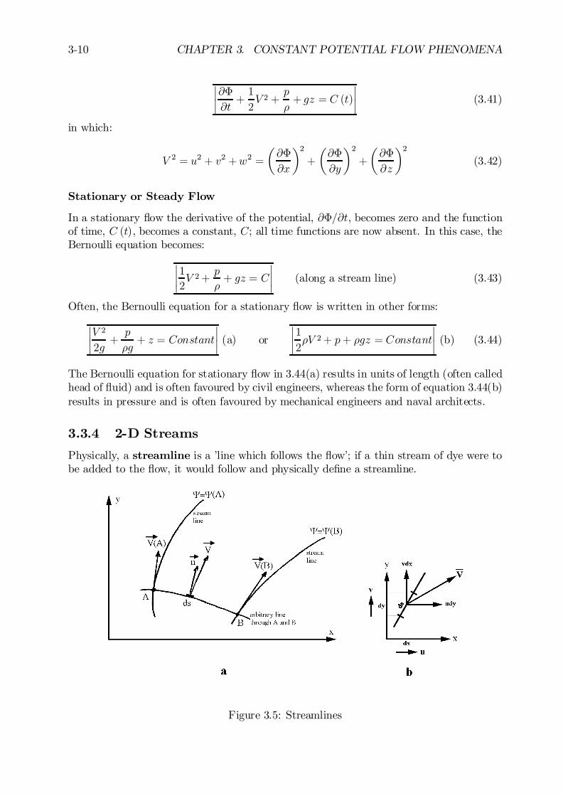
3-10 CHAPTER 3. CONSTANT POTENTIAL FLOW PHENOMENA
¯¯@©@t+1
2V 2 +
p
½+ gz = C (t)
¯¯ (3.41)
in which:
V 2 = u2 + v2 +w2 =
µ@©
@x
¶2+
µ@©
@y
¶2
+
µ@©
@z
¶2(3.42)
Stationary or Steady Flow
In a stationary ‡ow the derivative of the potential, @©=@t, becomes zero and the functionof time, C (t), becomes a constant, C; all time functions are now absent. In this case, theBernoulli equation becomes:
¯¯12V 2+
p
½+ gz = C
¯¯ (along a stream line) (3.43)
Often, the Bernoulli equation for a stationary ‡ow is written in other forms:
¯¯V 22g+p
½g+ z = Constant
¯¯ (a) or
¯¯12½V 2+ p+ ½gz = Constant
¯¯ (b) (3.44)
The Bernoulli equation for stationary ‡ow in 3.44(a) results in units of length (often calledhead of ‡uid) and is often favoured by civil engineers, whereas the form of equation 3.44(b)results in pressure and is often favoured by mechanical engineers and naval architects.
3.3.4 2-D Streams
Physically, a streamline is a ’line which follows the ‡ow’; if a thin stream of dye were tobe added to the ‡ow, it would follow and physically de…ne a streamline.
Figure 3.5: Streamlines
3.3. POTENTIAL FLOW CONCEPTS 3-11
The vector ~n in …gure 3.5 is the normal vector on an arbitrary line through a point A onthe left stream line and a point B on the right stream line.The rate of ‡ow between two streamlines in the (x; y)-plane (see …gures 3.5-a and 3.5-b) isgiven by:
¢ªA!B =
BZ
A
³~V ¢ ~n
´¢ ds =
BZ
A
(u ¢ dy ¡ v ¢ dx)
=
BZ
A
µ@ª
@ydy+
@ª
@xdx
¶=
BZ
A
dª = ª (B)¡ª (A) (3.45)
in which ¢ªA!B is the volume of ‡ow per unit of time between two streamlines throughA and B.
2-D Stream Lines
This rate of ‡ow remains constant when A and B follow their streamlines. The volume of‡ow between any two streamlines is therefore directly proportional to the di¤erence betweenthe - to be de…ned - stream function values of those two stream lines. Furthermore, thevelocity must increase as the streamlines come closer together and decrease as they divergewhile following a stream path. This follows from continuity of the incompressible ‡owMathematically, a streamline is simply a curve for which:
ª = constant (3.46)
Since no ‡ow takes place across streamlines, then in 2-D rectangular coordinates:
dª = u dy ¡ v dx (3.47)
or in 2-D polar coordinates:dª = vr r dµ¡ vµ dr (3.48)
Just like the potential function has a stream function no direct physical meaning; itsderivatives however are very useful.
2-D Stream Function
Much like the potential function de…ned above, the stream function,ª, is a mathematicalexpression such that:
¯¯u = @ª
@y
¯¯ (a) and
¯¯v = ¡@ª
@x
¯¯ (b) (3.49)
or in polar coordinates:
¯¯vr =
1
r¢ @ª@µ
¯¯ (a) and
¯¯vµ = ¡@ª
@r
¯¯ (b) (3.50)
3-12 CHAPTER 3. CONSTANT POTENTIAL FLOW PHENOMENA
3.3.5 Properties
A few basic additional principles are reviewed in this section before continuing with themore classical potential ‡ow mechanics and mathematics.
Orthogonality
The velocity components, u and v , can be expressed in two di¤erent but equivalent ways:¯¯u = @©
@x= +
@ª
@y
¯¯ (a) and
¯¯v = @©
@y= ¡@ª
@x
¯¯ (b) (3.51)
Since @©=@y is the negative reciprocal of @ª=@x, the stream lines and potential lines mustbe orthogonal; the stream lines and potential lines always cross each other at right angles.This fact can be handy when sketching ‡ow patterns using stream lines and potential lines.In 2-D polar coordinates, the velocity components, vr and vµ, are:
¯¯vr = +
@©
@r=1
r¢ @ª@µ
¯¯ (a) and
¯¯vµ =
1
r¢ @©@µ
= ¡@ª@r
¯¯ (b) (3.52)
Impervious Boundary
There is no ‡ow across a streamline so that any impervious ‡ow boundary, therefore,must also be a streamline. This means that:
@©@n= 0
ª = constant
9=; at any impervious boundary (3.53)
in which n is the normal to the (impervious) surface.These are important relations which will be used repeatedly.
Conditions far from a Disturbance
It is usually assumed that nothing special happens as one moves far away from the area ofinterest. In mathematical terms, this means that:
if xÀ 0 and/or y À 0 then: ª! ª1 and © ! ©1 (3.54)
The subscript 1 denotes a condition which exists far away from the location of primaryinterest.
Steady and Unsteady Flow
Steady ‡ow means that at any chosen location - thus also at a point on any givenstreamline - the velocity is constant and independent of time. This means that:
@ ~V
@ t= 0 (steady ‡ow) (3.55)
Obviously, unsteady ‡ow is any ‡ow condition which does not satisfy this relation. Wavesare a good example of unsteady ‡ow, by the way.
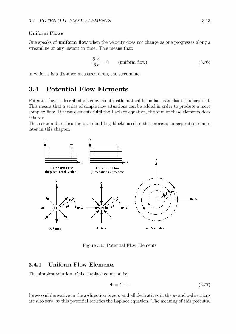
3.4. POTENTIAL FLOW ELEMENTS 3-13
Uniform Flows
One speaks of uniform ‡ow when the velocity does not change as one progresses along astreamline at any instant in time. This means that:
@ ~V
@ s= 0 (uniform ‡ow) (3.56)
in which s is a distance measured along the streamline.
3.4 Potential Flow Elements
Potential ‡ows - described via convenient mathematical formulas - can also be superposed.This means that a series of simple ‡ow situations can be added in order to produce a morecomplex ‡ow. If these elements ful…l the Laplace equation, the sum of these elements doesthis too.This section describes the basic building blocks used in this process; superposition comeslater in this chapter.
Figure 3.6: Potential Flow Elements
3.4.1 Uniform Flow Elements
The simplest solution of the Laplace equation is:
© = U ¢ x (3.57)
Its second derivative in the x-direction is zero and all derivatives in the y- and z-directionsare also zero; so this potential satis…es the Laplace equation. The meaning of this potential
3-14 CHAPTER 3. CONSTANT POTENTIAL FLOW PHENOMENA
is a uniform steady ‡ow in the x-direction, since the only velocity component is u(x; y) = U .This ‡ow has a series of equally spaced parallel stream lines parallel to the x-axis, as shownin …gure 3.6-a. Its stream function follows from:
u =@ª
@y= U so that ª = U ¢ y (3.58)
The ‡ow rate (in m3/s for example - or actually in m2/s because only a unit thickness inthe z-direction is being considered) between any two stream lines separated by an amount¢ª is constant and is proportional to ¢ª (or ¢y as well in this case). Thus for a uniform‡ow in the positive x-direction, the potential and stream functions are given by:
j© = +U ¢ xj (a) and jª = +U ¢ yj (b) (3.59)
If the ‡ow is in the negative x-direction (see …gure 3.6-b), the potential and stream functionswill change sign:
j© = ¡U ¢ xj (a) and jª = ¡U ¢ yj (b) (3.60)
3.4.2 Source and Sink Elements
A source is a point from which ‡ow radiates outward in all directions as shown in …gure3.6-c. Its location is often denoted by a small circle enclosing the letters SO or a plus sign.Its potential and stream functions are given most easily in polar coordinates:
¯¯© = + Q
2¼¢ ln r
¯¯ (a) and
¯¯ª = + Q
2¼¢ µ
¯¯ (b) (3.61)
in which Q is the strength of the source (or ‡ow rate) with units of m2/s for a two-dimensional ‡ow.It requires some algebra to show that this potential satis…es the Laplace equation. Thepotential lines are circles centered at the source location: r = constant; its stream lines areradial lines: µ = constant.The Cartesian expression of the potential and stream functions looks like:
© = +Q
2¼¢ ln
px2 + y2 (a) and ª = +
Q
2¼¢ arctan
³yx
´(b) (3.62)
The velocity in the radial direction can be found from the derivative of the potentialfunction with respect to r, so:
vr =@©
@r=1
r¢ @ª@µ
=Q
2¼r(3.63)
There is no ‡ow in the tangential direction, because:
vµ =1
r¢ @©@µ
= ¡@ª@r
= 0 (3.64)
This ‡ow is called a source ‡ow because the amount of ‡uid passing through a circle atradius r is always Q. The ‡uid is free of rotation, because the source strength, Q, isconstant in the ‡uid. However, the origin, r =
px2 + y2 = 0, is a singular point; the

3.4. POTENTIAL FLOW ELEMENTS 3-15
velocities go to in…nity at this point. Therefore, the potential theory is not valid there andthis point has to be excluded when carrying out integrations in the ‡uid.
A sink is a negative source and thus has an inward radial ‡ow. It is denoted by a circleenclosing the letters SK or a minus sign as shown in …gure 3.6-d. In polar coordinates itcan be expressed as:
¯¯© = ¡ Q
2¼¢ ln r
¯¯ (a) and
¯¯ª = ¡ Q
2¼¢ µ
¯¯ (b) (3.65)
and in Cartesian coordinates as:
© = ¡Q2¼
¢ lnpx2 + y2 (a) and ª = ¡Q
2¼¢ arctan
³yx
´(b) (3.66)
3.4.3 Circulation or Vortex Elements
A circulation or a vortex, ¡, is a tangential ‡ow (circular path) around a point as is shownin …gure 3.6-e. The potential and stream functions are in this case:
¯¯© = + ¡
2¼¢ µ
¯¯ (a) and
¯¯ª = ¡ ¡
2¼¢ ln r
¯¯ (b) (3.67)
or in Cartesian coordinates:
© = +¡
2¼¢ arctan
³ yx
´(a) and ª = ¡ ¡
2¼¢ ln
px2 + y2 (b) (3.68)
The velocities are now in a tangential counter-clockwise direction:
vµ =1
r¢ @©@µ
= ¡@ª@r=
¡
2¼r(3.69)
There is no velocity in radial direction, because:
vr =@©
@r=1
r¢ @ª@µ
= 0 (3.70)
One should remember that the circulation strength, ¡, can be found from:
¡ =
Ivµ ¢ ds = 2¼r ¢ vµ = constant (3.71)
The ‡uid is free of rotation, because the circulation, ¡, is constant in the ‡uid. However,the origin, r =
px2 + y2 = 0, is a singular point; the velocities go to in…nity at this
point. Therefore, potential theory is not valid there and this point has to be excludedwhen carrying out integrations in the ‡uid.
The potential and stream functions of a circulation with tangential velocities in a clockwisedirection are given by:
¯¯© = ¡ ¡
2¼¢ µ
¯¯ (a) and
¯¯ª = + ¡
2¼¢ ln r
¯¯ (b) (3.72)
or in Cartesian coordinates by:
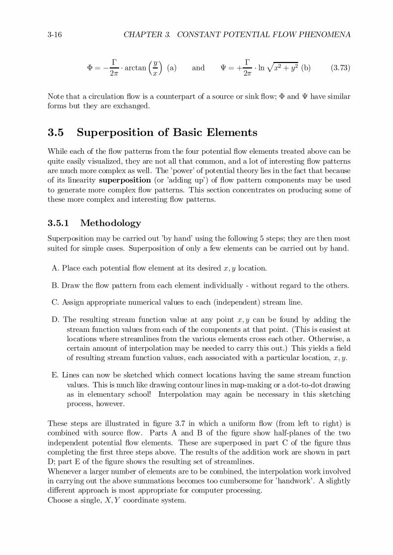
3-16 CHAPTER 3. CONSTANT POTENTIAL FLOW PHENOMENA
© = ¡ ¡
2¼¢ arctan
³ yx
´(a) and ª = +
¡
2¼¢ ln
px2 + y2 (b) (3.73)
Note that a circulation ‡ow is a counterpart of a source or sink ‡ow; © and ª have similarforms but they are exchanged.
3.5 Superposition of Basic Elements
While each of the ‡ow patterns from the four potential ‡ow elements treated above can bequite easily visualized, they are not all that common, and a lot of interesting ‡ow patternsare much more complex as well. The ’power’ of potential theory lies in the fact that becauseof its linearity superposition (or ’adding up’) of ‡ow pattern components may be usedto generate more complex ‡ow patterns. This section concentrates on producing some ofthese more complex and interesting ‡ow patterns.
3.5.1 Methodology
Superposition may be carried out ’by hand’ using the following 5 steps; they are then mostsuited for simple cases. Superposition of only a few elements can be carried out by hand.
A. Place each potential ‡ow element at its desired x; y location.
B. Draw the ‡ow pattern from each element individually - without regard to the others.
C. Assign appropriate numerical values to each (independent) stream line.
D. The resulting stream function value at any point x; y can be found by adding thestream function values from each of the components at that point. (This is easiest atlocations where streamlines from the various elements cross each other. Otherwise, acertain amount of interpolation may be needed to carry this out.) This yields a …eldof resulting stream function values, each associated with a particular location, x; y:
E. Lines can now be sketched which connect locations having the same stream functionvalues. This is much like drawing contour lines in map-making or a dot-to-dot drawingas in elementary school! Interpolation may again be necessary in this sketchingprocess, however.
These steps are illustrated in …gure 3.7 in which a uniform ‡ow (from left to right) iscombined with source ‡ow. Parts A and B of the …gure show half-planes of the twoindependent potential ‡ow elements. These are superposed in part C of the …gure thuscompleting the …rst three steps above. The results of the addition work are shown in partD; part E of the …gure shows the resulting set of streamlines.Whenever a larger number of elements are to be combined, the interpolation work involvedin carrying out the above summations becomes too cumbersome for ’handwork’. A slightlydi¤erent approach is most appropriate for computer processing.Choose a single, X;Y coordinate system.
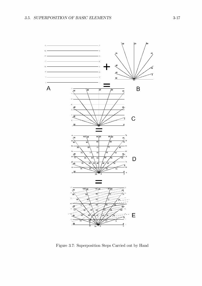
3.5. SUPERPOSITION OF BASIC ELEMENTS 3-17
Figure 3.7: Superposition Steps Carried out by Hand
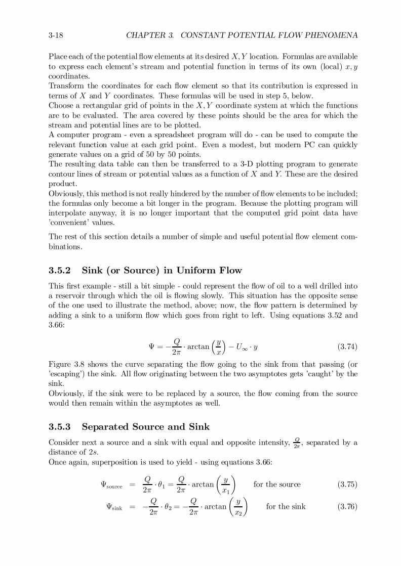
3-18 CHAPTER 3. CONSTANT POTENTIAL FLOW PHENOMENA
Place each of the potential ‡owelements at its desired X;Y location. Formulas are availableto express each element’s stream and potential function in terms of its own (local) x; ycoordinates.Transform the coordinates for each ‡ow element so that its contribution is expressed interms of X and Y coordinates. These formulas will be used in step 5, below.Choose a rectangular grid of points in the X;Y coordinate system at which the functionsare to be evaluated. The area covered by these points should be the area for which thestream and potential lines are to be plotted.A computer program - even a spreadsheet program will do - can be used to compute therelevant function value at each grid point. Even a modest, but modern PC can quicklygenerate values on a grid of 50 by 50 points.The resulting data table can then be transferred to a 3-D plotting program to generatecontour lines of stream or potential values as a function of X and Y: These are the desiredproduct.Obviously, this method is not really hindered by the number of ‡ow elements to be included;the formulas only become a bit longer in the program. Because the plotting program willinterpolate anyway, it is no longer important that the computed grid point data have’convenient’ values.
The rest of this section details a number of simple and useful potential ‡ow element com-binations.
3.5.2 Sink (or Source) in Uniform Flow
This …rst example - still a bit simple - could represent the ‡ow of oil to a well drilled intoa reservoir through which the oil is ‡owing slowly. This situation has the opposite senseof the one used to illustrate the method, above; now, the ‡ow pattern is determined byadding a sink to a uniform ‡ow which goes from right to left. Using equations 3.52 and3.66:
ª = ¡ Q
2¼¢ arctan
³ yx
´¡ U1 ¢ y (3.74)
Figure 3.8 shows the curve separating the ‡ow going to the sink from that passing (or’escaping’) the sink. All ‡ow originating between the two asymptotes gets ’caught’ by thesink.Obviously, if the sink were to be replaced by a source, the ‡ow coming from the sourcewould then remain within the asymptotes as well.
3.5.3 Separated Source and Sink
Consider next a source and a sink with equal and opposite intensity, Q2¼
, separated by adistance of 2s:Once again, superposition is used to yield - using equations 3.66:
ªsource =Q
2¼¢ µ1 =
Q
2¼¢ arctan
µy
x1
¶for the source (3.75)
ªsink = ¡Q2¼
¢ µ2 = ¡Q2¼
¢ arctanµy
x2
¶for the sink (3.76)
3.5. SUPERPOSITION OF BASIC ELEMENTS 3-19
Figure 3.8: Sink in a Uniform Flow
The resulting stream lines are then (in polar coordinates for a change) lines with:
ª =Q
2¼¢ µ1 ¡ Q
2¼¢ µ2 = constant (3.77)
These stream lines are a set of circles, all centered on the y axis, and all passing throughsource and sink; see …gure 3.9.
Figure 3.9: Separated Source and Sink
One can also write the resultant stream function in Cartesian coordinates as:
ª =Q
2¼¢ arctan
µ2 y s
x2+ y2 ¡ s2¶
(3.78)
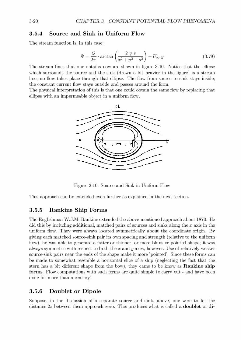
3-20 CHAPTER 3. CONSTANT POTENTIAL FLOW PHENOMENA
3.5.4 Source and Sink in Uniform Flow
The stream function is, in this case:
ª =Q
2¼¢ arctan
µ2 y s
x2 + y2 ¡ s2¶+ U1 y (3.79)
The stream lines that one obtains now are shown in …gure 3.10. Notice that the ellipsewhich surrounds the source and the sink (drawn a bit heavier in the …gure) is a streamline; no ‡ow takes place through that ellipse. The ‡ow from source to sink stays inside;the constant current ‡ow stays outside and passes around the form.The physical interpretation of this is that one could obtain the same ‡ow by replacing thatellipse with an impermeable object in a uniform ‡ow.
Figure 3.10: Source and Sink in Uniform Flow
This approach can be extended even further as explained in the next section.
3.5.5 Rankine Ship Forms
The Englishman W.J.M. Rankine extended the above-mentioned approach about 1870. Hedid this by including additional, matched pairs of sources and sinks along the x axis in theuniform ‡ow. They were always located symmetrically about the coordinate origin. Bygiving each matched source-sink pair its own spacing and strength (relative to the uniform‡ow), he was able to generate a fatter or thinner, or more blunt or pointed shape; it wasalways symmetric with respect to both the x and y axes, however. Use of relatively weakersource-sink pairs near the ends of the shape make it more ’pointed’. Since these forms canbe made to somewhat resemble a horizontal slice of a ship (neglecting the fact that thestern has a bit di¤erent shape from the bow), they came to be know as Rankine shipforms. Flow computations with such forms are quite simple to carry out - and have beendone for more than a century!
3.5.6 Doublet or Dipole
Suppose, in the discussion of a separate source and sink, above, one were to let thedistance 2s between them approach zero. This produces what is called a doublet or di-

3.5. SUPERPOSITION OF BASIC ELEMENTS 3-21
pole. The corresponding stream function is found by letting s approach zero in equation3.78:
ª = lims!0
½Q
2¼¢ arctan
µ2y s
x2 + y2 ¡ s2¶¾
(3.80)
As x! 0 then arctan(x)! x, so that:
ª = lims!0
½Q
¼s ¢
µy
x2 + y2¡ s2¶¾
(3.81)
One must keep the term Q¼s (that is renamed the doublet strength, ¹) constant and non-
zero (otherwise there won’t be anything left; the origin is a singular point anyway!). Onthe other hand, s2 becomes small even faster so that it can be neglected relative to x2+y2.After a bit of algebra, the above stream function becomes:
¯¯ª = ¹ ¢ y
x2 + y2=¹ ¢ sin µr
¯¯ (3.82)
and similarly:¯¯© = ¹ ¢ x
x2 + y2=¹ ¢ cos µr
¯¯ (3.83)
In …gure 3.11, both the stream (solid) and equipotential (dashed) lines are circles centeredon the y and x axes respectively. All the circles pass through the origin, too.
Figure 3.11: Doublet or Dipole Flow
3.5.7 Doublet in Uniform Flow
The next step is to add a uniform ‡ow to the doublet just discussed. If the ‡ow goes alongthe negative x-axis, this yields:
ª =¹ ¢ yx2 + y2
¡ U1 y (3.84)
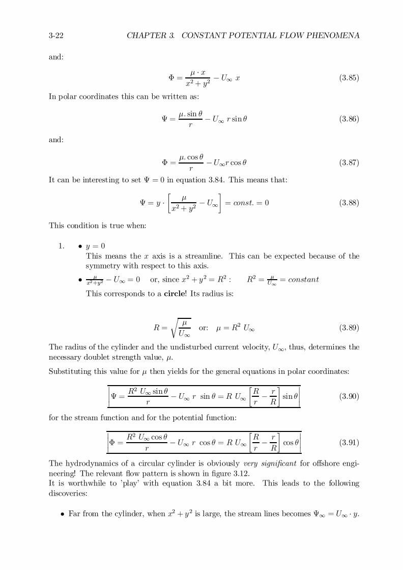
3-22 CHAPTER 3. CONSTANT POTENTIAL FLOW PHENOMENA
and:
© =¹ ¢ xx2+ y2
¡ U1 x (3.85)
In polar coordinates this can be written as:
ª =¹: sin µ
r¡ U1 r sin µ (3.86)
and:
© =¹: cos µ
r¡U1r cos µ (3.87)
It can be interesting to set ª = 0 in equation 3.84. This means that:
ª = y ¢·
¹
x2+ y2¡ U1
¸= const: = 0 (3.88)
This condition is true when:
1. ² y = 0This means the x axis is a streamline. This can be expected because of thesymmetry with respect to this axis.
² ¹x2+y2 ¡ U1 = 0 or, since x2 + y2 = R2 : R2 = ¹
U1= constant
This corresponds to a circle! Its radius is:
R =
r¹
U1or: ¹ = R2 U1 (3.89)
The radius of the cylinder and the undisturbed current velocity, U1; thus, determines thenecessary doublet strength value, ¹.
Substituting this value for ¹ then yields for the general equations in polar coordinates:
¯¯ª = R
2 U1 sin µr
¡ U1 r sin µ = R U1·R
r¡ r
R
¸sin µ
¯¯ (3.90)
for the stream function and for the potential function:
¯¯© = R
2 U1 cos µr
¡ U1 r cos µ = R U1·R
r¡ r
R
¸cos µ
¯¯ (3.91)
The hydrodynamics of a circular cylinder is obviously very signi…cant for o¤shore engi-neering! The relevant ‡ow pattern is shown in …gure 3.12.It is worthwhile to ’play’ with equation 3.84 a bit more. This leads to the followingdiscoveries:
² Far from the cylinder, when x2 + y2 is large, the stream lines becomes ª1 = U1 ¢ y.
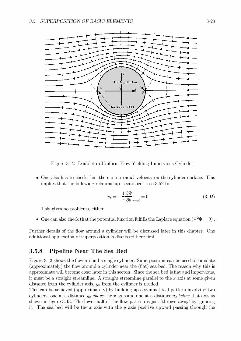
3.5. SUPERPOSITION OF BASIC ELEMENTS 3-23
Figure 3.12: Doublet in Uniform Flow Yielding Impervious Cylinder
² One also has to check that there is no radial velocity on the cylinder surface. Thisimplies that the following relationship is satis…ed - see 3.52-b:
vr = ¡1r
@ª
@µ r=R= 0 (3.92)
This gives no problems, either.
² One can also check that the potential function ful…lls the Laplace equation (O2© = 0) :
Further details of the ‡ow around a cylinder will be discussed later in this chapter. Oneadditional application of superposition is discussed here …rst.
3.5.8 Pipeline Near The Sea Bed
Figure 3.12 shows the ‡ow around a single cylinder. Superposition can be used to simulate(approximately) the ‡ow around a cylinder near the (‡at) sea bed. The reason why this isapproximate will become clear later in this secton. Since the sea bed is ‡at and impervious,it must be a straight streamline. A straight streamline parallel to the x axis at some givendistance from the cylinder axis, y0 from the cylinder is needed.This can be achieved (approximately) by building up a symmetrical pattern involving twocylinders, one at a distance y0 above the x axis and one at a distance y0 below that axis asshown in …gure 3.13. The lower half of the ‡ow pattern is just ’thrown away’ by ignoringit. The sea bed will be the x axis with the y axis positive upward passing through the
3-24 CHAPTER 3. CONSTANT POTENTIAL FLOW PHENOMENA
cylinder center. This special form of superposition is often referred to as re‡ection (aboutthe sea bed, in this case). Re‡ection is commonly used for other applications with the seasurface or even a vertical plane of symmetry as the re‡ection plane.
Figure 3.13: Use of Re‡ection to Get Pipeline Near Sea Bed
This is solved by superposing the solutions for a doublet in a uniform ‡ow above the bedwith one below the bed. All of this yields (after transforming coordinates):
ª = ¹ ¢ y ¡ y0x2+ (y ¡ y0)2
+ ¹ ¢ y + y0
x2 + (y + y0)2 ¡ U1 y (3.93)
By letting y equal zero (at the sea bed) in this equation, one can check that ª remainsconstant and equal to zero in order to prove that the sea bed is indeed a streamline; thisis left to the reader.A more interesting (and more complicated) check is to see if the surface of the pipelineR2 = x2 + (y ¡ y0)2 is still a streamline and thus is (still) impermeable. A quick wayto disprove this can be to check the value of ª at a few convenient points on the circlerepresenting the pipeline. If the values of ª computed at these points on the circle arenot identical, then the circle can no longer be a stream line. It can be convenient to selectlocations such as the top, bottom, front and back of the pipe for this check as is done inthe table below.
Location x y ª
Top 0 y0 + R ¹ ¢³1R+ 1
2y0+R
´¡ U1 ¢ (y0 + R)
Front +R y0 ¹ ¢³
2y0R2+4y20
´¡ U1 ¢ y0
Bottom 0 y0 ¡R ¹ ¢³¡ 1R +
12y0¡R
´¡ U1 ¢ (y0 ¡R)
Back ¡R y0 ¹ ¢³
2y0R2+4y20
´¡ U1 ¢ y0
One can quickly see from this table that the pipeline’s circular surface is no longer astreamline. Why should this be so? The answer lies in the fact that the in‡uence fromeach potential ‡ow element extends (theoretically) to in…nity. Since it has been shownabove that a single doublet pair in a uniform ‡ow does yield a perfect circular section,then it is only to be expected that this circular streamline will be disturbed a bit by thein‡uence of the second doublet introduced in order to make a symmetric pattern withrespect to the sea bed. This is why the word ’approximate’ was used so rigorously at thebeginning of this discussion.
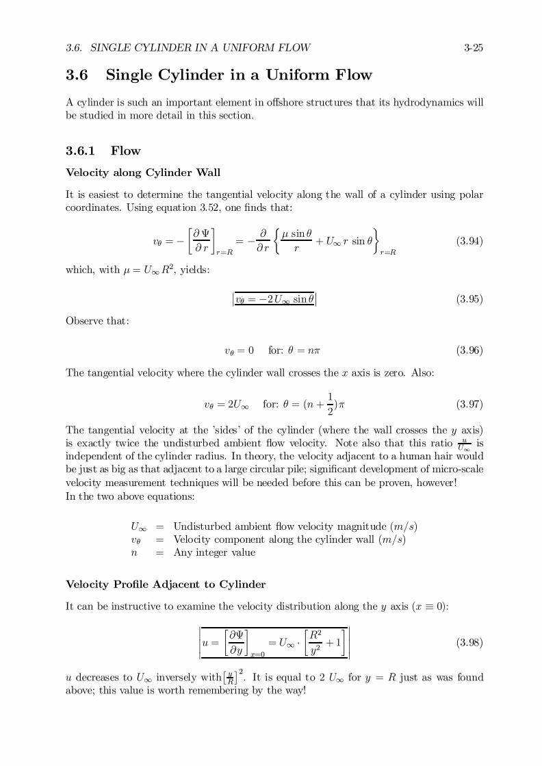
3.6. SINGLE CYLINDER IN A UNIFORM FLOW 3-25
3.6 Single Cylinder in a Uniform Flow
A cylinder is such an important element in o¤shore structures that its hydrodynamics willbe studied in more detail in this section.
3.6.1 Flow
Velocity along Cylinder Wall
It is easiest to determine the tangential velocity along the wall of a cylinder using polarcoordinates. Using equation 3.52, one …nds that:
vµ = ¡·@ ª
@ r
¸
r=R
= ¡ @
@ r
½¹ sin µ
r+ U1 r sin µ
¾
r=R
(3.94)
which, with ¹= U1R2, yields:
¯vµ = ¡2U1 sin µ
¯(3.95)
Observe that:
vµ = 0 for: µ = n¼ (3.96)
The tangential velocity where the cylinder wall crosses the x axis is zero. Also:
vµ = 2U1 for: µ = (n +1
2)¼ (3.97)
The tangential velocity at the ’sides’ of the cylinder (where the wall crosses the y axis)is exactly twice the undisturbed ambient ‡ow velocity. Note also that this ratio u
U1is
independent of the cylinder radius. In theory, the velocity adjacent to a human hair wouldbe just as big as that adjacent to a large circular pile; signi…cant development of micro-scalevelocity measurement techniques will be needed before this can be proven, however!In the two above equations:
U1 = Undisturbed ambient ‡ow velocity magnitude (m=s)vµ = Velocity component along the cylinder wall (m=s)n = Any integer value
Velocity Pro…le Adjacent to Cylinder
It can be instructive to examine the velocity distribution along the y axis (x ´ 0):
¯¯¯u =
·@ª
@y
¸
x=0
= U1 ¢·R2
y2+1
¸¯¯¯ (3.98)
u decreases to U1 inversely with£yR
¤2. It is equal to 2 U1 for y = R just as was found
above; this value is worth remembering by the way!
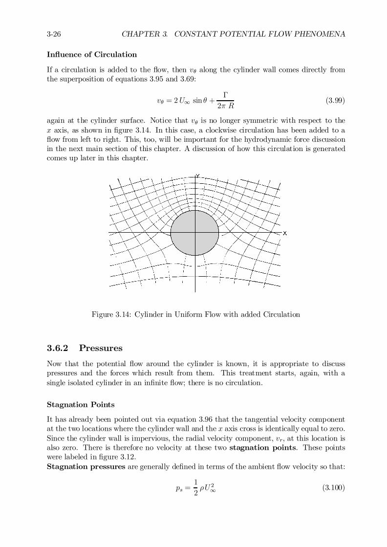
3-26 CHAPTER 3. CONSTANT POTENTIAL FLOW PHENOMENA
In‡uence of Circulation
If a circulation is added to the ‡ow, then vµ along the cylinder wall comes directly fromthe superposition of equations 3.95 and 3.69:
vµ = 2U1 sin µ +¡
2¼ R(3.99)
again at the cylinder surface. Notice that vµ is no longer symmetric with respect to thex axis, as shown in …gure 3.14. In this case, a clockwise circulation has been added to a‡ow from left to right. This, too, will be important for the hydrodynamic force discussionin the next main section of this chapter. A discussion of how this circulation is generatedcomes up later in this chapter.
Figure 3.14: Cylinder in Uniform Flow with added Circulation
3.6.2 Pressures
Now that the potential ‡ow around the cylinder is known, it is appropriate to discusspressures and the forces which result from them. This treatment starts, again, with asingle isolated cylinder in an in…nite ‡ow; there is no circulation.
Stagnation Points
It has already been pointed out via equation 3.96 that the tangential velocity componentat the two locations where the cylinder wall and the x axis cross is identically equal to zero.Since the cylinder wall is impervious, the radial velocity component, vr, at this location isalso zero. There is therefore no velocity at these two stagnation points. These pointswere labeled in …gure 3.12.Stagnation pressures are generally de…ned in terms of the ambient ‡ow velocity so that:
ps =1
2½U 21 (3.100)
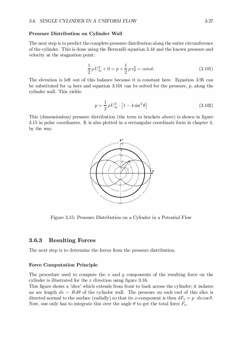
3.6. SINGLE CYLINDER IN A UNIFORM FLOW 3-27
Pressure Distribution on Cylinder Wall
The next step is to predict the complete pressure distribution along the entire circumferenceof the cylinder. This is done using the Bernoulli equation 3.44 and the known pressure andvelocity at the stagnation point:
1
2½ U21+ 0 = p+
1
2½ v2µ = const: (3.101)
The elevation is left out of this balance because it is constant here. Equation 3.95 canbe substituted for vµ here and equation 3.101 can be solved for the pressure, p, along thecylinder wall. This yields:
p =1
2½U 21 ¢
£1¡ 4 sin2 µ
¤(3.102)
This (dimensionless) pressure distribution (the term in brackets above) is shown in …gure3.15 in polar coordinates. It is also plotted in a rectangular coordinate form in chapter 4,by the way.
Figure 3.15: Pressure Distribution on a Cylinder in a Potential Flow
3.6.3 Resulting Forces
The next step is to determine the forces from the pressure distribution.
Force Computation Principle
The procedure used to compute the x and y components of the resulting force on thecylinder is illustrated for the x direction using …gure 3.16.This …gure shows a ’slice’ which extends from front to back across the cylinder; it isolatesan arc length ds = Rdµ of the cylinder wall. The pressure on each end of this slice isdirected normal to the surface (radially) so that its x-component is then dFx = p ¢ ds cos µ.Now, one only has to integrate this over the angle µ to get the total force Fx.
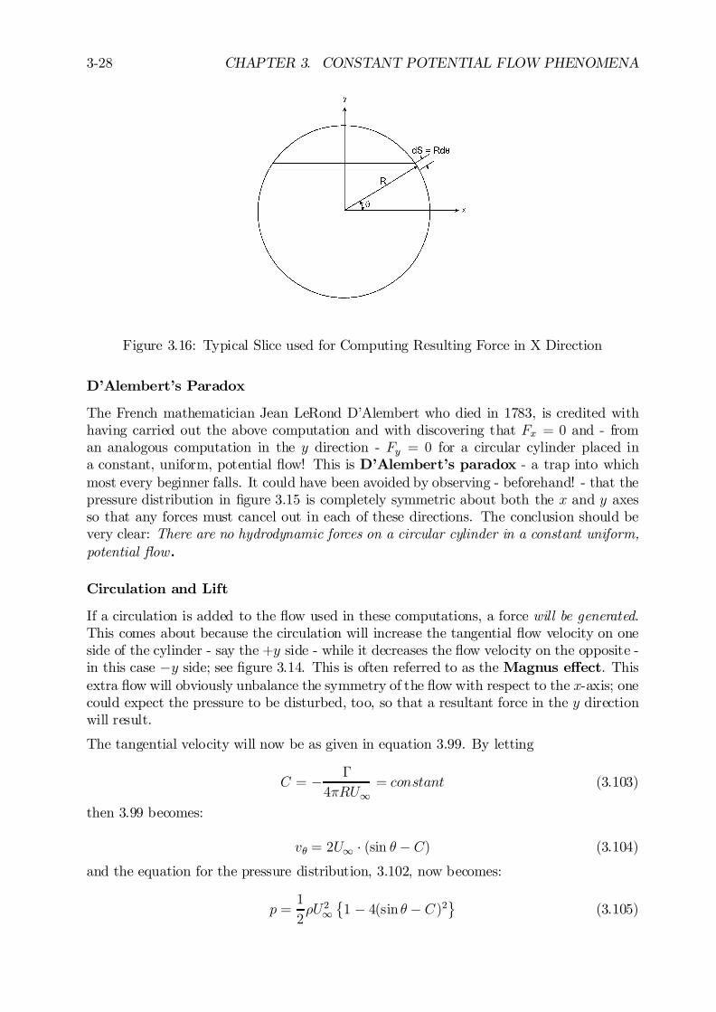
3-28 CHAPTER 3. CONSTANT POTENTIAL FLOW PHENOMENA
Figure 3.16: Typical Slice used for Computing Resulting Force in X Direction
D’Alembert’s Paradox
The French mathematician Jean LeRond D’Alembert who died in 1783, is credited withhaving carried out the above computation and with discovering that Fx = 0 and - froman analogous computation in the y direction - Fy = 0 for a circular cylinder placed ina constant, uniform, potential ‡ow! This is D’Alembert’s paradox - a trap into whichmost every beginner falls. It could have been avoided by observing - beforehand! - that thepressure distribution in …gure 3.15 is completely symmetric about both the x and y axesso that any forces must cancel out in each of these directions. The conclusion should bevery clear: There are no hydrodynamic forces on a circular cylinder in a constant uniform,potential ‡ow.
Circulation and Lift
If a circulation is added to the ‡ow used in these computations, a force will be generated.This comes about because the circulation will increase the tangential ‡ow velocity on oneside of the cylinder - say the +y side - while it decreases the ‡ow velocity on the opposite -in this case ¡y side; see …gure 3.14. This is often referred to as the Magnus e¤ect. Thisextra ‡ow will obviously unbalance the symmetry of the ‡ow with respect to the x-axis; onecould expect the pressure to be disturbed, too, so that a resultant force in the y directionwill result.
The tangential velocity will now be as given in equation 3.99. By letting
C = ¡ ¡
4¼RU1= constant (3.103)
then 3.99 becomes:
vµ = 2U1 ¢ (sin µ¡ C) (3.104)
and the equation for the pressure distribution, 3.102, now becomes:
p =1
2½U21
©1 ¡ 4(sin µ¡ C)2
ª(3.105)
3.6. SINGLE CYLINDER IN A UNIFORM FLOW 3-29
The drag force can be evaluated just as was done above; this still yields a zero resultant,independent of the value of C:The resulting force crosswise to the ‡ow can be found by integrating the y-component ofthe pressure force as follows:
Fy = R
Z 2¼
0
p sin µ dµ (3.106)
After a bit of substitution and algebra one should …nd that:
Fy = 4¼ R ½ U21 C (3.107)
This resultant force is called lift; it is directed perpendicular to the direction of the undis-turbed approaching ‡ow. Notice that the lift force is only present when C 6= 0:Lift forces are responsible for keeping aircraft airborne. The necessary tangential velocitydi¤erential is achieved by making the ‡ow path over the top of a wing or helicopter rotorlonger than the ‡ow path on the underside so that the ‡ow over the top must travel fasterto pass the object in the same time interval. This same phenomenon is important withship’s propellers, too; see chapter 4.Lift is largely responsible for driving a sailboat forward when it is sailing ’close-hauled’.The necessary low pressure ’behind’ the main sail is now created by the jet caused by thejib or foresail. In tennis or with a baseball pitch, a spinning ball will curve one way oranother. Now the ambient air remains stationary while the ball speeds through it. Thenecessary circulation is created by friction between the spinning ball and the air. Sincefriction is involved in this case, discussion will have to be delayed until the next chapter.

3-30 CHAPTER 3. CONSTANT POTENTIAL FLOW PHENOMENA
.
Chapter 4
CONSTANT REAL FLOWPHENOMENA
4.1 Introduction
Now that the basics of constant idealized potential ‡ows have been discussed in the previouschapter, the next step is to consider more realistic - but still constant - ‡ows. The factsthat there is no drag force in a potential ‡ow and that a circulation is required to generatea lift force is true only for a potential (non-viscous) ‡ow. The results from this chapterwith real ‡ows which include viscous e¤ects will be more realistic.The initial discussion of some basic concepts motivates attention for two common dimen-sionless numbers, Rn and Fn, which are handled more generally in Appendix B. These areused to characterize constant ‡ows abound cylinders and ships - and the resultant forces- discussed in the latter part of the chapter. Propulsion systems are handled toward theend of the chapter.
4.2 Basic Viscous Flow Concepts
This section discusses a few basic principles of constant viscous ‡ows. These supplementthe discussion on potential ‡ows given in the …rst parts of chapter 3.
4.2.1 Boundary Layer and Viscosity
In 1883, Osborne Reynolds, an English investigator, observed the ‡ow of water through aglass pipe which drained a container water as shown somewhat schematically in …gure 4.1.He …rst …lled the tank with the drain closed so that the water could come to rest.After opening the drain valve, he found that the ‡ow and streamlines - visualized by astream of ink:
² The streamlines were straight and parallel in the …rst segment of the pipe just down-stream from its entrance.
² The ‡ow velocity near the pipe wall was less than that near the axis of the pipe.0J.M.J. Journée and W.W. Massie, ”OFFSHORE HYDROMECHANICS”, First Edition, January 2001,
Delft University of Technology. For updates see web site: http://www.shipmotions.nl.
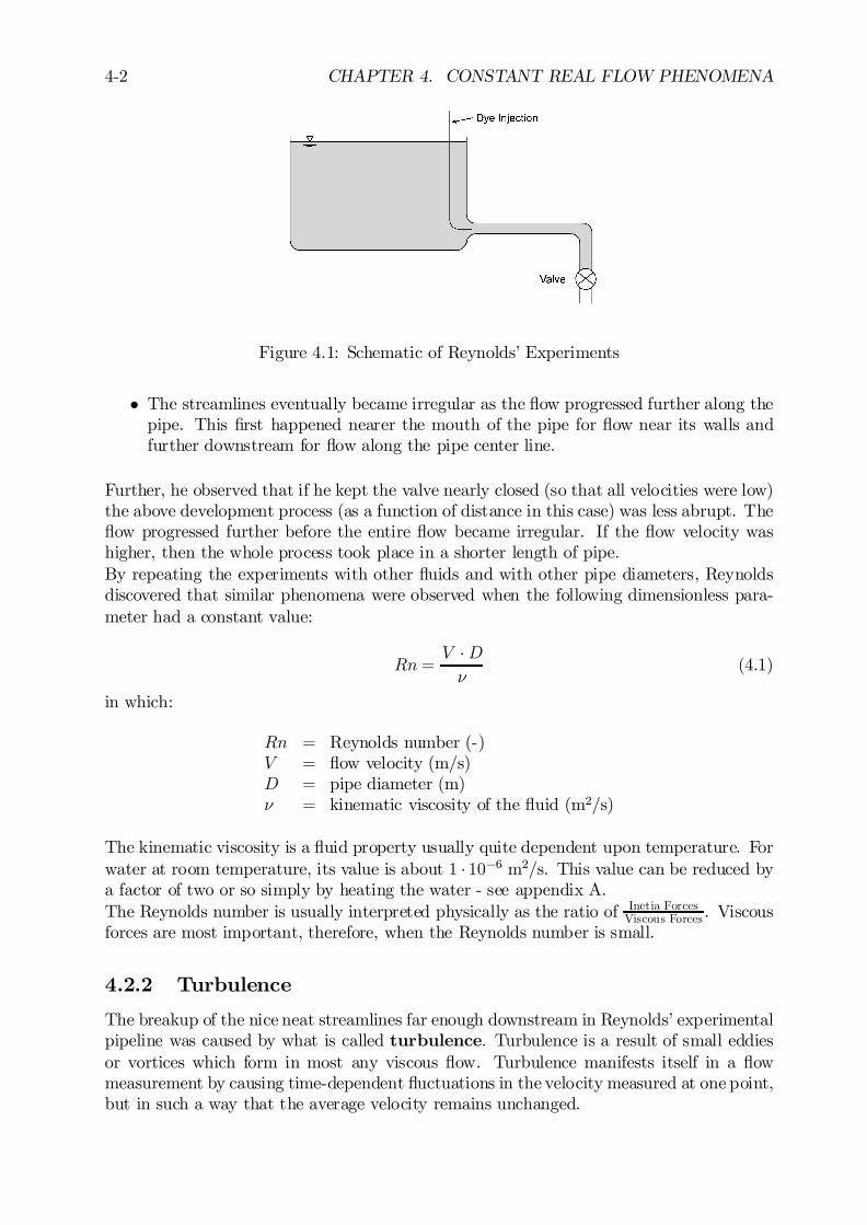
4-2 CHAPTER 4. CONSTANT REAL FLOW PHENOMENA
Figure 4.1: Schematic of Reynolds’ Experiments
² The streamlines eventually became irregular as the ‡ow progressed further along thepipe. This …rst happened nearer the mouth of the pipe for ‡ow near its walls andfurther downstream for ‡ow along the pipe center line.
Further, he observed that if he kept the valve nearly closed (so that all velocities were low)the above development process (as a function of distance in this case) was less abrupt. The‡ow progressed further before the entire ‡ow became irregular. If the ‡ow velocity washigher, then the whole process took place in a shorter length of pipe.By repeating the experiments with other ‡uids and with other pipe diameters, Reynoldsdiscovered that similar phenomena were observed when the following dimensionless para-meter had a constant value:
Rn =V ¢Dº
(4.1)
in which:
Rn = Reynolds number (-)V = ‡ow velocity (m/s)D = pipe diameter (m)º = kinematic viscosity of the ‡uid (m2/s)
The kinematic viscosity is a ‡uid property usually quite dependent upon temperature. Forwater at room temperature, its value is about 1 ¢ 10¡6 m2/s. This value can be reduced bya factor of two or so simply by heating the water - see appendix A.The Reynolds number is usually interpreted physically as the ratio of Inetia Forces
Viscous Forces . Viscousforces are most important, therefore, when the Reynolds number is small.
4.2.2 Turbulence
The breakup of the nice neat streamlines far enough downstream in Reynolds’ experimentalpipeline was caused by what is called turbulence. Turbulence is a result of small eddiesor vortices which form in most any viscous ‡ow. Turbulence manifests itself in a ‡owmeasurement by causing time-dependent ‡uctuations in the velocity measured at one point,but in such a way that the average velocity remains unchanged.
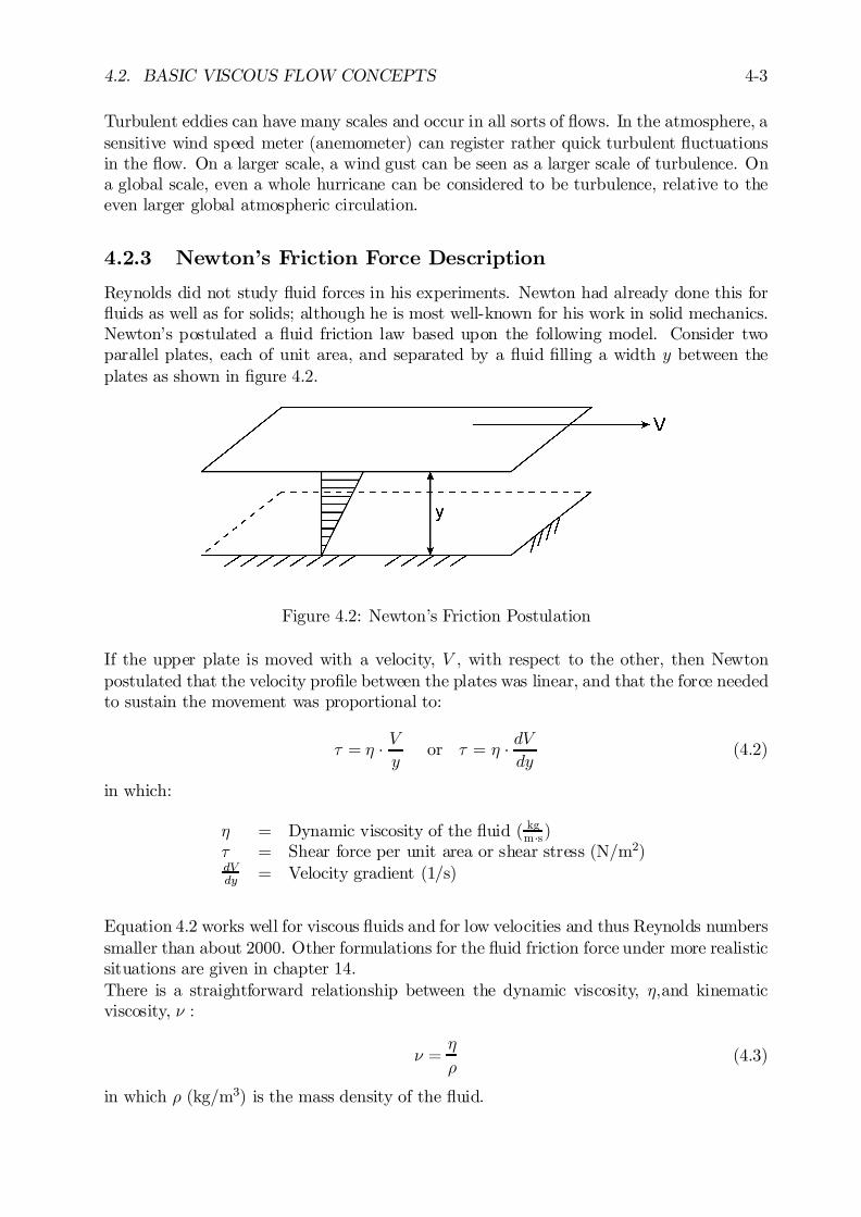
4.2. BASIC VISCOUS FLOW CONCEPTS 4-3
Turbulent eddies can have many scales and occur in all sorts of ‡ows. In the atmosphere, asensitive wind speed meter (anemometer) can register rather quick turbulent ‡uctuationsin the ‡ow. On a larger scale, a wind gust can be seen as a larger scale of turbulence. Ona global scale, even a whole hurricane can be considered to be turbulence, relative to theeven larger global atmospheric circulation.
4.2.3 Newton’s Friction Force Description
Reynolds did not study ‡uid forces in his experiments. Newton had already done this for‡uids as well as for solids; although he is most well-known for his work in solid mechanics.Newton’s postulated a ‡uid friction law based upon the following model. Consider twoparallel plates, each of unit area, and separated by a ‡uid …lling a width y between theplates as shown in …gure 4.2.
Figure 4.2: Newton’s Friction Postulation
If the upper plate is moved with a velocity, V , with respect to the other, then Newtonpostulated that the velocity pro…le between the plates was linear, and that the force neededto sustain the movement was proportional to:
¿ = ´ ¢ Vy
or ¿ = ´ ¢ dVdy
(4.2)
in which:
´ = Dynamic viscosity of the ‡uid ( kgm¢s)
¿ = Shear force per unit area or shear stress (N/m2)dVdy = Velocity gradient (1/s)
Equation 4.2 works well for viscous ‡uids and for low velocities and thus Reynolds numberssmaller than about 2000. Other formulations for the ‡uid friction force under more realisticsituations are given in chapter 14.There is a straightforward relationship between the dynamic viscosity, ´;and kinematicviscosity, º :
º =´
½(4.3)
in which ½ (kg/m3) is the mass density of the ‡uid.
4-4 CHAPTER 4. CONSTANT REAL FLOW PHENOMENA
4.3 Dimensionless Ratios and Scaling Laws
One dimensionless ratio - the Reynolds number - has already been introduced above. Thissection discusses this and one additional common dimensionless number: the Froude num-ber. These are both commonly found in o¤shore hydromechanics.Dimensionless ratios are used to characterize families of di¤erent conditions in an e¢cientway. Reynolds used a single number above to characterize ‡ows of di¤erent ‡uids throughdi¤erent diameter pipes and at di¤erent velocities. His Reynolds number convenientlycombined the three independent variables to form a single one. As long as a consistent setof units is used - it makes no di¤erence if the velocity has been measured in meters persecond, feet per minute, or even leagues per fortnight!For example, by using the Reynolds number to characterize the ‡ow in a pipeline, it ispossible to calibrate a venturi or ori…ce meter using a ‡ow of water even though the metermay later be used to measure a ‡ow of something more exotic like supercritical steam oreven molten sodium.A second use of dimensionless numbers is to correlate (or convert) measurements madeon small physical models to equivalent values for a full-sized or prototype situation. Thisallows experiments to be carried out on a series of relatively inexpensive physical modelsrather than having to build as many full-sized ships (or other objects) instead.
Dimensionless numbers will be used for both purposes later in this chapter. The remainderof this section is concerned primarily with physical models, however.
4.3.1 Physical Model Relationships
Physical model experiments require some form of similarity between the prototype and themodel:
- Geometric similarity: The model must have physical dimensions which are uni-formly proportional to those of the prototype; it must have the same shape.
- Kinematic similarity: Velocities in the model must be proportional to those in theprototype.
- Dynamic similarity: Forces and accelerations in the model must be proportionalto those in the prototype.
These three similarities require that all location vectors, velocity vectors and force vectorsin the coincident coordinates of the scaled model and the prototype have the same direction(argument) and that the magnitude of these vectors (modulus) must relate to each otherin a constant proportion.
If ® - a number larger than 1 - is used to denote the ratio between the prototype (subscriptp) quantity and the model (subscript m) quantity, then:
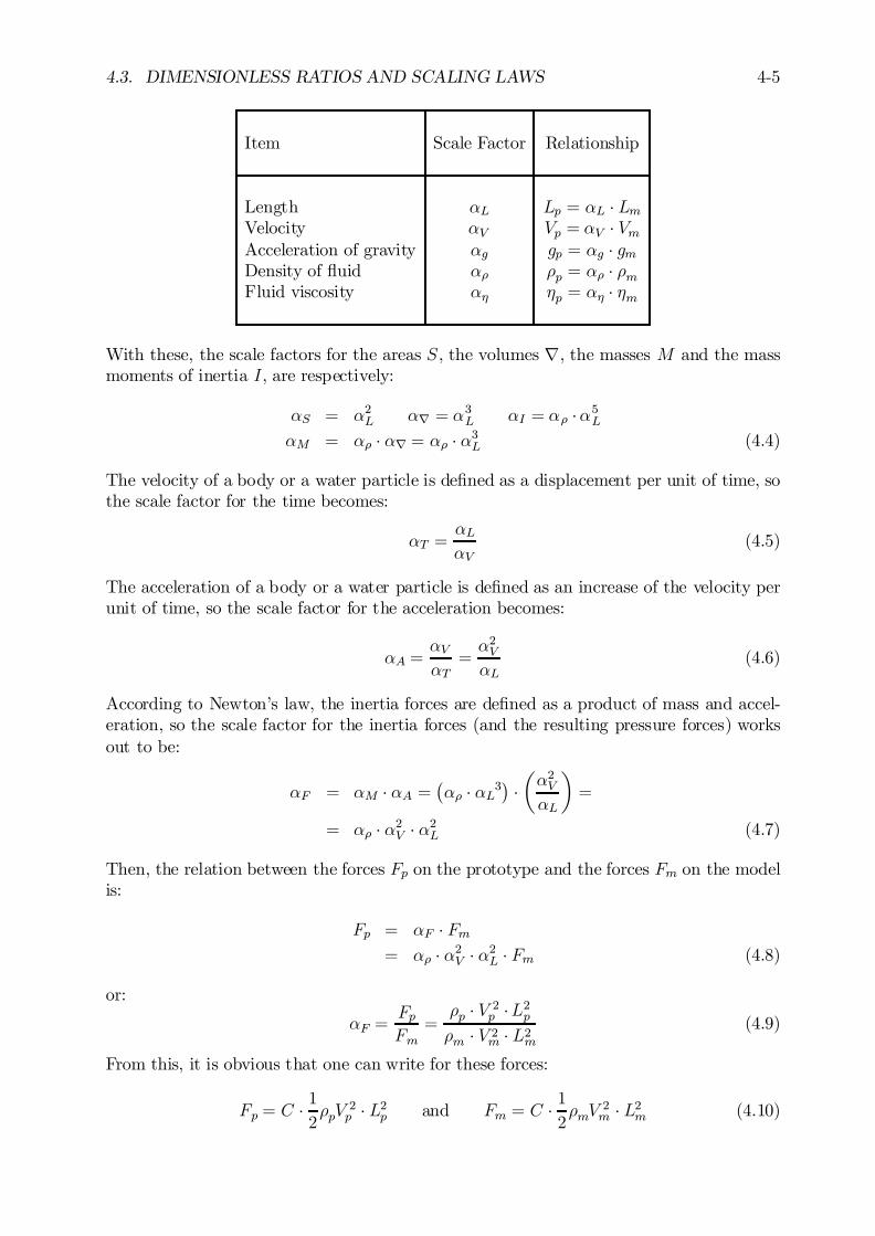
4.3. DIMENSIONLESS RATIOS AND SCALING LAWS 4-5
Item Scale Factor Relationship
Length ®L Lp = ®L ¢ LmVelocity ®V Vp = ®V ¢ VmAcceleration of gravity ®g gp = ®g ¢ gmDensity of ‡uid ®½ ½p = ®½ ¢ ½mFluid viscosity ®´ ´p = ®´ ¢ ´m
With these, the scale factors for the areas S , the volumes r, the masses M and the massmoments of inertia I, are respectively:
®S = ®2L ®r = ®3L ®I = ®½ ¢®5L
®M = ®½ ¢ ®r = ®½ ¢ ®3L (4.4)
The velocity of a body or a water particle is de…ned as a displacement per unit of time, sothe scale factor for the time becomes:
®T =®L®V
(4.5)
The acceleration of a body or a water particle is de…ned as an increase of the velocity perunit of time, so the scale factor for the acceleration becomes:
®A =®V®T
=®2V®L
(4.6)
According to Newton’s law, the inertia forces are de…ned as a product of mass and accel-eration, so the scale factor for the inertia forces (and the resulting pressure forces) worksout to be:
®F = ®M ¢ ®A =¡®½ ¢ ®L3
¢¢µ®2V®L
¶=
= ®½ ¢ ®2V ¢ ®2L (4.7)
Then, the relation between the forces Fp on the prototype and the forces Fm on the modelis:
Fp = ®F ¢ Fm= ®½ ¢ ®2V ¢ ®2L ¢ Fm (4.8)
or:
®F =FpFm
=½p ¢ V 2p ¢L2p½m ¢ V 2m ¢ L2m
(4.9)
From this, it is obvious that one can write for these forces:
Fp = C ¢ 12½pV
2p ¢ L2p and Fm = C ¢ 1
2½mV
2m ¢ L2m (4.10)
4-6 CHAPTER 4. CONSTANT REAL FLOW PHENOMENA
in which the constant coe¢cient, C, does not depend on the scale of the model nor on thestagnation pressure term 1
2½V2.
Viscous forces can be expressed using Newton’s friction model as being proportional to:
Fv ® ´V
LL2 (4.11)
while the inertia forces (from above) are proportional to:
Fi ® ½L3V 2
L= ½L2V 2 (4.12)
The ratio of these two forces is then - after cancelling out some terms:
FiFv=½
´V ¢ L = V ¢ L
º= Rn (4.13)
The Reynolds number is thus a measure of the ratio of these forces. Viscous forces arepredominant when the Reynolds number is small.Gravity forces are simply proportional to the material density, the acceleration of gravityand the volume:
Fg ® ½gL3 (4.14)
The above information can be used to help design physical models. One can deduce thatvarious forces are represented to di¤erent scales. It is therefore impossible to represent allmodel forces with the same relative importance as in the prototype. A choice is thereforeoften made, instead, to maintain the ratio between the two most important forces in theprototype when a physical model is built. This can result in several scaling laws as outlinedin appendix B. Two of the more important forms are discussed here, however.
4.3.2 Reynolds Scaling
Reynolds scaling is used when inertia and viscous forces are of predominant importancein the ‡ow. This is the case for pipe ‡ow (under pressure) and for wake formation behinda body in a ‡ow. Reynolds scaling requires that the Reynolds number in the model beidentical to that in the prototype. Using the basic relations above:
VmLmºm
=VpLpºp
(4.15)
or, expressed another way:®V ¢ ®L®º
= 1: (4.16)
Since ®V = ®L=®T , then this becomes:
®T =®2L®º
(4.17)
Since the ‡uids in the model and in the ocean are about the same, ®º (and even ®½ forthat matter) is very close to 1.0, so that:
®T t ®2L (4.18)
4.3. DIMENSIONLESS RATIOS AND SCALING LAWS 4-7
This last result, that the time scale is the square of the length scale, would mean that timewould pass quite rapidly in the model. Also, one can make further substitutions to discoverthat ®F is equal to unity; forces in the model would be just as big as in the prototype -again very impractical!
4.3.3 Froude Scaling
Gravity forces become important when a free surface of a liquid is involved. This will betrue, whenever a water surface or waves are present. Since inertia and pressure forces arenearly universally important, this makes it appropriate to keep the ratio of inertia or pressure forces
gravity forcesthe same in the model as in the prototype. Scaling based upon the square root of this ra-tio is called Froude scaling, after Robert Edmund Froude (as distinct from his fatherWilliam Froude from the model resistance extrapolation to full scale, treated in a followingsection) who has …rst used it.Working this out from the basic information above and in a way very analogous to thatused for Reynolds scaling yields:
Fn =
sinertia or pressure forces
gravity forces
=
s®½ ¢ ®2V ¢ ®2L®½ ¢ ®3L ¢ ®g
=®Vp®g ¢ ®L
=VpgL
(4.19)
Since it is especially di¢cult (or at least very costly) to change the acceleration of gravityfor a model involving free liquid surfaces, one may safely set ®g = 1. Continuing as wasdone above, one …nds that:
®T =p®L (4.20)
This is a lot more convenient to handle than Reynolds scaling!
4.3.4 Numerical Example
As an example, suppose a ship with a length Ls = Lpp = 100 meter, which sails with aforward ship speed V of 20 knots in still seawater with a temperature of 15±C. Resistanceand propulsion tests will be carried out in a towing tank with a 1:40 scale physical model(®L = 40). The temperature of the fresh water in the tank is 20oC.The density and the kinematic viscosity of fresh water, salt water and dry air as a function ofthe temperature are listed in appendix A. Values needed here are for sea water: ½ = 1025:9kg/m3 and º = 1:19 ¢ 10¡6 m2/s. The relevant values for fresh water are now: ½ = 998:1kg/m3 and º = 1:05 ¢ 10¡6 m2/s.The length of the ship model is:
Lm =Ls®L=100
40= 2:50 m (4.21)
The speed Vs of the ship is:
Vs = 0:5144 ¢ V = 0:5144 ¢ 20 = 10:29 m/s (4.22)
4-8 CHAPTER 4. CONSTANT REAL FLOW PHENOMENA
For practical reasons, the speed of the model will be obtained using Froude scaling:
Vm =Vsp®L=10:29p40
= 1:63 m/s (4.23)
As a consequence, the Froude numbers for the ship and model are obviously identical andequal to 0:329:A consequence of this scaling is that the Reynolds numbers will di¤er:
Rns =Vs ¢ Lsºsalt
=10:29 ¢ 1001:19 ¢ 10¡6 = 865 ¢ 106
Rnm =Vm ¢ Lmºfresh
=1:63 ¢ 2:501:05 ¢ 10¡6 = 3:88 ¢ 106 (4.24)
so that:
®Rn = 223 (4.25)
In order to obtain equal Reynolds numbers, the ”model water” needs a kinematic viscositywhich is 1/223 times its actual value; this liquid is not available!
Reynolds versus Froude scaling will be picked up again later in this chapter. First, however,the next sections of this chapter will discuss the ‡ow around and hydrodynamic forces ona slender cylinder in a constant current.
4.4 Cylinder Flow Regimes
This …gure below summarizes the various forms of ‡ow around a cylinder. A more completediscussion can be found in [Schlichting, 1951]. The Reynolds number (listed on the left,below the ‡ow pattern name) is used in …gure 4.3 to characterize each type of ‡ow. Thesigni…cance of the Cd values listed there will become clear in a later section of this chapter,by the way. The right hand column in …gure 4.3 gives a short comparative description ofthe ‡ow pattern.
4.5 Drag and Lift
Now that the ‡ow patterns near a circular cylinder have been determined, attention canbe shifted to the forces that result from the ‡ow.
4.5.1 Drag Force and Drag Coe¢cient
The pressure variation near a cylinder wall was given in chapter 3. Applying this now ina slightly di¤erent way to reveal the pressure di¤erence, relative to an undisturbed ‡owpressure, yields:
¢p = p ¡ p0=
1
2¢ ½ ¢ U 21 ¢
¡1¡ 4 ¢ sin2µ
¢(4.26)
in which:

4.5. DRAG AND LIFT 4-9
Figure 4.3: Flow Regiems and Descriptions
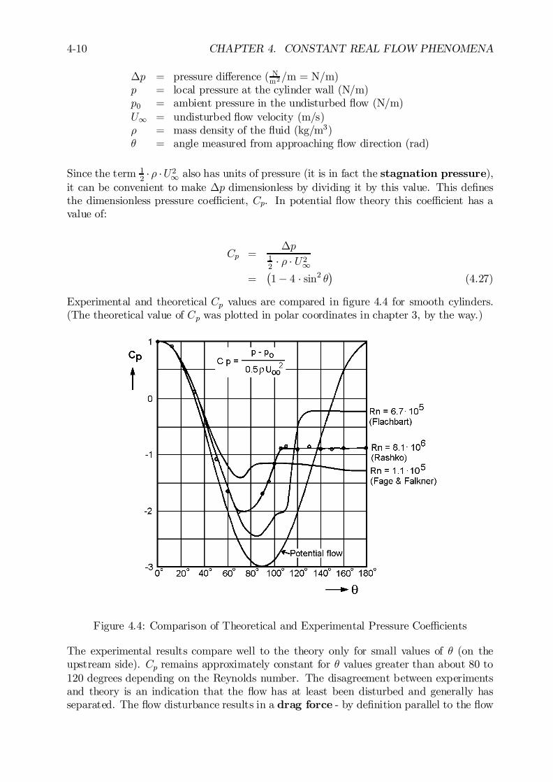
4-10 CHAPTER 4. CONSTANT REAL FLOW PHENOMENA
¢p = pressure di¤erence ( Nm2/m = N/m)
p = local pressure at the cylinder wall (N/m)p0 = ambient pressure in the undisturbed ‡ow (N/m)U1 = undisturbed ‡ow velocity (m/s)½ = mass density of the ‡uid (kg/m3)µ = angle measured from approaching ‡ow direction (rad)
Since the term 12¢ ½ ¢U21 also has units of pressure (it is in fact the stagnation pressure),
it can be convenient to make ¢p dimensionless by dividing it by this value. This de…nesthe dimensionless pressure coe¢cient, Cp. In potential ‡ow theory this coe¢cient has avalue of:
Cp =¢p
12
¢ ½ ¢ U21=
¡1¡ 4 ¢ sin2 µ
¢(4.27)
Experimental and theoretical Cp values are compared in …gure 4.4 for smooth cylinders.(The theoretical value of Cp was plotted in polar coordinates in chapter 3, by the way.)
Figure 4.4: Comparison of Theoretical and Experimental Pressure Coe¢cients
The experimental results compare well to the theory only for small values of µ (on theupstream side). Cp remains approximately constant for µ values greater than about 80 to120 degrees depending on the Reynolds number. The disagreement between experimentsand theory is an indication that the ‡ow has at least been disturbed and generally hasseparated. The ‡ow disturbance results in a drag force - by de…nition parallel to the ‡ow
4.5. DRAG AND LIFT 4-11
direction - on the cylinder. This force (on a unit length of cylinder) can be written as afunction of the (undisturbed) stagnation pressure:
FD =1
2½ U2 CDD (4.28)
in which:
FD = drag force per unit length of cylinder (N/m)½ = mass density of the ‡uid (kg/m3)CD = dimensionless coe¢cient (-)D = cylinder diameter (m)U = undisturbed ‡ow velocity (m/s)
The drag force is the product of the stagnation pressure, 12 ½ U2; an area, D times a unit
length, and a dimensionless coe¢cient, CD:This equation thus de…nes the drag coe¢cient as:
CD =FD
12½ U2 ¢D (4.29)
The drag coe¢cient depends on Rn, the cylinder’s roughness and the turbulence of theincident ‡ow. The resulting drag coe¢cients for a …xed smooth cylinder in a constantvelocity ‡ow have already been included in …gure 4.3.
Fall Velocity
One of the simplest applications of the drag force concept is for the determination of thefall velocity of an object. This is the maximum speed with which an object will fall throughthe medium which surrounds it. A parachute jumper soon reaches his or her fall velocity(of about 7 m/s) after jumping out of an aircraft, for example. Attention in o¤shoreengineering focuses instead on the speed at which sand grains or gravel or even ropes andchains fall through sea water.The fall velocity in any of these cases is determined by an equilibrium between thesubmerged weight (see chapter 2) of the object on the one hand and the drag forcefrom its environment on the other. In equation form:
Wsub = CDD ¢ 12½ Vf
2 (4.30)
in which Wsub is the submerged weight of the object (N) and Vf is the fall velocity of theobject (m/s).If one is considering an isolated particle - such as a stone, then the drag coe¢cient, CD ;usedin equation 4.30 will be for the three-dimensional object. If, on the other hand, a longobject such as a rope (fall crosswise) is being considered, then Wsub and CD relate to thetwo dimensional object.CD in equation 4.30 is dependent upon the Reynolds number which depends in turn uponthe velocity, Vf . One must iterate (a simple trial-and-error approach is sophisticatedenough) to …nd the proper combination of these two unknowns. This is illustrated herefor a steel wire rope such as is used as the main tow rope on the Smit Rotterdam, one of
4-12 CHAPTER 4. CONSTANT REAL FLOW PHENOMENA
the largest tugboats in the world. The basic data is that the segment of wire rope is 3inches (76 mm) in diameter and has a submerged weight of 196 N/m. Because the surfaceof the rope is rough, (it is made from twisted strands of wire) it will have a drag coe¢cientwhich is about 30% higher than that listed above for a smooth cylinder. The iteration isindicated in the following table.
Vf guess Rn CD Vf calc
(m/s) (-) (-) (m/s)
5.0 375 000 1.2 2.052.0 150 000 1.6 1.781.78 131 250 1.6 1.78
The computation converges quite easily. The numerical value may surprise some; even aseemingly heavy steel wire rope will not fall all that fast in water!The order of magnitude of the fall velocities for other materials is summarized in the tablebelow.
Quantity! D Wsub Rn Vf(mm) (N) (-) (m/s)
Object #
sand grain 0.2 0.07¢10¡6 ¼2 0.02gravel 20 0.07 20 000 1.00stone 100 8.38 235 000 2.351 m wire rope 76 196 131 250 1.781 m chain 76 1079 396000 3.00
Common Fall Velocities
This data for sand, gravel and stones will be handy later when sea bed morphology isdiscussed in chapter 14. The diameter used for chain is based upon its mass per unitlength. Its drag coe¢cient is about 50% higher than that of a smooth cylinder.Of course some objects can fall much faster than the values given here. A 400 ton pilewas dropped by accident in the Gulf of Mexico when it was hanging in a vertical position.A crude under water measurement, made before it would have reached its terminal fallvelocity, indicated a speed of about 11 m/s. When it hit the sea bed - luckily next to theplatform it was originally intended for - its impact caused it to penetrate 75 meters intothe sea bed.
4.5.2 Lift Force and Strouhal Number
A lift force is de…ned as a force component acting perpendicular to the undisturbed ‡owvelocity. It is therefore also perpendicular to the drag force component. As explained
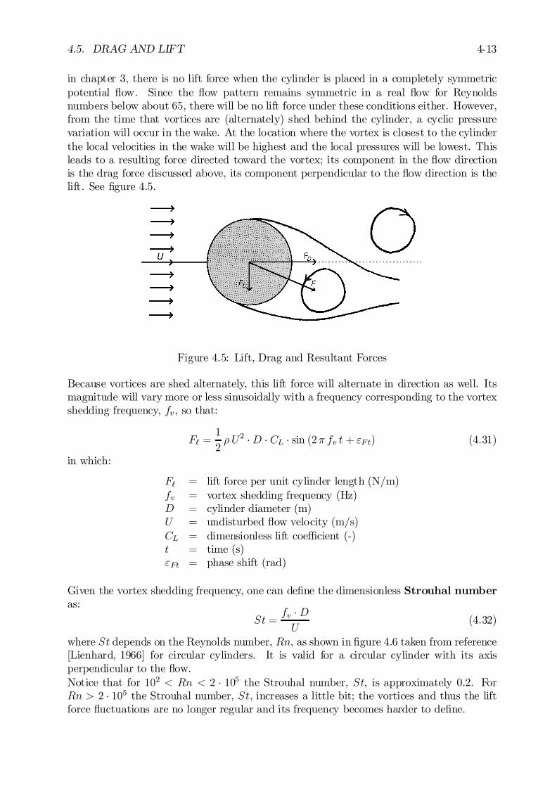
4.5. DRAG AND LIFT 4-13
in chapter 3, there is no lift force when the cylinder is placed in a completely symmetricpotential ‡ow. Since the ‡ow pattern remains symmetric in a real ‡ow for Reynoldsnumbers below about 65, there will be no lift force under these conditions either. However,from the time that vortices are (alternately) shed behind the cylinder, a cyclic pressurevariation will occur in the wake. At the location where the vortex is closest to the cylinderthe local velocities in the wake will be highest and the local pressures will be lowest. Thisleads to a resulting force directed toward the vortex; its component in the ‡ow directionis the drag force discussed above, its component perpendicular to the ‡ow direction is thelift. See …gure 4.5.
Figure 4.5: Lift, Drag and Resultant Forces
Because vortices are shed alternately, this lift force will alternate in direction as well. Itsmagnitude will vary more or less sinusoidally with a frequency corresponding to the vortexshedding frequency, fv, so that:
F` =1
2½ U2 ¢D ¢ CL ¢ sin (2¼ fv t + "Ft) (4.31)
in which:
F` = lift force per unit cylinder length (N/m)fv = vortex shedding frequency (Hz)D = cylinder diameter (m)U = undisturbed ‡ow velocity (m/s)CL = dimensionless lift coe¢cient (-)t = time (s)"Ft = phase shift (rad)
Given the vortex shedding frequency, one can de…ne the dimensionless Strouhal numberas:
St =fv ¢DU
(4.32)
where St depends on the Reynolds number, Rn, as shown in …gure 4.6 taken from reference[Lienhard, 1966] for circular cylinders. It is valid for a circular cylinder with its axisperpendicular to the ‡ow.Notice that for 102 < Rn < 2 ¢ 105 the Strouhal number, St, is approximately 0.2. ForRn > 2 ¢ 105 the Strouhal number, St, increases a little bit; the vortices and thus the liftforce ‡uctuations are no longer regular and its frequency becomes harder to de…ne.
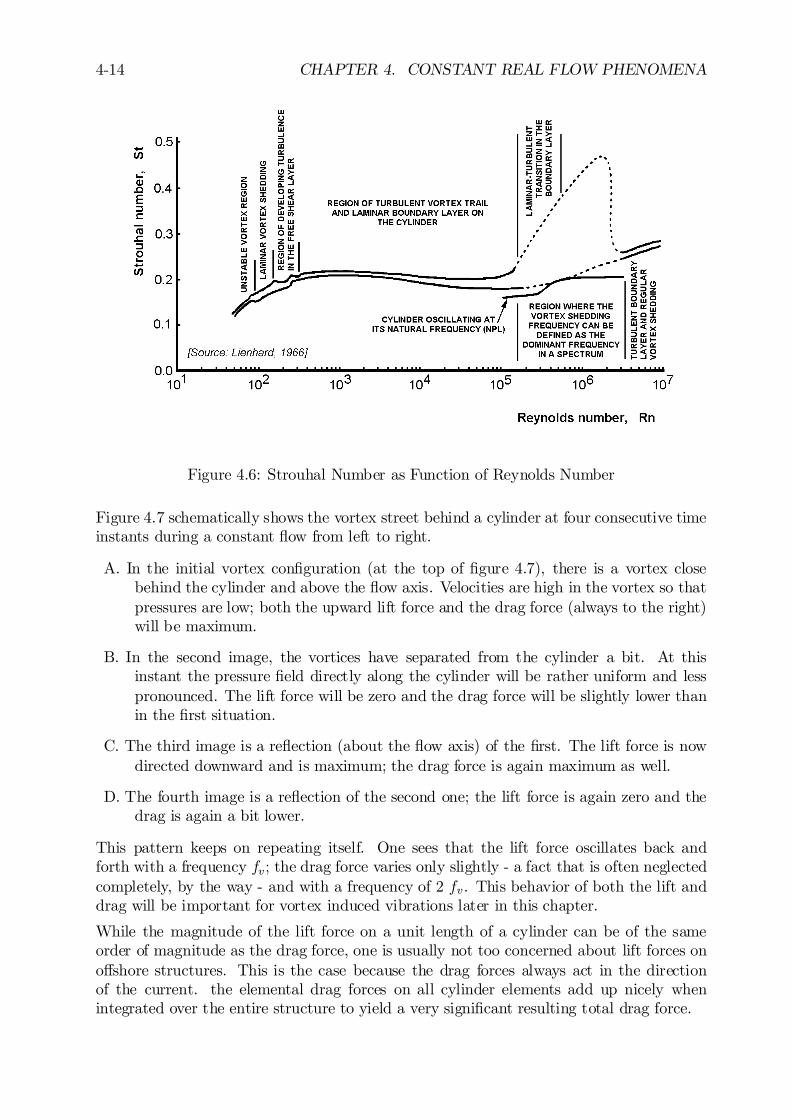
4-14 CHAPTER 4. CONSTANT REAL FLOW PHENOMENA
Figure 4.6: Strouhal Number as Function of Reynolds Number
Figure 4.7 schematically shows the vortex street behind a cylinder at four consecutive timeinstants during a constant ‡ow from left to right.
A. In the initial vortex con…guration (at the top of …gure 4.7), there is a vortex closebehind the cylinder and above the ‡ow axis. Velocities are high in the vortex so thatpressures are low; both the upward lift force and the drag force (always to the right)will be maximum.
B. In the second image, the vortices have separated from the cylinder a bit. At thisinstant the pressure …eld directly along the cylinder will be rather uniform and lesspronounced. The lift force will be zero and the drag force will be slightly lower thanin the …rst situation.
C. The third image is a re‡ection (about the ‡ow axis) of the …rst. The lift force is nowdirected downward and is maximum; the drag force is again maximum as well.
D. The fourth image is a re‡ection of the second one; the lift force is again zero and thedrag is again a bit lower.
This pattern keeps on repeating itself. One sees that the lift force oscillates back andforth with a frequency fv ; the drag force varies only slightly - a fact that is often neglectedcompletely, by the way - and with a frequency of 2 fv. This behavior of both the lift anddrag will be important for vortex induced vibrations later in this chapter.
While the magnitude of the lift force on a unit length of a cylinder can be of the sameorder of magnitude as the drag force, one is usually not too concerned about lift forces ono¤shore structures. This is the case because the drag forces always act in the directionof the current. the elemental drag forces on all cylinder elements add up nicely whenintegrated over the entire structure to yield a very signi…cant resulting total drag force.
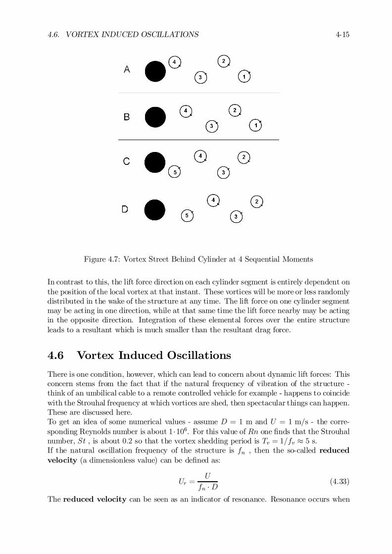
4.6. VORTEX INDUCED OSCILLATIONS 4-15
Figure 4.7: Vortex Street Behind Cylinder at 4 Sequential Moments
In contrast to this, the lift force direction on each cylinder segment is entirely dependent onthe position of the local vortex at that instant. These vortices will be more or less randomlydistributed in the wake of the structure at any time. The lift force on one cylinder segmentmay be acting in one direction, while at that same time the lift force nearby may be actingin the opposite direction. Integration of these elemental forces over the entire structureleads to a resultant which is much smaller than the resultant drag force.
4.6 Vortex Induced Oscillations
There is one condition, however, which can lead to concern about dynamic lift forces: Thisconcern stems from the fact that if the natural frequency of vibration of the structure -think of an umbilical cable to a remote controlled vehicle for example - happens to coincidewith the Strouhal frequency at which vortices are shed, then spectacular things can happen.These are discussed here.To get an idea of some numerical values - assume D = 1 m and U = 1 m/s - the corre-sponding Reynolds number is about 1¢106. For this value of Rn one …nds that the Strouhalnumber, St , is about 0:2 so that the vortex shedding period is Tv = 1=fv ¼ 5 s.If the natural oscillation frequency of the structure is fn , then the so-called reducedvelocity (a dimensionless value) can be de…ned as:
Ur =U
fn ¢D (4.33)
The reduced velocity can be seen as an indicator of resonance. Resonance occurs when
4-16 CHAPTER 4. CONSTANT REAL FLOW PHENOMENA
the vortex shedding frequency fv approaches the natural frequency, fn:
fv =St ¢ UD
! fn (4.34)
so that the reduced velocity is then approximately:
Ur =1
St¼ 5 (4.35)
Thus, once the natural oscillation frequency of a structure (long risers, or umbilical cablesare …ne examples) is known, one can determine Ur and use it to predict a danger fromresonant vortex-induced oscillations.
4.6.1 Crosswise Oscillations
To understand what is happening, consider the situation as one slowly increases the ‡owvelocity, U , past a cylinder. When the velocity is low enough (but still high enough tocause alternating vortex shedding), the cylinder will remain relatively still in the ‡ow andthe vortices will be randomly distributed along the cylinder length in its wake. As Uincreases, fv will increase too. As Ur approaches a value of about 5 one observes that thecylinder begins to oscillate signi…cantly in a direction crosswise to the ‡ow. A signi…cante¤ect of this cylinder oscillation is that it distorts the local ‡ow pattern, making it moreattractive for vortices to be shed ’behind’ the cylinder (seen from the perspective of boththe cylinder motion and the ‡ow). Since each adjacent segment of the cylinder is movingin more or less the same way at any instant in time, this in turn stimulates the vortices tobecome more coherent along the cylinder length. The more or less randomly distributedlift forces on di¤erent cylinder or cable segments now start working in phase with oneanother. The cable responds to this more coherent lift force excitation by oscillating witha larger amplitude - thus reinforcing the entire process; this is called lock-in.As the ambient ‡ow velocity continues to increase, lock-in will ultimately stop (usuallyafter Ur reaches a value of about 7) and the cable comes more or less to rest again. Peopleare still trying to explain and accurately predict these phenomena.
In‡uence on Drag
A secondary e¤ect of transverse cylinder oscillations can be an increased drag force. Thereare two ”popular and pragmatic” approaches to explain this.Remembering …rst that the drag force is:
FD =1
2½ U2 ¢ CD ¢D (4.36)
Then:
² Because the cylinder is oscillating (crosswise to the ‡ow), its wake becomes wider.This has an e¤ect similar to that of increasing D; which would increase FD. This isusually expressed by increasing the value of CD , instead..
² Since the cylinder now also moves with speed dY=dt, the instantaneous incident ‡owvelocity relative to cylinder becomes:
~Ui = ¡dYdt~y + U ~x (4.37)
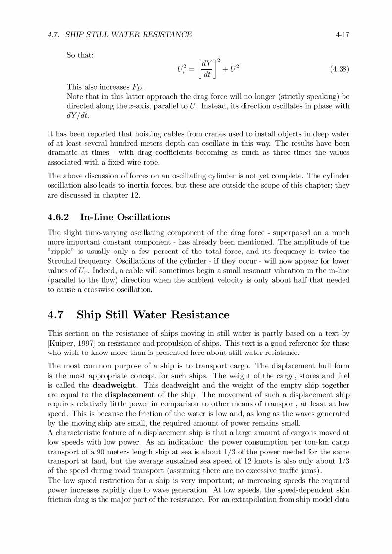
4.7. SHIP STILL WATER RESISTANCE 4-17
So that:
U2i =
·dY
dt
¸2+ U2 (4.38)
This also increases FD.Note that in this latter approach the drag force will no longer (strictly speaking) bedirected along the x-axis, parallel to U . Instead, its direction oscillates in phase withdY=dt.
It has been reported that hoisting cables from cranes used to install objects in deep waterof at least several hundred meters depth can oscillate in this way. The results have beendramatic at times - with drag coe¢cients becoming as much as three times the valuesassociated with a …xed wire rope.
The above discussion of forces on an oscillating cylinder is not yet complete. The cylinderoscillation also leads to inertia forces, but these are outside the scope of this chapter; theyare discussed in chapter 12.
4.6.2 In-Line Oscillations
The slight time-varying oscillating component of the drag force - superposed on a muchmore important constant component - has already been mentioned. The amplitude of the”ripple” is usually only a few percent of the total force, and its frequency is twice theStrouhal frequency. Oscillations of the cylinder - if they occur - will now appear for lowervalues of Ur. Indeed, a cable will sometimes begin a small resonant vibration in the in-line(parallel to the ‡ow) direction when the ambient velocity is only about half that neededto cause a crosswise oscillation.
4.7 Ship Still Water Resistance
This section on the resistance of ships moving in still water is partly based on a text by[Kuiper, 1997] on resistance and propulsion of ships. This text is a good reference for thosewho wish to know more than is presented here about still water resistance.
The most common purpose of a ship is to transport cargo. The displacement hull formis the most appropriate concept for such ships. The weight of the cargo, stores and fuelis called the deadweight. This deadweight and the weight of the empty ship togetherare equal to the displacement of the ship. The movement of such a displacement shiprequires relatively little power in comparison to other means of transport, at least at lowspeed. This is because the friction of the water is low and, as long as the waves generatedby the moving ship are small, the required amount of power remains small.A characteristic feature of a displacement ship is that a large amount of cargo is moved atlow speeds with low power. As an indication: the power consumption per ton-km cargotransport of a 90 meters length ship at sea is about 1/3 of the power needed for the sametransport at land, but the average sustained sea speed of 12 knots is also only about 1/3of the speed during road transport (assuming there are no excessive tra¢c jams).The low speed restriction for a ship is very important; at increasing speeds the requiredpower increases rapidly due to wave generation. At low speeds, the speed-dependent skinfriction drag is the major part of the resistance. For an extrapolation from ship model data
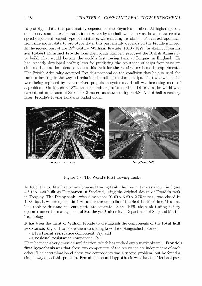
4-18 CHAPTER 4. CONSTANT REAL FLOW PHENOMENA
to prototype data, this part mainly depends on the Reynolds number. At higher speeds,one observes an increasing radiation of waves by the hull, which means the appearance of aspeed-dependent second type of resistance; wave making resistance. For an extrapolationfrom ship model data to prototype data, this part mainly depends on the Froude number.In the second part of the 19th century William Froude, 1810 - 1879, (as distinct from hisson Robert Edmund Froude from the Froude number) proposed the British Admiraltyto build what would become the world’s …rst towing tank at Torquay in England. Hehad recently developed scaling laws for predicting the resistance of ships from tests onship models and he intended to use this tank for the required scale model experiments.The British Admiralty accepted Froude’s proposal on the condition that he also used thetank to investigate the ways of reducing the rolling motion of ships. That was when sailswere being replaced by steam driven propulsion systems and roll was becoming more ofa problem. On March 3 1872, the …rst indoor professional model test in the world wascarried out in a basin of 85 x 11 x 3 meter, as shown in …gure 4.8. About half a centurylater, Froude’s towing tank was pulled down.
Figure 4.8: The World’s First Towing Tanks
In 1883, the world’s …rst privately owned towing tank, the Denny tank as shown in …gure4.8 too, was built at Dumbarton in Scotland, using the original design of Froude’s tankin Torquay. The Denny tank - with dimensions 93.00 x 6.80 x 2.75 meter - was closed in1983, but it was re-opened in 1986 under the umbrella of the Scottish Maritime Museum.The tank testing and museum parts are separate. Since 1989, the tank testing facilityoperates under the management of Strathclyde University’s Department of Ship and MarineTechnology.
It has been the merit of William Froude to distinguish the components of the total hullresistance, Rt, and to relate them to scaling laws; he distinguished between:
- a frictional resistance component, Rf, and- a residual resistance component, Rr .
Then he made a very drastic simpli…cation, which has worked out remarkably well: Froude’s…rst hypothesis was that these two components of the resistance are independent of eachother. The determination of these two components was a second problem, but he found asimple way out of this problem. Froude’s second hypothesis was that the frictional part
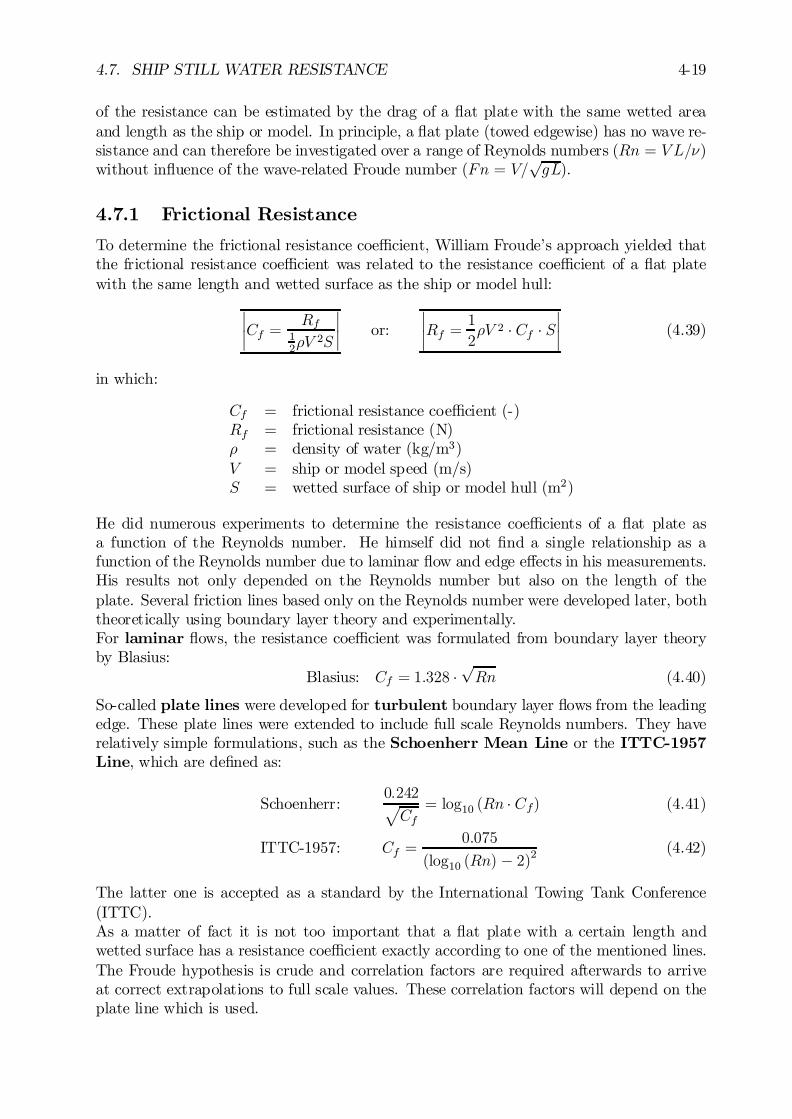
4.7. SHIP STILL WATER RESISTANCE 4-19
of the resistance can be estimated by the drag of a ‡at plate with the same wetted areaand length as the ship or model. In principle, a ‡at plate (towed edgewise) has no wave re-sistance and can therefore be investigated over a range of Reynolds numbers (Rn = VL=º)without in‡uence of the wave-related Froude number (Fn = V=
pgL).
4.7.1 Frictional Resistance
To determine the frictional resistance coe¢cient, William Froude’s approach yielded thatthe frictional resistance coe¢cient was related to the resistance coe¢cient of a ‡at platewith the same length and wetted surface as the ship or model hull:
¯¯Cf =
Rf12½V
2S
¯¯ or:
¯¯Rf =
1
2½V 2 ¢ Cf ¢ S
¯¯ (4.39)
in which:
Cf = frictional resistance coe¢cient (-)Rf = frictional resistance (N)½ = density of water (kg/m3)V = ship or model speed (m/s)S = wetted surface of ship or model hull (m2)
He did numerous experiments to determine the resistance coe¢cients of a ‡at plate asa function of the Reynolds number. He himself did not …nd a single relationship as afunction of the Reynolds number due to laminar ‡ow and edge e¤ects in his measurements.His results not only depended on the Reynolds number but also on the length of theplate. Several friction lines based only on the Reynolds number were developed later, boththeoretically using boundary layer theory and experimentally.For laminar ‡ows, the resistance coe¢cient was formulated from boundary layer theoryby Blasius:
Blasius: Cf = 1:328 ¢pRn (4.40)
So-called plate lines were developed for turbulent boundary layer ‡ows from the leadingedge. These plate lines were extended to include full scale Reynolds numbers. They haverelatively simple formulations, such as the Schoenherr Mean Line or the ITTC-1957Line, which are de…ned as:
Schoenherr:0:242pCf
= log10 (Rn ¢ Cf) (4.41)
ITTC-1957: Cf =0:075
(log10 (Rn) ¡ 2)2(4.42)
The latter one is accepted as a standard by the International Towing Tank Conference(ITTC).As a matter of fact it is not too important that a ‡at plate with a certain length andwetted surface has a resistance coe¢cient exactly according to one of the mentioned lines.The Froude hypothesis is crude and correlation factors are required afterwards to arriveat correct extrapolations to full scale values. These correlation factors will depend on theplate line which is used.

4-20 CHAPTER 4. CONSTANT REAL FLOW PHENOMENA
4.7.2 Residual Resistance
The determination of the resistance components of a ship’s hull can be illustrated with theresults of resistance tests with a series of models at various scales, the ”Simon Bolivar”family of models. Resistance tests were carried out over a certain speed range for eachof the models. Each model had a di¤erent scale factor, ®. The total resistance (in non-dimensional form) is shown in …gure 4.9.
Figure 4.9: Resistance Coe¢cients of the ”Simon Bolivar” Model Family
The total resistance force on a ship is made non-dimensional in the same way as thefrictional resistance above:
¯¯Ct =
Rt12½V
2S
¯¯ or:
¯¯Rt =
1
2½V 2 ¢ Ct ¢ S
¯¯ (4.43)
in which:
Ct = total resistance coe¢cient (-)Rt = total resistance (N)½ = density of water (kg/m3)V = ship or model speed (m/s)S = wetted surface of ship or model hull (m2)
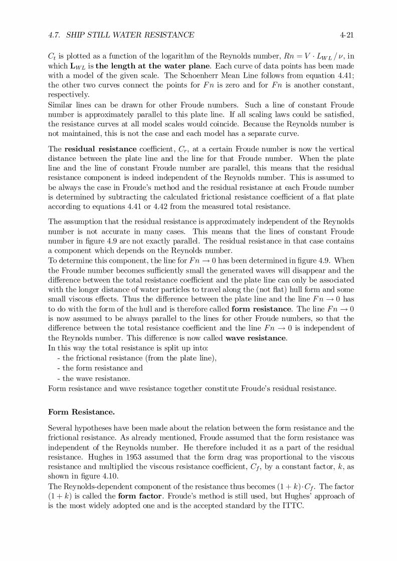
4.7. SHIP STILL WATER RESISTANCE 4-21
Ct is plotted as a function of the logarithm of the Reynolds number, Rn = V ¢ LWL =º, inwhich LWL is the length at the water plane. Each curve of data points has been madewith a model of the given scale. The Schoenherr Mean Line follows from equation 4.41;the other two curves connect the points for Fn is zero and for Fn is another constant,respectively.Similar lines can be drawn for other Froude numbers. Such a line of constant Froudenumber is approximately parallel to this plate line. If all scaling laws could be satis…ed,the resistance curves at all model scales would coincide. Because the Reynolds number isnot maintained, this is not the case and each model has a separate curve.
The residual resistance coe¢cient, Cr, at a certain Froude number is now the verticaldistance between the plate line and the line for that Froude number. When the plateline and the line of constant Froude number are parallel, this means that the residualresistance component is indeed independent of the Reynolds number. This is assumed tobe always the case in Froude’s method and the residual resistance at each Froude numberis determined by subtracting the calculated frictional resistance coe¢cient of a ‡at plateaccording to equations 4.41 or 4.42 from the measured total resistance.
The assumption that the residual resistance is approximately independent of the Reynoldsnumber is not accurate in many cases. This means that the lines of constant Froudenumber in …gure 4.9 are not exactly parallel. The residual resistance in that case containsa component which depends on the Reynolds number.To determine this component, the line for Fn ! 0 has been determined in …gure 4.9. Whenthe Froude number becomes su¢ciently small the generated waves will disappear and thedi¤erence between the total resistance coe¢cient and the plate line can only be associatedwith the longer distance of water particles to travel along the (not ‡at) hull form and somesmall viscous e¤ects. Thus the di¤erence between the plate line and the line Fn ! 0 hasto do with the form of the hull and is therefore called form resistance. The line Fn ! 0is now assumed to be always parallel to the lines for other Froude numbers, so that thedi¤erence between the total resistance coe¢cient and the line Fn ! 0 is independent ofthe Reynolds number. This di¤erence is now called wave resistance.In this way the total resistance is split up into:
- the frictional resistance (from the plate line),- the form resistance and- the wave resistance.
Form resistance and wave resistance together constitute Froude’s residual resistance.
Form Resistance.
Several hypotheses have been made about the relation between the form resistance and thefrictional resistance. As already mentioned, Froude assumed that the form resistance wasindependent of the Reynolds number. He therefore included it as a part of the residualresistance. Hughes in 1953 assumed that the form drag was proportional to the viscousresistance and multiplied the viscous resistance coe¢cient, Cf , by a constant factor, k, asshown in …gure 4.10.The Reynolds-dependent component of the resistance thus becomes (1 + k)¢Cf . The factor(1 + k) is called the form factor. Froude’s method is still used, but Hughes’ approach ofis the most widely adopted one and is the accepted standard by the ITTC.
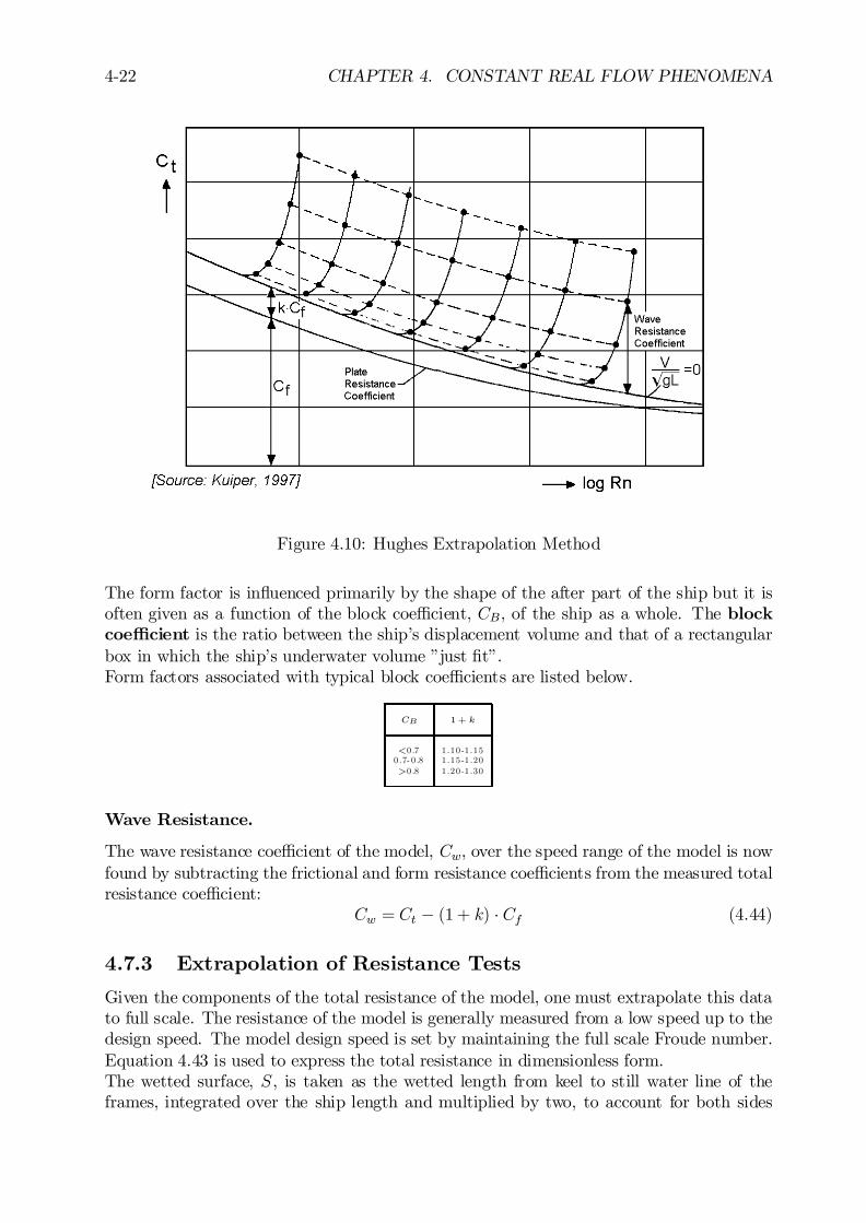
4-22 CHAPTER 4. CONSTANT REAL FLOW PHENOMENA
Figure 4.10: Hughes Extrapolation Method
The form factor is in‡uenced primarily by the shape of the after part of the ship but it isoften given as a function of the block coe¢cient, CB, of the ship as a whole. The blockcoe¢cient is the ratio between the ship’s displacement volume and that of a rectangularbox in which the ship’s underwater volume ”just …t”.Form factors associated with typical block coe¢cients are listed below.
CB 1 + k
<0 .7 1 .10 -1 .150 .7- 0 .8 1 .15 -1 .20>0 .8 1 .20 -1 .30
Wave Resistance.
The wave resistance coe¢cient of the model, Cw, over the speed range of the model is nowfound by subtracting the frictional and form resistance coe¢cients from the measured totalresistance coe¢cient:
Cw = Ct ¡ (1 + k) ¢ Cf (4.44)
4.7.3 Extrapolation of Resistance Tests
Given the components of the total resistance of the model, one must extrapolate this datato full scale. The resistance of the model is generally measured from a low speed up to thedesign speed. The model design speed is set by maintaining the full scale Froude number.Equation 4.43 is used to express the total resistance in dimensionless form.The wetted surface, S , is taken as the wetted length from keel to still water line of theframes, integrated over the ship length and multiplied by two, to account for both sides
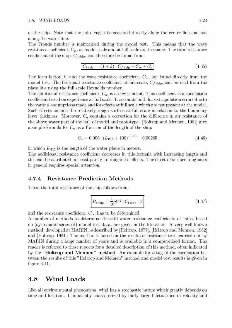
4.8. WIND LOADS 4-23
of the ship. Note that the ship length is measured directly along the center line and notalong the water line.The Froude number is maintained during the model test. This means that the waveresistance coe¢cient, Cw , at model scale and at full scale are the same. The total resistancecoe¢cient of the ship, Ct ship, can therefore be found from:
jCt ship = (1 + k) ¢ Cf ship +Cw+ Caj (4.45)
The form factor, k, and the wave resistance coe¢cient, Cw , are found directly from themodel test. The frictional resistance coe¢cient at full scale, Cf ship, can be read from theplate line using the full scale Reynolds number.The additional resistance coe¢cient, Ca, is a new element. This coe¢cient is a correlationcoe¢cient based on experience at full scale. It accounts both for extrapolation errors due tothe various assumptions made and for e¤ects at full scale which are not present at the model.Such e¤ects include the relatively rough surface at full scale in relation to the boundarylayer thickness. Moreover, Ca contains a correction for the di¤erence in air resistance ofthe above water part of the hull of model and prototype. [Holtrop and Mennen, 1982] givea simple formula for Ca as a fraction of the length of the ship:
Ca = 0:006 ¢ (LWL + 100)¡0:16 ¡ 0:00205 (4.46)
in which LWL is the length of the water plane in meters.The additional resistance coe¢cient decreases in this formula with increasing length andthis can be attributed, at least partly, to roughness e¤ects. The e¤ect of surface roughnessin general requires special attention.
4.7.4 Resistance Prediction Methods
Thus, the total resistance of the ship follows from:
¯¯Rt ship =
1
2½V 2 ¢ Ct ship ¢ S
¯¯ (4.47)
and the resistance coe¢cient, Cts, has to be determined.A number of methods to determine the still water resistance coe¢cients of ships, basedon (systematic series of) model test data, are given in the literature. A very well knownmethod, developed at MARIN, is described by [Holtrop, 1977], [Holtrop and Mennen, 1982]and [Holtrop, 1984]. The method is based on the results of resistance tests carried out byMARIN during a large number of years and is available in a computerized format. Thereader is referred to these reports for a detailed description of this method, often indicatedby the ”Holtrop and Mennen” method. An example for a tug of the correlation be-tween the results of this ”Holtrop and Mennen” method and model test results is given in…gure 4.11.
4.8 Wind Loads
Like all environmental phenomena, wind has a stochastic nature which greatly depends ontime and location. It is usually characterized by fairly large ‡uctuations in velocity and
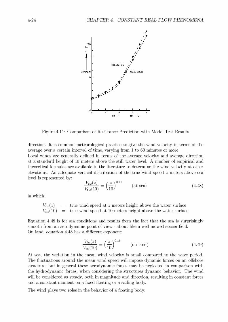
4-24 CHAPTER 4. CONSTANT REAL FLOW PHENOMENA
Figure 4.11: Comparison of Resistance Prediction with Model Test Results
direction. It is common meteorological practice to give the wind velocity in terms of theaverage over a certain interval of time, varying from 1 to 60 minutes or more.Local winds are generally de…ned in terms of the average velocity and average directionat a standard height of 10 meters above the still water level. A number of empirical andtheoretical formulas are available in the literature to determine the wind velocity at otherelevations. An adequate vertical distribution of the true wind speed z meters above sealevel is represented by:
Vtw(z)
Vtw(10)=
³ z10
´0:11(at sea) (4.48)
in which:
Vtw(z) = true wind speed at z meters height above the water surfaceVtw(10) = true wind speed at 10 meters height above the water surface
Equation 4.48 is for sea conditions and results from the fact that the sea is surprisinglysmooth from an aerodynamic point of view - about like a well mowed soccer …eld.On land, equation 4.48 has a di¤erent exponent:
Vtw(z)
Vtw(10)=
³ z10
´0:16(on land) (4.49)
At sea, the variation in the mean wind velocity is small compared to the wave period.The ‡uctuations around the mean wind speed will impose dynamic forces on an o¤shorestructure, but in general these aerodynamic forces may be neglected in comparison withthe hydrodynamic forces, when considering the structures dynamic behavior. The windwill be considered as steady, both in magnitude and direction, resulting in constant forcesand a constant moment on a …xed ‡oating or a sailing body.
The wind plays two roles in the behavior of a ‡oating body:
4.8. WIND LOADS 4-25
² Its …rst is a direct role, where the wind exerts a force on the part of the structureexposed to the air. Wind forces are exerted due to the ‡ow of air around the variousparts. Only local winds are needed for the determination of these forces.
² The second is an indirect role. Winds generate waves and currents and throughthese in‡uence a ship indirectly too. To determine these wind e¤ects, one needsinformation about the wind and storm conditions in a much larger area. Wave andcurrent generation is a topic for oceanographers; the e¤ects of waves and currents on‡oating bodies will be dealt with separately in later chapters.
Only the direct in‡uence of the winds will be discussed here.Forces and moments will be caused by the speed of the wind relative to the (moving) body.The forces and moments which the wind exerts on a structure can therefore be computedby:
¯¯Xw =
1
2½airV 2rw ¢ CXw(®rw) ¢ AT
¯¯
¯¯Yw =
1
2½airV 2rw ¢ CYw(®rw) ¢ AL
¯¯
¯¯Nw =
1
2½airV 2rw ¢ CNw(®rw) ¢ AL ¢ L
¯¯ (4.50)
in which:
Xw = steady longitudinal wind force (N)Yw = steady lateral wind force (N)Nw = steady horizontal wind moment (Nm)½air ¼ ½water=800 = density of air (kg/m3)Vrw = relative wind velocity (m/s)®rw = relative wind direction (-), from astern is zeroAT = transverse projected wind area (m2)AL = lateral projected wind area (m2)L = length of the ship (m)C¤w(®rw) = ®rw-dependent wind load coe¢cient (-)
Note that it is a ”normal” convention to refer to the true wind direction as the directionfrom which the wind comes, while waves and currents are usually referred to in terms ofwhere they are going. A North-West wind will cause South-East waves, therefore!
4.8.1 Wind Loads on Moored Ships
For moored ships, only the true wind speed and direction determine the longitudinal andlateral forces and the yaw moment on the ship, as given in …gure 4.12. Because of theabsence of a steady velocity of the structure, the relative wind is similar to the true wind:
jVrw = Vtwj and j®rw = ®twj (4.51)
The total force and moment experienced by an object exposed to the wind is partly ofviscous origin (pressure drag) and partly due to potential e¤ects (lift force). For blunt
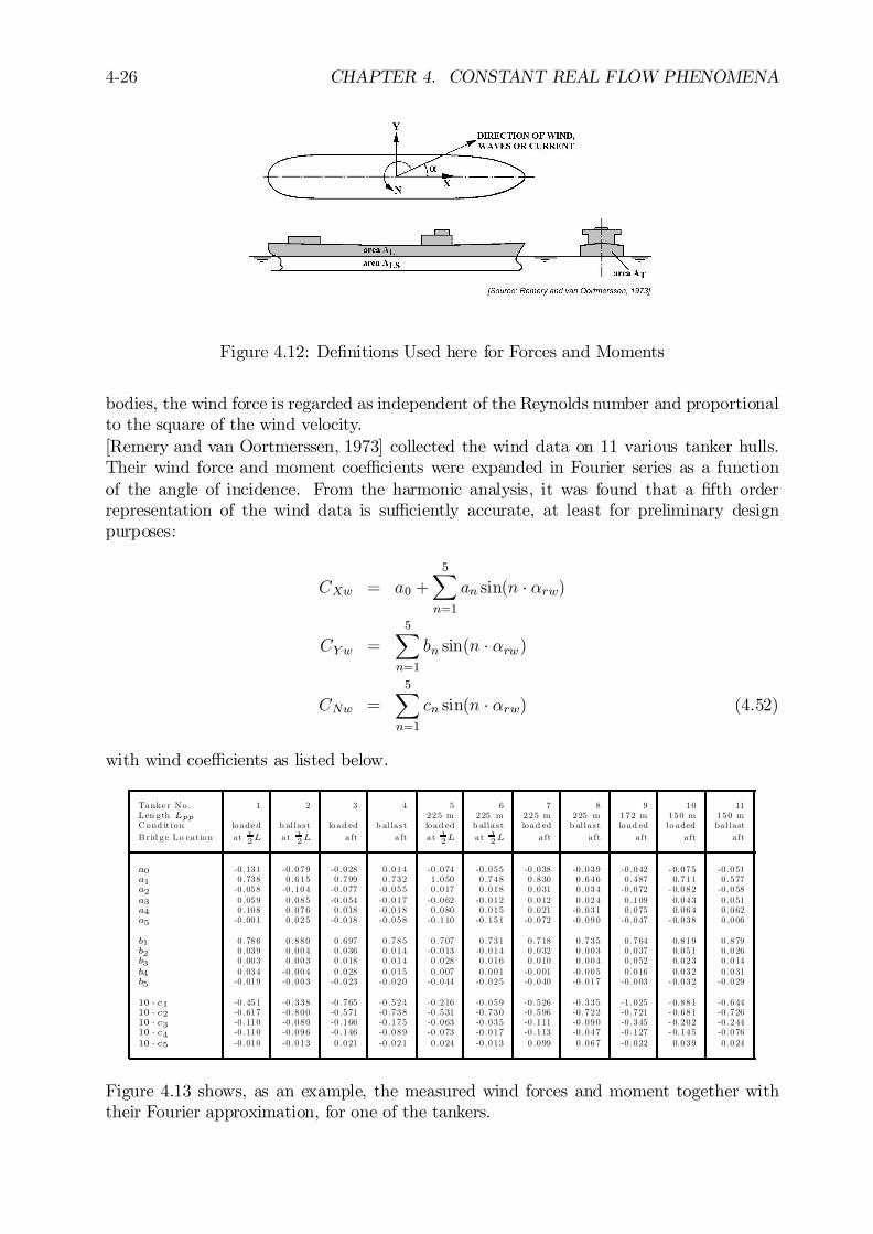
4-26 CHAPTER 4. CONSTANT REAL FLOW PHENOMENA
Figure 4.12: De…nitions Used here for Forces and Moments
bodies, the wind force is regarded as independent of the Reynolds number and proportionalto the square of the wind velocity.[Remery and van Oortmerssen, 1973] collected the wind data on 11 various tanker hulls.Their wind force and moment coe¢cients were expanded in Fourier series as a functionof the angle of incidence. From the harmonic analysis, it was found that a …fth orderrepresentation of the wind data is su¢ciently accurate, at least for preliminary designpurposes:
CXw = a0 +5X
n=1
an sin(n ¢ ®rw)
CYw =5X
n=1
bn sin(n ¢ ®rw)
CNw =5X
n=1
cn sin(n ¢ ®rw) (4.52)
with wind coe¢cients as listed below.
Tanke r No . 1 2 3 4 5 6 7 8 9 10 11Len gth Lpp 225 m 225 m 225 m 225 m 172 m 150 m 150 mCond it ion loade d b alla st load ed b alla st load ed b alla st load ed b alla st load ed loaded ba lla stB rid ge Lo cat ion at 1
2L at 12L a ft a ft a t 1
2L at 12L a ft a ft a ft a ft a ft
a0 -0 .131 -0 .079 -0 .028 0 .014 -0 .074 -0 .055 -0 .038 -0 .039 -0 .042 - 0.075 -0 .051a1 0 .738 0 .615 0 .799 0 .732 1 .050 0 .748 0 .830 0 .646 0 .487 0.711 0 .577a2 -0 .058 -0 .104 -0 .077 -0 .055 0 .017 0 .018 0 .031 0 .034 -0 .072 - 0.082 -0 .058a3 0 .059 0 .085 -0 .054 -0 .017 -0 .062 -0 .012 0 .012 0 .024 0 .109 0.043 0 .051a4 0 .108 0 .076 0 .018 -0 .018 0 .080 0 .015 0 .021 -0 .031 0 .075 0.064 0 .062a5 -0 .001 0 .025 -0 .018 -0 .058 -0 .110 -0 .151 -0 .072 -0 .090 -0 .047 - 0.038 0 .006
b1 0 .786 0 .880 0 .697 0 .785 0 .707 0 .731 0 .718 0 .735 0 .764 0.819 0 .879b2 0 .039 0 .004 0 .036 0 .014 -0 .013 -0 .014 0 .032 0 .003 0 .037 0.051 0 .026b3 0 .003 0 .003 0 .018 0 .014 0 .028 0 .016 0 .010 0 .004 0 .052 0.023 0 .014b4 0 .034 -0 .004 0 .028 0 .015 0 .007 0 .001 -0 .001 -0 .005 0 .016 0.032 0 .031b5 -0 .019 -0 .003 -0 .023 -0 .020 -0 .044 -0 .025 -0 .040 -0 .017 -0 .003 - 0.032 -0 .029
10 ¢ c1 -0 .451 -0 .338 -0 .765 -0 .524 -0 .216 -0 .059 -0 .526 -0 .335 -1 .025 - 0.881 -0 .64410 ¢ c2 -0 .617 -0 .800 -0 .571 -0 .738 -0 .531 -0 .730 -0 .596 -0 .722 -0 .721 - 0.681 -0 .72610 ¢ c3 -0 .110 -0 .080 -0 .166 -0 .175 -0 .063 -0 .035 -0 .111 -0 .090 -0 .345 - 0.202 -0 .24410 ¢ c4 -0 .110 -0 .096 -0 .146 -0 .089 -0 .073 -0 .017 -0 .113 -0 .047 -0 .127 - 0.145 -0 .07610 ¢ c5 -0 .010 -0 .013 0 .021 -0 .021 0 .024 -0 .013 0 .099 0 .067 -0 .022 0.039 0 .024
Figure 4.13 shows, as an example, the measured wind forces and moment together withtheir Fourier approximation, for one of the tankers.
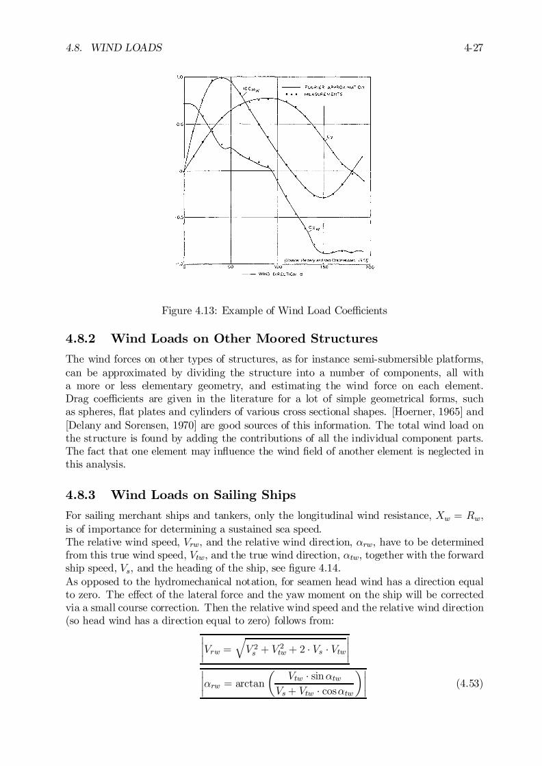
4.8. WIND LOADS 4-27
Figure 4.13: Example of Wind Load Coe¢cients
4.8.2 Wind Loads on Other Moored Structures
The wind forces on other types of structures, as for instance semi-submersible platforms,can be approximated by dividing the structure into a number of components, all witha more or less elementary geometry, and estimating the wind force on each element.Drag coe¢cients are given in the literature for a lot of simple geometrical forms, suchas spheres, ‡at plates and cylinders of various cross sectional shapes. [Hoerner, 1965] and[Delany and Sorensen, 1970] are good sources of this information. The total wind load onthe structure is found by adding the contributions of all the individual component parts.The fact that one element may in‡uence the wind …eld of another element is neglected inthis analysis.
4.8.3 Wind Loads on Sailing Ships
For sailing merchant ships and tankers, only the longitudinal wind resistance, Xw = Rw,is of importance for determining a sustained sea speed.The relative wind speed, Vrw, and the relative wind direction, ®rw, have to be determinedfrom this true wind speed, Vtw, and the true wind direction, ®tw, together with the forwardship speed, Vs, and the heading of the ship, see …gure 4.14.As opposed to the hydromechanical notation, for seamen head wind has a direction equalto zero. The e¤ect of the lateral force and the yaw moment on the ship will be correctedvia a small course correction. Then the relative wind speed and the relative wind direction(so head wind has a direction equal to zero) follows from:
¯¯Vrw =
qV 2s + V
2tw+ 2 ¢ Vs ¢ Vtw
¯¯
¯¯®rw = arctan
µVtw ¢ sin®tw
Vs+ Vtw ¢ cos®tw
¶¯¯ (4.53)
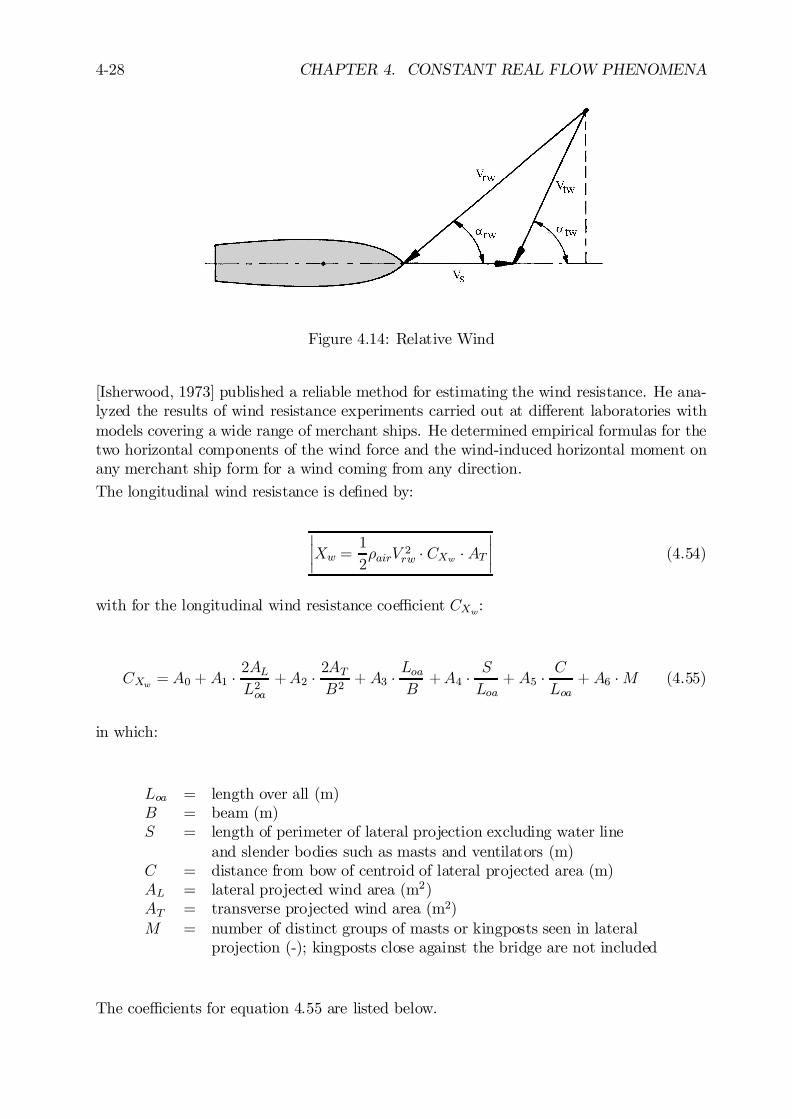
4-28 CHAPTER 4. CONSTANT REAL FLOW PHENOMENA
Figure 4.14: Relative Wind
[Isherwood, 1973] published a reliable method for estimating the wind resistance. He ana-lyzed the results of wind resistance experiments carried out at di¤erent laboratories withmodels covering a wide range of merchant ships. He determined empirical formulas for thetwo horizontal components of the wind force and the wind-induced horizontal moment onany merchant ship form for a wind coming from any direction.
The longitudinal wind resistance is de…ned by:
¯¯Xw =
1
2½airV 2rw ¢ CXw ¢ AT
¯¯ (4.54)
with for the longitudinal wind resistance coe¢cient CXw:
CXw = A0 + A1 ¢ 2ALL2oa
+A2 ¢ 2ATB2
+ A3 ¢ LoaB+A4 ¢ S
Loa+ A5 ¢ C
Loa+ A6 ¢M (4.55)
in which:
Loa = length over all (m)B = beam (m)S = length of perimeter of lateral projection excluding water line
and slender bodies such as masts and ventilators (m)C = distance from bow of centroid of lateral projected area (m)AL = lateral projected wind area (m2)AT = transverse projected wind area (m2)M = number of distinct groups of masts or kingposts seen in lateral
projection (-); kingposts close against the bridge are not included
The coe¢cients for equation 4.55 are listed below.
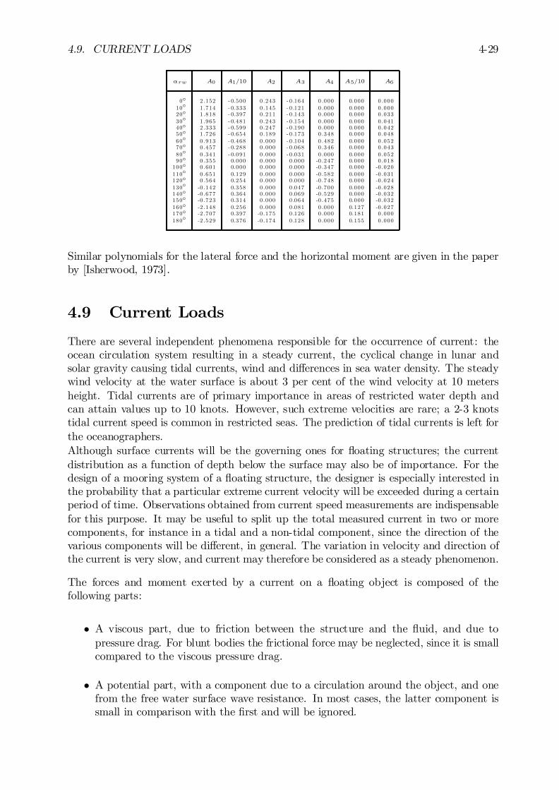
4.9. CURRENT LOADS 4-29
®rw A0 A1=10 A2 A3 A4 A5=10 A6
0± 2 .152 - 0.500 0 .243 - 0 .164 0 .000 0.000 0 .00010± 1 .714 - 0.333 0 .145 - 0 .121 0 .000 0.000 0 .00020± 1 .818 - 0.397 0 .211 - 0 .143 0 .000 0.000 0 .03330± 1 .965 - 0.481 0 .243 - 0 .154 0 .000 0.000 0 .04140± 2 .333 - 0.599 0 .247 - 0 .190 0 .000 0.000 0 .04250± 1 .726 - 0.654 0 .189 - 0 .173 0 .348 0.000 0 .04860± 0 .913 - 0.468 0 .000 - 0 .104 0 .482 0.000 0 .05270± 0 .457 - 0.288 0 .000 - 0 .068 0 .346 0.000 0 .04380± 0 .341 - 0.091 0 .000 - 0 .031 0 .000 0.000 0 .05290± 0 .355 0.000 0 .000 0 .000 -0 .247 0.000 0 .018
100± 0 .601 0.000 0 .000 0 .000 -0 .347 0.000 -0 .020110± 0 .651 0.129 0 .000 0 .000 -0 .582 0.000 -0 .031120± 0 .564 0.254 0 .000 0 .000 -0 .748 0.000 -0 .024130± -0 .142 0.358 0 .000 0 .047 -0 .700 0.000 -0 .028140± -0 .677 0.364 0 .000 0 .069 -0 .529 0.000 -0 .032150± -0 .723 0.314 0 .000 0 .064 -0 .475 0.000 -0 .032160± -2 .148 0.256 0 .000 0 .081 0 .000 0.127 -0 .027170± -2 .707 0.397 -0 .175 0 .126 0 .000 0.181 0 .000180± -2 .529 0.376 -0 .174 0 .128 0 .000 0.155 0 .000
Similar polynomials for the lateral force and the horizontal moment are given in the paperby [Isherwood, 1973].
4.9 Current Loads
There are several independent phenomena responsible for the occurrence of current: theocean circulation system resulting in a steady current, the cyclical change in lunar andsolar gravity causing tidal currents, wind and di¤erences in sea water density. The steadywind velocity at the water surface is about 3 per cent of the wind velocity at 10 metersheight. Tidal currents are of primary importance in areas of restricted water depth andcan attain values up to 10 knots. However, such extreme velocities are rare; a 2-3 knotstidal current speed is common in restricted seas. The prediction of tidal currents is left forthe oceanographers.Although surface currents will be the governing ones for ‡oating structures; the currentdistribution as a function of depth below the surface may also be of importance. For thedesign of a mooring system of a ‡oating structure, the designer is especially interested inthe probability that a particular extreme current velocity will be exceeded during a certainperiod of time. Observations obtained from current speed measurements are indispensablefor this purpose. It may be useful to split up the total measured current in two or morecomponents, for instance in a tidal and a non-tidal component, since the direction of thevarious components will be di¤erent, in general. The variation in velocity and direction ofthe current is very slow, and current may therefore be considered as a steady phenomenon.
The forces and moment exerted by a current on a ‡oating object is composed of thefollowing parts:
² A viscous part, due to friction between the structure and the ‡uid, and due topressure drag. For blunt bodies the frictional force may be neglected, since it is smallcompared to the viscous pressure drag.
² A potential part, with a component due to a circulation around the object, and onefrom the free water surface wave resistance. In most cases, the latter component issmall in comparison with the …rst and will be ignored.

4-30 CHAPTER 4. CONSTANT REAL FLOW PHENOMENA
The forces and moments, as given in …gure 4.12, exerted by the current on a ‡oatingstructure can be calculated from:
¯¯Xc =
1
2½ ¢ V 2c ¢ CXc(®c) ¢ ATS
¯¯
¯¯Yc =
1
2½ ¢ V 2c ¢ CY c(®c) ¢ ALS
¯¯
¯¯Nc =
1
2½ ¢ V 2c ¢ CNc(®c) ¢ ALS ¢ L
¯¯ (4.56)
in which:
Xc = steady longitudinal current force (N)Yc = steady lateral current force (N)Nc = steady yaw current moment (Nm)½ = density of water (kg/m3)Vc = current velocity (m/s)®c = current direction, from astern is zero (rad)ATS ¼ B ¢ T = submerged transverse projected area (m2)ALS ¼ L ¢ T = submerged lateral projected area (m2)L = length of the ship (m)B = breadth of the ship (m)T = draft of the ship (m)C¡c(®c) = ®c-depending current load coe¢cient (-)
Results of model tests are given in the literature for various types of structures and vessels.
4.9.1 Current Loads on Moored Tankers
[Remery and van Oortmerssen, 1973] published current loads on several tanker models ofdi¤erent sizes, tested at MARIN. The coe¢cients CXc, CY c and CNc were calculated fromthese results. A tanker hull is a rather slender body for a ‡ow in the longitudinal directionand consequently the longitudinal force is mainly frictional. The total longitudinal forcewas very small for relatively low current speeds and could not be measured accurately.Moreover, extrapolation to full scale dimensions is di¢cult, since the longitudinal force isa¤ected by scale e¤ects.For mooring problems the longitudinal force will hardly be of importance. An estimate ofits magnitude can be made by calculating the ‡at plate frictional resistance, according tothe ITTC skin friction line as given in equation 4.42:
¯¯Xc =
0:075
(log10 (Rn) ¡ 2)2 ¢ 12½Vc
2 ¢ cos®c ¢ j cos®cj ¢ S¯¯ (4.57)
while:
Rn =Vc ¢ j cos®cj ¢ L
º(4.58)
with:
4.9. CURRENT LOADS 4-31
S ¼ L ¢ (B + 2T) = wetted surface of the ship (m2)L = length of the ship (m)B = breadth of the ship (m)T = draft of the ship (m)Vc = current velocity (m/s)®c = current direction (-), from astern is zero½ = density of water (ton/m3)Rn = Reynolds number (-)º = kinematic viscosity of water (m2s)
Extrapolation of the transverse force and yaw moment to prototype values is no problem.For ‡ow in the transverse direction a tanker is a blunt body and, since the bilge radius issmall, ‡ow separation occurs in the model in the same way as in the prototype. Therefore,the transverse force coe¢cient and the yaw moment coe¢cient are independent of theReynolds number.The coe¢cients for the transverse force and the yaw moment were expanded by MARINin a Fourier series, as was done for the wind load coe¢cients as described in a previoussection:
CY c(®c) =5X
n=1
bn ¢ sin(n ¢ ®c)
CNc(®c) =5X
n=1
cn ¢ sin(n ¢ ®c) (4.59)
The average values of the coe¢cients bn and cn for the …fth order Fourier series, as publishedby [Remery and van Oortmerssen, 1973], are given in the table below.
n bn 10 ¢ cn
1 0 .908 -0 .2522 0 .000 -0 .9043 -0 .116 0 .0324 0 .000 0 .1095 -0 .033 0 .011
These results are valid for deep water. For shallow water, the transverse current force andmoment coe¢cients have to be multiplied by a coe¢cient, which is given in …gure 4.15.The in‡uence of the free surface is included in the data given on the coe¢cients bn andcn in the previous table. This in‡uence, however, depends on the water depth and on theFroude number, and consequently changes if the current velocity or the tanker dimensionschange. For the condition to which these data apply, deep water and a prototype currentspeed in the order of 3 knots, the e¤ect of the free surface is very small. For the case of asmall clearance under the keel and a current direction of 90 degrees, damming up of thewater at the weather side and a lowering of the water at the lee side of the ship occurs.
4.9.2 Current Loads on Other Moored Structures
Current loads on other types of ‡oating structures are usually estimated in the same wayas is used for wind loads.
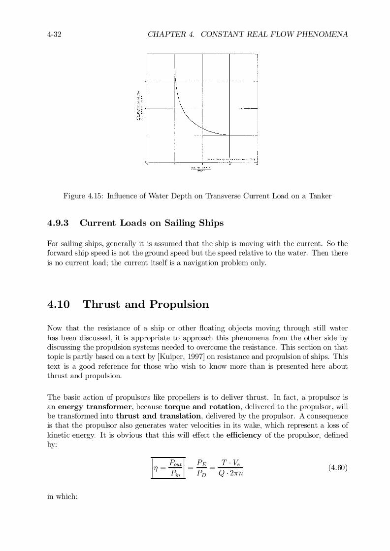
4-32 CHAPTER 4. CONSTANT REAL FLOW PHENOMENA
Figure 4.15: In‡uence of Water Depth on Transverse Current Load on a Tanker
4.9.3 Current Loads on Sailing Ships
For sailing ships, generally it is assumed that the ship is moving with the current. So theforward ship speed is not the ground speed but the speed relative to the water. Then thereis no current load; the current itself is a navigation problem only.
4.10 Thrust and Propulsion
Now that the resistance of a ship or other ‡oating objects moving through still waterhas been discussed, it is appropriate to approach this phenomena from the other side bydiscussing the propulsion systems needed to overcome the resistance. This section on thattopic is partly based on a text by [Kuiper, 1997] on resistance and propulsion of ships. Thistext is a good reference for those who wish to know more than is presented here aboutthrust and propulsion.
The basic action of propulsors like propellers is to deliver thrust. In fact, a propulsor isan energy transformer, because torque and rotation, delivered to the propulsor, willbe transformed into thrust and translation, delivered by the propulsor. A consequenceis that the propulsor also generates water velocities in its wake, which represent a loss ofkinetic energy. It is obvious that this will e¤ect the e¢ciency of the propulsor, de…nedby:
¯¯´ = Pout
Pin
¯¯ = PE
PD=
T ¢ VeQ ¢ 2¼n (4.60)
in which:
4.10. THRUST AND PROPULSION 4-33
´ = propulsive e¢ciency (-)PD = delivered power, delivered to the propulsor (Nm/s = W)PE = e¤ective power, delivered by the propulsor (Nm/s = W)Q = torque delivered to the propulsor (Nm)n = number of revolutions (1/s)T = thrust delivered by the propulsor (N)Ve = mean entrance speed of water in propeller disk,
also called advance velocity with notation Va (m/s)
The e¢ciency varies widely between various types of propulsors, but the screw propellerhas not yet been equalled in most cases and is therefore the most commonly used propulsor.The propulsor is generally mounted behind the hull. This is because of e¢ciency; the waterwhich is brought into motion by the friction along the ship is reversed by the propelleraction and as a result less energy is left behind in the water.A risk for every propulsor operating at high rotational velocities is cavitation. This occurswhen the local pressure, associated with high local velocities in the ‡uid, is lower than thevapor pressure. As a result the water starts to boil locally and water-vapour …lled cavitiesare formed. When these vapor-…lled (not air-…lled) cavities in the wake arrive in regionswith a higher pressure they collapse violently, causing local shock waves in the water thatcan erode the nearby surface. This dynamic behavior of large cavities can also generatevibrations in the ship structure.
4.10.1 Propulsors
The most important propulsors used for shipping and o¤shore activities include:
² Fixed Pitch Propellers, see …gure 4.16-a.The most common propulsor is the …xed pitch open screw propeller (FPP) which,as all propellers, generates a propulsive force by lift on the propeller blades. Theseblade sections are similar to those of airfoils, operating at some angle of attack inthe ‡ow. The geometry of the propeller blades is quite critical with respect to theoccurrence of cavitation. Therefore, a speci…c propeller is generally designed for thespeci…c circumstances of each ship and its engine. The thrust, and consequentlythe speed of the ship, is controlled by the propeller rotational speed - often calledrevolutions or rpm (for revolutions per minute).
² Controllable Pitch Propellers, see …gure 4.16-b.In the case of a controllable pitch propeller (CPP) the thrust is controlled by changingthe pitch of the blades. The shaft often has a constant rotational speed. A CCP isoften used when the propeller has to operate at more than one design condition - suchas free running and towing for a tug. It is also e¤ective when rapid manoeuveringis required or when shaft generators, which require a constant rpm, are present.Reversing the thrust occurs by changing the pitch with constant revolutions in thesame direction. This signi…cantly decreases the time required to change the directionof the thrust. It is important to keep in mind that the CPP has only one designpitch; changing the pitch always reduces the e¢ciency.
² Ducted Propellers, see …gure 4.16-c.At high propeller loadings a duct increases the propeller e¢ciency. A duct generates

4-34 CHAPTER 4. CONSTANT REAL FLOW PHENOMENA
Figure 4.16: Di¤erent Propulsion Con…gurations
part of the total thrust due to its interaction with the propeller. This is the case withan accelerating duct, in which the ‡ow velocity is increased due to the duct. Ductedpropellers are used in a wide range of applications with heavily loaded propellers,such as for tugs. Several types of ducts, sometimes asymmetric and sometimes atsome distance upstream of the propeller, have been designed to make the propellerin‡ow more uniform.
² Thrusters, see …gures 4.16-d and 4.16-e.A propeller can be driven from above by a vertical shaft. This makes it possibleto rotate the propeller along the vertical axis and to generate thrust in any chosendirection. These con…gurations are called thrusters. They can have an open propeller,but very often a duct is also used. The right angle drive of a thruster makes itmore complicated and thus more expensive and vulnerable than a normal propellershaft. Also the hub diameter is larger, which slightly decreases e¢ciency. There aresome interesting advantages however. The propeller can be in front of the vertical
4.10. THRUST AND PROPULSION 4-35
shaft (towing) as well as behind it (pushing). In the towing mode the in‡ow ismore uniform; this decreases vibrations and cavitation. A steerable or azimuthingthruster may rotate around a vertical axis which makes it possible to steer with it.This makes it easier to manoeuver, especially at low speeds. They are common fordynamic positioning; the steerable direction of its thrust is fully utilized in that case.
² Cycloidal or Voiht-Schneider Propellers, see …gures 4.16-f and 4.16-h.A very special propulsor is the cycloidal propeller, also called Voiht-Schneider pro-peller after its main developer. It consists of a number of foils on a rotating plate.These foils can rotate relative to this plate and their position is such that they arealways perpendicular to the radii from a moving center point, P , as shown in …gure4.16-h. When this center point is in the center of the blade circle, there is no resultingforce. When this center point is moved, a thrust is generated perpendicular to thedirection in which the center point is shifted. Thus thrust can be applied in anydirection just by moving the center point; rudders can be omitted. This propulsivesystem can be used for tugs and supply boats, for which maneuvering is important.Its e¢ciency, however, is lower than that of an open propeller due to the fact that theblades generate thrust over a part of their revolution only, while viscous resistanceis present over the whole revolution. Voith-Schneider propellers must be mountedunder a ‡at bottom; a bottom cover is sometimes provided for protection (see …gure4.16-f).
² Water Jets, see …gure 4.16-g.This propulsor accelerates water using a pump inside the hull, instead of a propelleroutside the hull. The water is drawn in from the bottom of the ship, is acceleratedinside the ship by a pump and leaves the ship at the stern. This has many advantageswhen a propeller is too vulnerable to damage, or when a propeller is too dangerousas is the case for rescue vessels. Rudders can be omitted because of the rotatingpossibilities of the outlet and excellent manoeuvering qualities can be obtained, asfor instance are required for pilot vessels. A pump jet can be useful in shallow water.However, the inner surface of the pump system is large and the velocities inside arehigh; the viscous losses are high, too. The e¢ciency is therefore lower than that ofan open propeller.
4.10.2 Propeller Geometry
First some general geometrical de…nitions of the propeller are given. A sketch of a righthanded propeller is given in …gure 4.17-a.
² The propeller blades are attached to the hub, which is attached to the end ofthe propeller shaft. The propeller rotates about the shaft center line. The directionof rotation is as viewed from behind, that is towards the shaft. In normal forwardoperation a right handed propeller rotates in clockwise direction when viewedfrom behind.The propeller hub is, of course, rotational symmetric because it should not disturbthe ‡ow. The attachment of the propeller blade to the hub is a gradual transition,which is done in the …llet area or the blade root. A streamlined cap is generally…tted to the hub at the end of its shaft.
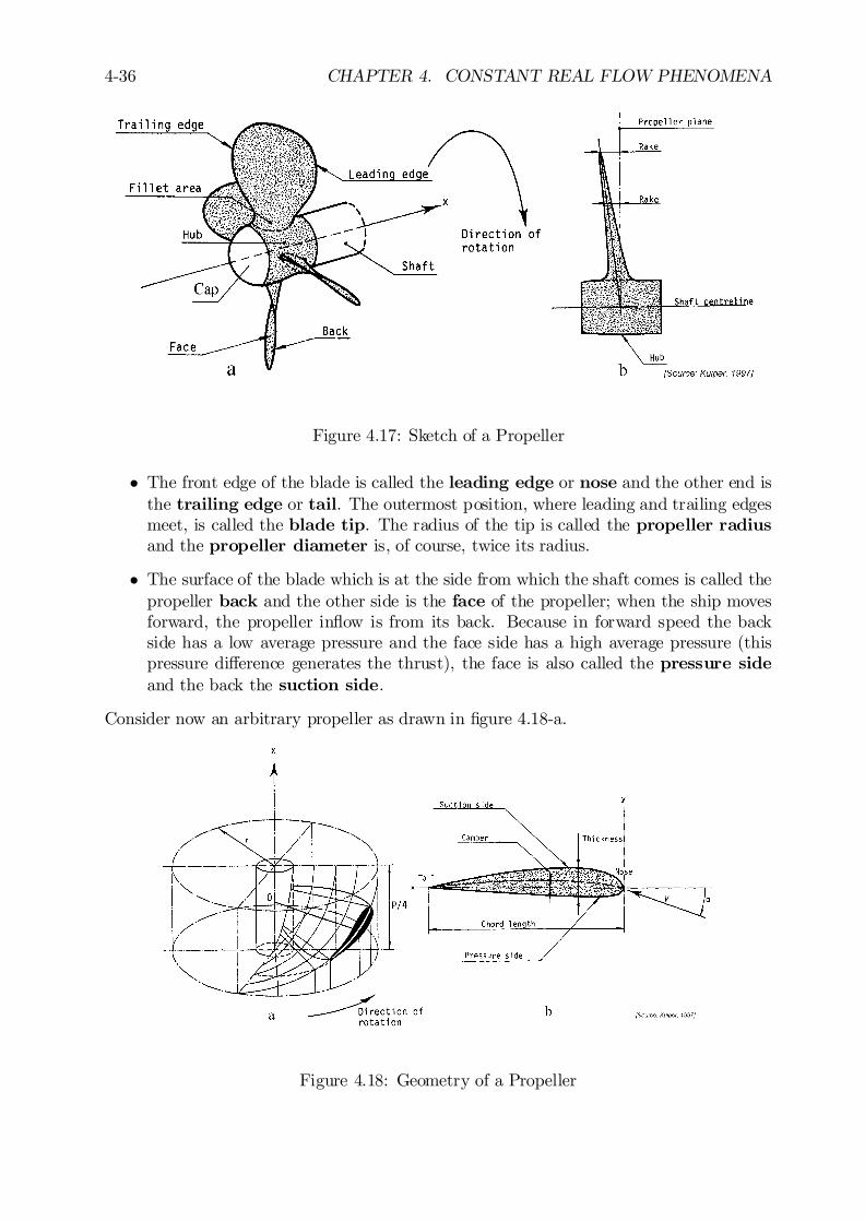
4-36 CHAPTER 4. CONSTANT REAL FLOW PHENOMENA
Figure 4.17: Sketch of a Propeller
² The front edge of the blade is called the leading edge or nose and the other end isthe trailing edge or tail. The outermost position, where leading and trailing edgesmeet, is called the blade tip. The radius of the tip is called the propeller radiusand the propeller diameter is, of course, twice its radius.
² The surface of the blade which is at the side from which the shaft comes is called thepropeller back and the other side is the face of the propeller; when the ship movesforward, the propeller in‡ow is from its back. Because in forward speed the backside has a low average pressure and the face side has a high average pressure (thispressure di¤erence generates the thrust), the face is also called the pressure sideand the back the suction side.
Consider now an arbitrary propeller as drawn in …gure 4.18-a.
Figure 4.18: Geometry of a Propeller
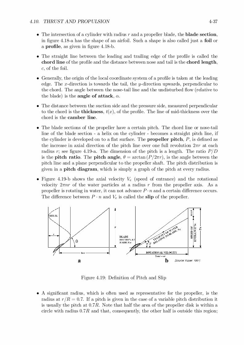
4.10. THRUST AND PROPULSION 4-37
² The intersection of a cylinder with radius r and a propeller blade, the blade section,in …gure 4.18-a has the shape of an airfoil. Such a shape is also called just a foil ora pro…le, as given in …gure 4.18-b.
² The straight line between the leading and trailing edge of the pro…le is called thechord line of the pro…le and the distance between nose and tail is the chord length,c, of the foil.
² Generally, the origin of the local coordinate system of a pro…le is taken at the leadingedge. The x-direction is towards the tail, the y-direction upwards, perpendicular tothe chord. The angle between the nose-tail line and the undisturbed ‡ow (relative tothe blade) is the angle of attack, ®.
² The distance between the suction side and the pressure side, measured perpendicularto the chord is the thickness, t(x), of the pro…le. The line of mid-thickness over thechord is the camber line.
² The blade sections of the propeller have a certain pitch. The chord line or nose-tailline of the blade section - a helix on the cylinder - becomes a straight pitch line, ifthe cylinder is developed on to a ‡at surface. The propeller pitch, P , is de…ned asthe increase in axial direction of the pitch line over one full revolution 2¼r at eachradius r; see …gure 4.19-a. The dimension of the pitch is a length. The ratio P=Dis the pitch ratio. The pitch angle, µ = arctan (P=2¼r), is the angle between thepitch line and a plane perpendicular to the propeller shaft. The pitch distribution isgiven in a pitch diagram, which is simply a graph of the pitch at every radius.
² Figure 4.19-b shows the axial velocity Ve (speed of entrance) and the rotationalvelocity 2¼nr of the water particles at a radius r from the propeller axis. As apropeller is rotating in water, it can not advance P ¢n and a certain di¤erence occurs.The di¤erence between P ¢ n and Ve is called the slip of the propeller.
Figure 4.19: De…nition of Pitch and Slip
² A signi…cant radius, which is often used as representative for the propeller, is theradius at r=R = 0:7. If a pitch is given in the case of a variable pitch distribution itis usually the pitch at 0:7R. Note that half the area of the propeller disk is within acircle with radius 0:7R and that, consequently, the other half is outside this region;
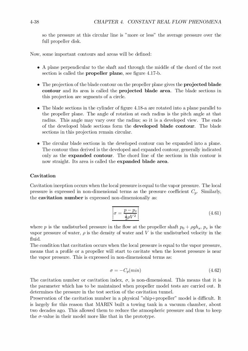
4-38 CHAPTER 4. CONSTANT REAL FLOW PHENOMENA
so the pressure at this circular line is ”more or less” the average pressure over thefull propeller disk.
Now, some important contours and areas will be de…ned:
² A plane perpendicular to the shaft and through the middle of the chord of the rootsection is called the propeller plane, see …gure 4.17-b.
² The projection of the blade contour on the propeller plane gives the projected bladecontour and its area is called the projected blade area. The blade sections inthis projection are segments of a circle.
² The blade sections in the cylinder of …gure 4.18-a are rotated into a plane parallel tothe propeller plane. The angle of rotation at each radius is the pitch angle at thatradius. This angle may vary over the radius; so it is a developed view. The endsof the developed blade sections form the developed blade contour. The bladesections in this projection remain circular.
² The circular blade sections in the developed contour can be expanded into a plane.The contour thus derived is the developed and expanded contour, generally indicatedonly as the expanded contour. The chord line of the sections in this contour isnow straight. Its area is called the expanded blade area.
Cavitation
Cavitation inception occurs when the local pressure is equal to the vapor pressure. The localpressure is expressed in non-dimensional terms as the pressure coe¢cient Cp. Similarly,the cavitation number is expressed non-dimensionally as:
¯¯¾ = p¡ pv
12½V
2
¯¯ (4.61)
where p is the undisturbed pressure in the ‡ow at the propeller shaft p0 + ½ghs, pv is thevapor pressure of water, ½ is the density of water and V is the undisturbed velocity in the‡uid.The condition that cavitation occurs when the local pressure is equal to the vapor pressure,means that a pro…le or a propeller will start to cavitate when the lowest pressure is nearthe vapor pressure. This is expressed in non-dimensional terms as:
¾ = ¡Cp(min) (4.62)
The cavitation number or cavitation index, ¾, is non-dimensional. This means that it isthe parameter which has to be maintained when propeller model tests are carried out. Itdetermines the pressure in the test section of the cavitation tunnel.Preservation of the cavitation number in a physical ”ship+propeller” model is di¢cult. Itis largely for this reason that MARIN built a towing tank in a vacuum chamber, abouttwo decades ago. This allowed them to reduce the atmospheric pressure and thus to keepthe ¾-value in their model more like that in the prototype.
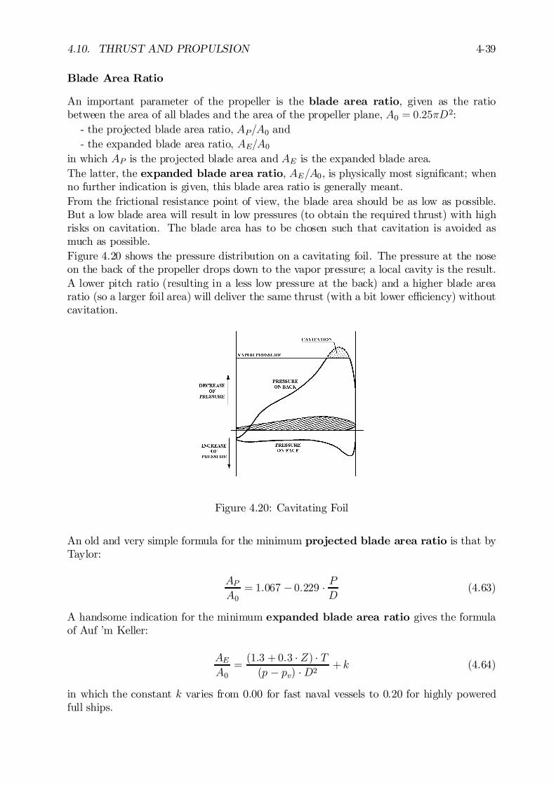
4.10. THRUST AND PROPULSION 4-39
Blade Area Ratio
An important parameter of the propeller is the blade area ratio, given as the ratiobetween the area of all blades and the area of the propeller plane, A0 = 0:25¼D2:
- the projected blade area ratio, AP=A0 and- the expanded blade area ratio, AE=A0
in which AP is the projected blade area and AE is the expanded blade area.The latter, the expanded blade area ratio, AE=A0, is physically most signi…cant; whenno further indication is given, this blade area ratio is generally meant.From the frictional resistance point of view, the blade area should be as low as possible.But a low blade area will result in low pressures (to obtain the required thrust) with highrisks on cavitation. The blade area has to be chosen such that cavitation is avoided asmuch as possible.Figure 4.20 shows the pressure distribution on a cavitating foil. The pressure at the noseon the back of the propeller drops down to the vapor pressure; a local cavity is the result.A lower pitch ratio (resulting in a less low pressure at the back) and a higher blade arearatio (so a larger foil area) will deliver the same thrust (with a bit lower e¢ciency) withoutcavitation.
Figure 4.20: Cavitating Foil
An old and very simple formula for the minimum projected blade area ratio is that byTaylor:
APA0
= 1:067 ¡ 0:229 ¢ PD
(4.63)
A handsome indication for the minimum expanded blade area ratio gives the formulaof Auf ’m Keller:
AEA0
=(1:3 + 0:3 ¢ Z) ¢ T(p ¡ pv) ¢D2 + k (4.64)
in which the constant k varies from 0.00 for fast naval vessels to 0.20 for highly poweredfull ships.

4-40 CHAPTER 4. CONSTANT REAL FLOW PHENOMENA
Number of Propeller Blades
The number of propeller blades, Z, is chosen in relation to possible vibrations. An 8cylinder engine and a 4 bladed propeller may su¤er from resonance frequencies becausethe blade passage frequency (the frequency at which a blade passes close to the rudder forexample) and the engine frequencies have common harmonics. In that case vibrations canbecome extensive, resulting in damage.The structure of the wake is also important for the choice of the number of blades. Whenthe wake has strong harmonics equal to the number of blades, thrust variations may becomelarge; these, too, can lead to vibrations.
Wageningen Propeller Series
Systematic series of propeller models have been tested by MARIN to form a basis forpropeller design. The starting point of a series is its parent form. The extent and applica-bility of the series depends on the parameters which are varied and on the range of theirvariations. Several series are described in the literature.The most extensive and widely used …xed pitch open propeller series is the WageningenB-series. The basic form of the B-series is simple and it has a good performance. Theextent of the series is large; some 210 propellers have been tested.
The following parameters of the B-series propellers have been varied:- the expanded blade area ratio, AE=A0, from 0.3 to 1.2- the number of blades, Z, from 2 to 7- the pitch ratio, P=D, from 0.5 to 1.4
The propellers are indicated by their number of blades and expanded blade area ratio. Forinstance, propeller B-4.85 has four blades and an expanded blade area ratio of 0.85. Thetest results are given in so-called open water diagrams per series of one blade number, onearea ratio and a range of pitch ratios. The open water tests of the B-series were done atvarious rotation rates, n, so at various Reynolds numbers. These results were corrected toa standard Reynolds number of Rn = 2 ¢ 106 along the lines of the ITTC method, as givenby equation 4.42. However, these corrections are very small.In addition to open …xed pitch propellers, MARIN has also developed series of …xed pitchpropellers in an accelerating nozzle (Ka-series) and series of controllable pitch propellers ina nozzle. All available information on MARIN systematic propeller series has been summa-rized by [Kuiper, 1992]. The propulsive characteristics have been described by polynomialsto make them usable in computer programs. Some other research institutes have also madetheir own propeller series, but the Wageningen Propeller Series are the most well known.
4.10.3 Propeller Mechanics
This section discusses the mechanics of a propeller in a uniform ‡ow - the so-called freerunning or open water condition.
Open Water Characteristics
Suppose an open water propeller translating with a constant forward speed, Ve, anda constant number of revolutions per second, n, is immersed in a homogeneous initiallystationary ‡uid without any currents or waves. Then, two velocity components can be
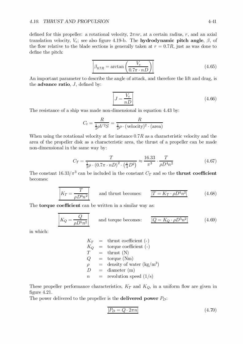
4.10. THRUST AND PROPULSION 4-41
de…ned for this propeller: a rotational velocity, 2¼nr, at a certain radius, r, and an axialtranslation velocity, Ve; see also …gure 4.19-b. The hydrodynamic pitch angle, ¯, ofthe ‡ow relative to the blade sections is generally taken at r = 0:7R, just as was done tode…ne the pitch:
¯¯¯0:7R = arctan
µVe
0:7¼ ¢ nD
¶¯¯ (4.65)
An important parameter to describe the angle of attack, and therefore the lift and drag, isthe advance ratio, J , de…ned by:
¯¯J = Ve
nD
¯¯ (4.66)
The resistance of a ship was made non-dimensional in equation 4.43 by:
Ct =R
12½V
2S=
R12½ ¢ (velocity)2 ¢ (area)
When using the rotational velocity at for instance 0:7R as a characteristic velocity and thearea of the propeller disk as a characteristic area, the thrust of a propeller can be madenon-dimensional in the same way by:
CT =T
12½ ¢ (0:7¼ ¢ nD)2 ¢
¡¼4D
2¢ ¼ 16:33
¼3¢ T
½D4n2(4.67)
The constant 16:33=¼3 can be included in the constant CT and so the thrust coe¢cientbecomes:
¯¯KT =
T
½D4n2
¯¯ and thrust becomes: jT =KT ¢ ½D4n2j (4.68)
The torque coe¢cient can be written in a similar way as:
¯¯KQ =
Q
½D5n2
¯¯ and torque becomes: jQ= KQ ¢ ½D5n2j (4.69)
in which:
KT = thrust coe¢cient (-)KQ = torque coe¢cient (-)T = thrust (N)Q = torque (Nm)½ = density of water (kg/m3)D = diameter (m)n = revolution speed (1/s)
These propeller performance characteristics, KT and KQ, in a uniform ‡ow are given in…gure 4.21.The power delivered to the propeller is the delivered power PD :
jPD = Q ¢ 2¼nj (4.70)
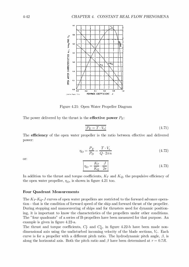
4-42 CHAPTER 4. CONSTANT REAL FLOW PHENOMENA
Figure 4.21: Open Water Propeller Diagram
The power delivered by the thrust is the e¤ective power PE :
jPE = T ¢ Vej (4.71)
The e¢ciency of the open water propeller is the ratio between e¤ective and deliveredpower:
´O =PEPD
=T ¢ VeQ ¢ 2¼n (4.72)
or: ¯¯´O =
KTKQ
¢ J2¼
¯¯ (4.73)
In addition to the thrust and torque coe¢cients, KT and KQ, the propulsive e¢ciency ofthe open water propeller, ´O, is shown in …gure 4.21 too.
Four Quadrant Measurements
TheKT-KQ-J curves of open water propellers are restricted to the forward advance opera-tion - that is the condition of forward speed of the ship and forward thrust of the propeller.During stopping and manoeuvering of ships and for thrusters used for dynamic position-ing, it is important to know the characteristics of the propellers under other conditions.The ”four quadrants” of a series of B-propellers have been measured for that purpose. Anexample is given in …gure 4.22-a.The thrust and torque coe¢cients, C¤T and C¤Q, in …gure 4.22-b have been made non-dimensional axis using the undisturbed incoming velocity of the blade sections, Vr. Eachcurve is for a propeller with a di¤erent pitch ratio. The hydrodynamic pitch angle, ¯, isalong the horizontal axis. Both the pitch ratio and ¯ have been determined at r = 0:7R.
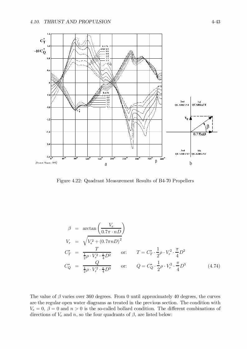
4.10. THRUST AND PROPULSION 4-43
Figure 4.22: Quadrant Measurement Results of B4-70 Propellers
¯ = arctan
µVe
0:7¼ ¢nD
¶
Vr =qV 2e + (0:7¼nD)
2
C¤T =T
12½ ¢ V 2r ¢ ¼
4D2
or: T = C¤T ¢ 12½ ¢ V 2r ¢ ¼
4D2
C¤Q =Q
12½ ¢ V 2r ¢ ¼4D3
or: Q= C¤Q ¢ 12½ ¢ V 2r ¢ ¼
4D3 (4.74)
The value of ¯ varies over 360 degrees. From 0 until approximately 40 degrees, the curvesare the regular open water diagrams as treated in the previous section. The condition withVe = 0, ¯ = 0 and n > 0 is the so-called bollard condition. The di¤erent combinations ofdirections of Ve and n, so the four quadrants of ¯, are listed below:
4-44 CHAPTER 4. CONSTANT REAL FLOW PHENOMENA
¯ Ve n
0±-90± Ve > 0 n > 090±-180± Ve > 0 n < 0180±-270± Ve < 0 n < 0270±-360± Ve < 0 n > 0
4.10.4 Ship Propulsion
This section treats the behavior of the propeller behind the ship and its interactionwith the ship.
Wake Fraction
The velocity de…cit behind the ship is a measure of its still water resistance. The velocityde…cit in the propeller plane (without the propeller present) can be integrated and averagedover the propeller plane. This velocity is the average entrance velocity, Ve, in the propellerplane when the propeller is absent. It is de…ned in terms of the ship speed, Vs, by thenominal wake fraction, wn:
wn =Vs ¡ VeVs
(4.75)
This de…nition is a non-dimensional form of the velocity de…cit, Vs ¡ Ve, in the propellerplane.The wake distribution is responsible for unsteadiness in the propeller loading during onerevolution, as can be seen in …gure 4.23. This …gure shows the lines with a constant wakefraction - thus lines with constant axial velocities of the ‡uid particles - at the propellerdisc behind various stern types of ships.Unsteady e¤ects will be neglected now and the (average) nominal wake fraction will be usedto obtain the (constant) open water propeller in‡ow, which yields the entrance velocity:
jVe = Vs ¢ (1¡ w)j with: w = wn (4.76)
For a statistical prediction of the wake fraction of ships, reference is given to regressionformulas of [Holtrop, 1984].
Thrust Deduction Fraction
The propeller has an e¤ect on the ship’s resistance, however. It increases the resistance ofthe ship by increasing the velocity along the hull (generally a small e¤ect) and by decreasingthe pressure around the stern. The thrust to be developed by the propeller should thus begreater than the resistance without propeller at the design speed, because the thrust hasto be equal to the increased resistance.The increase of resistance due to the propeller action is expressed as the thrust deductionfraction, t:
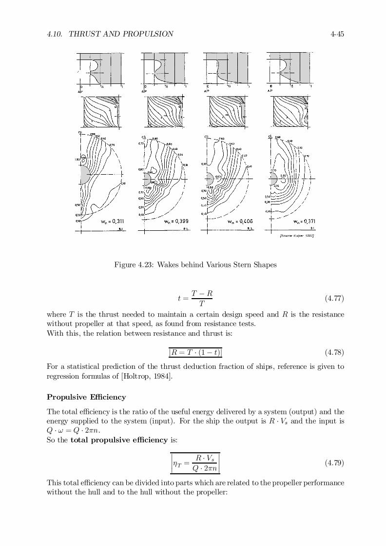
4.10. THRUST AND PROPULSION 4-45
Figure 4.23: Wakes behind Various Stern Shapes
t =T ¡RT
(4.77)
where T is the thrust needed to maintain a certain design speed and R is the resistancewithout propeller at that speed, as found from resistance tests.With this, the relation between resistance and thrust is:
jR = T ¢ (1¡ t)j (4.78)
For a statistical prediction of the thrust deduction fraction of ships, reference is given toregression formulas of [Holtrop, 1984].
Propulsive E¢ciency
The total e¢ciency is the ratio of the useful energy delivered by a system (output) and theenergy supplied to the system (input). For the ship the output is R ¢ Vs and the input isQ ¢ ! = Q ¢ 2¼n.So the total propulsive e¢ciency is:
¯¯´T =
R ¢ VsQ ¢ 2¼n
¯¯ (4.79)
This total e¢ciency can be divided into parts which are related to the propeller performancewithout the hull and to the hull without the propeller:
4-46 CHAPTER 4. CONSTANT REAL FLOW PHENOMENA
´T =R ¢ VsQ ¢ 2¼n
=T (1 ¡ t) ¢ Ve
1¡wQQO
¢QO ¢ 2¼n
=
µT ¢ VeQO ¢ 2¼n
¶¢µ1 ¡ t1 ¡ w
¶¢µQOQ
¶
=
µKTKQ
¢ J2¼
¶¢µ1¡ t1¡ w
¶¢µQOQ
¶(4.80)
or:j´T = ´O ¢ ´H ¢ ´Rj
in which, at the same thrust, QO is the torque of the open water propeller in a uniform‡ow and Q is the torque of the propeller in the wake behind the ship.
The total propulsive e¢ciency is thus divided into three components:
² Open Water E¢ciency:¯¯´O =
T ¢ VeQO ¢ 2¼n =
KTKQ
¢ J2¼
¯¯ (4.81)
This is the e¢ciency of the propeller alone in the mean (homogeneous) in‡ow, Ve. Itcan be derived from open water diagrams of propellers.
² Hull E¢ciency: ¯¯´H =
R ¢ VsT ¢ Ve
=1¡ t1¡ w
¯¯ (4.82)
Old but convenient rough approximations of the wake fraction and the thrust deduc-tion fraction of full scale ships are given by:
w ¼ 0:5 ¢ CB ¡ 0:05t ¼ 0:6 ¢ w (4.83)
where CB is the block coe¢cient of the ship. A fast slender container vessel withCB = 0:55will have ´H ¼ 1:12while for a crude oil carrier withCB = 0:85, ´H ¼ 1:24.So the e¤ect of a hull with its wake before the propeller increases the propulsivee¢ciency considerably. The propeller diameter therefore has to be such that thewake is going through the propeller disk as much as possible.When using model data, it should be noted that - contrarily to the thrust deductionfraction - the wake fraction is very sensitive for scale e¤ect. It is left to the reader toexplain this.
² Relative Rotative E¢ciency:¯¯´R =
QOQ
¯¯ (4.84)
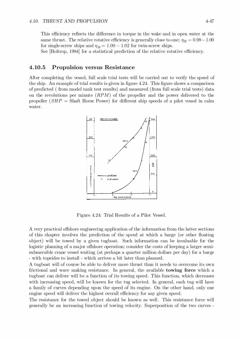
4.10. THRUST AND PROPULSION 4-47
This e¢ciency re‡ects the di¤erence in torque in the wake and in open water at thesame thrust. The relative rotative e¢ciency is generally close to one; ´R = 0:98¡1:00for single-screw ships and ´R = 1:00¡ 1:02 for twin-screw ships.See [Holtrop, 1984] for a statistical prediction of the relative rotative e¢ciency.
4.10.5 Propulsion versus Resistance
After completing the vessel, full scale trial tests will be carried out to verify the speed ofthe ship. An example of trial results is given in …gure 4.24. This …gure shows a comparisonof predicted ( from model tank test results) and measured (from full scale trial tests) dataon the revolutions per minute (RPM) of the propeller and the power delivered to thepropeller (SHP = Shaft Horse Power) for di¤erent ship speeds of a pilot vessel in calmwater.
Figure 4.24: Trial Results of a Pilot Vessel.
A very practical o¤shore engineering application of the information from the latter sectionsof this chapter involves the prediction of the speed at which a barge (or other ‡oatingobject) will be towed by a given tugboat. Such information can be invaluable for thelogistic planning of a major o¤shore operation; consider the costs of keeping a larger semi-submersible crane vessel waiting (at perhaps a quarter million dollars per day) for a barge- with topsides to install - which arrives a bit later than planned.A tugboat will of course be able to deliver more thrust than it needs to overcome its ownfrictional and wave making resistance. In general, the available towing force which atugboat can deliver will be a function of its towing speed. This function, which decreaseswith increasing speed, will be known for the tug selected. In general, each tug will havea family of curves depending upon the speed of its engine. On the other hand, only oneengine speed will deliver the highest overall e¢ciency for any given speed.The resistance for the towed object should be known as well. This resistance force willgenerally be an increasing function of towing velocity. Superposition of the two curves -
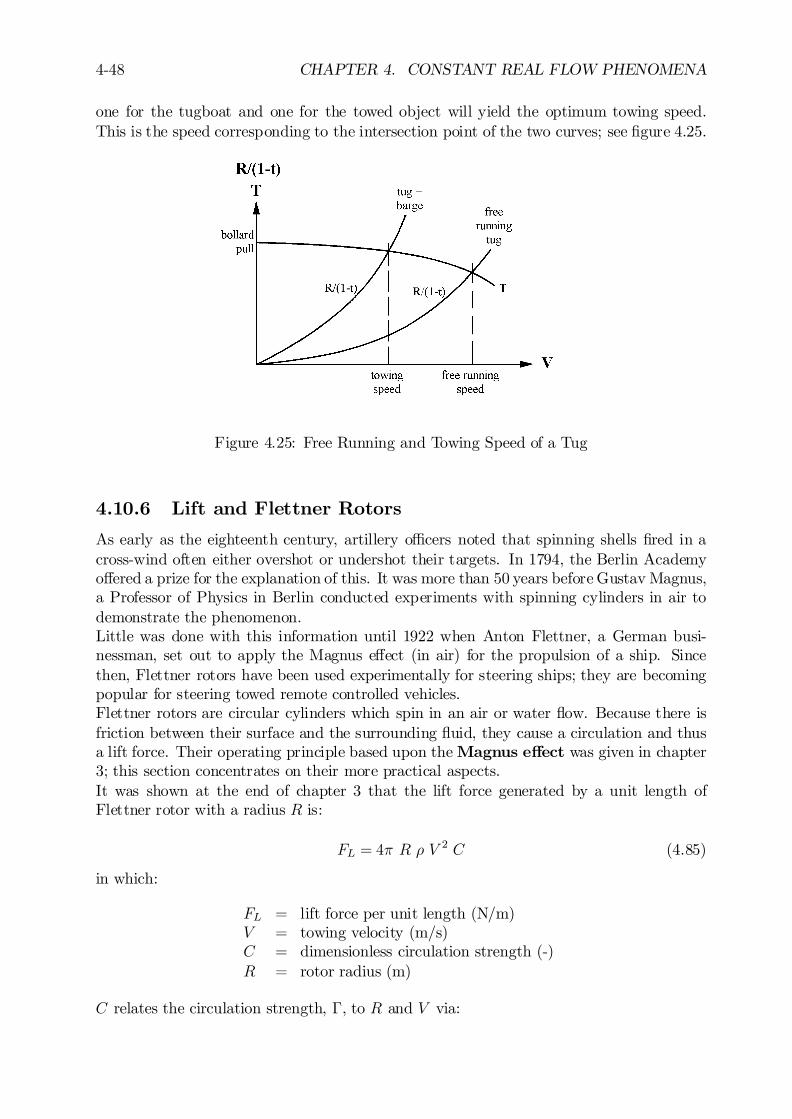
4-48 CHAPTER 4. CONSTANT REAL FLOW PHENOMENA
one for the tugboat and one for the towed object will yield the optimum towing speed.This is the speed corresponding to the intersection point of the two curves; see …gure 4.25.
Figure 4.25: Free Running and Towing Speed of a Tug
4.10.6 Lift and Flettner Rotors
As early as the eighteenth century, artillery o¢cers noted that spinning shells …red in across-wind often either overshot or undershot their targets. In 1794, the Berlin Academyo¤ered a prize for the explanation of this. It was more than 50 years before Gustav Magnus,a Professor of Physics in Berlin conducted experiments with spinning cylinders in air todemonstrate the phenomenon.Little was done with this information until 1922 when Anton Flettner, a German busi-nessman, set out to apply the Magnus e¤ect (in air) for the propulsion of a ship. Sincethen, Flettner rotors have been used experimentally for steering ships; they are becomingpopular for steering towed remote controlled vehicles.Flettner rotors are circular cylinders which spin in an air or water ‡ow. Because there isfriction between their surface and the surrounding ‡uid, they cause a circulation and thusa lift force. Their operating principle based upon the Magnus e¤ect was given in chapter3; this section concentrates on their more practical aspects.It was shown at the end of chapter 3 that the lift force generated by a unit length ofFlettner rotor with a radius R is:
FL = 4¼ R ½ V2 C (4.85)
in which:
FL = lift force per unit length (N/m)V = towing velocity (m/s)C = dimensionless circulation strength (-)R = rotor radius (m)
C relates the circulation strength, ¡, to R and V via:
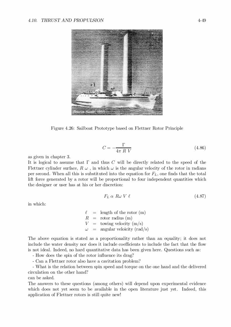
4.10. THRUST AND PROPULSION 4-49
Figure 4.26: Sailboat Prototype based on Flettner Rotor Principle
C = ¡ ¡
4¼ R V(4.86)
as given in chapter 3.It is logical to assume that ¡ and thus C will be directly related to the speed of theFlettner cylinder surface, R ! , in which ! is the angular velocity of the rotor in radiansper second. When all this is substituted into the equation for FL; one …nds that the totallift force generated by a rotor will be proportional to four independent quantities whichthe designer or user has at his or her discretion:
FL ® R! V ` (4.87)
in which:
` = length of the rotor (m)R = rotor radius (m)V = towing velocity (m/s)! = angular veloicity (rad/s)
The above equation is stated as a proportionality rather than an equality; it does notinclude the water density nor does it include coe¢cients to include the fact that the ‡owis not ideal. Indeed, no hard quantitative data has been given here. Questions such as:
- How does the spin of the rotor in‡uence its drag?- Can a Flettner rotor also have a cavitation problem?- What is the relation between spin speed and torque on the one hand and the delivered
circulation on the other hand?can be asked.The answers to these questions (among others) will depend upon experimental evidencewhich does not yet seem to be available in the open literature just yet. Indeed, thisapplication of Flettner rotors is still quite new!
4-50 CHAPTER 4. CONSTANT REAL FLOW PHENOMENA
On a small scale, Flettner rotors are being used in the o¤shore industry to steer RCV’s.On a larger scale, sailboats without sails have even been proposed! This design has largediameter vertical cylinders mounted vertically from the deck instead of masts. They arespun about their vertical axes by motors thus setting up a lift force in the wind much likea spinning tennis ball would. This method of propulsion has not yet proven practical atthis scale, however, although prototypes have been built as shown in …gure 4.26.
Chapter 5
OCEAN SURFACE WAVES
5.1 Introduction
Ocean surface waves cause periodic loads on all sorts of man-made structures in the sea. Itdoes not matter whether these structures are …xed or ‡oating and on the surface or deeperin the sea.Most structures, even the so-called …xed structures, are not really rigid; they respond insome way to the wave-induced periodic loads. Examples of such response include accel-erations, harmonic displacements and internal loads in ships as well as …xed structures.Waves and the resulting ship motions cause added resistance, reduced sustained speed(with associated longer travel times) and increased fuel consumption for ships. Also localerosion near pipelines and other small structures on the sea bed can be caused by waves.The ship’s responses can impair safety via phenomena such as shipping water on deck orwave slamming.In short, there is every reason to need to know about waves - the topic of this chapter- before one goes on with the discussion of all sorts of hydrodynamic problems in laterchapters.
Water waves can be generated in many di¤erent ways:² Waves generated by a ship or any other ‡oating structure which is moving, either at
a constant forward speed or by carrying out an oscillatory motion.² Waves generated by the interaction between wind and the sea surface.² Waves generated by astronomical forces: Tides.² Waves generated by earthquakes or submarine landslides: Tsunamis.² Free surface waves generated in ‡uids in partially …lled tanks; such as fuel or cargo
tanks on a ship.
A single mathematical solution for all problems related to these various types of wavesdoes not exist; even in simple cases approximations are required. It is important to beaware of the limitations of simpli…cations, especially when nonlinear e¤ects can becomeimportant. On the other hand, a simple linear approach can work quite well for manypractical applications.Wind generated waves can be classi…ed into two basic categories: sea and swell. These aredescribed brie‡y here.
0J.M.J. Journée and W.W. Massie, ”OFFSHORE HYDROMECHANICS”, First Edition, January 2001,Delft University of Technology. For updates see web site: http://www.shipmotions.nl.

5-2 CHAPTER 5. OCEAN SURFACE WAVES
² SeaA sea is a train of waves driven by the prevailing local wind …eld. The waves areshort-crested with the lengths of the crests only a few (2-3) times the apparent wavelength. Also, sea waves are very irregular; high waves are followed unpredictablyby low waves and vice versa. Individual wave crests seem to propagate in di¤erentdirections with tens of degrees deviation from the mean direction. The crests arefairly sharp and sometimes even small waves can be observed on these crests or thereare dents in the larger wave crests or troughs. The apparent or virtual wave period,eT , varies continuously, as well as the virtual or apparent wave length, e.
² SwellA swell is waves which have propagated out of the area and local wind in which theywere generated. They are no longer dependent upon the wind and can even propagatefor hundreds of kilometers through areas where the winds are calm. Individual wavesare more regular and the crests are more rounded than those of a sea. The lengthsof the crests are longer, now several (6-7) times the virtual wave length. The waveheight is more predictable, too. If the swell is high, 5 to 6 waves of approximatelyequal heights can pass a given point consecutively. If the waves are low, they canstay low for more than a minute even though the surface elevation remains irregular.
Wind waves, especially, are very irregular. Even so, they can be seen as a superpositionof many simple, regular harmonic wave components, each with its own amplitude, length,period or frequency and direction of propagation. Such a concept can be very handyin many applications; it allows one to predict very complex irregular behavior in termsof much simpler theory of regular waves. This so-called superposition principle, …rstintroduced in hydrodynamics by [St. Denis and Pierson, 1953], is illustrated in …gure 5.1.To analyze complicated wave systems, it is necessary to know the properties of the simpleharmonic components, such as time and location-dependent pressure in the ‡uid, relationbetween wave length and wave period, energy transport, etc.In this respect waves are often classi…ed into two other basic categories:
² Deep water waves, also sometimes referred to as short wavesThe water is considered to be deep if the water depth, h, is more than half the wavelength, ¸, so: h=¸ > 1=2 or ¸=h < 2. These (relatively) short waves do not ’feel’ thesea ‡oor.
² Shallow water waves, also sometimes referred to as long wavesThe water is considered to be shallow if the water depth, h, is less than 1/20 of thewave length, ¸, so: h=¸ < 1=20 or ¸=h > 20. The sea ‡oor has a very large in‡uenceon the characteristics of these (relatively) long waves.
5.2 Regular Waves
De…nitions used to describe the harmonic - or regular - waves and the potential theoryused to solve the ‡ow problem in waves will be treated now.Figure 5.2 shows a harmonic wave as seen from two di¤erent perspectives. Figure 5.2-ashows what one would observe in a snapshot photo made looking at the side of a (trans-parent) wave ‡ume; the wave pro…le is shown as a function of distance x along the ‡umeat a …xed instant in time. Figure 5.2-b is a time record of the water level observed at one
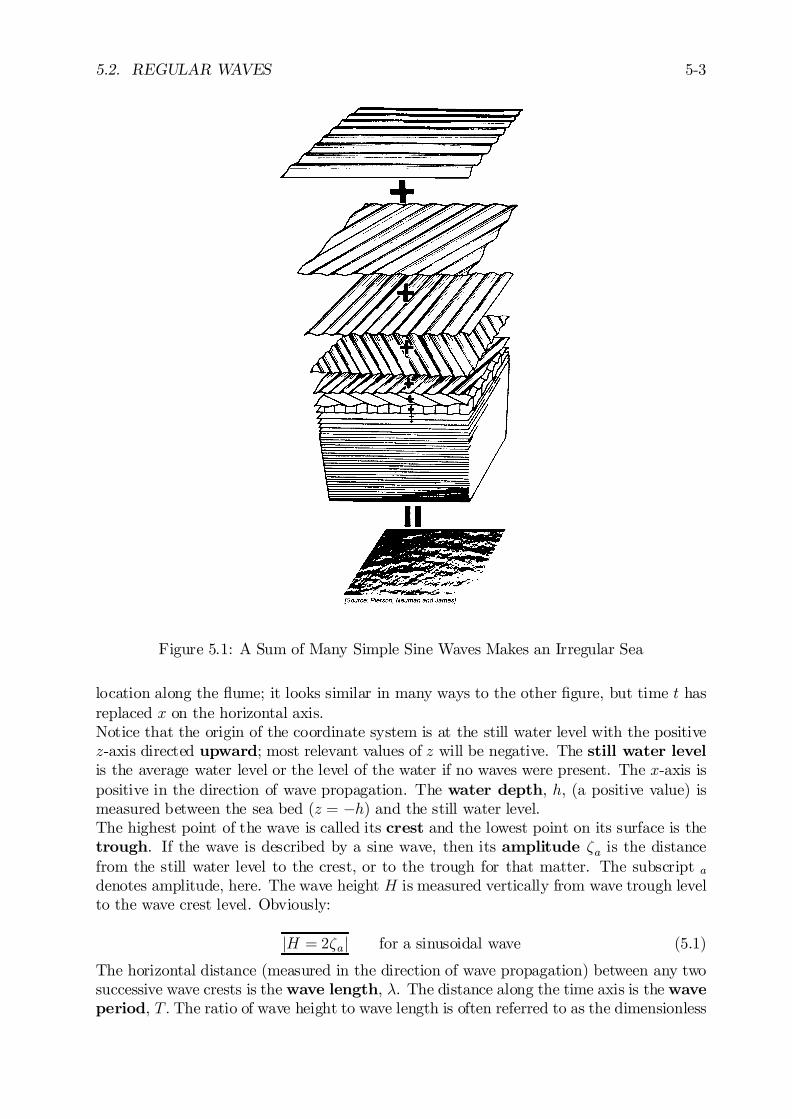
5.2. REGULAR WAVES 5-3
Figure 5.1: A Sum of Many Simple Sine Waves Makes an Irregular Sea
location along the ‡ume; it looks similar in many ways to the other …gure, but time t hasreplaced x on the horizontal axis.Notice that the origin of the coordinate system is at the still water level with the positivez-axis directed upward; most relevant values of z will be negative. The still water levelis the average water level or the level of the water if no waves were present. The x-axis ispositive in the direction of wave propagation. The water depth, h, (a positive value) ismeasured between the sea bed (z = ¡h) and the still water level.The highest point of the wave is called its crest and the lowest point on its surface is thetrough. If the wave is described by a sine wave, then its amplitude ³a is the distancefrom the still water level to the crest, or to the trough for that matter. The subscript a
denotes amplitude, here. The wave height H is measured vertically from wave trough levelto the wave crest level. Obviously:
jH = 2³aj for a sinusoidal wave (5.1)
The horizontal distance (measured in the direction of wave propagation) between any twosuccessive wave crests is the wave length, ¸. The distance along the time axis is the waveperiod, T: The ratio of wave height to wave length is often referred to as the dimensionless
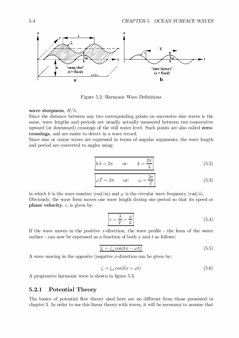
5-4 CHAPTER 5. OCEAN SURFACE WAVES
Figure 5.2: Harmonic Wave De…nitions
wave steepness, H=¸:Since the distance between any two corresponding points on successive sine waves is thesame, wave lengths and periods are usually actually measured between two consecutiveupward (or downward) crossings of the still water level. Such points are also called zero-crossings, and are easier to detect in a wave record.Since sine or cosine waves are expressed in terms of angular arguments, the wave lengthand period are converted to angles using:
¯¯k¸ = 2¼ or: k =
2¼
¸
¯¯ (5.2)
¯¯!T = 2¼ or: ! =
2¼
T
¯¯ (5.3)
in which k is the wave number (rad/m) and ! is the circular wave frequency (rad/s).Obviously, the wave form moves one wave length during one period so that its speed orphase velocity, c, is given by:
¯¯c = ¸
T=!
k
¯¯ (5.4)
If the wave moves in the positive x-direction, the wave pro…le - the form of the watersurface - can now be expressed as a function of both x and t as follows:
j³ = ³a cos(kx¡ !t)j (5.5)
A wave moving in the opposite (negative x-direction can be given by:
³ = ³a cos(kx+ !t) (5.6)
A progressive harmonic wave is shown in …gure 5.3.
5.2.1 Potential Theory
The basics of potential ‡ow theory used here are no di¤erent from those presented inchapter 3. In order to use this linear theory with waves, it will be necessary to assume that
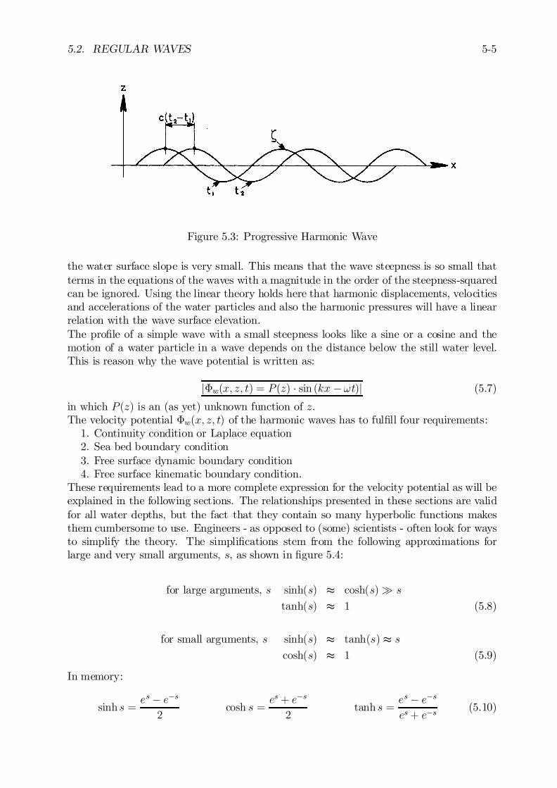
5.2. REGULAR WAVES 5-5
Figure 5.3: Progressive Harmonic Wave
the water surface slope is very small. This means that the wave steepness is so small thatterms in the equations of the waves with a magnitude in the order of the steepness-squaredcan be ignored. Using the linear theory holds here that harmonic displacements, velocitiesand accelerations of the water particles and also the harmonic pressures will have a linearrelation with the wave surface elevation.The pro…le of a simple wave with a small steepness looks like a sine or a cosine and themotion of a water particle in a wave depends on the distance below the still water level.This is reason why the wave potential is written as:
j©w(x; z; t) = P (z) ¢ sin (kx ¡!t)j (5.7)
in which P (z) is an (as yet) unknown function of z.The velocity potential ©w(x; z; t) of the harmonic waves has to ful…ll four requirements:
1. Continuity condition or Laplace equation2. Sea bed boundary condition3. Free surface dynamic boundary condition4. Free surface kinematic boundary condition.
These requirements lead to a more complete expression for the velocity potential as will beexplained in the following sections. The relationships presented in these sections are validfor all water depths, but the fact that they contain so many hyperbolic functions makesthem cumbersome to use. Engineers - as opposed to (some) scientists - often look for waysto simplify the theory. The simpli…cations stem from the following approximations forlarge and very small arguments, s, as shown in …gure 5.4:
for large arguments, s sinh(s) t cosh(s)À s
tanh(s) t 1 (5.8)
for small arguments, s sinh(s) t tanh(s) t s
cosh(s) t 1 (5.9)
In memory:
sinh s =es ¡ e¡s2
cosh s =es+ e¡s
2tanh s =
es ¡ e¡ses+ e¡s
(5.10)
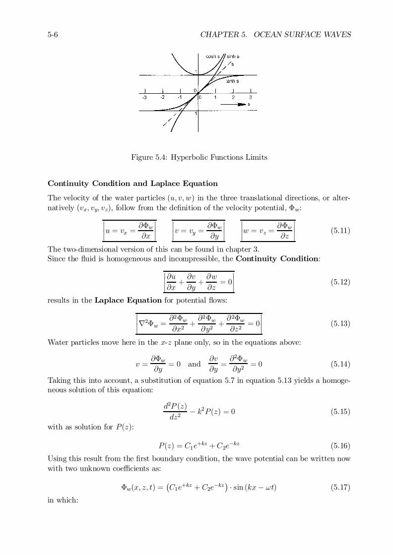
5-6 CHAPTER 5. OCEAN SURFACE WAVES
Figure 5.4: Hyperbolic Functions Limits
Continuity Condition and Laplace Equation
The velocity of the water particles (u; v; w) in the three translational directions, or alter-natively (vx; vy; vz), follow from the de…nition of the velocity potential, ©w:
¯¯u = vx =
@©w@x
¯¯
¯¯v = vy =
@©w@y
¯¯
¯¯w = vz =
@©w@z
¯¯ (5.11)
The two-dimensional version of this can be found in chapter 3.Since the ‡uid is homogeneous and incompressible, the Continuity Condition:
¯¯@u@x+@v
@y+@w
@z= 0
¯¯ (5.12)
results in the Laplace Equation for potential ‡ows:
¯¯r2©w =
@2©w@x2
+@2©w@y2
+@2©w@z2
= 0
¯¯ (5.13)
Water particles move here in the x-z plane only, so in the equations above:
v =@©w@y
= 0 and@v
@y=@2©w@y2
= 0 (5.14)
Taking this into account, a substitution of equation 5.7 in equation 5.13 yields a homoge-neous solution of this equation:
d2P (z)
dz2¡ k2P (z) = 0 (5.15)
with as solution for P (z):
P (z) = C1e+kz +C2e
¡kz (5.16)
Using this result from the …rst boundary condition, the wave potential can be written nowwith two unknown coe¢cients as:
©w(x; z; t) =¡C1e+kz + C2e¡kz
¢¢ sin (kx¡ !t) (5.17)
in which:
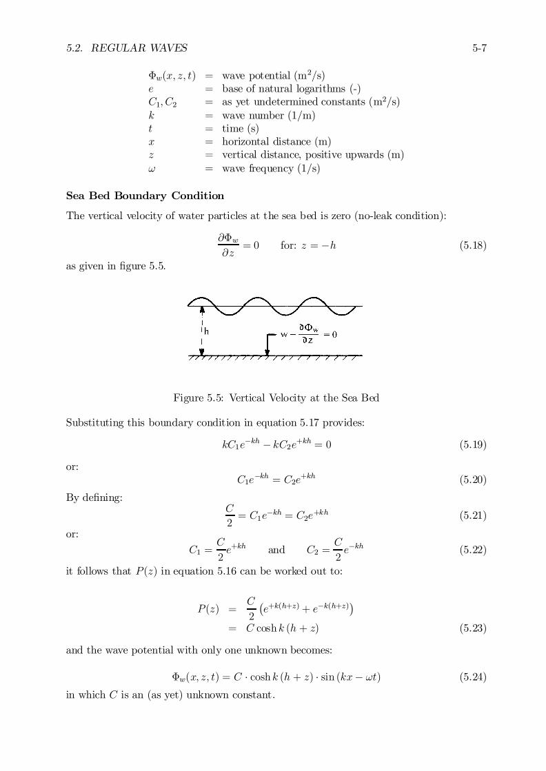
5.2. REGULAR WAVES 5-7
©w(x; z; t) = wave potential (m2/s)e = base of natural logarithms (-)C1; C2 = as yet undetermined constants (m2/s)k = wave number (1/m)t = time (s)x = horizontal distance (m)z = vertical distance, positive upwards (m)! = wave frequency (1/s)
Sea Bed Boundary Condition
The vertical velocity of water particles at the sea bed is zero (no-leak condition):
@©w@z
= 0 for: z = ¡h (5.18)
as given in …gure 5.5.
Figure 5.5: Vertical Velocity at the Sea Bed
Substituting this boundary condition in equation 5.17 provides:
kC1e¡kh ¡ kC2e+kh = 0 (5.19)
or:C1e
¡kh = C2e+kh (5.20)
By de…ning:C
2= C1e
¡kh = C2e+kh (5.21)
or:
C1 =C
2e+kh and C2 =
C
2e¡kh (5.22)
it follows that P (z) in equation 5.16 can be worked out to:
P (z) =C
2
¡e+k(h+z)+ e¡k(h+z)
¢
= C coshk (h + z) (5.23)
and the wave potential with only one unknown becomes:
©w(x; z; t) = C ¢ coshk (h + z) ¢ sin (kx¡ !t) (5.24)
in which C is an (as yet) unknown constant.
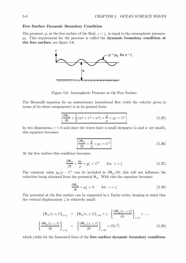
5-8 CHAPTER 5. OCEAN SURFACE WAVES
Free Surface Dynamic Boundary Condition
The pressure, p, at the free surface of the ‡uid, z = ³, is equal to the atmospheric pressure,p0. This requirement for the pressure is called the dynamic boundary condition atthe free surface, see …gure 5.6.
Figure 5.6: Atmospheric Pressure at the Free Surface
The Bernoulli equation for an unstationary irrotational ‡ow (with the velocity given interms of its three components) is in its general form:
¯¯@©w@t
+1
2(u2 + v2 +w2) +
p
½+ gz = C¤
¯¯ (5.25)
In two dimensions, v = 0 and since the waves have a small steepness (u and w are small),this equation becomes:
¯¯@©w@t
+p
½+ gz = C ¤
¯¯ (5.26)
At the free surface this condition becomes:
@©w@t
+p0½+ g³ = C¤ for: z = ³ (5.27)
The constant value p0=½ ¡ C¤ can be included in @©w=@t; this will not in‡uence thevelocities being obtained from the potential ©w. With this the equation becomes:
@©w@t
+ g³ = 0 for: z = ³ (5.28)
The potential at the free surface can be expanded in a Taylor series, keeping in mind thatthe vertical displacement ³ is relatively small:
f©w(x; z; t)gz=³ = f©w(x; z; t)gz=0 + ³ ¢½@©w(x; z; t)
@z
¾
z=0
+ ::::::
½@©w(x; z; t)
@t
¾
z=³
=
½@©w(x; z; t)
@t
¾
z=0
+ O("2) (5.29)
which yields for the linearized form of the free surface dynamic boundary condition:
5.2. REGULAR WAVES 5-9
¯¯@©w@t
+ g³ = 0 for: z = 0
¯¯ (5.30)
With this, the wave pro…le becomes:
³ = ¡1g
¢ @©w@t
for: z = 0 (5.31)
A substitution of equation 5.24 in equation 5.31 yields the wave pro…le:
³ =!C
g¢ cosh kh ¢ cos (kx¡ !t) (5.32)
or:
³ = ³a ¢ cos (kx¡ !t) with: ³a =!C
g¢ coshkh (5.33)
With this the corresponding wave potential, depending on the water depth h, is given bythe relation: ¯
¯©w =³ag
!¢ coshk(h + z)
coshkh¢ sin(kx ¡ !t)
¯¯ (5.34)
In deep water with h ! 1 (short waves), the wave potential becomes:
©w =³ag
!¢ ekz ¢ sin(kx ¡ !t) (deep water) (5.35)
Free Surface Kinematic Boundary Condition
So far the relation between the wave period T and the wave length, ¸, is still unknown.The relation between T and ¸ (or equivalently! and k) follows from the boundary conditionthat the vertical velocity of a water particle at the free surface of the ‡uid is identical to thevertical velocity of that free surface itself (no-leak condition); this is a kinematic boundarycondition.Using the equation of the free surface 5.33 yields for the wave surface:
dz
dt=
@³
@t+@³
@x¢ dxdt
for: z = ³
=@³
@t+ u ¢ d³
dx(5.36)
The second term in this expression is a product of two values, which are both small becauseof the assumed small wave steepness. This product becomes even smaller (second order)and can be ignored, see …gure 5.7.This linearization provides the vertical velocity of the wave surface:
dz
dt=@³
@tfor: z = ³ (5.37)
The vertical velocity of a water particle in the free surface is then:
@©w@z
=@³
@tfor: z = ³ (5.38)

5-10 CHAPTER 5. OCEAN SURFACE WAVES
Figure 5.7: Kinematic Boundary Condition
Analogous to equation 5.30 this condition is valid for z = 0 too, instead of for z = ³ only.A di¤erentiation of the free surface dynamic boundary condition (equation 5.30) withrespect to t provides:
@2©w@t2
+ g@³
@t= 0 for z = 0 (5.39)
or after re-arranging terms:
@³
@t+1
g¢ @
2©w@t2
= 0 for z = 0 (5.40)
Together with equation 5.37 this delivers the free surface kinematic boundary condi-tion or the Cauchy-Poisson condition:
¯¯@z@t+1
g¢ @
2©w@t2
= 0 for: z = 0
¯¯ (5.41)
Dispersion Relationship
The information is now available to establish the relationship between ! and k (or equiva-lently T and ¸) referred to above. A substitution of the expression for the wave potential(equation 5.34) in equation 5.41 gives the dispersion relation for any arbitrary waterdepth h:
j!2 = k g ¢ tanh khj (5.42)
In many situations, ! or T will be know; one must determine k or ¸: Since k appears in anonlinear way in 5.42, that equation will generally have to be solved iteratively.In deep water (tanhkh = 1), equation 5.42 degenerates to a quite simple form which canbe used without di¢culty:
!2 = k g (deep water) (5.43)
and the deep water relation between T and ¸ becomes:
T =
r2¼
g¢p¸ or ¸ =
g
2¼¢T 2 (deep water) (5.44)
5.2. REGULAR WAVES 5-11
Substitution of g = 9:81 m/s2 and ¼ yields:
T t 0:80 ¢p¸ or ¸ t 1:56 ¢ T 2 (deep water) (5.45)
Note that this regular wave relation cannot be used to describe the relation between theaverage wave length and the average wave period of an irregular sea. However in a moreregular swell, this relation can be used with an accuracy of about 10 to 15 per cent.In shallow water, the dispersion relation is found by substituting tanhkh = kh in equa-tion 5.42; thus:
! = k ¢pgh (shallow water) (5.46)
and the shallow water relation between T and ¸ becomes:
T =¸pgh
or ¸ = T ¢pgh (shallow water) (5.47)
Cauchy-Poisson Condition in Deep Water
In deep water (short waves), the free surface kinematic boundary condition orCauchy-Poisson condition is often given in another form in the literature. The space andtime dependent wave potential, ©w(x; z; t), is divided in a space-dependent part, Áw(x; z),and a time-dependent part, 1 ¢ sin !t, by de…ning:
©w(x; z; t) = Áw(x; z) ¢ sin!t (5.48)
Equation 5.41:
@z
@t+1
g¢ @
2©w@t2
= 0 for: z = 0
can with equation 5.37 be written as:
@³
@t+1
g¢ @
2©w@t2
= 0 for: z = 0 (5.49)
and using equation 5.38 results in:
@©w@z
+1
g¢ @
2©w@t2
= 0 for: z = 0 (5.50)
With the dispersion relation in deep water, !2 = k g; the free surface kinematic boundarycondition or the Cauchy-Poisson condition becomes:
@Áw@z
¡ k ¢ Áw = 0 for z = 0 (deep water) (5.51)
5.2.2 Phase Velocity
With the dispersion relation (equation 5.42) the wave celerity (c = ¸=T = !=k) becomes:
¯¯c =
rg
k¢ tanh kh
¯¯ (5.52)
5-12 CHAPTER 5. OCEAN SURFACE WAVES
The phase velocity increases with the wave length (k = 2¼=¸); water waves display disper-sion in that longer waves move faster than shorter ones. As a result of this phenomena, seasailors often interpret swell (long, relatively low wind-generated waves which have movedaway from the storm that generated them) as a warning of an approaching storm.In deep water, the phase velocity is found by substituting tanhkh = 1 in equation 5.52;thus:
c =
rg
k=g
!(deep water) (5.53)
With some further substitution, one can get:
c =
rg
k=
rg ¢ ¸2¼=
rg
2¼¢ ¸ t 1:25
p¸ t 1:56 ¢ T (deep water) (5.54)
In shallow water, the phase velocity is found by substituting tanhkh = kh in equation5.52; thus:
c =pgh (shallow water) (5.55)
The phase velocity is now independent of the wave period; these waves are not dispersive.This celerity,
pgh, is called the critical velocity. This velocity is of importance when
sailing with a ship at shallow water. Similar e¤ects occur with an airplane that exceedsthe speed of sound. Generally, the forward ship speed will be limited to about 80% of thecritical velocity, to avoid excessive still water resistance or squat (combined sinkage andtrim). Indeed, only a ship which can plane on the water surface is able to move faster thanthe wave which it generates.
5.2.3 Water Particle Kinematics
The kinematics of a water particle is found from the velocity components in the x- andz-directions, obtained from the velocity potential given in equation 5.34 and the dispersionrelation given in equation 5.42.
Velocities
The resulting velocity components - in their most general form - can be expressed as:
u =@©w@x
=dx
dt= ³a ¢ kg
!¢ coshk (h+ z)
coshkh¢ cos (kx ¡ !t)
w =@©w@z
=dz
dt= ³a ¢ kg
!¢ sinhk (h+ z)
coshkh¢ sin (kx ¡ !t) (5.56)
A substitution of:
kg =!2
tanhkh
derived from the dispersion relation in equation 5.42, provides:
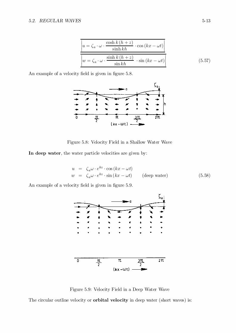
5.2. REGULAR WAVES 5-13
¯¯u = ³a ¢ ! ¢ cosh k (h + z)
sinhkh¢ cos (kx¡ !t)
¯¯
¯¯w = ³a ¢ ! ¢ sinh k (h + z)
sinkh¢ sin (kx ¡ !t)
¯¯ (5.57)
An example of a velocity …eld is given in …gure 5.8.
Figure 5.8: Velocity Field in a Shallow Water Wave
In deep water, the water particle velocities are given by:
u = ³a! ¢ ekz ¢ cos (kx¡ !t)w = ³a! ¢ ekz ¢ sin (kx ¡ !t) (deep water) (5.58)
An example of a velocity …eld is given in …gure 5.9.
Figure 5.9: Velocity Field in a Deep Water Wave
The circular outline velocity or orbital velocity in deep water (short waves) is:
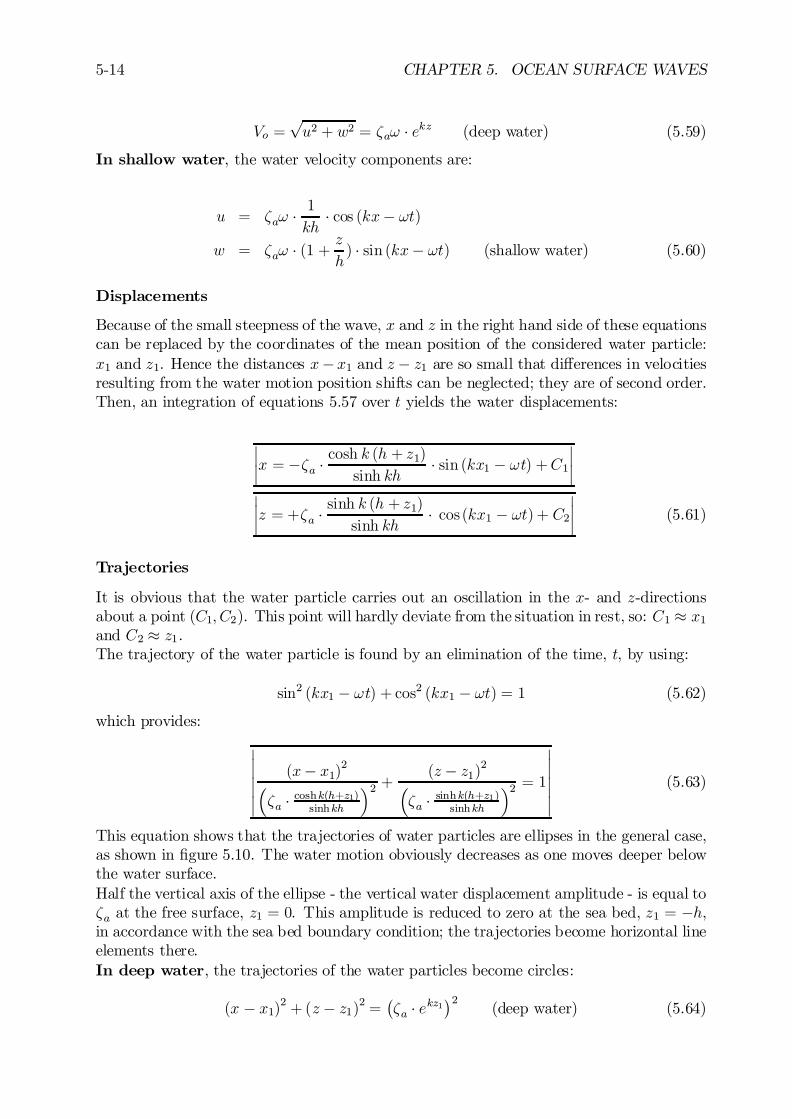
5-14 CHAPTER 5. OCEAN SURFACE WAVES
Vo =pu2 + w2 = ³a! ¢ ekz (deep water) (5.59)
In shallow water, the water velocity components are:
u = ³a! ¢ 1kh
¢ cos (kx¡ !t)
w = ³a! ¢ (1 + zh) ¢ sin (kx¡ !t) (shallow water) (5.60)
Displacements
Because of the small steepness of the wave, x and z in the right hand side of these equationscan be replaced by the coordinates of the mean position of the considered water particle:x1 and z1. Hence the distances x¡x1 and z ¡ z1 are so small that di¤erences in velocitiesresulting from the water motion position shifts can be neglected; they are of second order.Then, an integration of equations 5.57 over t yields the water displacements:
¯¯x = ¡³a ¢ cosh k (h + z1)
sinh kh¢ sin (kx1 ¡ !t) +C1
¯¯
¯¯z = +³a ¢ sinh k (h + z1)
sinh kh¢ cos(kx1 ¡ !t) + C2
¯¯ (5.61)
Trajectories
It is obvious that the water particle carries out an oscillation in the x- and z-directionsabout a point (C1; C2). This point will hardly deviate from the situation in rest, so: C1 ¼ x1and C2 ¼ z1.The trajectory of the water particle is found by an elimination of the time, t, by using:
sin2 (kx1 ¡ !t) + cos2 (kx1 ¡ !t) = 1 (5.62)
which provides:
¯¯¯¯
(x¡ x1)2³³a ¢ coshk(h+z1)
sinhkh
´2 +(z ¡ z1)2³
³a ¢ sinhk(h+z1)sinhkh
´2 = 1
¯¯¯¯
(5.63)
This equation shows that the trajectories of water particles are ellipses in the general case,as shown in …gure 5.10. The water motion obviously decreases as one moves deeper belowthe water surface.Half the vertical axis of the ellipse - the vertical water displacement amplitude - is equal to³a at the free surface, z1 = 0. This amplitude is reduced to zero at the sea bed, z1 = ¡h,in accordance with the sea bed boundary condition; the trajectories become horizontal lineelements there.In deep water, the trajectories of the water particles become circles:
(x ¡ x1)2 + (z ¡ z1)2 =¡³a ¢ ekz1
¢2(deep water) (5.64)
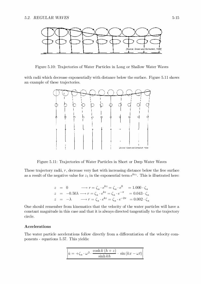
5.2. REGULAR WAVES 5-15
Figure 5.10: Trajectories of Water Particles in Long or Shallow Water Waves
with radii which decrease exponentially with distance below the surface. Figure 5.11 showsan example of these trajectories.
Figure 5.11: Trajectories of Water Particles in Short or Deep Water Waves
These trajectory radii, r, decrease very fast with increasing distance below the free surfaceas a result of the negative value for z1 in the exponential term ekz1. This is illustrated here:
z = 0 ¡! r = ³a ¢ ekz = ³a ¢ e0 = 1:000 ¢ ³az = ¡0:50¸ ¡! r = ³a ¢ ekz = ³a ¢ e¡¼ = 0:043 ¢ ³az = ¡¸ ¡! r = ³a ¢ ekz = ³a ¢ e¡2¼ = 0:002 ¢ ³a
One should remember from kinematics that the velocity of the water particles will have aconstant magnitude in this case and that it is always directed tangentially to the trajectorycircle.
Accelerations
The water particle accelerations follow directly from a di¤erentiation of the velocity com-ponents - equations 5.57. This yields:
¯¯ _u = +³a ¢ !2 ¢ coshk (h+ z)
sinhkh¢ sin (kx ¡!t)
¯¯
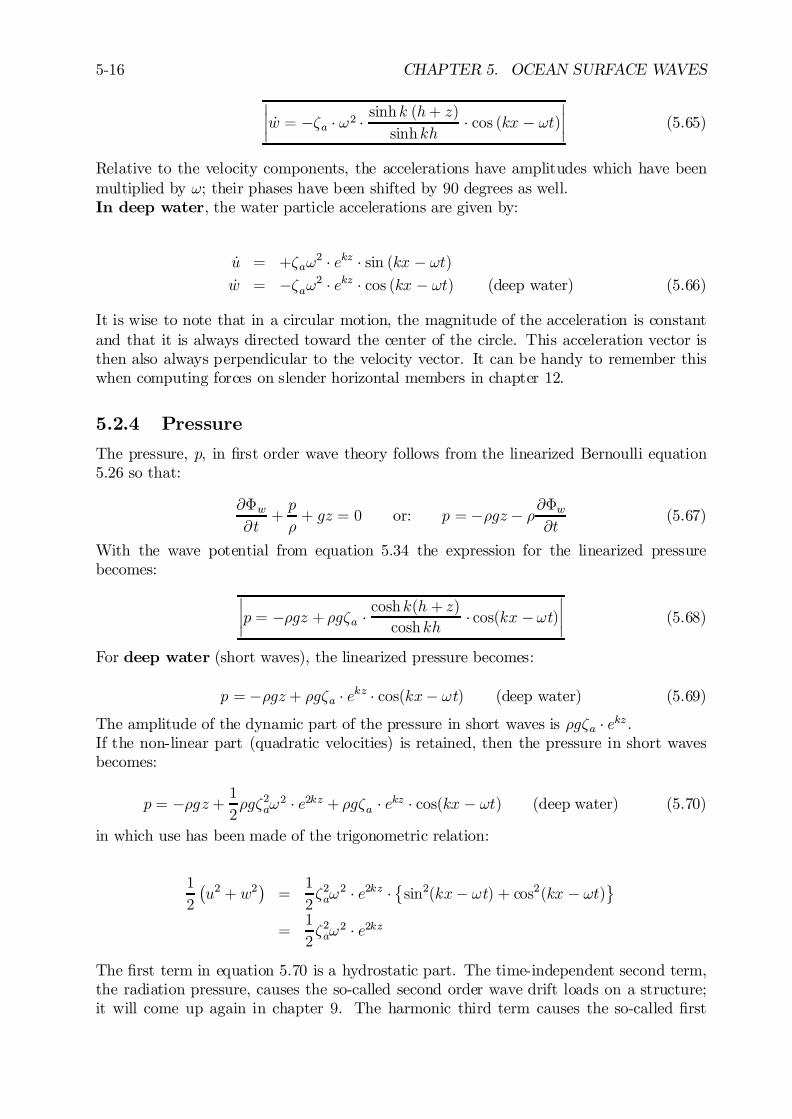
5-16 CHAPTER 5. OCEAN SURFACE WAVES
¯¯ _w = ¡³a ¢ !2 ¢ sinhk (h+ z)
sinhkh¢ cos (kx ¡ !t)
¯¯ (5.65)
Relative to the velocity components, the accelerations have amplitudes which have beenmultiplied by !; their phases have been shifted by 90 degrees as well.In deep water, the water particle accelerations are given by:
_u = +³a!2 ¢ ekz ¢ sin (kx ¡ !t)
_w = ¡³a!2 ¢ ekz ¢ cos (kx ¡ !t) (deep water) (5.66)
It is wise to note that in a circular motion, the magnitude of the acceleration is constantand that it is always directed toward the center of the circle. This acceleration vector isthen also always perpendicular to the velocity vector. It can be handy to remember thiswhen computing forces on slender horizontal members in chapter 12.
5.2.4 Pressure
The pressure, p, in …rst order wave theory follows from the linearized Bernoulli equation5.26 so that:
@©w@t
+p
½+ gz = 0 or: p = ¡½gz ¡ ½@©w
@t(5.67)
With the wave potential from equation 5.34 the expression for the linearized pressurebecomes:
¯¯p = ¡½gz + ½g³a ¢ coshk(h + z)
coshkh¢ cos(kx ¡!t)
¯¯ (5.68)
For deep water (short waves), the linearized pressure becomes:
p = ¡½gz + ½g³a ¢ ekz ¢ cos(kx¡ !t) (deep water) (5.69)
The amplitude of the dynamic part of the pressure in short waves is ½g³a ¢ ekz .If the non-linear part (quadratic velocities) is retained, then the pressure in short wavesbecomes:
p = ¡½gz + 12½g³2a!
2 ¢ e2kz + ½g³a ¢ ekz ¢ cos(kx ¡ !t) (deep water) (5.70)
in which use has been made of the trigonometric relation:
1
2
¡u2 + w2
¢=
1
2³2a!
2 ¢ e2kz ¢©sin2(kx¡ !t) + cos2(kx ¡ !t)
ª
=1
2³2a!
2 ¢ e2kz
The …rst term in equation 5.70 is a hydrostatic part. The time-independent second term,the radiation pressure, causes the so-called second order wave drift loads on a structure;it will come up again in chapter 9. The harmonic third term causes the so-called …rst
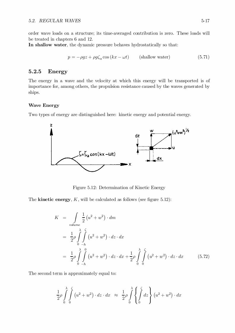
5.2. REGULAR WAVES 5-17
order wave loads on a structure; its time-averaged contribution is zero. These loads willbe treated in chapters 6 and 12.In shallow water, the dynamic pressure behaves hydrostatically so that:
p = ¡½gz + ½g³a cos (kx¡ !t) (shallow water) (5.71)
5.2.5 Energy
The energy in a wave and the velocity at which this energy will be transported is ofimportance for, among others, the propulsion resistance caused by the waves generated byships.
Wave Energy
Two types of energy are distinguished here: kinetic energy and potential energy.
Figure 5.12: Determination of Kinetic Energy
The kinetic energy, K , will be calculated as follows (see …gure 5.12):
K =
Z
volume
1
2
¡u2 + w2
¢¢ dm
=1
2½
¸Z
0
³Z
¡h
¡u2 + w2
¢¢ dz ¢ dx
=1
2½
¸Z
0
0Z
¡h
¡u2 + w2
¢¢ dz ¢ dx + 1
2½
¸Z
0
³Z
0
¡u2 + w2
¢¢ dz ¢ dx (5.72)
The second term is approximately equal to:
1
2½
¸Z
0
³Z
0
¡u2 + w2
¢¢ dz ¢ dx ¼ 1
2½
¸Z
0
8<:
³Z
0
dz
9=;
¡u2 + w2
¢¢ dx

5-18 CHAPTER 5. OCEAN SURFACE WAVES
=1
2½³
¸Z
0
¡u2 + w2
¢¢ dx (5.73)
which is of second order - relative to the …rst term in equation 5.72 - and can be ignored.In a linearized form this equation then becomes:
K =1
2½
¸Z
0
0Z
¡h
¡u2 + w2
¢¢ dz ¢ dx (5.74)
A substitution of the expressions for u and w from equation 5.57 and using the dispersionrelation of equation 5.42 and some algebra provides:
K =1
4½g³2a ¢ ¸ per unit width (crest length)
=1
4½g³2a per unit horizontal sea surface area (5.75)
Some trigonometric relations have been used to obtain these results:
0Z
¡h
sinh2 k (h+ z) ¢ dz =1
4ksinh2kh¡ 1
2h
0Z
¡h
cosh2 k (h+ z) ¢ dz =1
4ksinh2kh+
1
2h
¸Z
0
sin2(kx¡ !t) ¢ dx =
¸Z
0
cos2(kx¡ !t) ¢ dx = 12¸ (5.76)
Figure 5.13: Determination of Potential Energy
The potential energy, P , will be calculated as follows (see …gure 5.13):
P =1
2
¸Z
0
½g³2 ¢ dx

5.2. REGULAR WAVES 5-19
=1
2½g³2a
¸Z
0
cos2(kx¡ !t) ¢ dx (5.77)
Some algebra results in:
P =1
4½g³2a ¢ ¸ per unit width (crest length)
=1
4½g³2a per unit horizontal sea surface area (5.78)
This has the same magnitude as the kinetic energy.The total wave energy, E , follows from equations 5.75 and 5.78, E =K + P :
¯¯E = 1
2½g³2a =
1
8½gH2 per unit horizontal sea surface area
¯¯ (5.79)
Energy Transport or Power
The velocity at which the wave energy will be transported can be determined using …gure5.14. It shows a virtual vertical plane AA0, which is perpendicular to the direction ofpropagation of the wave. An element in this plane (shaded in …gure 5.14) is of unit widthand has height dz:
Figure 5.14: Wave Energy Transport
When the ‡uid passes through this plane element, a certain amount work dW will bedelivered in a direction against the pressure p of the ‡uid.The work done is force times distance:
dW = fp ¢ 1 ¢ dzg ¢ fu ¢ dtg (5.80)
The average work done over one period, T , or power is after linearization:

5-20 CHAPTER 5. OCEAN SURFACE WAVES
W =1
T
t+TZ
t
0Z
¡h
p ¢ u ¢ dz ¢ dt (5.81)
which follows if one realizes that the contribution from the uppermost segment - the splashzone - can be neglected:
1
T
t+TZ
t
³Z
0
p ¢ u ¢ dz ¢ dt ¼ 0 (5.82)
Substituting 5.71 for the pressure and 5.57 for u results in:
W = ¡ ½kg2³aT ¢ ! ¢ sinhkh
t+TZ
t
0Z
¡h
z ¢ coshk (h + z) ¢ cos (kx ¡ !t) ¢ dz ¢ dt
+½kg2³2a
T ¢ ! ¢ sinh kh ¢ coshkh
t+TZ
t
0Z
¡h
cosh2 k(h + z) ¢ cos2 (kx¡ !t) ¢ dz ¢ dt (5.83)
The …rst term is zero and, with the relations given in equations 5.76, the average workdone or power becomes:
W =½g³2a!
sinh2kh¢µ1
4ksinh2kh+
1
2h
¶(5.84)
With c = !=k, this relation becomes:
¯¯W =
1
2½g³2a ¢ c
2¢µ1 +
2kh
sinh2kh
¶¯¯ (5.85)
or in terms of wave height:
W =1
8½gH2 ¢ c
2¢µ1 +
2kh
sinh2kh
¶(5.86)
Group Velocity
The average work done per wave period in equation 5.85 can also be written as:
W = E ¢ cg (5.87)
with:
E =1
2½g³2a =
1
8½gH2
¯¯cg =
c
2¢µ1 +
2kh
sinh 2kh
¶¯¯ (5.88)
Then E is the energy of the waves per unit area and cg is the velocity at which this energywill be transported in the waves, the wave group velocity.
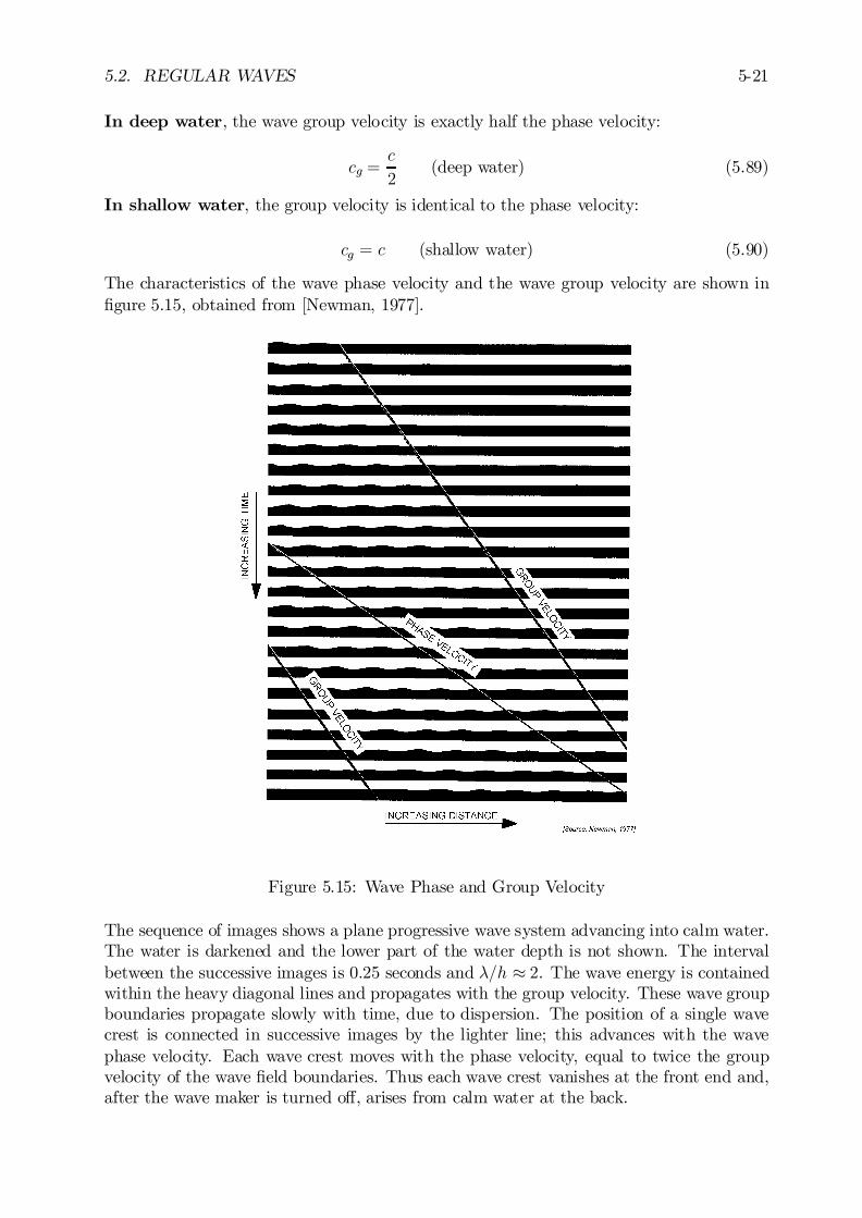
5.2. REGULAR WAVES 5-21
In deep water, the wave group velocity is exactly half the phase velocity:
cg =c
2(deep water) (5.89)
In shallow water, the group velocity is identical to the phase velocity:
cg = c (shallow water) (5.90)
The characteristics of the wave phase velocity and the wave group velocity are shown in…gure 5.15, obtained from [Newman, 1977].
Figure 5.15: Wave Phase and Group Velocity
The sequence of images shows a plane progressive wave system advancing into calm water.The water is darkened and the lower part of the water depth is not shown. The intervalbetween the successive images is 0.25 seconds and ¸=h ¼ 2. The wave energy is containedwithin the heavy diagonal lines and propagates with the group velocity. These wave groupboundaries propagate slowly with time, due to dispersion. The position of a single wavecrest is connected in successive images by the lighter line; this advances with the wavephase velocity. Each wave crest moves with the phase velocity, equal to twice the groupvelocity of the wave …eld boundaries. Thus each wave crest vanishes at the front end and,after the wave maker is turned o¤, arises from calm water at the back.
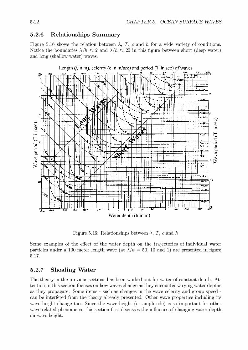
5-22 CHAPTER 5. OCEAN SURFACE WAVES
5.2.6 Relationships Summary
Figure 5.16 shows the relation between ¸, T , c and h for a wide variety of conditions.Notice the boundaries ¸=h ¼ 2 and ¸=h ¼ 20 in this …gure between short (deep water)and long (shallow water) waves.
Figure 5.16: Relationships between ¸, T , c and h
Some examples of the e¤ect of the water depth on the trajectories of individual waterparticles under a 100 meter length wave (at ¸=h = 50, 10 and 1) are presented in …gure5.17.
5.2.7 Shoaling Water
The theory in the previous sections has been worked out for water of constant depth. At-tention in this section focuses on how waves change as they encounter varying water depthsas they propagate. Some items - such as changes in the wave celerity and group speed -can be interfered from the theory already presented. Other wave properties including itswave height change too. Since the wave height (or amplitude) is so important for otherwave-related phenomena, this section …rst discusses the in‡uence of changing water depthon wave height.
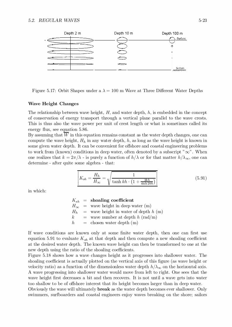
5.2. REGULAR WAVES 5-23
Figure 5.17: Orbit Shapes under a ¸ = 100 m Wave at Three Di¤erent Water Depths
Wave Height Changes
The relationship between wave height, H; and water depth, h; is embedded in the conceptof conservation of energy transport through a vertical plane parallel to the wave crests.This is thus also the wave power per unit of crest length or what is sometimes called itsenergy ‡ux, see equation 5.86.By assuming thatW in this equation remains constant as the water depth changes, one cancompute the wave height, Hh in any water depth, h; as long as the wave height is known insome given water depth. It can be convenient for o¤shore and coastal engineering problemsto work from (known) conditions in deep water, often denoted by a subscript ”1”. Whenone realizes that k = 2¼=¸ - is purely a function of h=¸ or for that matter h=¸1, one candetermine - after quite some algebra - that:
¯¯¯Ksh =
HhH1
=
s1
tanh kh ¢¡1 + 2kh
sinh2kh
¢¯¯¯ (5.91)
in which:
Ksh = shoaling coe¢cientH1 = wave height in deep water (m)Hh = wave height in water of depth h (m)k = wave number at depth h (rad/m)h = chosen water depth (m)
If wave conditions are known only at some …nite water depth, then one can …rst useequation 5.91 to evaluate Ksh at that depth and then compute a new shoaling coe¢cientat the desired water depth. The known wave height can then be transformed to one at thenew depth using the ratio of the shoaling coe¢cients.Figure 5.18 shows how a wave changes height as it progresses into shallower water. Theshoaling coe¢cient is actually plotted on the vertical axis of this …gure (as wave height orvelocity ratio) as a function of the dimensionless water depth h=¸1 on the horizontal axis.A wave progressing into shallower water would move from left to right. One sees that thewave height …rst decreases a bit and then recovers. It is not until a wave gets into watertoo shallow to be of o¤shore interest that its height becomes larger than in deep water.Obviously the wave will ultimately break as the water depth becomes ever shallower. Onlyswimmers, surfboarders and coastal engineers enjoy waves breaking on the shore; sailors
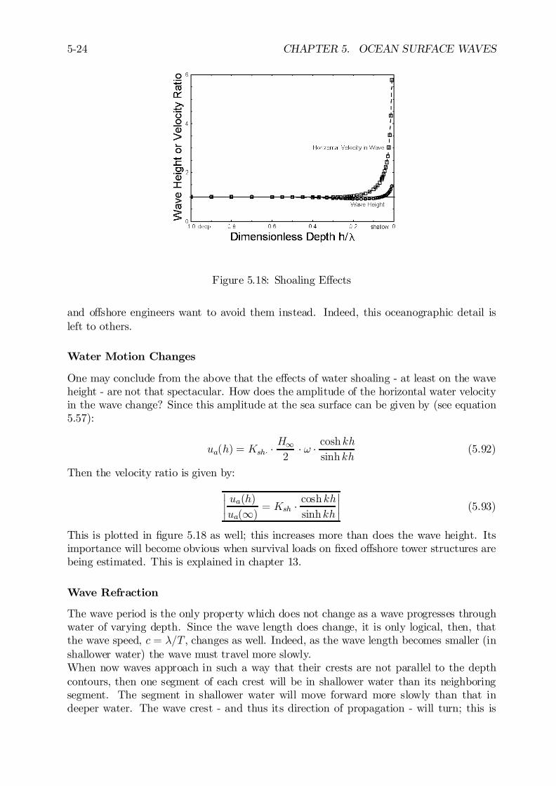
5-24 CHAPTER 5. OCEAN SURFACE WAVES
Figure 5.18: Shoaling E¤ects
and o¤shore engineers want to avoid them instead. Indeed, this oceanographic detail isleft to others.
Water Motion Changes
One may conclude from the above that the e¤ects of water shoaling - at least on the waveheight - are not that spectacular. How does the amplitude of the horizontal water velocityin the wave change? Since this amplitude at the sea surface can be given by (see equation5.57):
ua(h) = Ksh¢ ¢H12
¢ ! ¢ coshkhsinhkh
(5.92)
Then the velocity ratio is given by:
¯¯ ua(h)ua(1)
= Ksh ¢ coshkhsinhkh
¯¯ (5.93)
This is plotted in …gure 5.18 as well; this increases more than does the wave height. Itsimportance will become obvious when survival loads on …xed o¤shore tower structures arebeing estimated. This is explained in chapter 13.
Wave Refraction
The wave period is the only property which does not change as a wave progresses throughwater of varying depth. Since the wave length does change, it is only logical, then, thatthe wave speed, c = ¸=T , changes as well. Indeed, as the wave length becomes smaller (inshallower water) the wave must travel more slowly.When now waves approach in such a way that their crests are not parallel to the depthcontours, then one segment of each crest will be in shallower water than its neighboringsegment. The segment in shallower water will move forward more slowly than that indeeper water. The wave crest - and thus its direction of propagation - will turn; this is

5.2. REGULAR WAVES 5-25
called refraction much like the similar phenomena with light in physics. The wave crestsalways turn in such a way that their crests become more parallel to the depth contours asthey proceed into shallower water.
5.2.8 Wave Re‡ection and Di¤raction
When a regular wave component meets a vertical wall perpendicular to its propagationdirection - such as the side of a big ship - it is re‡ected and sent back where it came fromwith (ideally) an identical amplitude and speed. The water surface near the ship appearsto move up and down - with twice the amplitude of the incoming wave - but there is noapparent wave progression. This describes a standing wave, which can be formulated byadding up two identical waves moving in opposite directions as given in equations 5.94.
³ = ³1 + ³2= ³a cos (kx ¡ !t) + ³a cos (kx+ !t)= 2³a cos(kx) cos (!t) (5.94)
The amplitude of this resulting wave is twice the amplitude of the two separate progressivewave components and the phase velocity becomes zero; see …gures 5.19 and 5.20.
Figure 5.19: Standing Wave
Figure 5.20: Fluid Motions under a Standing Wave
If the wave approaches the wall under an angle, then the above approach is still valid forits component perpendicular to the wall. The wave is re‡ected away from the wall at anangle in the same as light re‡ects from a ‡at mirror.Wave di¤raction is a process by which wave energy is propagated into a shadow zone- an area which is not directly in line with the approaching wave. Coastal engineers use
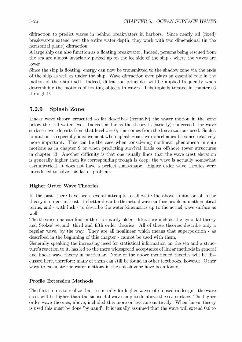
5-26 CHAPTER 5. OCEAN SURFACE WAVES
di¤raction to predict waves in behind breakwaters in harbors. Since nearly all (…xed)breakwaters extend over the entire water depth, they work with two dimensional (in thehorizontal plane) di¤raction.A large ship can also function as a ‡oating breakwater. Indeed, persons being rescued fromthe sea are almost invariably picked up on the lee side of the ship - where the waves arelower.Since the ship is ‡oating, energy can now be transmitted to the shadow zone via the endsof the ship as well as under the ship. Wave di¤raction even plays an essential role in themotion of the ship itself. Indeed, di¤raction principles will be applied frequently whendetermining the motions of ‡oating objects in waves. This topic is treated in chapters 6through 9.
5.2.9 Splash Zone
Linear wave theory presented so far describes (formally) the water motion in the zonebelow the still water level. Indeed, as far as the theory is (strictly) concerned, the wavesurface never departs from that level z = 0; this comes from the linearizations used. Such alimitation is especially inconvenient when splash zone hydromechanics becomes relativelymore important. This can be the case when considering nonlinear phenomena in shipmotions as in chapter 9 or when predicting survival loads on o¤shore tower structuresin chapter 13. Another di¢culty is that one usually …nds that the wave crest elevationis generally higher than its corresponding trough is deep; the wave is actually somewhatasymmetrical, it does not have a perfect sinus-shape. Higher order wave theories wereintroduced to solve this latter problem.
Higher Order Wave Theories
In the past, there have been several attempts to alleviate the above limitation of lineartheory in order - at least - to better describe the actual wave surface pro…le in mathematicalterms, and - with luck - to describe the water kinematics up to the actual wave surface aswell.The theories one can …nd in the - primarily older - literature include the cynoidal theoryand Stokes’ second, third and …fth order theories. All of these theories describe only aregular wave, by the way. They are all nonlinear which means that superposition - asdescribed in the beginning of this chapter - cannot be used with them.Generally speaking the increasing need for statistical information on the sea and a struc-ture’s reaction to it, has led to the more widespread acceptance of linear methods in generaland linear wave theory in particular. None of the above mentioned theories will be dis-cussed here, therefore; many of them can still be found in other textbooks, however. Otherways to calculate the water motions in the splash zone have been found.
Pro…le Extension Methods
The …rst step is to realize that - especially for higher waves often used in design - the wavecrest will be higher than the sinusoidal wave amplitude above the sea surface. The higherorder wave theories, above, included this more or less automatically. When linear theoryis used this must be done ’by hand’. It is usually assumed that the wave will extend 0.6 to
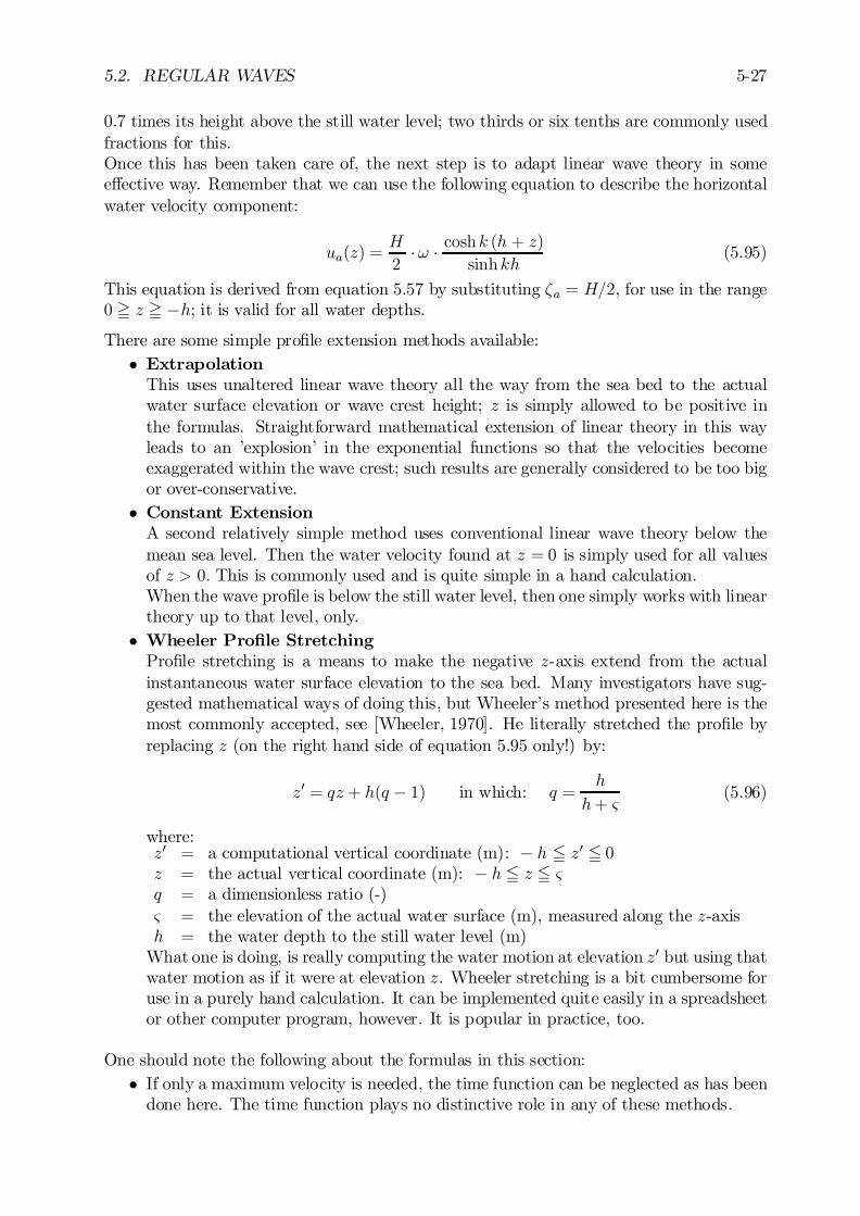
5.2. REGULAR WAVES 5-27
0.7 times its height above the still water level; two thirds or six tenths are commonly usedfractions for this.Once this has been taken care of, the next step is to adapt linear wave theory in somee¤ective way. Remember that we can use the following equation to describe the horizontalwater velocity component:
ua(z) =H
2¢! ¢ coshk (h + z)
sinhkh(5.95)
This equation is derived from equation 5.57 by substituting ³a = H=2, for use in the range0 = z = ¡h; it is valid for all water depths.
There are some simple pro…le extension methods available:² Extrapolation
This uses unaltered linear wave theory all the way from the sea bed to the actualwater surface elevation or wave crest height; z is simply allowed to be positive inthe formulas. Straightforward mathematical extension of linear theory in this wayleads to an ’explosion’ in the exponential functions so that the velocities becomeexaggerated within the wave crest; such results are generally considered to be too bigor over-conservative.
² Constant ExtensionA second relatively simple method uses conventional linear wave theory below themean sea level. Then the water velocity found at z = 0 is simply used for all valuesof z > 0: This is commonly used and is quite simple in a hand calculation.When the wave pro…le is below the still water level, then one simply works with lineartheory up to that level, only.
² Wheeler Pro…le StretchingPro…le stretching is a means to make the negative z-axis extend from the actualinstantaneous water surface elevation to the sea bed. Many investigators have sug-gested mathematical ways of doing this, but Wheeler’s method presented here is themost commonly accepted, see [Wheeler, 1970]. He literally stretched the pro…le byreplacing z (on the right hand side of equation 5.95 only!) by:
z0 = qz + h(q ¡ 1) in which: q =h
h+ &(5.96)
where:z0 = a computational vertical coordinate (m): ¡ h 5 z0 5 0z = the actual vertical coordinate (m): ¡ h 5 z 5 &q = a dimensionless ratio (-)& = the elevation of the actual water surface (m), measured along the z-axish = the water depth to the still water level (m)
What one is doing, is really computing the water motion at elevation z0 but using thatwater motion as if it were at elevation z. Wheeler stretching is a bit cumbersome foruse in a purely hand calculation. It can be implemented quite easily in a spreadsheetor other computer program, however. It is popular in practice, too.
One should note the following about the formulas in this section:² If only a maximum velocity is needed, the time function can be neglected as has been
done here. The time function plays no distinctive role in any of these methods.
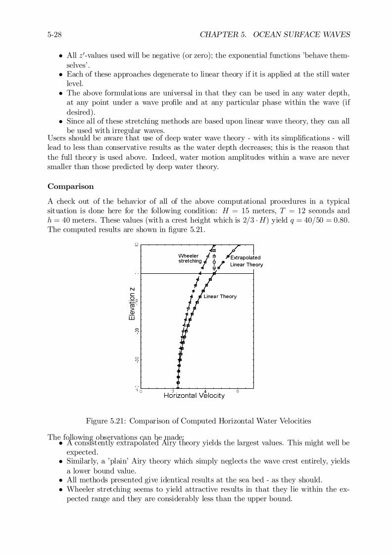
5-28 CHAPTER 5. OCEAN SURFACE WAVES
² All z0-values used will be negative (or zero); the exponential functions ’behave them-selves’.
² Each of these approaches degenerate to linear theory if it is applied at the still waterlevel.
² The above formulations are universal in that they can be used in any water depth,at any point under a wave pro…le and at any particular phase within the wave (ifdesired).
² Since all of these stretching methods are based upon linear wave theory, they can allbe used with irregular waves.
Users should be aware that use of deep water wave theory - with its simpli…cations - willlead to less than conservative results as the water depth decreases; this is the reason thatthe full theory is used above. Indeed, water motion amplitudes within a wave are neversmaller than those predicted by deep water theory.
Comparison
A check out of the behavior of all of the above computational procedures in a typicalsituation is done here for the following condition: H = 15 meters, T = 12 seconds andh = 40 meters. These values (with a crest height which is 2=3 ¢H) yield q = 40=50 = 0:80:The computed results are shown in …gure 5.21.
Figure 5.21: Comparison of Computed Horizontal Water Velocities
The following observations can be made:² A consistently extrapolated Airy theory yields the largest values. This might well beexpected.
² Similarly, a ’plain’ Airy theory which simply neglects the wave crest entirely, yieldsa lower bound value.
² All methods presented give identical results at the sea bed - as they should.² Wheeler stretching seems to yield attractive results in that they lie within the ex-
pected range and they are considerably less than the upper bound.
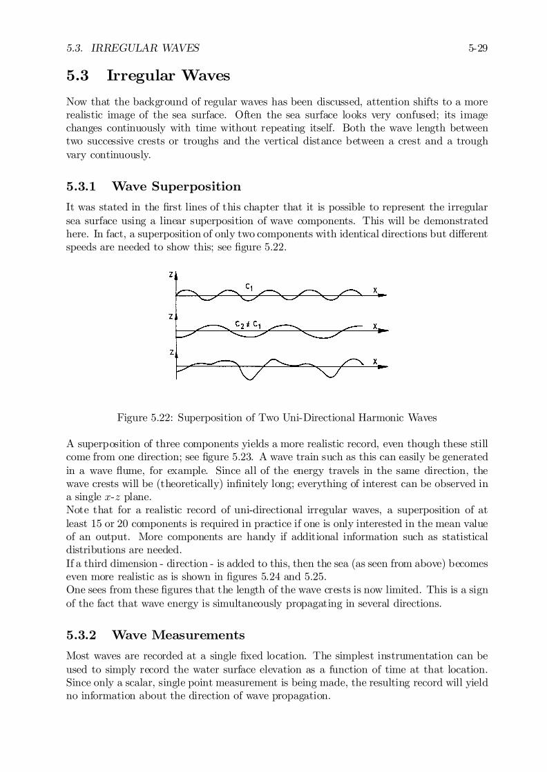
5.3. IRREGULAR WAVES 5-29
5.3 Irregular Waves
Now that the background of regular waves has been discussed, attention shifts to a morerealistic image of the sea surface. Often the sea surface looks very confused; its imagechanges continuously with time without repeating itself. Both the wave length betweentwo successive crests or troughs and the vertical distance between a crest and a troughvary continuously.
5.3.1 Wave Superposition
It was stated in the …rst lines of this chapter that it is possible to represent the irregularsea surface using a linear superposition of wave components. This will be demonstratedhere. In fact, a superposition of only two components with identical directions but di¤erentspeeds are needed to show this; see …gure 5.22.
Figure 5.22: Superposition of Two Uni-Directional Harmonic Waves
A superposition of three components yields a more realistic record, even though these stillcome from one direction; see …gure 5.23. A wave train such as this can easily be generatedin a wave ‡ume, for example. Since all of the energy travels in the same direction, thewave crests will be (theoretically) in…nitely long; everything of interest can be observed ina single x-z plane.Note that for a realistic record of uni-directional irregular waves, a superposition of atleast 15 or 20 components is required in practice if one is only interested in the mean valueof an output. More components are handy if additional information such as statisticaldistributions are needed.If a third dimension - direction - is added to this, then the sea (as seen from above) becomeseven more realistic as is shown in …gures 5.24 and 5.25.One sees from these …gures that the length of the wave crests is now limited. This is a signof the fact that wave energy is simultaneously propagating in several directions.
5.3.2 Wave Measurements
Most waves are recorded at a single …xed location. The simplest instrumentation can beused to simply record the water surface elevation as a function of time at that location.Since only a scalar, single point measurement is being made, the resulting record will yieldno information about the direction of wave propagation.

5-30 CHAPTER 5. OCEAN SURFACE WAVES
Figure 5.23: Superposition of Three Uni-Directional Harmonic Waves
Figure 5.24: Superposition of Two Harmonic Waves with Di¤erent Directions
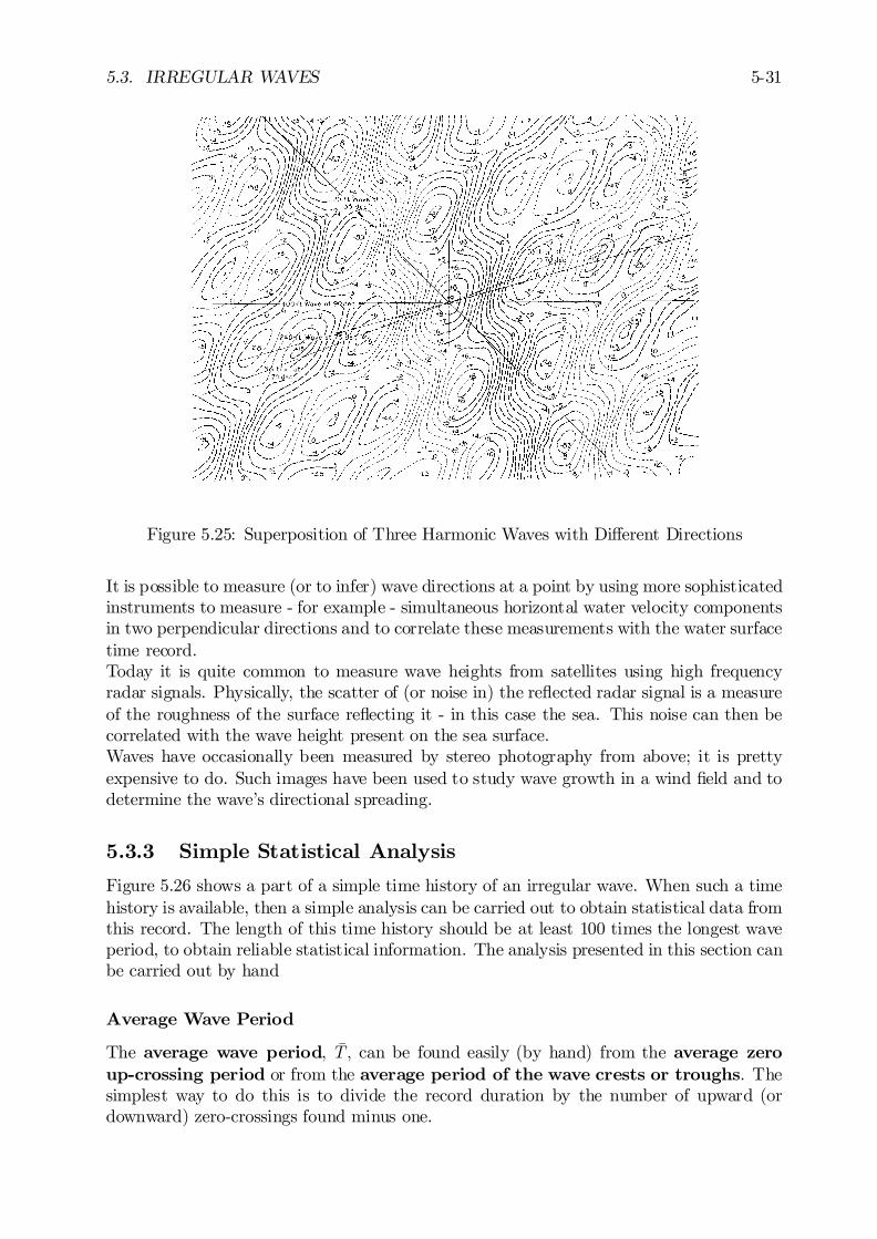
5.3. IRREGULAR WAVES 5-31
Figure 5.25: Superposition of Three Harmonic Waves with Di¤erent Directions
It is possible to measure (or to infer) wave directions at a point by using more sophisticatedinstruments to measure - for example - simultaneous horizontal water velocity componentsin two perpendicular directions and to correlate these measurements with the water surfacetime record.Today it is quite common to measure wave heights from satellites using high frequencyradar signals. Physically, the scatter of (or noise in) the re‡ected radar signal is a measureof the roughness of the surface re‡ecting it - in this case the sea. This noise can then becorrelated with the wave height present on the sea surface.Waves have occasionally been measured by stereo photography from above; it is prettyexpensive to do. Such images have been used to study wave growth in a wind …eld and todetermine the wave’s directional spreading.
5.3.3 Simple Statistical Analysis
Figure 5.26 shows a part of a simple time history of an irregular wave. When such a timehistory is available, then a simple analysis can be carried out to obtain statistical data fromthis record. The length of this time history should be at least 100 times the longest waveperiod, to obtain reliable statistical information. The analysis presented in this section canbe carried out by hand
Average Wave Period
The average wave period, ¹T; can be found easily (by hand) from the average zeroup-crossing period or from the average period of the wave crests or troughs. Thesimplest way to do this is to divide the record duration by the number of upward (ordownward) zero-crossings found minus one.
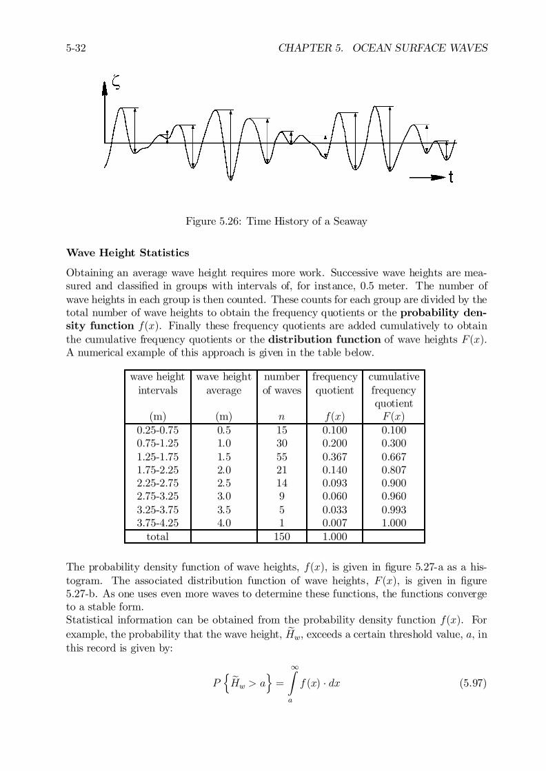
5-32 CHAPTER 5. OCEAN SURFACE WAVES
Figure 5.26: Time History of a Seaway
Wave Height Statistics
Obtaining an average wave height requires more work. Successive wave heights are mea-sured and classi…ed in groups with intervals of, for instance, 0.5 meter. The number ofwave heights in each group is then counted. These counts for each group are divided by thetotal number of wave heights to obtain the frequency quotients or the probability den-sity function f(x). Finally these frequency quotients are added cumulatively to obtainthe cumulative frequency quotients or the distribution function of wave heights F (x).A numerical example of this approach is given in the table below.
wave height wave height number frequency cumulativeintervals average of waves quotient frequency
quotient(m) (m) n f(x) F (x)
0.25-0.75 0.5 15 0.100 0.1000.75-1.25 1.0 30 0.200 0.3001.25-1.75 1.5 55 0.367 0.6671.75-2.25 2.0 21 0.140 0.8072.25-2.75 2.5 14 0.093 0.9002.75-3.25 3.0 9 0.060 0.9603.25-3.75 3.5 5 0.033 0.9933.75-4.25 4.0 1 0.007 1.000
total 150 1.000
The probability density function of wave heights, f(x), is given in …gure 5.27-a as a his-togram. The associated distribution function of wave heights, F (x), is given in …gure5.27-b. As one uses even more waves to determine these functions, the functions convergeto a stable form.Statistical information can be obtained from the probability density function f(x). Forexample, the probability that the wave height, eHw, exceeds a certain threshold value, a, inthis record is given by:
Pn
eHw > ao=
1Z
a
f (x) ¢ dx (5.97)
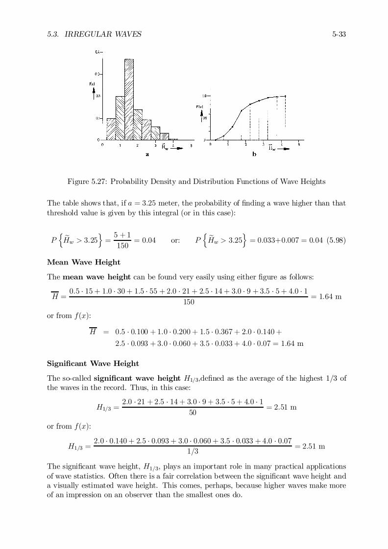
5.3. IRREGULAR WAVES 5-33
Figure 5.27: Probability Density and Distribution Functions of Wave Heights
The table shows that, if a = 3:25 meter, the probability of …nding a wave higher than thatthreshold value is given by this integral (or in this case):
Pn
eHw > 3:25o=5 +1
150= 0:04 or: P
neHw > 3:25
o= 0:033+0:007 = 0:04 (5.98)
Mean Wave Height
The mean wave height can be found very easily using either …gure as follows:
H =0:5 ¢ 15 + 1:0 ¢ 30 + 1:5 ¢ 55 + 2:0 ¢ 21 + 2:5 ¢ 14 + 3:0 ¢ 9 + 3:5 ¢ 5 + 4:0 ¢ 1
150= 1:64 m
or from f(x):
H = 0:5 ¢ 0:100 + 1:0 ¢ 0:200 + 1:5 ¢ 0:367 + 2:0 ¢ 0:140 +2:5 ¢ 0:093 + 3:0 ¢ 0:060 + 3:5 ¢ 0:033 + 4:0 ¢ 0:07 = 1:64 m
Signi…cant Wave Height
The so-called signi…cant wave height H1=3;de…ned as the average of the highest 1/3 ofthe waves in the record. Thus, in this case:
H1=3 =2:0 ¢ 21 + 2:5 ¢ 14 + 3:0 ¢ 9 + 3:5 ¢ 5 + 4:0 ¢ 1
50= 2:51 m
or from f(x):
H1=3 =2:0 ¢ 0:140 + 2:5 ¢ 0:093 + 3:0 ¢ 0:060 + 3:5 ¢ 0:033 + 4:0 ¢ 0:07
1=3= 2:51 m
The signi…cant wave height, H1=3, plays an important role in many practical applicationsof wave statistics. Often there is a fair correlation between the signi…cant wave height anda visually estimated wave height. This comes, perhaps, because higher waves make moreof an impression on an observer than the smallest ones do.
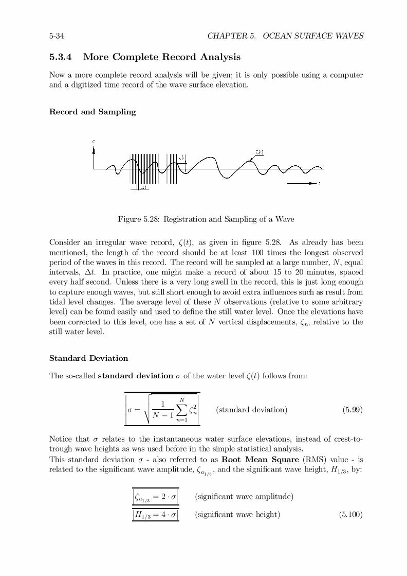
5-34 CHAPTER 5. OCEAN SURFACE WAVES
5.3.4 More Complete Record Analysis
Now a more complete record analysis will be given; it is only possible using a computerand a digitized time record of the wave surface elevation.
Record and Sampling
Figure 5.28: Registration and Sampling of a Wave
Consider an irregular wave record, ³(t), as given in …gure 5.28. As already has beenmentioned, the length of the record should be at least 100 times the longest observedperiod of the waves in this record. The record will be sampled at a large number, N , equalintervals, ¢t. In practice, one might make a record of about 15 to 20 minutes, spacedevery half second. Unless there is a very long swell in the record, this is just long enoughto capture enough waves, but still short enough to avoid extra in‡uences such as result fromtidal level changes. The average level of these N observations (relative to some arbitrarylevel) can be found easily and used to de…ne the still water level. Once the elevations havebeen corrected to this level, one has a set of N vertical displacements, ³n; relative to thestill water level.
Standard Deviation
The so-called standard deviation ¾ of the water level ³(t) follows from:
¯¯¯¾ =
vuut 1
N ¡ 1
NX
n=1
³2n
¯¯¯ (standard deviation) (5.99)
Notice that ¾ relates to the instantaneous water surface elevations, instead of crest-to-trough wave heights as was used before in the simple statistical analysis.This standard deviation ¾ - also referred to as Root Mean Square (RMS) value - isrelated to the signi…cant wave amplitude, ³a1=3 , and the signi…cant wave height, H1=3, by:
¯¯³a1=3 = 2 ¢ ¾
¯¯ (signi…cant wave amplitude)
¯H1=3 = 4 ¢ ¾
¯(signi…cant wave height) (5.100)
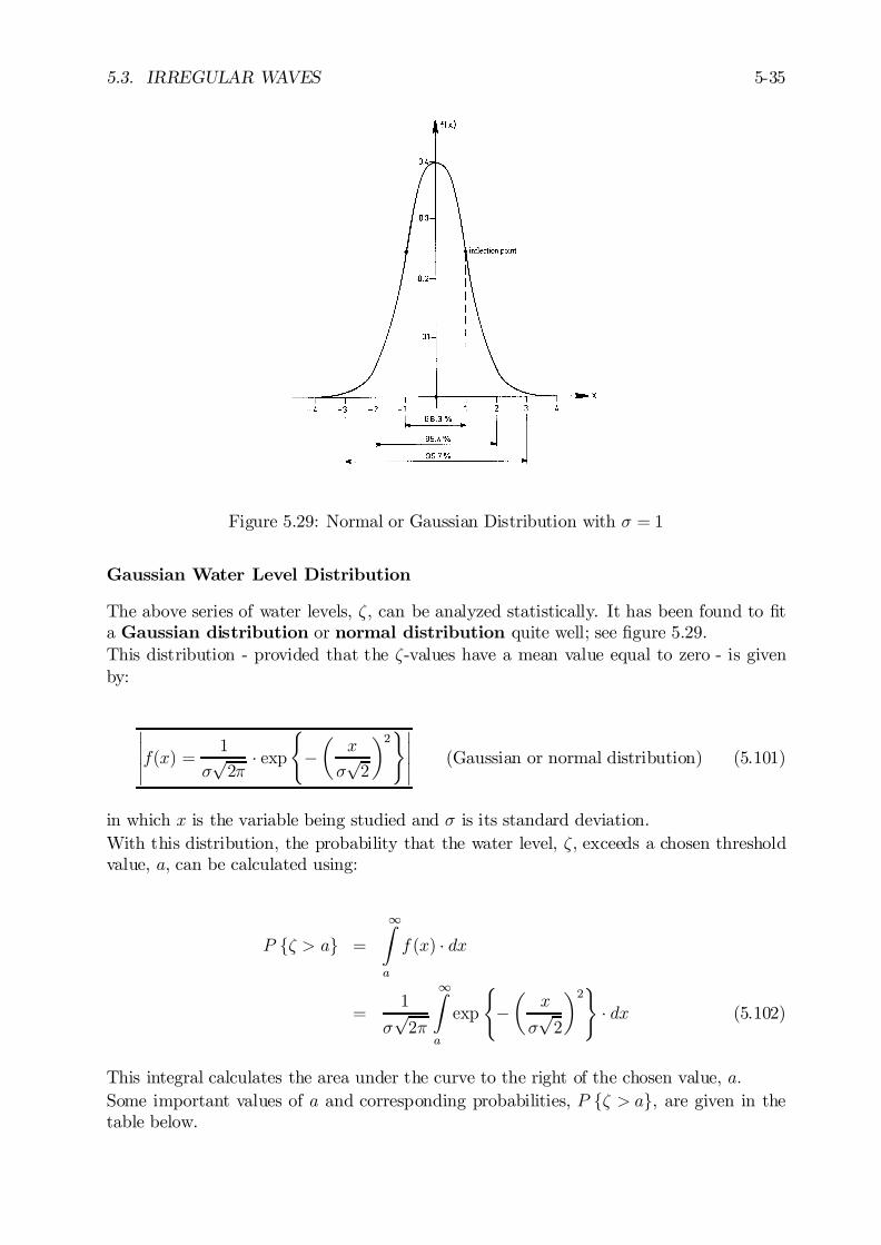
5.3. IRREGULAR WAVES 5-35
Figure 5.29: Normal or Gaussian Distribution with ¾ = 1
Gaussian Water Level Distribution
The above series of water levels, ³, can be analyzed statistically. It has been found to …ta Gaussian distribution or normal distribution quite well; see …gure 5.29.This distribution - provided that the ³-values have a mean value equal to zero - is givenby:
¯¯¯f(x) =
1
¾p2¼
¢ exp(
¡µx
¾p2
¶2)¯¯¯ (Gaussian or normal distribution) (5.101)
in which x is the variable being studied and ¾ is its standard deviation.With this distribution, the probability that the water level, ³, exceeds a chosen thresholdvalue, a, can be calculated using:
P f³ > ag =
1Z
a
f (x) ¢ dx
=1
¾p2¼
1Z
a
exp
(¡
µx
¾p2
¶2)
¢ dx (5.102)
This integral calculates the area under the curve to the right of the chosen value, a:Some important values of a and corresponding probabilities, P f³ > ag, are given in thetable below.

5-36 CHAPTER 5. OCEAN SURFACE WAVES
a P f³ > ag¾ 0.3202¾ 0.0463¾ 0.003
A Gaussian or normal distribution with ¾ = 1 is shown in …gure 5.29. This distribution hasits in‡ection points at x = §¾ = §1 and its value at x = 0 is f (0) = 1=(¾
p2¼) = 0:399.
Rayleigh Wave Amplitude Distribution
If the range of frequencies in a wave …eld is not too large, one speaks of a narrow bandedfrequency spectrum. Luckily, waves - a sea or a swell - generally satisfy this conditionquite well. If this is the case - and the water surface elevation is a Gaussian distribution -then the wave amplitude statistics will obey a Rayleigh distribution.This Rayleigh distribution is given by:
¯¯¯f(x) =
x
¾2¢ exp
(¡
µx
¾p2
¶2)¯
¯¯ (Rayleigh distribution) (5.103)
in which x is the variable being studied and ¾ is its standard deviation.With this Rayleigh distribution, the probability that the wave amplitude, ³a, exceeds achosen threshold value, a, can be calculated using:
P f³a > ag =
1Z
a
f(x) ¢ dx
=1
¾2
1Z
a
x ¢ exp(
¡µx
¾p2
¶2)
¢ dx
= exp
½¡ a2
2¾2
¾(5.104)
These probabilities for wave crest elevations can also be expressed in terms of the crest-to-trough wave heights Hw:
¯¯¯P fHw > Hg = exp
(¡2
µH
H1=3
¶2)¯
¯¯ (5.105)
in which P fHw > Hg is the chance that any individual wave height H is exceeded in awave …eld characterized by a signi…cant wave height, H1=3 = 4¾.The Rayleigh probability density function is illustrated in …gure 5.30-a; …gure 5.30-b showsthe probability of exceeding in percentages, P (H), in relation to the wave height ratio,H=H1=3, on a logarithmic scale. Notice that all values in …gures 5.30-a and 5.30-b arenow positive. Indeed, if one chooses H = 0 in equation 5.105, then one …nds that theprobability that it is exceeded is exactly 1.
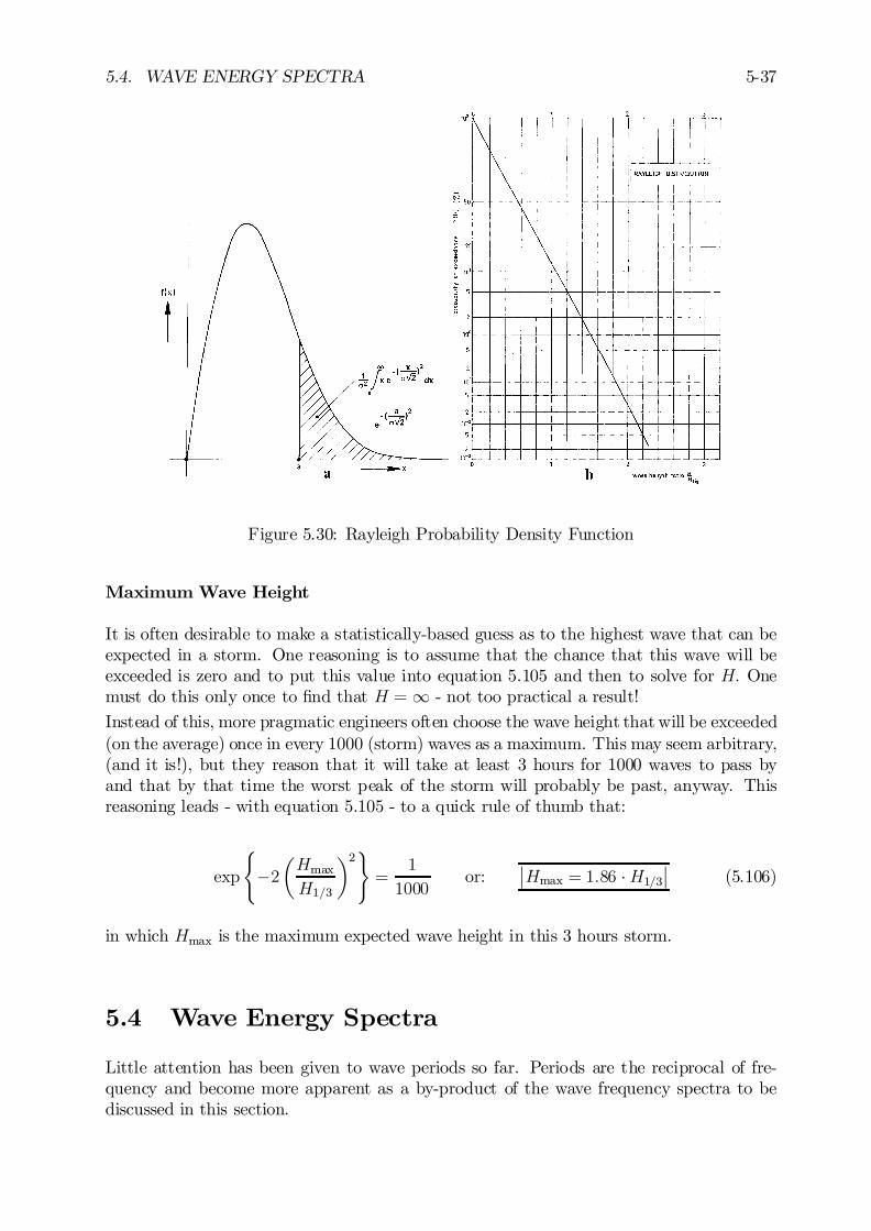
5.4. WAVE ENERGY SPECTRA 5-37
Figure 5.30: Rayleigh Probability Density Function
Maximum Wave Height
It is often desirable to make a statistically-based guess as to the highest wave that can beexpected in a storm. One reasoning is to assume that the chance that this wave will beexceeded is zero and to put this value into equation 5.105 and then to solve for H: Onemust do this only once to …nd that H = 1 - not too practical a result!
Instead of this, more pragmatic engineers often choose the wave height that will be exceeded(on the average) once in every 1000 (storm) waves as a maximum. This may seem arbitrary,(and it is!), but they reason that it will take at least 3 hours for 1000 waves to pass byand that by that time the worst peak of the storm will probably be past, anyway. Thisreasoning leads - with equation 5.105 - to a quick rule of thumb that:
exp
(¡2
µHmaxH1=3
¶2)=
1
1000or:
¯Hmax = 1:86 ¢H1=3
¯(5.106)
in which Hmax is the maximum expected wave height in this 3 hours storm.
5.4 Wave Energy Spectra
Little attention has been given to wave periods so far. Periods are the reciprocal of fre-quency and become more apparent as a by-product of the wave frequency spectra to bediscussed in this section.
5-38 CHAPTER 5. OCEAN SURFACE WAVES
5.4.1 Basic Principles
Since an irregular wave can be seen as the superposition of a series of sinusoidal waves,it is only logical to study the frequency characteristics of such an irregular signal usingFourier series analysis. To do this, one selects a time record segment containing manywaves. Indeed, one assumption implicit in this analysis - see appendix C - is that thesignal being studied repeats itself after each (long) interval. A wave record does not dothis exactly, but that little detail is neglected in this case.The wave elevation (in the time domain) of a long-crested irregular sea, propagating alongthe positive x axis, can be written as the sum of a large number of regular wave components(in the frequency domain):
¯¯¯³(t) =
NX
n=1
³an cos(knx¡ !nt+ "n)¯¯¯ (5.107)
in which, for each component, n:
³an = wave amplitude component (m)!n = circular frequency component (rad/s)kn = wave number component (rad/m)"n = random phase angle component (rad)
A Fourier series analysis carried out at one location would not indicate anything about k;this is location-dependent. This is not a problem in our case, since kn and !n are relatedby the known dispersion relation already given earlier in this chapter.The Fourier series will thus yield a set of values for ³an and "n , each associated with itsown !n: If enough Fourier series terms are included, the entire time record at that pointcan be reproduced using this set of values. In practice, however, one is not really interestedin the exact water level at some time t (which is already history!). It is su¢cient to knowonly the statistical properties - now in terms of both frequency and amplitude - of thesignal. This means that the "n can be discarded.
5.4.2 Energy Density Spectrum
Suppose a time history, as given in …gure 5.28, of the wave elevation during a su¢cientlong but arbitrary period:
¿ = N ¢¢t
The instantaneous wave elevation is supposed to has a Gaussian distribution and zeromean.The amplitudes ³an can be obtained by a Fourier analysis of the signal. However, for eachlittle time shift of the time history one will …nd a new series of amplitudes ³an. Luckily, a
mean square value of ³an can be found: ³2an .
When ³(t) is an irregular signal without prevailing frequencies, the average values ³2an close
to !n will not change much as a function of the frequency; ³2a is a continuous function.
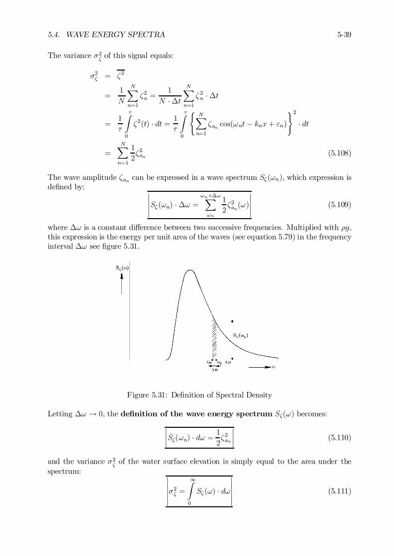
5.4. WAVE ENERGY SPECTRA 5-39
The variance ¾2³ of this signal equals:
¾2³ = ³2
=1
N
NX
n=1
³2n =1
N ¢¢t
NX
n=1
³ 2n ¢¢t
=1
¿
¿Z
0
³2(t) ¢ dt = 1
¿
¿Z
0
(NX
n=1
³an cos(!nt¡ knx+ "n))2
¢ dt
=NX
n=1
1
2³2an (5.108)
The wave amplitude ³an can be expressed in a wave spectrum S³ (!n), which expression isde…ned by: ¯
¯¯S³ (!n) ¢¢! =
!n+¢!X
!n
1
2³2an(!)
¯¯¯ (5.109)
where ¢! is a constant di¤erence between two successive frequencies. Multiplied with ½g,this expression is the energy per unit area of the waves (see equation 5.79) in the frequencyinterval ¢! see …gure 5.31.
Figure 5.31: De…nition of Spectral Density
Letting ¢! ! 0, the de…nition of the wave energy spectrum S³(!) becomes:
¯¯S³(!n) ¢ d! = 1
2³2an
¯¯ (5.110)
and the variance ¾2³ of the water surface elevation is simply equal to the area under thespectrum: ¯
¯¯¾2³ =
1Z
0
S³ (!) ¢ d!
¯¯¯ (5.111)
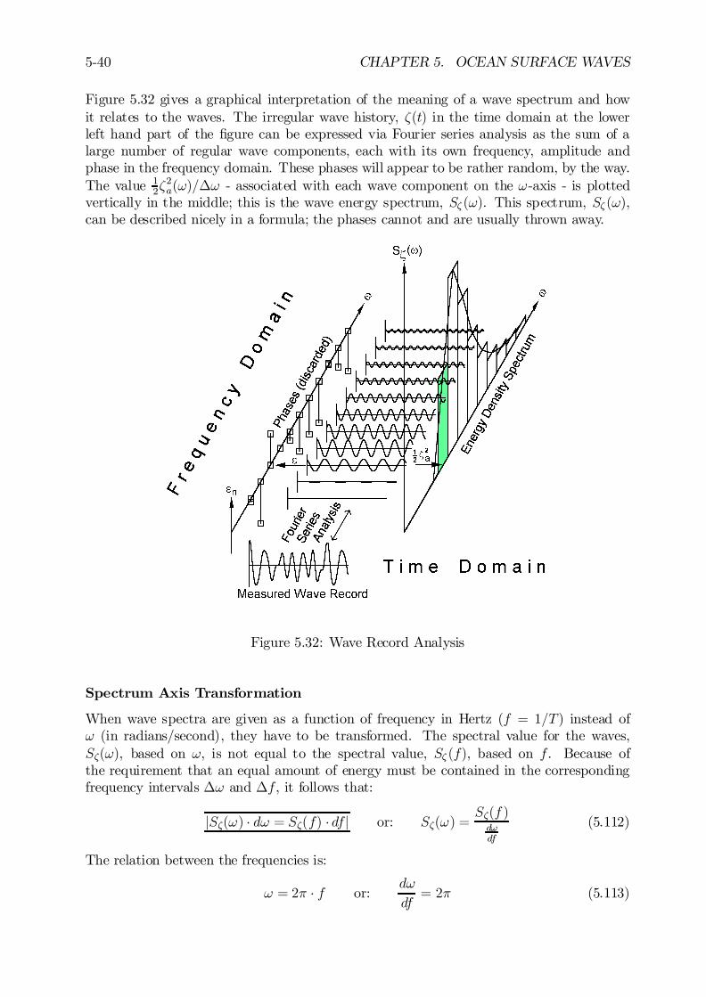
5-40 CHAPTER 5. OCEAN SURFACE WAVES
Figure 5.32 gives a graphical interpretation of the meaning of a wave spectrum and howit relates to the waves. The irregular wave history, ³(t) in the time domain at the lowerleft hand part of the …gure can be expressed via Fourier series analysis as the sum of alarge number of regular wave components, each with its own frequency, amplitude andphase in the frequency domain. These phases will appear to be rather random, by the way.The value 1
2³2a(!)=¢! - associated with each wave component on the !-axis - is plotted
vertically in the middle; this is the wave energy spectrum, S³ (!). This spectrum, S³ (!),can be described nicely in a formula; the phases cannot and are usually thrown away.
Figure 5.32: Wave Record Analysis
Spectrum Axis Transformation
When wave spectra are given as a function of frequency in Hertz (f = 1=T) instead of! (in radians/second), they have to be transformed. The spectral value for the waves,S³(!), based on !, is not equal to the spectral value, S³ (f), based on f. Because ofthe requirement that an equal amount of energy must be contained in the correspondingfrequency intervals ¢! and ¢f, it follows that:
jS³(!) ¢ d! = S³(f) ¢ dfj or: S³(!) =S³(f )d!df
(5.112)
The relation between the frequencies is:
! = 2¼ ¢ f or:d!
df= 2¼ (5.113)
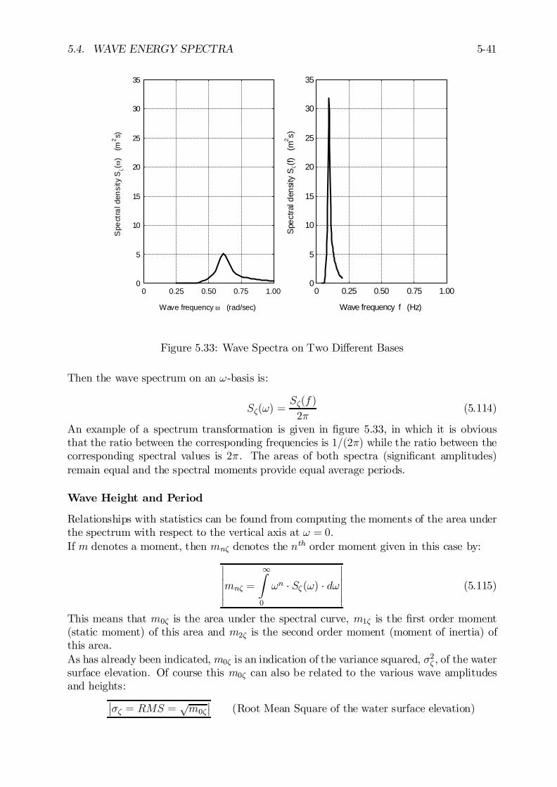
5.4. WAVE ENERGY SPECTRA 5-41
0
5
10
15
20
25
30
35
0 0.25 0.50 0.75 1.00
Wave frequency f (Hz)
Spe
ctra
l den
sity
Sζ(
f) (
m2 s)
0
5
10
15
20
25
30
35
0 0.25 0.50 0.75 1.00
Wave frequency ω (rad/sec)
Spe
ctra
l den
sity
Sζ(
ω)
(m
2 s)
Figure 5.33: Wave Spectra on Two Di¤erent Bases
Then the wave spectrum on an !-basis is:
S³(!) =S³(f )
2¼(5.114)
An example of a spectrum transformation is given in …gure 5.33, in which it is obviousthat the ratio between the corresponding frequencies is 1=(2¼) while the ratio between thecorresponding spectral values is 2¼. The areas of both spectra (signi…cant amplitudes)remain equal and the spectral moments provide equal average periods.
Wave Height and Period
Relationships with statistics can be found from computing the moments of the area underthe spectrum with respect to the vertical axis at ! = 0.If m denotes a moment, then mn³ denotes the nth order moment given in this case by:
¯¯¯mn³ =
1Z
0
!n ¢ S³ (!) ¢ d!
¯¯¯ (5.115)
This means that m0³ is the area under the spectral curve, m1³ is the …rst order moment(static moment) of this area and m2³ is the second order moment (moment of inertia) ofthis area.As has already been indicated, m0³ is an indication of the variance squared, ¾2³ , of the watersurface elevation. Of course this m0³ can also be related to the various wave amplitudesand heights:
¯¾³ = RMS =
pm0³
¯(Root Mean Square of the water surface elevation)
5-42 CHAPTER 5. OCEAN SURFACE WAVES
¯¯³a1=3 = 2 ¢ p
m0³¯¯ (signi…cant wave amplitude)
¯H1=3 = 4 ¢ p
m0³
¯(signi…cant wave height) (5.116)
Characteristic wave periods can be de…ned from the spectral moments:
m1³ = !1 ¢m0³ with !1 is spectral centroid
m2³ = !22 ¢m0³ with !2 is spectral radius of inertia (5.117)
as follows:
¯¯T1 = 2¼ ¢ m0³
m1³
¯¯ (mean centroid wave period)
¯¯T2 = 2¼ ¢
rm0³
m2³
¯¯ (mean zero-crossing wave period) (5.118)
The mean zero-crossing period, T2, is sometimes indicated by Tz. One will often …nd theperiod associated with the peak of the spectrum, Tp, in the literature as well.
Rayleigh Distribution
Expressed in terms of m0x, the Rayleigh distribution of amplitudes xa is given by:
¯¯f (x) = x
m0x
¢ exp½
¡ x2
2 ¢m0x
¾¯¯ (Rayleigh distribution) (5.119)
in which x is the variable being studied and m0x is the area under the spectral curve.With this distribution, the probability that the amplitude, xa, exceeds a chosen thresholdvalue, a, can be calculated using:
P fxa > ag =
1Z
a
f (x) ¢ dx
=1
m0x
1Z
a
x ¢ exp½
¡ x2
2 ¢m0x
¾¢ dx
= exp
½¡ a2
2 ¢m0x
¾(5.120)
It is obvious here that expf¡ug means e¡u.As an example for waves, the probability that the wave height, Hw, in a certain sea stateexceeds the signi…cant wave height, H1=3, is found by:
P©Hw > H1=3
ª= P
n³a > ³ a1=3
o
= exp
(¡³2a1=32 ¢m0³
)
= e¡2 t 0:135 t 1
7(5.121)
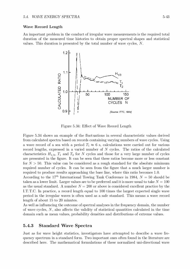
5.4. WAVE ENERGY SPECTRA 5-43
Wave Record Length
An important problem in the conduct of irregular wave measurements is the required totalduration of the measured time histories to obtain proper spectral shapes and statisticalvalues. This duration is presented by the total number of wave cycles, N .
Figure 5.34: E¤ect of Wave Record Length
Figure 5.34 shows an example of the ‡uctuations in several characteristic values derivedfrom calculated spectra based on records containing varying numbers of wave cycles. Usinga wave record of a sea with a period T1 t 6 s, calculations were carried out for variousrecord lengths, expressed in a varied number of N cycles. The ratios of the calculatedcharacteristics H1=3, T1 and T2 for N cycles and those for a very large number of cyclesare presented in the …gure. It can be seen that these ratios become more or less constantfor N > 50. This value can be considered as a rough standard for the absolute minimumrequired number of cycles. It can be seen from the …gure that a much larger number isrequired to produce results approaching the base line, where this ratio becomes 1.0.According to the 17th International Towing Tank Conference in 1984, N = 50 should betaken as a lower limit. Larger values are to be preferred and it is more usual to take N = 100as the usual standard. A number N = 200 or above is considered excellent practice by theI.T.T.C. In practice, a record length equal to 100 times the largest expected single waveperiod in the irregular waves is often used as a safe standard. This means a wave recordlength of about 15 to 20 minutes.As well as in‡uencing the outcome of spectral analyses in the frequency domain, the numberof wave cycles, N , also a¤ects the validity of statistical quantities calculated in the timedomain such as mean values, probability densities and distributions of extreme values.
5.4.3 Standard Wave Spectra
Just as for wave height statistics, investigators have attempted to describe a wave fre-quency spectrum in a standard form. Two important ones often found in the literature aredescribed here. The mathematical formulations of these normalized uni-directional wave
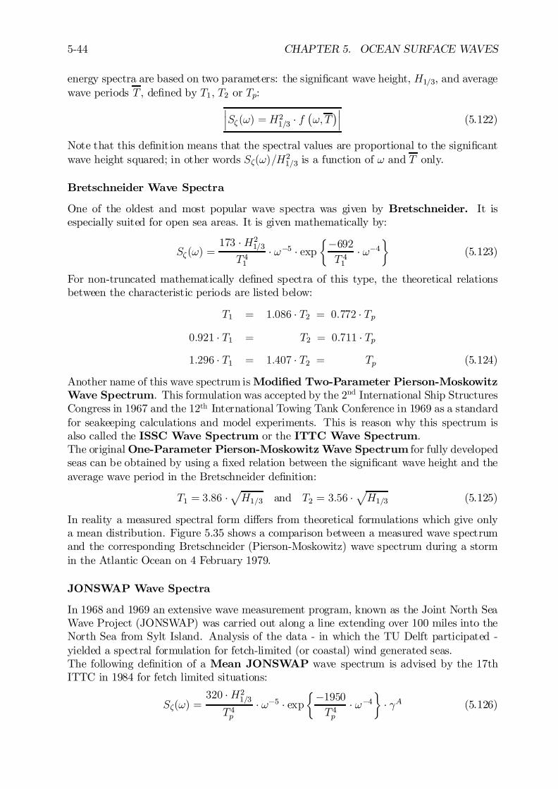
5-44 CHAPTER 5. OCEAN SURFACE WAVES
energy spectra are based on two parameters: the signi…cant wave height, H1=3, and averagewave periods T , de…ned by T1, T2 or Tp:
¯¯S³ (!) =H2
1=3 ¢ f¡!; T
¢¯¯ (5.122)
Note that this de…nition means that the spectral values are proportional to the signi…cantwave height squared; in other words S³(!)=H2
1=3 is a function of ! and T only.
Bretschneider Wave Spectra
One of the oldest and most popular wave spectra was given by Bretschneider. It isespecially suited for open sea areas. It is given mathematically by:
S³ (!) =173 ¢H2
1=3
T 41¢ !¡5 ¢ exp
½¡692T 41
¢ !¡4¾
(5.123)
For non-truncated mathematically de…ned spectra of this type, the theoretical relationsbetween the characteristic periods are listed below:
T1 = 1:086 ¢ T2 = 0:772 ¢ Tp
0:921 ¢ T1 = T2 = 0:711 ¢ Tp1:296 ¢ T1 = 1:407 ¢ T2 = Tp (5.124)
Another name of this wave spectrum is Modi…ed Two-Parameter Pierson-MoskowitzWave Spectrum. This formulation was accepted by the 2nd International Ship StructuresCongress in 1967 and the 12th International Towing Tank Conference in 1969 as a standardfor seakeeping calculations and model experiments. This is reason why this spectrum isalso called the ISSC Wave Spectrum or the ITTC Wave Spectrum.The original One-Parameter Pierson-Moskowitz Wave Spectrum for fully developedseas can be obtained by using a …xed relation between the signi…cant wave height and theaverage wave period in the Bretschneider de…nition:
T1 = 3:86 ¢pH1=3 and T2 = 3:56 ¢
pH1=3 (5.125)
In reality a measured spectral form di¤ers from theoretical formulations which give onlya mean distribution. Figure 5.35 shows a comparison between a measured wave spectrumand the corresponding Bretschneider (Pierson-Moskowitz) wave spectrum during a stormin the Atlantic Ocean on 4 February 1979.
JONSWAP Wave Spectra
In 1968 and 1969 an extensive wave measurement program, known as the Joint North SeaWave Project (JONSWAP) was carried out along a line extending over 100 miles into theNorth Sea from Sylt Island. Analysis of the data - in which the TU Delft participated -yielded a spectral formulation for fetch-limited (or coastal) wind generated seas.The following de…nition of a Mean JONSWAP wave spectrum is advised by the 17thITTC in 1984 for fetch limited situations:
S³(!) =320 ¢H2
1=3
T 4p¢ !¡5 ¢ exp
½¡1950T 4p
¢ !¡4¾
¢ °A (5.126)
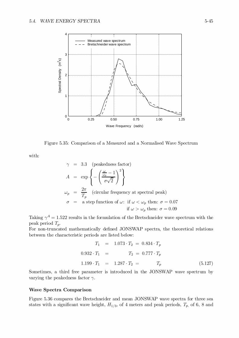
5.4. WAVE ENERGY SPECTRA 5-45
0
1
2
3
4
0 0.25 0.50 0.75 1.00 1.25
Measured wave spectrumBretschneider wave spectrum
Wave Frequency (rad/s)
Spe
ctra
l Den
sity
(m
2 s)
Figure 5.35: Comparison of a Measured and a Normalised Wave Spectrum
with:
° = 3:3 (peakedness factor)
A = exp
8<:¡
Ã!!p
¡ 1¾p2
!29=;
!p =2¼
Tp(circular frequency at spectral peak)
¾ = a step function of !: if ! < !p then: ¾ = 0:07
if ! > !p then: ¾ = 0:09
Taking °A = 1.522 results in the formulation of the Bretschneider wave spectrum with thepeak period Tp.For non-truncated mathematically de…ned JONSWAP spectra, the theoretical relationsbetween the characteristic periods are listed below:
T1 = 1:073 ¢ T2 = 0:834 ¢ Tp0:932 ¢ T1 = T2 = 0:777 ¢ Tp
1:199 ¢ T1 = 1:287 ¢ T2 = Tp (5.127)
Sometimes, a third free parameter is introduced in the JONSWAP wave spectrum byvarying the peakedness factor °.
Wave Spectra Comparison
Figure 5.36 compares the Bretschneider and mean JONSWAP wave spectra for three seastates with a signi…cant wave height, H1=3, of 4 meters and peak periods, Tp, of 6, 8 and
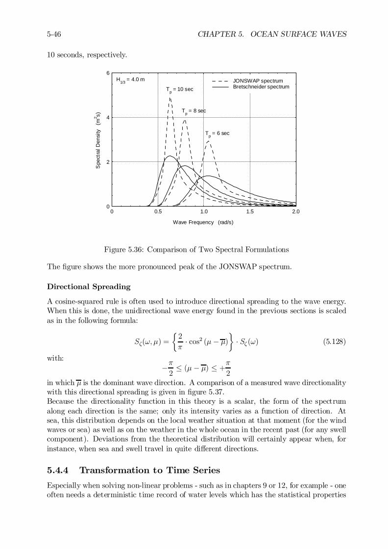
5-46 CHAPTER 5. OCEAN SURFACE WAVES
10 seconds, respectively.
0
2
4
6
0 0.5 1.0 1.5 2.0
JONSWAP spectrumBretschneider spectrum
H1/3 = 4.0 m
Tp = 10 sec
Tp = 8 sec
Tp = 6 sec
Wave Frequency (rad/s)
Spe
ctra
l Den
sity
(m
2 s)
Figure 5.36: Comparison of Two Spectral Formulations
The …gure shows the more pronounced peak of the JONSWAP spectrum.
Directional Spreading
A cosine-squared rule is often used to introduce directional spreading to the wave energy.When this is done, the unidirectional wave energy found in the previous sections is scaledas in the following formula:
S³(!; ¹) =
½2
¼¢ cos2 (¹¡ ¹)
¾¢ S³ (!) (5.128)
with:¡¼2
· (¹¡ ¹) · +¼
2in which ¹ is the dominant wave direction. A comparison of a measured wave directionalitywith this directional spreading is given in …gure 5.37.Because the directionality function in this theory is a scalar, the form of the spectrumalong each direction is the same; only its intensity varies as a function of direction. Atsea, this distribution depends on the local weather situation at that moment (for the windwaves or sea) as well as on the weather in the whole ocean in the recent past (for any swellcomponent). Deviations from the theoretical distribution will certainly appear when, forinstance, when sea and swell travel in quite di¤erent directions.
5.4.4 Transformation to Time Series
Especially when solving non-linear problems - such as in chapters 9 or 12, for example - oneoften needs a deterministic time record of water levels which has the statistical properties
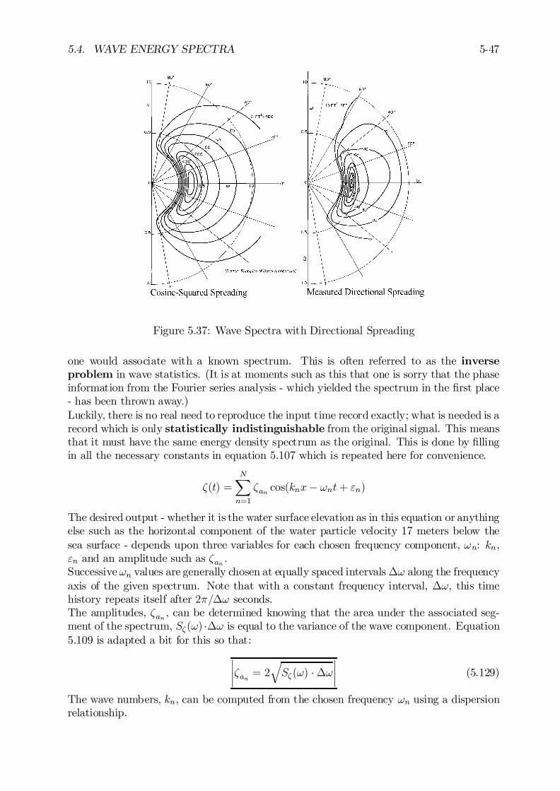
5.4. WAVE ENERGY SPECTRA 5-47
Figure 5.37: Wave Spectra with Directional Spreading
one would associate with a known spectrum. This is often referred to as the inverseproblem in wave statistics. (It is at moments such as this that one is sorry that the phaseinformation from the Fourier series analysis - which yielded the spectrum in the …rst place- has been thrown away.)Luckily, there is no real need to reproduce the input time record exactly; what is needed is arecord which is only statistically indistinguishable from the original signal. This meansthat it must have the same energy density spectrum as the original. This is done by …llingin all the necessary constants in equation 5.107 which is repeated here for convenience.
³(t) =NX
n=1
³an cos(knx¡ !nt+ "n)
The desired output - whether it is the water surface elevation as in this equation or anythingelse such as the horizontal component of the water particle velocity 17 meters below thesea surface - depends upon three variables for each chosen frequency component, !n: kn,"n and an amplitude such as ³an .Successive!n values are generally chosen at equally spaced intervals¢! along the frequencyaxis of the given spectrum. Note that with a constant frequency interval, ¢!, this timehistory repeats itself after 2¼=¢! seconds.The amplitudes, ³an , can be determined knowing that the area under the associated seg-ment of the spectrum, S³ (!) ¢¢! is equal to the variance of the wave component. Equation5.109 is adapted a bit for this so that:
¯¯³an = 2
qS³ (!) ¢¢!
¯¯ (5.129)
The wave numbers, kn, can be computed from the chosen frequency !n using a dispersionrelationship.
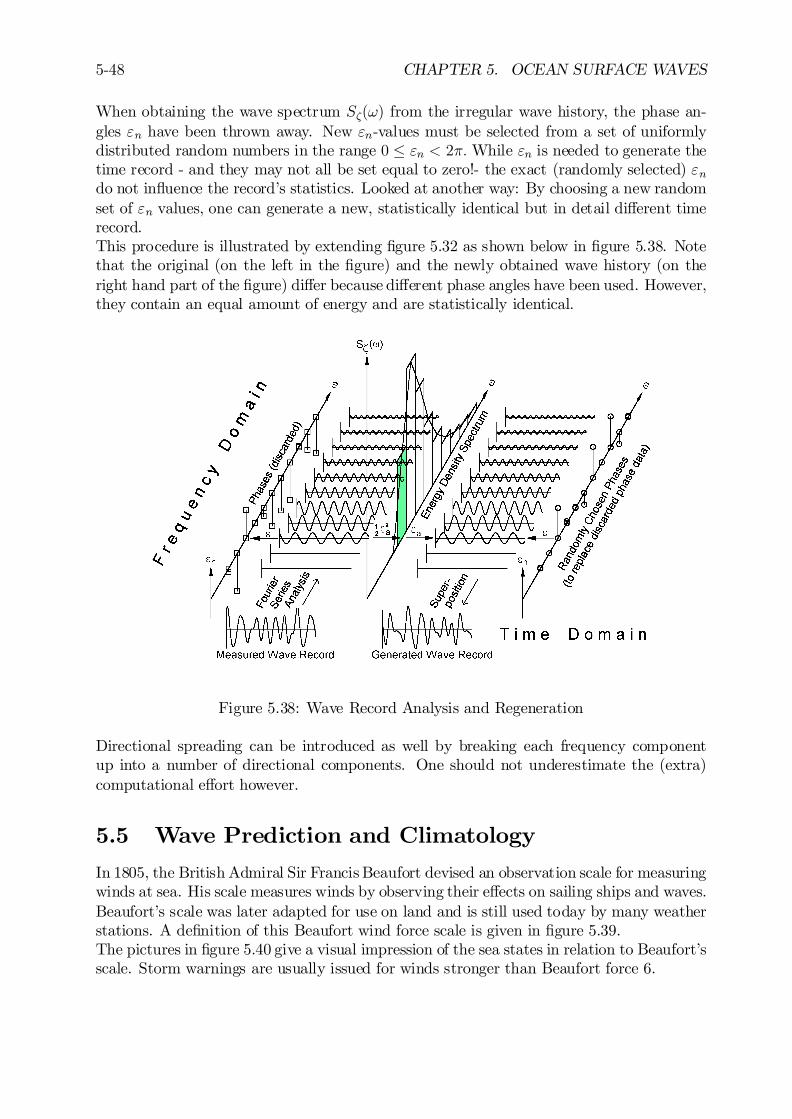
5-48 CHAPTER 5. OCEAN SURFACE WAVES
When obtaining the wave spectrum S³(!) from the irregular wave history, the phase an-gles "n have been thrown away. New "n-values must be selected from a set of uniformlydistributed random numbers in the range 0 · "n < 2¼: While "n is needed to generate thetime record - and they may not all be set equal to zero!- the exact (randomly selected) "ndo not in‡uence the record’s statistics. Looked at another way: By choosing a new randomset of "n values, one can generate a new, statistically identical but in detail di¤erent timerecord.This procedure is illustrated by extending …gure 5.32 as shown below in …gure 5.38. Notethat the original (on the left in the …gure) and the newly obtained wave history (on theright hand part of the …gure) di¤er because di¤erent phase angles have been used. However,they contain an equal amount of energy and are statistically identical.
Figure 5.38: Wave Record Analysis and Regeneration
Directional spreading can be introduced as well by breaking each frequency componentup into a number of directional components. One should not underestimate the (extra)computational e¤ort however.
5.5 Wave Prediction and Climatology
In 1805, the British Admiral Sir Francis Beaufort devised an observation scale for measuringwinds at sea. His scale measures winds by observing their e¤ects on sailing ships and waves.Beaufort’s scale was later adapted for use on land and is still used today by many weatherstations. A de…nition of this Beaufort wind force scale is given in …gure 5.39.The pictures in …gure 5.40 give a visual impression of the sea states in relation to Beaufort’sscale. Storm warnings are usually issued for winds stronger than Beaufort force 6.
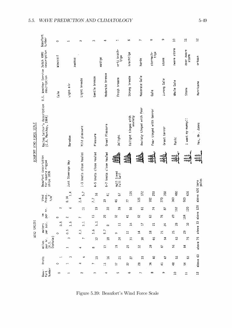
5.5. WAVE PREDICTION AND CLIMATOLOGY 5-49
Figure 5.39: Beaufort’s Wind Force Scale
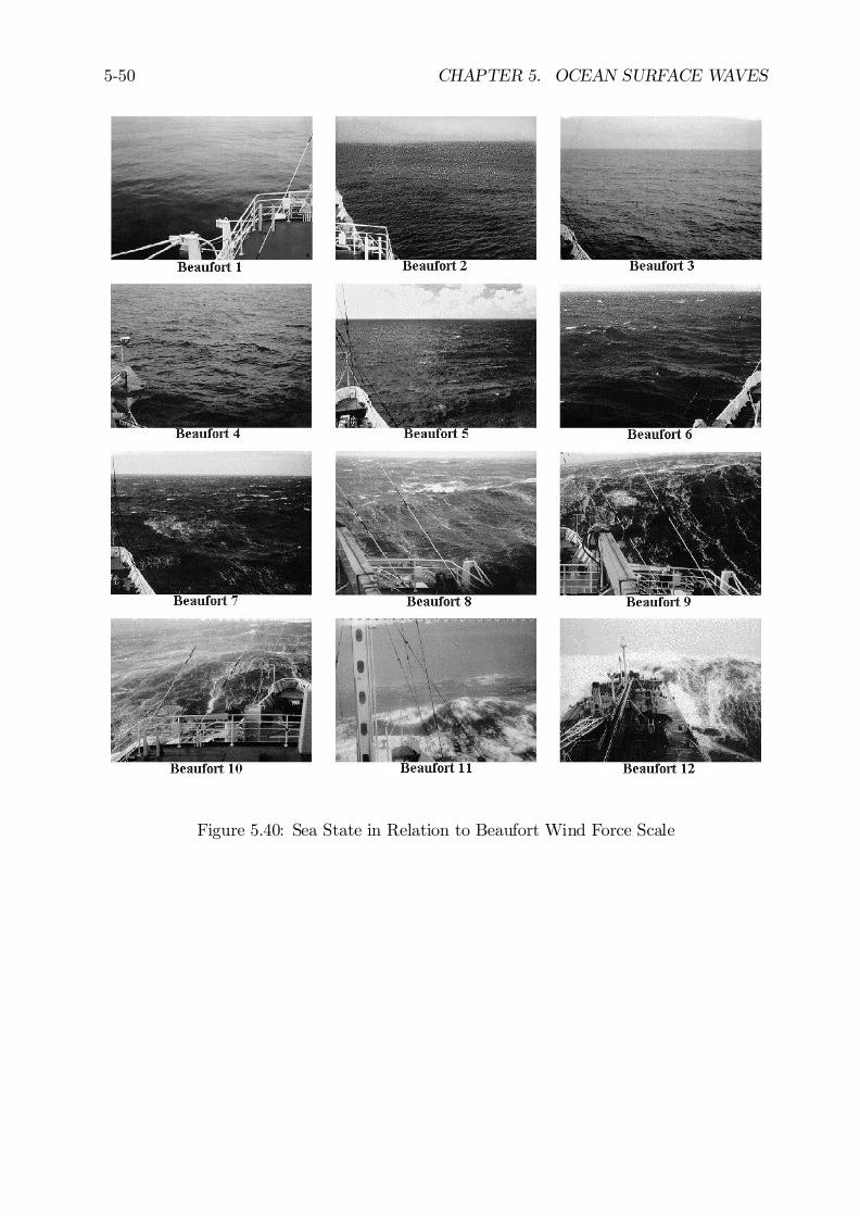
5-50 CHAPTER 5. OCEAN SURFACE WAVES
Figure 5.40: Sea State in Relation to Beaufort Wind Force Scale
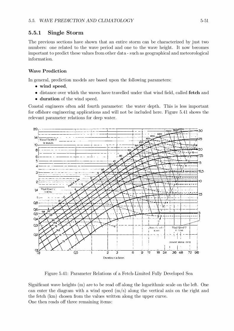
5.5. WAVE PREDICTION AND CLIMATOLOGY 5-51
5.5.1 Single Storm
The previous sections have shown that an entire storm can be characterized by just twonumbers: one related to the wave period and one to the wave height. It now becomesimportant to predict these values from other data - such as geographical and meteorologicalinformation.
Wave Prediction
In general, prediction models are based upon the following parameters:² wind speed,² distance over which the waves have travelled under that wind …eld, called fetch and² duration of the wind speed.
Coastal engineers often add fourth parameter: the water depth. This is less importantfor o¤shore engineering applications and will not be included here. Figure 5.41 shows therelevant parameter relations for deep water.
Figure 5.41: Parameter Relations of a Fetch-Limited Fully Developed Sea
Signi…cant wave heights (m) are to be read o¤ along the logarithmic scale on the left. Onecan enter the diagram with a wind speed (m/s) along the vertical axis on the right andthe fetch (km) chosen from the values written along the upper curve.One then reads o¤ three remaining items:
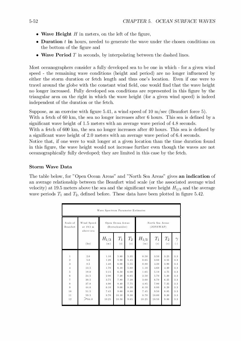
5-52 CHAPTER 5. OCEAN SURFACE WAVES
² Wave Height H in meters, on the left of the …gure,
² Duration t in hours, needed to generate the wave under the chosen conditions onthe bottom of the …gure and
² Wave Period T in seconds, by interpolating between the dashed lines.
Most oceanographers consider a fully developed sea to be one in which - for a given windspeed - the remaining wave conditions (height and period) are no longer in‡uenced byeither the storm duration or fetch length and thus one’s location. Even if one were totravel around the globe with the constant wind …eld, one would …nd that the wave heightno longer increased. Fully developed sea conditions are represented in this …gure by thetriangular area on the right in which the wave height (for a given wind speed) is indeedindependent of the duration or the fetch.
Suppose, as an exercise with …gure 5.41, a wind speed of 10 m/sec (Beaufort force 5).With a fetch of 60 km, the sea no longer increases after 6 hours. This sea is de…ned by asigni…cant wave height of 1.5 meters with an average wave period of 4.8 seconds.With a fetch of 600 km, the sea no longer increases after 40 hours. This sea is de…ned bya signi…cant wave height of 2.0 meters with an average wave period of 6.4 seconds.Notice that, if one were to wait longer at a given location than the time duration foundin this …gure, the wave height would not increase further even though the waves are notoceanographically fully developed; they are limited in this case by the fetch.
Storm Wave Data
The table below, for ”Open Ocean Areas” and ”North Sea Areas” gives an indication ofan average relationship between the Beaufort wind scale (or the associated average windvelocity) at 19.5 meters above the sea and the signi…cant wave height H1=3 and the averagewave periods T1 and T2, de…ned before. These data have been plotted in …gure 5.42.
Wave Sp ec tru m Param eter E st im ates
S ca le o f W ind Sp ee d Op en Oc ean A re as North Sea Areas
B eau fort at 19.5 m (B retsch neid er) (JONS WAP)
above se a
H1=3 T1 T2 H1=3 T1 T2 °(kn) (m ) (s) (s) (m ) (s) (s) ( -)
1 2 .0 1 .10 5 .80 5 .35 0 .50 3.50 3 .25 3 .3
2 5 .0 1 .20 5 .90 5 .45 0 .65 3.80 3 .55 3 .3
3 8 .5 1 .40 6 .00 5 .55 0 .80 4.20 3 .90 3 .3
4 13 .5 1 .70 6 .10 5 .60 1 .10 4.60 4 .30 3 .3
5 19 .0 2 .15 6 .50 6 .00 1 .65 5.10 4 .75 3 .3
6 24 .5 2 .90 7 .20 6 .65 2 .50 5.70 5 .30 3 .3
7 30 .5 3 .75 7 .80 7 .20 3 .60 6.70 6 .25 3 .3
8 37 .0 4 .90 8 .40 7 .75 4 .85 7.90 7 .35 3 .3
9 44 .0 6 .10 9 .00 8 .30 6 .10 8.80 8 .20 3 .3
10 51 .5 7 .45 9 .60 8 .80 7 .45 9.50 8 .85 3 .3
11 59 .5 8 .70 10 .10 9 .30 8 .70 10.00 9 .30 3 .3
12 >64 .0 10 .25 10 .50 9 .65 10 .25 10.50 9 .80 3 .3
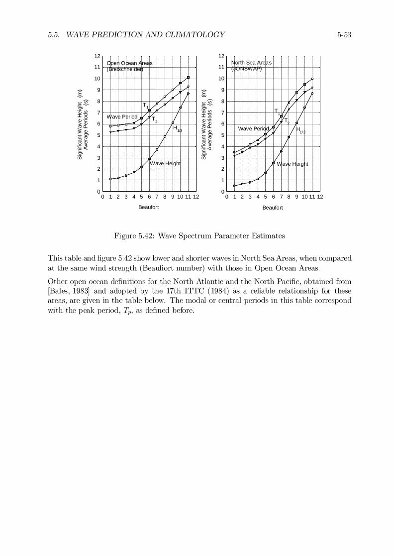
5.5. WAVE PREDICTION AND CLIMATOLOGY 5-53
0
1
2
3
4
5
6
7
8
9
10
11
12
0 1 2 3 4 5 6 7 8 9 10 11 12
H1/3
T2
T1
North Sea Areas(JONSWAP)
Wave Period
Wave Height
Beaufort
Sig
nifi
cant
Wav
e H
eigh
t (
m)
Ave
rage
Pe
riods
(s
)
0
1
2
3
4
5
6
7
8
9
10
11
12
0 1 2 3 4 5 6 7 8 9 10 11 12
H1/3
T2
T1
Open Ocean Areas(Bretschneider)
Wave Period
Wave Height
Beaufort
Sig
nific
ant W
ave
Hei
ght
(m
) A
vera
ge P
erio
ds
(s)
Figure 5.42: Wave Spectrum Parameter Estimates
This table and …gure 5.42 show lower and shorter waves in North Sea Areas, when comparedat the same wind strength (Beau…ort number) with those in Open Ocean Areas.
Other open ocean de…nitions for the North Atlantic and the North Paci…c, obtained from[Bales, 1983] and adopted by the 17th ITTC (1984) as a reliable relationship for theseareas, are given in the table below. The modal or central periods in this table correspondwith the peak period, Tp, as de…ned before.
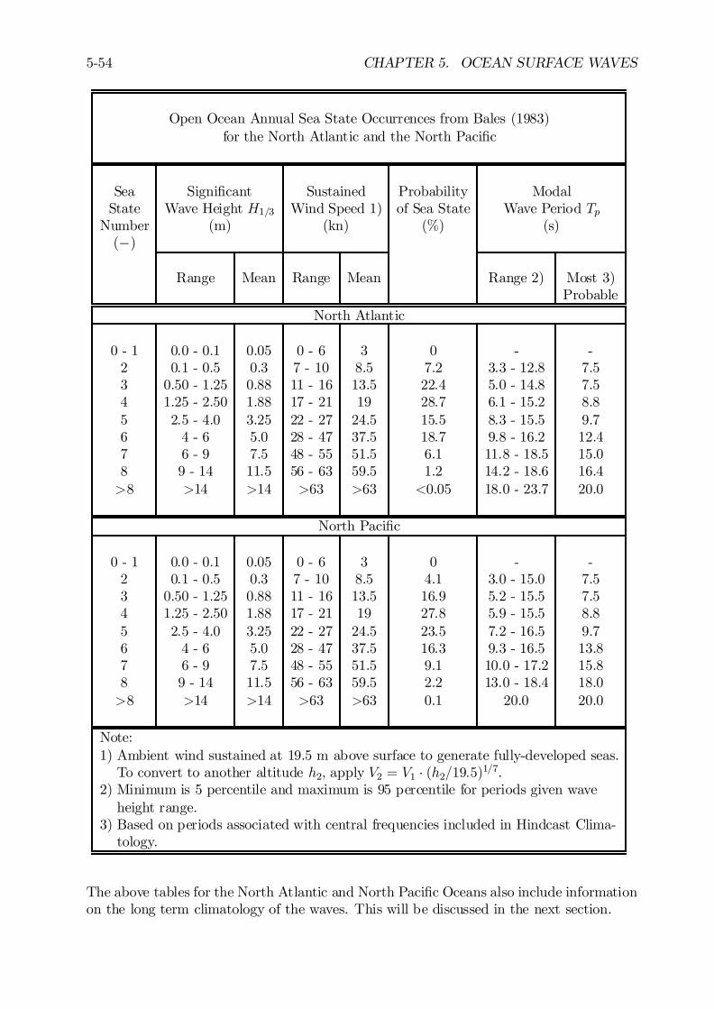
5-54 CHAPTER 5. OCEAN SURFACE WAVES
Open Ocean Annual Sea State Occurrences from Bales (1983)for the North Atlantic and the North Paci…c
Sea Signi…cant Sustained Probability ModalState Wave Height H1=3 Wind Speed 1) of Sea State Wave Period Tp
Number (m) (kn) (%) (s)(¡)
Range Mean Range Mean Range 2) Most 3)Probable
North Atlantic
0 - 1 0.0 - 0.1 0.05 0 - 6 3 0 - -2 0.1 - 0.5 0.3 7 - 10 8.5 7.2 3.3 - 12.8 7.53 0.50 - 1.25 0.88 11 - 16 13.5 22.4 5.0 - 14.8 7.54 1.25 - 2.50 1.88 17 - 21 19 28.7 6.1 - 15.2 8.85 2.5 - 4.0 3.25 22 - 27 24.5 15.5 8.3 - 15.5 9.76 4 - 6 5.0 28 - 47 37.5 18.7 9.8 - 16.2 12.47 6 - 9 7.5 48 - 55 51.5 6.1 11.8 - 18.5 15.08 9 - 14 11.5 56 - 63 59.5 1.2 14.2 - 18.6 16.4>8 >14 >14 >63 >63 <0.05 18.0 - 23.7 20.0
North Paci…c
0 - 1 0.0 - 0.1 0.05 0 - 6 3 0 - -2 0.1 - 0.5 0.3 7 - 10 8.5 4.1 3.0 - 15.0 7.53 0.50 - 1.25 0.88 11 - 16 13.5 16.9 5.2 - 15.5 7.54 1.25 - 2.50 1.88 17 - 21 19 27.8 5.9 - 15.5 8.85 2.5 - 4.0 3.25 22 - 27 24.5 23.5 7.2 - 16.5 9.76 4 - 6 5.0 28 - 47 37.5 16.3 9.3 - 16.5 13.87 6 - 9 7.5 48 - 55 51.5 9.1 10.0 - 17.2 15.88 9 - 14 11.5 56 - 63 59.5 2.2 13.0 - 18.4 18.0>8 >14 >14 >63 >63 0.1 20.0 20.0
Note:1) Ambient wind sustained at 19.5 m above surface to generate fully-developed seas.
To convert to another altitude h2, apply V2 = V1 ¢ (h2=19:5)1=7.2) Minimum is 5 percentile and maximum is 95 percentile for periods given wave
height range.3) Based on periods associated with central frequencies included in Hindcast Clima-
tology.
The above tables for the North Atlantic and North Paci…c Oceans also include informationon the long term climatology of the waves. This will be discussed in the next section.
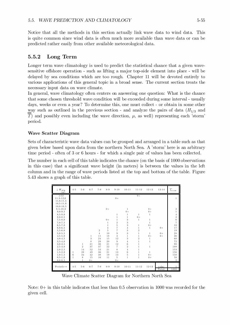
5.5. WAVE PREDICTION AND CLIMATOLOGY 5-55
Notice that all the methods in this section actually link wave data to wind data. Thisis quite common since wind data is often much more available than wave data or can bepredicted rather easily from other available meteorological data.
5.5.2 Long Term
Longer term wave climatology is used to predict the statistical chance that a given wave-sensitive o¤shore operation - such as lifting a major top-side element into place - will bedelayed by sea conditions which are too rough. Chapter 11 will be devoted entirely tovarious applications of this general topic in a broad sense. The current section treats thenecessary input data on wave climate.In general, wave climatology often centers on answering one question: What is the chancethat some chosen threshold wave condition will be exceeded during some interval - usuallydays, weeks or even a year? To determine this, one must collect - or obtain in some otherway such as outlined in the previous section - and analyze the pairs of data (H1=3 andT) and possibly even including the wave direction, ¹, as well) representing each ’storm’period.
Wave Scatter Diagram
Sets of characteristic wave data values can be grouped and arranged in a table such as thatgiven below based upon data from the northern North Sea. A ’storm’ here is an arbitrarytime period - often of 3 or 6 hours - for which a single pair of values has been collected.
The number in each cell of this table indicates the chance (on the basis of 1000 observationsin this case) that a signi…cant wave height (in meters) is between the values in the leftcolumn and in the range of wave periods listed at the top and bottom of the table. Figure5.43 shows a graph of this table.
# Hsig( m )
4 -5 5 -6 6 -7 7 -8 8 -9 9 -10 10 -11 11- 12 12 -13 13 -14P
r ow
>12 0+11 ,5- 12 ,0 0+ 111,0 -11 ,510,5 -11 ,010,0 -10 ,59 ,5 -10 ,0 0+ 1 0+ 29,0 -9 ,5 0+ 0+ 18,5 -9 ,0 1 1 1 1 48,0 -8 ,5 1 1 0+ 27,5 -8 ,0 0+ 1 3 1 1 67,0 -7 ,5 1 2 3 1 76,5 -7 ,0 1 5 3 1 0+ 106,0 -6 ,5 4 7 4 1 1 0+ 175,5 -6 ,0 2 5 7 3 2 195,0 -5 ,5 4 10 9 3 1 1 0+ 284,5 -5 ,0 1 11 18 3 1 1 0+ 0+ 364,0 -4 ,5 3 24 15 12 3 2 1 603,5 -4 ,0 8 29 20 9 4 1 1 723,0 -3 ,5 1 21 36 21 12 6 1 982,5 -3 ,0 2 37 37 22 7 2 1 1 1092,0 -2 ,5 14 52 53 21 8 4 1 1531,5 -2 ,0 1 28 49 36 21 13 6 1 1 1561,0 -1 ,5 6 34 42 38 19 13 5 1 0+ 1580,5 -1 ,0 1 8 15 16 11 5 1 1 0+ 580,0 -0 ,5 1 0+ 0+ 2
Pe riod s! 4 -5 5 -6 6 -7 7 -8 8 -9 9 -10 10 -11 11- 12 12 -13 c a lm : 1Tota l: 1000
Wave Climate Scatter Diagram for Northern North Sea
Note: 0+ in this table indicates that less than 0.5 observation in 1000 was recorded for thegiven cell.
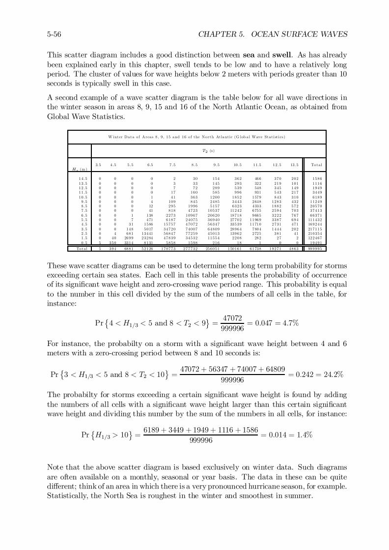
5-56 CHAPTER 5. OCEAN SURFACE WAVES
This scatter diagram includes a good distinction between sea and swell. As has alreadybeen explained early in this chapter, swell tends to be low and to have a relatively longperiod. The cluster of values for wave heights below 2 meters with periods greater than 10seconds is typically swell in this case.
A second example of a wave scatter diagram is the table below for all wave directions inthe winter season in areas 8, 9, 15 and 16 of the North Atlantic Ocean, as obtained fromGlobal Wave Statistics.
W inter Data o f Areas 8 , 9 , 15 and 16 o f the North Atlant ic (G lob a l Wave Stat ist ics)
T2 (s)
3.5 4 .5 5 .5 6 .5 7 .5 8 .5 9 .5 10 .5 11 .5 12 .5 13 .5 Tota lHs (m )
14 .5 0 0 0 0 2 30 154 362 466 370 202 158613 .5 0 0 0 0 3 33 145 293 322 219 101 111612 .5 0 0 0 0 7 72 289 539 548 345 149 194911 .5 0 0 0 0 17 160 585 996 931 543 217 344910 .5 0 0 0 1 41 363 1200 1852 1579 843 310 61899 .5 0 0 0 4 109 845 2485 3443 2648 1283 432 112498 .5 0 0 0 12 295 1996 5157 6323 4333 1882 572 205707 .5 0 0 0 41 818 4723 10537 11242 6755 2594 703 374136 .5 0 0 1 138 2273 10967 20620 18718 9665 3222 767 663715 .5 0 0 7 471 6187 24075 36940 27702 11969 3387 694 1114324 .5 0 0 31 1586 15757 47072 56347 33539 11710 2731 471 1692443 .5 0 0 148 5017 34720 74007 64809 28964 7804 1444 202 2171152 .5 0 4 681 13441 56847 77259 45013 13962 2725 381 41 2103541 .5 0 40 2699 23284 47839 34532 11554 2208 282 27 2 1224670 .5 5 350 3314 8131 5858 1598 216 18 1 0 0 19491
Tota l 5 394 6881 52126 170773 277732 256051 150161 61738 19271 4863 999995
These wave scatter diagrams can be used to determine the long term probability for stormsexceeding certain sea states. Each cell in this table presents the probability of occurrenceof its signi…cant wave height and zero-crossing wave period range. This probability is equalto the number in this cell divided by the sum of the numbers of all cells in the table, forinstance:
Pr©4 < H1=3 < 5 and 8 < T2 < 9
ª=47072
999996= 0:047 = 4:7%
For instance, the probabilty on a storm with a signi…cant wave height between 4 and 6meters with a zero-crossing period between 8 and 10 seconds is:
Pr©3 < H1=3 < 5 and 8 < T2 < 10
ª=47072 + 56347 + 74007 + 64809
999996= 0:242 = 24:2%
The probabilty for storms exceeding a certain signi…cant wave height is found by addingthe numbers of all cells with a signi…cant wave height larger than this certain signi…cantwave height and dividing this number by the sum of the numbers in all cells, for instance:
Pr©H1=3 > 10
ª=6189 + 3449 + 1949 + 1116 + 1586
999996= 0:014 = 1:4%
Note that the above scatter diagram is based exclusively on winter data. Such diagramsare often available on a monthly, seasonal or year basis. The data in these can be quitedi¤erent; think of an area in which there is a very pronounced hurricane season, for example.Statistically, the North Sea is roughest in the winter and smoothest in summer.

5.5. WAVE PREDICTION AND CLIMATOLOGY 5-57
5.5.3 Statistics
Just as with waves in an individual storm, one often wants to estimate the storm intensity(wave characteristics in this case) that one should associate with some chosen and verylow chance of exceedance. To do this one will usually have to extrapolate the wave datacollected as in the scatter diagrams above. Two statistical distribution can be used to dothis; they are described individually here.
Semi-Logarithmic Distribution
It has been found empirically that storm data - such as that presented in the wave scatterdiagram for the North Sea, above, behave quite nicely if the wave height is plotted versusthe logarithm of the chance of exceedance. The processing of the data in that scatterdiagram is very analogous to that for waves in a single storm given much earlier in thischapter.The plot resulting from the North Sea is given in …gure 5.43. The graph is pretty mucha straight line for lower probabilities, that would be needed to predict extreme events bylinear extrapolation. Obviously this segment of the graph can be extrapolated to whateverlower probability one wishes to choose. This can be done using the formula:
log f(P (H )g = 1aH
in which a is related to the slope of the curve; see …gure 5.43.
Figure 5.43: Logarthmic Distribution of Data from Northern North Sea
Weibull Distribution
A generalization of the exponential distribution given above - the Weibull distribution - isoften used, too. In equation form:
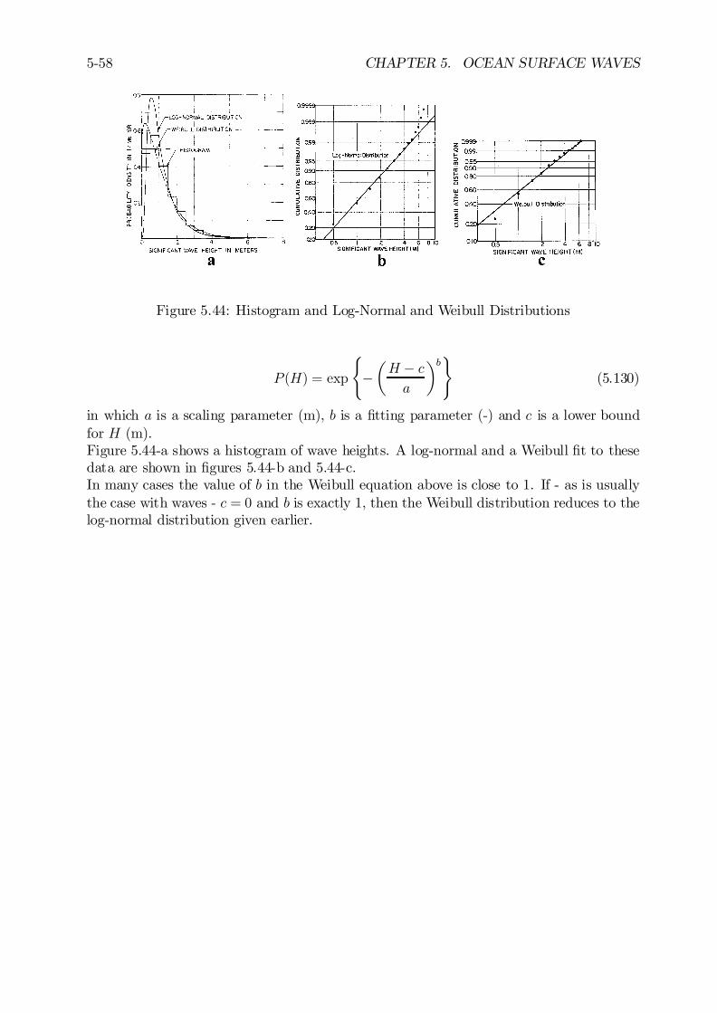
5-58 CHAPTER 5. OCEAN SURFACE WAVES
Figure 5.44: Histogram and Log-Normal and Weibull Distributions
P (H) = exp
(¡
µH ¡ ca
¶b)(5.130)
in which a is a scaling parameter (m), b is a …tting parameter (-) and c is a lower boundfor H (m).Figure 5.44-a shows a histogram of wave heights. A log-normal and a Weibull …t to thesedata are shown in …gures 5.44-b and 5.44-c.In many cases the value of b in the Weibull equation above is close to 1. If - as is usuallythe case with waves - c = 0 and b is exactly 1, then the Weibull distribution reduces to thelog-normal distribution given earlier.
Chapter 6
RIGID BODY DYNAMICS
6.1 Introduction
The dynamics of rigid bodies and ‡uid motions are governed by the combined actions ofdi¤erent external forces and moments as well as by the inertia of the bodies themselves. In‡uid dynamics these forces and moments can no longer be considered as acting at a singlepoint or at discrete points of the system. Instead, they must be regarded as distributedin a relatively smooth or a continuous manner throughout the mass of the ‡uid particles.The force and moment distributions and the kinematic description of the ‡uid motions arein fact continuous, assuming that the collection of discrete ‡uid molecules can be analyzedas a continuum.Typically, one can anticipate force mechanisms associated with the ‡uid inertia, its weight,viscous stresses and secondary e¤ects such as surface tension. In general three principalforce mechanisms (inertia, gravity and viscous) exist, which can be of comparable impor-tance. With very few exceptions, it is not possible to analyze such complicated situationsexactly - either theoretically or experimentally. It is often impossible to include all forcemechanisms simultaneously in a (mathematical) model. They can be treated in pairs ashas been done when de…ning dimensionless numbers - see chapter 4 and appendix B. Inorder to determine which pair of forces dominate, it is useful …rst to estimate the ordersof magnitude of the inertia, the gravity and the viscous forces and moments, separately.Depending on the problem, viscous e¤ects can often be ignored; this simpli…es the problemconsiderably.This chapter discusses the hydromechanics of a simple rigid body; mainly the attentionfocuses on the motions of a simple ‡oating vertical cylinder. The purpose of this chap-ter is to present much of the theory of ship motions while avoiding many of the purelyhydrodynamic complications; these are left for later chapters.
6.2 Ship De…nitions
When on board a ship looking toward the bow (front end) one is looking forward. Thestern is aft at the other end of the ship. As one looks forward, the starboard side isone’s right and the port side is to one’s left.
0J.M.J. Journée and W.W. Massie, ”OFFSHORE HYDROMECHANICS”, First Edition, January 2001,Delft University of Technology. For updates see web site: http://www.shipmotions.nl.
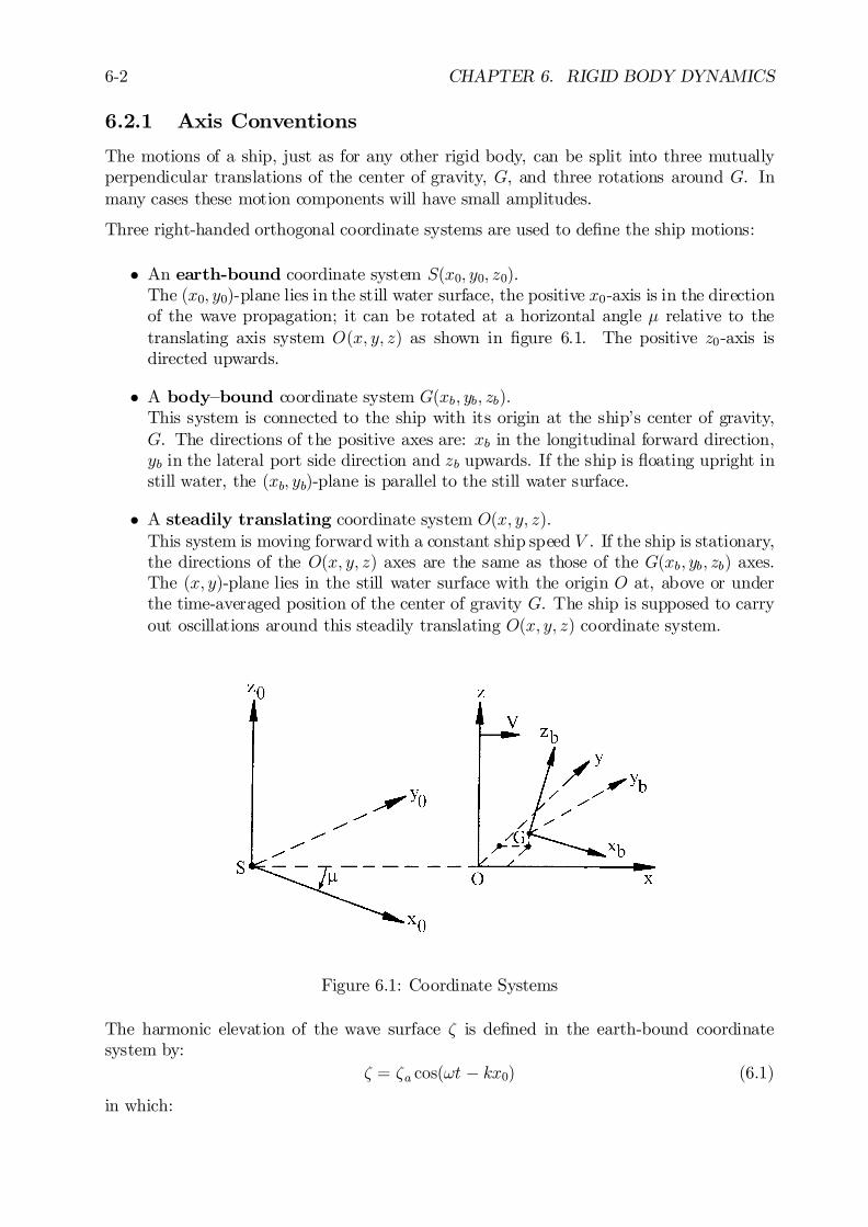
6-2 CHAPTER 6. RIGID BODY DYNAMICS
6.2.1 Axis Conventions
The motions of a ship, just as for any other rigid body, can be split into three mutuallyperpendicular translations of the center of gravity, G, and three rotations around G. Inmany cases these motion components will have small amplitudes.
Three right-handed orthogonal coordinate systems are used to de…ne the ship motions:
² An earth-bound coordinate system S(x0; y0; z0).The (x0; y0)-plane lies in the still water surface, the positive x0-axis is in the directionof the wave propagation; it can be rotated at a horizontal angle ¹ relative to thetranslating axis system O(x; y; z) as shown in …gure 6.1. The positive z0-axis isdirected upwards.
² A body–bound coordinate system G(xb; yb; zb).This system is connected to the ship with its origin at the ship’s center of gravity,G. The directions of the positive axes are: xb in the longitudinal forward direction,yb in the lateral port side direction and zb upwards. If the ship is ‡oating upright instill water, the (xb; yb)-plane is parallel to the still water surface.
² A steadily translating coordinate system O(x; y; z).This system is moving forward with a constant ship speed V . If the ship is stationary,the directions of the O(x; y; z) axes are the same as those of the G(xb; yb; zb) axes.The (x; y)-plane lies in the still water surface with the origin O at, above or underthe time-averaged position of the center of gravity G. The ship is supposed to carryout oscillations around this steadily translating O(x; y; z) coordinate system.
Figure 6.1: Coordinate Systems
The harmonic elevation of the wave surface ³ is de…ned in the earth-bound coordinatesystem by:
³ = ³a cos(!t ¡ kx0) (6.1)
in which:
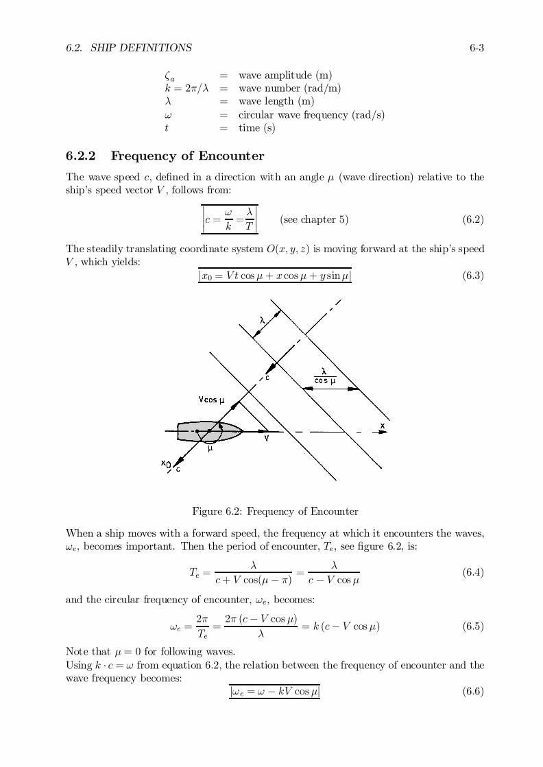
6.2. SHIP DEFINITIONS 6-3
³a = wave amplitude (m)k = 2¼=¸ = wave number (rad/m)¸ = wave length (m)! = circular wave frequency (rad/s)t = time (s)
6.2.2 Frequency of Encounter
The wave speed c, de…ned in a direction with an angle ¹ (wave direction) relative to theship’s speed vector V , follows from:
¯¯c = !
k=¸
T
¯¯ (see chapter 5) (6.2)
The steadily translating coordinate system O(x; y; z) is moving forward at the ship’s speedV , which yields:
jx0 = V t cos¹+ x cos¹+ y sin¹j (6.3)
Figure 6.2: Frequency of Encounter
When a ship moves with a forward speed, the frequency at which it encounters the waves,!e, becomes important. Then the period of encounter, Te, see …gure 6.2, is:
Te =¸
c+ V cos(¹¡ ¼) =¸
c ¡ V cos¹ (6.4)
and the circular frequency of encounter, !e, becomes:
!e =2¼
Te=2¼ (c¡ V cos¹)
¸= k (c¡ V cos¹) (6.5)
Note that ¹= 0 for following waves.Using k ¢ c = ! from equation 6.2, the relation between the frequency of encounter and thewave frequency becomes:
j!e = ! ¡ kV cos¹j (6.6)
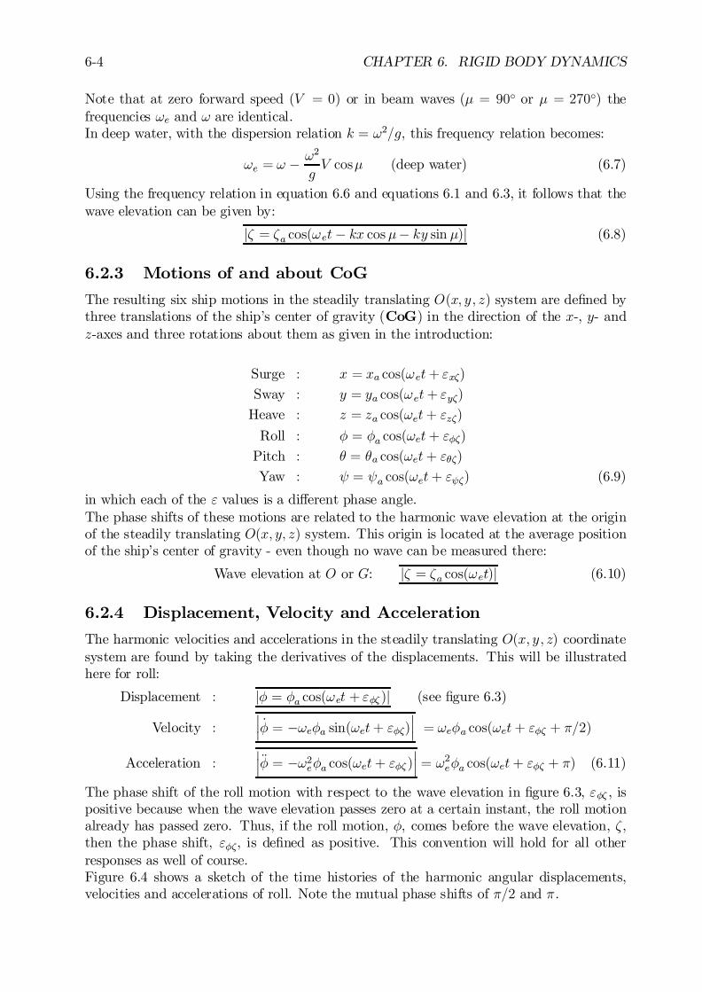
6-4 CHAPTER 6. RIGID BODY DYNAMICS
Note that at zero forward speed (V = 0) or in beam waves (¹ = 90± or ¹ = 270±) thefrequencies !e and ! are identical.In deep water, with the dispersion relation k = !2=g, this frequency relation becomes:
!e = ! ¡ !2
gV cos¹ (deep water) (6.7)
Using the frequency relation in equation 6.6 and equations 6.1 and 6.3, it follows that thewave elevation can be given by:
j³ = ³a cos(!et¡ kx cos¹¡ ky sin ¹)j (6.8)
6.2.3 Motions of and about CoG
The resulting six ship motions in the steadily translating O(x; y; z) system are de…ned bythree translations of the ship’s center of gravity (CoG) in the direction of the x-, y- andz-axes and three rotations about them as given in the introduction:
Surge : x = xa cos(!et+ "x³)
Sway : y = ya cos(!et+ "y³)
Heave : z = za cos(!et+ "z³)
Roll : Á = Áa cos(!et+ "Á³)
Pitch : µ = µa cos(!et+ "µ³)
Yaw : à = Ãa cos(!et+ "ó) (6.9)
in which each of the " values is a di¤erent phase angle.The phase shifts of these motions are related to the harmonic wave elevation at the originof the steadily translating O(x; y; z) system. This origin is located at the average positionof the ship’s center of gravity - even though no wave can be measured there:
Wave elevation at O or G: j³ = ³a cos(!et)j (6.10)
6.2.4 Displacement, Velocity and Acceleration
The harmonic velocities and accelerations in the steadily translating O(x; y; z) coordinatesystem are found by taking the derivatives of the displacements. This will be illustratedhere for roll:
Displacement : jÁ = Áa cos(!et + "Á³ )j (see …gure 6.3)
Velocity :¯¯ _Á = ¡!eÁa sin(!et+ "Á³)
¯¯ = !eÁa cos(!et+ "Á³ + ¼=2)
Acceleration :¯¯ÄÁ = ¡!2eÁa cos(!et+ "Á³ )
¯¯ = !2eÁa cos(!et+ "Á³ + ¼) (6.11)
The phase shift of the roll motion with respect to the wave elevation in …gure 6.3, "Á³ , ispositive because when the wave elevation passes zero at a certain instant, the roll motionalready has passed zero. Thus, if the roll motion, Á, comes before the wave elevation, ³,then the phase shift, "Á³, is de…ned as positive. This convention will hold for all otherresponses as well of course.Figure 6.4 shows a sketch of the time histories of the harmonic angular displacements,velocities and accelerations of roll. Note the mutual phase shifts of ¼=2 and ¼.
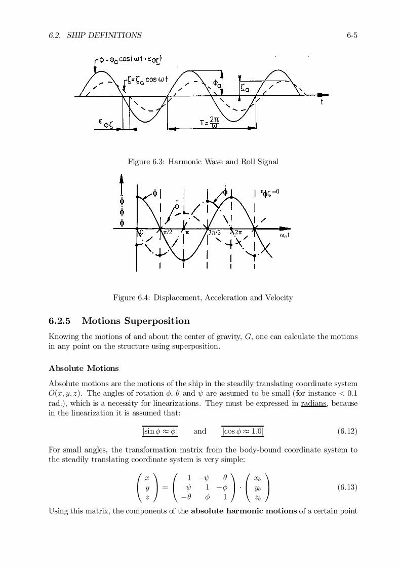
6.2. SHIP DEFINITIONS 6-5
Figure 6.3: Harmonic Wave and Roll Signal
Figure 6.4: Displacement, Acceleration and Velocity
6.2.5 Motions Superposition
Knowing the motions of and about the center of gravity, G, one can calculate the motionsin any point on the structure using superposition.
Absolute Motions
Absolute motions are the motions of the ship in the steadily translating coordinate systemO(x; y; z). The angles of rotation Á, µ and à are assumed to be small (for instance < 0.1rad.), which is a necessity for linearizations. They must be expressed in radians, becausein the linearization it is assumed that:
jsinÁ t Áj and jcos Á t 1:0j (6.12)
For small angles, the transformation matrix from the body-bound coordinate system tothe steadily translating coordinate system is very simple:
0@xyz
1A =
0@
1 ¡Ã µÃ 1 ¡Á
¡µ Á 1
1A ¢
0@xbybzb
1A (6.13)
Using this matrix, the components of the absolute harmonic motions of a certain point
6-6 CHAPTER 6. RIGID BODY DYNAMICS
P (xb; yb; zb) on the structure are given by:
jxP = x¡ ybà + zbµjjyP = y + xbà ¡ zbÁjjzP = z ¡ xbµ + ybÁ j (6.14)
in which x, y, z, Á, µ and à are the motions of and about the center of gravity, G, of thestructure.As can be seen in equation 6.14, the vertical motion, zP , in a point P (xb; yb; zb) on the‡oating structure is made up of heave, roll and pitch contributions. When looking moredetailed to this motion, it is called here now h, for convenient writing:
h (!e; t) = z ¡xbµ + ybÁ= za cos(!et+ "z³) ¡ xbµa cos(!et+ "µ³) + ybÁa cos(!et+ "Á³ )= f+za cos "z³ ¡ xbµa cos "µ³ + ybÁa cos"Á³g ¢ cos(!et)
¡f+za sin "z³ ¡ xbµa sin "µ³ + ybÁa sin "Á³g ¢ sin(!et) (6.15)
As this motion h has been obtained by a linear superposition of three harmonic motions,this (resultant) motion must be harmonic as well:
h (!e; t) = ha cos(!et+ "h³)
= fha cos "h³g ¢ cos(!et)¡ fha sin "h³g ¢ sin(!et) (6.16)
in which ha is the motion amplitude and "h³ is the phase lag of the motion with respect tothe wave elevation at G.By equating the terms with cos(!et) in equations 6.15 and 6.16 (!et = 0, so the sin(!et)-terms are zero) one …nds the in-phase term ha cos "h³; equating the terms with sin(!et) inequations 6.15 and 6.16 (!et = ¼=2, so the cos(!et)-terms are zero) provides the out-of-phase term ha sin "h³ of the vertical displacement in P :
ha cos "h³ = +za cos "z³ ¡ xbµa cos "µ³ + ybÁa cos "Á³ha sin "h³ = +za sin "z³ ¡ xbµa sin "µ³ + ybÁa sin "Á³ (6.17)
Since the right hand sides of equations 6.17 are known, the amplitude ha and phase shift"h³ become:
¯¯ha =
q(ha sin "h³)
2 + (ha cos "h³ )2
¯¯
¯¯"h³ = arctan
½ha sin "h³ha cos "h³
¾with: 0 · "h³ · 2¼
¯¯ (6.18)
The phase angle "h³ has to be determined in the correct quadrant between 0 and 2¼. Thisdepends on the signs of both the numerator and the denominator in the expression forthe arctangent. If the phase shift "h³ has been determined between ¡¼=2 and +¼=2 andha cos "h³ is negative, then ¼ should be added or subtracted from this "h³ to obtain thecorrect phase shift.
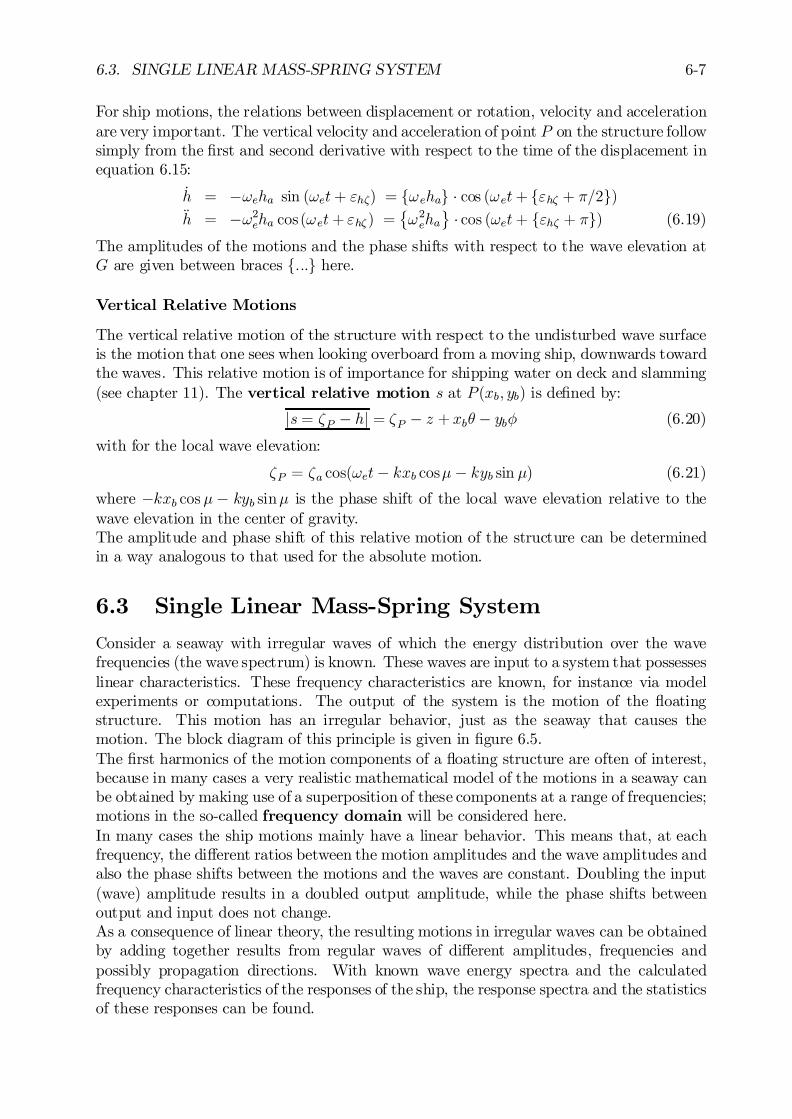
6.3. SINGLE LINEAR MASS-SPRING SYSTEM 6-7
For ship motions, the relations between displacement or rotation, velocity and accelerationare very important. The vertical velocity and acceleration of point P on the structure followsimply from the …rst and second derivative with respect to the time of the displacement inequation 6.15:
_h = ¡!eha sin (!et+ "h³) = f!ehag ¢ cos (!et+ f"h³ + ¼=2g)Äh = ¡!2eha cos(!et+ "h³ ) =
©!2eha
ª¢ cos (!et+ f"h³ + ¼g) (6.19)
The amplitudes of the motions and the phase shifts with respect to the wave elevation atG are given between braces f:::g here.
Vertical Relative Motions
The vertical relative motion of the structure with respect to the undisturbed wave surfaceis the motion that one sees when looking overboard from a moving ship, downwards towardthe waves. This relative motion is of importance for shipping water on deck and slamming(see chapter 11). The vertical relative motion s at P (xb; yb) is de…ned by:
js= ³P ¡ hj = ³P ¡ z + xbµ¡ ybÁ (6.20)
with for the local wave elevation:
³P = ³a cos(!et¡ kxb cos¹¡ kyb sin ¹) (6.21)
where ¡kxb cos¹¡ kyb sin¹ is the phase shift of the local wave elevation relative to thewave elevation in the center of gravity.The amplitude and phase shift of this relative motion of the structure can be determinedin a way analogous to that used for the absolute motion.
6.3 Single Linear Mass-Spring System
Consider a seaway with irregular waves of which the energy distribution over the wavefrequencies (the wave spectrum) is known. These waves are input to a system that possesseslinear characteristics. These frequency characteristics are known, for instance via modelexperiments or computations. The output of the system is the motion of the ‡oatingstructure. This motion has an irregular behavior, just as the seaway that causes themotion. The block diagram of this principle is given in …gure 6.5.The …rst harmonics of the motion components of a ‡oating structure are often of interest,because in many cases a very realistic mathematical model of the motions in a seaway canbe obtained by making use of a superposition of these components at a range of frequencies;motions in the so-called frequency domain will be considered here.In many cases the ship motions mainly have a linear behavior. This means that, at eachfrequency, the di¤erent ratios between the motion amplitudes and the wave amplitudes andalso the phase shifts between the motions and the waves are constant. Doubling the input(wave) amplitude results in a doubled output amplitude, while the phase shifts betweenoutput and input does not change.As a consequence of linear theory, the resulting motions in irregular waves can be obtainedby adding together results from regular waves of di¤erent amplitudes, frequencies andpossibly propagation directions. With known wave energy spectra and the calculatedfrequency characteristics of the responses of the ship, the response spectra and the statisticsof these responses can be found.
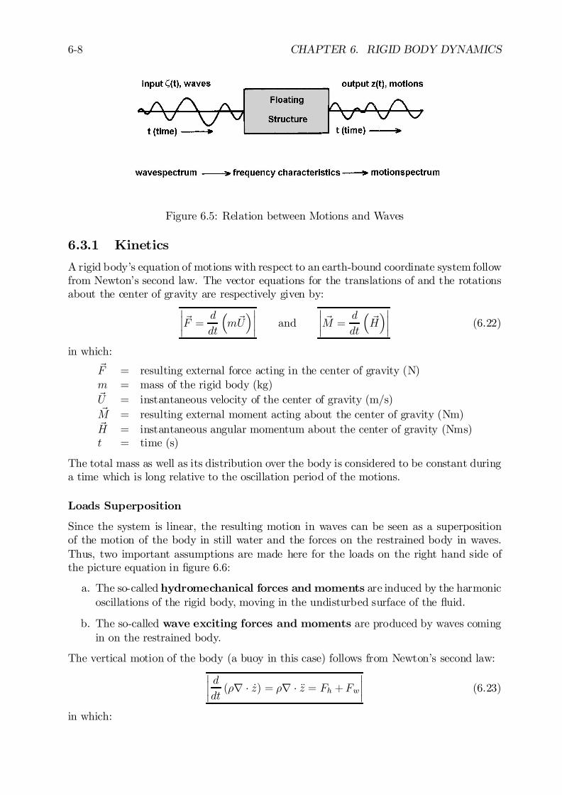
6-8 CHAPTER 6. RIGID BODY DYNAMICS
Figure 6.5: Relation between Motions and Waves
6.3.1 Kinetics
A rigid body’s equation of motions with respect to an earth-bound coordinate system followfrom Newton’s second law. The vector equations for the translations of and the rotationsabout the center of gravity are respectively given by:
¯¯~F = d
dt
³m~U
´¯¯ and
¯¯ ~M =
d
dt
³~H
´¯¯ (6.22)
in which:
~F = resulting external force acting in the center of gravity (N)m = mass of the rigid body (kg)~U = instantaneous velocity of the center of gravity (m/s)~M = resulting external moment acting about the center of gravity (Nm)~H = instantaneous angular momentum about the center of gravity (Nms)t = time (s)
The total mass as well as its distribution over the body is considered to be constant duringa time which is long relative to the oscillation period of the motions.
Loads Superposition
Since the system is linear, the resulting motion in waves can be seen as a superpositionof the motion of the body in still water and the forces on the restrained body in waves.Thus, two important assumptions are made here for the loads on the right hand side ofthe picture equation in …gure 6.6:
a. The so-called hydromechanical forces and moments are induced by the harmonicoscillations of the rigid body, moving in the undisturbed surface of the ‡uid.
b. The so-called wave exciting forces and moments are produced by waves comingin on the restrained body.
The vertical motion of the body (a buoy in this case) follows from Newton’s second law:¯¯ ddt(½r ¢ _z) = ½r ¢ Äz = Fh +Fw
¯¯ (6.23)
in which:
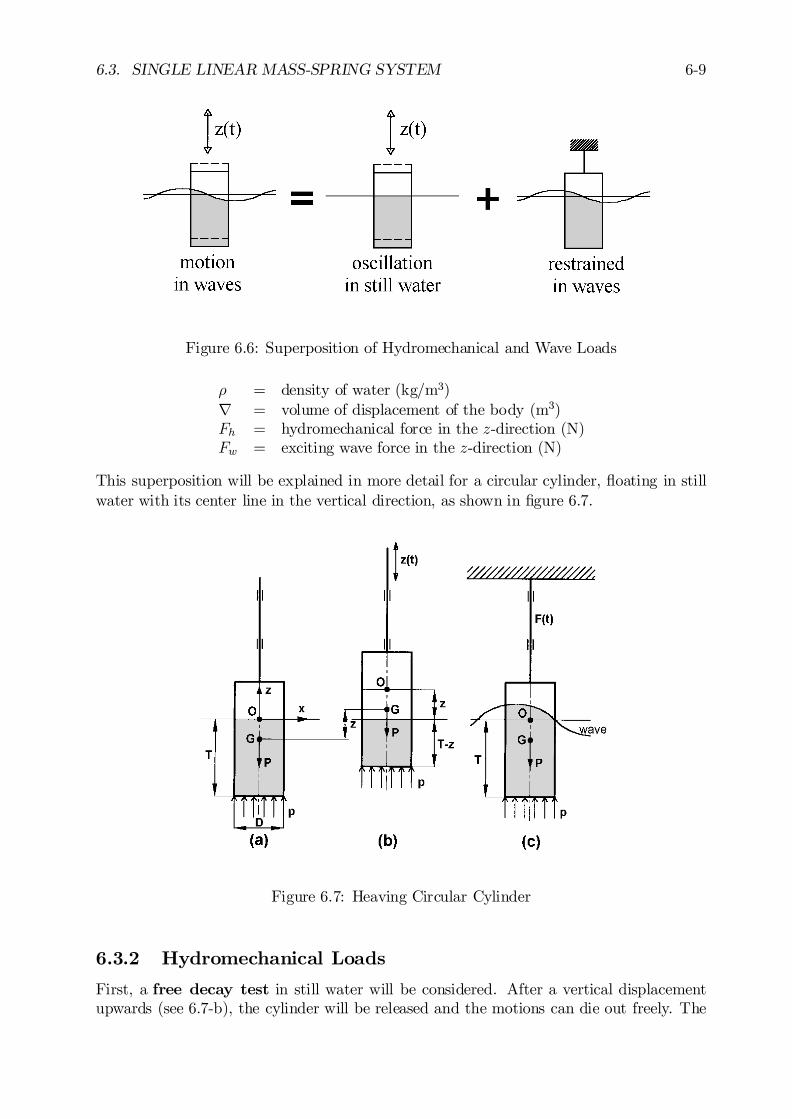
6.3. SINGLE LINEAR MASS-SPRING SYSTEM 6-9
Figure 6.6: Superposition of Hydromechanical and Wave Loads
½ = density of water (kg/m3)r = volume of displacement of the body (m3)Fh = hydromechanical force in the z-direction (N)Fw = exciting wave force in the z-direction (N)
This superposition will be explained in more detail for a circular cylinder, ‡oating in stillwater with its center line in the vertical direction, as shown in …gure 6.7.
Figure 6.7: Heaving Circular Cylinder
6.3.2 Hydromechanical Loads
First, a free decay test in still water will be considered. After a vertical displacementupwards (see 6.7-b), the cylinder will be released and the motions can die out freely. The
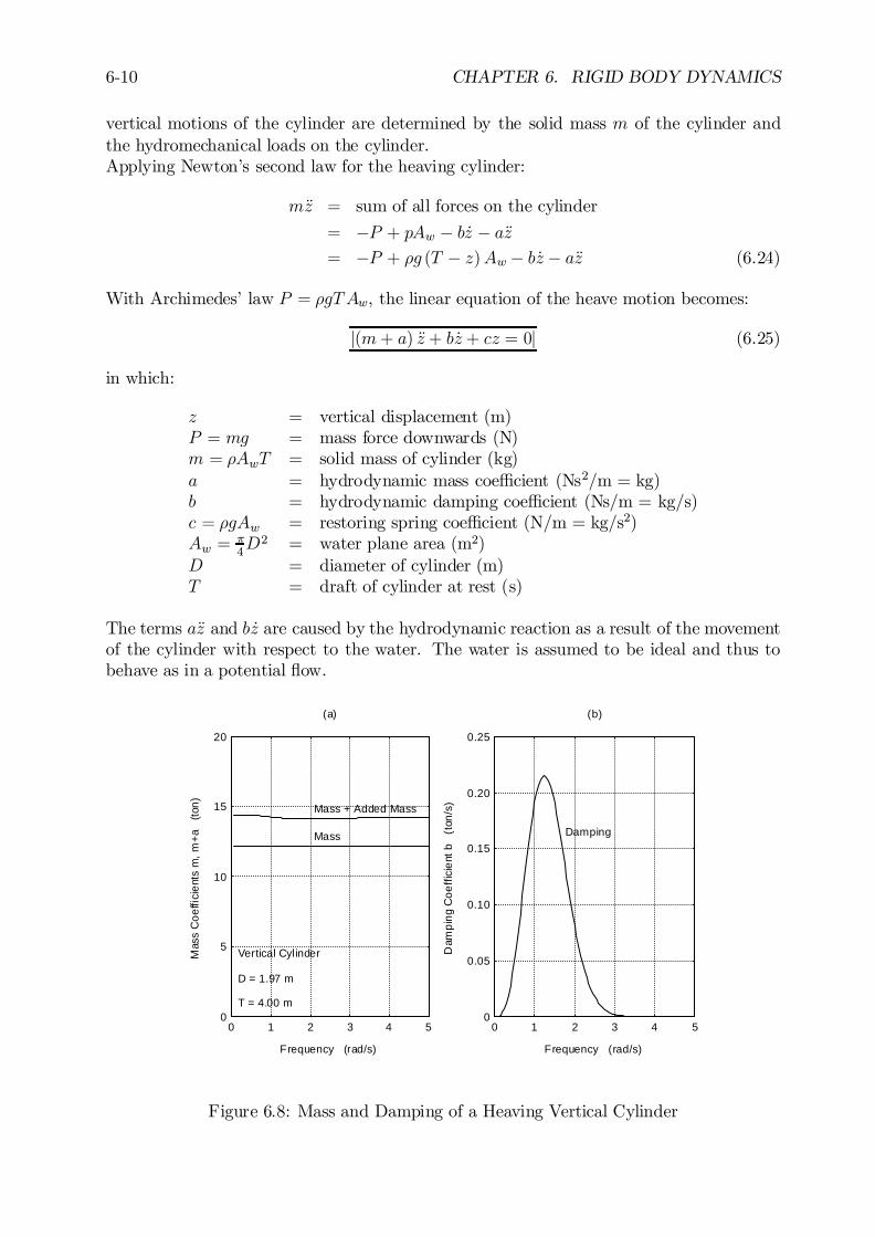
6-10 CHAPTER 6. RIGID BODY DYNAMICS
vertical motions of the cylinder are determined by the solid mass m of the cylinder andthe hydromechanical loads on the cylinder.Applying Newton’s second law for the heaving cylinder:
mÄz = sum of all forces on the cylinder
= ¡P + pAw ¡ b _z ¡ aÄz= ¡P + ½g (T ¡ z)Aw ¡ b _z ¡ aÄz (6.24)
With Archimedes’ law P = ½gTAw, the linear equation of the heave motion becomes:
j(m+ a) Äz + b _z + cz = 0j (6.25)
in which:
z = vertical displacement (m)P = mg = mass force downwards (N)m = ½AwT = solid mass of cylinder (kg)a = hydrodynamic mass coe¢cient (Ns2/m = kg)b = hydrodynamic damping coe¢cient (Ns/m = kg/s)c = ½gAw = restoring spring coe¢cient (N/m = kg/s2)Aw =
¼4D2 = water plane area (m2)
D = diameter of cylinder (m)T = draft of cylinder at rest (s)
The terms aÄz and b _z are caused by the hydrodynamic reaction as a result of the movementof the cylinder with respect to the water. The water is assumed to be ideal and thus tobehave as in a potential ‡ow.
0
5
10
15
20
0 1 2 3 4 5
Vertical Cylinder D = 1.97 m T = 4.00 m
Mass + Added Mass
Mass
Frequency (rad/s)
Mas
s C
oeffi
cien
ts m
, m+a
(to
n)
(a)
0
0.05
0.10
0.15
0.20
0.25
0 1 2 3 4 5
Damping
Frequency (rad/s)
Dam
ping
Coe
ffici
ent b
(t
on/s
)
(b)
Figure 6.8: Mass and Damping of a Heaving Vertical Cylinder
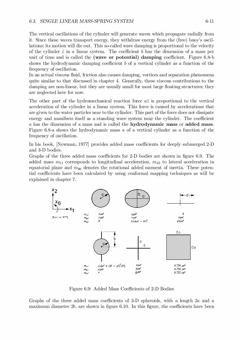
6.3. SINGLE LINEAR MASS-SPRING SYSTEM 6-11
The vertical oscillations of the cylinder will generate waves which propagate radially fromit. Since these waves transport energy, they withdraw energy from the (free) buoy’s oscil-lations; its motion will die out. This so-called wave damping is proportional to the velocityof the cylinder _z in a linear system. The coe¢cient b has the dimension of a mass perunit of time and is called the (wave or potential) damping coe¢cient. Figure 6.8-bshows the hydrodynamic damping coe¢cient b of a vertical cylinder as a function of thefrequency of oscillation.In an actual viscous ‡uid, friction also causes damping, vortices and separation phenomenaquite similar to that discussed in chapter 4. Generally, these viscous contributions to thedamping are non-linear, but they are usually small for most large ‡oating structures; theyare neglected here for now.
The other part of the hydromechanical reaction force aÄz is proportional to the verticalacceleration of the cylinder in a linear system. This force is caused by accelerations thatare given to the water particles near to the cylinder. This part of the force does not dissipateenergy and manifests itself as a standing wave system near the cylinder. The coe¢cienta has the dimension of a mass and is called the hydrodynamic mass or added mass.Figure 6.8-a shows the hydrodynamic mass a of a vertical cylinder as a function of thefrequency of oscillation.
In his book, [Newman, 1977] provides added mass coe¢cients for deeply submerged 2-Dand 3-D bodies.Graphs of the three added mass coe¢cients for 2-D bodies are shown in …gure 6.9. Theadded mass m11 corresponds to longitudinal acceleration, m22 to lateral acceleration inequatorial plane and m66 denotes the rotational added moment of inertia. These poten-tial coe¢cients have been calculated by using conformal mapping techniques as will beexplained in chapter 7.
Figure 6.9: Added Mass Coe¢cients of 2-D Bodies
Graphs of the three added mass coe¢cients of 3-D spheroids, with a length 2a and amaximum diameter 2b, are shown in …gure 6.10. In this …gure, the coe¢cients have been
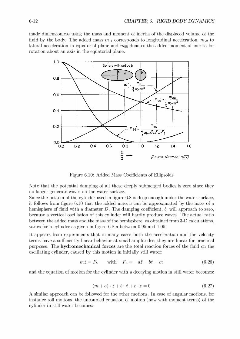
6-12 CHAPTER 6. RIGID BODY DYNAMICS
made dimensionless using the mass and moment of inertia of the displaced volume of the‡uid by the body. The added mass m11 corresponds to longitudinal acceleration, m22 tolateral acceleration in equatorial plane and m55 denotes the added moment of inertia forrotation about an axis in the equatorial plane.
Figure 6.10: Added Mass Coe¢cients of Ellipsoids
Note that the potential damping of all these deeply submerged bodies is zero since theyno longer generate waves on the water surface.Since the bottom of the cylinder used in …gure 6.8 is deep enough under the water surface,it follows from …gure 6.10 that the added mass a can be approximated by the mass of ahemisphere of ‡uid with a diameter D. The damping coe¢cient, b, will approach to zero,because a vertical oscillation of this cylinder will hardly produce waves. The actual ratiobetween the added mass and the mass of the hemisphere, as obtained from 3-D calculations,varies for a cylinder as given in …gure 6.8-a between 0.95 and 1.05.
It appears from experiments that in many cases both the acceleration and the velocityterms have a su¢ciently linear behavior at small amplitudes; they are linear for practicalpurposes. The hydromechanical forces are the total reaction forces of the ‡uid on theoscillating cylinder, caused by this motion in initially still water:
mÄz = Fh with: Fh = ¡aÄz ¡ b _z ¡ cz (6.26)
and the equation of motion for the cylinder with a decaying motion in still water becomes:
(m+ a) ¢ Äz + b ¢ _z + c ¢ z = 0 (6.27)
A similar approach can be followed for the other motions. In case of angular motions, forinstance roll motions, the uncoupled equation of motion (now with moment terms) of thecylinder in still water becomes:
6.3. SINGLE LINEAR MASS-SPRING SYSTEM 6-13
(m+ a) ¢ ÄÁ + b ¢ _Á + c ¢ Á = 0 (6.28)
and the coe¢cients in the acceleration term, a and m, are (added) mass moment of inertiaterms. Coupling between motions will be discussed in chapter 8.
Energy Relations
Suppose the cylinder is carrying out a vertical harmonic oscillation:
z = za sin!t
in initially still water of which the linear equation of motion is given by equation 6.27.The separate work done by the mass, damping and spring force components in this equation(force component times distance) per unit of time during one period of oscillation, T , are:
1
T
TZ
0
f(m+ a) ¢ Äzg ¢ f _z ¢ dtg =¡za2(m+ a)!3
T
TZ
0
sin!t ¢ cos!t ¢ dt = 0
1
T
TZ
0
fb ¢ _zg ¢ f _z ¢ dtg =za2b!2
T
TZ
0
cos2 !t ¢ dt = 12b !2za
2
1
T
TZ
0
fc ¢ zg ¢ f _z ¢ dtg =za2c!
T
TZ
0
sin!t ¢ cos!t ¢ dt = 0 (6.29)
with:
T = 2¼=! = oscillation period (s)_z ¢ dt = dz = distance covered in dt seconds (m)
It is obvious from these equations that only the damping force fb ¢ _zg dissipates energy;damping is the reason why the heave motion, z, dies out.Observe now a ‡oating horizontal cylinder as given in …gure 6.11, carrying out a verticalharmonic oscillation in initially still water: z = za sin!t, which causes radiated wavesde…ned by: ³ = ³a sin(!t + "). A frequency-dependent relation between the dampingcoe¢cient, b, and the amplitude ratio of radiated waves and the vertical oscillation, ³a=za,can be found; see also [Newman, 1962].The energy E (the work done per unit of time) provided by the hydrodynamic dampingforce is the over one period (T ) integrated damping force (b ¢ _z) times covered distance( _z ¢ dt) divided by the time (T):
E =1
T
TZ
0
fb ¢ _zg ¢ f _z ¢ dtg
=1
2b!2za
2 (6.30)
This energy provided by the above mentioned hydrodynamic damping force is equal to theenergy dissipated by the radiated waves. This is 2 (radiation of waves to two sides) times
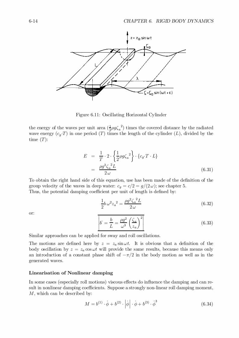
6-14 CHAPTER 6. RIGID BODY DYNAMICS
Figure 6.11: Oscillating Horizontal Cylinder
the energy of the waves per unit area ( 12½g³a
2) times the covered distance by the radiatedwave energy (cg ¢T) in one period (T) times the length of the cylinder (L), divided by thetime (T):
E =1
T¢ 2 ¢
½1
2½g³a
2
¾¢ fcg¢T ¢ Lg
=½g2³a
2L
2!(6.31)
To obtain the right hand side of this equation, use has been made of the de…nition of thegroup velocity of the waves in deep water: cg = c=2 = g=(2!); see chapter 5.Thus, the potential damping coe¢cient per unit of length is de…ned by:
1
2b !2za
2 =½g2³a
2L
2!(6.32)
or: ¯¯¯b0 =
b
L=½g2
!3
µ³aza
¶2¯¯¯ (6.33)
Similar approaches can be applied for sway and roll oscillations.
The motions are de…ned here by z = za sin!t. It is obvious that a de…nition of thebody oscillation by z = za cos!t will provide the same results, because this means onlyan introduction of a constant phase shift of ¡¼=2 in the body motion as well as in thegenerated waves.
Linearisation of Nonlinear damping
In some cases (especially roll motions) viscous e¤ects do in‡uence the damping and can re-sult in nonlinear damping coe¢cients. Suppose a strongly non-linear roll damping moment,M , which can be described by:
M = b(1) ¢ _Á + b(2) ¢¯¯ _Á
¯¯ ¢ _Á+ b(3) ¢ _Á3 (6.34)
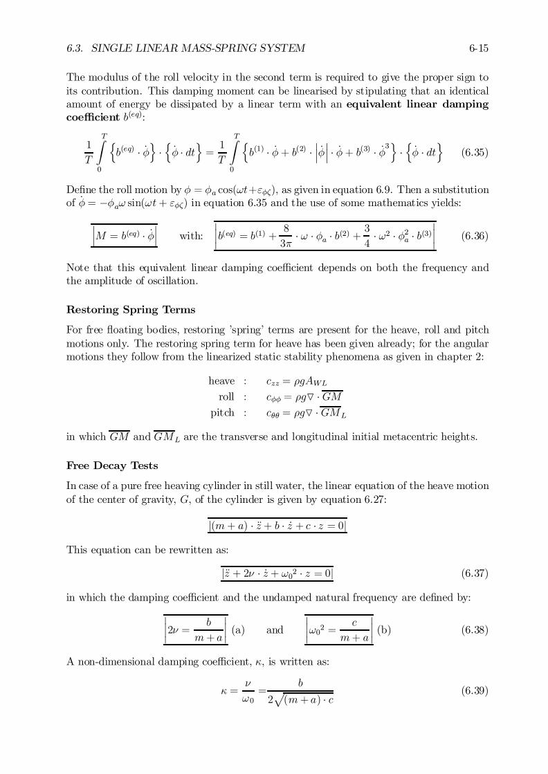
6.3. SINGLE LINEAR MASS-SPRING SYSTEM 6-15
The modulus of the roll velocity in the second term is required to give the proper sign toits contribution. This damping moment can be linearised by stipulating that an identicalamount of energy be dissipated by a linear term with an equivalent linear dampingcoe¢cient b(eq):
1
T
TZ
0
nb(eq) ¢ _Á
o¢n_Á ¢ dt
o=1
T
TZ
0
nb(1) ¢ _Á + b(2) ¢
¯¯ _Á
¯¯ ¢ _Á + b(3) ¢ _Á3
o¢n_Á ¢ dt
o(6.35)
De…ne the roll motion by Á = Áa cos(!t+"Á³), as given in equation 6.9. Then a substitutionof _Á = ¡Áa! sin(!t+ "Á³) in equation 6.35 and the use of some mathematics yields:
¯¯M = b(eq) ¢ _Á
¯¯ with:
¯¯b(eq) = b(1) + 8
3¼¢ ! ¢ Áa ¢ b(2) + 3
4¢ !2 ¢ Á2a ¢ b(3)
¯¯ (6.36)
Note that this equivalent linear damping coe¢cient depends on both the frequency andthe amplitude of oscillation.
Restoring Spring Terms
For free ‡oating bodies, restoring ’spring’ terms are present for the heave, roll and pitchmotions only. The restoring spring term for heave has been given already; for the angularmotions they follow from the linearized static stability phenomena as given in chapter 2:
heave : czz = ½gAWL
roll : cÁÁ = ½gO ¢GMpitch : cµµ = ½gO ¢GML
in which GM and GML are the transverse and longitudinal initial metacentric heights.
Free Decay Tests
In case of a pure free heaving cylinder in still water, the linear equation of the heave motionof the center of gravity, G, of the cylinder is given by equation 6.27:
j(m+ a) ¢ Äz + b ¢ _z + c ¢ z = 0j
This equation can be rewritten as:
jÄz + 2º ¢ _z + !02 ¢ z = 0j (6.37)
in which the damping coe¢cient and the undamped natural frequency are de…ned by:
¯¯2º = b
m+ a
¯¯ (a) and
¯¯!02 =
c
m+ a
¯¯ (b) (6.38)
A non-dimensional damping coe¢cient, ·, is written as:
· =º
!0=
b
2p(m+ a) ¢ c
(6.39)
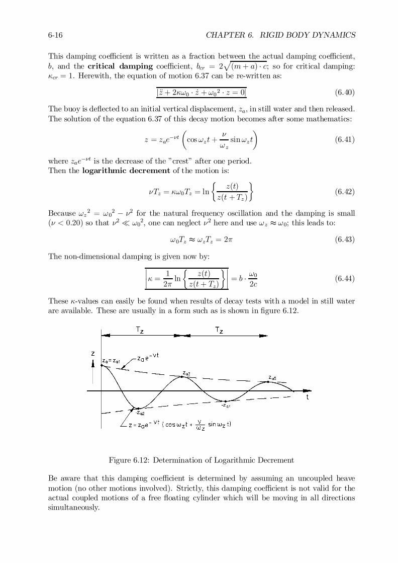
6-16 CHAPTER 6. RIGID BODY DYNAMICS
This damping coe¢cient is written as a fraction between the actual damping coe¢cient,b, and the critical damping coe¢cient, bcr = 2
p(m+ a) ¢ c; so for critical damping:
·cr = 1. Herewith, the equation of motion 6.37 can be re-written as:
jÄz + 2·!0 ¢ _z +!02 ¢ z = 0j (6.40)
The buoy is de‡ected to an initial vertical displacement, za, in still water and then released.The solution of the equation 6.37 of this decay motion becomes after some mathematics:
z = zae¡ºt
µcos!zt+
º
!zsin!zt
¶(6.41)
where zae¡ºt is the decrease of the ”crest” after one period.Then the logarithmic decrement of the motion is:
ºTz = ·!0Tz = ln
½z(t)
z(t + Tz)
¾(6.42)
Because !z2 = !02 ¡ º2 for the natural frequency oscillation and the damping is small(º < 0:20) so that º2 ¿ !02, one can neglect º2 here and use !z t !0; this leads to:
!0Tz t !zTz = 2¼ (6.43)
The non-dimensional damping is given now by:¯¯· = 1
2¼ln
½z(t)
z(t+ Tz)
¾¯¯ = b ¢ !0
2c(6.44)
These ·-values can easily be found when results of decay tests with a model in still waterare available. These are usually in a form such as is shown in …gure 6.12.
Figure 6.12: Determination of Logarithmic Decrement
Be aware that this damping coe¢cient is determined by assuming an uncoupled heavemotion (no other motions involved). Strictly, this damping coe¢cient is not valid for theactual coupled motions of a free ‡oating cylinder which will be moving in all directionssimultaneously.
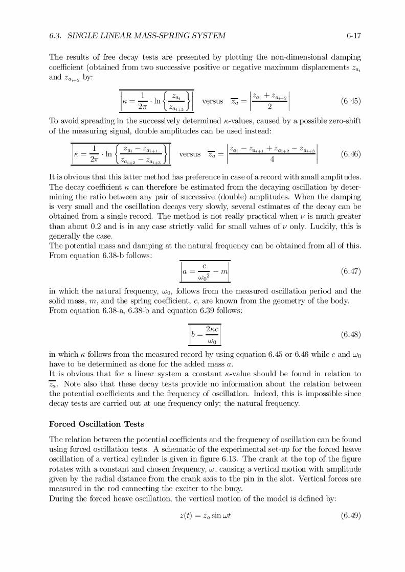
6.3. SINGLE LINEAR MASS-SPRING SYSTEM 6-17
The results of free decay tests are presented by plotting the non-dimensional dampingcoe¢cient (obtained from two successive positive or negative maximum displacements zaiand zai+2 by:
¯¯· = 1
2¼¢ ln
½zaizai+2
¾¯¯ versus za =
¯¯zai + zai+2
2
¯¯ (6.45)
To avoid spreading in the successively determined ·-values, caused by a possible zero-shiftof the measuring signal, double amplitudes can be used instead:
¯¯· = 1
2¼¢ ln
½zai ¡ zai+1zai+2 ¡ zai+3
¾¯¯ versus za =
¯¯zai ¡ zai+1 + zai+2 ¡ zai+3
4
¯¯ (6.46)
It is obvious that this latter method has preference in case of a record with small amplitudes.The decay coe¢cient · can therefore be estimated from the decaying oscillation by deter-mining the ratio between any pair of successive (double) amplitudes. When the dampingis very small and the oscillation decays very slowly, several estimates of the decay can beobtained from a single record. The method is not really practical when º is much greaterthan about 0.2 and is in any case strictly valid for small values of º only. Luckily, this isgenerally the case.The potential mass and damping at the natural frequency can be obtained from all of this.From equation 6.38-b follows: ¯
¯a = c
!02¡m
¯¯ (6.47)
in which the natural frequency, !0, follows from the measured oscillation period and thesolid mass, m, and the spring coe¢cient, c, are known from the geometry of the body.From equation 6.38-a, 6.38-b and equation 6.39 follows:
¯¯b = 2·c
!0
¯¯ (6.48)
in which · follows from the measured record by using equation 6.45 or 6.46 while c and !0have to be determined as done for the added mass a.It is obvious that for a linear system a constant ·-value should be found in relation toza. Note also that these decay tests provide no information about the relation betweenthe potential coe¢cients and the frequency of oscillation. Indeed, this is impossible sincedecay tests are carried out at one frequency only; the natural frequency.
Forced Oscillation Tests
The relation between the potential coe¢cients and the frequency of oscillation can be foundusing forced oscillation tests. A schematic of the experimental set-up for the forced heaveoscillation of a vertical cylinder is given in …gure 6.13. The crank at the top of the …gurerotates with a constant and chosen frequency, !, causing a vertical motion with amplitudegiven by the radial distance from the crank axis to the pin in the slot. Vertical forces aremeasured in the rod connecting the exciter to the buoy.During the forced heave oscillation, the vertical motion of the model is de…ned by:
z(t) = za sin !t (6.49)
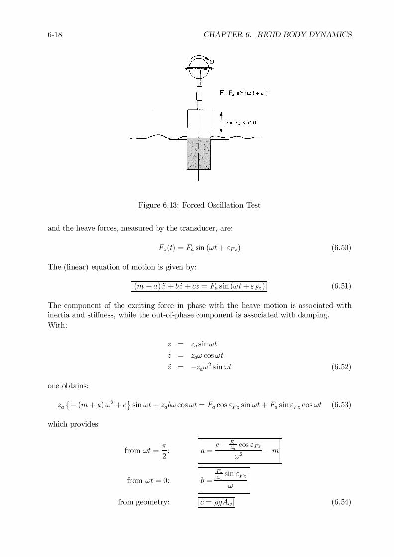
6-18 CHAPTER 6. RIGID BODY DYNAMICS
Figure 6.13: Forced Oscillation Test
and the heave forces, measured by the transducer, are:
Fz(t) = Fa sin (!t+ "Fz) (6.50)
The (linear) equation of motion is given by:
j(m + a) Äz + b _z + cz = Fa sin (!t+ "Fz)j (6.51)
The component of the exciting force in phase with the heave motion is associated withinertia and sti¤ness, while the out-of-phase component is associated with damping.With:
z = za sin!t
_z = za! cos!t
Äz = ¡za!2 sin!t (6.52)
one obtains:
za©¡ (m+ a)!2 + cª sin !t+ zab! cos!t = Fa cos "Fz sin !t+ Fa sin "Fz cos!t (6.53)
which provides:
from !t =¼
2:
¯¯¯a =
c ¡ Fazacos "Fz
!2¡m
¯¯¯
from !t = 0:
¯¯¯b =
Fazasin "Fz
!
¯¯¯
from geometry: jc = ½gAwj (6.54)
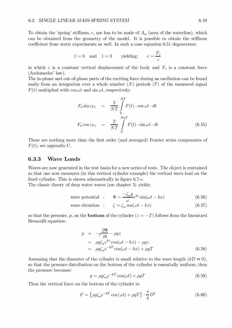
6.3. SINGLE LINEAR MASS-SPRING SYSTEM 6-19
To obtain the ’spring’ sti¤ness, c, use has to be made of Aw (area of the waterline), whichcan be obtained from the geometry of the model. It is possible to obtain the sti¤nesscoe¢cient from static experiments as well. In such a case equation 6.51 degenerates:
Äz = 0 and _z = 0 yielding: c =Fzz
in which z is a constant vertical displacement of the body and Fz is a constant force(Archimedes’ law).The in-phase and out-of-phase parts of the exciting force during an oscillation can be foundeasily from an integration over a whole number (N ) periods (T) of the measured signalF (t) multiplied with cos!t and sin !t, respectively:
Fa sin "Fz =2
NT
NTZ
0
F (t) ¢ cos!t ¢ dt
Fa cos "Fz =2
NT
NnTZ
0
F (t) ¢ sin!t ¢ dt (6.55)
These are nothing more than the …rst order (and averaged) Fourier series components ofF (t); see appendix C:
6.3.3 Wave Loads
Waves are now generated in the test basin for a new series of tests. The object is restrainedso that one now measures (in this vertical cylinder example) the vertical wave load on the…xed cylinder. This is shown schematically in …gure 6.7-c.The classic theory of deep water waves (see chapter 5) yields:
wave potential : © =¡³ag!
ekz sin(!t¡ kx) (6.56)
wave elevation : ³ = ³a cos(!t¡ kx) (6.57)
so that the pressure, p, on the bottom of the cylinder (z = ¡T) follows from the linearizedBernoulli equation:
p = ¡½@©@t
¡ ½gz= ½g³ae
kz cos(!t ¡ kx) ¡ ½gz= ½g³ae
¡kT cos(!t¡ kx) + ½gT (6.58)
Assuming that the diameter of the cylinder is small relative to the wave length (kD t 0),so that the pressure distribution on the bottom of the cylinder is essentially uniform, thenthe pressure becomes:
p = ½g³ae¡kT cos(!t) + ½gT (6.59)
Then the vertical force on the bottom of the cylinder is:
F =©½g³ae
¡kT cos(!t) + ½gTª
¢ ¼4D2 (6.60)
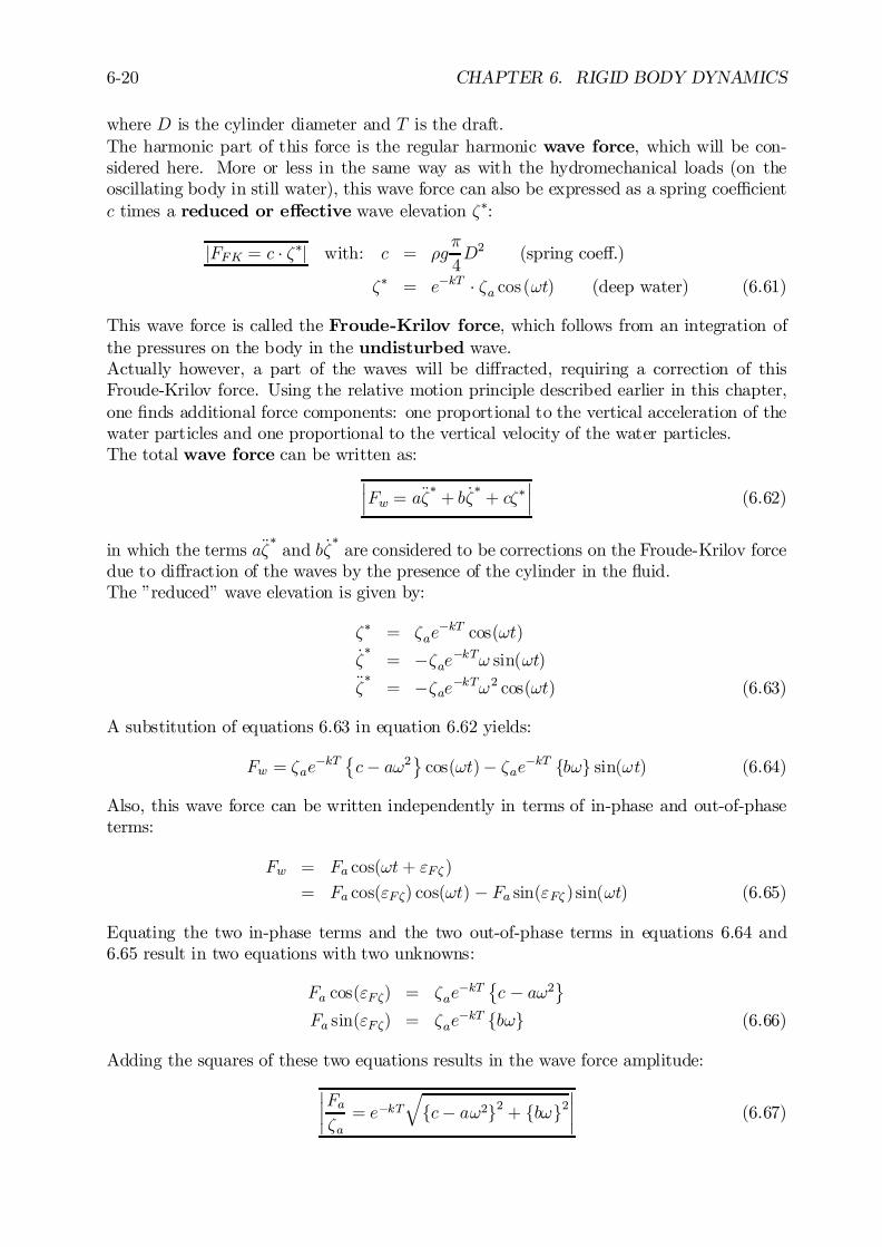
6-20 CHAPTER 6. RIGID BODY DYNAMICS
where D is the cylinder diameter and T is the draft.The harmonic part of this force is the regular harmonic wave force, which will be con-sidered here. More or less in the same way as with the hydromechanical loads (on theoscillating body in still water), this wave force can also be expressed as a spring coe¢cientc times a reduced or e¤ective wave elevation ³¤:
jFFK = c ¢ ³¤j with: c = ½g¼
4D2 (spring coe¤.)
³¤ = e¡kT ¢ ³a cos(!t) (deep water) (6.61)
This wave force is called the Froude-Krilov force, which follows from an integration ofthe pressures on the body in the undisturbed wave.Actually however, a part of the waves will be di¤racted, requiring a correction of thisFroude-Krilov force. Using the relative motion principle described earlier in this chapter,one …nds additional force components: one proportional to the vertical acceleration of thewater particles and one proportional to the vertical velocity of the water particles.The total wave force can be written as:
¯¯Fw = aij
¤+ b _³
¤+ c³¤
¯¯ (6.62)
in which the terms aij¤
and b _³¤
are considered to be corrections on the Froude-Krilov forcedue to di¤raction of the waves by the presence of the cylinder in the ‡uid.The ”reduced” wave elevation is given by:
³¤ = ³ae¡kT cos(!t)
_³¤= ¡³ae¡kT! sin(!t)
ij¤= ¡³ae¡kT!2 cos(!t) (6.63)
A substitution of equations 6.63 in equation 6.62 yields:
Fw = ³ae¡kT ©
c¡ a!2ªcos(!t)¡ ³ae¡kT fb!g sin(!t) (6.64)
Also, this wave force can be written independently in terms of in-phase and out-of-phaseterms:
Fw = Fa cos(!t+ "F³ )
= Fa cos("F³) cos(!t) ¡ Fa sin("F³ ) sin(!t) (6.65)
Equating the two in-phase terms and the two out-of-phase terms in equations 6.64 and6.65 result in two equations with two unknowns:
Fa cos("F³) = ³ae¡kT ©
c ¡ a!2ª
Fa sin("F³) = ³ae¡kT fb!g (6.66)
Adding the squares of these two equations results in the wave force amplitude:
¯¯Fa³a= e¡kT
qfc¡ a!2g2 + fb!g2
¯¯ (6.67)

6.3. SINGLE LINEAR MASS-SPRING SYSTEM 6-21
and a division of the in-phase and the out-of-phase term in equation 6.66, results in thephase shift: ¯
¯"F³ = arctan½
b!
c¡ a!2¾
with: 0 · "z³ · 2¼
¯¯ (6.68)
The phase angle, "F³, has to be determined in the correct quadrant between 0 and 2¼.This depends on the signs of both the numerator and the denominator in the expressionfor the arctangent.The wave force amplitude, Fa, is proportional to the wave amplitude, ³a, and the phaseshift "F³ is independent of the wave amplitude, ³a; the system is linear.
0
10
20
30
40
0 1 2 3 4 5
without diffractionwith diffraction
Wave Frequency (rad/s)
Wav
e F
orce
Am
plitu
de F
a/ζ
a (
kN/m
)
-180
-90
0
0 1 2 3 4 5
without diffractionwith diffraction
Wave Frequency (rad/s)
Wav
e F
orce
Pha
se ε
F ζ
(deg
)
Figure 6.14: Vertical Wave Force on a Vertical Cylinder
Figure 6.14 shows the wave force amplitude and phase shift as a function of the wavefrequency. For low frequencies (long waves), the di¤raction part is very small and the waveforce tends to the Froude-Krilov force, c³¤. At higher frequencies there is an in‡uence ofdi¤raction on the wave force on this vertical cylinder. There, the wave force amplituderemains almost equal to the Froude-Krilov force.Di¤raction becomes relatively important for this particular cylinder as the Froude-Krylovforce has become small; a phase shift of ¡¼ occurs then quite suddenly. Generally, thishappens the …rst time as the in-phase term, Fa cos("F³), changes sign (goes through zero);a with ! decreasing positive Froude-Krylov contribution and a with ! increasing negativedi¤raction contribution (hydrodynamic mass times ‡uid acceleration), while the out-of-phase di¤raction term (hydrodynamic damping times ‡uid velocity), Fa sin("F³), maintainsits sign.
6.3.4 Equation of Motion
Equation 6.23: mÄz = Fh + Fw can be written as: mÄz ¡ Fh = Fw. Then, the solid massterm and the hydromechanic loads in the left hand side (given in equation 6.25) and the
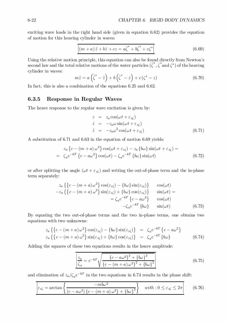
6-22 CHAPTER 6. RIGID BODY DYNAMICS
exciting wave loads in the right hand side (given in equation 6.62) provides the equationof motion for this heaving cylinder in waves:
¯¯(m + a) Äz + b _z + cz = aij¤ + b _³¤ + c³¤
¯¯ (6.69)
Using the relative motion principle, this equation can also be found directly from Newton’ssecond law and the total relative motions of the water particles (ij
¤, _³¤and ³¤) of the heaving
cylinder in waves:
mÄz = a³Ä³¤ ¡ Äz
´+ b
³_³¤ ¡ _z
´+ c (³¤ ¡ z) (6.70)
In fact, this is also a combination of the equations 6.25 and 6.62.
6.3.5 Response in Regular Waves
The heave response to the regular wave excitation is given by:
z = za cos(!t+ "z³ )
_z = ¡za! sin(!t+ "z³ )Äz = ¡za!2 cos(!t+ "z³ ) (6.71)
A substitution of 6.71 and 6.63 in the equation of motion 6.69 yields:
za©c¡ (m + a)!2
ªcos(!t+ "z³) ¡ za fb!g sin(!t + "z³ ) =
= ³ae¡kT ©
c¡ a!2ªcos(!t)¡ ³ae¡kT fb!g sin(!t) (6.72)
or after splitting the angle (!t+ "z³ ) and writing the out-of-phase term and the in-phaseterm separately:
za©©c ¡ (m+ a)!2
ªcos("z³) ¡ fb!g sin("z³)
ªcos(!t)
¡za©©c¡ (m+ a)!2
ªsin("z³) + fb!g cos("z³)
ªsin(!t) =
= ³ae¡kT ©
c¡ a!2ª
cos(!t)
¡³ae¡kT fb!g sin(!t) (6.73)
By equating the two out-of-phase terms and the two in-phase terms, one obtains twoequations with two unknowns:
za©©c ¡ (m+ a)!2
ªcos("z³) ¡ fb!g sin("z³)
ª= ³ae
¡kT ©c¡ a!2
ª
za©©c¡ (m+ a)!2
ªsin("z³ ) + fb!g cos("z³)
ª= ³ae
¡kT fb!g (6.74)
Adding the squares of these two equations results in the heave amplitude:¯¯¯za³a= e¡kT
sfc¡ a!2g2 + fb!g2
fc ¡ (m+ a)!2g2 + fb!g2
¯¯¯ (6.75)
and elimination of za=³ae¡kT in the two equations in 6.74 results in the phase shift:
¯¯"z³ = arctan
½ ¡mb!3(c¡ a!2) fc¡ (m+ a)!2g + fb!g2
¾with : 0 · "z³ · 2¼
¯¯ (6.76)
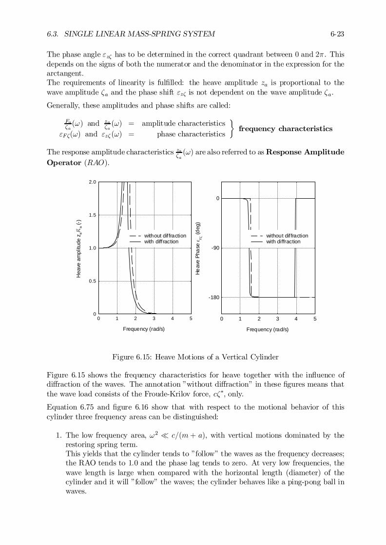
6.3. SINGLE LINEAR MASS-SPRING SYSTEM 6-23
The phase angle "z³ has to be determined in the correct quadrant between 0 and 2¼. Thisdepends on the signs of both the numerator and the denominator in the expression for thearctangent.The requirements of linearity is ful…lled: the heave amplitude za is proportional to thewave amplitude ³a and the phase shift "z³ is not dependent on the wave amplitude ³a.
Generally, these amplitudes and phase shifts are called:
Fa³a(!) and za
³a(!) = amplitude characteristics
"F³(!) and "z³ (!) = phase characteristics
¾frequency characteristics
The response amplitude characteristics za³a(!) are also referred to as Response Amplitude
Operator (RAO).
0
0.5
1.0
1.5
2.0
0 1 2 3 4 5
without diffractionwith diffraction
Frequency (rad/s)
Hea
ve a
mpl
itude
za/ζ
a (-
)
-180
-90
0
0 1 2 3 4 5
without diffractionwith diffraction
Frequency (rad/s)
He
ave
Pha
se ε
z ζ (d
eg)
Figure 6.15: Heave Motions of a Vertical Cylinder
Figure 6.15 shows the frequency characteristics for heave together with the in‡uence ofdi¤raction of the waves. The annotation ”without di¤raction” in these …gures means thatthe wave load consists of the Froude-Krilov force, c³¤, only.
Equation 6.75 and …gure 6.16 show that with respect to the motional behavior of thiscylinder three frequency areas can be distinguished:
1. The low frequency area, !2 ¿ c=(m+ a), with vertical motions dominated by therestoring spring term.This yields that the cylinder tends to ”follow” the waves as the frequency decreases;the RAO tends to 1.0 and the phase lag tends to zero. At very low frequencies, thewave length is large when compared with the horizontal length (diameter) of thecylinder and it will ”follow” the waves; the cylinder behaves like a ping-pong ball inwaves.
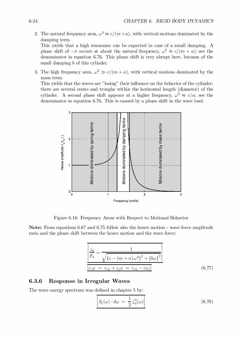
6-24 CHAPTER 6. RIGID BODY DYNAMICS
2. The natural frequency area, !2 t c=(m+a), with vertical motions dominated by thedamping term.This yields that a high resonance can be expected in case of a small damping. Aphase shift of ¡¼ occurs at about the natural frequency, !2 t c=(m + a); see thedenominator in equation 6.76. This phase shift is very abrupt here, because of thesmall damping b of this cylinder.
3. The high frequency area, !2 À c=(m+ a), with vertical motions dominated by themass term.This yields that the waves are ”losing” their in‡uence on the behavior of the cylinder;there are several crests and troughs within the horizontal length (diameter) of thecylinder. A second phase shift appears at a higher frequency, !2 t c=a; see thedenominator in equation 6.76. This is caused by a phase shift in the wave load.
Figure 6.16: Frequency Areas with Respect to Motional Behavior
Note: From equations 6.67 and 6.75 follow also the heave motion - wave force amplituderatio and the phase shift between the heave motion and the wave force:
¯¯¯zaFa=
1qfc¡ (m + a)!2g2 + fb!g2
¯¯¯
j"zF = "z³ + "³F = "z³ ¡ "F³j (6.77)
6.3.6 Response in Irregular Waves
The wave energy spectrum was de…ned in chapter 5 by:¯¯S³ (!) ¢ d! =
1
2³2a(!)
¯¯ (6.78)
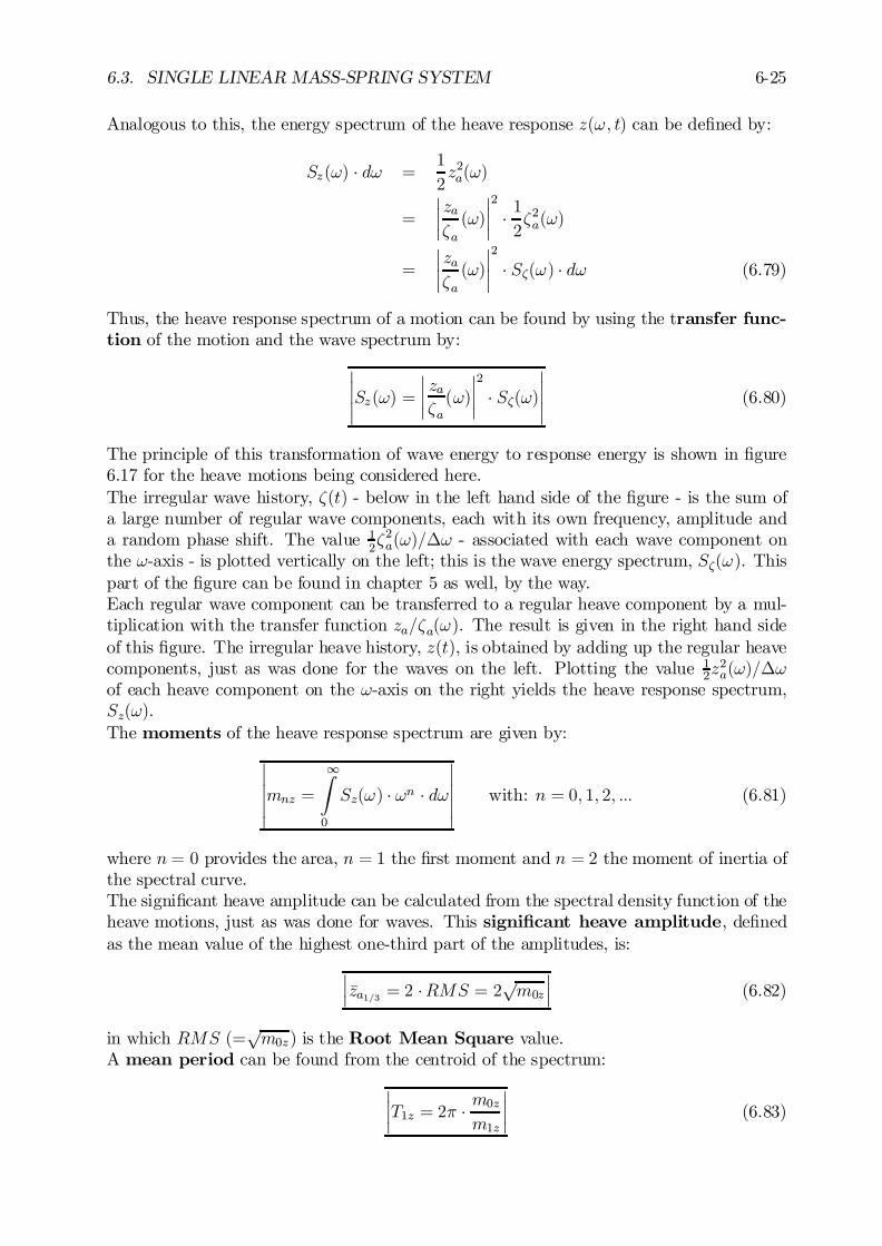
6.3. SINGLE LINEAR MASS-SPRING SYSTEM 6-25
Analogous to this, the energy spectrum of the heave response z(!; t) can be de…ned by:
Sz(!) ¢ d! =1
2z2a(!)
=
¯¯za³a(!)
¯¯2
¢ 12³2a(!)
=
¯¯za³a(!)
¯¯2
¢ S³(!) ¢ d! (6.79)
Thus, the heave response spectrum of a motion can be found by using the transfer func-tion of the motion and the wave spectrum by:
¯¯¯Sz(!) =
¯¯ za³a(!)
¯¯2
¢ S³(!)¯¯¯ (6.80)
The principle of this transformation of wave energy to response energy is shown in …gure6.17 for the heave motions being considered here.The irregular wave history, ³(t) - below in the left hand side of the …gure - is the sum ofa large number of regular wave components, each with its own frequency, amplitude anda random phase shift. The value 1
2³2a(!)=¢! - associated with each wave component on
the !-axis - is plotted vertically on the left; this is the wave energy spectrum, S³(!). Thispart of the …gure can be found in chapter 5 as well, by the way.Each regular wave component can be transferred to a regular heave component by a mul-tiplication with the transfer function za=³a(!). The result is given in the right hand sideof this …gure. The irregular heave history, z(t), is obtained by adding up the regular heavecomponents, just as was done for the waves on the left. Plotting the value 1
2z2a(!)=¢!
of each heave component on the !-axis on the right yields the heave response spectrum,Sz(!).The moments of the heave response spectrum are given by:
¯¯¯mnz =
1Z
0
Sz(!) ¢ !n ¢ d!
¯¯¯ with: n = 0; 1; 2; ::: (6.81)
where n = 0 provides the area, n = 1 the …rst moment and n = 2 the moment of inertia ofthe spectral curve.The signi…cant heave amplitude can be calculated from the spectral density function of theheave motions, just as was done for waves. This signi…cant heave amplitude, de…nedas the mean value of the highest one-third part of the amplitudes, is:
¯¯¹za1=3 = 2 ¢RMS = 2pm0z
¯¯ (6.82)
in which RMS (=pm0z) is the Root Mean Square value.
A mean period can be found from the centroid of the spectrum:
¯¯T1z = 2¼ ¢ m0z
m1z
¯¯ (6.83)
6-26 CHAPTER 6. RIGID BODY DYNAMICS
Figure 6.17: Principle of Transfer of Waves into Responses
Another de…nition, which is equivalent to the average zero-crossing period, is foundfrom the spectral radius of gyration:
¯¯T2z = 2¼ ¢
rm0zm2z
¯¯ (6.84)
6.3.7 Spectrum Axis Transformation
When wave spectra are given as a function of frequencies in Herz (f = 1=T ) and one needsthis on an !-basis (in radians/sec), they have to be transformed just as was done for wavesin chapter 5. The heave spectrum on this !-basis becomes:
Sz(!) =Sz(f)
2¼
=
¯¯za³a(f or !)
¯¯2
¢ S³(f )2¼
(6.85)
6.4. SECOND ORDER WAVE DRIFT FORCES 6-27
6.4 Second Order Wave Drift Forces
Now that the …rst order behavior of linear (both mechanical as well as hydromechanical)systems has been handled, attention in the rest of this chapter shifts to nonlinear systems.Obviously hydrodynamics will get the most emphasis in this section, too.The e¤ects of second order wave forces are most apparent in the behavior of anchoredor moored ‡oating structures. In contrast to what has been handled above, these arehorizontally restrained by some form of mooring system. Analyses of the horizontal motionsof moored or anchored ‡oating structures in a seaway show that the responses of thestructure on the irregular waves include three important components:
1. A mean displacement of the structure, resulting from a constant load component.Obvious sources of these loads are current and wind. In addition to these, there isalso a so-called mean wave drift force. This drift force is caused by non-linear(second order) wave potential e¤ects. Together with the mooring system, these loadsdetermine the new equilibrium position - possibly both a translation and (in‡uencedby the mooring system) a yaw angle - of the structure in the earth-bound coordinatesystem. This yaw is of importance for the determination of the wave attack angle.
2. An oscillating displacement of the structure at frequencies corresponding to those ofthe waves; the wave-frequency region.These are linear motions with a harmonic character, caused by the …rst order waveloads. The principle of this has been presented above for the vertically oscillatingcylinder. The time-averaged value of this wave load and the resulting motion com-ponent are zero.
3. An oscillating displacement of the structure at frequencies which are much lower thanthose of the irregular waves; the low-frequency region.These motions are caused by non-linear elements in the wave loads, the low-frequencywave drift forces, in combination with spring characteristics of the mooring system.Generally, a moored ship has a low natural frequency in its horizontal modes of mo-tion as well as very little damping at such frequencies. Very large motion amplitudescan then result at resonance so that a major part of the ship’s dynamic displacement(and resulting loads in the mooring system) can be caused by these low-frequencyexcitations.
Item 2 of this list has been discussed in earlier parts of this chapter; the discussion of item1 starts below; item 3 is picked up later in this chapter and along with item 1 again inchapter 9.
6.4.1 Mean Wave Loads on a Wall
Mean wave loads in regular waves on a wall can be calculated simply from the pressure in the‡uid, now using the more complete (not-linearized!) Bernoulli equation. The superpositionprinciple can still be used to determine these loads in irregular waves. When the waves arenot too long, this procedure can be used, too, to estimate the mean wave drift forces on aship in beam waves (waves approaching from the side of the ship).

6-28 CHAPTER 6. RIGID BODY DYNAMICS
Regular Waves
A regular wave (in deep water) hits a vertical wall with an in…nite depth as shown in …gure6.18. This wave will be re‡ected fully, so that a standing wave (as described in chapter 5)results at the wall.
Figure 6.18: Regular Wave at a Wall
The incident undisturbed wave is de…ned by:¯¯©i = ¡³ag
!¢ ekz ¢ sin(+kx+ !t)
¯¯ and j³i = ³a ¢ cos(+kx +!t)j (6.86)
and the re‡ected wave by:¯¯©r = ¡³ag
!¢ ekz ¢ sin(¡kx+ !t)
¯¯ and j³r = ³a ¢ cos(¡kx +!t)j (6.87)
Then the total wave system can be determined by a superposition of these two waves; thisresults in a standing wave system:
© = ©i + ©r = ¡2 ¢ ³ag!
¢ ekz ¢ cos(kx) ¢ sin(!t)³ = ³i + ³r = 2 ¢ ³a ¢ cos(kx) ¢ cos(!t) (6.88)
The pressure in the ‡uid follows from the complete Bernoulli equation:
p = ¡½g ¢ z ¡ ½ ¢ @©@t
¡ 1
2½ ¢ (r©)2
= ¡½g ¢ z ¡ ½ ¢ @©@t
¡ 1
2½ ¢
(µ@©
@x
¶2
+
µ@©
@z
¶2)(6.89)
The derivatives of the potential ©(x; z; t) with respect to t, x and z are given by:
@©
@t= ¡2 ¢ ³a ¢ g ¢ ekz ¢ cos(kx) ¢ cos(!t)
u =@©
@x= +2 ¢ ³a ¢ ! ¢ ekz ¢ sin(kx) ¢ sin(!t)
w =@©
@z= ¡2 ¢ ³a ¢ ! ¢ ekz ¢ cos(kx) ¢ sin(!t) (6.90)

6.4. SECOND ORDER WAVE DRIFT FORCES 6-29
At the wall (x = 0), the wave elevation and the derivatives of the potential are:
³ = 2 ¢ ³a ¢ cos(!t)@©
@t= ¡2 ¢ ³a ¢ g ¢ ekz ¢ cos(!t)
u =@©
@x= 0
w =@©
@z= ¡2 ¢ ³a ¢ ! ¢ ekz ¢ sin(!t) (6.91)
and the pressure on the wall is:
p = ¡½g ¢ z ¡ ½ ¢ @©@t
¡ 1
2½ ¢
(µ@©
@x
¶2
+
µ@©
@z
¶2)
= ¡½g ¢ z + 2½g ¢ ³a ¢ ekz ¢ cos(!t) ¡ 1
2½ ¢
¡4³a
2 ¢ !2 ¢ e2kz sin2(!t)¢
= ¡½g ¢ z + 2½g ¢ ³a ¢ ekz ¢ cos(!t) ¡ ½ ¢ ³a2 ¢ !2 ¢ e2kz ¢ (1 ¡ cos(2!t)) (6.92)
This time-varying pressure on the wall can also be written as:
p = ¹p(0)+ ~p(1)+ ¹p(2) + ~p(2) (6.93)
where:
¹p(0) = ¡½g ¢ z~p(1) = +2½g ¢ ³a ¢ ekz ¢ cos(!t)¹p(2) = ¡½ ¢ ³a2 ¢ !2 ¢ e2kz~p(2) = +½ ¢ ³a2 ¢ !2 ¢ e2kz ¢ cos(2!t) (6.94)
The general expression for the mean force on the wall follows from:
F = ¡³Z
¡1
(¹p ¢ ¹n) ¢ dS (6.95)
where the superscript bar over the entire integral indicates a (long) time average.Because ¹n = (1; 0; 0) and dS = 1 ¢ dz, this mean force becomes:
¹F = ¡³(t)Z
¡1
p(z; t) ¢ dz (6.96)
which is split into two parts over the vertical axis; one above and one below the still waterlevel:
¹F = ¡0Z
¡1
p(z; t) ¢ dz ¡³(t)Z
0
p(z; t) ¢ dz (6.97)
= F1 + F2 (6.98)
6-30 CHAPTER 6. RIGID BODY DYNAMICS
where:p(z; t) = ¹p(0) + ~p(1)+ ¹p(2)+ ~p(2) and ³(t) = ~³
(1)(t) (6.99)
The …rst part F1 comes from the integration from ¡1 to 0; it contributes to the integrationof ¹p(0) and ¹p(2) only:
F1 = ¡0Z
¡1
p(z; t) ¢ dz
= ¡0Z
¡1
¡¡½gz ¡ ½ ¢ ³a2 ¢!2 ¢ e2kz
¢¢ dz
= ½ ¢ !2 ¢ ³a20Z
¡1
e2kz ¢ dz
= +1
2½g ¢ ³a2 (6.100)
This force is directed away from the wall. The static …rst term (¡½gz) has been left outof consideration, while the dispersion relation for deep water (!2 = kg) has been utilizedin the second term.The second part, F2, comes from the integration from 0 to ³(t); it contributes to theintegration of ¹p(0) and ~p(1) only, so that the time-dependent force F2(t) becomes:
F2(t) = ¡³(t)Z
0
p(z; t) ¢ dz
= ¡³(t)Z
0
(¡½g ¢ z + ½g ¢ ³(t)) ¢ dz
= +½g
³(t)Z
0
z ¢ dz ¡ ½g³(t)Z
0
³(t) ¢ dz
= +1
2½g ¢ f³(t)g2 ¡ ½g ¢ f³(t)g2
= ¡12½g ¢ f³(t)g2 (6.101)
Because
³(t) = 2 ¢ ³a ¢ cos(!t) and cos2(!t) =1
2¢ (1 + cos(2!t)) (6.102)
this part of the force becomes:
F2(t) = ¡12½g ¢ 4 ¢ ³a2 ¢ cos2(!t)
= ¡½g ¢ ³a2 ¢ (1 + cos(2!t)) (6.103)

6.4. SECOND ORDER WAVE DRIFT FORCES 6-31
Figure 6.19: Mean Wave Loads on a Wall
The desired time-averaged value becomes:
F2 = ¡½g ¢ ³a2 (6.104)
where ³a is the amplitude of the incoming wave. This force is directed toward the wall.Finally, see …gure 6.19, the total time-averaged force ¹F per meter length of the wall be-comes:
¹F = F1 + F2
= +1
2½g ¢ ³a2 ¡ ½g ¢ ³a2 (6.105)
Thus: ¯¯ ¹F = ¡1
2½g ¢ ³a2
¯¯ (6.106)
in which it is assumed that the incident wave is fully re‡ected. This total force has amagnitude proportional to the square of the incoming wave amplitude and it is directedtoward the wall.Note that this force is also directly related to the energy per unit area of the incomingwaves as found in chapter 5:
E =1
2½g ¢ ³2a (6.107)
Comparison of equations 6.106 and 6.107 reveals that the mean wave drift force is numer-ically equal to the energy per unit area of the incoming waves.
Irregular Waves
The discovery just made above will be utilized to determine the mean wave drift force fromirregular waves as well. This is done via the wave spectrum, de…ned by:
S³(!) ¢ d! =1
2³a2(!) with a zero order moment: m0 =
1Z
0
S³ (!) ¢ d! (6.108)
Then the total force on the wall can be written as:
¹F = ¡X 1
2½g ¢ ³a2(!)
6-32 CHAPTER 6. RIGID BODY DYNAMICS
= ¡½g1Z
0
S³(!) ¢ d!
= ¡½g ¢m0³ (6.109)
Because:
H1=3 = 4pm0³ or m0³ =
1
16¢H1=3
2 (6.110)
it follows that the mean wave drift force can be expressed as:¯¯ ¹F = ¡1
16¢ ½g ¢H1=3
2
¯¯ per metre length of the wall (6.111)
Approximation for Ships
It has been assumed so far that the incident wave is fully re‡ected. When the waves are nottoo long, so that the water motion is more or less concentrated near the sea surface (overthe draft of the ship), full re‡ection can be assumed for large ships too. Then, equation6.111 can be used for a …rst estimation of the mean wave drift forces on a ship in beamwaves.The mean wave drift force on an example ship with a length L of 300 meters in beam waveswith a signi…cant wave height H 1=3 of 4.0 meters can be approximated easily. Assumingthat all waves will be re‡ected, the mean wave drift force is:
¹F =1
16¢ ½g ¢H1=3
2 ¢ L
=1
16¢ 1:025 ¢ 9:806 ¢ 4:02 ¢ 300 ¼ 3000 kN (6.112)
6.4.2 Mean Wave Drift Forces
[Maruo, 1960] showed for the two-dimensional case of an in…nitely long cylinder ‡oating inregular waves with its axis perpendicular to the wave direction that the mean wave driftforce per unit length satis…es: ¯
¯ ¹F 0 =1
2½g ¢ ³ar2
¯¯ (6.113)
in which ³ar is the amplitude of the wave re‡ected and scattered by the body in a directionopposite to the incident wave.Generally only a part of the incident regular wave will be re‡ected; the rest will be trans-mitted underneath the ‡oating body. Besides the re‡ected wave, additional waves aregenerated by the heave, pitch and roll motions of the vessel. The re‡ected and scatteredwaves have the same frequency as the incoming wave, so that the sum of these compo-nents still has the same frequency as the incoming wave. Their amplitudes will depend onthe amplitudes and relative phases of the re‡ected and scattered wave components. Theamplitudes of these components and their phase di¤erences depend on the frequency ofthe incident wave, while the amplitudes can be assumed to be linearly proportional to theamplitude of the incident wave. This is because it is the incident wave amplitude whichcauses the body to move in the …rst place. In equation form:
³ar = R(!) ¢ ³a (6.114)
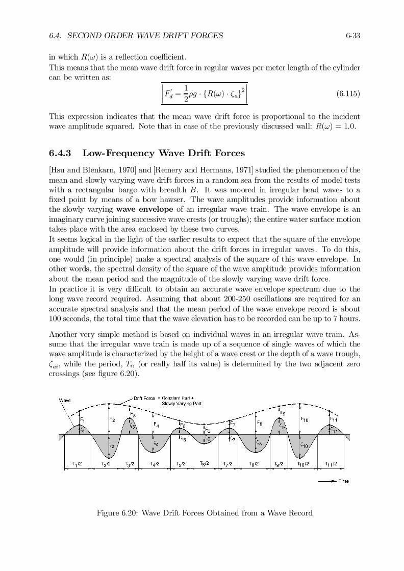
6.4. SECOND ORDER WAVE DRIFT FORCES 6-33
in which R(!) is a re‡ection coe¢cient.This means that the mean wave drift force in regular waves per meter length of the cylindercan be written as: ¯
¯F 0d =
1
2½g ¢ fR(!) ¢ ³ag2
¯¯ (6.115)
This expression indicates that the mean wave drift force is proportional to the incidentwave amplitude squared. Note that in case of the previously discussed wall: R(!) = 1:0.
6.4.3 Low-Frequency Wave Drift Forces
[Hsu and Blenkarn, 1970] and [Remery and Hermans, 1971] studied the phenomenon of themean and slowly varying wave drift forces in a random sea from the results of model testswith a rectangular barge with breadth B. It was moored in irregular head waves to a…xed point by means of a bow hawser. The wave amplitudes provide information aboutthe slowly varying wave envelope of an irregular wave train. The wave envelope is animaginary curve joining successive wave crests (or troughs); the entire water surface motiontakes place with the area enclosed by these two curves.It seems logical in the light of the earlier results to expect that the square of the envelopeamplitude will provide information about the drift forces in irregular waves. To do this,one would (in principle) make a spectral analysis of the square of this wave envelope. Inother words, the spectral density of the square of the wave amplitude provides informationabout the mean period and the magnitude of the slowly varying wave drift force.In practice it is very di¢cult to obtain an accurate wave envelope spectrum due to thelong wave record required. Assuming that about 200-250 oscillations are required for anaccurate spectral analysis and that the mean period of the wave envelope record is about100 seconds, the total time that the wave elevation has to be recorded can be up to 7 hours.
Another very simple method is based on individual waves in an irregular wave train. As-sume that the irregular wave train is made up of a sequence of single waves of which thewave amplitude is characterized by the height of a wave crest or the depth of a wave trough,³ai, while the period, Ti, (or really half its value) is determined by the two adjacent zerocrossings (see …gure 6.20).
Figure 6.20: Wave Drift Forces Obtained from a Wave Record
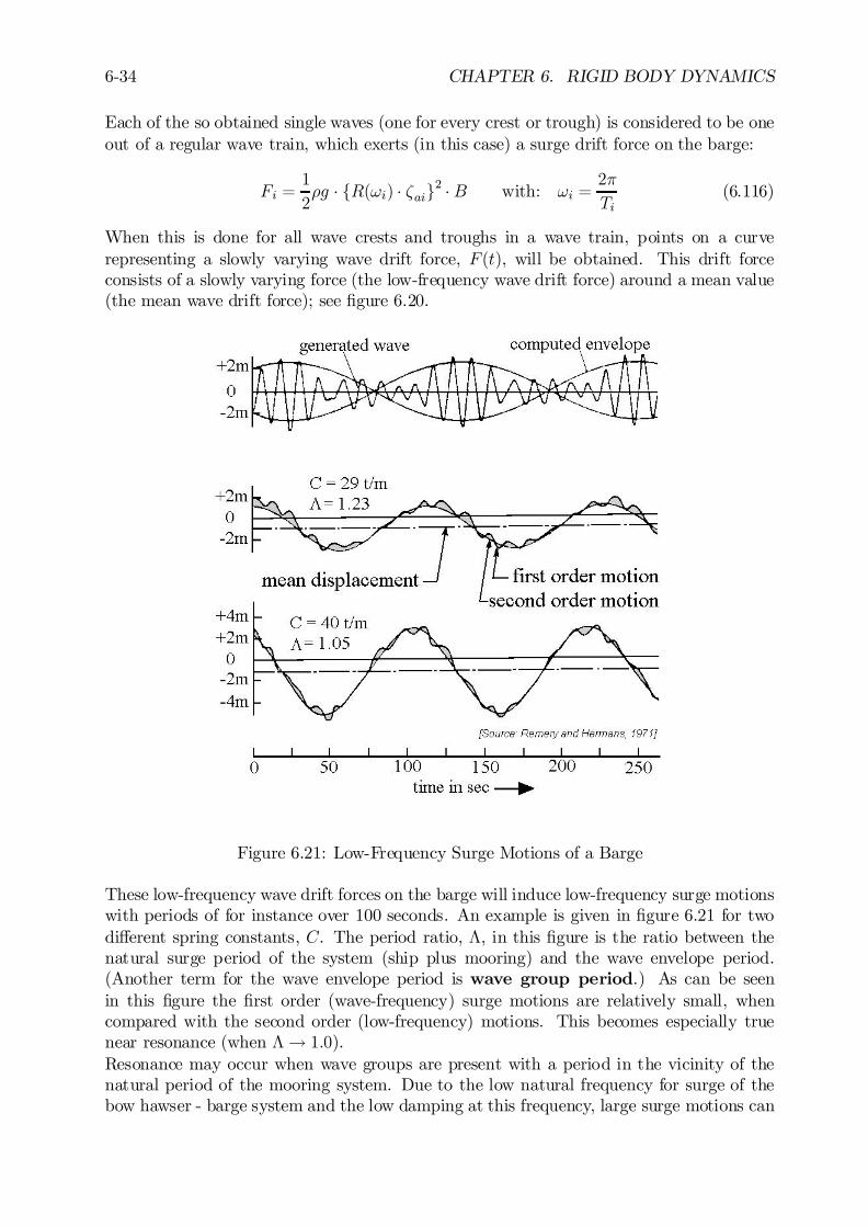
6-34 CHAPTER 6. RIGID BODY DYNAMICS
Each of the so obtained single waves (one for every crest or trough) is considered to be oneout of a regular wave train, which exerts (in this case) a surge drift force on the barge:
Fi =1
2½g ¢ fR(!i) ¢ ³aig2 ¢B with: !i =
2¼
Ti(6.116)
When this is done for all wave crests and troughs in a wave train, points on a curverepresenting a slowly varying wave drift force, F (t), will be obtained. This drift forceconsists of a slowly varying force (the low-frequency wave drift force) around a mean value(the mean wave drift force); see …gure 6.20.
Figure 6.21: Low-Frequency Surge Motions of a Barge
These low-frequency wave drift forces on the barge will induce low-frequency surge motionswith periods of for instance over 100 seconds. An example is given in …gure 6.21 for twodi¤erent spring constants, C. The period ratio, ¤, in this …gure is the ratio between thenatural surge period of the system (ship plus mooring) and the wave envelope period.(Another term for the wave envelope period is wave group period.) As can be seenin this …gure the …rst order (wave-frequency) surge motions are relatively small, whencompared with the second order (low-frequency) motions. This becomes especially truenear resonance (when ¤! 1:0).Resonance may occur when wave groups are present with a period in the vicinity of thenatural period of the mooring system. Due to the low natural frequency for surge of thebow hawser - barge system and the low damping at this frequency, large surge motions can
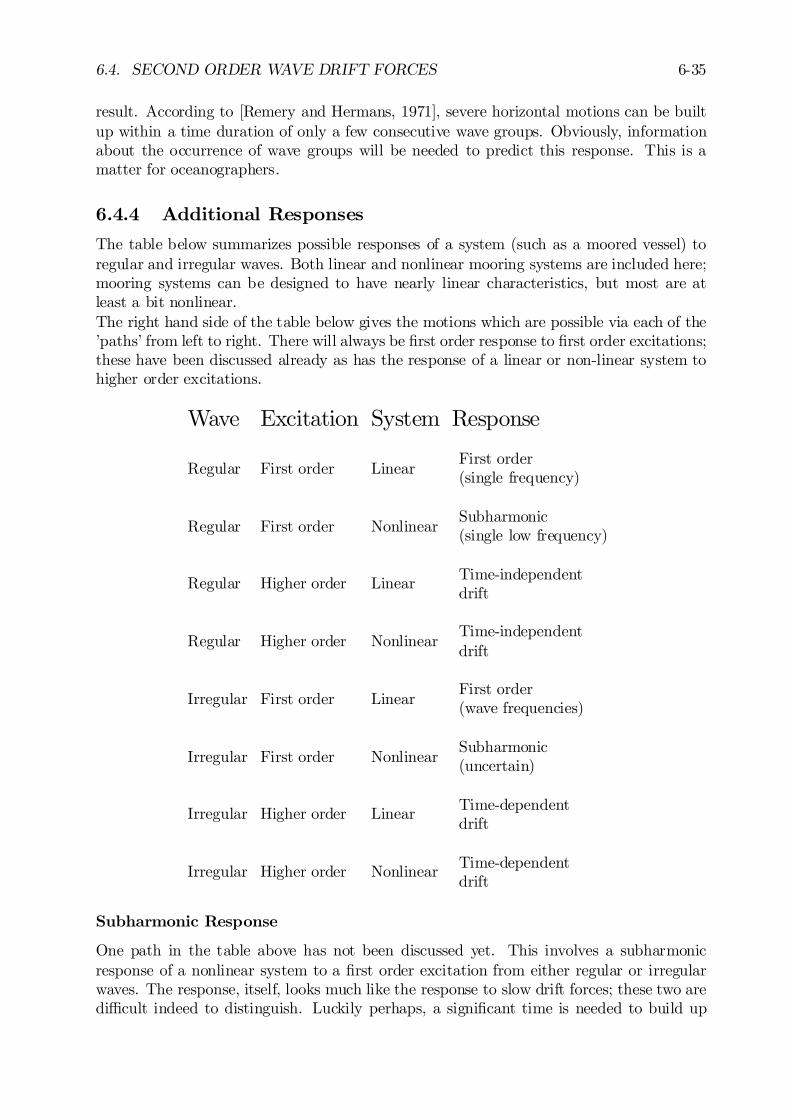
6.4. SECOND ORDER WAVE DRIFT FORCES 6-35
result. According to [Remery and Hermans, 1971], severe horizontal motions can be builtup within a time duration of only a few consecutive wave groups. Obviously, informationabout the occurrence of wave groups will be needed to predict this response. This is amatter for oceanographers.
6.4.4 Additional Responses
The table below summarizes possible responses of a system (such as a moored vessel) toregular and irregular waves. Both linear and nonlinear mooring systems are included here;mooring systems can be designed to have nearly linear characteristics, but most are atleast a bit nonlinear.The right hand side of the table below gives the motions which are possible via each of the’paths’ from left to right. There will always be …rst order response to …rst order excitations;these have been discussed already as has the response of a linear or non-linear system tohigher order excitations.
Wave Excitation System Response
Regular First order LinearFirst order(single frequency)
Regular First order NonlinearSubharmonic(single low frequency)
Regular Higher order Linear Time-independentdrift
Regular Higher order NonlinearTime-independentdrift
Irregular First order LinearFirst order(wave frequencies)
Irregular First order NonlinearSubharmonic(uncertain)
Irregular Higher order Linear Time-dependentdrift
Irregular Higher order Nonlinear Time-dependentdrift
Subharmonic Response
One path in the table above has not been discussed yet. This involves a subharmonicresponse of a nonlinear system to a …rst order excitation from either regular or irregularwaves. The response, itself, looks much like the response to slow drift forces; these two aredi¢cult indeed to distinguish. Luckily perhaps, a signi…cant time is needed to build up
6-36 CHAPTER 6. RIGID BODY DYNAMICS
subharmonic resonant motions of high amplitude. This implies that the excitation mustremain very nicely behaved over quite some time in order for this to happen. Waves at seaare very often too irregular; this subharmonic motion breaks down before large amplitudesare generated.
6.5 Time Domain Approach
If (as has been assumed so far in most of this chapter) the system is linear, such that itsbehavior is linearly related to its displacement, velocity and acceleration, then the behaviorof the system can be studied in the frequency domain.However, in a lot of cases there are several complications which violate this linear assump-tion, for instance nonlinear viscous damping, forces and moments due to currents, wind,anchoring and not to mention second order wave loads. If the system is nonlinear, thensuperposition principle - the foundation of the frequency domain approach - is no longervalid. Instead, one is forced to revert to the direct solution of the equations of motion asfunctions of time. These equations of motion result directly from Newton’s second law.Approaches to their solution are presented in this section.
6.5.1 Impulse Response Functions
The hydromechanical reaction forces and moments, due to time varying ship motions,can be described using the classic formulation given by [Cummins, 1962]. Complex po-tential problems, can be handled via frequency-dependent potential coe¢cients as done by[Ogilvie, 1964]. The principle of this approach will be demonstrated here for a motion withone degree of freedom. Insight about the possibilities of this method is more important inthis section than the details of the derivations involved; the result is more important thanthe exact route leading to it.
Cummins Equation
The ‡oating object is assumed to be a linear system with a translational (or rotational)velocity as input and the reaction force (or moment) of the surrounding water as output.The object is assumed to be at rest at time t = t0.During a short time interval, ¢t, the body experiences an impulsive displacement, ¢x,with a constant velocity, V , so that:
¢x = V ¢¢t (6.117)
During this impulsive displacement, the water particles will start to move. Since potential‡ow is assumed, a velocity potential, ©, proportional to the velocity, V , can be de…ned:
©(x; y; z; t) = ª(x; y; z) ¢ V (t) for: t0 < t < t0 +¢t (6.118)
in which ª is the normalized velocity potential.Note: This ª is not a stream function as used in chapter 3; this notation is used here toremain consistent with other literature.
6.5. TIME DOMAIN APPROACH 6-37
The water particles are still moving after this impulsive displacement, ¢x. Because thesystem is assumed to be linear, the motions of the ‡uid, described by the velocity potential,©, are proportional to the impulsive displacement, ¢x. So:
©(x; y; z; t) = Â(x; y; z; t) ¢¢x for: t > t0 + ¢t (6.119)
in which  is another normalized velocity potential.A general conclusion can be that the impulsive displacement, ¢x, during the time interval(t0; t0 + ¢t) in‡uences the motions of the ‡uid during this interval as well as during alllater time intervals. Similarly, the motions during the interval (t0; t0 +¢t) are in‡uencedby the motions before this interval; the system has a form of ”memory”.When the object performs an arbitrarily time-dependent varying motion, this motion canbe considered to be a succession of small impulsive displacements, so that then the resultingtotal velocity potential, ©(t), during the interval (tm; tm +¢t) becomes:
©(t) = Vm ¢ª +mX
k=1
fÂ(tm¡k; tm¡k +¢t) ¢ Vk ¢¢tg (6.120)
with:m = number of time steps (-)tm = t0 +m ¢¢t (s)tm¡k = t0 + (m¡ k) ¢¢t (s)Vm = velocity component during time interval (tm; tm + ¢t) (m/s)Vk = velocity component during time interval (tm¡k; tm¡k + ¢t) (m/s)ª = normalized velocity potential caused by a displacement
during time interval (tm; tm + ¢t)Â = normalized velocity potential caused by a displacement
during time interval (tm¡k; tm¡k + ¢t)
Letting ¢t go to zero, yields:
©(t) = _x(t) ¢ª+tZ
¡1
Â(t¡ ¿) ¢ _x(¿) ¢ d¿ (6.121)
in which _x(¿) is the velocity component of the body at time ¿ .The pressure in the ‡uid follows from the linearized Bernoulli equation:
p = ¡½ ¢ @©@t
(6.122)
An integration of these pressures over the wetted surface, S , of the ‡oating object yieldsthe expression for the hydrodynamic reaction force (or moment), F .With n is the generalized directional cosine in a vector notation, F becomes:
F = ¡Z Z
S
p ¢ n ¢ dS
=
8<:½
Z Z
S
ª ¢ n ¢ dS
9=; ¢ Äx(t)
+
tZ
¡1
8<:½
Z Z
S
@Â(t¡ ¿ )@t
¢ n ¢ dS
9=; ¢ _x(¿) ¢ d¿ (6.123)
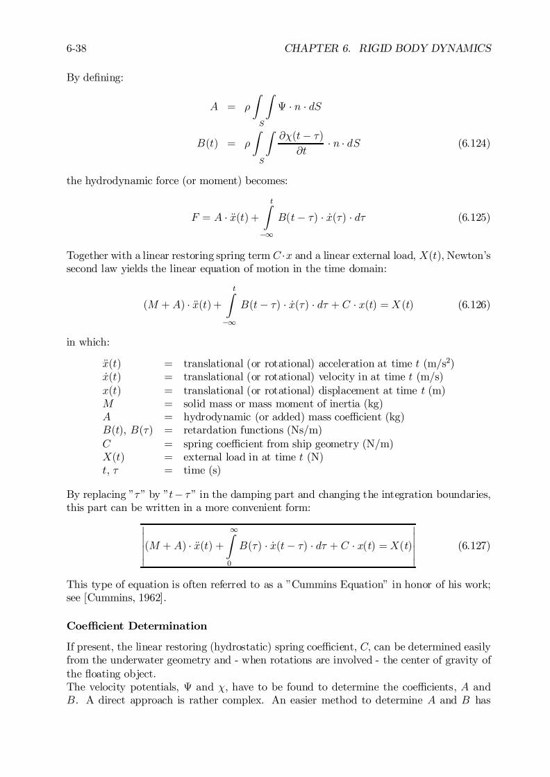
6-38 CHAPTER 6. RIGID BODY DYNAMICS
By de…ning:
A = ½
Z Z
S
ª ¢ n ¢ dS
B(t) = ½
Z Z
S
@Â(t¡ ¿)@t
¢ n ¢ dS (6.124)
the hydrodynamic force (or moment) becomes:
F = A ¢ Äx(t) +tZ
¡1
B(t¡ ¿) ¢ _x(¿) ¢ d¿ (6.125)
Together with a linear restoring spring term C ¢x and a linear external load, X(t), Newton’ssecond law yields the linear equation of motion in the time domain:
(M + A) ¢ Äx(t) +tZ
¡1
B(t¡ ¿) ¢ _x(¿) ¢ d¿ + C ¢ x(t) =X (t) (6.126)
in which:
Äx(t) = translational (or rotational) acceleration at time t (m/s2)_x(t) = translational (or rotational) velocity in at time t (m/s)x(t) = translational (or rotational) displacement at time t (m)M = solid mass or mass moment of inertia (kg)A = hydrodynamic (or added) mass coe¢cient (kg)B(t), B(¿) = retardation functions (Ns/m)C = spring coe¢cient from ship geometry (N/m)X(t) = external load in at time t (N)t, ¿ = time (s)
By replacing ”¿” by ”t¡ ¿” in the damping part and changing the integration boundaries,this part can be written in a more convenient form:
¯¯¯(M + A) ¢ Äx(t) +
1Z
0
B(¿) ¢ _x(t¡ ¿) ¢ d¿ + C ¢ x(t) =X(t)
¯¯¯ (6.127)
This type of equation is often referred to as a ”Cummins Equation” in honor of his work;see [Cummins, 1962].
Coe¢cient Determination
If present, the linear restoring (hydrostatic) spring coe¢cient, C; can be determined easilyfrom the underwater geometry and - when rotations are involved - the center of gravity ofthe ‡oating object.The velocity potentials, ª and Â, have to be found to determine the coe¢cients, A andB. A direct approach is rather complex. An easier method to determine A and B has
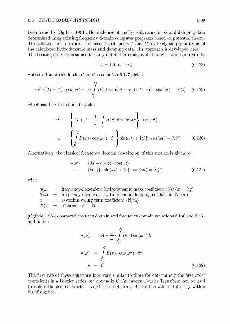
6.5. TIME DOMAIN APPROACH 6-39
been found by [Ogilvie, 1964]. He made use of the hydrodynamic mass and damping datadetermined using existing frequency domain computer programs based on potential theory.This allowed him to express the needed coe¢cients A and B relatively simply in terms ofthe calculated hydrodynamic mass and damping data. His approach is developed here.The ‡oating object is assumed to carry out an harmonic oscillation with a unit amplitude:
x = 1:0 ¢ cos(!t) (6.128)
Substitution of this in the Cummins equation 6.127 yields:
¡!2 ¢ (M +A) ¢ cos(!t)¡ ! ¢1Z
0
B(¿ ) ¢ sin(!t¡ !¿ ) ¢ d¿ +C ¢ cos(!t) = X(t) (6.129)
which can be worked out to yield:
¡!2¢
8<:M + A¡ 1
!¢1Z
0
B(¿ ) sin(!¿)d¿
9=; ¢ cos(!t)
¡!¢
8<:
1Z
0
B(¿ ) ¢ cos(!¿ ) ¢ d¿
9=; sin(!t) + fCg ¢ cos(!t) = X(t) (6.130)
Alternatively, the classical frequency domain description of this motion is given by:
¡!2¢ fM + a(!)g ¢ cos(!t)¡!¢ fb(!)g ¢ sin(!t) + fcg ¢ cos(!t) = X(t) (6.131)
with:
a(!) = frequency-dependent hydrodynamic mass coe¢cient (Ns2/m = kg)b(!) = frequency-dependent hydrodynamic damping coe¢cient (Ns/m)c = restoring spring term coe¢cient (N/m)X(t) = external force (N)
[Ogilvie, 1964] compared the time domain and frequency domain equations 6.130 and 6.131and found:
a(!) = A¡ 1
!¢1Z
0
B(¿) sin(!¿ )d¿
b(!) =
1Z
0
B(¿ ) ¢ cos(!¿) ¢ d¿
c = C (6.132)
The …rst two of these equations look very similar to those for determining the …rst ordercoe¢cients in a Fourier series; see appendix C. An inverse Fourier Transform can be usedto isolate the desired function, B(¿); the coe¢cient, A, can be evaluated directly with abit of algebra.
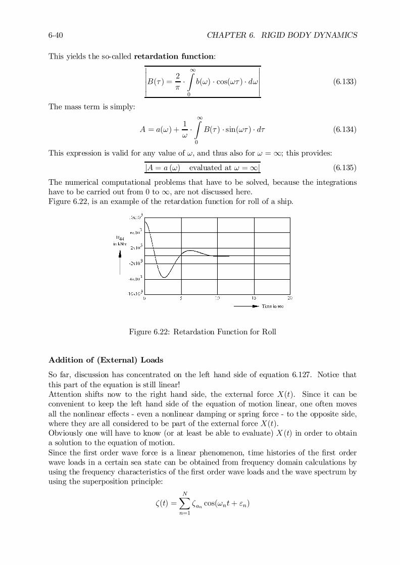
6-40 CHAPTER 6. RIGID BODY DYNAMICS
This yields the so-called retardation function:¯¯¯B(¿ ) =
2
¼¢1Z
0
b(!) ¢ cos(!¿ ) ¢ d!
¯¯¯ (6.133)
The mass term is simply:
A = a(!) +1
!¢1Z
0
B(¿ ) ¢ sin(!¿ ) ¢ d¿ (6.134)
This expression is valid for any value of !, and thus also for ! = 1; this provides:
jA = a (!) evaluated at ! =1j (6.135)
The numerical computational problems that have to be solved, because the integrationshave to be carried out from 0 to 1, are not discussed here.Figure 6.22, is an example of the retardation function for roll of a ship.
Figure 6.22: Retardation Function for Roll
Addition of (External) Loads
So far, discussion has concentrated on the left hand side of equation 6.127. Notice thatthis part of the equation is still linear!Attention shifts now to the right hand side, the external force X(t). Since it can beconvenient to keep the left hand side of the equation of motion linear, one often movesall the nonlinear e¤ects - even a nonlinear damping or spring force - to the opposite side,where they are all considered to be part of the external force X(t).Obviously one will have to know (or at least be able to evaluate) X (t) in order to obtaina solution to the equation of motion.Since the …rst order wave force is a linear phenomenon, time histories of the …rst orderwave loads in a certain sea state can be obtained from frequency domain calculations byusing the frequency characteristics of the …rst order wave loads and the wave spectrum byusing the superposition principle:
³(t) =NX
n=1
³an cos(!nt+ "n)

6.5. TIME DOMAIN APPROACH 6-41
with randomly chosen phase shifts, "n, between 0 and 2¼ and:
³an =q2 ¢ S³(!n) ¢¢! which follows from:
1
2³2an = S³(!n) ¢¢!
see chapter 5.With this, the time history of the …rst order wave load then becomes:
¯¯¯Xw(t) =
NX
n=1
µXwan³an
¶¢ ³an cos(!nt+ "n + "Xw³n)
¯¯¯ (6.136)
in which:
Xw(t) = wave load (N)N = number of frequencies (-)!n = wave frequency rad/s)Xwan³an
= transfer function of wave load (N/m)
"Xw³n = phase shift of wave load (rad)"n = phase shift of wave (rad)
Note that with a constant frequency interval , ¢!, this time history repeats itself after2¼=¢! seconds.With known coe¢cients and the right hand side of this equation of motion, equation 6.127can be integrated a numerically. Comparisons of calculated and transformed linear motionsin the frequency domain with time domain results show a perfect agreement.
Validation Tests
A series of simple model experiments have been carried out to validate the time domaincalculation routines with non-linear terms. Towing tank number 2 of the Delft Ship Hydro-mechanics Laboratory with a 1:40 model of the Oil Skimming Vessel m.v. Smal Agt (51.00x 9.05 x 3.25 meter) was used for this. Horizontal impulse forces in the longitudinal andlateral direction have been introduced in a tow line between a torque-motor and the modelin still water. The measured motions of the ship model have been compared with the datacalculated in the time domain, using the measured time-series of the impulse forces andassumed points of application as an input. An example of the comparison is presented in…gure 6.23 for the sway velocities due to a lateral impulse force amidships.The …gure shows a good agreement between the calculated and the measured sway motions.Comparable agreements have been found for the other tests.A few years ago, the Centre for Applied Research in The Netherlands (TNO) carried out aseries of full scale collision tests with two inland waterway tankers in still water, see …gure6.24. The contact forces between the two ships and the motions of the rammed ship (80.00x 8.15 x 2.20 meter) were measured. Computer simulations of the motion behavior of therammed ship during the collision have been carried out, using the measured contact forceson the rammed ship as an input.Figure 6.25 shows some comparative results for a test with a collision of the rammed shipat about 0.40 Lpp from the bow on the port side. The ramming ship had a speed of about15 km/hr. The measured and calculated motions of the rammed ship are presented. Sway,roll and yaw velocities are predicted here very well.
6-42 CHAPTER 6. RIGID BODY DYNAMICS
Figure 6.23: External Impulse and Resulting Motions
Figure 6.24: Underwater Portion of Rammed Ship
6.5.2 Direct Time Domain Simulation
Retardation functions as described above can be used to solve the equations of motionfor cases in which the nonlinearities can be included in the time-dependent excitation onthe right hand side of the equation. While it is possible to ”move” some nonlinearities tothe excitation side of the equation of motion more or less arti…cially, there are still manyrelevant physical systems which do not lend themselves to such a treatment.One example of such a system will come up at the end of chapter 12 when the hydrodynamicdrag on a moving cylinder in waves will be discussed. A perhaps more spectacular exampleinvolves the launching of an o¤shore tower structure from a barge. It should be obviousthat the hydrodynamic mass and damping of such a structure - and of the barge fromwhich it is launched - will change quite rapidly as the tower enters the water and load istransferred from the barge. Notice, now, that the hydromechanical coe¢cients - for boththe tower and barge - can best be expressed as (nonlinear) functions of the position of therespective structures rather than of time. These functions can easily be accommodated ina time domain calculation in which all conditions can be re-evaluated at the start of eachtime step.
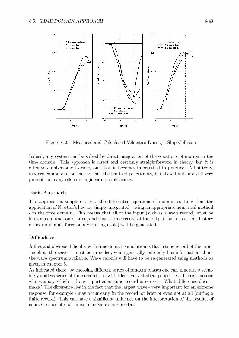
6.5. TIME DOMAIN APPROACH 6-43
Figure 6.25: Measured and Calculated Velocities During a Ship Collision
Indeed, any system can be solved by direct integration of the equations of motion in thetime domain. This approach is direct and certainly straightforward in theory, but it isoften so cumbersome to carry out that it becomes impractical in practice. Admittedly,modern computers continue to shift the limits of practicality, but these limits are still verypresent for many o¤shore engineering applications.
Basic Approach
The approach is simple enough: the di¤erential equations of motion resulting from theapplication of Newton’s law are simply integrated - using an appropriate numerical method- in the time domain. This means that all of the input (such as a wave record) must beknown as a function of time, and that a time record of the output (such as a time historyof hydrodynamic force on a vibrating cable) will be generated.
Di¢culties
A …rst and obvious di¢culty with time domain simulation is that a time record of the input- such as the waves - must be provided, while generally, one only has information aboutthe wave spectrum available. Wave records will have to be re-generated using methods asgiven in chapter 5.As indicated there, by choosing di¤erent series of random phases one can generate a seem-ingly endless series of time records, all with identical statistical properties. There is no-onewho can say which - if any - particular time record is correct. What di¤erence does itmake? The di¤erence lies in the fact that the largest wave - very important for an extremeresponse, for example - may occur early in the record, or later or even not at all (during a…nite record). This can have a signi…cant in‡uence on the interpretation of the results, ofcourse - especially when extreme values are needed.

6-44 CHAPTER 6. RIGID BODY DYNAMICS
The interpretation of time domain simulation results forms a second di¢culty in practice.A designer often needs a ”design response” (an extreme dynamic internal load or displace-ment) with an associated (small) probability that it will be exceeded as ”output” froma dynamic analysis. This interpretation di¢culty is brought into focus by reviewing theprocess for a linear system, …rst.One will generally analyze a linear system in the frequency domain; spectra of the desiredresponse are generated directly. Since the response spectra will be of essentially the sameform as the input spectra, the output can be transformed to convenient statistical data fordistributions interpretation - just as is done for waves. Once this theoretical distributionhas been …tted, it is a simple matter to extrapolate this to get the value associated withthe chosen design probability.When time domain simulation is used instead, one must …rst convert the generated timerecord of the output to some form of spectrum. If the system being analyzed is nonlinear,then the spectrum of the output need not look much like that of the input at all: it cancontain energy at entirely di¤erent frequencies for example, so that its best representationin a mathematical form is not known. This means that one must numerically …t severaltheoretical forms in order to …nd the best one. Once this has been done, one will needto extrapolate - just as above - to a desired (low) probability of exceedance. Since thequality of this extrapolation is no better than the quality of equation …t, and the (few)computed extreme values in the generated time record disproportional in‡uence the ’tail’of the probability distribution, one needs either very long or very many time records of theoutput in order to determine these extremes with su¢cient accuracy. This implies thathours or even days of dynamic response will need to be simulated. Since such simulationsoften still run at less than real time on even fast computers, the computational e¤ortbecomes prohibitively expensive.
Constrained Time Domain Simulation
Quite some research has been invested to come to more e¢cient ways of carrying out a timedomain simulation. Tromans has been one of the leaders in this. Since these newer methodsare not yet (as of this writing) widely accepted (and the details of their mathematics wouldmake this work signi…cantly thicker), they will not be treated here.
Chapter 7
POTENTIAL COEFFICIENTS
7.1 Introduction
Consider a rigid body, oscillating in or below the free surface of a ‡uid. The ‡uid is assumedto be incompressible, inviscid and irrotational and without surface tension. The body isforced to carry out simple harmonic motions with a prescribed frequency of oscillation, !.It is assumed that steady state conditions have been attained. The motion amplitudes andvelocities are small enough so that all but the linear terms of the free surface condition, thekinematic boundary condition on the body and the Bernoulli equation may be neglected.The hydrodynamic pressures on the surface of the body can be obtained from the linearizedBernoulli equation, using the known velocity potentials. Integration of these pressures inthe required direction provides the hydrodynamic force or moment. This force or momentcan also be expressed in terms of potential mass and damping. Comparisons of the in-phaseand out-of-phase parts of the two expressions provide the potential mass and dampingcoe¢cients.This chapter details the steps needed to carry out such a computation.
7.2 Principles
Consider a rigid body ‡oating in an ideal ‡uid with harmonic waves. The water depth isassumed to be …nite. The time-averaged speed of the body is zero in all directions. Forthe sake of simple notation, it is assumed here that the O(x; y; z) system is identical to theS(x0; y0; z0) system described in chapter 6. The x-axis is coincident with the undisturbedstill water free surface and the z-axis and z0-axis are positive upwards.The potential theory used here will be developed (and extended) from the relations pre-sented in chapter 5. There are a few di¤erences, however. The velocity components (u; v; w)in chapter 5 are replaced here by (vx; vy; vz) in this chapter; this is the more common no-tation found in the relevant literature. The wave velocity potential ©w in chapter 5 hasbeen replaced here by a more general velocity potential, ©:
The linear ‡uid velocity potential can be split into three parts:
j©(x; y; z; t) = ©r + ©w +©dj (7.1)
0J.M.J. Journée and W.W. Massie, ”OFFSHORE HYDROMECHANICS”, First Edition, January 2001,Delft University of Technology. For updates see web site: http://www.shipmotions.nl.
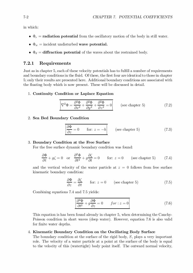
7-2 CHAPTER 7. POTENTIAL COEFFICIENTS
in which:
² ©r = radiation potential from the oscillatory motion of the body in still water.
² ©w = incident undisturbed wave potential.
² ©d = di¤raction potential of the waves about the restrained body.
7.2.1 Requirements
Just as in chapter 5, each of these velocity potentials has to ful…ll a number of requirementsand boundary conditions in the ‡uid. Of these, the …rst four are identical to those in chapter5; only their results are presented here. Additional boundary conditions are associated withthe ‡oating body which is now present. These will be discussed in detail.
1. Continuity Condition or Laplace Equation¯¯r2© =
@2©
@x2+@2©
@y2+@2©
@z2= 0
¯¯ (see chapter 5) (7.2)
2. Sea Bed Boundary Condition¯¯@©@z
= 0 for: z = ¡h¯¯ (see chapter 5) (7.3)
3. Boundary Condition at the Free SurfaceFor the free surface dynamic boundary condition was found:
@©
@t+ g³ = 0 or
@2©
@t2+ g
@³
@t= 0 for: z = 0 (see chapter 5) (7.4)
and the vertical velocity of the water particle at z = 0 follows from free surfacekinematic boundary condition:
@©
@z=@³
@tfor: z = 0 (see chapter 5) (7.5)
Combining equations 7.4 and 7.5 yields:
¯¯@2©@t2
+ g@©
@z= 0 for : z = 0
¯¯ (7.6)
This equation is has been found already in chapter 5, when determining the Cauchy-Poisson condition in short waves (deep water). However, equation 7.6 is also validfor …nite water depths.
4. Kinematic Boundary Condition on the Oscillating Body SurfaceThe boundary condition at the surface of the rigid body, S , plays a very importantrole. The velocity of a water particle at a point at the surface of the body is equalto the velocity of this (watertight) body point itself. The outward normal velocity,
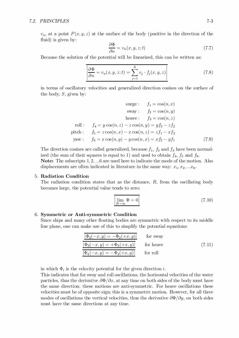
7.2. PRINCIPLES 7-3
vn, at a point P (x; y; z) at the surface of the body (positive in the direction of the‡uid) is given by:
@©
@n= vn(x; y; z; t) (7.7)
Because the solution of the potential will be linearized, this can be written as:
¯¯¯@©
@n= vn(x; y; z; t) =
6X
j=1
vj ¢ fj(x; y; z)¯¯¯ (7.8)
in terms of oscillatory velocities and generalized direction cosines on the surface ofthe body, S , given by:
surge : f1 = cos(n; x)
sway : f2 = cos(n; y)
heave : f3 = cos(n; z)
roll : f4 = y cos(n; z) ¡ z cos(n; y) = yf3 ¡ zf2pitch : f5 = z cos(n; x)¡ x cos(n; z) = zf1¡ xf3yaw : f6 = x cos(n; y) ¡ y cos(n; x) = xf2 ¡ yf1 (7.9)
The direction cosines are called generalized, because f1, f2 and f3 have been normal-ized (the sum of their squares is equal to 1) and used to obtain f4, f5 and f6.Note: The subscripts 1; 2; :::6 are used here to indicate the mode of the motion. Alsodisplacements are often indicated in literature in the same way: x1; x2; :::x6.
5. Radiation ConditionThe radiation condition states that as the distance, R, from the oscillating bodybecomes large, the potential value tends to zero:
¯¯ limR!1
© = 0¯¯ (7.10)
6. Symmetric or Anti-symmetric ConditionSince ships and many other ‡oating bodies are symmetric with respect to its middleline plane, one can make use of this to simplify the potential equations:
j©2(¡x; y) = ¡©2(+x; y)j for sway
j©3(¡x; y) = +©3(+x; y)j for heave (7.11)
j©4(¡x; y) = ¡©4(+x; y)j for roll
in which ©i is the velocity potential for the given direction i.This indicates that for sway and roll oscillations, the horizontal velocities of the waterparticles, thus the derivative @©=@x, at any time on both sides of the body must havethe same direction; these motions are anti-symmetric. For heave oscillations thesevelocities must be of opposite sign; this is a symmetric motion. However, for all threemodes of oscillations the vertical velocities, thus the derivative @©=@y, on both sidesmust have the same directions at any time.
7-4 CHAPTER 7. POTENTIAL COEFFICIENTS
7.2.2 Forces and Moments
The forces ~F and moments ~M follow from an integration of the pressure, p, over thesubmerged surface, S , of the body:
~F = ¡ZZ
S
(p ¢ ~n) ¢ dS
~M = ¡ZZ
S
p ¢ (~r £ ~n) ¢ dS (7.12)
in which ~n is the outward normal vector on surface dS and ~r is the position vector ofsurface dS in the O(x; y; z) coordinate system.The pressure p - via the linearized Bernoulli equation - is determined from the velocitypotentials by:
p = ¡½@©@t
¡ ½gz
= ¡½µ@©r@t
+@©w@t
+@©d@t
¶¡ ½gz (7.13)
which can obviously be split into four separate parts, so that the hydromechanical forces~F and moments ~M can be split into four parts too:
¯¯¯ ~F = ½
ZZ
S
µ@©r@t
+@©w@t
+@©d@t
+ gz
¶~n ¢ dS
¯¯¯ (7.14)
¯¯¯ ~M = ½
ZZ
S
µ@©r@t
+@©w@t
+@©d@t
+ gz
¶(~r £ ~n) ¢ dS
¯¯¯ (7.15)
or:
~F = ~Fr + ~Fw+ ~Fd + ~Fs~M = ~Mr + ~Mw+ ~Md + ~Ms (7.16)
Summarizing:
Source TermsWaves radiated from the oscillating body in still water ~Fr, ~Mr
Approaching waves on the …xed body ~Fw, ~Mw
Di¤racted waves of the …xed body ~Fd, ~Md
Hydrostatic buoyancy in still water ~Fs, ~Ms
These will each be discussed separately below.
7.2. PRINCIPLES 7-5
7.2.3 Hydrodynamic Loads
The hydrodynamic loads are the dynamic forces and moments caused by the ‡uid on anoscillating body in still water; waves are radiated from the body. The radiation potential,©r, which is associated with this oscillation in still water, can be written in terms, ©j, for6 degrees of freedom as:
©r(x; y; z; t) =6X
j=1
©j(x; y; z; t)
=6X
j=1
Áj(x; y; z) ¢ vj(t) (7.17)
in which the space and time dependent potential term, ©j(x; y; z; t) in direction j, is nowwritten in terms of a separate space dependent potential, Áj(x; y; z) in direction j, multi-plied by an oscillatory velocity, vj(t) in direction j.This allows the normal velocity on the surface of the body to be written as:
@©r@n
=@
@n
6X
j=1
©j
=6X
j=1
½@Áj@n
¢vj¾
(7.18)
and the generalized direction cosines, as given in equation 7.9, are given by:
fj =@Áj@n
(7.19)
With this, the radiation term in the hydrodynamic force of equation 7.14 becomes:
~Fr = ½
ZZ
S
µ@©r@t
¶~n ¢ dS
= ½
ZZ
S
Ã@
@t
6X
j=1
Ájvj
!~n ¢ dS (7.20)
and the moment term of equation 7.15 becomes:
~Mr = ½
ZZ
S
µ@©r@t
¶(~r £ ~n) ¢ dS
= ½
ZZ
S
Ã@
@t
6X
j=1
Ájvj
!(~r £ ~n) ¢ dS (7.21)
The components of these radiation forces and moments are de…ned by:
~Fr = (Xr1; Xr2 ; Xr3) and ~Mr = (Xr4; Xr5; Xr6) (7.22)

7-6 CHAPTER 7. POTENTIAL COEFFICIENTS
with (see 7.19):
~Xrk = ½
ZZ
S
Ã@
@t
6X
j=1
Ájvj
!fk ¢ dS
= ½
ZZ
S
Ã@
@t
6X
j=1
Ájvj
!@Ák@n
¢dS for: k = 1; :::6 (7.23)
Since Áj and Ák are not time-dependent in this expression, it reduces to:
¯¯¯Xrk =
6X
j=1
Xrkj
¯¯¯ for: k = 1; :::6 (7.24)
with: ¯¯¯Xrkj =
dvjdt½
Z Z
S
Áj@Ák@n
¢dS
¯¯¯ (7.25)
This radiation force or moment Xrkj in the direction k is caused by a forced harmonicoscillation of the body in the direction j . This is generally true for all j and k in the rangefrom 1 to 6. When j = k; the force or moment is caused by a motion in that same direction.When j 6= k; the force in one direction results from the motion in another direction. Thisintroduces what is called coupling between the forces and moments (or motions).The above equation expresses the force and moment components, Xrkj in terms of stillunknown potentials, Áj; not everything is solved yet! A solution for this will be found laterin this chapter.
Oscillatory Motion
Now an oscillatory motion is de…ned; suppose a motion (in a complex notation) given by:¯sj = saje¡i!t
¯(7.26)
Then the velocity and acceleration of this oscillation are:
_sj = vj = ¡i!saje¡i!t
Äsj =dvjdt= ¡!2saje¡i!t (7.27)
The hydrodynamic forces and moments can be split into a load in-phase with the acceler-ation and a load in-phase with the velocity:
Xrkj = ¡MkjÄsj ¡Nkj _sj=
¡saj!
2Mkj + isaj!Nkj¢e¡i!t
=
0@¡saj!2½
ZZ
S
Áj@Ák@n
¢dS
1A e¡i!t (7.28)
in which the last part is similar to the right hand side of equation 7.25.
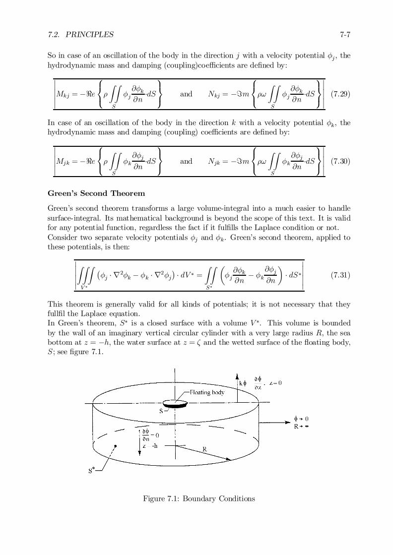
7.2. PRINCIPLES 7-7
So in case of an oscillation of the body in the direction j with a velocity potential Áj, thehydrodynamic mass and damping (coupling)coe¢cients are de…ned by:
¯¯¯Mkj = ¡<e
8<:½
ZZ
S
Áj@Ák@n
¢dS
9=; and Nkj = ¡=m
8<:½!
ZZ
S
Áj@Ák@n
¢dS
9=;
¯¯¯ (7.29)
In case of an oscillation of the body in the direction k with a velocity potential Ák, thehydrodynamic mass and damping (coupling) coe¢cients are de…ned by:
¯¯¯Mjk = ¡<e
8<:½
ZZ
S
Ák@Áj@n
¢dS
9=; and Njk = ¡=m
8<:½!
ZZ
S
Ák@Áj@n
¢dS
9=;
¯¯¯ (7.30)
Green’s Second Theorem
Green’s second theorem transforms a large volume-integral into a much easier to handlesurface-integral. Its mathematical background is beyond the scope of this text. It is validfor any potential function, regardless the fact if it ful…lls the Laplace condition or not.Consider two separate velocity potentials Áj and Ák. Green’s second theorem, applied tothese potentials, is then:
¯¯¯ZZZ
V ¤
¡Áj ¢ r2Ák ¡ Ák ¢ r2Áj
¢¢ dV ¤ =
ZZ
S¤
µÁj@Ák@n
¡ Ák@Áj@n
¶¢ dS¤
¯¯¯ (7.31)
This theorem is generally valid for all kinds of potentials; it is not necessary that theyfull…l the Laplace equation.In Green’s theorem, S¤ is a closed surface with a volume V ¤. This volume is boundedby the wall of an imaginary vertical circular cylinder with a very large radius R, the seabottom at z = ¡h, the water surface at z = ³ and the wetted surface of the ‡oating body,S ; see …gure 7.1.
Figure 7.1: Boundary Conditions
7-8 CHAPTER 7. POTENTIAL COEFFICIENTS
Both of the above radiation potentials Áj and Ák must ful…ll the Laplace equation 7.2:
r2Áj = r2Ák = 0 (7.32)
So the left hand side of equation 7.31 becomes zero, which yields for the right hand sideof equation 7.31: ZZ
S¤
Áj@Ák@n
¢dS¤ =ZZ
S¤
Ák@Áj@n
¢dS¤ (7.33)
The boundary condition at the free surface, equation 7.6, becomes for © = Á ¢ e¡i!t:
¡!2Á + g@Á@z= 0 for: z = 0 (7.34)
or with the dispersion relation, !2=g = k tanhkh:
k tanhkhÁ =@Á
@zfor: z = 0 (7.35)
This implies that at the free surface of the ‡uid one can write:
k tanhkh ¢ Ák = @Ák@z =
@Ák@n ¡!Ák = 1
k tanh kh ¢ @Ák@n
k tanhkh ¢Áj =@Áj@z=
@Áj@n
¡!Áj = 1k tanhkh
¢ @Áj@n
9=; at the free surface (7.36)
When taking also the boundary condition at the sea bed (equation 7.3) and the radiationcondition on the wall of the cylinder in …gure 7.1 (equation 7.10):
@Á
@n= 0 (for: z = ¡h) and lim
R!1Á = 0
into account, the integral equation 7.33 over the surface S¤ reduces to:
¯¯¯ZZ
S
Áj@Ák@n
¢dS =ZZ
S
Ák@Áj@n
¢dS
¯¯¯ (7.37)
in which S is the wetted surface of the body only.Note that in the light of the restriction introduced above, this is now (at least formally)only valid for deep water. The reader is also reminded that the Áj and Ák still have to beevaluated as well; this comes up again later in this chapter.
Potential Coe¢cients
A substitution of equation 7.37 in equations 7.29 and 7.30 provides symmetry - for thezero forward ship speed case - in the coe¢cients matrices with respect to their diagonalsso that:
Mjk = Mkj and Njk = Nkj (7.38)
7.2. PRINCIPLES 7-9
Because of the symmetry of a ship some coe¢cients are zero and the two matrices withhydrodynamic coe¢cients for ship become:
Hydrodynamic mass matrix:
0BBBBBB@
M11 0 M13 0 M15 00 M22 0 M24 0 M26
M31 0 M33 0 M35 00 M42 0 M44 0 M46
M51 0 M53 0 M55 00 M62 0 M64 0 M66
1CCCCCCA
(7.39)
Hydrodynamic damping matrix:
0BBBBBB@
N11 0 N13 0 N15 00 N22 0 N24 0 N26N31 0 N33 0 N35 00 N42 0 N44 0 N46N51 0 N53 0 N55 00 N62 0 N64 0 N66
1CCCCCCA
(7.40)
For clarity, the symmetry of terms about the diagonal in these matrices (for examplethat M13 = M31 for zero forward speed) has not been included here. The terms on thediagonals (such as Mnn for example) are the primary coe¢cients relating properties suchas hydrodynamic mass in one direction to the inertia forces in that same direction. O¤-diagonal terms (such as M13) represent hydrodynamic mass only which is associated withan inertia dependent force in one direction caused by a motion component in another.
Forward speed has an e¤ect on the velocity potentials, but is not discussed here. This e¤ectis quite completely explained by [Timman and Newman, 1962]. Another good reference is[Vugts, 1970].
7.2.4 Wave and Di¤raction Loads
The second and third term in 7.16 can be treated together. The wave and di¤raction termsin the hydrodynamic force and moment are:
~Fw+ ~Fd = ½
ZZ
S
µ@©w@t
+@©d@t
¶~n ¢ dS (7.41)
and:~Mw + ~Md = ½
ZZ
S
µ@©w@t
+@©d@t
¶(~r £ ~n) ¢ dS (7.42)
The principles of linear superposition allow the determination of these forces on a restrainedbody with zero forward speed; @©=@n = 0. This simpli…es the kinematic boundary condi-tion on the surface of the body to:
@©
@n=@©w@n
+@©d@n
= 0 (7.43)
The space and time dependent potentials, ©w(x; y; z; t) and ©d(x; y; z; t), are written nowin terms of isolated space dependent potentials, Áw(x; y; z) and Ád(x; y; z), multiplied by anormalized oscillatory velocity, v(t) = 1 ¢ e¡i!t:
©w(x; y; z; t) = Áw(x; y; z) ¢ e¡i!t©d(x; y; z; t) = Ád(x; y; z) ¢ e¡i!t (7.44)
7-10 CHAPTER 7. POTENTIAL COEFFICIENTS
Then from equation 7.43 follows:@Áw@n
= ¡@Ád@n
(7.45)
With this equation and equation 7.19 for the generalized direction cosines, one then …ndsthe wave forces and moments on the restrained body in waves:
Xwk = ¡i½e¡i!tZZ
S
(Áw+ Ád)fk ¢ dS
= ¡i½e¡i!tZZ
S
(Áw+ Ád)@Ák@n
¢dS for: k = 1; :::6 (7.46)
in which Ák is the radiation potential in direction k.The potential of the incident waves, Áw, is known (see chapter 5), but the di¤ractionpotential, Ád, has to be determined. Green’s second theorem from equation 7.37 providesa relation between this di¤raction potential, Ád, and a radiation potential, Ák:
ZZ
S
Ád@Ák@n
¢dS =ZZ
S
Ák@Ád@n
¢dS (7.47)
and with equation 7.45 one …nds:ZZ
S
Ád@Ák@n
¢dS = ¡ZZ
S
Ák@Áw@n
¢dS (7.48)
This elimination of the di¤raction potential results into the so-called Haskind relations:¯¯¯Xwk = ¡i½e¡i!t
ZZ
S
µÁw@Ák@n
+ Ák@Áw@n
¶¢ dS
¯¯¯ for: k = 1; :::6 (7.49)
This limits the problem of the di¤raction potential because the expression forXwk dependsonly on the wave potential Áw and the radiation potential Ák.
Note: These relations, found by [Haskind, 1957], are very important; they underlie therelative motion (displacement - velocity - acceleration) hypothesis, as used in chapter 6and in strip theory in chapter 8. These relations are valid only for a ‡oating body with azero time-averaged speed in all directions. [Newman, 1962] however, has generalized theHaskind relations for a body with a constant forward speed. He derived equations whichdi¤er only slightly from those found by Haskind. According to Newman’s approach thewave potential has to be de…ned in the moving O(x; y; z) system. The radiation potentialhas to be determined for the constant forward speed case, taking an opposite sign intoaccount.
The corresponding wave potential for deep water, as given in chapter 5, now becomes:
©w =³ag
!¢ekz ¢ sin(!t¡ kx cos¹¡ ky sin¹)
=i³ag
!¢ekz ¢ e¡ik(xcos¹+y sin ¹)e¡i!t (7.50)
7.2. PRINCIPLES 7-11
so that the isolated space dependent term is given by:
Áw =i³ag
!¢ ekz ¢ e¡ik(xcos¹+y sin¹) (7.51)
In these equations, ¹ is the wave direction.The velocity of the water particles in the direction of the outward normal n on the surfaceof the body is:
@Áw@n
=i³ag
!¢ k
½@z
@n¡ i
µ@x
@ncos¹+
@y
@nsin¹
¶¾¢ekz ¢ e¡ik(x cos ¹+y sin¹)
= Áw ¢ k ¢½@z
@n¡ i
µ@x
@ncos¹+
@y
@nsin¹
¶¾
= Áw ¢ k ¢ ff3 ¡ i (f1 cos¹+ f2 sin¹)g (7.52)
With this, the wave loads are given by:
Xwk = ¡i½!e¡i!tZZ
S
Áwfk ¢ dS
+i½!e¡i!tkZZ
S
ÁwÁk ff3¡ i (f1 cos¹+ f2 sin ¹)g ¢ dS
for: k = 1; :::6 (7.53)
The …rst term in this expression for the wave loads is the so-called Froude-Krilov force ormoment, which is the wave load caused by the undisturbed incident wave. The second termis caused by the wave disturbance due to the presence of the (…xed) body, the so-calleddi¤raction force.
7.2.5 Hydrostatic Loads
These buoyancy forces and moments are determined using the methods explained in chapter2. In the notation used here:
~Fs = ½g
ZZ
S
z~n ¢ dS and ~Ms = ½g
ZZ
S
z (~r x ~n) ¢ dS
or more generally:
¯¯¯Xsk = ½g
ZZ
S
zfk ¢ dS
¯¯¯ for: k = 1; :::6 (7.54)
in which the Xsk are the components of these hydrostatic forces and moments.
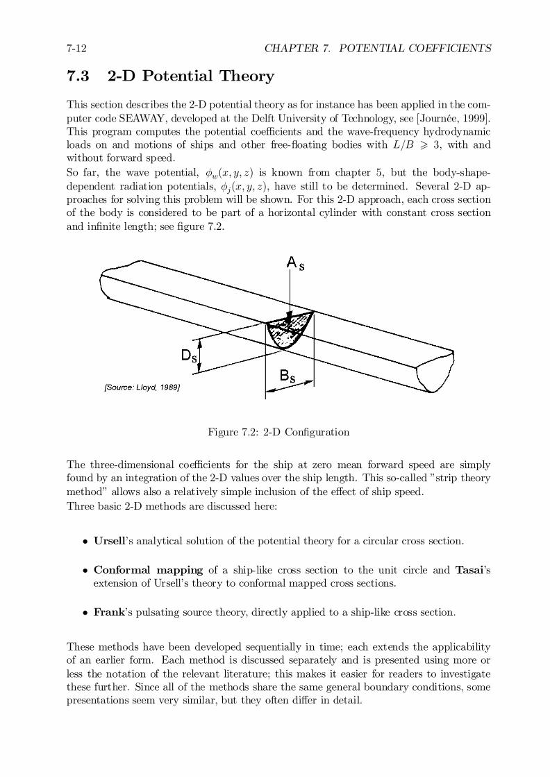
7-12 CHAPTER 7. POTENTIAL COEFFICIENTS
7.3 2-D Potential Theory
This section describes the 2-D potential theory as for instance has been applied in the com-puter code SEAWAY, developed at the Delft University of Technology, see [Journée, 1999].This program computes the potential coe¢cients and the wave-frequency hydrodynamicloads on and motions of ships and other free-‡oating bodies with L=B > 3, with andwithout forward speed.So far, the wave potential, Áw(x; y; z) is known from chapter 5, but the body-shape-dependent radiation potentials, Áj(x; y; z), have still to be determined. Several 2-D ap-proaches for solving this problem will be shown. For this 2-D approach, each cross sectionof the body is considered to be part of a horizontal cylinder with constant cross sectionand in…nite length; see …gure 7.2.
Figure 7.2: 2-D Con…guration
The three-dimensional coe¢cients for the ship at zero mean forward speed are simplyfound by an integration of the 2-D values over the ship length. This so-called ”strip theorymethod” allows also a relatively simple inclusion of the e¤ect of ship speed.Three basic 2-D methods are discussed here:
² Ursell’s analytical solution of the potential theory for a circular cross section.
² Conformal mapping of a ship-like cross section to the unit circle and Tasai’sextension of Ursell’s theory to conformal mapped cross sections.
² Frank’s pulsating source theory, directly applied to a ship-like cross section.
These methods have been developed sequentially in time; each extends the applicabilityof an earlier form. Each method is discussed separately and is presented using more orless the notation of the relevant literature; this makes it easier for readers to investigatethese further. Since all of the methods share the same general boundary conditions, somepresentations seem very similar, but they often di¤er in detail.
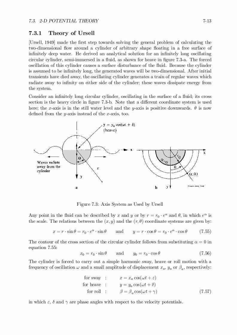
7.3. 2-D POTENTIAL THEORY 7-13
7.3.1 Theory of Ursell
[Ursell, 1949] made the …rst step towards solving the general problem of calculating thetwo-dimensional ‡ow around a cylinder of arbitrary shape ‡oating in a free surface ofin…nitely deep water. He derived an analytical solution for an in…nitely long oscillatingcircular cylinder, semi-immersed in a ‡uid, as shown for heave in …gure 7.3-a. The forcedoscillation of this cylinder causes a surface disturbance of the ‡uid. Because the cylinderis assumed to be in…nitely long, the generated waves will be two-dimensional. After initialtransients have died away, the oscillating cylinder generates a train of regular waves whichradiate away to in…nity on either side of the cylinder; these waves dissipate energy fromthe system.
Consider an in…nitely long circular cylinder, oscillating in the surface of a ‡uid; its crosssection is the heavy circle in …gure 7.3-b. Note that a di¤erent coordinate system is usedhere; the x-axis is in the still water level and the y-axis is positive downwards. µ is nowde…ned from the y-axis instead of the x-axis, too.
Figure 7.3: Axis System as Used by Ursell
Any point in the ‡uid can be described by x and y or by r = r0 ¢ e® and µ, in which e® isthe scale. The relations between the (x; y) and the (r; µ) coordinate systems are given by:
x = r ¢ sin µ = r0 ¢ e® ¢ sin µ and y = r ¢ cos µ = r0 ¢ e® ¢ cos µ (7.55)
The contour of the cross section of the circular cylinder follows from substituting ® = 0 inequation 7.55:
x0 = r0 ¢ sin µ and y0 = r0 ¢ cos µ (7.56)
The cylinder is forced to carry out a simple harmonic sway, heave or roll motion with afrequency of oscillation ! and a small amplitude of displacement xa, ya or ¯a, respectively:
for sway : x = xa cos(!t+ ")
for heave : y = ya cos(!t+ ±)
for roll : ¯ = ¯a cos(!t+ °) (7.57)
in which ", ± and ° are phase angles with respect to the velocity potentials.

7-14 CHAPTER 7. POTENTIAL COEFFICIENTS
The sway, heave and roll velocity and acceleration components of the cylinder are now:
for sway: _x = ¡!xa sin(!t+ ") and Äx = ¡!2xa cos(!t+ ")for heave: _y = ¡!ya sin(!t+ ±) and Äy = ¡!2ya cos(!t+ ±)for roll: _ = ¡!¯a sin(!t+ °) and Ä = ¡!2¯a cos(!t+ °) (7.58)
These forced oscillations of the cylinder cause a surface disturbance of the ‡uid. Becausethe cylinder is assumed to be in…nitely long, the generated waves will be two-dimensional.These waves travel away from the cylinder and a stationary state is rapidly attained; theydissipate the energy that the forced oscillation adds.
The ‡uid is assumed to be incompressible, inviscid and irrotational, without any e¤ects ofsurface tension. The motion amplitudes and velocities are small enough, so that all butthe linear terms of the free surface condition, the kinematic boundary condition on thecylinder and the Bernoulli equation may be neglected.
Boundary Conditions
For these oscillations, the two-dimensional velocity potentials of the ‡uid have to ful…ll thesix requirements as discussed in the …rst section of this chapter:
1. Laplace equation
r2© =@2©
@x2+@2©
@y2= 0 (7.59)
2. Sea bed boundary conditionThe boundary condition on the bottom in deep water is expressed by:
@©
@y!0 for: y ! 1 (7.60)
3. Free surface boundary conditionThe linearized free surface condition in deep water is expressed as follows:
@2©
@t2¡ g ¢ @©
@y= 0 or k©+
@©
@y= 0
for : jxj ¸ r0 and y = 0 with: k =!2
g(7.61)
In the polar coordinate system, this becomes:
¡»r ¢ e® ¢ ©§ @©
@µ= 0 for: ® ¸ 0 and µ = §¼
2(7.62)
in which »r is the non-dimensional frequency squared:
»r =!2
g¢r0 (7.63)
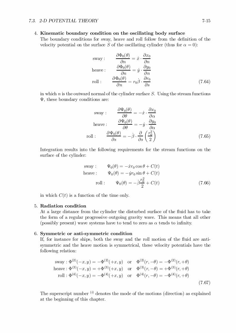
7.3. 2-D POTENTIAL THEORY 7-15
4. Kinematic boundary condition on the oscillating body surfaceThe boundary conditions for sway, heave and roll follow from the de…nition of thevelocity potential on the surface S of the oscillating cylinder (thus for ® = 0):
sway :@©0(µ)
@n= _x ¢ @x0
@n
heave :@©0(µ)
@n= _y ¢ @y0
@n
roll :@©0(µ)
@n= r0 _ ¢ @r0
@s(7.64)
in which n is the outward normal of the cylinder surface S. Using the stream functionsª, these boundary conditions are:
sway :@ª0(µ)
@µ= ¡ _x ¢ @x0
@®
heave :@ª0(µ)
@µ= ¡ _y ¢ @y0
@®
roll :@ª0(µ)
@s= ¡ _ ¢ @
@s
µr202
¶(7.65)
Integration results into the following requirements for the stream functions on thesurface of the cylinder:
sway : ª0(µ) = ¡ _xr0 cos µ + C(t)heave : ª0(µ) = ¡ _yr0 sin µ + C(t)
roll : ª0(µ) = ¡ _ r20
2+ C(t) (7.66)
in which C(t) is a function of the time only.
5. Radiation conditionAt a large distance from the cylinder the disturbed surface of the ‡uid has to takethe form of a regular progressive outgoing gravity wave. This means that all other(possibly present) wave systems have to tend to zero as ® tends to in…nity.
6. Symmetric or anti-symmetric conditionIf, for instance for ships, both the sway and the roll motion of the ‡uid are anti-symmetric and the heave motion is symmetrical, these velocity potentials have thefollowing relation:
sway : ©(2)(¡x; y) = ¡©(2)(+x; y) or ©(2)(r;¡µ) = ¡©(2)(r;+µ)heave : ©(3)(¡x; y) = +©(3)(+x; y) or ©(3)(r;¡µ) = +©(3)(r;+µ)
roll : ©(4)(¡x; y) = ¡©(4)(+x; y) or ©(4)(r;¡µ) = ¡©(4)(r;+µ)(7.67)
The superscript number (i) denotes the mode of the motions (direction) as explainedat the beginning of this chapter.
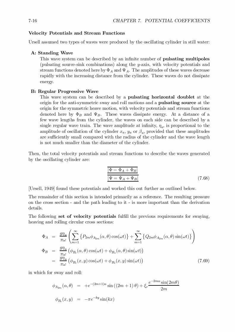
7-16 CHAPTER 7. POTENTIAL COEFFICIENTS
Velocity Potentials and Stream Functions
Ursell assumed two types of waves were produced by the oscillating cylinder in still water:
A: Standing WaveThis wave system can be described by an in…nite number of pulsating multipoles(pulsating source-sink combinations) along the y-axis, with velocity potentials andstream functions denoted here by©A andªA. The amplitudes of these waves decreaserapidly with the increasing distance from the cylinder. These waves do not dissipateenergy.
B: Regular Progressive WaveThis wave system can be described by a pulsating horizontal doublet at theorigin for the anti-symmetric sway and roll motions and a pulsating source at theorigin for the symmetric heave motion, with velocity potentials and stream functionsdenoted here by ©B and ªB. These waves dissipate energy. At a distance of afew wave lengths from the cylinder, the waves on each side can be described by asingle regular wave train. The wave amplitude at in…nity, ´a, is proportional to theamplitude of oscillation of the cylinder xa, ya or ¯a, provided that these amplitudesare su¢ciently small compared with the radius of the cylinder and the wave lengthis not much smaller than the diameter of the cylinder.
Then, the total velocity potentials and stream functions to describe the waves generatedby the oscillating cylinder are:
j© = ©A + ©Bjjª = ªA +ªBj (7.68)
[Ursell, 1949] found these potentials and worked this out further as outlined below.
The remainder of this section is intended primarily as a reference. The resulting pressureon the cross section - and the path leading to it - is more important than the derivationdetails.
The following set of velocity potentials ful…ll the previous requirements for swaying,heaving and rolling circular cross sections:
©A =g´a¼!
à 1X
m=1
©P2mÁA2m(®; µ) cos(!t)
ª+
1X
m=1
©Q2mÁA2m(®; µ) sin(!t)
ª!
©B =g´a¼!
¡ÁBc(®; µ) cos(!t) + ÁBs(®; µ) sin(!t)
¢
=g´a¼!
¡ÁBc(x; y) cos(!t) + ÁBs(x; y) sin(!t)
¢(7.69)
in which for sway and roll:
ÁA2m (®; µ) = +e¡(2m+1)® sin ((2m +1) µ) + »re¡2m® sin(2mµ)
2m
ÁBc(x; y) = ¡¼e¡ky sin(kx)
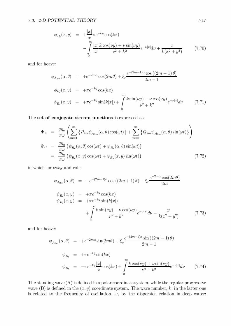
7.3. 2-D POTENTIAL THEORY 7-17
ÁBs(x; y) = +jxjx¼e¡ky cos(kx)
¡1Z
0
jxjx
k cos(ºy) + º sin(ºy)
º2 + k2e¡ºjxjdº +
x
k(x2 + y2)(7.70)
and for heave:
ÁA2m(®; µ) = +e¡2m® cos(2mµ) + »re¡(2m¡1)® cos ((2m¡ 1) µ)
2m¡ 1
ÁBc(x; y) = +¼e¡ky cos(kx)
ÁBs(x; y) = +¼e¡ky sin(kjxj) +1Z
0
k sin(ºy)¡ º cos(ºy)º2 + k2
e¡ºjxjdº (7.71)
The set of conjugate stream functions is expressed as:
ªA =g´a¼!
à 1X
m=1
©P2mÃA2m(®; µ)cos(!t)
ª+
1X
m=1
©Q2mÃA2m(®; µ) sin(!t)
ª!
ªB =g´a¼!
¡ÃBc(®; µ)cos(!t) +ÃBs(®; µ) sin(!t)
¢
=g´a¼!
¡ÃBc(x; y) cos(!t) + ÃBs(x; y) sin(!t)
¢(7.72)
in which for sway and roll:
ÃA2m(®; µ) = ¡e¡(2m+1)® cos ((2m+ 1) µ)¡ »re¡2m® cos(2mµ)
2m
ÃBc(x; y) = +¼e¡ky cos(kx)
ÃBs(x; y) = +¼e¡ky sin(kjxj)
+
1Z
0
k sin(ºy)¡ º cos(ºy)º2+ k2
e¡ºjxjdº ¡ y
k(x2 + y2)(7.73)
and for heave:
ÃA2m(®; µ) = +e¡2m® sin(2mµ) + »re¡(2m¡1)® sin ((2m ¡ 1) µ)
2m¡ 1
ÃBc = +¼e¡ky sin(kx)
ÃBs = ¡¼e¡ky jxjxcos(kx) +
1Z
0
k cos(ºy) + º sin(ºy)
º2 + k2e¡ºjxjdº (7.74)
The standing wave (A) is de…ned in a polar coordinate system, while the regular progressivewave (B) is de…ned in the (x; y) coordinate system. The wave number, k, in the latter oneis related to the frequency of oscillation, !, by the dispersion relation in deep water:
7-18 CHAPTER 7. POTENTIAL COEFFICIENTS
k = !2=g. The variable º has the dimension of the wave number k; it is not the kinematicviscosity here.Notice the symmetric and anti-symmetric relations in the set of velocity potentials andstream functions.The unknowns P2m and Q2m in these equations have to be found; they follow from theboundary conditions in the ‡uid.
Solution
The stream functions for sway, heave and roll on the surface of the cylinder (® = 0)reduce to:
ª0(µ) =g´a¼!
(ÃÃB0c(µ) +
1X
m=1
©P2mÃA02m(µ)
ª!cos(!t)
+
ÃÃB0s(µ) +
1X
m=1
©Q2mÃA02m(µ)
ª!sin(!t)
)(7.75)
in which:
for sway and roll : ÃA02m(µ) = cos ((2m+ 1)µ) + »rcos(2mµ)
2m
for heave : ÃA02m(µ) = sin(2mµ) + »rsin ((2m ¡ 1)µ)
2m¡ 1 (7.76)
where ÃB0c(µ) and ÃB0s(µ) are the values of ÃBc(®; µ) and ÃBs(®; µ) at the surface of thecylinder and »r is the non-dimensional frequency of oscillation squared.These expressions for the stream functions should be equal to the stream functions thatsatisfy the kinematic boundary conditions on the surface of the oscillating cylinder, givenin equations 7.66. Doing this makes it possible to determine the values for the P2m andQ2m series of values as well as the amplitude ratios xa=´a, ya=´a and ¯a=k´a and the phaseshifts ", ± and °.
Once the P2m and Q2m series of values have been found, the velocity potentials forsway, heave and roll can be determined, too:
©0(µ) =g´a¼!
(ÃÁB0c(µ) +
1X
m=1
©P2mÁA02m(µ)
ª!cos(!t)
+
ÃÁB0s(µ) +
1X
m=1
©Q2mÁA02m(µ)
ª!sin(!t)
)(7.77)
in which:
for sway and roll : ÁA02m(µ) = sin ((2m +1)µ) + »rsin(2mµ)
2m
for heave : ÁA02m(µ) = cos(2mµ) + »rcos ((2m¡ 1)µ)
2m¡ 1 (7.78)
7.3. 2-D POTENTIAL THEORY 7-19
Hydrodynamic Pressure
With known velocity potentials, the hydrodynamic pressure on the surface of the cylindercan be obtained from the linearized Bernoulli equation 7.13:
p(µ) = ¡½@©0(µ)@t
=¡½g´a¼
(ÃÁB0s(µ) +
1X
m=1
©Q2mÁA02m(µ)
ª!cos(!t)
¡ÃÁB0c(µ) +
1X
m=1
©P2mÁA02m(µ)
ª!sin(!t)
)(7.79)
where ÁB0c(µ) and ÁB0s(µ) are the values of ÁBc(®; µ) and ÁBs(®; µ) at the surface of thecylinder.It is obvious that the pressures for sway and roll are skew-symmetric in µ, thus p(¡µ) =¡p(+µ), and symmetric in µ for heave, thus: p(¡µ) = p(+µ).
Hydrodynamic Loads
The two-dimensional hydrodynamic sway and heave force and roll moment can be obtainedfrom integrations of these pressures over the contour, C0 at r = r0, of the circular crosssection. When switching to polar coordinates, derivatives with respect to µ have to beused:
dx0dµ
= +r0 cos µ anddy0dµ
= ¡r0 sin µ (7.80)
With these, the loads can be expressed in terms of potential mass and damping, as equations7.81, 7.82 and 7.83 show. A comparison of the in-phase terms (cos(!t)) in each of theseequations provides the potential mass coe¢cients, while a comparison of the out-of-phaseterms (sin(!t)) the potential damping coe¢cients provides.
Fx0 =
Z
C0
p(µ)dy0 = 2
12 ¼Z
0
p(µ)dy0dµdµ
8><>:= ¡2r0
12 ¼Z
0
p(µ) sin µ dµ (for this circular cylinder)
9>=>;
= ¡M220 ¢ Äx ¡N22 0 ¢ _x (for a swaying cylinder)
= ¡M240 ¢ Ä ¡N24 0 ¢ _ (for a rolling cylinder) (7.81)
Fy0 = ¡
Z
C0
p(µ)dx0 = ¡2
12¼Z
0
p(µ)dx0dµdµ
8><>:= ¡2r0
12 ¼Z
0
p(µ) cos µ dµ (for this circular cylinder)
9>=>;
7-20 CHAPTER 7. POTENTIAL COEFFICIENTS
= ¡M330 ¢ Äy ¡N330 ¢ _y (for a heaving cylinder) (7.82)
MR0 = ¡
Z
C0
p(µ)x0dx0 ¡Z
C0
p(µ)y0dy0
= ¡2
12¼Z
0
p(µ)
µx0dx0dµ
+ y0dy0dµ
¶dµ
8><>:= ¡2r02
12¼Z
0
p(µ)(sin µ cos µ¡ sin µ cos µ) dµ = 0 (for this circular cylinder)
9>=>;
= ¡M420 ¢ Äx ¡N42 0 ¢ _x (for a swaying cylinder)
= ¡M440 ¢ Ä ¡N44 0 ¢ _ (for a rolling cylinder) (7.83)
with:
M220 = 2-D hydrodynamic mass coe¢cient of sway
N220 = 2-D hydrodynamic damping coe¢cient of sway
M420 = 2-D hydrodynamic mass coupling coe¢cient of sway into roll
N420 = 2-D hydrodynamic damping coupling coe¢cient of sway into roll
M330 = 2-D hydrodynamic mass coe¢cient of heave
N330 = 2-D hydrodynamic damping coe¢cient of heave
M240 = 2-D hydrodynamic mass coupling coe¢cient of roll into sway
N240 = 2-D hydrodynamic damping coupling coe¢cient of roll into sway
M440 = 2-D hydrodynamic mass moment of inertia coe¢cient of roll
N440 = 2-D hydrodynamic damping coe¢cient of roll
7.3.2 Conformal Mapping
Ursell’s derivation is valid only for a circular cross section. Since few ships have this shape,a method is needed to transform realistic shapes so that ”it looks like” a circular cylinderin Ursell’s method.
More or less arbitrary, but still symmetrical, cross sections can be mapped conformal to aunit circle. The general transformation formula to do this is given by:
¯¯¯z = Ms
NX
n=0
na2n¡1³
¡(2n¡1)o¯¯¯ (7.84)
with:
z = x + iy = speci…es the ship’s cross section shape (…gure 7.4-b)³ = ie®e¡iµ = speci…es the circular cross section shape (…gure 7.4-a)Ms = scale factora¡1 = +1a2n¡1 = conformal mapping coe¢cients (n = 1; :::; N )N = number of parameters used
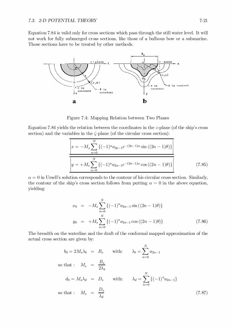
7.3. 2-D POTENTIAL THEORY 7-21
Equation 7.84 is valid only for cross sections which pass through the still water level. It willnot work for fully submerged cross sections, like those of a bulbous bow or a submarine.Those sections have to be treated by other methods.
Figure 7.4: Mapping Relation between Two Planes
Equation 7.84 yields the relation between the coordinates in the z-plane (of the ship’s crosssection) and the variables in the ³-plane (of the circular cross section):
¯¯¯x = ¡Ms
NX
n=0
f(¡1)na2n¡1e¡(2n¡1)® sin ((2n¡ 1)µ)g¯¯¯
¯¯¯y = +Ms
NX
n=0
f(¡1)na2n¡1e¡(2n¡1)® cos ((2n¡ 1)µ)g¯¯¯ (7.85)
® = 0 in Ursell’s solution corresponds to the contour of his circular cross section. Similarly,the contour of the ship’s cross section follows from putting ® = 0 in the above equation,yielding:
x0 = ¡Ms
NX
n=0
f(¡1)na2n¡1 sin ((2n¡ 1)µ)g
y0 = +Ms
NX
n=0
f(¡1)na2n¡1 cos ((2n¡ 1)µ)g (7.86)
The breadth on the waterline and the draft of the conformal mapped approximation of theactual cross section are given by:
b0 = 2Ms¸b = Bs with: ¸b =NX
n=0
a2n¡1
so that : Ms =Bs2¸b
d0 = Ms¸d = Ds with: ¸d =NX
n=0
f(¡1)na2n¡1g
so that : Ms =Ds¸d
(7.87)
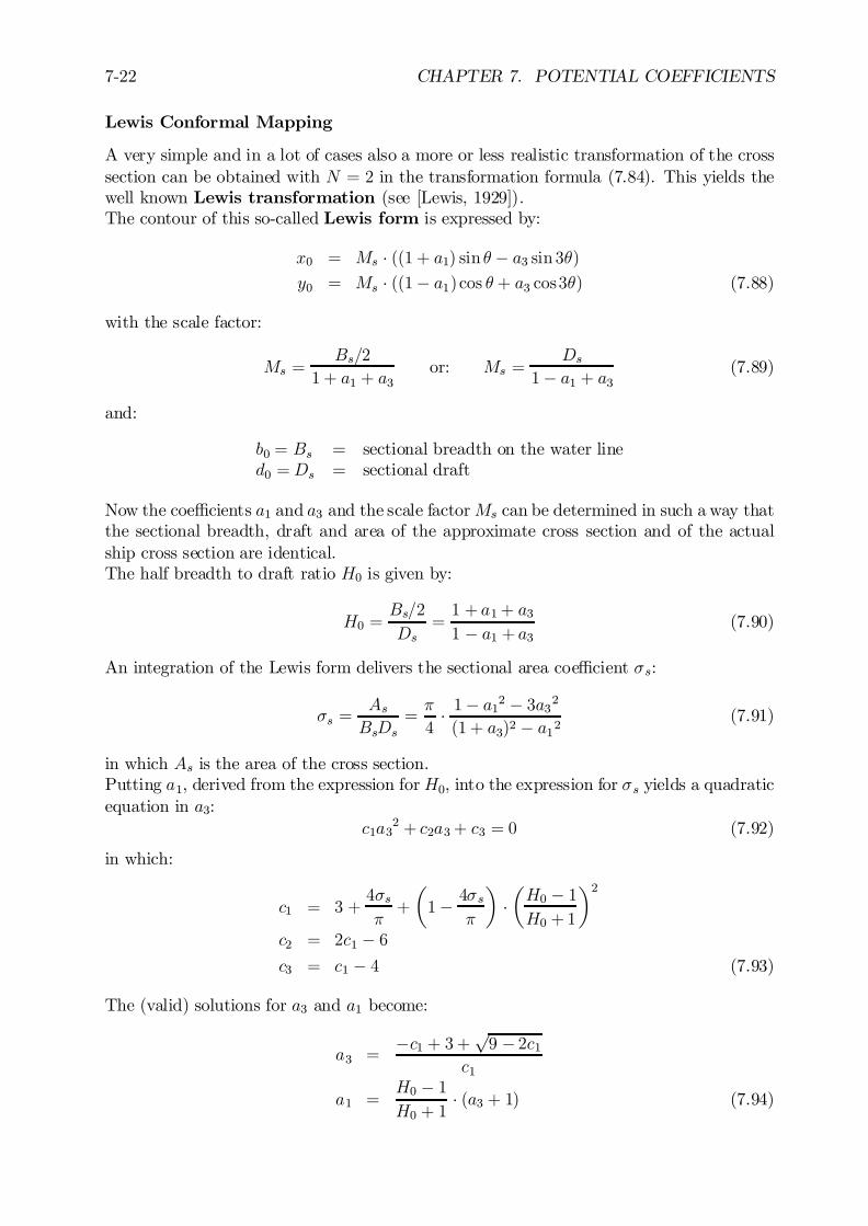
7-22 CHAPTER 7. POTENTIAL COEFFICIENTS
Lewis Conformal Mapping
A very simple and in a lot of cases also a more or less realistic transformation of the crosssection can be obtained with N = 2 in the transformation formula (7.84). This yields thewell known Lewis transformation (see [Lewis, 1929]).The contour of this so-called Lewis form is expressed by:
x0 = Ms ¢ ((1 + a1) sin µ¡ a3 sin 3µ)y0 = Ms ¢ ((1¡ a1)cos µ + a3 cos3µ) (7.88)
with the scale factor:
Ms =Bs=2
1 + a1 + a3or: Ms =
Ds1¡ a1 + a3
(7.89)
and:
b0 = Bs = sectional breadth on the water lined0 =Ds = sectional draft
Now the coe¢cients a1 and a3 and the scale factorMs can be determined in such a way thatthe sectional breadth, draft and area of the approximate cross section and of the actualship cross section are identical.The half breadth to draft ratio H0 is given by:
H0 =Bs=2
Ds=1 + a1+ a31 ¡ a1 + a3
(7.90)
An integration of the Lewis form delivers the sectional area coe¢cient ¾s:
¾s =AsBsDs
=¼
4¢ 1¡ a12 ¡ 3a32(1 + a3)2 ¡ a12
(7.91)
in which As is the area of the cross section.Putting a1, derived from the expression forH0, into the expression for ¾s yields a quadraticequation in a3:
c1a32 + c2a3+ c3 = 0 (7.92)
in which:
c1 = 3 +4¾s¼+
µ1¡ 4¾s
¼
¶¢µH0 ¡ 1H0 +1
¶2
c2 = 2c1 ¡ 6c3 = c1 ¡ 4 (7.93)
The (valid) solutions for a3 and a1 become:
a3 =¡c1 + 3+
p9 ¡ 2c1
c1
a1 =H0 ¡ 1H0 + 1
¢ (a3 + 1) (7.94)
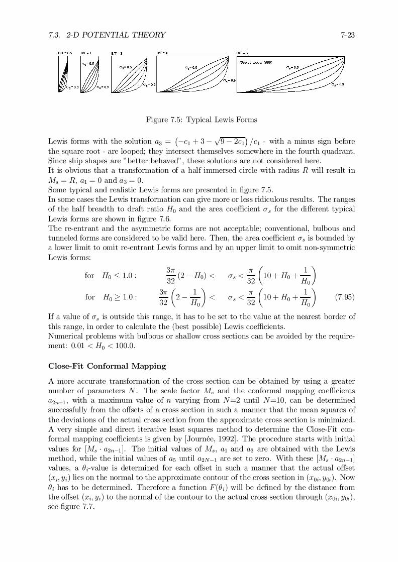
7.3. 2-D POTENTIAL THEORY 7-23
Figure 7.5: Typical Lewis Forms
Lewis forms with the solution a3 =¡¡c1 + 3¡ p
9¡ 2c1¢=c1 - with a minus sign before
the square root - are looped; they intersect themselves somewhere in the fourth quadrant.Since ship shapes are ”better behaved”, these solutions are not considered here.It is obvious that a transformation of a half immersed circle with radius R will result inMs = R, a1 = 0 and a3 = 0.Some typical and realistic Lewis forms are presented in …gure 7.5.In some cases the Lewis transformation can give more or less ridiculous results. The rangesof the half breadth to draft ratio H0 and the area coe¢cient ¾s for the di¤erent typicalLewis forms are shown in …gure 7.6.The re-entrant and the asymmetric forms are not acceptable; conventional, bulbous andtunneled forms are considered to be valid here. Then, the area coe¢cient ¾s is bounded bya lower limit to omit re-entrant Lewis forms and by an upper limit to omit non-symmetricLewis forms:
for H0 · 1:0 :3¼
32(2¡H0) < ¾s <
¼
32
µ10 +H0 +
1
H0
¶
for H0 ¸ 1:0 :3¼
32
µ2¡ 1
H0
¶< ¾s <
¼
32
µ10 +H0 +
1
H0
¶(7.95)
If a value of ¾s is outside this range, it has to be set to the value at the nearest border ofthis range, in order to calculate the (best possible) Lewis coe¢cients.Numerical problems with bulbous or shallow cross sections can be avoided by the require-ment: 0:01 < H0 < 100:0.
Close-Fit Conformal Mapping
A more accurate transformation of the cross section can be obtained by using a greaternumber of parameters N . The scale factor Ms and the conformal mapping coe¢cientsa2n¡1, with a maximum value of n varying from N=2 until N=10, can be determinedsuccessfully from the o¤sets of a cross section in such a manner that the mean squares ofthe deviations of the actual cross section from the approximate cross section is minimized.A very simple and direct iterative least squares method to determine the Close-Fit con-formal mapping coe¢cients is given by [Journée, 1992]. The procedure starts with initialvalues for [Ms ¢ a2n¡1]. The initial values of Ms, a1 and a3 are obtained with the Lewismethod, while the initial values of a5 until a2N¡1 are set to zero. With these [Ms ¢ a2n¡1]values, a µi-value is determined for each o¤set in such a manner that the actual o¤set(xi; yi) lies on the normal to the approximate contour of the cross section in (x0i; y0i). Nowµi has to be determined. Therefore a function F (µi) will be de…ned by the distance fromthe o¤set (xi; yi) to the normal of the contour to the actual cross section through (x0i; y0i),see …gure 7.7.
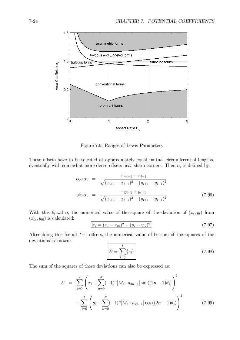
7-24 CHAPTER 7. POTENTIAL COEFFICIENTS
Figure 7.6: Ranges of Lewis Parameters
These o¤sets have to be selected at approximately equal mutual circumferential lengths,eventually with somewhat more dense o¤sets near sharp corners. Then ®i is de…ned by:
cos®i =+xi+1¡ xi¡1p
(xi+1 ¡ xi¡1)2 + (yi+1 ¡ yi¡1)2
sin®i =¡yi+1 + yi¡1p
(xi+1 ¡ xi¡1)2 + (yi+1 ¡ yi¡1)2(7.96)
With this µi-value, the numerical value of the square of the deviation of (xi; yi) from(x0i; y0i) is calculated:
jei = (xi ¡ x0i)2 + (yi ¡ y0i)2j (7.97)
After doing this for all I+1 o¤sets, the numerical value of he sum of the squares of thedeviations is known: ¯
¯¯E =
IX
i=0
feig¯¯¯ (7.98)
The sum of the squares of these deviations can also be expressed as:
E =IX
i=0
Ãxi +
NX
n=0
(¡1)n[Ms ¢ a2n¡1] sin ((2n¡ 1)µi)!2
+IX
i=0
Ãyi ¡
NX
n=0
(¡1)n[Ms ¢ a2n¡1] cos ((2n¡ 1)µi)!2
(7.99)

7.3. 2-D POTENTIAL THEORY 7-25
Figure 7.7: Close-Fit Conformal Mapping De…nitions
Then new values of [Ms ¢ a2n¡1] have to be obtained in such a manner that E is minimized.This means that each of the derivatives of this equation with respect to each coe¢cient[Ms ¢ a2n¡1] is zero, so:
¯¯ @E
@fMsa2j¡1g= 0
¯¯ for: j = 0; :::N (7.100)
This yields N+1 equations:NX
n=0
((¡1)n[Ms ¢ a2n¡1]
IX
i=0
cos((2j ¡ 2n)µi))
=IX
i=0
f¡xi sin ((2j ¡ 1)µi) + yi cos ((2j ¡ 1)µi)g
for: j = 0; :::N (7.101)
To obtain the exact breadth and draft, the last two equations are replaced by the equationsfor the breadth at the waterline and the draft:
NX
n=0
((¡1)n[Ms ¢ a2n¡1]
IX
i=0
cos((2j ¡ 2n)µi))
=IX
i=0
f¡xi sin ((2j ¡ 1)µi) + yi cos ((2j ¡ 1)µi)g
for: j = 0; :::N ¡ 2NX
n=0
f [Ms ¢ a2n¡1]g = Bs=2 j = N ¡ 1
NX
n=0
f (¡1)n[Ms ¢ a2n¡1]g = Ds j = N (7.102)
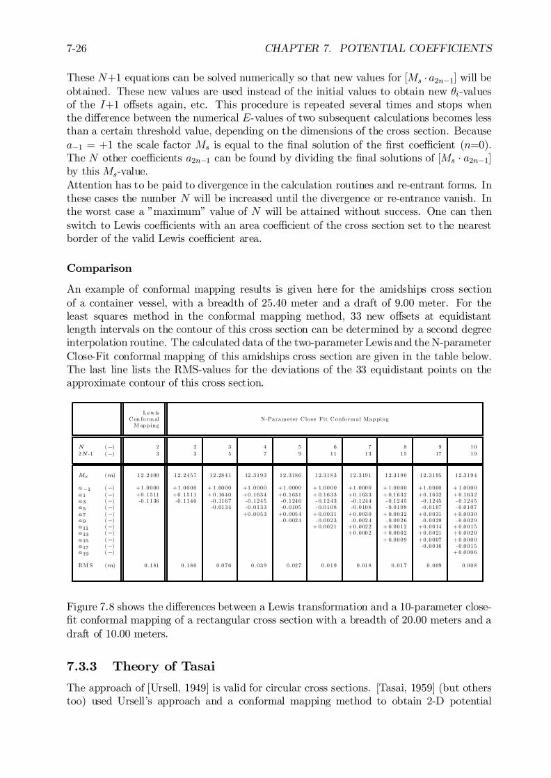
7-26 CHAPTER 7. POTENTIAL COEFFICIENTS
These N+1 equations can be solved numerically so that new values for [Ms ¢ a2n¡1] will beobtained. These new values are used instead of the initial values to obtain new µi-valuesof the I+1 o¤sets again, etc. This procedure is repeated several times and stops whenthe di¤erence between the numerical E-values of two subsequent calculations becomes lessthan a certain threshold value, depending on the dimensions of the cross section. Becausea¡1 = +1 the scale factor Ms is equal to the …nal solution of the …rst coe¢cient (n=0).The N other coe¢cients a2n¡1 can be found by dividing the …nal solutions of [Ms ¢ a2n¡1]by this Ms-value.Attention has to be paid to divergence in the calculation routines and re-entrant forms. Inthese cases the number N will be increased until the divergence or re-entrance vanish. Inthe worst case a ”maximum” value of N will be attained without success. One can thenswitch to Lewis coe¢cients with an area coe¢cient of the cross section set to the nearestborder of the valid Lewis coe¢cient area.
Comparison
An example of conformal mapping results is given here for the amidships cross sectionof a container vessel, with a breadth of 25.40 meter and a draft of 9.00 meter. For theleast squares method in the conformal mapping method, 33 new o¤sets at equidistantlength intervals on the contour of this cross section can be determined by a second degreeinterpolation routine. The calculated data of the two-parameter Lewis and the N-parameterClose-Fit conformal mapping of this amidships cross section are given in the table below.The last line lists the RMS-values for the deviations of the 33 equidistant points on theapproximate contour of this cross section.
Le w isCon form al N-Param eter C lose Fit Conform al Map ping
M ap ping
N (¡) 2 2 3 4 5 6 7 8 9 102N -1 (¡) 3 3 5 7 9 11 13 15 17 19
Ms (m) 12 .2400 12 .2457 12 .2841 12 .3193 12 .3186 12.3183 12 .3191 12.3190 12 .3195 12 .3194
a¡1 (¡) +1 .0000 +1.0000 + 1.0000 +1.0000 +1.0000 + 1.0000 +1.0000 + 1.0000 +1.0000 + 1.0000a1 (¡) +0 .1511 +0.1511 + 0.1640 +0.1634 +0.1631 + 0.1633 +0.1633 + 0.1632 +0.1632 + 0.1632a3 (¡) -0 .1136 -0 .1140 -0 .1167 -0 .1245 -0 .1246 - 0.1243 -0 .1244 - 0.1245 -0 .1245 - 0 .1245a5 (¡) -0 .0134 -0 .0133 -0 .0105 - 0.0108 -0 .0108 - 0.0108 -0 .0107 - 0 .0107a7 (¡) +0 .0053 +0.0054 + 0.0031 +0.0030 + 0.0032 +0.0031 + 0.0030a9 (¡) -0 .0024 - 0.0023 -0 .0024 - 0.0026 -0 .0029 - 0 .0029a11 (¡) + 0.0021 +0.0022 + 0.0012 +0.0014 + 0.0015a13 (¡) +0 .0002 + 0.0002 +0.0021 + 0.0020a15 (¡) + 0.0009 +0.0007 + 0.0000a17 (¡) -0 .0016 - 0 .0015a19 (¡) + 0 .0006
RM S (m) 0 .181 0 .180 0 .076 0 .039 0 .027 0 .019 0 .018 0 .017 0 .009 0.008
Figure 7.8 shows the di¤erences between a Lewis transformation and a 10-parameter close-…t conformal mapping of a rectangular cross section with a breadth of 20.00 meters and adraft of 10.00 meters.
7.3.3 Theory of Tasai
The approach of [Ursell, 1949] is valid for circular cross sections. [Tasai, 1959] (but otherstoo) used Ursell’s approach and a conformal mapping method to obtain 2-D potential
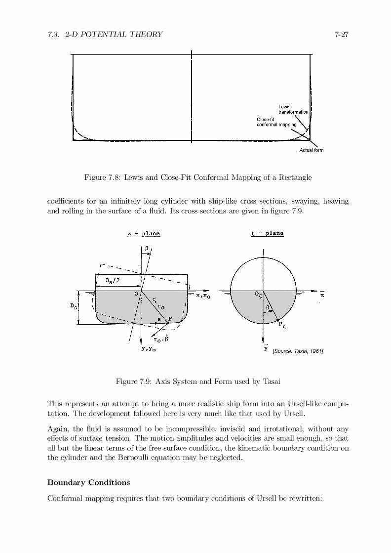
7.3. 2-D POTENTIAL THEORY 7-27
Figure 7.8: Lewis and Close-Fit Conformal Mapping of a Rectangle
coe¢cients for an in…nitely long cylinder with ship-like cross sections, swaying, heavingand rolling in the surface of a ‡uid. Its cross sections are given in …gure 7.9.
Figure 7.9: Axis System and Form used by Tasai
This represents an attempt to bring a more realistic ship form into an Ursell-like compu-tation. The development followed here is very much like that used by Ursell.
Again, the ‡uid is assumed to be incompressible, inviscid and irrotational, without anye¤ects of surface tension. The motion amplitudes and velocities are small enough, so thatall but the linear terms of the free surface condition, the kinematic boundary condition onthe cylinder and the Bernoulli equation may be neglected.
Boundary Conditions
Conformal mapping requires that two boundary conditions of Ursell be rewritten:
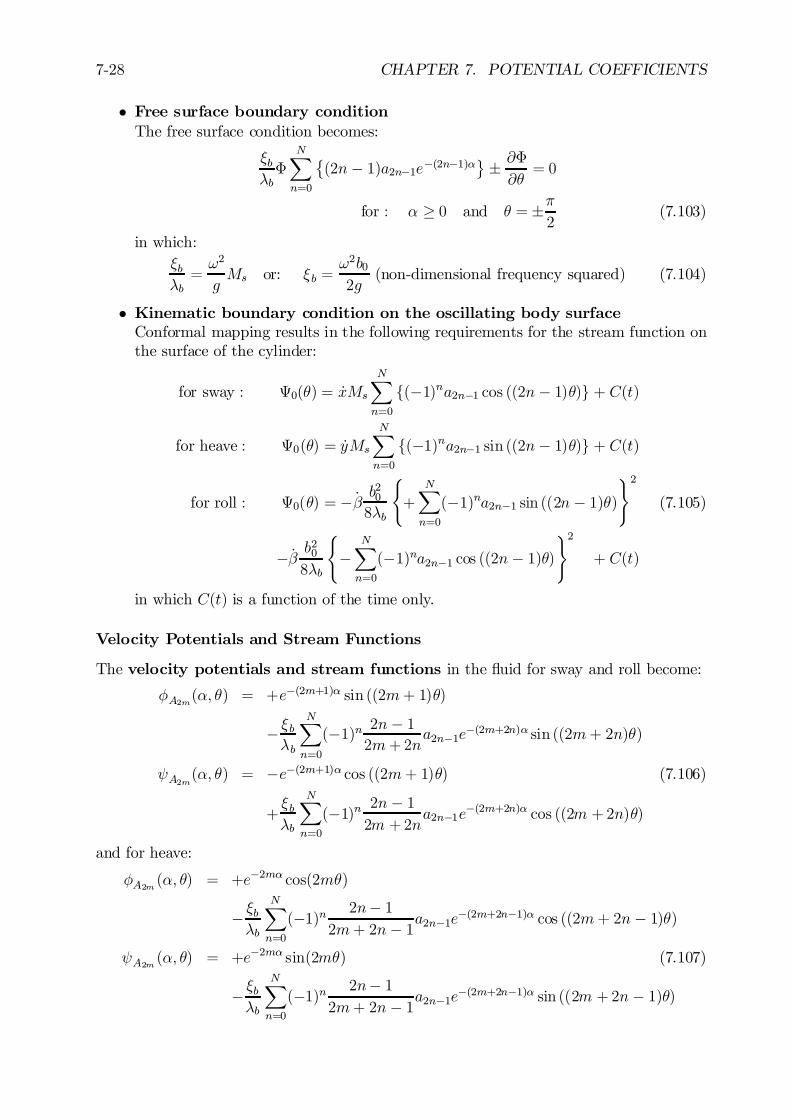
7-28 CHAPTER 7. POTENTIAL COEFFICIENTS
² Free surface boundary conditionThe free surface condition becomes:
»b¸b©
NX
n=0
©(2n¡ 1)a2n¡1e¡(2n¡1)®
ª§ @©
@µ= 0
for : ® ¸ 0 and µ = §¼2
(7.103)
in which:»b¸b=!2
gMs or: »b =
!2b02g
(non-dimensional frequency squared) (7.104)
² Kinematic boundary condition on the oscillating body surfaceConformal mapping results in the following requirements for the stream function onthe surface of the cylinder:
for sway : ª0(µ) = _xMs
NX
n=0
f(¡1)na2n¡1 cos ((2n¡ 1)µ)g + C(t)
for heave : ª0(µ) = _yMs
NX
n=0
f(¡1)na2n¡1 sin ((2n¡ 1)µ)g + C(t)
for roll : ª0(µ) = ¡ _ b20
8¸b
(+
NX
n=0
(¡1)na2n¡1 sin ((2n¡ 1)µ))2
(7.105)
¡ _ b20
8¸b
(¡
NX
n=0
(¡1)na2n¡1 cos ((2n¡ 1)µ))2
+ C(t)
in which C(t) is a function of the time only.
Velocity Potentials and Stream Functions
The velocity potentials and stream functions in the ‡uid for sway and roll become:
ÁA2m(®; µ) = +e¡(2m+1)® sin ((2m+ 1)µ)
¡ »b¸b
NX
n=0
(¡1)n 2n¡ 12m+2n
a2n¡1e¡(2m+2n)® sin ((2m+ 2n)µ)
ÃA2m(®; µ) = ¡e¡(2m+1)® cos ((2m+ 1)µ) (7.106)
+»b¸b
NX
n=0
(¡1)n 2n¡ 12m +2n
a2n¡1e¡(2m+2n)® cos ((2m +2n)µ)
and for heave:
ÁA2m (®; µ) = +e¡2m® cos(2mµ)
¡ »b¸b
NX
n=0
(¡1)n 2n¡ 12m+ 2n¡ 1a2n¡1e
¡(2m+2n¡1)® cos ((2m+ 2n¡ 1)µ)
ÃA2m (®; µ) = +e¡2m® sin(2mµ) (7.107)
¡ »b¸b
NX
n=0
(¡1)n 2n¡ 12m+ 2n¡ 1a2n¡1e
¡(2m+2n¡1)® sin ((2m +2n¡ 1)µ)
7.3. 2-D POTENTIAL THEORY 7-29
Solution
The velocity potentials and stream functions for sway and roll on the surface of the cylinder,® = 0, reduce to:
ÁA02m(µ) = sin ((2m +1)µ)
¡»b¸b
NX
n=0
(¡1)n 2n¡ 12m+ 2n
a2n¡1 sin ((2m +2n)µ)
ÃA02m(µ) = cos ((2m+ 1)µ)
¡»b¸b
NX
n=0
(¡1)n 2n¡ 12m+ 2n
a2n¡1 cos ((2m+ 2n)µ) (7.108)
and for heave to:
ÁA02m(µ) = cos(2mµ)
¡ »b¸b
NX
n=0
(¡1)n 2n¡ 12m+2n¡ 1a2n¡1 cos((2m +2n¡ 1)µ)
ÃA02m(µ) = sin(2mµ)
¡ »b¸b
NX
n=0
(¡1)n 2n¡ 12m+2n¡ 1a2n¡1 sin ((2m+ 2n¡ 1)µ) (7.109)
Again, the resulting pressure on the cross section - and the path leading to it - is moreimportant than the derivation details.
Hydrodynamic Pressure
With known velocity potentials, the hydrodynamic pressure on the surface of the cylindercan be obtained from the linearized Bernoulli equation:
p(µ) = ¡½@©0(µ)@t
=¡½g´a¼
ÃÁB0s(µ) +
1X
m=1
Q2mÁA02m(µ)
!cos(!t)
¡½g´a¼
ÃÁB0c(µ) +
1X
m=1
P2mÁA02m(µ)
!sin(!t) (7.110)
The pressures for sway and roll are still skew-symmetric in µ and for heave still symmetricin µ.
Hydrodynamic Loads
The two-dimensional hydrodynamic sway and heave force and roll moment can be obtainedfrom integrations of these pressures over the contour, r = r0, of the circular cross section.When switching to polar coordinates, derivatives with respect to µ has to be used:
dx0dµ
= ¡Ms
NX
n=0
(¡1)n(2n¡ 1)a2n¡1 cos ((2n¡ 1)µ)
7-30 CHAPTER 7. POTENTIAL COEFFICIENTS
dy0dµ
= ¡Ms
NX
n=0
(¡1)n(2n¡ 1)a2n¡1 sin ((2n¡ 1)µ) (7.111)
With these, the loads can be expressed in terms of potential mass and damping terms anda comparison of the in-phase and out-of-phase terms delivers the potential coe¢cients.
Fx0 =
Z
C0
p(µ)dy0 = 2
12¼Z
0
p(µ)dy0dµdµ
= ¡M220 ¢ Äx ¡N220 ¢ _x (for a swaying cylinder)
= ¡M240 ¢ Ä ¡N240 ¢ _ (for a rolling cylinder)
Fy0 = ¡
Z
C0
p(µ)dx0 = ¡2
12¼Z
0
p(µ)dx0dµdµ
= ¡M330 ¢ Äy ¡N33 0 ¢ _y (for a heaving cylinder)
MR0 = ¡
Z
C0
p(µ)x0dx0 ¡Z
C0
p(µ)y0dy0 = ¡2
12¼Z
0
p(µ)
µx0dx0dµ
+ y0dy0dµ
¶dµ
= ¡M420 ¢ Äx ¡N420 ¢ _x (for a swaying cylinder)
= ¡M440 ¢ Ä ¡N440 ¢ _ (for a rolling cylinder) (7.112)
Thus, comparisons of the in-phase and out-of-phase parts of these expressions for sway,heave and roll deliver the 2-D potential coe¢cients of this approximate cross section. Noticethat, in contradiction with the case of Ursell’s rolling circular cross section, the roll momentMR
0 is not zero here.
7.3.4 Theory of Frank
As a consequence of conformal mapping to the unit circle, the cross sections need to havea certain breadth at the water surface; x = r0 ¢ e®. Fully submersed cross sections, suchas at the bulbous bow, cannot be mapped. Mapping problems can also appear for crosssections outside the area coe¢cients range 0:5 < ¾s < 1:0. These cases require anotherapproach, which is discussed here.[Frank, 1967] considered an actual cross section of a ship. He used a non-circular cylin-der, whose cross section is a simply connected region, which is fully or partly immersedhorizontally in a previously undisturbed ‡uid of in…nite depth; see …gure 7.10.The x-axis coincides with the undisturbed free surface and the y-axis is positive upwards.The cross sectional contour C0 of the submerged portion of the cylinder lies in the lowerhalf plane and the y-axis is the axis of symmetry of C0.The cylinder is forced to carry out a simple harmonic motionA(m)¢cos(!t) with a prescribedfrequency of oscillation !. The superscript (m) (as used by Frank and maintained here) maytake on the values 2, 3 and 4, denoting swaying, heaving and rolling motions, respectively,as explained earlier. It is assumed that steady state conditions have been attained.
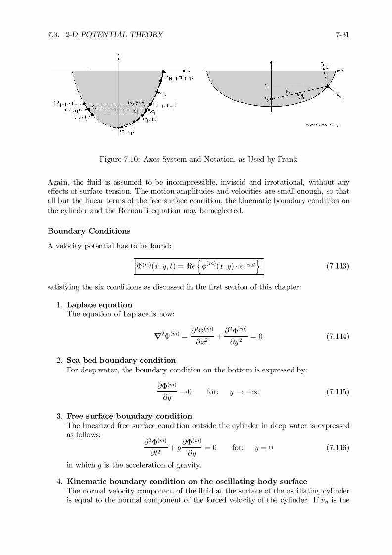
7.3. 2-D POTENTIAL THEORY 7-31
Figure 7.10: Axes System and Notation, as Used by Frank
Again, the ‡uid is assumed to be incompressible, inviscid and irrotational, without anye¤ects of surface tension. The motion amplitudes and velocities are small enough, so thatall but the linear terms of the free surface condition, the kinematic boundary condition onthe cylinder and the Bernoulli equation may be neglected.
Boundary Conditions
A velocity potential has to be found:
¯¯©(m)(x; y; t) = <e
nÁ(m)(x; y) ¢ e¡i!t
o¯¯ (7.113)
satisfying the six conditions as discussed in the …rst section of this chapter:
1. Laplace equationThe equation of Laplace is now:
r2©(m) =@2©(m)
@x2+@2©(m)
@y2= 0 (7.114)
2. Sea bed boundary conditionFor deep water, the boundary condition on the bottom is expressed by:
@©(m)
@y!0 for: y ! ¡1 (7.115)
3. Free surface boundary conditionThe linearized free surface condition outside the cylinder in deep water is expressedas follows:
@2©(m)
@t2+ g
@©(m)
@y= 0 for: y = 0 (7.116)
in which g is the acceleration of gravity.
4. Kinematic boundary condition on the oscillating body surfaceThe normal velocity component of the ‡uid at the surface of the oscillating cylinderis equal to the normal component of the forced velocity of the cylinder. If vn is the
7-32 CHAPTER 7. POTENTIAL COEFFICIENTS
component of the forced velocity of the cylinder in the direction of the outgoing unitnormal vector n, then the kinematic boundary condition has to be satis…ed at themean position of the cylindrical surface:
~n ¢ ~r©(m) = vn (7.117)
5. Radiation conditionAt a large distance from the cylinder the disturbed surface of the ‡uid has to takethe form of a regular progressive outgoing gravity wave.
6. Symmetric or anti-symmetric conditionBecause both the sway and the roll motion are anti-symmetric and the heave motionis symmetrical, these velocity potentials have the following relation:
sway : ©(2)(¡x; y) = ¡©(2)(+x; y)heave : ©(3)(¡x; y) = +©(3)(+x; y)
roll : ©(4)(¡x; y) = ¡©(4)(+x; y) (7.118)
Velocity Potentials
A potential function, based on pulsating point-sources and satisfying these six conditions,has been given by [Frank, 1967]. Based on earlier work of [Wehausen and Laitone, 1960],the complex potential at z of a pulsating point-source of unit strength at the point ³ inthe lower half plane, as shown in …gure 7.10, was given by Frank as:
G¤(z; ³; t) =1
2¼
8<:ln(z ¡ ³)¡ ln(z ¡b³) + 2PV
1Z
0
e¡ik(z¡b³)
º ¡ k dk
9=; ¢ cos!t
¡ne¡iº(z¡
b³)o
¢ sin!t (7.119)
where:
z = x+ iy ³ = » + i´ b³ = » ¡ i´ (7.120)
In here, ³ is de…ned in the lower half plane and b³ in the upper half plane (mirrored), while
º = !2=g is the wave number in deep water and PV1R0
e¡ik(z¡b³)º¡k dk is a principle value
integral with a variable k. These somewhat unconventional notations come from Frank’sreport and are maintained here.With this, the real part of the point-source potential is de…ned by:
H(x; y; »; ´; t) = <e fG¤(z; ³; t)g (7.121)
The space and time dependent source potential term, G¤(z; ³; t), is now written in terms ofa separate space dependent potential, G(z; ³), multiplied by an oscillatory motion, e¡i!t:
G¤(z; ³; t) = G(z; ³) ¢ e¡i!t (7.122)
7.3. 2-D POTENTIAL THEORY 7-33
With this space dependent potential:
G(z; ³) =1
2¼¢ <e
8<:ln(z ¡ ³)¡ ln(z ¡b³) + 2
1Z
0
e¡ik(z¡b³)
º ¡ k dk
9=;
¡i¢ <ene¡iº(z¡
b³)o
(7.123)
two expressions for the point-source potential, satisfying all six boundary conditions, arefound:
H (x; y; »; ´;t ) = <e©G(z; ³) ¢ e¡i!tª
H(x; y; »; ´; t¡ ¼
2!) = <e
©i ¢G(z; ³) ¢ e¡i!t
ª(7.124)
Since the problem is linear, a superposition of these two valid expressions for the point-source potential H results in the velocity potential:
¯¯¯©(m)(x; y; t) = <e
8<:
Z
C0
Q(s) ¢G(z; ³) ¢ e¡i!t ¢ ds
9=;
¯¯¯ (7.125)
where C0 is the submerged contour of the cylindrical cross section at its mean or restposition and Q(s) represents the complex source density as a function of the position alongC0.Application of the kinematic boundary condition on the oscillating cylinder at z yields:
<e
8<:(~n ¢ ~r)
Z
C0
Q(s) ¢G(z; ³) ¢ ds
9=; = 0
=m
8<:(~n ¢ ~r)
Z
C0
Q(s) ¢G(z; ³) ¢ ds
9=; = A(m) ¢ ! ¢ n(m) (7.126)
where A(m) denotes the amplitude of oscillation and n(m) the direction cosine of the normalvelocity at z on the cylinder. Both A(m) and n(m) depend on the mode of motion of thecylinder, as will be shown below.The fact that Q(s) is complex implies that the last two equations represent a set of coupledintegral equations for the real functions <efQ(s)g and =mfQ(s)g. Frank describes theevaluation of the integrals in his report; special attention is focussed there on the singularityfor z = ³ and k = º.
Solution
Select N + 1 points (»i; ´i) which lie on C0 in the fourth quadrant. Connect these N +1points by successive straight lines. N straight line segments are obtained which, togetherwith their re‡ected images in the third quadrant, yield an approximation to the givencontour as shown in …gure 7.10. The coordinates, length and angle associated with thej-th segment are identi…ed by the subscript j, whereas the corresponding quantities for the
7-34 CHAPTER 7. POTENTIAL COEFFICIENTS
re‡ected image in the third quadrant are denoted by the subscript ¡j, so that by symmetry»¡j = ¡»j and ´¡j = ¡´j for 1 · j · N + 1.Potentials and pressures are to be evaluated at the midpoint of each segment and for1 · i · N the coordinates of the midpoint of the i-th segment are:
xi =»i + »i+1
2and yi =
´i + ´i+12
(7.127)
The length of the i-th segment and the angle between by this segment and the positive xaxis are:
jsij =q¡»i+1 ¡ »i
¢2+
¡´i+1 ¡ ´i
¢2®i = arctan
½´i+1¡ ´ i»i+1¡ »i
¾(7.128)
The outgoing unit vector normal to the cross section at the i-th midpoint (xi; yi) is:
~ni =~i sin®i ¡ ~j cos®i (7.129)
where ~i and ~j are unit vectors in the x- and y-directions, respectively.
The cylinder is forced into a simple harmonic motion with radian frequency !, accordingto the displacement equation:
S(m) = A(m) ¢ cos!t (7.130)
for m = 2, 3 or 4, corresponding to sway, heave or roll, respectively. The rolling motionsare about an axis through a point (0; y0) in the symmetry plane of the cylinder.In the translational modes, any point on the cylinder moves with the velocity:
sway: ~v(2) = ¡~i A(2)! sin!theave: ~v(3) = ¡~j A(3)! sin!t (7.131)
The rolling motion is illustrated in …gure 7.10. Considering a point (xi; yi) on C0, aninspection of this …gure yields:
Ri =
qxi2 + (yi ¡ y0)2 and µi = arctan
½yi ¡ y0xi
¾
= arcsin
½yi ¡ y0Ri
¾
= arccos
½xiRi
¾(7.132)
Therefore, by elementary two-dimensional kinematics, the unit vector in the direction µ is:
~¿ i = ¡~i sin µi + ~j cos µi= ¡yi ¡ y0
Ri~i +
xiRi~j (7.133)
so that:
roll: ~v(4) = RiS(4)~¿ i
= !A(4)n(yi ¡ y0)~i¡ xi~j
osin!t (7.134)
7.3. 2-D POTENTIAL THEORY 7-35
The normal components of the velocity vi(m) = ~ni ¢~v (m) at the midpoint of the i-th segment(xi; yi) are:
sway: vi(2) = ¡!A(2) sin ®i sin !t
heave: vi(3) = +!A(3) cos®i sin!t
roll: vi(4) = +!A(4) f(yi ¡ y0) sin ®i + xi cos®ig sin!t (7.135)
De…ning:
ni(m) =
vi(m)
A(m)! sin!t(7.136)
then, consistent with the previously mentioned notation, the direction cosines for the threemodes of motion are:
sway: ni(2) = + sin ®i
heave: ni(3) = ¡ cos®iroll: ni
(4) = + (yi ¡ y0) sin®i + xi cos®i (7.137)
These equations illustrate that heaving is symmetrical: n¡i(3) = ni(3). Swaying and rolling,however are antisymmetric modes: n¡i(2) = ¡ni(2) and n¡i(4) = ¡ni(4).The set of two coupled integral equations for the real functions <efQ(s)g and =mfQ(s)g,given before, are applied at the midpoints of each of the N segments. It is assumed thatover an individual segment the complex source strength Q(s) remains constant, althoughit varies from segment to segment. With these stipulations, the set of coupled integralequations becomes a set of 2N linear algebraic equations in the unknowns:
<e©Q(m) ¢ (sj)
ª= Qj
(m)
=m©Q(m) ¢ (sj)
ª= QN+j
(m) (7.138)
Thus, for i = 1, 2, ....., N :
+NX
j=1
nQj
(m) ¢ Iij(m)o+
NX
j=1
nQN+j
(m) ¢ Jij(m)o= 0
¡NX
j=1
nQj
(m) ¢ Jij(m)o+
NX
j=1
nQN+j
(m) ¢ Iij(m)o= ! ¢ A(m) ¢ ni(m) (7.139)
where the superscript (m) in these 2N2 equations denotes the mode of motion.The in‡uence coe¢cients Iij(m) and Jij(m) and the potential ©(m)(xi; yi; t) have been eval-uated by [Frank, 1967]. The resulting velocity potential consists of a term in-phase withthe displacement and a term in-phase with the velocity.The hydrodynamic pressure at (xi; yi) along the cylinder is obtained from the velocitypotential by means of the linearized Bernoulli equation:
p(m)(xi; yi; !; t) = ¡½ ¢ @©(m)
@t(xi; yi; !; t) (7.140)
Since:
p(m)(xi; yi; !; t) = pa(m)(xi; yi;!) ¢ cos!t
+pv(m)(xi; yi;!) ¢ sin!t (7.141)
7-36 CHAPTER 7. POTENTIAL COEFFICIENTS
where pa(m) and pv(m) are the hydrodynamic pressures in-phase with the displacement andin-phase with the velocity, respectively.As indicated by the previous expressions, the potential as well as the pressure is a functionof the oscillation frequency !. The hydrodynamic force or moment per unit length ofthe cylinder, necessary to sustain the oscillations, is the integral of p(m) ¢ n(m) over thesubmerged contour of the cross section C0. It is assumed that the pressure at the i-thmidpoint is the mean pressure for the i-th segment, so that the integration reduces to asummation, so that:
¯¯¯M
(m)(!) = 2NX
i=1
pa(m)(xi; yi;!) ¢ ni(m) ¢ jsij¯¯¯
¯¯¯N
(m)(!) = 2NX
i=1
pv(m)(xi; yi;!) ¢ ni(m) ¢ jsij¯¯¯ (7.142)
for the potential inertia and damping forces or moments, respectively.
7.3.5 Comparative Results
Figure 7.11 compares the calculated coe¢cients for an amidships cross section of a containervessel with the three previous methods:
- Ursell-Tasai’s method with 2-parameter Lewis conformal mapping.
- Ursell-Tasai’s method with 10-parameter close-…t conformal mapping.
- Frank’s pulsating source method.
With the exception of the roll motions, the three results are very close. The roll motion de-viation, predicted with the Lewis conformal mapping method, is caused by the descriptionof the ”bilge” by the simple Lewis transformation, as can be seen in …gure 7.8.A disadvantage of Frank’s method can be the large computing time, when compared withUrsell-Tasai’s method. Generally, it is advised to use Ursell-Tasai’s method with 10 para-meter close-…t conformal mapping. For submerged sections, bulbous sections and sectionswith an area coe¢cient, ¾s, less than 0.5, Frank’s pulsating source method should be used.
7.4 3-D Potential Theory
The previous main section of this chapter has discussed the potential theory for two-dimensional (plane) shapes. Floating bodies are obviously three-dimensional and it can beappropriate therefore to attempt to determine their potential theory coe¢cients directlyin three dimensions, similar to what Frank did in the two-dimensional case. Just as earlierin this chapter, the presentation here is intended to provide only a bit of insight intothe derivation path being followed. The path and the result is more important than thederivation details.Three-dimensional methods to evaluate the hydrodynamic loads and motions of …xed or(with zero mean forward speed) ‡oating structures in waves have been developed based
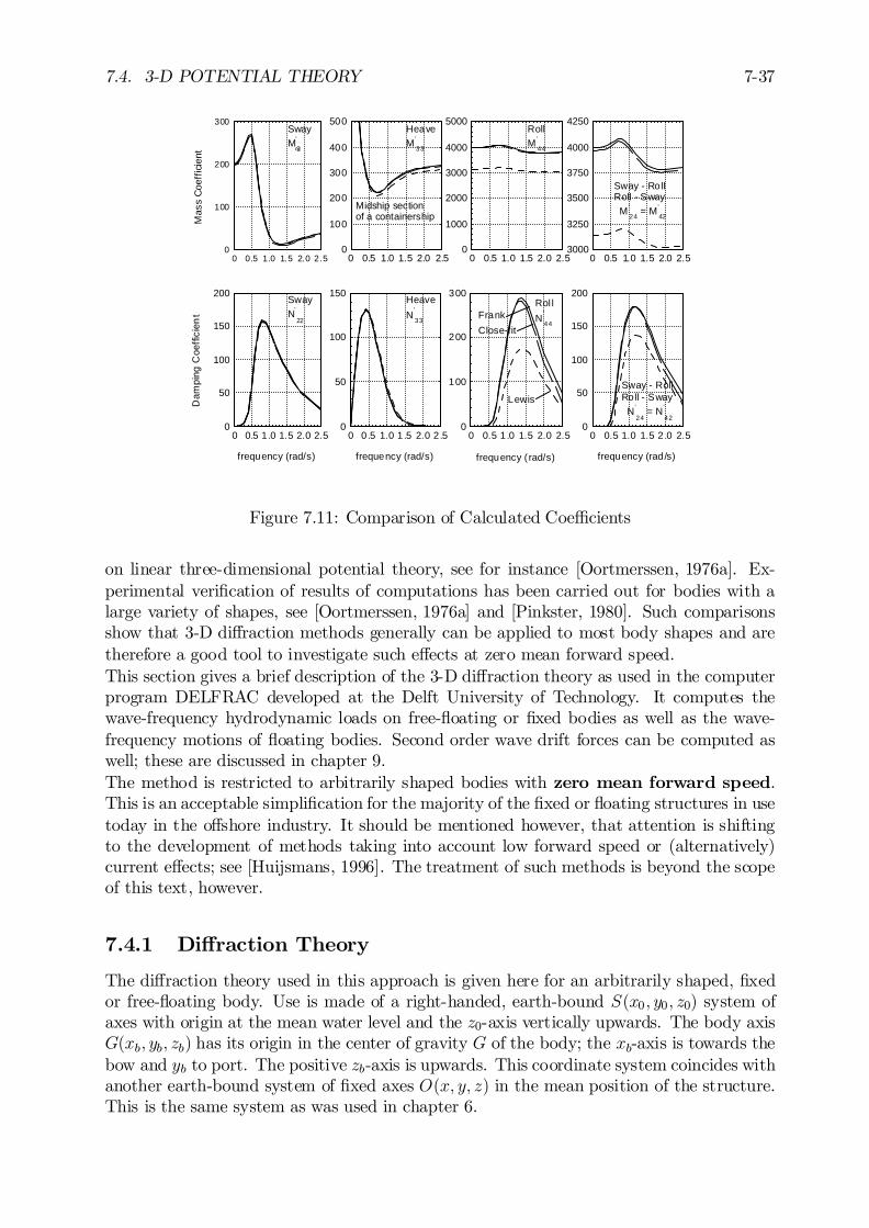
7.4. 3-D POTENTIAL THEORY 7-37
0
100
200
300
400
500
0 0.5 1.0 1.5 2.0 2.5
HeaveM '
33
0
1000
2000
3000
4000
5000
0 0.5 1.0 1.5 2.0 2.5
RollM '
44
0
50
100
150
0 0.5 1.0 1.5 2.0 2.5
HeaveN
'
33
frequency (rad/s)
0
50
100
150
200
0 0.5 1.0 1.5 2.0 2.5
SwayN'
22
frequency (rad/s)
Dam
ping
Coe
ffici
ent
0
100
200
300
0 0.5 1.0 1.5 2.0 2.5
Midship sectionof a containership
SwayM'
22
Mas
s C
oeff
icie
nt
0
50
100
150
200
0 0.5 1.0 1.5 2.0 2.5
Sway - RollRoll - Sway N '
24 = N '
42
frequency (rad/s)
3000
3250
3500
3750
4000
4250
0 0.5 1.0 1.5 2.0 2.5
Sway - RollRoll - Sway M '
24 = M '
42
0
100
200
300
0 0.5 1.0 1.5 2.0 2.5
Close-fit
Lewis
FrankRol lN
'
44
frequency ( rad/s)
Figure 7.11: Comparison of Calculated Coe¢cients
on linear three-dimensional potential theory, see for instance [Oortmerssen, 1976a]. Ex-perimental veri…cation of results of computations has been carried out for bodies with alarge variety of shapes, see [Oortmerssen, 1976a] and [Pinkster, 1980]. Such comparisonsshow that 3-D di¤raction methods generally can be applied to most body shapes and aretherefore a good tool to investigate such e¤ects at zero mean forward speed.This section gives a brief description of the 3-D di¤raction theory as used in the computerprogram DELFRAC developed at the Delft University of Technology. It computes thewave-frequency hydrodynamic loads on free-‡oating or …xed bodies as well as the wave-frequency motions of ‡oating bodies. Second order wave drift forces can be computed aswell; these are discussed in chapter 9.The method is restricted to arbitrarily shaped bodies with zero mean forward speed.This is an acceptable simpli…cation for the majority of the …xed or ‡oating structures in usetoday in the o¤shore industry. It should be mentioned however, that attention is shiftingto the development of methods taking into account low forward speed or (alternatively)current e¤ects; see [Huijsmans, 1996]. The treatment of such methods is beyond the scopeof this text, however.
7.4.1 Di¤raction Theory
The di¤raction theory used in this approach is given here for an arbitrarily shaped, …xedor free-‡oating body. Use is made of a right-handed, earth-bound S(x0; y0; z0) system ofaxes with origin at the mean water level and the z0-axis vertically upwards. The body axisG(xb; yb; zb) has its origin in the center of gravity G of the body; the xb-axis is towards thebow and yb to port. The positive zb-axis is upwards. This coordinate system coincides withanother earth-bound system of …xed axes O(x; y; z) in the mean position of the structure.This is the same system as was used in chapter 6.

7-38 CHAPTER 7. POTENTIAL COEFFICIENTS
The wave elevation and all potentials are referenced to the …xed O(x; y; z) system of axes.Phase shifts of body motions are referenced to the undisturbed wave elevation at the centerof gravity (G= O) of the body; even though no wave can be measured there.According to linear potential theory, the potential of a ‡oating body is a superposition ofthe potentials due to the undisturbed incoming wave ©w, the potential due to the di¤ractionof the undisturbed incoming wave on the …xed body ©d and the radiation potentials dueto the six body motions ©j: ¯
¯¯© =
6X
j=1
©j + ©w +©d
¯¯¯ (7.143)
Again, the ‡uid is assumed to be incompressible, inviscid and irrotational, without anye¤ects of surface tension. The motion amplitudes and velocities are small enough, so thatall but the linear terms of the free surface condition, the kinematic boundary condition onthe body and the Bernoulli equation may be neglected.
The potentials have to satisfy the same boundary conditions, as discussed before:
1. Laplace equationThe continuity condition or Laplace equation:
@2©
@x2+@2©
@y2+@2©
@z2= 0 (7.144)
holds in the ‡uid domain.
2. Sea bed boundary conditionAt the sea bed:
@©
@z= 0 with: z = ¡ho (7.145)
in which ho is the distance from the origin of the earth-bound coordinate system,O(x; y; z), to the sea bed. Note that, in contrast to the earlier theory, this treatmentis for water with a …nite depth.
3. Free surface boundary conditionAt the mean free surface:
g@©
@z+@2©
@t2= 0 (7.146)
4. Kinematic boundary condition on the oscillating body surfaceOn the wetted part of the oscillating hull of the structure (in its mean position):
@©
@n= ~v:~n (7.147)
in which ~v is the velocity of a point on the hull of the body and ~n is the normalvector of the hull, positive into the ‡uid.
5. Radiation conditionThe body motion and di¤raction potentials have to satisfy a radiation condition whichstates that at great distance from the body these potentials disappear. This conditionimposes a uniqueness which would not otherwise be present, see [Oortmerssen, 1976a].
7.4. 3-D POTENTIAL THEORY 7-39
6. Symmetric or anti-symmetric conditionIf, for instance for ships, both the sway and the roll motion of the ‡uid are anti-symmetric and the heave motion is symmetrical, the velocity potentials have thefollowing relation:
©(2)(¡x; y) = ¡©(2)(+x; y) for sway
©(3)(¡x; y) = +©(3)(+x; y) for heave (7.148)
©(4)(¡x; y) = ¡©(4)(+x; y) for roll
However, this symmetry condition has not to be used in DELFRAC necessarily,because this program is suitable for any hull form..
The free-surface condition follows from the assumptions that the pressure at the surface isconstant and that water particles do not pass through the free surface. The condition onthe wetted surface of the body assures the no-leak condition of the (oscillating) hull. Thecondition at the sea bed is also a no-leak condition.Up to now no speci…c wave conditions have been applied. The boundary conditions aregeneral and apply to all possible realizations of wave conditions. The theory is developedhere for a unidirectional regular wave. Just as in chapter 5, superposition can then be usedto study all sorts of irregular wave conditions - even those with directional spreading.In regular waves a linear potential ©, which is a function of the earth-…xed coordinatesand of time t, can be written as a product of a space-dependent term and a harmonictime-dependent term as follows:
j©(x; y; z; t) = Á(x; y; z) ¢ e¡i!tj (7.149)
The boundary conditions for the potential, ©, result in similar conditions for the spacedependent term, Á.
Note: Following [Tuck, 1970] a convenient formulation can be obtained by writing:
Á = ¡i!7X
j=0
Áj³j (7.150)
in which j = 0 represents the undisturbed incoming wave, j = 1; :::6 are associated witheach of the motion modes of the body and j = 7 represents the di¤racted wave.
The space-dependent part of the velocity potential Á0 - associated with an undisturbedlong-crested regular wave in water of constant depth h - is given by:
Á0 =³0g
!¢ coshk(ho + z)
coshkh¢ eik(xcos¹+y sin¹) (7.151)
in which:
³0 = amplitude of undisturbed wave (m)k = 2¼=¸ = wave number at shallow water (rad/m)¸ = wave length (m)¹ = wave direction (rad); zero for a wave travelling in the positive x-direction! = wave frequency (rad/s)ho = distance from the origin, O, of the earth-…xed axes to the sea bed (m)h = water depth (m)
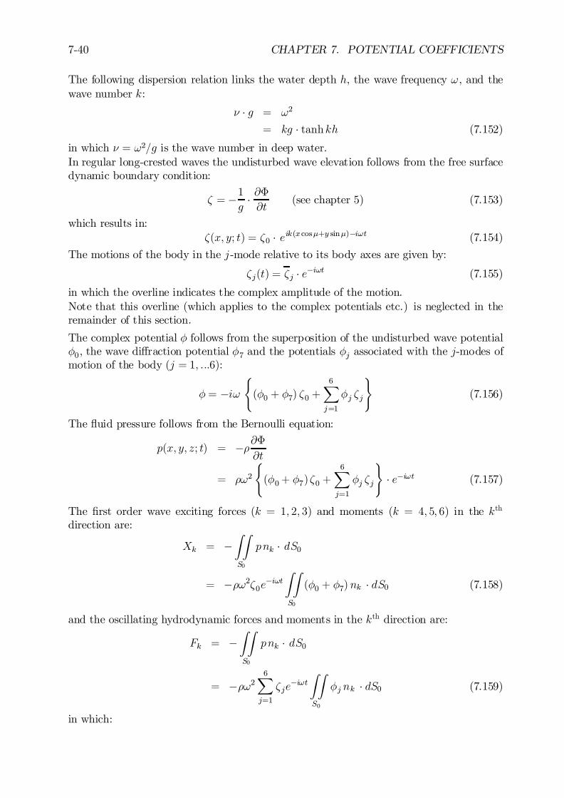
7-40 CHAPTER 7. POTENTIAL COEFFICIENTS
The following dispersion relation links the water depth h, the wave frequency !, and thewave number k:
º ¢ g = !2
= kg ¢ tanhkh (7.152)
in which º = !2=g is the wave number in deep water.In regular long-crested waves the undisturbed wave elevation follows from the free surfacedynamic boundary condition:
³ = ¡1g
¢ @©@t
(see chapter 5) (7.153)
which results in:³(x; y; t) = ³0 ¢ eik(xcos¹+y sin¹)¡i!t (7.154)
The motions of the body in the j-mode relative to its body axes are given by:
³j(t) = ³j ¢ e¡i!t (7.155)
in which the overline indicates the complex amplitude of the motion.Note that this overline (which applies to the complex potentials etc.) is neglected in theremainder of this section.
The complex potential Á follows from the superposition of the undisturbed wave potentialÁ0, the wave di¤raction potential Á7 and the potentials Áj associated with the j-modes ofmotion of the body (j = 1; :::6):
Á = ¡i!((Á0 + Á7) ³0 +
6X
j=1
Áj ³j
)(7.156)
The ‡uid pressure follows from the Bernoulli equation:
p(x; y; z; t) = ¡½@©@t
= ½!2
((Á0+ Á7)³0 +
6X
j=1
Áj ³j
)¢ e¡i!t (7.157)
The …rst order wave exciting forces (k = 1; 2; 3) and moments (k = 4; 5; 6) in the kth
direction are:
Xk = ¡ZZ
S0
pnk ¢ dS0
= ¡½!2³0e¡i!tZZ
S0
(Á0 + Á7) nk ¢ dS0 (7.158)
and the oscillating hydrodynamic forces and moments in the kth direction are:
Fk = ¡ZZ
S0
pnk ¢ dS0
= ¡½!26X
j=1
³je¡i!t
ZZ
S0
Áj nk ¢ dS0 (7.159)
in which:
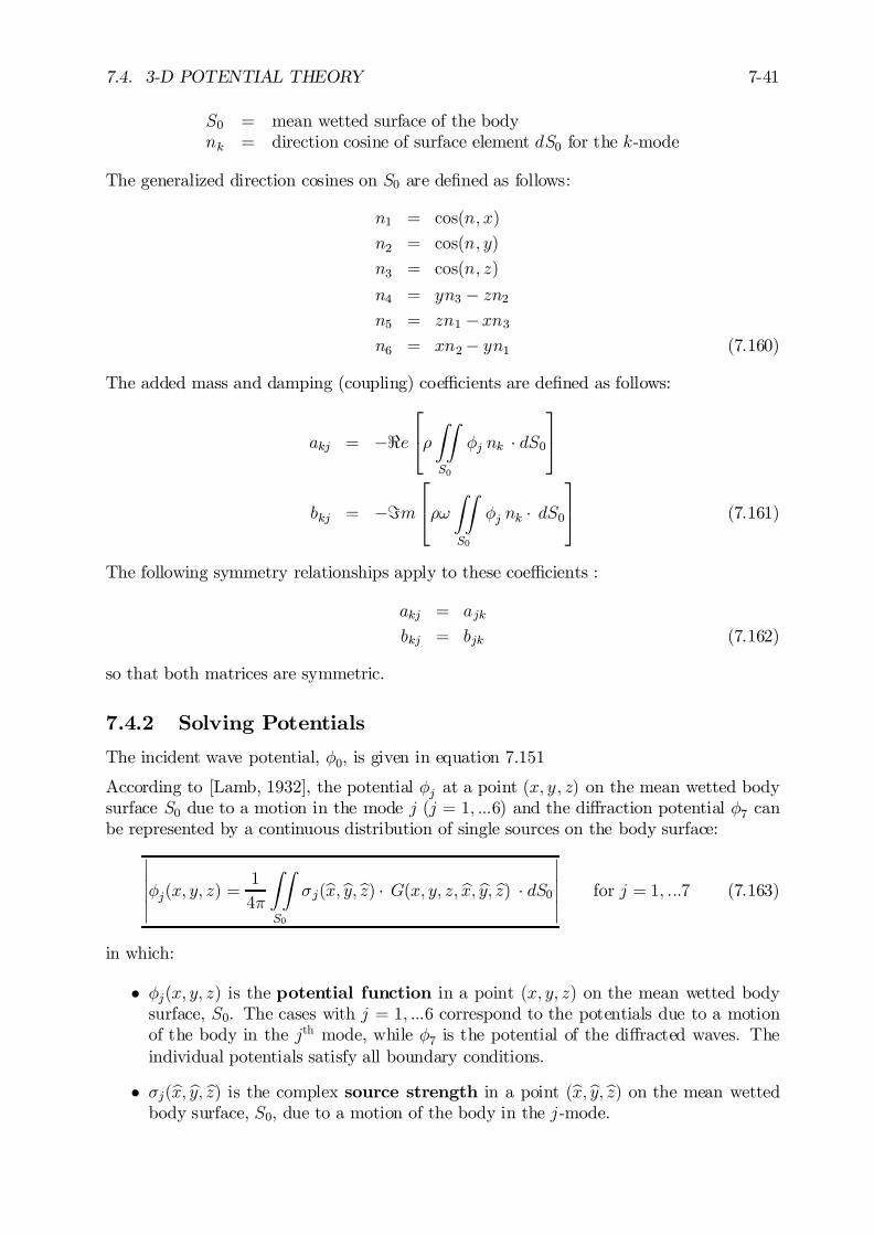
7.4. 3-D POTENTIAL THEORY 7-41
S0 = mean wetted surface of the bodynk = direction cosine of surface element dS0 for the k-mode
The generalized direction cosines on S0 are de…ned as follows:
n1 = cos(n; x)
n2 = cos(n; y)
n3 = cos(n; z)
n4 = yn3 ¡ zn2n5 = zn1 ¡xn3n6 = xn2¡ yn1 (7.160)
The added mass and damping (coupling) coe¢cients are de…ned as follows:
akj = ¡<e
24½
ZZ
S0
Áj nk ¢ dS0
35
bkj = ¡=m
24½!
ZZ
S0
Áj nk ¢ dS0
35 (7.161)
The following symmetry relationships apply to these coe¢cients :
akj = ajk
bkj = bjk (7.162)
so that both matrices are symmetric.
7.4.2 Solving Potentials
The incident wave potential, Á0, is given in equation 7.151
According to [Lamb, 1932], the potential Áj at a point (x; y; z) on the mean wetted bodysurface S0 due to a motion in the mode j (j = 1; :::6) and the di¤raction potential Á7 canbe represented by a continuous distribution of single sources on the body surface:
¯¯¯Áj(x; y; z) =
1
4¼
ZZ
S0
¾j(bx;by;bz) ¢ G(x; y; z; bx; by; bz) ¢ dS0
¯¯¯ for j = 1; :::7 (7.163)
in which:
² Áj(x; y; z) is the potential function in a point (x; y; z) on the mean wetted bodysurface, S0. The cases with j = 1; :::6 correspond to the potentials due to a motionof the body in the jth mode, while Á7 is the potential of the di¤racted waves. Theindividual potentials satisfy all boundary conditions.
² ¾j(bx; by; bz) is the complex source strength in a point (bx;by;bz) on the mean wettedbody surface, S0, due to a motion of the body in the j-mode.
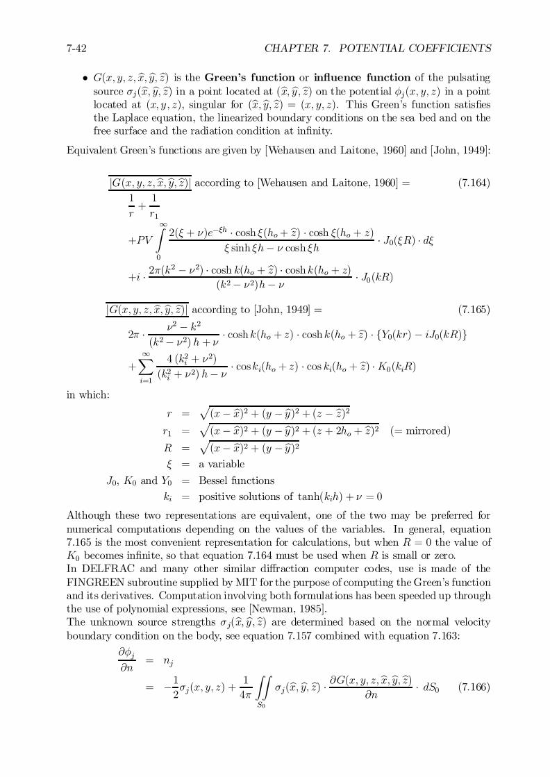
7-42 CHAPTER 7. POTENTIAL COEFFICIENTS
² G(x; y; z; bx; by; bz) is the Green’s function or in‡uence function of the pulsatingsource ¾j(bx; by; bz) in a point located at (bx; by;bz) on the potential Áj(x; y; z) in a pointlocated at (x; y; z), singular for (bx;by;bz) = (x; y; z). This Green’s function satis…esthe Laplace equation, the linearized boundary conditions on the sea bed and on thefree surface and the radiation condition at in…nity.
Equivalent Green’s functions are given by [Wehausen and Laitone, 1960] and [John, 1949]:
jG(x; y; z;bx;by;bz)j according to [Wehausen and Laitone, 1960] = (7.164)1
r+1
r1
+PV
1Z
0
2(» + º)e¡»h ¢ cosh »(ho+ bz) ¢ cosh »(ho + z)» sinh »h¡ º cosh »h ¢ J0(»R) ¢ d»
+i ¢ 2¼(k2 ¡ º2) ¢ cosh k(ho + bz) ¢ coshk(ho + z)
(k2¡ º2)h¡ º ¢ J0(kR)
jG(x; y; z; bx;by; bz)j according to [John, 1949] = (7.165)
2¼ ¢ º2 ¡ k2(k2¡ º2) h + º ¢ coshk(ho + z) ¢ coshk(ho + bz) ¢ fY0(kr) ¡ iJ0(kR)g
+1X
i=1
4 (k2i + º2)
(k2i + º2) h¡ º ¢ coski(ho + z) ¢ cos ki(ho + bz) ¢K0(kiR)
in which:
r =p(x¡ bx)2 + (y ¡ by)2 + (z ¡ bz)2
r1 =p(x¡ bx)2 + (y ¡ by)2 + (z + 2ho + bz)2 (= mirrored)
R =p(x¡ bx)2 + (y ¡ by)2
» = a variable
J0, K0 and Y0 = Bessel functions
ki = positive solutions of tanh(kih) + º = 0
Although these two representations are equivalent, one of the two may be preferred fornumerical computations depending on the values of the variables. In general, equation7.165 is the most convenient representation for calculations, but when R = 0 the value ofK0 becomes in…nite, so that equation 7.164 must be used when R is small or zero.In DELFRAC and many other similar di¤raction computer codes, use is made of theFINGREEN subroutine supplied by MIT for the purpose of computing the Green’s functionand its derivatives. Computation involving both formulations has been speeded up throughthe use of polynomial expressions, see [Newman, 1985].The unknown source strengths ¾j(bx; by;bz) are determined based on the normal velocityboundary condition on the body, see equation 7.157 combined with equation 7.163:
@Áj@n
= nj
= ¡12¾j(x; y; z) +
1
4¼
ZZ
S0
¾j(bx; by; bz) ¢ @G(x; y; z;bx;by;bz)@n
¢ dS0 (7.166)

7.4. 3-D POTENTIAL THEORY 7-43
In the above equations, the operator @=@n signi…es the gradient in the direction of thenormal to the surface of the body. For the solution of the motion potentials Áj, the right-hand side of the above equation 7.166 is given by the direction cosines de…ned by equation7.160.
For the solution of the di¤raction potential Á7 (restrained body), the right-hand side isgiven by:
n7 =@Á7@n
= ¡@Á0@n
(7.167)
Solving the integral equation 7.166 results in the unknown source strengths. Substitutionof these in equation 7.162 and in equation 7.159 yields the added mass and dampingcoe¢cients and the wave forces respectively.
Finally the motions ³j are determined from the solution of the following coupled equationsof motion for six degrees of freedom:
¯¯¯6X
j=1
f¡!2(mkj + akj)¡ i!bkj + ckjg ¢ ³j = Xk¯¯¯ for k = 1; :::6 (7.168)
with:
mkj = inertia matrix of the body for inertia coupling in the k-modefor acceleration in the j-mode
akj = added mass matrix for the force on the body in the k-modedue to acceleration of the body in the j-mode
bkj = damping matrix for the force on the body in the k-modedue to velocity of the body in the j-mode
ckj = spring matrix for the force on the body in the k-modedue to motion of the body in the j-mode
Xk = wave force on the body in the k-mode
The bkj and ckj matrices may contain contributions arising from mechanical damping de-vices and springs or even a mooring system.
7.4.3 Numerical Aspects
By discretizing the mean wetted surface of a body into N panels, on which the sourcestrengths are homogeneously distributed, the following discretized form of equation 7.166is obtained:
¡12¾mj +
1
4¼
NX
n=1
¾nj@Gmn@n
4Sn = nmj for m = 1; :::N n 6= m (7.169)
The normal velocity requirement can only be met at one point for each panel into whichthe mean wetted surface of the hull is divided. It is customary to chose the centroid of thepanel. Such points are known as collocation points; see appendix D.
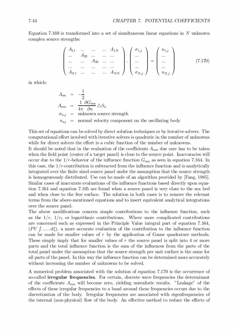
7-44 CHAPTER 7. POTENTIAL COEFFICIENTS
Equation 7.169 is transformed into a set of simultaneous linear equations in N unknowncomplex source strengths:
0BBBB@
A11 ::: ::: ::: A1N::: A22 ::: ::: :::::: ::: A33 ::: :::::: ::: ::: ::: :::AN1 ::: ::: ::: ANN
1CCCCA:
0BBBB@
¾1;j:::::::::¾N;j
1CCCCA=
0BBBB@
n1;j:::::::::nN;j
1CCCCA
(7.170)
in which:
Ann = ¡12
Anm =1
4¼
@Gmn@n
4Sn¾n;j = unknown source strength
nnj = normal velocity component on the oscillating body
This set of equations can be solved by direct solution techniques or by iterative solvers. Thecomputational e¤ort involved with iterative solvers is quadratic in the number of unknownswhile for direct solvers the e¤ort is a cubic function of the number of unknowns.It should be noted that in the evaluation of the coe¢cients Anm due care has to be takenwhen the …eld point (center of a target panel) is close to the source point. Inaccuracies willoccur due to the 1=r-behavior of the in‡uence function Gmn as seen in equation 7.164. Inthis case, the 1=r-contribution is subtracted from the in‡uence function and is analyticallyintegrated over the …nite sized source panel under the assumption that the source strengthis homogeneously distributed. Use can be made of an algorithm provided by [Fang, 1985].Similar cases of inaccurate evaluations of the in‡uence functions based directly upon equa-tion 7.164 and equation 7.165 are found when a source panel is very close to the sea bedand when close to the free surface. The solution in both cases is to remove the relevantterms from the above-mentioned equations and to insert equivalent analytical integrationsover the source panel.The above modi…cations concern simple contributions to the in‡uence function, suchas the 1=r, 1=r1 or logarithmic contributions. Where more complicated contributionsare concerned such as expressed in the Principle Value integral part of equation 7.164,(PV
R:::::: d»), a more accurate evaluation of the contribution to the in‡uence function
can be made for smaller values of r by the application of Gauss quadrature methods.These simply imply that for smaller values of r the source panel is split into 4 or moreparts and the total in‡uence function is the sum of the in‡uences from the parts of thetotal panel under the assumption that the source strength per unit surface is the same forall parts of the panel. In this way the in‡uence function can be determined more accuratelywithout increasing the number of unknowns to be solved.
A numerical problem associated with the solution of equation 7.170 is the occurrence ofso-called irregular frequencies. For certain, discrete wave frequencies the determinantof the coe¢cients Amn will become zero, yielding unrealistic results. ”Leakage” of thee¤ects of these irregular frequencies to a band around these frequencies occurs due to thediscretization of the body. Irregular frequencies are associated with eigenfrequencies ofthe internal (non-physical) ‡ow of the body. An e¤ective method to reduce the e¤ects of
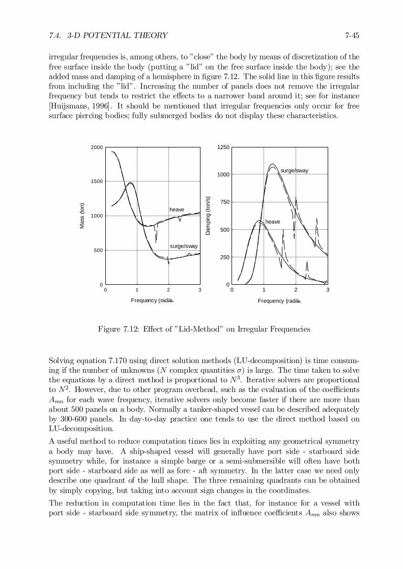
7.4. 3-D POTENTIAL THEORY 7-45
irregular frequencies is, among others, to ”close” the body by means of discretization of thefree surface inside the body (putting a ”lid” on the free surface inside the body); see theadded mass and damping of a hemisphere in …gure 7.12. The solid line in this …gure resultsfrom including the ”lid”. Increasing the number of panels does not remove the irregularfrequency but tends to restrict the e¤ects to a narrower band around it; see for instance[Huijsmans, 1996]. It should be mentioned that irregular frequencies only occur for freesurface piercing bodies; fully submerged bodies do not display these characteristics.
0
500
1000
1500
2000
0 1 2 3
heave
surge/sway
Frequency (rad/s)
Mas
s (to
n)
0
250
500
750
1000
1250
0 1 2 3
heave
surge/sway
Frequency (rad/s)
Dam
ping
(to
n/s)
Figure 7.12: E¤ect of ”Lid-Method” on Irregular Frequencies
Solving equation 7.170 using direct solution methods (LU-decomposition) is time consum-ing if the number of unknowns (N complex quantities ¾) is large. The time taken to solvethe equations by a direct method is proportional to N3. Iterative solvers are proportionalto N2. However, due to other program overhead, such as the evaluation of the coe¢cientsAmn for each wave frequency, iterative solvers only become faster if there are more thanabout 500 panels on a body. Normally a tanker-shaped vessel can be described adequatelyby 300-600 panels. In day-to-day practice one tends to use the direct method based onLU-decomposition.
A useful method to reduce computation times lies in exploiting any geometrical symmetrya body may have. A ship-shaped vessel will generally have port side - starboard sidesymmetry while, for instance a simple barge or a semi-submersible will often have bothport side - starboard side as well as fore - aft symmetry. In the latter case we need onlydescribe one quadrant of the hull shape. The three remaining quadrants can be obtainedby simply copying, but taking into account sign changes in the coordinates.
The reduction in computation time lies in the fact that, for instance for a vessel withport side - starboard side symmetry, the matrix of in‡uence coe¢cients Amn also shows
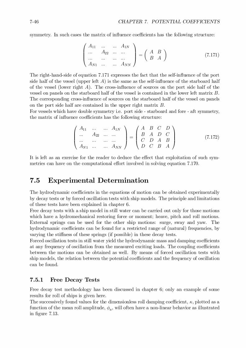
7-46 CHAPTER 7. POTENTIAL COEFFICIENTS
symmetry. In such cases the matrix of in‡uence coe¢cients has the following structure:
0BB@
A11 ::: ::: A1N::: A22 ::: :::::: ::: ::: :::AN1 ::: ::: ANN
1CCA =
µA BB A
¶(7.171)
The right-hand-side of equation 7.171 expresses the fact that the self-in‡uence of the portside half of the vessel (upper left A) is the same as the self-in‡uence of the starboard halfof the vessel (lower right A). The cross-in‡uence of sources on the port side half of thevessel on panels on the starboard half of the vessel is contained in the lower left matrix B.The corresponding cross-in‡uence of sources on the starboard half of the vessel on panelson the port side half are contained in the upper right matrix B.For vessels which have double symmetry i.e. port side - starboard and fore - aft symmetry,the matrix of in‡uence coe¢cients has the following structure:
0BB@
A11 ::: ::: A1N::: A22 ::: :::::: ::: ::: :::AN1 ::: ::: ANN
1CCA =
0BB@
A B C DB A D CC D A BD C B A
1CCA (7.172)
It is left as an exercise for the reader to deduce the e¤ect that exploitation of such sym-metries can have on the computational e¤ort involved in solving equation 7.170.
7.5 Experimental Determination
The hydrodynamic coe¢cients in the equations of motion can be obtained experimentallyby decay tests or by forced oscillation tests with ship models. The principle and limitationsof these tests have been explained in chapter 6.Free decay tests with a ship model in still water can be carried out only for those motionswhich have a hydromechanical restoring force or moment; heave, pitch and roll motions.External springs can be used for the other ship motions: surge, sway and yaw. Thehydrodynamic coe¢cients can be found for a restricted range of (natural) frequencies, byvarying the sti¤ness of these springs (if possible) in these decay tests.Forced oscillation tests in still water yield the hydrodynamic mass and damping coe¢cientsat any frequency of oscillation from the measured exciting loads. The coupling coe¢cientsbetween the motions can be obtained as well. By means of forced oscillation tests withship models, the relation between the potential coe¢cients and the frequency of oscillationcan be found.
7.5.1 Free Decay Tests
Free decay test methodology has been discussed in chapter 6; only an example of someresults for roll of ships is given here.The successively found values for the dimensionless roll damping coe¢cient, ·, plotted as afunction of the mean roll amplitude, Áa, will often have a non-linear behavior as illustratedin …gure 7.13.
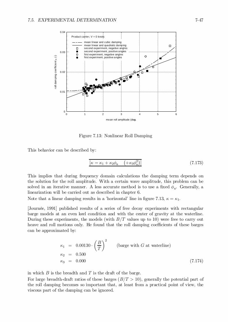
7.5. EXPERIMENTAL DETERMINATION 7-47
0
0.01
0.02
0.03
0.04
0 1 2 3 4 5 6
mean linear and cubic dampingmean linear and quadratic dampingsecond experiment, negative anglessecond experiment, positive anglesfirst experiment, negative anglesfirst experiment, positive angles
Product carrier, V = 0 knots
mean roll amplitude (deg)
roll
dam
ping
coe
ffici
ent
κ (
-)
Figure 7.13: Nonlinear Roll Damping
This behavior can be described by:
¯· = ·1 + ·2Áa
¡+·3Á
2a
¢¯(7.173)
This implies that during frequency domain calculations the damping term depends onthe solution for the roll amplitude. With a certain wave amplitude, this problem can besolved in an iterative manner. A less accurate method is to use a …xed Áa. Generally, alinearization will be carried out as described in chapter 6.Note that a linear damping results in a ’horizontal’ line in …gure 7.13, · = ·1.
[Journée, 1991] published results of a series of free decay experiments with rectangularbarge models at an even keel condition and with the center of gravity at the waterline.During these experiments, the models (with B=T values up to 10) were free to carry outheave and roll motions only. He found that the roll damping coe¢cients of these bargescan be approximated by:
·1 = 0:00130 ¢µB
T
¶2
(barge with G at waterline)
·2 = 0:500
·3 = 0:000 (7.174)
in which B is the breadth and T is the draft of the barge.For large breadth-draft ratios of these barges (B=T > 10), generally the potential part ofthe roll damping becomes so important that, at least from a practical point of view, theviscous part of the damping can be ignored.
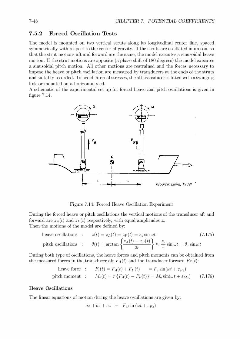
7-48 CHAPTER 7. POTENTIAL COEFFICIENTS
7.5.2 Forced Oscillation Tests
The model is mounted on two vertical struts along its longitudinal center line, spacedsymmetrically with respect to the center of gravity. If the struts are oscillated in unison, sothat the strut motions aft and forward are the same, the model executes a sinusoidal heavemotion. If the strut motions are opposite (a phase shift of 180 degrees) the model executesa sinusoidal pitch motion. All other motions are restrained and the forces necessary toimpose the heave or pitch oscillation are measured by transducers at the ends of the strutsand suitably recorded. To avoid internal stresses, the aft transducer is …tted with a swinginglink or mounted on a horizontal sled.A schematic of the experimental set-up for forced heave and pitch oscillations is given in…gure 7.14.
Figure 7.14: Forced Heave Oscillation Experiment
During the forced heave or pitch oscillations the vertical motions of the transducer aft andforward are zA(t) and zF (t) respectively, with equal amplitudes za.Then the motions of the model are de…ned by:
heave oscillations : z(t) = zA(t) = zF (t) = za sin !t (7.175)
pitch oscillations : µ(t) = arctan
½zA(t) ¡ zF(t)
2r
¾¼ zarsin !t = µa sin!t
During both type of oscillations, the heave forces and pitch moments can be obtained fromthe measured forces in the transducer aft FA(t) and the transducer forward FF (t):
heave force : Fz(t) = FA(t) +FF (t) = Fa sin(!t+ "Fz)
pitch moment : Mµ(t) = r fFA(t) ¡ FF(t)g = Ma sin(!t+ "Mz) (7.176)
Heave Oscillations
The linear equations of motion during the heave oscillations are given by:
aÄz + b _z + cz = Fa sin (!t+ "Fz)
7.5. EXPERIMENTAL DETERMINATION 7-49
dÄz + e _z + f z = Ma sin (!t+ "Mz) (7.177)
The components of the force and moment which are in-phase with the heave motion areassociated with the inertia and sti¤ness coe¢cients, while the out-of-phase components(also called in literature: quadrature components) are associated with damping.With:
z = za sin!t _z = za! cos!t Äz = ¡za!2 sin!t (7.178)
we obtain:
za¡¡a!2 + c
¢sin!t + zab! cos!t = Fa cos "Fz sin !t+ Fa sin "Fz cos!t
za¡¡d!2 + f
¢sin!t+ zae! cos!t = Ma cos "Mz sin!t+Ma sin "Mz cos!t(7.179)
which provides:
a = ½r + azz =c¡ Fa
zacos "Fz
!2with: c = czz = ½gAw
b = bzz =Fazasin "Fz
!
d = aµz =f ¡ Ma
zacos "Mz
!2with: f = cµz = ½gSw
e = bµz =Mazasin "Mz
!(7.180)
To obtain the sti¤ness coe¢cients c and f , use has to be made of Aw (area of the waterline)and Sw (…rst order moment of the waterline), which can be obtained from the geometry ofthe ship model.It is also possible to obtain the sti¤ness coe¢cients from static experiments:
Äz = 0 and _z = 0 provides: c =F
zand f =
M
z
Pitch Oscillations
The linear equations during the pitch oscillations are given by:
aĵ + b _µ + cµ = Fa sin (!t+ "Fµ)
dĵ + e _µ + f µ = Ma sin (!t+ "Mµ) (7.181)
The components of the force and moment which are in-phase with the pitch motion areassociated with the inertia and sti¤ness coe¢cients, while the out-of-phase components areassociated with damping.With:
µ = µa sin !t _µ = µa! cos!t ĵ = ¡µa!2 sin!t (7.182)
we obtain:
µa¡¡a!2 + c
¢sin!t + µab! cos!t = Fa cos"Fµ sin!t+Fa sin "Fµ cos!t
µa¡¡d!2 + f
¢sin !t+ µae! cos!t = Ma cos"Mµ sin!t+Ma sin "Mµ cos!t(7.183)
7-50 CHAPTER 7. POTENTIAL COEFFICIENTS
which provides:
a = azµ =c¡ Fa
µacos"Fµ
!2with: c = czµ = ½gSw
b = bzµ =Faµasin "Fµ
!
d = Iyy + aµµ =f ¡ Ma
µacos "Mµ
!2with: f = cµµ = ½grGML
e = bµµ =Ma
µasin "Mµ
!(7.184)
To obtain the sti¤ness coe¢cients c and f, use has been made of Sw (…rst order momentof the waterline) and GML (longitudinal metacentric height), which can be obtained fromthe geometry of the ship model.It is also possible to obtain the sti¤ness coe¢cients from static experiments:
ĵ = 0 and _µ = 0 provides: c =F
µand f =
M
µ(7.185)
Signal Processing
The in-phase and out-of-phase parts of the measured signal can be found easily from anintegration over an integer number n of periods T of the measure signals multiplied bycos!t and sin!t, respectively. This is in fact a …rst order Fourier analysis; see appendixC.For the heave oscillations, this results in:
Fa sin "Fz =2
nT
nTZ
0
(FA(t) +FF(t)) ¢ cos!t ¢ dt
Fa cos "Fz =2
nT
nTZ
0
(FA(t) +FF(t)) ¢ sin!t ¢ dt
Ma sin "Mz =2r
nT
nTZ
0
(FA(t) ¡ FF(t)) ¢ cos!t ¢ dt
Ma cos "Mz =2r
nT
nTZ
0
(FA(t) ¡ FF(t)) ¢ sin!t ¢ dt (7.186)
Similar expressions can be found for the pitch oscillations.
Equations of Motion
With the measured hydromechanical coe¢cients, the coupled linear equations of heave andpitch motions in still water are given by:
(½r + azz)Äz + bzz _z + czzz + azµÄµ + bzµ _µ + czµµ = 0
(Ixx + aµµ)ĵ + bµµ _µ + cµµµ + aµz Äz + bµz _z + cµzz = 0 (7.187)
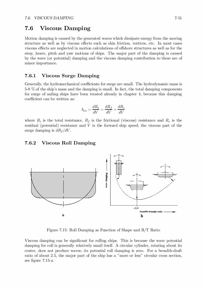
7.6. VISCOUS DAMPING 7-51
7.6 Viscous Damping
Motion damping is caused by the generated waves which dissipate energy from the movingstructure as well as by viscous e¤ects such as skin friction, vortices, etc. In most casesviscous e¤ects are neglected in motion calculations of o¤shore structures as well as for thesway, heave, pitch and yaw motions of ships. The major part of the damping is causedby the wave (or potential) damping and the viscous damping contribution to these are ofminor importance.
7.6.1 Viscous Surge Damping
Generally, the hydromechanical coe¢cients for surge are small. The hydrodynamic mass is5-8 % of the ship’s mass and the damping is small. In fact, the total damping componentsfor surge of sailing ships have been treated already in chapter 4, because this dampingcoe¢cient can be written as:
bxx =dRtdV
=dRfdV
+dRrdV
where Rt is the total resistance, Rf is the frictional (viscous) resistance and Rr is theresidual (potential) resistance and V is the forward ship speed; the viscous part of thesurge damping is dRf=dV .
7.6.2 Viscous Roll Damping
Figure 7.15: Roll Damping as Function of Shape and B/T Ratio
Viscous damping can be signi…cant for rolling ships. This is because the wave potentialdamping for roll is generally relatively small itself. A circular cylinder, rotating about itscenter, does not produce waves; its potential roll damping is zero. For a breadth-draftratio of about 2.5, the major part of the ship has a ”more or less” circular cross section,see …gure 7.15-a.
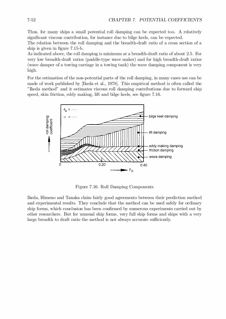
7-52 CHAPTER 7. POTENTIAL COEFFICIENTS
Thus, for many ships a small potential roll damping can be expected too. A relativelysigni…cant viscous contribution, for instance due to bilge keels, can be expected.The relation between the roll damping and the breadth-draft ratio of a cross section of aship is given in …gure 7.15-b.As indicated above, the roll damping is minimum at a breadth-draft ratio of about 2.5. Forvery low breadth-draft ratios (paddle-type wave maker) and for high breadth-draft ratios(wave damper of a towing carriage in a towing tank) the wave damping component is veryhigh.
For the estimation of the non-potential parts of the roll damping, in many cases use can bemade of work published by [Ikeda et al., 1978]. This empirical method is often called the”Ikeda method” and it estimates viscous roll damping contributions due to forward shipspeed, skin friction, eddy making, lift and bilge keels, see …gure 7.16.
Figure 7.16: Roll Damping Components
Ikeda, Himeno and Tanaka claim fairly good agreements between their prediction methodand experimental results. They conclude that the method can be used safely for ordinaryship forms, which conclusion has been con…rmed by numerous experiments carried out byother researchers. But for unusual ship forms, very full ship forms and ships with a verylarge breadth to draft ratio the method is not always accurate su¢ciently.
Chapter 8
FLOATING STRUCTURES INWAVES
8.1 Introduction
The (uncoupled) motions of a simple rigid body at zero forward speed have been discussedin chapter 6. Potential coe¢cients and their determination for more complex hull forms,such as those of ships and o¤shore structures, have been described in chapter 7.This chapter deals with the kinetics, the equations of motion for six degrees of freedomand some motion related phenomena for ships and o¤shore structures, partly including theforward speed e¤ect.
8.2 Kinetics
The total mass as well as its distribution over the body is considered to be constant withtime. For ships and other ‡oating structures, this assumption is normally valid during atime which is large relative to the period of the motions. This holds that small e¤ects,such as for instance a decreasing mass due to fuel consumption, can be ignored.The solid mass matrix of a ‡oating structure is given below.
Solid mass matrix: m =
0BBBBBB@
½r 0 0 0 0 00 ½r 0 0 0 00 0 ½r 0 0 00 0 0 Ixx 0 ¡Ixz0 0 0 0 Iyy 00 0 0 ¡Izx 0 Izz
1CCCCCCA
(8.1)
The moments of inertia here are often expressed in terms of the radii of inertia and thesolid mass of the structure. Since Archimedes law is valid for a ‡oating structure:
Ixx = kxx2 ¢ ½r
Iyy = kyy2 ¢ ½r
Izz = kzz2 ¢ ½r (8.2)
0J.M.J. Journée and W.W. Massie, ”OFFSHORE HYDROMECHANICS”, First Edition, January 2001,Delft University of Technology. For updates see web site: http://www.shipmotions.nl.
8-2 CHAPTER 8. FLOATING STRUCTURES IN WAVES
When the distribution of the solid mass of a ship is unknown, the radii of inertia can beapproximated by:
for ships:
8<:kxx t 0:30 ¢B to 0:40 ¢Bkyy t 0:22 ¢ L to 0:28 ¢ Lkzz t 0:22 ¢ L to 0:28 ¢ L
in which L is the length and B is the breadth of the ship; the (generally small) couplingterms, Ixz = Izx, are simply neglected.Bureau Veritas proposes for the gyradius in roll:
kxx = 0:289 ¢B ¢Ã1:0 +
µ2 ¢KGB
¶2!
(8.3)
in which KG is the height of the center of gravity, G, above the keel.For many ships without cargo on board (ballast condition), the mass is concentrated atthe ends (engine room aft and ballast water forward to avoid a large trim), while for shipswith cargo on board (full load condition) the - more or less amidships laden - cargo playsan important role. Thus, the radii of inertia, kyy and kzz, are usually smaller in the fullload condition than in the ballast condition for normal ships. Note that the longitudinalradius of gyration of a long homogeneous rectangular beam with a length L is equal to
about 0:29 ¢ L³=
p1=12 ¢L
´.
As already mentioned in chapter 6, the equations of motions of a rigid body in a space…xed coordinate system follow from Newton’s second law. The vector equations for thetranslations of and the rotations about the center of gravity are given respectively by:
¯¯~F = d
dt
³m~U
´¯¯ and
¯¯ ~M =
d
dt
³~H
´¯¯ (8.4)
in which:
~F = resulting external force acting in the center of gravitym = mass of the rigid body~U = instantaneous velocity of the center of gravity~M = resulting external moment acting about the center of gravity~H = instantaneous angular momentum about the center of gravityt = time
As mentioned in chapter 6 as well, two important assumptions are made for the loads inthe right hand side of these equations:
a. The so-called hydromechanical forces and moments are induced by the harmonicoscillations of the rigid body, moving in the undisturbed surface of the ‡uid.
b. The so-called wave exciting forces and moments are produced by waves comingin on the restrained body.
Since the system is linear, these loads are added to obtain the total loads. Thus, afterassuming small motions, symmetry of the body and that the x-, y- and z-axes are principal

8.3. COUPLED EQUATIONS OF MOTION 8-3
axes, one can write the following six motion equations for the ship:
Surge:d
dt(½r ¢ _x) = ½r ¢ Äx = Xh1 +Xw1
Sway:d
dt(½r ¢ _y) = ½r ¢ Äy = Xh2 +Xw2
Heave:d
dt(½r ¢ _z) = ½r ¢ Äz =Xh3 +Xw3
Roll:d
dt
³Ixx ¢ _Á¡ Ixz ¢ _Ã
´= Ixx ¢ ÄÁ ¡ Ixz ¢ ÄÃ =Xh4 +Xw4
Pitch:d
dt
³Iyy ¢ _µ
´= Ixx ¢ ĵ = Xh5 +Xw5
Yaw:d
dt
³Izz ¢ _Ã ¡ Izx ¢ _Á
´= Izz ¢ ÄÃ ¡ Izx ¢ ÄÁ = Xh6 +Xw6 (8.5)
in which:
½ = density of waterr = volume of displacement of the shipIij = solid mass moment of inertia of the shipXh1 , Xh2, Xh3 = hydromechanical forces in the x-, y- and z-directions respectivelyXh4 , Xh5, Xh6 = hydromechanical moments about the x-, y- and z-axes respectivelyXw1, Xw2, Xw3 = exciting wave forces in the x-, y- and z-directions respectivelyXw4, Xw5, Xw6 = exciting wave moments about the x-, y- and z-axes respectively
Note: in many applications, Ixz = Izx is not known or small; hence their terms are oftenomitted.
8.3 Coupled Equations of Motion
Once the mass of the ‡oating object and its distribution within that object are known, thecoupled equations of motion in 6 degrees of freedom in waves can be written.
8.3.1 General De…nition
Based on Newton’s second law, the general equations of motion are given by:
¯¯¯6X
j=1
mi;j ¢ Äxj = Fi¯¯¯ for: i = 1; :::6 (8.6)
in which:
mi;j = 6x6 matrix of solid mass and inertia of the bodyÄxj = acceleration of the body in direction jFi = sum of forces or moments acting in direction i
8-4 CHAPTER 8. FLOATING STRUCTURES IN WAVES
When de…ning a linear system, with simple harmonic wave exciting forces and momentsgiven by:
jFwi(!e; t) = Fwai(!e) ¢ cos (!et+ "Fi(!e))j (8.7)
the resulting simple harmonic motions are:
xj(!e; t) = xaj (!e) ¢ cos(!et)_xj(!e; t) = ¡!e ¢ xaj (!e) ¢ sin(!et)Äxj(!e; t) = ¡!2e ¢ xaj (!e) ¢ cos(!et) (8.8)
The hydromechanical forces and moments Fhi;j , acting on an oscillating object in stillwater, consist of:
- linear hydrodynamic reaction forces and moments expressed in terms with the hy-drodynamic mass and damping coe¢cients:
¡ai;j(!e) ¢ Äxj(!e; t)¡ bi;j(!e) ¢ _xj(!e; t) (8.9)
- linear hydrostatic restoring forces and moments expressed in a term with a springcoe¢cient:
¡ci;j ¢ xj(!e; t) (8.10)
With these expressions, the 6 equations of motion become:
6X
j=1
mi;j ¢ Äxj =6X
j=1
f¡ai;j(!e) ¢ Äxj(!e; t) ¡ bi;j(!e) ¢ _xj(!e; t) ¡ ci;j ¢ xj(!e; t)
+Fwai(!e) ¢ cos (!et+ "i(!e))gfor: i = 1; :::6 (8.11)
After ordering the terms, the general linear equations of motion for 6 degrees of freedomin the frequency domain are:
6X
j=1
f(mi;j + ai;j(!e)) ¢ Äxj(!e; t) + bi;j(!e) ¢ _xj(!e; t) + ci;j ¢ xj(!e; t)g
= Fwai(!e) ¢ cos(!et+ "i(!e))for: i = 1; :::6 (8.12)
The hydrodynamic coe¢cients, ai;j(!e) and bi;j(!e), and the exciting wave load compo-nents, Fwai(!e) and "i(!e), can be calculated with two- or three-dimensional techniquesgiven in chapter 7.
8.3.2 Motion Symmetry of Ships
Generally, a ship has a vertical-longitudinal plane of symmetry, so that its motions can besplit into symmetric and anti-symmetric components. Surge, heave and pitch motions aresymmetric motions, that is to say that a point to starboard has the same motion as themirrored point to port side. It is obvious that the remaining motions sway, roll and yaware anti-symmetric motions. Symmetric and anti-symmetric motions are not coupled; they

8.3. COUPLED EQUATIONS OF MOTION 8-5
don’t have any e¤ect on each other. For instance, a vertical force acting at the center ofgravity can cause surge, heave and pitch motions, but will not result in sway, roll or yawmotions.Because of this symmetry and anti-symmetry, two sets of three coupled equations of motioncan be distinguished for ships:
Surge : ½r ¢ Äx ¡Xh1 =Xw1Heave : ½r ¢ Äz ¡Xh3 =Xw3Pitch : Ixx ¢ ĵ ¡Xh5 =Xw5
9=; symmetric motions
Sway : ½r ¢ Äy ¡Xh2 =Xw2Roll : Ixx ¢ ÄÁ ¡Ixz ¢ ÄÃ ¡Xh4 =Xw4Yaw : Izz ¢ ÄÃ ¡Izx ¢ ÄÁ ¡Xh6 =Xw6
9=; anti-symmetric motions
The coupled surge, heave and pitch equations of motion are:
(½r + a11) ¢ Äx +b11 ¢ _x +c11 ¢ x+a13 ¢ Äz +b13 ¢ _z +c13 ¢ z+a15 ¢ ĵ +b15 ¢ _µ +c15 ¢ µ = Xw1 (surge)
a31 ¢ Äx +b31 ¢ _x +c31 ¢ x+(½r + a33) ¢ Äz +b33 ¢ _z +c33 ¢ z
+a35 ¢ ĵ +b35 ¢ _µ +c35 ¢ µ = Xw3 (heave)
a51 ¢ Äx +b51 ¢ _x +c51 ¢ x+a53 ¢ Äz +b53 ¢ _z +c53 ¢ z
+(+Iyy + a55) ¢ ĵ +b55 ¢ _µ +c55 ¢ µ = Xw5 (pitch)
9>>>>>>>>>>>>>>>>=>>>>>>>>>>>>>>>>;
symmetricmotions
The coupled sway, roll and yaw equations of motion are:
(½r + a22) ¢ Äy +b22 ¢ _y +c22 ¢ y+a24 ¢ ÄÁ +b24 ¢ _Á +c24 ¢ Á+a26 ¢ ÄÃ +b26 ¢ _Ã +c26 ¢ Ã =Xw2 (sway)
a42 ¢ Äy +b42 ¢ _y +c42 ¢ y+(+Ixx+ a44) ¢ ÄÁ +b44 ¢ _Á +c44 ¢ Á+(¡Ixz + a46) ¢ ÄÃ +b46 ¢ _Ã +c46 ¢ Ã =Xw4 (roll)
a62 ¢ Äy +b62 ¢ _y +c62 ¢ y+(¡Izx+ a64) ¢ ÄÁ +b64 ¢ _Á +c64 ¢ Á+(+Izz + a66) ¢ ÄÃ +b66 ¢ _Ã +c66 ¢ Ã =Xw6 (yaw)
9>>>>>>>>>>>>>>>>>=>>>>>>>>>>>>>>>>>;
anti-symmetricmotions
Note that this distinction between symmetric and anti-symmetric motions disappears whenthe ship is anchored. Then, for instance, the pitch motions can generate roll motions viathe anchor lines.
8.3.3 2-D Strip Theory
Strip theory is a computational method by which the forces on and motions of a three-dimensional ‡oating body can be determined using results from two-dimensional potential
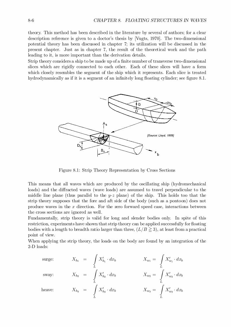
8-6 CHAPTER 8. FLOATING STRUCTURES IN WAVES
theory. This method has been described in the literature by several of authors; for a cleardescription reference is given to a doctor’s thesis by [Vugts, 1970]. The two-dimensionalpotential theory has been discussed in chapter 7; its utilization will be discussed in thepresent chapter. Just as in chapter 7, the result of the theoretical work and the pathleading to it, is more important than the derivation details.Strip theory considers a ship to be made up of a …nite number of transverse two-dimensionalslices which are rigidly connected to each other. Each of these slices will have a formwhich closely resembles the segment of the ship which it represents. Each slice is treatedhydrodynamically as if it is a segment of an in…nitely long ‡oating cylinder; see …gure 8.1.
Figure 8.1: Strip Theory Representation by Cross Sections
This means that all waves which are produced by the oscillating ship (hydromechanicalloads) and the di¤racted waves (wave loads) are assumed to travel perpendicular to themiddle line plane (thus parallel to the y-z plane) of the ship. This holds too that thestrip theory supposes that the fore and aft side of the body (such as a pontoon) does notproduce waves in the x direction. For the zero forward speed case, interactions betweenthe cross sections are ignored as well.Fundamentally, strip theory is valid for long and slender bodies only. In spite of thisrestriction, experiments have shown that strip theory can be applied successfully for ‡oatingbodies with a length to breadth ratio larger than three, (L=B = 3), at least from a practicalpoint of view.When applying the strip theory, the loads on the body are found by an integration of the2-D loads:
surge: Xh1 =
Z
L
X 0h1
¢ dxb Xw1 =
Z
L
X 0w1
¢ dxb
sway: Xh2 =
Z
L
X 0h2 ¢ dxb Xw2 =
Z
L
X 0w2 ¢ dxb
heave: Xh3 =
Z
L
X 0h3 ¢ dxb Xw3 =
Z
L
X 0w3 ¢ dxb

8.3. COUPLED EQUATIONS OF MOTION 8-7
roll: Xh4 =
Z
L
X 0h4
¢ dxb Xw4 =
Z
L
X 0w4
¢ dxb
pitch: Xh5 = ¡Z
L
X 0h3
¢ xb ¢ dxb Xw5 = ¡Z
L
X 0w3
¢ xb ¢ dxb
yaw: Xh6 =
Z
L
X 0h2 ¢ xb ¢ dxb Xw6 =
Z
L
X 0w2 ¢ xb ¢ dxb (8.13)
in which:
X 0hj
= sectional hydromechanical force or momentin direction j per unit ship length
X 0wj = sectional exciting wave force or moment
in direction j per unit ship length
The appearance of two-dimensional surge forces seems strange here. It is strange! A moreor less empirical method is used in program SEAWAY of [Journée, 1999] for the surgemotion, by de…ning an equivalent longitudinal cross section which is swaying. Then, the2-D hydrodynamic sway coe¢cients of this equivalent cross section are translated to 2-Dhydrodynamic surge coe¢cients by an empirical method based on theoretical results fromthree-dimensional calculations and these coe¢cients are used to determine 2-D loads. Inthis way, all sets of six surge loads can be treated in the same numerical way in programSEAWAY for the determination of the 3-D loads. Inaccuracies of the hydromechanical co-e¢cients of (slender) ships are of minor importance, because these coe¢cients are relativelysmall.Note how in the strip theory the pitch and yaw moments are derived from the 2-D heaveand sway forces, respectively, while the roll moments are obtained directly.The equations of motions are de…ned in the moving axis system with the origin at theaverage position of the center of gravity, G. All two-dimensional potential coe¢cientshave been de…ned so far in an axis system with the origin, O, in the water plane; thehydromechanical and exciting wave moments have to be corrected for the distance OG.
Potential Coe¢cients
As mentioned before, in strip theory calculations the two-dimensional sway, heave and rollcoe¢cients can be calculated by three methods which are summarized here; full details aregiven in chapter 7:
1. Ursell-Tasai’s Method with Lewis Conformal MappingUrsell derived an analytical solution for solving the problem of calculating the hy-drodynamic coe¢cients of an oscillating circular cylinder in the surface of a ‡uid.Tasai added the so-called Lewis transformation - which is a very simple and in a lotof cases also more or less realistic method to transform ship-like cross sections to thisunit circle - to Ursell’s solution . This transformation is carried out by using a scalefactor and two mapping coe¢cients. Only the breadth, the draft and the area of themapped cross section will be equal to that of the actual cross section.
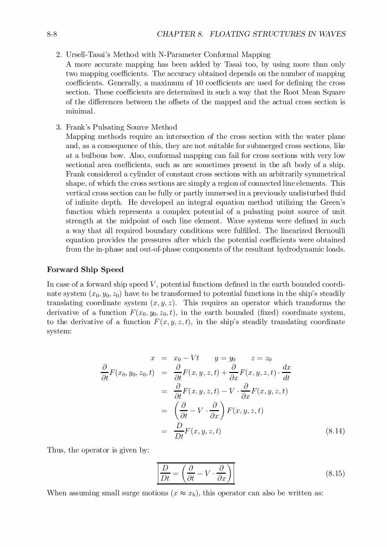
8-8 CHAPTER 8. FLOATING STRUCTURES IN WAVES
2. Ursell-Tasai’s Method with N-Parameter Conformal MappingA more accurate mapping has been added by Tasai too, by using more than onlytwo mapping coe¢cients. The accuracy obtained depends on the number of mappingcoe¢cients. Generally, a maximum of 10 coe¢cients are used for de…ning the crosssection. These coe¢cients are determined in such a way that the Root Mean Squareof the di¤erences between the o¤sets of the mapped and the actual cross section isminimal.
3. Frank’s Pulsating Source MethodMapping methods require an intersection of the cross section with the water planeand, as a consequence of this, they are not suitable for submerged cross sections, likeat a bulbous bow. Also, conformal mapping can fail for cross sections with very lowsectional area coe¢cients, such as are sometimes present in the aft body of a ship.Frank considered a cylinder of constant cross sections with an arbitrarily symmetricalshape, of which the cross sections are simply a region of connected line elements. Thisvertical cross section can be fully or partly immersed in a previously undisturbed ‡uidof in…nite depth. He developed an integral equation method utilizing the Green’sfunction which represents a complex potential of a pulsating point source of unitstrength at the midpoint of each line element. Wave systems were de…ned in sucha way that all required boundary conditions were ful…lled. The linearized Bernoulliequation provides the pressures after which the potential coe¢cients were obtainedfrom the in-phase and out-of-phase components of the resultant hydrodynamic loads.
Forward Ship Speed
In case of a forward ship speed V , potential functions de…ned in the earth bounded coordi-nate system (x0; y0; z0) have to be transformed to potential functions in the ship’s steadilytranslating coordinate system (x; y; z). This requires an operator which transforms thederivative of a function F (x0; y0; z0; t), in the earth bounded (…xed) coordinate system,to the derivative of a function F (x; y; z; t), in the ship’s steadily translating coordinatesystem:
x = x0 ¡ V t y = y0 z = z0@
@tF (x0; y0; z0; t) =
@
@tF (x; y; z; t) +
@
@xF (x; y; z; t) ¢ dx
dt
=@
@tF (x; y; z; t) ¡ V ¢ @
@xF (x; y; z; t)
=
µ@
@t¡ V ¢ @
@x
¶F (x; y; z; t)
=D
DtF (x; y; z; t) (8.14)
Thus, the operator is given by:
¯¯ DDt
=
µ@
@t¡ V ¢ @
@x
¶¯¯ (8.15)
When assuming small surge motions (x t xb), this operator can also be written as:
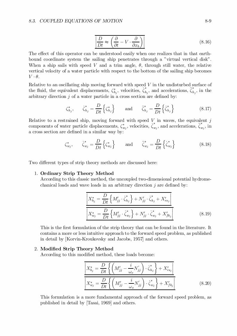
8.3. COUPLED EQUATIONS OF MOTION 8-9
¯¯ DDt
tµ@
@t¡ V ¢ @
@xb
¶¯¯ (8.16)
The e¤ect of this operator can be understood easily when one realizes that in that earth-bound coordinate system the sailing ship penetrates through a ”virtual vertical disk”.When a ship sails with speed V and a trim angle, µ, through still water, the relativevertical velocity of a water particle with respect to the bottom of the sailing ship becomesV ¢ µ.Relative to an oscillating ship moving forward with speed V in the undisturbed surface ofthe ‡uid, the equivalent displacements, ³¤hj , velocities, _³
¤hj
, and accelerations, ij¤hj
, in thearbitrary direction j of a water particle in a cross section are de…ned by:
³¤hj ,_³¤hj=D
Dt
n³¤hj
oand ij
¤hj=D
Dt
n_³¤hj
o(8.17)
Relative to a restrained ship, moving forward with speed V in waves, the equivalent jcomponents of water particle displacements, ³¤wj , velocities, _³
¤wj , and accelerations, ij
¤wj , in
a cross section are de…ned in a similar way by:
³¤wj ,_³¤wj =
D
Dt
n³¤wj
oand ij
¤wj =
D
Dt
n_³¤wj
o(8.18)
Two di¤erent types of strip theory methods are discussed here:
1. Ordinary Strip Theory MethodAccording to this classic method, the uncoupled two-dimensional potential hydrome-chanical loads and wave loads in an arbitrary direction j are de…ned by:
¯¯X¤
hj=D
Dt
nM0jj ¢ _³¤hj
o+N 0
jj ¢ _³¤hj +X 0rsj
¯¯
¯¯X¤
wj =D
Dt
nM 0jj ¢ _³¤wj
o+ N 0
jj ¢ _³¤wj +X 0fkj
¯¯ (8.19)
This is the …rst formulation of the strip theory that can be found in the literature. Itcontains a more or less intuitive approach to the forward speed problem, as publishedin detail by [Korvin-Kroukovsky and Jacobs, 1957] and others.
2. Modi…ed Strip Theory MethodAccording to this modi…ed method, these loads become:
¯¯X¤
hj=D
Dt
½µM 0jj ¡ i
!eN
0jj
¶¢ _³¤hj
¾+X 0
rsj
¯¯
¯¯X¤
wj =D
Dt
½µM 0jj ¡ i
!eN
0jj
¶¢ _³¤wj
¾+X 0
fkj
¯¯ (8.20)
This formulation is a more fundamental approach of the forward speed problem, aspublished in detail by [Tasai, 1969] and others.
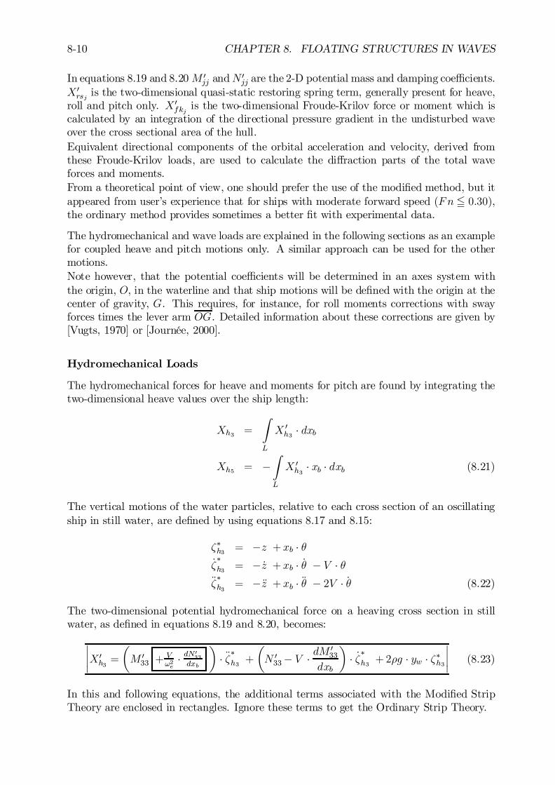
8-10 CHAPTER 8. FLOATING STRUCTURES IN WAVES
In equations 8.19 and 8.20M 0jj andN 0
jj are the 2-D potential mass and damping coe¢cients.X 0rsj is the two-dimensional quasi-static restoring spring term, generally present for heave,
roll and pitch only. X 0fkj
is the two-dimensional Froude-Krilov force or moment which iscalculated by an integration of the directional pressure gradient in the undisturbed waveover the cross sectional area of the hull.Equivalent directional components of the orbital acceleration and velocity, derived fromthese Froude-Krilov loads, are used to calculate the di¤raction parts of the total waveforces and moments.From a theoretical point of view, one should prefer the use of the modi…ed method, but itappeared from user’s experience that for ships with moderate forward speed (Fn5 0:30),the ordinary method provides sometimes a better …t with experimental data.
The hydromechanical and wave loads are explained in the following sections as an examplefor coupled heave and pitch motions only. A similar approach can be used for the othermotions.Note however, that the potential coe¢cients will be determined in an axes system withthe origin, O, in the waterline and that ship motions will be de…ned with the origin at thecenter of gravity, G. This requires, for instance, for roll moments corrections with swayforces times the lever arm OG. Detailed information about these corrections are given by[Vugts, 1970] or [Journée, 2000].
Hydromechanical Loads
The hydromechanical forces for heave and moments for pitch are found by integrating thetwo-dimensional heave values over the ship length:
Xh3 =
Z
L
X 0h3 ¢ dxb
Xh5 = ¡Z
L
X 0h3
¢ xb ¢ dxb (8.21)
The vertical motions of the water particles, relative to each cross section of an oscillatingship in still water, are de…ned by using equations 8.17 and 8.15:
³¤h3 = ¡z + xb ¢ µ_³¤h3 = ¡ _z + xb ¢ _µ ¡ V ¢ µÄ³¤h3
= ¡Äz + xb ¢ ĵ ¡ 2V ¢ _µ (8.22)
The two-dimensional potential hydromechanical force on a heaving cross section in stillwater, as de…ned in equations 8.19 and 8.20, becomes:
¯¯X 0
h3=
µM 033 +
V!2e
¢ dN033
dxb
¶¢ ij¤h3 +
µN 033¡ V ¢ dM
033
dxb
¶¢ _³¤h3 +2½g ¢ yw ¢ ³¤h3
¯¯ (8.23)
In this and following equations, the additional terms associated with the Modi…ed StripTheory are enclosed in rectangles. Ignore these terms to get the Ordinary Strip Theory.
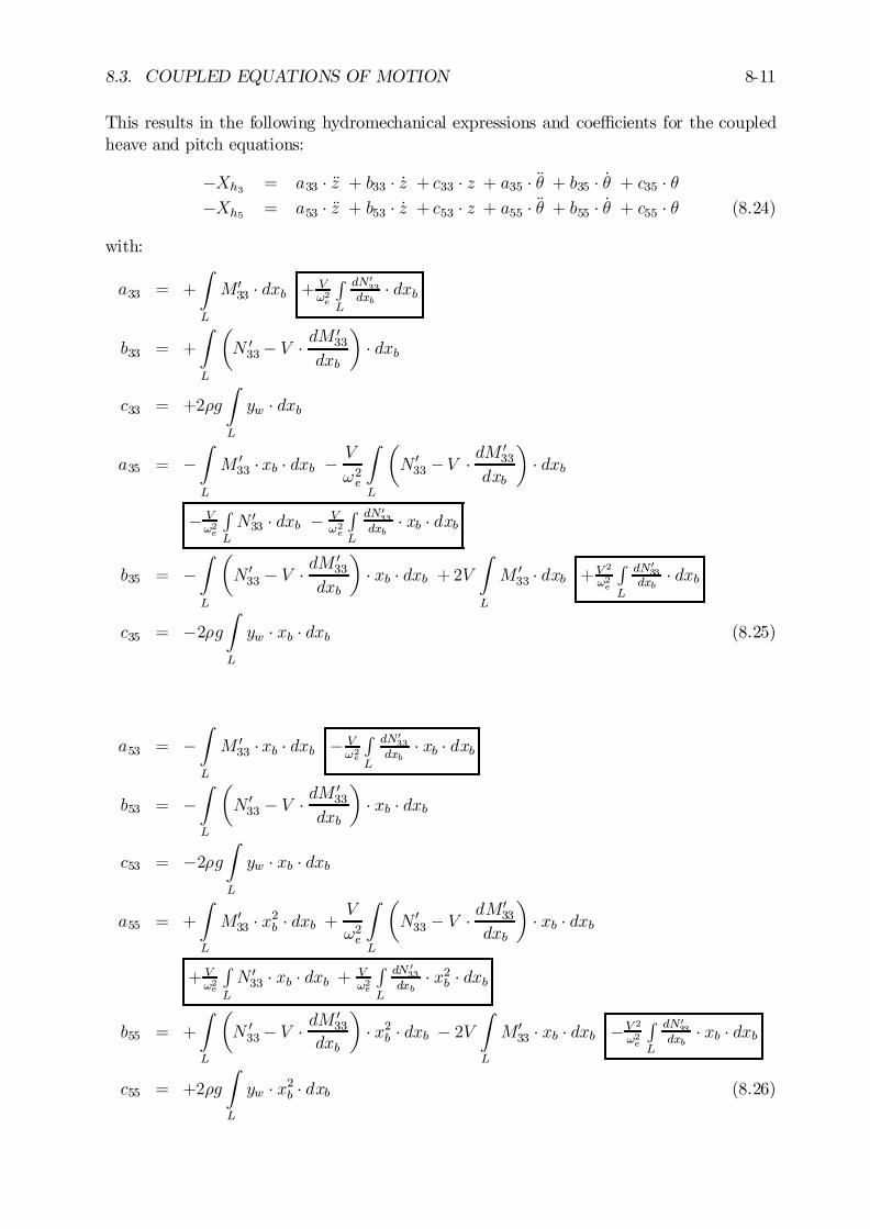
8.3. COUPLED EQUATIONS OF MOTION 8-11
This results in the following hydromechanical expressions and coe¢cients for the coupledheave and pitch equations:
¡Xh3 = a33 ¢ Äz + b33 ¢ _z + c33 ¢ z + a35 ¢ ĵ + b35 ¢ _µ + c35 ¢ µ¡Xh5 = a53 ¢ Äz + b53 ¢ _z + c53 ¢ z + a55 ¢ ĵ + b55 ¢ _µ + c55 ¢ µ (8.24)
with:
a33 = +
Z
L
M033 ¢ dxb + V
!2e
RL
dN033
dxb¢ dxb
b33 = +
Z
L
µN 033¡ V ¢ dM
033
dxb
¶¢ dxb
c33 = +2½g
Z
L
yw ¢ dxb
a35 = ¡Z
L
M 033 ¢xb ¢ dxb ¡ V
!2e
Z
L
µN 033 ¡V ¢ dM
033
dxb
¶¢ dxb
¡ V!2e
RL
N 033 ¢ dxb ¡ V
!2e
RL
dN033
dxb¢ xb ¢ dxb
b35 = ¡Z
L
µN 033 ¡ V ¢ dM
033
dxb
¶¢ xb ¢ dxb +2V
Z
L
M 033 ¢ dxb +V 2
!2e
RL
dN033
dxb¢ dxb
c35 = ¡2½gZ
L
yw ¢ xb ¢ dxb (8.25)
a53 = ¡Z
L
M 033 ¢xb ¢ dxb ¡ V
!2e
RL
dN033
dxb¢ xb ¢ dxb
b53 = ¡Z
L
µN 033 ¡ V ¢ dM
033
dxb
¶¢ xb ¢ dxb
c53 = ¡2½gZ
L
yw ¢ xb ¢ dxb
a55 = +
Z
L
M033 ¢ x2b ¢ dxb +
V
!2e
Z
L
µN 033 ¡ V ¢ dM
033
dxb
¶¢ xb ¢ dxb
+ V!2e
RL
N 033 ¢ xb ¢ dxb + V
!2e
RL
dN 033
dxb¢ x2b ¢ dxb
b55 = +
Z
L
µN 033¡ V ¢ dM
033
dxb
¶¢ x2b ¢ dxb ¡ 2V
Z
L
M033 ¢ xb ¢ dxb ¡V 2
!2e
RL
dN033
dxb¢ xb ¢ dxb
c55 = +2½g
Z
L
yw ¢ x2b ¢ dxb (8.26)
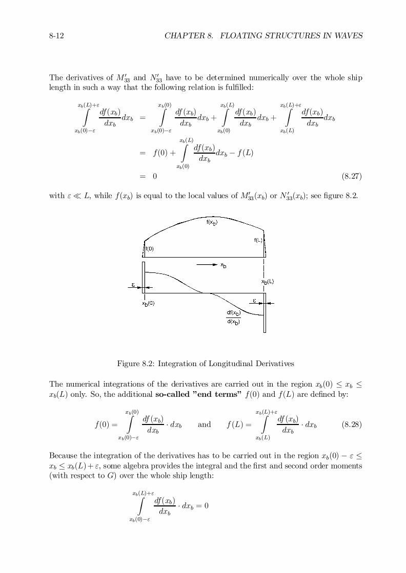
8-12 CHAPTER 8. FLOATING STRUCTURES IN WAVES
The derivatives of M 033 and N 0
33 have to be determined numerically over the whole shiplength in such a way that the following relation is ful…lled:
xb(L)+"Z
xb(0)¡"
df(xb)
dxbdxb =
xb(0)Z
xb(0)¡"
df (xb)
dxbdxb +
xb(L)Z
xb(0)
df(xb)
dxbdxb +
xb(L)+"Z
xb(L)
df(xb)
dxbdxb
= f(0) +
xb(L)Z
xb(0)
df(xb)
dxbdxb ¡ f (L)
= 0 (8.27)
with "¿ L, while f(xb) is equal to the local values of M033(xb) or N 0
33(xb); see …gure 8.2.
Figure 8.2: Integration of Longitudinal Derivatives
The numerical integrations of the derivatives are carried out in the region xb(0) · xb ·xb(L) only. So, the additional so-called ”end terms” f(0) and f(L) are de…ned by:
f(0) =
xb(0)Z
xb(0)¡"
df (xb)
dxb¢ dxb and f (L) =
xb(L)+"Z
xb(L)
df (xb)
dxb¢ dxb (8.28)
Because the integration of the derivatives has to be carried out in the region xb(0) ¡ " ·xb · xb(L)+ ", some algebra provides the integral and the …rst and second order moments(with respect to G) over the whole ship length:
xb(L)+"Z
xb(0)¡"
df(xb)
dxb¢ dxb = 0
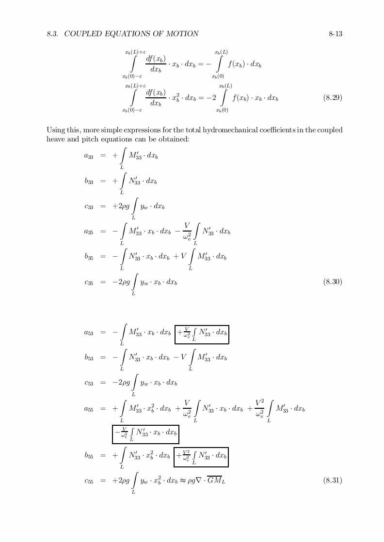
8.3. COUPLED EQUATIONS OF MOTION 8-13
xb(L)+"Z
xb(0)¡"
df(xb)
dxb¢ xb ¢ dxb = ¡
xb(L)Z
xb(0)
f(xb) ¢ dxb
xb(L)+"Z
xb(0)¡"
df(xb)
dxb¢ x2b ¢ dxb = ¡2
xb(L)Z
xb(0)
f(xb) ¢ xb ¢ dxb (8.29)
Using this, more simple expressions for the total hydromechanical coe¢cients in the coupledheave and pitch equations can be obtained:
a33 = +
Z
L
M 033 ¢ dxb
b33 = +
Z
L
N 033 ¢ dxb
c33 = +2½g
Z
L
yw ¢ dxb
a35 = ¡Z
L
M 033 ¢ xb ¢ dxb ¡ V
!2e
Z
L
N 033 ¢ dxb
b35 = ¡Z
L
N 033 ¢ xb ¢ dxb + V
Z
L
M 033 ¢ dxb
c35 = ¡2½gZ
L
yw ¢ xb ¢ dxb (8.30)
a53 = ¡Z
L
M 033 ¢ xb ¢ dxb + V
!2e
RL
N 033 ¢ dxb
b53 = ¡Z
L
N 033 ¢ xb ¢ dxb ¡ V
Z
L
M 033 ¢ dxb
c53 = ¡2½gZ
L
yw ¢ xb ¢ dxb
a55 = +
Z
L
M 033 ¢ x2b ¢ dxb +
V
!2e
Z
L
N 033 ¢ xb ¢ dxb +
V 2
!2e
Z
L
M033 ¢ dxb
¡ V!2e
RL
N 033 ¢ xb ¢ dxb
b55 = +
Z
L
N 033 ¢ x2b ¢ dxb +V 2
!2e
RL
N 033 ¢ dxb
c55 = +2½g
Z
L
yw ¢ x2b ¢ dxb t ½gr ¢GML (8.31)
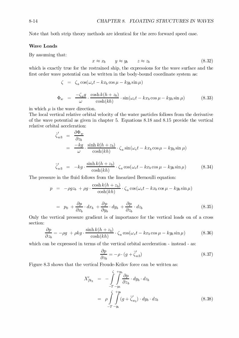
8-14 CHAPTER 8. FLOATING STRUCTURES IN WAVES
Note that both strip theory methods are identical for the zero forward speed case.
Wave Loads
By assuming that:x ¼ xb y ¼ yb z ¼ zb (8.32)
which is exactly true for the restrained ship, the expressions for the wave surface and the…rst order wave potential can be written in the body-bound coordinate system as:
³ = ³a cos(!et¡ kxb cos¹¡ kyb sin¹)
©w =¡³ag!
¢ coshk(h+ zb)cosh(kh)
¢ sin(!et¡ kxb cos¹¡ kyb sin ¹) (8.33)
in which ¹ is the wave direction.The local vertical relative orbital velocity of the water particles follows from the derivativeof the wave potential as given in chapter 5. Equations 8.18 and 8.15 provide the verticalrelative orbital acceleration:
_³0w3 =
@©w@zb
=¡kg!
¢ sinh k(h + zb)cosh(kh)
¢ ³a sin(!et¡ kxb cos¹¡ kyb sin ¹)
ij0w3 = ¡kg ¢ sinhk(h + zb)
cosh(kh)¢ ³a cos(!et¡ kxb cos¹¡ kyb sin¹) (8.34)
The pressure in the ‡uid follows from the linearized Bernoulli equation:
p = ¡½gzb + ½g ¢ coshk(h + zb)cosh(kh)
¢ ³a cos(!et¡ kxb cos¹¡ kyb sin¹)
= p0 +@p
@xb¢ dxb +
@p
@yb¢ dyb +
@p
@zb¢ dzb (8.35)
Only the vertical pressure gradient is of importance for the vertical loads on of a crosssection:
@p
@zb= ¡½g + ½kg ¢ sinhk(h + zb)
cosh(kh)¢ ³a cos(!et¡ kxb cos¹¡ kyb sin¹) (8.36)
which can be expressed in terms of the vertical orbital acceleration - instead - as:
@p
@zb= ¡½ ¢ (g + ij 0w3) (8.37)
Figure 8.3 shows that the vertical Froude-Krilov force can be written as:
X 0fk3
= ¡³Z
¡T
+ybZ
¡yb
@p
@zb¢ dyb ¢ dzb
= ½
³Z
¡T
+ybZ
¡yb
(g+ ij0w3) ¢ dyb ¢ dzb (8.38)
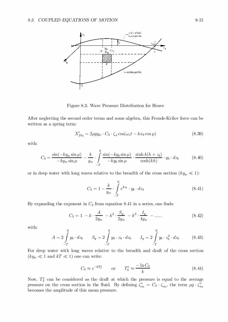
8.3. COUPLED EQUATIONS OF MOTION 8-15
Figure 8.3: Wave Pressure Distribution for Heave
After neglecting the second order terms and some algebra, this Froude-Krilov force can bewritten as a spring term:
X 0fk3 = 2½gyw ¢ C3 ¢ ³a cos(!et ¡ kxb cos¹) (8.39)
with:
C3 =sin(¡kyw sin¹)
¡kyw sin¹¡ k
yw¢
0Z
¡T
sin(¡kyb sin¹)¡kyb sin¹
¢ sinh k(h + zb)cosh(kh)
¢ yb ¢ dzb (8.40)
or in deep water with long waves relative to the breadth of the cross section (kyw ¿ 1):
C3 = 1¡ k
yw¢
0Z
¡T
ekzb ¢ yb ¢ dzb (8.41)
By expanding the exponent in C3 from equation 8.41 in a series, one …nds:
C3 = 1 ¡ k ¢ A2yw
¡ k2 ¢ Sy2yw
¡ k3 ¢ Iy4yw
¡ :::::: (8.42)
with:
A = 2
0Z
¡T
yb ¢ dzb Sy = 2
0Z
¡T
yb ¢ zb ¢ dzb Iy = 2
0Z
¡T
yb ¢ z2b ¢ dzb (8.43)
For deep water with long waves relative to the breadth and draft of the cross section(kyw ¿ 1 and kT ¿ 1) one can write:
C3 ¼ e¡kT¤3 or T ¤3 ¼ ¡ lnC3
k(8.44)
Now, T ¤3 can be considered as the draft at which the pressure is equal to the averagepressure on the cross section in the ‡uid. By de…ning ³¤a3 = C3 ¢ ³a3, the term ½g ¢ ³¤a3becomes the amplitude of this mean pressure.
8-16 CHAPTER 8. FLOATING STRUCTURES IN WAVES
The e¤ective vertical components of the orbital accelerations and velocities in undisturbedwaves are de…ned at this draft T ¤3 too:
ij¤w3
= ¡kg ¢ ³¤a3 cos(!et¡ kxb cos¹)
_³¤w3
=¡kg!
¢ ³¤a3 sin(!et¡ kxb cos¹) (8.45)
With this, the two-dimensional wave exciting force on a restrained cross section of a shipin waves, as de…ned in equations 8.19 and 8.20, becomes:
X 0w3 =
µM033 +
V!2e
¢ dN033
dxb
¶¢ ij¤w3 +
µN 033 ¡ V ¢ dM
033
dxb
¶¢ _³¤w3 +X 0
fk3 (8.46)
in which only the modi…ed strip theory includes the outlined term.These equivalent accelerations and velocities in the undisturbed wave are used todetermine the additional wave loads due to di¤raction of the waves. They are consideredas potential mass and damping terms, just as applied for the hydromechanical loads. Thisis the reason why this approach called the relative motion principle in strip theory.The total wave loads for heave and pitch follows from all this:
Xw3 = +
Z
L
M 033 ¢ ij ¤w3 ¢ dxb + V
!¢!eRL
dN033
dxb¢ ij¤w3 ¢ dxb
+
Z
L
µ!!e
¢ N 033 ¡ V ¢ dM
033
dxb
¶¢ _³¤w3 ¢ dxb
+
Z
L
X 0fk3 ¢ dxb (8.47)
Xw5 = ¡Z
L
M 033 ¢ xb ¢ ij¤w3 ¢ dxb ¡ V
!¢!eRL
dN033
dxb¢ xb ¢ ij¤w3 ¢ dxb
¡Z
L
µ!!e
¢ N 033 ¡ V ¢ dM
033
dxb
¶¢ xb ¢ _³¤w3 ¢ dxb
¡Z
L
X 0fk3 ¢ xb ¢ dxb (8.48)
Note that both strip theory methods are identical here for the zero forward speed case andthat the (generally small) in‡uence of the surge wave loads on the pitch wave moment hasbeen ignored here, too.
Heave and Pitch Equations
Putting all this together yields the coupled equations of motion of heave and pitch:
(½r + a33) ¢ Äz + b33 ¢ _z + c33 ¢ z + a35 ¢ ĵ + b35 ¢ _µ + c35 ¢ µ = Xw3a53 ¢ Äz + b53 ¢ _z + c53 ¢ z + (Ixx+ a55) ¢ ĵ + b55 ¢ _µ + c55 ¢ µ = Xw5 (8.49)
which can be solved as described in chapter 6.
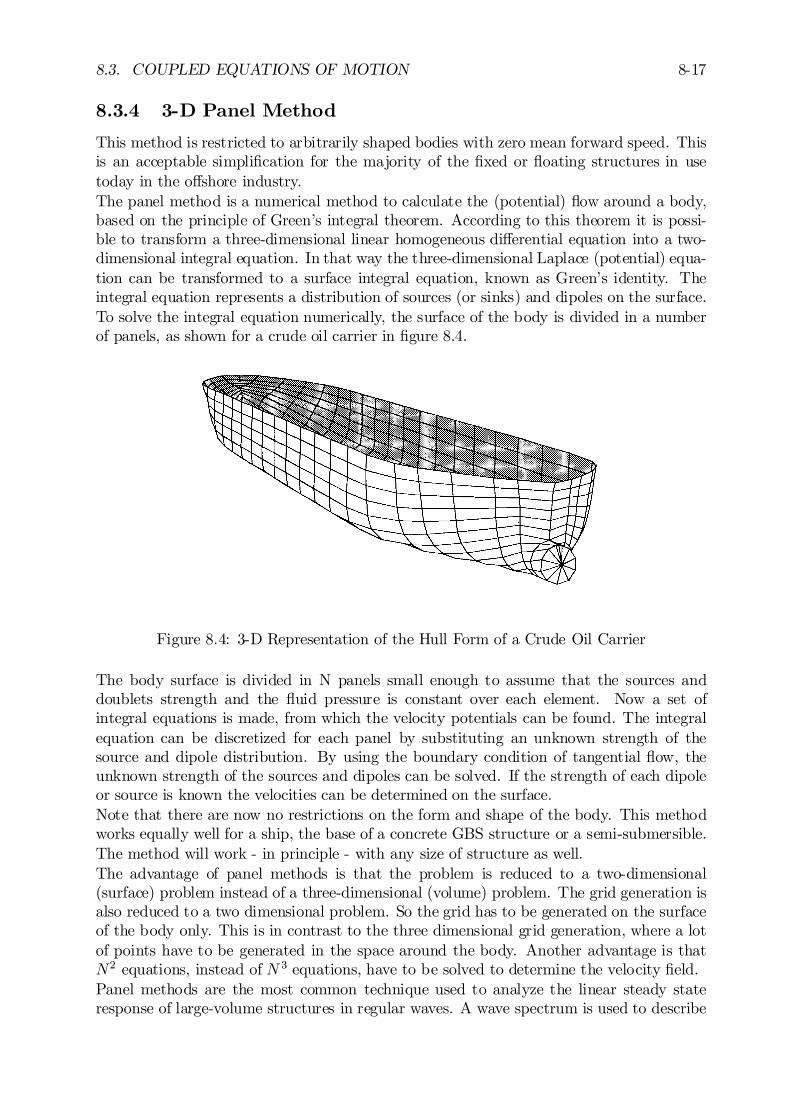
8.3. COUPLED EQUATIONS OF MOTION 8-17
8.3.4 3-D Panel Method
This method is restricted to arbitrarily shaped bodies with zero mean forward speed. Thisis an acceptable simpli…cation for the majority of the …xed or ‡oating structures in usetoday in the o¤shore industry.The panel method is a numerical method to calculate the (potential) ‡ow around a body,based on the principle of Green’s integral theorem. According to this theorem it is possi-ble to transform a three-dimensional linear homogeneous di¤erential equation into a two-dimensional integral equation. In that way the three-dimensional Laplace (potential) equa-tion can be transformed to a surface integral equation, known as Green’s identity. Theintegral equation represents a distribution of sources (or sinks) and dipoles on the surface.To solve the integral equation numerically, the surface of the body is divided in a numberof panels, as shown for a crude oil carrier in …gure 8.4.
Figure 8.4: 3-D Representation of the Hull Form of a Crude Oil Carrier
The body surface is divided in N panels small enough to assume that the sources anddoublets strength and the ‡uid pressure is constant over each element. Now a set ofintegral equations is made, from which the velocity potentials can be found. The integralequation can be discretized for each panel by substituting an unknown strength of thesource and dipole distribution. By using the boundary condition of tangential ‡ow, theunknown strength of the sources and dipoles can be solved. If the strength of each dipoleor source is known the velocities can be determined on the surface.Note that there are now no restrictions on the form and shape of the body. This methodworks equally well for a ship, the base of a concrete GBS structure or a semi-submersible.The method will work - in principle - with any size of structure as well.The advantage of panel methods is that the problem is reduced to a two-dimensional(surface) problem instead of a three-dimensional (volume) problem. The grid generation isalso reduced to a two dimensional problem. So the grid has to be generated on the surfaceof the body only. This is in contrast to the three dimensional grid generation, where a lotof points have to be generated in the space around the body. Another advantage is thatN2 equations, instead of N 3 equations, have to be solved to determine the velocity …eld.Panel methods are the most common technique used to analyze the linear steady stateresponse of large-volume structures in regular waves. A wave spectrum is used to describe
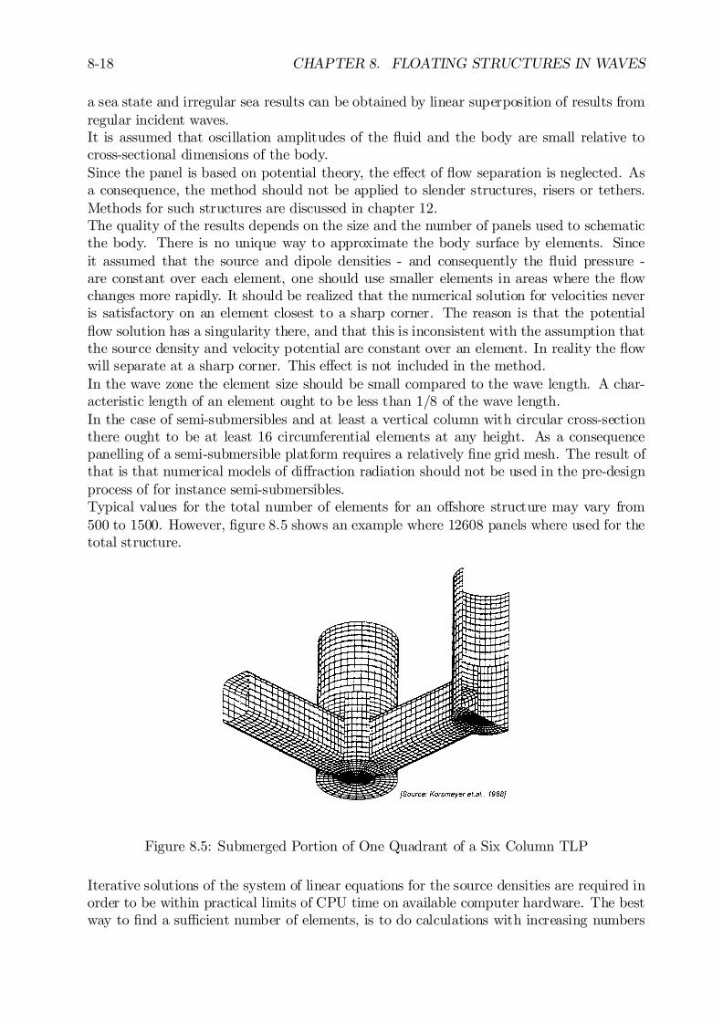
8-18 CHAPTER 8. FLOATING STRUCTURES IN WAVES
a sea state and irregular sea results can be obtained by linear superposition of results fromregular incident waves.It is assumed that oscillation amplitudes of the ‡uid and the body are small relative tocross-sectional dimensions of the body.Since the panel is based on potential theory, the e¤ect of ‡ow separation is neglected. Asa consequence, the method should not be applied to slender structures, risers or tethers.Methods for such structures are discussed in chapter 12.The quality of the results depends on the size and the number of panels used to schematicthe body. There is no unique way to approximate the body surface by elements. Sinceit assumed that the source and dipole densities - and consequently the ‡uid pressure -are constant over each element, one should use smaller elements in areas where the ‡owchanges more rapidly. It should be realized that the numerical solution for velocities neveris satisfactory on an element closest to a sharp corner. The reason is that the potential‡ow solution has a singularity there, and that this is inconsistent with the assumption thatthe source density and velocity potential are constant over an element. In reality the ‡owwill separate at a sharp corner. This e¤ect is not included in the method.In the wave zone the element size should be small compared to the wave length. A char-acteristic length of an element ought to be less than 1/8 of the wave length.In the case of semi-submersibles and at least a vertical column with circular cross-sectionthere ought to be at least 16 circumferential elements at any height. As a consequencepanelling of a semi-submersible platform requires a relatively …ne grid mesh. The result ofthat is that numerical models of di¤raction radiation should not be used in the pre-designprocess of for instance semi-submersibles.Typical values for the total number of elements for an o¤shore structure may vary from500 to 1500. However, …gure 8.5 shows an example where 12608 panels where used for thetotal structure.
Figure 8.5: Submerged Portion of One Quadrant of a Six Column TLP
Iterative solutions of the system of linear equations for the source densities are required inorder to be within practical limits of CPU time on available computer hardware. The bestway to …nd a su¢cient number of elements, is to do calculations with increasing numbers
8.4. MOTIONS IN REGULAR WAVES 8-19
of elements and check the convergence of the results.Methods to evaluate the hydrodynamic loads and motions of ‡oating or …xed structuresin waves have been developed based on linear three-dimensional potential theory, see forinstance [Oortmerssen, 1976a]. Both, the wave-frequency hydrodynamic loads on free-‡oating or …xed bodies and the wave-frequency motions of ‡oating bodies as well as thesecond order wave drift forces can be computed. Experimental veri…cation of results ofcomputations has been carried out for bodies with a large variety of shapes. Such com-parisons have shown that 3-D di¤raction methods generally can be applied to most bodyshapes and are therefore a good tool to investigate such e¤ects.It may be noted that the 3-D method as described here is suitable for the zero forwardspeed case only. Generally the potential coe¢cients are determined in a coordinate systemwith G= O in the water line, so that a correction for the actual OG-value is required.
8.4 Motions in Regular Waves
Each equation of motion can be split into an equation with in-phase parts and an equationwith out-of-phase components. After dividing the left and right hand terms of these equa-tions by the wave amplitude ³a, two sets of six coupled equations of motion are available.The unknown variables in the 6 coupled equations of motions in the vertical plane are:
surge: xa³a
¢ cos "x³ and xa³a
¢ sin "x³
heave: za³a
¢ cos "z³ and za³a
¢ sin "z³
pitch: µa³a
¢ cos "µ³ and µa³a
¢ sin "µ³
9>>>>>=>>>>>;
(8.50)
The unknown variables in the 6 coupled equations of motions in the horizontal planeare:
sway: ya³a
¢ cos "y³ and ya³a
¢ sin "y³
roll: Áa³a
¢ cos "Á³ and Áa³a
¢ sin "Á³
yaw: Ãa³a
¢ cos "ó and Ãa³a
¢ sin "ó
9>>>>>=>>>>>;
(8.51)
These 2 sets of equations of motion have to be solved numerically. Their terms are explainedbelow.
8.4.1 Frequency Characteristics
The transfer functions (also called response amplitude operators) of the motions arethe motion amplitude component to wave amplitude ratios. They and the phase shifts ofthese motions relative to the (virtual) wave elevation at the ship’s center of gravity followfrom the solution to 8.50 and 8.51:
xa³a
ya³a
za³a
µa³a
Áa³a
Ãa³a
and
"x³ "y³ "z³ "µ³ "Á³ "ó
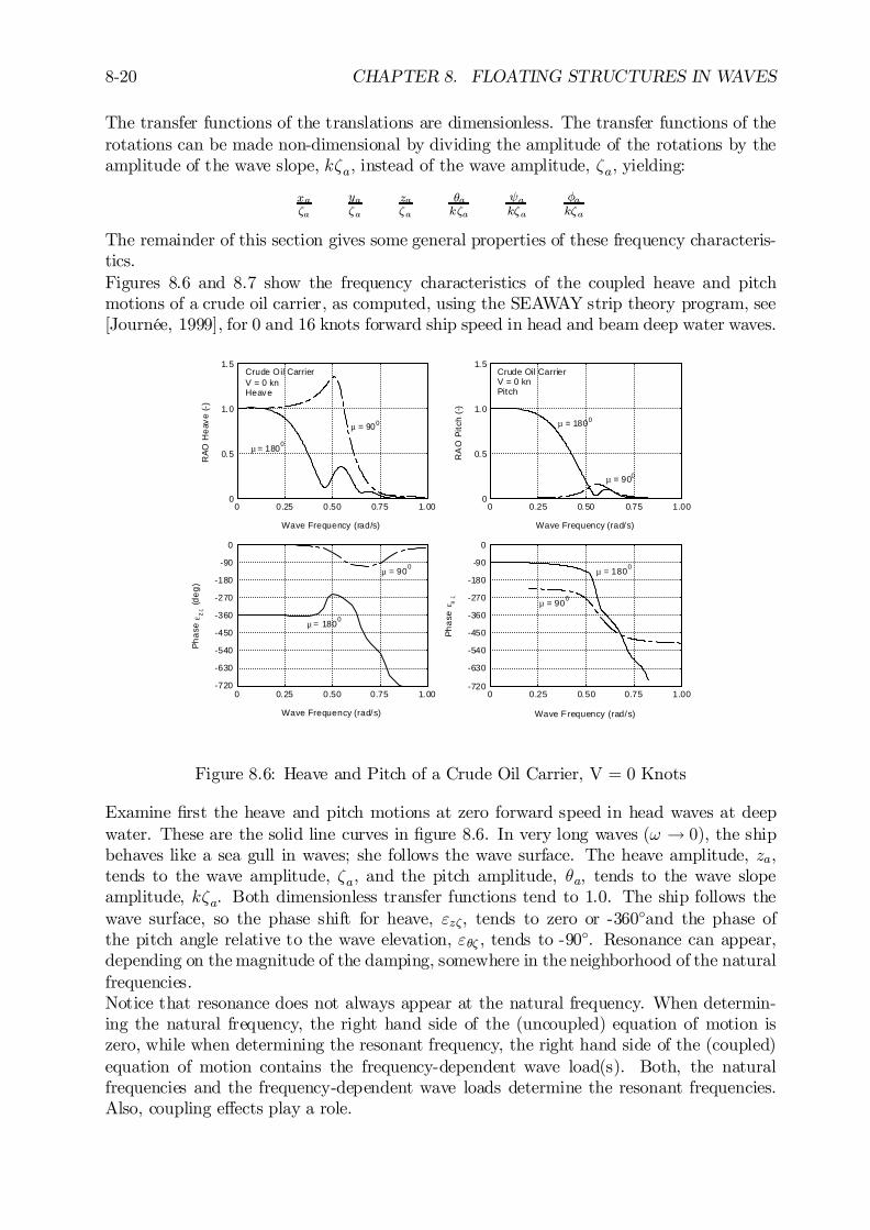
8-20 CHAPTER 8. FLOATING STRUCTURES IN WAVES
The transfer functions of the translations are dimensionless. The transfer functions of therotations can be made non-dimensional by dividing the amplitude of the rotations by theamplitude of the wave slope, k³a, instead of the wave amplitude, ³a, yielding:
xa³a
ya³a
za³a
µak³a
Ãak³a
Áak³a
The remainder of this section gives some general properties of these frequency characteris-tics.Figures 8.6 and 8.7 show the frequency characteristics of the coupled heave and pitchmotions of a crude oil carrier, as computed, using the SEAWAY strip theory program, see[Journée, 1999], for 0 and 16 knots forward ship speed in head and beam deep water waves.
-720
-630
-540
-450
-360
-270
-180
-90
0
0 0.25 0.50 0.75 1.00
µ = 900
µ = 1800
Wave Frequency (rad/s)
Phas
e ε z
ζ (deg
)
0
0.5
1.0
1.5
0 0.25 0.50 0.75 1.00
Crude Oil CarrierV = 0 knHeave
µ = 900
µ = 1800
Wave Frequency (rad/s)
RAO
Hea
ve (-
)
0
0.5
1.0
1.5
0 0.25 0.50 0.75 1.00
Crude Oil CarrierV = 0 knPitch
µ = 900
µ = 1800
Wave Frequency (rad/s)
RA
O P
itch
(-)
-720
-630
-540
-450
-360
-270
-180
-90
0
0 0.25 0.50 0.75 1.00
µ = 900
µ = 1800
Wave F requency (rad/s)
Phas
e ε θ
ζ
Figure 8.6: Heave and Pitch of a Crude Oil Carrier, V = 0 Knots
Examine …rst the heave and pitch motions at zero forward speed in head waves at deepwater. These are the solid line curves in …gure 8.6. In very long waves (! ! 0), the shipbehaves like a sea gull in waves; she follows the wave surface. The heave amplitude, za,tends to the wave amplitude, ³a, and the pitch amplitude, µa, tends to the wave slopeamplitude, k³a. Both dimensionless transfer functions tend to 1.0. The ship follows thewave surface, so the phase shift for heave, "z³, tends to zero or -360±and the phase ofthe pitch angle relative to the wave elevation, "µ³ , tends to -90±. Resonance can appear,depending on the magnitude of the damping, somewhere in the neighborhood of the naturalfrequencies.Notice that resonance does not always appear at the natural frequency. When determin-ing the natural frequency, the right hand side of the (uncoupled) equation of motion iszero, while when determining the resonant frequency, the right hand side of the (coupled)equation of motion contains the frequency-dependent wave load(s). Both, the naturalfrequencies and the frequency-dependent wave loads determine the resonant frequencies.Also, coupling e¤ects play a role.
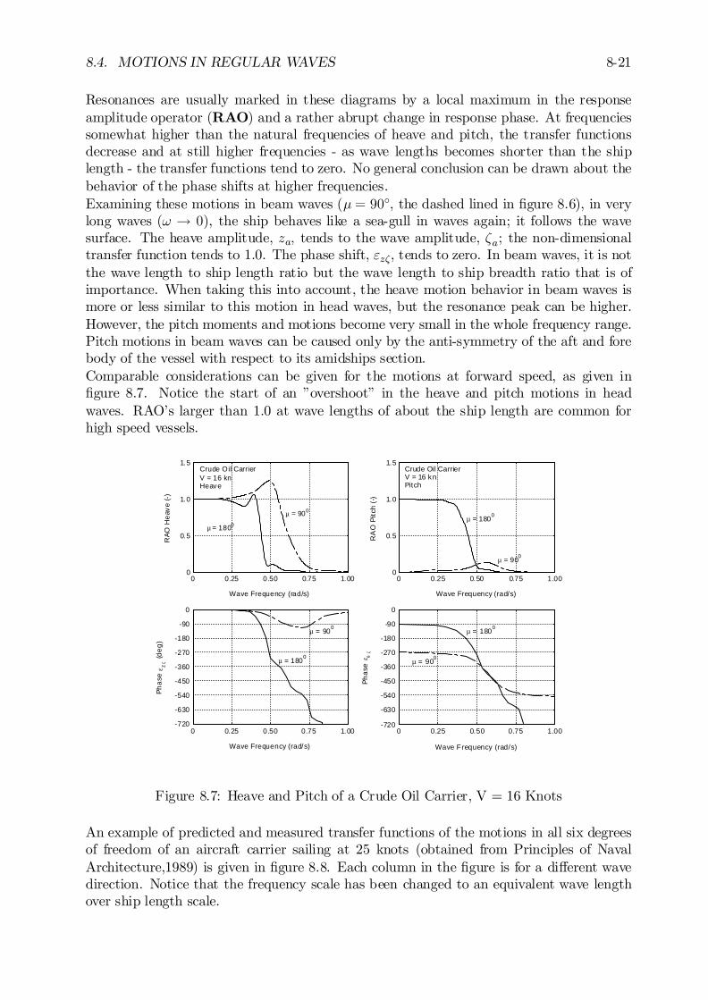
8.4. MOTIONS IN REGULAR WAVES 8-21
Resonances are usually marked in these diagrams by a local maximum in the responseamplitude operator (RAO) and a rather abrupt change in response phase. At frequenciessomewhat higher than the natural frequencies of heave and pitch, the transfer functionsdecrease and at still higher frequencies - as wave lengths becomes shorter than the shiplength - the transfer functions tend to zero. No general conclusion can be drawn about thebehavior of the phase shifts at higher frequencies.Examining these motions in beam waves (¹= 90±, the dashed lined in …gure 8.6), in verylong waves (! ! 0), the ship behaves like a sea-gull in waves again; it follows the wavesurface. The heave amplitude, za; tends to the wave amplitude, ³a; the non-dimensionaltransfer function tends to 1.0. The phase shift, "z³, tends to zero. In beam waves, it is notthe wave length to ship length ratio but the wave length to ship breadth ratio that is ofimportance. When taking this into account, the heave motion behavior in beam waves ismore or less similar to this motion in head waves, but the resonance peak can be higher.However, the pitch moments and motions become very small in the whole frequency range.Pitch motions in beam waves can be caused only by the anti-symmetry of the aft and forebody of the vessel with respect to its amidships section.Comparable considerations can be given for the motions at forward speed, as given in…gure 8.7. Notice the start of an ”overshoot” in the heave and pitch motions in headwaves. RAO’s larger than 1.0 at wave lengths of about the ship length are common forhigh speed vessels.
0
0.5
1.0
1.5
0 0.25 0.50 0.75 1.00
Crude Oil CarrierV = 16 knHeave
µ = 900
µ = 1800
Wave Frequency (rad/s)
RAO
Hea
ve (-
)
-720
-630
-540
-450
-360
-270
-180
-90
0
0 0.25 0.50 0.75 1.00
µ = 900
µ = 1800
Wave Frequency (rad/s)
Phas
e ε z
ζ (deg
)
0
0.5
1.0
1.5
0 0.25 0.50 0.75 1.00
Crude Oil CarrierV = 16 knPitch
µ = 900
µ = 1800
Wave Frequency (rad/s)
RA
O P
itch
(-)
-720
-630
-540
-450
-360
-270
-180
-90
0
0 0.25 0.50 0.75 1.00
µ = 900
µ = 1800
Wave F requency (rad/s)
Phas
e ε θ
ζ
Figure 8.7: Heave and Pitch of a Crude Oil Carrier, V = 16 Knots
An example of predicted and measured transfer functions of the motions in all six degreesof freedom of an aircraft carrier sailing at 25 knots (obtained from Principles of NavalArchitecture,1989) is given in …gure 8.8. Each column in the …gure is for a di¤erent wavedirection. Notice that the frequency scale has been changed to an equivalent wave lengthover ship length scale.
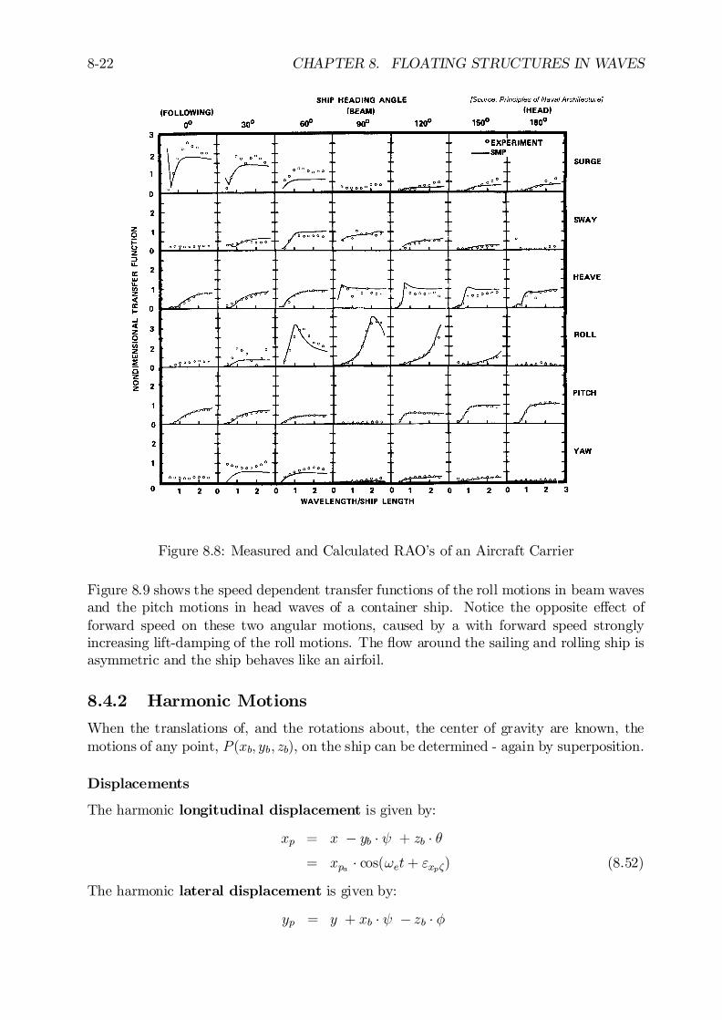
8-22 CHAPTER 8. FLOATING STRUCTURES IN WAVES
Figure 8.8: Measured and Calculated RAO’s of an Aircraft Carrier
Figure 8.9 shows the speed dependent transfer functions of the roll motions in beam wavesand the pitch motions in head waves of a container ship. Notice the opposite e¤ect offorward speed on these two angular motions, caused by a with forward speed stronglyincreasing lift-damping of the roll motions. The ‡ow around the sailing and rolling ship isasymmetric and the ship behaves like an airfoil.
8.4.2 Harmonic Motions
When the translations of, and the rotations about, the center of gravity are known, themotions of any point, P (xb; yb; zb), on the ship can be determined - again by superposition.
Displacements
The harmonic longitudinal displacement is given by:
xp = x ¡ yb ¢ Ã + zb ¢ µ= xpa ¢ cos(!et+ "xp³) (8.52)
The harmonic lateral displacement is given by:
yp = y + xb ¢ Ã ¡ zb ¢ Á
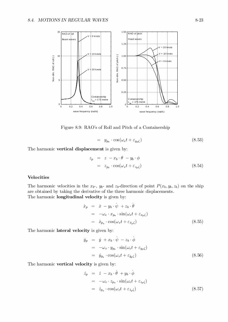
8.4. MOTIONS IN REGULAR WAVES 8-23
0
0.25
0.50
0.75
1.00
1.25
1.50
0 0.2 0.4 0.6 0.8 1.0
R AO of pitch H ead waves
C ontainershipL
pp = 175 metre
V = 0 knots
V = 10 knots
V = 20 knots
wave frequency (rad/s )
Non
-dim
. RA
O o
f pitc
h (-
)
0
5
10
15
0 0.2 0.4 0.6 0.8 1.0
RAO of roll Beam waves
ContainershipL
pp = 175 metre
V = 20 knots
V = 10 knots
V = 0 knots
wave frequency (rad/s)
Non
-dim
. RAO
of r
oll (
-)
Figure 8.9: RAO’s of Roll and Pitch of a Containership
= ypa ¢ cos(!et+ "yp³ ) (8.53)
The harmonic vertical displacement is given by:
zp = z ¡ xb ¢ µ ¡ yb ¢ Á= zpa ¢ cos(!et+ "zp³) (8.54)
Velocities
The harmonic velocities in the xb-, yb- and zb-direction of point P (xb; yb; zb) on the shipare obtained by taking the derivative of the three harmonic displacements.The harmonic longitudinal velocity is given by:
_xp = _x ¡ yb ¢ _Ã + zb ¢ _µ= ¡!e ¢ xpa ¢ sin(!et+ "xp³ )= _xpa ¢ cos(!et+ " _xp³) (8.55)
The harmonic lateral velocity is given by:
_yp = _y + xb ¢ _Ã ¡ zb ¢ _Á= ¡!e ¢ ypa ¢ sin(!et+ "yp³)= _ypa ¢ cos(!et+ " _yp³ ) (8.56)
The harmonic vertical velocity is given by:
_zp = _z ¡ xb ¢ _µ + yb ¢ _Á= ¡!e ¢ zpa ¢ sin(!et+ "zp³)= _zpa ¢ cos(!et + " _zp³) (8.57)

8-24 CHAPTER 8. FLOATING STRUCTURES IN WAVES
Accelerations
The harmonic accelerations in the xb-, yb- and zb-direction of point P (xb; yb; zb) on theship are obtained by taking the second derivative of the three harmonic displacements.However, in a ship-bound axes system, a longitudinal and transverse component of theacceleration of gravity, g, has to be added to the longitudinal and lateral accelerationsrespectively; this yields the total accelerations that the ship and its structural parts andcargo ”feel”.The harmonic longitudinal acceleration is given by:
Äxp = Äx ¡ yb ¢ Äà + zb ¢ ĵ¡ g ¢ µ= ¡!2e ¢ xpa ¢ cos(!et+ "xp³) ¡ g ¢ µa ¢ cos(!et+ "µ³)= Äxpa ¢ cos(!et+ "Äxp³ ) (8.58)
The harmonic lateral acceleration is given by:
Äyp = Äy + xb ¢ Äà ¡ zb ¢ ÄÁ + g ¢ Á= ¡!2e ¢ ypa ¢ cos(!et+ "yp³) + g ¢ Áa ¢ cos(!et+ "Á³ )= Äypa ¢ cos(!et+ "Äyp³) (8.59)
The harmonic vertical acceleration is given by:
Äzp = Äz ¡ xb ¢ ĵ + yb ¢ ÄÁ= ¡!2e ¢ zpa ¢ cos(!et+ "zp³)= Äzpa ¢ cos(!et + "Äzp³) (8.60)
Vertical Relative Displacements
The harmonic vertical relative displacement with respect to the undisturbed wave surfaceof point P (xb; yb; zb) connected to the ship can be obtained too:
sp = ³p ¡ z + xb ¢ µ ¡ yb ¢ Á= spa ¢ cos(!et + "sp³) (8.61)
with:
³p = ³a cos(!et¡ kxb cos¹¡ kyb sin¹) (8.62)
This relative motion plays a role in shipping water phenomena, which will be discussed inchapter 11. It may be noted that the sign of the relative motion is chosen here in such away that a positive relative displacement implies a decrease of the freeboard.Figure 8.10 shows the speed dependent transfer functions of the absolute and the relativevertical bow motions of a container ship in head waves. Note the opposite characteristicsof these two motions in shorter and longer waves.
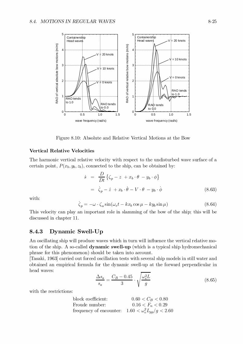
8.4. MOTIONS IN REGULAR WAVES 8-25
0
1
2
3
4
5
0 0.5 1.0 1.5
RAO tendsto 0.0
RAO tendsto 1.0
ContainershipHead waves
V = 20 knots
V = 10 knots
V = 0 knots
wave frequency (rad/s)
RA
O o
f ver
tical
abs
olut
e bo
w m
otio
ns (m
/m)
0
1
2
3
4
5
0 0.5 1.0 1.5
RAO tendsto 1.0
RAO tendsto 0.0
ContainershipHead waves
V = 0 knots
V = 10 knots
V = 20 knots
wave frequency (rad/s)
RA
O o
f ver
tical
rela
tive
bow
mot
ions
(m/m
)
Figure 8.10: Absolute and Relative Vertical Motions at the Bow
Vertical Relative Velocities
The harmonic vertical relative velocity with respect to the undisturbed wave surface of acertain point, P (xb; yb; zb), connected to the ship, can be obtained by:
_s =D
Dt
©³p ¡ z + xb ¢ µ ¡ yb ¢ Á
ª
= _³p ¡ _z + xb ¢ _µ ¡ V ¢ µ ¡ yb ¢ _Á (8.63)
with:_³p = ¡! ¢ ³a sin(!et¡ kxb cos¹¡ kyb sin¹) (8.64)
This velocity can play an important role in slamming of the bow of the ship; this will bediscussed in chapter 11.
8.4.3 Dynamic Swell-Up
An oscillating ship will produce waves which in turn will in‡uence the vertical relative mo-tion of the ship. A so-called dynamic swell-up (which is a typical ship hydromechanicalphrase for this phenomenon) should be taken into account.[Tasaki, 1963] carried out forced oscillation tests with several ship models in still water andobtained an empirical formula for the dynamic swell-up at the forward perpendicular inhead waves:
¢sasa
=CB ¡ 0:45
3¢s!2eL
g(8.65)
with the restrictions:
block coe¢cient: 0:60 < CB < 0:80Froude number: 0:16 < Fn < 0:29frequency of encounter: 1:60 < !2eLpp=g < 2:60
8-26 CHAPTER 8. FLOATING STRUCTURES IN WAVES
In this formula, sa is the amplitude of the relative motion at the forward perpendicular asobtained in head waves, calculated from the heave, the pitch and the wave motions.Then the actual amplitude of the relative motions becomes:
s¤a = sa + ¢sa (8.66)
A simple but much more fundamental method to determine the dynamic swell up forwardis given by [Journée and van ’t Veer, 1995]; it is explained here.Let an oscillating body produce damping waves, ¢³, with amplitude ¢³a. When thevertical relative motions of a point …xed to the vessel with respect to the wave elevation arecalculated, the in‡uence of the radiated damping waves must be added to the undisturbedincoming wave. Then the vertical relative motions, s, at a point, P (xb; yb), can be calculatedusing:
s(xb; yb) = ³(xb; yb) + ¢³ ¡ z(xb; yb) (8.67)
where ³ is the incoming wave elevation and z(xb; yb) is the vertical motion of the vessel inP (xb; yb) and where the radiated wave elevation is given by:
¢³ = ¢³a ¢ cos(!t¡ kjybj+ ¼) (8.68)
For zero forward speed, the amplitude ratio of the local heave motion, za(xb); at a crosssection, xb, of the body and the produced transverse radiated waves, ¢³a(xb), follows fromthe damping coe¢cient, b033(xb), and the wave speed, c = g=!:
za(xb)
¢³a(xb)=1
!¢r
½gc
b033(xb)(8.69)
This has already been discussed for an oscillating cylinder in chapter 6.Using this equation, the ratio of the amplitudes from the radiated waves due to the heavingcross section and the incoming wave becomes:
¢³a(xb)
³a=za(xb)
³a¢ ! ¢
sb033(xb)
½gc(8.70)
In case of a forward ship speed, V , the cross section is oscillating with the encounterfrequency, !e, and therefore the wave velocity, ce, of the radiated waves depends on thisfrequency:
ce =g
!e(8.71)
Due to the forward speed the radiated waves are swept back in the wake. The waveelevation at a certain point, P (xp; yp), in the ship-bounded axes system is now a result ofthe radiated waves from a cross section further ahead. The xb-position of this cross sectioncan be calculated simply, using:
xb = xp + jypj ¢ Vce
(8.72)
The amplitude of the radiated waves with a non-zero forward speed can now be calculatedusing the damping coe¢cient based on the encounter frequency and the previous expressionfor xb: ¯
¯¯¢³a(xp; yp)
³a=za(xb)
³a¢ !e ¢
sb033(xb)
½gce
¯¯¯ (8.73)
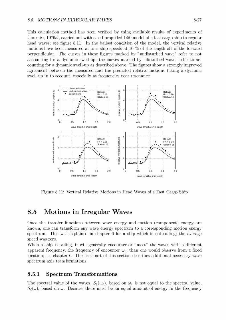
8.5. MOTIONS IN IRREGULAR WAVES 8-27
This calculation method has been veri…ed by using available results of experiments of[Journée, 1976a], carried out with a self propelled 1:50 model of a fast cargo ship in regularhead waves; see …gure 8.11. In the ballast condition of the model, the vertical relativemotions have been measured at four ship speeds at 10 % of the length aft of the forwardperpendicular. The curves in these …gures marked by ”undisturbed wave” refer to notaccounting for a dynamic swell-up; the curves marked by ”disturbed wave” refer to ac-counting for a dynamic swell-up as described above. The …gures show a strongly improvedagreement between the measured and the predicted relative motions taking a dynamicswell-up in to account, especially at frequencies near resonance.
0
2
4
6
0 0.5 1.0 1.5 2.0
BallastFn = 0.20Station 18
wave length / ship length
rela
tive
mot
ion
ampl
itude
0
2
4
6
0 0.5 1.0 1.5 2.0
BallastFn = 0.25Station 18
wave length / ship length
rela
tive
mot
ion
ampl
itude
0
2
4
6
0 0.5 1.0 1.5 2.0
BallastFn = 0.30Station 18
wave length / ship length
rela
tive
mot
ion
ampl
itude
0
2
4
6
0 0.5 1.0 1.5 2.0
disturbed waveundisturbed waveexperiment
BallastFn = 0.15Station 18
wave length / ship length
rela
tive
mot
ion
ampl
itude
Figure 8.11: Vertical Relative Motions in Head Waves of a Fast Cargo Ship
8.5 Motions in Irregular Waves
Once the transfer functions between wave energy and motion (component) energy areknown, one can transform any wave energy spectrum to a corresponding motion energyspectrum. This was explained in chapter 6 for a ship which is not sailing; the averagespeed was zero.When a ship is sailing, it will generally encounter or ”meet” the waves with a di¤erentapparent frequency, the frequency of encounter !e, than one would observe from a …xedlocation; see chapter 6. The …rst part of this section describes additional necessary wavespectrum axis transformations.
8.5.1 Spectrum Transformations
The spectral value of the waves, S³(!e), based on !e is not equal to the spectral value,S³(!), based on !. Because there must be an equal amount of energy in the frequency
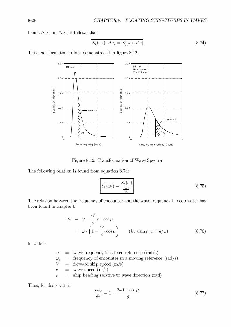
8-28 CHAPTER 8. FLOATING STRUCTURES IN WAVES
bands ¢! and ¢!e, it follows that:
jS³(!e) ¢ d!e = S³(!) ¢ d!j (8.74)
This transformation rule is demonstrated in …gure 8.12.
0
0.25
0.50
0.75
1.00
1.25
0 1 2 3
∆ω
Area = A
BF = 6
Wave frequency (rad/s)
Spe
ctra
l den
sity
(m
2 s)
0
0.25
0.50
0.75
1.00
1.25
0 1 2 3
∆ωe
Area = A
BF = 6Head wavesV = 16 knots
Frequency of encounter (rad/s)
Spe
ctra
l den
sity
(m
2s)
Figure 8.12: Transformation of Wave Spectra
The following relation is found from equation 8.74:
¯¯¯S³ (!e) =
S³ (!)d!ed!
¯¯¯ (8.75)
The relation between the frequency of encounter and the wave frequency in deep water hasbeen found in chapter 6:
!e = ! ¡ !2
gV ¢ cos¹
= ! ¢µ1¡ V
c¢ cos¹
¶(by using: c = g=!) (8.76)
in which:
! = wave frequency in a …xed reference (rad/s)!e = frequency of encounter in a moving reference (rad/s)V = forward ship speed (m/s)c = wave speed (m/s)¹ = ship heading relative to wave direction (rad)
Thus, for deep water:d!ed!
= 1¡ 2!V ¢ cos¹g
(8.77)
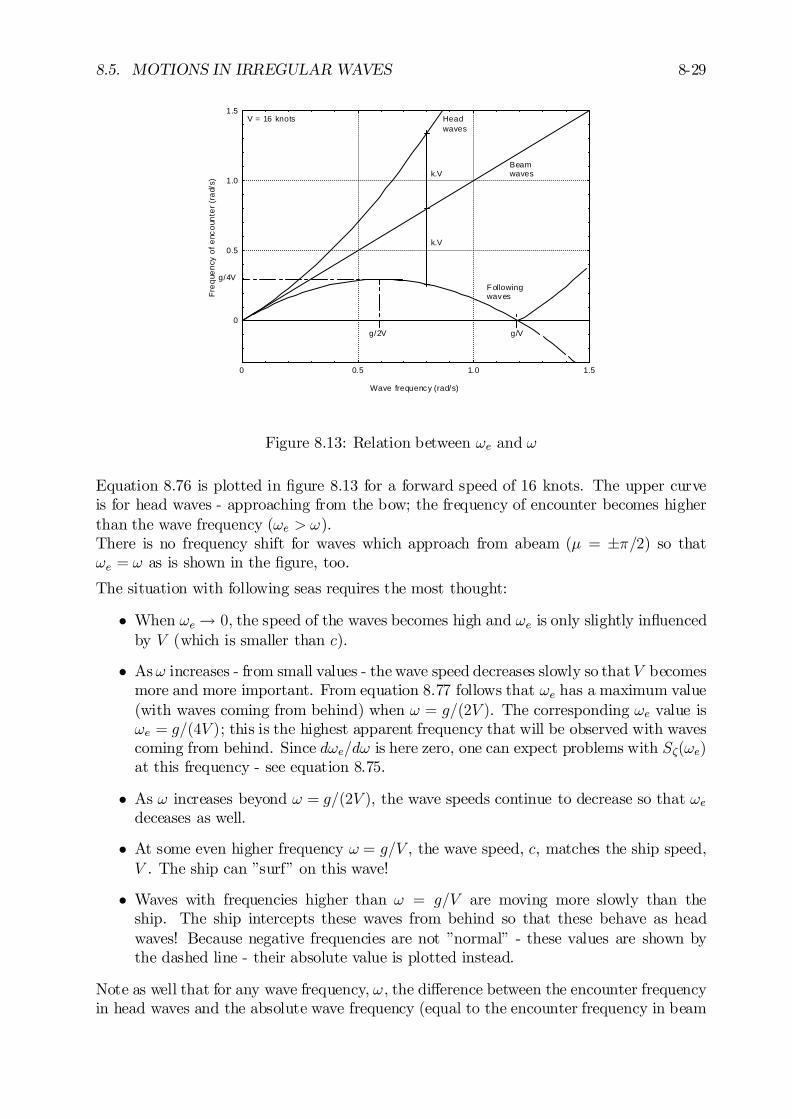
8.5. MOTIONS IN IRREGULAR WAVES 8-29
0
0.5
1.0
1.5
0 0.5 1.0 1.5
g/4V
g/2V g/V
k.V
k.V
Followingwaves
Beamwaves
Headwaves
V = 16 knots
Wave frequency (rad/s)
Freq
uenc
y of
enc
ount
er (r
ad/s
)
Figure 8.13: Relation between !e and !
Equation 8.76 is plotted in …gure 8.13 for a forward speed of 16 knots. The upper curveis for head waves - approaching from the bow; the frequency of encounter becomes higherthan the wave frequency (!e > !).There is no frequency shift for waves which approach from abeam (¹ = §¼=2) so that!e = ! as is shown in the …gure, too.
The situation with following seas requires the most thought:
² When !e ! 0, the speed of the waves becomes high and !e is only slightly in‡uencedby V (which is smaller than c).
² As! increases - from small values - the wave speed decreases slowly so that V becomesmore and more important. From equation 8.77 follows that !e has a maximum value(with waves coming from behind) when ! = g=(2V ). The corresponding !e value is!e = g=(4V ); this is the highest apparent frequency that will be observed with wavescoming from behind. Since d!e=d! is here zero, one can expect problems with S³(!e)at this frequency - see equation 8.75.
² As ! increases beyond ! = g=(2V ), the wave speeds continue to decrease so that !edeceases as well.
² At some even higher frequency ! = g=V , the wave speed, c, matches the ship speed,V . The ship can ”surf” on this wave!
² Waves with frequencies higher than ! = g=V are moving more slowly than theship. The ship intercepts these waves from behind so that these behave as headwaves! Because negative frequencies are not ”normal” - these values are shown bythe dashed line - their absolute value is plotted instead.
Note as well that for any wave frequency, !, the di¤erence between the encounter frequencyin head waves and the absolute wave frequency (equal to the encounter frequency in beam
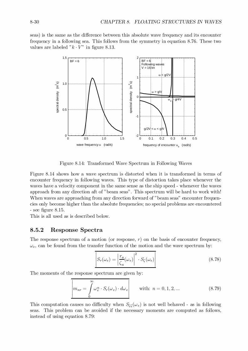
8-30 CHAPTER 8. FLOATING STRUCTURES IN WAVES
seas) is the same as the di¤erence between this absolute wave frequency and its encounterfrequency in a following sea. This follows from the symmetry in equation 8.76. These twovalues are labeled ”k ¢ V ” in …gure 8.13.
0
0.5
1.0
1.5
0 0.5 1.0 1.5
BF = 6
wave frequency ω (rad/s)
spec
tral d
ensi
ty
(m2 s)
-2
-1
0
1
2
0 0.1 0.2 0.3 0.4 0.5
ω > g/V
g/2V < ω < g/V
ω < g/2V
BF = 6Following wavesV = 16 kn
ωe = g/4V
frequency of encounter ωe (rad/s)
spec
tral d
ensi
ty
(m2 s)
Figure 8.14: Transformed Wave Spectrum in Following Waves
Figure 8.14 shows how a wave spectrum is distorted when it is transformed in terms ofencounter frequency in following waves. This type of distortion takes place whenever thewaves have a velocity component in the same sense as the ship speed - whenever the wavesapproach from any direction aft of ”beam seas”. This spectrum will be hard to work with!When waves are approaching from any direction forward of ”beam seas” encounter frequen-cies only become higher than the absolute frequencies; no special problems are encountered- see …gure 8.15.This is all used as is described below.
8.5.2 Response Spectra
The response spectrum of a motion (or response, r) on the basis of encounter frequency,!e, can be found from the transfer function of the motion and the wave spectrum by:
¯¯¯Sr(!e) =
¯¯ ra³a(!e)
¯¯2
¢ S³ (!e)¯¯¯ (8.78)
The moments of the response spectrum are given by:¯¯¯mnr =
1Z
0
!ne ¢ Sr(!e) ¢ d!e
¯¯¯ with: n = 0; 1; 2; ::: (8.79)
This computation causes no di¢culty when S³³(!e) is not well behaved - as in followingseas. This problem can be avoided if the necessary moments are computed as follows,instead of using equation 8.79:
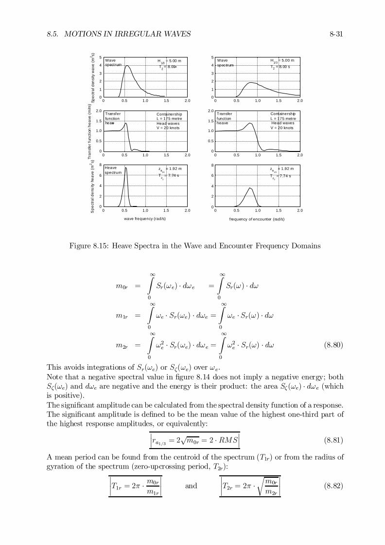
8.5. MOTIONS IN IRREGULAR WAVES 8-31
0
0.5
1.0
1.5
2.0
0 0.5 1.0 1.5 2.0
ContainershipL = 175 metre Head wavesV = 20 knots
T ransferfunct ionheave
0
1
2
3
4
5
0 0.5 1.0 1.5 2.0
Wavespec trum
H1/3
= 5.00 m
T2 = 8.00 s
0
1
2
3
4
5
0 0.5 1.0 1.5 2.0
Wavespectrum
H1/3
= 5.00 m T
2 = 8.00 s
Spec
tral d
ensi
ty w
ave
(m2 s)
0
0.5
1.0
1.5
2.0
0 0.5 1.0 1.5 2.0
ContainershipL = 175 metreHead wavesV = 20 knots
Transferfunctionheave
Tran
sfer
func
tion
heav
e (m
/m)
0
2
4
6
8
0 0.5 1.0 1.5 2.0
Heavespectrum
za1/3
= 1.92 m
Tz
2
= 7.74 s
wave frequency (rad/s)
Spe
ctra
l den
sity
hea
ve (m
2s)
0
2
4
6
8
0 0.5 1.0 1.5 2.0
za1/3
= 1.92 m
Tz2
= 7.74 s
frequency of encounter (rad/s)
Figure 8.15: Heave Spectra in the Wave and Encounter Frequency Domains
m0r =
1Z
0
Sr(!e) ¢ d!e =
1Z
0
Sr(!) ¢ d!
m1r =
1Z
0
!e ¢ Sr(!e) ¢ d!e =1Z
0
!e ¢Sr(!) ¢ d!
m2r =
1Z
0
!2e ¢ Sr(!e) ¢ d!e =1Z
0
!2e ¢ Sr(!) ¢ d! (8.80)
This avoids integrations of Sr(!e) or S³(!e) over !e.Note that a negative spectral value in …gure 8.14 does not imply a negative energy; bothS³(!e) and d!e are negative and the energy is their product: the area S³ (!e) ¢ d!e (whichis positive).The signi…cant amplitude can be calculated from the spectral density function of a response.The signi…cant amplitude is de…ned to be the mean value of the highest one-third part ofthe highest response amplitudes, or equivalently:
¯¯ra1=3 = 2
pm0r = 2 ¢RMS
¯¯ (8.81)
A mean period can be found from the centroid of the spectrum (T1r) or from the radius ofgyration of the spectrum (zero-upcrossing period, T2r):
¯¯T1r = 2¼ ¢ m0r
m1r
¯¯ and
¯¯T2r = 2¼ ¢
rm0r
m2r
¯¯ (8.82)
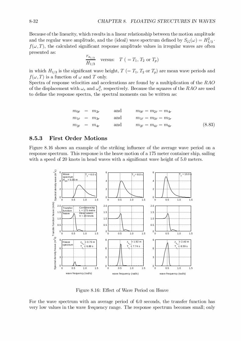
8-32 CHAPTER 8. FLOATING STRUCTURES IN WAVES
Because of the linearity, which results in a linear relationship between the motion amplitudeand the regular wave amplitude, and the (ideal) wave spectrum de…ned by S³³(!) = H2
1=3 ¢f(!; T), the calculated signi…cant response amplitude values in irregular waves are oftenpresented as:
ra1=3H1=3
versus: T ( = T1, T2 or Tp)
in which H1=3 is the signi…cant wave height, T (= T1, T2 or Tp) are mean wave periods andf(!; T) is a function of ! and T only.Spectra of response velocities and accelerations are found by a multiplication of the RAOof the displacement with !e and !2e, respectively. Because the squares of the RAO are usedto de…ne the response spectra, the spectral moments can be written as:
m0_r = m2r and m0Är = m2 _r = m4r
m1_r = m3r and m1Är = m3 _r = m5r
m2_r = m4r and m2Är = m4 _r = m6r (8.83)
8.5.3 First Order Motions
Figure 8.16 shows an example of the striking in‡uence of the average wave period on aresponse spectrum. This response is the heave motion of a 175 meter container ship, sailingwith a speed of 20 knots in head waves with a signi…cant wave height of 5.0 meters.
0
2
4
6
0 0.5 1.0 1.5
T 2 = 8.0 s
0
2
4
6
0 0.5 1.0 1.5
T2 = 10.0 s
0
0.5
1.0
1.5
2.0
0 0.5 1.0 1.5
0
3
6
9
0 0.5 1.0 1.5
za
1/3
= 2.40 m
Tz
2
= 8.59 s
wave frequency (rad/s)
0
3
6
9
0 0.5 1.0 1.5
za
1/3
= 1.92 m
Tz
2
= 7.74 s
wave frequency (rad/s )
0
0.5
1.0
1.5
2.0
0 0.5 1.0 1.5
0
2
4
6
0 0.5 1.0 1.5
T2 = 6.0 sWave
spec trumH
1/3 = 5.00 m
Spe
ctra
l den
sity
wav
e (m
2 s)
0
0.5
1.0
1.5
2.0
0 0.5 1.0 1.5
ContainershipL = 175 metreHead wavesV = 20 knots
Transferfunctionheave
Tra
nsfe
r fun
ctio
n he
ave
(m/m
)
0
3
6
9
0 0.5 1.0 1.5
H eavespectrum
za1/3
= 0.70 m
Tz
2
= 6.88 s
wave frequency (rad/s)
Spe
ctra
l den
sity
hea
ve (m
2 s)
Figure 8.16: E¤ect of Wave Period on Heave
For the wave spectrum with an average period of 6.0 seconds, the transfer function hasvery low values in the wave frequency range. The response spectrum becomes small; only
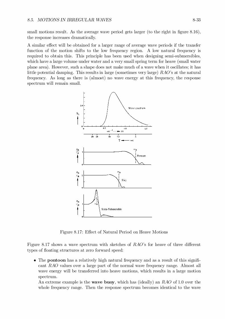
8.5. MOTIONS IN IRREGULAR WAVES 8-33
small motions result. As the average wave period gets larger (to the right in …gure 8.16),the response increases dramatically.
A similar e¤ect will be obtained for a larger range of average wave periods if the transferfunction of the motion shifts to the low frequency region. A low natural frequency isrequired to obtain this. This principle has been used when designing semi-submersibles,which have a large volume under water and a very small spring term for heave (small waterplane area). However, such a shape does not make much of a wave when it oscillates; it haslittle potential damping. This results in large (sometimes very large) RAO’s at the naturalfrequency. As long as there is (almost) no wave energy at this frequency, the responsespectrum will remain small.
Figure 8.17: E¤ect of Natural Period on Heave Motions
Figure 8.17 shows a wave spectrum with sketches of RAO’s for heave of three di¤erenttypes of ‡oating structures at zero forward speed:
² The pontoon has a relatively high natural frequency and as a result of this signi…-cant RAO values over a large part of the normal wave frequency range. Almost allwave energy will be transferred into heave motions, which results in a large motionspectrum.An extreme example is the wave buoy, which has (ideally) an RAO of 1.0 over thewhole frequency range. Then the response spectrum becomes identical to the wave
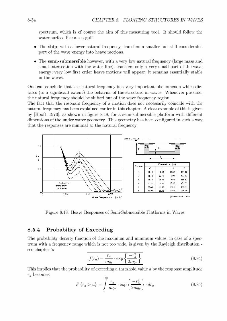
8-34 CHAPTER 8. FLOATING STRUCTURES IN WAVES
spectrum, which is of course the aim of this measuring tool. It should follow thewater surface like a sea gull!
² The ship, with a lower natural frequency, transfers a smaller but still considerablepart of the wave energy into heave motions.
² The semi-submersible however, with a very low natural frequency (large mass andsmall intersection with the water line), transfers only a very small part of the waveenergy; very low …rst order heave motions will appear; it remains essentially stablein the waves.
One can conclude that the natural frequency is a very important phenomenon which dic-tates (to a signi…cant extent) the behavior of the structure in waves. Whenever possible,the natural frequency should be shifted out of the wave frequency region.The fact that the resonant frequency of a motion does not necessarily coincide with thenatural frequency has been explained earlier in this chapter. A clear example of this is givenby [Hooft, 1970], as shown in …gure 8.18, for a semi-submersible platform with di¤erentdimensions of the under water geometry. This geometry has been con…gured in such a waythat the responses are minimal at the natural frequency.
Figure 8.18: Heave Responses of Semi-Submersible Platforms in Waves
8.5.4 Probability of Exceeding
The probability density function of the maximum and minimum values, in case of a spec-trum with a frequency range which is not too wide, is given by the Rayleigh distribution -see chapter 5: ¯
¯f(ra) =ram0r
¢ exp½ ¡r2a2m0r
¾¯¯ (8.84)
This implies that the probability of exceeding a threshold value a by the response amplitudera becomes:
P fra > ag =1Z
a
ram0r
¢ exp½ ¡r2a2m0r
¾¢ dra (8.85)
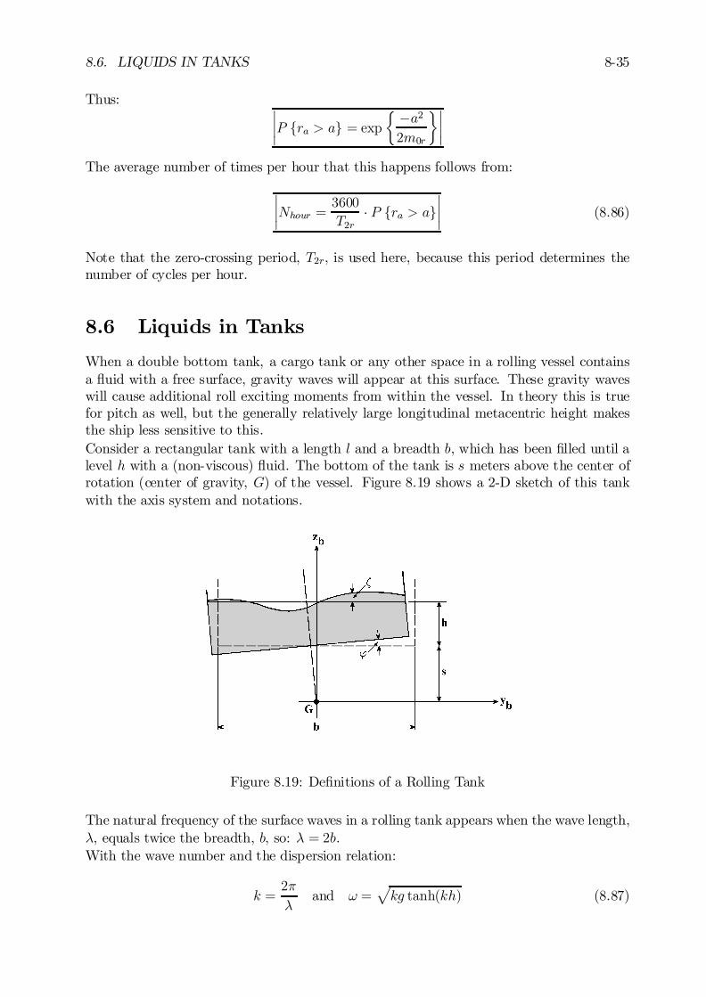
8.6. LIQUIDS IN TANKS 8-35
Thus: ¯¯P fra > ag = exp
½ ¡a22m0r
¾¯¯
The average number of times per hour that this happens follows from:
¯¯Nhour =
3600
T2r¢ P fra > ag
¯¯ (8.86)
Note that the zero-crossing period, T2r, is used here, because this period determines thenumber of cycles per hour.
8.6 Liquids in Tanks
When a double bottom tank, a cargo tank or any other space in a rolling vessel containsa ‡uid with a free surface, gravity waves will appear at this surface. These gravity waveswill cause additional roll exciting moments from within the vessel. In theory this is truefor pitch as well, but the generally relatively large longitudinal metacentric height makesthe ship less sensitive to this.Consider a rectangular tank with a length l and a breadth b, which has been …lled until alevel h with a (non-viscous) ‡uid. The bottom of the tank is s meters above the center ofrotation (center of gravity, G) of the vessel. Figure 8.19 shows a 2-D sketch of this tankwith the axis system and notations.
Figure 8.19: De…nitions of a Rolling Tank
The natural frequency of the surface waves in a rolling tank appears when the wave length,¸, equals twice the breadth, b, so: ¸ = 2b.With the wave number and the dispersion relation:
k =2¼
¸and ! =
pkg tanh(kh) (8.87)
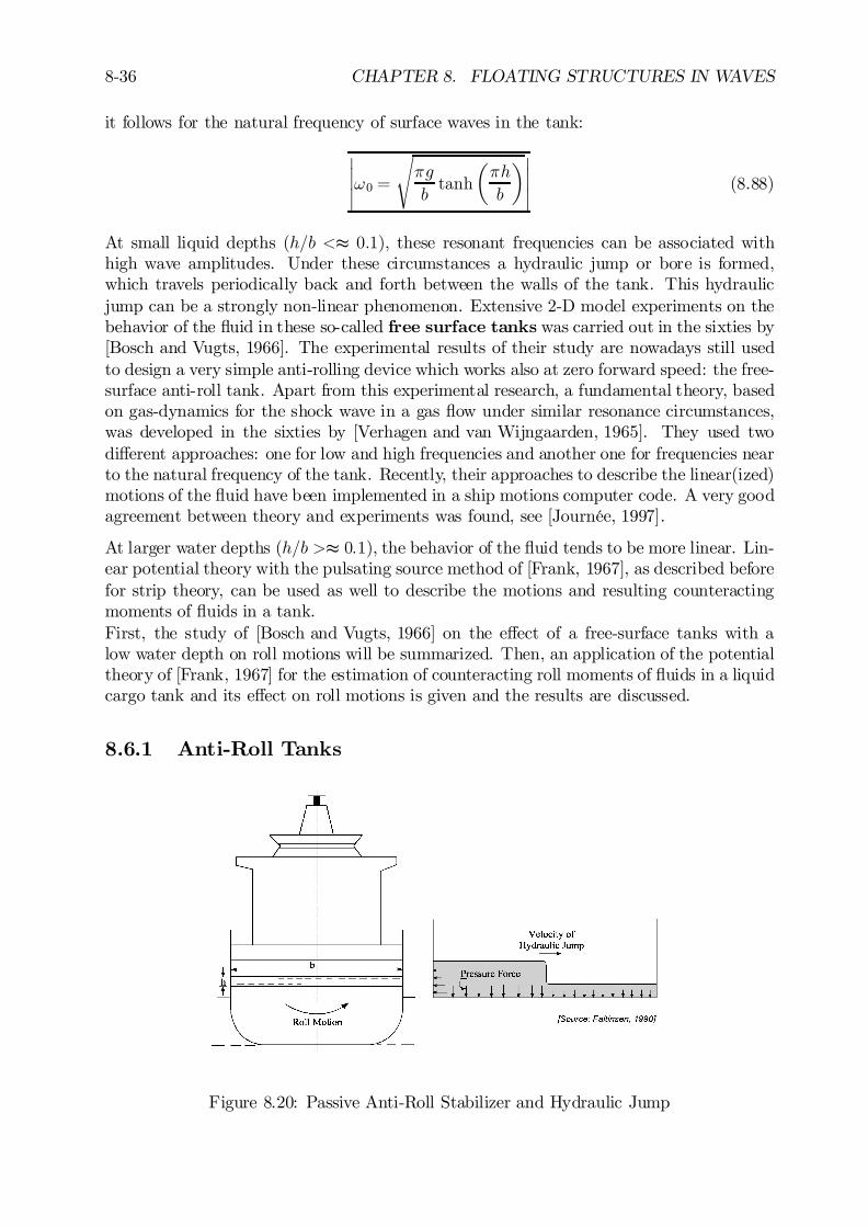
8-36 CHAPTER 8. FLOATING STRUCTURES IN WAVES
it follows for the natural frequency of surface waves in the tank:
¯¯¯!0 =
s¼g
btanh
µ¼h
b
¶¯¯¯ (8.88)
At small liquid depths (h=b <t 0:1), these resonant frequencies can be associated withhigh wave amplitudes. Under these circumstances a hydraulic jump or bore is formed,which travels periodically back and forth between the walls of the tank. This hydraulicjump can be a strongly non-linear phenomenon. Extensive 2-D model experiments on thebehavior of the ‡uid in these so-called free surface tanks was carried out in the sixties by[Bosch and Vugts, 1966]. The experimental results of their study are nowadays still usedto design a very simple anti-rolling device which works also at zero forward speed: the free-surface anti-roll tank. Apart from this experimental research, a fundamental theory, basedon gas-dynamics for the shock wave in a gas ‡ow under similar resonance circumstances,was developed in the sixties by [Verhagen and van Wijngaarden, 1965]. They used twodi¤erent approaches: one for low and high frequencies and another one for frequencies nearto the natural frequency of the tank. Recently, their approaches to describe the linear(ized)motions of the ‡uid have been implemented in a ship motions computer code. A very goodagreement between theory and experiments was found, see [Journée, 1997].
At larger water depths (h=b >t 0:1), the behavior of the ‡uid tends to be more linear. Lin-ear potential theory with the pulsating source method of [Frank, 1967], as described beforefor strip theory, can be used as well to describe the motions and resulting counteractingmoments of ‡uids in a tank.First, the study of [Bosch and Vugts, 1966] on the e¤ect of a free-surface tanks with alow water depth on roll motions will be summarized. Then, an application of the potentialtheory of [Frank, 1967] for the estimation of counteracting roll moments of ‡uids in a liquidcargo tank and its e¤ect on roll motions is given and the results are discussed.
8.6.1 Anti-Roll Tanks
Figure 8.20: Passive Anti-Roll Stabilizer and Hydraulic Jump

8.6. LIQUIDS IN TANKS 8-37
A passive free-surface tank can be a very good tool to reduce roll motions, especially atlow speeds where anti-roll …ns are not e¤ective. This tank has a breadth equal to the ship’sbreadth and its length is about 1.5 to 2.5 meter, depending on the size of the ship. The rolldamping, caused by a passive free-surface tank, is essentially based on the existence of ahydraulic jump or bore in the tank, as shown in …gure 8.20. [Bosch and Vugts, 1966] havedescribed the physical behavior of passive free-surface tanks, used as an anti-roll device.They assembled extensive quantitative information on the counteracting moments causedby the water transfer in the tank. Using their notation, the roll motions and the excitingmoments of an oscillating rectangular free-surface tank, are de…ned by:
' = 'a cos(!t)
Kt = Kta cos(!t + "t') (8.89)
In a practical frequency range, [Bosch and Vugts, 1966] have presented experimental dataon the roll moment amplitudes, Kta , and the phase shifts of these moments with respectto roll, "t, for three roll amplitudes ('a = 0:033; 0:067; 0:100 rad), four centers of rotations(¡0:40 5 s=b 5 +0:20) and …ve water depths (0:02 5 h=b 5 0:10). An example of theexperimental data is given …gure 8.21.The external roll moment due to a free surface tank, oscillating with a frequency !, canbe written as:
Kt = a4' ¢ Ä' + b4' ¢ _' + c4' ¢ ' (8.90)
with:
a4' = 0
b4' =Kta!'a
¢ sin "t'
c4' =Kta
'a¢ cos "t' (8.91)
It is obvious that for an anti-roll free-surface tank, build in the ship, the motions of shipand tank are similar:
Áa = 'a and !e = !
One can express the roll motion of the ship as well as the tank moment on the ship as:
Á = Áa cos(!et+ "Á³ )
Kt = Kta cos(!et + "Á³ + "t') (8.92)
Then, an additional exciting moment has to be added to the right hand side of the equationsof motion for roll: ¯
¯Xtank4 = a44tank ¢ ÄÁ + b44tank ¢ _Á + c44tank ¢ Á¯¯ (8.93)
with:
a44tank = 0
b44tank =Kta!eÁa
¢ sin "t' (8.94)
c44tank =KtaÁa
¢ cos "t' (8.95)
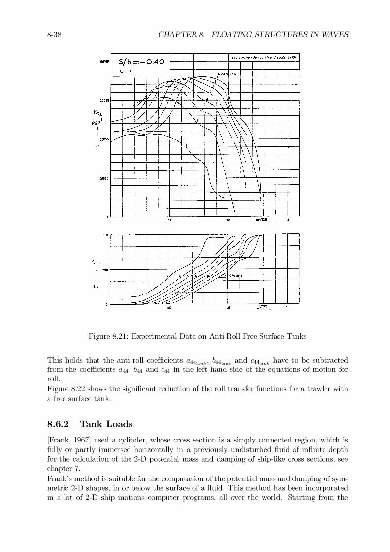
8-38 CHAPTER 8. FLOATING STRUCTURES IN WAVES
Figure 8.21: Experimental Data on Anti-Roll Free Surface Tanks
This holds that the anti-roll coe¢cients a44tank , b44tank and c44tank have to be subtractedfrom the coe¢cients a44, b44 and c44 in the left hand side of the equations of motion forroll.Figure 8.22 shows the signi…cant reduction of the roll transfer functions for a trawler witha free surface tank.
8.6.2 Tank Loads
[Frank, 1967] used a cylinder, whose cross section is a simply connected region, which isfully or partly immersed horizontally in a previously undisturbed ‡uid of in…nite depthfor the calculation of the 2-D potential mass and damping of ship-like cross sections, seechapter 7.Frank’s method is suitable for the computation of the potential mass and damping of sym-metric 2-D shapes, in or below the surface of a ‡uid. This method has been incorporatedin a lot of 2-D ship motions computer programs, all over the world. Starting from the
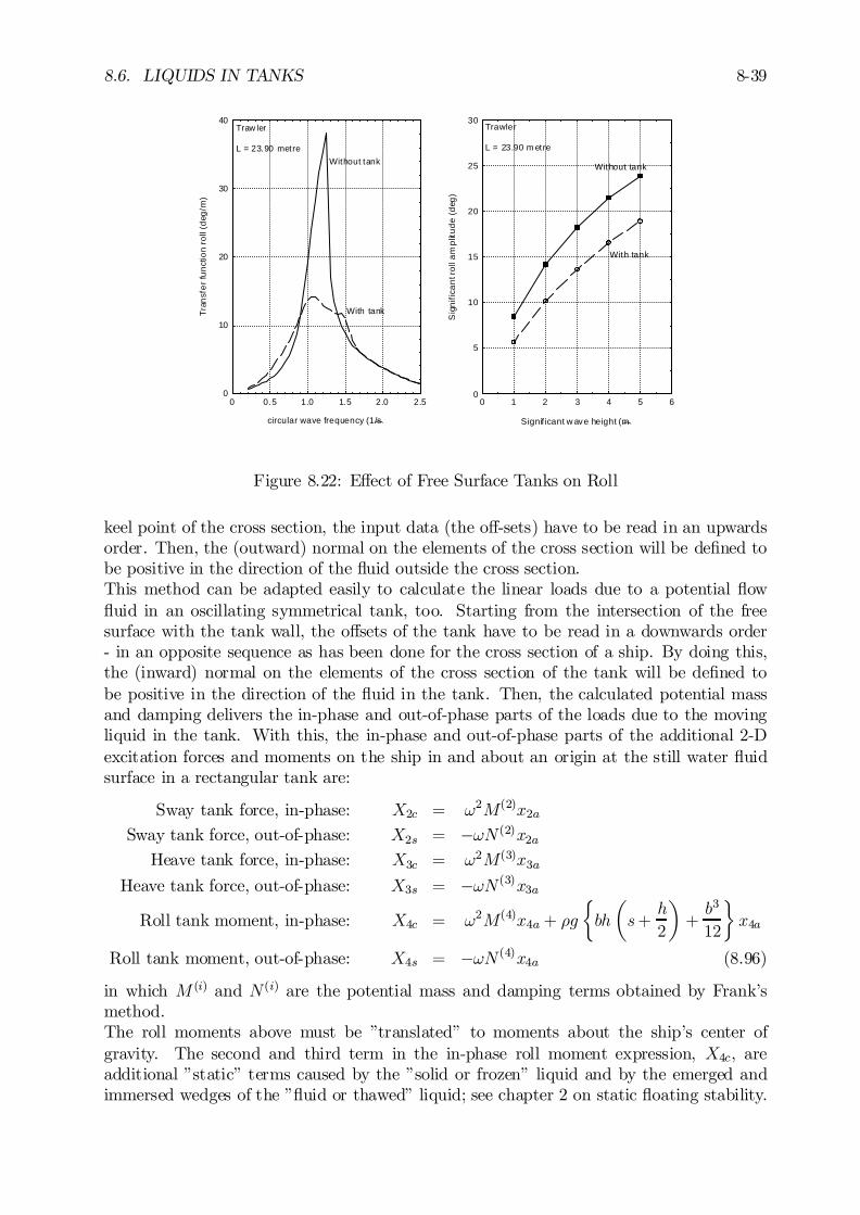
8.6. LIQUIDS IN TANKS 8-39
0
10
20
30
40
0 0.5 1.0 1.5 2.0 2.5
Traw ler L = 23.90 metre
With tank
Without tank
circular wave frequency (1/s)
Tran
sfer
func
tion
roll
(deg
/m)
0
5
10
15
20
25
30
0 1 2 3 4 5 6
Trawler L = 23.90 m etre
With tank
Without tank
Signif icant w ave height (m)
Sig
nific
ant r
oll a
mpl
itude
(de
g)
Figure 8.22: E¤ect of Free Surface Tanks on Roll
keel point of the cross section, the input data (the o¤-sets) have to be read in an upwardsorder. Then, the (outward) normal on the elements of the cross section will be de…ned tobe positive in the direction of the ‡uid outside the cross section.This method can be adapted easily to calculate the linear loads due to a potential ‡ow‡uid in an oscillating symmetrical tank, too. Starting from the intersection of the freesurface with the tank wall, the o¤sets of the tank have to be read in a downwards order- in an opposite sequence as has been done for the cross section of a ship. By doing this,the (inward) normal on the elements of the cross section of the tank will be de…ned tobe positive in the direction of the ‡uid in the tank. Then, the calculated potential massand damping delivers the in-phase and out-of-phase parts of the loads due to the movingliquid in the tank. With this, the in-phase and out-of-phase parts of the additional 2-Dexcitation forces and moments on the ship in and about an origin at the still water ‡uidsurface in a rectangular tank are:
Sway tank force, in-phase: X2c = !2M(2)x2a
Sway tank force, out-of-phase: X2s = ¡!N (2)x2aHeave tank force, in-phase: X3c = !2M(3)x3a
Heave tank force, out-of-phase: X3s = ¡!N (3)x3a
Roll tank moment, in-phase: X4c = !2M(4)x4a + ½g
½bh
µs+
h
2
¶+b3
12
¾x4a
Roll tank moment, out-of-phase: X4s = ¡!N (4)x4a (8.96)
in which M (i) and N (i) are the potential mass and damping terms obtained by Frank’smethod.The roll moments above must be ”translated” to moments about the ship’s center ofgravity. The second and third term in the in-phase roll moment expression, X4c, areadditional ”static” terms caused by the ”solid or frozen” liquid and by the emerged andimmersed wedges of the ”‡uid or thawed” liquid; see chapter 2 on static ‡oating stability.

8-40 CHAPTER 8. FLOATING STRUCTURES IN WAVES
This approach can be carried out easily with many existing 2-D, but also 3-D, ship motionscomputer programs.
Roll Moments
Forced roll oscillation experiments have been carried out with a 2-D model of a cargo tankof an LNG carrier to verify this theoretical approach. A sketch of this 1:25 model of thetank is given in …gure 8.23.
Figure 8.23: LNG Cargo Tank
The exciting roll moments have been measured for a range of oscillation frequencies anda …xed roll amplitude of 0.10 radians for several tank …lling levels. Figure 8.24 showsmeasured and predicted in-phase and out-of-phase parts of the …rst harmonic of the rollmoments of a 45 per cent …lled LNG tank as a function of the frequency of oscillation,see [Journée, 1997]. Except at the natural frequency of the ‡uid in the tank, a fairly goodprediction has been found with Frank’s 2-D pulsating source method as incorporated inthe 2-D computer program SEAWAY. Use of the 3-D computer code DELFRAC providesa similar agreement.
Roll Motions
To investigate the e¤ect of free surface (liquid cargo) tanks on the roll motions of a ship,three tanks as given in …gure 8.23 were build in a 1:60 model of an LNG carrier and equally…lled with water up to 45 % of the tank height. All other cargo tanks were assumed to be…lled up to 97.5 per cent, which was simulated in the experiments by solid ballast weightsand an adaptation of the ship’s roll radius of gyration.First, the three cargo tanks are supposed to be equally …lled up to 45 % of the tankheight with a homogeneous frozen liquid cargo with a stowage factor of 1.00 ton/m3,simulated during the experiments by solid ballast weights. The unknown radius of gyrationfor roll of the model has been obtained from free decay tests and the roll motions havebeen calculated with strip theory program SEAWAY, using the semi-empirical method of[Ikeda et al., 1978] to obtain the linearized viscous roll damping coe¢cients.Then, the cargo is ”allowed to melt”. The ship’s roll radius of gyration caused by its ownmass has been obtained from the radius of gyration of the ship with the frozen liquid cargoand a theoretical correction for thawing this cargo. The exciting roll moments due to theliquid cargo have been obtained with Frank’s method. Now, the roll motions have beencalculated, including the e¤ect of the ‡uid motions in the three tanks.
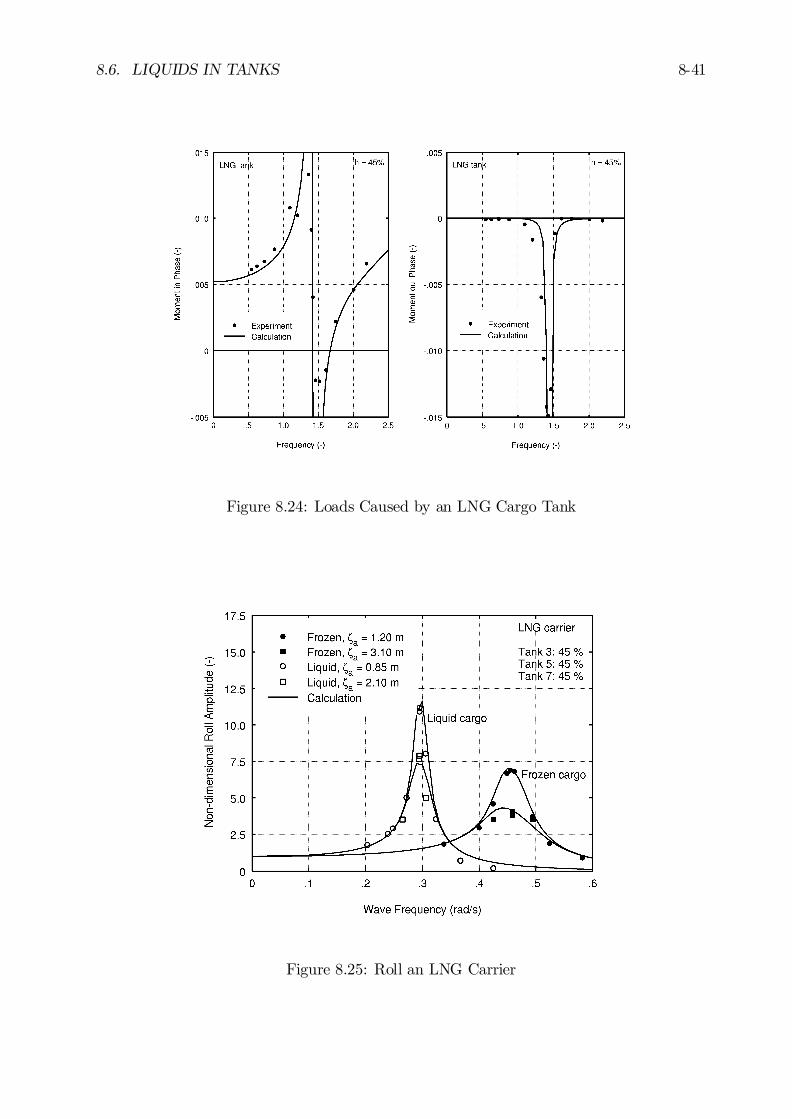
8.6. LIQUIDS IN TANKS 8-41
Figure 8.24: Loads Caused by an LNG Cargo Tank
Figure 8.25: Roll an LNG Carrier
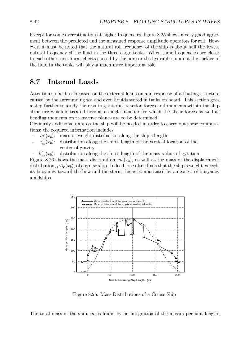
8-42 CHAPTER 8. FLOATING STRUCTURES IN WAVES
Except for some overestimation at higher frequencies, …gure 8.25 shows a very good agree-ment between the predicted and the measured response amplitude operators for roll. How-ever, it must be noted that the natural roll frequency of the ship is about half the lowestnatural frequency of the ‡uid in the three cargo tanks. When these frequencies are closerto each other, non-linear e¤ects caused by the bore or the hydraulic jump at the surface ofthe ‡uid in the tanks will play a much more important role.
8.7 Internal Loads
Attention so far has focussed on the external loads on and response of a ‡oating structurecaused by the surrounding sea and even liquids stored in tanks on board. This section goesa step further to study the resulting internal reaction forces and moments within the shipstructure which is treated here as a single member for which the shear forces as well asbending moments on transverse planes are to be determined.Obviously additional data on the ship will be needed in order to carry out these computa-tions; the required information includes:- m0(xb): mass or weight distribution along the ship’s length- z0m(xb): distribution along the ship’s length of the vertical location of the
center of gravity- k0xx(xb): distribution along the ship’s length of the mass radius of gyration
Figure 8.26 shows the mass distribution, m0(xb), as well as the mass of the displacementdistribution, ½Ax(xb), of a cruise ship. Indeed, one often …nds that the ship’s weight exceedsits buoyancy toward the bow and the stern; this is compensated by an excess of buoyancyamidships.
0
50
100
150
200
250
300
350
0 50 100 150 200
Mass distribution of the structure of the shipMass distribution of the displacem ent in st ill water
D istribut ion along Ship Length (m )
Mas
s pe
r Uni
t Len
gth
(t/m
)
Figure 8.26: Mass Distributions of a Cruise Ship
The total mass of the ship, m, is found by an integration of the masses per unit length,
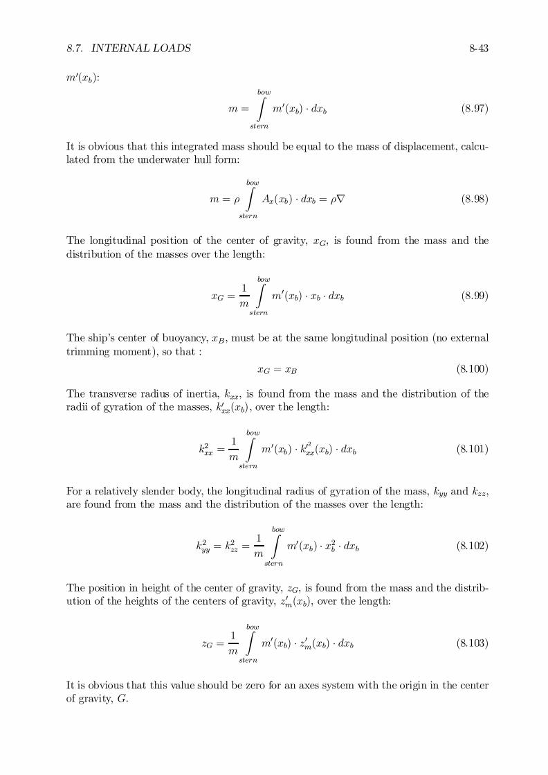
8.7. INTERNAL LOADS 8-43
m0(xb):
m =
bowZ
stern
m0(xb) ¢ dxb (8.97)
It is obvious that this integrated mass should be equal to the mass of displacement, calcu-lated from the underwater hull form:
m = ½
bowZ
stern
Ax(xb) ¢ dxb = ½r (8.98)
The longitudinal position of the center of gravity, xG, is found from the mass and thedistribution of the masses over the length:
xG =1
m
bowZ
stern
m0(xb) ¢ xb ¢ dxb (8.99)
The ship’s center of buoyancy, xB, must be at the same longitudinal position (no externaltrimming moment), so that :
xG = xB (8.100)
The transverse radius of inertia, kxx, is found from the mass and the distribution of theradii of gyration of the masses, k0xx(xb), over the length:
k2xx =1
m
bowZ
stern
m0(xb) ¢ k02xx(xb) ¢ dxb (8.101)
For a relatively slender body, the longitudinal radius of gyration of the mass, kyy and kzz,are found from the mass and the distribution of the masses over the length:
k2yy = k2zz =
1
m
bowZ
stern
m0(xb) ¢ x2b ¢ dxb (8.102)
The position in height of the center of gravity, zG, is found from the mass and the distrib-ution of the heights of the centers of gravity, z0m(xb), over the length:
zG =1
m
bowZ
stern
m0(xb) ¢ z0m(xb) ¢ dxb (8.103)
It is obvious that this value should be zero for an axes system with the origin in the centerof gravity, G.
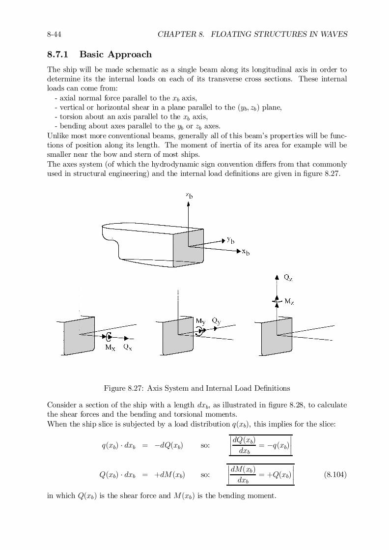
8-44 CHAPTER 8. FLOATING STRUCTURES IN WAVES
8.7.1 Basic Approach
The ship will be made schematic as a single beam along its longitudinal axis in order todetermine its the internal loads on each of its transverse cross sections. These internalloads can come from:
- axial normal force parallel to the xb axis,- vertical or horizontal shear in a plane parallel to the (yb; zb) plane,- torsion about an axis parallel to the xb axis,- bending about axes parallel to the yb or zb axes.
Unlike most more conventional beams, generally all of this beam’s properties will be func-tions of position along its length. The moment of inertia of its area for example will besmaller near the bow and stern of most ships.The axes system (of which the hydrodynamic sign convention di¤ers from that commonlyused in structural engineering) and the internal load de…nitions are given in …gure 8.27.
Figure 8.27: Axis System and Internal Load De…nitions
Consider a section of the ship with a length dxb, as illustrated in …gure 8.28, to calculatethe shear forces and the bending and torsional moments.When the ship slice is subjected by a load distribution q(xb), this implies for the slice:
q(xb) ¢ dxb = ¡dQ(xb) so:
¯¯dQ(xb)dxb
= ¡q(xb)¯¯
Q(xb) ¢ dxb = +dM (xb) so:
¯¯dM(xb)dxb
= +Q(xb)
¯¯ (8.104)
in which Q(xb) is the shear force and M (xb) is the bending moment.
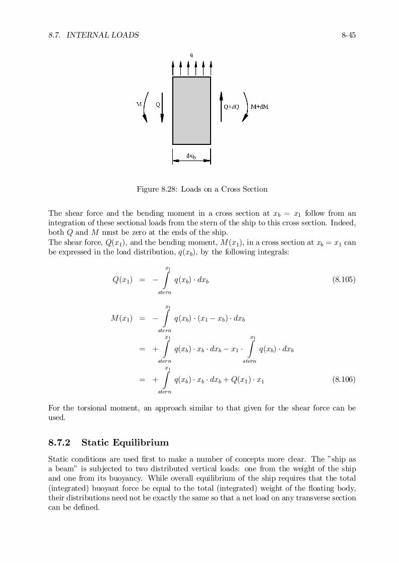
8.7. INTERNAL LOADS 8-45
Figure 8.28: Loads on a Cross Section
The shear force and the bending moment in a cross section at xb = x1 follow from anintegration of these sectional loads from the stern of the ship to this cross section. Indeed,both Q and M must be zero at the ends of the ship.The shear force, Q(x1), and the bending moment, M (x1), in a cross section at xb = x1 canbe expressed in the load distribution, q(xb), by the following integrals:
Q(x1) = ¡x1Z
stern
q(xb) ¢ dxb (8.105)
M (x1) = ¡x1Z
stern
q(xb) ¢ (x1¡ xb) ¢ dxb
= +
x1Z
stern
q(xb) ¢ xb ¢ dxb ¡ x1 ¢x1Z
stern
q(xb) ¢ dxb
= +
x1Z
stern
q(xb) ¢ xb ¢ dxb + Q(x1) ¢ x1 (8.106)
For the torsional moment, an approach similar to that given for the shear force can beused.
8.7.2 Static Equilibrium
Static conditions are used …rst to make a number of concepts more clear. The ”ship asa beam” is subjected to two distributed vertical loads: one from the weight of the shipand one from its buoyancy. While overall equilibrium of the ship requires that the total(integrated) buoyant force be equal to the total (integrated) weight of the ‡oating body,their distributions need not be exactly the same so that a net load on any transverse sectioncan be de…ned.
8-46 CHAPTER 8. FLOATING STRUCTURES IN WAVES
Consider the forces acting on a section of the ship with a length dxb. The vertical forceson a transverse ’slice’ of a ship in still water are given by:
(m0 ¢ dxb) ¢ (¡g) = qz(xb) ¢ dxb (8.107)
in which:jqz(xb) = f½ ¢ Ax(xb) ¡m0(xb)g ¢ gj (8.108)
where Ax is the cross sectional area.With equations 8.105 and 8.106, the vertical shear force, Qz(x1), and the bending moment,My(x1), in still water in a cross section can be obtained from the vertical load, qx(xb), bythe following integrals:
¯¯¯Qz(x1) = ¡
x1Z
stern
qz(xb) ¢ dxb
¯¯¯
¯¯¯My(x1) = +
x1Z
stern
qz(xb) ¢ xb ¢ dxb + Qz(x1) ¢ x1
¯¯¯ (8.109)
Figure 8.29 shows an example of a calculated still water bending moment, My, curve of acruise ship with a weight and buoyancy distribution as given in …gure 8.26.
0
0.25x10⁶
0.50x10⁶
0.75x10⁶
1.00x10⁶
1.25x10⁶
0 50 100 150 200
Distribution Along Ship Length (m)
Stil
l Wat
er B
endi
ng M
omen
t (k
Nm
)
Figure 8.29: Distribution of Still Water Bending Moments of a Cruise Ship
The generally positive moment here is common in ships. As used here, a positive momentimplies that the bow and stern of the ship tend to bend down. This if often called hogging;the opposite tendency is called sagging.Still water bending moments can become signi…cant. A well-known example of some yearsago is the supertanker Energy Concentration moored in Europoort. It su¤ered the con-sequences of completely emptying the amidships cargo tanks while the fore and aft tanks
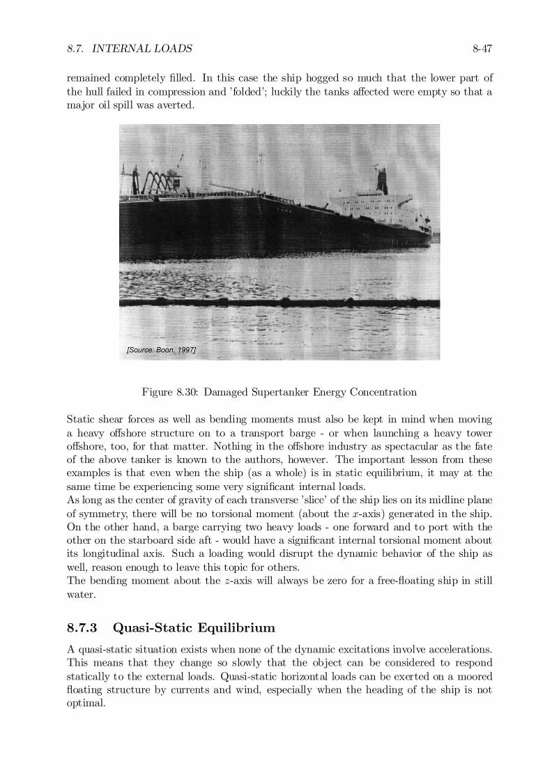
8.7. INTERNAL LOADS 8-47
remained completely …lled. In this case the ship hogged so much that the lower part ofthe hull failed in compression and ’folded’; luckily the tanks a¤ected were empty so that amajor oil spill was averted.
Figure 8.30: Damaged Supertanker Energy Concentration
Static shear forces as well as bending moments must also be kept in mind when movinga heavy o¤shore structure on to a transport barge - or when launching a heavy towero¤shore, too, for that matter. Nothing in the o¤shore industry as spectacular as the fateof the above tanker is known to the authors, however. The important lesson from theseexamples is that even when the ship (as a whole) is in static equilibrium, it may at thesame time be experiencing some very signi…cant internal loads.As long as the center of gravity of each transverse ’slice’ of the ship lies on its midline planeof symmetry, there will be no torsional moment (about the x-axis) generated in the ship.On the other hand, a barge carrying two heavy loads - one forward and to port with theother on the starboard side aft - would have a signi…cant internal torsional moment aboutits longitudinal axis. Such a loading would disrupt the dynamic behavior of the ship aswell, reason enough to leave this topic for others.The bending moment about the z-axis will always be zero for a free-‡oating ship in stillwater.
8.7.3 Quasi-Static Equilibrium
A quasi-static situation exists when none of the dynamic excitations involve accelerations.This means that they change so slowly that the object can be considered to respondstatically to the external loads. Quasi-static horizontal loads can be exerted on a moored‡oating structure by currents and wind, especially when the heading of the ship is notoptimal.

8-48 CHAPTER 8. FLOATING STRUCTURES IN WAVES
The ship is now a beam (when seen from above) which has a location-dependent distributedload and concentrated reaction forces (similar to the supports of a conventional beam) atthe mooring line attachment points. Otherwise, the analysis is much like that for the staticvertical load case handled above. In general the ends of the ship are still ’free’ so that boththe horizontal crosswise shear, Qy, and moment, Mz, will be zero at each end of the ship.
There is more to this that has not yet been considered, however! In general the horizontalforces from the anchor lines, the transverse wind loads and the transverse current loadswill not all act at the same elevation; the various forces will act at di¤erent elevations inthe (x; z) plane. This has two consequences.As a whole, the ‡oating body will generally come to a static roll angle so that any imbalanceof the externally caused external moments will be held in equilibrium by a static rollmoment. A good example of this is how a sailboat with the wind on the beam will heelas a result of the wind load in one direction on the sails and the lateral hydrodynamicresistance of the hull working in the other direction; see …gure 8.31.
Figure 8.31: Lateral Forces on a Sailboat
Even though this static roll moment will bring the sailboat (in this example) into over-all equilibrium, internal torsional moments will generally still exist. Indeed, with mostsailboats, the entire moment from the sail is transferred to the hull at the cross-sectionwhere the mast is located. This moment can be distributed to the rest of the hull only viatorsional moments about the ship’s x-axis.Quasi-static axial forces can be present in a ship which is sailing (not necessarily a sailboatnow), too. The force driving the ship forward (from the propeller) is transferred via itsshaft to a thrust bearing where this load is transferred to the hull. The hull forward ofthis location is obviously ’pushed’ through the water; there will obviously be a compressivenormal stress in the ship sections forward of the thrust bearing. By the same reasoning,all ship sections aft of the thrust bearing will be under a slight tension as the after bodyof the ship is pulled through the water.
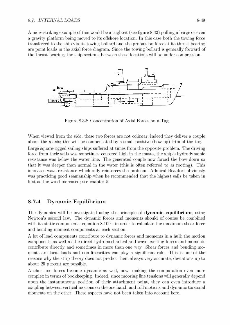
8.7. INTERNAL LOADS 8-49
A more striking example of this would be a tugboat (see …gure 8.32) pulling a barge or evena gravity platform being moved to its o¤shore location. In this case both the towing forcetransferred to the ship via its towing bollard and the propulsion force at its thrust bearingare point loads in the axial force diagram. Since the towing bollard is generally forward ofthe thrust bearing, the ship sections between these locations will be under compression.
Figure 8.32: Concentration of Axial Forces on a Tug
When viewed from the side, these two forces are not colinear; indeed they deliver a coupleabout the y-axis; this will be compensated by a small positive (bow up) trim of the tug.
Large square-rigged sailing ships su¤ered at times from the opposite problem. The drivingforce from their sails was sometimes centered high in the masts, the ship’s hydrodynamicresistance was below the water line. The generated couple now forced the bow down sothat it was deeper than normal in the water (this is often referred to as rooting). Thisincreases wave resistance which only reinforces the problem. Admiral Beaufort obviouslywas practicing good seamanship when he recommended that the highest sails be taken in…rst as the wind increased; see chapter 5.
8.7.4 Dynamic Equilibrium
The dynamics will be investigated using the principle of dynamic equilibrium, usingNewton’s second law. The dynamic forces and moments should of course be combinedwith its static component - equation 8.109 - in order to calculate the maximum shear forceand bending moment components at each section.
A lot of load components contribute to dynamic forces and moments in a hull; the motioncomponents as well as the direct hydromechanical and wave exciting forces and momentscontribute directly and sometimes in more than one way. Shear forces and bending mo-ments are local loads and non-linearities can play a signi…cant role. This is one of thereasons why the strip theory does not predict them always very accurate; deviations up toabout 25 percent are possible.
Anchor line forces become dynamic as well, now, making the computation even morecomplex in terms of bookkeeping. Indeed, since mooring line tensions will generally dependupon the instantaneous position of their attachment point, they can even introduce acoupling between vertical motions on the one hand, and roll motions and dynamic torsionalmoments on the other. These aspects have not been taken into account here.

8-50 CHAPTER 8. FLOATING STRUCTURES IN WAVES
Lateral Dynamic Loads
Consider the horizontal forces acting on a section of the ship with a length dxb. Accordingto Newton’s second law, the harmonic lateral dynamic load per unit length on a transverse’slice’ of the ship is given by:
qy(xb) = +X 0hy(xb) +X
0wy(xb)
+½gAx(xb) ¢ Á¡m0(xb) ¢
nÄy + xb ¢ ÄÃ ¡ z0m ¢ ÄÁ + g ¢ Á
o(8.110)
where Ax(xb) is the sectional area, X 0hy(xb) and X 0
wy(xb) are the sectional hydromechanicaland wave forces for sway and m0gÁ is the lateral mass-force component due to the de…nitionof the lateral loads in the ship-bound axes system, respectively.With equations 8.105 and 8.106, the harmonic lateral shear force, Qy(x1), and the bendingmoment, Mz(x1), in waves in cross section x1 can be obtained from the horizontal load,qy(xb), by the following integrals:
¯¯¯Qy(x1) = Qya cos(!et + "Qz³) = ¡
x1Z
stern
qy(xb) ¢ dxb
¯¯¯
¯¯¯Mz(x1) =Mza cos(!et+ "Mz³) = ¡
x1Z
stern
qy(xb) ¢ xb ¢ dxb ¡Qy(x1) ¢ x1
¯¯¯ (8.111)
Vertical Dynamic Loads
Consider the vertical forces acting on a section of the ship with a length dxb. Accordingto Newton’s second law, the harmonic longitudinal and vertical dynamic forces per unitlength on a transverse ’slice’ of the ship are given by:
qx(xb) = +X 0hx(xb) +X
0wx(xb) ¡m0(xb) ¢
nÄx¡ bG(xb) ¢ ĵ
o
qz(xb) = +X 0hz(xb) +X
0wz(xb) ¡m0(xb) ¢
nÄz ¡ xb ¢ ĵ
o(8.112)
where bG(xb) is the distance of the centroid of the cross section to the xb axis andX 0hx(xb); X
0hz(xb) and X 0
wx(xb); X0wz(xb) are the sectional hydromechanical and wave forces
for surge and heave, respectively.With equations 8.105 and 8.106, the harmonic vertical shear force, Qz(x1), and the bendingmoment, My(x1), in waves in cross section x1 can be obtained from the longitudinal andvertical loads, qx(xb) and qz(xb), by the following integrals:
¯¯¯Qz(x1) = Qza cos(!et + "Qz³ ) = ¡
x1Z
stern
qz(xb) ¢ dxb
¯¯¯
¯¯¯My(x1) =Mya cos(!et+ "My³) = +
x1Z
stern
qx(xb) ¢ bG(xb) ¢ dxb
¯¯¯

8.7. INTERNAL LOADS 8-51
¯¯¯ +
x1Z
stern
qz(xb) ¢ xb ¢ dxb + Qz(x1) ¢ x1
¯¯¯ (8.113)
Figure 8.33 shows a comparison between measured and calculated distribution of the ver-tical wave bending moment amplitudes over the length of the ship
Figure 8.33: Distribution of Vertical Bending Moment Amplitudes
Torsional Dynamic Loads
Consider the moments acting on a section of the ship with a length dxb. According toNewton’s second law, the harmonic torsional dynamic moment per unit length on a trans-verse ’slice’ of the ship about a longitudinal axis at a distance z1 above the ship’s centerof gravity is given by:
qÁ(xb; z1) = +X 0hÁ(xb) +X
0wÁ(xb) (8.114)
+z1 ¢ qy(xb) ¡m0(xb) ¢nk02
xx ¢ ÄÁ¡ z0m ¢ (Äy + xb ¢ ÄÃ + g ¢ Á)o
where X 0hÁ(xb) and X 0
wÁ(xb) are the sectional hydromechanical and wave moments for roll,respectively.With equation 8.105, the harmonic torsional moment, Mx(x1; z1), in waves in cross sectionx1 at a distance z1 above the ship’s center of gravity can be obtained from the torsionalloads, qÁ(xb; z1), by the following integral:
¯¯¯Mx(x1; z1) =Mxa cos(!et + "Mx³) = ¡
x1Z
stern
qÁ(xb; z1) ¢ dxb
¯¯¯ (8.115)
It is important to realize, for example, that a ship sailing in quartering waves -approachingfrom about 45 degrees o¤ the stern - can experience very signi…cant dynamic torsionalmoments - even if it is not rolling very much. Both the wave direction (and associatedrelative phases along the ship’s axis) and the low frequency of encounter contribute to alarge transfer function value in this case.
8-52 CHAPTER 8. FLOATING STRUCTURES IN WAVES
8.7.5 Internal Loads Spectra
The internal loads spectra can be calculated in a way similar to that described earlier forother harmonic responses.
8.7.6 Fatigue Assessments
It has already been pointed out that the transfer functions for any of the above forcescan be computed by carefully (and properly!) superposing the components for the alreadyknown functions for forces and ship motions. One can go even deeper into the structuralengineering aspects, however as long as the system remains linear in its behavior.Knowing all six of the load components on a ship cross-section, a marine structural engineercan - knowing a lot more details of the internal structure of the ship - convert each of theseforces to associated stress components. Stress concentration factors and other details mustnow be taken into account along the way, of course.These stress components can in turn be combined to determine principal stresses and evento carry out a fatigue analysis. Structural engineering and o¤shore hydromechanics areoften very closely linked - if not married - within o¤shore engineering! This will show upagain when sea fastening of o¤shore structures to transport barges is discussed in chapter11.Fatigue analyses depend upon two independent input data items:
- Magnitude of the (local) stress change - stress range.- Associated number of cycles with this stress range.
This information can then be combined using the Miner-Palmgren rule to obtain an overallfatigue damage estimate. The structural analysis details of this are left to others moreexpert in this …eld, but a bit more about each of the above two items is discussed here.The magnitude of the stress change within a ship or other large structure will be linearlyrelated to the ambient waves. If the object has a …xed location, then wave climate datais relatively easy to obtain and work with. Even if the object is only seasonally, one canapproach the wave data in a quite straight forward way - see chapter 5.More ”portable” objects - such as a major pipe laying vessel that may spend some timenear Australia before going to the west coast of Africa before coming to the North sea fora while - present a formidable bookkeeping problem. If the problem to be solved involvesthe determination of the ”remaining fatigue life” of an existing vessel, then obtaining thecumulative - location and time dependent - wave climate presents a signi…cant problem.The pragmatic solution in a design situation, on the other hand, would be to determinefatigue life based upon continuous exposure to some de…ned wave climate such as that forthe northern North Sea.
Global and Local Loads
Fatigue sensitive locations in a vessel are the deck, bottom and possibly the sides-shell.The loads important for fatigue can be split in global and local loads. Global loads areloads in a cross section of the hull girder and make equilibrium with the ”accelerationforces” due to the motions and the pressure integration over the speci…c hull section; thesehave been determined above. Local internal loads result from pressures at speci…c spotson the hull inducing additional locally ‡uctuating stresses. The simple e¤ect of external
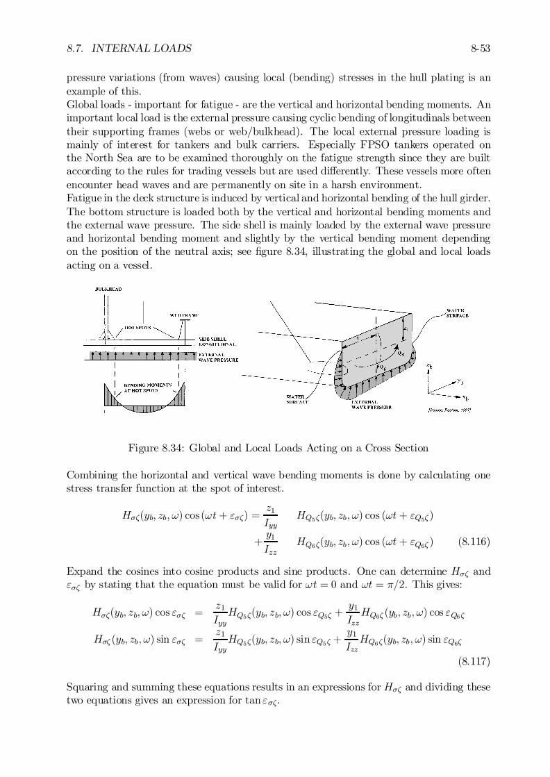
8.7. INTERNAL LOADS 8-53
pressure variations (from waves) causing local (bending) stresses in the hull plating is anexample of this.Global loads - important for fatigue - are the vertical and horizontal bending moments. Animportant local load is the external pressure causing cyclic bending of longitudinals betweentheir supporting frames (webs or web/bulkhead). The local external pressure loading ismainly of interest for tankers and bulk carriers. Especially FPSO tankers operated onthe North Sea are to be examined thoroughly on the fatigue strength since they are builtaccording to the rules for trading vessels but are used di¤erently. These vessels more oftenencounter head waves and are permanently on site in a harsh environment.Fatigue in the deck structure is induced by vertical and horizontal bending of the hull girder.The bottom structure is loaded both by the vertical and horizontal bending moments andthe external wave pressure. The side shell is mainly loaded by the external wave pressureand horizontal bending moment and slightly by the vertical bending moment dependingon the position of the neutral axis; see …gure 8.34, illustrating the global and local loadsacting on a vessel.
Figure 8.34: Global and Local Loads Acting on a Cross Section
Combining the horizontal and vertical wave bending moments is done by calculating onestress transfer function at the spot of interest.
H¾³(yb; zb; !) cos(!t+ "¾³) =z1Iyy
HQ5³(yb; zb; !) cos (!t+ "Q5³ )
+y1Izz
HQ6³(yb; zb; !) cos (!t+ "Q6³ ) (8.116)
Expand the cosines into cosine products and sine products. One can determine H¾³ and"¾³ by stating that the equation must be valid for !t = 0 and !t = ¼=2. This gives:
H¾³(yb; zb; !) cos "¾³ =z1IyyHQ5³(yb; zb; !) cos "Q5³ +
y1IzzHQ6³ (yb; zb; !) cos "Q6³
H¾³ (yb; zb; !) sin "¾³ =z1IyyHQ5³(yb; zb; !) sin "Q5³ +
y1IzzHQ6³(yb; zb; !) sin "Q6³
(8.117)
Squaring and summing these equations results in an expressions forH¾³ and dividing thesetwo equations gives an expression for tan "¾³.
8-54 CHAPTER 8. FLOATING STRUCTURES IN WAVES
The external pressure can be incorporated as well for those position which are alwayswet - the bottom and bilges. In this case a pressure transfer function is required alongwith a structural model to determine the local stress contribution - just as is neededfor the global internal loads as well. Side shell loading is more complicated. Since thewater surface is ‡uctuating the side shell is sometimes wet and sometimes dry. Hence thisloading is strongly nonlinear which is di¢cult to account for properly. For calculationroutines and ways to combine this nonlinear load with the global loads one is referred to[Cramer and et.al., 1993], [Pastoor, 1997b] and [Pastoor, 1997a].
Once the proper overall transfer functions and some form of cumulative wave scatter dia-gram has been determined, each of its ”cells” - with its own characteristic wave height andperiod - can be transformed to:
² A characteristic stress variation dependent upon the waves and a whole ”chain” oftransfer functions.
² A number of stress variation cycles dependent upon the wave period and the numberof observations associated with that wave scatter diagram cell.
Often several adjacent cells in the wave scatter diagram are combined when carrying outthis transformation.Once this procedure has been followed for all wave scatter diagram cells, one can sum upthe results in order to obtain the input data for a Miner-Palmgren sum.
8.8 Added Resistance in Waves
A ship moving forward in a wave …eld will generate ”two sets of waves”: waves associatedwith forward speed through still water and waves associated with its vertical relative motionresponse to waves. Since both wave patterns dissipate energy, it is logical to conclude thata ship moving through still water will dissipate less energy than one moving through waves.The extra wave-induced loss of energy can be treated as an added propulsion resistance -see chapter 4.Figure 8.35 shows the resistance in regular waves as a function of the time: a constantpart due the calm water resistance and an oscillating part due to the motions of the ship,relative to the incoming regular waves. The time-averaged part of the increase of resistanceis called: the added resistance due to waves, Raw.Two theoretical methods for the estimation of the time-averaged added resistance of a shipdue to its vertical motions relative to the waves are described here:
² a radiated wave energy methodintroduced by [Gerritsma and Beukelman, 1972] and suitable for head to beam waves
² an integrated pressure methodintroduced by [Boese, 1970] and suitable for all wave directions.
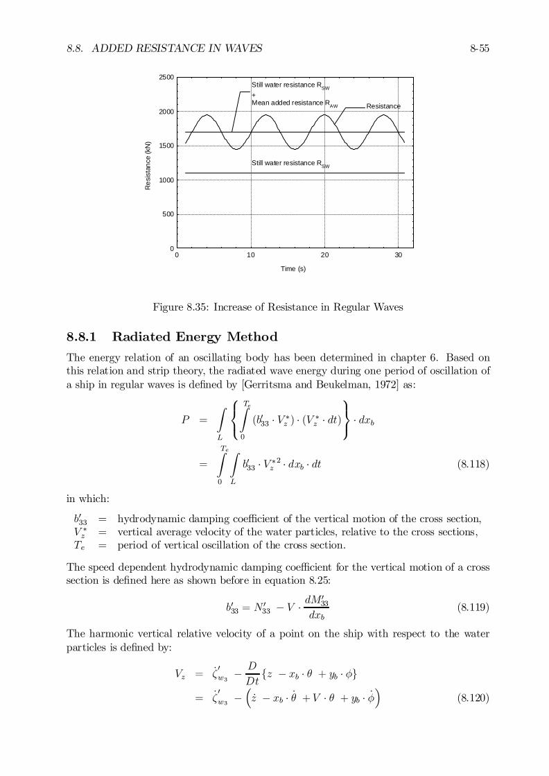
8.8. ADDED RESISTANCE IN WAVES 8-55
0
500
1000
1500
2000
2500
0 10 20 30
Resistance
Still water resistance RSW
+Mean added resistance RAW
Still water resistance RSW
Time (s)
Res
ista
nce
(kN
)
Figure 8.35: Increase of Resistance in Regular Waves
8.8.1 Radiated Energy Method
The energy relation of an oscillating body has been determined in chapter 6. Based onthis relation and strip theory, the radiated wave energy during one period of oscillation ofa ship in regular waves is de…ned by [Gerritsma and Beukelman, 1972] as:
P =
Z
L
8<:
TeZ
0
(b033 ¢ V ¤z ) ¢ (V ¤z ¢ dt)
9=; ¢ dxb
=
TeZ
0
Z
L
b033 ¢ V ¤z 2 ¢ dxb ¢ dt (8.118)
in which:
b033 = hydrodynamic damping coe¢cient of the vertical motion of the cross section,V ¤z = vertical average velocity of the water particles, relative to the cross sections,Te = period of vertical oscillation of the cross section.
The speed dependent hydrodynamic damping coe¢cient for the vertical motion of a crosssection is de…ned here as shown before in equation 8.25:
b033 = N033 ¡ V ¢ dM
033
dxb(8.119)
The harmonic vertical relative velocity of a point on the ship with respect to the waterparticles is de…ned by:
Vz = _³0w3
¡ D
Dtfz ¡ xb ¢ µ + yb ¢ Ág
= _³0w3 ¡
³_z ¡ xb ¢ _µ + V ¢ µ + yb ¢ _Á
´(8.120)
8-56 CHAPTER 8. FLOATING STRUCTURES IN WAVES
For a cross section of the ship, an equivalent harmonic vertical relative velocity has to befound. This equivalent relative velocity is de…ned by:
V ¤z = _³¤w3
¡³_z ¡ xb ¢ _µ + V ¢ µ
´
= V ¤za ¢ cos(!et+ "V ¤z ³ ) (8.121)
With this the radiated energy during one period of oscillation is given by:
P =¼
!e
Z
L
µN 033 ¡ V ¢ dM
033
dxb
¶¢ V ¤za2 ¢ dxb (8.122)
To maintain a constant forward ship speed, this energy should be provided by the ship’spropulsion plant. A mean added resistance, Raw, has to be gained. The energy providedto the surrounding water is given by:
P = Raw ¢µV ¡ c
cos¹
¶¢ Te
= Raw ¢ 2¼
¡k cos¹ (8.123)
From this the transfer function of the mean added resistance according to Gerritsma andBeukelman can be found:
¯¯¯Raw³2a
=¡k cos¹2!e
¢Z
L
µN 033 ¡ V ¢ dM
033
dxb
¶¢µV ¤za³a
¶2¢ dxb
¯¯¯ (8.124)
This method gives good results in head to beam waves. However, this method fails infollowing waves. When the wave speed in following waves approaches the ship speed thefrequency of encounter in the denominator tends to zero. At these low frequencies, thepotential sectional mass is very high and the potential sectional damping is almost zero.The damping multiplied with the relative velocity squared in the numerator does not tendto zero, as fast as the frequency of encounter. This is caused by the presence of a naturalfrequency for heave and pitch at this low !e, so a high motion peak can be expected. Thisresults in extreme (positive and negative) added resistances.
8.8.2 Integrated Pressure Method
[Boese, 1970] calculates the added resistance by integrating the longitudinal components ofthe oscillating pressures on the wetted surface of the hull. A second small contribution ofthe longitudinal component of the vertical hydrodynamic and wave forces has been added.The wave elevation is given by:
³ = ³a cos(!et ¡ kxb cos¹¡ kyb sin¹) (8.125)
The pressure in the undisturbed waves in deep water is given by:
p = ¡½gz + ½g ¢ ekz³ (8.126)
8.8. ADDED RESISTANCE IN WAVES 8-57
The horizontal force on an oscillating cross section is given by:
f(xb; t) =
³Z
¡Ds+zx
p dzb with: zx = z ¡ xbµ (8.127)
As the mean added resistance during one period will be calculated, the constant term andthe …rst harmonic term can be ignored, so:
f ¤(xb; t) = ¡12½g
©³2 ¡ (¡Ds + zx)2
ª
= ¡12½g (³ ¡ zx)2 (8.128)
The vertical relative motion is de…ned by s = ³ ¡ zx, so:
f ¤(xb; t) = ¡12½g s2 (8.129)
The average horizontal force on a cross section follows from:
f¤(xb) =
TeZ
0
f¤(xb; t) dt =1
4½g s2a (8.130)
The added resistance due to this force is:
Raw1 = 2
Z
L
f¤(xb)µ
¡dywdxb
¶dxb (8.131)
so that this part of the mean added resistance reduces to:
Raw1 = ¡12½g
Z
L
s2adywdxb
dxb (8.132)
The integrated vertical hydromechanical and wave forces in the ship bounded axis systemvaries not only in time but also in direction with the pitch angle. From this follows asecond contribution to the mean added resistance:
Raw2 =¡1Te
T eZ
0
fXh3(t) +Xw3 (t)g µ(t) dt
=¡1Te
T eZ
0
½r Äz(t) µ(t) dt (8.133)
This second contribution can be written as:
Raw2 =1
2½r !2e za µa cos("z³ ¡ "µ³) (8.134)
so that the transfer function of the total mean added resistance according to Boese is givenby: ¯
¯¯Raw
³2a=1
2½g
Z
L
µsa³a
¶2 dywdxb
dxb +1
2½r !2e
za³a
µa³acos("z³ ¡ "µ³)
¯¯¯ (8.135)
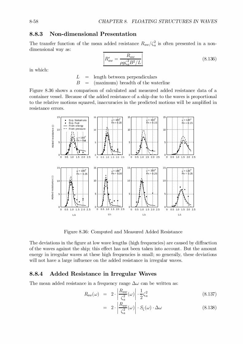
8-58 CHAPTER 8. FLOATING STRUCTURES IN WAVES
8.8.3 Non-dimensional Presentation
The transfer function of the mean added resistance Raw=³2a is often presented in a non-dimensional way as: ¯
¯R 0aw =Raw
½g³2aB2=L
¯¯ (8.136)
in which:
L = length between perpendicularsB = (maximum) breadth of the waterline
Figure 8.36 shows a comparison of calculated and measured added resistance data of acontainer vessel. Because of the added resistance of a ship due to the waves is proportionalto the relative motions squared, inaccuracies in the predicted motions will be ampli…ed inresistance errors.
0
5
10
15
0 0. 5 1.0 1 .5 2.0 2.5
µ = 180o
Fn = 0.20
0
5
10
15
0 0.5 1.0 1.5 2.0 2.5
µ = 150o
Fn = 0.15
0
5
10
15
0 0.5 1.0 1.5 2.0 2.5
µ = 120o
Fn = 0.15
0
5
10
15
0 0.5 1.0 1.5 2.0 2.5
µ = 180o
Fn = 0.25
L/λ
Adde
d re
sist
ance
(-)
0
5
10
15
0 0.5 1.0 1.5 2.0 2.5
µ = 180o
Fn = 0.30
L/λ
0
5
10
15
0 0.5 1.0 1.5 2.0 2.5
µ = 150o
Fn = 0.25
L/λ
0
5
10
15
0 0.5 1.0 1.5 2.0 2.5
µ = 120o
Fn = 0.25
L/λ
0
5
10
15
0 0.5 1.0 1.5 2.0 2.5
Exp. Nakam uraExp. FujiiFrom energyFrom pressure
µ = 180o
Fn = 0.15
Adde
d re
sist
ance
(-)
Figure 8.36: Computed and Measured Added Resistance
The deviations in the …gure at low wave lengths (high frequencies) are caused by di¤ractionof the waves against the ship; this e¤ect has not been taken into account. But the amountenergy in irregular waves at these high frequencies is small; so generally, these deviationswill not have a large in‡uence on the added resistance in irregular waves.
8.8.4 Added Resistance in Irregular Waves
The mean added resistance in a frequency range ¢! can be written as:
Raw(!) = 2 ¢¯¯Raw³2a(!)
¯¯ ¢ 12³2a (8.137)
= 2 ¢¯¯Raw³2a(!)
¯¯ ¢ S³ (!) ¢¢! (8.138)
8.8. ADDED RESISTANCE IN WAVES 8-59
Then, the total mean added resistance in a seaway follows from a summation or an inte-gration of the contributions over the whole frequency range:
RAW = 21X
!=0
¯¯Raw³2a(!)
¯¯ ¢ S³(!) ¢¢! (8.139)
Thus: ¯¯¯RAW = 2
1Z
0
¯¯Raw³2a(!)
¯¯ ¢ S³(!) ¢ d!
¯¯¯ (8.140)
Because of the linear motions, which results in a linear relation between the mean addedresistance and the regular wave amplitude squared, and the (ideal) wave spectrum de…nedby S³ (!) = H2
1=3 ¢ f (!; T), the calculated mean added resistance values in irregular wavesare often presented as:
RAWH21=3
=2
1Z
0
¯¯Raw³2a(!)
¯¯ ¢ f(!; T) ¢ d! versus T = T1, T2 or Tp
in which H1=3 is the signi…cant wave height, T (= T1, T2 or Tp) are mean wave periods andf(!; T) is a function of ! and T only.

8-60 CHAPTER 8. FLOATING STRUCTURES IN WAVES
.
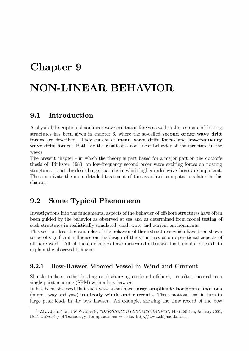
Chapter 9
NON-LINEAR BEHAVIOR
9.1 Introduction
A physical description of nonlinear wave excitation forces as well as the response of ‡oatingstructures has been given in chapter 6, where the so-called second order wave driftforces are described. They consist of mean wave drift forces and low-frequencywave drift forces. Both are the result of a non-linear behavior of the structure in thewaves.The present chapter - in which the theory is part based for a major part on the doctor’sthesis of [Pinkster, 1980] on low-frequency second order wave exciting forces on ‡oatingstructures - starts by describing situations in which higher order wave forces are important.These motivate the more detailed treatment of the associated computations later in thischapter.
9.2 Some Typical Phenomena
Investigations into the fundamental aspects of the behavior of o¤shore structures have oftenbeen guided by the behavior as observed at sea and as determined from model testing ofsuch structures in realistically simulated wind, wave and current environments.This section describes examples of the behavior of these structures which have been shownto be of signi…cant in‡uence on the design of the structures or on operational aspects ofo¤shore work. All of these examples have motivated extensive fundamental research toexplain the observed behavior.
9.2.1 Bow-Hawser Moored Vessel in Wind and Current
Shuttle tankers, either loading or discharging crude oil o¤shore, are often moored to asingle point mooring (SPM) with a bow hawser.It has been observed that such vessels can have large amplitude horizontal motions(surge, sway and yaw) in steady winds and currents. These motions lead in turn tolarge peak loads in the bow hawser. An example, showing the time record of the bow
0J.M.J. Journée and W.W. Massie, ”OFFSHORE HYDROMECHANICS”, First Edition, January 2001,Delft University of Technology. For updates see web site: http://www.shipmotions.nl.

9-2 CHAPTER 9. NON-LINEAR BEHAVIOR
hawser force of a 200 thousand ton deadweight (kTDW) tanker, is given in …gure 9.1. Thelower part of the …gure shows the bow hawser tension force as a function of time.
Figure 9.1: Unstable Horizontal Motions of a Bow Hawser Moored Tanker
This example shows that signi…cant dynamic e¤ects can occur, even in the absence oftime variations in the environmental forces. In this particular case, these e¤ects are dueto inherent instabilities in the horizontal motions of the tanker, which are related to thelength of the bow-hawser.Figure 9.2 shows the regions of unstable horizontal motions as a function of the anglebetween the wind and current on the one hand and the length of the bow-hawser on theother hand. See [Wichers, 1979] for further details.
9.2.2 Large Concrete Structure under Tow
After completion of a large concrete Gravity Base Structure in sheltered deep water, it istowed out to the …eld by 6 to 8 large ocean going tugs. Narrow and shallow fjord passageshave to be negotiated on the way out to the open sea. These passages put restrictions onthe swept path and the draft of the platform.Figure 9.3 shows that while under tow, this type of platform performs oscillatory motionsin all six degrees of freedom in addition to its constant forward motion. These oscillatorymotions are related - to a considerable extent - to the oscillatory components in the ‡owabout the platform, as well as the inherent ”towing stability” of the platform.Important aspects of the ‡ow about the platform are the vortex-shedding phenomenonabout the large diameter vertical columns and ‡ow separation about the large base struc-ture. The towing force needed for the transportation of the platform is important; thisdetermines the number and size of the tugs. The force necessary to hold the platform onlocation prior to being ballasted down to rest on the sea bed is determined by, among otherfactors, the current force that may be exerted by a tidal current. Figure …gure 9.4 showsan example of the quadratic increase of the current force with the current velocity.
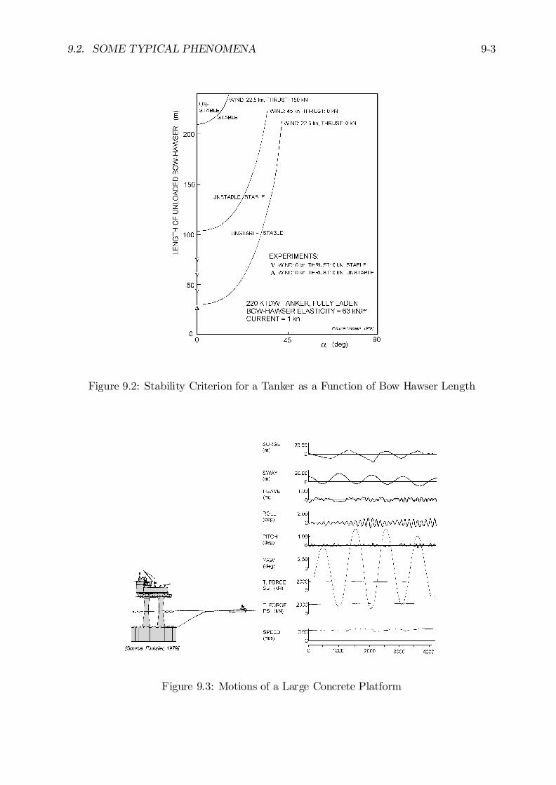
9.2. SOME TYPICAL PHENOMENA 9-3
Figure 9.2: Stability Criterion for a Tanker as a Function of Bow Hawser Length
Figure 9.3: Motions of a Large Concrete Platform
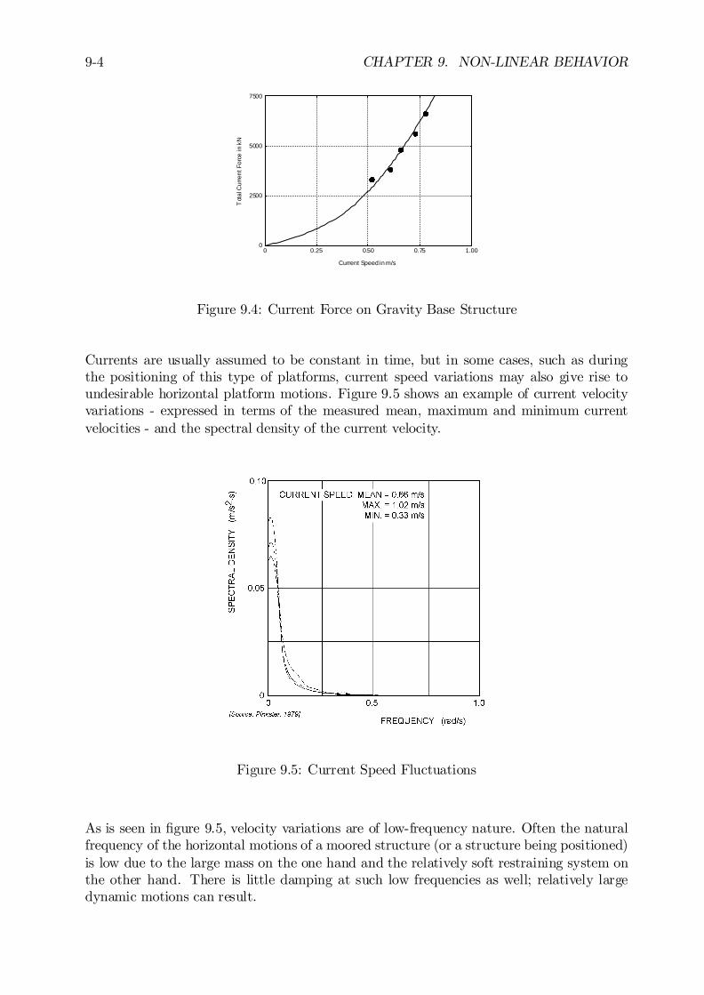
9-4 CHAPTER 9. NON-LINEAR BEHAVIOR
0
2500
5000
7500
0 0.25 0.50 0.75 1.00
Current Speed in m/s
Tot
al C
urre
nt F
orce
in k
N
Figure 9.4: Current Force on Gravity Base Structure
Currents are usually assumed to be constant in time, but in some cases, such as duringthe positioning of this type of platforms, current speed variations may also give rise toundesirable horizontal platform motions. Figure 9.5 shows an example of current velocityvariations - expressed in terms of the measured mean, maximum and minimum currentvelocities - and the spectral density of the current velocity.
Figure 9.5: Current Speed Fluctuations
As is seen in …gure 9.5, velocity variations are of low-frequency nature. Often the naturalfrequency of the horizontal motions of a moored structure (or a structure being positioned)is low due to the large mass on the one hand and the relatively soft restraining system onthe other hand. There is little damping at such low frequencies as well; relatively largedynamic motions can result.
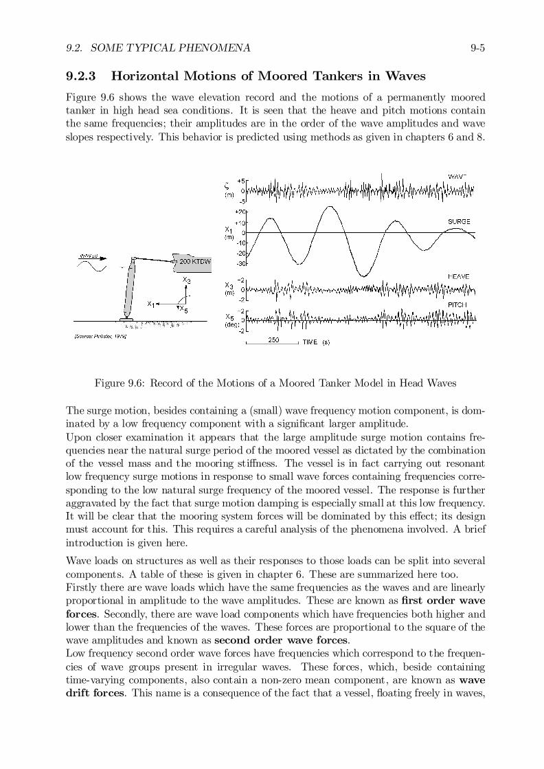
9.2. SOME TYPICAL PHENOMENA 9-5
9.2.3 Horizontal Motions of Moored Tankers in Waves
Figure 9.6 shows the wave elevation record and the motions of a permanently mooredtanker in high head sea conditions. It is seen that the heave and pitch motions containthe same frequencies; their amplitudes are in the order of the wave amplitudes and waveslopes respectively. This behavior is predicted using methods as given in chapters 6 and 8.
Figure 9.6: Record of the Motions of a Moored Tanker Model in Head Waves
The surge motion, besides containing a (small) wave frequency motion component, is dom-inated by a low frequency component with a signi…cant larger amplitude.Upon closer examination it appears that the large amplitude surge motion contains fre-quencies near the natural surge period of the moored vessel as dictated by the combinationof the vessel mass and the mooring sti¤ness. The vessel is in fact carrying out resonantlow frequency surge motions in response to small wave forces containing frequencies corre-sponding to the low natural surge frequency of the moored vessel. The response is furtheraggravated by the fact that surge motion damping is especially small at this low frequency.It will be clear that the mooring system forces will be dominated by this e¤ect; its designmust account for this. This requires a careful analysis of the phenomena involved. A briefintroduction is given here.
Wave loads on structures as well as their responses to those loads can be split into severalcomponents. A table of these is given in chapter 6. These are summarized here too.Firstly there are wave loads which have the same frequencies as the waves and are linearlyproportional in amplitude to the wave amplitudes. These are known as …rst order waveforces. Secondly, there are wave load components which have frequencies both higher andlower than the frequencies of the waves. These forces are proportional to the square of thewave amplitudes and known as second order wave forces.Low frequency second order wave forces have frequencies which correspond to the frequen-cies of wave groups present in irregular waves. These forces, which, beside containingtime-varying components, also contain a non-zero mean component, are known as wavedrift forces. This name is a consequence of the fact that a vessel, ‡oating freely in waves,
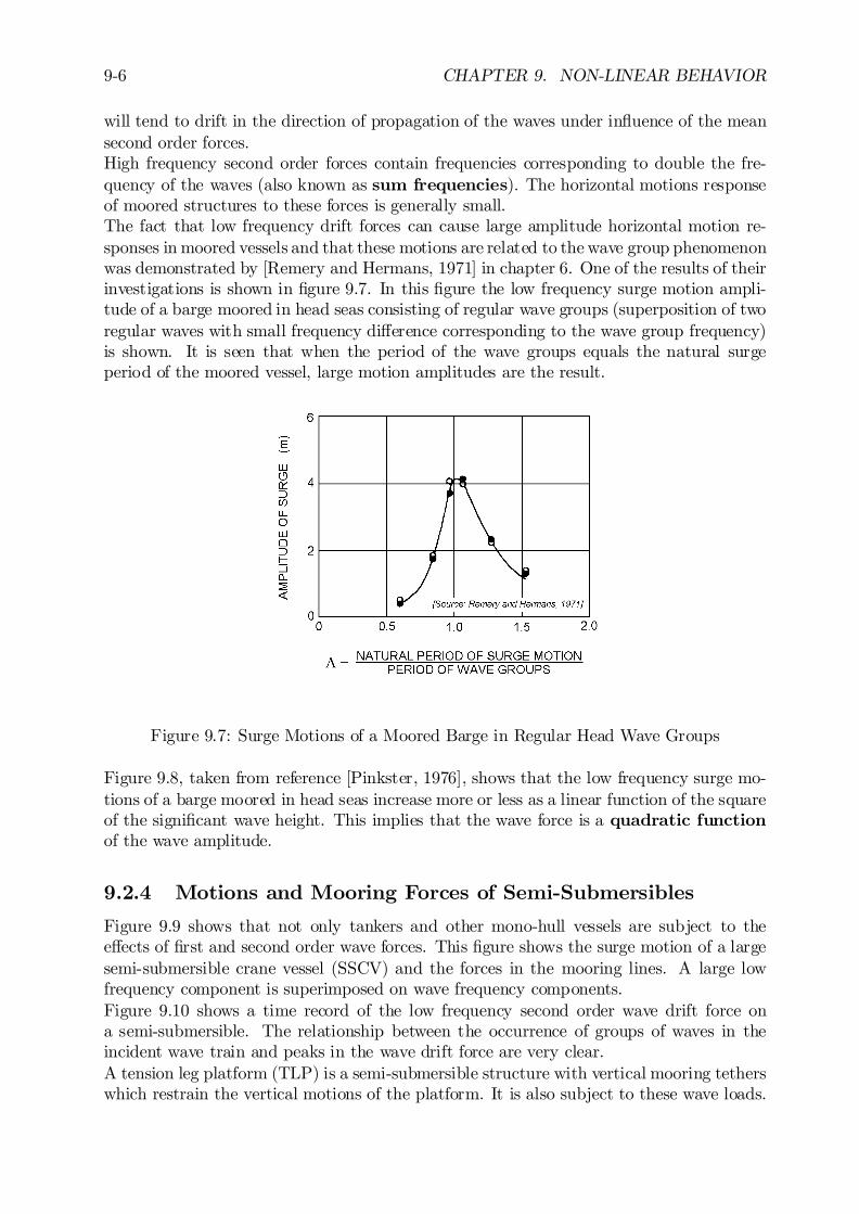
9-6 CHAPTER 9. NON-LINEAR BEHAVIOR
will tend to drift in the direction of propagation of the waves under in‡uence of the meansecond order forces.High frequency second order forces contain frequencies corresponding to double the fre-quency of the waves (also known as sum frequencies). The horizontal motions responseof moored structures to these forces is generally small.The fact that low frequency drift forces can cause large amplitude horizontal motion re-sponses in moored vessels and that these motions are related to the wave group phenomenonwas demonstrated by [Remery and Hermans, 1971] in chapter 6. One of the results of theirinvestigations is shown in …gure 9.7. In this …gure the low frequency surge motion ampli-tude of a barge moored in head seas consisting of regular wave groups (superposition of tworegular waves with small frequency di¤erence corresponding to the wave group frequency)is shown. It is seen that when the period of the wave groups equals the natural surgeperiod of the moored vessel, large motion amplitudes are the result.
Figure 9.7: Surge Motions of a Moored Barge in Regular Head Wave Groups
Figure 9.8, taken from reference [Pinkster, 1976], shows that the low frequency surge mo-tions of a barge moored in head seas increase more or less as a linear function of the squareof the signi…cant wave height. This implies that the wave force is a quadratic functionof the wave amplitude.
9.2.4 Motions and Mooring Forces of Semi-Submersibles
Figure 9.9 shows that not only tankers and other mono-hull vessels are subject to thee¤ects of …rst and second order wave forces. This …gure shows the surge motion of a largesemi-submersible crane vessel (SSCV) and the forces in the mooring lines. A large lowfrequency component is superimposed on wave frequency components.Figure 9.10 shows a time record of the low frequency second order wave drift force ona semi-submersible. The relationship between the occurrence of groups of waves in theincident wave train and peaks in the wave drift force are very clear.A tension leg platform (TLP) is a semi-submersible structure with vertical mooring tetherswhich restrain the vertical motions of the platform. It is also subject to these wave loads.
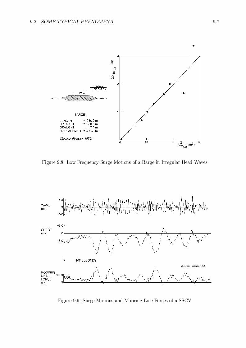
9.2. SOME TYPICAL PHENOMENA 9-7
Figure 9.8: Low Frequency Surge Motions of a Barge in Irregular Head Waves
Figure 9.9: Surge Motions and Mooring Line Forces of a SSCV
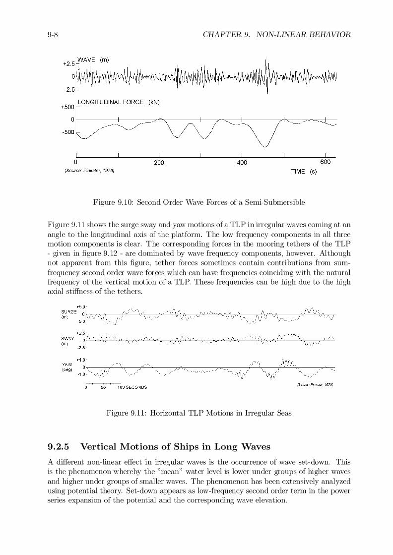
9-8 CHAPTER 9. NON-LINEAR BEHAVIOR
Figure 9.10: Second Order Wave Forces of a Semi-Submersible
Figure 9.11 shows the surge sway and yaw motions of a TLP in irregular waves coming at anangle to the longitudinal axis of the platform. The low frequency components in all threemotion components is clear. The corresponding forces in the mooring tethers of the TLP- given in …gure 9.12 - are dominated by wave frequency components, however. Althoughnot apparent from this …gure, tether forces sometimes contain contributions from sum-frequency second order wave forces which can have frequencies coinciding with the naturalfrequency of the vertical motion of a TLP. These frequencies can be high due to the highaxial sti¤ness of the tethers.
Figure 9.11: Horizontal TLP Motions in Irregular Seas
9.2.5 Vertical Motions of Ships in Long Waves
A di¤erent non-linear e¤ect in irregular waves is the occurrence of wave set-down. Thisis the phenomenon whereby the ”mean” water level is lower under groups of higher wavesand higher under groups of smaller waves. The phenomenon has been extensively analyzedusing potential theory. Set-down appears as low-frequency second order term in the powerseries expansion of the potential and the corresponding wave elevation.
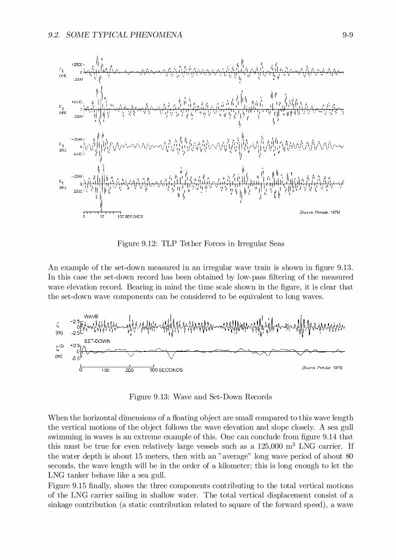
9.2. SOME TYPICAL PHENOMENA 9-9
Figure 9.12: TLP Tether Forces in Irregular Seas
An example of the set-down measured in an irregular wave train is shown in …gure 9.13.In this case the set-down record has been obtained by low-pass …ltering of the measuredwave elevation record. Bearing in mind the time scale shown in the …gure, it is clear thatthe set-down wave components can be considered to be equivalent to long waves.
Figure 9.13: Wave and Set-Down Records
When the horizontal dimensions of a ‡oating object are small compared to this wave lengththe vertical motions of the object follows the wave elevation and slope closely. A sea gullswimming in waves is an extreme example of this. One can conclude from …gure 9.14 thatthis must be true for even relatively large vessels such as a 125,000 m3 LNG carrier. Ifthe water depth is about 15 meters, then with an ”average” long wave period of about 80seconds, the wave length will be in the order of a kilometer; this is long enough to let theLNG tanker behave like a sea gull.Figure 9.15 …nally, shows the three components contributing to the total vertical motionsof the LNG carrier sailing in shallow water. The total vertical displacement consist of asinkage contribution (a static contribution related to square of the forward speed), a wave
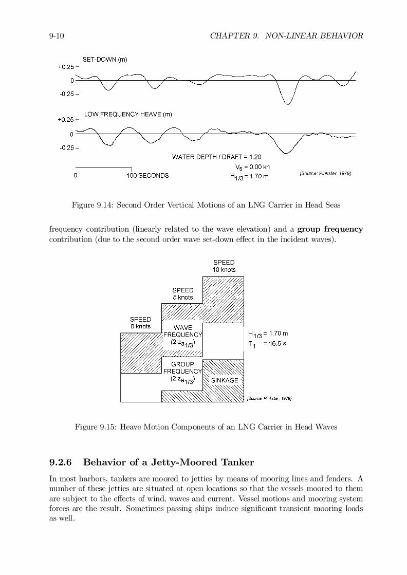
9-10 CHAPTER 9. NON-LINEAR BEHAVIOR
Figure 9.14: Second Order Vertical Motions of an LNG Carrier in Head Seas
frequency contribution (linearly related to the wave elevation) and a group frequencycontribution (due to the second order wave set-down e¤ect in the incident waves).
Figure 9.15: Heave Motion Components of an LNG Carrier in Head Waves
9.2.6 Behavior of a Jetty-Moored Tanker
In most harbors, tankers are moored to jetties by means of mooring lines and fenders. Anumber of these jetties are situated at open locations so that the vessels moored to themare subject to the e¤ects of wind, waves and current. Vessel motions and mooring systemforces are the result. Sometimes passing ships induce signi…cant transient mooring loadsas well.
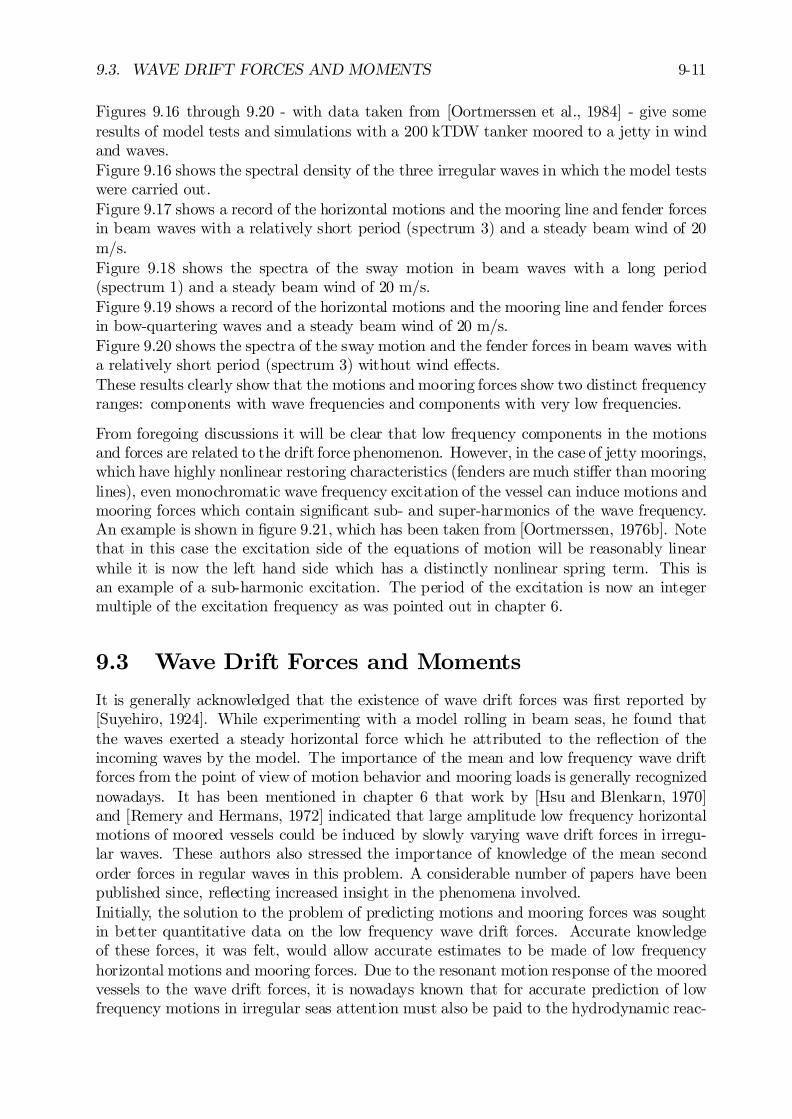
9.3. WAVE DRIFT FORCES AND MOMENTS 9-11
Figures 9.16 through 9.20 - with data taken from [Oortmerssen et al., 1984] - give someresults of model tests and simulations with a 200 kTDW tanker moored to a jetty in windand waves.Figure 9.16 shows the spectral density of the three irregular waves in which the model testswere carried out.Figure 9.17 shows a record of the horizontal motions and the mooring line and fender forcesin beam waves with a relatively short period (spectrum 3) and a steady beam wind of 20m/s.Figure 9.18 shows the spectra of the sway motion in beam waves with a long period(spectrum 1) and a steady beam wind of 20 m/s.Figure 9.19 shows a record of the horizontal motions and the mooring line and fender forcesin bow-quartering waves and a steady beam wind of 20 m/s.Figure 9.20 shows the spectra of the sway motion and the fender forces in beam waves witha relatively short period (spectrum 3) without wind e¤ects.These results clearly show that the motions and mooring forces show two distinct frequencyranges: components with wave frequencies and components with very low frequencies.
From foregoing discussions it will be clear that low frequency components in the motionsand forces are related to the drift force phenomenon. However, in the case of jetty moorings,which have highly nonlinear restoring characteristics (fenders are much sti¤er than mooringlines), even monochromatic wave frequency excitation of the vessel can induce motions andmooring forces which contain signi…cant sub- and super-harmonics of the wave frequency.An example is shown in …gure 9.21, which has been taken from [Oortmerssen, 1976b]. Notethat in this case the excitation side of the equations of motion will be reasonably linearwhile it is now the left hand side which has a distinctly nonlinear spring term. This isan example of a sub-harmonic excitation. The period of the excitation is now an integermultiple of the excitation frequency as was pointed out in chapter 6.
9.3 Wave Drift Forces and Moments
It is generally acknowledged that the existence of wave drift forces was …rst reported by[Suyehiro, 1924]. While experimenting with a model rolling in beam seas, he found thatthe waves exerted a steady horizontal force which he attributed to the re‡ection of theincoming waves by the model. The importance of the mean and low frequency wave driftforces from the point of view of motion behavior and mooring loads is generally recognizednowadays. It has been mentioned in chapter 6 that work by [Hsu and Blenkarn, 1970]and [Remery and Hermans, 1972] indicated that large amplitude low frequency horizontalmotions of moored vessels could be induced by slowly varying wave drift forces in irregu-lar waves. These authors also stressed the importance of knowledge of the mean secondorder forces in regular waves in this problem. A considerable number of papers have beenpublished since, re‡ecting increased insight in the phenomena involved.Initially, the solution to the problem of predicting motions and mooring forces was soughtin better quantitative data on the low frequency wave drift forces. Accurate knowledgeof these forces, it was felt, would allow accurate estimates to be made of low frequencyhorizontal motions and mooring forces. Due to the resonant motion response of the mooredvessels to the wave drift forces, it is nowadays known that for accurate prediction of lowfrequency motions in irregular seas attention must also be paid to the hydrodynamic reac-

9-12 CHAPTER 9. NON-LINEAR BEHAVIOR
Figure 9.16: Wave Spectra Used for a Jetty Moored Tanker
Figure 9.17: Behavior in Beam Waves and Beam Wind
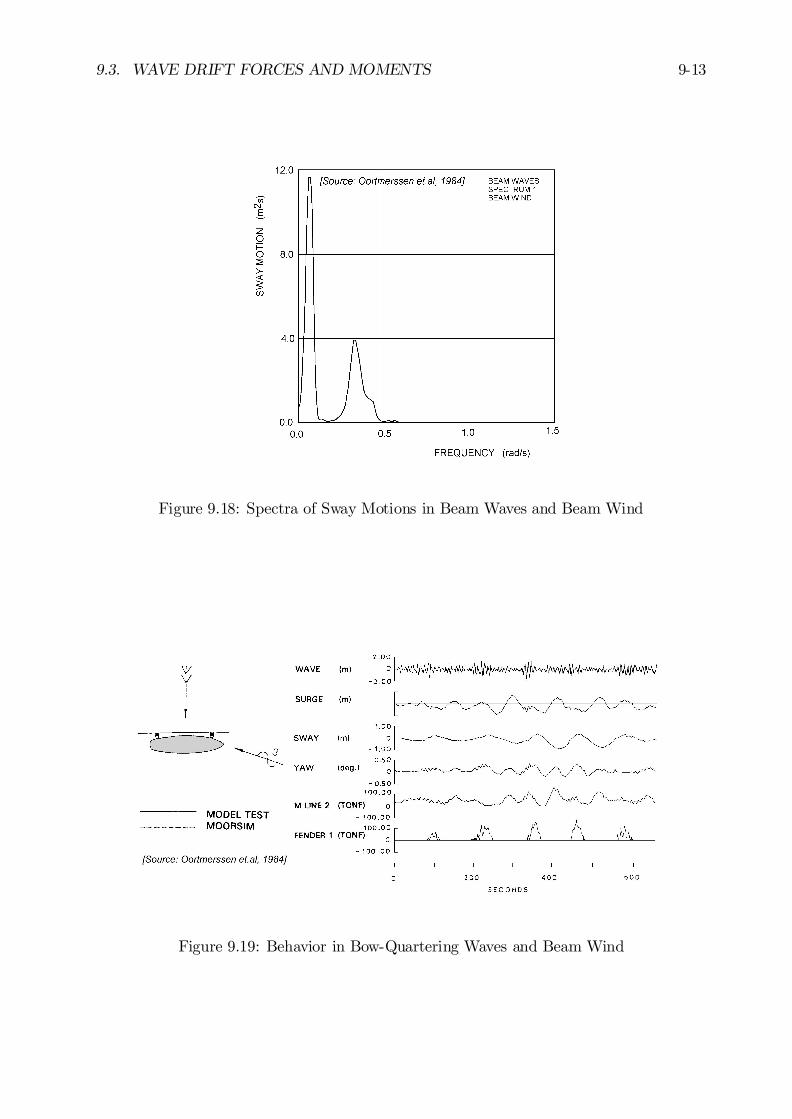
9.3. WAVE DRIFT FORCES AND MOMENTS 9-13
Figure 9.18: Spectra of Sway Motions in Beam Waves and Beam Wind
Figure 9.19: Behavior in Bow-Quartering Waves and Beam Wind
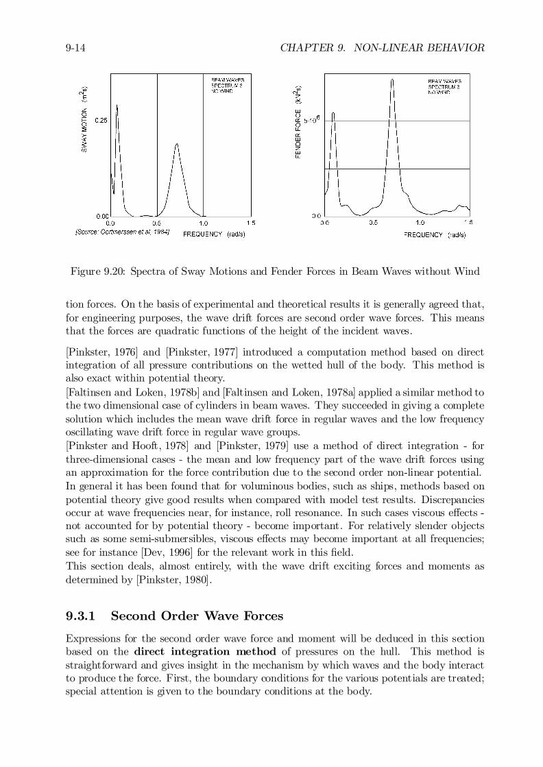
9-14 CHAPTER 9. NON-LINEAR BEHAVIOR
Figure 9.20: Spectra of Sway Motions and Fender Forces in Beam Waves without Wind
tion forces. On the basis of experimental and theoretical results it is generally agreed that,for engineering purposes, the wave drift forces are second order wave forces. This meansthat the forces are quadratic functions of the height of the incident waves.
[Pinkster, 1976] and [Pinkster, 1977] introduced a computation method based on directintegration of all pressure contributions on the wetted hull of the body. This method isalso exact within potential theory.[Faltinsen and Loken, 1978b] and [Faltinsen and Loken, 1978a] applied a similar method tothe two dimensional case of cylinders in beam waves. They succeeded in giving a completesolution which includes the mean wave drift force in regular waves and the low frequencyoscillating wave drift force in regular wave groups.[Pinkster and Hooft, 1978] and [Pinkster, 1979] use a method of direct integration - forthree-dimensional cases - the mean and low frequency part of the wave drift forces usingan approximation for the force contribution due to the second order non-linear potential.In general it has been found that for voluminous bodies, such as ships, methods based onpotential theory give good results when compared with model test results. Discrepanciesoccur at wave frequencies near, for instance, roll resonance. In such cases viscous e¤ects -not accounted for by potential theory - become important. For relatively slender objectssuch as some semi-submersibles, viscous e¤ects may become important at all frequencies;see for instance [Dev, 1996] for the relevant work in this …eld.This section deals, almost entirely, with the wave drift exciting forces and moments asdetermined by [Pinkster, 1980].
9.3.1 Second Order Wave Forces
Expressions for the second order wave force and moment will be deduced in this sectionbased on the direct integration method of pressures on the hull. This method isstraightforward and gives insight in the mechanism by which waves and the body interactto produce the force. First, the boundary conditions for the various potentials are treated;special attention is given to the boundary conditions at the body.
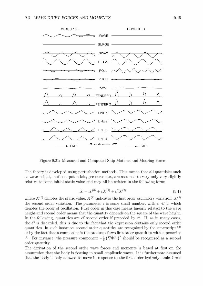
9.3. WAVE DRIFT FORCES AND MOMENTS 9-15
Figure 9.21: Measured and Computed Ship Motions and Mooring Forces
The theory is developed using perturbation methods. This means that all quantities suchas wave height, motions, potentials, pressures etc., are assumed to vary only very slightlyrelative to some initial static value and may all be written in the following form:
X =X(0) + "X(1) + "2X(2) (9.1)
whereX(0) denotes the static value, X(1) indicates the …rst order oscillatory variation, X(2)
the second order variation. The parameter " is some small number, with " ¿ 1, whichdenotes the order of oscillation. First order in this case means linearly related to the waveheight and second order means that the quantity depends on the square of the wave height.In the following, quantities are of second order if preceded by "2. If, as in many cases,the "2 is discarded, this is due to the fact that the expression contains only second orderquantities. In such instances second order quantities are recognized by the superscript (2)
or by the fact that a component is the product of two …rst order quantities with superscript(1). For instance, the pressure component ¡1
2
¡r©(1)
¢2should be recognized as a second
order quantity.The derivation of the second order wave forces and moments is based at …rst on theassumption that the body is ‡oating in small amplitude waves. It is furthermore assumedthat the body is only allowed to move in response to the …rst order hydrodynamic forces
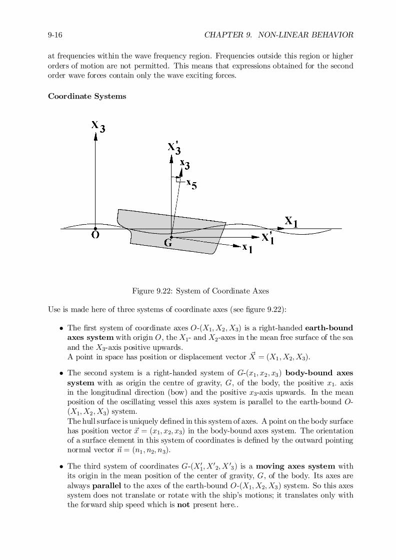
9-16 CHAPTER 9. NON-LINEAR BEHAVIOR
at frequencies within the wave frequency region. Frequencies outside this region or higherorders of motion are not permitted. This means that expressions obtained for the secondorder wave forces contain only the wave exciting forces.
Coordinate Systems
Figure 9.22: System of Coordinate Axes
Use is made here of three systems of coordinate axes (see …gure 9.22):
² The …rst system of coordinate axes O-(X1; X2; X3) is a right-handed earth-boundaxes system with origin O, theX1- and X2-axes in the mean free surface of the seaand the X3-axis positive upwards.A point in space has position or displacement vector ~X = (X1; X2; X3).
² The second system is a right-handed system of G-(x1; x2; x3) body-bound axessystem with as origin the centre of gravity, G, of the body, the positive x1- axisin the longitudinal direction (bow) and the positive x3-axis upwards. In the meanposition of the oscillating vessel this axes system is parallel to the earth-bound O-(X1; X2; X3) system.The hull surface is uniquely de…ned in this system of axes. A point on the body surfacehas position vector ~x = (x1; x2; x3) in the body-bound axes system. The orientationof a surface element in this system of coordinates is de…ned by the outward pointingnormal vector ~n = (n1; n2; n3).
² The third system of coordinates G-(X 01; X
02; X 0
3) is a moving axes system withits origin in the mean position of the center of gravity, G, of the body. Its axes arealways parallel to the axes of the earth-bound O-(X1; X2; X3) system. So this axessystem does not translate or rotate with the ship’s motions; it translates only withthe forward ship speed which is not present here..
9.3. WAVE DRIFT FORCES AND MOMENTS 9-17
The roll, pitch and yaw motions about the body-bound axes of the structure are given bythe Eulerian angles x4, x5 and x6, respectively.
First and Second Order Wave Loads
The …rst order wave loads have been de…ned in the chapter 7. There, the ”body-in-waves”has no motions (zero order) in the earth-bound axis system. The waves are approaching arestrained body. Thus, …rst order ‡uid motions and resulting …rst order ‡uid forces havebeen considered there.For the determination of the second order wave loads, the ”body-in-waves” is carrying outa …rst order harmonic motion, forced by …rst order wave loads. The waves are approachinga harmonic oscillating body. Then, second order ‡uid motions and resulting second order‡uid forces have to be considered too.
Body Motions
If the body has small amplitude motions resulting from the …rst order oscillatory waveforces, the resultant displacement vector ~X = (X1; X2; X3) of a point on the body - relativeto the earth-bound system of axes - is also a small …rst order quantity:
~X = " ~X(1) (9.2)
with:
~X(1) = ~XG(1)+ R(1) ¢ ~x (9.3)
where ~XG(1)
is the oscillatory …rst order motion vector of the center of gravity of the body,~x = (x1; x2;x3) is the position vector of the point on the body in the body-bound axessystem and R(1) is the linearized rotation transformation matrix, de…ned as:
R(1) =
264
0 ¡x(1)6 +x(1)5+x(1)6 0 ¡x(1)4¡x(1)5 +x(1)4 0
375 (9.4)
in which x(1)4 , x(1)5 and x(1)6 are the …rst order roll, pitch and yaw motions of the structure.Similarly, the velocity ~V of a point on the body relative to the earth-bound system of axes,O-(X1; X2; X3), is also a …rst order quantity and follows from:
~V = "~V (1) =!_X= "
!_X(1)
(9.5)
with:
!_X(1)
= ~V (1) =!_X(1)
G +:
R(1) ¢~x (9.6)
where:
:
R(1)=
264
0 ¡ :x(1)6 +
:x(1)5
+:x(1)6 0 ¡ :
x(1)4
¡ _x(1)5 + _x(1)4 0
375 (9.7)
9-18 CHAPTER 9. NON-LINEAR BEHAVIOR
in which:x(1)
4 ,:x(1)
5 and:x(1)
6 are the …rst order roll, pitch and yaw angular velocities of thestructure.Note that ~X and ~V and their derivatives are the (oscillatory) motions of the body; so farthey are not the motions of the ‡uid.The orientation of surface elements of the body relative to the G-(x1; x2; x3) body-boundaxes are denoted by the outward pointing normal vector ~n. When the body is carryingout small …rst order motions, the orientation of a surface element relative to the …xedO-(X1; X2; X3) or G-(X 0
1; X02; X
03) system of axes becomes:
~N = ~n + " ~N (1) (9.8)
with:
~N (1) = R(1) ¢ ~n (9.9)
where the linearized rotation transformation matrices, R(1), follows from equation 9.4.
Fluid Motions
The ‡uid domain is - just as when determining the hydromechanical coe¢cients in chapter7 - bounded by: 1) the surface of the body, 2) the free sea surface, 3) the sea bed and 4)a vertical cylinder with an in…nite radius. Assuming that the ‡uid is inviscid, irrotational,homogeneous and incompressible, the ‡uid motion may be described by means of thevelocity potential ©:
© = "©(1)+ "2©(2) + :::::: (9.10)
The potentials are de…ned relative to the earth-bound system of axes, O-(X1; X2; X3).As has been pointed out in chapter 7, the (linearized) …rst order potential ©(1) consists ofthe sum of potentials associated with the undisturbed incoming waves, ©(1)w , the di¤ractedwaves, ©(1)d , and waves due to the …rst order body motions, ©(1)b , respectively; thus:
©(1) = ©(1)w + ©(1)d +©(1)b (9.11)
Continuity Condition
Both the …rst and the second order potentials must satisfy the equation of continuity withinthe ‡uid domain; the Laplace equation (see chapter 7) has to be ful…lled by both potentialsas well:
r2©(1) = 0 and r2©(2) = 0 (9.12)
Sea Bed Boundary Condition
Both potentials must satisfy the boundary condition at the horizontal sea bed, too:
@©(1)
@X3= 0 and
@©(2)
@X3= 0 for: X3 = ¡h (9.13)
where h is the water depth in the O-(X1; X2; X3) axis system.

9.3. WAVE DRIFT FORCES AND MOMENTS 9-19
Free Surface Boundary Condition
In order to derive the boundary condition at the mean free surface use has to be made ofthe Bernoulli equation and the assumption that ‡uid elements in the free surface remainthere at all times (no-leak condition); see chapter 7. A Taylor expansion can be usedto transform the boundary conditions at the actual moving free surface (X3 = ³) intoboundary conditions at the mean free surface (X3 = 0); see also chapter 5.Then the homogeneous boundary condition becomes:
g ¢ @©(1)
@X3+@2©(1)
@t2= 0 (9.14)
For the particular solution of the boundary condition of ©(2), only the …nal result -which is very complex to solve as will be explained later - is given here:
g ¢ @©(2)
@X3+@2©(2)
@t2= ¡2
µ~r©(1) ¢ ~r@©
(1)
@t
¶+@©(1)
@t¢µ@2©(1)
@X23
+1
g¢ @
2
@t2
µ@©(1)
@X3
¶¶
(9.15)
This equation will be used further on in this chapter.
Body Boundary Condition
In general the boundary condition on the body is that no ‡uid passes through the hull(no-leak condition); the relative velocity between the ‡uid and the hull in the direction ofthe normal to the hull must be zero; see chapter 7.This boundary condition has to be satis…ed at the instantaneous position of the hullsurface; thus the ‡uid motions in the direction of the normal on the body, ~r© ¢ ~N , haveto be equal to the body motion in this normal direction, ~V ¢ ~N :
~r© ¢ ~N = ~V ¢ ~N (9.16)
or taking into account equations 9.5, 9.8 and 9.10:³"~r©(1) + "2~r©(2)
´¢³~n + " ~N (1)
´=
³"~V (1)
´¢³~n + " ~N (1)
´(9.17)
Grouping similar powers of " results in the …rst and second order body boundary conditions.The boundary conditions for the …rst order potential, "©(1), on the body is as follows:
~r©(1) ¢ ~n = ~V (1) ¢ ~n (9.18)
The boundary condition for the second order potential on the body, "2©(2), states that:
~r©(2) ¢ ~n =³~V (1) ¡ ~r©(1)
´¢ ~N (1) (9.19)
in which the …rst part, ~V (1) ¢ ~N (1), represents the body motions and the second part,~r©(1) ¢ ~N (1), the ‡uid motions.Equations 9.18 and 9.19 have to be satis…ed at the instantaneous position of the surfaceof the body. Assuming that the motions are small, and applying a Taylor expansion,
9-20 CHAPTER 9. NON-LINEAR BEHAVIOR
similar conditions may be stipulated for the potentials at the mean position of thehull surface.The …rst order boundary condition then becomes:
~r©(1) ¢ ~n = ~V (1) ¢ ~n (9.20)
and the second order boundary condition becomes:
~r©(2) ¢ ~n = ¡³~X(1) ¢ ~r
´¢³~r©(1) ¢ ~n
´+
³~V (1) ¡ ~r©(1)
´¢ ~N (1) (9.21)
in which the last term is the di¤erence of the two velocity vectors along the hull surfacecaused by the …rst order change of the direction normal.The potentials and their derivatives in equations 9.20 and 9.21 have to be evaluated at themean position of the body.
Substitution of equation 9.11 in boundary condition 9.20 - so splitting the potential inthree parts - yields the following:
³~r©(1)w + ~r©(1)d + ~r©(1)b
´¢ ~n = ~V (1) ¢ ~n (9.22)
It is customary to decompose this equation into two components:
² Di¤raction component:³~r©(1)w + ~r©(1)d
´¢ ~n = 0 (see chapter 7) (9.23)
or (9.24)~r©(1)d ¢ ~n = ¡~r©(1)w ¢ ~n (9.25)
² Motion component:~r©(1)b ¢ ~n = ~V (1) ¢ ~n (9.26)
The methods in use to solve for the unknown …rst order potentials ©(1)w , ©(1)d and ©(1)b havealready been discussed in chapters 5 and 7.
Substitution of the …rst order potential ©(1) from 9.11 in the non-homogeneous second orderfree surface boundary condition of equation 9.15 shows that the second order potentialincludes in the most general form the following components:
©(2) = ©(2)d (9.27)
+©(2)ww +©(2)dd + ©
(2)bb +©
(2)wd + ©
(2)wb + ©
(2)db + ©
(2)dw + ©
(2)bw +©
(2)bd
The …rst potential on the right-hand side of equation 9.27, ©(2)d , is a potential which satis…esthe homogeneous boundary condition:
g ¢ @©(2)d
@X3+@2©(2)d@t2
= 0 (9.28)
9.3. WAVE DRIFT FORCES AND MOMENTS 9-21
and ©(2)d is therefore an ”ordinary” potential which satis…es the linearized free surface
condition.
The last nine components on the right-hand side of equation 9.27 are potentials which areparticular solutions to the type of boundary condition as given in equation 9.18.For instance for ©(2)ww:
g ¢ @©(2)ww
@X3+@2©(2)ww@t2
= ¡2Ã~r©(1)w ¢ ~r@©
(1)w
@t
!+@©(1)w@t
Ã@2©(1)w@X2
3
+1
g¢ @
2
@t2
Ã@©(1)w@X3
!!(9.29)
Equation 9.27 can be written simpli…ed by letting ©(2)w represent the sum of the last ninecomponents on the right-hand side of the equation, so that:
©(2) = ©(2)d +©(2)w (9.30)
This ©(2)w may be regarded as the second order equivalent of the …rst order undisturbedincoming wave potential ©(1)w .Substitution of equation 9.30 in the second order boundary condition 9.21 yields:
³~r©(2)w + ~r©(2)d
´¢ ~n = ¡
³~X (1) ¢ ~r
´¢ ~r©(1) ¢ ~n +
³~V (1) ¡ ~r©(1)
´¢ ~N (1) (9.31)
or for the di¤raction potential:
~r©(2)d ¢ ~n = ¡~r©(2)w ¢ ~n ¡³~X(1) ¢ ~r
´¢~r©(1) ¢ ~n +
³~V (1) ¡ ~r©(1)
´¢ ~N (1) (9.32)
If the right-hand side of this equation is known, ©(2)d can be solved for the entire structureusing numerical methods.
In general, however, ©(2)w in equation 9.32 presents a problem due to the complexityof the surface boundary condition expressed by equation 9.15.[Faltinsen and Loken, 1978a] have found exact solutions of this problem for two-dimensionalcases, applicable to vessels in beam seas. [Newman, 1993] has developed numerical meth-ods to solve for the second order potential for the three-dimensional case. [Pinkster, 1980]suggest an approximation for ©(2)d which is applicable to three-dimensional problems.In a later section of this chapter it will be shown that the second order potential ©(2)daccounts only for a part of the second order wave forces.
Boundary Conditions at In…nity
A radiation condition for the potentials ©(1)w , ©(1)b and ©(2)d - which states that at a greatdistance from the body the waves associated with these potentials move outwards - mustbe satis…ed. This restriction imposes a uniqueness which would not otherwise be present.Since the components of©(2)w are particular solutions to the free surface boundary condition9.15 - which is de…ned over the complete free surface - a radiation condition need not beimposed on this term.

9-22 CHAPTER 9. NON-LINEAR BEHAVIOR
Symmetry Condition
The symmetry conditions, as discussed in chapter 5 and 7, are not taken into account here.The structure can have any arbitrary under water form.
Pressure at a Point within the Fluid
If the velocity potential © is known, the ‡uid pressure at a point is determined using the(non-linear) Bernoulli equation (see chapter 5):
p = ¡½gX3 ¡ ½@©@t
¡ 1
2½
³~r©
´2(9.33)
Assuming that this point is carrying out small - …rst order - wave frequency motions, ~X(1),about a mean position, ~X(0), and applying a Taylor expansion to the pressure in its meanposition, yields:
p = p(0) + "p(1)+ "2p(2) (9.34)
where:
² Hydrostatic pressure:p(0) = ¡½gX(0)
3 (9.35)
² First order pressure:
p(1) = ¡½gX(1)3 ¡ ½@©
(1)
@t(9.36)
² Second order pressure:
p(2) = ¡12½
³~r©(1)
´2¡ ½@
2©(2)
@t2¡ ½
µ~X(1) ¢ ~r@©
(1)
@t
¶(9.37)
The derivatives of the potentials in the above equations have to be evaluated at the meanposition of the point.It has been assumed that the point is moving within the ‡uid domain. The same ex-pression can be used to determine the pressure on a point on the hull of the body. Thismeans that derivatives of the potentials are taken at the mean position of the hull. Thisposition is actually alternately within and outside the actual ‡uid domain. This appearsto be permissible if the potential functions are su¢ciently ”smooth” at the boundaries; see[Joseph, 1973]. This is assumed to be satis…ed in this case.
Direct Pressure Integration
Since in general one is concerned with the slow wave drift force induced motions of bodies inthe horizontal plane, the wave drift force should be determined in the G-(x; y; z) coordinatesystem.The ‡uid force exerted on the body, relative to the G-(x; y; z) system of axes - which is thesystem with axes parallel to the axes of the earth-bound system, O-(X1; X2; X3) - followsfrom:
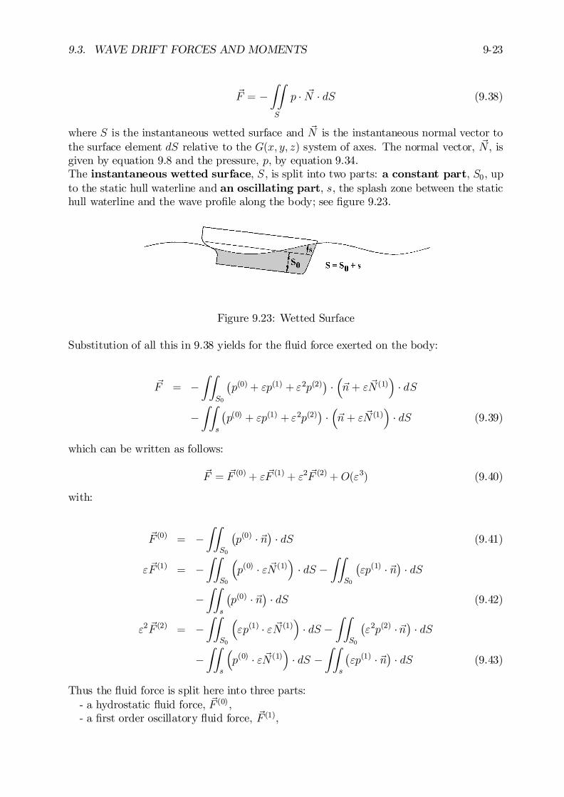
9.3. WAVE DRIFT FORCES AND MOMENTS 9-23
~F = ¡ZZ
S
p ¢ ~N ¢ dS (9.38)
where S is the instantaneous wetted surface and ~N is the instantaneous normal vector tothe surface element dS relative to the G(x; y; z) system of axes. The normal vector, ~N , isgiven by equation 9.8 and the pressure, p, by equation 9.34.The instantaneous wetted surface, S , is split into two parts: a constant part, S0, upto the static hull waterline and an oscillating part, s, the splash zone between the statichull waterline and the wave pro…le along the body; see …gure 9.23.
Figure 9.23: Wetted Surface
Substitution of all this in 9.38 yields for the ‡uid force exerted on the body:
~F = ¡ZZ
S0
¡p(0)+ "p(1) + "2p(2)
¢ ¢³~n + " ~N (1)
´¢ dS
¡ZZ
s
¡p(0) + "p(1) + "2p(2)
¢¢³~n + " ~N (1)
´¢ dS (9.39)
which can be written as follows:
~F = ~F (0)+ " ~F (1)+ "2 ~F (2)+ O("3) (9.40)
with:
~F (0) = ¡ZZ
S0
¡p(0) ¢ ~n
¢¢ dS (9.41)
" ~F (1) = ¡ZZ
S0
³p(0) ¢ " ~N (1)
´¢ dS ¡
ZZ
S0
¡"p(1) ¢ ~n
¢¢ dS
¡ZZ
s
¡p(0) ¢ ~n¢ ¢ dS (9.42)
"2 ~F (2) = ¡ZZ
S0
³"p(1) ¢ " ~N (1)
´¢ dS ¡
ZZ
S0
¡"2p(2) ¢ ~n
¢¢ dS
¡ZZ
s
³p(0) ¢ " ~N (1)
´¢ dS ¡
ZZ
s
¡"p(1) ¢ ~n
¢¢ dS (9.43)
Thus the ‡uid force is split here into three parts:- a hydrostatic ‡uid force, ~F (0) ,- a …rst order oscillatory ‡uid force, ~F (1),

9-24 CHAPTER 9. NON-LINEAR BEHAVIOR
- a second order ‡uid force, ~F (2):
The hydrostatic ‡uid force, ~F (0), follows from integration of the hydrostatic pressure,p(0), over the mean wetted surface, S0, as given in equation 9.41:
~F (0) = ¡ZZ
S0
¡p(0) ¢ ~n
¢¢ dS
= ½g
ZZ
S0
³X(0)3 ¢ ~n
´¢ dS
= (0; 0; ½gr) (9.44)
which yields only a vertical force contribution, F (0)3 , (no horizontal components):
F (0)3 = ½g
ZZ
S0
(X3 ¢ n3) ¢ dS
= ½gr (9.45)
in which r is here the volume of displacement.
The …rst order oscillatory ‡uid force, ~F (1), follows from equation 9.42:
~F (1) = ¡ZZ
S0
³p(0) ¢ ~N (1)
´¢ dS ¡
ZZ
S0
¡p(1) ¢ ~n
¢¢ dS
¡ZZ
s
¡p(0) ¢ ~n
¢¢ dS (9.46)
which includes three integral terms:
1. Products of the hydrostatic pressures, p(0), and the …rst order oscillatory componentsof the normal vector, ~N (1), which give …rst order force contributions over the constantpart, S0, of the wetted surface:
~F (1)A = ¡ZZ
S0
³p(0) ¢ ~N (1)
´¢ dS
= ½g
ZZ
S0
³X (0)3 ¢ ~N (1)
´¢ dS (9.47)
which is - after using equation 9.9 (linear rotation-transformation) - equal to:
~F (1)A = ½g
ZZ
S0
³X(0)3 ¢
©R(1) ¢ ~n
ª´¢ dS
= R(1) ¢ (0; 0; ½gr) (9.48)
This force component is caused by the rotating body axes; roll and pitch motionsresult in horizontal forces.
2. Products of the …rst order pressures, p(1), and the normal vector, ~n, which give also…rst order force contributions over the constant part, S0, of the wetted surface:
~F (1)B = ¡ZZ
S0
¡p(1) ¢ ~n
¢¢ dS (9.49)

9.3. WAVE DRIFT FORCES AND MOMENTS 9-25
3. Products of the hydrostatic pressures, p(0), and the normal vector, ~n, which give (inprinciple) …rst order force contributions because of its integration over the oscillatorypart, s, of the wetted surface.
~F (1)C = ¡ZZ
s
¡p(0) ¢ ~n
¢¢ dS = 0 (9.50)
This term is zero because the hydrostatic pressure at the oscillating surface, p(0), iszero because it has to be determined at X3 = 0.
Thus, the total …rst order ‡uid force follows from adding equations 9.48, 9.49 and 9.50:
~F (1) = R(1) ¢ (0; 0; ½gr)¡ZZ
S0
¡p(1) ¢ ~n
¢¢ dS (9.51)
The second order ‡uid force, ~F (2) , follows from equation 9.43:
~F (2) = ¡ZZ
S0
³p(1) ¢ ~N (1)
´¢ dS ¡
ZZ
S0
¡p(2) ¢ ~n
¢¢ dS
¡ZZ
s
³p(0) ¢ ~N (1)
´¢ dS ¡
ZZ
s
¡p(1) ¢ ~n
¢¢ dS (9.52)
which includes four integral terms:
1. Products of the …rst order pressures, p(1), and the …rst order oscillatory componentsof the normal vector, ~N (1), give second order force contributions over the constantpart, S0, of the wetted surface:
~F (2)A = ¡ZZ
S0
³p(1) ¢ ~N (1)
´¢ dS (9.53)
When using equation 9.9 for ~N (1) and equation 9.51 for the …rst order ‡uid force, onecan write:
~F (2)A = ¡R(1) ¢ZZ
S0
¡p(1) ¢ ~n
¢¢ dS
= R(1) ¢n~F (1) ¡R(1) ¢ (0; 0; ½gr)
o
= R(1) ¢n~F (1) ¡R(1) ¢ (0; 0;mg)
o(9.54)
Equation 9.54 shows that a second order force along the earth-bound axes followsfrom the rotation of the …rst order ‡uid force and the gravitational force acting onthe body; both relative to the body axes system. The last term deliver horizontalforces caused by the roll and pitch motions.According to Newton’s law, one may state that:
~F (1) ¡R(1) ¢ (0; 0; ½gr) = m¢!ÄX(1)
G (9.55)
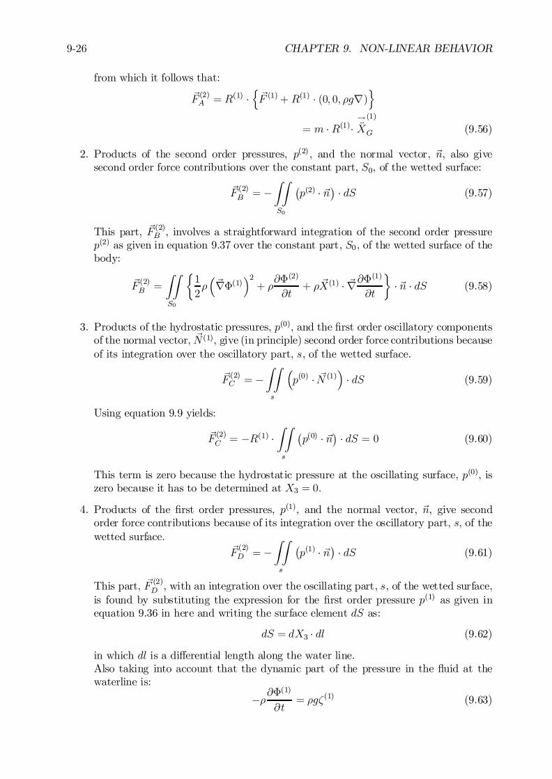
9-26 CHAPTER 9. NON-LINEAR BEHAVIOR
from which it follows that:
~F (2)A = R(1) ¢n~F (1)+ R(1) ¢ (0; 0; ½gr)
o
= m ¢R(1)¢!ÄX(1)
G (9.56)
2. Products of the second order pressures, p(2) , and the normal vector, ~n, also givesecond order force contributions over the constant part, S0, of the wetted surface:
~F (2)B = ¡ZZ
S0
¡p(2) ¢ ~n¢ ¢ dS (9.57)
This part, ~F (2)B , involves a straightforward integration of the second order pressurep(2) as given in equation 9.37 over the constant part, S0, of the wetted surface of thebody:
~F (2)B =
ZZ
S0
½1
2½³~r©(1)
´2+ ½
@©(2)
@t+ ½ ~X(1) ¢ ~r@©
(1)
@t
¾¢ ~n ¢ dS (9.58)
3. Products of the hydrostatic pressures, p(0), and the …rst order oscillatory componentsof the normal vector, ~N (1), give (in principle) second order force contributions becauseof its integration over the oscillatory part, s, of the wetted surface.
~F (2)C = ¡ZZ
s
³p(0) ¢ ~N (1)
´¢ dS (9.59)
Using equation 9.9 yields:
~F (2)C = ¡R(1) ¢ZZ
s
¡p(0) ¢ ~n¢ ¢ dS = 0 (9.60)
This term is zero because the hydrostatic pressure at the oscillating surface, p(0), iszero because it has to be determined at X3 = 0.
4. Products of the …rst order pressures, p(1), and the normal vector, ~n, give secondorder force contributions because of its integration over the oscillatory part, s, of thewetted surface.
~F(2)D = ¡
ZZ
s
¡p(1) ¢ ~n
¢¢ dS (9.61)
This part, ~F (2)D , with an integration over the oscillating part, s, of the wetted surface,is found by substituting the expression for the …rst order pressure p(1) as given inequation 9.36 in here and writing the surface element dS as:
dS = dX3 ¢ dl (9.62)
in which dl is a di¤erential length along the water line.Also taking into account that the dynamic part of the pressure in the ‡uid at thewaterline is:
¡½@©(1)
@t= ½g³(1) (9.63)
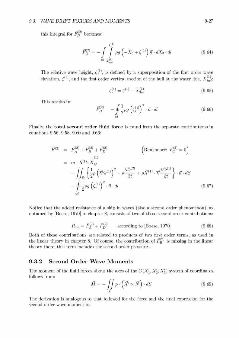
9.3. WAVE DRIFT FORCES AND MOMENTS 9-27
this integral for ~F (2)D becomes:
~F (2)D = ¡Z
wl
³(1)Z
X(1)3wl
½g³¡X3 + ³(1)
´~n ¢ dX3 ¢ dl (9.64)
The relative wave height, ³(1)r , is de…ned by a superposition of the …rst order waveelevation, ³(1), and the …rst order vertical motion of the hull at the water line, X(1)
3wl:
³(1)r = ³(1) ¡X (1)3wl (9.65)
This results in:~F(2)D = ¡
I
wl
1
2½g
³³(1)r
´2¢ ~n ¢ dl (9.66)
Finally, the total second order ‡uid force is found from the separate contributions inequations 9.56, 9.58, 9.60 and 9.66:
~F (2) = ~F (2)A + ~F (2)B + ~F (2)D
³Remember: ~F (2)C = 0
´
= m ¢R(1)¢!ÄX(1)
G
+
ZZ
S0
½1
2½
³~r©(1)
´2+ ½
@©(2)
@t+ ½ ~X(1) ¢ ~r@©
(1)
@t
¾¢ ~n ¢ dS
¡I
wl
1
2½g
³³(1)r
´2¢ ~n ¢ dl (9.67)
Notice that the added resistance of a ship in waves (also a second order phenomenon), asobtained by [Boese, 1970] in chapter 8, consists of two of these second order contributions:
Raw = ~F (2)A + ~F (2)D according to [Boese, 1970] (9.68)
Both of these contributions are related to products of two …rst order terms, as used inthe linear theory in chapter 8. Of course, the contribution of ~F (2)B is missing in the lineartheory there; this term includes the second order pressures.
9.3.2 Second Order Wave Moments
The moment of the ‡uid forces about the axes of the G(X 01; X
02; X
03) system of coordinates
follows from:~M = ¡
ZZ
S
p ¢³~X 0 £ ~N
´¢ dS (9.69)
The derivation is analogous to that followed for the force and the …nal expression for thesecond order wave moment is:
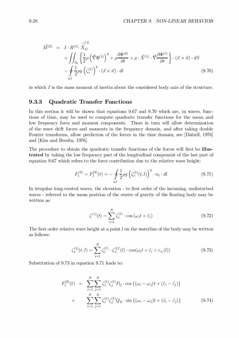
9-28 CHAPTER 9. NON-LINEAR BEHAVIOR
~M (2) = I ¢R(1)¢!ÄX(1)
G
+
ZZ
S0
½1
2½³~r©(1)
´2+ ½
@©(2)
@t+ ½ ¢ ~X(1) ¢ ~r@©
(1)
@t
¾¢ (~x £ ~n) ¢ dS
¡I
wl
1
2½g
³³(1)r
´2¢ (~x£ ~n) ¢ dl (9.70)
in which I is the mass moment of inertia about the considered body axis of the structure.
9.3.3 Quadratic Transfer Functions
In this section it will be shown that equations 9.67 and 9.70 which are, in waves, func-tions of time, may be used to compute quadratic transfer functions for the mean andlow frequency force and moment components. These in turn will allow determinationof the wave drift forces and moments in the frequency domain, and after taking doubleFourier transforms, allow prediction of the forces in the time domain, see [Dalzell, 1976]and [Kim and Breslin, 1976].
The procedure to obtain the quadratic transfer functions of the forces will …rst be illus-trated by taking the low frequency part of the longitudinal component of the last part ofequation 9.67 which refers to the force contribution due to the relative wave height:
F (2)1 = F (2)1 (t) = ¡I
wl
1
2½g
³³(1)r (t; l)
´2¢ n1 ¢ dl (9.71)
In irregular long-crested waves, the elevation - to …rst order of the incoming, undisturbedwaves - referred to the mean position of the centre of gravity of the ‡oating body may bewritten as:
³(1)(t) =NX
i=1
³(1)i ¢ cos (! it+ ~"i) (9.72)
The …rst order relative wave height at a point l on the waterline of the body may be writtenas follows:
³(1)r (t; l) =NX
i=1
³(1)i ¢ ³ (1)0ri(l) ¢ cos(!it+ ~"i + "ri(l)) (9.73)
Substitution of 9.73 in equation 9.71 leads to:
F (2)1 (t) =NX
i=1
NX
j=1
³(1)i ³(1)j Pij ¢ cos f(!i ¡ !j)t+ (~"i ¡ ~"j)g
+NX
i=1
NX
j=1
³(1)i ³(1)j Qij ¢ sin f(!i ¡ !j)t+ (~"i ¡ ~"j)g (9.74)
9.3. WAVE DRIFT FORCES AND MOMENTS 9-29
The high frequency terms (sum frequency terms) have been disregarded in this equation.In equation 9.74 Pij and Qij are the components of the time independent quadratic transferfunction with:
Pij =
I
wl
1
4½g³(1)
0ri (l) ¢ ³(1)0rj (l) ¢ cos f"ri(l) ¡ "rj (l)g¢n1 ¢ dl (9.75)
Qij =
I
wl
1
4½g³(1)
0ri (l) ¢ ³(1)0rj (l) ¢ sinf"ri(l) ¡ "rj (l)g ¢ n1 ¢ dl (9.76)
Taking now the low frequency part of the square of the wave elevation given by equation9.72 results in:
³³(1)LF(t)
´2=
NX
i=1
NX
j=1
1
2³(1)i ³
(1)j ¢ cos f(!i ¡ !j)t+ (~"i ¡ ~"j)g (9.77)
Comparison with equation 9.74 shows that Pij and Qij are transfer functions which givethat part of the wave drift force which is in-phase and out-of-phase respectively with thelow frequency part of the square of the incident waves.It will be clear that similar developments can be made for other contributions to the wavedrift forces which are dependent on products of …rst order quantities.
Approximation for Second Order Potential Contribution
As mentioned in a previous section, the contribution to the drift forces due to the secondorder potential presents special problems due to the non-linear nature of the free-surfacecondition and the complexity of the body boundary conditions. This section discusses amethod to approximate the e¤ect of the second order potential.The approximation is based on the assumption that the major part of the low frequencysecond order force due to the second order potential is the wave exciting force componentdue to the contribution ©(2)ww of the undisturbed incoming waves to the second order poten-tial. This assumes that the …rst order di¤raction and body motion potentials ©(1)d and ©(1)bare small relative to the undisturbed wave potential ©(1)w . This means that the right-handside of the free surface boundary condition of equation 9.15 only involves terms associatedwith the …rst order velocity potential ©(1)w of the undisturbed incoming waves. The secondorder potential which satis…es this boundary condition and the boundary condition at thesea bed as well as the equation of continuity has been given by [Bowers, 1975].We now consider a regular wave group travelling in the positive X1-direction consisting oftwo regular waves with frequencies !i and !j with ! i > !j.The …rst order velocity potential associated with these waves is:
©(1)w = ¡NX
i=1
³(1)i g cosh ki (X3 ¡ h)
! i cosh ki h¢ sin(ki X1¡ ! i t+ ~"i) (9.78)
The low frequency component of the second order potential associated with these waves isas follows:
©(2)ww = ¡NX
i=1
NX
j=1
³(1)i ³(1)j ¢ Aij ¢ coshf(ki ¡ kj)(X3 ¡h)g
cosh(ki ¡ kj)h¢
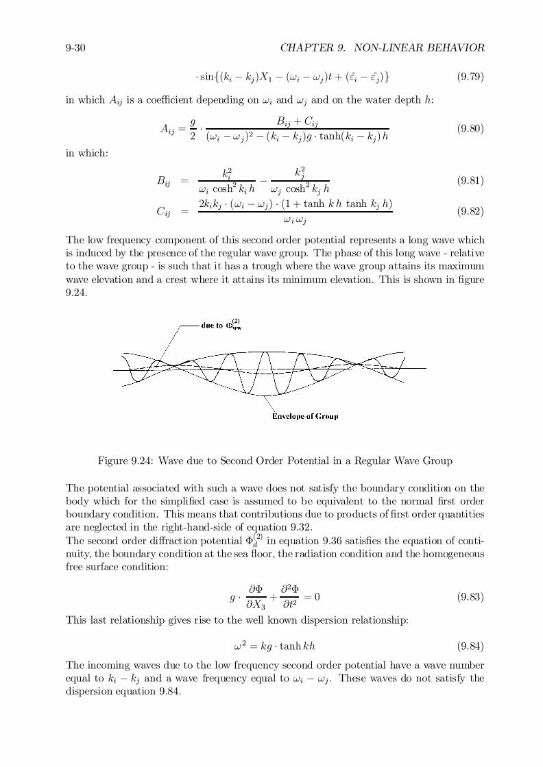
9-30 CHAPTER 9. NON-LINEAR BEHAVIOR
¢ sinf(ki ¡ kj)X1 ¡ (!i ¡ !j)t+ (~"i ¡ ~"j)g (9.79)
in which Aij is a coe¢cient depending on !i and !j and on the water depth h:
Aij =g
2¢ Bij + Cij(!i ¡!j)2 ¡ (ki ¡ kj)g ¢ tanh(ki ¡ kj)h
(9.80)
in which:
Bij =k2i
!i cosh2 ki h
¡ k2j!j cosh
2 kj h(9.81)
Cij =2kikj ¢ (!i ¡ !j) ¢ (1 + tanh k h tanh kj h)
! i !j(9.82)
The low frequency component of this second order potential represents a long wave whichis induced by the presence of the regular wave group. The phase of this long wave - relativeto the wave group - is such that it has a trough where the wave group attains its maximumwave elevation and a crest where it attains its minimum elevation. This is shown in …gure9.24.
Figure 9.24: Wave due to Second Order Potential in a Regular Wave Group
The potential associated with such a wave does not satisfy the boundary condition on thebody which for the simpli…ed case is assumed to be equivalent to the normal …rst orderboundary condition. This means that contributions due to products of …rst order quantitiesare neglected in the right-hand-side of equation 9.32.The second order di¤raction potential ©(2)d in equation 9.36 satis…es the equation of conti-nuity, the boundary condition at the sea ‡oor, the radiation condition and the homogeneousfree surface condition:
g ¢ @©@X3
+@2©
@t2= 0 (9.83)
This last relationship gives rise to the well known dispersion relationship:
!2 = kg ¢ tanhkh (9.84)
The incoming waves due to the low frequency second order potential have a wave numberequal to ki ¡ kj and a wave frequency equal to !i ¡ !j. These waves do not satisfy thedispersion equation 9.84.
9.3. WAVE DRIFT FORCES AND MOMENTS 9-31
If the incoming waves have a frequency of !i¡!j then the di¤racted waves have the samefrequency; the wave number will follow from the relationship:
(!i ¡ !j)2 = k g ¢ tanh k h (9.85)
In order to simplify the situation we allow the di¤racted waves to have the same wavenumber ki ¡ kj as the incoming waves. This means that di¤erences will occur in thedi¤racted waves further away from the body. Close to the body the situation will besimilar since the boundary condition at the body still has to be satis…ed. The reason forthis assumption regarding the wave number of the di¤racted waves will be apparent fromthe following.The problem has been reduced to a situation where one has to determine the wave excitingforce on the body due to a wave which has a velocity potential given by equation 9.79.The di¤racted waves have the same wave number as the incoming waves. This is solvedby considering the ordinary …rst order wave exciting force F (1) on the body in a regularwave with wave number equal to ki ¡ kj in an ordinary gravity …eld. For such a case theassociated wave frequency ! will be in accordance with the dispersion relationship equation9.84. The frequency of this wave can be made equal to the frequency !i¡!j of the secondorder waves by selecting a di¤erent value for the acceleration of gravity:
gij =(!i ¡ !j)2
(ki ¡ kj) ¢ tanh(ki ¡ kj)h(9.86)
Since the wave exciting force is proportional to the acceleration of gravity, the initial forceF (1) in a wave with frequency !, which follow from equation 9.84, becomes a second orderwave force with frequency !i ¡ !j by simply applying the factor:
nij =gijg
(9.87)
to the initial force.This does not complete the transformation however, since besides satisfying the require-ment that wave number and wave frequency be equal, the amplitude of the potentials mustalso be equal. After alteration of the acceleration of gravity, the transformed potential ofthe …rst order wave is:
© = ¡ ³(1)a gij(!i ¡ !j)
¢ coshf(ki ¡ kj)(X3 ¡ h)gcosh(ki ¡ kj) h
¢ sin f(ki ¡ kj)X1 ¡ (!i ¡ !j)t+ (~"i ¡ ~"j)g(9.88)
The amplitude of the second order potential is given in equation 9.79. Equality of theamplitudes means that:
³(1)a gij(!i ¡ !j)
= ³(1)i ³(1)j ¢ Aij (9.89)
This means that the …rst order wave amplitude must be selected so that:
³(1)a = ³(1)i ³(1)j ¢ Aij(!i ¡ !j)gij
(9.90)
The …rst order force F (1) is determined for a value of unity for the wave amplitude ³a. Sinceforces are proportional to the wave amplitude, equation 9.90 gives a second correction factor
9-32 CHAPTER 9. NON-LINEAR BEHAVIOR
which has to be applied to the force F (1) in order to give the required second order forceF (2):
F (2)ij = nij ¢ ³(1)i ³(1)j ¢ Aij (! i ¡ !j)
gij¢ F (1) (9.91)
which, taking into account equation 9.87, gives:
F (2)ij = fij ¢ F (1) (9.92)
where:
fij =³(1)i ³
(1)j ¢ Aij (!i ¡ !j)
g(9.93)
Equation 9.92 transforms a …rst order wave force into a second order wave force. As canbe seen from this equation, the second order force becomes a function of two frequencies!i and !j. This approximation for the second order force can also be expressed in termsof contributions to the coe¢cients Pij and Qij.
Wave Drift Forces in Regular Wave Groups
From the previous sections it was seen that the total wave drift forces may thus be expressedin terms of transfer functions which are a function of two frequencies.The most elementary sea state which gives low frequency wave drift forces is one whichconsists of two regular waves with amplitude, frequency and random phase of ³1; !1; "1 and³2; !2; "2 respectively, with !1 > !2.
³(t) = ³1 ¢ cos (!1t + "1) + ³2 ¢ cos (!2t+ "2) (9.94)
The wave drift force in such a case is:
F (2)(t) = ³21:P11 + ³22:P22
+³1³2(P12 + P21) ¢ cos f(!1 ¡ !2)t+ ("1 ¡ "2)g+³1³2(Q12 ¡Q21) ¢ sinf(!1¡ !2)t+ ("1 ¡ "2)g (9.95)
The frequency of the low frequency part of the wave drift force is equal to the di¤erencebetween the frequencies of the regular wave components. This is the frequency of theregular wave group which is the result of superposition of two regular waves (see …gure9.25). It is noted that the constant part of the wave drift force is the sum of the constantparts due to each of the wave components. The amplitude of the quadratic transfer functionis:
jTijj=qP 2ij + Q
2ij (9.96)
Since Pij andQij, etc. never occur in isolation, it can be so arranged that certain symmetryrelations are valid:
Pij = Pji (9.97)
Qij = ¡Qji (9.98)
jTijj = jTjij (9.99)
9.3. WAVE DRIFT FORCES AND MOMENTS 9-33
Figure 9.25: Regular Wave Group
Frequency Domain Calculation of Mean and Low Frequency Drift Force
The mean drift force in irregular waves with spectral density S³³(!) is found by putting!1 = !2 in equation 9.74:
F (2)1mean =NX
i=1
³(1)2
i ¢ Pii (9.100)
which, taking into account that:
³(1)2
i = 2 ¢ S³ (!i) ¢ d! i (see chapter 5) (9.101)
results in:
F (2)1mean = 2
1Z
0
S³(!) ¢ P (!; !) ¢ d! (9.102)
where P (!; !) is known as the mean drift force coe¢cient in regular waves.By using equation 9.74 with i = j, P (!; ! is also written as:
P (!; !) =F1³2a(!) (9.103)
Similarly it can be shown that the spectral density of the low frequency part of the wavedrift force is:
SF(¹) = 8
1Z
0
S³ (!1) ¢ S³(!2) ¢ jT(!1; !2)j2 ¢ d! (9.104)
where !1¡ !2 = ¹ is the low frequency and j T(!1; !2) j is the amplitude of the quadratictransfer function.Equation 9.104 can also be written as:
SF(¹) = 8
1Z
0
S³ (! +¹) ¢ S³(!) ¢ jT(! + ¹; !)j2 ¢ d! (9.105)
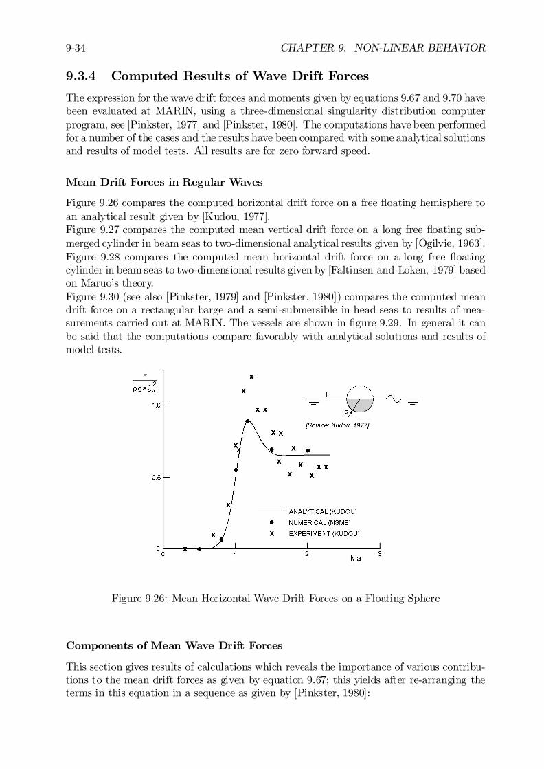
9-34 CHAPTER 9. NON-LINEAR BEHAVIOR
9.3.4 Computed Results of Wave Drift Forces
The expression for the wave drift forces and moments given by equations 9.67 and 9.70 havebeen evaluated at MARIN, using a three-dimensional singularity distribution computerprogram, see [Pinkster, 1977] and [Pinkster, 1980]. The computations have been performedfor a number of the cases and the results have been compared with some analytical solutionsand results of model tests. All results are for zero forward speed.
Mean Drift Forces in Regular Waves
Figure 9.26 compares the computed horizontal drift force on a free ‡oating hemisphere toan analytical result given by [Kudou, 1977].Figure 9.27 compares the computed mean vertical drift force on a long free ‡oating sub-merged cylinder in beam seas to two-dimensional analytical results given by [Ogilvie, 1963].Figure 9.28 compares the computed mean horizontal drift force on a long free ‡oatingcylinder in beam seas to two-dimensional results given by [Faltinsen and Loken, 1979] basedon Maruo’s theory.Figure 9.30 (see also [Pinkster, 1979] and [Pinkster, 1980]) compares the computed meandrift force on a rectangular barge and a semi-submersible in head seas to results of mea-surements carried out at MARIN. The vessels are shown in …gure 9.29. In general it canbe said that the computations compare favorably with analytical solutions and results ofmodel tests.
Figure 9.26: Mean Horizontal Wave Drift Forces on a Floating Sphere
Components of Mean Wave Drift Forces
This section gives results of calculations which reveals the importance of various contribu-tions to the mean drift forces as given by equation 9.67; this yields after re-arranging theterms in this equation in a sequence as given by [Pinkster, 1980]:
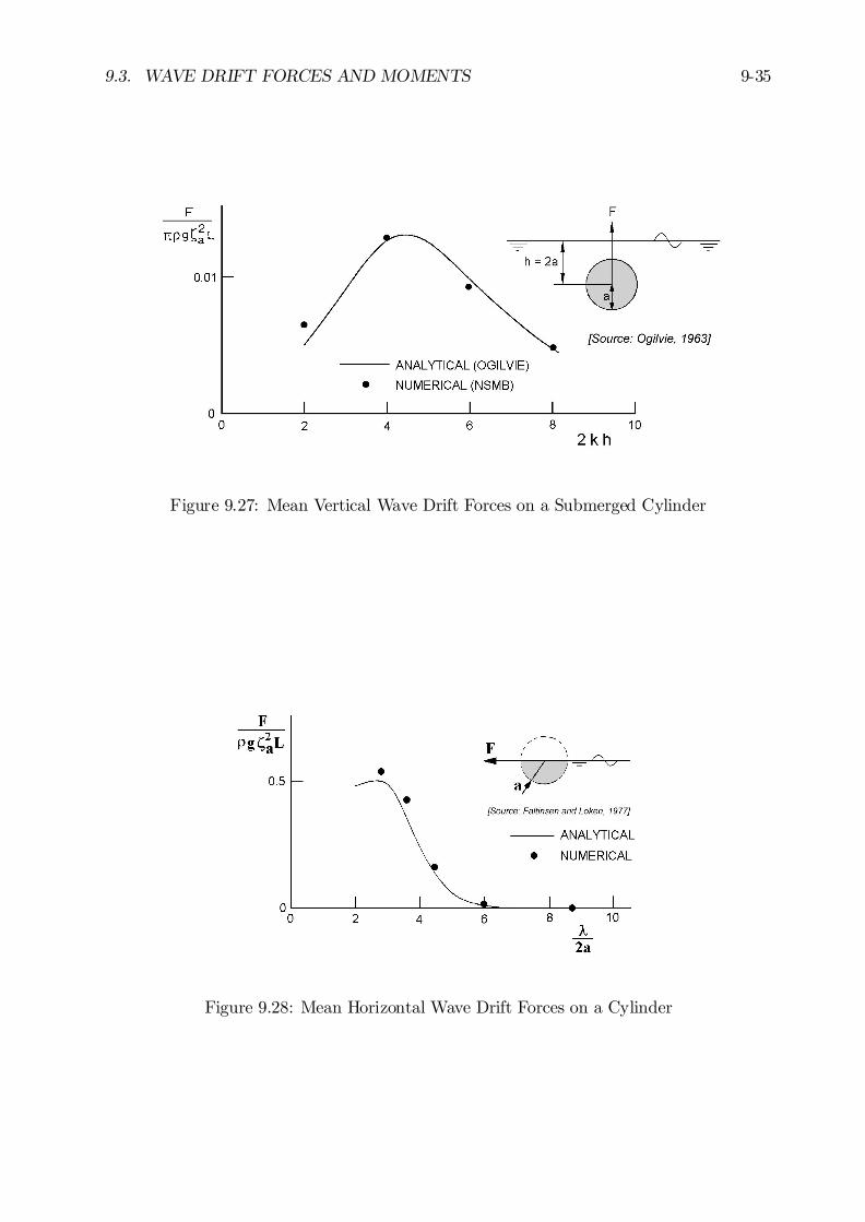
9.3. WAVE DRIFT FORCES AND MOMENTS 9-35
Figure 9.27: Mean Vertical Wave Drift Forces on a Submerged Cylinder
Figure 9.28: Mean Horizontal Wave Drift Forces on a Cylinder

9-36 CHAPTER 9. NON-LINEAR BEHAVIOR
Figure 9.29: Vessels used for Experiments
Figure 9.30: Mean Surge Drift Forces in Regular Head Waves
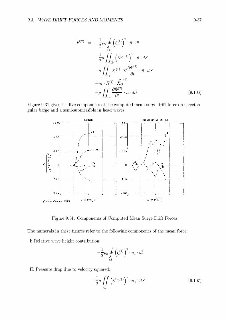
9.3. WAVE DRIFT FORCES AND MOMENTS 9-37
~F (2) = ¡12½g
I
wl
³³(1)r
´2¢ ~n ¢ dl
+1
2½
ZZ
S0
³~r©(1)
´2¢ ~n ¢ dS
+½
ZZ
S0
~X (1) ¢ ~r@©(1)
@t¢ ~n ¢ dS
+m ¢R(1) ¢ Ä~XG(1)
+½
ZZ
S0
@©(2)
@t¢ ~n ¢ dS (9.106)
Figure 9.31 gives the …ve components of the computed mean surge drift force on a rectan-gular barge and a semi-submersible in head waves.
Figure 9.31: Components of Computed Mean Surge Drift Forces
The numerals in these …gures refer to the following components of the mean force:
I: Relative wave height contribution:
¡12½g
I
wl
³³(1)r
´2¢ n1 ¢ dl
II: Pressure drop due to velocity squared:
1
2½
ZZ
S0
³~r©(1)
´2¢n1 ¢ dS (9.107)

9-38 CHAPTER 9. NON-LINEAR BEHAVIOR
III: Pressure due to product of gradient of …rst order pressure and …rst order motion:
½
ZZ
S0
³~X(1) ¢ ~r©(1)
´¢ n1 ¢ dS (9.108)
IV: Contribution due to product of pitch motion and heave inertia force:
m ¢ x(1)5 ¢ ÄX (1)3G (9.109)
V: Contribution due to the second order potential ©(2), which is zero in regular waves:
½
ZZ
S0
@©(2)
@t¢ ~n ¢ dS (9.110)
The results in …gure 9.31 show that in general contribution I due to the relative wave heightis dominant, while the three remaining terms II, III and IV tend only to reduce somewhatthe e¤ect of contribution I. For high frequencies (to the right in the …gures) terms III andIV vanish since the body motions - on which these terms are dependent - reduce to zeroin short waves. This leaves only the terms I and II.For the semi-submersible in …gure 9.31 it is apparent that it is the wave drift forces actingon the columns which form the greater part of the total horizontal wave drift forces.Figure 9.32 shows the computed contributions to the mean horizontal drift force on the‡oating sphere. In this case only contributions I, II and III play a part. As the frequencyincreases again only contributions I and II remain.Figure 9.33 shows the computed contributions to the vertical force on the submergedcylinder in beam seas. Since there is no waterline, only contributions II and III play a role.For high frequencies only II remains.
9.3.5 Low Frequency Motions
In view of the analogy which exists between the low frequency waves, the drift forces andthe low frequency part of the square of the elevations of the incident waves as indicatedby equations 9.74 and 9.77, we will look at some aspects of the waves. This will give someindications regarding the properties of the low frequency wave drift forces.The irregular waves are assumed to behave as a random Gaussian process. Thus, the waveelevation in a …xed point in irregular waves, may be written as follows:
³(t) =NX
i=1
³i ¢ sin (!it + ~"i) (9.111)
where ~"i is a random phase angle.In amplitude modulated form this becomes:
³(t) = A(t) ¢ sin (!0t+ "(t)) (9.112)
where:
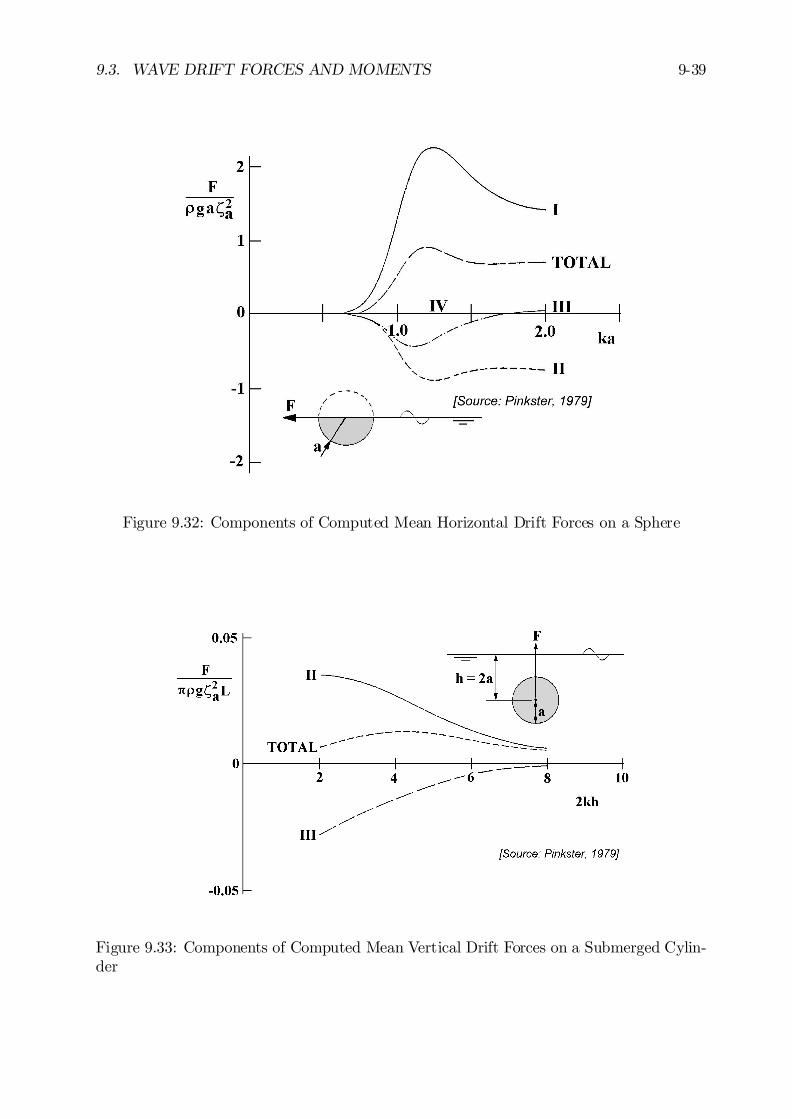
9.3. WAVE DRIFT FORCES AND MOMENTS 9-39
Figure 9.32: Components of Computed Mean Horizontal Drift Forces on a Sphere
Figure 9.33: Components of Computed Mean Vertical Drift Forces on a Submerged Cylin-der
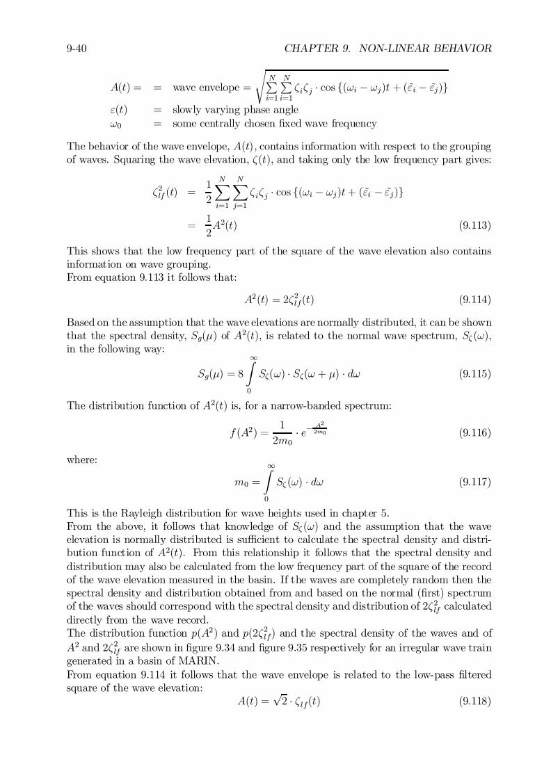
9-40 CHAPTER 9. NON-LINEAR BEHAVIOR
A(t) = = wave envelope =
sNPi=1
NPi=1
³i³j ¢ cos f(!i ¡ !j)t + (~"i ¡ ~"j)g
"(t) = slowly varying phase angle!0 = some centrally chosen …xed wave frequency
The behavior of the wave envelope, A(t), contains information with respect to the groupingof waves. Squaring the wave elevation, ³(t), and taking only the low frequency part gives:
³2lf (t) =1
2
NX
i=1
NX
j=1
³i³j ¢ cos f(!i ¡ !j)t+ (~"i ¡ ~"j)g
=1
2A2(t) (9.113)
This shows that the low frequency part of the square of the wave elevation also containsinformation on wave grouping.From equation 9.113 it follows that:
A2(t) = 2³2lf(t) (9.114)
Based on the assumption that the wave elevations are normally distributed, it can be shownthat the spectral density, Sg(¹) of A2(t), is related to the normal wave spectrum, S³ (!),in the following way:
Sg(¹) = 8
1Z
0
S³(!) ¢ S³(! + ¹) ¢ d! (9.115)
The distribution function of A2(t) is, for a narrow-banded spectrum:
f (A2) =1
2m0¢ e¡
A2
2m0 (9.116)
where:
m0 =
1Z
0
S³ (!) ¢ d! (9.117)
This is the Rayleigh distribution for wave heights used in chapter 5.From the above, it follows that knowledge of S³ (!) and the assumption that the waveelevation is normally distributed is su¢cient to calculate the spectral density and distri-bution function of A2(t). From this relationship it follows that the spectral density anddistribution may also be calculated from the low frequency part of the square of the recordof the wave elevation measured in the basin. If the waves are completely random then thespectral density and distribution obtained from and based on the normal (…rst) spectrumof the waves should correspond with the spectral density and distribution of 2³2lf calculateddirectly from the wave record.The distribution function p(A2) and p(2³2lf) and the spectral density of the waves and ofA2 and 2³2lf are shown in …gure 9.34 and …gure 9.35 respectively for an irregular wave traingenerated in a basin of MARIN.From equation 9.114 it follows that the wave envelope is related to the low-pass …lteredsquare of the wave elevation:
A(t) =p2 ¢ ³ lf(t) (9.118)
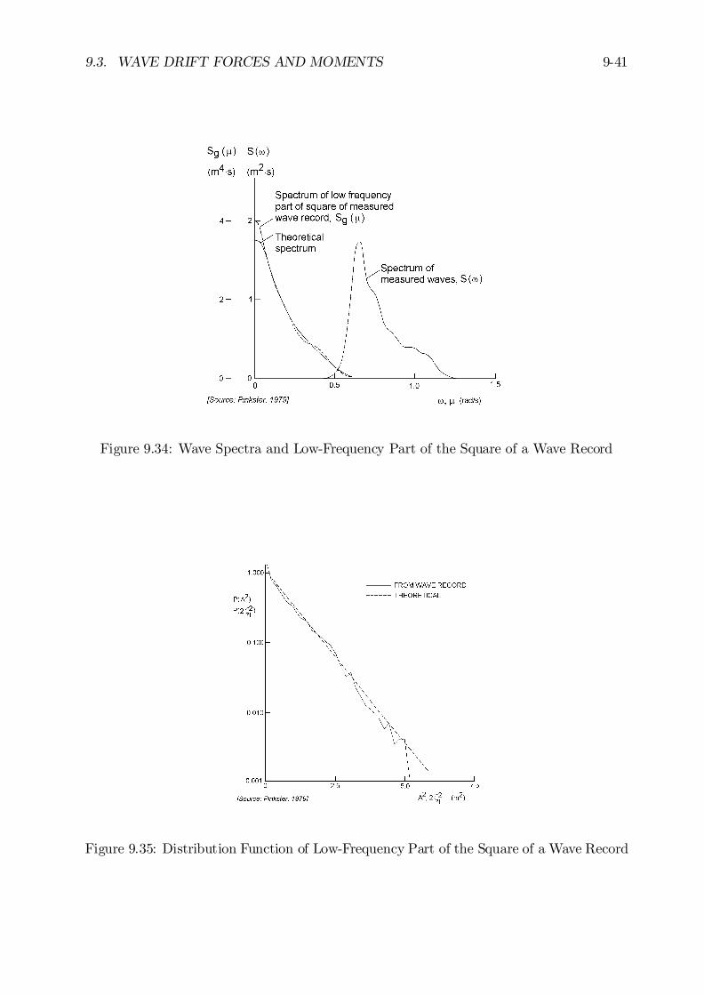
9.3. WAVE DRIFT FORCES AND MOMENTS 9-41
Figure 9.34: Wave Spectra and Low-Frequency Part of the Square of a Wave Record
Figure 9.35: Distribution Function of Low-Frequency Part of the Square of a Wave Record
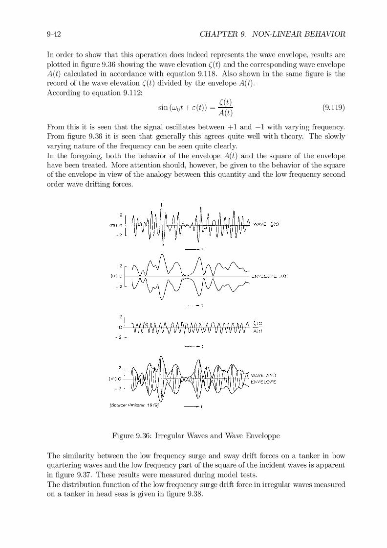
9-42 CHAPTER 9. NON-LINEAR BEHAVIOR
In order to show that this operation does indeed represents the wave envelope, results areplotted in …gure 9.36 showing the wave elevation ³(t) and the corresponding wave envelopeA(t) calculated in accordance with equation 9.118. Also shown in the same …gure is therecord of the wave elevation ³(t) divided by the envelope A(t).According to equation 9.112:
sin (!0t+ "(t)) =³(t)
A(t)(9.119)
From this it is seen that the signal oscillates between +1 and ¡1 with varying frequency.From …gure 9.36 it is seen that generally this agrees quite well with theory. The slowlyvarying nature of the frequency can be seen quite clearly.In the foregoing, both the behavior of the envelope A(t) and the square of the envelopehave been treated. More attention should, however, be given to the behavior of the squareof the envelope in view of the analogy between this quantity and the low frequency secondorder wave drifting forces.
Figure 9.36: Irregular Waves and Wave Enveloppe
The similarity between the low frequency surge and sway drift forces on a tanker in bowquartering waves and the low frequency part of the square of the incident waves is apparentin …gure 9.37. These results were measured during model tests.The distribution function of the low frequency surge drift force in irregular waves measuredon a tanker in head seas is given in …gure 9.38.
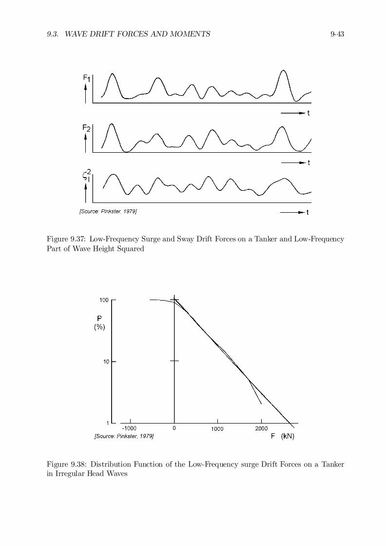
9.3. WAVE DRIFT FORCES AND MOMENTS 9-43
Figure 9.37: Low-Frequency Surge and Sway Drift Forces on a Tanker and Low-FrequencyPart of Wave Height Squared
Figure 9.38: Distribution Function of the Low-Frequency surge Drift Forces on a Tankerin Irregular Head Waves
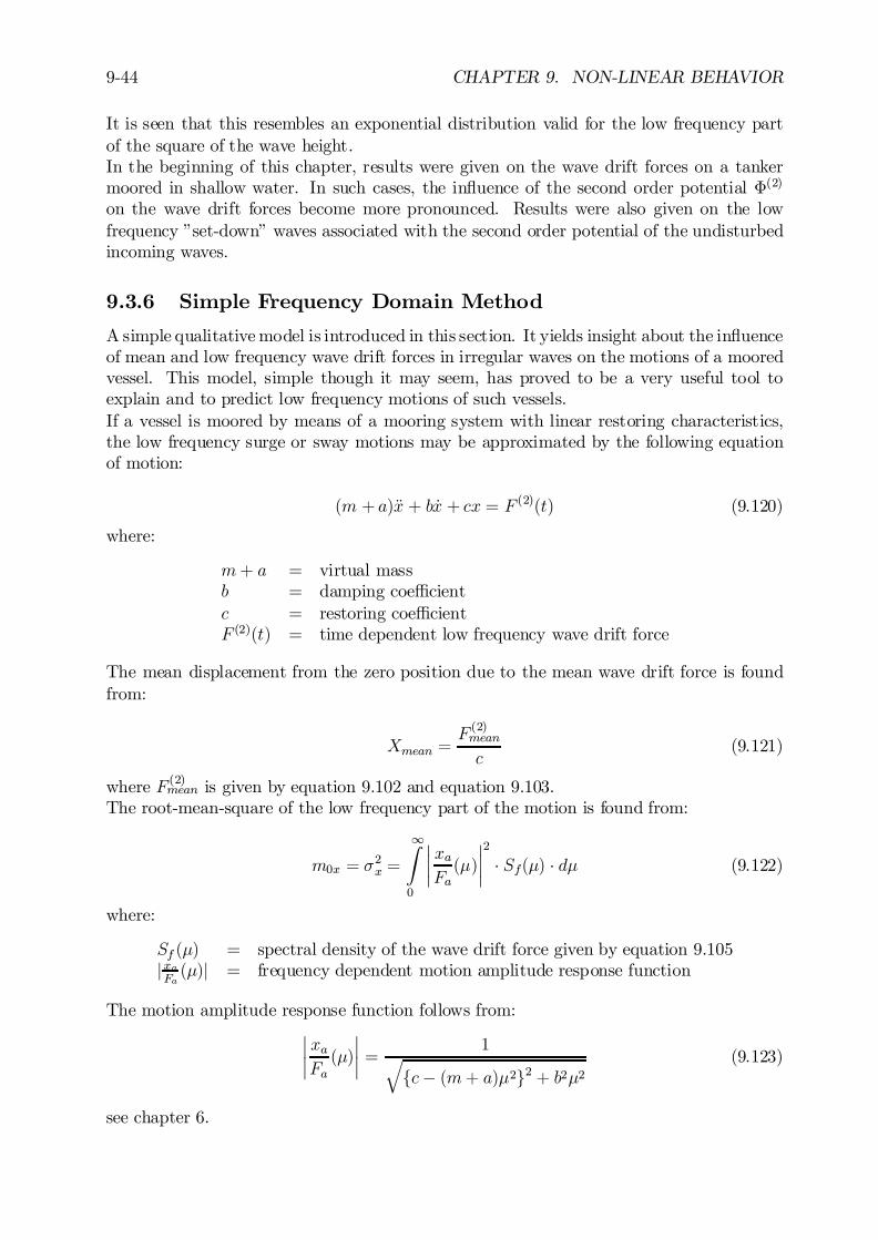
9-44 CHAPTER 9. NON-LINEAR BEHAVIOR
It is seen that this resembles an exponential distribution valid for the low frequency partof the square of the wave height.In the beginning of this chapter, results were given on the wave drift forces on a tankermoored in shallow water. In such cases, the in‡uence of the second order potential ©(2)
on the wave drift forces become more pronounced. Results were also given on the lowfrequency ”set-down” waves associated with the second order potential of the undisturbedincoming waves.
9.3.6 Simple Frequency Domain Method
A simple qualitative model is introduced in this section. It yields insight about the in‡uenceof mean and low frequency wave drift forces in irregular waves on the motions of a mooredvessel. This model, simple though it may seem, has proved to be a very useful tool toexplain and to predict low frequency motions of such vessels.If a vessel is moored by means of a mooring system with linear restoring characteristics,the low frequency surge or sway motions may be approximated by the following equationof motion:
(m + a)Äx + b _x + cx = F (2)(t) (9.120)
where:
m+ a = virtual massb = damping coe¢cientc = restoring coe¢cientF (2)(t) = time dependent low frequency wave drift force
The mean displacement from the zero position due to the mean wave drift force is foundfrom:
Xmean =F (2)meanc
(9.121)
where F (2)mean is given by equation 9.102 and equation 9.103.The root-mean-square of the low frequency part of the motion is found from:
m0x = ¾2x =
1Z
0
¯¯ xaFa(¹)
¯¯2
¢ Sf(¹) ¢ d¹ (9.122)
where:
Sf (¹) = spectral density of the wave drift force given by equation 9.105jxaFa(¹)j = frequency dependent motion amplitude response function
The motion amplitude response function follows from:¯¯ xaFa(¹)
¯¯ = 1q
fc¡ (m+ a)¹2g2 + b2¹2(9.123)
see chapter 6.
9.3. WAVE DRIFT FORCES AND MOMENTS 9-45
For slightly damped systems, which applies to many cases of moored vessels, the followingassumption may be made with respect to the spectral density of the low frequency driftforce:
Sf(¹) t Sf (¹e) (9.124)
where ¹e is the natural frequency of the moored vessel de…ned by:
¹e =
rc
m+ a(9.125)
This result implies that the major part of the motion response will be due to excitationnear the natural frequency. In that case, equation 9.122 may be approximated by:
¾2x = Sf(¹e) ¢1Z
0
¯¯ xaFa(¹)
¯¯2
¢ d¹ (9.126)
If the natural frequency of the system is close to zero, the following approximation can alsobe applied:
Sf(¹e) t Sf(0) (9.127)
From equation 9.105 it follows that:
Sf(0) = 8
1Z
0
S2³ (!) ¢ jT (!; !)j2 ¢ d! (9.128)
Since Q(!;!) = 0 (from equation 9.98) and taking into account equation 9.103 this be-comes:
Sf (0) = 8
1Z
0
S2³ (!) ¢¯¯F³2a(!)
¯¯2
¢ d! (9.129)
In this case the mean-square of the low frequency part of the motions can be written asfollows:
¾2x = Sf(0)
1Z
0
¯¯ xaFa(¹)
¯¯2
¢ d¹ (9.130)
Taking into account equation 9.123 this becomes:
¾2x =¼
2bc¢ Sf(0) (9.131)
which reveals the remarkable fact that the virtual mass (m+a) of the vessels has no directbearing on the mean or the low frequency motion.From equation 9.131, it is seen that besides the exciting force, the most important fac-tors determining the motions appear to be the damping b and the sti¤ness c of themooring system. The trend suggested by equation 9.131 is also seen in results given by[Remery and Hermans, 1972] on the in‡uence of the parameter c on the RMS value of thelow frequency surge motion of a barge moored in head seas.The general characteristic of the mooring force as expressed by the mean-square of themooring force cx is found by multiplying equation 9.131 by c2:
9-46 CHAPTER 9. NON-LINEAR BEHAVIOR
¾2mf =¼c
2b¢ Sf(0) (9.132)
This reveals that as the sti¤ness c of a mooring system increases, so does the RMS valueof the low frequency mooring force.It must be remembered that equations 9.131 and 9.132 can only be used in an indicativeway. In many cases the mooring system will not be linear, or the number of degreesof freedom of the moored vessel will be too great to allow such simpli…cations as madehere. We refer to [Oortmerssen, 1976b] and [Wichers, 1988] for more details concerningsimulation techniques for moored vessels.
9.4 Remarks
The theory relating to second order wave drift forces has been treated in this chapter.Some results of computations have been compared with results derived analytically and bymeans of model tests. These results apply to the mean drift forces in regular waves, whichcan be used to estimate the mean and low frequency drift forces in irregular waves.The low frequency part of the wave drift forces should theoretically, be determined by con-sidering the drift forces in regular wave groups. In such cases the second order potential alsocontributes to the force, see [Pinkster, 1980]. [Faltinsen and Loken, 1979] have indicatedthat, for vessels ‡oating in beam seas, the sway drift forces calculated using only informa-tion on the mean drift forces in regular waves gives results which are su¢ciently accuratefor engineering purposes. Results given by [Pinkster and Hooft, 1978] and [Pinkster, 1979]on the low frequency drift forces on a barge and a semi-submersible in head waves gen-erally con…rms the conclusion provided the frequency of interest is low. Frequencies ofinterest for moored vessels are the natural frequencies of the horizontal motions inducedby the presence of the mooring system. In some cases the natural frequencies of verticalmotions can also be of interest from the point of view of vertical motions induced by thelow frequency wave drift forces.It can be shown that, in at least one case, the mean wave drift forces in regular wavescannot be used to estimate the low frequency drift forces in irregular waves. This caseconcerns the low frequency sway drift force on a free ‡oating, submerged cylinder in beamseas. According to [Ogilvie, 1963], the mean wave drift force in regular waves is zero forall wave frequencies. This means that the low frequency wave drift force in irregular wavesestimated using only the mean wave drift force will be zero as well. Computations carriedout using the method given by [Pinkster, 1979] which determines the low frequency force inregular wave groups show that this will not be true. The table below presents amplitudesof low-frequency sway drift forces in regular wave groups on a submerged cylinder in beamwaves, with its center one diameter below the mean free surface:
F2ij¼½gL³1³2
2kih2kjh 2 4 6 8
2 0.00 0.08 0.09 0.084 0.00 0.06 0.076 0.00 0.058 0.00
Chapter 10
STATION KEEPING
10.1 Introduction
Precise positioning and long term motion control of ships and other ‡oating structuresare important in o¤shore operations. Mooring systems and thrusters are major tools formaintaining a structure in position in current, wind and waves. The increasing applicationof large o¤shore structures has put high demands upon the design of these positioningarrangements. Important parameters in this respect are the large displacement of thestructure, deep and hostile waters and the required round-the-year workability.The external loads on the structure have been discussed in earlier chapters. This chaptertreats some other important phenomena of station keeping problems of a ‡oating structure,such as mooring systems, thruster performance and motion control.
10.2 Mooring Systems
Any mooring system is made of a number of lines (chain, wire or synthetic rope) withtheir upper ends attached to di¤erent points of the ‡oating structure and their lower endsanchored at the sea bed.The cables are constructed from steel chain, rope or a combination of both. The ropesare available in constructions from steel and natural or synthetic …bres. Multi-componentcable lines - cables composed of two or more lengths of di¤erent material - are used to geta heavy chain at the sea bed and a lighter rope close to the water surface. This results inan optimal combination of sti¤ness and total weight. The tension forces in the cables aredependent on the cable weight, its elastic properties and the mooring system.
Typical and important types of mooring systems are:
² Catenary Line MooringThis are the oldest and still most common mooring systems. It derives its restoringforce primarily by lifting and lowering the weight of the mooring line, at least in thestatic sense. Generally, this yields a hard spring system with a force increasing morethan directly proportional to the displacement. In a spread mooring system as givenin …gure 10.1, several pre-tension anchor lines are arrayed around the structure to
0J.M.J. Journée and W.W. Massie, ”OFFSHORE HYDROMECHANICS”, First Edition, January 2001,Delft University of Technology. For updates see web site: http://www.shipmotions.nl.
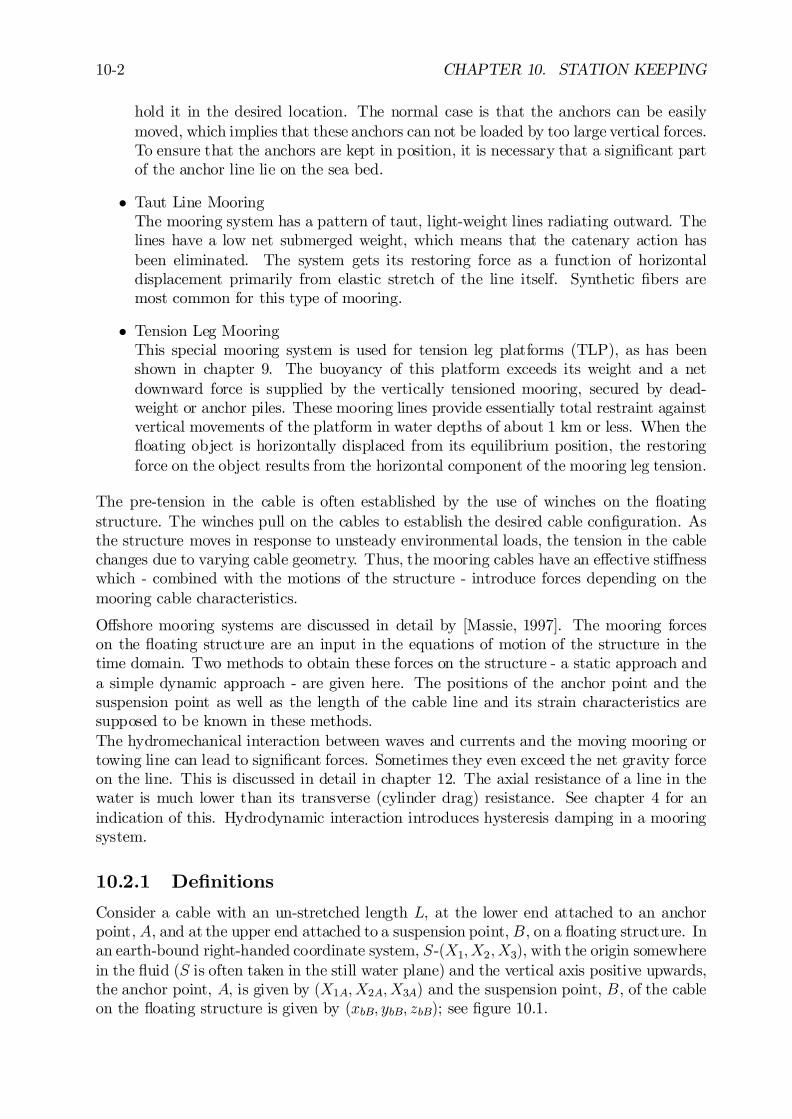
10-2 CHAPTER 10. STATION KEEPING
hold it in the desired location. The normal case is that the anchors can be easilymoved, which implies that these anchors can not be loaded by too large vertical forces.To ensure that the anchors are kept in position, it is necessary that a signi…cant partof the anchor line lie on the sea bed.
² Taut Line MooringThe mooring system has a pattern of taut, light-weight lines radiating outward. Thelines have a low net submerged weight, which means that the catenary action hasbeen eliminated. The system gets its restoring force as a function of horizontaldisplacement primarily from elastic stretch of the line itself. Synthetic …bers aremost common for this type of mooring.
² Tension Leg MooringThis special mooring system is used for tension leg platforms (TLP), as has beenshown in chapter 9. The buoyancy of this platform exceeds its weight and a netdownward force is supplied by the vertically tensioned mooring, secured by dead-weight or anchor piles. These mooring lines provide essentially total restraint againstvertical movements of the platform in water depths of about 1 km or less. When the‡oating object is horizontally displaced from its equilibrium position, the restoringforce on the object results from the horizontal component of the mooring leg tension.
The pre-tension in the cable is often established by the use of winches on the ‡oatingstructure. The winches pull on the cables to establish the desired cable con…guration. Asthe structure moves in response to unsteady environmental loads, the tension in the cablechanges due to varying cable geometry. Thus, the mooring cables have an e¤ective sti¤nesswhich - combined with the motions of the structure - introduce forces depending on themooring cable characteristics.
O¤shore mooring systems are discussed in detail by [Massie, 1997]. The mooring forceson the ‡oating structure are an input in the equations of motion of the structure in thetime domain. Two methods to obtain these forces on the structure - a static approach anda simple dynamic approach - are given here. The positions of the anchor point and thesuspension point as well as the length of the cable line and its strain characteristics aresupposed to be known in these methods.The hydromechanical interaction between waves and currents and the moving mooring ortowing line can lead to signi…cant forces. Sometimes they even exceed the net gravity forceon the line. This is discussed in detail in chapter 12. The axial resistance of a line in thewater is much lower than its transverse (cylinder drag) resistance. See chapter 4 for anindication of this. Hydrodynamic interaction introduces hysteresis damping in a mooringsystem.
10.2.1 De…nitions
Consider a cable with an un-stretched length L, at the lower end attached to an anchorpoint, A, and at the upper end attached to a suspension point,B, on a ‡oating structure. Inan earth-bound right-handed coordinate system, S-(X1; X2; X3), with the origin somewherein the ‡uid (S is often taken in the still water plane) and the vertical axis positive upwards,the anchor point, A, is given by (X1A; X2A; X3A) and the suspension point, B, of the cableon the ‡oating structure is given by (xbB; ybB; zbB); see …gure 10.1.
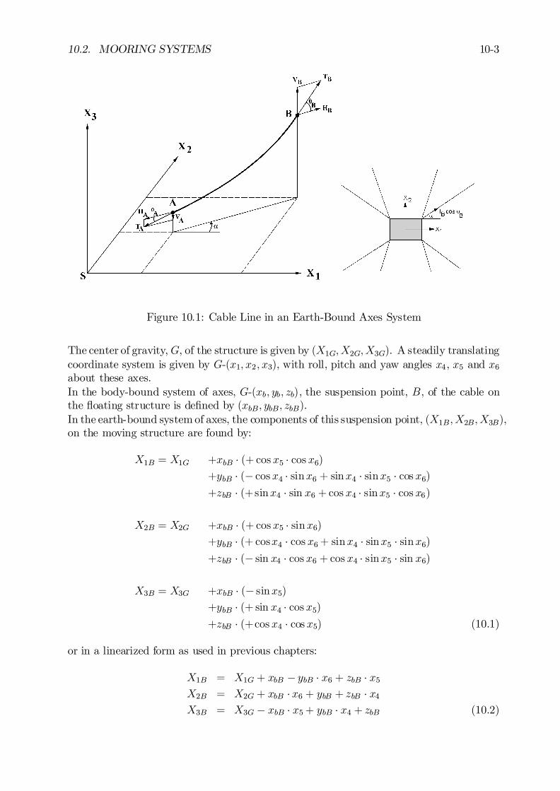
10.2. MOORING SYSTEMS 10-3
Figure 10.1: Cable Line in an Earth-Bound Axes System
The center of gravity,G, of the structure is given by (X1G; X2G; X3G). A steadily translatingcoordinate system is given by G-(x1; x2; x3), with roll, pitch and yaw angles x4, x5 and x6about these axes.In the body-bound system of axes, G-(xb; yb; zb), the suspension point, B, of the cable onthe ‡oating structure is de…ned by (xbB; ybB; zbB).In the earth-bound system of axes, the components of this suspension point, (X1B; X2B; X3B),on the moving structure are found by:
X1B = X1G +xbB ¢ (+ cos x5 ¢ cos x6)+ybB ¢ (¡ cos x4 ¢ sinx6 + sinx4 ¢ sinx5 ¢ cos x6)+zbB ¢ (+sinx4 ¢ sin x6 +cos x4 ¢ sinx5 ¢ cos x6)
X2B = X2G +xbB ¢ (+ cos x5 ¢ sinx6)+ybB ¢ (+ cosx4 ¢ cos x6+ sinx4 ¢ sinx5 ¢ sinx6)+zbB ¢ (¡ sin x4 ¢ cos x6 +cos x4 ¢ sinx5 ¢ sin x6)
X3B = X3G +xbB ¢ (¡ sinx5)+ybB ¢ (+ sin x4 ¢ cos x5)+zbB ¢ (+cos x4 ¢ cos x5) (10.1)
or in a linearized form as used in previous chapters:
X1B = X1G + xbB ¡ ybB ¢ x6 + zbB ¢ x5X2B = X2G + xbB ¢x6 + ybB + zbB ¢ x4X3B = X3G ¡ xbB ¢ x5+ ybB ¢ x4 + zbB (10.2)

10-4 CHAPTER 10. STATION KEEPING
10.2.2 Static Catenary Line
Consider now this cable with an un-stretched length L, at the lower end attached to ananchor point, A, and at the upper end attached to a suspension point, B, in a verticalplane through this cable line. A two-dimensional sketch of this catenary anchor line isshown in …gure 10.2.
Figure 10.2: Cable Curve Symbols
For obtaining the equations of a static cable line, reference can be given to a number ofpapers in this …eld; for instance [Massie, 1997] and [Korkut and Hebert, 1970].
Inelastic Cable Line
Suppose: the length of the cable, L, is known and the relative positions of two - in principlearbitrary - points A and B on the cable are de…ned by the distances k and h. The anchorpoint is de…ned in a new 2-D coordinate system (see …gure 10.2) by (xA; zA) and thesuspension point on the structure is de…ned by (xB; zB) with:
xB = xA+ k and zB = zA+ h (10.3)
The position of the origin of the axis system (x; z) relative to the cable line follows fromtwo unknown coe¢cients, C1 and C2, as will be explained in the following.When de…ning:
u =dz
dxand c =
H0w
(10.4)
in which w is the weight per unit length of the cable in water (see also …gure 10.2-a), itcan be found that:
ds =p1 + u2 ¢ dx
10.2. MOORING SYSTEMS 10-5
du = d
µdz
dx
¶= d (tanÁ) =
w ¢ dsH0
=ds
c
du =
p1 + u2
c¢ dx or: dx = c ¢ dup
1 + u2(10.5)
With this, an integral equation will be obtained:Zdx = c ¢
Zdup1 + u2
(10.6)
Integration of this equation provides:
x = c ¢ ln³u+
p1 + u2
´+ C1 =
c
sinh u+C1 (10.7)
or:u = sinh
³xc
¡ C1´
(10.8)
Herein, the constant C1 will be zero because the origin in …gure 10.2 is chosen in such away that the derivative u = dz=dx is zero for x is zero, so:
u = sinh³xc
´(10.9)
Then the equation of the cable curve can be written as:
z =
xZ
0
u ¢ dx = c ¢ cosh³xc
´+ C2 (10.10)
The origin in …gure 10.2 is chosen in such a way that C2 = 0, thus:
z = c ¢ cosh³xc
´(10.11)
This means that z = c for x = 0.Also, the distance s can be obtained:
s =
xZ
0
p1 + u2 ¢ dx =
xZ
0
r1 + sinh2
³xc
´¢ dx (10.12)
or:s = c ¢ sinh
³xc
´(10.13)
Combining equations 10.11 and 10.13 provides a simple relation between z and s:
z2 ¡ s2 = c2 (10.14)
from which after some algebra for the points A and B on the cable line follows:
pL2¡ h2 = c
p2 ¢ sinh
µk
2c
¶(10.15)
The values k, h and L are known, so the value of c has to be found from this equation inan iterative manner.
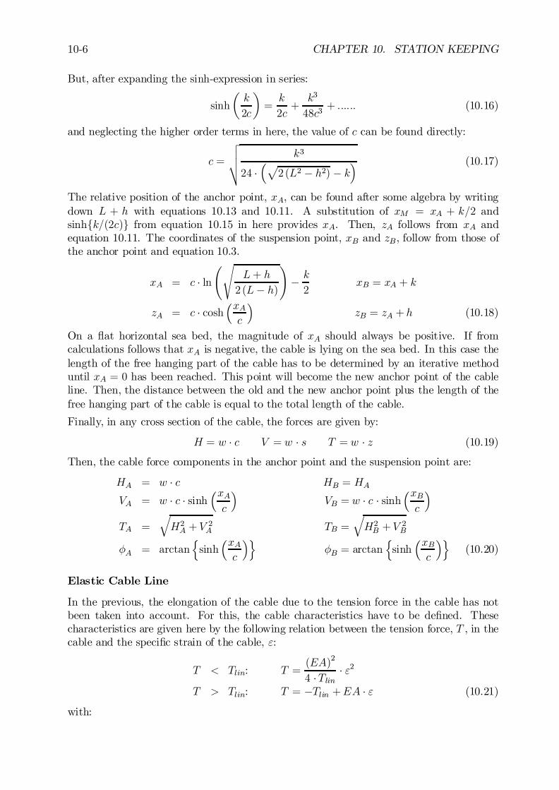
10-6 CHAPTER 10. STATION KEEPING
But, after expanding the sinh-expression in series:
sinh
µk
2c
¶=k
2c+k3
48c3+ :::::: (10.16)
and neglecting the higher order terms in here, the value of c can be found directly:
c =
vuut k3
24 ¢³p
2 (L2 ¡ h2) ¡ k´ (10.17)
The relative position of the anchor point, xA, can be found after some algebra by writingdown L + h with equations 10.13 and 10.11. A substitution of xM = xA + k=2 andsinhfk=(2c)g from equation 10.15 in here provides xA. Then, zA follows from xA andequation 10.11. The coordinates of the suspension point, xB and zB, follow from those ofthe anchor point and equation 10.3.
xA = c ¢ lnÃs
L+ h
2 (L¡ h)
!¡ k
2xB = xA + k
zA = c ¢ cosh³xAc
´zB = zA + h (10.18)
On a ‡at horizontal sea bed, the magnitude of xA should always be positive. If fromcalculations follows that xA is negative, the cable is lying on the sea bed. In this case thelength of the free hanging part of the cable has to be determined by an iterative methoduntil xA = 0 has been reached. This point will become the new anchor point of the cableline. Then, the distance between the old and the new anchor point plus the length of thefree hanging part of the cable is equal to the total length of the cable.
Finally, in any cross section of the cable, the forces are given by:
H = w ¢ c V = w ¢ s T = w ¢ z (10.19)
Then, the cable force components in the anchor point and the suspension point are:
HA = w ¢ c HB = HA
VA = w ¢ c ¢ sinh³xAc
´VB = w ¢ c ¢ sinh
³xBc
´
TA =qH2A + V
2A TB =
qH2B + V
2B
ÁA = arctannsinh
³xAc
´oÁB = arctan
nsinh
³xBc
´o(10.20)
Elastic Cable Line
In the previous, the elongation of the cable due to the tension force in the cable has notbeen taken into account. For this, the cable characteristics have to be de…ned. Thesecharacteristics are given here by the following relation between the tension force, T , in thecable and the speci…c strain of the cable, ":
T < Tlin: T =(EA)2
4 ¢Tlin¢ "2
T > Tlin: T = ¡Tlin +EA ¢ " (10.21)
with:
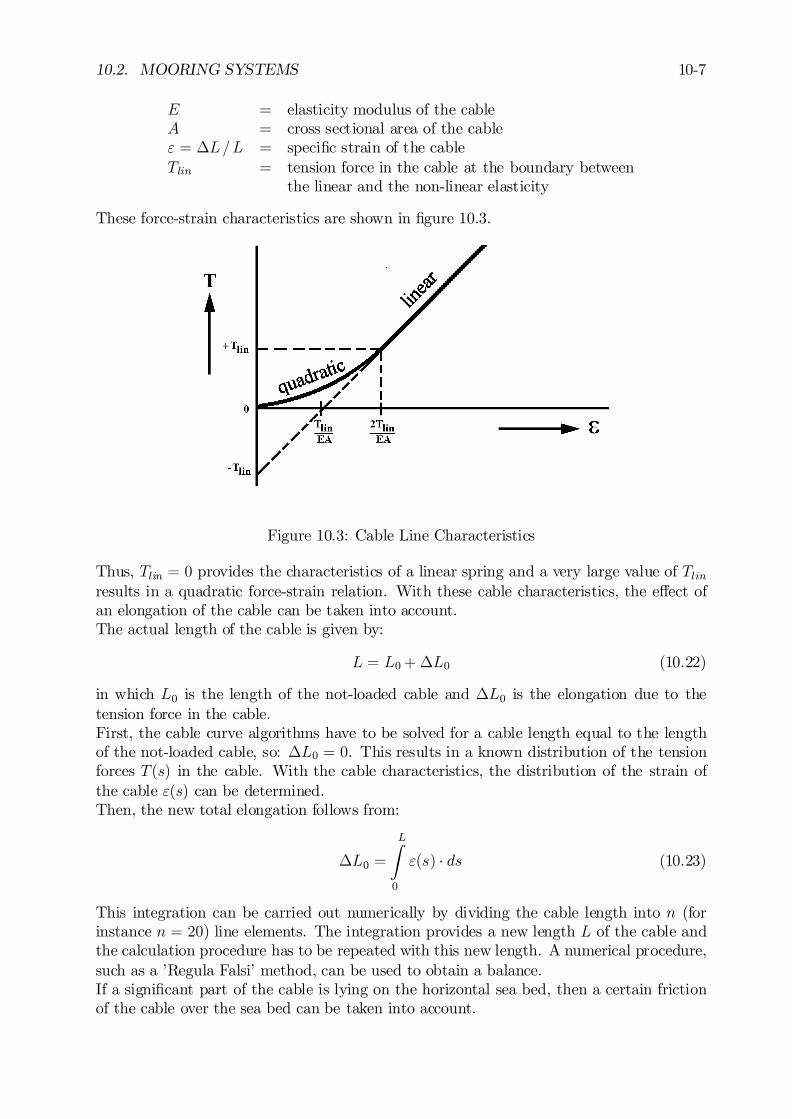
10.2. MOORING SYSTEMS 10-7
E = elasticity modulus of the cableA = cross sectional area of the cable" = ¢L=L = speci…c strain of the cableTlin = tension force in the cable at the boundary between
the linear and the non-linear elasticity
These force-strain characteristics are shown in …gure 10.3.
Figure 10.3: Cable Line Characteristics
Thus, Tlin = 0 provides the characteristics of a linear spring and a very large value of Tlinresults in a quadratic force-strain relation. With these cable characteristics, the e¤ect ofan elongation of the cable can be taken into account.The actual length of the cable is given by:
L = L0+ ¢L0 (10.22)
in which L0 is the length of the not-loaded cable and ¢L0 is the elongation due to thetension force in the cable.First, the cable curve algorithms have to be solved for a cable length equal to the lengthof the not-loaded cable, so: ¢L0 = 0. This results in a known distribution of the tensionforces T(s) in the cable. With the cable characteristics, the distribution of the strain ofthe cable "(s) can be determined.Then, the new total elongation follows from:
¢L0 =
LZ
0
"(s) ¢ ds (10.23)
This integration can be carried out numerically by dividing the cable length into n (forinstance n = 20) line elements. The integration provides a new length L of the cable andthe calculation procedure has to be repeated with this new length. A numerical procedure,such as a ’Regula Falsi’ method, can be used to obtain a balance.If a signi…cant part of the cable is lying on the horizontal sea bed, then a certain frictionof the cable over the sea bed can be taken into account.
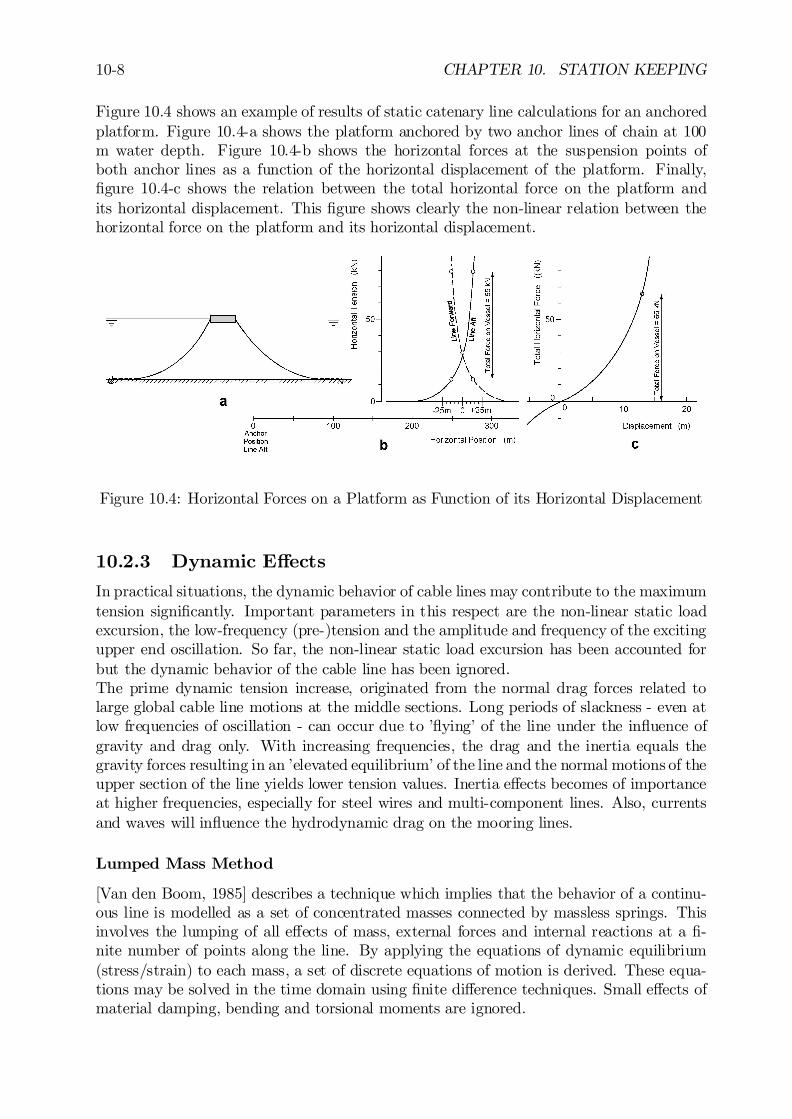
10-8 CHAPTER 10. STATION KEEPING
Figure 10.4 shows an example of results of static catenary line calculations for an anchoredplatform. Figure 10.4-a shows the platform anchored by two anchor lines of chain at 100m water depth. Figure 10.4-b shows the horizontal forces at the suspension points ofboth anchor lines as a function of the horizontal displacement of the platform. Finally,…gure 10.4-c shows the relation between the total horizontal force on the platform andits horizontal displacement. This …gure shows clearly the non-linear relation between thehorizontal force on the platform and its horizontal displacement.
Figure 10.4: Horizontal Forces on a Platform as Function of its Horizontal Displacement
10.2.3 Dynamic E¤ects
In practical situations, the dynamic behavior of cable lines may contribute to the maximumtension signi…cantly. Important parameters in this respect are the non-linear static loadexcursion, the low-frequency (pre-)tension and the amplitude and frequency of the excitingupper end oscillation. So far, the non-linear static load excursion has been accounted forbut the dynamic behavior of the cable line has been ignored.The prime dynamic tension increase, originated from the normal drag forces related tolarge global cable line motions at the middle sections. Long periods of slackness - even atlow frequencies of oscillation - can occur due to ’‡ying’ of the line under the in‡uence ofgravity and drag only. With increasing frequencies, the drag and the inertia equals thegravity forces resulting in an ’elevated equilibrium’ of the line and the normal motions of theupper section of the line yields lower tension values. Inertia e¤ects becomes of importanceat higher frequencies, especially for steel wires and multi-component lines. Also, currentsand waves will in‡uence the hydrodynamic drag on the mooring lines.
Lumped Mass Method
[Van den Boom, 1985] describes a technique which implies that the behavior of a continu-ous line is modelled as a set of concentrated masses connected by massless springs. Thisinvolves the lumping of all e¤ects of mass, external forces and internal reactions at a …-nite number of points along the line. By applying the equations of dynamic equilibrium(stress/strain) to each mass, a set of discrete equations of motion is derived. These equa-tions may be solved in the time domain using …nite di¤erence techniques. Small e¤ects ofmaterial damping, bending and torsional moments are ignored.
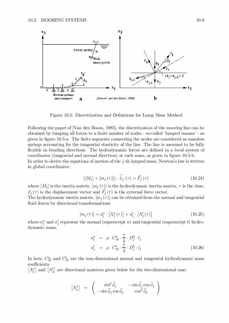
10.2. MOORING SYSTEMS 10-9
Figure 10.5: Discretization and De…nitions for Lump Mass Method
Following the paper of [Van den Boom, 1985], the discretization of the mooring line can beobtained by lumping all forces to a …nite number of nodes - so-called ’lumped masses’ - asgiven in …gure 10.5-a. The …nite segments connecting the nodes are considered as masslesssprings accounting for the tangential elasticity of the line. The line is assumed to be fully‡exible in bending directions. The hydrodynamic forces are de…ned in a local system ofcoordinates (tangential and normal direction) at each mass, as given in …gure 10.5-b.In order to derive the equations of motion of the j-th lumped mass, Newton’s law is writtenin global coordinates:
([Mj] + [mj (¿ )]) ¢!Äxj (¿) = ~Fj (¿) (10.24)
where [Mj] is the inertia matrix, [mj (¿)] is the hydrodynamic inertia matrix, ¿ is the time,~xj (¿ ) is the displacement vector and ~Fj (¿) is the external force vector.The hydrodynamic inertia matrix, [mj (¿ )] can be obtained from the normal and tangential‡uid forces by directional transformations:
[mj (¿ )] = anj ¢
£¤nj (¿ )
¤+ atj ¢
£¤tj (¿ )
¤(10.25)
where anj and atj represent the normal (superscript n) and tangential (superscript t) hydro-dynamic mass:
anj = ½ ¢ CnM ¢ ¼4
¢D2j ¢ lj
atj = ½ ¢ CtM ¢ ¼4
¢D2j ¢ lj (10.26)
In here, CnM and CtM are the non-dimensional normal and tangential hydrodynamic masscoe¢cients.£¤nj
¤and
£¤tj
¤are directional matrices given below for the two-dimensional case:
£¤nj
¤=
Ãsin2 ~Áj ¡ sin~Áj cos~Áj
¡ sin~Áj cos ~Áj cos2~Áj
!
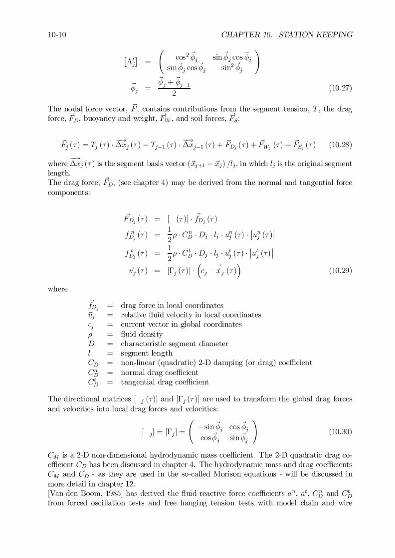
10-10 CHAPTER 10. STATION KEEPING
£¤tj
¤=
Ãcos2~Áj sin~Áj cos~Áj
sin~Áj cos ~Áj sin2 ~Áj
!
~Áj =~Áj + ~Áj¡1
2(10.27)
The nodal force vector, ~F , contains contributions from the segment tension, T , the dragforce, ~FD, buoyancy and weight, ~FW , and soil forces, ~FS:
~Fj (¿) = Tj (¿) ¢ ¡!¢xj (¿ ) ¡ Tj¡1 (¿) ¢ ¡!
¢xj¡1 (¿) + ~FDj (¿) + ~FWj (¿) + ~FSj (¿ ) (10.28)
where¡!¢xj (¿ ) is the segment basis vector (~xj+1 ¡ ~xj) =lj, in which lj is the original segment
length.The drag force, ~FD, (see chapter 4) may be derived from the normal and tangential forcecomponents:
~FDj (¿ ) = [ (¿ )] ¢ ~fDj (¿ )
f nDj (¿ ) =1
2½ ¢ CnD ¢Dj ¢ lj ¢ unj (¿) ¢
¯unj (¿ )
¯
f tDj (¿ ) =1
2½ ¢ C tD ¢Dj ¢ lj ¢ utj (¿ ) ¢
¯utj (¿)
¯
~uj (¿ ) = [¡j (¿ )] ¢³cj¡
!_xj (¿ )
´(10.29)
where
~fDj = drag force in local coordinates~uj = relative ‡uid velocity in local coordinatescj = current vector in global coordinates½ = ‡uid densityD = characteristic segment diameterl = segment lengthCD = non-linear (quadratic) 2-D damping (or drag) coe¢cientCnD = normal drag coe¢cientCtD = tangential drag coe¢cient
The directional matrices [j (¿)] and [¡j (¿ )] are used to transform the global drag forcesand velocities into local drag forces and velocities:
[j] = [¡j] =
á sin~Áj cos ~Ájcos~Áj sin~Áj
!(10.30)
CM is a 2-D non-dimensional hydrodynamic mass coe¢cient. The 2-D quadratic drag co-e¢cient CD has been discussed in chapter 4. The hydrodynamic mass and drag coe¢cientsCM and CD - as they are used in the so-called Morison equations - will be discussed inmore detail in chapter 12.[Van den Boom, 1985] has derived the ‡uid reactive force coe¢cients an, at, CnD and CtDfrom forced oscillation tests and free hanging tension tests with model chain and wire
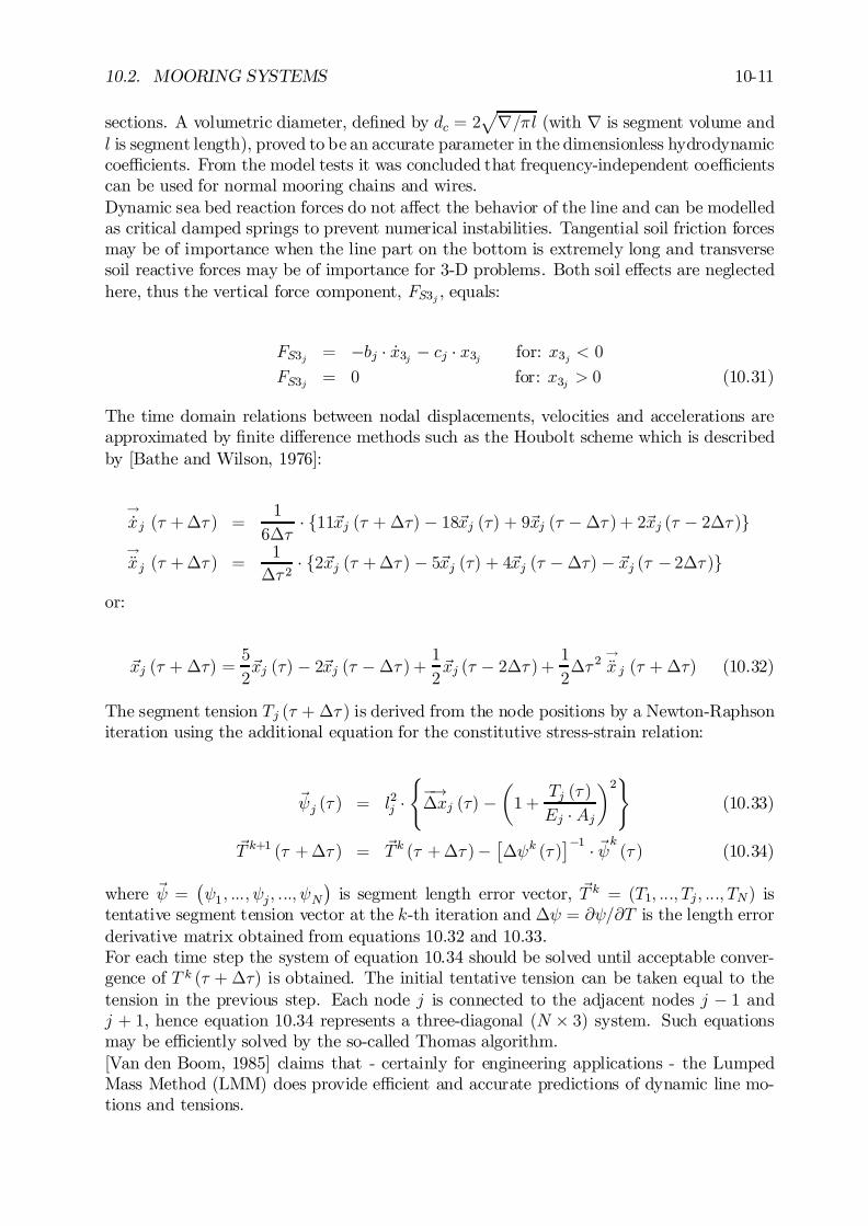
10.2. MOORING SYSTEMS 10-11
sections. A volumetric diameter, de…ned by dc = 2p
r=¼l (with r is segment volume andl is segment length), proved to be an accurate parameter in the dimensionless hydrodynamiccoe¢cients. From the model tests it was concluded that frequency-independent coe¢cientscan be used for normal mooring chains and wires.Dynamic sea bed reaction forces do not a¤ect the behavior of the line and can be modelledas critical damped springs to prevent numerical instabilities. Tangential soil friction forcesmay be of importance when the line part on the bottom is extremely long and transversesoil reactive forces may be of importance for 3-D problems. Both soil e¤ects are neglectedhere, thus the vertical force component, FS3j , equals:
FS3j = ¡bj ¢ _x3j ¡ cj ¢ x3j for: x3j < 0
FS3j = 0 for: x3j > 0 (10.31)
The time domain relations between nodal displacements, velocities and accelerations areapproximated by …nite di¤erence methods such as the Houbolt scheme which is describedby [Bathe and Wilson, 1976]:
!_xj (¿ +¢¿ ) =
1
6¢¿¢ f11~xj (¿ + ¢¿) ¡ 18~xj (¿) + 9~xj (¿ ¡¢¿ ) + 2~xj (¿ ¡ 2¢¿ )g
!Äxj (¿ +¢¿ ) =
1
¢¿ 2¢ f2~xj (¿ +¢¿ ) ¡ 5~xj (¿) + 4~xj (¿ ¡¢¿) ¡ ~xj (¿ ¡ 2¢¿ )g
or:
~xj (¿ + ¢¿) =5
2~xj (¿) ¡ 2~xj (¿ ¡¢¿ ) + 1
2~xj (¿ ¡ 2¢¿ ) + 1
2¢¿ 2
!Äx j (¿ + ¢¿) (10.32)
The segment tension Tj (¿ + ¢¿ ) is derived from the node positions by a Newton-Raphsoniteration using the additional equation for the constitutive stress-strain relation:
~Ãj (¿ ) = l2j ¢(
¡!¢xj (¿) ¡
µ1 +
Tj (¿ )
Ej ¢ Aj
¶2)
(10.33)
~T k+1 (¿ +¢¿ ) = ~Tk (¿ +¢¿ )¡£¢Ãk (¿ )
¤¡1 ¢ ~Ãk (¿ ) (10.34)
where ~Ã =¡Ã1; :::; Ãj; :::; ÃN
¢is segment length error vector, ~T k = (T1; :::; Tj; :::; TN) is
tentative segment tension vector at the k-th iteration and ¢Ã = @Ã=@T is the length errorderivative matrix obtained from equations 10.32 and 10.33.For each time step the system of equation 10.34 should be solved until acceptable conver-gence of T k (¿ + ¢¿) is obtained. The initial tentative tension can be taken equal to thetension in the previous step. Each node j is connected to the adjacent nodes j ¡ 1 andj + 1, hence equation 10.34 represents a three-diagonal (N £ 3) system. Such equationsmay be e¢ciently solved by the so-called Thomas algorithm.[Van den Boom, 1985] claims that - certainly for engineering applications - the LumpedMass Method (LMM) does provide e¢cient and accurate predictions of dynamic line mo-tions and tensions.
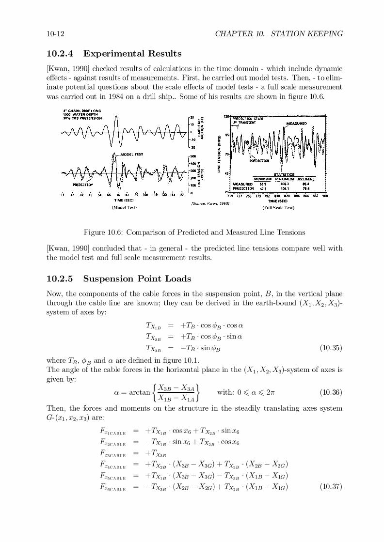
10-12 CHAPTER 10. STATION KEEPING
10.2.4 Experimental Results
[Kwan, 1990] checked results of calculations in the time domain - which include dynamice¤ects - against results of measurements. First, he carried out model tests. Then, - to elim-inate potential questions about the scale e¤ects of model tests - a full scale measurementwas carried out in 1984 on a drill ship.. Some of his results are shown in …gure 10.6.
Figure 10.6: Comparison of Predicted and Measured Line Tensions
[Kwan, 1990] concluded that - in general - the predicted line tensions compare well withthe model test and full scale measurement results.
10.2.5 Suspension Point Loads
Now, the components of the cable forces in the suspension point, B, in the vertical planethrough the cable line are known; they can be derived in the earth-bound (X1;X2; X3)-system of axes by:
TX1B = +TB ¢ cos ÁB ¢ cos®TX2B = +TB ¢ cos ÁB ¢ sin®TX3B = ¡TB ¢ sinÁB (10.35)
where TB, ÁB and ® are de…ned in …gure 10.1.The angle of the cable forces in the horizontal plane in the (X1; X2; X3)-system of axes isgiven by:
® = arctan
½X3B ¡X3AX1B ¡X1A
¾with: 0 6 ® 6 2¼ (10.36)
Then, the forces and moments on the structure in the steadily translating axes systemG-(x1; x2; x3) are:
Fx1CAB LE = +TX1B ¢ cos x6 + TX2B ¢ sinx6Fx2CAB LE = ¡TX1B ¢ sin x6 + TX2B ¢ cosx6Fx3CAB LE = +TX3BFx4CAB LE
= +TX2B ¢ (X3B ¡X3G) + TX3B ¢ (X2B ¡X2G)Fx5CAB LE = +TX1B ¢ (X3B ¡X3G) ¡ TX3B ¢ (X1B ¡X1G)Fx6CAB LE = ¡TX3B ¢ (X2B ¡X2G) + TX2B ¢ (X1B ¡X1G) (10.37)
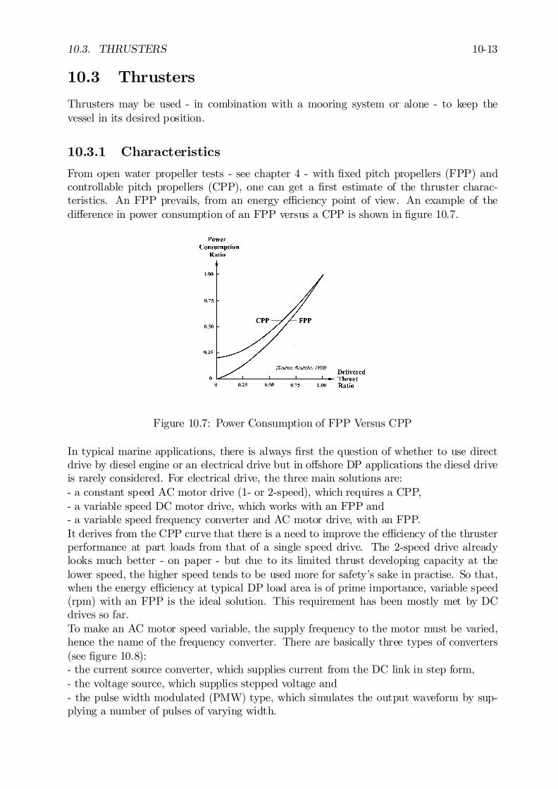
10.3. THRUSTERS 10-13
10.3 Thrusters
Thrusters may be used - in combination with a mooring system or alone - to keep thevessel in its desired position.
10.3.1 Characteristics
From open water propeller tests - see chapter 4 - with …xed pitch propellers (FPP) andcontrollable pitch propellers (CPP), one can get a …rst estimate of the thruster charac-teristics. An FPP prevails, from an energy e¢ciency point of view. An example of thedi¤erence in power consumption of an FPP versus a CPP is shown in …gure 10.7.
Figure 10.7: Power Consumption of FPP Versus CPP
In typical marine applications, there is always …rst the question of whether to use directdrive by diesel engine or an electrical drive but in o¤shore DP applications the diesel driveis rarely considered. For electrical drive, the three main solutions are:- a constant speed AC motor drive (1- or 2-speed), which requires a CPP,- a variable speed DC motor drive, which works with an FPP and- a variable speed frequency converter and AC motor drive, with an FPP.It derives from the CPP curve that there is a need to improve the e¢ciency of the thrusterperformance at part loads from that of a single speed drive. The 2-speed drive alreadylooks much better - on paper - but due to its limited thrust developing capacity at thelower speed, the higher speed tends to be used more for safety’s sake in practise. So that,when the energy e¢ciency at typical DP load area is of prime importance, variable speed(rpm) with an FPP is the ideal solution. This requirement has been mostly met by DCdrives so far.To make an AC motor speed variable, the supply frequency to the motor must be varied,hence the name of the frequency converter. There are basically three types of converters(see …gure 10.8):- the current source converter, which supplies current from the DC link in step form,- the voltage source, which supplies stepped voltage and- the pulse width modulated (PMW) type, which simulates the output waveform by sup-plying a number of pulses of varying width.
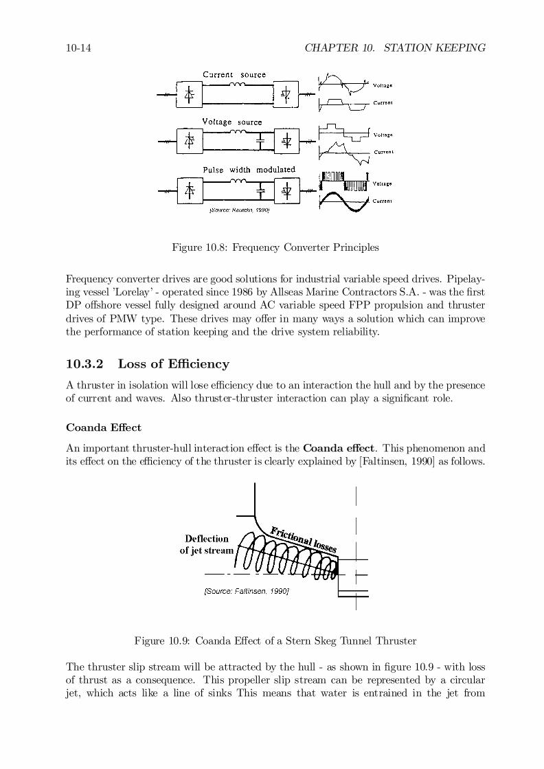
10-14 CHAPTER 10. STATION KEEPING
Figure 10.8: Frequency Converter Principles
Frequency converter drives are good solutions for industrial variable speed drives. Pipelay-ing vessel ’Lorelay’ - operated since 1986 by Allseas Marine Contractors S.A. - was the …rstDP o¤shore vessel fully designed around AC variable speed FPP propulsion and thrusterdrives of PMW type. These drives may o¤er in many ways a solution which can improvethe performance of station keeping and the drive system reliability.
10.3.2 Loss of E¢ciency
A thruster in isolation will lose e¢ciency due to an interaction the hull and by the presenceof current and waves. Also thruster-thruster interaction can play a signi…cant role.
Coanda E¤ect
An important thruster-hull interaction e¤ect is the Coanda e¤ect. This phenomenon andits e¤ect on the e¢ciency of the thruster is clearly explained by [Faltinsen, 1990] as follows.
Figure 10.9: Coanda E¤ect of a Stern Skeg Tunnel Thruster
The thruster slip stream will be attracted by the hull - as shown in …gure 10.9 - with lossof thrust as a consequence. This propeller slip stream can be represented by a circularjet, which acts like a line of sinks This means that water is entrained in the jet from
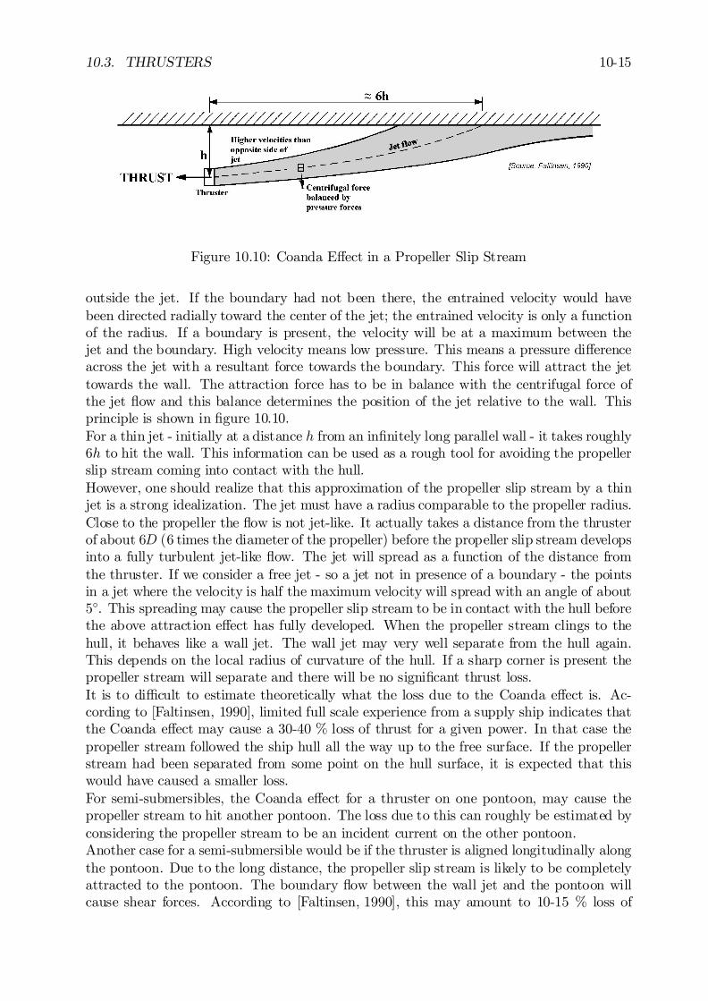
10.3. THRUSTERS 10-15
Figure 10.10: Coanda E¤ect in a Propeller Slip Stream
outside the jet. If the boundary had not been there, the entrained velocity would havebeen directed radially toward the center of the jet; the entrained velocity is only a functionof the radius. If a boundary is present, the velocity will be at a maximum between thejet and the boundary. High velocity means low pressure. This means a pressure di¤erenceacross the jet with a resultant force towards the boundary. This force will attract the jettowards the wall. The attraction force has to be in balance with the centrifugal force ofthe jet ‡ow and this balance determines the position of the jet relative to the wall. Thisprinciple is shown in …gure 10.10.For a thin jet - initially at a distance h from an in…nitely long parallel wall - it takes roughly6h to hit the wall. This information can be used as a rough tool for avoiding the propellerslip stream coming into contact with the hull.However, one should realize that this approximation of the propeller slip stream by a thinjet is a strong idealization. The jet must have a radius comparable to the propeller radius.Close to the propeller the ‡ow is not jet-like. It actually takes a distance from the thrusterof about 6D (6 times the diameter of the propeller) before the propeller slip stream developsinto a fully turbulent jet-like ‡ow. The jet will spread as a function of the distance fromthe thruster. If we consider a free jet - so a jet not in presence of a boundary - the pointsin a jet where the velocity is half the maximum velocity will spread with an angle of about5±. This spreading may cause the propeller slip stream to be in contact with the hull beforethe above attraction e¤ect has fully developed. When the propeller stream clings to thehull, it behaves like a wall jet. The wall jet may very well separate from the hull again.This depends on the local radius of curvature of the hull. If a sharp corner is present thepropeller stream will separate and there will be no signi…cant thrust loss.It is to di¢cult to estimate theoretically what the loss due to the Coanda e¤ect is. Ac-cording to [Faltinsen, 1990], limited full scale experience from a supply ship indicates thatthe Coanda e¤ect may cause a 30-40 % loss of thrust for a given power. In that case thepropeller stream followed the ship hull all the way up to the free surface. If the propellerstream had been separated from some point on the hull surface, it is expected that thiswould have caused a smaller loss.For semi-submersibles, the Coanda e¤ect for a thruster on one pontoon, may cause thepropeller stream to hit another pontoon. The loss due to this can roughly be estimated byconsidering the propeller stream to be an incident current on the other pontoon.Another case for a semi-submersible would be if the thruster is aligned longitudinally alongthe pontoon. Due to the long distance, the propeller slip stream is likely to be completelyattracted to the pontoon. The boundary ‡ow between the wall jet and the pontoon willcause shear forces. According to [Faltinsen, 1990], this may amount to 10-15 % loss of
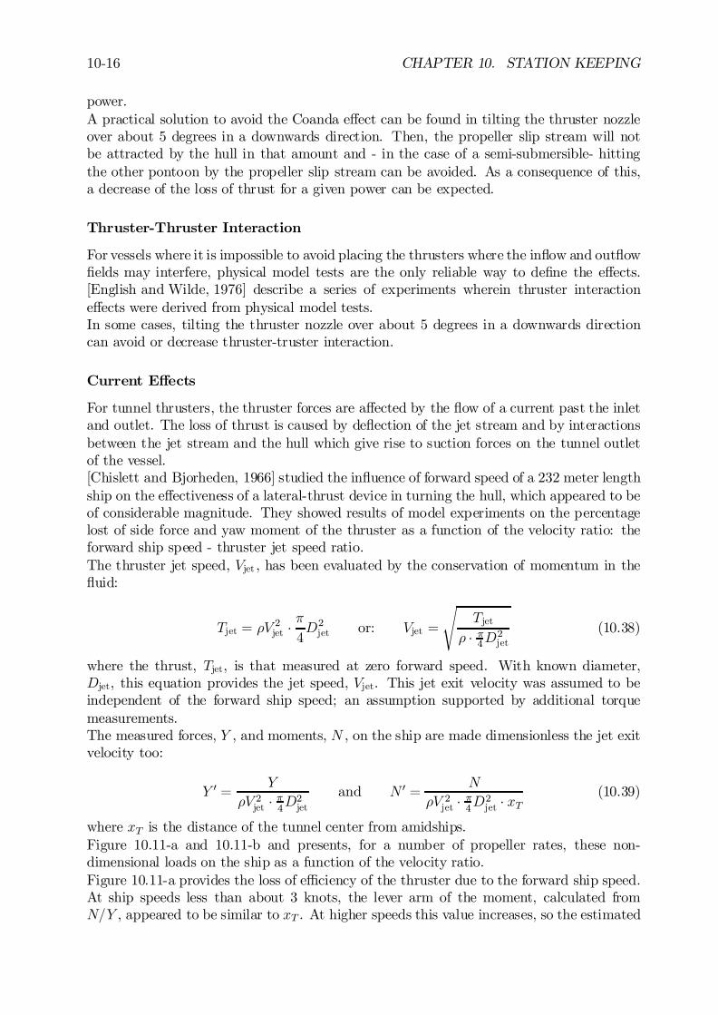
10-16 CHAPTER 10. STATION KEEPING
power.A practical solution to avoid the Coanda e¤ect can be found in tilting the thruster nozzleover about 5 degrees in a downwards direction. Then, the propeller slip stream will notbe attracted by the hull in that amount and - in the case of a semi-submersible- hittingthe other pontoon by the propeller slip stream can be avoided. As a consequence of this,a decrease of the loss of thrust for a given power can be expected.
Thruster-Thruster Interaction
For vessels where it is impossible to avoid placing the thrusters where the in‡ow and out‡ow…elds may interfere, physical model tests are the only reliable way to de…ne the e¤ects.[English and Wilde, 1976] describe a series of experiments wherein thruster interactione¤ects were derived from physical model tests.In some cases, tilting the thruster nozzle over about 5 degrees in a downwards directioncan avoid or decrease thruster-truster interaction.
Current E¤ects
For tunnel thrusters, the thruster forces are a¤ected by the ‡ow of a current past the inletand outlet. The loss of thrust is caused by de‡ection of the jet stream and by interactionsbetween the jet stream and the hull which give rise to suction forces on the tunnel outletof the vessel.[Chislett and Bjorheden, 1966] studied the in‡uence of forward speed of a 232 meter lengthship on the e¤ectiveness of a lateral-thrust device in turning the hull, which appeared to beof considerable magnitude. They showed results of model experiments on the percentagelost of side force and yaw moment of the thruster as a function of the velocity ratio: theforward ship speed - thruster jet speed ratio.The thruster jet speed, Vjet , has been evaluated by the conservation of momentum in the‡uid:
Tjet = ½V2jet ¢ ¼
4D2
jet or: Vjet =
sTjet
½ ¢ ¼4D2jet
(10.38)
where the thrust, Tjet, is that measured at zero forward speed. With known diameter,Djet, this equation provides the jet speed, Vjet. This jet exit velocity was assumed to beindependent of the forward ship speed; an assumption supported by additional torquemeasurements.The measured forces, Y , and moments, N , on the ship are made dimensionless the jet exitvelocity too:
Y 0 =Y
½V 2jet ¢ ¼4D2jet
and N 0 =N
½V 2jet ¢ ¼4D2
jet ¢ xT(10.39)
where xT is the distance of the tunnel center from amidships.Figure 10.11-a and 10.11-b and presents, for a number of propeller rates, these non-dimensional loads on the ship as a function of the velocity ratio.Figure 10.11-a provides the loss of e¢ciency of the thruster due to the forward ship speed.At ship speeds less than about 3 knots, the lever arm of the moment, calculated fromN=Y , appeared to be similar to xT . At higher speeds this value increases, so the estimated
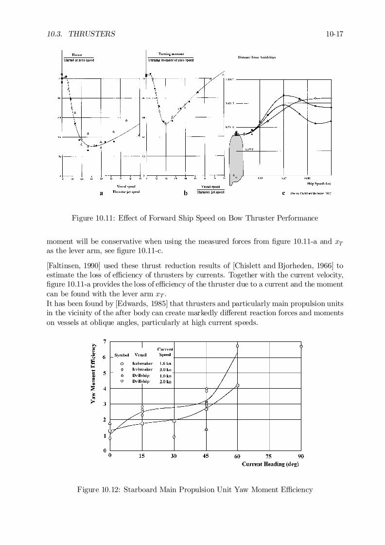
10.3. THRUSTERS 10-17
Figure 10.11: E¤ect of Forward Ship Speed on Bow Thruster Performance
moment will be conservative when using the measured forces from …gure 10.11-a and xTas the lever arm, see …gure 10.11-c.
[Faltinsen, 1990] used these thrust reduction results of [Chislett and Bjorheden, 1966] toestimate the loss of e¢ciency of thrusters by currents. Together with the current velocity,…gure 10.11-a provides the loss of e¢ciency of the thruster due to a current and the momentcan be found with the lever arm xT .It has been found by [Edwards, 1985] that thrusters and particularly main propulsion unitsin the vicinity of the after body can create markedly di¤erent reaction forces and momentson vessels at oblique angles, particularly at high current speeds.
Figure 10.12: Starboard Main Propulsion Unit Yaw Moment E¢ciency
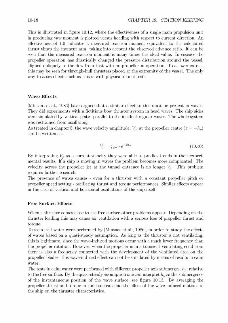
10-18 CHAPTER 10. STATION KEEPING
This is illustrated in …gure 10.12, where the e¤ectiveness of a single main propulsion unitin producing yaw moment is plotted versus heading with respect to current direction. Ane¤ectiveness of 1.0 indicates a measured reaction moment equivalent to the calculatedthrust times the moment arm, taking into account the observed advance ratio. It can beseen that the measured reaction moment is many times the ideal value. In essence thepropeller operation has drastically changed the pressure distribution around the vessel,aligned obliquely to the ‡ow from that with no propeller in operation. To a lower extent,this may be seen for through-hull thrusters placed at the extremity of the vessel. The onlyway to asses e¤ects such as this is with physical model tests.
Wave E¤ects
[Minsaas et al., 1986] have argued that a similar e¤ect to this must be present in waves.They did experiments with a …ctitious bow thruster system in head waves. The ship sideswere simulated by vertical plates parallel to the incident regular waves. The whole systemwas restrained from oscillating.As treated in chapter 5, the wave velocity amplitude, Vp, at the propeller centre (z = ¡hp)can be written as:
Vp = ³a! ¢ e¡khp (10.40)
By interpreting Vp as a current velocity they were able to predict trends in their experi-mental results. If a ship is moving in waves the problem becomes more complicated. Thevelocity across the propeller jet at the tunnel entrance is no longer Vp. This problemrequires further research.The presence of waves causes - even for a thruster with a constant propeller pitch orpropeller speed setting - oscillating thrust and torque performances. Similar e¤ects appearin the case of vertical and horizontal oscillations of the ship itself.
Free Surface E¤ects
When a thruster comes close to the free surface other problems appear. Depending on thethruster loading this may cause air ventilation with a serious loss of propeller thrust andtorque.Tests in still water were performed by [Minsaas et al., 1986], in order to study the e¤ectsof waves based on a quasi-steady assumption. As long as the thruster is not ventilating,this is legitimate, since the wave-induced motions occur with a much lower frequency thanthe propeller rotation. However, when the propeller is in a transient ventilating condition,there is also a frequency connected with the development of the ventilated area on thepropeller blades. this wave-induced e¤ect can not be simulated by means of results in calmwater.The tests in calm water were performed with di¤erent propeller axis submerges, hp, relativeto the free surface. By the quasi-steady assumption one can interpret hp as the submergenceof the instantaneous position of the wave surface, see …gure 10.13. By averaging thepropeller thrust and torque in time one can …nd the e¤ect of the wave induced motions ofthe ship on the thruster characteristics.
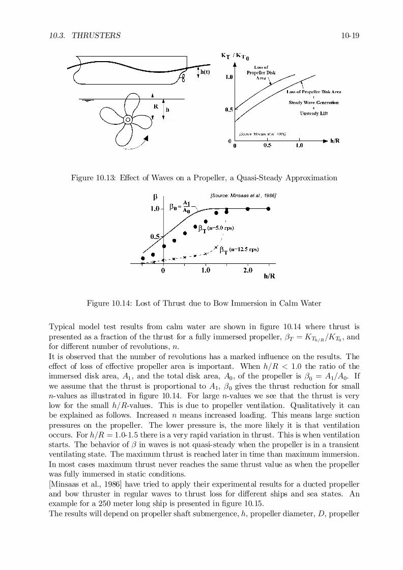
10.3. THRUSTERS 10-19
Figure 10.13: E¤ect of Waves on a Propeller, a Quasi-Steady Approximation
Figure 10.14: Lost of Thrust due to Bow Immersion in Calm Water
Typical model test results from calm water are shown in …gure 10.14 where thrust ispresented as a fraction of the thrust for a fully immersed propeller, ¯T =KTh=R=KT0 , andfor di¤erent number of revolutions, n.It is observed that the number of revolutions has a marked in‡uence on the results. Thee¤ect of loss of e¤ective propeller area is important. When h=R < 1:0 the ratio of theimmersed disk area, A1, and the total disk area, A0, of the propeller is ¯0 = A1=A0. Ifwe assume that the thrust is proportional to A1, ¯0 gives the thrust reduction for smalln-values as illustrated in …gure 10.14. For large n-values we see that the thrust is verylow for the small h=R-values. This is due to propeller ventilation. Qualitatively it canbe explained as follows. Increased n means increased loading. This means large suctionpressures on the propeller. The lower pressure is, the more likely it is that ventilationoccurs. For h=R = 1:0-1:5 there is a very rapid variation in thrust. This is when ventilationstarts. The behavior of ¯ in waves is not quasi-steady when the propeller is in a transientventilating state. The maximum thrust is reached later in time than maximum immersion.In most cases maximum thrust never reaches the same thrust value as when the propellerwas fully immersed in static conditions.[Minsaas et al., 1986] have tried to apply their experimental results for a ducted propellerand bow thruster in regular waves to thrust loss for di¤erent ships and sea states. Anexample for a 250 meter long ship is presented in …gure 10.15.The results will depend on propeller shaft submergence, h, propeller diameter, D, propeller
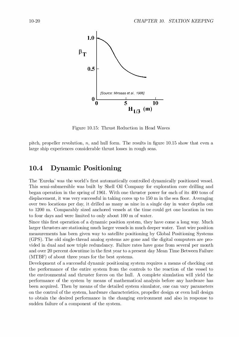
10-20 CHAPTER 10. STATION KEEPING
Figure 10.15: Thrust Reduction in Head Waves
pitch, propeller revolution, n, and hull form. The results in …gure 10.15 show that even alarge ship experiences considerable thrust losses in rough seas.
10.4 Dynamic Positioning
The ’Eureka’ was the world’s …rst automatically controlled dynamically positioned vessel.This semi-submersible was built by Shell Oil Company for exploration core drilling andbegan operation in the spring of 1961. With one thruster power for each of its 400 tons ofdisplacement, it was very successful in taking cores up to 150 m in the sea ‡oor. Averagingover two locations per day, it drilled as many as nine in a single day in water depths outto 1200 m. Comparably sized anchored vessels at the time could get one location in twoto four days and were limited to only about 100 m of water.Since this …rst operation of a dynamic position system, they have come a long way. Muchlarger thrusters are stationing much larger vessels in much deeper water. Taut wire positionmeasurements has been given way to satellite positioning by Global Positioning Systems(GPS). The old single-thread analog systems are gone and the digital computers are pro-vided in dual and now triple redundancy. Failure rates have gone from several per monthand over 20 percent downtime in the …rst year to a present day Mean Time Between Failure(MTBF) of about three years for the best systems.Development of a successful dynamic positioning system requires a means of checking outthe performance of the entire system from the controls to the reaction of the vessel tothe environmental and thruster forces on the hull. A complete simulation will yield theperformance of the system by means of mathematical analysis before any hardware hasbeen acquired. Then by means of the detailed system simulator, one can vary parameterson the control of the system, hardware characteristics, propeller design or even hull designto obtain the desired performance in the changing environment and also in response tosudden failure of a component of the system.
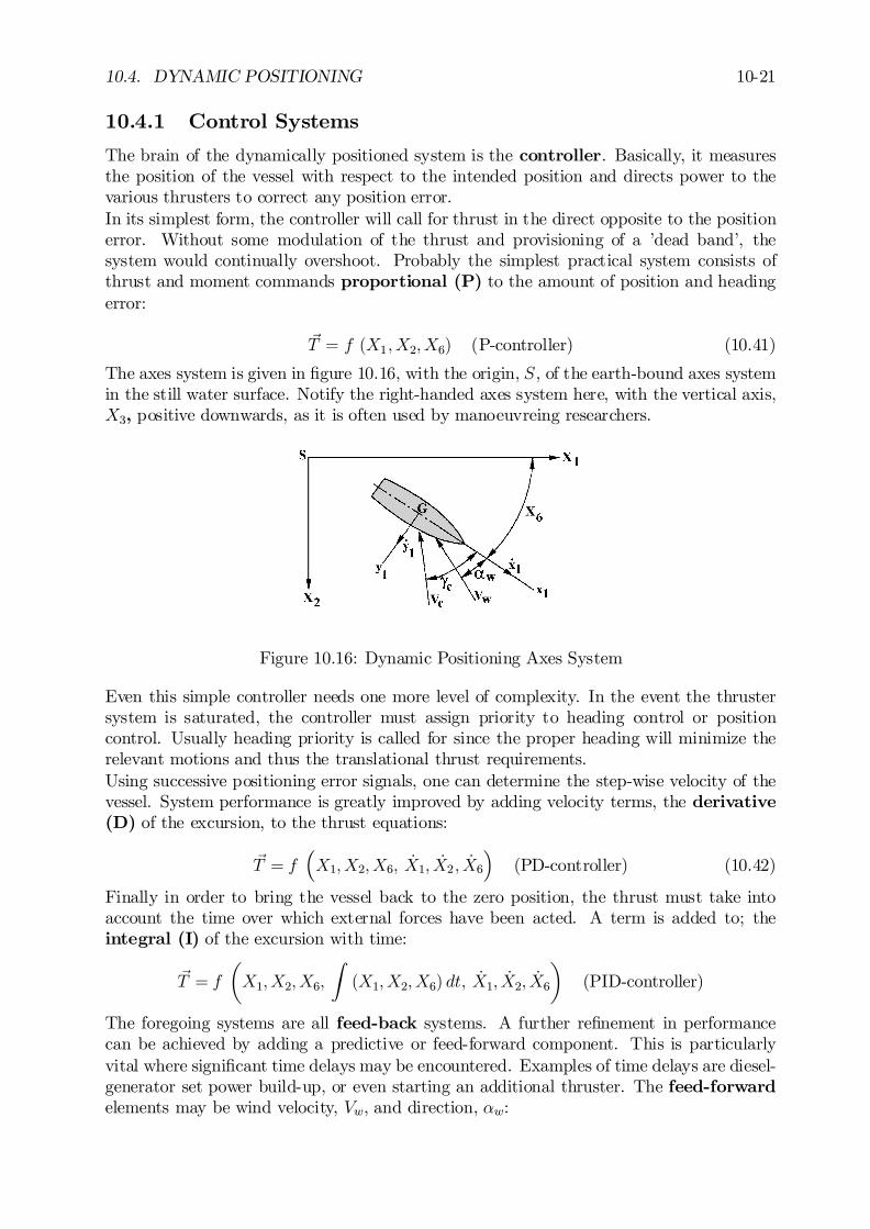
10.4. DYNAMIC POSITIONING 10-21
10.4.1 Control Systems
The brain of the dynamically positioned system is the controller. Basically, it measuresthe position of the vessel with respect to the intended position and directs power to thevarious thrusters to correct any position error.In its simplest form, the controller will call for thrust in the direct opposite to the positionerror. Without some modulation of the thrust and provisioning of a ’dead band’, thesystem would continually overshoot. Probably the simplest practical system consists ofthrust and moment commands proportional (P) to the amount of position and headingerror:
~T = f (X1; X2; X6) (P-controller) (10.41)
The axes system is given in …gure 10.16, with the origin, S , of the earth-bound axes systemin the still water surface. Notify the right-handed axes system here, with the vertical axis,X3, positive downwards, as it is often used by manoeuvreing researchers.
Figure 10.16: Dynamic Positioning Axes System
Even this simple controller needs one more level of complexity. In the event the thrustersystem is saturated, the controller must assign priority to heading control or positioncontrol. Usually heading priority is called for since the proper heading will minimize therelevant motions and thus the translational thrust requirements.Using successive positioning error signals, one can determine the step-wise velocity of thevessel. System performance is greatly improved by adding velocity terms, the derivative(D) of the excursion, to the thrust equations:
~T = f³X1; X2; X6; _X1; _X2; _X6
´(PD-controller) (10.42)
Finally in order to bring the vessel back to the zero position, the thrust must take intoaccount the time over which external forces have been acted. A term is added to; theintegral (I) of the excursion with time:
~T = f
µX1; X2; X6;
Z(X1; X2; X6) dt; _X1; _X2; _X6
¶(PID-controller)
The foregoing systems are all feed-back systems. A further re…nement in performancecan be achieved by adding a predictive or feed-forward component. This is particularlyvital where signi…cant time delays may be encountered. Examples of time delays are diesel-generator set power build-up, or even starting an additional thruster. The feed-forwardelements may be wind velocity, Vw, and direction, ®w:
10-22 CHAPTER 10. STATION KEEPING
(PID-controller with
~T = f
µX1; X2; X6;
Z(X1; X2; X6) dt; _X1; _X2; _X6; Vw; ®w
¶wind-feed-forward)
(10.43)
[Pinkster, 1978] suggested to extend the wind-feed-forward system with an intriguing wave-feed-forward system. He carried out model experiments in bow-quartering irregular waves(H1=3 = 4:9 m and T2 = 10:2 s) and a stern-quartering current (1 knot). The wave-feed-forward system consisted of 8 ship-mounted wave probes. He showed that a wave-feed-forward system is capable to reduce the low-frequency part of the sway motion by about70 % and the surge motion by about 50 %. The DP simulation procedure can be extendedto include this factor, but the value of the simulation would depend primarily on the degreeto which the simulated wave data represents possible actual wave measurements. So far,wave-feed-forward has not yet been incorporated in DP simulations.
The possibilities for evaluating the generalized function of eleven variables in equation10.43 are limitless, hence the need for mathematical simulation.
10.4.2 Mathematical Model
For a dynamically positioned ‡oating structure, only the horizontal low-frequency motionsfor surge (k = 1), sway (k = 2) and yaw (k = 6) are of interest. The thruster forces haveto balance the mean wave, current and wind loads. Further, Äxk, _xk and xk are the slowlyvarying motions of the structure. It are the high-frequency motions of the waves that areneglected or …ltered out, because it is generally impossible to have a system that can reactto these high-frequency wave forces.
A general form of the three nonlinear coupled (Euler) equations of motion in the horizontalplane for surge, sway and yaw of a DP vessel - with an axes system as given in …gure 10.16- is given by:
(½r + a11) ¢ Äx1 (t) + b11 ¢ _x1 (t) + bV1 ¢ _x1 (t) ¢ j _x1 (t)j ¡ (½r + a22) ¢ _x2 (t) ¢ _x6 (t) == FW1 (t) +F
C1 (t) + F
WD1 (t) +F R1 (t) + T1 (t)
(½r + a22) ¢ Äx2 (t) + b22 ¢ _x2 (t) + bV2 ¢ _x2 (t) ¢ j _x2 (t)j+ (½r + a11) ¢ _x1 (t) ¢ _x6 (t) == FW2 (t) +F
C2 (t) + F
WD2 (t) +F R2 (t) + T2 (t)
(I66 + a66) ¢ Äx6 (t) + b66 ¢ _x6 (t) + bV6 ¢ _x6 (t) ¢ j _x6 (t)j ¡ (a11 ¡ a22) ¢ _x1 (t) ¢ _x2 (t) == FW6 (t) +F
C6 (t) + F
WD6 (t) +F R6 (t) + T6 (t)
(10.44)
where ½r is the solid mass of the ship, I66 is the mass moment of inertia of the ship, akkis the hydrodynamic mass or inertia, bkk is the hydrodynamic damping coe¢cient, bVk isthe quadratic viscous drag force or moment coe¢cient, FWk is the wind force or moment,FCk is the current force or moment FWDk is the slow-drift wave excitation force or moment,FRk (t) is the force or moment due to the riser and Tk is the thruster force or moment.
10.4. DYNAMIC POSITIONING 10-23
Notice the appearance here of a sway-yaw velocity coupling term in the surge equation, asurge-yaw velocity coupling term in the sway equation and a surge-sway velocity couplingterm in the yaw equation. These three mass terms follow from a proper derivation ofthe nonlinear Euler equations of motion in the horizontal plane, which has been treatedplentiful in the literature on manoeuvering, guidance and control of ships; for instance[Fossen, 1994].
The relative water velocity and direction - see …gure 10.16 - are:
VCR =
q( _x1+ VC cos °C)
2 + ( _x2 + VC sin°C)2
°CR = arctan
µ_x2 + VC sin°C_x1 + VC cos °C
¶(10.45)
Then the current forces and moments can be obtained by:
FCk = R0k
¡°CR
¢¢ V 2CR for : k = 1; 2; 6 (10.46)
where R0k¡°CR
¢is the resistance coe¢cient in the xk-direction due to the relative water
velocity in the °CR-direction.The vessel velocities along the …xed (global) axes (X1; X2) are related to the velocitiesalong the local axes by the following transformation relations:
_X1 = _x1 cos x6 ¡ _x2 sinx6_X2 = _x2 sinx6 + _x2 cos x6_X6 = _x6 (10.47)
In addition, the excursions in surge sway and yaw are obtained from:
X1 =
Z_X1 ¢ dt X2 =
Z_X2 ¢ dt X6 =
Z_X6 ¢ dt (10.48)
The …rst-order di¤erential equations governing thrust build-up with time of a DP systemwith a PID-controller can be written in the form:
T1+ ¿ 1 ¢ dT1dt
= ¡KP1 ¢X1 ¡K I
1 ¢tZ
0
X1 ¢ dt¡KD1 ¢ _X1
T2+ ¿ 2 ¢ dT2dt
= ¡KP2 ¢X2 ¡K I
2 ¢tZ
0
X2 ¢ dt¡KD2 ¢ _X2
T6+ ¿ 6 ¢ dT6dt
= ¡KP6 ¢X6 ¡K I
6 ¢tZ
0
X6 ¢ dt¡KD6 ¢ _X6 (10.49)
where ¿k are time constants and the right hand term and KPk , K I
kand KDk are gain
constants of the PID-controller.Sometimes, a low-pass …lter is used in the last term, KD
i ¢ _Xi, which avoids undesirablee¤ects of high frequencies.
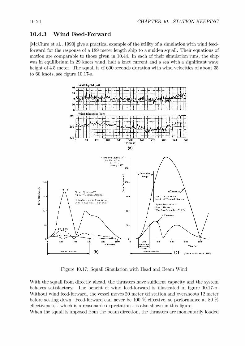
10-24 CHAPTER 10. STATION KEEPING
10.4.3 Wind Feed-Forward
[McClure et al., 1990] give a practical example of the utility of a simulation with wind feed-forward for the response of a 189 meter length ship to a sudden squall. Their equations ofmotion are comparable to those given in 10.44. In each of their simulation runs, the shipwas in equilibrium in 29 knots wind, half a knot current and a sea with a signi…cant waveheight of 4.5 meter. The squall is of 600 seconds duration with wind velocities of about 35to 60 knots, see …gure 10.17-a.
Figure 10.17: Squall Simulation with Head and Beam Wind
With the squall from directly ahead, the thrusters have su¢cient capacity and the systembehaves satisfactory. The bene…t of wind feed-forward is illustrated in …gure 10.17-b.Without wind feed-forward, the vessel moves 20 meter o¤ station and overshoots 12 meterbefore setting down. Feed-forward can never be 100 % e¤ective, so performance at 80 %e¤ectiveness - which is a reasonable expectation - is also shown in this …gure.When the squall is imposed from the beam direction, the thrusters are momentarily loaded
10.4. DYNAMIC POSITIONING 10-25
to capacity and the system is ’saturated’. Figure 10.17-c illustrates the necessity of pro-viding thrust in excess of the static balance. The curves shown represent in one case 3thrusters available, 10,300 kWh, and in the other case 6 thrusters totalling 7725 kWh.Either system has more than enough thrust to exceed the equilibrium loading. Both casesinclude wind feed-forward at 80 % e¤ectiveness. Note that the time during which thesystem is saturated is relatively brief, yet the system allows large drift and overshoot.
10.4.4 Gain Constants Estimate
For a DP system there has to be an allocation system that tells how the power should bedistributed among the individual thruster units. If the thrusters are a part of a DP systemwith a PD-controller, an idealized simpli…cation of the total thruster forces - with timeconstant ¿ ! 0 - can be written as:
Tk = ¡KPk ¢Xk ¡KD
k ¢ _Xk for: k = 1; 2; 6 (10.50)
[Faltinsen, 1990] proposes a simple method to get a feeling for the magnitude of the gainconstants, KD
k and KPk of the PD-controller of a dynamically positioned ship. An example
is given here for surge, of which the simpli…ed uncoupled equation of the slow-drift motionis given by:
(m11 + a11) ¢ Äx1 + b11 ¢ _x1 = FSW1 + FW1 + T1 (10.51)
A substitution of equation 10.50 (with x1 = X1 and _x1 = _X1) in equation 10.51 providesequation 10.52 for surge of the DP vessel:
(m11 + a11) ¢ Äx1 +¡b11 +K
D1
¢¢ _x1 +KP
1 ¢ x1 = F SW1 +FW1 (10.52)
where m11 is the mass of the ship, a11 is the hydrodynamic mass, b11 is the hydrodynamicdamping, F SW1 is the slow-drift wave excitation force and FW1 the gust force. The meanvalues of F SW1 and FW1 are supposed to be zero.The gain constant KP
1 will be chosen so that the natural period in surge of the slowlyoscillating ship is from 100-200 seconds. The damping coe¢cient, b11, has been neglectedby Faltinsen at this very low frequency and the gain constant KD
1 was set equal to about60 % of the critical damping; so · = 0:60, see chapter 6. The …nal real values will bedecided after full scale sea tests with the DP system.Thus, as a …rst estimate:
KP1 = !20 ¢ (m11 + a11) where !0 =
150
2¼, for instance
KD1 = 1:20 ¢
q(m11 + a11) ¢KP
1 (10.53)
With these equations, the variance of the slow-drift surge motion can be calculated in away as has been done in chapter 6 for motions with frequencies in the wave-frequencyrange. Finally, the variance of the total thruster forces follow from equation 10.50.For ships, the potential mass for surge can be approximated by 5-8 % of the ship’s solidmass. The damping coe¢cient, b11, has assumed to be zero here. This assumption is truefor the potential damping but viscous e¤ects can have some in‡uence. In some papers, theuse of a surge damping coe¢cient of about 5 % of the critical damping of a soft springsystem is recommended.

10-26 CHAPTER 10. STATION KEEPING
10.4.5 Motion Reference Filtering
Suppose a simple uncoupled equation of motion for sway of a DP vessel, given by:
(m22 + a22) ¢ Äx2 (t) + b22 ¢ _x2 (t) = FD2 (t) + T2 (t) (10.54)
where FD2 (t) is the total sway drift force and T2 (t) is the total sway thruster force.The use of a PD-controller means that the thruster force contains a part which is propor-tional (P) to the position error, x2 (t), and a part which is proportional to the derivative(D) to time of this position error, the velocity _x2 (t). To obtain ’smooth’ input signalsx2 (t) and _x2 (t), the measured reference signal, x2 (t) - being obtained by systems suchas Loran, GPS, a taut wire system or an acoustic system - has to be …ltered; the wavefrequency motions and the high frequency disturbances are …ltered out. But, …ltering - forinstance by using a Kalman …lter - necessarily introduces a time lag, ¿ . Due to this timelag, the thruster force is applied ’later’:
T2 (t) = ¡KP2 ¢X (t ¡ ¿ ) ¡KD
2 ¢ _X2 (t¡ ¿) (10.55)
where ¿ is the time lag of the DP system between the …ltered motion signals and thethruster reaction.However, thruster forces are a¤ected by the presence of waves. This holds that - in spiteof …ltering out of wave frequent motions - via the actual thruster forces wave frequentcontributions will be introduced again in the system.The displacement and velocity can be expanded in series:
X2 (t¡ ¿) = X2 (t)¡@ fX2 (t)g
@t¢ ¿ + ::::::
_X2 (t¡ ¿) = _X2 (t)¡@
n_X2 (t)
o
@t¢ ¿ + :::::: (10.56)
These series can be simpli…ed by assuming ¿ to be small relative to the natural period ofthe sway motion; thus a linearization is permitted:
X2 (t ¡ ¿) = X2 (t)¡ _X2 (t) ¢ ¿_X2 (t ¡ ¿) = _X2 (t)¡ ÄX2 (t) ¢ ¿ (10.57)
so:T2 (t) = +K
D2 ¢ ÄX2 (t) ¢ ¿ +
©¡KD
2 +KP2 ¢ ¿
ª¢ _X2 (t) ¡KP
2 ¢X2 (t) (10.58)
With Äx2 = ÄX2, _x2 = _X2 and x2 = X2, the following expression is found from equation10.54:¡m22+ a22 ¡KD
2 ¢ ¿¢
¢ Äx2 (t) +¡b22 +K
D2 ¡KP
2 ¢ ¿¢
¢ _x2 (t) +KP2 ¢ x2 (t) = FD2 (t) (10.59)
This equation shows that the e¤ect of a time lag in the DP system is to reduce the massterm in the equation of motion and also to reduce the damping term.Assuming that the total sway drift force, FD2 (t), can be characterized as a low frequency’white noise’ process with mean value FD2 and the spectral density, Sf , the above equation
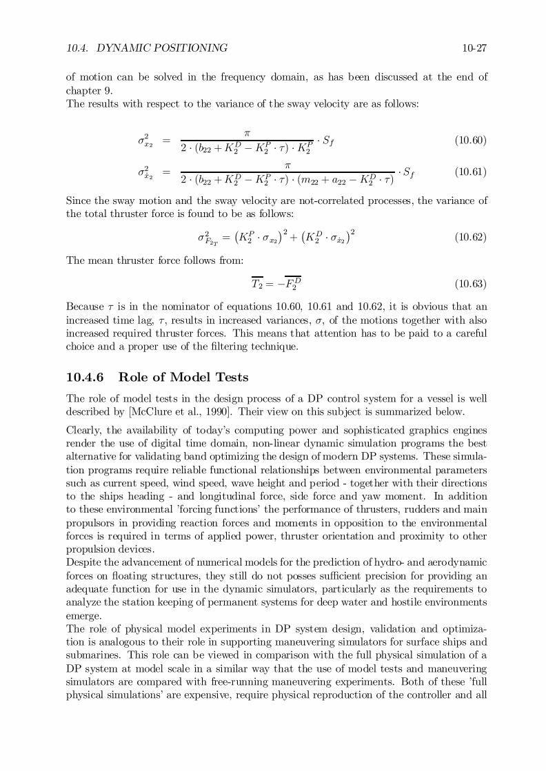
10.4. DYNAMIC POSITIONING 10-27
of motion can be solved in the frequency domain, as has been discussed at the end ofchapter 9.The results with respect to the variance of the sway velocity are as follows:
¾2x2 =¼
2 ¢ (b22 +KD2 ¡KP
2 ¢ ¿) ¢KP2
¢ Sf (10.60)
¾2_x2 =¼
2 ¢ (b22 +KD2 ¡KP
2 ¢ ¿) ¢ (m22 + a22 ¡KD2 ¢ ¿) ¢Sf (10.61)
Since the sway motion and the sway velocity are not-correlated processes, the variance ofthe total thruster force is found to be as follows:
¾2F2T =¡KP2 ¢ ¾x2
¢2+
¡KD2 ¢ ¾ _x2
¢2 (10.62)
The mean thruster force follows from:
T2 = ¡FD2 (10.63)
Because ¿ is in the nominator of equations 10.60, 10.61 and 10.62, it is obvious that anincreased time lag, ¿, results in increased variances, ¾, of the motions together with alsoincreased required thruster forces. This means that attention has to be paid to a carefulchoice and a proper use of the …ltering technique.
10.4.6 Role of Model Tests
The role of model tests in the design process of a DP control system for a vessel is welldescribed by [McClure et al., 1990]. Their view on this subject is summarized below.
Clearly, the availability of today’s computing power and sophisticated graphics enginesrender the use of digital time domain, non-linear dynamic simulation programs the bestalternative for validating band optimizing the design of modern DP systems. These simula-tion programs require reliable functional relationships between environmental parameterssuch as current speed, wind speed, wave height and period - together with their directionsto the ships heading - and longitudinal force, side force and yaw moment. In additionto these environmental ’forcing functions’ the performance of thrusters, rudders and mainpropulsors in providing reaction forces and moments in opposition to the environmentalforces is required in terms of applied power, thruster orientation and proximity to otherpropulsion devices.Despite the advancement of numerical models for the prediction of hydro- and aerodynamicforces on ‡oating structures, they still do not posses su¢cient precision for providing anadequate function for use in the dynamic simulators, particularly as the requirements toanalyze the station keeping of permanent systems for deep water and hostile environmentsemerge.The role of physical model experiments in DP system design, validation and optimiza-tion is analogous to their role in supporting maneuvering simulators for surface ships andsubmarines. This role can be viewed in comparison with the full physical simulation of aDP system at model scale in a similar way that the use of model tests and maneuveringsimulators are compared with free-running maneuvering experiments. Both of these ’fullphysical simulations’ are expensive, require physical reproduction of the controller and all
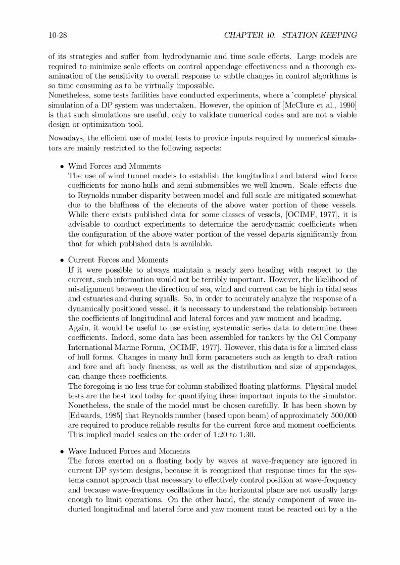
10-28 CHAPTER 10. STATION KEEPING
of its strategies and su¤er from hydrodynamic and time scale e¤ects. Large models arerequired to minimize scale e¤ects on control appendage e¤ectiveness and a thorough ex-amination of the sensitivity to overall response to subtle changes in control algorithms isso time consuming as to be virtually impossible.Nonetheless, some tests facilities have conducted experiments, where a ’complete’ physicalsimulation of a DP system was undertaken. However, the opinion of [McClure et al., 1990]is that such simulations are useful, only to validate numerical codes and are not a viabledesign or optimization tool.
Nowadays, the e¢cient use of model tests to provide inputs required by numerical simula-tors are mainly restricted to the following aspects:
² Wind Forces and MomentsThe use of wind tunnel models to establish the longitudinal and lateral wind forcecoe¢cients for mono-hulls and semi-submersibles we well-known. Scale e¤ects dueto Reynolds number disparity between model and full scale are mitigated somewhatdue to the blu¤ness of the elements of the above water portion of these vessels.While there exists published data for some classes of vessels, [OCIMF, 1977], it isadvisable to conduct experiments to determine the aerodynamic coe¢cients whenthe con…guration of the above water portion of the vessel departs signi…cantly fromthat for which published data is available.
² Current Forces and MomentsIf it were possible to always maintain a nearly zero heading with respect to thecurrent, such information would not be terribly important. However, the likelihood ofmisalignment between the direction of sea, wind and current can be high in tidal seasand estuaries and during squalls. So, in order to accurately analyze the response of adynamically positioned vessel, it is necessary to understand the relationship betweenthe coe¢cients of longitudinal and lateral forces and yaw moment and heading.Again, it would be useful to use existing systematic series data to determine thesecoe¢cients. Indeed, some data has been assembled for tankers by the Oil CompanyInternational Marine Forum, [OCIMF, 1977]. However, this data is for a limited classof hull forms. Changes in many hull form parameters such as length to draft rationand fore and aft body …neness, as well as the distribution and size of appendages,can change these coe¢cients.The foregoing is no less true for column stabilized ‡oating platforms. Physical modeltests are the best tool today for quantifying these important inputs to the simulator.Nonetheless, the scale of the model must be chosen carefully. It has been shown by[Edwards, 1985] that Reynolds number (based upon beam) of approximately 500,000are required to produce reliable results for the current force and moment coe¢cients.This implied model scales on the order of 1:20 to 1:30.
² Wave Induced Forces and MomentsThe forces exerted on a ‡oating body by waves at wave-frequency are ignored incurrent DP system designs, because it is recognized that response times for the sys-tems cannot approach that necessary to e¤ectively control position at wave-frequencyand because wave-frequency oscillations in the horizontal plane are not usually largeenough to limit operations. On the other hand, the steady component of wave in-ducted longitudinal and lateral force and yaw moment must be reacted out by a the

10.4. DYNAMIC POSITIONING 10-29
positioning system. The slowly varying component of these forces and moments mustbe at least be attenuated.Numerical models have been developed which provide estimates of the steady andslowly varying components of the wave drift forces and moments. Nonetheless, tocon…rm these estimates for new designs, it is advisable to obtain a semi-empiricalrelationship between the steady force and moment coe¢cients and wave period inregular waves. Estimates of the slowly varying drift force and moment coe¢cientscan also be derived from experiments in regular wave ’beats’ and from irregular wavetests using cross bi-spectral analysis techniques to derive quadratic transfer functionsfor second order wave forces. These model tests can be conducted using relative smalland inexpensive models, on the order of 1:50, because viscous e¤ects are relativelyunimportant in physical simulation of wave drift.
² Thruster E¤ectivenessThe e¤ectiveness of thrusters in producing forces and moments to react out theenvironmental forces and moments is necessary information for the simulator. It isnot adequate to consider the thruster in isolation, as done in a foregoing section,because depending upon the proximity of thrusters, their in‡ow and out‡ow …eldscan interact, producing deviations in e¤ectiveness from that which would be expectedif the thrusters’ force and moment applied to the vessel were calculated taking in‡owvelocity (free stream current), propeller angular speed and pitch into account andusing performance curves for the isolated thruster. For vessels where it is impossibleto avoid placing the thrusters where the in‡ow and out‡ow …elds may interfere,physical model tests are the only reliable way to de…ne the e¤ects.These experiments are carried out best with a large captive model. The modelis restrained in surge, sway and yaw. The model is towed at various speeds andheadings and various thruster operating conditions are prescribed. The resultingresidual forces and moments are measured. This data base is used in conjunction witha similar data base obtained from towed tests without the thrusters and propulsorsoperating to derive the e¤ectiveness and interaction polar plots for the thrusters andpropulsors.

10-30 CHAPTER 10. STATION KEEPING
.
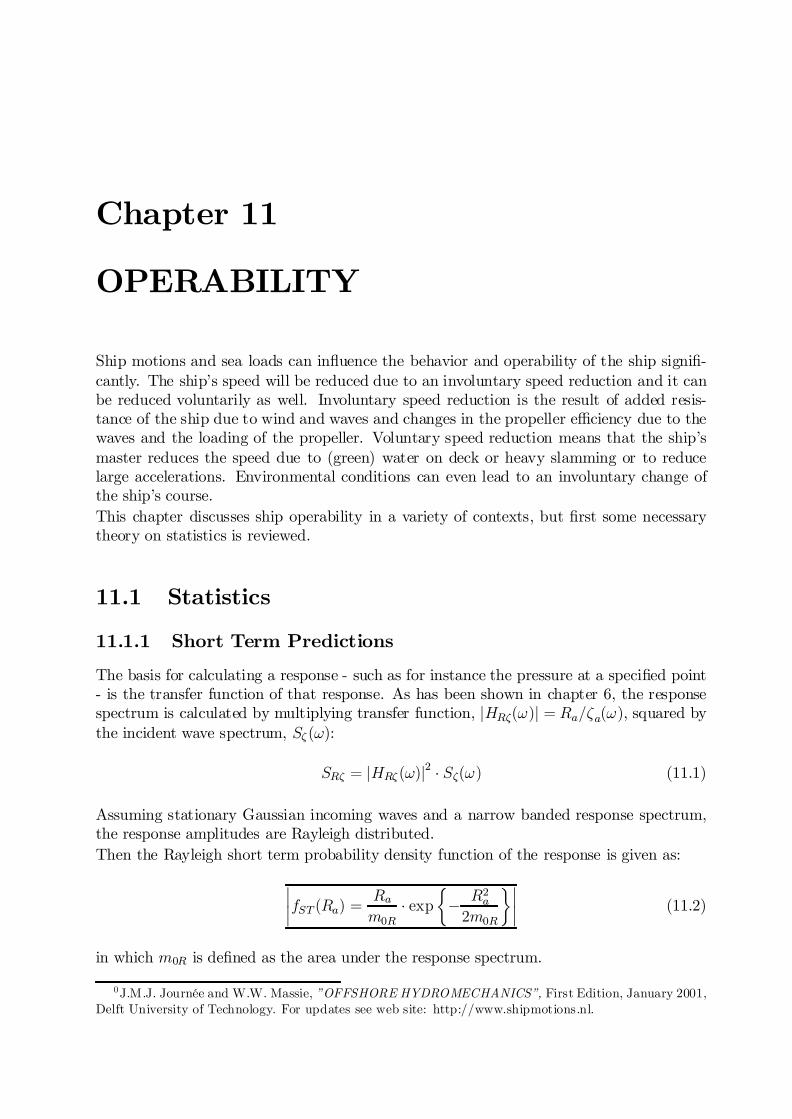
Chapter 11
OPERABILITY
Ship motions and sea loads can in‡uence the behavior and operability of the ship signi…-cantly. The ship’s speed will be reduced due to an involuntary speed reduction and it canbe reduced voluntarily as well. Involuntary speed reduction is the result of added resis-tance of the ship due to wind and waves and changes in the propeller e¢ciency due to thewaves and the loading of the propeller. Voluntary speed reduction means that the ship’smaster reduces the speed due to (green) water on deck or heavy slamming or to reducelarge accelerations. Environmental conditions can even lead to an involuntary change ofthe ship’s course.This chapter discusses ship operability in a variety of contexts, but …rst some necessarytheory on statistics is reviewed.
11.1 Statistics
11.1.1 Short Term Predictions
The basis for calculating a response - such as for instance the pressure at a speci…ed point- is the transfer function of that response. As has been shown in chapter 6, the responsespectrum is calculated by multiplying transfer function, jHR³(!)j = Ra=³a(!), squared bythe incident wave spectrum, S³ (!):
SR³ = jHR³ (!)j2 ¢ S³(!) (11.1)
Assuming stationary Gaussian incoming waves and a narrow banded response spectrum,the response amplitudes are Rayleigh distributed.Then the Rayleigh short term probability density function of the response is given as:
¯¯fST (Ra) =
Ram0R
¢ exp½
¡ R2a2m0R
¾¯¯ (11.2)
in which m0R is de…ned as the area under the response spectrum.
0J.M.J. Journée and W.W. Massie, ”OFFSHORE HYDROMECHANICS”, First Edition, January 2001,Delft University of Technology. For updates see web site: http://www.shipmotions.nl.
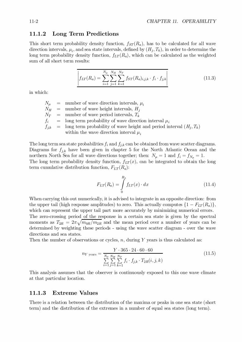
11-2 CHAPTER 11. OPERABILITY
11.1.2 Long Term Predictions
This short term probability density function, fST (Ra), has to be calculated for all wavedirection intervals, ¹i, and sea state intervals, de…ned by (Hj; Tk), in order to determine thelong term probability density function, fLT (Ra), which can be calculated as the weightedsum of all short term results:
¯¯¯fLT (Ra) =
N¹X
i=1
NHX
j=1
NTX
k=1
fST (Ra)i;j;k ¢ fi ¢ fj;k¯¯¯ (11.3)
in which:
N¹ = number of wave direction intervals, ¹iNH = number of wave height intervals, HjNT = number of wave period intervals, Tkfi = long term probability of wave direction interval ¹ifj;k = long term probability of wave height and period interval (Hj; Tk)
within the wave direction interval ¹i
The long term sea state probabilities fi and fj;k can be obtained from wave scatter diagrams.Diagrams for fj;k have been given in chapter 5 for the North Atlantic Ocean and thenorthern North Sea for all wave directions together; then: N¹ = 1 and fi = fN¹ = 1.The long term probability density function, fLT (x), can be integrated to obtain the longterm cumulative distribution function, FLT (Ra):
FLT(Ra) =
RaZ
0
fLT (x) ¢ dx (11.4)
When carrying this out numerically, it is advised to integrate in an opposite direction: fromthe upper tail (high response amplitudes) to zero. This actually computes f1 ¡ FLT (Ra)g,which can represent the upper tail part more accurately by minimizing numerical errors.The zero-crossing period of the response in a certain sea state is given by the spectralmoments as T2R = 2¼
pm0R=m2R and the mean period over a number of years can be
determined by weighting these periods - using the wave scatter diagram - over the wavedirections and sea states.Then the number of observations or cycles, n, during Y years is thus calculated as:
nY years =Y ¢ 365 ¢ 24 ¢ 60 ¢ 60
N¹Pi=1
NHPj=1
NTPk=1
fi ¢ fj;k ¢ T2R(i; j; k)(11.5)
This analysis assumes that the observer is continuously exposed to this one wave climateat that particular location.
11.1.3 Extreme Values
There is a relation between the distribution of the maxima or peaks in one sea state (shortterm) and the distribution of the extremes in a number of equal sea states (long term).
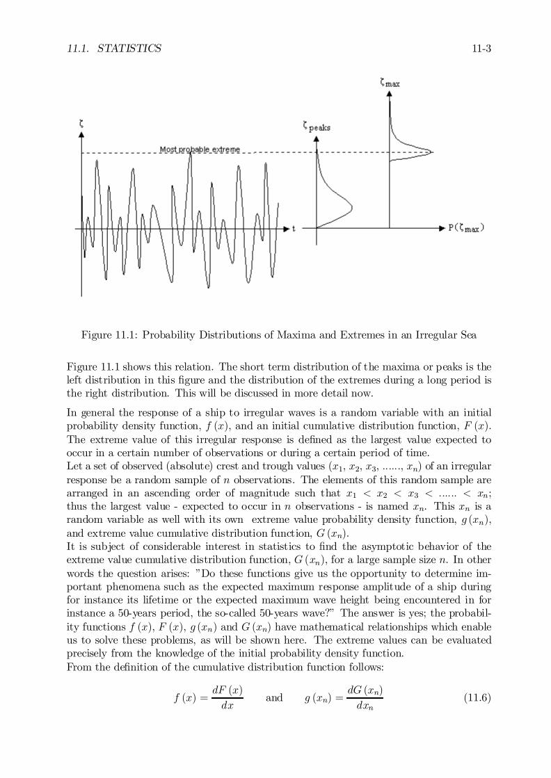
11.1. STATISTICS 11-3
Figure 11.1: Probability Distributions of Maxima and Extremes in an Irregular Sea
Figure 11.1 shows this relation. The short term distribution of the maxima or peaks is theleft distribution in this …gure and the distribution of the extremes during a long period isthe right distribution. This will be discussed in more detail now.
In general the response of a ship to irregular waves is a random variable with an initialprobability density function, f (x), and an initial cumulative distribution function, F (x).The extreme value of this irregular response is de…ned as the largest value expected tooccur in a certain number of observations or during a certain period of time.Let a set of observed (absolute) crest and trough values (x1, x2, x3, ::::::, xn) of an irregularresponse be a random sample of n observations. The elements of this random sample arearranged in an ascending order of magnitude such that x1 < x2 < x3 < :::::: < xn;thus the largest value - expected to occur in n observations - is named xn. This xn is arandom variable as well with its own extreme value probability density function, g (xn),and extreme value cumulative distribution function, G (xn).It is subject of considerable interest in statistics to …nd the asymptotic behavior of theextreme value cumulative distribution function, G (xn), for a large sample size n. In otherwords the question arises: ”Do these functions give us the opportunity to determine im-portant phenomena such as the expected maximum response amplitude of a ship duringfor instance its lifetime or the expected maximum wave height being encountered in forinstance a 50-years period, the so-called 50-years wave?” The answer is yes; the probabil-ity functions f (x), F (x), g (xn) and G (xn) have mathematical relationships which enableus to solve these problems, as will be shown here. The extreme values can be evaluatedprecisely from the knowledge of the initial probability density function.From the de…nition of the cumulative distribution function follows:
f (x) =dF (x)
dxand g (xn) =
dG (xn)
dxn(11.6)

11-4 CHAPTER 11. OPERABILITY
As has been shown in chapter 5 for irregular waves, the probability that an arbitraryresponse amplitude in irregular waves, Ra, does not exceed a value A is given by:
P fRa < Ag =AZ
0
f (x) ¢ dx = F (A) (11.7)
Thus, the probability that one response amplitude in irregular waves does not exceed avalue xn is given by:
P fx < xng in 1 observation = F (xn) (11.8)
The probability that n response amplitudes in irregular waves does not exceed a value xnfollows from a multiplication of the individual probabilities - assuming independence of theindividual response amplitudes - by:
P fx < xng in n observations = (P fx < xng)n
= fF (xn)gn (11.9)
Thus, the extreme value cumulative distribution function, G (xn), in n observations can beformulated as:
G (xn) = fF (xn)gn (11.10)
The extreme value probability density function, g (xn), in n observations is the derivativeof the function G (xn):
g (xn) =dG (xn)
dxn
= n ¢ fF (xn)gn¡1 ¢ dF (xn)dxn
= n ¢ fF (xn)gn¡1 ¢ f (xn) (11.11)
The probability density functions g (xn) for various n values are shown in …gure 11.2.An explanatory sketch - illustrating the relationship between the probability density func-tions f (x) and g (xn) - is shown in …gure 11.3.Figure 11.3 also shows that - following the so-called modal value approach - the extremevalue is de…ned as the value having the highest probability of occurrence. At that point:
dg (xn)
dxn= 0 (11.12)
so that:
df (xn)
dxn¢ F (xn) + (n¡ 1) ¢ ff (xn)g2 = 0 (11.13)
Rewriting this equation and dividing it by 1 ¡F (xn) results in:
1
1 ¡ F (xn)= ¡ n¡ 1
F (xn)¢ f (xn)
1¡ F (xn)¢ f (xn)df (xn)dxn
(11.14)
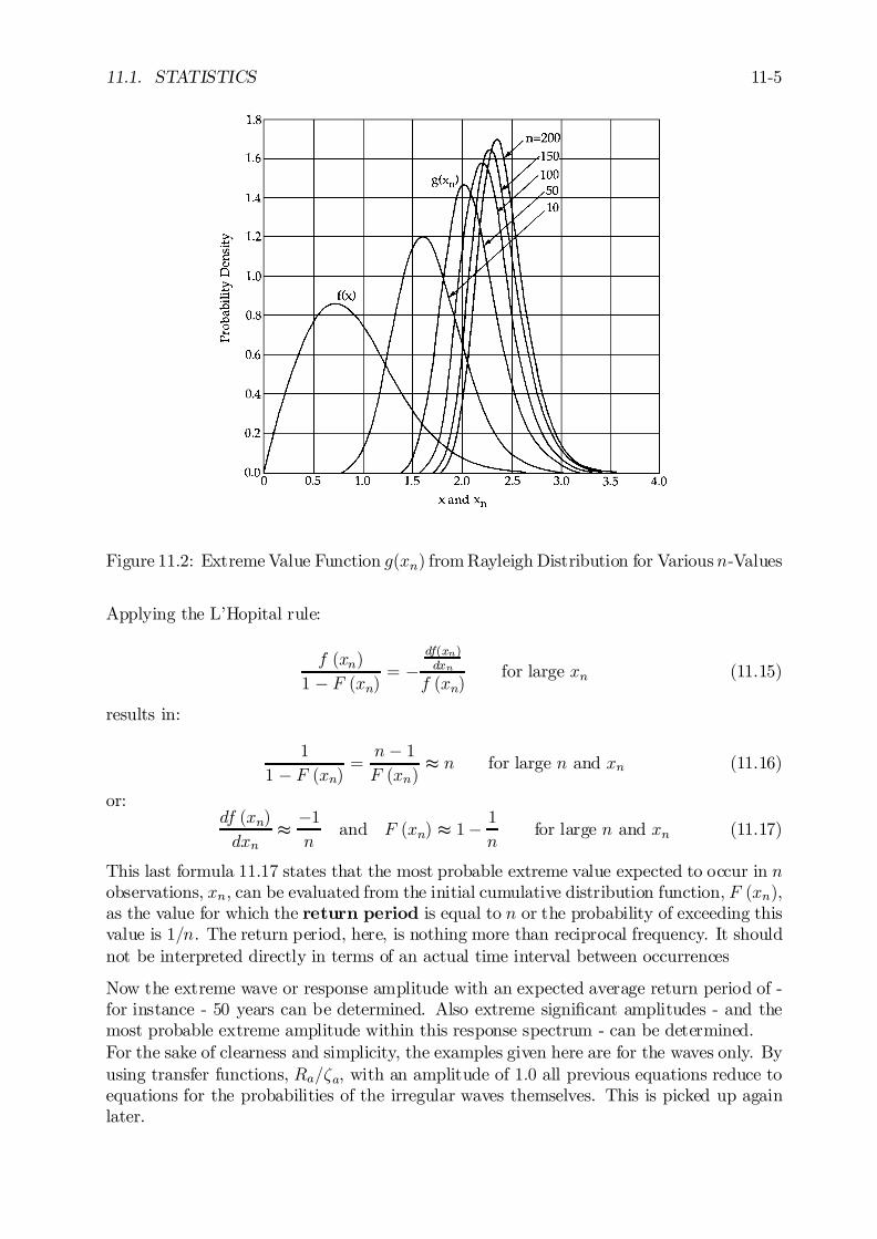
11.1. STATISTICS 11-5
Figure 11.2: Extreme Value Function g(xn) from Rayleigh Distribution for Variousn-Values
Applying the L’Hopital rule:
f (xn)
1 ¡ F (xn)= ¡
df(xn)dxn
f (xn)for large xn (11.15)
results in:
1
1 ¡ F (xn)=n¡ 1F (xn)
t n for large n and xn (11.16)
or:df (xn)
dxnt ¡1n
and F (xn) t 1¡ 1
nfor large n and xn (11.17)
This last formula 11.17 states that the most probable extreme value expected to occur in nobservations, xn, can be evaluated from the initial cumulative distribution function, F (xn),as the value for which the return period is equal to n or the probability of exceeding thisvalue is 1=n. The return period, here, is nothing more than reciprocal frequency. It shouldnot be interpreted directly in terms of an actual time interval between occurrences
Now the extreme wave or response amplitude with an expected average return period of -for instance - 50 years can be determined. Also extreme signi…cant amplitudes - and themost probable extreme amplitude within this response spectrum - can be determined.For the sake of clearness and simplicity, the examples given here are for the waves only. Byusing transfer functions, Ra=³a, with an amplitude of 1:0 all previous equations reduce toequations for the probabilities of the irregular waves themselves. This is picked up againlater.
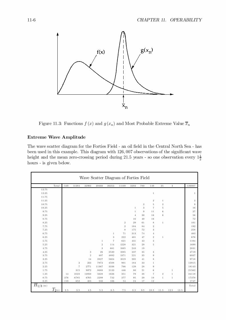
11-6 CHAPTER 11. OPERABILITY
Figure 11.3: Functions f (x) and g (xn) and Most Probable Extreme Value xn
Extreme Wave Amplitude
The wave scatter diagram for the Forties Field - an oil …eld in the Central North Sea - hasbeen used in this example. This diagram with 126; 007 observations of the signi…cant waveheight and the mean zero-crossing period during 21:5 years - so one observation every 11
2
hours - is given below.
Wave Scatter Diagram of Forties Field
Tota l 549 11284 32993 39460 26353 11109 3293 789 149 25 3 126007
12 .75
12 .25 1 1
11 .75
11 .25 2 1 3
10 .75 2 5 2 9
10 .25 1 3 7 5 16
9 .75 1 9 11 6 27
9 .25 4 30 16 6 56
8 .75 16 40 16 72
8 .25 2 29 61 8 1 101
7 .75 2 104 84 2 192
7 .25 8 175 72 3 258
6 .75 1 71 313 74 4 463
6 .25 3 222 401 47 2 1 676
5 .75 1 7 621 431 42 2 1104
5 .25 2 114 1228 321 29 5 1699
4 .75 3 681 1885 243 19 2831
4 .25 3 26 2530 1885 237 35 3 4719
3 .75 2 407 4892 1371 221 35 9 6937
3 .25 14 2827 5604 1019 205 41 8 9718
2 .75 3 233 7972 4588 901 184 33 1 13915
2 .25 7 2771 11367 3336 766 129 28 9 18143
1 .75 315 9872 8688 2133 446 80 21 6 1 21562
1 .25 14 3522 12850 5628 1626 351 79 38 7 2 1 24118
0 .75 376 6785 6765 2299 732 277 95 29 10 1 1 17370
0 .25 159 652 483 240 106 54 24 17 12 1747
H1=3 (m ) Tota l
T2 (s) 2 .5 3 .5 4 .5 5 .5 6 .5 7.5 8 .5 9.5 10 .5 11 .5 12.5 13 .5
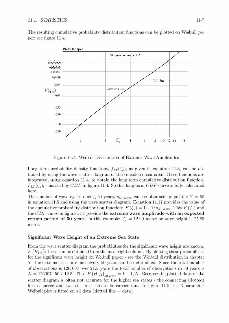
11.1. STATISTICS 11-7
The resulting cumulative probability distribution functions can be plotted on Weibull pa-per; see …gure 11.4.
Figure 11.4: Weibull Distribution of Extreme Wave Amplitudes
Long term probability density functions, fLT (³a), as given in equation 11.3, can be ob-tained by using the wave scatter diagram of the considered sea area. These functions areintegrated, using equation 11.4, to obtain the long term cumulative distribution function,FLT (³a), - marked by CDF in …gure 11.4. So this long term CDF -curve is fully calculatedhere.The number of wave cycles during 50 years, n50 years, can be obtained by putting Y = 50in equation 11.5 and using the wave scatter diagram. Equation 11.17 provides the value ofthe cumulative probability distribution function: F (³a) = 1¡ 1=n50 years. This F (³a) andthe CDF -curve in …gure 11.4 provide the extreme wave amplitude with an expectedreturn period of 50 years; in this example: ³a = 12:90 meter or wave height is 25:80meter.
Signi…cant Wave Height of an Extreme Sea State
From the wave scatter diagram the probabilities for the signi…cant wave height are known,F
¡H1=3
¢; these can be obtained from the most right column. Byplotting these probabilities
for the signi…cant wave height on Weibull paper - see the Weibull distribution in chapter5 - the extreme sea state once every 50 years can be determined. Since the total numberof observations is 126; 007 over 21:5 years the total number of observations in 50 years isN = 126007 ¢ 50 = 12:5. Thus F
¡H1=3
¢50 years = 1 ¡ 1=N . Because the plotted data of the
scatter diagram is often not accurate for the higher sea states - the connecting (dotted)line is curved and twisted - a …t has to be carried out. In …gure 11.5, the 3-parameterWeibull plot is …tted on all data (dotted line = data).

11-8 CHAPTER 11. OPERABILITY
F¡H1=3
¢= 1 ¡ exp
(¡
µH1=3 ¡ a
c
¶b)
(Weibull) (11.18)
Figure 11.5: Probability Distribution of Signi…cant Wave Heights
This plot gives a straight curve for higher sea states and is then used to determine theextreme signi…cant wave height. From the …gure follows that the extreme signi…cantwave height with a return period of 50 years is 11:80 meter.Obviously, the type of …tting is important. How to weigh the importance of the tail? Inthis case, paying more attention to the upper tail would lead to a …t with a higher extremesigni…cant wave height than a simple extrapolation of the data curve.
Extreme Wave Amplitude in an Extreme Sea State
Consider now this extreme sea state with a return period of 50 years - lasting 3 hours,as generally done in o¤shore calculations. Using the formulation for the most probablemaximum, F (³a) = 1¡1=N , the extreme wave amplitude in this sea state can be calculatedfrom the Rayleigh distribution:
P©³a > ³a max (50 years storm)
ª= exp
(¡³2a max (50 years storm)
2 ¢m0³
)=1
N(11.19)
or:
³a max (50 years storm) =q2 ¢m0³ ¢ ln (N) (11.20)
The number of cycles, N , can be determined by using a wave period T2 = 12:0 seconds.This is the average (central) period belonging to the extreme signi…cant wave height of11:80 meter, as obtained from the wave scatter diagram.
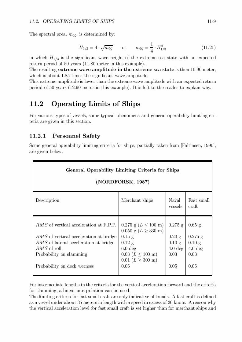
11.2. OPERATING LIMITS OF SHIPS 11-9
The spectral area, m0³, is determined by:
H1=3 = 4 ¢ pm0³ or m0³ =
1
4¢H 2
1=3 (11.21)
in which H1=3 is the signi…cant wave height of the extreme sea state with an expectedreturn period of 50 years (11:80 meter in this example).The resulting extreme wave amplitude in the extreme sea state is then 10:90 meter,which is about 1:85 times the signi…cant wave amplitude.This extreme amplitude is lower than the extreme wave amplitude with an expected returnperiod of 50 years (12:90 meter in this example). It is left to the reader to explain why.
11.2 Operating Limits of Ships
For various types of vessels, some typical phenomena and general operability limiting cri-teria are given in this section.
11.2.1 Personnel Safety
Some general operability limiting criteria for ships, partially taken from [Faltinsen, 1990],are given below.
General Operability Limiting Criteria for Ships
(NORDFORSK, 1987)
Description Merchant ships Naval Fast smallvessels craft
RMS of vertical acceleration at F.P.P. 0.275 g (L · 100 m) 0.275 g 0.65 g0.050 g (L ¸ 330 m)
RMS of vertical acceleration at bridge 0.15 g 0.20 g 0.275 gRMS of lateral acceleration at bridge 0.12 g 0.10 g 0.10 gRMS of roll 6.0 deg 4.0 deg 4.0 degProbability on slamming 0.03 (L · 100 m) 0.03 0.03
0.01 (L ¸ 300 m)Probability on deck wetness 0.05 0.05 0.05
For intermediate lengths in the criteria for the vertical acceleration forward and the criteriafor slamming, a linear interpolation can be used.The limiting criteria for fast small craft are only indicative of trends. A fast craft is de…nedas a vessel under about 35 meters in length with a speed in excess of 30 knots. A reason whythe vertical acceleration level for fast small craft is set higher than for merchant ships and
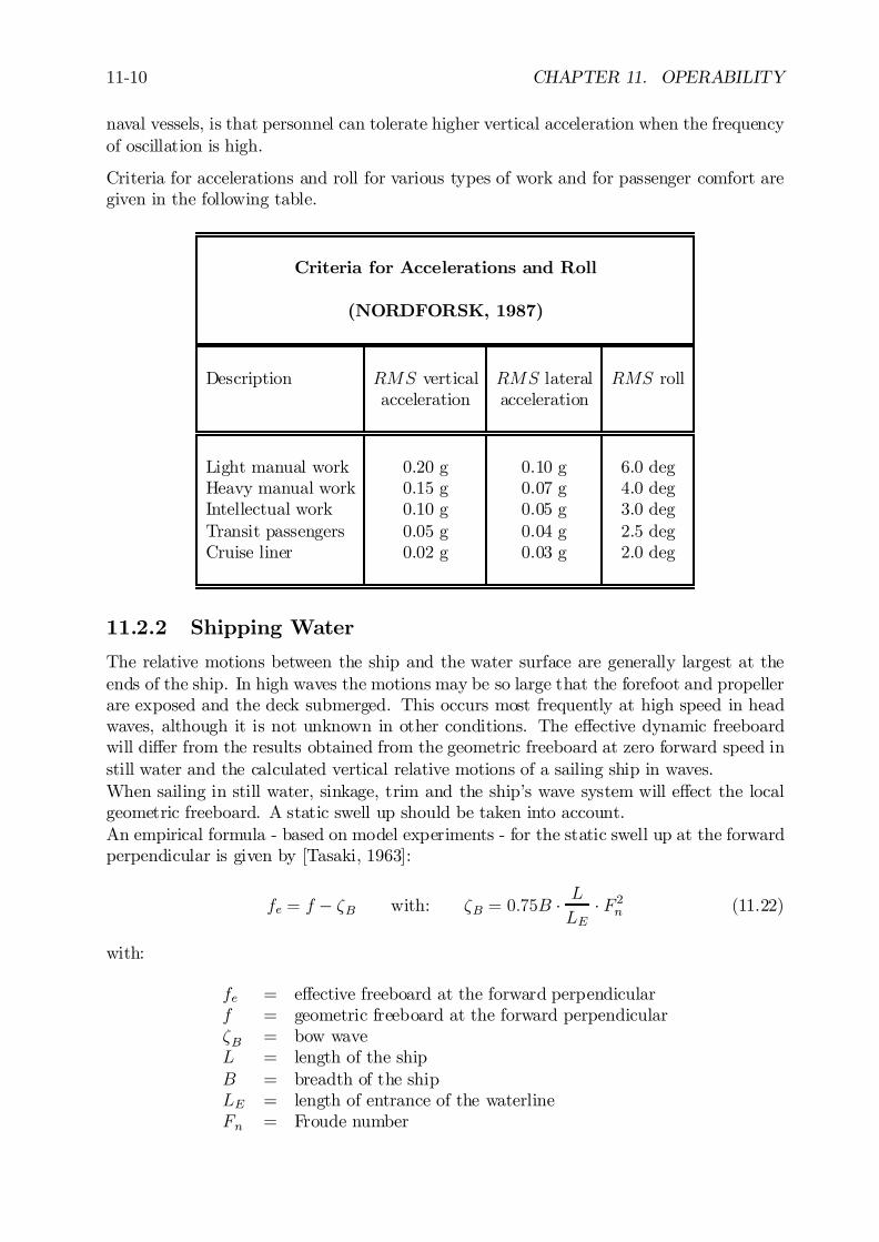
11-10 CHAPTER 11. OPERABILITY
naval vessels, is that personnel can tolerate higher vertical acceleration when the frequencyof oscillation is high.
Criteria for accelerations and roll for various types of work and for passenger comfort aregiven in the following table.
Criteria for Accelerations and Roll
(NORDFORSK, 1987)
Description RMS vertical RMS lateral RMS rollacceleration acceleration
Light manual work 0.20 g 0.10 g 6.0 degHeavy manual work 0.15 g 0.07 g 4.0 degIntellectual work 0.10 g 0.05 g 3.0 degTransit passengers 0.05 g 0.04 g 2.5 degCruise liner 0.02 g 0.03 g 2.0 deg
11.2.2 Shipping Water
The relative motions between the ship and the water surface are generally largest at theends of the ship. In high waves the motions may be so large that the forefoot and propellerare exposed and the deck submerged. This occurs most frequently at high speed in headwaves, although it is not unknown in other conditions. The e¤ective dynamic freeboardwill di¤er from the results obtained from the geometric freeboard at zero forward speed instill water and the calculated vertical relative motions of a sailing ship in waves.When sailing in still water, sinkage, trim and the ship’s wave system will e¤ect the localgeometric freeboard. A static swell up should be taken into account.An empirical formula - based on model experiments - for the static swell up at the forwardperpendicular is given by [Tasaki, 1963]:
fe = f ¡ ³B with: ³B = 0:75B ¢ LLE
¢ F 2n (11.22)
with:
fe = e¤ective freeboard at the forward perpendicularf = geometric freeboard at the forward perpendicular³B = bow waveL = length of the shipB = breadth of the shipLE = length of entrance of the waterlineFn = Froude number
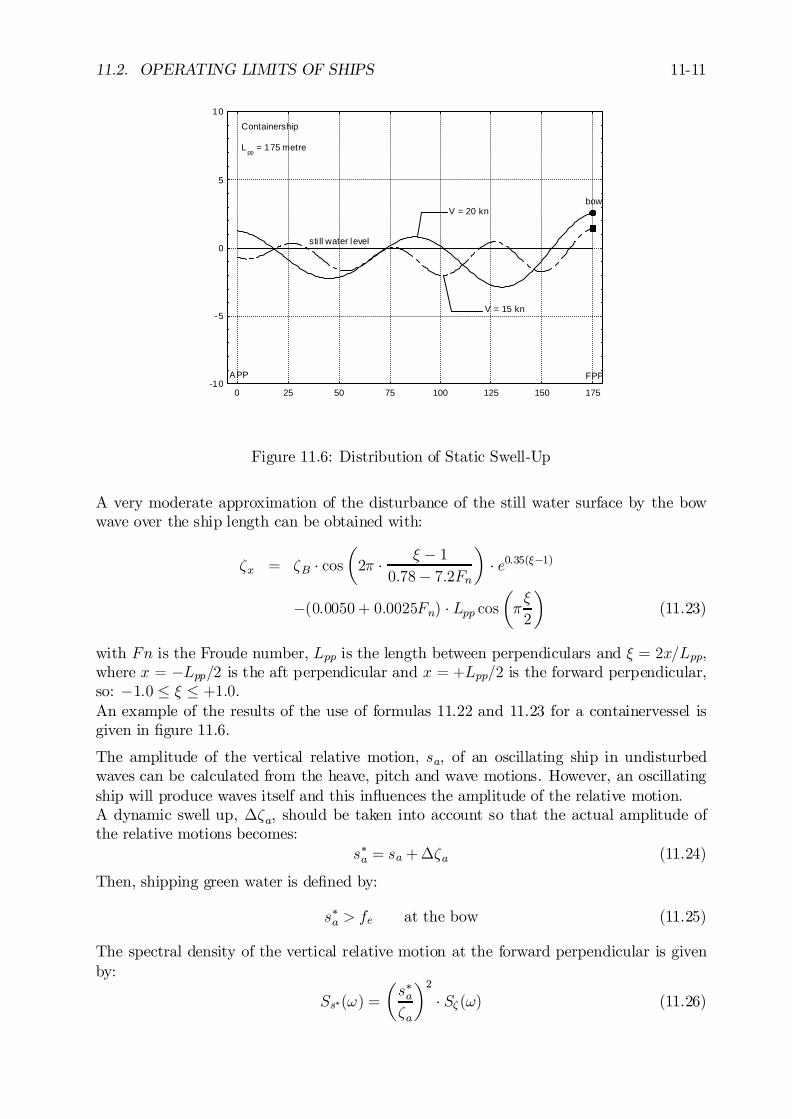
11.2. OPERATING LIMITS OF SHIPS 11-11
-10
-5
0
5
10
0 25 50 75 100 125 150 175
bow
Containership L
pp = 175 metre
sti ll water level
V = 15 kn
V = 20 kn
FPPAPP
Figure 11.6: Distribution of Static Swell-Up
A very moderate approximation of the disturbance of the still water surface by the bowwave over the ship length can be obtained with:
³x = ³B ¢ cosµ2¼ ¢ » ¡ 1
0:78¡ 7:2Fn
¶¢ e0:35(»¡1)
¡(0:0050 + 0:0025Fn) ¢ Lpp cosµ¼»
2
¶(11.23)
with Fn is the Froude number, Lpp is the length between perpendiculars and » = 2x=Lpp,where x = ¡Lpp=2 is the aft perpendicular and x = +Lpp=2 is the forward perpendicular,so: ¡1:0 · » · +1:0.An example of the results of the use of formulas 11.22 and 11.23 for a containervessel isgiven in …gure 11.6.
The amplitude of the vertical relative motion, sa, of an oscillating ship in undisturbedwaves can be calculated from the heave, pitch and wave motions. However, an oscillatingship will produce waves itself and this in‡uences the amplitude of the relative motion.A dynamic swell up, ¢³a, should be taken into account so that the actual amplitude ofthe relative motions becomes:
s¤a = sa +¢³a (11.24)
Then, shipping green water is de…ned by:
s¤a > fe at the bow (11.25)
The spectral density of the vertical relative motion at the forward perpendicular is givenby:
Ss¤(!) =
µs¤a³a
¶2
¢ S³ (!) (11.26)
11-12 CHAPTER 11. OPERABILITY
and the moments are given by:
mns¤ =
1Z
0
Ss¤ (!) ¢ !ne ¢ d! with: n = 0; 1; 2; ::: (11.27)
Using the Rayleigh distribution, the short term probability of shipping green water in agiven storm condition is: ¯
¯P fs¤a > feg = expµ ¡f2e2m0s¤
¶¯¯ (11.28)
The number of times per hour that green water will be shipped in a certain sea state followsfrom the short term probability on shipping green water and the number of oscillations perhour: ¯
¯Nshipping/hour =3600
T2s¤¢ P fs¤a > feg
¯¯ (11.29)
in which T2s¤ = 2¼pm0s¤=m2s¤ is the average zero-crossing period.
11.2.3 Slamming
Slamming is a two-node vibration of the ship caused by suddenly pushing the ship bythe waves. This occurs when the bow of the ship comes completely out of the water andthen ”crashes down” with an impact against the next wave. Slamming in‡uences the localpressures on the hull plating and a local damage can be the result. The impulse natureof the impact also causes internal vibrations which can contribute to structural fatigue inthe ship. Slamming does not necessarily in‡uence the overall vertical displacements of theship signi…cantly. Slamming forces can be very large, but they act on the ship during avery short time.A complete prediction of slamming phenomena is a very complex task, which is beyondthe scope of any existing theory. Slamming impact pressures are a¤ected by the local hullsection shape, the relative velocity between ship and wave at impact, the relative anglebetween the keel and the water surface, the local ‡exibility of the ship’s bottom platingand the overall ‡exibility of the ship’s structure.
Ochi Criterium
[Ochi, 1964] has translated slamming phenomena into requirements for the vertical relativemotions of the ship; he de…ned slamming by:- an emergence of the bow of the ship at 10 per cent of the length aft of the forward
perpendiculars and- at the instant of impact the exceedance of a certain critical vertical relative velocity,
without forward speed e¤ect, between the wave surface and the bow of the ship.
Ochi de…nes the vertical relative displacement and velocity of the water particles withrespect to the keel point of the ship by:
s = ³xb ¡ z + xb ¢ µ_s = _³xb ¡ _z + xb ¢ _µ (11.30)
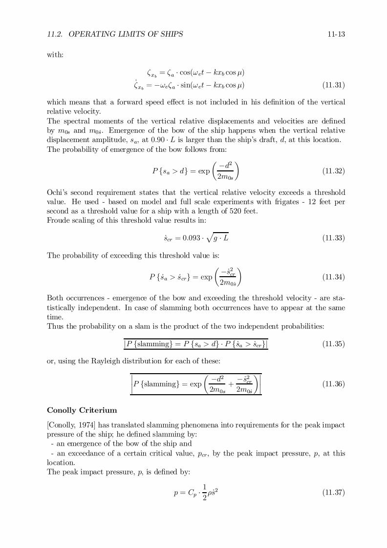
11.2. OPERATING LIMITS OF SHIPS 11-13
with:
³xb = ³a ¢ cos(!et¡ kxb cos¹)_³xb = ¡!e³a ¢ sin(!et¡ kxb cos¹) (11.31)
which means that a forward speed e¤ect is not included in his de…nition of the verticalrelative velocity.The spectral moments of the vertical relative displacements and velocities are de…nedby m0s and m0 _s. Emergence of the bow of the ship happens when the vertical relativedisplacement amplitude, sa, at 0:90 ¢ L is larger than the ship’s draft, d, at this location.The probability of emergence of the bow follows from:
P fsa > dg = expµ ¡d22m0s
¶(11.32)
Ochi’s second requirement states that the vertical relative velocity exceeds a thresholdvalue. He used - based on model and full scale experiments with frigates - 12 feet persecond as a threshold value for a ship with a length of 520 feet.Froude scaling of this threshold value results in:
_scr = 0:093 ¢pg ¢ L (11.33)
The probability of exceeding this threshold value is:
P f _sa > _scrg = expµ ¡ _s2cr2m0_s
¶(11.34)
Both occurrences - emergence of the bow and exceeding the threshold velocity - are sta-tistically independent. In case of slamming both occurrences have to appear at the sametime.Thus the probability on a slam is the product of the two independent probabilities:
jP fslammingg = P fsa > dg ¢ P f _sa > _scrgj (11.35)
or, using the Rayleigh distribution for each of these:
¯¯P fslammingg = exp
µ ¡d22m0s
+¡ _s2cr2m0_s
¶¯¯ (11.36)
Conolly Criterium
[Conolly, 1974] has translated slamming phenomena into requirements for the peak impactpressure of the ship; he de…ned slamming by:- an emergence of the bow of the ship and- an exceedance of a certain critical value, pcr, by the peak impact pressure, p, at this
location.The peak impact pressure, p, is de…ned by:
p = Cp ¢ 12½ _s2 (11.37)
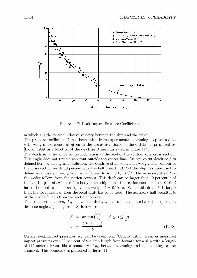
11-14 CHAPTER 11. OPERABILITY
Figure 11.7: Peak Impact Pressure Coe¢cients
in which _s is the vertical relative velocity between the ship and the wave.The pressure coe¢cient Cp has been taken from experimental slamming drop tests datawith wedges and cones, as given in the literature. Some of these data, as presented by[Lloyd, 1989] as a function of the deadrise ¯, are illustrated in …gure 11.7.The deadrise is the angle of the inclination at the keel of the contour of a cross section.This angle does not remain constant outside the center line. An equivalent deadrise ¯ isde…ned here by an engineers solution: the deadrise of an equivalent wedge. The contour ofthe cross section inside 10 percentile of the half breadth B=2 of the ship has been used tode…ne an equivalent wedge with a half breadth: b = 0:10 ¢B=2. The accessory draft t ofthe wedge follows from the section contour. This draft can be larger than 10 percentile ofthe amidships draft d in the fore body of the ship. If so, the section contour below 0:10 ¢ dhas to be used to de…ne an equivalent wedge: t = 0:10 ¢ d. When this draft, t, is largerthan the local draft, d, then the local draft has to be used. The accessory half breadth, b,of the wedge follows from the section contour.Then the sectional area, As, below local draft, t, has to be calculated and the equivalentdeadrise angle ¯ (see …gure 11.8) follows from:
¯ = arctan³ab
´0 · ¯ · 1
2¼
a =2(b ¢ t¡ As)
b(11.38)
Critical peak impact pressures, pcr, can be taken from [Conolly, 1974]. He gives measuredimpact pressures over 30 per cent of the ship length from forward for a ship with a lengthof 112 meters. From this, a boundary of pcr between slamming and no slamming can beassumed. This boundary is presented in …gure 11.9.
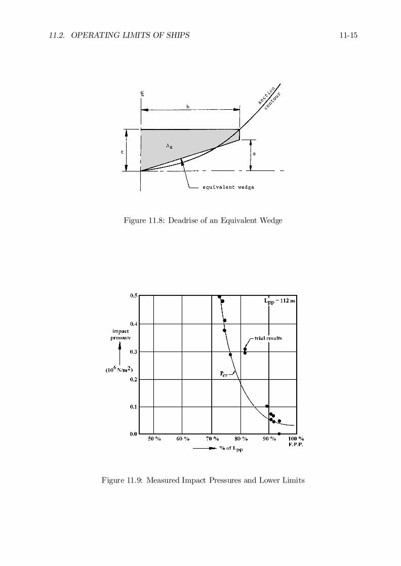
11.2. OPERATING LIMITS OF SHIPS 11-15
Figure 11.8: Deadrise of an Equivalent Wedge
Figure 11.9: Measured Impact Pressures and Lower Limits
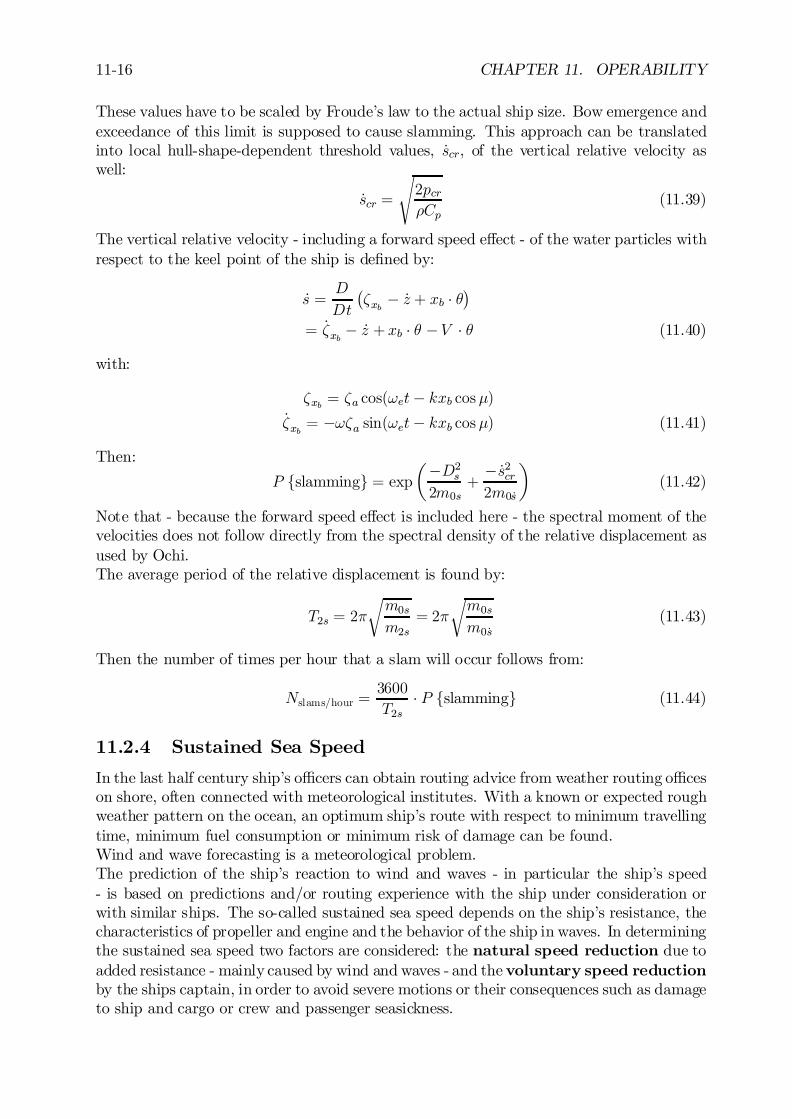
11-16 CHAPTER 11. OPERABILITY
These values have to be scaled by Froude’s law to the actual ship size. Bow emergence andexceedance of this limit is supposed to cause slamming. This approach can be translatedinto local hull-shape-dependent threshold values, _scr, of the vertical relative velocity aswell:
_scr =
s2pcr½Cp
(11.39)
The vertical relative velocity - including a forward speed e¤ect - of the water particles withrespect to the keel point of the ship is de…ned by:
_s =D
Dt
¡³xb ¡ _z + xb ¢ µ
¢
= _³xb ¡ _z + xb ¢ µ ¡V ¢ µ (11.40)
with:
³xb = ³a cos(!et¡ kxb cos¹)_³xb = ¡!³a sin(!et¡ kxb cos¹) (11.41)
Then:
P fslammingg = expµ¡D2s2m0s
+¡ _s2cr2m0_s
¶(11.42)
Note that - because the forward speed e¤ect is included here - the spectral moment of thevelocities does not follow directly from the spectral density of the relative displacement asused by Ochi.The average period of the relative displacement is found by:
T2s = 2¼
rm0sm2s
= 2¼
rm0s
m0_s
(11.43)
Then the number of times per hour that a slam will occur follows from:
Nslams/hour =3600
T2s¢ P fslammingg (11.44)
11.2.4 Sustained Sea Speed
In the last half century ship’s o¢cers can obtain routing advice from weather routing o¢ceson shore, often connected with meteorological institutes. With a known or expected roughweather pattern on the ocean, an optimum ship’s route with respect to minimum travellingtime, minimum fuel consumption or minimum risk of damage can be found.Wind and wave forecasting is a meteorological problem.The prediction of the ship’s reaction to wind and waves - in particular the ship’s speed- is based on predictions and/or routing experience with the ship under consideration orwith similar ships. The so-called sustained sea speed depends on the ship’s resistance, thecharacteristics of propeller and engine and the behavior of the ship in waves. In determiningthe sustained sea speed two factors are considered: the natural speed reduction due toadded resistance - mainly caused by wind and waves - and the voluntary speed reductionby the ships captain, in order to avoid severe motions or their consequences such as damageto ship and cargo or crew and passenger seasickness.
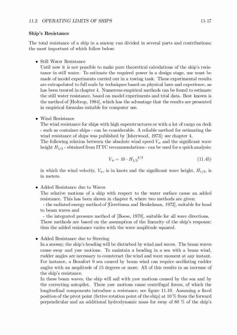
11.2. OPERATING LIMITS OF SHIPS 11-17
Ship’s Resistance
The total resistance of a ship in a seaway can divided in several parts and contributions;the most important of which follow below:
² Still Water ResistanceUntil now it is not possible to make pure theoretical calculations of the ship’s resis-tance in still water. To estimate the required power in a design stage, use must bemade of model experiments carried out in a towing tank. These experimental resultsare extrapolated to full scale by techniques based on physical laws and experience, ashas been treated in chapter 4. Numerous empirical methods can be found to estimatethe still water resistance, based on model experiments and trial data. Best known isthe method of [Holtrop, 1984], which has the advantage that the results are presentedin empirical formulas suitable for computer use.
² Wind ResistanceThe wind resistance for ships with high superstructures or with a lot of cargo on deck- such as container ships - can be considerable. A reliable method for estimating thewind resistance of ships was published by [Isherwood, 1973]; see chapter 4.The following relation between the absolute wind speed Vw and the signi…cant waveheightH1=3 - obtained from ITTC recommendations - can be used for a quick analysis:
Vw = 10 ¢H1=32=3 (11.45)
in which the wind velocity, Vw, is in knots and the signi…cant wave height, H1=3, isin meters.
² Added Resistance due to WavesThe relative motions of a ship with respect to the water surface cause an addedresistance. This has been shown in chapter 8, where two methods are given:- the radiated energy method of [Gerritsma and Beukelman, 1972], suitable for head
to beam waves and- the integrated pressure method of [Boese, 1970], suitable for all wave directions.
These methods are based on the assumption of the linearity of the ship’s response;thus the added resistance varies with the wave amplitude squared.
² Added Resistance due to SteeringIn a seaway, the ship’s heading will be disturbed by wind and waves. The beam wavescause sway and yaw motions. To maintain a heading in a sea with a beam wind,rudder angles are necessary to counteract the wind and wave moment at any instant.For instance, a Beaufort 9 sea caused by beam wind can require oscillating rudderangles with an amplitude of 15 degrees or more. All of this results in an increase ofthe ship’s resistance.In these beam waves, the ship will sail with yaw motions caused by the sea and bythe correcting autopilot. These yaw motions cause centrifugal forces, of which thelongitudinal components introduce a resistance; see …gure 11.10. Assuming a …xedposition of the pivot point (…ctive rotation point of the ship) at 10% from the forwardperpendicular and an additional hydrodynamic mass for sway of 80 % of the ship’s
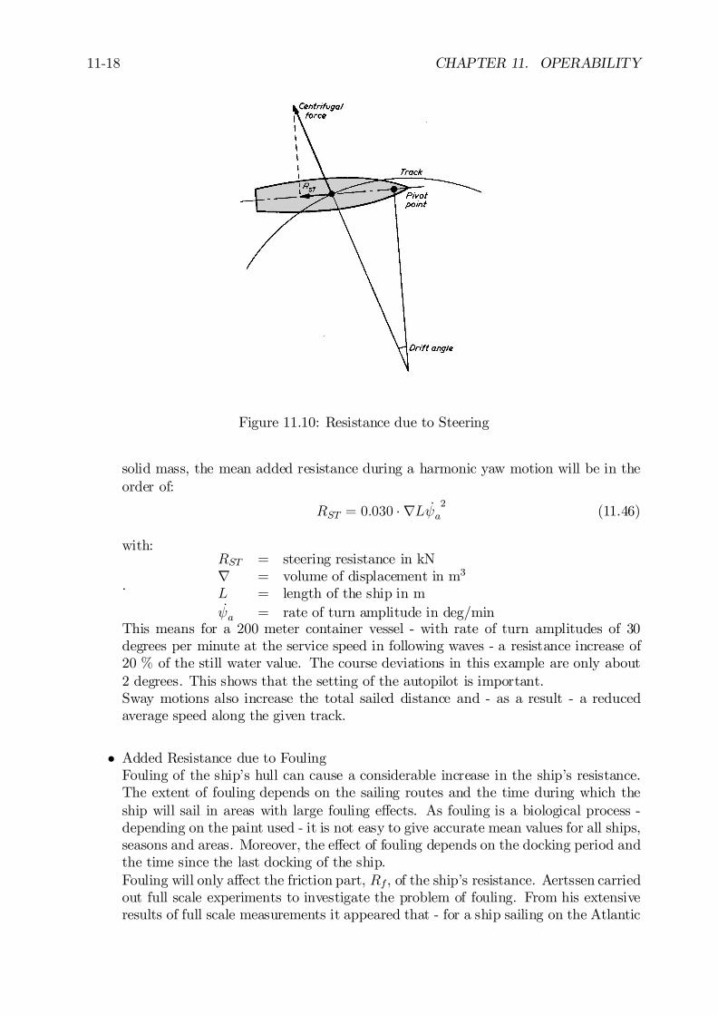
11-18 CHAPTER 11. OPERABILITY
Figure 11.10: Resistance due to Steering
solid mass, the mean added resistance during a harmonic yaw motion will be in theorder of:
RST = 0:030 ¢ rL _Ãa2
(11.46)
with:
.
RST = steering resistance in kNr = volume of displacement in m3
L = length of the ship in m_Ãa = rate of turn amplitude in deg/min
This means for a 200 meter container vessel - with rate of turn amplitudes of 30degrees per minute at the service speed in following waves - a resistance increase of20 % of the still water value. The course deviations in this example are only about2 degrees. This shows that the setting of the autopilot is important.Sway motions also increase the total sailed distance and - as a result - a reducedaverage speed along the given track.
² Added Resistance due to FoulingFouling of the ship’s hull can cause a considerable increase in the ship’s resistance.The extent of fouling depends on the sailing routes and the time during which theship will sail in areas with large fouling e¤ects. As fouling is a biological process -depending on the paint used - it is not easy to give accurate mean values for all ships,seasons and areas. Moreover, the e¤ect of fouling depends on the docking period andthe time since the last docking of the ship.Fouling will only a¤ect the friction part, Rf , of the ship’s resistance. Aertssen carriedout full scale experiments to investigate the problem of fouling. From his extensiveresults of full scale measurements it appeared that - for a ship sailing on the Atlantic
11.2. OPERATING LIMITS OF SHIPS 11-19
route - the e¤ect of fouling on the frictional resistance will be in the order of:
¢RfRf
¢ 100% = 3:6 ¢ ya +40 ¢ yd1 + 2 ¢ yd
(11.47)
in which ya is the age of the ship in years and yd is the year since the last docking.This means for instance, an increase of the frictional resistance by about 30 % for aship with an age of …ve years and a last docking one year previously.However, the overall e¤ect on the total resistance is smaller and depends on speedand ship type. With low speeds and full ship forms - e.g. tankers - the frictional re-sistance is the major part of the total resistance, whereas the wave-making resistancedominates in the case of high speed container ships. This means that the e¤ect offouling is much larger for tankers than for container ships.An investigation by [Journée, 1976b] of log data of a 200,000 tdw tanker, sailing fromEurope to the Persian Gulf, showed an increase of the still water resistance for fullload and ballast condition as 26 to 29 % one year after the last docking and 47 to52 % two years after the last docking. After the oil crisis in the early seventies theseships reduced power by 50 %, resulting in a speed reduction for the clean hull from16 to 13 knots. To maintain this speed two years after the last docking the powerof a fully loaded ship had to be increased from 50 to over 80 %. This behavior isvisualized in …gure 11.11 as an example to show that fouling is a factor which shouldnot be neglected in sustained sea speed calculations.
Figure 11.11: Increase of Required Propulsion Power due to Fouling
The sum of these contributions provides the total resistance of the ship under operationalconditions.
11-20 CHAPTER 11. OPERABILITY
Propulsion
The propeller behind a ship can be considered as an energy transformer: torque with enginespeed will be transformed into thrust with a speed of advance of the propeller, relative tothe mean velocity of the incoming water. At a constant engine setting there should bean equilibrium between the engine speed and the ship’s speed in such a way that twoconditions are ful…lled: the torque required by the propeller must be in equilibrium withthe torque delivered by the engine and the thrust delivered by the propeller must be inequilibrium with the total resistance of the ship in the self-propelled condition. This hasbeen treated in chapter 4.
² PropellerThe characteristics of an open water propeller in its normal operating range are usu-ally expressed in its thrust coe¢cient, KT, and torque coe¢cient, KQ, as a functionof the speed (or advance) ratio, J :
KT =T
½D4n2KQ =
Q
½D5n2J =
VenD
(11.48)
with T is thrust, Q is torque, ½ is density of water, D is propeller diameter, n isnumber of propeller revolutions per second and Ve is relative speed of advance.These characteristics depend on the number of propeller blades, the pitch ratio andthe expanded blade area ratio and can be obtained by means of open water modelexperiments. Results of such experiments with systematically varied propeller seriescan be found in various publications.One of the best known is the Wageningen B-propeller series of MARIN. Over 120systematically varied propeller models have been tested and the results are given inpolynomials, together with a correction for scale e¤ect. These results are valid forthe open water condition.For the ”behind the ship condition” the open water torque must be multiplied by therelative rotative e¢ciency ´R:
´R =Qopen water
Qbehind ship(11.49)
which varies from about ´R = 1:04 for single screw ships to about ´R = 0:97 for twinscrew ships. This e¢ciency re‡ects the di¤erence in torque in the wake and in openwater at the same thrust.The relative speed of the water, Ve, into the propeller disc is not equal to the forwardship speed, V . A wake fraction, w, should be taken into account:
Ve = V ¢ (1 ¡ w) (11.50)
This wake fraction varies from 0.2 to 0.4 and can be obtained directly from modelexperiments - taking into account the scale e¤ect - or from empirical formulas givenin the literature.From model experiments it appears that the wake fraction is hardly a¤ected by anincrease of the propeller loading due to a resistance increase, caused by - for instance- towing a barge, motions in waves, etc.As discussed in chapter 4, the thrust of the propeller, T , is not equal to the ship’s
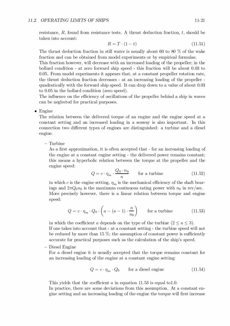
11.2. OPERATING LIMITS OF SHIPS 11-21
resistance, R, found from resistance tests. A thrust deduction fraction, t, should betaken into account:
R = T ¢ (1¡ t) (11.51)
The thrust deduction fraction in still water is usually about 60 to 80 % of the wakefraction and can be obtained from model experiments or by empirical formulae.This fraction however, will decrease with an increased loading of the propeller; in thebollard condition - at zero forward ship speed - this fraction will be about 0.03 to0.05. From model experiments it appears that, at a constant propeller rotation rate,the thrust deduction fraction decreases - at an increasing loading of the propeller -quadratically with the forward ship speed. It can drop down to a value of about 0.03to 0.05 in the bollard condition (zero speed).The in‡uence on the e¢ciency of oscillations of the propeller behind a ship in wavescan be neglected for practical purposes.
² EngineThe relation between the delivered torque of an engine and the engine speed at aconstant setting and an increased loading in a seaway is also important. In thisconnection two di¤erent types of engines are distinguished: a turbine and a dieselengine.
– TurbineAs a …rst approximation, it is often accepted that - for an increasing loading ofthe engine at a constant engine setting - the delivered power remains constant;this means a hyperbolic relation between the torque at the propeller and theengine speed:
Q= c ¢ ´m ¢ Q0 ¢ n0n
for a turbine (11.52)
in which c is the engine setting, ´m is the mechanical e¢ciency of the shaft bear-ings and 2¼Q0n0 is the maximum continuous rating power with n0 in rev/sec.More precisely however, there is a linear relation between torque and enginespeed:
Q = c ¢ ´m ¢Q0 ¢µa ¡ (a ¡ 1) ¢ n
n0
¶for a turbine (11.53)
in which the coe¢cient a depends on the type of the turbine (2 · a · 3).If one takes into account that - at a constant setting - the turbine speed will notbe reduced by more than 15 %; the assumption of constant power is su¢cientlyaccurate for practical purposes such as the calculation of the ship’s speed.
– Diesel EngineFor a diesel engine it is usually accepted that the torque remains constant foran increasing loading of the engine at a constant engine setting:
Q = c ¢ ´m ¢Q0 for a diesel engine (11.54)
This yields that the coe¢cient a in equation 11.53 is equal to1.0.In practice, there are some deviations from this assumption. At a constant en-gine setting and an increasing loading of the engine the torque will …rst increase
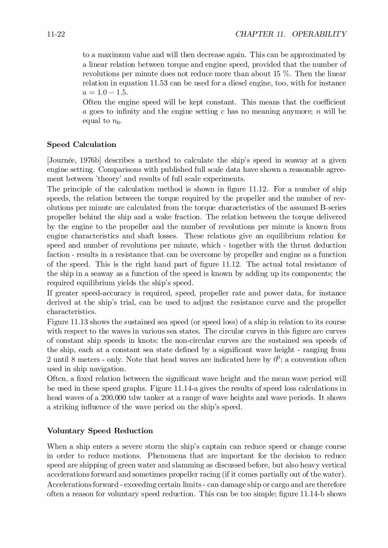
11-22 CHAPTER 11. OPERABILITY
to a maximum value and will then decrease again. This can be approximated bya linear relation between torque and engine speed, provided that the number ofrevolutions per minute does not reduce more than about 15 %. Then the linearrelation in equation 11.53 can be used for a diesel engine, too, with for instancea = 1:0¡ 1:5.Often the engine speed will be kept constant. This means that the coe¢cienta goes to in…nity and the engine setting c has no meaning anymore; n will beequal to n0.
Speed Calculation
[Journée, 1976b] describes a method to calculate the ship’s speed in seaway at a givenengine setting. Comparisons with published full scale data have shown a reasonable agree-ment between ’theory’ and results of full scale experiments.The principle of the calculation method is shown in …gure 11.12. For a number of shipspeeds, the relation between the torque required by the propeller and the number of rev-olutions per minute are calculated from the torque characteristics of the assumed B-seriespropeller behind the ship and a wake fraction. The relation between the torque deliveredby the engine to the propeller and the number of revolutions per minute is known fromengine characteristics and shaft losses. These relations give an equilibrium relation forspeed and number of revolutions per minute, which - together with the thrust deductionfaction - results in a resistance that can be overcome by propeller and engine as a functionof the speed. This is the right hand part of …gure 11.12. The actual total resistance ofthe ship in a seaway as a function of the speed is known by adding up its components; therequired equilibrium yields the ship’s speed.If greater speed-accuracy is required, speed, propeller rate and power data, for instancederived at the ship’s trial, can be used to adjust the resistance curve and the propellercharacteristics.Figure 11.13 shows the sustained sea speed (or speed loss) of a ship in relation to its coursewith respect to the waves in various sea states. The circular curves in this …gure are curvesof constant ship speeds in knots; the non-circular curves are the sustained sea speeds ofthe ship, each at a constant sea state de…ned by a signi…cant wave height - ranging from2 until 8 meters - only. Note that head waves are indicated here by 00; a convention oftenused in ship navigation.Often, a …xed relation between the signi…cant wave height and the mean wave period willbe used in these speed graphs. Figure 11.14-a gives the results of speed loss calculations inhead waves of a 200,000 tdw tanker at a range of wave heights and wave periods. It showsa striking in‡uence of the wave period on the ship’s speed.
Voluntary Speed Reduction
When a ship enters a severe storm the ship’s captain can reduce speed or change coursein order to reduce motions. Phenomena that are important for the decision to reducespeed are shipping of green water and slamming as discussed before, but also heavy verticalaccelerations forward and sometimes propeller racing (if it comes partially out of the water).Accelerations forward - exceeding certain limits - can damage ship or cargo and are thereforeoften a reason for voluntary speed reduction. This can be too simple; …gure 11.14-b shows
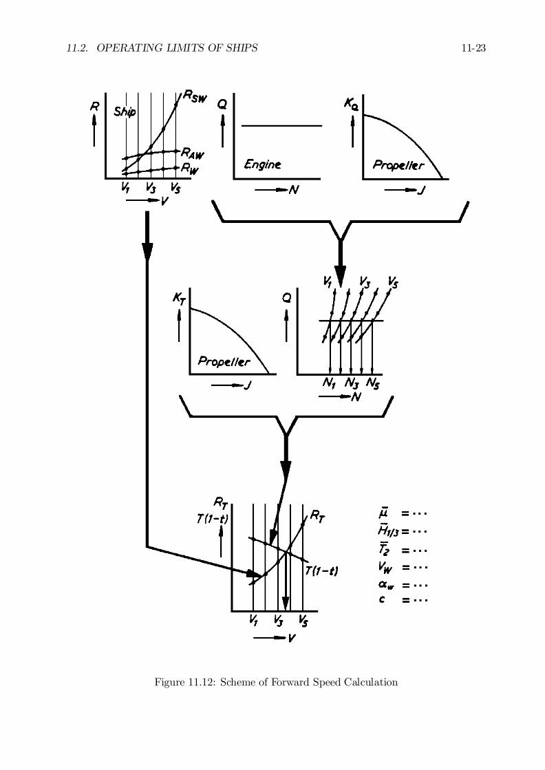
11.2. OPERATING LIMITS OF SHIPS 11-23
Figure 11.12: Scheme of Forward Speed Calculation
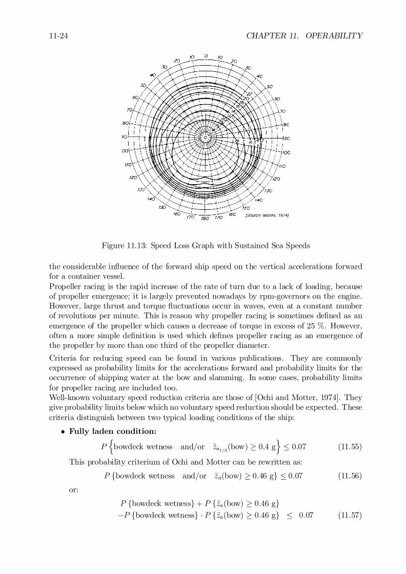
11-24 CHAPTER 11. OPERABILITY
Figure 11.13: Speed Loss Graph with Sustained Sea Speeds
the considerable in‡uence of the forward ship speed on the vertical accelerations forwardfor a container vessel.Propeller racing is the rapid increase of the rate of turn due to a lack of loading, becauseof propeller emergence; it is largely prevented nowadays by rpm-governors on the engine.However, large thrust and torque ‡uctuations occur in waves, even at a constant numberof revolutions per minute. This is reason why propeller racing is sometimes de…ned as anemergence of the propeller which causes a decrease of torque in excess of 25 %. However,often a more simple de…nition is used which de…nes propeller racing as an emergence ofthe propeller by more than one third of the propeller diameter.
Criteria for reducing speed can be found in various publications. They are commonlyexpressed as probability limits for the accelerations forward and probability limits for theoccurrence of shipping water at the bow and slamming. In some cases, probability limitsfor propeller racing are included too.Well-known voluntary speed reduction criteria are those of [Ochi and Motter, 1974]. Theygive probability limits below which no voluntary speed reduction should be expected. Thesecriteria distinguish between two typical loading conditions of the ship:
² Fully laden condition:
Pnbowdeck wetness and/or Äza1=3(bow) ¸ 0:4 g
o· 0:07 (11.55)
This probability criterium of Ochi and Motter can be rewritten as:
P fbowdeck wetness and/or Äza(bow) ¸ 0:46 gg · 0:07 (11.56)
or:
P fbowdeck wetnessg+ P fÄza(bow) ¸ 0:46 gg¡P fbowdeck wetnessg ¢ P fÄza(bow) ¸ 0:46 gg · 0:07 (11.57)
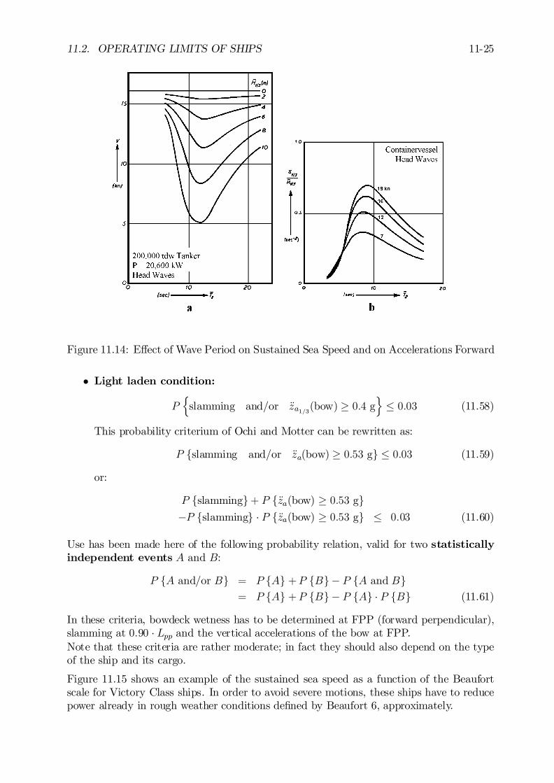
11.2. OPERATING LIMITS OF SHIPS 11-25
Figure 11.14: E¤ect of Wave Period on Sustained Sea Speed and on Accelerations Forward
² Light laden condition:
Pnslamming and/or Äza1=3(bow) ¸ 0:4 g
o· 0:03 (11.58)
This probability criterium of Ochi and Motter can be rewritten as:
P fslamming and/or Äza(bow) ¸ 0:53 gg · 0:03 (11.59)
or:
P fslammingg+ P fÄza(bow) ¸ 0:53 gg¡P fslammingg ¢ P fÄza(bow) ¸ 0:53 gg · 0:03 (11.60)
Use has been made here of the following probability relation, valid for two statisticallyindependent events A and B:
P fA and/or Bg = P fAg +P fBg ¡ P fA and Bg= P fAg +P fBg ¡ P fAg ¢ P fBg (11.61)
In these criteria, bowdeck wetness has to be determined at FPP (forward perpendicular),slamming at 0:90 ¢ Lpp and the vertical accelerations of the bow at FPP.Note that these criteria are rather moderate; in fact they should also depend on the typeof the ship and its cargo.
Figure 11.15 shows an example of the sustained sea speed as a function of the Beaufortscale for Victory Class ships. In order to avoid severe motions, these ships have to reducepower already in rough weather conditions de…ned by Beaufort 6, approximately.
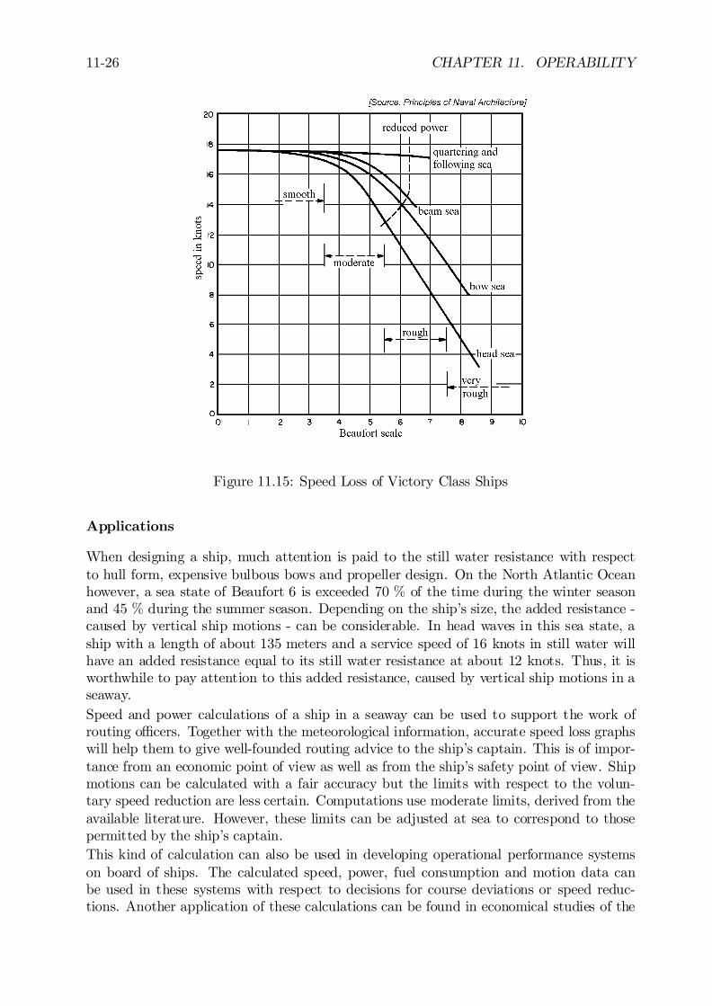
11-26 CHAPTER 11. OPERABILITY
Figure 11.15: Speed Loss of Victory Class Ships
Applications
When designing a ship, much attention is paid to the still water resistance with respectto hull form, expensive bulbous bows and propeller design. On the North Atlantic Oceanhowever, a sea state of Beaufort 6 is exceeded 70 % of the time during the winter seasonand 45 % during the summer season. Depending on the ship’s size, the added resistance -caused by vertical ship motions - can be considerable. In head waves in this sea state, aship with a length of about 135 meters and a service speed of 16 knots in still water willhave an added resistance equal to its still water resistance at about 12 knots. Thus, it isworthwhile to pay attention to this added resistance, caused by vertical ship motions in aseaway.Speed and power calculations of a ship in a seaway can be used to support the work ofrouting o¢cers. Together with the meteorological information, accurate speed loss graphswill help them to give well-founded routing advice to the ship’s captain. This is of impor-tance from an economic point of view as well as from the ship’s safety point of view. Shipmotions can be calculated with a fair accuracy but the limits with respect to the volun-tary speed reduction are less certain. Computations use moderate limits, derived from theavailable literature. However, these limits can be adjusted at sea to correspond to thosepermitted by the ship’s captain.This kind of calculation can also be used in developing operational performance systemson board of ships. The calculated speed, power, fuel consumption and motion data canbe used in these systems with respect to decisions for course deviations or speed reduc-tions. Another application of these calculations can be found in economical studies of the
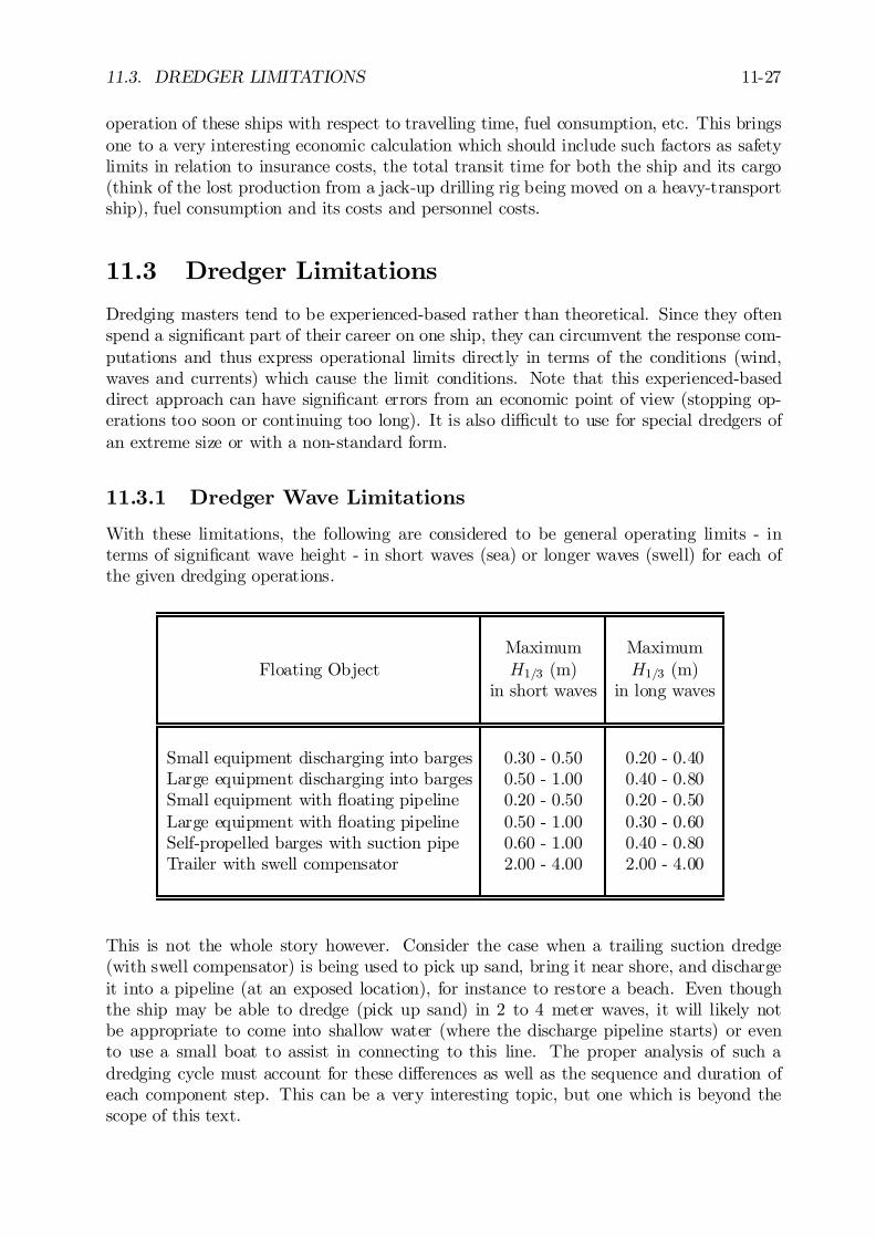
11.3. DREDGER LIMITATIONS 11-27
operation of these ships with respect to travelling time, fuel consumption, etc. This bringsone to a very interesting economic calculation which should include such factors as safetylimits in relation to insurance costs, the total transit time for both the ship and its cargo(think of the lost production from a jack-up drilling rig being moved on a heavy-transportship), fuel consumption and its costs and personnel costs.
11.3 Dredger Limitations
Dredging masters tend to be experienced-based rather than theoretical. Since they oftenspend a signi…cant part of their career on one ship, they can circumvent the response com-putations and thus express operational limits directly in terms of the conditions (wind,waves and currents) which cause the limit conditions. Note that this experienced-baseddirect approach can have signi…cant errors from an economic point of view (stopping op-erations too soon or continuing too long). It is also di¢cult to use for special dredgers ofan extreme size or with a non-standard form.
11.3.1 Dredger Wave Limitations
With these limitations, the following are considered to be general operating limits - interms of signi…cant wave height - in short waves (sea) or longer waves (swell) for each ofthe given dredging operations.
Maximum MaximumFloating Object H1=3 (m) H1=3 (m)
in short waves in long waves
Small equipment discharging into barges 0.30 - 0.50 0.20 - 0.40Large equipment discharging into barges 0.50 - 1.00 0.40 - 0.80Small equipment with ‡oating pipeline 0.20 - 0.50 0.20 - 0.50Large equipment with ‡oating pipeline 0.50 - 1.00 0.30 - 0.60Self-propelled barges with suction pipe 0.60 - 1.00 0.40 - 0.80Trailer with swell compensator 2.00 - 4.00 2.00 - 4.00
This is not the whole story however. Consider the case when a trailing suction dredge(with swell compensator) is being used to pick up sand, bring it near shore, and dischargeit into a pipeline (at an exposed location), for instance to restore a beach. Even thoughthe ship may be able to dredge (pick up sand) in 2 to 4 meter waves, it will likely notbe appropriate to come into shallow water (where the discharge pipeline starts) or evento use a small boat to assist in connecting to this line. The proper analysis of such adredging cycle must account for these di¤erences as well as the sequence and duration ofeach component step. This can be a very interesting topic, but one which is beyond thescope of this text.
11-28 CHAPTER 11. OPERABILITY
11.3.2 Dredger Current Limitations
If the anchors hold su¢ciently, it makes a considerable di¤erence as to whether the ship canwork with the current or whether it has to work at an angle to the current, as for instance acutter suction dredger. For a cutter suction dredger the situation is particularly dangerouswhen the current is directed against the ladder side. The current direction in this …gureapproaches from the ladder side, which is convenient in that it helps supply material tothe suction mouth in the cutter. On the other hand, when the current is too strong orthe deviation angle gets too large the anchoring system on the ladder can fail. When thishappens, the dredge will swing around her spud pile which can result in a broken dischargepipe, a broken (or bent) spud pile, a broken ladder when it hits the channel side or even acapsized dredger, if the spud pile and/or the ladder do not fail.Here, again, dredging masters are experience-based. For most of the larger cutter suctiondredgers the safe limit can be estimated at about 2 knots velocity of the current. For bucketdredgers and stationary dredgers the limit is about 3 knots provided the anchorage andfreeboard of the ship are su¢cient. Self-propelled barges are preferable when working instrong currents; this avoids the need for moorings between the dredge and transportationbarge.
Chapter 12
WAVE FORCES ON SLENDERCYLINDERS
12.1 Introduction
Chapters 6 through 11 have handled the hydromechanics of large (‡oating) bodies in thesea. Attention now switches to the hydromechanics of slender cylinders. Examples of suchcylinders include the leg or brace of an o¤shore space truss structure, a pipeline or evenan umbilical cable extending down to some form of remotely controlled vehicle.
12.2 Basic Assumptions and De…nitions
A slender cylinder in this discussion implies that its diameter is small relative to the wavelength.The cylinder diameter,D, should be much less than the wave length, ¸; the methodsto be discussed here are often usable as long as D
¸< about 0:1 to 0:2.
Derivations are done for a unit length of cylinder. Force relationships will yield a force perunit length. This relationship must then be integrated over the cylinder length to yield atotal force. The implications of this unit length approach combined with the restrictionto slender cylinders is that the ambient water motions in the immediate vicinity of thecylinder are all about the same at any instant in time. This is (assumed to be) true bothvertically and horizontally; the spatial variation in the undisturbed ‡ow near a unit lengthof cylinder is simply neglected. A similar assumption was made for the heaving cylinder inchapter 6, but this is not usually the case with a ship or other large structure as discussedin the previous chapters.The absence of a spatial variation in the ambient ‡ow as one moves from place to place nearthe cylinder, makes it possible to characterize the ‡ow in the entire region of the cylinderby the ambient ‡ow at one characteristic location. The axis of the cylinder is chosen asthat location; this simpli…es the bookkeeping.The ‡ow around this cylinder segment will be considered to be two-dimensional - quiteanalogous to strip theory for ships except that the axis of the in…nitely long cylinder is notgenerally horizontal as it was for a ship. Flow components and any resulting forces parallel
0J.M.J. Journée and W.W. Massie, ”OFFSHORE HYDROMECHANICS”, First Edition, January 2001,Delft University of Technology. For updates see web site: http://www.shipmotions.nl.
12-2 CHAPTER 12. WAVE FORCES ON SLENDER CYLINDERS
to the cylinder axis are neglected; all forces are caused by the ‡ow - and later cylindermotion - components perpendicular to the cylinder axis.The axis system used here is identical to that used for the waves in chapter 5, see …gure5.2. The origin lies at the still water level with the positive z-axis directed upward. Thewave moves along the x-axis in the positive direction.The resulting water motions come directly from chapter 5 as well:
u =@©w@x
=dx
dt= ³a! ¢ coshk (h + z)
sinhkh¢ cos (kx¡ !t) (12.1)
w =@©w@z
=dz
dt= ³a! ¢ sinh k (h + z)
sinh kh¢ sin (kx ¡ !t) (12.2)
These can be simpli…ed for the following discussions, however. Since the location, x; of thecylinder element is more or less …xed, the kx term in the above equations can be dropped.For the moment, it is simplest to consider a vertical cylinder so that equation 12.1 willyield the desired ‡ow velocity. All of this yields an undisturbed horizontal ‡ow velocitygiven by:
u(z; t) = ³a! ¢ coshk (h+ z)sinhkh
¢ cos (¡!t) (12.3)
or at any chosen elevation, z:
u(t) = ua cos(¡!t) (12.4)
and since cos(¡!t) = cos(!t) the sign is often dropped so that:
u(t) = ua cos(!t) (12.5)
in which:
ua = amplitude the wave-generated horizontalwater velocity at elevation z (m/s)
! = wave frequency (rad/s)
Note that the elevation dependence in equation 12.3 has been included in ua in 12.4; thisdependence is not included speci…cally in the most of the following discussion.Since the ‡ow is time dependent, it will have a horizontal acceleration as well. This canbe worked out to be:
_u(t) = ¡! ua sin (!t) (12.6)
The acceleration amplitude is thus given by:
_ua = ! ua (12.7)
Since potential theory describes waves so well, the above relations are assumed to hold forany undisturbed wave ‡ow - even when viscosity is involved.
12.3 Force Components in Oscillating Flows
It is convenient to derive the relationships in this section for a smooth-surfaced verticalcylinder. This restriction will be relaxed later in this chapter, however. Since potential‡ows are so convenient for computations, this discussion of forces in oscillating ‡ows startswith this idealization. The unit length of cylinder being considered is thus vertical andsubmerged at some convenient depth below the water surface.
12.3. FORCE COMPONENTS IN OSCILLATING FLOWS 12-3
12.3.1 Inertia Forces
Remember from chapter 3 that D’Alembert proved that there is no resultant drag forcewhen a time-independent potential ‡ow is present. Here, it is the e¤ect of the ‡owaccelerations that is of concern.Consider …rst the undisturbed ambient (surrounding) ‡ow without any cylinder in it. Ac-cording to Newton’s second law of motion, accelerations result from forces; this is univer-sally true. Thus, the horizontal acceleration of the ambient ‡ow must be driven by a forcein the water which, in turn, must come from a horizontal pressure gradient. This pressuregradient is present, even when there is no cylinder in the ‡ow. By examining the pressuregradient force on a di¤erential ’block’ of ‡uid, one discovers that:
dp
dx= ½
du
dt= ½ ¢ _u (12.8)
which is nothing more than Newton’s second law applied to a ‡uid.
Given this information, what happens when a cylinder is inserted into this pressure and ‡ow…eld? This question is answered using an approach which has the advantage of physicallyexplaining the separate contributions of two separate inertia force components; a faster,but less ’transparent’ derivation will be given later.
Pressure Gradient Force
One must ’drill a hole’ in the ambient pressure gradient …eld in order to ’insert’ the cylinder.For now, the fact that the cylinder wall is impervious is neglected completely; the ‡ow isstill undisturbed. Any force which this undisturbed pressure …eld exerts on the cylindercan be computed by integrating this pressure around the perimeter of the circular hole.This integral yields, knowing that the cylinder is symmetrical with respect to the x-axisand has a unit length:
Fx1(t) = 2 ¢Z ¼
0
p(R; µ; t) R cosµ ¢ 1 ¢ dµ (12.9)
in which p(R; µ; t) is the undisturbed pressure (N/m2) on the perimeter of the circle andR is the cylinder radius (m).The resulting force is computed just as was done in chapter 3, using …gure 3.16.Since the pressure di¤erence across the cylinder at any distance, y; away from the x-axisis:
¢p = ½ ¢ _u ¢¢x (12.10)
where ¢x is the width of the cylinder at distance y from its axis. The integral can besimpli…ed again so that:
Fx1(t) = 2 ¢Z ¼
2
0
¢p(R; µ; t) ¢R ¢ cos µ ¢ dµ (12.11)
After integrating one gets:Fx1(t) = ½ ¼ R
2 ¢ _u(t) (12.12)
12-4 CHAPTER 12. WAVE FORCES ON SLENDER CYLINDERS
In which one should recognize ¼R2½ as the mass, M1; of ‡uid displaced by the unit lengthof cylinder - the mass of ‡uid one would have ’removed’ when ’drilling the hole’ in thepressure gradient …eld.This inertia force term stems from the pressure gradient already present in the accelerating‡ow - even before the cylinder was installed. It is equal to the product of the mass of waterdisplaced by the cylinder and the acceleration already present in the undisturbed ‡ow.This force component is fully equivalent to the Froude Krilov force mentioned in chapter6.
Disturbance Force
The cylinder was not allowed to disturb the ‡ow when Fx1 was computed; this error is nowcorrected. Obviously, the cylinder is impermeable; ‡uid cannot actually ‡ow through thecylinder wall. The cylinder geometry forces the ‡uid to go around it modifying all the localvelocities and thus accelerations. This can only occur if a force is exerted on the ‡uid, andthis force can only come from the cylinder.Figure 3.12, which can be found in chapter 3, shows how the streamlines diverge andconverge around a cylinder in a potential ‡ow. One way to evaluate the extra force causingthis total disturbance …eld is to examine the kinetic energy change caused by the cylinderas was done by [Lamb, 1932]. He evaluated the kinetic energy represented by the entire(disturbed) ‡ow …eld around the cylinder and subtracted from that value the kinetic energyof the undisturbed ‡ow in the same - theoretically in…nite - region. This yields in equationform:
E =
1ZZ
cyl: wall
1
2½ ¢ [u (x; y; t)]2 dx ¢ dy ¡
1ZZ
cyl: wall
1
2½ ¢ u21(t) ¢ dx ¢ dy (12.13)
It is convenient to associate this energy with some sort of equivalent mass, M2; movingwith the ambient (undisturbed ‡ow) velocity, u1; so that:
E =1
2M2 u
21 (12.14)
Lamb discovered that:M2 = ¼ R
2 ½ (12.15)
or that M2 is simply the mass of ‡uid displaced by the cylinder segment (just as was M1)so that:
Fx2 = ¼ R2 ½ ¢ _u(t) (12.16)
Note that Fx2 has the same form as Fx1 and that they both have the same phase as well.Fx2 is analogous to the part of the di¤raction force which was in phase with the shipacceleration in chapter 6.A thoughtful reader may wonder why this second force component, Fx2 , was not presentin a constant current; after all, that cylinder was then impervious to the ‡ow, too. Theanswer to this question lies in the fact that Fx2 does not result from the pattern itself, butrather from its continuous build-up and break-down which occurs only in a time-dependent‡ow. In a constant current there is no time dependent change and thus no Fx2.
12.3. FORCE COMPONENTS IN OSCILLATING FLOWS 12-5
Resultant Inertia Force
Potential theory indicates that the resultant force on a …xed cylinder in an oscillating ‡owis the sum of two terms:
Fx1(t) = ½ ¼ R2 ¢ _u1(t) from the ’hole’ in the undisturbed pressure gradient in theambient ‡ow. This is also know as the Froude-Krilov force.
Fx2(t) = ½ ¼ R2 ¢ _u1(t) from the ‡ow disturbance caused by the impervious cylinder.
The resultant force is then:
FI(t) = Fx1(t) + Fx2(t)
= 2 ¢ ¼ R2 ½ ¢ _u(t) (12.17)
Note that because this is still a potential ‡ow, there is no drag force. Also, since there isno circulation, there is no lift, either.
Alternate Direct Calculation Approach
Another, possibly faster way to calculate the ‡ow disturbance force coe¢cient starts withthe potential function for an oscillating cylinder in still water. This approach is completelyanalogous to that used in chapter 6 to determine the added mass of a ‡oating body. Onestarts directly with the potential function just as was done there, and uses the Bernoulliequation to calculate the pressure on the cylinder surface and then integrate this as wasdone in chapter 3 to determine the resultant force.
Experimental Inertia Coe¢cients
The theoretical value of 2 in equation 12.17, above, is usually replaced by an experimentalcoe¢cient, CM - often called the inertia coe¢cient. Remember that the theoreticalvalue of 2 is made up of 1 from Fx1 (the ambient pressure …eld) and 1 from Fx2, the‡ow disturbance caused by the cylinder. In practice the 1 from the ambient pressure…eld is usually considered to be acceptable; potential theory predicts the water motion inundisturbed waves well. The coe¢cient from Fx2 is much less certain; the vortices in thewake (in a real, [not potential!] ‡ow) disturb the theoretical ‡ow pattern used to determineFx2. This is taken into account by using a value Ca - a ’coe¢cient of added mass’ -instead. Usually Ca < 1. Note that Ca is quite analogous to the hydrodynamic mass usedin chapter 6. This is all summarize in the table below.
ForceComponent
ForceTerm
ExperimentalCoe¢cient
TheoreticalValue
ExperimentalValue
Froude-Krylov Fx1 1 1 1Disturbance Fx2 Ca 1 Usually < 1
Inertia FI CM 2 Usually 1 to 2
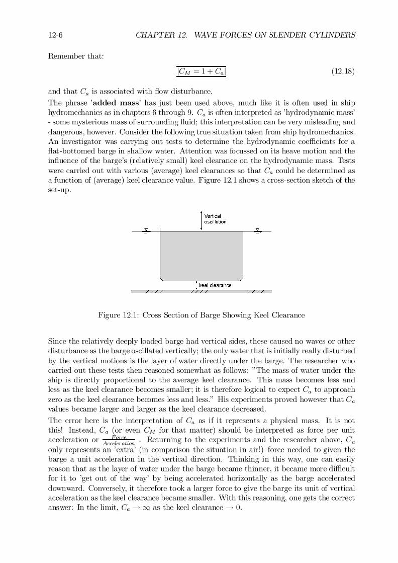
12-6 CHAPTER 12. WAVE FORCES ON SLENDER CYLINDERS
Remember that:
jCM = 1+ Caj (12.18)
and that Ca is associated with ‡ow disturbance.
The phrase ’added mass’ has just been used above, much like it is often used in shiphydromechanics as in chapters 6 through 9. Ca is often interpreted as ’hydrodynamic mass’- some mysterious mass of surrounding ‡uid; this interpretation can be very misleading anddangerous, however. Consider the following true situation taken from ship hydromechanics.An investigator was carrying out tests to determine the hydrodynamic coe¢cients for a‡at-bottomed barge in shallow water. Attention was focussed on its heave motion and thein‡uence of the barge’s (relatively small) keel clearance on the hydrodynamic mass. Testswere carried out with various (average) keel clearances so that Ca could be determined asa function of (average) keel clearance value. Figure 12.1 shows a cross-section sketch of theset-up.
Figure 12.1: Cross Section of Barge Showing Keel Clearance
Since the relatively deeply loaded barge had vertical sides, these caused no waves or otherdisturbance as the barge oscillated vertically; the only water that is initially really disturbedby the vertical motions is the layer of water directly under the barge. The researcher whocarried out these tests then reasoned somewhat as follows: ”The mass of water under theship is directly proportional to the average keel clearance. This mass becomes less andless as the keel clearance becomes smaller; it is therefore logical to expect Ca to approachzero as the keel clearance becomes less and less.” His experiments proved however that Cavalues became larger and larger as the keel clearance decreased.
The error here is the interpretation of Ca as if it represents a physical mass. It is notthis! Instead, Ca (or even CM for that matter) should be interpreted as force per unitacceleration or Force
Acceleration. Returning to the experiments and the researcher above, Ca
only represents an ’extra’ (in comparison the situation in air!) force needed to given thebarge a unit acceleration in the vertical direction. Thinking in this way, one can easilyreason that as the layer of water under the barge became thinner, it became more di¢cultfor it to ’get out of the way’ by being accelerated horizontally as the barge accelerateddownward. Conversely, it therefore took a larger force to give the barge its unit of verticalacceleration as the keel clearance became smaller. With this reasoning, one gets the correctanswer: In the limit, Ca ! 1 as the keel clearance ! 0:
12.3. FORCE COMPONENTS IN OSCILLATING FLOWS 12-7
Fixed Cylinder in Waves
For a …xed cylinder in waves, one is confronted with both Fx1 and Fx2 so that equation12.17 becomes:
FI(t) = Fx1(t) +Fx2(t)
= ½¼
4CM D2 ¢ _u(t) (12.19)
in which:
FI(t) = inertia force per unit cylinder length (N/m)½ = mass density of the ‡uid (kg/m3)CM = dimensionless inertia coe¢cient (-)_u(t) = time dependent undisturbed ‡ow acceleration (m/s2)
CM has a theoretical value of 2 in a potential ‡ow.
Oscillating Cylinder in Still Water
One might reason that the ‡ow around an oscillating cylinder in still water would bekinematically identical to that of an oscillating ‡ow past a …xed cylinder and that theresulting forces would be identical. This is not the case, however.There is no ambient dynamic pressure gradient present in still water so that the …rst inertiaforce term above, Fx1 the Froude-Krilov force, is now identically equal to zero. Thus, ifthe cylinder is oscillating such that its velocity is given by:
_X(t) = a cos(!t) (12.20)
then the resultant hydrodynamic inertia force on the cylinder will be:
FI(t) = ¡Fx2(t) = ¡Ca ¢ ¼ R2 ½ ¢ ÄX (t) (12.21)
The minus sign indicates that the hydrodynamic resisting force is opposite to the directionof cylinder acceleration. The value of Ca will generally not be larger than its theoreticalvalue of 1. Note as well that if one is measuring forces within an instrumented pile ona segment of this oscillating (accelerating) cylinder, one will usually also measure a forcecomponent proportional to the mass times acceleration of the (solid) cylinder element itself.Force measurements in the lab are often corrected for this by …rst measuring forces whileoscillating the cylinder in air before the basin is …lled with water. This force is usuallyconsidered to be the inertia force of the measuring element itself. Only a slight error ismade here by neglecting the aerodynamic resistance caused by the accelerating ‡ow patternin the still air.
12.3.2 Drag Forces
Experiments have shown (see chapter 4) that a drag force proportional to U2 and thecylinder diameter, D; is caused by a constant current; it is only reasonable to expect asimilar force to be present in a time-dependent real ‡ow as well. Since the drag force is inthe same direction - has the same sign - as the velocity in an oscillating ‡ow, the constant
12-8 CHAPTER 12. WAVE FORCES ON SLENDER CYLINDERS
current, U2; is commonly replaced by its time-dependent counterpart, u(t) ju(t)j in orderto maintain a proper sign. Substituting relationships for u(t) and working this out yields:
FD(t) =1
2½ CD D u2a ¢ cos(!t) jcos(!t)j (12.22)
in which:
FD(t) = drag force per unit length of cylinder (N/m)CD = dimensionless drag coe¢cient (-)D = cylinder diameter (m)ua = water velocity amplitude (m/s)! = circular water oscillation frequency (rad/s)t = time (s)
One should not, however, expect the values of CD for an oscillating ‡ow to correspondwith those found in chapter 4 for a constant ‡ow. Instead, they will have to be determinedagain in a time-dependent ‡ow.
12.4 Morison Equation
J.E. Morison, a graduate student at the University of California at the time, wanted topredict wave forces on an exposed vertical pile; see [Morison et al., 1950]. He simply su-perimposed the linear inertia force (from potential theory and oscillating ‡ows) and theadapted quadratic drag force (from real ‡ows and constant currents) to get the followingresultant force (per unit length):
F (t) = Finertia(t) + Fdrag(t) (12.23)
or:
¯¯F (t) = ¼
4½ CMD2 ¢ _u(t) + 1
2½ CDD ¢ u(t) ju(t)j
¯¯ (12.24)
in which the …rst of these two terms is the inertia force and the second represents the dragforce.Note that in equations 12.24 the drag and inertia force components are 90± out of phasewith each other when seen as functions of time. This is a direct consequence of the phaseshift between velocity and acceleration in an oscillatory motion; check equations 12.4 and12.6 if necessary. Examples of this will be shown during the discussion of coe¢cients andtheir determination below; see …gure 12.2 later in this chapter as well.
12.4.1 Experimental Discovery Path
Morison formulated his equation simply by hypothesizing that the superposition of twoseparate and well know phenomena (drag in a current and hydrodynamic inertia in anaccelerating ‡ow) would yield a viable solution for a vertical pile in waves. This sectionexplains how one comes to the same equation via experiments much like those for ships.Readers should know from earlier chapters that a common technique in marine hydrody-namics is to oscillate a body with a chosen displacement amplitude in still water and to
12.4. MORISON EQUATION 12-9
record its displacement and the force, F (t) acting on it as functions of time. Further, theforce record is resolved into two components: one in phase with the acceleration and onein phase with the velocity.The …rst is determined by multiplying F (t) by ¡ cos(!t) and integrating the result to getan inertia force; the second comes from the integral of the product of F (t) and sin(!t) toyield a component in phase with velocity.
One single test might not tell too much, but if testing were done with di¤erent excitationamplitudes, but at constant frequency (or period), then a plot of the amplitude of theinertia force component versus the oscillation acceleleration amplitude would be linear; theplot of the drag force amplitude as a function of velocity amplitude would be quadratic.Similarly, comparison of test results carried out with cylinders of di¤erent diameter wouldshow that the inertia force component was proportional to D2, while the drag force wouldbe linearly proportional to D.
Putting all this together would indicate that the force on a cylinder was of the form:
F (t) = A ¢D2 ¢ _u(t) + B ¢D ¢ [u(t) ¢ ju(t)j] (12.25)
in which A and B are constants. It is then simple enough to use dimensional analysis andcommon sense to express the unknown coe¢cients, A and B as:
A =¼
4½ ¢ Ca and B =
1
2½ ¢ CD (12.26)
12.4.2 Morison Equation Coe¢cient Determination
In this section, a vertical cylinder is assumed to be …xed in a horizontal sinusoidal oscillatory‡ow. The force per unit length acting on the cylinder can be predicted using the Morisonequation with two empirical coe¢cients:
¯¯F (t) = +¼
4½ CM D2 ¢ _u(t) + 1
2½ CD D ¢ u(t) ju(t)j
¯¯ (12.27)
The values of the dimensionless force coe¢cients CD and CM can be determined experi-mentally in a variety of ways. The …rst step, however, is always to get a recording of theforce, F; as a function of time, t. A characteristic of the ‡ow - usually the velocity - willform the second time function.
Experimental Setup
These measurements can be made in a variety of test set-ups.
1. Oscillating ‡ows can be generated in a large U-tube. Unfortunately the ‡ow canonly oscillate with a limited frequency range - the natural oscillation frequency forthe installation - unless an expensive driving system is installed. An advantageof a U-tube, on the other hand, is that its oscillating ‡ow is relatively ’pure’ andturbulence-free. A discussion continues about the applicability of results from suchidealized tests in …eld situations, however. This topic will come up again later in thischapter.
12-10 CHAPTER 12. WAVE FORCES ON SLENDER CYLINDERS
2. A second method is to impose forced oscillations to a cylinder in still water. The‡ow - when seen from the perspective of the cylinder - appears similar to that in aU-tube but the inertia force is not the same. Review the material above about Ca tounderstand why this is so.
3. A third possibility is to place a vertical cylinder in regular waves. The waves aregenerated by a wave maker located at one end of the experimental tank; they areabsorbed on an arti…cial beach at the other end. In this case it is often the waveheight (actually the water surface elevation) which is measured as a function of time.The horizontal water velocity and acceleration at the location of the cylinder are inthis latter case determined using linear wave theory - see chapter 5:
u(z; t) =! H
2¢ cosh [k (z + h)]
sinh (k ¢ h) ¢ cos (!t)
= ua(z) ¢ cos (!t) (12.28)
_u(z; t) = ¡ !2 H
2¢ cosh [k (z + h)]
sinh (k ¢ h) ¢ sin (!t)
= ¡! ¢ ua(z) ¢ sin (!t) (12.29)
in which:
! = 2¼=T = wave frequency (rad/s)k = 2¼=¸ = wave number (rad/m)z = elevation (+ is upward) from the still water level (m)H = wave height (m)h = water depth (m)T = wave period (s)¸ = wave length (m)ua(z) = amplitude of horizontal water velocity component (m/s)
Note that even though ua is now a function of z; this will not really complicate matterswhen studying the forces on a short segment of a cylinder. The change in ua over such ashort distance can be neglected.
With any of these methods, the resultant force on a section of the cylinder is often measuredby mounting that section on a set of leaf springs which are equipped with strain gauges.These - via a Wheatstone bridge circuit and a proper calibration - provide the force record,F (t) to use in conjunction with the measured or computed u(t) and _u(t).
Data Processing
Once the necessary data time series have been obtained, one is still faced with the problemof determining the appropriate CD and CM values. Here, again, one has several optionsdependent upon the computer facilities available.
Several methods are presented here, primarily for reference purposes:
1. Morison’s MethodMorison, himself, suggested a simple method to determine the two unknown coe¢-cients, see [Morison et al., 1950]. His method was elegant in that it was possible to
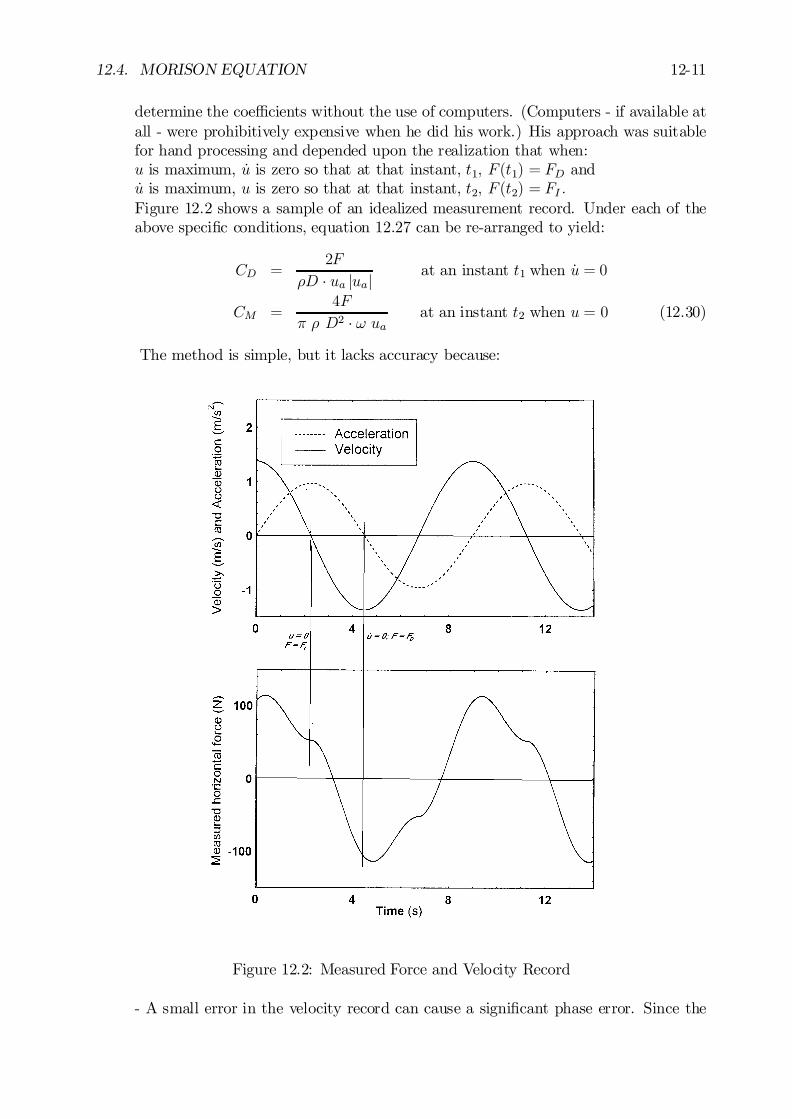
12.4. MORISON EQUATION 12-11
determine the coe¢cients without the use of computers. (Computers - if available atall - were prohibitively expensive when he did his work.) His approach was suitablefor hand processing and depended upon the realization that when:u is maximum, _u is zero so that at that instant, t1; F (t1) = FD and_u is maximum, u is zero so that at that instant, t2; F (t2) = FI :Figure 12.2 shows a sample of an idealized measurement record. Under each of theabove speci…c conditions, equation 12.27 can be re-arranged to yield:
CD =2F
½D ¢ ua juajat an instant t1 when _u = 0
CM =4F
¼ ½ D2 ¢ ! uaat an instant t2 when u = 0 (12.30)
The method is simple, but it lacks accuracy because:
Figure 12.2: Measured Force and Velocity Record
- A small error in the velocity record can cause a signi…cant phase error. Since the
12-12 CHAPTER 12. WAVE FORCES ON SLENDER CYLINDERS
curve of F (t) can be steep (especially when determining CD in …gure 12.2), this cancause quite some error in this coe¢cient. The e¤ect on CM is usually smaller.- Information from only two instants in the time record is used to determine thecoe¢cients; the rest is thrown away.Morison reduced errors by averaging the coe¢cients over a large number of measure-ments (wave periods).One might try to use this same approach at other time instants in the record. Theonly di¢culty, however, is that one is then confronted with a single equation (for Fat that instant) but with two unknown coe¢cients. This cannot be solved uniquely.A second equation could be created by examining the situation at a second, indepen-dent time instant. A generalization of this would be to use the data pairs at everyinstant with a least squares …tting technique. This is discussed below, but only afteranother approach using Fourier series has been presented.
2. Fourier Series ApproachAn entirely di¤erent method for determining the drag and inertia coe¢cients is basedupon the comparison of similar terms in each of two Fourier series: One for the watermotion and one for the force. Appendix C summarizes the theory behind Fourierseries.Since modern laboratory data records are stored at discrete time steps (instead ofas continuous signals), the integrals needed to evaluate the Fourier coe¢cients arereplaced by equivalent sums.Looking at this in a bit more detail, the water velocity and acceleration is already ina nice form as given in equation 12.28. A single Fourier series term is su¢cient toschematize this quite exactly. Since the inertia force, FI , is also well behaved, it canbe ’captured’ with a single Fourier series term as well.
The only remaining problem is the series development of the drag term; this requiresthe development of a function of form:
f (t) = A cos(!t) ¢ j cos (!t)j (12.31)
This has been worked out in Appendix C as well. The resulting coe¢cients (giventhere as well) for the …rst harmonic development of the quadratic drag turn out tobe:FourierCoe¢cient ValueConstant, a0 0Cosine, a1 8
3¼¢ A = 0:849 ¢ A
Sine, b1 0
As shown in Appendix C, the drag force, dependent upon u juj, develops into a seriesof odd-numbered harmonics in a Fourier series; only the …rst harmonic terms are usedhere. Since this has an amplitude of 8
3¼times the original signal, one must multiply
the …rst order harmonic of the force in phase with the velocity by a factor 3 ¼8 to get
the amplitude of the quadratic drag force.Once this has been done, then the determination of CD and CM from the analysis ofthe compete force signal, F (t) is completely straightforward. Since the inertia forcecomponent shows up now in the b1 term of the series development, the results are:
CD =3 ¼
4 ½ D¢ a1 and CM =
4
¼ D2 ½¢ b1! ua
(12.32)
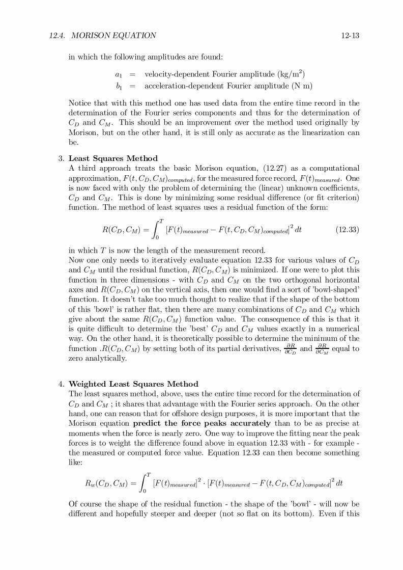
12.4. MORISON EQUATION 12-13
in which the following amplitudes are found:
a1 = velocity-dependent Fourier amplitude (kg/m2)
b1 = acceleration-dependent Fourier amplitude (N m)
Notice that with this method one has used data from the entire time record in thedetermination of the Fourier series components and thus for the determination ofCD and CM . This should be an improvement over the method used originally byMorison, but on the other hand, it is still only as accurate as the linearization canbe.
3. Least Squares MethodA third approach treats the basic Morison equation, (12.27) as a computationalapproximation, F (t; CD; CM)computed, for the measured force record, F (t)measured. Oneis now faced with only the problem of determining the (linear) unknown coe¢cients,CD and CM . This is done by minimizing some residual di¤erence (or …t criterion)function. The method of least squares uses a residual function of the form:
R(CD ; CM) =
Z T
0
[F (t)measured ¡ F (t; CD; CM)computed]2 dt (12.33)
in which T is now the length of the measurement record.Now one only needs to iteratively evaluate equation 12.33 for various values of CDand CM until the residual function, R(CD; CM) is minimized. If one were to plot thisfunction in three dimensions - with CD and CM on the two orthogonal horizontalaxes and R(CD; CM) on the vertical axis, then one would …nd a sort of ’bowl-shaped’function. It doesn’t take too much thought to realize that if the shape of the bottomof this ’bowl’ is rather ‡at, then there are many combinations of CD and CM whichgive about the same R(CD ; CM) function value. The consequence of this is that itis quite di¢cult to determine the ’best’ CD and CM values exactly in a numericalway. On the other hand, it is theoretically possible to determine the minimum of thefunction .R(CD; CM) by setting both of its partial derivatives, @R
@CDand @R
@CMequal to
zero analytically.
4. Weighted Least Squares MethodThe least squares method, above, uses the entire time record for the determination ofCD and CM ; it shares that advantage with the Fourier series approach. On the otherhand, one can reason that for o¤shore design purposes, it is more important that theMorison equation predict the force peaks accurately than to be as precise atmoments when the force is nearly zero. One way to improve the …tting near the peakforces is to weight the di¤erence found above in equation 12.33 with - for example -the measured or computed force value. Equation 12.33 can then become somethinglike:
Rw(CD ; CM) =
Z T
0
[F (t)measured]2 ¢ [F (t)measured ¡F (t; CD; CM)computed]2 dt
Of course the shape of the residual function - the shape of the ’bowl’ - will now bedi¤erent and hopefully steeper and deeper (not so ‡at on its bottom). Even if this
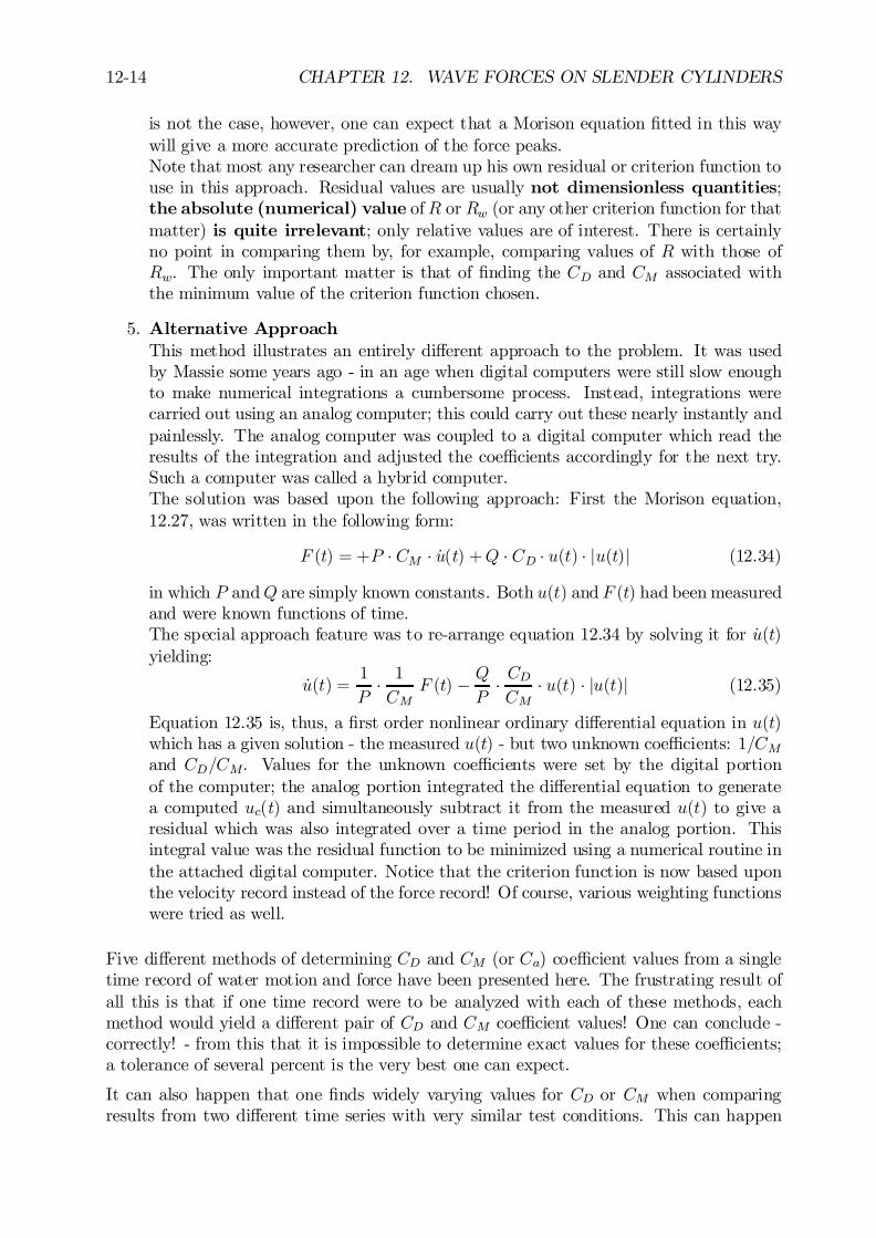
12-14 CHAPTER 12. WAVE FORCES ON SLENDER CYLINDERS
is not the case, however, one can expect that a Morison equation …tted in this waywill give a more accurate prediction of the force peaks.Note that most any researcher can dream up his own residual or criterion function touse in this approach. Residual values are usually not dimensionless quantities;the absolute (numerical) value ofR or Rw (or any other criterion function for thatmatter) is quite irrelevant; only relative values are of interest. There is certainlyno point in comparing them by, for example, comparing values of R with those ofRw. The only important matter is that of …nding the CD and CM associated withthe minimum value of the criterion function chosen.
5. Alternative ApproachThis method illustrates an entirely di¤erent approach to the problem. It was usedby Massie some years ago - in an age when digital computers were still slow enoughto make numerical integrations a cumbersome process. Instead, integrations werecarried out using an analog computer; this could carry out these nearly instantly andpainlessly. The analog computer was coupled to a digital computer which read theresults of the integration and adjusted the coe¢cients accordingly for the next try.Such a computer was called a hybrid computer.The solution was based upon the following approach: First the Morison equation,12.27, was written in the following form:
F (t) = +P ¢ CM ¢ _u(t) +Q ¢ CD ¢ u(t) ¢ ju(t)j (12.34)
in which P andQ are simply known constants. Both u(t) and F (t) had been measuredand were known functions of time.The special approach feature was to re-arrange equation 12.34 by solving it for _u(t)yielding:
_u(t) =1
P¢ 1
CMF (t) ¡ Q
P¢ CDCM
¢ u(t) ¢ ju(t)j (12.35)
Equation 12.35 is, thus, a …rst order nonlinear ordinary di¤erential equation in u(t)which has a given solution - the measured u(t) - but two unknown coe¢cients: 1=CMand CD=CM. Values for the unknown coe¢cients were set by the digital portionof the computer; the analog portion integrated the di¤erential equation to generatea computed uc(t) and simultaneously subtract it from the measured u(t) to give aresidual which was also integrated over a time period in the analog portion. Thisintegral value was the residual function to be minimized using a numerical routine inthe attached digital computer. Notice that the criterion function is now based uponthe velocity record instead of the force record! Of course, various weighting functionswere tried as well.
Five di¤erent methods of determining CD and CM (or Ca) coe¢cient values from a singletime record of water motion and force have been presented here. The frustrating result ofall this is that if one time record were to be analyzed with each of these methods, eachmethod would yield a di¤erent pair of CD and CM coe¢cient values! One can conclude -correctly! - from this that it is impossible to determine exact values for these coe¢cients;a tolerance of several percent is the very best one can expect.
It can also happen that one …nds widely varying values for CD or CM when comparingresults from two di¤erent time series with very similar test conditions. This can happen
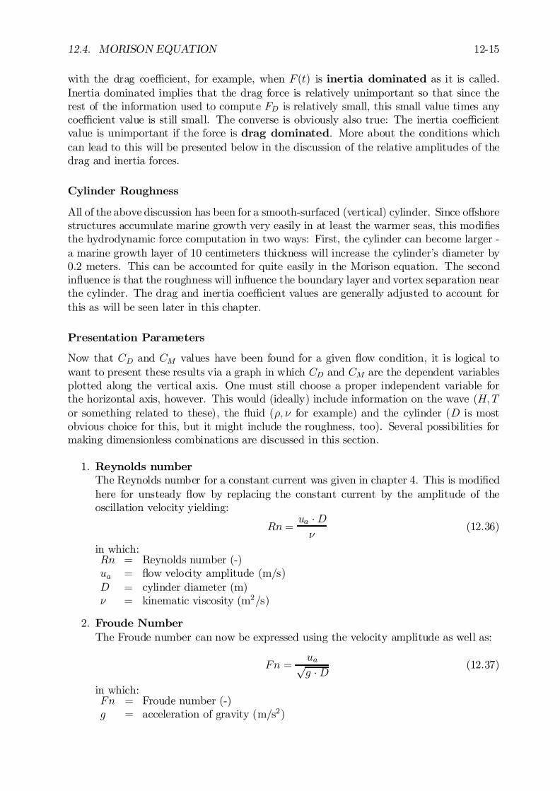
12.4. MORISON EQUATION 12-15
with the drag coe¢cient, for example, when F (t) is inertia dominated as it is called.Inertia dominated implies that the drag force is relatively unimportant so that since therest of the information used to compute FD is relatively small, this small value times anycoe¢cient value is still small. The converse is obviously also true: The inertia coe¢cientvalue is unimportant if the force is drag dominated. More about the conditions whichcan lead to this will be presented below in the discussion of the relative amplitudes of thedrag and inertia forces.
Cylinder Roughness
All of the above discussion has been for a smooth-surfaced (vertical) cylinder. Since o¤shorestructures accumulate marine growth very easily in at least the warmer seas, this modi…esthe hydrodynamic force computation in two ways: First, the cylinder can become larger -a marine growth layer of 10 centimeters thickness will increase the cylinder’s diameter by0.2 meters. This can be accounted for quite easily in the Morison equation. The secondin‡uence is that the roughness will in‡uence the boundary layer and vortex separation nearthe cylinder. The drag and inertia coe¢cient values are generally adjusted to account forthis as will be seen later in this chapter.
Presentation Parameters
Now that CD and CM values have been found for a given ‡ow condition, it is logical towant to present these results via a graph in which CD and CM are the dependent variablesplotted along the vertical axis. One must still choose a proper independent variable forthe horizontal axis, however. This would (ideally) include information on the wave (H;Tor something related to these), the ‡uid (½; º for example) and the cylinder (D is mostobvious choice for this, but it might include the roughness, too). Several possibilities formaking dimensionless combinations are discussed in this section.
1. Reynolds numberThe Reynolds number for a constant current was given in chapter 4. This is modi…edhere for unsteady ‡ow by replacing the constant current by the amplitude of theoscillation velocity yielding:
Rn =ua ¢Dº
(12.36)
in which:Rn = Reynolds number (-)ua = ‡ow velocity amplitude (m/s)D = cylinder diameter (m)º = kinematic viscosity (m2/s)
2. Froude NumberThe Froude number can now be expressed using the velocity amplitude as well as:
Fn =uapg ¢D (12.37)
in which:Fn = Froude number (-)g = acceleration of gravity (m/s2)
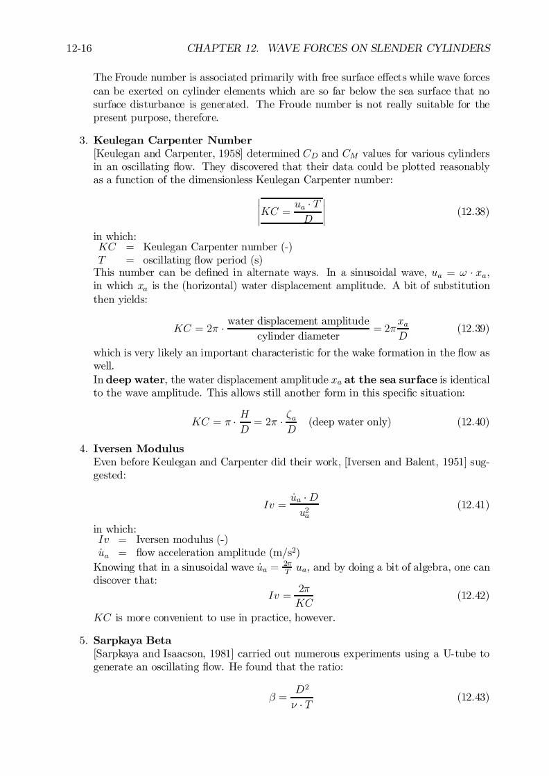
12-16 CHAPTER 12. WAVE FORCES ON SLENDER CYLINDERS
The Froude number is associated primarily with free surface e¤ects while wave forcescan be exerted on cylinder elements which are so far below the sea surface that nosurface disturbance is generated. The Froude number is not really suitable for thepresent purpose, therefore.
3. Keulegan Carpenter Number[Keulegan and Carpenter, 1958] determined CD and CM values for various cylindersin an oscillating ‡ow. They discovered that their data could be plotted reasonablyas a function of the dimensionless Keulegan Carpenter number:
¯¯KC = ua ¢ T
D
¯¯ (12.38)
in which:KC = Keulegan Carpenter number (-)T = oscillating ‡ow period (s)
This number can be de…ned in alternate ways. In a sinusoidal wave, ua = ! ¢ xa,in which xa is the (horizontal) water displacement amplitude. A bit of substitutionthen yields:
KC = 2¼ ¢ water displacement amplitudecylinder diameter
= 2¼xaD
(12.39)
which is very likely an important characteristic for the wake formation in the ‡ow aswell.In deep water, the water displacement amplitude xa at the sea surface is identicalto the wave amplitude. This allows still another form in this speci…c situation:
KC = ¼ ¢ HD= 2¼ ¢ ³a
D(deep water only) (12.40)
4. Iversen ModulusEven before Keulegan and Carpenter did their work, [Iversen and Balent, 1951] sug-gested:
Iv =_ua ¢Du2a
(12.41)
in which:Iv = Iversen modulus (-)_ua = ‡ow acceleration amplitude (m/s2)
Knowing that in a sinusoidal wave _ua = 2¼T ua; and by doing a bit of algebra, one can
discover that:Iv =
2¼
KC(12.42)
KC is more convenient to use in practice, however.
5. Sarpkaya Beta[Sarpkaya and Isaacson, 1981] carried out numerous experiments using a U-tube togenerate an oscillating ‡ow. He found that the ratio:
¯ =D2
º ¢ T (12.43)
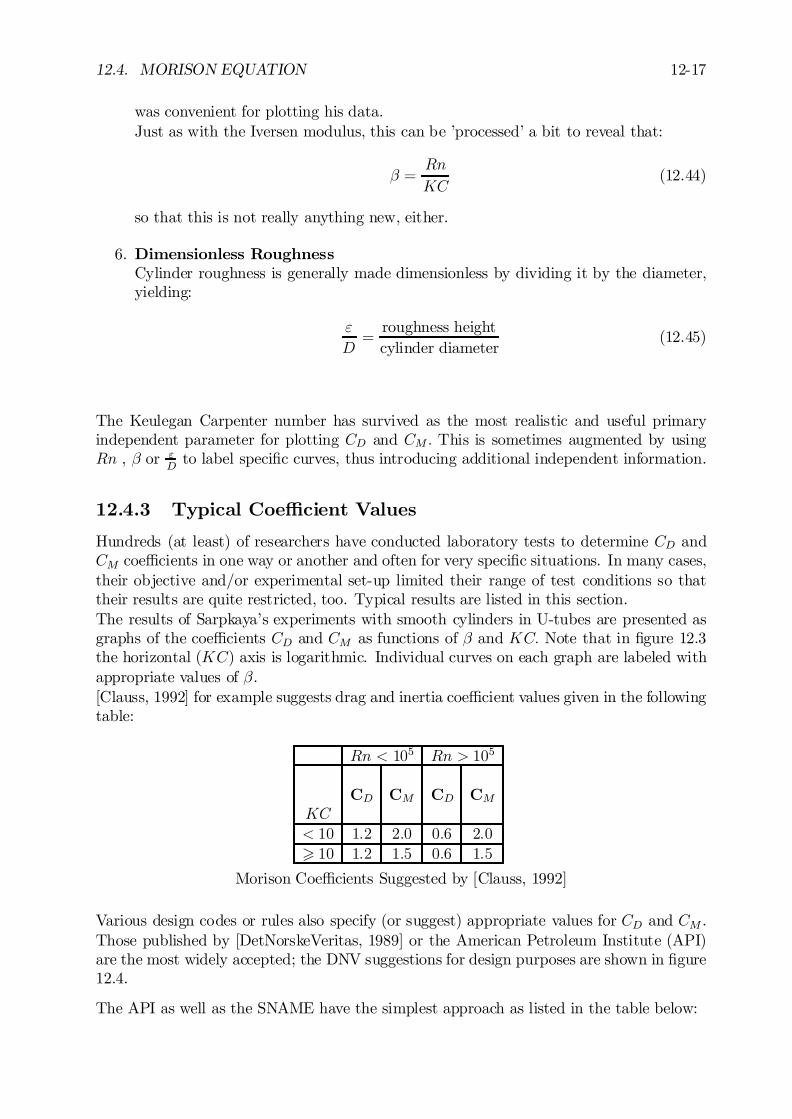
12.4. MORISON EQUATION 12-17
was convenient for plotting his data.Just as with the Iversen modulus, this can be ’processed’ a bit to reveal that:
¯ =Rn
KC(12.44)
so that this is not really anything new, either.
6. Dimensionless RoughnessCylinder roughness is generally made dimensionless by dividing it by the diameter,yielding:
"
D=
roughness heightcylinder diameter
(12.45)
The Keulegan Carpenter number has survived as the most realistic and useful primaryindependent parameter for plotting CD and CM : This is sometimes augmented by usingRn , ¯ or "
Dto label speci…c curves, thus introducing additional independent information.
12.4.3 Typical Coe¢cient Values
Hundreds (at least) of researchers have conducted laboratory tests to determine CD andCM coe¢cients in one way or another and often for very speci…c situations. In many cases,their objective and/or experimental set-up limited their range of test conditions so thattheir results are quite restricted, too. Typical results are listed in this section.The results of Sarpkaya’s experiments with smooth cylinders in U-tubes are presented asgraphs of the coe¢cients CD and CM as functions of ¯ and KC: Note that in …gure 12.3the horizontal (KC) axis is logarithmic. Individual curves on each graph are labeled withappropriate values of ¯.[Clauss, 1992] for example suggests drag and inertia coe¢cient values given in the followingtable:
Rn < 105 Rn > 105
CD CM CD CMKC< 10 1:2 2:0 0:6 2:0> 10 1:2 1:5 0:6 1:5
Morison Coe¢cients Suggested by [Clauss, 1992]
Various design codes or rules also specify (or suggest) appropriate values for CD and CM .Those published by [DetNorskeVeritas, 1989] or the American Petroleum Institute (API)are the most widely accepted; the DNV suggestions for design purposes are shown in …gure12.4.
The API as well as the SNAME have the simplest approach as listed in the table below:
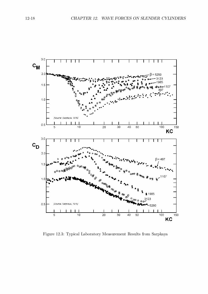
12-18 CHAPTER 12. WAVE FORCES ON SLENDER CYLINDERS
Figure 12.3: Typical Laboratory Measurement Results from Sarpkaya
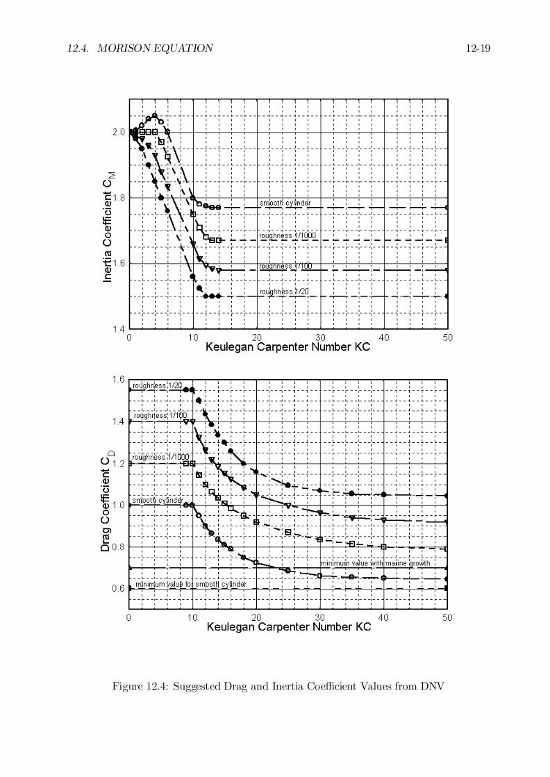
12.4. MORISON EQUATION 12-19
Figure 12.4: Suggested Drag and Inertia Coe¢cient Values from DNV

12-20 CHAPTER 12. WAVE FORCES ON SLENDER CYLINDERS
Smooth Rough
CD CM CD CMAPI 0:65 1:6 1:05 1:2
SNAME 0:65 2:0 1:0 1:8
The following observations can be made from the above information:- For low values of KC, the inertia coe¢cient CM is almost equal to its theoretical value
of 2 - at least if the KC value is used as a selection parameter. Also, one can noticethat the drag coe¢cient CD generally increases or stays rather constant till a valueof KC near 10 is reached.
- One sees as well from …gure 12.3 that the CD value gets lower as ¯ increases. This isjust the opposite of the trend observed with CM :
- Comparison of Sarpkaya’s curves (…gure 12.3) with those from DNV (…gure 12.4) showthat there can be quite some discrepancy in the value of CD or CM to choose.
- The DNV curves (…gure 12.4) as well as the other design and assessment codes includeroughness - that can easily result from marine growth, especially near the sea surface.The roughness in …gure 12.4 is an ²
D ratio.
- The API and SNAME recommendations seem rather simple in that they neglect theKC number; Clauss adds that e¤ect, but in a more simple way that suggested byDNV.
Comparisons
Examination and comparison of the various drag and inertia coe¢cient values presentedabove shows that there is little agreement on exact values. This is true for smooth cylindervalues and even more so when a rough cylinder is involved. Di¤erences of up to roughly40% can be found when comparing the drag or inertia coe¢cients suggested by the varioussources for a speci…c ‡ow situation.This direct comparison of coe¢cient values can be misleading, however. In some cases a lowdrag coe¢cient value can be at least partially compensated by a larger inertia coe¢cient.After choosing a typical cylinder diameter and wave conditions, one can select appropriatecoe¢cients from each of the sources and compute the actual maximum force per unit lengthupon which to base a comparison. Such an exercise can still lead to di¤erences of up toabout 30%. Luckily for survival design of o¤shore structures, the di¤erences found forextreme wave conditions are generally less than this!Even this comparison need not be correct. The ’purest’ approach is to select a typicalstructure, and place it (in one’s mind) at a given location in the sea. Given this, oneshould follow the entire procedure (given in each particular design or analysis code) toselect wave and current conditions and to translate these into forces on that structure.These resulting forces should be compared. Carrying out such a comparison operation isbeyond the scope of this text, however.One additional discovery that one will make when computing forces under …eld conditionsis that Sarpkaya’s data is a bit restricted for this. Indeed, the Reynolds numbers - neededfor his ¯ parameter - are much too low in nearly all laboratory situations.
12.4. MORISON EQUATION 12-21
12.4.4 Inertia or Drag Dominance
Now that CD and CM values have been presented, one should further re‡ect upon their useand importance. The Keulegan Carpenter number can be a very important parameter forthis. Indeed, it can be used as an indication of the relative importance of drag versus inertiaforces in a particular situation. To prove this, one must work out the ratio of the amplitudesof the drag and inertia forces. The 90± phase di¤erence between the force components iscompletely neglected now; only the force component amplitudes are compared.
FdragaFinertiaa
=12 ½ CD D ua juaj¼4½ CM D2 ! ua
=2 CD juaj¼ CM D !
(12.46)
Note that the maximum value of juaj is the same as that of ua.Since ! = 2¼=T; then this can be reduced a bit to:
FdragaFinertiaa
=1
¼2¢ CDCM
¢ ua ¢ TD
=1
¼2¢ CDCM
¢KC (12.47)
Since 1=¼2 ¼ 1=10 and the value of CD is often a bit more than half the CM value, thetwo force component amplitudes are about equal when KC is in the range of roughly 15to 20:Remembering the earlier de…nition of KC from equation 12.39:
KC =2¼ xaD
(12.48)
then this means that xa=D will be about 3; this is big enough to generate a very respectableset of vortices.
The Morison equation includes a nonlinear (quadratic drag) term which is 90± out of phasewith the inertia force. Many o¤shore engineers want to avoid using the entire Morisonequation (and the quadratic drag computation especially) unless it is absolutely necessary.It would be convenient to have a simple way to justify neglecting either the drag term orthe inertia term in that equation. The Keulegan Carpenter number is an excellent helpwith this:
² For low values of KC (KC < 3), the inertia force is dominant. The ‡ow ’does nottravel far enough’ relative to the cylinder diameter to generate much of a boundarylayer not to mention vortices; potential ‡ow theory is still applicable. Drag cansimply be neglected.
² For the next range until drag becomes signi…cant (3 < KC < 15); one will oftenlinearize the drag as has been explained earlier in this chapter.
² There is a range of KC (15 < KC < 45) in which one cannot really avoid using thefull Morison equation with its nonlinear drag.
12-22 CHAPTER 12. WAVE FORCES ON SLENDER CYLINDERS
² For high values of KC (KC > 45), the drag force is dominant. The vortexshedding frequency becomes high compared to the wave frequency so the ‡ow tendsto behave more and more like a uniform ‡ow. Inertia can be neglected. Indeed,the limit KC ! 1 corresponds to a constant current.
12.5 Forces on A Fixed Cylinder in Various Flows
This section describes the forces acting on a …xed cylinder in currents and/or waves. Whileparts of it may seem like repetition of earlier work, its objective is to clarify the underlyingprinciples.
12.5.1 Current Alone
A …xed cylinder in a current alone will experience only a quadratic drag force (per unitlength) as already indicated in chapter 4. This force is assumed to be caused by the ‡owcomponent:
Up = U sin·
acting perpendicular to the cylinder axis so that the force can be expressed as:
Fc =1
2½ U2D CD sin
2 · (12.49)
In these equations:
U = Total velocity vector (m/s)Up = Perpendicular velocity component (m/s)CD = Drag coe¢cient for constant current (-)· = Cone angle between the velocity vector, U;
and the cylinder axis.Fc = Current force per unit cylinder length (N/m)
See …gure 12.5 for a sketch showing the cone angle. The force, Fc; will act in the directionof Up of course; this is perpendicular to the cylinder axis and in the plane de…ned by thecylinder axis and the approaching velocity vector, U:Note that only the so-called cone angle, ·; is important in this computation. This issu¢cient to describe the orientation of the cylinder relative to the current vector. It makesno di¤erence whether the cylinder is in a vertical, horizontal or any other plane; it is onlythe angle between the cylinder axis and total velocity vector which is important. (Thiswill be generalized to include inertia forces in waves below.)
12.5.2 Waves Alone
The time dependent ‡ow associated with waves requires the inclusion of inertia force com-ponents into a force computation. Indeed, the basic Morison equation - derived for a unitlength of a …xed, vertical cylinder in waves is re-stated here for reference:
¯¯F = 1
4¼ ½ D2 CM _u(t) +
1
2½ CD D u(t) ju(t)j
¯¯ (12.50)
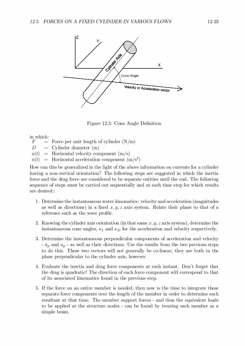
12.5. FORCES ON A FIXED CYLINDER IN VARIOUS FLOWS 12-23
Figure 12.5: Cone Angle De…nition
in which:F = Force per unit length of cylinder (N/m)D = Cylinder diameter (m)u(t) = Horizontal velocity component (m/s)_u(t) = Horizontal acceleration component (m/s2)
How can this be generalized in the light of the above information on currents for a cylinderhaving a non-vertical orientation? The following steps are suggested in which the inertiaforce and the drag force are considered to be separate entities until the end. The followingsequence of steps must be carried out sequentially and at each time step for which resultsare desired::
1. Determine the instantaneous water kinematics: velocity and acceleration (magnitudesas well as directions) in a …xed x; y; z axis system. Relate their phase to that of areference such as the wave pro…le.
2. Knowing the cylinder axis orientation (in that same x; y; z axis system), determine theinstantaneous cone angles, ·I and ·D for the acceleration and velocity respectively.
3. Determine the instantaneous perpendicular components of acceleration and velocity- _up and up - as well as their directions. Use the results from the two previous stepsto do this. These two vectors will not generally be co-linear; they are both in theplane perpendicular to the cylinder axis, however.
4. Evaluate the inertia and drag force components at each instant. Don’t forget thatthe drag is quadratic! The direction of each force component will correspond to thatof its associated kinematics found in the previous step.
5. If the force on an entire member is needed, then now is the time to integrate theseseparate force components over the length of the member in order to determine eachresultant at that time. The member support forces - and thus the equivalent loadsto be applied at the structure nodes - can be found by treating each member as asimple beam.
12-24 CHAPTER 12. WAVE FORCES ON SLENDER CYLINDERS
6. Since the inertia and drag force components are not generally colinear, they canbe combined (if desired) via vector addition to yield the resulting force magnitudeand its direction (still in a plane perpendicular to the cylinder axis). This step isnot absolutely necessary for the computation of resulting forces on a large structure,however.
Note that these …ve or six steps must be repeated at each instant in time. These steps arenot di¢cult in principle, but very careful bookkeeping is essential!In many simple cases, each of the quantities needed for this methodology will be express-ible in terms of nicely behaved and convenient functions so that the resulting force can bedescribed as one or another continuous time function. On the other hand, if the wave isirregular and thus composed of many frequency and direction components, then the neces-sary bookkeeping becomes too cumbersome for a hand calculation. The only requirementfor the force computation is that the water acceleration and velocity be known at any time.
Special Orientations
One can check his or her understanding of the above by evaluating the forces acting ontwo special cases of a horizontal cylinder in a regular wave. These are in addition to thevertical cylinder used during the Morison equation derivation.If the horizontal cylinder segment is oriented with its axis parallel to the directionof wave propagation (and thus perpendicular to the wave crests), then it will experiencea vertical force which has a time trace which looks much like that for a vertical cylinder -see …gure 12.2. This force record will be shifted 90± in phase relative to a similar recordfor a vertical cylinder, however. The relative phases of the resulting drag and inertial forcecomponents on consecutive segments of the cylinder will correspond - with some constantshift - to that of the wave pro…le on the sea surface.The second case has the horizontal cylinder turned parallel to the wave crests (andthus perpendicular to the direction of wave propagation). If the cylinder is situated in adeep water wave (in which the horizontal and vertical kinematic components have the samemagnitudes) then one will …nd a resultant force of constant magnitude which sweeps aroundthe cylinder once per wave period. It may seem strange, but the horizontal component ofthis force will have a purely sinusoidal form (except for a possible phase shift) independentof the fact that quadratic drag is involved. Force components on consecutive segments ofthis cylinder will have identical phases in this case as compared to the previous one.
12.5.3 Currents plus Waves
It is generally accepted practice to vectorially superpose the current velocity on the velocityresulting from the waves before calculating the drag force. In a general case the wave andcurrent directions will not be co-linear making a vector sum necessary. Once this has beencarried out, however, one simply has to use the sequential steps given above to determinethe resulting force at any instant.Why is it not acceptable to compute the wave force and the current force separately? Thecurrent has no e¤ect at all on the ‡ow accelerations so that the inertia force is unchangedby the current. The di¢culty lies with the quadratic drag force. Since:
U2p + u2p < (Up + up)
2 (12.51)
12.6. FORCES ON AN OSCILLATING CYLINDER IN VARIOUS FLOWS 12-25
then a segregated treatment of the current drag and wave drag - which are superposed onlyat the end of the computation - will lead to an underestimation of the forces involved.
12.6 Forces on An Oscillating Cylinder in Various Flows
Now that the hydrodynamic interaction of a …xed cylinder in a variety of ‡ows has beenexplained, it is appropriate to discuss the hydrodynamic interaction of a moving cylinder- again in a variety of ‡ow conditions.A distinction will now have to be made between the (external) force exerted by the cylinderon the surrounding water and the (internal, structural) force needed to cause the cylinder(segment) to oscillate. In general, the internal force will often be one that is measured -especially in a laboratory setting. This force includes the external hydrodynamic force butalso includes a force needed to accelerate the cylinder itself. Also, one should remember thatthe hydrodynamic interaction force components will generally be in a direction opposite tothe actual velocity and acceleration of the cylinder.
12.6.1 Still Water
As indicated much earlier in this chapter, the Froude-Krilov force will be absent sincethere are no ambient pressure gradients in water which is at rest. The inertia force willbe associated with a Ca value and there will be a drag force - associated with CD as well.Analogous to the assumption made for a …xed cylinder, these forces will be associated withthe cylinder kinematics components (velocity and acceleration) which are perpendicular tothe cylinder’s axis.The …ve steps used for determining the forces on a …xed cylinder can used here too, albeitthat the kinematics now is that of the cylinder instead of the water.
12.6.2 Current Alone
This interaction situation has already been discussed to some extent in chapter 4. Oneshould remember that the direction of cylinder oscillation and the current direction maybe quite di¤erent. Indeed, a vortex-induced vibration usually has its largest componentmore or less perpendicular to the current direction. This results from the lift force - themost important dynamic force in this ‡ow situation - which was discussed in chapter 4.The drag component of the hydrodynamic interaction was quite well described in section6 of that chapter too; there is no need to repeat that here.Inertia forces will - in principle - now be present, too. They will be associated with aCa value since there is still no ambient time-dependent pressure gradient. These forceswill be opposite to the acceleration component which results exclusively from the cylinderoscillation in this case.In many realistic cases the approaching ‡ow velocity will be considerably larger than thecylinder’s oscillation velocity. Also, since most oscillating cylinders are rather slender (anumbilical cable to a ROV is an excellent example) the KC number will be large so thatinertia forces will be small anyway. In many practical situations, then, one considers onlya drag force as if it were exerted on a …xed cylinder. The drag coe¢cient is sometimes abit larger to account for the wider wake resulting from the cylinder oscillation.

12-26 CHAPTER 12. WAVE FORCES ON SLENDER CYLINDERS
12.6.3 Waves Alone
The inertia and drag forces are treated entirely separately here for clarity.
Inertia Forces
Waves will contribute both a Froude-Krilov force (from the ambient, time-dependent pres-sure gradient) as well as a disturbance force from the encounter with the solid cylinder.The cylinder oscillation, on the other hand, plays no role in the Froude-Krilov force butit does contribute to the disturbance term. (It is implicitly assumed here that the motionof the cylinder is small relative to the wave length so that no phase changes result fromthis displacement. It is hard to conceive of a practical situation for which this assumptiondoes not hold.) When one keeps in mind that the direction of cylinder oscillation need notcoincide with the wave direction, then careful bookkeeping is called for.One …nds the following inertia terms in the equation of motion:
M ÄX(t)¯ CM MD _up(t)¡ Ca MDÄX(t) (12.52)
in which:M = Mass of the cylinder segment (kg/m)MD = Displaced water mass = ¼
4D2½ (kg/m)
_up(t) = Perpendicular acceleration component from the waves (m/s2)ÄX(t) = Cylinder acceleration (m/s2)
The symbol ¯ has been used to segregate terms from the left hand side of the full equationof motion from those on the right. Since only selected terms are included, true equalitycannot be guaranteed. The above relationship can be re-arranged by splitting the waveforce term into its two components so that:
M ÄX(t)¯ 1 MD _up(t) + Ca MD _up(t) ¡ Ca MDÄX(t) (12.53)
If the cylinder acceleration corresponds exactly - in both magnitude and direction - to thatof the waves, then the last two terms in this latter equation cancel. This is logical; thereis then no disturbance at all and only the Froude-Krilov force remains.In the more general case, all three hydrodynamic force components in equation 12.53 willbe present. It is often convenient to move all the force terms involving the cylinder motionto the left hand side of the equation so that it becomes:
(M +Ca MD) ÄX(t) ¯CM MD _up(t) (12.54)
This isolates the (unknown) cylinder motion on the left hand side of the equation andplaces the time-dependent external exciting force on the right. This right hand side canbe evaluated (without knowing the cylinder motion) as a pure time function before thedi¤erential equation of the cylinder motion is evaluated.
Drag Forces
Drag forces result from the ‡ow disturbance and wake near the cylinder. Two quite dif-ferent approaches to the description of hydrodynamic drag are used. They are discussedseparately here.
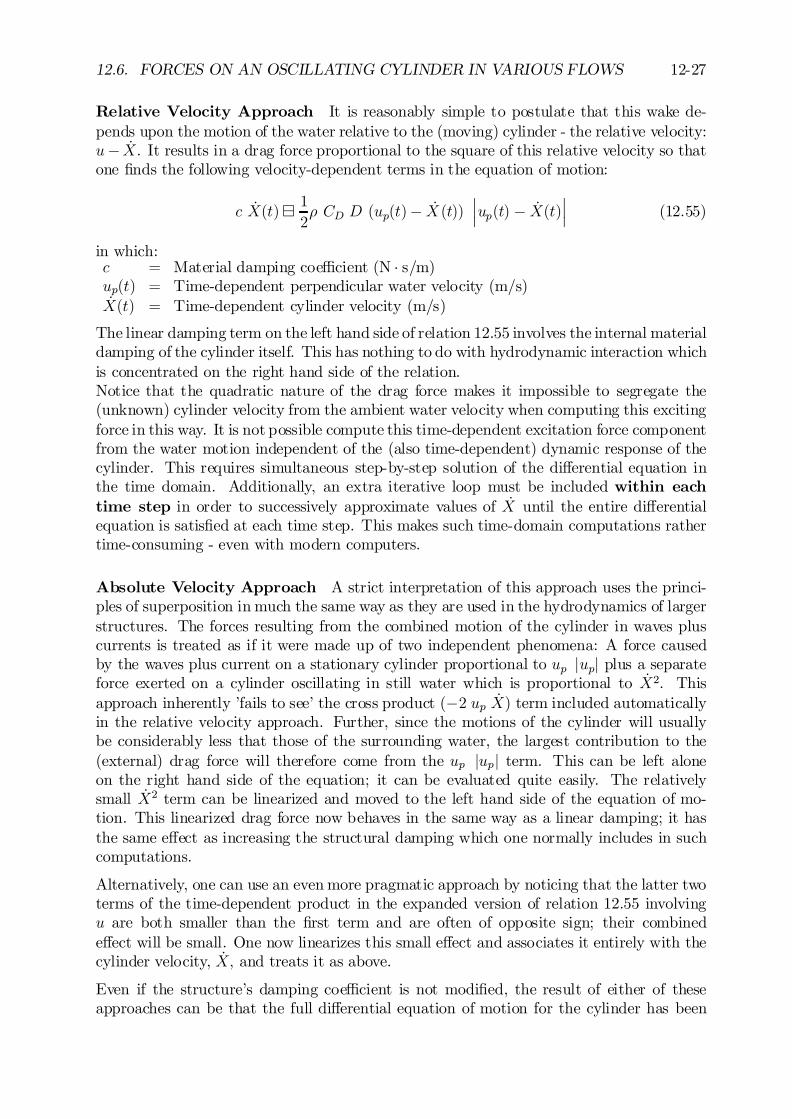
12.6. FORCES ON AN OSCILLATING CYLINDER IN VARIOUS FLOWS 12-27
Relative Velocity Approach It is reasonably simple to postulate that this wake de-pends upon the motion of the water relative to the (moving) cylinder - the relative velocity:u¡ _X. It results in a drag force proportional to the square of this relative velocity so thatone …nds the following velocity-dependent terms in the equation of motion:
c _X(t)¯ 12½ CD D (up(t)¡ _X (t))
¯¯up(t) ¡ _X(t)
¯¯ (12.55)
in which:c = Material damping coe¢cient (N ¢ s/m)up(t) = Time-dependent perpendicular water velocity (m/s)_X(t) = Time-dependent cylinder velocity (m/s)
The linear damping term on the left hand side of relation 12.55 involves the internal materialdamping of the cylinder itself. This has nothing to do with hydrodynamic interaction whichis concentrated on the right hand side of the relation.Notice that the quadratic nature of the drag force makes it impossible to segregate the(unknown) cylinder velocity from the ambient water velocity when computing this excitingforce in this way. It is not possible compute this time-dependent excitation force componentfrom the water motion independent of the (also time-dependent) dynamic response of thecylinder. This requires simultaneous step-by-step solution of the di¤erential equation inthe time domain. Additionally, an extra iterative loop must be included within eachtime step in order to successively approximate values of _X until the entire di¤erentialequation is satis…ed at each time step. This makes such time-domain computations rathertime-consuming - even with modern computers.
Absolute Velocity Approach A strict interpretation of this approach uses the princi-ples of superposition in much the same way as they are used in the hydrodynamics of largerstructures. The forces resulting from the combined motion of the cylinder in waves pluscurrents is treated as if it were made up of two independent phenomena: A force causedby the waves plus current on a stationary cylinder proportional to up jupj plus a separateforce exerted on a cylinder oscillating in still water which is proportional to _X2. Thisapproach inherently ’fails to see’ the cross product (¡2 up _X) term included automaticallyin the relative velocity approach. Further, since the motions of the cylinder will usuallybe considerably less that those of the surrounding water, the largest contribution to the(external) drag force will therefore come from the up jupj term. This can be left aloneon the right hand side of the equation; it can be evaluated quite easily. The relativelysmall _X2 term can be linearized and moved to the left hand side of the equation of mo-tion. This linearized drag force now behaves in the same way as a linear damping; it hasthe same e¤ect as increasing the structural damping which one normally includes in suchcomputations.
Alternatively, one can use an even more pragmatic approach by noticing that the latter twoterms of the time-dependent product in the expanded version of relation 12.55 involvingu are both smaller than the …rst term and are often of opposite sign; their combinede¤ect will be small. One now linearizes this small e¤ect and associates it entirely with thecylinder velocity, _X; and treats it as above.
Even if the structure’s damping coe¢cient is not modi…ed, the result of either of theseapproaches can be that the full di¤erential equation of motion for the cylinder has been
12-28 CHAPTER 12. WAVE FORCES ON SLENDER CYLINDERS
linearized and that the wave-caused excitation force has been isolated on its right handside. Each motion is treated as if it is in a …xed axis system. It is for this reason that thisapproach is often referred to as the absolute motion approach.
Comparison Designers tend to be conservative in practice. As a result of this, they tendnot to modify the linearized damping when using the absolute motion approach. Since adynamic system with a lower damping will often have a larger response, the absolute motionapproach most usually leads to higher predicted structural responses (internal stresses oreven displacements, for example) than does the relative velocity approach. This is indeed astrong motivation to use the absolute velocity approach when evaluating the performanceof a proposed design. The additional advantage of having a straightforward and simplecomputational procedure comes as an added bonus.
12.6.4 Currents Plus Waves
Just as with the …xed cylinder, all hydrodynamic velocity components are generally super-posed before starting a force computation. Once this has been done, the further treatmentis identical to that for an oscillating cylinder in waves alone as discussed above.
12.7 Force Integration over A Structure
The discussion above has concentrated on the forces on a unit length of cylinder or at leastno more than a single member of a large truss structure. It is now time to integrate theseforces over the length of the cylinder in order to determine loads which are relevant forstructural analysis and design evaluation.Since many space truss analysis computer programs work with externally applied jointloads, the goal should be to transform the distributed hydrodynamic load on each memberof the structure to equivalent concentrated loads at the structure’s nodes. Generally, thisprocedure will have to be followed during a whole series of discrete time steps in order togenerate time-dependent loadings which may be needed for a dynamic analysis.Many computer programs for this purpose work somewhat as follows:As preparation,
² The nodes of the structure are numbered sequentially.
² Each node is assigned a set of X;Y; Z coordinates corresponding to the intersectionpoint of the member axes at that joint. (Any member eccentricity at the joint isneglected in the hydromechanics.)
² Each member is speci…ed by its diameter and the numbers of the two nodes which itjoins. Each member’s geometric position and length is now de…ned.
Once this has been completed the following steps will be carried out for the dynamic loadsat each desired time step:
1. The water kinematics - both combined velocities and accelerations - will be computedat each node location. It makes no di¤erence now whether the waves are regular orirregular; there can even be directional spreading or additional currents involved.

12.7. FORCE INTEGRATION OVER A STRUCTURE 12-29
The result in all cases is known water kinematics at each node and at every chosentime.
2. If a dynamic calculation is included, and relative velocity drag is used, then thestructure’s velocity and acceleration at each node will have to be estimated as well.This is usually done by incrementally integrating the structure’s equations of motionby working from the previous time step.
3. The results of the above two steps along with the known geometry allow the com-putation of the force per unit length (for inertia and drag forces separately) at eachend of each member. These load intensities will have to be computed separately foreach member and at each of its end joints.
4. Most programs now consider each member to be a simple beam carrying a distributedload which is assumed to vary linearly from one end to the other. Note that both theintensity of the loading as well as the vector direction of the loading (about the axisof the cylinder) may vary along its length. (Direction variation can be present whenthe waves and current are not co-linear. It is also present when wave directionalspreading is involved.)
5. Basic mechanics yields the two reaction force components (relative to each member’saxis!) at each of its ends.
6. It is now only a matter of bookkeeping to transform these individual member reactionforces into equivalent X;Y; Z force components at each joint.
7. The above X;Y; Z components at each joint are summed to determine the totalequivalent applied dynamic load at that joint at the chosen moment. This is thedesired result.
8. If relative velocity hydrodynamics is being used this result must be checked. Theequations of motion of the structure must be integrated now to determine its newvelocity and acceleration at the end of the time step. If these values do no correspond(within a chosen tolerance) with those estimated in step 2, then the above stepsmust be repeated for another iteration cycle - within this same time step - until theestimated and computed values appropriately coincide.
It is the extra iteration loop discussed in the last of the above steps that makes the rel-ative velocity approach to hydromechanics so computationally ine¢cient relative to otherapproaches.Constant static loads, such as member weight and buoyant forces, can be included in theabove computation, but can be computed more e¢ciently separately before starting on thedynamic computations. The computation principle is analogous to that for the dynamicloads, by the way.

12-30 CHAPTER 12. WAVE FORCES ON SLENDER CYLINDERS
.
Chapter 13
SURVIVAL LOADS ON TOWERSTRUCTURES
13.1 Introduction
Chapter 12 has discussed how to compute the hydrodynamic forces on an element (ofunit length) of a single (slender) cylinder; a simpli…ed means of estimating the largesthydrodynamic forces on an o¤shore tower structure will be handled in this chapter.Figure 13.1 shows an isometric drawing of one of the larger o¤shore structures. Theannotations in that …gure will become clear in the course of this chapter.Some refer to such a structure as a space frame, others see it as a space truss, some justcall it a tower. The terms ’frame’ and ’truss’ have quite di¤erent structural engineeringconnotations which are not at all relevant to the hydrodynamic discussion in this chapter.Another structural distinction is that a jacket is supported from the top by piles driventhrough its legs while a tower is generally supported from below by piles driven throughsleeves - usually at the sea bed. This distinction is also irrelevant for the hydrodynamicsbeing discussed here; the term tower will be used more generically in this chapter to referto any three-dimensional structure made up from slender elements.Imagine the bookkeeping and computational e¤ort needed to compute the total hydro-dynamic forces on the structure shown in …gure 13.1 if this were to be done using theelemental methods of chapter 12. Such a rigorous computation for a ’real’ tower structure(with all its members: chords, braces, risers, etc.) is a very cumbersome undertaking,indeed.Many design engineers have no need for the computational accuracy suggested by a detailedschematization of such a complex o¤shore structure - at least not during the preliminarydesign phase. Instead, one more often needs a fast method of making a rough and preferablyconservative estimate of the hydrodynamic forces on a complex o¤shore structure. Sucha method can serve two purposes: Give a rough estimate for preliminary design or assurethat a detailed model is not making a major error. The objective of this chapter is tooutline a ’quick and dirty’ method to estimate the horizontal loads on a tower structure.These loads generally yield the largest overall bending moments in the structure and thusaxial leg forces as well as the largest horizontal shear forces. These forces and moments arealso important for the foundation design. Maximum in-service bracing loads result from
0J.M.J. Journée and W.W. Massie, ”OFFSHORE HYDROMECHANICS”, First Edition, January 2001,Delft University of Technology. For updates see web site: http://www.shipmotions.nl.
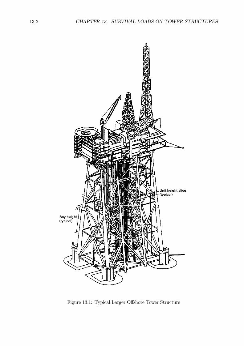
13-2 CHAPTER 13. SURVIVAL LOADS ON TOWER STRUCTURES
Figure 13.1: Typical Larger O¤shore Tower Structure
13.2. ENVIRONMENTAL CONDITIONS TO CHOOSE 13-3
the horizontal wave and current loads as well.
13.1.1 Method Requirements
The results obtained with any approximation need not be exact - especially if one canreasonably predict whether the ’real’ loads will be smaller (or larger) than the estimates.Generally - and for preliminary design in particular - it is handy if the hydrodynamic loadsresulting from the approximation are larger than those which would follow from a moresophisticated analysis.When a preliminary design is based upon loads which are overestimated, it is most likelythat the resulting structure will be ’over-designed’; it will be a bit too big, or heavy, orstrong and thus probably too costly. Given this fact, then one would not expect the costsof a structure resulting from a more detailed design to come out too high. Said in anotherway, if the preliminary design survives an economic analysis, then the …nal design has agood chance of surviving this too - at least to the extent that its total cost is determined byhydrodynamics. An additional factor in practice is that topsides tend to become heavier(as more equipment is added) rather than lighter during the design process. (Whether onelikes it or not, topside structures usually tend to get larger and heavier in the course oftheir detailed design. This can result from equipment or throughput changes as well asfrom modi…ed environmental or safety requirements.) To the extent that the tower designis dictated by topside weight (if the water is not all that deep depending upon the seaconditions), a bit of initial tower overdesign can prove to be handy during the later, moredetailed design analysis phase.The objective of this chapter, therefore, is to come up with a computational procedure toconservatively predict the hydrodynamic forces on a complex o¤shore tower structure.
13.1.2 Analysis Steps
Any hydrodynamic analysis of an o¤shore structure involves the following steps:1. Selection of environmental conditions (raw data).2. Schematization of the ambient hydrodynamics.3. Schematization of the structure.4. Computation of resulting (survival) forces and overturning moments.
These steps will be followed in the remainder of this chapter.
13.2 Environmental Conditions to Choose
Since one is looking for a maximum external load condition, it is common that this willbe caused by a maximum environmental input condition. (A signi…cant dynamic response- which via resonance can lead to enhanced internal loads - can lead to internal responsemaxima (leg forces, for example) which are caused by more moderate external sea condi-tions. This is not considered here; it is not that common with tower structures, anyway.)All of this means that extreme wind, wave and current conditions should be chosen forthis …rst design. Each of these involves at least two independent variables: Speed (in someform) and direction. All of environmental inputs can be represented as vectors, but theirscalar magnitudes and directions are discussed separately here.
13-4 CHAPTER 13. SURVIVAL LOADS ON TOWER STRUCTURES
Wind Speed
Wind loads on o¤shore structures often play a relatively minor role in comparison to thehydrodynamic loads. For an o¤shore wind turbine, even - on which one would expectto have a relatively high wind load - the wind load is seldom greater than the combinedwave and current load unless the structure is placed in water somewhat less than about 20meters deep (in the North Sea). This implies that the selection of design wind conditionsis often not all that important. When one does want to estimate wind loads, a maximumone-minute wind gust is often chosen. This wind speed is usually measured at a ’standard’elevation of 10 meters above the sea surface.
Current Speed
Maximum current speeds are usually chosen for survival design purposes as well. One couldselect a speed corresponding to a maximum spring tide current, for example. In some casesa velocity pro…le giving the current as a function of depth will be available, too. If not, itis of course conservative to assume that the maximum current acts over the entire depth.
Wave Height and Period
One should choose wave height and period values such that a maximum wave force oroverturning moment is obtained. A high wave is obviously needed. If one assumes thatthe worst part of a storm will have a duration of about 3 to 6 hours and that an extremewave - if seen as a single wave - will have a period of in the order of 15 to 20 seconds,then one can expect an exposure to something in the order of 1000 waves during the peakof the storm. The highest wave in a series of 1000 would have a chance of exceedance of11000: Substituting this in a Rayleigh wave height distribution yield a design wave height of1:86 times the design signi…cant wave height chosen. (If one works out these limits moreexactly, one should expect something more than 540 waves and less than 1440 of them;one thousand is pretty close to the average - by chance. If 1
540 and 11440 are used instead,
the wave height ratio is in the range 1.77 to 1.91; this makes no more than 5% di¤erence.)Selecting the shortest wave period consistent with the chosen wave height will yield max-imum water velocities and accelerations - at least near the water surface. On the otherhand, the hydrodynamics of waves with shorter periods ’die out’ faster at deeper locations;a proper balance must be found between these two requirements. Wave breaking will, ofcourse, put a lower limit on the wave period for a given wave height; a very high and veryshort wave will break so that one should also check any chosen combination of these to besure that the wave is not broken. The necessary relationships (for deep water and a quickestimate) include:
¸ = 1:56 ¢ T 2 andH
¸<1
7(13.1)
in which ¸ is the wave length (m), H is the wave height (m) and T is the wave period (s).The above relations - which come directly from regular wave theory of chapter 5 - are lessdependable for larger and irregular waves at sea, however.Since H will generally be rather large, ¸ will not be small, either. The signi…cance of thiswill show up below.
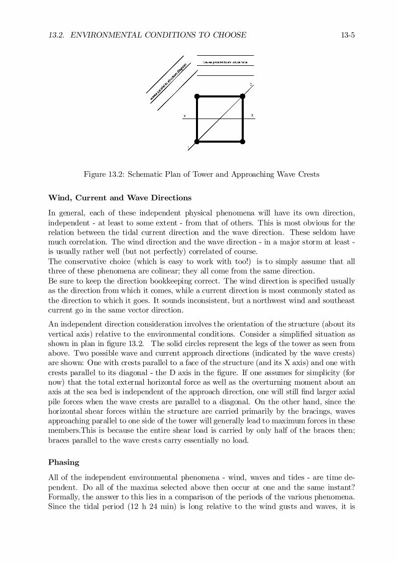
13.2. ENVIRONMENTAL CONDITIONS TO CHOOSE 13-5
Figure 13.2: Schematic Plan of Tower and Approaching Wave Crests
Wind, Current and Wave Directions
In general, each of these independent physical phenomena will have its own direction,independent - at least to some extent - from that of others. This is most obvious for therelation between the tidal current direction and the wave direction. These seldom havemuch correlation. The wind direction and the wave direction - in a major storm at least -is usually rather well (but not perfectly) correlated of course.The conservative choice (which is easy to work with too!) is to simply assume that allthree of these phenomena are colinear; they all come from the same direction.Be sure to keep the direction bookkeeping correct. The wind direction is speci…ed usuallyas the direction from which it comes, while a current direction is most commonly stated asthe direction to which it goes. It sounds inconsistent, but a northwest wind and southeastcurrent go in the same vector direction.
An independent direction consideration involves the orientation of the structure (about itsvertical axis) relative to the environmental conditions. Consider a simpli…ed situation asshown in plan in …gure 13.2. The solid circles represent the legs of the tower as seen fromabove. Two possible wave and current approach directions (indicated by the wave crests)are shown: One with crests parallel to a face of the structure (and its X axis) and one withcrests parallel to its diagonal - the D axis in the …gure. If one assumes for simplicity (fornow) that the total external horizontal force as well as the overturning moment about anaxis at the sea bed is independent of the approach direction, one will still …nd larger axialpile forces when the wave crests are parallel to a diagonal. On the other hand, since thehorizontal shear forces within the structure are carried primarily by the bracings, wavesapproaching parallel to one side of the tower will generally lead to maximum forces in thesemembers.This is because the entire shear load is carried by only half of the braces then;braces parallel to the wave crests carry essentially no load.
Phasing
All of the independent environmental phenomena - wind, waves and tides - are time de-pendent. Do all of the maxima selected above then occur at one and the same instant?Formally, the answer to this lies in a comparison of the periods of the various phenomena.Since the tidal period (12 h 24 min) is long relative to the wind gusts and waves, it is
13-6 CHAPTER 13. SURVIVAL LOADS ON TOWER STRUCTURES
almost certain that a high wave or strong wind gust can occur when the tidal current ishigh.Looking next at the wind gust relative to the wave, its duration (1 minute) would be afew wave periods long. Here, again, there is at least some …nite chance that a major wavepeak will coincide with this in time. On the other hand, many more waves will occur attimes when the design wind gust is not present!Of course, assuming that the maxima of wind, waves and current do occur simultaneouslywill lead to a conservative result; this is chosen here.
Implications
The choices made above already have signi…cant implications for the computations to becarried out. For example, the wave length, ¸ , chosen above will be rather large relative tothe horizontal dimensions of (most) o¤shore structures being considered. This means thatthere will be relatively little phase di¤erence between the ’upstream’ and ’downstream’sides of the entire structure at any instant in time.In chapter 12 the phase shift from one side to the other side (of a single cylinder) wasneglected. Now, with an extreme wave, the same reasoning is being applied to an en-tire tower structure. Since phase di¤erences only tend to reduce the horizontal loads onthe structure, neglecting these will be conservative. Additionally, neglecting this phasedi¤erence will simplify the formulation of the structural model enormously.Since the wave is relatively high, the Keulegan Carpenter number KC = ¼¢H
D(at the sea
surface and in deep water) will tend to be high as well. This indicates that the wave forceswill tend to be drag dominated - at least at the sea surface where they are largest.Note that if the structure is not in deep water, the actual KC value will be even higherthan that estimated above; this can be checked by using the complete equations - ratherthan deep water approximations - to describe the water motion. When the current is addedto the water velocity caused by the wave, then this drag dominance becomes even morepronounced, of course. In all cases, the water velocity will decrease with depth so that theKC value will decrease as well. One can expect the inertia force to increase in importanceas one moves down along the structure. A signi…cant current can prevent it from everplaying much role, however.Remember too from wave kinematics that the maximum horizontal water velocity in awave occurs under that wave crest or trough. The total resulting force (integrated overthe structure) will be greatest when the wave crest passes by, simply because more of thestructure is then exposed to the wave. Wave kinematics will have to be predicted over theentire height from the sea bed to the wave crest in order to carry out such a computation.
13.3 Ambient Flow Schematizations
This section discusses the numerical models needed to translate the raw data on environ-mental conditions into input data for a force model.
Wind
Wind velocity distributions have been discussed in chapter 4. If - as is standard meteoro-logical practice - the wind is given at a standard elevation of 10 meters above mean sea

13.3. AMBIENT FLOW SCHEMATIZATIONS 13-7
level, then wind speeds at other elevations are often predicted from this value by using:
Vtw(z)
Vtw(10)=
³ z10
´0:11(at sea) (13.2)
in which:
z = desired elevation (m)Vtw(z) = true wind speed at elevation z (m/s)Vtw(10) = true wind speed at 10 meters elevation (m/s)
The exponent 0:11 in equation 13.2 is for sea conditions only; see chapter 4.
Some designers often reason that since wind loads on many o¤shore structures are oftenrelatively unimportant and hydrodynamic loads tend to be over-estimated, they can justneglect wind loads altogether. This is certainly the very simplest approach that can bechosen. On the other hand, the wind load has the longest moment arm when one is studyingthe overturning moments about the structure’s base. It is best not to neglect them in theoverturning moment computation at least.
Waves
A maximum wave at sea results from the superposition of a large number of wave spectrumcomponents. The objective here is to replace this multi-component wave with a singleregular wave for computation purposes. Linear wave theory is certainly convenient forpredicting the water kinematics within such a wave, but it has one important drawback:It predicts water motions only in the zone below mean sea level. As has been indicatedabove, the water motions right up to the wave crest will have to be predicted. Methodsfor doing this have been given in chapter 5. Of these, the use of a constant velocity - thesame as the velocity at z = 0 - or Wheeler stretching are the most popular.Remember from chapter 5 that the (extreme) wave crest will be higher than H=2 abovethe still water level as well. A common rule of thumb is that:
³max = +2
3H and ³min = ¡1
3H (13.3)
With this, one can use either constant extension or Wheeler stretching along with thecomplete equations for the water motion in order to calculate the horizontal componentsof water particle acceleration and velocity at all elevations between the sea bed and wavecrest. All details of this can be found in chapter 5.
One should note the following about the waves formulas to be used:
1. If only a maximum velocity is needed, the time function in the wave can be neglected.2. Since the wave length is usually considerably larger than the horizontal dimensions
of the total structure being considered, the phase relation, kx can be dropped too.
3. If the wave crest is involved, then the maximum crest elevation will follow fromequation 13.3.
4. The full equations (and not deep or shallow water approximations) must be usedwhen evaluating the horizontal kinematics in the wave. This is then valid for anywater depth and at any point under a wave pro…le.
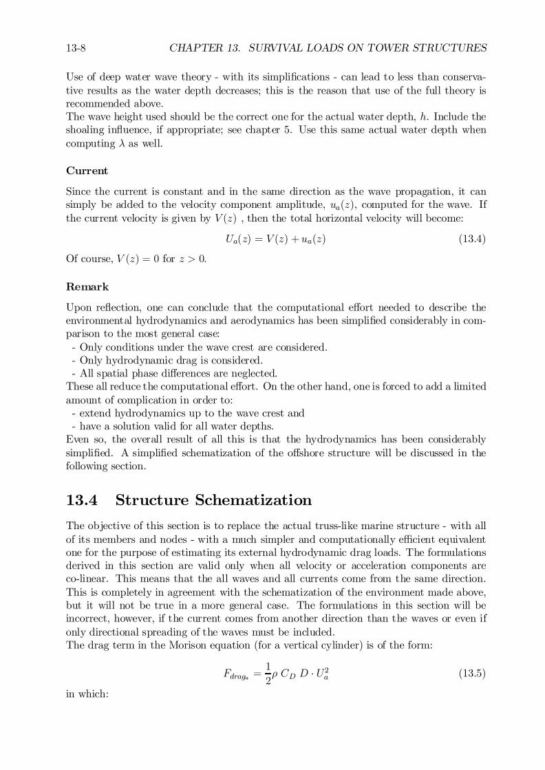
13-8 CHAPTER 13. SURVIVAL LOADS ON TOWER STRUCTURES
Use of deep water wave theory - with its simpli…cations - can lead to less than conserva-tive results as the water depth decreases; this is the reason that use of the full theory isrecommended above.The wave height used should be the correct one for the actual water depth, h. Include theshoaling in‡uence, if appropriate; see chapter 5. Use this same actual water depth whencomputing ¸ as well.
Current
Since the current is constant and in the same direction as the wave propagation, it cansimply be added to the velocity component amplitude, ua(z), computed for the wave. Ifthe current velocity is given by V (z) , then the total horizontal velocity will become:
Ua(z) = V (z) + ua(z) (13.4)
Of course, V (z) = 0 for z > 0:
Remark
Upon re‡ection, one can conclude that the computational e¤ort needed to describe theenvironmental hydrodynamics and aerodynamics has been simpli…ed considerably in com-parison to the most general case:- Only conditions under the wave crest are considered.- Only hydrodynamic drag is considered.- All spatial phase di¤erences are neglected.
These all reduce the computational e¤ort. On the other hand, one is forced to add a limitedamount of complication in order to:- extend hydrodynamics up to the wave crest and- have a solution valid for all water depths.
Even so, the overall result of all this is that the hydrodynamics has been considerablysimpli…ed. A simpli…ed schematization of the o¤shore structure will be discussed in thefollowing section.
13.4 Structure Schematization
The objective of this section is to replace the actual truss-like marine structure - with allof its members and nodes - with a much simpler and computationally e¢cient equivalentone for the purpose of estimating its external hydrodynamic drag loads. The formulationsderived in this section are valid only when all velocity or acceleration components areco-linear. This means that the all waves and all currents come from the same direction.This is completely in agreement with the schematization of the environment made above,but it will not be true in a more general case. The formulations in this section will beincorrect, however, if the current comes from another direction than the waves or even ifonly directional spreading of the waves must be included.The drag term in the Morison equation (for a vertical cylinder) is of the form:
Fdraga =1
2½ CD D ¢ U2a (13.5)
in which:

13.4. STRUCTURE SCHEMATIZATION 13-9
Fdraga = drag force amplitude per unit length of vertical cylinder (N/m)CD = drag coe¢cient, to be discussed later (-)D = cylinder diameter (m)Ua = horizontal velocity amplitude at the chosen elevation (m/s)
Since Ua will be positive in this case, Ua ¢ jUaj has been replaced by U2a .
Consider now a horizontal ’slice’ of the entire structure having a unit height; see …gure 13.1.What happens as one sums the drag forces across all the members found at that level?12½; CD; and Ua in equation 13.5 remain constant. The remaining quantity, D times a unit
height, is simply an area. Since attention focuses on the horizontal forces on the structure,this is an area projected on to a vertical plane, perpendicular to the ’slicing’ planes; it isthe area one would be able to measure on a side view photograph of the structure (if nomembers were hidden behind others in that photo!). The ’photo’ should be made lookingin the direction of wave propagation, of course.Continuing for now with a ’horizontal slice’ (of unit height) of the structure at a givenelevation, then the equivalent diameter, De; which must be used in the Morison equationdrag term (in order to get the total drag force) is simply that total area (as seen on theprojection or photo) divided by the unit height.Upon re‡ection, one will discover that at each elevation, z; one …nds the following contri-butions to De:
² Leg chords (nearly vertical) each contribute their actual diameter,D:
² Horizontal braces (if present at the chosen elevation) at an angle µ relative to theplane of water motion contribute:
De = L sin µ (13.6)
in which:
L = brace length (to the centerline of its nodes) (m)µ = brace azimuth relative to the water motion plane (rad)
but only over the limited height, D:
² Sloping braces in the plane of the picture contribute:
De =D ¢ LHB
=D
sin®=D csc® (13.7)
in which:
HB = height of the bracing bay (m); see …g. 13.1® = slope of brace relative to the horizontal (rad)
² Sloping braces in a vertical plane perpendicular to the plane of the picture (in theplane of the water motion) contribute D:
² Sloping members with other spatial orientations - think of sloping braces when wavesapproach a tower in a diagonal direction - require a bit more geometry and book-keeping. Letting:
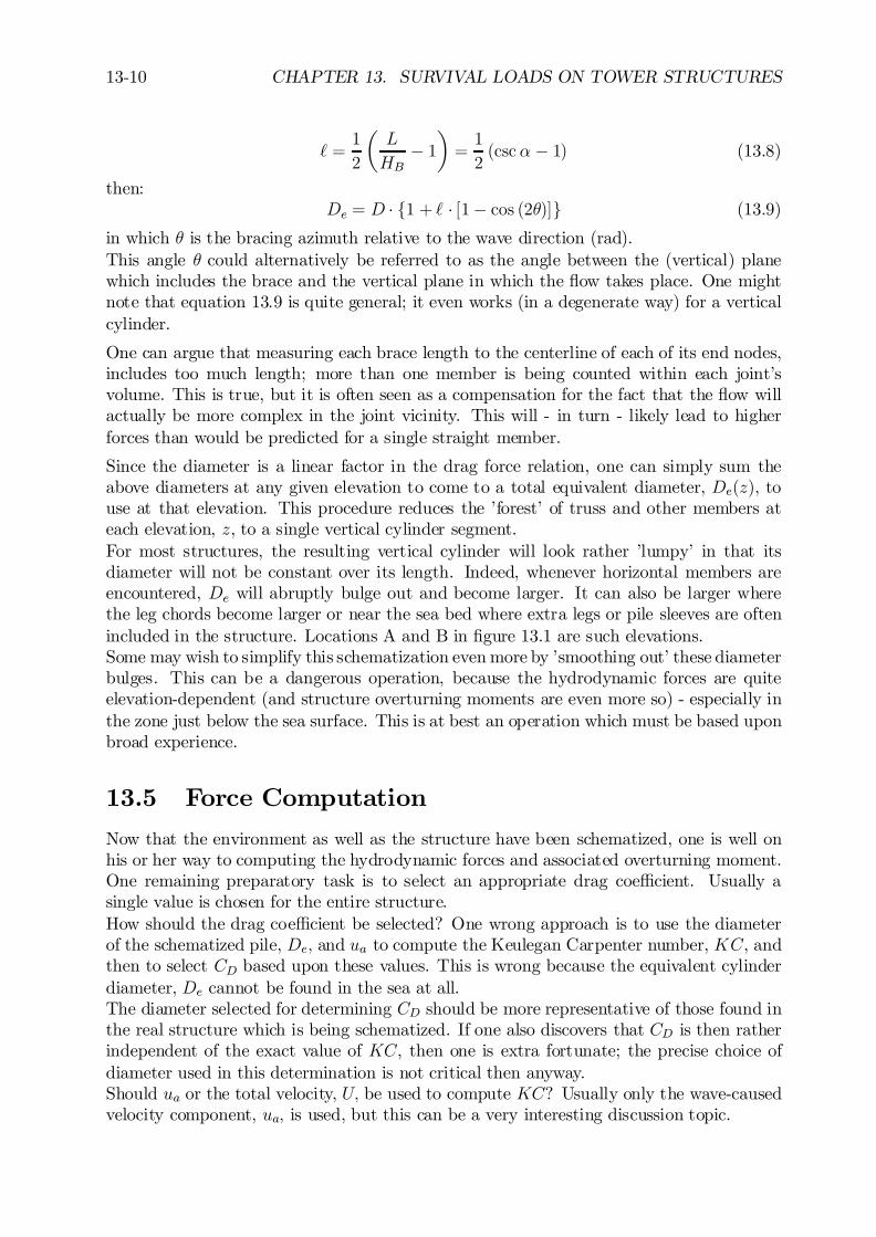
13-10 CHAPTER 13. SURVIVAL LOADS ON TOWER STRUCTURES
` =1
2
µL
HB¡ 1
¶=1
2(csc ® ¡ 1) (13.8)
then:De = D ¢ f1 + ` ¢ [1¡ cos (2µ)]g (13.9)
in which µ is the bracing azimuth relative to the wave direction (rad).This angle µ could alternatively be referred to as the angle between the (vertical) planewhich includes the brace and the vertical plane in which the ‡ow takes place. One mightnote that equation 13.9 is quite general; it even works (in a degenerate way) for a verticalcylinder.
One can argue that measuring each brace length to the centerline of each of its end nodes,includes too much length; more than one member is being counted within each joint’svolume. This is true, but it is often seen as a compensation for the fact that the ‡ow willactually be more complex in the joint vicinity. This will - in turn - likely lead to higherforces than would be predicted for a single straight member.
Since the diameter is a linear factor in the drag force relation, one can simply sum theabove diameters at any given elevation to come to a total equivalent diameter, De(z), touse at that elevation. This procedure reduces the ’forest’ of truss and other members ateach elevation, z, to a single vertical cylinder segment.For most structures, the resulting vertical cylinder will look rather ’lumpy’ in that itsdiameter will not be constant over its length. Indeed, whenever horizontal members areencountered, De will abruptly bulge out and become larger. It can also be larger wherethe leg chords become larger or near the sea bed where extra legs or pile sleeves are oftenincluded in the structure. Locations A and B in …gure 13.1 are such elevations.Some may wish to simplify this schematization even more by ’smoothing out’ these diameterbulges. This can be a dangerous operation, because the hydrodynamic forces are quiteelevation-dependent (and structure overturning moments are even more so) - especially inthe zone just below the sea surface. This is at best an operation which must be based uponbroad experience.
13.5 Force Computation
Now that the environment as well as the structure have been schematized, one is well onhis or her way to computing the hydrodynamic forces and associated overturning moment.One remaining preparatory task is to select an appropriate drag coe¢cient. Usually asingle value is chosen for the entire structure.How should the drag coe¢cient be selected? One wrong approach is to use the diameterof the schematized pile, De; and ua to compute the Keulegan Carpenter number, KC, andthen to select CD based upon these values. This is wrong because the equivalent cylinderdiameter, De cannot be found in the sea at all.The diameter selected for determining CD should be more representative of those found inthe real structure which is being schematized. If one also discovers that CD is then ratherindependent of the exact value of KC, then one is extra fortunate; the precise choice ofdiameter used in this determination is not critical then anyway.Should ua or the total velocity, U; be used to compute KC? Usually only the wave-causedvelocity component, ua; is used, but this can be a very interesting discussion topic.
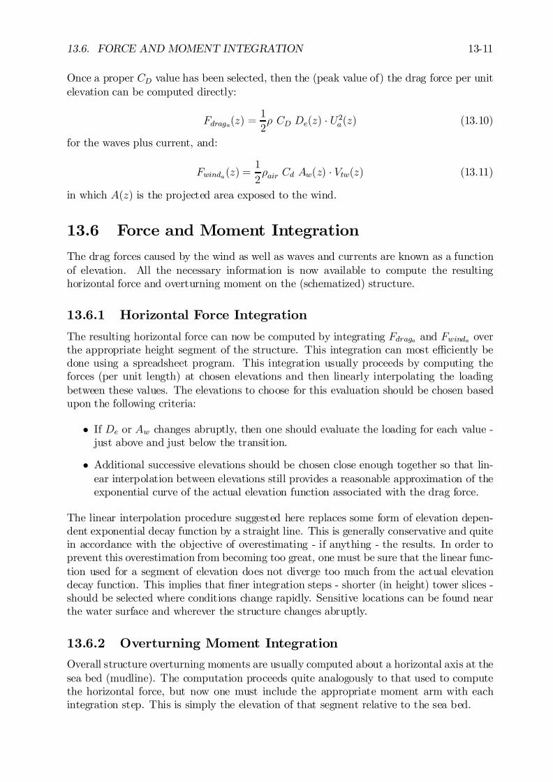
13.6. FORCE AND MOMENT INTEGRATION 13-11
Once a proper CD value has been selected, then the (peak value of) the drag force per unitelevation can be computed directly:
Fdraga(z) =1
2½ CD De(z) ¢ U2a(z) (13.10)
for the waves plus current, and:
Fwinda(z) =1
2½air Cd Aw(z) ¢ Vtw(z) (13.11)
in which A(z) is the projected area exposed to the wind.
13.6 Force and Moment Integration
The drag forces caused by the wind as well as waves and currents are known as a functionof elevation. All the necessary information is now available to compute the resultinghorizontal force and overturning moment on the (schematized) structure.
13.6.1 Horizontal Force Integration
The resulting horizontal force can now be computed by integrating Fdraga and Fwinda overthe appropriate height segment of the structure. This integration can most e¢ciently bedone using a spreadsheet program. This integration usually proceeds by computing theforces (per unit length) at chosen elevations and then linearly interpolating the loadingbetween these values. The elevations to choose for this evaluation should be chosen basedupon the following criteria:
² If De or Aw changes abruptly, then one should evaluate the loading for each value -just above and just below the transition.
² Additional successive elevations should be chosen close enough together so that lin-ear interpolation between elevations still provides a reasonable approximation of theexponential curve of the actual elevation function associated with the drag force.
The linear interpolation procedure suggested here replaces some form of elevation depen-dent exponential decay function by a straight line. This is generally conservative and quitein accordance with the objective of overestimating - if anything - the results. In order toprevent this overestimation from becoming too great, one must be sure that the linear func-tion used for a segment of elevation does not diverge too much from the actual elevationdecay function. This implies that …ner integration steps - shorter (in height) tower slices -should be selected where conditions change rapidly. Sensitive locations can be found nearthe water surface and wherever the structure changes abruptly.
13.6.2 Overturning Moment Integration
Overall structure overturning moments are usually computed about a horizontal axis at thesea bed (mudline). The computation proceeds quite analogously to that used to computethe horizontal force, but now one must include the appropriate moment arm with eachintegration step. This is simply the elevation of that segment relative to the sea bed.
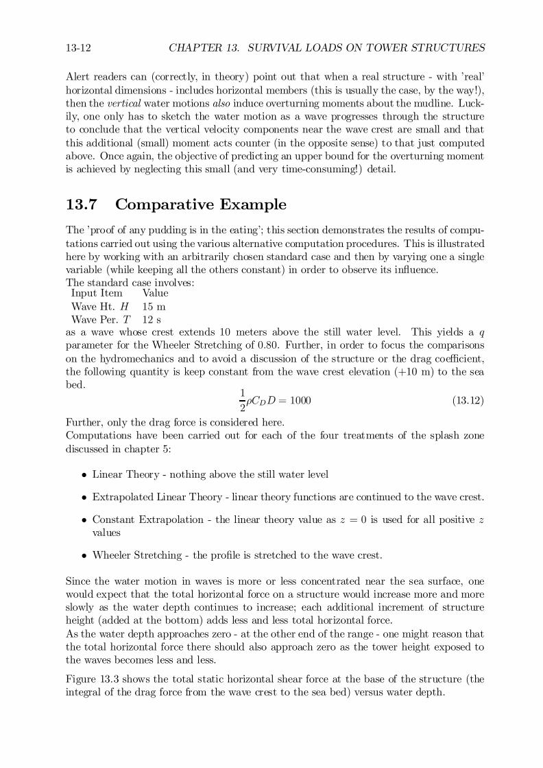
13-12 CHAPTER 13. SURVIVAL LOADS ON TOWER STRUCTURES
Alert readers can (correctly, in theory) point out that when a real structure - with ’real’horizontal dimensions - includes horizontal members (this is usually the case, by the way!),then the vertical water motions also induce overturning moments about the mudline. Luck-ily, one only has to sketch the water motion as a wave progresses through the structureto conclude that the vertical velocity components near the wave crest are small and thatthis additional (small) moment acts counter (in the opposite sense) to that just computedabove. Once again, the objective of predicting an upper bound for the overturning momentis achieved by neglecting this small (and very time-consuming!) detail.
13.7 Comparative Example
The ’proof of any pudding is in the eating’; this section demonstrates the results of compu-tations carried out using the various alternative computation procedures. This is illustratedhere by working with an arbitrarily chosen standard case and then by varying one a singlevariable (while keeping all the others constant) in order to observe its in‡uence.The standard case involves:Input Item ValueWave Ht. H 15 mWave Per. T 12 s
as a wave whose crest extends 10 meters above the still water level. This yields a qparameter for the Wheeler Stretching of 0:80. Further, in order to focus the comparisonson the hydromechanics and to avoid a discussion of the structure or the drag coe¢cient,the following quantity is keep constant from the wave crest elevation (+10 m) to the seabed.
1
2½CDD = 1000 (13.12)
Further, only the drag force is considered here.Computations have been carried out for each of the four treatments of the splash zonediscussed in chapter 5:
² Linear Theory - nothing above the still water level
² Extrapolated Linear Theory - linear theory functions are continued to the wave crest.
² Constant Extrapolation - the linear theory value as z = 0 is used for all positive zvalues
² Wheeler Stretching - the pro…le is stretched to the wave crest.
Since the water motion in waves is more or less concentrated near the sea surface, onewould expect that the total horizontal force on a structure would increase more and moreslowly as the water depth continues to increase; each additional increment of structureheight (added at the bottom) adds less and less total horizontal force.As the water depth approaches zero - at the other end of the range - one might reason thatthe total horizontal force there should also approach zero as the tower height exposed tothe waves becomes less and less.
Figure 13.3 shows the total static horizontal shear force at the base of the structure (theintegral of the drag force from the wave crest to the sea bed) versus water depth.
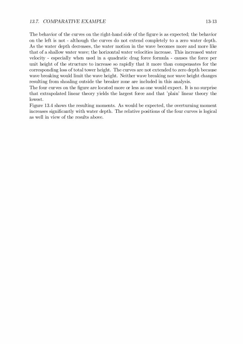
13.7. COMPARATIVE EXAMPLE 13-13
The behavior of the curves on the right-hand side of the …gure is as expected; the behavioron the left is not - although the curves do not extend completely to a zero water depth.As the water depth decreases, the water motion in the wave becomes more and more likethat of a shallow water wave; the horizontal water velocities increase. This increased watervelocity - especially when used in a quadratic drag force formula - causes the force perunit height of the structure to increase so rapidly that it more than compensates for thecorresponding loss of total tower height. The curves are not extended to zero depth becausewave breaking would limit the wave height. Neither wave breaking nor wave height changesresulting from shoaling outside the breaker zone are included in this analysis.The four curves on the …gure are located more or less as one would expect. It is no surprisethat extrapolated linear theory yields the largest force and that ’plain’ linear theory thelowest.Figure 13.4 shows the resulting moments. As would be expected, the overturning momentincreases signi…cantly with water depth. The relative positions of the four curves is logicalas well in view of the results above.
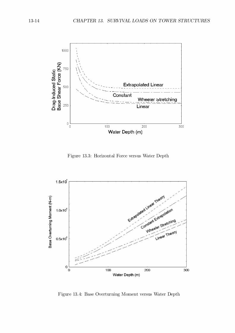
13-14 CHAPTER 13. SURVIVAL LOADS ON TOWER STRUCTURES
Figure 13.3: Horizontal Force versus Water Depth
Figure 13.4: Base Overturning Moment versus Water Depth
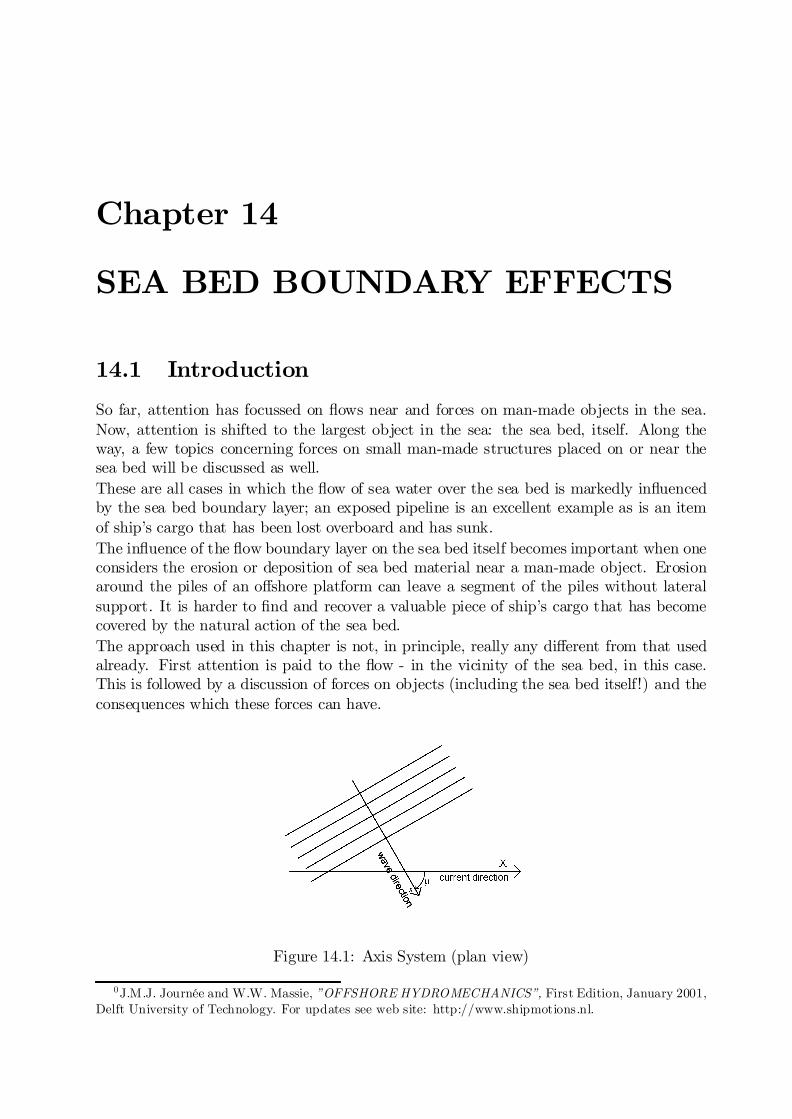
Chapter 14
SEA BED BOUNDARY EFFECTS
14.1 Introduction
So far, attention has focussed on ‡ows near and forces on man-made objects in the sea.Now, attention is shifted to the largest object in the sea: the sea bed, itself. Along theway, a few topics concerning forces on small man-made structures placed on or near thesea bed will be discussed as well.These are all cases in which the ‡ow of sea water over the sea bed is markedly in‡uencedby the sea bed boundary layer; an exposed pipeline is an excellent example as is an itemof ship’s cargo that has been lost overboard and has sunk.The in‡uence of the ‡ow boundary layer on the sea bed itself becomes important when oneconsiders the erosion or deposition of sea bed material near a man-made object. Erosionaround the piles of an o¤shore platform can leave a segment of the piles without lateralsupport. It is harder to …nd and recover a valuable piece of ship’s cargo that has becomecovered by the natural action of the sea bed.The approach used in this chapter is not, in principle, really any di¤erent from that usedalready. First attention is paid to the ‡ow - in the vicinity of the sea bed, in this case.This is followed by a discussion of forces on objects (including the sea bed itself!) and theconsequences which these forces can have.
Figure 14.1: Axis System (plan view)
0J.M.J. Journée and W.W. Massie, ”OFFSHORE HYDROMECHANICS”, First Edition, January 2001,Delft University of Technology. For updates see web site: http://www.shipmotions.nl.
14-2 CHAPTER 14. SEA BED BOUNDARY EFFECTS
The axis system shown in …gure 5.2 in chapter 5 and here in …gure 14.1 remains consistentwith that used in o¤shore engineering:- A current (if present) will ‡ow in the +X direction.- The waves propagate in the +x direction.- The positive wave direction (+x) makes an angle ¹ with the X -axis.-The +z-axis is upward from the still water level.
Note that this last convention, especially, can be in contrast to that used by coastal engi-neers (who often place the vertical coordinate origin at the sea bed). Their approach leadsto numerical computational di¢culties in deeper water.The notation for some variables used in this chapter may not agree with that often usedby coastal engineers; these changes have been made to make the notation within this bookmore consistent.
14.2 Boundary Layer under Currents and Waves
One should remember the following facts about boundary layers from basic ‡uid mechanicscourses or the earlier chapters of this book:- They result from a velocity di¤erence between the ambient ‡ow and an object.- They need time - or equivalently distance - to develop.- Surface roughness plays an important role in their development.
The second of these items is more obvious if one remembers that distance is an integrationof velocity with respect to time.What currents are important for this analysis? Tidal currents are driven by the gravita-tional attraction of the sun and the moon. These attraction forces act essentially uniformlyover the entire depth of the sea, irrespective of the water depth at the given location. (Thisis in sharp contrast to the situation with large scale oceanographic currents - which are gen-erally less than a kilometer deep - and the water motion caused by wind waves - which areeven more ’surface-bound’.) Since the tidal current driving force is uniformly distributedover the depth, one would expect that this current would also be uniformly distributed,too. This is not the case, however - at least not in the vicinity of the sea bed. Here, thecurrent is in‡uenced by a friction force resulting from the water motion over the sea bed.The Prandtl-Von Kármán logarithmic velocity distribution shown in …gure 14.2 results inthis case. Such a velocity distribution has its maximum at the sea surface and the velocityreduces very slowly at …rst, but more and more rapidly as one gets nearer - in the pro…le- to the sea bed. The exact shape of the pro…le depends upon the bed roughness.Since the logarithm of small numbers is negative, the logarithmic velocity distributionyields - strictly speaking - negative velocities in the immediate vicinity of the sea bed;this is obviously unrealistic. This shortcoming is ’patched’ by using a linear (straight line)velocity pro…le in the area nearest to the sea bed. This line has a velocity of zero at thesea bed, and is tangent to the curve of the logarithmic velocity pro…le. The velocity atthis elevation of tangency is often referred to as Vt. Obviously, this linear velocity pro…lehas a constant slope, dV
dz; if the elevation of the tangency, zt, is known and …xed, then dV
dzis simply proportional to Vt.The sea bed roughness (a length), which determines the details of the velocity pro…le canbe de…ned in either of two ways:
² If the sea bed is essentially ‡at, the roughness is de…ned in terms of the grain size ofthe sea bed material.
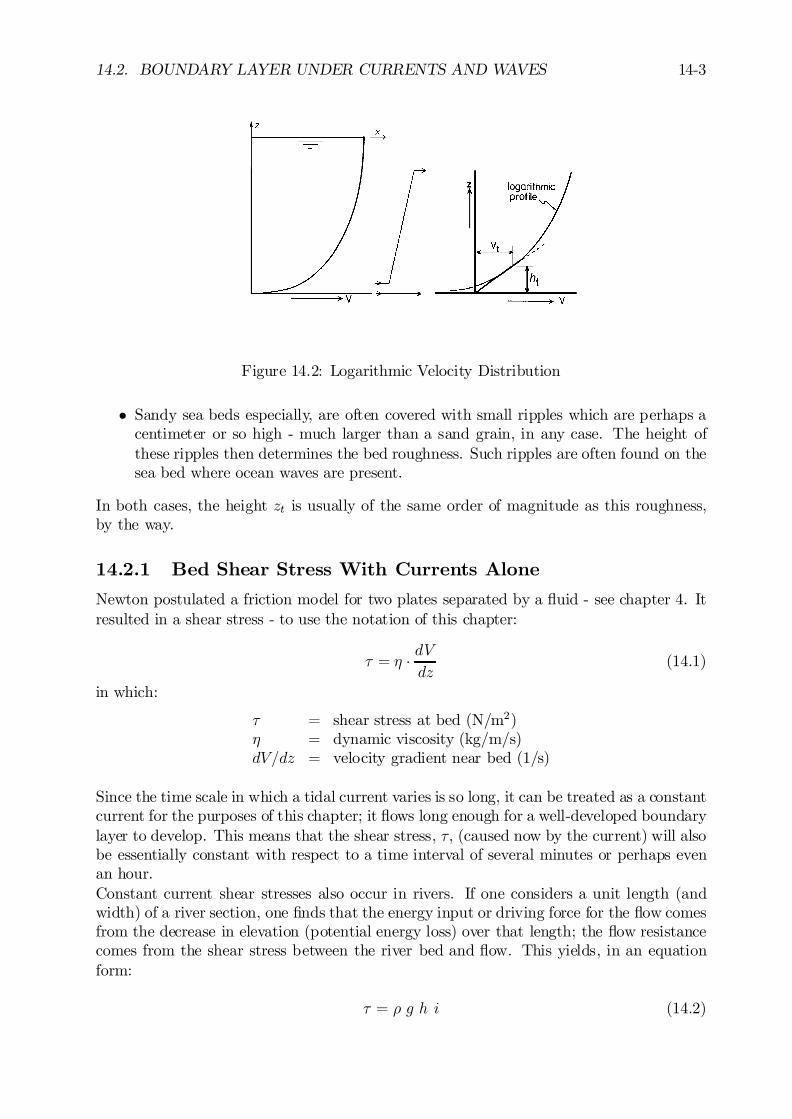
14.2. BOUNDARY LAYER UNDER CURRENTS AND WAVES 14-3
Figure 14.2: Logarithmic Velocity Distribution
² Sandy sea beds especially, are often covered with small ripples which are perhaps acentimeter or so high - much larger than a sand grain, in any case. The height ofthese ripples then determines the bed roughness. Such ripples are often found on thesea bed where ocean waves are present.
In both cases, the height zt is usually of the same order of magnitude as this roughness,by the way.
14.2.1 Bed Shear Stress With Currents Alone
Newton postulated a friction model for two plates separated by a ‡uid - see chapter 4. Itresulted in a shear stress - to use the notation of this chapter:
¿ = ´ ¢ dVdz
(14.1)
in which:
¿ = shear stress at bed (N/m2)´ = dynamic viscosity (kg/m/s)dV=dz = velocity gradient near bed (1/s)
Since the time scale in which a tidal current varies is so long, it can be treated as a constantcurrent for the purposes of this chapter; it ‡ows long enough for a well-developed boundarylayer to develop. This means that the shear stress, ¿, (caused now by the current) will alsobe essentially constant with respect to a time interval of several minutes or perhaps evenan hour.Constant current shear stresses also occur in rivers. If one considers a unit length (andwidth) of a river section, one …nds that the energy input or driving force for the ‡ow comesfrom the decrease in elevation (potential energy loss) over that length; the ‡ow resistancecomes from the shear stress between the river bed and ‡ow. This yields, in an equationform:
¿ = ½ g h i (14.2)

14-4 CHAPTER 14. SEA BED BOUNDARY EFFECTS
in which:
¿ = bed shear stress (N/m2)½ = mass density of water (kg/m3)g = acceleration of gravity (m/s2)h = water depth (m)i = river surface slope dz=dx in the direction of ‡ow (-)
In the eighteenth century, the French hydraulic engineer, Antoine Chézy, developed anempirical relationship for the depth-averaged velocity in a river. The earliest know recordof its publication is 1775. It is quite certainly the …rst uniform ‡ow formula for openchannels; it is still used today. It is a formula:
V = Cph i (14.3)
in which C is an empirical coe¢cient which is not dimensionless; it has units of m1=2=s. Italso has an inverse relation to the bed roughness: the rougher the bed, the lower the valueof C.It can be convenient to combine equations 14.2 and 14.3. Since there is essentially noconstant water surface slope o¤shore, one simply eliminates the slope term, i, from theabove two equations. This yields:
¿ = ½ gV 2
C2(14.4)
Notice that the water depth falls out of this equation, too, but C must still be estimated.This can be done for a constant current (at least) using:
C = 18 log12 h
r(14.5)
in which:C = Chézy Coe¢cient (m
12/s)
h = water depth (m)r = bed roughness (m)
All of this brings up an interesting question: Since Vt - the current velocity at the elevationof the point of tangency - is directly proportional to the average velocity, V , how doesone explain that Newton’s approach relates ¿ to V , while at the same time, Chézy (see[Herschel, 1897]) relates ¿ to V 2? One of these must be wrong, or there may be anotherexplanation.One is not sure that C (or even ´ for that matter) remains constant for a wide variety of‡ow conditions. Indeed, every river engineer knows that C is not constant. In practice,there is generally more faith in Chézy than in Newton in this case, however, so that ¿ isusually associated with a higher power of V or dV=dz:The shear stress, ¿ , discussed so far has been the shear stress which the sea bed exertson the ‡ow. Newton’s Third Law of motion indicates, however, that this is also the shearstress which the ‡ow exerts on the sea bed.Before proceeding with this development, the discussion backtracks to discuss the boundarylayer and shear stress under waves.
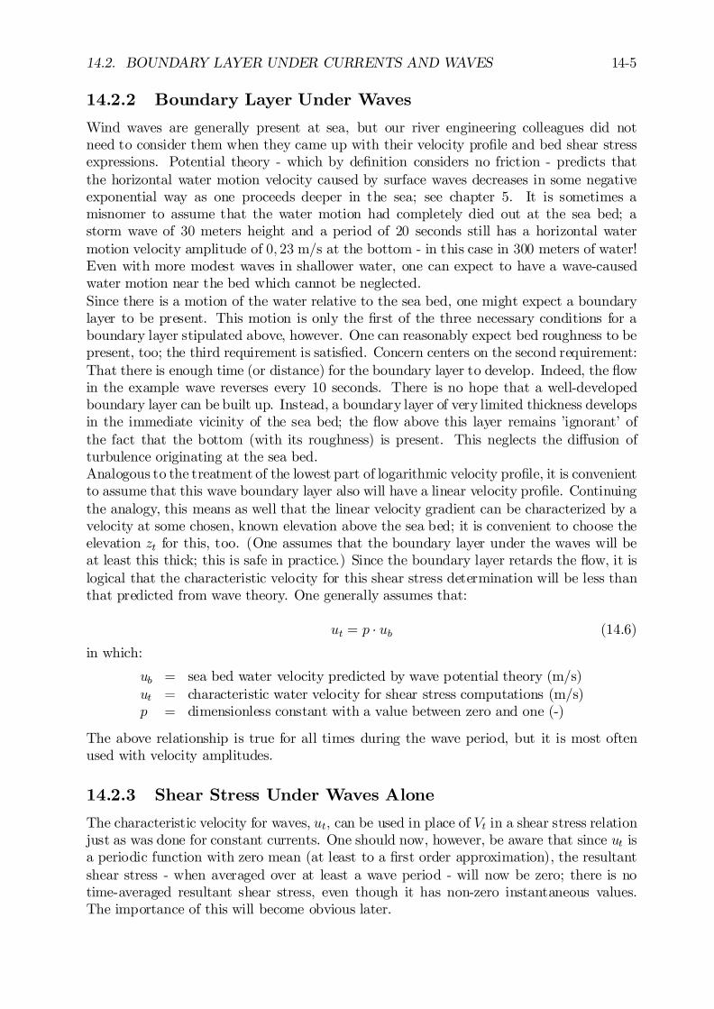
14.2. BOUNDARY LAYER UNDER CURRENTS AND WAVES 14-5
14.2.2 Boundary Layer Under Waves
Wind waves are generally present at sea, but our river engineering colleagues did notneed to consider them when they came up with their velocity pro…le and bed shear stressexpressions. Potential theory - which by de…nition considers no friction - predicts thatthe horizontal water motion velocity caused by surface waves decreases in some negativeexponential way as one proceeds deeper in the sea; see chapter 5. It is sometimes amisnomer to assume that the water motion had completely died out at the sea bed; astorm wave of 30 meters height and a period of 20 seconds still has a horizontal watermotion velocity amplitude of 0; 23 m/s at the bottom - in this case in 300 meters of water!Even with more modest waves in shallower water, one can expect to have a wave-causedwater motion near the bed which cannot be neglected.Since there is a motion of the water relative to the sea bed, one might expect a boundarylayer to be present. This motion is only the …rst of the three necessary conditions for aboundary layer stipulated above, however. One can reasonably expect bed roughness to bepresent, too; the third requirement is satis…ed. Concern centers on the second requirement:That there is enough time (or distance) for the boundary layer to develop. Indeed, the ‡owin the example wave reverses every 10 seconds. There is no hope that a well-developedboundary layer can be built up. Instead, a boundary layer of very limited thickness developsin the immediate vicinity of the sea bed; the ‡ow above this layer remains ’ignorant’ ofthe fact that the bottom (with its roughness) is present. This neglects the di¤usion ofturbulence originating at the sea bed.Analogous to the treatment of the lowest part of logarithmic velocity pro…le, it is convenientto assume that this wave boundary layer also will have a linear velocity pro…le. Continuingthe analogy, this means as well that the linear velocity gradient can be characterized by avelocity at some chosen, known elevation above the sea bed; it is convenient to choose theelevation zt for this, too. (One assumes that the boundary layer under the waves will beat least this thick; this is safe in practice.) Since the boundary layer retards the ‡ow, it islogical that the characteristic velocity for this shear stress determination will be less thanthat predicted from wave theory. One generally assumes that:
ut = p ¢ ub (14.6)
in which:
ub = sea bed water velocity predicted by wave potential theory (m/s)ut = characteristic water velocity for shear stress computations (m/s)p = dimensionless constant with a value between zero and one (-)
The above relationship is true for all times during the wave period, but it is most oftenused with velocity amplitudes.
14.2.3 Shear Stress Under Waves Alone
The characteristic velocity for waves, ut; can be used in place of Vt in a shear stress relationjust as was done for constant currents. One should now, however, be aware that since ut isa periodic function with zero mean (at least to a …rst order approximation), the resultantshear stress - when averaged over at least a wave period - will now be zero; there is notime-averaged resultant shear stress, even though it has non-zero instantaneous values.The importance of this will become obvious later.
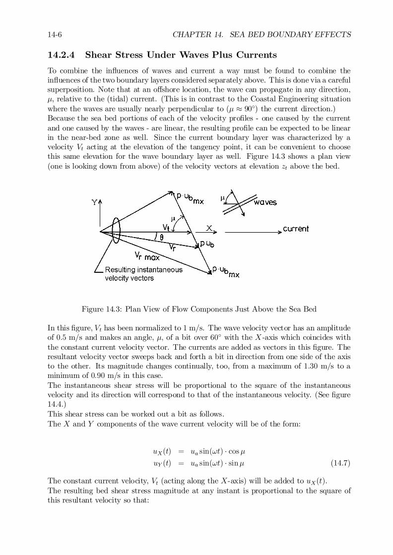
14-6 CHAPTER 14. SEA BED BOUNDARY EFFECTS
14.2.4 Shear Stress Under Waves Plus Currents
To combine the in‡uences of waves and current a way must be found to combine thein‡uences of the two boundary layers considered separately above. This is done via a carefulsuperposition. Note that at an o¤shore location, the wave can propagate in any direction,¹, relative to the (tidal) current. (This is in contrast to the Coastal Engineering situationwhere the waves are usually nearly perpendicular to (¹ ¼ 90±) the current direction.)Because the sea bed portions of each of the velocity pro…les - one caused by the currentand one caused by the waves - are linear, the resulting pro…le can be expected to be linearin the near-bed zone as well. Since the current boundary layer was characterized by avelocity Vt acting at the elevation of the tangency point, it can be convenient to choosethis same elevation for the wave boundary layer as well. Figure 14.3 shows a plan view(one is looking down from above) of the velocity vectors at elevation zt above the bed.
Figure 14.3: Plan View of Flow Components Just Above the Sea Bed
In this …gure, Vt has been normalized to 1 m/s. The wave velocity vector has an amplitudeof 0:5 m/s and makes an angle, ¹; of a bit over 60± with the X -axis which coincides withthe constant current velocity vector. The currents are added as vectors in this …gure. Theresultant velocity vector sweeps back and forth a bit in direction from one side of the axisto the other. Its magnitude changes continually, too, from a maximum of 1:30 m/s to aminimum of 0:90 m/s in this case.The instantaneous shear stress will be proportional to the square of the instantaneousvelocity and its direction will correspond to that of the instantaneous velocity. (See …gure14.4.)This shear stress can be worked out a bit as follows.The X and Y components of the wave current velocity will be of the form:
uX(t) = ua sin(!t) ¢ cos¹uY (t) = ua sin(!t) ¢ sin¹ (14.7)
The constant current velocity, Vt (acting along the X-axis) will be added to uX(t).The resulting bed shear stress magnitude at any instant is proportional to the square ofthis resultant velocity so that:
14.2. BOUNDARY LAYER UNDER CURRENTS AND WAVES 14-7
Figure 14.4: Instantaneous Shear Stresses Under Waves Plus Currents
jV 2r j = (Vt + uX(t))2 + (uY (t))
2
=¡V 2t + 2 Vt ¢ ua sin(!t) ¢ cos¹+ u2a sin2(!t) ¢ cos2 ¹
¢(14.8)
+u2a sin2(!t) ¢ sin2 ¹ (14.9)
The instantaneous magnitude of the resulting shear stress, ¿, is directly proportional tothis.
Time Averaged Shear Stress Magnitude
The magnitude of ¿ can be averaged over a wave period as well so that:
¿ cw = j¿ j ® V 2t + 0+1
2u2a ¢ cos2 ¹+ 1
2u2a ¢ sin2 ¹ (14.10)
Noting that: cos2 ¹+ sin2 ¹ = 1, one comes to the …nal conclusion that:
¿ cw = j¿ j ® V 2t +1
2u2a (14.11)
which happens to be completely independent of ¹ ! In these equations (with all velocitiesat height z = zt):
¿ cw = time averaged bed shear stress (N/m2)Vt = current velocity (m/s)ua = amplitude of the wave motion (includes the factor, p) (m/s)¹ = angle between the wave propagation and current directions (rad)
This average magnitude of the bed shear stress (independent of its direction) will be foundlater to be important for the determination of sediment transport. Equation 14.11 makesvery clear that both the current and the waves contribute to the bed shear stress; waves,if present, generally increase the average bed shear stress - in spite of the fact that theaverage shear stress under the waves alone is identically zero as indicated earlier in thischapter.
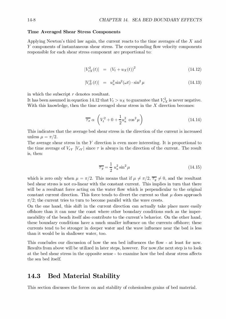
14-8 CHAPTER 14. SEA BED BOUNDARY EFFECTS
Time Averaged Shear Stress Components
Applying Newton’s third law again, the current reacts to the time averages of the X andY components of instantaneous shear stress. The corresponding ‡ow velocity componentsresponsible for each shear stress component are proportional to:
jV 2rX(t)j = (Vt + uX(t))2 (14.12)
jV 2rY (t)j = u2a sin2(!t) ¢ sin2 ¹ (14.13)
in which the subscript r denotes resultant.It has been assumed in equation 14.12 that Vt > uX to guarantee that V 2rX is never negative.With this knowledge, then the time averaged shear stress in the X direction becomes:
¿x ®
µV 2t +0 +
1
2u2a cos
2¹
¶(14.14)
This indicates that the average bed shear stress in the direction of the current is increasedunless ¹ = ¼=2.The average shear stress in the Y direction is even more interesting. It is proportional tothe time average of VrY jVrY j since ¿ is always in the direction of the current. The resultis, then:
¿ y =1
2u2a sin
2 ¹ (14.15)
which is zero only when ¹ = ¼=2. This means that if ¹ 6= ¼=2, ¿y 6= 0, and the resultantbed shear stress is not co-linear with the constant current. This implies in turn that therewill be a resultant force acting on the water ‡ow which is perpendicular to the originalconstant current direction. This force tends to divert the current so that ¹ does approach¼=2; the current tries to turn to become parallel with the wave crests.On the one hand, this shift in the current direction can actually take place more easilyo¤shore than it can near the coast where other boundary conditions such as the imper-meability of the beach itself also contribute to the current’s behavior. On the other hand,these boundary conditions have a much smaller in‡uence on the currents o¤shore; thesecurrents tend to be stronger in deeper water and the wave in‡uence near the bed is lessthan it would be in shallower water, too.
This concludes our discussion of how the sea bed in‡uences the ‡ow - at least for now.Results from above will be utilized in later steps, however. For now,the next step is to lookat the bed shear stress in the opposite sense - to examine how the bed shear stress a¤ectsthe sea bed itself.
14.3 Bed Material Stability
This section discusses the forces on and stability of cohesionless grains of bed material.
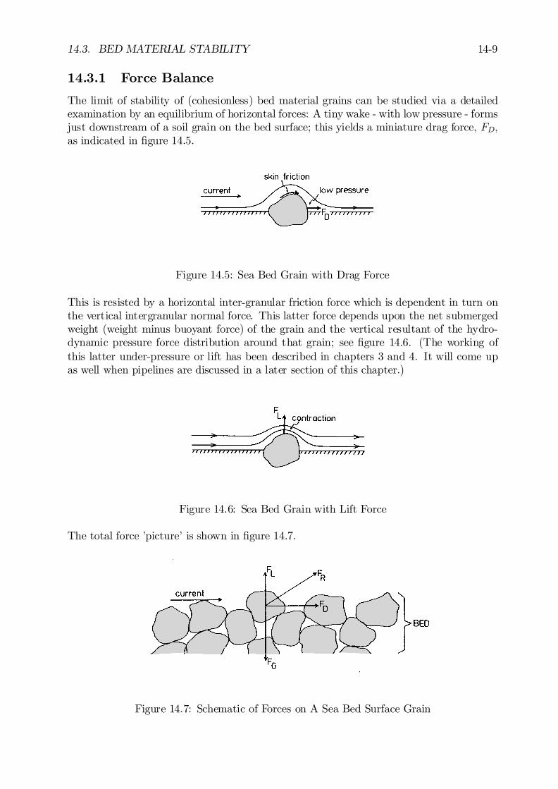
14.3. BED MATERIAL STABILITY 14-9
14.3.1 Force Balance
The limit of stability of (cohesionless) bed material grains can be studied via a detailedexamination by an equilibrium of horizontal forces: A tiny wake - with low pressure - formsjust downstream of a soil grain on the bed surface; this yields a miniature drag force, FD;as indicated in …gure 14.5.
Figure 14.5: Sea Bed Grain with Drag Force
This is resisted by a horizontal inter-granular friction force which is dependent in turn onthe vertical intergranular normal force. This latter force depends upon the net submergedweight (weight minus buoyant force) of the grain and the vertical resultant of the hydro-dynamic pressure force distribution around that grain; see …gure 14.6. (The working ofthis latter under-pressure or lift has been described in chapters 3 and 4. It will come upas well when pipelines are discussed in a later section of this chapter.)
Figure 14.6: Sea Bed Grain with Lift Force
The total force ’picture’ is shown in …gure 14.7.
Figure 14.7: Schematic of Forces on A Sea Bed Surface Grain
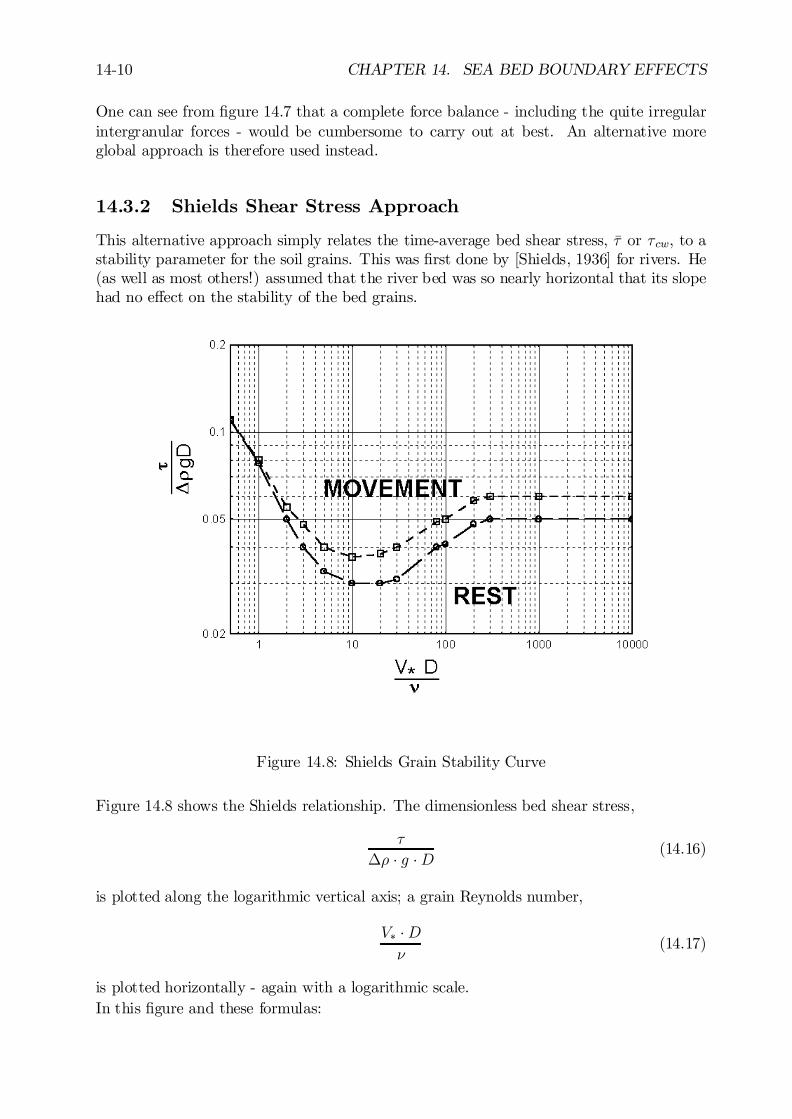
14-10 CHAPTER 14. SEA BED BOUNDARY EFFECTS
One can see from …gure 14.7 that a complete force balance - including the quite irregularintergranular forces - would be cumbersome to carry out at best. An alternative moreglobal approach is therefore used instead.
14.3.2 Shields Shear Stress Approach
This alternative approach simply relates the time-average bed shear stress, ¹¿ or ¿cw, to astability parameter for the soil grains. This was …rst done by [Shields, 1936] for rivers. He(as well as most others!) assumed that the river bed was so nearly horizontal that its slopehad no e¤ect on the stability of the bed grains.
Figure 14.8: Shields Grain Stability Curve
Figure 14.8 shows the Shields relationship. The dimensionless bed shear stress,
¿
¢½ ¢ g ¢D (14.16)
is plotted along the logarithmic vertical axis; a grain Reynolds number,
V¤ ¢Dº
(14.17)
is plotted horizontally - again with a logarithmic scale.In this …gure and these formulas:
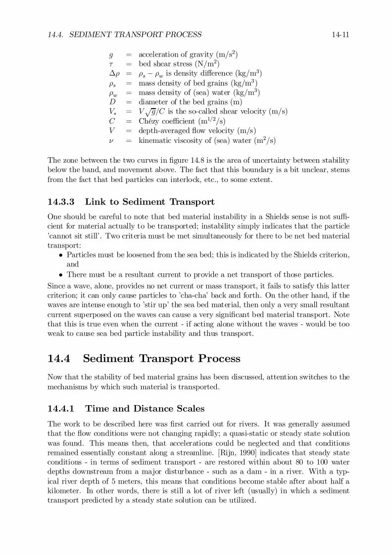
14.4. SEDIMENT TRANSPORT PROCESS 14-11
g = acceleration of gravity (m/s2)¿ = bed shear stress (N/m2)¢½ = ½s ¡ ½w is density di¤erence (kg/m3)½s = mass density of bed grains (kg/m3)½w = mass density of (sea) water (kg/m3)D = diameter of the bed grains (m)V¤ = V
pg=C is the so-called shear velocity (m/s)
C = Chézy coe¢cient (m1=2/s)V = depth-averaged ‡ow velocity (m/s)º = kinematic viscosity of (sea) water (m2/s)
The zone between the two curves in …gure 14.8 is the area of uncertainty between stabilitybelow the band, and movement above. The fact that this boundary is a bit unclear, stemsfrom the fact that bed particles can interlock, etc., to some extent.
14.3.3 Link to Sediment Transport
One should be careful to note that bed material instability in a Shields sense is not su¢-cient for material actually to be transported; instability simply indicates that the particle’cannot sit still’. Two criteria must be met simultaneously for there to be net bed materialtransport:
² Particles must be loosened from the sea bed; this is indicated by the Shields criterion,and
² There must be a resultant current to provide a net transport of those particles.
Since a wave, alone, provides no net current or mass transport, it fails to satisfy this lattercriterion; it can only cause particles to ’cha-cha’ back and forth. On the other hand, if thewaves are intense enough to ’stir up’ the sea bed material, then only a very small resultantcurrent superposed on the waves can cause a very signi…cant bed material transport. Notethat this is true even when the current - if acting alone without the waves - would be tooweak to cause sea bed particle instability and thus transport.
14.4 Sediment Transport Process
Now that the stability of bed material grains has been discussed, attention switches to themechanisms by which such material is transported.
14.4.1 Time and Distance Scales
The work to be described here was …rst carried out for rivers. It was generally assumedthat the ‡ow conditions were not changing rapidly; a quasi-static or steady state solutionwas found. This means then, that accelerations could be neglected and that conditionsremained essentially constant along a streamline. [Rijn, 1990] indicates that steady stateconditions - in terms of sediment transport - are restored within about 80 to 100 waterdepths downstream from a major disturbance - such as a dam - in a river. With a typ-ical river depth of 5 meters, this means that conditions become stable after about half akilometer. In other words, there is still a lot of river left (usually) in which a sedimenttransport predicted by a steady state solution can be utilized.
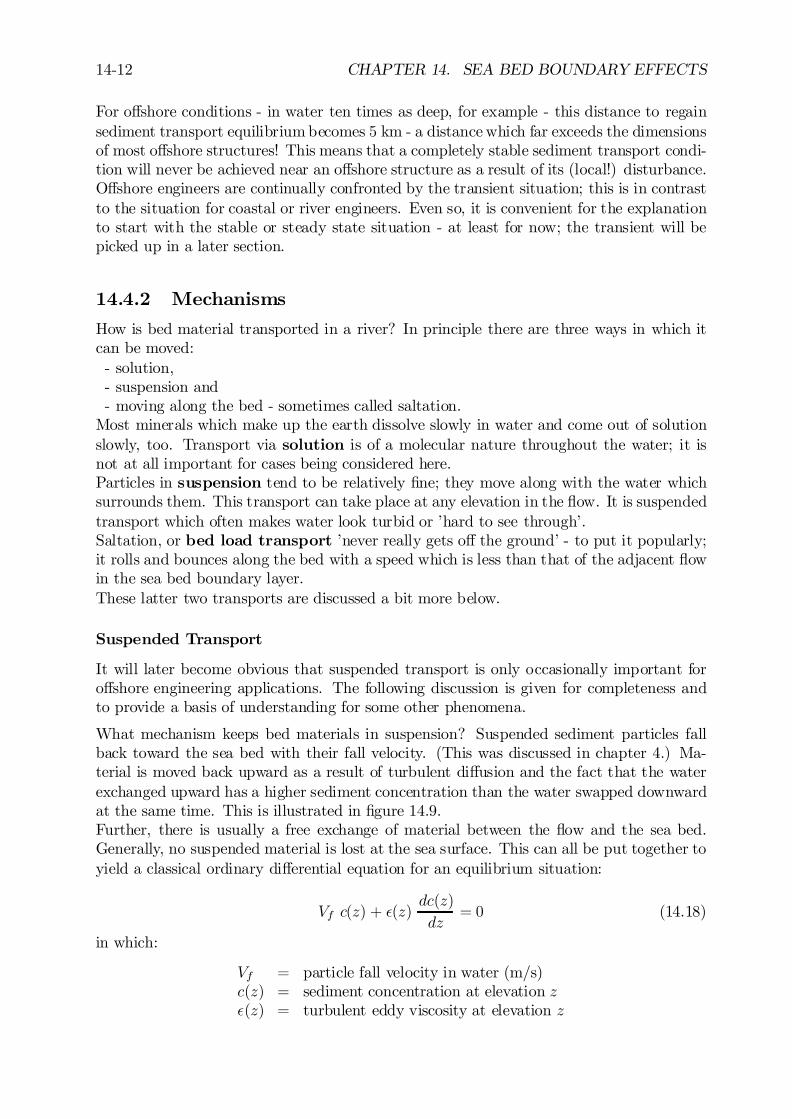
14-12 CHAPTER 14. SEA BED BOUNDARY EFFECTS
For o¤shore conditions - in water ten times as deep, for example - this distance to regainsediment transport equilibrium becomes 5 km - a distance which far exceeds the dimensionsof most o¤shore structures! This means that a completely stable sediment transport condi-tion will never be achieved near an o¤shore structure as a result of its (local!) disturbance.O¤shore engineers are continually confronted by the transient situation; this is in contrastto the situation for coastal or river engineers. Even so, it is convenient for the explanationto start with the stable or steady state situation - at least for now; the transient will bepicked up in a later section.
14.4.2 Mechanisms
How is bed material transported in a river? In principle there are three ways in which itcan be moved:- solution,- suspension and- moving along the bed - sometimes called saltation.
Most minerals which make up the earth dissolve slowly in water and come out of solutionslowly, too. Transport via solution is of a molecular nature throughout the water; it isnot at all important for cases being considered here.Particles in suspension tend to be relatively …ne; they move along with the water whichsurrounds them. This transport can take place at any elevation in the ‡ow. It is suspendedtransport which often makes water look turbid or ’hard to see through’.Saltation, or bed load transport ’never really gets o¤ the ground’ - to put it popularly;it rolls and bounces along the bed with a speed which is less than that of the adjacent ‡owin the sea bed boundary layer.These latter two transports are discussed a bit more below.
Suspended Transport
It will later become obvious that suspended transport is only occasionally important foro¤shore engineering applications. The following discussion is given for completeness andto provide a basis of understanding for some other phenomena.
What mechanism keeps bed materials in suspension? Suspended sediment particles fallback toward the sea bed with their fall velocity. (This was discussed in chapter 4.) Ma-terial is moved back upward as a result of turbulent di¤usion and the fact that the waterexchanged upward has a higher sediment concentration than the water swapped downwardat the same time. This is illustrated in …gure 14.9.Further, there is usually a free exchange of material between the ‡ow and the sea bed.Generally, no suspended material is lost at the sea surface. This can all be put together toyield a classical ordinary di¤erential equation for an equilibrium situation:
Vf c(z) + ²(z)dc(z)
dz= 0 (14.18)
in which:
Vf = particle fall velocity in water (m/s)c(z) = sediment concentration at elevation z²(z) = turbulent eddy viscosity at elevation z
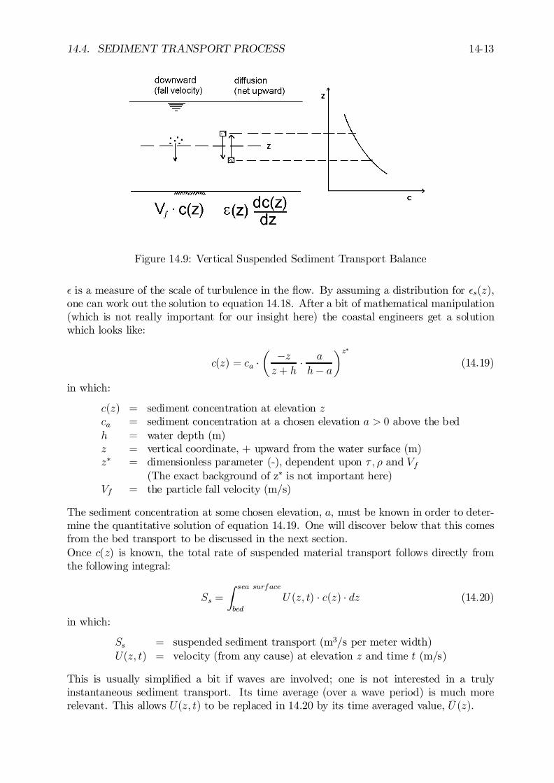
14.4. SEDIMENT TRANSPORT PROCESS 14-13
Figure 14.9: Vertical Suspended Sediment Transport Balance
² is a measure of the scale of turbulence in the ‡ow. By assuming a distribution for ²s(z),one can work out the solution to equation 14.18. After a bit of mathematical manipulation(which is not really important for our insight here) the coastal engineers get a solutionwhich looks like:
c(z) = ca ¢µ ¡zz + h
¢ a
h¡ a
¶z¤
(14.19)
in which:
c(z) = sediment concentration at elevation zca = sediment concentration at a chosen elevation a > 0 above the bedh = water depth (m)z = vertical coordinate, + upward from the water surface (m)z¤ = dimensionless parameter (-), dependent upon ¿ ; ½ and Vf
(The exact background of z¤ is not important here)Vf = the particle fall velocity (m/s)
The sediment concentration at some chosen elevation, a; must be known in order to deter-mine the quantitative solution of equation 14.19. One will discover below that this comesfrom the bed transport to be discussed in the next section.Once c(z) is known, the total rate of suspended material transport follows directly fromthe following integral:
Ss =
Z sea surface
bed
U (z; t) ¢ c(z) ¢ dz (14.20)
in which:
Ss = suspended sediment transport (m3/s per meter width)U(z; t) = velocity (from any cause) at elevation z and time t (m/s)
This is usually simpli…ed a bit if waves are involved; one is not interested in a trulyinstantaneous sediment transport. Its time average (over a wave period) is much morerelevant. This allows U(z; t) to be replaced in 14.20 by its time averaged value, ¹U (z):
14-14 CHAPTER 14. SEA BED BOUNDARY EFFECTS
Bed Load Transport
Bed load transport ’never gets o¤ the ground’; it stays near the bed in a thin layer belowthe suspended sediment transport. The same forces which determine particle stability alsogovern bed load transport. In contrast to the situation with suspended transport, the bedload moves more slowly than the water near the bed; most formulas for predicting the rateof bed load transport, Sb, express this rate directly instead of via a concentration timesa velocity as was done with suspended transport. Indeed, the water velocity is changingrapidly as a function of elevation here and the sediment concentration is hard to de…ne inthis region, too.On the other hand, a sediment concentration - at some elevation - is needed in order todetermine the actual suspended sediment concentration pro…le as explained above. It isconvenient to perform this coupling near the sea bed - more speci…cally at an elevationht above the bed - the height at which the linear near-bed velocity pro…le is tangent tothe logarithmic Prandtl-Von Kármán pro…le. It is being assumed (quite arbitrarily) thattransport above this level takes place in suspension and that only bed load transport isfound below.Hydraulic engineers have taken the very pragmatic step of converting the bed load transportinto a (form of) concentration by assuming that Sb takes place in a layer of thickness htand with a velocity equal to Vt. This equivalent ’concentration’ is then:
ca =Sbht ¢ Vt
(14.21)
Using this link, one can relate the entire steady state sediment transport, S = Sb + Ss,to one quantity: The bed transport, Sb. Attention can be concentrated on determiningthis value. Before doing so, however, the relative importance of Sb and Ss for o¤shoreapplications will be examined in this next section.
14.4.3 Relative Importance of Bed versus Suspended Load
Many comparisons can be included under this heading. River engineers are often interestedin the ratio of suspended load transport to bed load transport, Ss=Sb. This value can varywidely in rivers, by the way; it can be high (thousands) for a muddy river such as theAmazon or Mississippi, and very low (¿ 1) for a sparkling clear mountain stream tumblingover rocks.
In o¤shore engineering on the other hand, one is wise to …rst consider the relative time(or distance) scales within which Sb or Ss change. Consider what happens to each of thesequantities when - for example - the near-bed ‡ow is locally disturbed by a partially exposedsubmarine pipeline, for example. Such a pipeline will typically be no more than a meter indiameter and it may protrude 50 centimeters or so above the sea bed. At the same time,the water depth can easily be in the order of 100 meters.Using potential theory from chapter 3 to estimate the order of magnitude of the disturbancecaused by the half-buried pipe, one …nds that at a distance of at little as 1 meter abovethe sea bed (above the pipe) the velocity has only been increased by 25%. At 2 metersheight this increase is only a bit more than 6%. The conclusion must be that the pipe onlydisturbs the velocity …eld in its immediate vicinity. Consequently, the velocity gradientsand thus the local bed shear stresses and vertical di¤usion of sediment will be disturbedonly locally as well.
14.5. SEA BED CHANGES 14-15
One can expect the bed transport, Sb, to react quickly to these changes. Indeed, eachbed transport particle can stop any time it hits the bottom and this happens almostcontinuously. The bed transport can adjust or adapt itself several times within a distanceof a few meters.The material making up the suspended transport, Ss, on the other hand, does not fre-quently come in contact with the bottom; it gets little opportunity to stop. Except that‡ow in the immediate vicinity of the pipe - especially in its wake - may be a bit more tur-bulent, the rest of the (tidal current) ‡ow does not even ’notice’ that the pipe is there; themajor part of the ‡ow as well as the suspended transport it carries is essentially undisturbedby such small scale changes.
Some may argue that whenever Sb changes, Ss will change as well. Their reasoning followsfrom the link established above between suspended and bed load transports. What theyfail to realize is that this theoretical ’link’ was established for an equilibrium situationand that a change in Ss must take place via changes in its sediment concentration pro…le.The driving forces for determining that pro…le - the turbulent di¤usion and the particle fallvelocity - are not (or only very locally) changed. It is indeed because of Ss that [Rijn, 1990]concluded that a distance of 80 to 100 water depths is needed for an equilibrium sedimenttransport to be reached in a river.
The conclusion to all this is that bed load transport reacts very quickly to ‡ow changeswhich occur on a scale typical of o¤shore engineering objects, but that suspended transportdoes not. O¤shore engineers seldom have to worry about the transport of suspendedmaterial. Sb is almost always the most important transport component in an o¤shoresituation. Conversely, Ss is seldom important in an o¤shore situation!
14.5 Sea Bed Changes
14.5.1 Sediment Transport Not Su¢cient for Bed Changes
Having bed material instability (in the Shields sense) and having a resulting current totransport that material is not usually su¢cient to cause a real morphological problem(erosion or deposition). The presence of sediment transport past a point only indicatesthat the bed material grains now present at that location will (probably) be replaced byothers within a very short time; a dynamic equilibrium can exist.In order to have (or reveal) morphological changes as a result of sediment transport, onemust examine dS=dX, the change in sediment transport along a (resulting) streamline. If Sincreases as the ‡ow proceeds from point A to point B, as shown in schematic cross sectionin …gure 14.10, then the extra material transported past point B (if dS=dX is positive)can only have come from the bed segment between A and B; a positive value of dS=dXleads to erosion. Conversely, a negative value must lead to sedimentation or deposition ofmaterial in the segment between A and B.How does a time dependence a¤ect the situation? When the current changes slowly as afunction of time - such as with a tidal current - this makes no di¤erence. This variationonly introduces a dS=dt which is pretty much the same in the entire vicinity; this does not- of itself - yield either a signi…cant erosion or deposition.
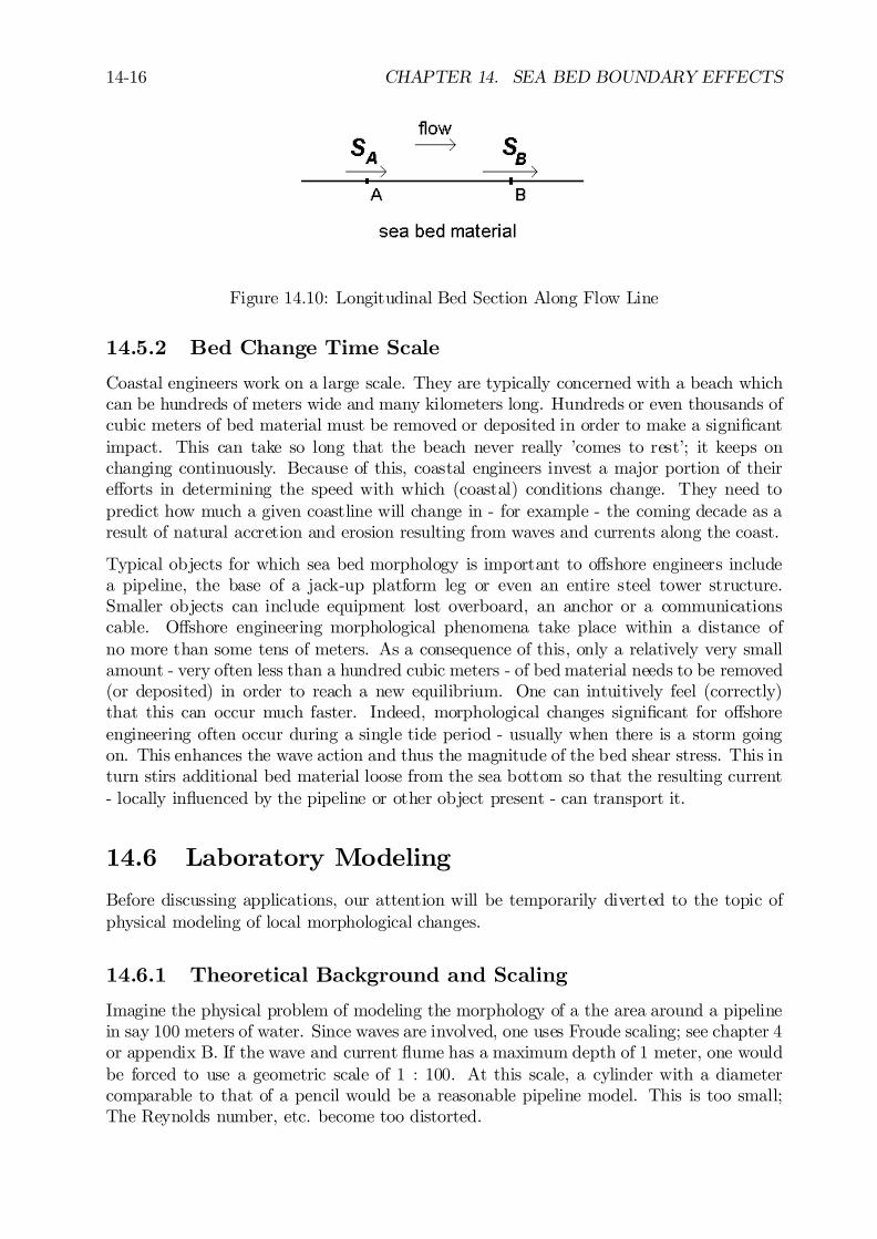
14-16 CHAPTER 14. SEA BED BOUNDARY EFFECTS
Figure 14.10: Longitudinal Bed Section Along Flow Line
14.5.2 Bed Change Time Scale
Coastal engineers work on a large scale. They are typically concerned with a beach whichcan be hundreds of meters wide and many kilometers long. Hundreds or even thousands ofcubic meters of bed material must be removed or deposited in order to make a signi…cantimpact. This can take so long that the beach never really ’comes to rest’; it keeps onchanging continuously. Because of this, coastal engineers invest a major portion of theire¤orts in determining the speed with which (coastal) conditions change. They need topredict how much a given coastline will change in - for example - the coming decade as aresult of natural accretion and erosion resulting from waves and currents along the coast.
Typical objects for which sea bed morphology is important to o¤shore engineers includea pipeline, the base of a jack-up platform leg or even an entire steel tower structure.Smaller objects can include equipment lost overboard, an anchor or a communicationscable. O¤shore engineering morphological phenomena take place within a distance ofno more than some tens of meters. As a consequence of this, only a relatively very smallamount - very often less than a hundred cubic meters - of bed material needs to be removed(or deposited) in order to reach a new equilibrium. One can intuitively feel (correctly)that this can occur much faster. Indeed, morphological changes signi…cant for o¤shoreengineering often occur during a single tide period - usually when there is a storm goingon. This enhances the wave action and thus the magnitude of the bed shear stress. This inturn stirs additional bed material loose from the sea bottom so that the resulting current- locally in‡uenced by the pipeline or other object present - can transport it.
14.6 Laboratory Modeling
Before discussing applications, our attention will be temporarily diverted to the topic ofphysical modeling of local morphological changes.
14.6.1 Theoretical Background and Scaling
Imagine the physical problem of modeling the morphology of a the area around a pipelinein say 100 meters of water. Since waves are involved, one uses Froude scaling; see chapter 4or appendix B. If the wave and current ‡ume has a maximum depth of 1 meter, one wouldbe forced to use a geometric scale of 1 : 100. At this scale, a cylinder with a diametercomparable to that of a pencil would be a reasonable pipeline model. This is too small;The Reynolds number, etc. become too distorted.
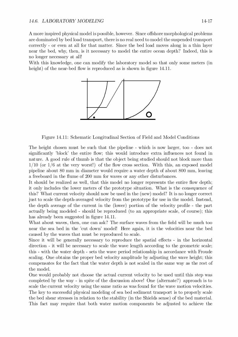
14.6. LABORATORY MODELING 14-17
A more inspired physical model is possible, however. Since o¤shore morphological problemsare dominated by bed load transport, there is no real need to model the suspended transportcorrectly - or even at all for that matter. Since the bed load moves along in a thin layernear the bed, why, then, is it necessary to model the entire ocean depth? Indeed, this isno longer necessary at all!With this knowledge, one can modify the laboratory model so that only some meters (inheight) of the near-bed ‡ow is reproduced as is shown in …gure 14.11.
Figure 14.11: Schematic Longitudinal Section of Field and Model Conditions
The height chosen must be such that the pipeline - which is now larger, too - does notsigni…cantly ’block’ the entire ‡ow; this would introduce extra in‡uences not found innature. A good rule of thumb is that the object being studied should not block more than1=10 (or 1=6 at the very worst!) of the ‡ow cross section. With this, an exposed modelpipeline about 80 mm in diameter would require a water depth of about 800 mm, leavinga freeboard in the ‡ume of 200 mm for waves or any other disturbances.It should be realized as well, that this model no longer represents the entire ‡ow depth;it only includes the lower meters of the prototype situation. What is the consequence ofthis? What current velocity should now be used in the (new) model? It is no longer correctjust to scale the depth-averaged velocity from the prototype for use in the model. Instead,the depth average of the current in the (lower) portion of the velocity pro…le - the partactually being modeled - should be reproduced (to an appropriate scale, of course); thishas already been suggested in …gure 14.11.What about waves, then, one can ask? The surface waves from the …eld will be much toonear the sea bed in the ’cut down’ model! Here again, it is the velocities near the bedcaused by the waves that must be reproduced to scale.Since it will be generally necessary to reproduce the spatial e¤ects - in the horizontaldirection - it will be necessary to scale the wave length according to the geometric scale;this - with the water depth - sets the wave period relationship in accordance with Froudescaling. One obtains the proper bed velocity amplitude by adjusting the wave height; thiscompensates for the fact that the water depth is not scaled in the same way as the rest ofthe model.One would probably not choose the actual current velocity to be used until this step wascompleted by the way - in spite of the discussion above! One (alternate?) approach is toscale the current velocity using the same ratio as was found for the wave motion velocities.The key to successful physical modeling of sea bed sediment transport is to properly scalethe bed shear stresses in relation to the stability (in the Shields sense) of the bed material.This fact may require that both water motion components be adjusted to achieve the
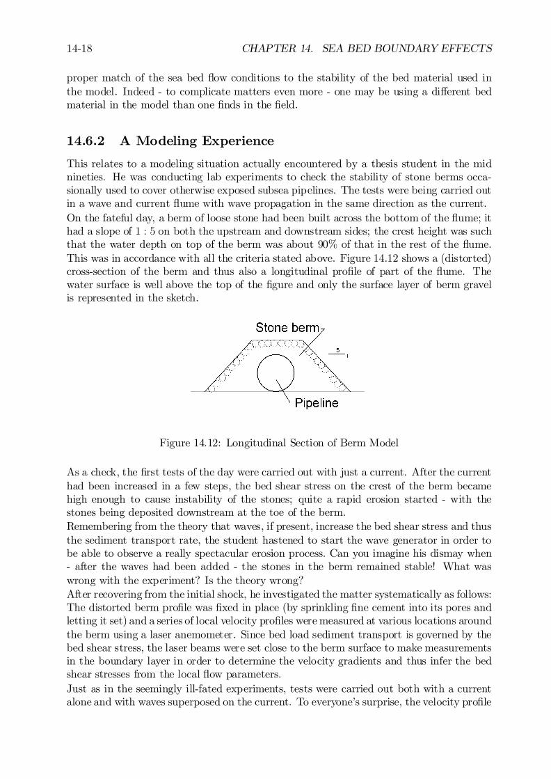
14-18 CHAPTER 14. SEA BED BOUNDARY EFFECTS
proper match of the sea bed ‡ow conditions to the stability of the bed material used inthe model. Indeed - to complicate matters even more - one may be using a di¤erent bedmaterial in the model than one …nds in the …eld.
14.6.2 A Modeling Experience
This relates to a modeling situation actually encountered by a thesis student in the midnineties. He was conducting lab experiments to check the stability of stone berms occa-sionally used to cover otherwise exposed subsea pipelines. The tests were being carried outin a wave and current ‡ume with wave propagation in the same direction as the current.On the fateful day, a berm of loose stone had been built across the bottom of the ‡ume; ithad a slope of 1 : 5 on both the upstream and downstream sides; the crest height was suchthat the water depth on top of the berm was about 90% of that in the rest of the ‡ume.This was in accordance with all the criteria stated above. Figure 14.12 shows a (distorted)cross-section of the berm and thus also a longitudinal pro…le of part of the ‡ume. Thewater surface is well above the top of the …gure and only the surface layer of berm gravelis represented in the sketch.
Figure 14.12: Longitudinal Section of Berm Model
As a check, the …rst tests of the day were carried out with just a current. After the currenthad been increased in a few steps, the bed shear stress on the crest of the berm becamehigh enough to cause instability of the stones; quite a rapid erosion started - with thestones being deposited downstream at the toe of the berm.Remembering from the theory that waves, if present, increase the bed shear stress and thusthe sediment transport rate, the student hastened to start the wave generator in order tobe able to observe a really spectacular erosion process. Can you imagine his dismay when- after the waves had been added - the stones in the berm remained stable! What waswrong with the experiment? Is the theory wrong?After recovering from the initial shock, he investigated the matter systematically as follows:The distorted berm pro…le was …xed in place (by sprinkling …ne cement into its pores andletting it set) and a series of local velocity pro…les were measured at various locations aroundthe berm using a laser anemometer. Since bed load sediment transport is governed by thebed shear stress, the laser beams were set close to the berm surface to make measurementsin the boundary layer in order to determine the velocity gradients and thus infer the bedshear stresses from the local ‡ow parameters.Just as in the seemingly ill-fated experiments, tests were carried out both with a currentalone and with waves superposed on the current. To everyone’s surprise, the velocity pro…le
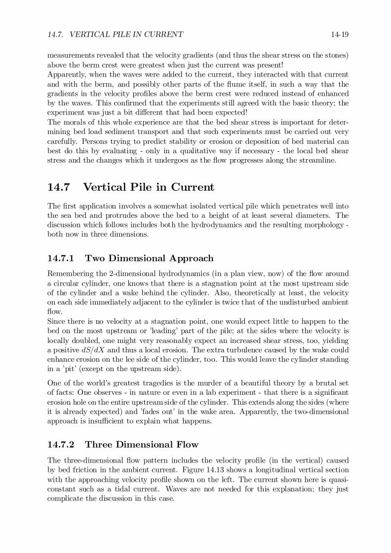
14.7. VERTICAL PILE IN CURRENT 14-19
measurements revealed that the velocity gradients (and thus the shear stress on the stones)above the berm crest were greatest when just the current was present!Apparently, when the waves were added to the current, they interacted with that currentand with the berm, and possibly other parts of the ‡ume itself, in such a way that thegradients in the velocity pro…les above the berm crest were reduced instead of enhancedby the waves. This con…rmed that the experiments still agreed with the basic theory; theexperiment was just a bit di¤erent that had been expected!The morals of this whole experience are that the bed shear stress is important for deter-mining bed load sediment transport and that such experiments must be carried out verycarefully. Persons trying to predict stability or erosion or deposition of bed material canbest do this by evaluating - only in a qualitative way if necessary - the local bed shearstress and the changes which it undergoes as the ‡ow progresses along the streamline.
14.7 Vertical Pile in Current
The …rst application involves a somewhat isolated vertical pile which penetrates well intothe sea bed and protrudes above the bed to a height of at least several diameters. Thediscussion which follows includes both the hydrodynamics and the resulting morphology -both now in three dimensions.
14.7.1 Two Dimensional Approach
Remembering the 2-dimensional hydrodynamics (in a plan view, now) of the ‡ow arounda circular cylinder, one knows that there is a stagnation point at the most upstream sideof the cylinder and a wake behind the cylinder. Also, theoretically at least, the velocityon each side immediately adjacent to the cylinder is twice that of the undisturbed ambient‡ow.Since there is no velocity at a stagnation point, one would expect little to happen to thebed on the most upstream or ’leading’ part of the pile; at the sides where the velocity islocally doubled, one might very reasonably expect an increased shear stress, too, yieldinga positive dS=dX and thus a local erosion. The extra turbulence caused by the wake couldenhance erosion on the lee side of the cylinder, too. This would leave the cylinder standingin a ’pit’ (except on the upstream side).
One of the world’s greatest tragedies is the murder of a beautiful theory by a brutal setof facts: One observes - in nature or even in a lab experiment - that there is a signi…canterosion hole on the entire upstream side of the cylinder. This extends along the sides (whereit is already expected) and ’fades out’ in the wake area. Apparently, the two-dimensionalapproach is insu¢cient to explain what happens.
14.7.2 Three Dimensional Flow
The three-dimensional ‡ow pattern includes the velocity pro…le (in the vertical) causedby bed friction in the ambient current. Figure 14.13 shows a longitudinal vertical sectionwith the approaching velocity pro…le shown on the left. The current shown here is quasi-constant such as a tidal current. Waves are not needed for this explanation; they justcomplicate the discussion in this case.
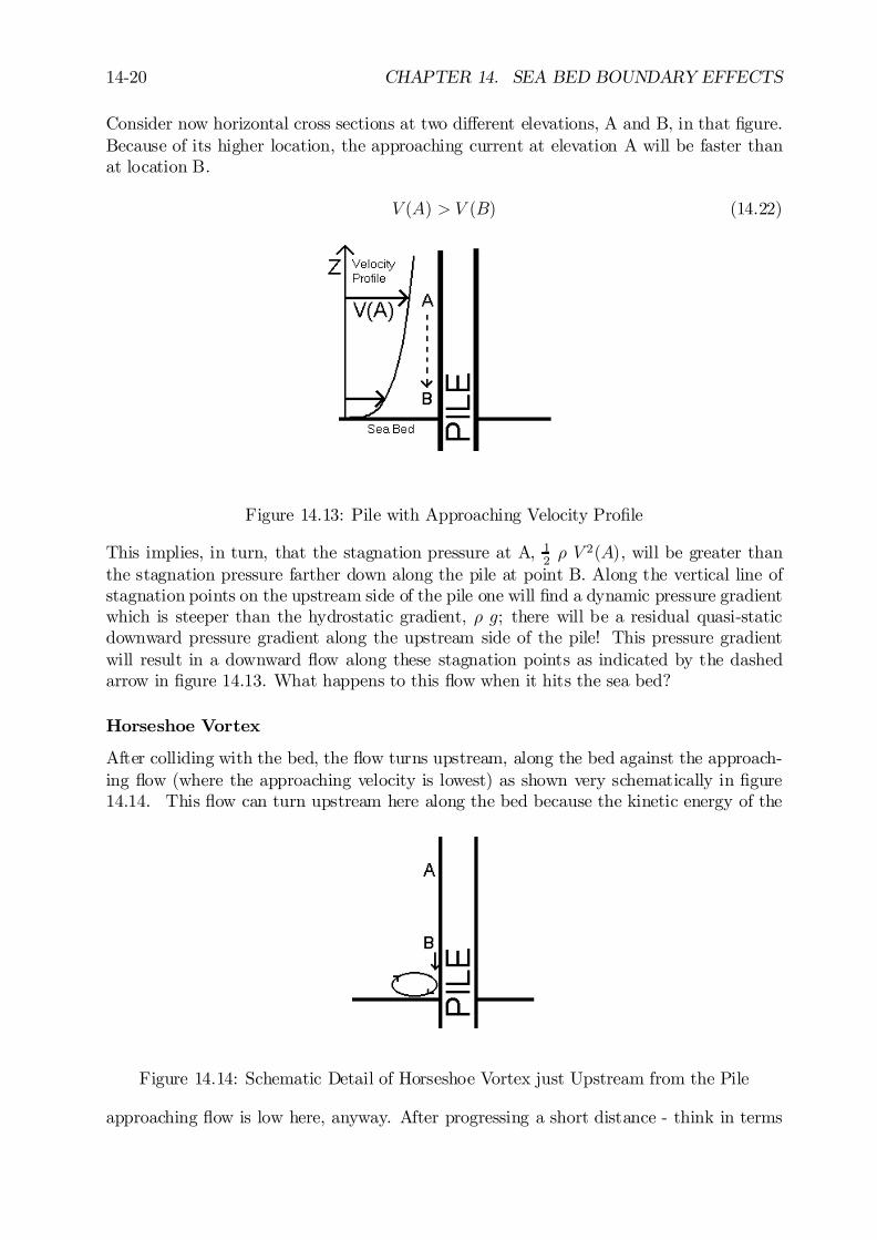
14-20 CHAPTER 14. SEA BED BOUNDARY EFFECTS
Consider now horizontal cross sections at two di¤erent elevations, A and B, in that …gure.Because of its higher location, the approaching current at elevation A will be faster thanat location B.
V (A) > V (B) (14.22)
Figure 14.13: Pile with Approaching Velocity Pro…le
This implies, in turn, that the stagnation pressure at A, 12½ V 2(A), will be greater than
the stagnation pressure farther down along the pile at point B. Along the vertical line ofstagnation points on the upstream side of the pile one will …nd a dynamic pressure gradientwhich is steeper than the hydrostatic gradient, ½ g; there will be a residual quasi-staticdownward pressure gradient along the upstream side of the pile! This pressure gradientwill result in a downward ‡ow along these stagnation points as indicated by the dashedarrow in …gure 14.13. What happens to this ‡ow when it hits the sea bed?
Horseshoe Vortex
After colliding with the bed, the ‡ow turns upstream, along the bed against the approach-ing ‡ow (where the approaching velocity is lowest) as shown very schematically in …gure14.14. This ‡ow can turn upstream here along the bed because the kinetic energy of the
Figure 14.14: Schematic Detail of Horseshoe Vortex just Upstream from the Pile
approaching ‡ow is low here, anyway. After progressing a short distance - think in terms
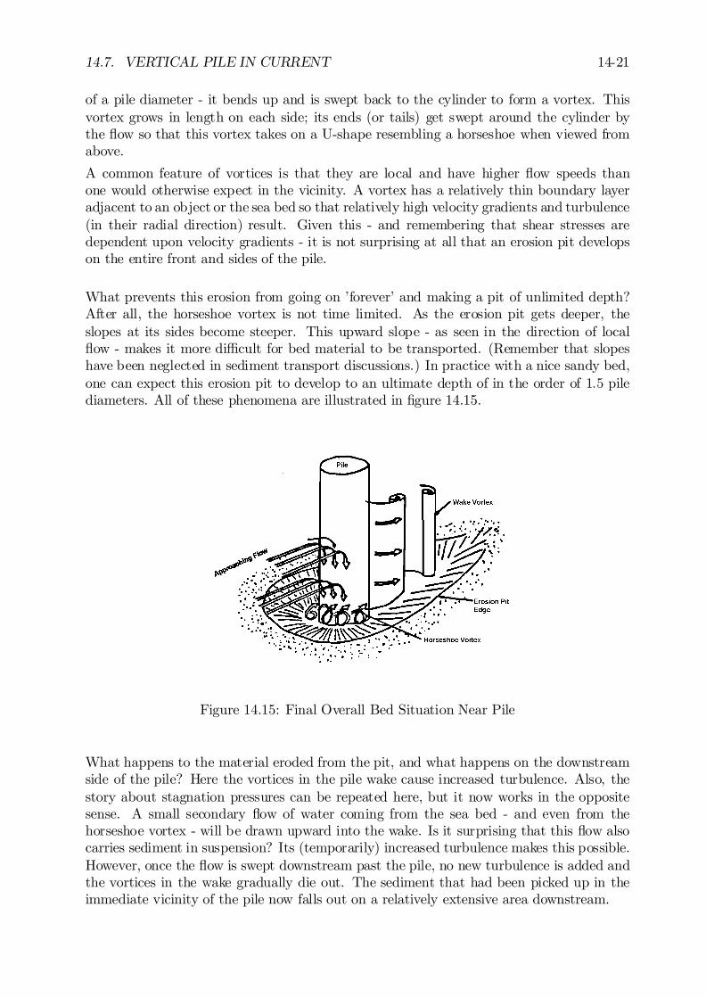
14.7. VERTICAL PILE IN CURRENT 14-21
of a pile diameter - it bends up and is swept back to the cylinder to form a vortex. Thisvortex grows in length on each side; its ends (or tails) get swept around the cylinder bythe ‡ow so that this vortex takes on a U-shape resembling a horseshoe when viewed fromabove.
A common feature of vortices is that they are local and have higher ‡ow speeds thanone would otherwise expect in the vicinity. A vortex has a relatively thin boundary layeradjacent to an object or the sea bed so that relatively high velocity gradients and turbulence(in their radial direction) result. Given this - and remembering that shear stresses aredependent upon velocity gradients - it is not surprising at all that an erosion pit developson the entire front and sides of the pile.
What prevents this erosion from going on ’forever’ and making a pit of unlimited depth?After all, the horseshoe vortex is not time limited. As the erosion pit gets deeper, theslopes at its sides become steeper. This upward slope - as seen in the direction of local‡ow - makes it more di¢cult for bed material to be transported. (Remember that slopeshave been neglected in sediment transport discussions.) In practice with a nice sandy bed,one can expect this erosion pit to develop to an ultimate depth of in the order of 1:5 pilediameters. All of these phenomena are illustrated in …gure 14.15.
Figure 14.15: Final Overall Bed Situation Near Pile
What happens to the material eroded from the pit, and what happens on the downstreamside of the pile? Here the vortices in the pile wake cause increased turbulence. Also, thestory about stagnation pressures can be repeated here, but it now works in the oppositesense. A small secondary ‡ow of water coming from the sea bed - and even from thehorseshoe vortex - will be drawn upward into the wake. Is it surprising that this ‡ow alsocarries sediment in suspension? Its (temporarily) increased turbulence makes this possible.However, once the ‡ow is swept downstream past the pile, no new turbulence is added andthe vortices in the wake gradually die out. The sediment that had been picked up in theimmediate vicinity of the pile now falls out on a relatively extensive area downstream.
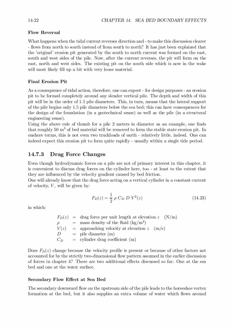
14-22 CHAPTER 14. SEA BED BOUNDARY EFFECTS
Flow Reversal
What happens when the tidal current reverses direction and - to make this discussion clearer- ‡ows from north to south instead of from south to north? It has just been explained thatthe ’original’ erosion pit generated by the south to north current was formed on the east,south and west sides of the pile. Now, after the current reverses, the pit will form on theeast, north and west sides. The existing pit on the south side which is now in the wakewill most likely …ll up a bit with very loose material.
Final Erosion Pit
As a consequence of tidal action, therefore, one can expect - for design purposes - an erosionpit to be formed completely around any slender vertical pile. The depth and width of thispit will be in the order of 1:5 pile diameters. This, in turn, means that the lateral supportof the pile begins only 1:5 pile diameters below the sea bed; this can have consequences forthe design of the foundation (in a geotechnical sense) as well as the pile (in a structuralengineering sense).Using the above rule of thumb for a pile 2 meters in diameter as an example, one …ndsthat roughly 50 m3 of bed material will be removed to form the stable state erosion pit. Inonshore terms, this is not even two truckloads of earth - relatively little, indeed. One canindeed expect this erosion pit to form quite rapidly - usually within a single tide period.
14.7.3 Drag Force Changes
Even though hydrodynamic forces on a pile are not of primary interest in this chapter, itis convenient to discuss drag forces on the cylinder here, too - at least to the extent thatthey are in‡uenced by the velocity gradient caused by bed friction.One will already know that the drag force acting on a vertical cylinder in a constant currentof velocity, V , will be given by:
FD(z) =1
2½ CD D V 2(z) (14.23)
in which:
FD(z) = drag force per unit length at elevation z (N/m)½ = mass density of the ‡uid (kg/m3)V (z) = approaching velocity at elevation z (m/s)D = pile diameter (m)CD = cylinder drag coe¢cient (m)
Does FD(z) change because the velocity pro…le is present or because of other factors notaccounted for by the strictly two-dimensional ‡ow pattern assumed in the earlier discussionof forces in chapter 4? There are two additional e¤ects discussed so far: One at the seabed and one at the water surface.
Secondary Flow E¤ect at Sea Bed
The secondary downward ‡ow on the upstream side of the pile leads to the horseshoe vortexformation at the bed, but it also supplies an extra volume of water which ‡ows around
14.7. VERTICAL PILE IN CURRENT 14-23
the cylinder at the bed elevation. Looked at in another way, the ‡ow past the cylindernear the bed is actually greater than one would expect to …nd based upon the undisturbedapproach velocity at that level.Since the (measured) force is generally related to a velocity which in fact is smaller thanone would associate with that actually present, one will …nd a slightly larger value for thedrag coe¢cient, CD. A plot of CD versus depth will increase a few percent near the seabed.
Water Surface E¤ect
The pile will cause what looks like a standing wave at the water surface. It is in fact atravelling wave which propagates upstream at a speed identical to that of the ‡ow at thatlevel. In this way, the wave stays synchronized with the pile location. This small wavegenerates a dynamic pressure …eld which dies out exponentially with depth (just like thatof any other short wave). Since the wave crest (with higher pressure) is near the upstreampart of the pile and the wave trough (with lower pressure) is on the downstream side, thiswave will cause a net (additional) force component in the direction of the ‡ow.When the total drag force at this level (including this additional component) is related tothe undisturbed near-surface ‡ow velocity, it is only logical that the associated CD valuewill be a few percent higher at this elevation.
Free End E¤ect
A third e¤ect is more often encountered in the lab. One simple way to measure drag forcesin a towing tank is to extend a cylinder vertically downward into a towing tank and to towit while measuring its total resistance as a function of towing velocity. The force is thenassumed to be uniformly distributed over the submerged length of the cylinder in order toultimately arrive at a CD value. Is this correct?This will not be precisely correct for the following two reasons: The force will be disturbed(slightly) by the surface wave already discussed above, and there will be a three-dimensional‡ow pattern near the free, submerged end of the cylinder. This end e¤ect will reduce theforce there.
None of these force disturbances are signi…cant enough for one to have to worry aboutthem when predicting loads on an o¤shore structure. The situation can be quite di¤erentif one is determining a drag coe¢cient value from experiments in the lab, however.These end e¤ects - as all three of these phenomena are sometimes collectively called - canbe eliminated for tests with currents only by adding thin but rigid horizontal plates to thecylinder: One just below the water surface and one near its free end. The upper plateshould be larger than the wave length of the surface disturbance wave; the top of this platewill absorb the wave’s dynamic pressure, thus preventing it from disturbing the pressure…eld lower down in the water. The lower plate will force the ‡ow around the cylinder aboveit to remain two-dimensional.Obviously, it would be best if the drag force was measured now only on some segment- located between the two guiding plates - of the total cylinder length. If this is done,however, and the measuring section is far enough from the water surface and the free endanyway, then it is not necessary to install the ‡ow-guiding plates in the …rst place.
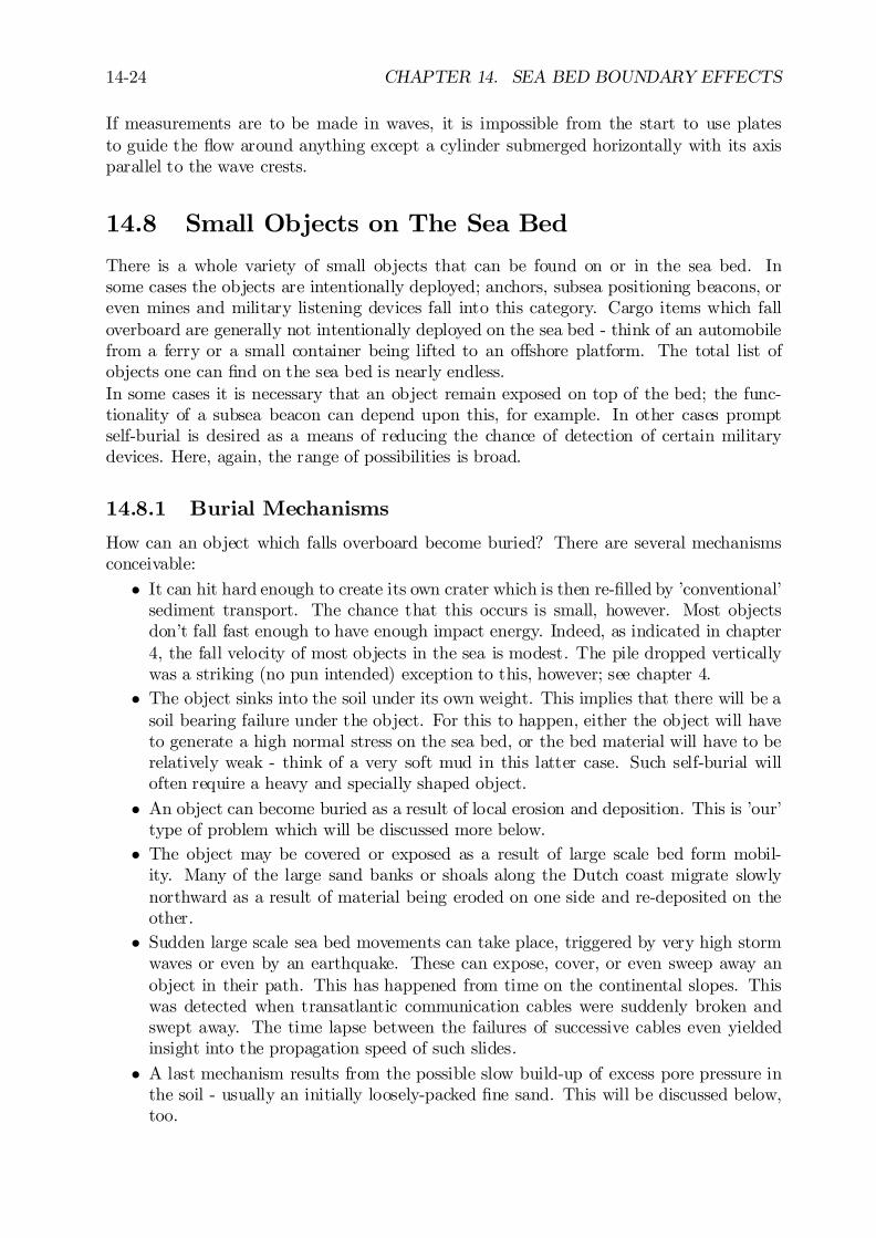
14-24 CHAPTER 14. SEA BED BOUNDARY EFFECTS
If measurements are to be made in waves, it is impossible from the start to use platesto guide the ‡ow around anything except a cylinder submerged horizontally with its axisparallel to the wave crests.
14.8 Small Objects on The Sea Bed
There is a whole variety of small objects that can be found on or in the sea bed. Insome cases the objects are intentionally deployed; anchors, subsea positioning beacons, oreven mines and military listening devices fall into this category. Cargo items which falloverboard are generally not intentionally deployed on the sea bed - think of an automobilefrom a ferry or a small container being lifted to an o¤shore platform. The total list ofobjects one can …nd on the sea bed is nearly endless.In some cases it is necessary that an object remain exposed on top of the bed; the func-tionality of a subsea beacon can depend upon this, for example. In other cases promptself-burial is desired as a means of reducing the chance of detection of certain militarydevices. Here, again, the range of possibilities is broad.
14.8.1 Burial Mechanisms
How can an object which falls overboard become buried? There are several mechanismsconceivable:
² It can hit hard enough to create its own crater which is then re-…lled by ’conventional’sediment transport. The chance that this occurs is small, however. Most objectsdon’t fall fast enough to have enough impact energy. Indeed, as indicated in chapter4, the fall velocity of most objects in the sea is modest. The pile dropped verticallywas a striking (no pun intended) exception to this, however; see chapter 4.
² The object sinks into the soil under its own weight. This implies that there will be asoil bearing failure under the object. For this to happen, either the object will haveto generate a high normal stress on the sea bed, or the bed material will have to berelatively weak - think of a very soft mud in this latter case. Such self-burial willoften require a heavy and specially shaped object.
² An object can become buried as a result of local erosion and deposition. This is ’our’type of problem which will be discussed more below.
² The object may be covered or exposed as a result of large scale bed form mobil-ity. Many of the large sand banks or shoals along the Dutch coast migrate slowlynorthward as a result of material being eroded on one side and re-deposited on theother.
² Sudden large scale sea bed movements can take place, triggered by very high stormwaves or even by an earthquake. These can expose, cover, or even sweep away anobject in their path. This has happened from time on the continental slopes. Thiswas detected when transatlantic communication cables were suddenly broken andswept away. The time lapse between the failures of successive cables even yieldedinsight into the propagation speed of such slides.
² A last mechanism results from the possible slow build-up of excess pore pressure inthe soil - usually an initially loosely-packed …ne sand. This will be discussed below,too.
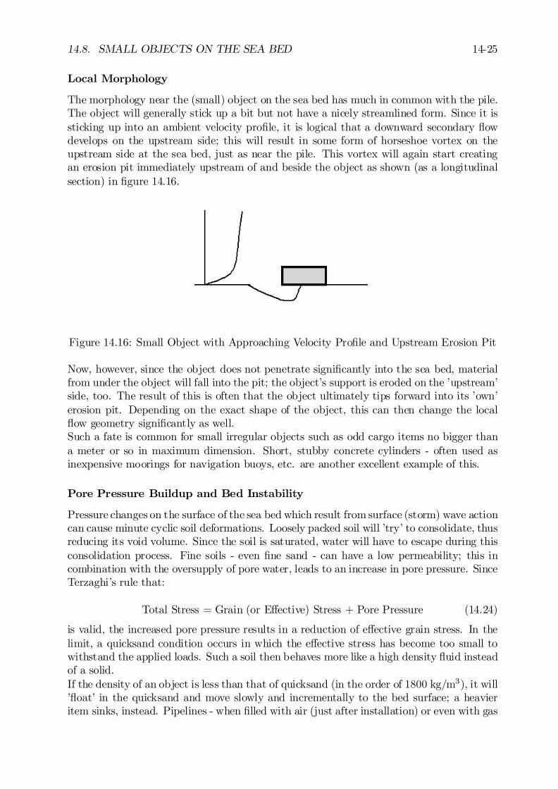
14.8. SMALL OBJECTS ON THE SEA BED 14-25
Local Morphology
The morphology near the (small) object on the sea bed has much in common with the pile.The object will generally stick up a bit but not have a nicely streamlined form. Since it issticking up into an ambient velocity pro…le, it is logical that a downward secondary ‡owdevelops on the upstream side; this will result in some form of horseshoe vortex on theupstream side at the sea bed, just as near the pile. This vortex will again start creatingan erosion pit immediately upstream of and beside the object as shown (as a longitudinalsection) in …gure 14.16.
Figure 14.16: Small Object with Approaching Velocity Pro…le and Upstream Erosion Pit
Now, however, since the object does not penetrate signi…cantly into the sea bed, materialfrom under the object will fall into the pit; the object’s support is eroded on the ’upstream’side, too. The result of this is often that the object ultimately tips forward into its ’own’erosion pit. Depending on the exact shape of the object, this can then change the local‡ow geometry signi…cantly as well.Such a fate is common for small irregular objects such as odd cargo items no bigger thana meter or so in maximum dimension. Short, stubby concrete cylinders - often used asinexpensive moorings for navigation buoys, etc. are another excellent example of this.
Pore Pressure Buildup and Bed Instability
Pressure changes on the surface of the sea bed which result from surface (storm) wave actioncan cause minute cyclic soil deformations. Loosely packed soil will ’try’ to consolidate, thusreducing its void volume. Since the soil is saturated, water will have to escape during thisconsolidation process. Fine soils - even …ne sand - can have a low permeability; this incombination with the oversupply of pore water, leads to an increase in pore pressure. SinceTerzaghi’s rule that:
Total Stress = Grain (or E¤ective) Stress + Pore Pressure (14.24)
is valid, the increased pore pressure results in a reduction of e¤ective grain stress. In thelimit, a quicksand condition occurs in which the e¤ective stress has become too small towithstand the applied loads. Such a soil then behaves more like a high density ‡uid insteadof a solid.If the density of an object is less than that of quicksand (in the order of 1800 kg/m3), it will’‡oat’ in the quicksand and move slowly and incrementally to the bed surface; a heavieritem sinks, instead. Pipelines - when …lled with air (just after installation) or even with gas
14-26 CHAPTER 14. SEA BED BOUNDARY EFFECTS
often have an overall density of about 1300 kg/m3; they have been known to ’‡oat’ upwardthrough a beach and become re-exposed. At the opposite end of the scale, electric andsome communications cables buried in the ground or sea bed will have an overall densityof more like 4000 kg/m3; they will indeed sink.Note that it is not absolutely necessary for the quicksand condition to become ’fully devel-oped’. The soil’s e¤ective intergranular stress and thus its shear strength is reduced as soonas the pore pressure increases. Since the net vertical force exerted by the buried object - itdoes not matter if it is positive or negative - will also cause shear stresses in the surround-ing soil, it is only necessary that the soil’s shear strength be reduced below the imposedstress level for failure to occur. Actual failure usually occurs slowly, the cyclic wave actionstimulates cyclic variations in the pore pressure so that the failure is intermittent ratherthan continuous.Relatively large pressure cycles are needed in order to build up su¢cient pore pressure forthis whole process to take place; this makes it essentially a shallow water phenomenon inthe marine environment. At leas one newly-installed pipeline has ‡oated up after beingburied across a beach in The Netherlands. Luckily the problem became apparent beforethe pipeline was put into service.In an onshore situation, electric cables laid in poor soil have been ’lost’ in that they havesunk deeper - except where they are held in place in a junction house! In this case, thevibration source was the tra¢c on the adjacent highway.What can be done to prevent this problem - at least in the marine situation? There aretwo possible solution approaches:
1. Consolidate the sand arti…cially as the pipeline or cable trench is being back…lled.While this is theoretically possible, it is probably a pretty expensive solution for apipeline - even when one can work from the beach! Hydraulic engineers have used thisapproach however during the construction of the dam in the mouth of the EasternSchelde. There, they feared that vibrations of the barrier support structures couldlead to pore pressure build-up and subsequent failure of the deeper sand layers.
2. Back…ll the pipeline trench with coarser material, providing su¢cient soil permeabil-ity to prevent pore pressure build-up. This is the most commonly chosen preventativemeasure - at least for o¤shore situations.
14.9 Pipelines
This section discusses forces on exposed pipelines as well as the sea bed morphology intheir vicinity. The discussion of hydrodynamic forces on pipelines has been delayed tillthis point because the presence of the current velocity pro…le caused by bed friction playssuch an important role in the hydrodynamics.A pipeline seems like a small object when seen in cross-section; in the third dimension it isvery much a one-dimensional or line-like object. Much of what was discussed about smallobjects on the sea bed turns out to be applicable to pipeline cross-sections as well. Thereader must be careful, however; since di¤erences do exist. The following discussion will befor a pipeline which is initially laying on the sea bed with only a minimum of penetrationinto that bed (caused by its own weight). The current will ‡ow more or less perpendicularto the pipeline route. The sea bed material is sand.
14.9. PIPELINES 14-27
14.9.1 Flow and Forces
Because the pipeline is bedded slightly in the sand, it will not allow ‡ow to pass under it; theentire approaching ‡ow will have to pass over the pipeline. This ‡ow pattern is obviouslyquite distorted relative to that for an isolated cylinder far away from any ‡ow-constrainingwalls.
Drag Force
The drag coe¢cient for the pipeline will be somewhat higher than that for the cylinderin the unrestricted ‡ow. This higher drag coe¢cient is then used in conjunction with theundisturbed current at the elevation of the pipeline center line. Remember that thereis a strong velocity pro…le gradient here! Continuing the discussion of the horizontalequilibrium, …rst, the drag force is resisted by a friction force which, in turn, depends uponthe contact force between the pipeline and the sea bed; horizontal stability depends uponthe vertical force balance, too. These forces are all illustrated schematically in …gure 14.17.There will be something similar to a stagnation area - with an associated relatively highquasi-static pressure - on the upstream side of the pipe near the bed.
Figure 14.17: Flow Situation and Forces on a Cross Section of Exposed Pipe
Lift Force
Because of the approaching velocity pro…le and the fact that all of the ‡ow must pass overthe pipe, the velocities on top of the pipe will be even higher than those predicted bypotential theory for an isolated cylinder. The concept of re‡ection was used in chapter 3to model a potential ‡ow around a cylinder near (or in contact with) a ‡at bed, but thisstill neglects the in‡uence of the velocity pro…le in the approaching ‡ow.A high velocity along the top of the pipe implies low pressure there, while the water onthe underside of the pipe - near point P in …gure 14.17 - is nearly stagnant.Conceptually, this begins to resemble the net ‡ow e¤ect of an isolated cylinder in a uni-form current and surrounded by a circulation; the net force e¤ect will be a lift directedperpendicular to the current - upward in this case. This force will have to be counteractedby pipe weight.Looking for a moment at the total vertical equilibrium, this lift force reduces the soilcontact force and thus, indirectly, the sliding friction resistance from the bed. Unless thepipe is constrained somewhere else along its length, it will slide sideways before it lifts o¤the bottom.
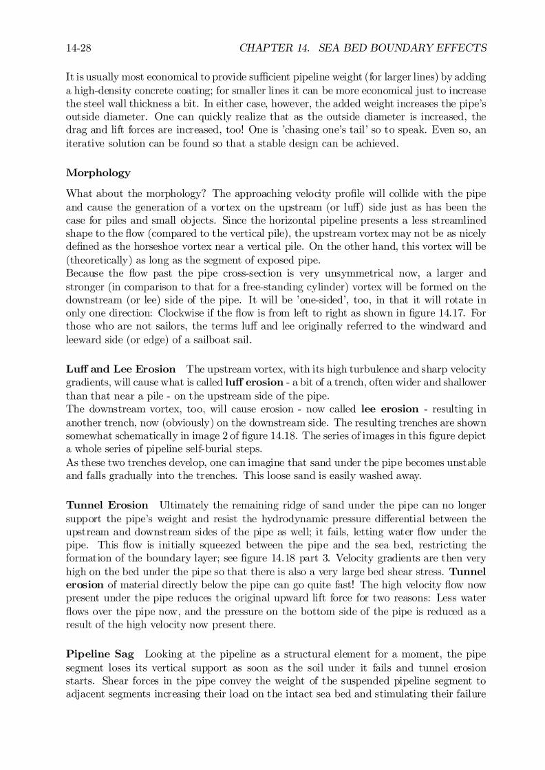
14-28 CHAPTER 14. SEA BED BOUNDARY EFFECTS
It is usually most economical to provide su¢cient pipeline weight (for larger lines) by addinga high-density concrete coating; for smaller lines it can be more economical just to increasethe steel wall thickness a bit. In either case, however, the added weight increases the pipe’soutside diameter. One can quickly realize that as the outside diameter is increased, thedrag and lift forces are increased, too! One is ’chasing one’s tail’ so to speak. Even so, aniterative solution can be found so that a stable design can be achieved.
Morphology
What about the morphology? The approaching velocity pro…le will collide with the pipeand cause the generation of a vortex on the upstream (or lu¤) side just as has been thecase for piles and small objects. Since the horizontal pipeline presents a less streamlinedshape to the ‡ow (compared to the vertical pile), the upstream vortex may not be as nicelyde…ned as the horseshoe vortex near a vertical pile. On the other hand, this vortex will be(theoretically) as long as the segment of exposed pipe.Because the ‡ow past the pipe cross-section is very unsymmetrical now, a larger andstronger (in comparison to that for a free-standing cylinder) vortex will be formed on thedownstream (or lee) side of the pipe. It will be ’one-sided’, too, in that it will rotate inonly one direction: Clockwise if the ‡ow is from left to right as shown in …gure 14.17. Forthose who are not sailors, the terms lu¤ and lee originally referred to the windward andleeward side (or edge) of a sailboat sail.
Lu¤ and Lee Erosion The upstream vortex, with its high turbulence and sharp velocitygradients, will cause what is called lu¤ erosion - a bit of a trench, often wider and shallowerthan that near a pile - on the upstream side of the pipe.The downstream vortex, too, will cause erosion - now called lee erosion - resulting inanother trench, now (obviously) on the downstream side. The resulting trenches are shownsomewhat schematically in image 2 of …gure 14.18. The series of images in this …gure depicta whole series of pipeline self-burial steps.As these two trenches develop, one can imagine that sand under the pipe becomes unstableand falls gradually into the trenches. This loose sand is easily washed away.
Tunnel Erosion Ultimately the remaining ridge of sand under the pipe can no longersupport the pipe’s weight and resist the hydrodynamic pressure di¤erential between theupstream and downstream sides of the pipe as well; it fails, letting water ‡ow under thepipe. This ‡ow is initially squeezed between the pipe and the sea bed, restricting theformation of the boundary layer; see …gure 14.18 part 3. Velocity gradients are then veryhigh on the bed under the pipe so that there is also a very large bed shear stress. Tunnelerosion of material directly below the pipe can go quite fast! The high velocity ‡ow nowpresent under the pipe reduces the original upward lift force for two reasons: Less water‡ows over the pipe now, and the pressure on the bottom side of the pipe is reduced as aresult of the high velocity now present there.
Pipeline Sag Looking at the pipeline as a structural element for a moment, the pipesegment loses its vertical support as soon as the soil under it fails and tunnel erosionstarts. Shear forces in the pipe convey the weight of the suspended pipeline segment toadjacent segments increasing their load on the intact sea bed and stimulating their failure
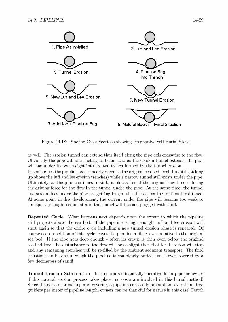
14.9. PIPELINES 14-29
Figure 14.18: Pipeline Cross-Sections showing Progressive Self-Burial Steps
as well. The erosion tunnel can extend thus itself along the pipe axis crosswise to the ‡ow.Obviously the pipe will start acting as beam, and as the erosion tunnel extends, the pipewill sag under its own weight into its own trench formed by the tunnel erosion.In some cases the pipeline axis is nearly down to the original sea bed level (but still stickingup above the lu¤ and lee erosion trenches) while a narrow tunnel still exists under the pipe.Ultimately, as the pipe continues to sink, it blocks less of the original ‡ow thus reducingthe driving force for the ‡ow in the tunnel under the pipe. At the same time, the tunneland streamlines under the pipe are getting longer, thus increasing the frictional resistance.At some point in this development, the current under the pipe will become too weak totransport (enough) sediment and the tunnel will become plugged with sand.
Repeated Cycle What happens next depends upon the extent to which the pipelinestill projects above the sea bed. If the pipeline is high enough, lu¤ and lee erosion willstart again so that the entire cycle including a new tunnel erosion phase is repeated. Ofcourse each repetition of this cycle leaves the pipeline a little lower relative to the originalsea bed. If the pipe gets deep enough - often its crown is then even below the originalsea bed level. Its disturbance to the ‡ow will be so slight then that local erosion will stopand any remaining trenches will be re-…lled by the ambient sediment transport. The …nalsituation can be one in which the pipeline is completely buried and is even covered by afew decimeters of sand!
Tunnel Erosion Stimulation It is of course …nancially lucrative for a pipeline ownerif this natural erosion process takes place; no costs are involved in this burial method!Since the costs of trenching and covering a pipeline can easily amount to several hundredguilders per meter of pipeline length, owners can be thankful for nature in this case! Dutch
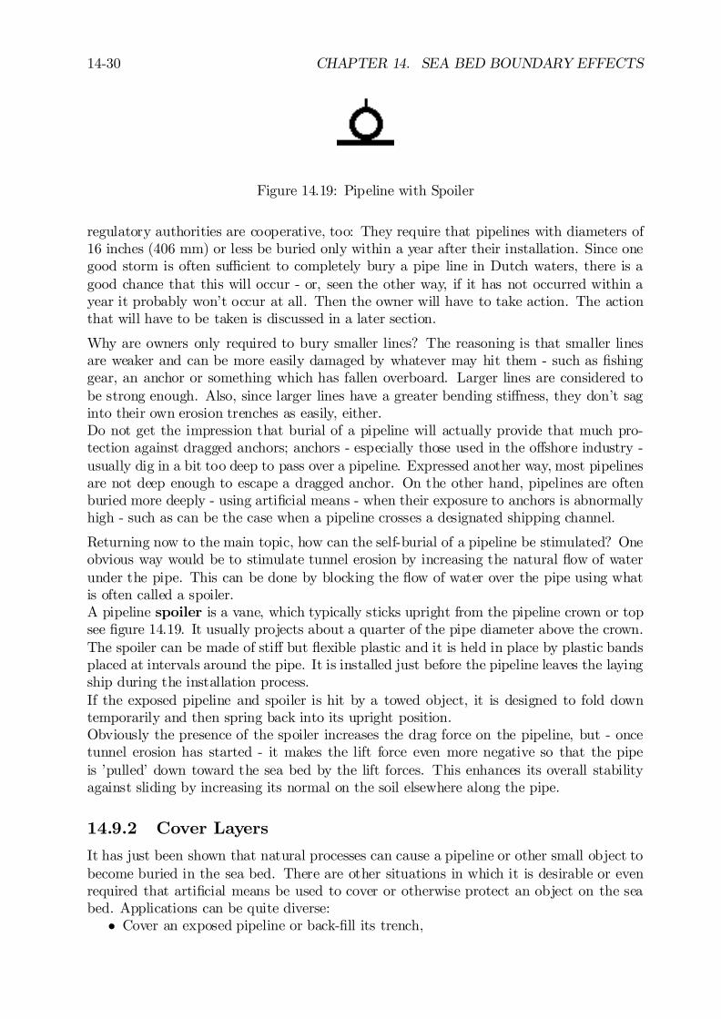
14-30 CHAPTER 14. SEA BED BOUNDARY EFFECTS
Figure 14.19: Pipeline with Spoiler
regulatory authorities are cooperative, too: They require that pipelines with diameters of16 inches (406 mm) or less be buried only within a year after their installation. Since onegood storm is often su¢cient to completely bury a pipe line in Dutch waters, there is agood chance that this will occur - or, seen the other way, if it has not occurred within ayear it probably won’t occur at all. Then the owner will have to take action. The actionthat will have to be taken is discussed in a later section.
Why are owners only required to bury smaller lines? The reasoning is that smaller linesare weaker and can be more easily damaged by whatever may hit them - such as …shinggear, an anchor or something which has fallen overboard. Larger lines are considered tobe strong enough. Also, since larger lines have a greater bending sti¤ness, they don’t saginto their own erosion trenches as easily, either.Do not get the impression that burial of a pipeline will actually provide that much pro-tection against dragged anchors; anchors - especially those used in the o¤shore industry -usually dig in a bit too deep to pass over a pipeline. Expressed another way, most pipelinesare not deep enough to escape a dragged anchor. On the other hand, pipelines are oftenburied more deeply - using arti…cial means - when their exposure to anchors is abnormallyhigh - such as can be the case when a pipeline crosses a designated shipping channel.
Returning now to the main topic, how can the self-burial of a pipeline be stimulated? Oneobvious way would be to stimulate tunnel erosion by increasing the natural ‡ow of waterunder the pipe. This can be done by blocking the ‡ow of water over the pipe using whatis often called a spoiler.A pipeline spoiler is a vane, which typically sticks upright from the pipeline crown or topsee …gure 14.19. It usually projects about a quarter of the pipe diameter above the crown.The spoiler can be made of sti¤ but ‡exible plastic and it is held in place by plastic bandsplaced at intervals around the pipe. It is installed just before the pipeline leaves the layingship during the installation process.If the exposed pipeline and spoiler is hit by a towed object, it is designed to fold downtemporarily and then spring back into its upright position.Obviously the presence of the spoiler increases the drag force on the pipeline, but - oncetunnel erosion has started - it makes the lift force even more negative so that the pipeis ’pulled’ down toward the sea bed by the lift forces. This enhances its overall stabilityagainst sliding by increasing its normal on the soil elsewhere along the pipe.
14.9.2 Cover Layers
It has just been shown that natural processes can cause a pipeline or other small object tobecome buried in the sea bed. There are other situations in which it is desirable or evenrequired that arti…cial means be used to cover or otherwise protect an object on the seabed. Applications can be quite diverse:
² Cover an exposed pipeline or back-…ll its trench,
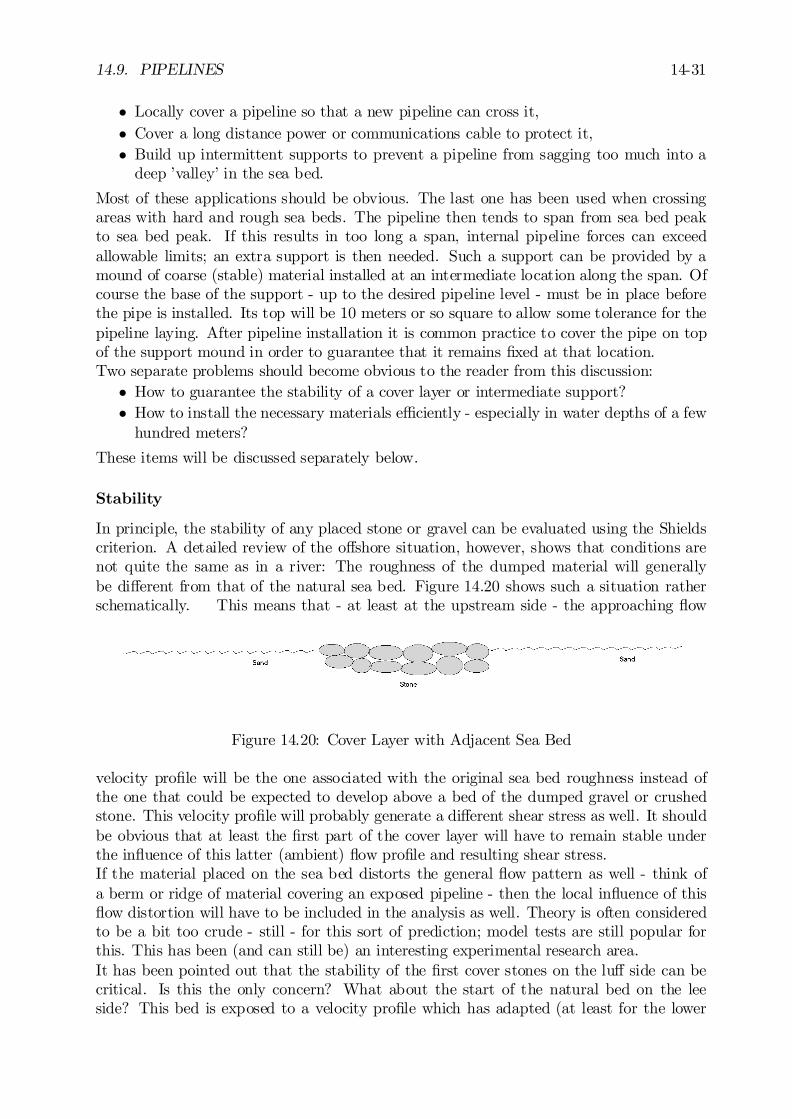
14.9. PIPELINES 14-31
² Locally cover a pipeline so that a new pipeline can cross it,² Cover a long distance power or communications cable to protect it,² Build up intermittent supports to prevent a pipeline from sagging too much into a
deep ’valley’ in the sea bed.
Most of these applications should be obvious. The last one has been used when crossingareas with hard and rough sea beds. The pipeline then tends to span from sea bed peakto sea bed peak. If this results in too long a span, internal pipeline forces can exceedallowable limits; an extra support is then needed. Such a support can be provided by amound of coarse (stable) material installed at an intermediate location along the span. Ofcourse the base of the support - up to the desired pipeline level - must be in place beforethe pipe is installed. Its top will be 10 meters or so square to allow some tolerance for thepipeline laying. After pipeline installation it is common practice to cover the pipe on topof the support mound in order to guarantee that it remains …xed at that location.Two separate problems should become obvious to the reader from this discussion:
² How to guarantee the stability of a cover layer or intermediate support?² How to install the necessary materials e¢ciently - especially in water depths of a few
hundred meters?
These items will be discussed separately below.
Stability
In principle, the stability of any placed stone or gravel can be evaluated using the Shieldscriterion. A detailed review of the o¤shore situation, however, shows that conditions arenot quite the same as in a river: The roughness of the dumped material will generallybe di¤erent from that of the natural sea bed. Figure 14.20 shows such a situation ratherschematically. This means that - at least at the upstream side - the approaching ‡ow
Figure 14.20: Cover Layer with Adjacent Sea Bed
velocity pro…le will be the one associated with the original sea bed roughness instead ofthe one that could be expected to develop above a bed of the dumped gravel or crushedstone. This velocity pro…le will probably generate a di¤erent shear stress as well. It shouldbe obvious that at least the …rst part of the cover layer will have to remain stable underthe in‡uence of this latter (ambient) ‡ow pro…le and resulting shear stress.If the material placed on the sea bed distorts the general ‡ow pattern as well - think ofa berm or ridge of material covering an exposed pipeline - then the local in‡uence of this‡ow distortion will have to be included in the analysis as well. Theory is often consideredto be a bit too crude - still - for this sort of prediction; model tests are still popular forthis. This has been (and can still be) an interesting experimental research area.It has been pointed out that the stability of the …rst cover stones on the lu¤ side can becritical. Is this the only concern? What about the start of the natural bed on the leeside? This bed is exposed to a velocity pro…le which has adapted (at least for the lower
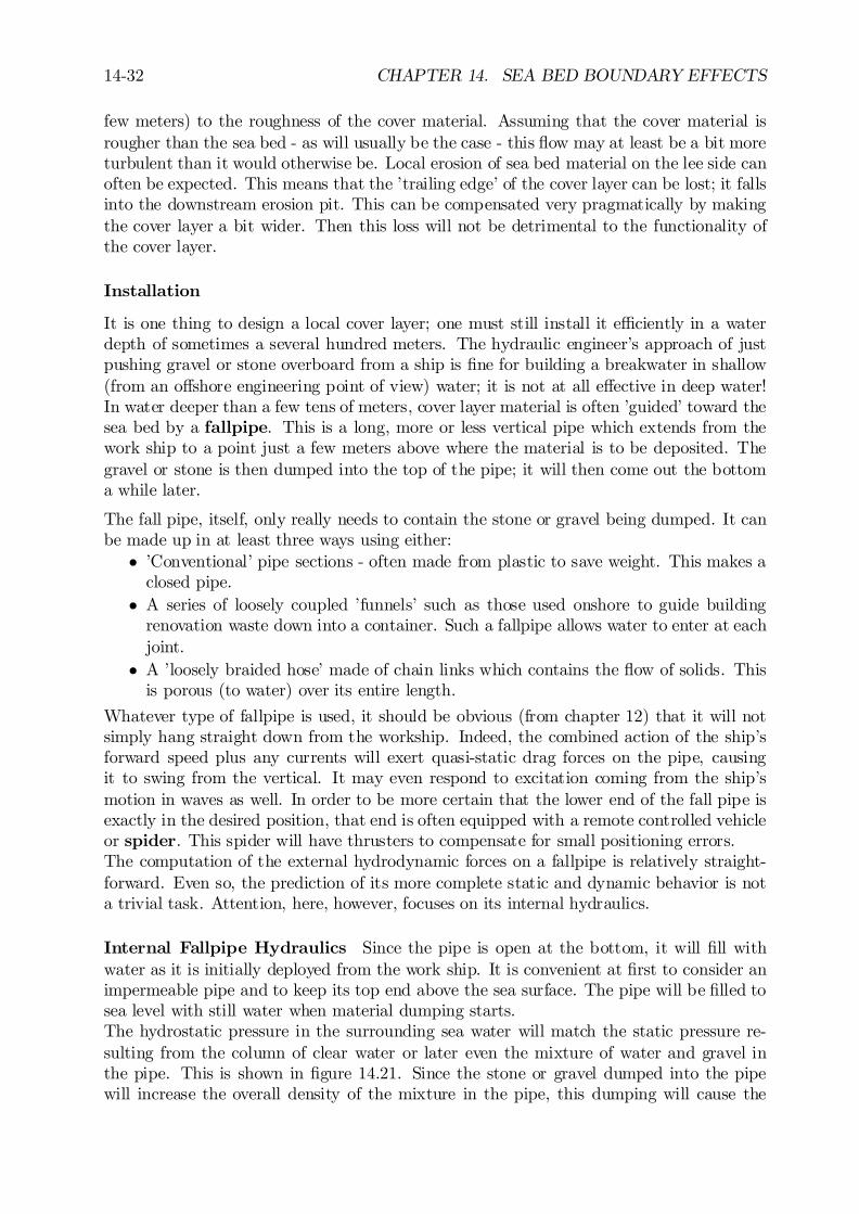
14-32 CHAPTER 14. SEA BED BOUNDARY EFFECTS
few meters) to the roughness of the cover material. Assuming that the cover material isrougher than the sea bed - as will usually be the case - this ‡ow may at least be a bit moreturbulent than it would otherwise be. Local erosion of sea bed material on the lee side canoften be expected. This means that the ’trailing edge’ of the cover layer can be lost; it fallsinto the downstream erosion pit. This can be compensated very pragmatically by makingthe cover layer a bit wider. Then this loss will not be detrimental to the functionality ofthe cover layer.
Installation
It is one thing to design a local cover layer; one must still install it e¢ciently in a waterdepth of sometimes a several hundred meters. The hydraulic engineer’s approach of justpushing gravel or stone overboard from a ship is …ne for building a breakwater in shallow(from an o¤shore engineering point of view) water; it is not at all e¤ective in deep water!In water deeper than a few tens of meters, cover layer material is often ’guided’ toward thesea bed by a fallpipe. This is a long, more or less vertical pipe which extends from thework ship to a point just a few meters above where the material is to be deposited. Thegravel or stone is then dumped into the top of the pipe; it will then come out the bottoma while later.
The fall pipe, itself, only really needs to contain the stone or gravel being dumped. It canbe made up in at least three ways using either:
² ’Conventional’ pipe sections - often made from plastic to save weight. This makes aclosed pipe.
² A series of loosely coupled ’funnels’ such as those used onshore to guide buildingrenovation waste down into a container. Such a fallpipe allows water to enter at eachjoint.
² A ’loosely braided hose’ made of chain links which contains the ‡ow of solids. Thisis porous (to water) over its entire length.
Whatever type of fallpipe is used, it should be obvious (from chapter 12) that it will notsimply hang straight down from the workship. Indeed, the combined action of the ship’sforward speed plus any currents will exert quasi-static drag forces on the pipe, causingit to swing from the vertical. It may even respond to excitation coming from the ship’smotion in waves as well. In order to be more certain that the lower end of the fall pipe isexactly in the desired position, that end is often equipped with a remote controlled vehicleor spider. This spider will have thrusters to compensate for small positioning errors.The computation of the external hydrodynamic forces on a fallpipe is relatively straight-forward. Even so, the prediction of its more complete static and dynamic behavior is nota trivial task. Attention, here, however, focuses on its internal hydraulics.
Internal Fallpipe Hydraulics Since the pipe is open at the bottom, it will …ll withwater as it is initially deployed from the work ship. It is convenient at …rst to consider animpermeable pipe and to keep its top end above the sea surface. The pipe will be …lled tosea level with still water when material dumping starts.The hydrostatic pressure in the surrounding sea water will match the static pressure re-sulting from the column of clear water or later even the mixture of water and gravel inthe pipe. This is shown in …gure 14.21. Since the stone or gravel dumped into the pipewill increase the overall density of the mixture in the pipe, this dumping will cause the
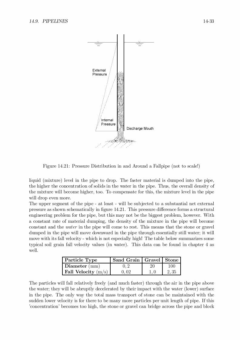
14.9. PIPELINES 14-33
Figure 14.21: Pressure Distribution in and Around a Fallpipe (not to scale!)
liquid (mixture) level in the pipe to drop. The faster material is dumped into the pipe,the higher the concentration of solids in the water in the pipe. Thus, the overall density ofthe mixture will become higher, too. To compensate for this, the mixture level in the pipewill drop even more.The upper segment of the pipe - at least - will be subjected to a substantial net externalpressure as shown schematically in …gure 14.21. This pressure di¤erence forms a structuralengineering problem for the pipe, but this may not be the biggest problem, however. Witha constant rate of material dumping, the density of the mixture in the pipe will becomeconstant and the water in the pipe will come to rest. This means that the stone or graveldumped in the pipe will move downward in the pipe through essentially still water; it willmove with its fall velocity - which is not especially high! The table below summarizes sometypical soil grain fall velocity values (in water). This data can be found in chapter 4 aswell.
Particle Type Sand Grain Gravel StoneDiameter (mm) 0; 2 20 100Fall Velocity (m/s) 0; 02 1; 0 2; 35
The particles will fall relatively freely (and much faster) through the air in the pipe abovethe water; they will be abruptly decelerated by their impact with the water (lower) surfacein the pipe. The only way the total mass transport of stone can be maintained with thesudden lower velocity is for there to be many more particles per unit length of pipe. If this’concentration’ becomes too high, the stone or gravel can bridge across the pipe and block
-34 CHAPTER 14. SEA BED BOUNDARY EFFECTS
it so that nothing more gets through; this is a disaster for the productivity of the entireoperation and embarrassing for the supervisor as well!Even when this is working properly, the particles move relatively slowly - only with theirfall velocity - through the still water in the fallpipe. It would be attractive to increase theproductivity in terms of tons or cubic meters of solid material placed per hour using thesame fallpipe.
One way to increase the productivity of the entire system is to let water ‡ow down thefallpipe along with the stones. Since at any elevation the external hydrostatic pressure isgreater than that in the pipe - see …gure 14.21 - one has only to provide an opening toallow surrounding water to enter. This can be done at chosen intermediate elevations, atthe top only, or even continuously along the pipe. One way to let the water enter is to usea porous pipe - such as the chain links hose - or simply to lower the top end of the pipebelow sea level so that water over‡ows into it at the top.Now, the particles sink through the moving water and a ‡ow of water plus particles isdischarged from the bottom end of the pipe. For the same rate of material supply as wasused with the closed pipe, the concentration of particles discharged will be relatively lowerand the discharge velocity will be higher when water is also moving downward through thefallpipe. Adding water is certainly a simple way to increase the productivity of the system,but how far can one go with this?
Discharge Morphology What can happen when too much water is allowed to enterthe fall pipe? The discharge velocity gets so high that a vertical jet (of a mixture of waterand solids) collides with the sea bed and spreads out. It has even happened that this localspreading current - with its higher density and thin boundary layer! - generates too muchlocal bed shear stress for the material being deposited.. Discharged stone will be sweptaway from the place where it is wanted taking the reputation of the contractor with it!
Another interesting question involves the e¤ect of the grain size distribution of the material.If all of the particles are essentially of the same size and density, then their fall velocitieswill be more or less the same, too. For some applications, such as insulating a hot ‡ow linebetween a subsea well and a production platform, it is desirable to use a well graded gravelto cover the pipe. This reduces the permeability of the cover, thus reducing the heat lossfrom the pipe via convected sea water in its vicinity. (Some crude oils become semi-solidif they are cooled below their so-called pour point temperature; it can be very importantfor the pipeline operator to keep things warm!)When a well graded mixture of gravel sizes is dumped into a fallpipe, then the coarsematerial will fall faster than the …nes. This means that when a discharging operation isstarted, …rst only coarse material will be discharged; there will be a ’tail’ of …nes at theend of the run as well. This need not be important - of itself - for a long pipeline, but itcan make a mess of an attempt to form a neat supporting mound of material by passingslowly back and forth to build it up.A second complication when discharging a well graded mixture of gravel is that the …nestmaterial must remain stable on the sea bed in the discharge jet. Segregation of the particlescan take place so that coarse material is left near the pipeline with the …ner fractionsdeposited more to the sides. This can mean disaster for the insulation function of thecover layer. It has led to litigation between the pipeline owner and covering contractor inthe past.

Appendix A
TABLES
A.1 Greek Symbols
Classic Greek symbols
name letter capital Englishletter pronounciation
alpha ® A ’alpha’beta ¯ B ’vita’gamma ° ¡ ’gama’delta ± ¢ ’delta’epsilon ² , " E ’epsilon’zeta ³ Z ’zita’eta ´ H ’ita’theta # , µ £ ’thita’iota ¶ I ’giota’kappa · K ’kapa’lambda ¸ ¤ ’lambda’mu ¹ M ’mi’nu º N ’ni’xi (”ksi”) » ¥ ’xi’omikron o O ’onikron’pi $ , ¼ ¦ ’pi’rho ½ P ’ro’sigma ¾ § ’sigma’tau ¿ ¨ ’taph’upsilon À Y ’ipsilon’phi ' , Á © ’phi’chi  X ’chi’psi à ª ’psi’omega ! ’omega’
Greek symbols used here
name letter capitalletter
alpha ®beta ¯gamma ° ¡delta ± ¢epsilon "zeta ³eta ´theta µiotakappa ·lambda ¸ ¤mu ¹nu ºxi (”ksi”) »omikronpi ¼ ¦rho ½sigma ¾ §tau ¿ ¨upsilonphi ' , Á ©chi Âpsi à ªomega !
0J.M.J. Journée and W.W. Massie, ”OFFSHORE HYDROMECHANICS”, First Edition, January 2001,Delft University of Technology. For updates see web site: http://www.shipmotions.nl.
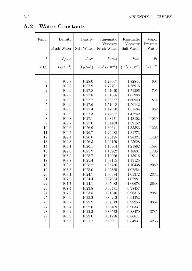
A-2 APPENDIX A. TABLES
A.2 Water Constants
Temp. Density Density Kinematic Kinematic VaporViscosity Viscosity Pressure
Fresh Water Salt Water Fresh Water Salt Water Water
t ½fresh ½salt ºfresh ºsalt pv
(±C) (kg/m3) (kg/m3) (m2s ¢10¡6) (m2s ¢10¡6) (N/m2)
0 999.8 1028.0 1.78667 1.82844 6081 999.8 1027.9 1.72701 1.769152 999.9 1027.8 1.67040 1.71306 7063 999.9 1027.8 1.61665 1.659884 999.9 1027.7 1.56557 1.60940 8145 999.9 1027.6 1.51698 1.561426 999.9 1027.4 1.47070 1.51584 9327 999.8 1027.3 1.42667 1.472428 999.8 1027.1 1.38471 1.43102 10699 999.7 1027.0 1.34463 1.39152
10 999.6 1026.9 1.30641 1.35383 122611 999.5 1026.7 1.26988 1.3177312 999.4 1026.6 1.23495 1.28324 140213 999.3 1026.3 1.20159 1.2502814 999.1 1026.1 1.16964 1.21862 159815 999.0 1025.9 1.13902 1.18831 170616 998.9 1025.7 1.10966 1.15916 181417 998.7 1025.4 1.08155 1.1312518 998.5 1025.2 1.05456 1.10438 205919 998.3 1025.0 1.02865 1.0785420 998.1 1024.7 1.00374 1.05372 233421 997.9 1024.4 0.97984 1.0298122 997.7 1024.1 0.95682 1.00678 263823 997.4 1023.8 0.93471 0.9845724 997.2 1023.5 0.91340 0.96315 298125 996.9 1023.2 0.89292 0.9425226 996.7 1022.9 0.87313 0.92255 336427 996.4 1022.6 0.85409 0.9033128 996.2 1022.3 0.83572 0.88470 378529 995.9 1022.0 0.81798 0.8667130 995.6 1021.7 0.80091 0.84931 4236
Appendix B
MODELING AND MODEL SCALES
B.1 Introduction and Motivations
This appendix provides a rather complete discussion of the design of various sorts of modelsused in o¤shore engineering. Certain speci…c elements - such as Reynolds or Froude scaling,for example - are also summarized in the various chapters of the main text. In its mostabstract sense, a model is some form of representation of an object. In a few cases, it isthe object itself, but it is usually a more convenient representation (in some form) of anactual or proposed situation.Models are used for many purposes; the main reasons for using models include the factsthat they are:
- easier,- faster,- safer,- cheaper.
It is generally easier, faster, safer, and cheaper to work with a model than to make alldiscoveries when a ’real thing’ is used. For example, in the days before Computer AidedDesign (CAD) software became trustworthy, it was common practice to build a plasticmodel of an o¤shore platform topsides - from the design drawings - in order to make surethat the piping all …ts - or even worse - a major structural element con‡icts with the pipingor something else. While such a model may have cost tens of thousands of guilders, it wasobviously much less expensive to correct errors in the design phase rather having to correctthem in the …eld.
B.2 Model Types
There are many types of models that can be used.CAD models in which the form of an object is modeled in a computer have been men-tioned in the example above. Such models are used as well to generate the form of a ship or‡oating structure, for example. Since volumes and weights can easily be calculated, suchsystems can conveniently be extended to interface with hydrodynamic models or to check‡oating stability, for example.
0J.M.J. Journée and W.W. Massie, ”OFFSHORE HYDROMECHANICS”, First Edition, January 2001,Delft University of Technology. For updates see web site: http://www.shipmotions.nl.

B-2 APPENDIX B. MODELING AND MODEL SCALES
Computer Simulations are a special category within the group of Computer Models.These represent the dynamic behavior of an object - such as a ship in waves or even thespreading of an oil spill - e¤ectively by solving the related di¤erential equations.
Computer models - of whatever type - have several advantages, especially in relation totheir alternatives:
² They are reasonably inexpensive to use, although their initial development costs maybe signi…cant.
² Computers are so universally available today that they can be used most anywhere.
² A computer model is safe; they present not danger to humans or the environment.
² All included phenomena can be represented at full scale. (The signifcance of this willbecome apparent below.)
On the other hand, a computer model and especially a simulation has one importantdrawback: it is only as good as the mathematics which is used to (approximately) describethe phenomena which actually take place. In the mid nineteen-eighties, Petroski reportedon the comparison of measured and computed loads in a large transmission line tower.
”Computer predicitions of structural behavior were within only sixty percentof the actual measured values only ninety-…ve percent of the time, ...”
Computer users should never allow blind trust to replace reasonable engineering thinking!
Of course it is possible to carry out testing using a ’real thing’: a full-sized and completeprototype. Such testing can be expensive - certainly if it leads to required changes. Evenwithout that, measuring a ship’s behavior in waves at sea requires a signi…cant mobilizationof test equipment and personnel and one has no control over the input - the weather-dependent waves - either. Many …eld test programs have been unsuccessful because natureprovided the wrong (either too much or too little) input! In some cases it can even bedownright dangerous to carry out measurements on a full-scale basis.This is not to say that prototype testing is always bad; indeed not. Such measurementscan be very valuable as well for diagnostic purposes such as to determine why relativelymany persons on a particular platform complain of motion sickness. Field measurementsare often used as well to verify the correctness of a di¤erent model - of whatever type.Indeed, all physical phenomena are (obviously) properly modeled in a full-scale prototypesituation.
One way to avoid the disadvantages of a (series of) prototype(s) is to use a small scaledmodel and test it in a laboratory instead. Such a model is obviously cheaper than aprototype and the laboratory conditions under which it is tested can be carefully controlled.There is seldom risk to life and limb involved either!Compared to a computer model, a physical model is slower in use but it has at least thepotential to work with a more accurate representation of nature. Indeed, more of the actualphysical phenomena are inherently included in a physical model.A disadvantage of a physical model, however, is that a specialized (and therefore scarceand expensive) test faciltiy is often needed in order to carry out its testing.
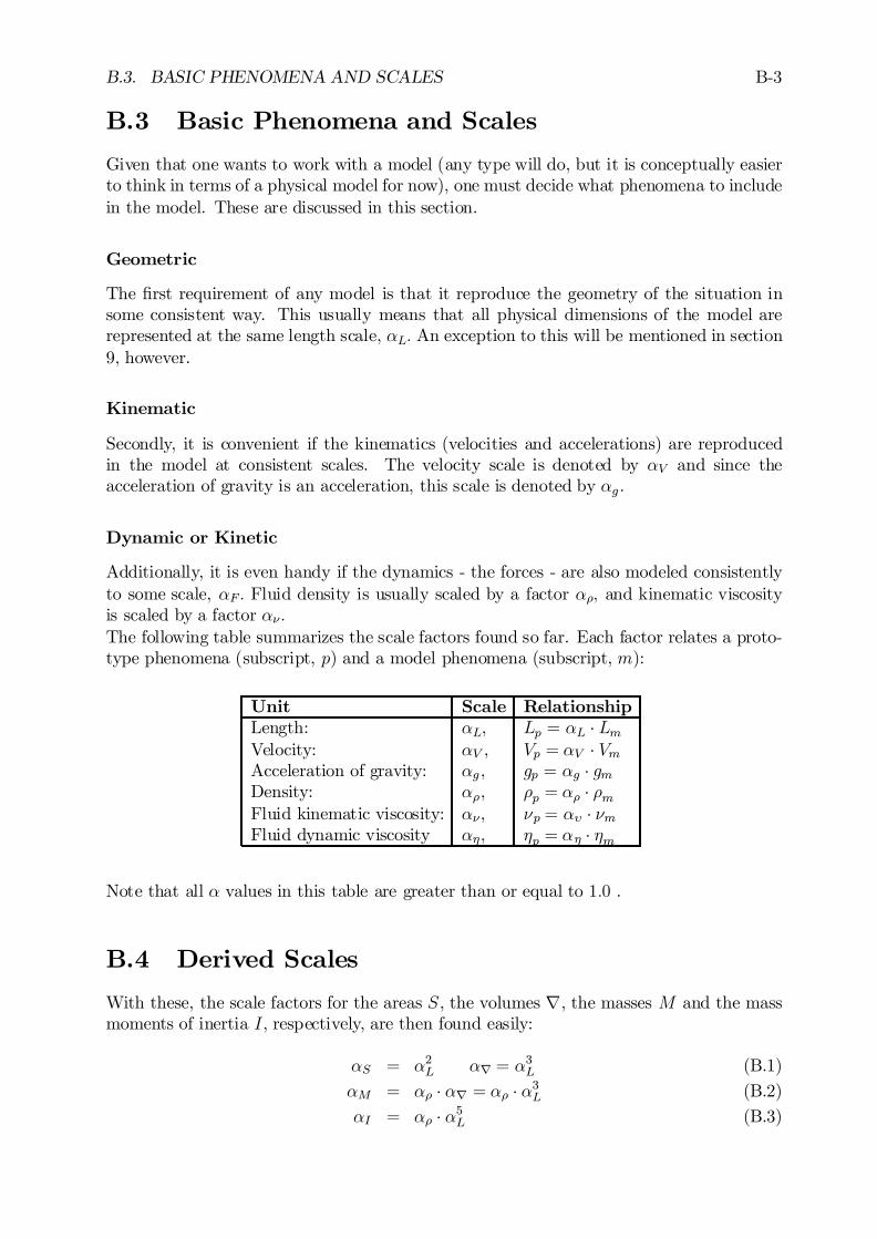
B.3. BASIC PHENOMENA AND SCALES B-3
B.3 Basic Phenomena and Scales
Given that one wants to work with a model (any type will do, but it is conceptually easierto think in terms of a physical model for now), one must decide what phenomena to includein the model. These are discussed in this section.
Geometric
The …rst requirement of any model is that it reproduce the geometry of the situation insome consistent way. This usually means that all physical dimensions of the model arerepresented at the same length scale, ®L: An exception to this will be mentioned in section9, however.
Kinematic
Secondly, it is convenient if the kinematics (velocities and accelerations) are reproducedin the model at consistent scales. The velocity scale is denoted by ®V and since theacceleration of gravity is an acceleration, this scale is denoted by ®g :
Dynamic or Kinetic
Additionally, it is even handy if the dynamics - the forces - are also modeled consistentlyto some scale, ®F : Fluid density is usually scaled by a factor ®½; and kinematic viscosityis scaled by a factor ®º:The following table summarizes the scale factors found so far. Each factor relates a proto-type phenomena (subscript, p) and a model phenomena (subscript, m):
Unit Scale RelationshipLength: ®L, Lp = ®L ¢ LmVelocity: ®V , Vp = ®V ¢ VmAcceleration of gravity: ®g , gp = ®g ¢ gmDensity: ®½, ½p = ®½ ¢ ½mFluid kinematic viscosity: ®º, ºp = ®À ¢ ºmFluid dynamic viscosity ®´, ´p = ®´ ¢ ´m
Note that all ® values in this table are greater than or equal to 1:0 .
B.4 Derived Scales
With these, the scale factors for the areas S , the volumes r, the masses M and the massmoments of inertia I, respectively, are then found easily:
®S = ®2L ®r = ®3L (B.1)
®M = ®½ ¢ ®r = ®½ ¢ ®3L (B.2)
®I = ®½ ¢ ®5L (B.3)
B-4 APPENDIX B. MODELING AND MODEL SCALES
The velocity of a body or a (water) particle is de…ned as a displacement per unit of time,so the scale factor for the time becomes:
®T =®L®V
(B.4)
The acceleration of a body or a (water) particle is de…ned as an increase of the velocityper unit of time, so the scale factor for the acceleration becomes:
®A =®V®T
=®2V®L
(B.5)
This should be same, by the way, as the scale factor for the acceleration of gravity, ®g .According to Newton’s law, inertia forces are de…ned as a product of mass and acceleration,so the scale factor for the inertia forces (and also the resulting pressure forces) is:
®F = ®M ¢ ®A =¡®½ ¢ ®3L
¢¢µ®2V®L
¶= (B.6)
= ®½ ¢ ®2V ¢ ®2L (B.7)
Then, the relation beteen the forces Fp on the prototype and the forces Fm on the modelare:
Fp = ®½ ¢ ®2V ¢ ®2L ¢ Fm (B.8)
or:
®F =FpFm
=½p ¢ V 2p ¢L2p½m ¢ V 2m ¢ L2m
(B.9)
From this, it is obvious that these forces can be expressed as:
Fp = C ¢ 12½pV
2p ¢ L2p and Fm = C ¢ 1
2½mV
2m ¢ L2m (B.10)
in which the coe¢cient or constant C does not depend on the scale. Further, one recognizesthe term 1
2½V 2 as the stagnation pressure.
B.5 Forces to Model
Since forces and kinetic similarity are so important in o¤shore engineering, extra attentionto speci…c forces is given in this section.
Inertia
Whenever velocities and accelerations are involved - and that is the usual case in o¤shoreengineering - modeling will involve inertia forces.
Gravity
Gravity forces are important for problems involving buoyancy and more generally for ‡owsituations in which a free water surface is involved. Gravity forces are therefore importantfor waves and for all sorts of open channel ‡ow. They also play an important part in soilmechanics as well. They are not usually very important, on the other hand, for pipeline‡ow.
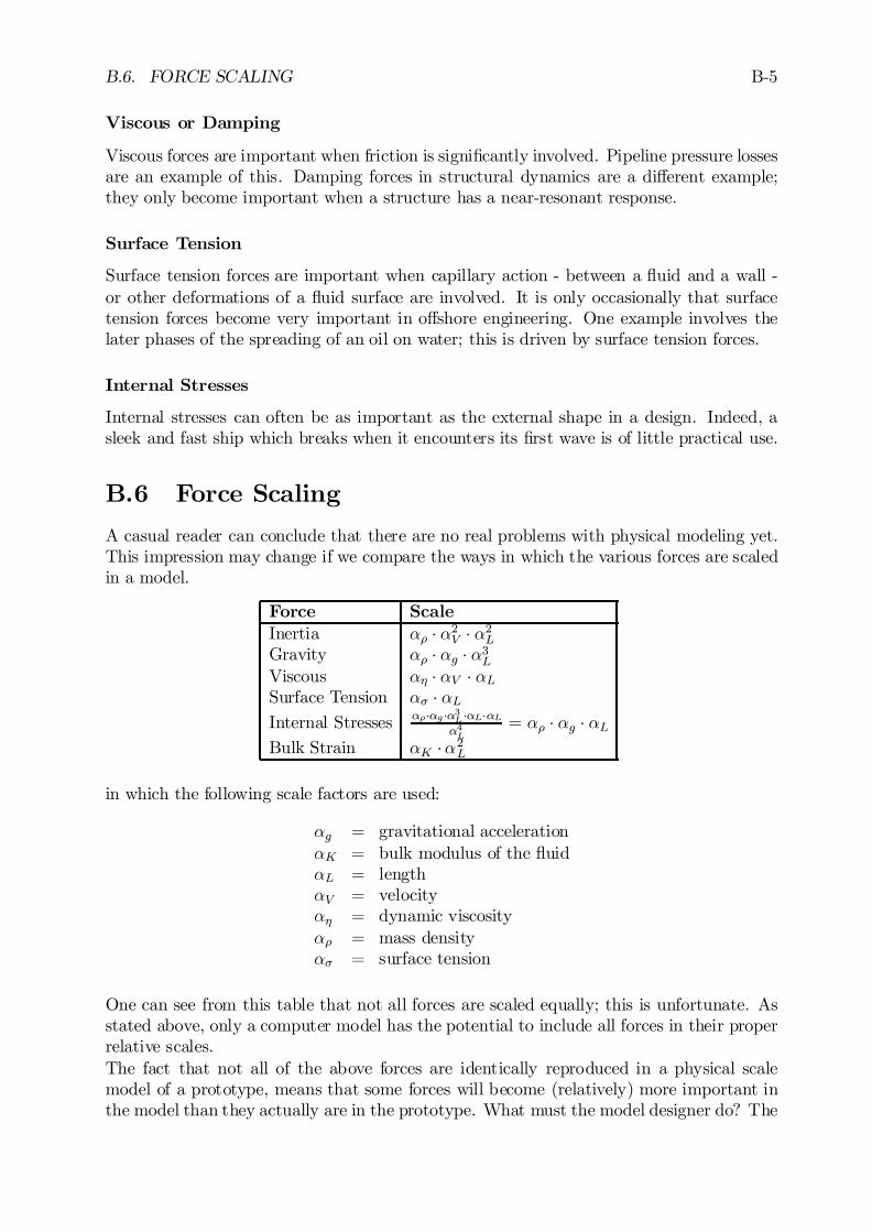
B.6. FORCE SCALING B-5
Viscous or Damping
Viscous forces are important when friction is signi…cantly involved. Pipeline pressure lossesare an example of this. Damping forces in structural dynamics are a di¤erent example;they only become important when a structure has a near-resonant response.
Surface Tension
Surface tension forces are important when capillary action - between a ‡uid and a wall -or other deformations of a ‡uid surface are involved. It is only occasionally that surfacetension forces become very important in o¤shore engineering. One example involves thelater phases of the spreading of an oil on water; this is driven by surface tension forces.
Internal Stresses
Internal stresses can often be as important as the external shape in a design. Indeed, asleek and fast ship which breaks when it encounters its …rst wave is of little practical use.
B.6 Force Scaling
A casual reader can conclude that there are no real problems with physical modeling yet.This impression may change if we compare the ways in which the various forces are scaledin a model.
Force ScaleInertia ®½ ¢ ®2V ¢ ®2LGravity ®½ ¢ ®g ¢ ®3LViscous ®´ ¢ ®V ¢ ®LSurface Tension ®¾ ¢ ®LInternal Stresses ®½¢®g ¢®3L ¢®L¢®L
®4L= ®½ ¢ ®g ¢ ®L
Bulk Strain ®K ¢®2L
in which the following scale factors are used:
®g = gravitational acceleration®K = bulk modulus of the ‡uid®L = length®V = velocity®´ = dynamic viscosity®½ = mass density®¾ = surface tension
One can see from this table that not all forces are scaled equally; this is unfortunate. Asstated above, only a computer model has the potential to include all forces in their properrelative scales.The fact that not all of the above forces are identically reproduced in a physical scalemodel of a prototype, means that some forces will become (relatively) more important inthe model than they actually are in the prototype. What must the model designer do? The
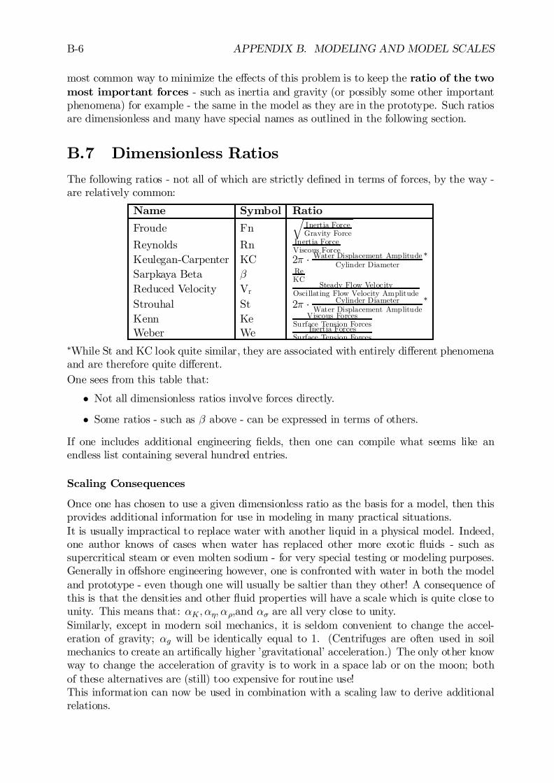
B-6 APPENDIX B. MODELING AND MODEL SCALES
most common way to minimize the e¤ects of this problem is to keep the ratio of the twomost important forces - such as inertia and gravity (or possibly some other importantphenomena) for example - the same in the model as they are in the prototype. Such ratiosare dimensionless and many have special names as outlined in the following section.
B.7 Dimensionless Ratios
The following ratios - not all of which are strictly de…ned in terms of forces, by the way -are relatively common:
Name Symbol Ratio
Froude Fnq
Inertia ForceGravity Force
Reynolds Rn Inertia ForceViscous Force
Keulegan-Carpenter KC 2¼ ¢ Water Displacement AmplitudeCylinder Diameter
¤
Sarpkaya Beta ¯ ReKC
Reduced Velocity VrSteady Flow Velocity
Oscillating Flow Velocity Amplitude
Strouhal St 2¼ ¢ Cylinder DiameterWater Displacement Amplitude
¤
Kenn Ke Viscous ForcesSurface Tension Forces
Weber We Inertia ForcesSurface Tension Forces
¤While St and KC look quite similar, they are associated with entirely di¤erent phenomenaand are therefore quite di¤erent.One sees from this table that:
² Not all dimensionless ratios involve forces directly.
² Some ratios - such as ¯ above - can be expressed in terms of others.
If one includes additional engineering …elds, then one can compile what seems like anendless list containing several hundred entries.
Scaling Consequences
Once one has chosen to use a given dimensionless ratio as the basis for a model, then thisprovides additional information for use in modeling in many practical situations.It is usually impractical to replace water with another liquid in a physical model. Indeed,one author knows of cases when water has replaced other more exotic ‡uids - such assupercritical steam or even molten sodium - for very special testing or modeling purposes.Generally in o¤shore engineering however, one is confronted with water in both the modeland prototype - even though one will usually be saltier than they other! A consequence ofthis is that the densities and other ‡uid properties will have a scale which is quite close tounity. This means that: ®K; ®´; ®½;and ®¾ are all very close to unity.Similarly, except in modern soil mechanics, it is seldom convenient to change the accel-eration of gravity; ®g will be identically equal to 1. (Centrifuges are often used in soilmechanics to create an arti…cally higher ’gravitational’ acceleration.) The only other knowway to change the acceleration of gravity is to work in a space lab or on the moon; bothof these alternatives are (still) too expensive for routine use!This information can now be used in combination with a scaling law to derive additionalrelations.
B.7. DIMENSIONLESS RATIOS B-7
Froude Scaling
Given that the Froude Number in the model must be same as that in the prototype, andthat the Froude Number is the ratio of inertia to gravity forces, one may conclude that -using information from the tables above:
®½ ¢ ®2V ¢ ®2L = ®½ ¢ ®g ¢ ®3L (B.11)
and since:
®V =®L®T
and ®g = 1: (B.12)
then equation B.11 can be re-written as so that:
®L®2T
= 1: (B.13)
Time One can conclude from this that the time scale, ®T =p®L . Thus if a model is
built with a length scale of 100 (1 meter in the prototype is 1 centimeter in the model)then one second in the model will correspond to 10 seconds in the prototype when Froudescaling is used.
Velocity A quick check will show, too, that velocities in the model will also be scaledwith
p®L; a prototype current of 1 m=s will correspond to 10 cm=s in the model.
Reynolds Number and Viscous Forces Since viscous forces may also be involved ina physical model designed to Froude Scale, it can be interesting to check how the ReynoldsNumber is scaled.Since Re is the ratio of inertia to viscous forces, then:
®Re =®½ ¢ ®V ¢ ®L
®´(B.14)
Since ®½ and ®´ are both equal to 1; then ®Re = ®1:5L : This means that the ReynoldsNumber in the model will be 1
1001:5or 1000 times too small. In other words, the viscous
forces in the model will be 1000 times more important in the model than in the …eld.
Keulegan Carpenter Number The Keulegan Carpenter number, KC = uTD , is scaled
according to:
®KC =®V ¢ ®T®L
=
p®L ¢ p
®L®L
´ 1 (B.15)
KC is not changed when Froude scaling is used.
Internal Forces Internal forces - such as bending stresses in the hull of a ship - arescaled according to:®½¢®g ¢®L - from the table above. Since ®½ and ®g are both equal to 1 , then internal stressesare scaled in the same way as the length. Now the example model will be (relatively) 100times as strong as the prototype. Failure to recognize this scaling little detail has led to
B-8 APPENDIX B. MODELING AND MODEL SCALES
the failure (in the …eld) of concrete armor units for rubble mound breakwaters. Concreteunits used in the model were strong enough, but the prototype scale units in the …eld didnot have a signi…cantly higher allowable stress than in the model. As a consequence, theconcrete units in the sea broke up in a storm and the whole breakwater - as well as theinfrastructure it was protecting - was severely damaged.
Reynolds Scaling
One way to avoid the distortion of the viscous forces in a Froude Scale Model is to useReynolds Scaling, instead. Now the ratio of inertia to viscous forces is kept constant. Thismeans that:
®½ ¢ ®2V ¢ ®2L = ®´ ¢ ®V ¢ ®L (B.16)
Since ®½ and ®´ are still equal to 1; then ®V ¢ ®L = 1: so that ®V = 1®L: This means that if
the model has a scale (as above) of 100, then the velocities in the model will have to be 100times larger than in the prototype. This is essentially impossible to achieve in practice!
Other Scaling Laws
Most any of the dimensionless ratios listed in the table above can be used as a basis fora scaling law. Froude Scaling is the most common in o¤shore engineering hydromechanicssimply because gravity plays a dominant role in the behavior of the free surface of theocean. Reynolds scaling is often used for pipe ‡ows (under pressure) such as can be foundin the topsides of an o¤shore production platform.The following …gure compares a variety of scaling laws.
B.8 Practical Compromises
Consider for the moment a physical model of the entire North Sea (to stay o¤shore!) oreven of a few kilometers of a broad river. Since the free water surface is important, Froudescaling would be most appropriate, but one quickly becomes concerned about the stronglyincreased in‡uence of the viscous forces. Indeed, the model can become so shallow thatboundary layer e¤ects become too dominant.
Distorted Scale
One way to reduce the viscous in‡uence in an open channel model is to use a smallerlength scale for vertical dimensions than that used for horizontal dimensions. One authorhas worked on such a model with a vertical scale of 40 and a horizontal scale of 60. Thismakes the model relatively 1.5 times as deep as would be indicated from the …eld. Thiskeeps the Reynolds numbers 1.5 times as large (relative to the undistorted model); theyare still small relative to the prototype or …eld situation, however.
Added Roughness
A quite opposite problem occurs with ship models towed in a towing tank. Because themodels are relatively smooth, the laminar boundary layer which forms near the bow extends
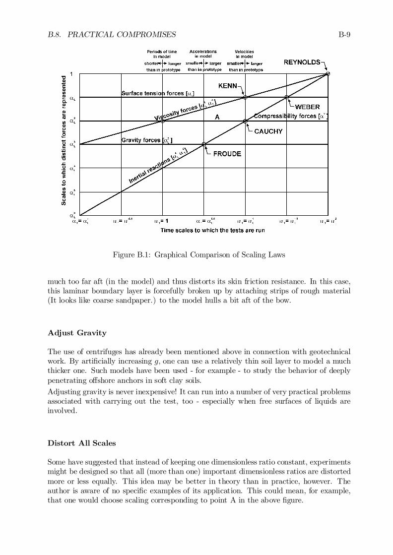
B.8. PRACTICAL COMPROMISES B-9
Figure B.1: Graphical Comparison of Scaling Laws
much too far aft (in the model) and thus distorts its skin friction resistance. In this case,this laminar boundary layer is forcefully broken up by attaching strips of rough material(It looks like coarse sandpaper.) to the model hulls a bit aft of the bow.
Adjust Gravity
The use of centrifuges has already been mentioned above in connection with geotechnicalwork. By arti…cially increasing g; one can use a relatively thin soil layer to model a muchthicker one. Such models have been used - for example - to study the behavior of deeplypenetrating o¤shore anchors in soft clay soils.
Adjusting gravity is never inexpensive! It can run into a number of very practical problemsassociated with carrying out the test, too - especially when free surfaces of liquids areinvolved.
Distort All Scales
Some have suggested that instead of keeping one dimensionless ratio constant, experimentsmight be designed so that all (more than one) important dimensionless ratios are distortedmore or less equally. This idea may be better in theory than in practice, however. Theauthor is aware of no speci…c examples of its application. This could mean, for example,that one would choose scaling corresponding to point A in the above …gure.
B-10 APPENDIX B. MODELING AND MODEL SCALES
B.9 Conclusion
Any physical scale model will distort the relative importance of various forces and otherphysical phenomena involved. On the other hand, a physical model does include all thesephysical phenomena.The only way to avoid the distortions associated with physical models is to use a computermodel or simulation. This has the disadvantage, however, that its representation of thephysical situation is only as good as the mathematician has been able to make it.
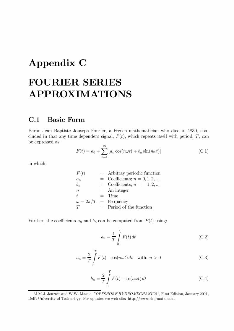
Appendix C
FOURIER SERIESAPPROXIMATIONS
C.1 Basic Form
Baron Jean Baptiste Jouseph Fourier, a French mathematician who died in 1830, con-cluded in that any time dependent signal, F (t), which repeats itself with period, T , canbe expressed as:
F (t) = a0 +1X
n=1
[an cos(n!t) + bn sin(n!t)] (C.1)
in which:
F (t) = Arbitray periodic functionan = Coe¢cients; n = 0; 1; 2; :::bn = Coe¢cients; n = 1; 2; :::n = An integert = Time! = 2¼=T = FrequencyT = Period of the function
Further, the coe¢cients an and bn can be computed from F (t) using:
a0 =1
T
TZ
0
F (t)dt (C.2)
an =2
T
TZ
0
F (t) ¢ cos(n!t)dt with: n > 0 (C.3)
bn =2
T
TZ
0
F (t) ¢ sin(n!t)dt (C.4)
0J.M.J. Journée and W.W. Massie, ”OFFSHORE HYDROMECHANICS”, First Edition, January 2001,Delft University of Technology. For updates see web site: http://www.shipmotions.nl.
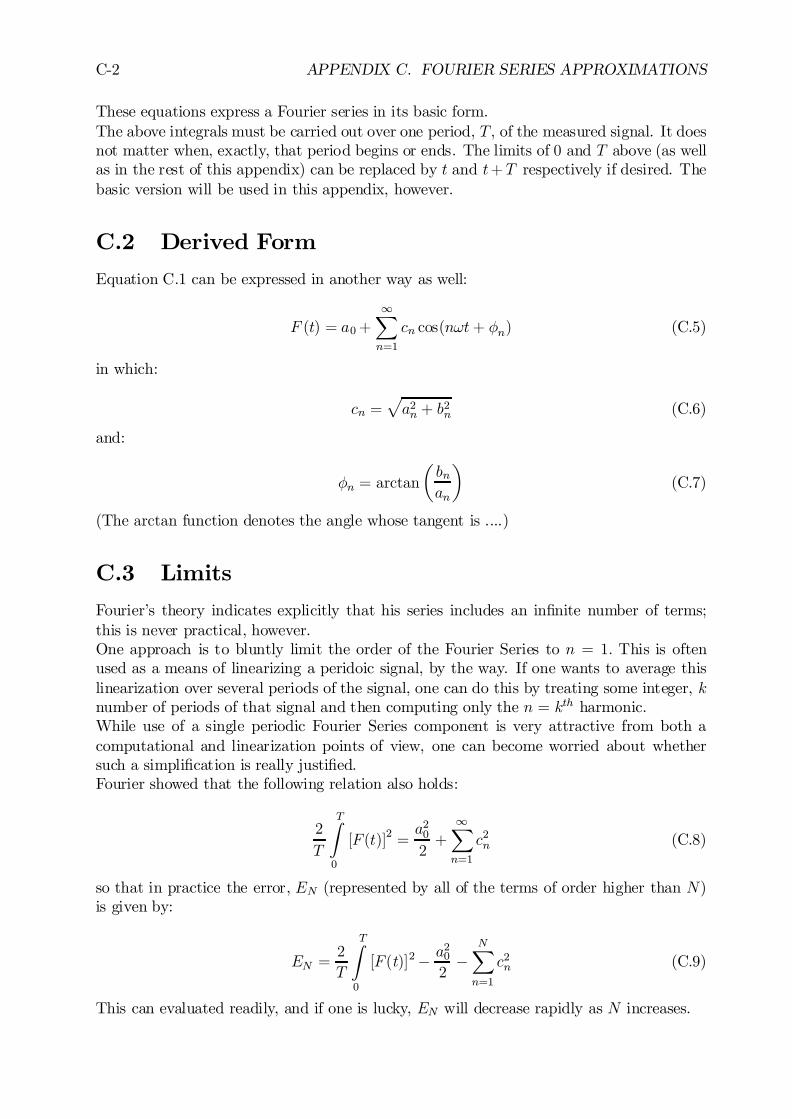
C-2 APPENDIX C. FOURIER SERIES APPROXIMATIONS
These equations express a Fourier series in its basic form.The above integrals must be carried out over one period, T , of the measured signal. It doesnot matter when, exactly, that period begins or ends. The limits of 0 and T above (as wellas in the rest of this appendix) can be replaced by t and t+ T respectively if desired. Thebasic version will be used in this appendix, however.
C.2 Derived Form
Equation C.1 can be expressed in another way as well:
F (t) = a0+1X
n=1
cn cos(n!t+ Án) (C.5)
in which:
cn =pa2n + b
2n (C.6)
and:
Án = arctan
µbnan
¶(C.7)
(The arctan function denotes the angle whose tangent is ....)
C.3 Limits
Fourier’s theory indicates explicitly that his series includes an in…nite number of terms;this is never practical, however.One approach is to bluntly limit the order of the Fourier Series to n = 1: This is oftenused as a means of linearizing a peridoic signal, by the way. If one wants to average thislinearization over several periods of the signal, one can do this by treating some integer, knumber of periods of that signal and then computing only the n = kth harmonic.While use of a single periodic Fourier Series component is very attractive from both acomputational and linearization points of view, one can become worried about whethersuch a simpli…cation is really justi…ed.Fourier showed that the following relation also holds:
2
T
TZ
0
[F (t)]2 =a202+
1X
n=1
c2n (C.8)
so that in practice the error, EN (represented by all of the terms of order higher than N)is given by:
EN =2
T
TZ
0
[F (t)]2¡ a202
¡NX
n=1
c2n (C.9)
This can evaluated readily, and if one is lucky, EN will decrease rapidly as N increases.
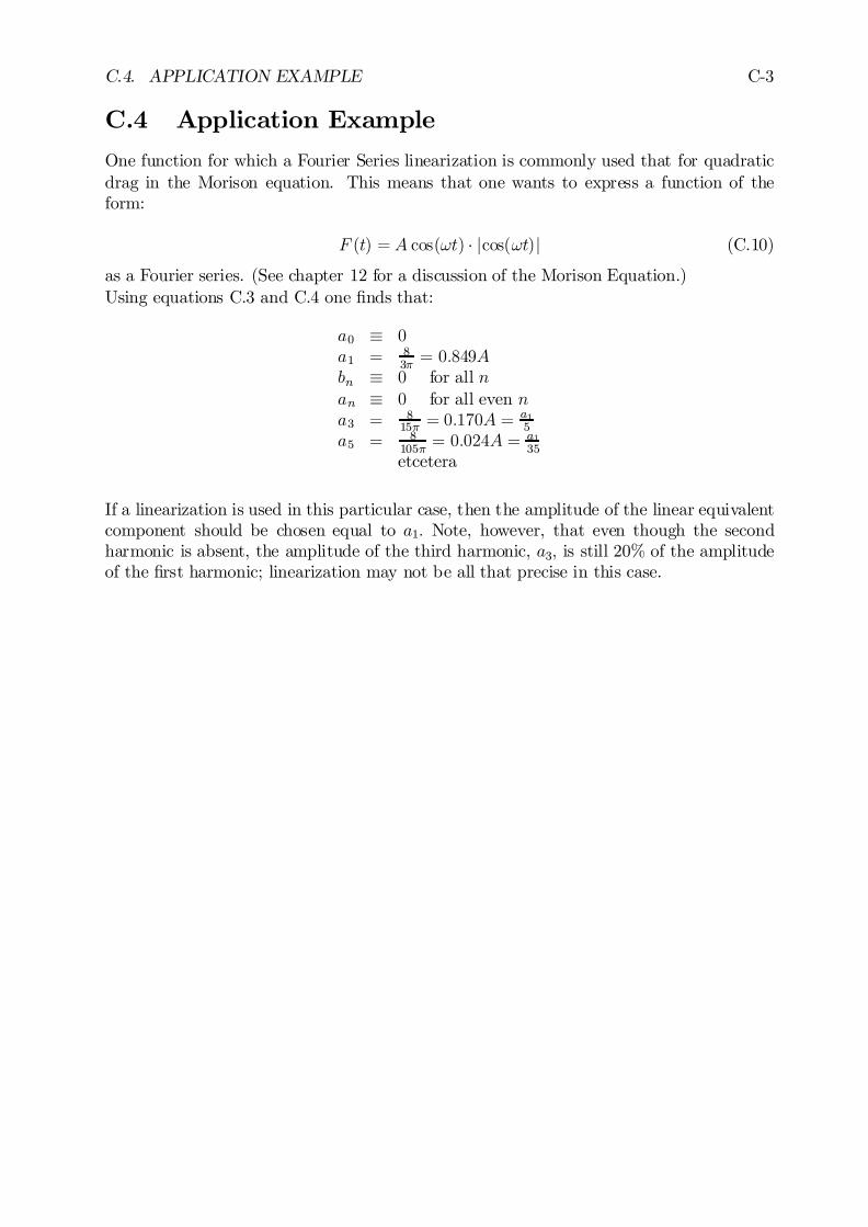
C.4. APPLICATION EXAMPLE C-3
C.4 Application Example
One function for which a Fourier Series linearization is commonly used that for quadraticdrag in the Morison equation. This means that one wants to express a function of theform:
F (t) = A cos(!t) ¢ jcos(!t)j (C.10)
as a Fourier series. (See chapter 12 for a discussion of the Morison Equation.)Using equations C.3 and C.4 one …nds that:
a0 ´ 0a1 = 8
3¼= 0:849A
bn ´ 0 for all nan ´ 0 for all even na3 = 8
15¼ = 0:170A =a15
a5 = 8105¼
= 0:024A = a135
etcetera
If a linearization is used in this particular case, then the amplitude of the linear equivalentcomponent should be chosen equal to a1: Note, however, that even though the secondharmonic is absent, the amplitude of the third harmonic, a3; is still 20% of the amplitudeof the …rst harmonic; linearization may not be all that precise in this case.

C-4 APPENDIX C. FOURIER SERIES APPROXIMATIONS
.
Bibliography
[Bales, 1983] Bales, S. L. (1983). Wind and Wave Data for Seakeeping Performance As-sessment. Technical report, Prepared for Seakeeping Committee ITTC, Athens, Greece.
[Bathe and Wilson, 1976] Bathe, K. and Wilson, E. L. (1976). Numerical Methods inFinite Element Analysis. Technical report, Prentice Hall, Englewood Cli¤s, 1976.
[Boese, 1970] Boese, P. (1970). Eine Einfache Methode zur Berechnung der Wiederstand-serhöhung eines Schi¤es in Seegang. Technical Report 258, Institüt für Schi¤bau derUniversität Hamburg, BRD.
[Bosch and Vugts, 1966] Bosch, J. J. v. d. and Vugts, J. H. (1966). Roll Damping byFree Surface Tanks. Technical Report 83-S, Netherlands Ship Research Centre TNO,Shipbuilding Department, Delft, The Netherlands.
[Bowers, 1975] Bowers, E. C. (1975). Long Period Oscillations of Moored Ships Subject toShort Wave Seas. Trans. Royal Institution of Naval Architects.
[Chislett and Bjorheden, 1966] Chislett, M. S. and Bjorheden, O. (1966). In‡uence of ShipSpeed on the E¤ectiveness of a Lateral-Thrust Unit. Technical Report Hy-8, Hydro- OgAerodynamisk Laboratorium, Lyngby, Denmark.
[Clauss, 1992] Clauss, G. (1992). O¤shore Structures, Volume 1, Conceptual Design andHydromechanics. Springer, London, UK.
[Conolly, 1974] Conolly, J. E. (1974). Standards of Good Seakeeping for Destroyers andFrigates in Head Seas. In International Symposium on the Dynamics of Marine Vehiclesand Structures in Waves, London, UK, number 8.
[Cramer and et.al., 1993] Cramer, E. and et.al. (1993). Fatigue in Side Shell Longitudinalsdue to External Wave Pressure. OMAE, II:267–272.
[Cummins, 1962] Cummins, W. E. (1962). The Impulse Response Function and Ship Mo-tions. In International Symposium on Ship Theory, Hamburg, Germany, number 8.
[Dalzell, 1976] Dalzell, J. F. (1976). Application of the Fundamental Polynomial Modelto the Added Resistance Problem. In Eleventh Symposium on Naval Hydrodynamics,London, University College, London, UK.
[Delany and Sorensen, 1970] Delany, N. K. and Sorensen, N. E. (1970). Low Speed Dragof Cylinders of Various Shapes. Technical Report 3038, NACA.
D-1

D-2 BIBLIOGRAPHY
[DetNorskeVeritas, 1989] DetNorskeVeritas (1989). Rules for the Classi…cation of FixedO¤shore Installations. Technical report, DNV, Hovik, Norway.
[Dev, 1996] Dev, A. (1996). Viscous E¤ects in Drift Forces on Semi-Submersibles. PhDthesis, Delft University of Technology, The Netherlands.
[Edwards, 1985] Edwards, R. Y. (1985). Hydrodynamic Forces on Vessels Stationed in aCurrent. In OTC 1985, Paper No. 5032, Houston, Texas, USA.
[English and Wilde, 1976] English, J. W. and Wilde, D. A. (1976). Hydrodynamic Posi-tioning. In NECIES, Presented at a Joint Meeting with RINA, December 8, 1976.
[Faltinsen, 1990] Faltinsen, O. M. (1990). Sea Loads on O¤shore Structures. Number ISBN0-521-37285-2, 1990 / ISBN 0-521-45870-6, 1993. University Press, Cambridge, UK.
[Faltinsen and Loken, 1978a] Faltinsen, O. M. and Loken, E. A. (1978a). Drift Forces andSlowly Varying Forces on Ships abd O¤shore Structures. Technical Report 1, NorwegianMaritime Research.
[Faltinsen and Loken, 1978b] Faltinsen, O. M. and Loken, E. A. (1978b). Drift Forces andSlowly Varying Horizontal Forces on a Ship in Waves. In Timman Symposium on AppliedMathematics, Delft, The Netherlands.
[Faltinsen and Loken, 1979] Faltinsen, O. M. and Loken, E. A. (1979). Slow Drift Oscilla-tions On a Ship in Irregular Waves. Journal of Applied Research, (1).
[Fang, 1985] Fang, Z. (1985). A New Method for Calculating the Fundamental PotentialFunctions Induced by a Source/Dipole Polygon. Applied Mathematics and Mechanics,6(7).
[Fossen, 1994] Fossen, T. I. (1994). Guidance and Control of Ocean Vehicles. John Wileyand Sons, Chichester, England.
[Frank, 1967] Frank, W. (1967). Oscillation of Cylinders in or below the Free Surface ofDeep Fluids. Technical Report 2375, Naval Ship Research and Development Centre,Washington DC, USA.
[Franzen, 1962] Franzen, A. (1962). Ghost from the Depths: the Warship Vasa. NationalGeographic, pages 42–57.
[Gerritsma and Beukelman, 1972] Gerritsma, J. and Beukelman, W. (1972). Analysisof the Resistance Increase in Waves of a Fast Cargo-ship. International ShipbuildingProgress, 18(217).
[Haskind, 1957] Haskind, M. (1957). The Exciting Forces and Wetting of Ships in Waves(in Russian). Izvestia Akademii Nauk SSSR, Otdelenie Tskhnicheshikh Nauk, (7):65–79.
[Herschel, 1897] Herschel, C. (1897). On the Origin of the Chezy Formula. Journal of theAssociation of Engineering Societies, 18.
[Hoerner, 1965] Hoerner, S. F. (1965). Fluid Dynamic Drag.
BIBLIOGRAPHY D-3
[Holtrop, 1977] Holtrop, J. (1977). A Statistical Analysis of Performance Results. Inter-national Shipbuilding Progress, 24.
[Holtrop, 1984] Holtrop, J. (1984). A Statistical Reanalysis of Resistance and Propulsiondata. International Shipbuilding Progress, 31.
[Holtrop and Mennen, 1982] Holtrop, J. and Mennen, G. (1982). An Approximate PowerPrediction Method. International Shipbuilding Progress, 89.
[Hooft, 1970] Hooft, J. P. (1970). Aspects of Semi-Submersible Platforms, MARIN publi-cation 400. PhD thesis, Delft University of Technology, The Netherlands.
[Hsu and Blenkarn, 1970] Hsu, F. H. and Blenkarn, K. A. (1970). Analysis of peak mooringforces caused by slow vessel drift oscillations in random seas. In O¤shore TechnologyConference, number 1159, Houston, USA.
[Huijsmans, 1996] Huijsmans, R. H. M. (1996). Motions and Drift Forces on Moored Ves-sels in Current. PhD thesis, Delft University of Technology, The Netherlands.
[Ikeda et al., 1978] Ikeda, Y., Himeno, Y., and Tanaka, N. (1978). A Prediction Methodfor Ship Rolling. Technical Report 00405, Department of Naval Architecture, Universityof Osaka Prefecture, Japan.
[Isherwood, 1973] Isherwood, M. A. (1973). Wind Resistance of Merchant Ships. Trans.Royal Institution of Naval Architects.
[Iversen and Balent, 1951] Iversen, H. W. and Balent, R. (1951). A Correlating Modulusfor the Fluid Resistance in Accelerated Motion. Journal of Applied Physics, 22(3):324–328.
[John, 1949] John, F. (1949). On the Motions of Floating Bodies, Part I. Comm. on Pureand Applied Mathematics, pages 13–57.
[Joseph, 1973] Joseph, D. D. (1973). Domain Perbutations: The Higher Order Theory ofIn…nitesimal Water Waves. Arch. Rational Mech. Anal., 51:295–303.
[Journée, 1976a] Journée, J. M. J. (1976a). Motions, Resistance and Propulsionof a Ship in Longitudinal Regular Waves. Technical Report 428, Delft Univer-sity of Technology, Ship Hydromechanics Laboratory, The Netherlands. (Internet:http://dutw189.wbmt.tudelft.nl/~johan or http://www.shipmotions.nl).
[Journée, 1976b] Journée, J. M. J. (1976b). Prediction of Speed and Behaviour of aShip in a Seaway. International Shipbuilding Progress, 23(265):285–313. (Internet:http://dutw189.wbmt.tudelft.nl/~johan or http://www.shipmotions.nl).
[Journée, 1991] Journée, J. M. J. (1991). Motions of Rectangular Barges. In Proceedings10th International Conference on O¤shore Mechanics and Arctic Engineering, Stavanger,Norway.
[Journée, 1992] Journée, J. M. J. (1992). Strip Theory Algorithms, Revised Report 1992.Technical Report 912, Delft University of Technology, Ship Hydromechanics Laboratory,The Netherlands.
D-4 BIBLIOGRAPHY
[Journée, 1997] Journée, J. M. J. (1997). Liquid Cargo and Its E¤ect onShip Motions. In STAB’97 Conference, Varna, Bulgaria. (Internet:http://dutw189.wbmt.tudelft.nl/~johan or http://www.shipmotions.nl).
[Journée, 1999] Journée, J. M. J. (1999). User Manual of SEAWAY, Release 4.18 (09-10-1999). Technical Report 1212, Delft University of Technology, Ship Hydromechan-ics Laboratory, The Netherlands. (Internet: http://dutw189.wbmt.tudelft.nl/~johan orhttp://www.shipmotions.nl).
[Journée, 2000] Journée, J. M. J. (2000). Theoretical Manual of SEAWAY (Release4.18). Technical Report 1216, Delft University of Technology, Ship HydromechanicsLaboratory, The Netherlands. (Internet: http://dutw189.wbmt.tudelft.nl/~johan orhttp://www.shipmotions.nl).
[Journée and van ’t Veer, 1995] Journée, J. M. J. and van ’t Veer, A. P. (1995). FirstOrder Wave Loads in Beam Waves. In Proceedings 5th International O¤shore and PolarEngineering Conference, The Hague. (Internet: http://dutw189.wbmt.tudelft.nl/~johanor http://www.shipmotions.nl).
[Keulegan and Carpenter, 1958] Keulegan, G. H. and Carpenter, L. H. (1958). Forces onCylinders and Plates in an Oscillating Fluid. Journal of Research of the National Bureauof Standards, 60(Research Paper 2857).
[Kim and Breslin, 1976] Kim, C. H. and Breslin, J. P. (1976). Prediction of slow driftoscillations of a moored ship in head seas. In Proceedings BOSS Conference.
[Korkut and Hebert, 1970] Korkut, M. and Hebert, E. (1970). Some Notes on Static An-chor Chain Curve. In O¤shore Technology Conference, 1970, Dallas, Texas, USA.,number OTC 1160, Dallas, Texas, USA.
[Korvin-Kroukovsky and Jacobs, 1957] Korvin-Kroukovsky, B. V. and Jacobs, W. R.(1957). Pitching and Heaving Motions of a Ship in Regular Waves. TransactionsSNAME, 65:590–632.
[Kudou, 1977] Kudou, K. (1977). The Drifting Force Acting on a Three-Dimensional Bodyin Waves. Journal of the Society of Naval Architects of Japan, 141.
[Kuiper, 1992] Kuiper, G. (1992). The Wageningen Propeller Series. Technical Report92-001, MARIN, Wageningen.
[Kuiper, 1997] Kuiper, G. (1997). Resistance and Propulsion of Ships, Lecture Notes.Technical Report 847-K, Delft University of Technology.
[Kwan, 1990] Kwan, C. T. (1990). Design Practice for Mooring of Floating Production Sys-tems. The Society of Naval Architects and Marine Engineers, O¤shore Station KeepingSymposium, Houston, Texas USA.
[Lamb, 1932] Lamb, H. (1932). Hydrodynamics. Dover Publications, Inc., New York, 6edition.
[Lewis, 1929] Lewis, F. M. (1929). The Inertia of Water Surrounding a Vibrating Ship. InTransactions SNAME.

BIBLIOGRAPHY D-5
[Lienhard, 1966] Lienhard, J. H. (1966). Synopsis of Lift, Drag, and Vortex FrequencyData for Rigid Circular Cylinders. Technical Report 300, Washington State University,College of Engineering, Research Division.
[Lloyd, 1989] Lloyd, A. R. J. M. (1989). Seakeeping, Ship Behaviour in Rough Weather.Number ISBN 0-7458-0230-3. Ellis Horwood Limited, Market Cross House, CooperStreet, Chichester, West Sussex, P019 1EB England.
[Maruo, 1960] Maruo, H. (1960). The Drift of a Body Floating in Waves. Journal of ShipResearch, 4(3).
[Massie, 1997] Massie, W. W. (1997). O¤shore Moorings. Technical Report OT-4661, DelftUniversity of Technology, Civil Engineering Department.
[McClure et al., 1990] McClure, A. C., McClure, S., and Edwards, R. (1990). Dynamic Po-sitioning Dynamics. In The Society of Naval Architects and Marine Engineers, O¤shoreStation Keeping Symposium 1990, Houston, Texas, USA, number 8.
[Minsaas et al., 1986] Minsaas, K. J., Thon, H., and Kauczynski, W. (1986). In‡uenceof Ocean Environment on Thruster Performance. In International Symposium on Pro-peller and Cavitation, Supplementary Volume, Editorial O¢ce of Shipbuilding China,Shanghai, China.
[Morison et al., 1950] Morison, J. R., O’Brien, M., Johnson, J., and Schaaf, S. (1950).The Forces Exerted by Surface Waves on Piles. In Petroleum Transactions, AIME 1950,volume 189, pages 149–157.
[Newman, 1962] Newman, J. N. (1962). The Exciting Forces on Fixed Bodies in Waves.Journal of Ship Research, 6(4):10–17.
[Newman, 1977] Newman, J. N. (1977). Marine Hydrodynamics. MIT Press, Cambridge,UK.
[Newman, 1985] Newman, J. N. (1985). Algorithms for the Free-Surface Green Function.Journal of Engineering Mathematics, 19:57–67.
[Newman, 1993] Newman, J. N. (1993). Wave-Drift Damping of Floating Bodies. Journalof Fluid Mechanics, 249:241–259.
[Ochi, 1964] Ochi, M. K. (1964). Prediction of Occurence and Severity of Ship Slammingat Sea. In Proceedings of 5th O.N.R. Symposium, Bergen, Norway.
[Ochi and Motter, 1974] Ochi, M. K. and Motter, E. (1974). Prediction of Extreme ShipResponses in Rough Seas in the North Atlantic. In Proceedings of the InternationalSymposium on the Dynamics of Marine Vehicles and Structures in Waves London, UK,Paper 20, number 20.
[OCIMF, 1977] OCIMF (1977). Prediction of Wind and Current Loads on VLCCs. InTOil Companies International Marine Forum, London, UK, 1977.
[Ogilvie, 1964] Ogilvie, T. (1964). Recent progress towards the understanding and predic-tion of ship motions. In Proc. 5th Symposium on Naval Hydrodynamics.
D-6 BIBLIOGRAPHY
[Ogilvie, 1963] Ogilvie, T. F. (1963). First and Second Order Forces on a Cylinder Sub-merged under a Free Surface. Journal of Fluid Mechanics, pages 451–472.
[Oortmerssen, 1976a] Oortmerssen, G. v. (1976a). The Motions of a Moored Ship in Waves.Journal of Ship Research, 4(3).
[Oortmerssen, 1976b] Oortmerssen, G. v. (1976b). The Motions of a Moored Ship in Waves.Technical Report 510, MARIN.
[Oortmerssen et al., 1984] Oortmerssen, G. v., van den Boom, H. J. J., and Pinkster, J. A.(1984). Mathematical Simulation of the Behaviour of Ships Moored to O¤shore Jetties.ASCE.
[Pastoor, 1997a] Pastoor, L. (1997a). Combination of Local and Global Wave InducedLoads on Side Shell Longitudinals of FPSO ’Glas Dowr’ (Master Thesis, Part II). Tech-nical report, Delft University of Technology, Ship Hydromechanics Laboratory, TheNetherlands.
[Pastoor, 1997b] Pastoor, L. (1997b). External Wave Pressure Loading of Side Shell Longi-tudinals of FPSO ’Glas Dowr’(Master Thesis, Part I). Technical report, Delft Universityof Technology, Ship Hydromechanics Laboratory, The Netherlands.
[Pinkster, 1976] Pinkster, J. A. (1976). Low-Frequency Second Order Forces on VesselsMoored at Sea. In Eleventh Symposium on Naval Hydrodynamics, London, UniversityCollege, London, UK.
[Pinkster, 1977] Pinkster, J. A. (1977). Computations of the First and Second Order WaveForces on Bodies oscillating in Regular Waves. In Second International Conference onNumerical Ship Hydrodynamics, Berkeley, USA.
[Pinkster, 1978] Pinkster, J. A. (1978). Wave feed-forward as a means to improve dynamicpositioning. In O¤shore Technology Conference, number OTC 3057, Houston, USA.
[Pinkster, 1979] Pinkster, J. A. (1979). Mean and Low Frequency Wave Drifting Forceson Floating Structures. Ocean Engineering.
[Pinkster, 1980] Pinkster, J. A. (1980). Low Frequency Second Order Wave Exciting Forceson Floating Structures. PhD thesis, Delft University of Technology, The Netherlands.
[Pinkster and Hooft, 1978] Pinkster, J. A. and Hooft, J. P. (1978). Computations of theFirst and Second Order Wave Forces on Bodies oscillating in Regular Waves. In FirstInternational Ocean Development Conference, Tokyo, Japan.
[Remery and Hermans, 1971] Remery, G. F. M. and Hermans, J. A. (1971). The slowdrift oscillations of a moored object in random seas. In O¤shore Technology Conference,number OTC 1500, Houston, USA.
[Remery and Hermans, 1972] Remery, G. F. M. and Hermans, J. A. (1972). The slowdrift oscillation of a moored object in random seas. Journal of the Society of PetroleumEngineers.
BIBLIOGRAPHY D-7
[Remery and van Oortmerssen, 1973] Remery, G. F. M. and van Oortmerssen, G. (1973).The mean wave, wind and current forces on o¤shore structures and their role in thedesign of mooring systems. In O¤shore Technology Conference, number OTC 1741,Houston, USA.
[Rijn, 1990] Rijn, L. V. (1990). Principles of Sediment Transport i98n Rivers, Estuariesand Coastal Areas. Number ISSN 90-8000356-2-9 bound, NUGI 186/831. AmsterdamAqua Publications - I11.
[Sarpkaya and Isaacson, 1981] Sarpkaya, T. and Isaacson, M. (1981). Mechanics of WaveForces on O¤shore Structures. Number ISBN 0-442-25402-4. Van Nostrand ReinholdCompany Inc., New York.
[Schlichting, 1951] Schlichting, H. (1951). Grenzschicht-Theorie. G. Braunsche Hofbuch-druckerei und Verlag, GmbH, Karlsruhe.
[Shields, 1936] Shields, A. (1936). Anwendung der aehnlichkeitsmechanik un turbulenz-forschung auf die geschiebebewegung. Mitt. Preuss Versuchanstalt fur Wasserbau undSchi¤bau, Berlin, (26).
[St. Denis and Pierson, 1953] St. Denis, M. and Pierson, W. J. (1953). On the Motion ofShips in Confused Seas. Transactions SNAME, 61:1–53.
[Suyehiro, 1924] Suyehiro, K. (1924). The Drift of Ships Caused by Rolling Among Waves.In Transactions of INA, volume 66, pages 60–76.
[Tasai, 1959] Tasai, F. (1959). On the Damping Force and Added Mass of Ships Heav-ing and Pitching. Technical report, Research Institute for Applied Mechanics, KyushuUniversity, Japan. Vol. VII, No 26.
[Tasai, 1969] Tasai, F. (1969). Improvements in the Theory of Ship Motions in Longitudi-nal Waves. In Proceedings 12th I.T.T.C.
[Tasaki, 1963] Tasaki, R. (1963). Researches on Seakeeping Qualities of Ships in Japan,Model Experiments in Waves, On the Shipment of Water in Head Waves. Journal of theSociety of Naval Architects of Japan, 8.
[Timman and Newman, 1962] Timman, R. and Newman, J. N. (1962). The CoupledDamping Coe¢cients of a Symmetric Ship. Journal of Ship Research, 5(4):1–7.
[Tuck, 1970] Tuck, E. O. (1970). Ship Motions in Shallow Water. Journal of Ship Research,14(4):317–328.
[Ursell, 1949] Ursell, F. (1949). On the Heaving Motion of a Circular Cylinder on theSurface of a Fluid. Quarterly Journal of Mechanics and Applied Mathematics, II.
[Van den Boom, 1985] Van den Boom, H. (1985). Dynamic behaviour of mooring lines. InBehaviour of O¤shore Structures, Elsevier Science Publishers, B.V., Amsterdam.
[Verhagen and van Wijngaarden, 1965] Verhagen, J. and van Wijngaarden, L. (1965).Non-linear oscillations of ‡uid in a container. Journal of Fluid Mechanics, 22(4):737–751.
D-8 BIBLIOGRAPHY
[Vugts, 1970] Vugts, J. H. (1970). The Hydrodynamic Forces and Ship Motions in Waves.PhD thesis, Delft University of Technology, The Netherlands.
[Wehausen and Laitone, 1960] Wehausen, J. V. and Laitone, E. V. (1960). Handbuch derPhysik. Springer Verlag, Berlin.
[Wheeler, 1970] Wheeler, J. D. (1970). Method for calculating forces produced by irregularwaves. Journal of Petroleum Technology.
[Wichers, 1979] Wichers, J. E. W. (1979). On the slow motions of tankers moored to singlepoint mooring systems. In Proceedings BOSS Conference, London, UK.
[Wichers, 1988] Wichers, J. E. W. (1988). A Simulation Model for a Single Point MooredTanker. PhD thesis, Delft University of Technology, The Netherlands.
[Wichers, 1992] Wichers, J. E. W. (1992). Lecture notes on ocean engineering. In IHEEDelft 1992, Part I: Introduction, number IHEE 1992, Delft.