of the status of finite element methods for partial ... · pdf filenasa contractor...
TRANSCRIPT

NASA Contractor Repdrt' 1?8222 ICASE Report No. 86-77
ICASE SURVEY OF THE STATUS OF FINITE ELEMENT METHODS FOR PARTIAL DIFFERENTIAL EQUATIONS
Roger Temam
(NASA-CH-178222) S U R V E Y OF 3EE STATUS OF N i l 7- 1 7 456 E I U ' I E EL&f'lEN'L EElECDS E C S E P 6 1 1 A L L X f E k R E l i ' L I A L E Q c A l X O N S F i n a l heI;ort ( N A S A ) t4 P C S C L 1 2 A Unclas
G3/64 44010
Contract No. NAS1-18107
November 1986
Institute for Computer Applications in Science and Engineering NASA Langley Research Center, Hampton, Virginia 23665
Operated by the Universities Space Research Association . .
National Aeronautics and Space Administration
Langley Research Canter Hampton Virginia 23665
https://ntrs.nasa.gov/search.jsp?R=19870008023 2018-05-03T12:27:30+00:00Z

SURVEY OF TBE STATUS OF FINITE ELEMENT METHODS
FOR PARTIAL DIF’FERENITAL EQUATIONS
Roger T e m a m
L a b o r a t o i r e d’hnalyse Numerique
Univers i te ’ P a r i s Sud, 91405 Orsay, France
ABSTRACT
The f i n i t e element methods (FEM) have proved t o be a powerful t echn ique
f o r t h e s o l u t i o n of boundary va lue problems a s s o c i a t e d wi th p a r t i a l
d i f f e r e n t i a l equa t ions of e i t h e r e l l i p t i c , p a r a b o l i c , o r hype rbo l i c type.
They a l s o have a good p o t e n t i a l f o r u t i l i z a t i o n on p a r a l l e l computers
p a r t i c u l a r l y i n r e l a t i o n t o the concept of domain decomposi t ion.
Th i s r e p o r t i s in tended as an i n t r o d u c t i o n t o t h e FEM f o r t h e
n o n s p e c i a l i s t . It c o n t a i n s a survey which i s t o t a l l y nonexhaus t ive , and i t
a l s o c o n t a i n s as an i l l u s t r a t i o n , a r e p o r t on some new r e s u l t s concern ing two
s p e c i f i c a p p l i c a t i o n s , namely a free boundary f l u i d - s t r u c t u r e i n t e r a c t i o n
problem and t h e Eu le r e q u a t i o n s f o r i n v i s c i d f lows.
I T h i s work was suppor ted under the N a t i o n a l Aeronaut ics and Space \ Admin i s t r a t ion under NASA Con t rac t No. NAS1-18107 whi l e t h e a u t h o r w a s I n
r e s i d e n c e a t t h e I n s t i t u t e f o r Computer App l i ca t ions i n Sc ience and Engineer ing (LCASE) , Hampton, VA 23665-5225.
i

INTRODUCTION
It is t o t a l l y imposs ib le t o survey the theory of f i n i t e element methods
w i t h i n a few pages, and t h e o b j e c t of t h i s a r t i c l e is t o d e s c r i b e f o r t h e
n o n s p e c i a l i s t some very b a s i c ideas and c o n c e p t s i n f i n i t e elements approxima-
t i o n s and t o d i s c u s s some f u t u r e t r e n d s i n t h e theory without any a t tempt a t
be ing exhaus t ive . Beside t h i s survey p a r t , t h i s ar t ic le con ta ins i n S e c t i o n s
8 and 9 a r e p o r t on some new r e s u l t s concerning two s p e c i f i c problems, v i z . - a
and t h e Euler equa t ions f o r
i n v i s c i d flows.
There i s no agreement about t h e f i r s t appearance of t h e method. F i n i t e
element methods have probably been used f o r many yea r s f o r computing and
eng inee r ing purposes i n a more o r less e x p l i c i t form. R. Courant mentions i n
[ l o ] t h e approximation of a funct-Lon i n by continuous p iecewise l i n e a r
f u n c t i o n s on a t r i a n g u l a t i o n , and t h i s may be t h e f i r s t appearance i n t h e
mathematical l i t e r a t u r e .
Although i t is d i f f i c u l t t o t r a c k t h e f i r s t appearance of t h e method,
t h e r e is no doubt t h a t t h e f i r s t sys t ema t i c and large scale u t i l i z a t i o n s of
t h e f i n i t e element methods (FEM) occurred i n t h e s i x t i e s i n s o l i d mechanics
engineer ing . The per iod co inc ides of course wi th t h e f i r s t computers and t h e
e a r l y stages of what we now ca l l s c i e n t i f i c computing. Probably t h e reasons
which made FEM immediately popular among s o l i d mechanics eng inee r s is t h a t , as
w e recall below, t h e foundat ions of the FEM co inc ide wi th some very funda-
mental concepts i n s o l i d mechanics. The method has then spread wi th d i f f e r e n t
l e v e l s of response i n f l u i d mechanics, op t imiza t ion and c o n t r o l t heo ry , and
among mathematicians.

-2-
Alike t h e s o l i d mechanis ts , mathematicians (numerical a n a l y s t s and some
more t h e o r e t i c a l l y o r i e n t e d mathematicians) have been working i n FEM because
t h e methods are a p p r o p r i a t e f o r mathematical t rea tment and are very close i n
t h e i r fundamental concepts t o t h e i d e a s and t o o l s which are used i n t h e
mathematical t reatment of t h e l i n e a r and nonl inear boundary v a l u e problems by
f u n c t i o n a l a n a l y s i s .
The mathematical and engineer lng l i t e r a t u r e on FEM f o r p a r t i a l
d i f f e r e n t i a l equat ions i s abundant, and t h e r e i s no way t o survey i t here .
The ques t ions t h a t w e address are t h e fol lowing ones: I n S e c t i o n 1 , w e recall
t h e p r i n c i p l e of weak formula t ions , and i n S e c t i o n 2 , w e recall t h e r o l e of
domain decomposition i n t h e contex t of s t r u c t u r a l mechanics. We r e t u r n t o
domain decomposition i n S e c t i o n 9 as it relates t o f u t u r e developments i n t h e
FEM i n r e l a t i o n with p a r a l l e l computation and some p o s s i b l e e x t e n s i o n s of t h e
method. S e c t i o n s 3 t o 5 are devoted t o t h e d e s c r i p t i o n of very t y p i c a l
mathematical r e s u l t s . S e c t i o n 3 d e s c r i b e s t h e g e n e r a l mathematical framework
and t h e mos t common f i n i t e elements. S e c t i o n 4 provides some convergence and
error results whi le S e c t i o n 5 i s an i n t r o d u c t i o n t o mixed and hybr id f i n i t e
e lements . Some s p e c i f i c a p p l i c a t i o n s (among many o t h e r s ) of t h e FEM are t h e n
descr ibed . S e c t i o n 6 is r e l a t e d t o t h e Navier-Stokes equat ions . S e c t i o n 7
d e a l s with f l u i d - s t r u c t u r e i n t e r a c t i o n s problems, and S e c t i o n 8 d e a l s wi th t h e
a p p l i c a t i o n s of FEM to t h e s o l u t i o n of t h e E u l e r equat ions. F i n a l l y , as
i n d i c a t e d above, w e r e t u r n i n S e c t i o n 9 t o domain decomposition and t h e r o l e
t h a t t h i s can p lay in f u t u r e developments f o r FEM.

-3-
FOUNDATIONS OF "€?E FEM
The f i n i t e element methods l i e on two fundamental i d e a s :
- t h e weak fo rmula t ion of a boundary value problem,
- t h e domain decomposition, i.e., t h e decomposition of t h e domain
cor responding t o t h e problem i n t o smaller subdomains, t h e elements.
A s mentioned above, both i d e a s a r e c l o s e l y r e l a t e d t o b a s i c concepts of
s o l i d mechanics. The weak formula t ion of a boundary va lue problem co inc ides
wi th t h e v i r t u a l work theorems and energy p r i n c i p l e s in t h e s ta t ics of
s o l i d s . Domain decomposition is a l s o a n e x t r a p o l a t i o n of t he n a t u r a l approach
i n s t r u c t u r a l mechanics where l a r g e s t r u c t u r e s c o n s i s t of smaller subs t ruc -
t u r e s which are p rope r ly connected o r assembled, and the s tudy of t he l a r g e
s t r u c t u r e i s reduced t o t h a t of t he e lementary s t r u c t u r e s and t h e i r
connec t ions .
1. Weak Formulations
We begin by r e c a l l i n g b r i e f l y the weak fo rmula t ion of some boundary va lue
problems i n s o l i d and f l u i d mechanics. Other examples of weak fo rmula t ions
w i l l appear below ( a b s t r a c t boundary value problems).
1 .a. Weak Formulations i n So l id Mechanics
Consider a s o l i d body which f i l l s a t rest a r eg ion Q of I€? w i t h
boundary r . We assume t h a t t h e body is sub jec t ed t o volumic f o r c e s of
d e n s i t y f = ( f l , f 2 , f 3 ) i n R and t o s u r f a c e ( t r a c t i o n ) f o r c e s of s u r f a c e
d e n s i t y F = (F1,F2,F3) on some par t r l of r and r eaches a r,ew
e q u i l i b r i u m p o s i t i o n . The unknowns of t h e problem are:
- t h e f i e l d d isp lacements , u = (u1 ,u2 ,u3) , u (x) xEQ, r e p r e s e n t i n g t h e

-4 -
displacement between t h e p o s i t i o n a t rest of a par t ic le XEQ and i t s
new equi l ibr ium p o s i t i o n x + u(x) .
- t h e boundary stress t e n s o r f i e l d , Q = (Uij).
Under t h e assumption of small d i sp lacements , t h e e q u i l i b r i u m e q u a t i o n s
read
bT- i j + f i = O i n 0
3
3 aa
j=l j
1 u i j v j = Fi j =1
where v = (vl ,v2,v3) is t h e u n i t outward normal on r . Usually t h e displacement u i s g iven on t h e complementary p a r t
rO of
u = U on ro.
The so-cal led set of s t a t i c a l l y a d m i s s i b l e stress t e n s o r s Sad(f ,F) i s
t h e set of t e n s o r f i e l d s u s a t i s f y i n g (1.1) and (1.2). The se t Cad(U)
i s t h e set of k i n e m a t t c a l l y admiss ib le displacement f i e l d s , i .e., t h e set of
u O s s a t i s f y i n g (1.3).
The equat ions (1.1) - (1.3) which hold f o r any material are supplemented
by t h e c o n s t i t u t i v e e q u a t i o n s of t h e material which depend on t h e material and
connect stresses and displacements . Without d e s c r i b i n g t h e s e r e l a t i o n s , w e
can already see t h e weak formula t ion of t h e problem. L e t u , u be s o l u t i o n
of (1.1) - (1.3) and l e t v be another k i n e m a t i c a l l y admiss ib le f i e l d of d i s -
placements, vcc (U) (and w = v - U E C , ~ 0 z Cad(0)). We m u l t i p l y (1.1) by ad

-5-
t h e s i m p l e s t case of l i n e a r e l a s t i c i t y we have pointwise
I wi, add t h e s e r e l a t i o n s f o r i = 1 ,2 ,3 , i n t e g r a t e over Q, and use Green
i formula and (1.2) (1.3). We o b t a i n
0 (w)dx = I fiwidx + I F w d r , f o r a l l wecad, i i 'ij 'ij n (1 - 4 )
n
where t h e E i n s t e i n summation convent ion has been used and
is t h e s t r a i n t e n s o r
E(W) = (Eij(w))
awi a w
i j 2 axj axi E: (w) = - 1 (- + -). j
I where t h e c o e f f i c i e n t s
A i n t h e space of symmetric t e n s o r s of order two. Whence (1.4) becomes
Aijkl d e f i n e a l i n e a r p o s i t i v e i n v e r t i b l e o p e r a t o r I
I n l i n e a r and n o n l i n e a r e l a s t i c i t y , the weak formula t ion (1.4) (or (1.6))
c o i n c i d e s wi th t h e r e l a t i o n given by the v i r t u a l work theorem. It l e a d s also
t o energy p r i n c i p l e s . 1 I 'A similar formula t ion is a v a i l a b l e for t h e stresses 0 . 1

-6-
1 .b. Weak Formulations i n F lu id Mechanics
Weak formula t ions i n f l u i d mechanics do not have a phys ica l i n t e r p r e t a -
t i o n as n a t u r a l as i n s o l i d mechanics. They have been in t roduced by J. Leray
( [ 1 6 ] , [17 ] , 1181) f o r t h e s tudy of weak ( i . e . , nonregular ) s o l u t i o n s of t h e
Navier-Stokes equa t ions i n an a t tempt t o e x p l a i n tu rbu lence by t h e appearance
of s i n g u l a r i t i e s i n t h e c u r l vec to r of t h e flow. Although we do not know y e t
i f such s i n g u l a r i t i e s ar ise i n space dimension t h r e e , t h e r e is no doubt t h a t
t h e c o n t r i b u t i o n of J. Leray has been a fundamental s t e p f o r t h e mathematical
t r ea tmen t O E the Navier-Stokes equa t ions by t h e modern methods of f u n c t i o n a l
a n a l y s i s and a l s o €o r t h e numerical t r ea tmen t of t h e equa t ions i n Computa-
t i o n a l F lu id Dynamics.
Consider f o r example t h e Navier-Stokes equa t ions of an incompress ib le
f l u i d i n the s t a t i o n a r y case. The f l u i d f i l l s a bounded r eg ion $2 of E?
wi th boundary r . I n t h e Eu le r i an r e p r e s e n t a t i o n of t h e flow, t h e unknowns
are t h e v e l o c i t y f i e l d
xECl is the v e l o c i t y of t h e par t ic le of f l u i d a t x, and p (x ) i s t h e
pressure a t po in t x. We have t h e equa t ions
u = (u1,u2,u3) and t h e p r e s s u r e f i e l d p; u = u ( x ) ,
(1.7) U A U + (u*V)u + Vp = f i n $2
(1.8) d i v u = 0 i n Cl,
where v > 0 is t h e k inemat ic v i s c o s i t y and f r e p r e s e n t s volumic
f o r c e s . Equation (1.7) i s t h e equa t ion of conse rva t ion of momentum. Equation
(1.8) is the i n c o m p r e s s i b i l i t y equa t ion , i .e., t h e equa t ion of mass conserva-
t i o n . I f r i s m a t e r i a l i z e d and moving wi th v e l o c i t y U , then t h e nons l ip

-7-
c o n d i t i o n on r i s
u = u on r .
L e t V(U) be t h e space of func t ions s a t i s f y i n g ( 1 . 8 ) and ( 1 . 9 ) . Then
ucV(U) and i f v i s a tes t f u n c t i o n i n V ( U ) , w = v - u E V ( 0 ) . We t a k e t h e
scalar product of ( 1 . 7 ) wi th w (poin twise i n $1, i n t e g r a t e over $2, and
use Green's formula. We have
grad powdx = pwovdr -I p d i v wdx = 0. n r n
Whence p d i sappea r s and w e o b t a i n t h e weak formula t ion of ( 1 . 7 ) - ( 1 . 9 ) :
( 1 . 1 0 )
UE NU) and f o r eve ry WE v(0)
3 3 a U d x + "iT j w.dx J =
i , j = l Q J J i , j = l n
3 =I j f w d x . i i i= 1
It is equ iva len t t o s a y t h a t u satisfies ( 1 . 1 0 ) o r t h a t u s a t i s f i e s ( 1 . 7 )
- ( 1 . 9 ) . The s t r i k i n g f a c t i n formulation ( 1 . 1 0 ) i s t h a t t h e p r e s s u r e
d i sappea r s and we are l e f t wi th an equat ion invo lv ing u only. Once u i s
found we know from mathematical r e s u l t s t h a t t h e r e e x i s t s p which is de f ined
up t o a n a d d i t i v e cons t an t by ( 1 . 7 ) . However, i n t h e p r a c t i c e of numerical

-8-
computations p is obta ined d i f f e r e n t l y , i n g e n e r a l , as t h e Lagrange mul t i -
p l i e r of t h e c o n s t r a i n t d i v u = 0 ( s e e S e c t i o n 5 below).
2. Domain Decomposition
I n s t r u c t u r a l mechanics i t is n a t u r a l t o compute a complicated s t r u c t u r e
by cons ider ing t h e smaller s u b s t r u c t u r e s of which i t is made. Each subs t ruc -
t u r e i s w e l l modeled, i t s behavior is w e l l unders tood , and then t h e mechanical
eng inee r s model t h e i n t e r a c t i o n ( c o n t a c t laws, etc.) of t h e d i f f e r e n t
components t o o b t a i n t h e d e s c r i p t i o n of t h e f u l l s t r u c t u r e .
A s mentioned be fo re , f i n i t e elements i n s o l i d mechanics have s t a r t e d as
an e x t r a p o l a t i o n of t h i s i d e a t o continuous bodies: t h e f u l l s o l i d body i s
decomposed i n t o smaller e lements ; a s i m p l i f i e d c o n s t i t u t i v e l a w is adopted on
each element; and a s i m p l i f i e d v e r s i o n of t h e c o n s t i t u t i v e l a w l e a d s t o
s i m p l i f i e d i n t e r a c t i o n s laws between t h e contiguous elements.
F igure 2.1

-9-
S i m i l a r l y , t h e p a r t i c l e and cells methods i n f l u i d mechanics which are
very c l o s e t o t h e f i n i t e element methods a re based on a s i m p l i f i e d a n a l y s i s of
t h e flow i n small ce l l s wi th s i m p l i f i e d f l u i d t r a n s f e r laws. The g e n e r a l i z a -
t i o n and mathematization of t h e FEM have l e d t o a more sys t ema t i c view and a
more s y s t e m a t i c approach.
Beside d i s c r e t i z a t i o n , t h e r e are s e v e r a l o t h e r good reasons t o decompose
a large domain i n t o smaller subdomains. These reasons are a l s o a t t h e h e a r t
of f u t u r e developments i n s c i e n t i f i c computation and probably f i n i t e
elements. We w i l l r e t u r n on t h i s important q u e s t i o n i n S e c t i o n 8.
WIN METHODS - M I N MATBEMATICAL RESULTS
We g i v e an overview of some t y p i c a l f i n i t e element methods and some
t y p i c a l mathematical r e s u l t s which have been obta ined .
3 . The Usual F i n i t e Elements Methods
3.a. A Model Problem
We cons ide r as a model problem t h e following mathematical problem.
We denote by 52 an open bounded domain of 'Iff, with boundary l", and
w e cons ide r a Laplace equa t ion ,
(3.1) -Au + u = f i n Q ,
wi th a s s o c i a t e d boundary cond i t ions of D i r i c h l e t and Neuman type

-10-
(3.3) - - a u - o on r l av
where r o , r l is a p a r t i t i o n of r . In t h e two-limit cases
ro = r , r l = p)
Neuman problems; t h e g e n e r a l case i s a mixed boundary va lue problem.
and r o = 0, r l = r w e o b t a i n r e s p e c t i v e l y t h e D i r i c h l e t and
L e t V be t h e space of f u n c t i o n s u s a t i s f y i n g (3.2) and posses s ing a
c e r t a i n l e v e l of r e g u l a r i t y which we do not s p e c i f y a t t he moment. The s o h -
t i o n u of (3.1) - (3.3) belongs t o V and if v is a test f u n c t i o n i n V,
w e mul t ip ly (3.1) by v, i n t e g r a t e over R , and apply Green’s formula.
Thanks t o (3.3) (and v = 0 on ro) we f i n d
( 3 . 4 )
and t h u s
(3.5)
where
( 3 -6)
and
n -I A U vdx = 1 I - a u 2 dx ax ax, n i= l n i
f o r a l l VEV
n a u a v dx + I uvdx 52
a ( u , v ) = i = l R

(3.7)
-1 1-
( f ,v) = I f ( x ) v(x)dx n
is t h e s c a l a r product i n L2(S2).
Conversely, i t can be proved (under s u i t a b l e r e g u l a r i t y assumptions) t h a t
i f u s a t i s f i e s (3.5) then u is t h e s o l u t i o n of (3.1) - (3.3). Equat ion
(3.1) i s de r ived from (3.5) by appropr i a t e methods us ing d i s t r i b u t i o n der iva-
t i v e s ; (3.2) fo l lows from "uEV" whereas (3.3) is a boundary c o n d i t i o n h idden
i n (3.5). This is a g e n e r a l f a c t w i t h weak formula t ions l i k e (3.5): some
boundary cond i t ions of t h e problem are conta ined i n t h e d e f i n i t i o n of t h e
space V , and some boundary cond i f ions a re conta ined i n t h e equa t ion (3.5).
L e t u s g i v e a more p r e c i s e d e f i n i t i o n of t h e space V. Roughly speaking ,
t h e space V w i l l be t h e space of a l l func t ions u vanish ing on and
such t h a t a ( u , u ) < QD. More p r e c i s e l y i t is easy t o see t h a t t h e e x p r e s s i o n
ro -
i s a norm on t h e space of cont inuous ly d i f f e r e n t i a b l e func t ions on which
van i sh on ro . We d e f i n e V as t h e completion of t h i s space f o r t h i s norm;
we o b t a i n t h e space
TZ
V = {vEH 1 (SZ), V I = 0 ) rO
where H1(Q) i s t h e Sobolev space
(3.9)
-12-
More gene ra l ly Hm(s2), t h e Sobolev space of o r d e r m, is t h e space of
f u n c t i o n s u squa re i n t e g r a b l e i n Si ( u ~ L * ( a ) ) such t h a t a l l d e r i v a t i v e s
of o r d e r - < m are squa re i n t e g r a b l e a l s o .
3.b. Abs t rac t Boundary Value Problem
The s i t u a t i o n i n (3.5) i s t y p i c a l OE many l i n e a r e l l i p t i c boundary va lue
problems. The a b s t r a c t s e t t i n g is t h e fo l lowing one:
V (norm ll*llv) - W e a r e g iven a H i l b e r t space
on V x V which is cont inuous , i .e.,
and a b i l i n e a r form a
(3.10) There e x i s t s M < such t h a t
a ( u , v ) - < M llullv nvll f o r a l l u,vEV V ’
and coerc ive , i.e.,
(3.11) There e x i s t s a > 0 such t h a t
a ( u , u ) - > a IIullv2, f o r a l l UEV.
- We a r e given a l s o a l i n e a r continuous form 2 on V , i.e., an element
of the d u a l V’ o€ V
and t h e n the problem is
To f i n d uEV such t h a t
a ( u , v ) = < t , v > , f o r a l l VEV.
(3.12)

-1 3-
Desp i t e i t s s i m p l i c i t y , (3.12) is a p p l i c a b l e t o many i n t e r e s t i n g boundary
va lue problems i n mechanics and physics. The e x i s t e n c e and uniqueness of a
s o l u t i o n u of (3.12) is c l a s s i c a l l y provided by t h e Lax-Milgram Theorem (see
f o r i n s t a n c e [ 2 8 ] ) .
More g e n e r a l l y non l inea r e l l i p t i c boundary va lue problems can be set i n a
form similar t o (3.12) i f we a l low V t o be a Banach space and a t o be
n o n l i n e a r wi th respect t o i t s f i r s t argument (F.e., a maps V x V i n t o Wand
is l i n e a r with r e s p e c t t o its second argument). For i n s t a n c e , i t fo l lows
r e a d i l y from (1.10) t h a t t h e s t a t i o n a r y Navier-Stokes equa t ions (1.7) - (1.9)
w i th U = 0 can be w r i t t e n i n t h i s form. S i m i l a r l y , cons ide r t h e problem
(3.1) - (3.3) and r e p l a c e t h e l i n e a r equat ion
-Au + u = f i n 52
by t h e non l inea r one
(3.13)
where p i s a polynomial of odd degree wi th a p o s i t i v e l ead ing c o e € f i c i e n t .
Then (3.13), (3.2), and (3.3) can be set i n a form similar t o (3.12)
where a is t h e degree of t h e polynomial p (see [28]).

-14-
In the non l inea r case, t h e r e are no g e n e r a l assumptions on a cove r ing
a l l t h e i n t e r e s t i n g s i t u a t i o n s , and w e w i l l res t r ic t ou r se lves t o s p e c i f i c
examples.
3.c. General Form of F i n i t e Element Approximations
The d i s c r e t i z a t i o n of t h e a b s t r a c t boundary va lue problem (3.12) c o n s i s t s
i n choosing
- a family (vh)hcH of f i n i t e dimensional approximations of V
- a (au(uh, Vh))hEH of b i l i n e a r forms on vh x vh which
approximat e a.
Roughly speaking t h e r e are two types of d i s c r e t i z a t i o n s produced by t h e
f i n i t e elements:
- t h e conforming f i n i t e elements i n which t h e vh are subspaces of V of
h ighe r and h i g h e r dimensions as t h e parameter b o ,
- t h e nonconforming f i n i t e elements i n which the
of v. vh are not subspaces
Of course f i n i t e elements have been only used i n space dimension n = 2
and a t a l e s s developed s t a g e when n = 3. We cons ide r f i r s t t h e case where
Sl i s a polygonal se t . A b a s i c i n g r e d i e n t of FEM is a t r i a n g u l a t i o n of
Sl. By t h i s , w e mean a s u i t a b l e cover ing of Q by e i t h e r
- a family of t r i a n g l e s ,
- a family of r e c t a n g l e s whose s i d e s are p a r a l l e l t o t h e axes ( o r more
gene ra l q u a d r i l a t e r a l s e t s ) ,
- o r a combination of t r i a n g l e s and r e c t a n g l e s (or q u a d r i l a t e r a l sets).
The t r i a n g l e s o r r e c t a n g l e s are t h e ( f i n i t e ) "elements." The space vh
c o n s i s t s of f u n c t i o n s of a g iven type ( u s u a l l y a polynomial) on each element
-1 5-
which are p rope r ly connected. The values of t h e f u n c t i o n s of vh o r t h e i r
d e r i v a t i v e s a t some p a r t i c u l a r po in t s of t h e e l e m e n t s ( v e r t i c e s , mid-
edges,.. .) are t h e nodal va lues which f u l l y determine t h e f u n c t i o n s i n A
n a t u r a l b a s i s of vh c o n s i s t s o f t h e so-called shape func t ions : These are
t h e f u n c t i o n s of vh whose nodal va lues are 1 f o r one of them and 0 f o r
a l l t h e o t h e r s . I n most cases these f u n c t i o n s have a "small" suppor t , and
t h i s l e a d s t o f a i r l y sparse ma t r i ces €or t h e d i s c r e t i z e d problem. When a
f u n c t i o n v is def ined on Sl ( o r on an element K ) , i t s i n t e r p o l a n t on
SZ ( o r K) denoted rhv ( o r rKv) i s the f u n c t i o n of vh ( o r t h e elementary
f u n c t i o n on K) which has t h e same nodal va lues as v.
vh'
3.d. Conforming F i n i t e Elements ( n = 2) .
For second o r d e r e l l i p t i c boundary va lue problems, t h e b a s i c space V
o r a product of such spaces o r a subspace of such spaces.
The s i m p l e s t and most common elements used i n t h i s case are t h e PI
elements on t r i a n g l e s and t h e Q1 elements on r e c t a n g l e s . P1 ( r e s p e c t i v e l y
Pn) i s t h e set of polynomials of degree < 1 ( r e s p . < m ) , whereas Q 1 ( r e s p .
Qm) i s t h e set of polynomials of degree wi th respect t o each
v a r i a b l e .
is H1(Q)
- - < 1 ( r e s p . < m) - -
Some o t h e r t y p i c a l elements used fo r second o r d e r boundary va lue problems
are dep ic t ed in Figure 3.1. We w i l l r e t u r n t o t h e P1 and Q1 elements
a f t e r we b r i e f l y d e s c r i b e t h e elements i n F igu re 3.1.
T r i a n g l e s
l i n e a r : polynomials of degree < 1 on t h e t r i a n g l e s , nodal va lues = - va lues a t v e r t i c e s .

-1 6-
D Linear, quadratic, cubic triangles
e2 t ' el
I - el
TAnear, quadratic, cubic rectangles
Conforming Reduced Cubic
Hermite elements Triangle
Reduced quadratic
Triangle
Figure 3.1: Conforming Finite Elements (n = 2)

-17-
polynomials of degree < 2 on the t r i a n g l e s ; nodal va lues =
va lues a t v e r t ices and midedges.
q u a d r a t i c : -
c u b i c : polynomials of degree - < 3 on t r i a n g l e s ; nodal va lues =
va lues a t v e r t i c e s , barycenter and 1/3 p o i n t s on edges.
reduced cubic: polynomials of degree - < 3 , vanish ing a t t h e ba rycen te r on
each t r i a n g l e ; nodal va lues = values a t v e r t i c e s and 1/3
p o i n t s on edges.
Rec tangles
l i n e a r :
q u a d r a t i c :
cubic :
polynomials of degree < 1 i n each v a r i a b l e o n
r e c t a n g l e s ; nodal va lues = va lues a t v e r t i c e s .
-
polynomials of degree - < 2 i n each v a r i a b l e ; nodal
v a l u e s = va lues a t vertices, midedges, and c e n t e r .
polynomials of degree - < 3 i n each v a r i a b l e ; nodal
va lues = va lues of f u n c t i o n a t 16 d i f f e r e n t p o i n t s (see
F igure 3 . 1 ) .
reduced q u a d r a t i c : polynomials of degree - < 2 i n each v a r i a b l e s a t i s f y i n g a
l inear r e l a t i o n (on each r e c t a n g l e ) ; nodal v a l u e s =
va lues of func t ion a t v e r t i c e s and midedges.
-18-
All func t ions obta ined by t h e s e elements are g l o b a l l y Co (cont inuous)
except the q u a d r a t i c Hermite t r i a n g l e which produces C1 approximants
(cont inuous ly d i f f e r e n t i a b l e f u n c t i o n s ) .
More s p e c i a l e lements can be found i n t h e l i t e r a t u r e ; c f . f o r i n s t a n c e
t h e book of P. G. Ciarlet [ 9 ] on t h e mathematical s i d e , and t h e book of
Zienkiewicz [ 3 3 ] , t h e work of Argyris [ l ] and o t h e r s on t h e engineer ing or
mechanical s i d e s .
The more s o p h i s t l c a t e d elements produce b e t t e r (more precise) r e s u l t s but
need more computing t i m e and a good e x p e r t i s e i n f i n i t e e lements technology.
I n a nonspecial ized i n d u s t r i a l environment, t h e tendency seems t o be t h e
u t i l i z a t i o n of s imple elements of degree one o r a t most two wi th a s u i t a b l e
ref inement of t h e mesh.
As mentioned above t h e s i m p l e s t and most commonly used elements are t h e
P1 elements on t r i a n g l e s and t h e Q1 elements on r e c t a n g l e s wi th s i d e s
p a r a l l e l t o t h e x and y axes. L e t u s mention a l s o t h e q u a d r i l a t e r a l
e lements descr ibed h e r e a f t e r . A
L e t K denote t h e square ( 0 , l ) x ( 0 , l ) i n t h e 5 , TI plane.
observe t h a t a mapping F w i t h Q1 components
A
can map K on any a r b i t r a r y q u a d r i l a t e r a l K of t h e x , y plane.
image by F of a l i n e i n t h e 5 , n plane is g e n e r a l l y a curved l i n e of
We
The
t h e
x , y plane. However t h e l i n e s x = c o n s t a n t , y = c o n s t a n t , and i n p a r t i c u l a r
t h e boundary of K are mapped by F onto s t r a i g h t l i n e s of t h e x , y
plane. A n a t u r a l element on t h e q u a d r i l a t e r a l K i s t h e image by F-l of
..a

-1 9-
Figure 3.2
n
element on K:
I n g e n e r a l t h e s e elements a r e not polynomials on K. They are, however,
easy t o use and t h e i r e x p l i c i t express ion is r a r e l y used.
3.e. Conforming F i n i t e Elements (n = 3)
The t r i a n g u l a t i o n is now t h e covering of Q (= a polygonal set) by
e i t h e r t e t r a h e d r o n s o r 3-D r e c t a n g l e s whose edges are para l le l t o t h e axes o r
combinations of those.
The most common e lements are t h e
- l i n e a r , q u a d r a t i c , and cub ic te t rahedrons .
- l i n e a r , q u a d r a t i c , and cub ic 3-0 r ec t ang le s .
The d e f i n i t i o n s of t h e s e elements are the same as above i n t h e two-dimensional
case r e p l a c i n g t r i a n g l e by t e t r a h e d r o n and r e c t a n g l e by 3-D r ec t ang le . For

-20-
Linear, quadratic, cubic tetrahedrons
e 3 t
Linear, quadratic, cubic rectangles
Figure 3.3: Conforming Finite Elements (n = 3)

-21-
t h e cub ic ( t e t r a h e d r o n and 3-D r ec t ang le ) e lements , t h e nodal va lues are shown
on Figure 3 . 3 . A l l t h e s e elements lead t o f u n c t i o n s which are g l o b a l l y Co
( con t inuous ) but not more.
3 . f . Nonconforming F i n i t e Elements
A s i n d i c a t e d above, nonconforming f i n i t e elements produce approximate
which are not subspaces of V. For i n s t a n c e , the f u n c t i o n spaces
l i n e a r nonconforming t r i a n g l e descr ibed below produces, when a p p l i e d t o
Problem ( 3 . 1 2 ) , approximate f u n c t i o n s which are h igh ly d iscont inuous . S t i l l ,
i t may be u s e f u l t o u s e such elements i n a t least two cases:
'h
- F l u i d flow problems where, due t o t h e i n c o m p r e s s i b i l i t y c o n d i t i o n d ivu
= 0, t h e l i n e a r t r i a n g l e elements cannot be used i n a s t r a i g h t f o r w a r d
manner.
- Higher o r d e r problems, l i k e the biharmonic problem where most elements
desc r ibed above f a i l t o produce f u n c t i o n s , and thus t h e approximate Ci
z spaces Vh would not be included i n H (Q) (= t h e n a t u r a l space f o r a
biharmonic problem).
Nonconforming l i n e a r elements
2-D Case ( T r i a n g l e s )
Polynomials of degree - < 1 on t h e t r - a n g l e s
Nodal va lues = v a l u e s a t midedges

-22-
3-D Case (Tet rahedron)
Polynoms of degree < 1 on t h e t e t r a h e d r o n s
Nodal va lues = va lues a t ba rycen te r of f a c e s
-
The g loba l f u n c t i o n s are t o t a l l y d i scon t inuous w i t h d i s c o n t i n u i t i e s along
t h e edges of t r i a n g l e s ( o r f a c e s of t e t r a h e d r o n s ) except f o r t h e b a r y c e n t e r s
(of edges o r f aces ) . The method is n e v e r t h e l e s s convergent and e f f i c i e n t ,
p a r t i c u l a r l y f o r f l u i d flows: see t h e book of F. Thomasset [32] which is
f u l l y devoted t o t h e u t i l i z a t i o n of t h e s e e l e m e n t s i n 2-D flows.
3.g. Curved boundar ies
Curved boundaries can be approximated by polygonal l i n e s . A l t e r n a t i v e l y
one can use t h e so -ca l l ed i sopa rame t r i c elements: t h e element is t h e image by
a n appropr i a t e ( s imple ) mapping of a t r i a n g l e o r a r e c t a n g l e and the f u n c t i o n
reduces on t h e element t o t h e composition of a polynomial w i th t h a t mapping.
A similar s i t u a t i o n occurred wi th the Q1 q u a d r i l a t e r a l elements.
4. Convergence and E r r o r Es t imate
Concerning convergence and e r r o r estimates t h e s i t u a t i o n is d i f f e r e n t f o r
l i n e a r and non l inea r problems.
4.a. Linear Problems
Two t y p e of r e s u l t s have been der ived i n r e l a t i o n wi th e r r o r computation
and convergence ( s e e € o r i n s t a n c e P. G. Ciar le t [91):
- i n t e r p o l a t i o n e r r o r ,
- approximation e r r o r .
-23-
When vh is a conforming f i n i t e element space and u i s a f u n c t i o n i n V (o r
u s u a l l y i n a smaller space) , w e consider t h e i n t e r p o l a n t rhu of u i n vh
( t h i s is the f i n i t e element f u n c t i o n which assumes t h e same nodal v a l u e s as
u , whereas rKu is t h e i n t e r p o l a n t of u on an element K ) ; t h e i n t e r p o l a -
t i o n r e s u l t s g t v e a n upper bound of t he norm of u - rhu i n V and o t h e r
spaces . The approximation r e s u l t s are of a d i f f e r e n t na tu re : when u€V is a
s o l u t i o n of a problem l i k e (3.5) and i s a s o l u t i o n of t h e a s s o c i a t e d
d i s c r e t e problem, t h e n t h e e r r o r between u and Uh is es t imated f o r v a r i o u s
norms. I n t h e opt imal c a s e s the e r r o r between u and Uh i s of t h e same
o r d e r as t h a t of t h e d i s t a n c e of u t o vh.
uh€Vh
The g e n e r a l r e s u l t s are too a b s t r a c t t o be presented i n d e t a i l he re ; w e
w i l l j u s t r e c a p i t u l a t e t h e e r r o r estimates corresponding t o t h e elements
d e s c r i b e d above.
For a n element K l e t pK denote t h e r a d i u s of t h e smallest b a l l
c o n t a i n i n g K, l e t p k denote t h e radius of t h e l a r g e s t b a l l included i n
K, and let aK = p K / p i .
The a n a l y s i s is made under t h e assumptions t h a t
and
( 4 . 2 ) remains bounded f rom above. K u = sup u K E T ~
I f v is a f u n c t i o n i n V and rhV i t s i n t e r p o l a t e d f u n c t i o n i n vh,
we c o n s i d e r t h e Hm semi-norm of v - rhv on an element K of t h e t r i a n g u -

-24-
lation Th and on the whole domain Q:
where Da is a partial derivative of order [a] = m and the sum is
extended to all such derivatives.
For the elements described above, the interpolation result is the
following one:
On an element K assume that the interpolation operator rK is such
that rKp = p for each polynom p of degree - < k, and assume that
r is linear continuous from Hk+’(K) into Hm(K), 0 - - < m < k + 1. Then K
k+ I
( 4 . 3 )
k+ 1 for all vEH (K).
We can also assemble the results on the different elements K o€ a tri-
angulation Th and obtain a similar bound on all o€ R (when R is a
polygon fully covered by the elements) :
( 4 . 4 )
k+ 1 for all vEH ( R > .

-25-
F i n a l l y i n dimensions 2 o r 3
- f o r t h e l i n e a r elements ( t r i a n g l e s , r e c t a n g l e s , t e t r a h e d r o n s , 3-D
r e c t a n g l e s ) i f :
O < m < 2 - -
- f o r t h e q u a d r a t i c elements ( t r i a n g l e s , r e c t a n g l e s , t e t r a h e d r o n s , 3-D
r e c t a n g l e s ) if:
3 3-m) k = 2, vEH (Q) then , Iv - rhvlm,Q = O b h ,
O < m < 3 - -
- f o r t h e cub ic elements ( t r i a n g l e s , r e c t a n g l e s , t e t r a h e d r o n s , 3-D
r e c t a n g l e s ) i f :
O < m < 4 . - -
Concerning t h e approximation e r r o r , they are opt imal ( i . e . , t h e approxi-
mation e r r o r is of t h e o r d e r of t h e best i n t e r p o l a t i o n e r r o r ) , f o r i n s t a n c e ,
w i th t h e elements above, f o r Problem (3.1) - (3.5) when ro = r , r l = 0
( D i r i c h l e t problem) o r r0 = 0, r l = l' (Neuman problem), and Q is a
polygon f u l l y covered by t h e elements of t h e t r i a n g u l a t i o n Tho
I

-26-
4.b. Nonlinear Problems
For nonl inear problems t h e s i t u a t i o n is more d i f f i c u l t and t h e r e s u l t s
are less complete. Usually convergence r e s u l t s can be proved by us ing energy
t y p e i n e q u a l i t i e s and convergence techniques which are a p p r o p r i a t e f o r t h e
type of equat ions cons idered: see f o r i n s t a n c e [281 f o r t h e non l inea r problem
( 3 . 1 3 ) , ( 3 . 2 ) , ( 3 . 3 ) , and [291 f o r t h e Navier-Stokes equat ions . When
compactness methods are used some involved compactness arguments f o r f i n i t e
elements may be necessary: cf . i n R. Temam [291 t h e proof of convergence of
t h e nonconforming P I f i n i t e e l e m e n t methods f o r t h e N a v i e r S tokes
equa t ions . Also by l ack of uniqueness f o r non l inea r e l l i p t i c problems t h e
convergence may be l i m i t e d t o a subsequence o r may assume as u s u a l t h a t w e are
"c lose" t o t h e s o l u t i o n .
E r r o r estimates are a l s o more d i f f i c u l t t o o b t a i n than i n t h e l i n e a r
They assume u s u a l l y more r e g u l a r i t y on t h e equa t ion and/or t h e s o l u t i o n case.
t h a t is necessary f o r convergence.
5. Mixed and Hybrid F i n i t e Elements
5.a. Minimax Formulation of a Boundary Value Problem
Consider an a b s t r a c t boundary va lue problem of t h e form ( 3 . 1 2 )
To f i n d uEV such t h a t
a ( u , v ) = <R,v>, f o r a l l UEV.

-27-
When t h e b i l i n e a r Form a is futhermore symmetric, then (5.1) is e q u i v a l e n t
t o a convex minimization problem:
To minimize for VEV,
1 J ( v ) = a ( v , v ) - <II,v>.
(5.2)
The infimum of J on V i s a t t a i n e d a t a unique po in t of V which is c a l l e d
a s o l u t i o n ( o r a minimizer) f o r t he v a r i a t i o n a l problem (5.2). I n f a c t t h e
s o l u t i o n of (5.1) is t h e same as t h a t of (5.2).
The mixed f i n i t e elements a r e c l o s e l y r e l a t e d t o d u a l i t y . A n a t u r a l
framework f o r both q u e s t i o n s arises when V i s a l i n e a r subspace of a H i l b e r t
space X of t h e form
(5.3) V = { V E X , b ( v , + ) = 0 f o r a l l + E n ) ,
where Y i s ano the r H i l b e r t space and b is a b i l i n e a r continuous form on X
x Y. We assume fur thermore t h a t a i s extended as a b i l i n e a r continuous form
on X and t h a t II is extended as a l i n e a r cont inuous form on X.
I n t h i s case we i n t roduce the Lagrangian of t h e problem (cf. Ekeland-
Temam [ l l ] ) :
(5.3)
It is e a s i l y v e r i f i e d t h a t

-28-
if V E V 1:") if VEX\V sup L(v,+) = +CY
and that the minimization problem (for v E V ) :
(5 - 4 ) Inf{ sup L(V ,Y I} VEV JlEY
has the same solution and the same infimum as (5.2).
Now we can associate with (5.3) the so-called dual problem of (5.4) which
is a maximization problem in Y
(5.5) sup {Inf L ( v , Y ) ) YEY VEV
It is shown in [ l l ] that if L (i.e., here b) satisfies a suitable conditton,
then (5.5) has a unique solution denoted 9. Furthermore, the pair
{u,+)EX x Y
3 (u,+) = (u,+) = 0, i.e.,
is a solution of (5.5) and (5.4) (or (5.1)) if and only if
a L av
a(u,v) + b(v,+) = < I l , v > , for all V E X I . !b(u,Jl) = 0, for all JlEY
The initial problem (5.1) (5.2) is written in X as a constrained
minimization problem
To minimize J ( v ) for VEX, subject to the constraint I (5.7)

-29-
The above framework a s s o c t a t e s t o t h e i n i t i a l problem (5.1) (5.2) (5.7) a n
e l e m e n t I$ of X which is the Lagrange m u l t i p l i e r f o r t he cons t r a ined
o p t i m i z a t i o n problem (5.7).
The necessary c o n d i t i o n on b which gua ran tees t h e e x i s t e n c e of I$,
t h e so-ca l led inf-sup cond i t ion , w a s in t roduced independent ly by Babuska [ 21
and Brezz i [5] and reads
There e x i s t s B > 0 such t h a t I Equ iva len t ly (5.8) means t h a t t h e l i n e a r o p e r a t o r B from X i n t o Y'
de f ined by
(5.9) <Bv,$> = b(v,JI), f o r a l l VEX, f o r a l l $€Ye
is an isomorphism from t h e orthogonal of V i n X on to Y' o r t h a t t h e
a d j o i n t B' of B which maps X' i n t o Y i s an isomorphism from X onto
t h e p o l a r s e t Vo of V
VO = {ecxe, <e,v> = 0 , f o r a l l VEV}.
The r eade r is r e f e r r e d f o r more d e t a i l s t o t h e a r t ic le of Brezz i i n t h i s
volume. Note t h a t t h e form (5.6) of t he problem can be s t u d i e d independent ly
of t h e cor responding Lagrangian and v a r i a t i o n a l problems and is s u i t a b l e f o r
s e v e r a l types of g e n e r a l i z a t i o n s :

-30-
- Given a l i n e a r continuous form x on Y, w e can r e p l a c e t h e second
equa t ion (5.6) by
b(u,$) = <x,$>, f o r a l l + C Y
- More impor tan t , t h e form a may be n o n l i n e a r wi th respect t o i ts f i r s t
a rgume n t u , and t h i s corresponds t o cons ide r ing non l inea r p a r t i a l
d i f f e r e n t i a l equa t ions , i n p a r t i c u l a r t h e Navier-Stokes equa t ions ( s e e below)
o r monotone o p e r a t o r s ( s e e [ 2 4 ] ) .
See a l s o i n I l l ] a d i f f e r e n t po in t of view f o r d u a l i t y which inc ludes
(5.6) as a p a r t i c u l a r case.
Remark 5.1. - e t us mention a l s o he re t h e p e n a l i z a t i o n of (5.6) which
l e a d s t o cons ide ra t ion of t h e fo l lowing problems
(5.10)
To f i n d uEE X , 0'6 Y such t h a t
a ( u E , v ) + b(v,@') = <Il,v>,
- E C ( P ' , $ ) + b(uE,$) = 0, f o r a l l $CY
V VEX
where c i s a b i l i n e a r continuous coe rc ive symmetric form on Y and
E. > 0 i s a f i x e d p o s i t i v e parameter which is in tended t o tend t o 0. A
s o l u t i o n uE ,$E. of (5.10) exis ts f o r every E. > 0, and u ' , + ~ converges
t o t h e s o l u t i o n u, I$ of ( 5 . 6 ) when E+O; see M. Bercovier 131.

-31-
5.b. Examples
Stokes Equations
The Stokes equations provide one of the most typical examples where the
framework ( 5 . 6 ) is suitable. Stokes problem is the problem (1.7) - (1.10)
when U = 0 and the nonlinear term (u*V)u is dropped. In this case
(R c IRP, n = 3 or more generally n + 3 ) :
V = {VEX, div v = 0)
2 Y = {$EL ( Q ) , I $(XI dx = 0) R
It can be shown that ( 5 . 6 ) is equivalent to the Stokes problem
UAU + grad p = f in R ( (5.10)
The operator div is a surjection from V onto Y (see for instance R. Temam
[ 291 ) , and it follows immediately that the Babuska-Brezzi condition (5.8) is
satisfied.

-32-
A s i nd tca t ed above, w e can set t h e Navier-Stokes equa t ions i n t h e frame-
work (5.6) with a rep laced by a non l inea r form
au avi dx i n
1 k 3 F a O ( u , v ) = v i , j = l 51 J j
J v.dx. i , j = l n
In t h a t case c f . [61.
D i r i c h l e t Problem
The framework (5.6) a p p l i e s t o (3.5) and provides the dua l .of t h i s
For s i m p l i c i t y w e res t r ic t ou r se lves t o t h e problem ( see Ekeland-Temam [ l l ] ) .
cas e where
We se t
r o = r , r l = 0, i.e., we cons ide r t h e D i r i c h l e t problem i n Q.
X = H0(Q) 1 x L 2 (n)", Y = L 2 (n)"
V = { u = {uO,ul}EX, u1 = grad uo}
and f o r u = {uo,u l} , v = {v0,v1)EX and Y E Y :
a ( u , v ) = I uo,vOdx + I ul.vldx 51 n
<R,v> = I fvOdx n
-33-
b(v,J,) = (v l - grad v ).$dx. 0 52
We iden t iEy (5.6) w i th (3.5). Condition (5.8) is t r i v i a l l y s a t i s f i e d . The
d u a l (5.5) reads
(5.11)
for $EL 2 (SZ)*, d i v J, + f = 0 i n 51.
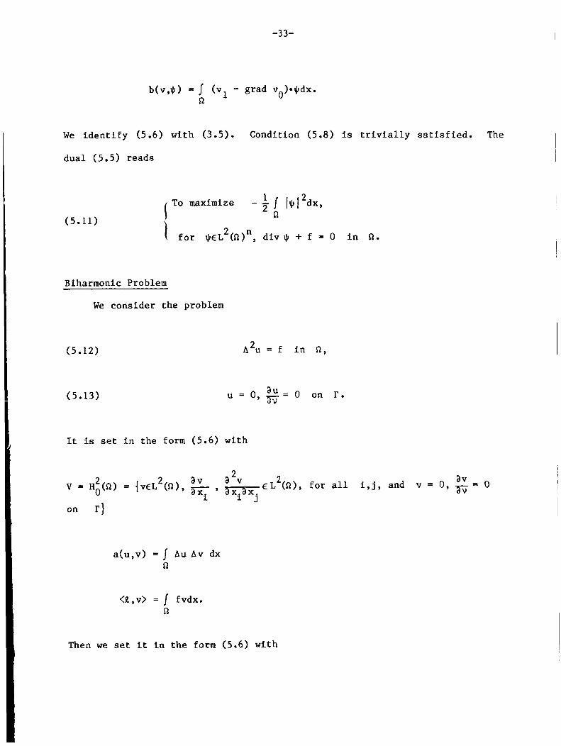
Biharmonic Problem
We cons ide r t h e problem
(5.12)
(5.13)
A u = f 2 i n 52,
a U u = 0, 0 on r .
It is set in t h e form (5.6) w i th
2 2 2 av 2
av= O a E L (Q), f o r a l l i , j , and v = 0, V = Ho(Q) = {VEL ( a ) , - axi ’ on r )
a ( u , v ) = 1 Au Av dx 52
<Il,v> = fvdx. s2
Then we set i t in t h e form (5.6) w i th

-34-
V = { u = {uo,ul}€X, u1 = Auo}
and f o r u = {uo,u l} , v = {vo,v 1 ) E X and $CY
a ( u , v ) = u v dx, <R,v> = / fvOdx n 1 1 n
b(v,$) = / (Avo - v )*$dx. 1 n
We i d e n t i € y (5.6) w i t h (3.5). Condi t ion (5.8) i s t r i v i a l l y s a t i s f i e d . The
d u a l (5.5) reads
( 5 . 1 4 )
1 To maximize - - I l$I2dx 2 Q
2 f o r $€L ( a ) , A$ = f i n n.
Problems involving t h e biharmonic appear i n e l a s t i c i t y and i n f l u i d mechanics
f o r t h e treatment of t h e Stokes problem by u t i l i z a t i o n of a stream funct ion .
5.c. Mixed and Hvbrid Elements
Once we have reduced Problem (5.1) t o (5.6), w e are n a t u r a l l y l e d t o
approximate t h i s las t problem, i .e. ,
- To f ind Xh, Yh , ah, bh, ch which approximate X , Y , a , b, c.
- Solve f o r each h a d i s c r e t e problem similar t o (5.6):

-35-
(5.15)
To f i n d uh€Xh, 19 EY such t h a t h h
"he xh v + b (v 4 ) = <Lh,vh> f o r a l l ah(uh' h h h ' h
bh(uh,qh) = 0, f o r a l l
F i n i t e element methods appear n a t u r a l l y i n t h e c o n s t r u c t i o n of t h e
spaces \ and Yh. We have more f l e x i b i l i t y than i n a n ord inary f i n i t e
and element method s i n c e w e can combine var ious f i n i t e elements f o r
f o r Yh. The major d i f f i c u l t y a r i s e s i n t h e v e r i f i c a t i o n of t h e c o n d i t i o n
(5.8) which l e a d s sometimes t o d e l i c a t e a l g e b r a i c ques t ions . A thorough
i n v e s t i g a t i o n of t h e i n f sup c o n d i t i o n f o r v a r i o u s f i n i t e e lements r e l a t e d t o
t h e Navier-Stokes equat ions can be found i n J. T. Oden and 0. P. J a c q u o t t e
[21 ] . I n some cases, t h e number f3 i n (5.8) corresponding t o t h e d i s c r e t e
case depends on h and tends t o 0 as h+O. In o t h e r c a s e s , t h e i n € sup
c o n d i t i o n does not hold i n t h e d i s c r e t e case and we can make i t t r u e by
i n o r d e r t o suppress t h e k e r n e l of t h e d i s c r e t e reducing t h e space
analogue Beh of B'; i n p r a c t i c e t h i s amounts t o a f i l t e r i n g procedure.
The most Eamous example is t h e c l a s s i c a l checkerboard i n s t a b i l i t y f o r a Stokes
problem corresponding t o t h e Q1 - Po element: Xh is a Q1 approximation
of H:(Ql2(n = 2) and Yh i s a Po approximation of L2(Q); t h e
f i l t e r i n g procedure is s tandard i n t h i s case; see a l s o t h e a n a l y s i s of t h e i n f
sup c o n d i t i o n i n Boland-Nicolaides [ 4 ] who show wi th a counter example t h a t
t h e b e s t va lue of f? i n t h i s ( d i s c r e t e ) case is of t h e form c h.
'h
'h
We w i l l not develop f u r t h e r t h i s q u e s t i o n h e r e s i n c e i t is t h e o b j e c t of
161 and o t h e r ar t ic les i n t h i s volume.

-36-
SPECIFIC APPLICATIONS
F i n i t e element methods have been t h e o b j e c t of many a p p l i c a t i o n s i n
mechanics and physics . We d e s c r i b e now some s p e c i f i c a p p l i c a t i o n s .
6. Navier-Stokes Equat ions
The n o t a t i o n s being t h e same as i n S e c t i o n 1 we cons ider t h e t i m e
dependent Navier-Stokes equat ions f o r v i scous incompress ib le f low i n a
domain Q
(6.2) d i v u = 0 i n n x (0,T)
( 6 - 3 ) u = U on r x ( 0 , T ) .
The unknowns are t h e v e l o c i t y v e c t o r u = u ( x , t ) and t h e p r e s s u r e
p = p ( x , t ) ; t h e volumic f o r c e s f and t h e boundary v e l o c i t y U (which may i 1 b o t h depend on t ime) are given. I
We r e c a l l t h a t from t h e mathematical p o i n t of view t h e i n i t i a l v a l u e 1
problem f o r t h e Navier-Stokes e q u a t i o n s , i.e., (6.1) - (6.3) supplemented by
a n i n i t i a l condi t ion
is w e l l set i n space dimension 2 (a c g). However, w e do not know y e t if
t h e same r e s u l t is t r u e i n space dimension 3 (QCl?), i.e., we do not know if

-37-
I
t h e c u r l v e c t o r remains bounded o r may become i n f i n i t e even i f t h e d a t a are
i n t e r v a l s of t i m e occur n a t u r a l l y i n the s tudy of t r a n s i e n t phenomena, while
" i n f i n i t e " i n t e r v a l s of time appear i n t h e s tudy of permanent regimes. For
i n s t a n c e if f and U are independent of t i m e , then i n some cases t h e solu-
r e g u l a r ; see f o r i n s t a n c e R. Temam [29].
I The i n t e r v a l of t i m e t h a t we consider may be f i n i t e o r i n f i n i t e . F i n i t e
t i o n u, p of (6.1) - ( 6 . 4 ) converges as t + m t o a s t a t i o n a r y s o l u t i o n ,
i.e., a s o l u t i o n of (1.7) - (1.9) . A s u f f i c i e n t cond i t ion f o r t h i s t o occur
i s t h a t t h e Reynolds number Re is s u f f i c i e n t l y small
where U, is a t y p i c a l v e l o c i t y of the flow and L* a t y p i c a l l e n g t h of
If Re i s l a r g e , t h e convergence t o a s t a t i o n a r y s o l u t i o n i s not 2 n .
guaranteed anymore. Rased on experimental. obse rva t ions r e l a t i v e t o turbu-
l ence , w e a c t u a l l y expec t t h a t u(* ,t), p(* , t ) do not converge anymore t o
t i m e independent s o l u t i o n s even i f the d a t a f,U are independent of t i m e .
From the numer i ca l po in t of view t h i s w i l l be t h e source of new d i f f i c u l t i e s
which have not ye t been explored and w i l l not be addressed he re (R. Temam
[301). Actua l ly the computing power t h a t is p r e s e n t l y a v a i l a b l e l e a v e s us a t
t h e th re sho ld of t h e occurrence of nons ta t ionary phenomena a t least i n space
dimension two.
a a I 2Typica l v e l o c i t i e s are provided by I, and f i n t h e form L * l V 2 norm(U),
a ., P i are The
L$1vB2 such t h a t t h e cor responding expres s ions have t h e dimension of a v e l o h t y . sum of t h e s e two v e l o c i t i e s is an appropr i a t e d e f i n i t i o n of U*.
norm(f), where a p p r o p r i a t e norms are cons idered and t h e I
I

-38-
Up t o now most of t h e numerical computations on t h e f u l l Navier-Stokes
e q u a t i o n s d e a l t with s t a t i o n a r y phenomena (and t r a n s i e n t phenomena). A t t h i s
l e v e l a major d i f f i c u l t y f o r t h e numerical s o l u t i o n of (6.1) - (6.4) (or (1.7)
- (1.9)) i s t h e handl ing of t h e f r e e divergence c o n d i t i o n s which i n t r o d u c e
complicated a l g e b r a i c c o n d i t i o n s i n t h e d i s c r e t e problem i f i t is not t r e a t e d
c o r r e c t l y . A c e r t a i n number of methods r e l a t e d t o o r independent from t h e
f i n i t e elements have been proposed t o overcome t h e d i f f i c u l t i e s a s s o c i a t e d
w i t h t h e condi t ion d i v u = 0.
a ) UtCl iza t ion of t h e Penal ty Method
The penal ty method which is due t o R. Courant [ l o ] in t h e contex t of con-
s t r a i n e d opt imiza t ion w a s appl ied t o t h e Navier-Stokes equat ions i n R. Temam
[ 2 5 ] , [26] . The i d e a which stems from t h e v a r i a t i o n a l form of t h e Stokes
problem ( s e e S e c t i o n 5) is t o treat t h e c o n d i t i o n d i v u = 0 as a c o n s t r a i n t
and t o "penalize" i t , i.e., t o r e p l a c e (6.1)(6.2) by
1 a t E
vAuc + (uC*V)uE - - V(V.ue) = f i n Qx (0,T) a u€ - -
where E: > 0 is a small parameter which is intended t o tend t o 0. It can
be proved [26] t h a t t h e s o l u t i o n of (6.3) - (6.5) converges t o t h a t of (6.1) - (6.4) when c+O. A f u l l asymptot ic expansion of u', p" i n terms of
e can even be obta ined i n t h e s impler case of Stokes flows [291.
The penal ty method has been a p p l i e d i n s e v e r a l ways by many a u t h o r s t o
t h e f i n i t e element approximations of t h e Navier-Stokes e q u a t i o n s , i n
p a r t i c u l a r with t h e mixed f i n i t e e lements (see Remark 5.1).

-39-
(1.9) o r t o the s o l u t i o n of t h e s t a t i o n a r y problems a r i s i n g from t i m e d i s -
c r e t i z a t i o n of ( 6 . 1 ) - ( 6 . 4 ) . In t hese cases, a n a r t i f i c i a l e v o l u t i o n problem
i s in t roduced whose s t a t i o n a r y s o l u t i o n is a l s o t h e s o l u t i o n of t h e s t a t i o n a r y
Navier-Stokes equat ion .
For i n s t a n c e , one can cons ider the a r t i f i c i a l e v o l u t i o n problem
L
1
I
~~
b) U t i l i z a t i o n of Algorithms: A r t i f i c i a l Time Dependence
This method a p p l i e s t o the s o l u t i o n of t h e s t a t i o n a r y problem (1.7) -
u h u + (u*V)u + grad p = f l aP a t - + a d i v u = 0
(a > 0) o r t h e equa t ions of s l i g h t l y compressible f l u i d s
( E - V A U + (u*V)u + grad p = f
\ - a P + a d i v u = 0. a t
In both cases t h e c o n d i t i o n d i v u = 0 is not imposed a t a l l times and
fo l lows simply from the p r o p e r t i e s of ( 6 . 6 ) and (6.7) f o r l a r g e t.
Consequently, o rd ina ry f i n i t e elements are used, i.e., f i n i t e elements not
c o n t a i n i n g the c o n d i t i o n d i v u = 0.
c > U t i l i z a t i o n of the P r o i e c t i o n Method
Th i s method in t roduced i n A. J. Chorin [81 and R. Temam [27 ] is connected
t o t h e f r a c t i o n a l s t e p method. It consists i n s o l v i n g t h e t i m e e v o l u t i o n of

-40-
(6.1) without (6.2) and then , more o r less f r e q u e n t l y , imposing (6.2) by
p r o j e c t i n g the v e l o c i t y obta ined on t h e f r e e divergence v e c t o r f i e l d s .
The time d i s c r e t i z a t i o n ( t ime mesh = A t ) when U = 0 is g iven by
-m m-1
A t - vbSm + (Gm*v)Gm = f m in R u - u
Gm = urn on T
-m and urn = Proj. of u which amounts t o say ing t h a t
m -m m u = u - grad q in 'd
d i v urn = 0 i n R
m m u * v _ (= normal component of u on r ) = 0 on r . i -
(6 .9)
m A l t e r n a t i v e l y set t - ing qm = A t n we can rewrite (6.9) as
m -m + grad n m = 0 i n R u - u
A t
(6.10) div urn = 0 i n Q
u * v _ = 0 on r , -
and pm provides a n approximation f o r t h e pressure . It is, however, a poor
approximation s i n c e i t s a t i s f i e s t h e fo l lowing nonphysical boundary c o n d i t i o n

t h a t w e i n f e r from (6.10):
(6.11)
-41-
m m In o r d e r t o de te rmine um i t is necessary t o a c t u a l l y compute q , IT , o r
is a s o l u t i o n of t h e Neuman problem which a t least t h e i r g r a d i e n t ; n
c o n s i s t s of (6.11) and
m
(6.12) Anm = - 1 d i v -m u . A t
It seems b e t t e r , f o r a more accu ra t e de t e rmina t ion of t h e p re s su re which
avo ids t h e undes i r ab le boundary l a y e r r e s u l t i n g from (6.11), t o cons ide r
as a u x i l i a r y func t ions and to compute t h e approximation pm of t h e m qm, = p r e s s u r e by us ing t h e boundary va lue problem
(6.13) p = $ ( u ) pm = $(urn)
t h a t we deduce d i r e c t l y from the Navier-Stokes equa t ions ; c f . [29]. A t t h i s
p o i n t one can e i t h e r use a D i r i c h l e t o r a Neuman boundary c o n d i t i o n f o r p
[ I51
Many o t h e r forms of (6.8)(6.9) can be a l s o considered: one can s p l i t t h e
o p e r a t o r s d i f f e r e n t l y , l eav ing f o r example some v i s c o s i t y i n (6.9), one can
u s e an e x p l i c i t scheme i n (6.8), o r one can s o l v e f o r t h e e v o l u t i o n (6.8) f o r
s e v e r a l s t e p s and perform t h e p r o j e c t i o n (6.9) p e r i o d i c a l l y only.
In a l l cases when t h e p r o j e c t i o n method is used w e need a space of f r e e
d ivergence v e c t o r f u n c t i o n s s o t h a t the p r o j e c t i o n (6.9) can be performed i n a
s a t i s f a c t o r y manner.

-42-
d ) U t i l i z a t i o n of free divergence f i n i t e element s p a c e s
The s imples t e lement , t h e piecewise l i n e a r ( P I ) f u n c t i o n on t r i a n g l e s ,
cannot be used s i n c e t h e c o n d i t i o n d i v u = 0 imposed on each t r i a n g l e l e a d s
t o too many a l g e b r a i c r e l a t i o n s and t h e spaces of d i s c r e t e d ivergence f r e e
P1 v e c t o r func t ions may be reduced t o t h e f u n c t i o n 0. One can e i t h e r impose
t h e cond€t ion d i v u = 0 "less o f t e n , " o r go t o more complicated elements
such as the nonconforming P1 element (F. Thomasset) o r P2, Q 1 , Q 2 , ..., elements.
7 . F l u i d S t r u c t u r e I n t e r a c t i o n s
I n many i n d u s t r i a l f i e l d s of i n t e r e s t , i n c l u d i n g t h e space i n d u s t r y ,
e n g i n e e r s a r e confronted wi th f l u i d s (water, o i l , kerosene , g a s e s , ...) i n t e r a c t i n g wi th s t r u c t u r e s ( t a n k s , c o n t a i n e r s , o b s t a c l e s , ...) along a more
o r less extended area.
I n some cases deformations of t h e s t r u c t u r e may be f a i r l y important and
even a f f e c t t h e motion of t h e f l u i d ; e n g i n e e r s have then t o s o l v e problems
i n c l u d i n g a coupl ing between f l u i d displacements and e l a s t i c deformations of
t h e s t r u c t u r e .
We descr ibe h e r e t h e i n t e r a c t i o n between a f r e e s u r f a c e f l u i d and t h e
s t r u c t u r e , assumed t o be e las t ic , which c o n t a i n s i t , i n a n e x t e r n a l f o r c e
f i e l d . We fo l low J. Mathieu [13] and J. Mathieu, e t a l . [ 2 0 ] , who computed
t h e t r a n s i e n t s i m u l a t i o n of such a process wi th t h e BACCHUS Code.
I
7.a. The Arbi t ra ry Lagrange-Euler (ALE) Descr ip t ion
We consider a moving domain n F ( t ) deforming wi th v e l o c i t y
w = w ( x , t ) , and f i l l e d wi th an incompressible f l u i d of ( c o n s t a n t ) d e n s i t y

-43-
P which obeys t h e Navier-Stokes equat ions. We cons ider a l s o a second
domain R S ( t ) made of e las t ic m a t e r i a l and l i m i t i n g 52 . The f l u i d is
l i m i t e d by a free s u r f a c e S and t h e contac t s u r f a c e T = a ( t ) wi th Q.
F
S
The equat ions are
I I
(7.1)
F F F vF + ( (vF - w)V)v } = d i v B + pFfF i n 51 {E
F div v = 0
S S a v - d i v as + p s f s i n R at-
where
- - - 6p - it + ( w . 0 ) ~ 6 t
i s t h e convection d e r i v a t i v e a s s o c i a t e d wi th t h e
vec tor f i e l d w
i v = t h e v e l o c i t y f i e l d i n Qi
B = t h e stress t e n s o r i n Qi
p i = d e n s i t y i n R (cons tan t i n RF)
i
i
f = e x t e r n a l f o r c e s
J = Jacobian of t h e mapping Rs(0)+Rs(t).

-44-
The ALE d e s c r i p t i o n is determined by t h e a c t u a l v e l o c i t y f i e l d w which
is def ined as fol lows:
w = 0 i n a n i n t e r n a l e u l e r i a n r e g i o n
w = vF on t h e f r e e s u r f a c e S ( t )
w = vs on t h e w e t p a r t of t h e w a l l n ( t ) .
F igure 7.1
The c o n s t i t u t i v e laws are
F F F t u = v [ p + (EV 1 1 + p i
f o r t h e f l u i d , v = t h e k inemat ic v i s c o s i t y , p = t h e h y d r o s t a t i c p r e s s u r e ,
and
S u S ( t ) = F ( t ) z ( t ) F ( t I t
P ( 0 )

-45-
i
4
f o r t h e s o l i d where 2
i s t h e g r a d i e n t of t h e mapping
Cs t h e s tandard second P i o l a Kirchhoff t e n s o r , F ( t )
S ns(0)+ns( t ) , and ~ ( 0 ) = u ( 0 ) = 0 .
The boundary c o n d i t i o n s are as fol lows :
- On t h e s t r u c t u r e , displacements a re given on some p a r t
r ( t ) of a Q s ( t ) \ r ( t ) and normal stresses are g iven along t h e remaining
p a r t of a n s ( t > \ n ( t > .
- On t h e w e t p a r t of t h e w a l l , n ( t ) , w e have no c a v i t a t i o n ,
U
2 t h e normal on
a long t h e w a l l
- TI, and we have a p a r t i a l s l i p c o n d i t i o n of t h e f l u i d
and f i n a l l y t h e normal stresses are cont inuous
F S (a - a >.y = 0.
The d i s c r e t i z a t i o n of t h e problem is made wi th a f i n i t e e lement
d i s c r e t i z a t i o n in space, providing an easy handl€ng of t h e complex geometr ic
c o n f i g u r a t i o n s which are caused by l a rge displacements . The elements are of
degree one f o r t h e v e l o c i t i e s (= P1 f o r t r i a n g l e s , Q1 f o r r e c t a n g l e s , Q1
t r a n s p o r t e d Q1 f o r q u a d r i l a t e r a l s ) , and piecewise c o n s t a n t s f o r t h e hydro-
s t a t i c pressure.
A one-step e x p l i c i t f i n i t e d i f f e r e n c e scheme is used i n t i m e . T h i s
scheme is s u b j e c t t o t h e u s u a l s t a b i l i t y c o n d i t i o n s l i m i t i n g t h e t i m e s t e p .

-46-
The c r i t e r i a taken i n t o account are
- f r e e su r face wave and v iscous wave s t a b i l i t y i n t h e f l u i d
- a c o u s t i c wave s t a b i l i t y in t h e s t r u c t u r e .
Because of the more d r a s t i c l i m i t a t i o n due t o t h e s t a b i l i t y c r i t e r i o n i n t h e
s t r u c t u r e , a subcycl ing procedure is used f o r t h e s t r u c t u r e c a l c u l a t i o n .
A mesh a d a p t a t i o n procedure is necessary. A t each f l u i d - c a l c u l a t i o n
s t e p , t h e f r e e s u r f a c e has t o be r epos i t i oned . The d isp lacements of t h e f r e e
s u r f a c e and of t h e i n t e r f a c e between t h e f l u i d and t h e s t r u c t u r e induce a
modi f i ca t ion of t h e mesh i n t h e mixed Lagrange-Euler r eg ion and p o s s i b l y a
mod i f i ca t ion of t he E u l e r reg ion (when i t s boundary i n t e r s e c t s t h e free
s u r f a c e o r t he w a l l ) o r a degeneracy of some element. Thus a rezoning is
au tomat i ca l ly performed dur ing t h e c a l c u l a t i o n . The rezoning is a l s o
necessary on n ( t ) s i n c e any node belonging t o aQF(t)naQS(t) should be
a t the same t i m e a v e r t e x of some e l e m e n t of and of some element Q s ( t > - of Q F ( t ) .
A sample two-dimensional c a l c u l a t i o n i s shown on Figure 7.2:

-47-
-47-
t = 0 DS and S are given.
The internal mesh will be automatically designed.
t = 0,2 The bottom of the tank is in a compressive phasis.
Notice the behavior of the velocity fields on n: double-valued with normal component continuity.
t = 0,3 The bottom of the tank has entered an expansive phasis.
t = 0,5 The tank has reached large enough deformations.
The free-surface tends to stabilize towards the horizontal. Notice the modification of the mesh in DF.
Figure 7 . 2

-48-
8. Three Dimensional Eu le r Equat ions
The f i n i t e element method has been a p p l i e d t o t h e computation of t h e
s o l u t i o n of t h e Euler equat ions . We d e s c r i b e h e r e t h e l a tes t r e s u l t s i n C.
H. Rruneau, e t a l . [ 7 1 , which concern t h e computation of s t eady v o r t e x flows
p a s t a f l a t p l a t e a t h igh ang le of a t t a c k .
8.1. Desc r ip t ion of t h e Problem
The purpose of t h e computations i n [ 7 ] is t o i n v e s t i g a t e t h e developments
of v o r t i c e s a t t h e t i p of t h e p l a t e and t h e i r p ropagat ion a f t e r t h e t r a i l i n g
edge. I n t h e computations, t he p l a t e has no t h i c k n e s s and w e expect a s t r o n g
v o r t e x s t r u c t u r e t o develop a t the t i p of t h e p l a t e ; i t is not p o s s i b l e t o use
p o t e n t i a l equat ions and t h e f u l l Euler equa t ions are necessary . Fo r t h e
computations, t he p l a t e i s imbedded i n a 3-D r e c t a n g u l a r domain as shown on
F igure 8.1; t h e a spec t r a t i o is 0.5 and t h e ang le of inc idence i s a = 15’
o r a = 30’. Figure 8.1 shows only ha l f of t h e p l a t e s i n c e symmetry wi th
respect t o t h e y v a r i a b l e i s assumed.
+ ~ ‘a The incoming flow is g iven by q, = (u,, v,, w,) = (4, cosa , 0, L
2 qm s i n a ) , a as above, and Ma t h e Mach number a t i n f i n i t y , M, = - 2 ’ - 2
I n t h e s e computations, t h e flow is subsonic , 2 ‘t
a, = (Y - 1 ) ( H -
M, = 0.7.

-49-
Figure 8.1
E u l e r Equat ions
They are w r i t t e n i n conserva t ive form
Conservat ion of mass
Conservat ion of momentum
Bernoulli’s equat ion
where P , q -s = (u ,v,w), p r ep resen t s r e s p e c t i v e l y the d e n s i t y , the
v e l o c i t y vec to r , and t h e p re s su re ; H i s t h e t o t a l and y t h e r a t i o of
s p e c i f i c heats.

-50-
Boundary Conditions
The boundary c o n d i t i o n s on t h e p l a t e are easy; t h e tangency c o n d i t i o n on
t h e p l a t e (plane z = 0) reads w = 0, and t h e symmetry c o n d i t i o n i s v = 0
on y = 0. On t h e c o n t r a r y , t h e boundary c o n d i t i o n s a t t h e l i m i t s of t h e
domain are not easy , e s p e c i a l l y downstream where i t should a l low t h e v o r t e x t o
go through the e x i t plane.
The flow v a r i a b l e s have been set t o the, f r e e s t r e a m va lues a t t h e incoming
boundaries (x = xo, z = z o ) , and no c o n d i t i o n w a s imposed a t t h e e x i t
boundaries (x = xl, z = zl) so t h a t t h e va lues t h e r e are computed from t h e
v a r i a t i o n a l formulat ion. Due t o t h e u t i l i z a t i o n of a least square method,
t h i s amounts simply t o r e q u i r i n g t h a t t h e Eirst o r d e r equat tons be s a t i s f i e d
a t those boundaries (see [ 7 ] f o r a d i s c u s s i o n of t h e boundary c o n d i t i o n s ) .
A t y = y1 t h e far f i e l d condi t ions v = 0 i s used.
8.2 The Numerical Method and t h e Numerical R e s u l t s
The equat ions are so lved i t e r a t i v e l y as fo l lows:
- A f ixed poin t a lgor i thm is based on equat ion (8.2), computing t h e
d e n s i t y when u, v , w, p are known.
- The nonl inear system (8.1) provides u , v, w, p , us ing t h e va lue of
p from t h e previous s t e p of t h e i t e r a t i o n . This system is l i n e a r i z e d by
Newton’s method w i t h l i n e a r i z e d v a r i a b l e s u, v, w, p.
- The sys t em f o r u , v, w, p i s d i s c r e t i z e d by a n a p p r o p r i a t e Q1
f i n i t e element method ( d i s c r e t i z a t i o n of t h e c o n s e r v a t i v e v a r i a b l e s
pu, pv, p w , ...) and t h e system i s so lved by a least square method.
“ N N
“ N N
Figures 8.2 and 8.3 show a sample of t h e d i s c r e t i z a t i o n g r i d . F i n a l l y ,
F i g u r e s 8.4 t o 8.6 show t h e c r o s s flow v e l o c i t i e s a t 70%, 90%, and 110% of t h e
p la te

-51-
U ! ! ! ! ! ! I I -1
& I ! ! ! ! I
U ! ! ! ! : ! I
Figure 8.2
I
I
1.
T T T T T m T T I T T T i T
Figure 8 . 3
T
1 Figure 8.4

-52-
I T 1 1 1 1 \ \
i i . \ s . . . I . - . . .
// 11
T TTTTlnllllnlnrllllTTTT T T 1 T T
Figure 8.5
1 1 I 1 1 1
i i : : . . - . . . 1 4
I t a \ . \ .. . *
TTTT-TTT T T Figure 8.6

-53-
FUTURE DEVELOPMENTS
The advantages of FEM are w e l l known. I n p a r t i c u l a r
- a c c u r a t e and automating f i t t i n g of complicated geometries.
- lowering ( d i v i d i n g by 2) t h e order of t h e d i f f e r e n t i a l o p e r a t o r s t h a t
appea r , due t o t h e u t i l i z a t i o n of weak formula t ions .
- avoid ing t h e d i s c r e t i z a t i o n of the boundary cond i t ions of t h e Neuman
type which d i sappea r i n t h e weak formulations.
The inconveniences are
- t h e need of a t r i a n g u l a t i o n program f o r domains which has t o be w r i t t e n
once f o r a l l but i s a d iscouraging pre l iminary s t e p f o r t h e nonexpert.
- t h e computational c o s t s which by no way can compete with the achieve-
ments of m u l t i g r i d and spectral methods.
However, t he m u l t i g r i d and s p e c t r a l methods a t t a i n t h e i r op t imal
e f f i c i e n c y f o r r e c t a n g u l a r domains. It is then conce ivable t h a t a combination
of FEM and m u l t i g r i d and spectral methods i n r e l a t i o n wi th domain decomposi-
t i o n and p a r a l l e l computation can prove t o be e f f i c i e n t .
9. Domain ~ecomDos i t ion : Remarks on Future DeveloDments
The domain decomposition which l i e s a t the foundat ion of t h e FEM can
appear t o be, i n a d i E f e r e n t form, d i r e c t l y r e l a t e d t o f u t u r e developments i n
t h e method. Besides t h e geometr ica l c o n s i d e r a t i o n s , t h e r e are many o t h e r good
reasons f o r decomposing t h e s o l u t i o n of a boundary va lue problem i n a l a r g e
domain i n t o t h e s o l u t i o n of similar problems i n subdomains. L e t us mention
some of them:
-54-
a ) Adaptive meshes
Adaptive meshes may be s u i t a b l e f o r geometr ica l o r a n a l y t i c a l reasons.
For i n s t a n c e , t h e f i t t i n g of a curved domain wi th elements of d i f f e r e n t n a t u r e
which are more a p p r o p r i a t e in v a r i o u s p a r t s of t h e domain. The ref inement of
t h e mesh i n reg ions where t h e s o l u t i o n s are s i n g u l a r o r near ly s o (boundary
l a y e r s , shocks, f r o n t f lames, e t c . ) a l low f o r e x t r a computational e f f o r t t o be
concentrated i n such reg ions . Thus f i n i t e e lements of d i f f e r e n t types and
s i z e s may be used i n v a r i o u s p a r t s of a domain, and a d i f f e r e n t t rea tment of
t h e d i f f e r e n t reg ions can be usefu l .
b) Physical Motivat ions
Phys ica l phenomena of a d i f f e r e n t na ture may occur i n d i f f e r e n t r e g i o n s ,
and t h e s e regions should not be t r e a t e d i n a s imilar manner. For i n s t a n c e i n
a e r o n a u t i c s
- a turbulence model i s necessary near t h e a i r f o i l
- t h e Navier-Stokes e q u a t i o n s wi th v iscous e f f e c t s and without t u r b u l e n c e
are necessary a t a c e r t a i n d i s t a n c e but not t oo f a r
- the Euler equat ions ( i .e . , no viscous e f f e c t ) are s u f f i c i e n t f a r from t h e
a i r f o i l .
S i m i l a r s i t u a t i o n s occur i n combustion o r i n s o l i d mechanics and l ead
n a t u r a l l y to t h e decomposition of t h e whole domain i n t o smaller ones.
1 I c) P a r a l l e l Computation
The technology of computers w i l l a p p a r e n t l y move more and more toward
p a r a l l e l computation. The decomposition of a domain i n t o subdomains on which
t h e computations are made s imultaneously i s a p p r o p r i a t e f o r p a r a l l e l computa-

-55-
t i o n s .
all t h e subdomains t o ensure a c o r r e c t i n t e r a c t i o n of t h e subdomains.
The d i f f i c u l t y i s then t o p e r i o d i c a l l y s y n t h e s i z e t h e informat ion from
Figure 9.1
I f t h i s
technique is s a t i s f a c t o r i l y mastered, then one can cons ider , as has a l r e a d y
been done ( s e e f o r i n s t a n c e [13][23][191), combining t h e advantages of FEM and
s p e c t r a l and m u l t i g r i d methods by using domain decomposition as suggested i n
F i g u r e 9.1. This has a l r e a d y been done, but t h e g o a l i s t o g e t as c l o s e as
p o s s i b l e t o t h e performance of t h e f a s t methods.
.-- A t tha -..- n r n c n n t r..-V-'.- t l m n --...I wnrt ...,..._ 5s bgizg dene de-25z d ~ ~ ~ ~ p ~ ~ 5 ~ ~ ~ f i .

-56-
CONCLUDING ReMARK
The FEM cannot pre tend t o be t h e b e s t method i n a l l s i t u a t i o n s , but i t
has proved to be a n e f f i c i e n t and performant method i n many cases and can hope
t o be t h e ob jec t of f u t u r e i n t e r e s t i n g developments. R. Feyman says i n h i s
book [ 1 2 ] t h a t he was a b l e t o s o l v e some problems t h a t o t h e r people could not
s o l v e j u s t because he had some t o o l s i n his box t h a t o t h e r s d i d not have. It
would be too bad not t o have t h e FEM t o o l i n h i s box of numerical methods.

-57-
BgFERENCES
[ l ] J. H. Argyr is , "Energy theorems and s t r u c t u r a l a n a l y s i s , part I:
General Theory," A i r c r a f t Engineering, 26, 1954, pp. 347-356, 383-387,
394, 27, 1955, pp. 42-58, 80-94, 125-134.
[ 2 ] I. Babuska, "The f i n i t e e l emen t method wi th Lagrangian m u l t i p l i e r s , "
Numer. Math., 20, 1973, pp. 179-192.
[3 ] M. Bercovier , "Pe r tu rba t ion of mixed v a r i a t i o n a l problems," App l i ca t ion
t o mixed f i n i t e e l emen t methods, RAIRO Anal. Num., 12, 1978, pp. 211-
236.
[4 ] J. Boland and R. N ico la ides , "Stable and semis t ab le low o r d e r f i n i t e
elements f o r v i scous flows,11 Un ive r s i ty of Connect icu t , p r e p r i n t , 1984.
[ 5 ] F. Brezz i , "On t h e e x i s t e n c e , uniqueness and approximation of saddle-
po in t problems a r i s i n g from Lagrangian M u l t i p l i e r s , " RAIRO-Analyse
Numerique, 8, 1974, pp. 129-151.
[ 6 ] F. Brezz i , " F i n i t e element approximations of t h e Von Karm5n equa t ions , "
RAIRO Numer. Anal., 12, No. 4 , 1978, pp. 303-312.

-58-
[ 7 ] C. H. Rruneau, J. J. C h a t t o t , J. Laminie, and R. Temam, "Computation of
vor tex flows past a f l a t p l a t e a t h igh angle of a t t a c k , " i n Proceedings
of the 10th I n t e r n a t i o n a l Conference on Numerical Methods i n F l u i d
Mechanics (Peking 1986), Lec ture Notes i n Phys ics , Springer-Verlag, New
York, 1987.
[ 8 ] A. J. Chorin, "A numerical method f o r s o l v i n g incompressible v i s c o u s
flow problems," J. Comp. Phys., 2, 1967, pp. 12-26.
[ 9 ] P. G. C iar le t , The F i n i t e Element Method f o r E l l i p t i c Problems, North-
Holland, Amsterdam, 1978.
[ l o ] R. Courant, "Var ia t iona l methods f o r t h e s o l u t i o n of problems of
equi l ibr ium and v i b r a t i o n s , " Bull . h e r . Math. SOC., 49, 1943, pp. 1-23.
[ l l ] I. Ekeland and R. Temam, Convex Analysis and V a r i a t i o n a l Problems,
North-Holland, Amsterdam, 1976.
[12] R. Feyman, Sure ly You're Joking M r . Feyman, W. W. Norton & Company, New
York, 1985.
[ 131 B. Gest, "Methode de r e s o l u t i o n r a p i d e des systemes l i n 6 a i r e s , " T h e s i s ,
Labora to i re d'bnalyse Numgrique U n i v e r s i t g P a r i s Sud, Orsay, 1985.
1141 V. G i r a u l t and P. A. Raviar t , F i n i t e element methods f o r t h e Navier-
Stokes e q u a t i o n s , Spr inger S e r i e s i n Computational Mathematics, 1986.

-59-
[17 ] J. Leray, "Essais s u r les mouvements p lans d'un l i q u i d e visqueux que
[15] P. M. Gresho and R. L. Sani , "On p r e s s u r e boundary cond€t ions f o r t h e
incompress ib le Navier-Stokes equat ions," U n i v e r s i t y of Colorado,
Boulder, p r e p r i n t , 1986.
[16] J. Leray, "Etude de d i v e r s e s liquations i n t e g r a l e s non l i n e a i r e s e t de
que lques problemes que pose l'hydrodynamique," J. Math. Pures Appl., 12,
1933, pp. 1-82.
l i m i t e des p a r o i s , " J. Math. Pures Appl., 13, 1934, pp. 331-418.
[18] J. Leray, "Essai s u r l e mouvement d'un l i q u i d e empl i ssant l'espace,"
Acta Math., 53, 1934, pp. 193-248.
[ 191 C. Lesartre, Thes is i n prepara t ion , L a b o r a t o i r e d'Analyse Numerique,
Univers i te ' P a r i s Sud, Orsay, 1987.
[20] J. Math€eu, P. Ravier , J. Boujot, P. Gendre, M. H i t t i n g e r , " I n t e r a c t i o n
between s t r u c t u r e and f r e e sur face f l u i d wi th l a r g e displacements of by
f i n i t e e lements ," i n Proceedings of t h e 10th I n t e r n a t i o n a l Conference on
Numerical Methods i n F l u i d Mechanics (Peking 1986), Lec ture Notes i n
Phys ics , Springer-Verlag, New York, 1987.
[211 J. T. Oden and 0. P. J a c q u o t t e , " S t a b i l i t y of some mixed f € n i t e element
methods f o r S t o k e s i a n flows," Computer Methods i n Applied Mechanics and
Engineer ing, 43 , 1984, pp. 231-248.

-60-
[ 2 2 ] J. Periaux, First International Conference on Industrial and Applied
Mathematics, Paris, June 1987.
[ 2 3 ] B. Ravier, "Methode de decomposition des domaine," Thesis, Laboratoire
d'Analyse Numerique, Universitg Paris Sud, Orsay, 1986.
[ 2 4 ] B. Scheurer, "Existence et Approximation de points selles pour certains
problemes nonlineaires," RAIRO-Analyse Numerique, 11, 1977, pp. 369-400.
[ 2 5 ] R. Temam, "Sur l'approximation des solutions des Gquations de Navier-
Stokes," C. R. Ac. Sc. Paris, S6rie A, 262, 1966, pp. 219-221.
[ 2 6 ] R. Temam, "Une methode d'appraximation de la solution des 6quations de
Navier-Stokes," Bull. SOC. Math. France, 98, 1968, pp. 115-152.
[ 2 7 ] R. Temam, "Sur l'approximation de la solution des equations de Navier-
Stokes par la methode des pas fractionnaires 11," Arch. Rat. Mech.
Anal., 33, 1969, pp. 377-385.
[ 2 8 ] R. Temam, Numerical Analysis, Reidel Pub. Comp., Dordrecht, Holland,
1973.
[ 2 9 ] R. Temam, Navier-Stokes Equations, 3rd revised edition, North-Holland,
Amsterdam, 1984.

-6 1-
[301 R. Temam, "Chaos i n Fluids," Lecture a t the SIAM National Meeting,
Boston, July 1986.
[31] R. Temam, Lecture a t the INRIA-SIAM-SOCAI Workshop on Domain
Decomposition, Par i s , Proceedings to be published by SIAM, Philadelphia,
January 1987.
[32] F. Thomasset, Implementation of Fini te Element Methods for Navier-Stokes
Equations, Springer Series i n Comp. Phys. , 1981.
[33 ] 0. C. Zienckiewicz, The F in i t e Element Method i n Engineering Science,
MacGraw-Hill, London, 1971.

Standard Bibliographic Page
=Report No. NASA CR-178222 ICASE Report No. 86-77
2. Government Accession No.
7. Author(s)
Roger Temam
17. Key Words (Suggested by Authors(s))
3. Performing Organization Name and Address I n s t i t u t e f o r Computer App l i ca t ions i n Sc ience
Mail Stop 132C, NASA Langley Research Center Hampton, VA 23665-5225
and Engineering
12. Sponsoring Agency Name and Address
18. Distribution Statement
Na t iona l Aeronautics and Space Adminis t ra t ion Washington. D.C. 20546
19. Security Classif.(of this report) 20. Security Classif.(of this page) 21. No. of Pages Unc la s s i f i ed U n c l a s s i f i e d 63
15. Supplementary Notes
Langley Technical Monitor: J. C. South
22. Price A04
F i n a l ReDort
3. Recipient's Catalog No.
5 . Report Date
November 1986 6. Performing Organization Code
8. Performing Organization Report No.
86-77 10. Work Unit No.
11. Contract or Grant No. NAS1-18107
13. Type of Report and Period Covered
Con t rac to r Report 14. Sponsoring Agency Code
_-
16. Abstract
The f i n i t e element methods (FEM) have proved t o be a powerful technique f o r the s o l u t i o n of boundary va lue problems a s s o c i a t e d w i t h p a r t i a l d i f f e r e n t i a l equat ions of e i t h e r e l l i p t i c , p a r a b o l i c , o r hype rbo l i c type . They a l s o have a good p o t e n t i a l f o r u t i l i z a t i o n on p a r a l l e l computers p a r t i c u l a r l y i n r e l a t i o n t o t h e concept of domain decomposition.
This r e p o r t is in tended as a n i n t r o d u c t i o n t o t h e FEN f o r t h e n o n s p e c i a l i s t . It c o n t a i n s a survey which i s t o t a l l y nonexhaus t ive , and i t a l s o c o n t a i n s as a n i l l u s t r a t i o n , a r e p o r t on some new r e s u l t s concern ing two s p e c i f i c a p p l i c a t i o n s , namely a f r e e boundary f l u i d - s t r u c t u r e i n t e r a c t i o n problem and t h e Euler e q u a t i o n s f o r i n v i s c i d flows.
f i n i t e elements, Eulcr equa t ions s t r u c t u r a l mechanics
64 - Numerical Analys is 05 - A i r c r a f t Design, Tes t ing ,
and Performance
For sale by the National Technical Information Service, Springfield, Virginia 22161 NASA-Langley, 1987