A University of Sussex DPhil thesis 

Available online via Sussex Research Online: 

http://sro.sussex.ac.uk/   

This thesis is protected by copyright which belongs to the author.   

This thesis cannot be reproduced or quoted extensively from without first obtaining permission in writing from the Author   

The content must not be changed in any way or sold commercially in any format or medium without the formal permission of the Author   

When referring to this work, full bibliographic details including the author, title, awarding institution and date of the thesis must be given 

Please visit Sussex Research Online for more information and further details   

Supply Response and Market Imperfections: the Implications for

Welfare Analysis

Antonio Martuscelli

Submitted for the degree of Doctor of Philosophy Department of Economics University of Sussex January 2013

Declaration I hereby declare that this thesis has not been and will not be submitted in whole or in part to another University for the award of any other degree. Signature:

Antonio Martuscelli

iii

UNIVERSITY OF SUSSEX

Antonio Martuscelli, Doctor of Philosophy

Supply Response and Market Imperfections: the Implications for Welfare Analysis

Summary

In this thesis we investigate the supply side of farm households in the Tanzanian region of Kagera and incorporate the results into a welfare analysis of price shocks and trade policy options. The first chapter discusses the relevance of agriculture as an engine of growth and poverty reduction and introduces the context and the data used for the empirical analysis. The second chapter tests for separability of the households demand and supply sides and then estimates supply functions for the main crops. We find that separability cannot be rejected for this sample and that farmers are only partially responsive to price incentives. The third chapter analyses the role of market participation decisions and transaction costs for food supply. We find that transaction costs play an important role in households supply decisions. Moreover, we show that there is a positive although small supply response to prices once controlling for the unresponsiveness of self-sufficient households. The fourth chapter extends the standard welfare impact analysis of price shocks to incorporate supply and demand responses as well as the role of market participation and transaction costs. We find that the results are sensitive to the introduction of households’ output, wage and consumption responses.

iv

Acknowledgements My greatest thanks go to my supervisor, Alan Winters. He has been over the years a constant source of ideas and precious advices. I am really grateful to him for carefully reading all the drafts passed by his hands offering always important comments and suggestions.

I owe a lot to all the other members of the economics department. In particular to Andy Newell and Andy McKay who gave me the opportunity to teach several courses over the years; to Michael Gasiorek and Peter Holmes who gave me the opportunity to be involved in a number of interesting projects; to Barry Reilly for his invaluable econometrics suggestions.

My thanks go also to Jean-Marie Baland and all the people at the University of Namur who gave me precious comments on early drafts of the thesis.

I am grateful to all the attendants at the Pacdev 2012 conference at the University of California, Davis, the CRED workshop at the University of Namur, the LICOS seminar at the University of Leuven and the Economics PhD conference at the University of Sussex for their comments and suggestions.

I received a great help from all the fellow PhD students at Sussex. Thanks to Gonzalo, Marinella, Javi, Paola, Giulia, Max, Kalle, Marta, Alvaro and Jairo for enriching life at Sussex both inside and outside the university premises. A great joy has been spending time with Luisa and Maria whose company I have really appreciated.

Very great thanks go to Roxane. Without your presence and support my life in this period would not have been so enriching and fascinating.

Last but absolutely not least a great thank to my parents Ezio and Cristina who made this possible with their unconditional support. No words would ever be enough to express my gratitude.

v

Contents

List of Tables vii List of Figures viii Acronyms ix Introduction 1 1 Rural development and the Kagera region 4

1.1 Introduction 4

1.2 The role of agriculture in economic development 4

1.3 The Kagera region 18

1.4 The KHDS dataset 24

1.5 Evolution of welfare and agriculture 32

Appendix 1 Estimating conversion factors for prices and quantities 41

2 Agricultural supply response, transaction costs and separability: evidence from Tanzania 45

2.1 Introduction 45

2.2 Conceptual background 46

2.3 Empirical tests for separability: a review of the literature 62

2.4 Separability and supply response 69

2.5 Conclusions 98

3 Supply response, market participation and transaction costs in food markets: evidence from a Tanzanian panel 99

3.1 Introduction 99

3.2 Literature review 101

3.3 Theoretical framework 106

3.4 Discrete choice models for longitudinal panel data 115

vi

3.5 Supply response and market participation: a panel selectivity model with an

ordered probit selection rule 122

3.6 Empirical analysis 128

3.7 Robustness checks 141

3.8 Conclusions 147

Appendix 2 Food supply pooled estimation 148

Appendix 3 Stata routine for the MSL estimation 149

4 Analysing the impact of trade liberalization and price shocks in rural economies 153

4.1 Introduction 153

4.2 Trade, poverty and income distribution: the links 156

4.3 Methodologies in assessing the welfare impact of trade reforms 161

4.4 Households’ behavioural response: a medium term impact analysis 169

4.5 Estimation of demand, supply and wage-income elasticities 175

4.6 Empirical analysis: evaluation of trade reforms and price shocks 184

4.7 The role of market participation and transaction costs 196

4.8 Conclusions 204

Bibliography 206

vii

List of tables 1.1 Evolution of welfare 1991/2004 1.2 Evolution of the agricultural sector 1991/2004 1.3 Price regressions 2.1 Descriptive statistics KHDS 2.2 Descriptive statistics KHDS (cont.) 2.3 Variables description 2.4 Separability test 2.5 Coffee supply 2.6 Food supply 2.7 SUR with fixed effects 2.8 Evolution of supply response: FE with interaction terms 2.9 Wooldridge test for selectivity 2.10 separate FE estimation 3.1 Descriptive statistics 3.2 Summary statistics of main variables 3.3 Results 3.4 Average partial effects ordered probit 3.5 Decomposition of unconditional marginal effects 3.6 Controlling for risk, credit access and land quality 3.7 Excluding buying and selling households 3.8 Three waves estimation 3.9 Food supply pooled estimation 4.1 Almost Ideal Demand System 4.2 Own, cross-price and income elasticities 4.3 Wage-income elasticities 4.4 Demand, supply and wage-income elasticities 4.5 Price change scenarios 4.6 Welfare impact 4.7 Demand, supply and wage-income elasticities 4.8 Welfare impact food price shock 4.9 Net-buyers, self-sufficient and net-sellers welfare impact food price shock

viii

List of figures 1.1 Kagera region, Tanzania 1.2 Kagera region, districts and roads 1.3 Expenditure distribution 1991/2004 1.4 Evolution of agriculture 1.5 Crop mix and specialization 1.6 Commercialization patterns 3.1 Net-sellers and net-buyers 3.2 Households’’ market position 3.3 Indirect utility function 3.4 Fixed transaction costs 3.5 Supply function 4.1 Shares of food, coffee and agricultural wage income 4.2 Shares of total output, auto-consumption and food net-consumption ratio 4.3 Doha scenario 4.4 Full liberalization scenario 4.5 Food price scenario 4.6 Coffee price scenario 4.7 Baseline and transaction costs scenarios: first-order impact 4.8 Baseline, market participation and transaction costs scenarios: full-model impact

ix

Acronyms AIDS Almost Ideal Demand System

CGE Computable General Equilibrium

FIML Full Information Maximum Likelihood

FOC First Order Condition

FTC Fixed Transaction Cost

GDP Gross Domestic Product

IFI International Financial Institution

KHDS Kagera Health and Development Survey

MSL Maximum Simulated Likelihood

NBS National Bureau of Statistics

NLSUR Non-Linear Seemingly Unrelated Regressions

OLS Ordinary Least Square

PSU Primary Sampling Unit

PTC Proportional Transaction Cost

SSA Sub-Saharan Africa

SUR Seemingly Unrelated Regressions

TCMB Tanzania Coffee Marketing Board

TZS Tanzanian Shilling

1

Introduction

This thesis analyses the production decisions of rural households in the Tanzanian

region of Kagera. The main aim of the study is to improve our understanding and

provide new empirical evidence on how households’ supply decisions are formed in a

context potentially characterized by the presence of market imperfections. The results of

this analysis are then applied to develop a more comprehensive framework to assess the

welfare impact of price shocks.

The main motivation behind the study derives from the realization that the literature on

the impact of price shocks on household welfare has not focused sufficiently on the

supply side of the story when dealing with rural agricultural-based contexts. While the

literatures on both households’ decisions on the one hand and on the welfare impact of

different kind of shocks and policies on the other hand are extended and long dated the

two are not often integrated. This thesis is intended to progress this integration.

The first chapter is an introductory chapter that reviews the literature on the role of

agriculture in the development process. It puts the subsequent chapters into a broad

context which sees agriculture and rural development as an important part of a

sustainable growth strategy. In this introductory chapter we also describe the main

characteristics of the region that is the focus of the empirical analysis and describe the

dataset used in the analysis.

In the second chapter we start the empirical analysis by looking at the role that market

imperfection have in shaping households’ responsiveness to price and non-price factors.

We analyse farmers’ supply response to price and non-price factors and test for the

2

separability of the households’ demand and supply side. Our contribution lies in the

adaptation of the previous techniques used to test for separability and in the estimation

of supply responses using a panel dataset which permits controlling for households’

unobserved heterogeneity. We can thus obtain more robust and accurate estimates than

previous studies which rely on cross-sectional data. We find that separability is rejected

for our sample and that households have a low response to prices in particular for food

crops.

In the third chapter we analyse the interactions between transaction costs, market

participation and supply response using a more complex model. In fact, one of the

objections to the model estimated in chapter two is that transaction costs affect market

participation as well as supply decisions. A framework that incorporates these decisions

is needed to estimate the impact of transaction costs and to obtain unbiased estimates of

the households’ responsiveness to prices. Our main contribution is the development of a

switching regression model for panel data which jointly estimates the market

participation and the supply equations taking into account unobserved heterogeneity.

We develop a Stata routine to implement the model using maximum simulated

likelihood techniques. We find that contrary to the model of chapter two transaction

costs do play an important role in shaping food supply decisions. We also obtain

unbiased estimates of the supply response and find that once controlling for market

participation the price elasticity is higher.

In the fourth chapter we incorporate the results obtained in the previous chapters into a

framework to assess the impact of hypothetical price shocks and trade reforms on

households’ welfare. We start from the standard first-order welfare analysis and then

incorporate supply, demand and wage elasticities to obtain a full-model estimate of the

3

impact of different shocks. Having estimated two different models of supply response

we can compare the results using the “wrong” model of chapter two and the “right”

model of chapter three which accounts for different regimes of market participation. We

find that higher food prices have on average a positive impact on households in the

Kagera region despite the fact that most of them are net-buyers of food.

4

Chapter 1

Rural development and the Kagera region

1.1 Introduction

In this introductory chapter we set the stage for the main analysis developed in the

following chapters. We first review some of the literature on the role of agriculture in

economic development and then introduce the region of Tanzania which will be the

focus for the empirical analysis of this thesis. We then present the main characteristics

of the dataset we use and derive some descriptive statistics of the main trends of welfare

and agriculture coming out from the data.

1.2 The role of agriculture in economic development

The role that agriculture has in the process of economic development has been an

important part of the development debate since economists noted long time ago that a

common characteristic of higher income economies is that the share of output coming

from agriculture and the primary sector is smaller than in low income economies. They

further noticed that the process of economic growth is accompanied by a steady

reduction in the importance of agriculture relative to manufacturing and services both in

terms of the share of output and labour employed.

One of the first economists to point this out was G. B. Fisher (1939). Later, this same

generalization was formalized by Kuznets (1955) who showed that this secular decline

of the primary sector with development can be observed both across countries and

5

across time. Today there are few doubts about the fact that the achievement of a

structural transformation that increases the weight of manufacturing and services in the

economy is at the heart of any process of economic development. What is still debated

is how this transformation actually starts and which the driving forces behind it are.

A second important consideration made by several authors is that almost all previous

successful experiences of economic development show that a strong increase in

agricultural productivity preceded a structural transformation of the economy.

The role of increased agricultural productivity in preceding the process of

industrialization and economic growth has been documented by several authors in the

early experience of England before the industrial revolution (Allen 1999), for the US,

for Korea and other Asian countries, and more recently for fast growing countries like

China (Huang et al 2008). Johnston and Mellor (1961) were among the first to notice

that successful industrialization experiences are usually preceded by periods of strong

agricultural growth. Although they did not attempt to establish a causal link, the authors

observed that countries that embark in a successful industrialization path, first

experience fast agricultural expansion, fueled not by absorbing resources from the rest

of the economy, but by rapid increases in productivity. Japan in the early 20th century is

taken as evidence of this relationship. Many others have mentioned this feature of

development for China, with fast industrialization preceded by fast productivity growth

in the agricultural sector, i.e. the “green revolution”.

6

The “Dual model”

These conclusions, while important on their own, do not tell us much about the factors

that cause this transformation process and about the relative role of each sector’s

growth. Is growth in the agricultural sector which generates surplus that is then invested

in the infant manufacturing sector? Or is growth in the non-agricultural sector which

“pulls” agricultural growth? These are still central questions in the current development

debate.

Economists’ views on this respect differ. Some argue that the evidence is in favor of the

agriculture-led growth others disagree. Thus, the theoretical debate has long focused on

building models able to explain how an increase in agricultural productivity can spread

into the rest of the economy and facilitate growth in the non-agricultural sector.

Different authors have derived economic models showing the importance of agriculture

in the early stages of development.

One of the first analyses of the role of the agricultural sector in the process of economic

development and the strong interrelationship between agricultural and industrial

development was proposed by Lewis (1954). He introduced a dual sector model

characterized by the presence of an infant modern capitalist sector together with a

predominant traditional subsistence sector.

The key assumption of the model lies in the existence of an unlimited supply of labour

in the subsistence sector at the existing wage. The source of this unlimited supply of

labour is, according to Lewis, to be found mainly in the predominant agricultural sector

but also in the casual workers, the petty traders, and women working in the household

and is reinforced by high population growth. Lewis argues that at an early stage of

development these workers have a very low marginal productivity (“negligible, zero, or

7

even negative”) and can be moved to a different activity without reducing output in the

subsistence sector.

The capitalist sector instead is characterized by the use of capital in the production

process in exchange for profits. This sector is assumed to maximize profits in line with

the neo-classical assumptions and thus employs labour only up to the point where the

wage equals the marginal productivity. The wage level in the capitalist sector is in turn

determined by what people in the subsistence sector can earn which in an economy with

a majority of people involved in subsistence agriculture is the average product of the

farmer plus a premium to cover the costs of transfer into the capitalist sector.

Because of the unlimited supply of labour in the subsistence sector the capitalist sector

can expand by absorbing workers from the subsistence sector without this exerting any

upward pressure on the wage level. At the same time capitalists reinvest profits in

expanding the productive capital in the economy. This in turn increases the marginal

productivity of labour and permits the expansion of the amount of workers in the

capitalist sector while increasing profits of capitalists that are then reinvested in

acquiring more capital. This process of transformation goes on until the supply of

labour is not so abundant anymore and the economy enters a higher stage of

development, a turning point often referred as the “Lewis turning point” where the

supply of labour ceases to be unlimited.

There is a key point that Lewis discusses concerning the strict relationship that links

agriculture and industrial development. In fact, the process described above can come to

an early end if the rising capitalist sector is forced to pay higher wages. This can happen

if the terms of trade turn against the capital sector or if the subsistence sector raises its

productivity.

8

Assuming that the capitalist sector will mainly specialize in non-agricultural goods

while the subsistence sector will produce food, the expansion of the capitalist sector will

increase the demand for food and put upward pressure on food prices. The terms of

trade will tend to worsen for the capitalist sector . In this sense simultaneous growth in

agriculture is needed for the capitalist sector to expand at least in the essentially closed

economy discussed by Lewis.

“ ..it is not profitable to produce a growing volume of manufactures unless agricultural

production is growing simultaneously. This is also why industrial and agrarian

revolutions always go together, and why economies in which agriculture is stagnant do

not show industrial development.” (Lewis, 1954 p. 20)

On the other end, if the subsistence sector increases its productivity real wages will tend

to rise. To avoid an increase in real wages increasing productivity in the subsistence

sector needs to be counterbalanced by a reduction in food prices relative to the price of

the capitalist goods. The increase in productivity has to be faster than the increase in

demand for food.

Johnston and Mellor (1961) building on Lewis’ two sector model identify five key areas

where agricultural output and productivity can contribute to overall economic

development. The first is providing increased food supplies to keep pace to the

increasing demand for food caused by population growth and per-capita income growth.

As pointed out in Lewis model a failure to expand food output in a context of growing

food demand will result in increasing food prices leading to higher wages. This will

have adverse effects on industrial profits, investments and economic growth. Covering

domestic food needs with an expansion of imports would not solve the problem for

9

countries where foreign exchange is usually in short supply and essential for imports of

commodities instrumental to the industrial sector.

The second important contribution is the transfer of labour from agriculture to the non-

agriculture sector, a key factor in Lewis model. The third is the contribution of

agriculture to capital formation. In particular during the early stage of development

when the capitalist sector is still small but there is a growing need of capital to create

new industries and investments in key public goods as infrastructure and education, the

agricultural sector represents the only source of capital. Raising agricultural

productivity is thus a crucial component as crucial is that only a fraction of this increase

is transformed in higher consumption levels of the farm population while the rest is

used to finance capital formation in the capitalist sector. The fourth contribution is the

expansion of agricultural exports to increase income and foreign exchange. Finally, the

rural sector can provide an outlet for industrial products. This last point was not

emphasized by Lewis as his model assumed that the expansion of the capitalist sector is

limited only by shortage of capital. However, demand conditions are likely to influence

significantly investments decisions. On this point there seems to be a contradiction

between the requirement to the agricultural sector to contribute substantially to capital

formation and the need to increase its purchasing power to absorb goods produced by

the industrial sector.

The dual sector model has been discussed and extended by several authors (Jorgensen

1961, Fei and Renis 1961, Schultz 1964 among others) and still represents an influential

model for the analysis of economies were traditional agriculture is predominant and

coexists with and infant manufacturing sector. The key message of these analyses is that

10

growth in the agricultural sector and its transformation is complimentary if not a

precursor of growth in other sectors of the economy.

However, opposite conclusions have been reached by other schools of thought who

were at best skeptical about the role of agriculture in the process of economic

development. Agriculture had a marginal role in the influential development strategy

proposed by Rosenstein-Rodan (1943) for eastern and south-eastern Europe after the

Second World War. He focused almost exclusively on the need to boost

industrialization to absorb the “disguised unemployment” in the agricultural sector and

achieve a higher growth rate. He argues that at an early stage of development

industrialization is hindered by a complementarity problem which makes investments in

a single industry alone unprofitable. The best way to speed-up the industrialization

process is by a big investment, the “big push”, which creates simultaneously several

different industries and exploits the external economies generated.

“The industries producing the bulk of the wage goods can therefore be said to be

complementary. The planned creation of such a complementary system reduces the risk

of not being able to sell, and, since risk can be considered as cost, it reduces costs. It is

in this sense a special case of "external economies." [Rosenstein-Rodan (1943), p. 206]

There is very little role for agriculture in this development strategy which instead

focuses almost exclusively on a coordinated effort to invest in manufacture to boost

industrialization. The implicit assumption is that the manufacturing sector is the main

driver of economic growth which will then eventually spill-over to the agricultural

sector.

While opposing Rosenstein-Rodan “big-push” argument Hirschman (1958) remains

skeptical about the role of agriculture in the development process. Hirschman advised

11

promoting the growth of the sector with the greater capacity to pull the rest of the

economy. The production backward linkages, that is the links that one sector has with

the rest of the economy as a purchaser of inputs is central in his argument. If a sector

with high backward linkages expands, the rest of the economy will consequently

experience a larger expansion, as it sells the inputs needed for growth in the main

sector.

Hirschman analyzed the input-output matrices of Italy, United States and Japan and

showed that agriculture has important forward linkages, but very low backward

linkages.

“Agriculture certainly stands convicted on the count of its lack of direct stimulus to the

setting up of new activities through linkage effects: the superiority of manufacturing in

this respect is crushing”. [Hirschman (1958), pp. 109-110]

Prebisch (1950) and Singer (1950) argued that a development strategy focused on

producing and exporting primary commodities would have resulted in a failure. They

argued that the income elasticity of demand for these commodities was lower than one

as opposed to the demand elasticity of the industrial goods produced by the developed

countries that have income demand elasticity that is not less than unity. As a

consequence of this elasticity differential in the long run the terms of trade of

developing countries specializing in exporting primary commodities would have fall.

A predominant interpretation of the dual-sector model focused on the extraction of

surplus from agriculture and on its forced contribution to the main objective of a rapid

industrialization process prevailed in the development policies for long time (Timmer

1988). The emphasis posed by early economists on the importance of a growing

12

agricultural sector was overlooked. This contributed to generate that “anti-agricultural

bias” documented by Krueger et al. (1988).

Extensions of the “Dual model” and the current debate

More recently models of structural transformation have been extended first to avoid the

assumption of a non-clearing labour market and then to include the role of demand

factors and international trade that had a marginal role in the early models.

Eswaran and Kotwal (1993) develop a theoretical model which retains the dual sector

assumption which characterizes Lewis’ model but drops the controversial assumption

about the existence of labour surplus assuming instead a neo-classical clearing labour

market. The key insight of their model is about the role domestic demand plays in the

development process. They postulate hierarchic demand schedule in which agents

demand food with decreasing income elasticity and only demand manufacture goods

after a certain income threshold has been reached. Workers at an early stage of

development are assumed to be below this income ceiling and thus only consume food.

Landowners instead live above the threshold and demand also manufacture goods. The

model shows that if the economy is closed and no trade occurs an increase in

productivity in the manufacturing sector which reduces the relative price of manufacture

goods does not benefit workers as they do not consume manufacture goods. It benefits

only landlords. Demand is thus a serious constraint to growth of the manufacturing

sector. Instead, an increase in productivity in the agricultural sector would benefit

workers and landlord. Furthermore, as agricultural productivity keeps growing first

landlords and then workers will pass the income ceiling and start consuming

13

manufacture goods as well as food giving rise to the emergence of a manufacturing

sector. This finding highlights the importance of agricultural productivity:

“This simple observation – that agricultural productivity must be sufficiently high

before a demand for industrial goods manifests - underlines the importance of

agriculture in the process of industrialization.” [Eswaran and Kotwal 1993, p.252]

A further key insight of Eswaran and Kotwal model is the comparison of the previous

results with the ones obtained dropping the closed economy assumption. In an open

economy were the developing country can export goods to a developed country an

increase in productivity in the manufacturing sector brings an increase in workers’ real

wages and a welfare improvement. The demand constraint which in a closed economy

prevented manufacturing growth from filtering down to the entire economy is removed

if the country can export its products. Trade has a very important role in their model

given that the developing country is able to increase productivity faster than its trade

partners. The consequence is that the role of agriculture in an export oriented strategy,

like the one followed by Taiwan and Korea for example, is less clear-cut. Opening up

the economy removes the dependence on agricultural growth for wide economic growth

and poverty reduction. Higher productivity growth in any sector can be an engine of

growth and development.

More recently Dercon (2009) and Collier and Dercon (2009) building on the basic

insight of the Eswaran and Kotwal model have criticized the mainstream paradigm that

growth in today’s Africa has to come from improvement in agriculture. This view in

fact, after being neglected for many years, has come back as the main focus of policy

makers (World Bank, 2008) and economists (Sachs 2005, Staatz and Dembele 2007)

14

advocating for a green revolution for Africa. Collier and Dercon argue that in light of

the trend toward openness and market reforms in Africa the necessity to focus on

agriculture as the main engine of growth lacks a sound theoretical basis. They advocate

for a wider range of strategies depending of the specific characteristic of each country.

They distinguish between resource-rich countries, coastal and well-located countries

and landlocked resource-poor countries. For the first group managing revenues from

resource exploitation is going to be the key factor determining their success. They

should be able to diversify their economic activities and in this sense investment in

agriculture and rural areas can be an important strategy but it is unlikely that agriculture

can be considered the main engine of growth for these countries. For coastal and well

located countries the key challenge is going to be integration with the rest of the world

to take advantage of their location. They are open economies and can take advantage of

trade opportunities by removing the institutional and infrastructural constraints that

prevent their manufacturing sector to take advantage of globalization. As predicted by

Eswaran and Kotwal model an exclusive focus on an agricultural-led growth strategy is

not necessarily the best strategy for these countries. Finally, landlocked and resource-

poor countries which for their position can be considered as closed economies are the

ones which correspond to the classical dual-sector models were agriculture growth can

be the engine of development.

Some empirical work has also been undertaken to test the causality direction from

higher agricultural productivity to growth in the other sectors of the economy. Tiffin

and Irz (2006) test empirically the direction of causality between agricultural value

added per worker and GDP per capita on a panel of 85 countries using a Granger

causality test and find that for developing countries agricultural value added is the

causal variable driving overall economic growth. Gardner (2000) instead concludes that

15

growth in the non-farm sector is the most important factor explaining US farm income

growth while agricultural specific variables play a marginal role.

Today’s challenges in SSA

The previous discussion highlights the importance that a clear understanding of the role

of agriculture and its interactions with the urban economy and the non-farm sector has

for today’s developing countries in particular in Sub-Saharan Africa. Should these

countries direct their efforts in increasing agricultural productivity or should they focus

more in the non-agricultural urban sector?

Today in most sub-Saharan African countries agriculture still suffers from low

productivity, low investment in capital and technology, low commercialization and a

high degree of subsistence farming. The current prevalent policy stance is mainly

summarized by the last World Development Report to be dedicated to agriculture in

2008. This report advocates for an agricultural led growth strategy for most of

developing countries and for SSA in particular. The emphasis is posed on the need for

more public investments in agriculture and the rural sector and on the key role of

smallholders in driving the change towards a more sustainable and competitive

agricultural sector.

An exclusive focus of the debate on the direction of causality between agricultural and

manufacture growth seems to be unsatisfactory. In fact, this exclusive focus overlooks

what is the main insight of all the dual sector models that independently of whether

agriculture is the engine of growth or not, the interaction between the two sectors of the

economy is the main dynamic force of any development process. The key challenges

16

remain to increase production and income in rural areas and to integrate the vast rural

population into the rest of the economy. In this sense removing barriers to trade,

favoring market exchange, improving connections between the rural and urban

economy and between the domestic and international markets appear as important

aspects of a development policy.

During the nineties development economists and IFIs have identified internal and

external market liberalization as the key instrument to achieve this transformation.

Restoring the right price signals to farmers would have increased allocative efficiency,

eliminated distortions and given the right incentive to boost productivity,

commercialization, output and rural incomes. Countries embarked in a profound

transformation of the agricultural policy by dismantling or severely reducing the role of

state control into food and export crop markets. This entailed the elimination of state

marketing boards’ monopoly in purchasing, transporting, processing and exporting

crops. Pan-territorial fixed prices were abolished and private traders were allowed to

freely purchase crops from farmers at the ongoing market price. Input subsidies in the

form of credit, fertilizers and seeds provision were abolished as well as consumer price

subsidies. Also the implicit anti-agriculture bias implied by overvalued exchange rates

was addressed by a wave of currency devaluations.

However, this liberalization wave, which in great part was unavoidable given the

collapse and the excessive distortion generated by the previous state monopolistic

system, seems to have failed in generating that agricultural transformation needed.

Rural poverty is still high and rural incomes have stagnated. Yields are still very low

compared to other regions in the world. Input use, a key factor to increase yields, has

actually decreased after the elimination of input subsidies.

17

One important trend seems to be the increase in diversification of income generating

activities (Bryceson 1999). Households have been shown in various studies to have

increased reliance on non-farm activities to generate income (Davis et al 2010). This

trend can be positive if it signals the opening of new income opportunities and new

markets where comparative advantages can be exploited. But diversification can be also

negative as it reduces the gains from specialization and can negatively affect

productivity and growth in agriculture. If the trend of increasing diversification is

households’ reaction to increased risk and lack of infrastructure it has to be seen with

concern and the reasons behind it need to be addressed.

In light of the importance that agriculture and the rural economy have for development

we analyse in this thesis some critical aspects of the rural markets in the Tanzanian

region of Kagera. We focus mainly on the production side of the household and its

interaction with local market conditions. We analyse what factors can promote higher

farmers’ production and give rise to a more market oriented agriculture. In particular we

will look at the role of market imperfection in the form of high transaction costs. We

then incorporate the findings of this analysis in the assessment of the impact that price

shocks and trade policies have on income and welfare of the rural population.

We have discussed the importance that increased productivity in agriculture can have

for economic growth and poverty reduction. However, we will not focus directly on

productivity as measuring productivity requires an amount of information not available

in our dataset. We will instead focus on farm output as the key variable for our analysis.

However, if productivity is loosely interpreted as output per unit of land, factors that

increase output can be considered to increase productivity as well.

18

1.3 The Kagera region

Kagera region is located in the extreme north-western part of Tanzania. The region lies

just below the Equator and has a common border with Uganda to the north and Rwanda

and Burundi to the west. The region’s large water area of Lake Victoria provides the

border to the east (Figure 1.1).

Kagera region covers a total area of 40,838 square kilometers of which 11,885 square

kilometers is covered by water bodies. The region is divided into six administrative

districts namely Biharamulo, Ngara, Muleba, Karagwe, Bukoba Rural and Bukoba

Urban. Bukoba is the regional capital and major business town.

Kagera region is among the five most populated regions in the country and had the

lowest per capita GDP among all Tanzania’s regions in 2001. The region had a

population of 2,033,888 in 2002 about 6.0 percent of the total Tanzania Mainland

population. Population density is estimated at 71 persons per square kilometer.

Kagera is a predominantly rural region with 94% of the population living in rural areas

compared to an average of 70% in the all Tanzania according to the 2002 population

census. The agricultural sector is the dominant productive activity accounting for about

50 per cent of the region’s GDP. Around 90% of the region’s economically active

population is engaged in the production of food and cash crops. Livestock is the second

most important economic activity in the region while fishing provides employment for

people along the lakeshore. The industrial base in the region is mainly limited to some

coffee processing plants.

Kagera region has a pleasant climate, with temperatures between 26ºC and 16ºC. The

main rains come twice a year (bimodal) in March to May and during the months of

October to December. The average annual rainfall for the whole regions ranges between

19

800 mms and 2000mms. The dry period begins in June and ends in September. There is

also a short and less dry spell during January and February.

The region could be divided into three broad agro-ecological zones. The Lake shore and

islands with high rainfall, a soil with low available nutrients and an altitude of 1300ms

to 1400ms above sea level. Crops grown are mainly bananas, cassava, beans, coffee and

tea. Average household farm size ranges between 1 to 2 acres. The zone covers Bukoba

Urban, most of Muleba and Bukoba Rural districts and the eastern parts of Biharamulo

district (Figure 1.2).

20

21

Figure 1.2 : Kagera region, districts and roads

22

The Plateau area characterized by moderately high rainfall with annual rainfall reaching

1000 mms to 1400mms with an altitude of 1300 to 1900 meters above sea level. Crops

grown for food in the zone are mainly bananas, beans, maize and cassava. Coffee is the

main cash crop in the zone. The farm size ranges between 2 and 10 acres. Karagwe and

Ngara district fall within this zone.

The Lowland includes areas at 1100 to 1200 meters above sea level. These are flat

plains with occasional ridges an annual rainfall averaging between 500mms to

1000mms which come in a single season. The principal food crops grown in the zone

include cassava, rice, sorghum, millet and maize. Cotton is the main cash crop. Average

farm size ranges from 3 to 5 acres. The lowland zone covers some small parts of

Muleba and Bukoba Rural districts, most of Biharamulo and part of Ngara district.

Overall, the major food crops cultivated in the region are bananas, beans, maize and

cassava while coffee, tea and cotton are the main cash crops. Bananas accounts for 60

per cent of food crops harvested followed by cassava at 17 per cent. Banana is in fact

the major staple food for households in the region. The production is seasonal with a

peak in the period of June – October and lower production during the remainder of the

year. The excess production of banana is mainly disposed of in local markets and in

neighboring regions of Mwanza and Shinyanga.

Maize is gaining importance as a major food package with beans in the region. Much of

the crop is grown in Karagwe and Biharamulo. The two together accounted for 78 per

cent of the crop in 2002. Maize is normally intercropped with beans. Karagwe district

leads in beans production at 41 percent of regional production.

Coffee is the main cash crop which is normally intercropped with bananas. The region

leads in coffee production in the country. Coffee accounted for about 89 percent of

23

hectares under cash crops and 91% of all cash crops harvested. Robusta coffee is the

variety grown in the region and is grown principally by small holders in all the region’s

districts representing and important source of income for most of rural households.

Coffee is harvested in the region between April and July and then it is marketed in the

period between August and December. Farmers sell their coffee un-hulled, as

unprocessed dry cherry.

The Tanzanian coffee sector has been characterized by government intervention for a

long period before the government embraced pro-market policies at the end of the

eighties with the implementation of several structural adjustment programs. The turning

point for the coffee sector was the season 1994/95 where major reforms were

introduced.

The system, before the reforms introduced in the nineties, was based on primary

societies and state-controlled cooperatives. Farmers were associated at the village level

in primary societies of 100 to 1000 members. Several primary societies joined together

to form a cooperative union. All post-harvest functions of procurement, transportation

and processing of coffee were attributed to primary societies and cooperatives. Farmers

were delivering the harvested coffee to primary societies and received a first payment

based on a government previously announced price which basically served as a

minimum guaranteed price. Coffee was then brought to a cooperative curing factory for

processing and after it was delivered to the Tanzania Coffee Marketing Board (TCMB)

which was the only body allowed to sell it at auctions to private exporters.

Once the coffee was sold through the auction, the Coffee Board deducted its fees and

sent the revenues to the cooperatives unions. The cooperatives, after deducting all costs

and input credits paid the difference to primary societies which after a further deduction

24

for their own costs made the final payment to farmers. The whole process took at least a

year. Winter-Nelson and Temu report that in the eighties the second payment occurred

typically after nine months followed by a final payment a year to 15 months after

delivery (Winter-Nelson and Temu 2002). During the six seasons between 1988/89 and

1994/95 farmers’ share of the export price kept falling while costs along the chain

increased, (Baffes, 2003).

Each primary society obtained a payment linked to the quality of the output delivered.

“Societies that delivered bigger beans with lower defect count were paid more. Their

farmers were paid more as well.” (Ponte 2001, p.18).

The decisive reform took place in 1993 when a new bill was approved which allowed

the private sector to take part in marketing and processing coffee reducing significantly

government control on the coffee sector. In the 1994/95 season private buyers were

allowed to buy and process coffee in competition with the cooperative unions. The

Coffee Board remained as a regulatory body and operates the coffee auctions where all

exports have to be sold.

1.4 The KHDS dataset

The survey design

The dataset used for the empirical analysis is the Kagera Health and Development

Survey (KHDS), a panel of households in the Kagera region1. The KHDS started with

four rounds (wave 1 to 4) between 1991 and 1994 and was followed in 2004 by a fifth 1 The survey is publicly available on the World Bank or Economic Development Initiative (EDI) websites. We are sincerely grateful to Joachim De Weerdt of the EDI, Kathleen Beegle (World Bank) and Kalle Hirvonen (University of Sussex and EDI) for answering to our queries and providing additional information on the survey.

25

round (wave 5). The main objective of the KHDS was to analyze the economic impact

of the death of prime-age adults on surviving household members. The KHDS 2004 was

designed to provide data to understand economic mobility and changes in living

standards of the sample of individuals interviewed in the first four waves. The KHDS

2004 aimed at re-interviewing all respondents ever interviewed in the KHDS 91-94.

This implied tracking these individuals, even if they had moved out of the village,

region or country.

The KHDS used a random sample that was stratified geographically and according to

several measures of adult mortality risk to obtain an adequate number of households

with an adult death in the sample while maintaining the ability to extrapolate the results

to the entire population.

The KHDS household sample was drawn in two stages, with stratification based on

geography and mortality risk. In the first stage the 550 primary sampling units (PSUs)

in Kagera region were classified according to eight strata defined over four agronomic

zones and, within each zone, the level of adult mortality (high and low). A PSU is a

geographical area defined by the 1988 Tanzanian Census that usually corresponds to a

community or, in the case of a town, to a neighborhood. Once all the PSUs in Kagera

have been classified into the eight strata, the PSUs from which households would be

drawn have been selected. Six PSUs were selected randomly for each of the eight strata

for a total of 48 final PSUs. For each of the PSU 16 households were drawn randomly.

These 16 households form a cluster. In three of the 48 PSUs two clusters of households

were selected. The final sample drawn was 816 households in 51 clusters drawn from

48 PSUs.

26

KHDS 2004 sampling strategy was to re-interview all individuals who were household

members in any round of the KHDS 1991-1994. The household in which these

individuals live would be administered the full household questionnaire. Attrition

during the five waves was quite low especially considering the gap of ten years between

the fourth and fifth wave. In fact, 93% of the baseline households has been re-contacted

and re-interviewed in 2004 where a re-contact is defined as having interviewed at least

one person from the household. Because people have moved out of their original

household, the new sample in KHDS 2004 consists of over 2,700 households.

Much of the success in re-contacting respondents was due to the effort to track people

who had moved out of the baseline villages. One-half of all households interviewed

were tracking cases, meaning they did not reside in the baseline communities. Of those

households tracked, only 38 percent were located nearby the baseline community.

Overall, 32 percent of all households were located outside the baseline communities.

This dataset represents one of the few examples of long term longitudinal data in

developing countries. This is a potential advantage of the data in what it permits looking

at long term changes in households behavior and also permits to analyze the role of

factors which, being quasi-fixed, are usually washed out in standard panel analysis due

to lack of time variation. At the same time this characteristic of the data presents several

challenges as the central concept of household becomes blurry in a ten year long period.

In fact, tracking each individual in the original sample of households interviewed in the

first round of the survey gives rise to a much higher number of households after ten

years.

The survey collected a number of important pieces of information on the demographic

characteristics of the household, of household’s consumption and of farming and non-

27

farming activities among other. It also complements the households’ specific

information with a community survey which collects information on the infrastructure

and public services of each of the 51 communities covered by the survey and a price

survey which collects data on local market prices of food and non-food products. This

information permits us to obtain a wide range of variables of interest.

Derivation of the main variables

Two variables in particular are of special importance for our analysis: output quantities

and producer prices. Obtaining correct measures of these variables from the survey

presents several challenges.

Concerning the output measure, the survey collects information on the value sold and

on the value respectively kept as seed, lost, stocked, given as gift or payment in kind or

used for home-consumption. Addition of these aggregates will give the total value

harvested TV . Ideally the value harvested would be obtained as follow:

T sold consumed gift lost stock processedV V V V V V V= + + + + ∆ +

However, some problems arise when dealing with aggregate estimates of output. First,

there is no information on the change in stock but only on the total value of the crop

kept as stock ( stockV ). This should not represent a problem as food crops are perishable

and cannot be stored for long periods hence it is likely that stocks are depleted at the

end of each growing season. For coffee also storage is not safe as beans are very

sensitive to storage conditions and only after processing coffee can be stored for a

prolonged period of time. This ensures that coffee stocks also are depleted each season.

28

Second, part of the harvest might be used to create processed products. While we know

the households that did not sell processed products, for the ones that did sell we do not

know the quantity of crop used but only the final value of the product. There is not

enough information in the dataset to extract the value of the crop used to produce the

processed product and we decide to exclude processed crops from the total value

harvested.

Finally, the section on home consumption of crops reports values of home-consumption

for each crop but for coffee the aggregation of crops is slightly different from the one

used for the other components (i.e. coffee is not reported as a stand-alone measure but it

is aggregated with tea and cocoa). What can be inferred from the data is that only very

few households produce tea while it is not possible to identify how many produce

cocoa. Coffee however is not usually consumed in the Kagera region and to avoid

introducing noise in the estimates we exclude this aggregate from the computation of

the total value of coffee harvested.

Thus, our measure of the total value harvested is for food

T sold consumed gift lost stockFoodV V V V V V= + + + +

and for coffee

T sold gift lost stockCoffeeV V V V V= + + +

The value harvested has to be deflated by an appropriate price to obtain the total

quantity produced. As the producer price will also be one of the main covariates of

interest the deflation might create an econometric problem in presence of measurement

error. In fact, this procedure gives rise to the common problem of “division bias” and is

29

likely to generate a spurious negative correlation between output and prices2. This

represents a potential problem that needs to be addressed in the econometric estimation.

Our strategy to attenuate this potential problem has two components:

first, as a measure of producer prices we use average prices instead of household

specific prices to average out any measurement error. The justification for this choice is

that household specific data for prices are usually subject to a high degree of

measurement error given the peculiar characteristics of agricultural production which is

subject to seasonality and lags that make prices difficult to recall in a single measure by

the households.

Moreover, a further concern about using households’ specific prices is that we are

estimating the conversion factors using a price regression3. This is likely to add further

measurement error to price data. Given these limitations, averaging households’ prices

at the community level is likely to reduce the measurement error if we are willing to

assume that the error is randomly distributed over households with zero mean. This

seems quite a reasonable assumption as there seems to be no compelling argument for

the measurement error to take any different form.

As a second component, we seek to exploit different measures of prices that can be

derived from the survey to reduce any spurious correlation between output and prices

generate by the deflation. For food prices this is achieved exploiting the presence of a

community price survey collecting local market prices for food. For coffee, where no

market prices were collected, we exploit the possibility of averaging prices at distinct

administrative levels. Thus, we deflate coffee and food output using the ward average,

2 See Benjamin (1992) and Deaton (1988). Also Kemp (1962) in the trade literature and Borjas (1980) in the labour economics literature. 3 Details on the procedure adopted and results are reported in Appendix 1.

30

an intermediate administrative level smaller than the district but bigger than a

community. As regressors we use community market prices for food and the average

community prices for coffee.

Information on producer prices for crops has been directly collected in the survey for

each household that sold part of the harvest. However, prices are expressed in several

traditional units of measurement and need to be converted in a common standard unit.

This is quite a common problem for agricultural surveys in developing countries where

standardization is not complete. This issue, if often overlooked in empirical analysis,

has been the subject of few studies which developed different techniques to deal with

the problem4. A further problem arises for households that did not sell any of the

harvest. For these households a price needs to be imputed. In Appendix 1 we develop a

technique to address these two problems based on a regression which identifies

conversion factors from price data expressed in different units and provides predicted

prices for households not selling any of the produced output.

The food output index is derived from the aggregation of four food crops which

represent both the main food crops produced in the region and the main staple food

consumed: bananas, maize, beans and cassava. The food output index is derived as the

total value of output of the four crops deflated by a food price index. The food price

index is calculated as the simple average of the market prices of the four crops. We use

the simple average instead of a weighted average to avoid introducing a source of

spurious correlation between the output measure and the price index.

A further variable of interest is the agricultural wage. For the first four waves of the

survey the salary paid for hired labour has been collected for the households that did

4 See Capeau and Dercon (2004) and Lambert and Magnac (1998).

31

hire labour. In the fifth wave only the total amount spent on hired labour was collected

which unfortunately prevents the use of household specific wages. However, the

community questionnaire collected information on wages for agricultural workers in all

of the community for the 5 waves of the survey. Wages are disaggregated by gender

(male, female, and children) and only in 91-94 by type of activity (clearing, planting,

harvesting, and other). In wave one to four the wage for a day of work (length of which

is not specified) is recorded while in the fifth wave the hourly wage is recorded. To

make them consistent we assume that a standard day of work is of eight hours and

transform the hourly wage into the daily counterpart for wave five.

All the other variables of interest are easily obtained from the survey. The total value of

assets is obtained by aggregating values of equipment, buildings, land, durables and

livestock and the net value of financial assets reported by household members in the

survey questionnaire. The total land area is obtained as the sum of all shambas owned

or cultivated by the household and is expressed in acres. The education variable is the

number of year of education of the household head. Rainfall is the total amount of

rainfall as recorded in the closest weather station in the growing season. Distance from a

motorable road is a community variable which expresses the community distance from

a motorable road in kilometres. This information is collected only in the first and last

wave and we extend the first wave distance to the other three waves of the first round of

the survey. Thus, time variation in road distance is based on difference from the 91-94

value and the 2004 one.

32

1.5 Evolution of welfare and agriculture

The Kagera Health and Development survey being one of the few examples of long

term panel with a first wave in 1991 and a fifth wave in 2004 can provide useful

insights into the evolution of the income, the agricultural sectors and farming in the

area.

Table 1.1 reports statistics on the evolution of income and the most important poverty

and inequality indicators5. Average per-capita consumption has increased in real terms

by 25.9% from 1991 to 2004 bringing a reduction in the percentage of households living

below the basic needs poverty line of 5.5% percentage points. All welfare indictors

show a significant improvement from 1991 to 2004. Inequality, measured by the Gini

coefficient, increases instead by around three percentage points.

These figures are consistent with a region which shows some signs of economic

development although not very pronounced given the length of the period considered.

Figure 1.3 plots the income distribution for 1991 and 2004 showing that the increase in

per-capita expenditure spreads along the entire income distribution but with a more

pronounced increase at the top of the distribution and with some signs of increasing

inequality.

5 We proxy income with total expenditure as this has been shown to be a more reliable measure of living standards by better reflecting permanent income and by avoiding the problems of measuring income directly with the information available in household surveys (Chaudhury and Ravallion 1994; McKay 2000)

33

Table 1.1 : Evolution of welfare 1991/2004 1991 2004 ∆ Mean per- capita expenditure (TZS)

207905.2 261863.3 25.9 (%)

Poverty Headcount 26.857 21.331 -5.5 Poverty gap 2.856 2.131 -0.7 Poverty severity 1.324 1.004 -0.3 Gini coefficient .379 .417 3.2 Number of households

875 2630

Note: Expenditures for both periods are in 2004 real prices. The basic needs poverty line is set at 109663 TZS units. The three poverty measures –poverty headcount, poverty gap and severity- are the first three members of the Foster-Greer-Thorbecke class of poverty measures.

While the above figures show signs of overall improvement in households’ welfare

indicators we are interested in understanding the role that the agricultural sector has on

the overall economic performance in the area. Indeed, a first analysis of the data and of

the production characteristics of the Kagera region highlights several important aspects.

First, almost all households engage in some farming activities. Only in the fifth wave

0.2

.4.6

.8D

ensi

ty

10 12 14 16Consumption per-capita (log)

91 04

kernel = epanechnikov, bandwidth = 0.1388

Figure 1.3 : Expenditure distribution 1991/2004

34

the number of households involved in farming is reduced mainly as a result of

households who have moved to a different area. Second, the production system is

mainly based on the duality between food and cash crops. Almost all households

involved in farming activities produce food crops while a high percentage, around 65%,

produce coffee. The agricultural system is characterized by smallholder producers with

an average amount of land cultivated of four acres with a small decrease between 1991

and 2004.

Table 1.2 presents some indicators of the performance of the agricultural sector. While

these figure need to be taken with caution, being simple descriptive statistics of a very

complex phenomenon as the agricultural sector, they still can provide some broad

picture that we will explore more deeply in the following chapters.

The first thing to notice is a general decline of the importance of agriculture for

households in the area. The value of output per-capita has significantly decreased in the

period by more than 30%, reducing the share of consumption financed by agricultural

production from 66% in 1991 to 45% in 2004.

35

Table 1.2 : Evolution of the agricultural sector 1991/2004 1991 2004 Agricultural output per-capita (TZS)

67427 44714

Yields per acre 102787.9 64324 Share of production in total expenditure

0.66 0.45

Input use (% households applying) Hired labour 25.80 32.70 Fertilizers 5.72 3.15 Organic fertilizers 44.77 23.31 Pesticides 12.55 6.68 Transport 10.61 5.80 Share of coffee production in total output

0.06 0.04

Share of food production in total output

0.70 0.71

Share of other crop production in total output

0.24 0.25

Herfindahl Index 0.31 0.32 Openness 0.60 0.67 Expenditure share of sales

0.08 0.04

Expenditure share of purchases

0.52 0.63

Normalized Trade Balance

-0.80 -0.89

Note: All the figures are simple averages over households. Agricultural output is the sum of the value of all the crops cultivated. Yields are calculated as agricultural output per acre of land cultivated. The share of production in total expenditure is agricultural output over total expenditure. The share of production in total output for coffee, food and other crops respectively is the value of each crop output over total

agricultural output. The Herfindahl index is calculated as

2

i

i

x

X

∑ where i indexes the ten crop

aggregates considered and X is total agricultural output. Openness is calculated as s p

X

+ where s and p

are respectively total crop sales and purchases. The expenditure share of sales and purchases is the value

of sales and purchases over total expenditure. The Normalized Trade Balance is calculated as s p

s p

−+

and

ranges between -1 and 1.

This is a significant shift away from agricultural production which signals that

households have diversified their sources of income. The value of output per acre also

36

decreases by 37% showing that productivity per acre has declined in the period. In

terms of input use the figure show an increase in the percentage of households which

hire labor in same stage of the agricultural season while there is a substantial reduction

in the proportion of households applying other inputs such as fertilizers and pesticides.

The trend of agricultural output, yields and input use are consistent with a decline of

agricultural activity in the region and a diversification of households’ income activities.

Figure 1.4 : Evolution of agriculture

Figure 1.4 shows the distribution of agricultural output per-capita and yields in both

periods and (bottom panels) plots the relationship between consumption per-capita and

respectively agricultural output per-capita and the share of agricultural output in total

consumption. There is a leftward shift in the distribution of yields and output per capita

and a marked reduction in the share of consumption accounted by agricultural output.

0.1

.2.3

.4D

ensi

ty

4 6 8 10 12 14Production per-capita (log)

1991 2004

0.1

.2.3

.4D

ensi

ty

6 8 10 12 14 16Yields (log)

1991 2004

68

10

12

14

Pro

duct

ion

per

cap

ita (

log

)

10 11 12 13 14Consumption per-capita (log)

1991 2004

.3.4

.5.6

.7S

hare

of p

rod

uctio

n

8 9 10 11 12 13Consumption per-capita (log)

1991 2004

37

This reflects a diversification strategy out of agriculture during the period and in general

a decline of the importance of agricultural as an income generating activity.

The fact that the share of agricultural production in total expenditures for higher income

households is identifiably lower and also declines faster in between the two periods can

be an indicator that higher income households are the ones that are able to diversify out

of agriculture and into different income generating activities. The literature on income

diversification strategies of rural households has identified different motives for

diversification. Diversification can be a reaction to excessive risk, or high transaction

costs or liquidity constraints. In these cases diversification is a matter of necessity and it

is the poorest households that are most likely to diversify their incomes. On the other

hand, income diversification can be also undertaken by richer households who have the

necessary level of income and assets to make the transition into nonfarm activities

where there are high entry costs.

In the first case, policies facilitating the movement of poor households out of high risk

and low return agricultural activities into the non-farm wage employment, and self-

employment along with easier access to urban jobs, seem to be the most appropriate.

In the second case, it may be more important from a policy point of view to stress

public investments in agricultural activities such as roads, electricity and agricultural

extension services in order to foster the growth of incomes in agriculture, especially

among poorer households, so that they too can generate the necessary capital to move

out of agriculture.

Figure 1.5 looks at the crop mix and shows the share of total agricultural production

coming from coffee, food and other crops respectively as a function of consumption

per-capita. The most obvious trend seems to be a reduction in the weight of coffee in the

38

crop mix in favor of food and other corps. This could reflect the reduction in the coffee

international prices experienced in the nineties.

Figure 1.5: Crop mix and specialization

The bottom-right panel of figure 1.5 shows the Herfindhal index of production

specialization as a function of consumption per-capita. This index captures the degree of

diversification in cropping strategies. It is bounded between 1/n (being n the number of

crops cultivated) and 1. In this calculation we take into account ten crop aggregates so

that a household cultivating all the ten crops with equal weight would have a value of

the index of 0.1. The average index value is of 0.31 in 1991 and 0.32 in 2004 showing

first that the crop mix is not very specialized (i.e. households tend to produce several

different crops simultaneously). The second thing to notice is that there is no important

movement from 1991 to 2004 in the within crops specialization pattern.

.64

.66

.68

.7.7

2.7

4S

hare

of f

ood

8 9 10 11 12 13Consumption per-capita (log)

1991 20040

.02

.04

.06

.08

Sha

re o

f co

ffee

8 9 10 11 12 13Consumption per-capita (log)

1991 2004

.22

.24

.26

.28

.3.3

2S

hare

oth

er c

rops

8 9 10 11 12 13Consumption per-capita (log)

1991 2004

.3.3

2.3

4.3

6.3

8H

erfin

dal i

nde

x

8 9 10 11 12 13Consumption per-capita (log)

1991 2004

39

Figure 1.6 : Commercialization patterns

Figure 1.6 looks at the commercialization patterns and shows in the top two panels the

share of agricultural sales on total expenditures and the share of total purchases on total

expenditures. The share of sales of crops is quite low and decreasing in 2004 from 1991

across the whole of the income distribution except for the bottom part. The share of

purchases accounts for around 50% of total consumption in 1991 and it increases along

the income distribution. In 2004 market purchases accounted on average to around 60%

of total expenditures with a significant increase from the previous period. As a result of

these trends openness computed as the sum of market sales and purchases over total

expenditures increases between 1991 and 2004 and is increasing in total consumption

with households at the bottom of the distribution relying less on the market than higher

.02

.04

.06

.08

.1S

hare

of s

ale

s

8 9 10 11 12 13Consumption per-capita (log)

1991 2004

.5.6

.7.8

Sha

re o

f pu

rcha

ses

8 9 10 11 12 13Consumption per-capita (log)

1991 2004

.55

.6.6

5.7

.75

.8O

pen

ness

8 9 10 11 12 13Consumption per-capita (log)

1991 2004

-.9

5-.

9-.

85

-.8

Net

tra

de b

ala

nce

8 9 10 11 12 13Consumption per-capita (log)

1991 2004

40

income households. The net trade balance, calculates as the ratio of the difference

between households’ sales and purchases over their sum, is instead decreasing in 2004

from 1991 reflecting the increase in purchases and the reduction in sales.

These statistics seem to show that households in the region rely on a traditional semi-

subsistence agriculture characterized by a low level of specialization and

commercialization. Moreover, there is no sign of a significant improvement in this

respect in the 15 years period taken into account. The only significant trend coming out

from the data is a reduction of the importance of farming as income generating activity,

in particular for households at the top of the distribution. With these insights we move

in the following chapters to an analysis of the constraints facing households in the area

looking in particular at the role of transaction costs.

41

Appendix 1

ESTIMATING CONVERSION FACTORS FOR PRICES AND

QUANTITIES

The measurement of the quantity produced of coffee and other crops in the Kagera

survey presents several challenges. The crop section asks households the quantity sold

during the past 12 months with a unit code and the price of the crop sold (with a unit

code). Then, the values of crop kept for seed or given or lost or kept in stock are asked.

This way of collecting the information creates several problems when we want to know

the quantity produced in the last 12 months by the household and its sale price.

The main problem is that the units of measurement used for both the quantity sold and

the price do not have standard conversion factors. This problem is common in rural

surveys in developing countries where standardization is not widespread and local non-

standard units of measurement are often quoted (Capeau and Dercon, 2005). The KHDS

did not collect conversion factors for local units so an alternative method has to be

employed. Moreover, many units used are physical volume units implying the density

of each commodity will affect the conversion into standard units so that conversion

factors will be commodity specific.

We follow the approach proposed by Capeau and Dercon (2005) to jointly estimate

conversion factors and market prices for commodities in absence of market transactions.

Starting from a simple accounting identity we have that ijkp , the recorded selling price

for household i in cluster j expressed in unit k , is equal to jp the price in kg (or a

different numeraire if needed) in cluster j multiplied by the amount of kilograms

present in unit k , ka .

42

ijk j kp p a≡

In this identity two assumptions are implicitly used: first, we consider commodities as

homogenous and no attention is posed to quality differences. Second, we assume that

the price per kilogram does not depend on the unit in which it is sold.

Assuming a log-normally distributed multiplicative error term, the basic econometric

specification is:

( )u iijk j kp p a e=

taking logs this becomes

ln( ) ln( ) ln( ) ( )ijk j kp p a u i= + +

This equation can be estimated by OLS. The dependent variable is the logarithm of the

price declared by the household in a specific unit. Assuming that the cluster price in a

given unit chosen as numeraire varies systematically across space, time and rainfall we

have:

ln( )j j jp X R tα β δ γ= + + +

where X is a vector of geographic coordinates of the clusters, R is a vector of cluster

average rainfall for the 3, 6, 9 and 12 months preceding the interview and t is a vector of

time variables. Substituting into the previous equation we get:

ln( ) ln( ) ( )ijk j j kp X R t a u iα β δ γ= + + + + +

43

By specifying a set of dummies variables for the units of measurement the conversion

factors ka , become a set of dummies whose coefficient provides an estimation of the

amount of kilograms (or whatever numeraire is chosen) for each unit.

We use the above econometric specification to obtain conversion factors for coffee and

the main food crops as bananas, maize, cassava and beans. We pool all the observations

for each crop of the five waves assuming in this way that the conversion factors do not

vary over time. Out of the 8101 price/quantity pairs we set 187 to missing as prices are

expressed in units which do not have enough observation to estimate the conversion

factor with precision.

We use the above method also to identify and replace outliers. We run the above

regression with a robust regression method which controls for influential observations6.

Observations which fit poorly the data are identified as outliers and replaced with the

predicted value. These observations are the ones with a weight in the robust regression

of less than 0.1. With this approach we identify 299 out of the 7914 observations as

outliers.

After replacing outliers we run the same regression again using standard OLS with

robust standard errors to obtain the conversion factors. We also use this regression to

obtain a price for households where no market transactions have been recorded, an

approach which is superior to the simple imputation of the mean or median price. The

results for each crop are reported in table 1.3 below. The numeraire for each crop is the

unit with the highest number of observations. For bananas only one unit was recalled

6 The robust regression method is implemented with the rreg Stata command. It is an iterative procedure which works by first performing a regression, calculating case weights based on absolute residuals, and then regressing again using these weights. Weights derive from the Huber weighting where cases with small residuals receive weights of 1 (no downweighting), but cases with larger residuals get gradually lower weights. Iterations stop when the maximum change in weights drops below a pre-specified tolerance.

44

(bunch) so there is no need to estimate any conversion factors. All the coefficients are

well determined, highly significant and with the expected sign.

Table 1.4 shows the estimated convertion factors for each crop obtained from the

regression dummies. We do not have any additional information in the survey to use as

a comparison to assess the reliability of the estimated conversion factors. However,

anecdotal evidence obtained during a field visit in the area shows that coffee bags

(sacks) are considered equivalent to around fifty kilograms and our estimate is very

close to that value. The only external source thet can be used to partially validate our

estimates is the Survey of Household Welfare and Labour in Tanzania (SHWALITA)

which covers around 4000 households in seven Tanzanian districts, two of them in the

Kagera region. This survey collects convertion factors for several commodities/units.

We can compare only the debe/kg convertion for beans which is estimated on average in

the survey at 19 kilograms per debe. Our estimate is 15.9 kilograms per debe which is

not very far from what found in the SHWALITA survey.

Table 1.5 shows descriptive statistics for the price series used in the econometric

estimations in the following chapters. We can compare coffee prices to the average

coffee price paid by coffee cooperatives in the area7. For the period 1990 to 1994 both

the Kagera Cooperative Union and the Karagwe District Cooperative Union report

prices in the range between 50 and 70 Tshs per Kilogram which is in line with the

average coffee price reported in the survey (Table 1.5) for wave 1 to 4. For 2004

average prices reported by the cooperatives and by the Tanzania Coffee Board range

7 Information on the cooperative prices was obtained by the cooperative offices during a field visit in the

Karagwe and Bukoba district. We have historical prices from 1990 to 2010 for the Kagera Cooperative

Union operating in all Kagera districts and the Karagwe District Cooperative Union operating mainly in

the Karagwe district.

45

between 155 and 240 Tshs per Kilogram which is again close to what reported in the

survey for wave 5.

Table 1.3 : Price regressions

(1) (2) (3) (4) (5) (6) (7)

VARIABLES Coffee Cassava Cooking bananas

Sweet bananas

Other bananas Beans Maize

Kg NUM. --- -2.770*** ---

(0.0466) Fungu --- NUM. --- -2.548***

(0.107) Sack 3.937*** 2.848*** 1.708*** 1.630***

(0.0180) (0.100) (0.0278) (0.0354) Debe 2.255*** 1.760*** NUM. NUM.

(0.0267) (0.0755) Day 0.000269*** 0.000259*** 0.000262*** 0.000286*** 0.000310*** 0.000317*** 0.000312***

(4.54e-06) (1.96e-05) (9.97e-06) (1.19e-05) (7.96e-06) (6.17e-06) (8.93e-06) nx_coord -1.08e-07 1.50e-06 4.76e-06*** 6.13e-06*** 6.09e-06*** 3.53e-07 1.07e-06***

(2.66e-07) (1.09e-06) (5.61e-07) (7.11e-07) (5.85e-07) (3.12e-07) (4.09e-07) ny_coord 3.06e-07 1.53e-06** -1.96e-06*** -1.95e-06*** 1.30e-07 -5.70e-07*** 1.80e-07

(2.77e-07) (7.64e-07) (4.28e-07) (5.53e-07) (3.98e-07) (2.12e-07) (2.44e-07) rain3 -0.000877*** 0.000246 0.000516 0.000579 0.000868*** 0.000233 0.000262

(0.000178) (0.000699) (0.000379) (0.000404) (0.000320) (0.000273) (0.000415) rain6 -0.000966*** 0.00188 0.000910 0.000950 -2.86e-05 -0.00109** -3.05e-06

(0.000269) (0.00132) (0.000686) (0.000659) (0.000539) (0.000444) (0.000745) rain9 0.00115*** 0.00117 -0.000563 -0.00272** -0.000855 -3.40e-05 0.00192*

(0.000395) (0.00175) (0.00107) (0.00111) (0.000863) (0.000806) (0.00108) rain12 0.000109*** -0.000230** -7.35e-05 0.000164** 4.46e-05 3.15e-05 -0.000267***

(2.78e-05) (0.000111) (5.94e-05) (7.19e-05) (5.37e-05) (4.54e-05) (6.20e-05) Constant 3.745*** 3.726*** 5.593*** 4.111*** 3.754*** 6.683*** 6.301***

(0.0446) (0.150) (0.0702) (0.109) (0.0764) (0.0377) (0.0567)

Obs. 2,303 448 967 1,091 1,704 863 538 R-squared 0.956 0.799 0.500 0.366 0.522 0.940 0.914 Note: Robust standard errors in parentheses *** p<0.01, ** p<0.05, * p<0.1. All regressions are estimated by OLS. The dependent variable in all regressions is the log of the reported price.

(1) Kg is the numeraire (2) Fungu is the numeraire (3) (4) (5) no conversion factors are estimated as all prices are expressed in the same unit (Bunch) (6) (7) Debe is the numeraire

Table 1.4 Estimated conversion factors

Coffee Cassava Beans Maize KG Num --- Num --- Sack 51.3 17.3 87.8 5.1 Fungu ---- Num --- 0.08 Debe 9.5 5.8 15.9 Num Note: each column reports the conversion factors expressed in terms of the indicated numeraire. These are obtained from the exponential transformation of the coefficients estimated in table 1.3.

46

Table 1.5 Coffee and food prices summary statistics

Coffee (TZS per Kg)

Cassava (TZS per Fungu)

Beans (TZS per Debe)

Maize (TZS per Debe)

Bananas (TZS per Bunch)

Wave 1 Mean= 64 Sd= 19 Vc= 0.29

72 (33) 0.45

810 (164) 0.2

544 (92) 0.17

203 (118) 0.58

Wave 2 Mean= 48 Sd= 11 Vc= 0.23

88 (30) 0.34

792 (117) 0.15

780 (95) 0.12

184 (119) 0.65

Wave 3 Mean= 45 Sd= 13 Vc= 0.29

112 (37) 0.33

872 (98) 0.11

704 (87) 0.12

254 (169) 0.66

Wave 4 Mean= 65 Sd= 15 Vc= 0.23

98 (39) 0.4

1012 (131) 0.13

723 (99) 0.14

278 (175) 0.63

Wave 5 Mean= 159 Sd= 48 Vc= 0,3

283 (97) 0.34

3125 (414) 0.13

2584 (418) 0.16

807 (499) 0.62

Note: the table reports the simple average across households, the standard deviation and the variation coefficient for the price series by wave. Wave 1 to 4 correspond to the 1991-1994 period while wave 5 is for 2003-2004.

47

Chapter 2

Agricultural supply response, transaction costs and separability: evidence from Tanzania

2.1 Introduction

In this chapter we analyze the production structure and the production decisions of rural

households engaged in agriculture as their main activity, a common characteristic of

rural areas in developing countries where agriculture represents the main source of

income for most of the population. Having a clear understanding of how production

decisions are taken and what are the main factors shaping them is a first important step

towards an assessment of the impact of different policies on welfare and economic

development.

The first aspect we analyze is the extent to which market imperfections influence

households’ production decisions. The literature on this subject has shown that different

market failures can lead to peculiar and sometime perverse households’ behavior. A

general result shown is that in presence of market imperfections households are unable

to separate consumption and production decisions. This in turn influences the way

production decision are taken and consequently the way these have to be modeled. We

test whether the separability hypothesis can safely be sustained for this sample of

households or not.

48

The second aspect we will focus on is the supply response for cash and food crops. We

analyze farmers’ production decisions and in particular their supply response to price

and non-price factors in a context which is potentially characterized by market

imperfections. How responsive are farmers to price and non-price factors is a very

important piece of information for policy analysis. We find that households in the

region are responsive to prices for the main cash crop but not for food.

The availability of a long-term panel dataset allows us to investigate these issues with

higher accuracy than previous studies. In fact, we can control for unobserved

characteristics and at the same time identify the impact of some factors that are slowly

changing and that are usually washed out in standard panel analysis. Moreover, we add

to the empirical evidence on separability and supply response in rural Sub-Saharan

Africa.

After a brief discussion of the theory of the role of market imperfection and separability

in household models we present an empirical test for separability using a dataset on the

Kagera region of Tanzania and then we estimate farmers supply response for food and

coffee.

2.2 Conceptual background

When approaching the study of economic behavior in developing countries’ rural areas

we face the problem of how to characterize and model entities which incorporate the

two traditional aspects of economic life: consumption and production.

Indeed, for a large part of the population of developing countries’ rural areas these

decisions are taken simultaneously under a single entity, the household. This can rarely

49

be characterized as a pure commercial farm as it usually consumes part of its produce

and employs family labour in the farm. But it cannot just be described as a pure

subsistence farm either as it often sells part of the produce to the market and employs

hired labour. It is thus generally a semi-subsistence unit where subsistence and

commercial decisions are interrelated. Every attempt to model farming decisions in

developing countries’ rural areas should take these interactions into account. The

recognition of the importance of these complexities gave rise to a specific form of

economic modeling called farm household models.

One of the first recognition of the complex interactions shaping the economic behaviour

of farm households came from the pioneer work of Chayanov (1926). Chayanov was

concerned about peasant conditions in Russia in a context of almost absent labour

markets. His main insight was on the recognition that the household which produces

goods in part for consumption and in part for the market using mainly its own labour,

forms a particular economic unit that has to be analysed as a whole to fully understand

its economic behaviour.

Agricultural households models have then been formalized analytically and under a

wider spectrum of conditions by several authors like Nakajima (1969), Sen (1966),

Jorgenson and Lau (1969). The work of Singh, Squire and Strauss (1986) offers a

systematic review of the theoretical and empirical issues associated with the analysis of

households’ production and consumption decisions.

The main characteristic of these models is that “production and consumption decisions

are linked because the deciding entity is both a producer, choosing the allocation of

labour and other inputs to crop-production, and a consumer, choosing the allocation of

50

income from farm profits and labour sale to the consumption of commodities and

services.” (Taylor and Adelman, 2003)

The household’s objective is assumed to be to maximize utility, consuming home-

produced goods, purchased goods and leisure subject to a set of constraints. Constraints

include cash income, time, endowment of assets, production technologies and prices of

inputs, outputs and non-produced consumption goods. Prices are either fixed

exogenously in the case of traded goods with perfect markets or determined as internal

shadow prices imposing the condition that demand equal output in the case of non-

traded goods with missing markets.

The standard problem for the household can be formalized as follow:

max ( ; )

s.t

( ; ) 0

ci

pi

i i i i l

U c z

g q z

p c p q p T E y

π

=

= + + =∑ ∑���

Where the household maximizes utility defined over a vector of consumption goods ic

(which includes leisure). cz are characteristics affecting preferences. Apart from labour

identified with the sub-script l we use a single subscript i to identify outputs, inputs and

consumption commodities but clearly not all of them are simultaneously inputs, outputs

or consumption goods. We can think of a set

{ }food crop, cash crop, labor/leisure, other inputs, non-food consumption good, I =

from which various subsets can be specified:

51

{ }{ }

farm outputs= food crop, cash crop

consumption= food crop, labor/leisure, non-food goods

P

C

=

=

The maximization problem is subject to two constraints: first, the production function

defined over a vector of netput iq where inputs ( 0iq < , including labour) are combined

to produce different outputs ( 0iq > ) conditional on a productivity shifter pz . The

production function is assumed to be well-behaved being quasi-convex, increasing in

output and decreasing in inputs.

The second constraint is a full income constraint imposing that total expenditures,

including leisure, need to be equal to the full income given by profits plus the full value

of time T plus exogenous income E. The labor market is perfectly functioning and

family and hired labour employed in the farm are assumed to be homogenous as well as

farm and off-farm labour. Land is considered as fixed. The household chooses the total

amount of labour to supply in the farm or outside and the model poses no restriction on

the combination of farm and off-farm labour as well as on the mix of family and hired

labor. All other markets are perfectly functioning and thus prices are exogenous to the

household.

The lagrangian for this problem is:

( ; ) [ ] ( ; )c pi i i i i l iL U c z p q p c p T E g q zλ φ= + − + + +∑ ∑

The first order conditions are:

52

0 0 0

(.) 0

0

i i li i l

i i i i l

U g gp p p

c q q

g

p q p c p T E

δ δ δλ φ λ φ λδ δ δ

− = + = − =

=− + + =∑ ∑

These can be rewritten as:

i i i

j j j

U g pi j

U g p= − = ≠

The FOCs give the output supply, factor and consumption goods demand functions:

(0.0) ( ; ) pi i iq q p z i P j I= ∈ ∈

(0.0) *( , ; ) c

i i jc c p y z i C j I= ∈ ∈

Where *y is the full income evaluated at the profit maximizing level of output.

The reduced form of the model is:

( ; )

( ; , , , )

pi i j

c pi i j

q q p z i P j I

c c p z z E T i C j I

= ∈ ∈

= ∈ ∈

The model is thus recursive or separable in that production decisions are not affected by

consumption-side variables. However, consumption depends on production decisions

through profits. The model can thus be solved in a recursive way maximizing profit first

and then maximizing utility for given profits.

53

The preceding illustrates the separation or recursive property of farm household

models8. The property states that if all markets for which the household is both a

producer and a consumer, including labor, are well functioning and the household faces

all exogenously market-determined prices, then the consumption and production

maximization problems can be solved in a recursive way: first maximize profits from

the production activity and then maximize utility for given profits. Production decisions

are not affected at all by preferences or other characteristics that influence consumption

decisions while consumption decision are linked to production ones only through

profits. This property simplifies significantly the theoretical and empirical treatment of

households’ decisions in that the production side can be modeled as a standard profit

maximizing firm and the consumption side very close to a standard consumer problem.

The basic difference between a stylized household model as the one presented above

and a standard consumer model is that in the latter the budget is fixed, whereas in the

household model it is endogenous and depends on the production decisions that in turn

determine profits. On the production side, if all markets are perfectly functioning in the

standard neo-classical meaning, there are no differences from a standard producer

model.

One of the most important applications of these models is the comparative static

exercise that attempts to determine the sign and magnitude of exogenous shocks on

variables of interest. The joint consideration of consumption and production decisions

has the effect of changing some of the standard theoretical results. For example, in

demand analysis a profit effect is now added to the standard substitution and income

effects of a price change. This can reverse the standard outcome of demand analysis if

8 In what follow we make use of the terms separability, separation property, recursiveness and recursive property interchangeably referring to the same property which makes possible the treatment of the two sides of the model, consumption and production, as two distinct problems.

54

the profit effect outweighs the standard Slutsky one. The effect on household

consumption of a price increase becomes now ambiguous. On the production side also,

the impact of price changes on marketed surplus for products that are also consumed

becomes ambiguous as it depends on consumption decisions as well as production ones.

To obtain the elasticity of demand to the own price totally differentiate the demand

function (0.0) with respect to the own price:

(0.0)

*

*

*

* * *

.

|

| | ( )

( )

i i i

i i i

i i i i iU i i U i i

i iProfit effectSlutsky eq

h i i ip p i

h mp i i

c c c

p p p

c c c c cc q q c

p y p y

p q c

y

s

π

ππ

π

ε ε η

ε η

∂ ∂ ∂ ∂= +∂ ∂ ∂ ∂

∂ ∂ ∂ ∂ ∂= − + = + −∂ ∂ ∂ ∂ ∂

−= +

= +

����������

where hpε is the Hicksian compensated own price elasticity of demand for good i, iη is

its income elasticity and mis is the share of good i marketed surplus on income.

The demand elasticity depends now not only from the standard substitution and income

effects but also from the profit effect reflecting one of the main characteristics of

household models which make profit endogenous. The implication is that the profit

effect can outweigh the standard substitution and income effects and the overall

elasticity of demand to the own price is not determined a-piori in its sign. In particular,

the sign depends on the income elasticity -if goods are normal or inferior- and on the

sign of marketed surplus. For net-sellers consumption might respond in a positive way

55

to changes in the own price even for normal goods. For the marketed surplus the

comparative statics result can be shown as follow:

i i i

i i i

i i i

i i i i i i i i

i i i i i i i i

i im i p

i i

m q c

m q c

p p p

p m q p q c p c

m p m q p m c p

q c

m mε χ ε

= −

∂ ∂ ∂= −∂ ∂ ∂∂ ∂ ∂= −∂ ∂ ∂

= −

The elasticity of marketed surplus (mε ) is determined by the supply elasticity (iχ )

which, given assumptions about the convexity of the production function, has a positive

sign, minus the elasticity of demand weighted respectively by the share of output and

consumption on marketed surplus. In this case as well there is no a-priori conclusion for

the sign of the elasticity. For net sellers and normal goods the elasticity might turn to be

negative.

The above analysis is based on the assumption of complete markets which make the

model recursive. However, in presence of missing or imperfect markets the recursive

property is violated. If one market for a good where the household is both a producer

and a consumer is missing or presents some kind of imperfections, then the household is

not a price-taker anymore but is subject to a shadow price defined as the price that if

observed would equate household’s demand and supply for that good. In this case, the

shadow price will depend on both demand and supply factors and the separation

between production and consumption decisions breaks down thus making both

decisions simultaneous. Now demand side characteristics of the household influence

56

production decisions9. This has important consequences on how households are

impacted and react to price shocks. Moreover, this has implications on the appropriate

modeling strategy of production as now it cannot be modeled separately from demand

anymore. Household models that incorporate the interaction between demand and

supply side become the most appropriate modeling tool in this case.

To show the implication of non-separability the above model can be modified to

introduce a missing market. The problem facing the household is:

max ( ; )

s.t

( ; ) 0

ci

pi

i i i i l

U c z

g q z

p c p q p T E

π

=

= + +∑ ∑���

(0.0) 1 1c q=

The additional constraint (0.0) implies that households are not participating in one of

the markets (identified with the subscript 1) and thus have to internally equate supply

and demand for that good. The lagrangean for this problem is:

1 1( ; ) [ ] ( ; ) ( )c pi i i i i l iL U c z p q p c p T E g q z q cλ φ γ= + − + + + + −∑ ∑

The first order conditions assuming interior solutions are:

9It is clear that this applies only to goods where the household is both consumer and producer as Singh et al. point out clearly: “If, however, the household faces only market prices or if it faces a virtual price for a commodity that is consumed but not produced (or vice versa), then the production choices will not depend on household preferences, but consumption choices will depend on production technology through full income. The model is then recursive.” (Singh, Squire and Strauss, 1986)

57

1 1

1 1

0 0 1

0 0

(.) 0

0

i ii i

U gp p i

c q

U g

c q

g

q c

δ δλ φ λδ δδ δγ φ γδ δ

− = + = ≠

− = + =

=− =

These can be rewritten as:

; , 1i i i

j j j

U g pi j i j

U g p= − = ∀ ≠ ≠

**1 1 11

1= = 1

j j j j

U g pp j

U g p p

γ γλ λ

= − = ⇒ ∀ ≠

The last expression provides a definition of the shadow price for the missing market and

shows how this reflects the household internal perception of scarcity for that good.

The FOCs give the output supply, factor and consumption goods demand functions:

(0.0) *1( , ; )p

i i iq q p p z=

(0.0) * *1( , , ; )c

i i ic c p p y z=

where *y is the full income at the optimum. The equilibrium condition for the missing

market is:

58

(0.0) * * *

1 1 1 1( , ; ; ) ( , ; )c pi ic p p y z q p p z=

This implicitly defines the shadow price for the missing market as:

* *1 1( , , , , )p c

ip p p z z E T=

The reduced form of the model is:

,( ; , , , )

( ; , , , )

p ci i j

c pi i j

q q p z z E T i P j I

c c p z z E T i C j I

= ∈ ∈

= ∈ ∈

This model is non-separable as now demand side variables affect production decisions

so that the household’s production problem has to be determined simultaneously with

the consumption one. It is not possible anymore to analyse the farm side without

considering consumption decisions at the same time. In empirical analysis this translates

into the need to include demand determinants when estimating the supply function.

The assumptions about whether households are integrated into product and factor

markets or not also affect the results of any comparative statics exercise. In fact,

difficulties in determining the sign and magnitude of these effects increase when

households face missing markets.

The effect in this case is well exemplified by the following example: the household

produces cash crop and a staple crop for which market is missing. An increase in the

cash crop price “…will induce the household to increase its production of cash crops

and raise household income, through cash crop profits. This creates a perceived

scarcity of staples in the household, as higher income from cash crops increases the

59

demand for normal goods, including staples. The shadow price of staple, therefore,

increases as the market price for the cash crop goes up. The upward pressure on the

staple price will intensify if increasing cash crop production requires shifting fixed

household resources (e.g., land or human capital) out of staple production. The higher

shadow price of staples induces the household to invest additional resources in staple

production, possible reducing its cash crop supply response to the increase in price.”

(Taylor and Adelman, 2003)

Thus, as the above example shows, missing markets might reduce the own-price supply

response of cash crops. However, different specifications of the model concerning

markets functioning and the competition in inputs between cash crop and non-tradable

can change the result.

Using the above model it is possible to derive the comparative statics results for the

non-separable case. The first step consists of deriving the elasticity of the shadow price

with respect to market prices.

Totally differentiating equation (0.0) we obtain:

* * *1 1 1 1 11 1 1* * * *

1 1 1j j j

j j j

q q c c cdp dp dp dp dp dp

p p p p y p p

π π ∂ ∂ ∂ ∂ ∂ ∂ ∂+ = + + + ∂ ∂ ∂ ∂ ∂ ∂ ∂

This can be rewritten in elasticity form to obtain the elasticity of the shadow price to

changes in a market price j as:

(0.0) ( )1 1 1*

1 1 1* 11 *

1 1 1 1 11 11 1 1

( )j j

qj jj j j jp

j qj

p q

p sydp

dp p sp q

y

χ ε ηχ ε η

εχ ε ηχ ε η

− − − + = = − = − − + − +

60

Where 1χ and 1 jχ are respectively the elasticity of supply of good 1 with respect to the

own price and the price of good j. 1ε and 1 jε are the demand elasticity of good 1 with

respect to the own price and the price of good j. 1η is the consumption income elasticity

of good 1. 1qs and q

js are the shares of production on total income.

A crucial step to see how a missing market can affect households’ responsiveness to

price changes is to determine the sign of expression (0.0). If the cross price elasticity of

supply 1iχ is negative, the cross price elasticity of demand 1 jε is positive and the

income elasticity 1η is positive then the numerator is negative. The denominator instead

is positive if 1 1 1qsε η> .

If these conditions are satisfied then the whole expression is positive and an increase in

the market price increases the shadow price in the missing market creating an internal

scarcity effect. After obtaining the elasticity of the shadow price to changes in other

market prices we can now look at the elasticity of demand and supply in the models

with a missing market.

The demand elasticity in the case of a missing market is obtained by differentiation of

(0.0):

(0.0) *1

*1

i i i

i i i

c c c p

p p p p

∂ ∂ ∂ ∂= +∂ ∂ ∂ ∂

In elasticity form this becomes:

(0.0) ** 1

t pp p p iε ε ε ε= + ⋅

61

The first term in the right-hand side of (0.0) is the elasticity of consumption in the

complete market model derived above (0.0) which gives the elasticity of demand

keeping constant the shadow price. The additional term in (0.0) is the elasticity of

demand with respect to the shadow price (*pε ) times the elasticity of the shadow price

to the market price of good i ( *1piε ). This term reflects the fact that now the shadow price

is endogenous and depends on all other prices so a change in the price of good i has an

additional indirect effect through the shadow price. The overall effect is that the

ambiguity on the sign of the demand elasticity increases with respect to the complete

market case examined above.

On the supply side the output supply elasticity is derived from differentiation of (0.0):

*1

*1

i i i

i i i

q q q p

p p p p

∂ ∂ ∂ ∂= +∂ ∂ ∂ ∂

this in elasticity form becomes:

(0.0) ** 1

ti i ip iχ χ χ ε= + ⋅

Here to the standard supply elasticity iχ the second term is added which represents the

elasticity of supply to the shadow price *ipχ time the elasticity of the shadow price to

the market price *1iε .

Expression (0.0) has an important interpretation. For example let’s examine the supply

response of the cash crop to its own price when the food market is missing. If the cash

crop supply elasticity with respect to the shadow price of food is negative (the two are

competing crops) and the elasticity of the shadow price with respect to the cash crop

price is positive (under the above assumptions) then the second term on the right hand

62

side of (0.0) is negative and the cash crop supply response is reduced with respect to the

situation where the food market is fully functioning.

This is the result reached in de Janvry et al.’s (1991) famous study. Missing markets,

they argue, reduce households’ supply response in particular for cash crops, thus

offering an interpretation of the common view about farmers’ sluggishness.

However it is important to highlight that this result is subject to a number of

assumptions or expectations about the degree of competition among crops and the cross

price elasticity of supply, about the cross price elasticity of demand and the income

elasticity.

The above considerations imply that market imperfections are of crucial importance

when analyzing the production behavior of rural households. Therefore, a crucial issue

when modelling households’ response to shocks and policy interventions concerns the

assumptions made on how efficiently markets work in the specific environment where

the households operate and thus the concept of separable as opposed to non-separable

household models.

Market imperfections are defined as some form of factors which makes the market

deviate from the standard neoclassical perfect market assumption where the market is

fully competitive, products are homogeneous, there are no costs in the exchange process

and information is complete and symmetric across all agents. Market imperfections can

be of various natures from the extreme case of a complete missing market to

intermediate ones where the market selectively fails for some imperfections.

In the context of rural markets the literature has given attention to several different

causes of market imperfections. Heterogeneity in different kinds of labour and/or

63

commodities; different preferences between off-farm and on-farm employment;

different efficiencies in family and hired labor; differing qualities between home-

produced and market supplied commodities; constraints on the maximum quantity that

can be exchanged on the market are all examples of deviations from the standard

neoclassical assumptions which might generate market failures.

An important cause of deviation from the perfect market framework is the presence of

transaction costs. “Transaction costs are defined as all costs of entering into a contract,

exchange or agreement: searching for trading partners, screening potential candidates,

obtaining and verifying information, bargaining, bribing officials, transferring the

product (including transport, storage and packaging costs), and monitoring, controlling

and enforcing the transaction.” (Heltberg and Tarp, 2002). Commuting time for off-

farm employment, monitoring costs for hired labour, high transport costs to the main

markets are among the main examples.

The effect of transaction costs is to create a band between the sale and the purchase

prices. The poorer the infrastructure, the less competitive the marketing system, the less

information is available and the more risky the transactions, the greater the size of the

band. If the shadow price of a product produced or used by the household falls into the

band trade will not occur and self-sufficiency becomes for the household more

advantageous than market exchange.

In synthesis, deviations from the standard neoclassical assumption, and in the specific

case the presence of high transaction costs, can force households not to take part to

market exchange of certain products. If that happens the household will have an internal

equilibrium where demand and supply are equated and separability will be violated.

64

2.3 Empirical tests for separability: a review of the literature

The theoretical result that separability might be a too restrictive assumption in cases

where market failures are important and pervasive has led to a stream of studies that try

to verify empirically if the separable behavior of households can be considered a good

approximation of reality or not. Tests for separability in household models have been

conducted in several different ways in the literature. The results provided by these tests

are mixed.

Lopez (1984, 1986) represents one of the first attempts to test the separation property.

He considers two cases of non-separability caused by (a) different preferences between

on-farm and off-farm work and by (b) the existence of commuting time to off-farm

work. Both models reach similar conclusions and are non-recursive. He uses non-nested

hypothesis techniques to test the hypothesis that utility and profit-maximization

decisions are independent. Using Canadian data he rejects the hypothesis of

separability.

A different way of econometrically testing the separability hypothesis using the reduced

form of the household model comes from recognizing that when separability breaks

down production and consumption components influence each other and household

characteristics that should influence only the consumption component influence also the

production one. That is, it is possible to test for the significance of variables that are

considered to influence only preferences into the output supply and factor demand

equations. If these variables are significant determinants of production decisions than

separability will be rejected.

Benjamin (1992) uses this approach and examines three cases of imperfections on the

labor market that lead to non-separability.

65

The first cause of non-separability he considered is the “surplus labor” model where

constraints on off-farm employment opportunities affect on-farm employment

decisions. The constraint is represented by a maximum amount of hours that a

household may work off-farm.

The second case considered includes some form of rationing on the labor demand side.

Where the previous case may describe the slack season, this one may describe the peak

season where wages may not rise sufficiently to clear the market, resulting in labor

shortages. The farmer may have to depend on his family to meet farm labor demand.

The third case analyzed is where there are differing returns to on and off-farm

employment. In his theoretical analysis he shows how demographic variables influence

on-farm labor allocation under non-separable behavior.

Benjamin derives an empirical test for the separation hypothesis on the labor market in

Java. The dependent variable is observed total farm employment modeled as:

*log log logL w Aα β γ= + +

Where L is total farm employment measured as total person-days of labor used on each

farm; w* is the shadow wage and A is a vector of production-side determinants as land

harvested and input prices. The shadow wage w* is modeled as a function of the market

wage w and of a set of demographic characteristics a of the household:

* ( )w m a w= ⋅

The functional form chosen for ( )m a is such that ( ) 1m a = if there are no demographic

effects:

( ) 1 ( )m a aλ= +

66

With ( )aλ small under the null we have that log ( ) ( )m a aλ≃ . This leads to the

following relationship to estimate:

log log logL w A aα β γ ϕ= + + +

Under the null of separability the demographic variables should not affect labor

decisions and the coefficient φ should be non-significant. An F test is used to determine

the joint significance of the demographic variables. He cannot reject separability as the

demographic determinants are not significant.

Bowlus and Sicular (2003) use the same approach used by Benjamin to test the

separability hypothesis in a rural region of northern China. They use panel data to

control for unobservable characteristics. They reject the hypothesis of separability and

find that households’ size and composition do affect farm labor supply. They are

interested in assessing the hypothesis that the main cause for non-separability in China

is the presence of surplus labor. In order to verify this they split the sample according to

different land endowments at the village level and to different off-farm employment

opportunities. Their conclusions call for the need for a more complete explanation of the

cause of non-separability as caused by lack of mobility of factors between different

villages.

Pitt and Rosenzweig (1986) in their study on the impact of health on households

production decisions using a sample of Indonesian households also run a test for

separability similar to the one developed by Benjamin. They test whether illness of

households members influence profits or not. Under perfect markets for labor and

separability (and in particular under perfect substitutability of family and hired labor) it

should not. They cannot reject the hypothesis of separability.

67

Grimard (2000) applies the same test presented by Benjamin to a sample of rural

households in Ivory Coast and is able to reject separability between production and

consumption.

Another approach to the separability test uses the structural form of the model to

estimate a complete set of demand and supply equations and derive estimation for the

endogenous price of non-tradable for each household. These estimated prices give a

measure of the relative scarcity of a factor/good for the household and if compared with

market prices give a different way of testing for separability. Differences in the two

prices imply non-separability.

Jacoby (1993) adopts this approach estimating labor supply equations and comparing

the marginal product of labor with the market wage. He rejects separability using data

on Peruvian households.

Skoufias (1994) uses an approach very similar to the one used by Jacoby. He estimates

the marginal productivity of family labor estimating a Cobb-Douglas production

function with a panel of Indian households and then uses these estimates to derive a

labor supply function. To test the hypothesis of separability he regresses the estimated

shadow wage (the marginal productivity of labor) on the actual market wages in the

following way:

*ˆln lni i iW Wα β ε= + +

The null hypothesis that labor markets operates efficiently and separability holds

implies that 0α = and 1β = . This hypothesis is strongly rejected.

One of the main weaknesses of all these studies has been identified in the failure to

recognize heterogeneity across households (de Janvry and Sadoulet 2004) which in part

68

could explain some counterintuitive results. As extensively pointed out in the literature

(de Janvry, et al 1991), market failures and non-separable behavior are essentially

households specific. Markets fail for some households while they do not for others and

separability holds for some and not for others households. Indeed, an important

characteristic of the separability test is its capacity to take into account households’

heterogeneity or not. In the literature this translates into the difference between tests that

do not consider households’ heterogeneity and local or idiosyncratic tests which instead

do.

Idiosyncratic tests have been conducted under different approaches. Carter and Olinto

(2003) use a disequilibrium model to estimate the probability of being constrained on a

specific market. This approach uses the structural form of the model and involves the

estimation of demand and supply functions and assigning each household a probability

of being constrained in that market. They apply this approach to test non-separability

derived from constraints on the credit market.

A different approach uses observed non-participation in a particular market to infer

market failure and non-separability. This involves dividing the sample into groups

according to regimes of participation. Then, they verify ex-post that market

participating households behave according to separability while non-participating ones

behaves according to non-separability correcting for selection bias in a two steps

Heckman procedure.

Sadoulet, de Janvry and Benjamin (1998) develop a household model where differential

asset endowments and idiosyncratic transaction costs affect participation to the labour

market. Different labour skills, land and capital endowments and wide idiosyncratic

wage bands generated by large transaction costs have the consequences that farm

69

households are differentially integrated into labour market, with some selling labour,

others hiring labour and others choosing for labour self-sufficiency.

They first use an ordered probit to predict membership in the three different labour

regimes to then test for recursiveness. The model predicts separability to hold for labour

sellers and buyers, while non-separability applies for self-sufficient households.

Recursiveness implies that labour intensity and labour productivity do not vary with the

asset position of the households. Results support the hypothesis that recursiveness

applies for buyers and sellers while it does not for self-sufficient households where asset

measures do affect labour decisions.

Carter and Yao (2002) adopt an approach that is very similar to the one used by

Sadoulet and al. (1998). The cause of non-separability is identified in the functioning of

the land market in China. They use panel data to control for fixed effects and instead of

estimating an ordered probit followed by an OLS regression they jointly estimate both

the regressions for the rental regime and for labour allocation using a Full Information

Maximum Likelihood method. They show how global tests are inappropriate in cases

where markets are not completely absent but imperfect. Comparing the pooled model

vs. the local one they can see the differences in the coefficients and are able to capture

differential effects for different rental regimes.

These two studies share one characteristic: they use observed market behaviour to infer

separability. The drawback of this approach is that participation is not a sufficient

condition for separability. As pointed out by Vakis et al (2004, p.4), “..tests that

account for heterogeneity on the basis of observed market participation may hide non-

separable behaviour due to constraints on that market” . This means that even if a

household does participate in a market it can still be constrained (for example by a

70

maximum amount of off-farm labour that can be sold) and this constraint generates non-

separability even in presence of market participation.

The focus of the study by Vakis et al. (2004) is to explain labour allocation decisions

and unobserved heterogeneity of small farmers that participate in the market as net

sellers. The model is a standard household model where the household maximizes

utility derived from income and leisure. Time can be allocated between on-farm work,

off-farm work with a wage w and leisure. An unknown upper limit is present on the

amount of labour that can be sold on the market. There is no hired work as the focus is

on net sellers only and there is no land market for simplicity. In absence of other

constraints, for a household that participates in the labour market, separability depends

on whether the maximum off-farm labour constraint is binding or not. Thus, even for

households that are observed to sell labour, non-separability may exist. The reduced

form of the on-farm labour allocation depends only on production side characteristics if

the household is not constrained and on both production and consumption

characteristics if the off-farm labour constraint is binding.

The empirical estimation uses data on Peruvian households. Findings show that the

separability hypothesis is rejected for labour net-sellers households identified as

constrained while it is not for others pertaining to the unconstrained regime. The result

shows the existence of farmers who although participating in the labour markets make

their decisions according to a non-separable model.

Among studies that take into account households’ heterogeneity, a different strategy to

test for separability has been used too. Indeed, some studies make use of the structural

form of the model to estimate a production function and from this an estimated factor

marginal productivity and a standard error for each household. The estimated

71

idiosyncratic shadow price with its confidence interval is compared with the effective

market price for each household. Separability for a single household is rejected if the

two prices differ. This approach is followed by Lambert and Magnac (1998) for Ivory

Coast and by Bhattacharyya and Kumbhakar (1997) for the Indian region of Bengal.

They both found substantial differences in the shadow and market prices indicating that

separability does not hold.

2.4 Separability and supply response

In this section we carry over the empirical estimation of the supply response for food

and coffee for the KHDS sample after having tested for separability.

Agricultural supply response has had an important role in the agricultural economics

literature on the ground that policy’s results will crucially depends on how farmers

respond to different incentives.

Empirically the estimation of the supply response has followed three main

methodologies. The first set of studies falls under the Nerlovian approach and uses

aggregate time series data at the sectoral level to estimate supply response both at the

aggregate or crop level. The main advantage of this type of analysis lies in the

possibility to incorporate a dynamic specification to the model using past prices as

proxies for expected prices which are an important part of the analysis given the lagged

structure of agricultural production. However, important drawbacks of this approach are

the scarce attention given to non-price factors and to heterogeneity among farmers

72

which derive from using aggregate time series data. Examples of studies using this

approach are Danielson (2002) and McKay et al. (1998) for Tanzania.

The second set of studies uses data at the farm/household level to estimate profit

functions or cost functions to derive the associated output supply and input demand

functions. This approach assumes profit maximization and perfectly functioning

markets and is usually estimated as a system where the theoretical constraints of

symmetry, homogeneity, monotonicity and convexity which make it compatible with

profit maximization can be tested a posteriori or imposed ex-ante. As a consequence of

the joint assumptions of profit maximization and perfect markets models using this

supply approach are separable in nature and do not permit one to explore and test the

relations between the production and the consumption behavior of farmers. A further

drawback of the profit function approach is that a specific form for the profit function

has to be imposed and this is sometimes quite an arbitrary choice. Examples of this

approach are among others Suleiman et al. (2004) for Ethiopia and Hattink et al. (1998)

for Ghana.

The third set of studies uses farm household models to estimate supply functions and

input demands. Household models are better able to fully characterize the interaction

between the production and consumption side of small-holders and can handle missing

and imperfect markets better and are thus more suitable for the analysis of non-price

factor, market participation and market imperfections. Examples of studies using

household models for the analysis of supply response are Goetz (1992), Heltberg and

Tarp (2002), Alene et al. (2008), Key et al. (2000), Strauss (1984).

Given that the focus of this study is in the possible interactions between the

consumption and the production sides of households we use a household model to

73

estimate supply elasticity for food and coffee. We estimate the reduced form of the

coffee and food supply functions. The sample includes all households producing coffee

or food for which the complete set of information is available10.

The important advantage of the dataset in hand is that it is a panel which allows us to

control for time invariant unobservable household specific characteristics which could

otherwise confound the estimates. Moreover, being a long term panel it also permits us

to exploit some long term variation in characteristics which are usually slowly changing

such as road infrastructure, and to analyze the evolution of household behavior between

the two rounds of the survey.

We use a balanced version of the panel looking only at the households which have been

interviewed in all the five waves of the survey for a total of 733 households. To link

households in 2004 with the original household we follow in order the head of the

household, the spouse of the head, the oldest son or daughter. The sample is composed

of 733 households interviewed during four waves on a six month interval between 1991

and 1993 and then re-interviewed during a fifth wave in 2004. Descriptive statistics of

the sample are presented in tables 2.1 and 2.2 below.

Following equation (0.0) of the household model the equation to estimate is the

following:

pit it it i t itQ P Zβ δ η µ ε= + + + +

10 The dependent variable is clearly censored at zero for both food and coffee a fact which, if not taken into account, could bias our estimations. However, for food the actual number of censored observations is very low (5%) and so should not be a concern. For coffee the number of censored observations is higher (35%) causing some concern and suggesting the use of a tobit estimator. However, the fixed effects tobit estimator is not a consistent estimator, only a random effects tobit is an available option which would preclude controlling for time invariant unobserved heterogeneity. As a robusteness check we run the random effects tobit for coffee obtaining results very similar to the standard random effects estimator implying that the censoring does not represent a concern. We thus opt for maintaining the fixed effects estimator as our preferred specification.

74

The dependent variables are respectively total output harvested of coffee and food. The

covariates are: a set of prices; households’ demographic characteristics that directly

affect supply as age, size and education; endowment variables; transaction costs and

weather related variables. We use household fixed effects estimator to control for

households specific and time invariant factors like entrepreneurial skills and land

quality that are likely to affect the dependent variable while being correlated with other

covariates. We also control for time effects using year dummies.

The set of prices used as explanatory variables includes coffee and food prices and

agricultural wages. Ideally, we would like to introduce into the regression also the

prices of variable inputs other than labour like fertilizers, pesticides and transport.

Unfortunately, we know if the households used these inputs but we do not have

information on their prices. Thus, the kerosene price is used as a proxy for prices of

inputs like synthetic fertilizers for which no prices have been collected in the survey.

All these prices are expressed in real terms by deflation with the Laspeyre price index at

the regional level calculated from the consumer price survey collected in conjunction

with the main survey11. As explained before (Chapter 1), we use the average community

producer prices for the price of coffee while for the food and input price we use market

prices collected in the price survey.

11 The KHDS survey collects price questionnaires for each cluster in the region and for each wave of the survey. The laspeyres index uses as base the 1991 average price in the region per

item i denoted as Bi. Then the price index for cluster c is calculated as icc i

i i

pL W

B=∑ where Pic

is the price of item i in cluster c and Wi is the expenditure weight of good i. Weights are calculated using 1991/1994 expenditure weights. See Beegle, De Weerdt and Dercon (2006) for further details.

75

pZ is a vector of variables that reflects factors influencing production decisions. This

should include indicators of skills and ability of the household, land and capital

endowment, land fertility and weather conditions.

We control for managerial skills and ability including the educational status, the age and

gender of the head. The long term structure of the panel permits the identification of

these factors as the head can change due to the death of the original head. Differences in

farming ability that are time invariant and household specific are controlled for by the

use of panel fixed effects estimation.

We control for the land and capital endowment of farmers. Endowment of capital is

measured by the asset value of the household. Land endowment is measured as total

amount of land cultivated in acres.

Fixed effects estimation controls for the unobserved fertility and other characteristics of

land. Weather conditions are controlled by the total amount of rainfall in the community

in the last season.

To measure variable transaction costs we use four variables: community distance from a

motorable road, household ownership of a means of transport, length of time the road is

impassable in certain periods of the year as a proxy for the quality of the infrastructure

and finally a dummy for the presence of a market in the community.

The last variable included as covariate is the exogenous part of income. This includes

non-labour income, gifts and remittances received and transfers from organizations. The

variables are described in table 2.3.

76

Table 2.1 : Descriptive statistics KHDS

WAVE 1 WAVE 2 WAVE 3 WAVE 4 WAVE 5 TOTAL

N° % N° % N° % N° % N° % N° %

Household engage in farming

Yes 723 98.6 730 99.6 730 99.6 710 96.9 674 92 3567 97.3

No 10 1.4 3 0.4 3 0.4 23 3.1 59 8 98 2.7

Total 733 100 733 100 733 100 733 100 733 100 3665 100

Household produces coffee

No 240 32.7 230 31.4 222 30.3 247 33.7 332 45.3 1271 34.7

Yes 493 67.3 503 68.6 511 69.7 486 66.3 401 54.7 2394 65.3

% of hhd engaged

in farming 68.2 68.9 70 68.4 59.5 67.1

Total 733 100 733 100 733 100 733 100 733 100 3665 100

Household sells coffee

No 288 39.3 611 83.4 348 47.5 442 60.3 401 54.7 2090 57

Yes 445 60.7 122 16.6 385 52.5 291 39.7 332 45.3 1575 43

% of producers 90.3 24.2 75.3 59.9 82.8 65.8

Total 733 100 733 100 733 100 733 100 733 100 3665 100

Household hires labor

No 537 74.4 498 68.2 457 62.6 478 67.5 406 68.2 2376 68.2

Yes 185 25.6 232 31.8 273 37.4 230 32.5 189 31.8 1109 31.8

Total 722 100 730 100 730 100 708 100 595 100 3485 100

Household applies fertilizer

No 680 94.2 696 95.3 708 97 695 98.2 576 96.8 3355 96.3

Yes 42 5.8 34 4.7 22 3 13 1.8 19 3.2 130 3.7

Total 722 100 730 100 730 100 708 100 595 100 3485 100

Household applies pesticide

No 630 87.3 660 90.4 671 91.9 670 94.6 557 93.6 3188 91.5

Yes 92 12.7 70 9.6 59 8.1 38 5.4 38 6.4 297 8.5

Total 722 100 730 100 730 100 708 100 595 100 3485 100

Household had transport expenses

No 645 89.5 696 95.3 648 88.8 688 97.2 567 95.3 3244 93.1

Yes 76 10.5 34 4.7 82 11.2 20 2.8 28 4.7 240 6.9

Total 721 100 730 100 730 100 708 100 595 100 3484 100

Household head is female

No 536 73.1 530 72.3 522 71.2 513 72.2 510 69.7 2611 71.7

Yes 197 26.9 203 27.7 211 28.8 198 27.8 222 30.3 1031 28.3

Total 733 100 733 100 733 100 711 100 732 100 3642 100

77

Table 2.2 : Descriptive statistics KHDS (cont.)

Land area

(Acres)

Quantity produced

coffee (KG)

Wage

(TZS)

Transfer

(TZS)

Assets

(000 TZS)

Age Head

(Years)

Coffee Price

(TZS)

Wave Mean Sd Mean Sd Mean Sd Mean Sd Mean Sd Mean Sd Mean Sd

1991 4.3 (2.9) 274.2 (1088.4) 157 (74.7) 44536 (237778.2) 1204.6 (1529.3) 48.6 (16.8) 64.1 (8.3)

1992 5.2 (5.0) 183.25 (542.4) 172.7 (80.2) 16712.8 (48634.7) 1256.5 (1612.2) 49.3 (16.9) 48.5 (6.1)

1993.1 4.6 (2.9) 222.8 (973.4) 181.8 (71.2) 32608.5 (115187.3) 1287.2 (1584.8) 49.5 (17) 45.1 (5.9)

1993.2 4.9 (2.4) 104.0 (232.3) 233.4 (147.7) 84696.5 (826526.6) 1335.6 (2106.1) 49.8 (16.9) 65.7 (6.3)

2004 3.9 (2.8) 159.9 (343.2) 768.3 (363.4) 39188.6 (212040.8) 1057.4 (1412.3) 53.7 (16.9) 157.6 (20.1)

Total 4.6 (3.6) 189.6 (728.3) 302.7 (298.4) 43290.9 (396409.6) 1227.6 (1664.9) 50.2 (17) 76.1 (42.9)

Quantity sold coffee

(KG)

Quantity produced

food

Quantity sold food

Food price index

Road distance

(KM)

Education Head

(Years) HHD Size

Wave Mean Sd Mean Sd Mean Sd Mean Sd Mean Sd Mean Sd Mean Sd

1991 170.6 (993.6) 371.0 (501.1) 20.4 (73.9) 54.2 (19.1) 0.11 (0.6) 4.1 (3.4) 6.1 (3.0)

1992 31.0 (161.6) 156.2 (149.8) 8.3 (21.1) 59.2 (13.1) 4.1 (3.3) 5.9 (2.9)

1993.1 159.6 (874.6) 149.2 (150.9) 9.2 (28.1) 67.9 (10.3) 4.2 (3.3) 5.9 (3.0)

1993.2 60.4 (167.9) 169.5 (245.4) 15.8 (162.8) 74.2 (15.1) 4.2 (3.4) 5.9 (3.0)

2004 101.3 (266.6) 228.5 (271.2) 16.2 (74.6) 210.2 (39.9) 0.42 (1.7) 4.6 (3.8) 5.2 (2.9)

Total 104.7 (619.3) 214.4 (305.1) 13.9 (87.7) 93.1 (62.9) 0.17 (0.9) 4.2 (3.4) 5.8 (3.0)

78

Table 2.3 : Variables description

Variable Unit Description Log coffee P Real TZS/Kg Log real coffee price

Log food P Real TZS/Kg Log real food price Average of bananas, cassava, maize, beans prices.

Log kerosene P Real TZS/bottle Log real kerosene price

Log wage Real TZS/day Log real agricultural wage per day of work

Transfers Mln Real TZS Transfer income as sum of remittances, transfer from organizations, pensions and other non-labour income.

Age head Years Age of household head

Female Dummy 1=female head 0=male head

Log area Acres Log of household total area of land cultivated

Rainfall Mm/month Total rainfall season

Log capital Mln TZS Log of total value of household stock of physical and financial asset

HHD size Person Number of household members

Road distance Km Community distance from motorable road

Education head Years Total numbers of years of education acquired

Transport ownership Dummy 0=no private vehicle 1=own private vehicle (car or motorbike or bicycle)

Road impassable Months Number of months road is impassable

Market Dummy 0=no market in community 1=market in community

79

In order to check if the fixed effects is the appropriate estimator to use we compute a

Hausman test to compare random and fixed effects estimators and the result strongly

rejects the null that the unobserved households’ characteristics are uncorrelated with the

regressors. Thus, the within estimator is to be preferred. In all the estimations we

control for the seasonality of production using a set of dummies reflecting if the

household was interviewed during the long rainy season, the short rainy season or the

dry season in the case of food and during the marketing season as opposed to the

harvesting season for coffee. The timing in which the household has been interviewed

might in fact influence the response due to the seasonality of production. Dummies for

each of the five waves of the survey are also introduced in all the estimations to control

for unobserved time effects common to all households. Standard errors are corrected for

within household serial correlation and are robust to heterosckedasticity.

Before discussing the results for the estimation of supply response we test for the

validity of the separability assumption in our sample. The existence of market

imperfections can be tested empirically using the standard result that if these constraints

are binding consumption and production decisions are taken simultaneously.

Preferences and demographic characteristics will then influence input and output

decisions.

One way of testing separability, proposed by Benjamin (1992), is through the

econometric estimation of the reduced forms of the output supply and factor demand

equations to test the significance of the demographic characteristics affecting

consumption decisions cz .

80

We test this hypothesis including in the coffee and food supply equations variables

reflecting the composition of the household which are supposed to affect preferences

and thus consumption decision but do not belong directly to the supply equation. The

equation to estimate is:

p cit it it it i t itQ P Z Zβ δ λ η µ ε= + + + + +

cZ is the set of consumption related variables on whose joint significance or not relies

the test for separability. Benjamin (1992) proposes a set of variables catching the

demographic composition of the households. These are: household size, proportion of

adults (aged between 15 and 55), proportion of elderly (older than 55) , all differentiated

by gender, and proportion of children (younger than 7). Results of the estimation and

the F test for the joint significance of these variables are reported in the table 2.4 below.

Household size is highly significant in both the coffee and food supply equations while

the variables reflecting the household composition show some significance only in the

coffee equation. In both the food and coffee production equations we find that the

demographic variables are jointly significant. This implies that households’ production

decisions are influenced by the demographic composition of the household and that

separability for this sample is rejected.

A potential problem associated with this test is the possible endogeneity of household

composition. As Benjamin (1992) points out this is more a statistical problem than a

theoretical one. The concern is that households’ composition is affected by

unobservable factors that might also affect production leading to bias in the coefficients.

Here however, as opposed to Benjamin’s study, the model is estimated controlling for

81

households fixed effects thus reducing significantly the likelihood that unobserved

heterogeneity affects the estimates.

82

Table 2.4 : Separability test

(1) (2) VARIABLES Coffee Food Log coffee P 0.768*** 0.432***

(2.79e-05) (0.000136) Log food P 0.0260 0.0210

(0.860) (0.778) Log kerosene P -0.138 -0.233***

(0.260) (0.000314) Log wage -0.0825 0.112***

(0.183) (0.000634) Transfers -0.0658* -0.00128

(0.0710) (0.983) Age head 0.0314* 0.0216***

(0.0700) (0.00937) Age square -0.000246 -0.000174**

(0.114) (0.0221) Female -0.167 0.0131

(0.224) (0.858) Log area 0.117* 0.0925**

(0.0523) (0.0110) Rainfall 0.000146* -6.91e-05

(0.0919) (0.119) Log capital 0.171*** 0.0842***

(0.00126) (0.00134) Road distance -0.123** 0.00869

(0.0411) (0.652) Education head 0.0315 -0.00206

(0.294) (0.899) Education square -0.000530 0.00114

(0.794) (0.301) Transport ownership 0.135 0.0432

(0.149) (0.396) Road impassable 0.0301 -0.0165

(0.380) (0.295) Market -0.0838 -0.0603*

(0.187) (0.0809) HHD size 0.0288* 0.0745***

(0.0619) (0)

Proportion male adults -0.237 -0.197

(0.392) (0.189)

Proportion female adults -0.427* -0.0664

(0.0841) (0.653)

Proportion male elder -0.0572 -0.220

(0.882) (0.307)

Proportion female elder -0.586* -0.312

(0.0589) (0.124)

Proportion children -0.574** -0.111 (0.0165) (0.398)

F test Zc variables 1.95 12.03 P-value (0.07) (0.00)

Observations 2,285 3,471 Number of hhd 607 732 F 11.15 39.76 r2_w 0.152 0.302 r2_b 0.217 0.375 r2_o 0.208 0.336

Note: Robust pvalues in parentheses (*** p<0.01, ** p<0.05, * p<0.1). The five variables in bold are the Zc variables in the model to which the F test of joint significance is referred to.

83

Coffee

The first set of results looks at coffee production. The baseline fixed effects estimation

is presented in the first column of table 2.5. From the results of the estimations some

general indications on the adequacy of the model to describe the production behaviour

of coffee farmers in the Kagera region can be drawn.

A first important indication comes from the own price elasticity of coffee. Elasticity of

coffee production to the own price is estimated to be 0.78, positive and significant at the

one per cent level. This would imply an inelastic response to coffee price but of a

reasonable magnitude by developing countries standards. Theoretical expectations point

to a positive elasticity of supply and previous studies tend to confirm the presence of

positive but small supply elasticity in developing countries in Sub-Saharan Africa12.

None of the other prices seems to have a statistically significant impact on coffee

production which is contrary to prior expectations. The food price coefficient, even if

not significantly different from zero, has a positive sign which points towards a

complementarity between coffee and food production.

The demographic variables all have the expected signs but only the age of the household

head and the family size have a statistically significant impact on coffee production. In

particular age has a positive impact on the quantity of coffee produced which is in line

with the expectation that experience is an important factor influencing agricultural

production. The estimated coefficient is of 0.03 implying an additional year of the head

increases coffee production by 3% ceteris paribus. Age shows diminishing returns with

a maximum around the age of 65.

12 See Rao (1989) for a survey and some results on crop-specific supply response in several developing countries. Also Hattink et al. (1998) for cocoa and maize in Ghana and Danielson (2002) for Tanzania.

84

Also interesting is the result of the gender dummy. Households with female head are no

different on average than male headed households with respect to total coffee

production.

Education has no significant impact of coffee production which is at odds with a-priori

expectations that higher educated households should be better able to understand and

correctly apply agricultural techniques.

Looking at the endowment variables the results show that the coefficients for the total

amount of land cultivated and for capital endowment are significant and positive. The

concern for these variables is about their potential endogeneity as it is also possible that

households which are more productive and better linked to markets are also able to use

more land and capital. In this respect the results have to be taken with caution.

However, controlling for fixed household characteristics limits this problem as it

controls for households managerial skills and time invariant ability. This problem can in

fact mainly be seen as an omitted variable problem where omitting household inherent

“productivity” can bias the estimates of other variables correlated with the omitted

factor. Panel fixed effects estimation can limit this problem as long as the omitted factor

is fixed or quasi-fixed. Comparing the coefficient on capital endowment between the

OLS (second column of Table 2.5) and the fixed effect we can see that this is almost

halved. We recognize that controlling for fixed effects although important could not be

sufficient to rule out the potential endogeneity of these variables. However, given the

difficulties in finding convincing instruments to run a instrumental variable regression

we maintain the assumption that these variable are exogenous after controlling for

households and communities fixed effects.

85

Rainfall has a positive impact on coffee production as expected. Transfers have a

negative impact on coffee production.

The last set of variable measures transaction costs. The results show that households

living in communities further away from a motorable road tend to produce less coffee.

The coefficient has the expected sign and implies that an increase in the distance from a

motorable road by one kilometre reduces coffee production on average by 12%. These

results show the importance of transaction costs in households’ production decisions.

High transaction costs limit significantly production of cash crops like coffee and by

limiting access to markets make marketing them much more difficult. There is concern

in the literature about the potential endogeneity of roads deriving from the fact that the

decisions to build roads can barely be considered as random but instead are taken

considering the associated returns of a new infrastructure. If that is the case, then roads

are likely to be built in areas where the productive potentials are higher generating a

reverse causality problem which would bias the estimates. Here however we are

controlling for fixed unobservable characteristics of farmers and communities through

fixed effects estimation. This should eliminate the potential correlation between the

error term and the access to roads in controlling for the productive potential of different

communities.

The second indicator of transaction costs, the number of months during which the roads

are impassable, is an indicator of the quality as opposed to the quantity of road

infrastructure in the community. This variable has no significant impact on coffee

production. This is not completely surprising as coffee is mainly marketed during the

dry season where road accessibility is less a concern. The market and the transport

ownership dummies are not significant in the preferred fixed effects specification.

86

A first set of conclusions can be drawn from the basic results for coffee production.

First, farmers are responsive to coffee prices with an estimated elasticity of 0.78.

Second, as expected farmers with higher endowment of land and capital tend to produce

higher quantities of coffee. Third, non-price factors are important in determining

farmers’ production decisions. Access to road has a positive effect on coffee production

in the region.

In the other 4 columns of table 2.5 we report results for OLS, random effects,

community fixed effects and first difference estimators of the same specification as a

robustness check. Results for the main variable of interest, the own price elasticity, are

very similar for all the five estimators and we can see that although fixed effects

remains the preferred model it is conservative in terms of statistical significance in

particular for variables for which we don’t have strong time variation. It is important

that the same model estimated by first differencing gives very similar results to the

baseline specification. The within and the first difference estimators differ in their

assumption concerning the exogeneity of the explanatory variables with the first

difference estimator assuming weak exogeneity in place of the strict exogeneity needed

for consistency of the within estimator. Big differences between the two usually indicate

problems with the strict exogeneity assumption13.

13 See Wooldridge (2010).

87

Table 2.5 : Coffee supply

(1) (2) (3) (4) (5)

VARIABLES

Household Fixed effects OLS Random Effects

Cluster Fixed effects First Difference

Log coffee P 0.784*** 0.650*** 0.773*** 0.898*** 0.700***

(2.01e-05) (0.000213) (1.57e-07) (2.12e-06) (0.00265) Log food P 0.0357 0.186 0.101 -0.0303 0.105

(0.809) (0.176) (0.434) (0.832) (0.557) Log kerosene P -0.130 -0.305** -0.205* -0.181 -0.210

(0.282) (0.0191) (0.0675) (0.153) (0.159) Log wage -0.0782 -0.0107 -0.0430 -0.0991 -0.0753

(0.202) (0.862) (0.429) (0.105) (0.278) Transfers -0.0658* 0.00670 -0.0372 0.0315 -0.103***

(0.0659) (0.937) (0.452) (0.690) (0.00424) Age head 0.0356** 0.0172* 0.0279** 0.0271*** 0.0279

(0.0393) (0.0994) (0.0124) (0.00648) (0.194) Age square -0.000273* -0.000101 -0.000196* -0.000181** -0.000169

(0.0787) (0.293) (0.0516) (0.0495) (0.399) Female -0.193 -0.0442 -0.101 -0.136* -0.231

(0.141) (0.616) (0.225) (0.0819) (0.191) Log area 0.110* 0.167** 0.133** 0.193*** 0.0576

(0.0667) (0.0209) (0.0219) (0.00471) (0.408) Rainfall 0.000156* 0.000177** 0.000209*** 0.000177** 0.000231**

(0.0733) (0.0185) (0.000939) (0.0417) (0.0284) Log capital 0.183*** 0.315*** 0.246*** 0.319*** 0.180***

(0.000521) (6.58e-08) (3.04e-07) (1.14e-08) (0.00490) HHD size 0.0256* 0.0600*** 0.0478*** 0.0348*** 0.0137

(0.0653) (1.14e-05) (1.91e-05) (0.00305) (0.472) Road distance -0.121* -0.0862** -0.0937*** -0.0632 -0.129

(0.0510) (0.0195) (0.00634) (0.299) (0.158) Education head 0.0389 0.0614** 0.0635*** 0.0506* 0.0792**

(0.196) (0.0209) (0.00791) (0.0550) (0.0347) Education square -0.00104 -0.00553*** -0.00461** -0.00420* -0.00295

(0.611) (0.00777) (0.0152) (0.0631) (0.241) Transport ownership 0.128 0.376*** 0.295*** 0.261*** 0.154

(0.175) (1.36e-06) (3.75e-05) (0.000281) (0.172) Road impassable 0.0324 -0.00796 0.00132 0.0498 -0.0352

(0.335) (0.683) (0.945) (0.126) (0.369) Market -0.0880 0.0438 -0.0190 -0.0775 -0.118

(0.170) (0.518) (0.742) (0.241) (0.106) Constant 1.124

(0.280)

Observations 2,285 2,285 2,285 2,285 1,502 R2 0.672 0.247 0.362 0.114 F 12.91 19.88 14.29 7.371 Number of hhd 607 607 607 607 607 Rho 0.544 0.428 chi2 478.9 R2_w 0.148 0.140 R2_b 0.219 0.284 R2_o 0.208 0.241 Hausman test Chi2(23) 45.2 p-value 0.003

Robust pvalues in parentheses *** p<0.01, ** p<0.05, * p<0.1

Note: Additional variables included in the estimations but not reported are dummies for each of the five waves of the survey and seasonal dummies for the coffee growing and marketing season. For the fixed effects estimation we report both the R-squared for the LSDV model (R2) and the three different R-squared from the within estimator (R2_w, R2_b and R2_o).

88

Food

We repeat the same estimation exercise using the same baseline specification for food

production. Food is an aggregate of the four main food crops produced in the region:

beans, maize, bananas and cassava. Results for the baseline fixed effects estimation are

reported in the first column of table 2.6.

The result shows a positive, although very low and not statistically significant own price

elasticity of food. Quite surprising is the positive and relatively high elasticity of food

production to the coffee price. This implies that food and coffee are complements and

do not compete for fixed factors as land and capital as also found for the food price in

the coffee equation. This is quite plausible as coffee in Kagera represents an important

source of income for most of the households and a remunerative coffee season allow

farmers to invest in manure, seeds and other inputs to produce food.

Kerosene price has the expected negative sign and contrary to coffee it is significant for

food.

Among the demographic characteristics the age of the head is positively related to food

production with an estimated effect of an additional year of the head of 2.3% on the

quantity of food produced and a turning point at around 58 years.

Being a female headed household has a no statistically significant on the total output

produced. Education has no influence on food production while the number of

components of the households has a positive impact on the quantity of food produced.

89

Land endowment is positively associated with food production with an estimated land

elasticity of 0.09. Capital endowment also has a positive impact on production with

elasticity of 0.08.

Rainfall has no significant impact on food production which is not what was expected

as irrigation is not widespread in Tanzania and in Kagera in particular and agriculture is

rainfed and should be dependent on the amount of rain received in a given year. This

might be due to how we measure the rain and requires further attention. It might be that

rain in a specific period of the year is important for the harvest to be successful or that

the variability matters instead of the average amount.

Transfers have no significant impact on food production as opposed to the previous

result for coffee.

Concerning the transaction costs variables only the dummy for the presence of a market

in the community is marginally significant for food production and has a negative sign

which is at odds with previous expectations. This lack of explanatory power of the

transaction costs variables might reflect the fact that transaction costs have a differential

impact on households according to whether they are net-buyers or net-sellers and here

we are not taking into account this heterogeneity in the households’ market position

which might confound the estimates for transaction cost variables. A more sophisticated

model that takes into account heterogeneity in household market participation could be

more appropriate to analyse food markets in this context. We will introduce this more

complex model in the next chapter.

The other columns in table 2.6 reports the OLS, random effects, community fixed

effects and first difference estimations for the food supply equation as a robustness

90

check. While most of the coefficients have similar values in all the different estimators,

the own price elasticity of food becomes negative in the OLS and random effects

estimators. While these estimators are inconsistent given the results of the Hausman test

which rejects the lack of correlation between the individual effects and the other

covariates the change in sign in the food price coefficient might still signal some

problem we might need to address. In particular, we might underestimate the underlying

supply response by failing to take into account heterogeneity in market participation for

food and the fact that some households are self-sufficient for food and thus not

responsive to market prices. In the next chapter we will take into account this

heterogeneity and estimate a full model of market participation and supply response for

food.

91

Table 2.6 : Food supply

(1) (2) (3) (4) (5)

VARIABLES Household

Fixed Effects OLS Random Effects

Cluster Fixed effects First Difference

Log coffee P 0.430*** 0.667*** 0.572*** 0.480*** 0.318**

(0.000142) (0) (6.07e-11) (5.10e-05) (0.0174) Log food P 0.0206 -0.290*** -0.164** -0.0271 0.117

(0.782) (0.000200) (0.0210) (0.719) (0.204) Log kerosene P -0.230*** -0.393*** -0.318*** -0.270*** -0.280***

(0.000382) (2.18e-09) (1.69e-07) (4.34e-05) (2.45e-05) Log wage 0.110*** 0.278*** 0.204*** 0.109*** 0.112***

(0.000690) (0) (0) (0.000943) (0.00182) Transfers -0.00263 0.0840 0.0472 0.104 0.0674

(0.964) (0.304) (0.510) (0.202) (0.266) Age head 0.0231*** 0.00321 0.00976* 0.00579 0.0151

(0.00560) (0.588) (0.0886) (0.223) (0.149) Age square -0.000196*** -5.07e-06 -6.71e-05 -3.49e-05 -0.000132

(0.00987) (0.929) (0.212) (0.439) (0.176) Female 0.0245 0.181*** 0.135*** 0.0706* -0.0311

(0.718) (0.000139) (0.00319) (0.0540) (0.710) Log area 0.0912** 0.233*** 0.185*** 0.211*** 0.0841*

(0.0118) (4.71e-08) (8.76e-07) (1.11e-08) (0.0515) Rainfall -6.84e-05 -5.16e-05 -5.38e-05 -5.99e-05 -8.29e-05

(0.125) (0.186) (0.128) (0.196) (0.126) Log capital 0.0860*** 0.0936*** 0.0958*** 0.106*** 0.0737**

(0.00101) (0.000303) (4.33e-05) (3.56e-05) (0.0216) HHD size 0.0811*** 0.0853*** 0.0846*** 0.0847*** 0.0884***

(0) (0) (0) (0) (0) Road distance 0.00960 0.0118 0.00167 -0.00903 0.00606

(0.622) (0.423) (0.900) (0.660) (0.814) Education head -0.00154 0.0548*** 0.0415*** 0.0221** -0.0107

(0.924) (5.37e-06) (0.000171) (0.0252) (0.552) Education square 0.00110 -0.00234*** -0.00132* -0.000615 0.00163

(0.323) (0.00564) (0.0744) (0.394) (0.193) Transport ownership 0.0432 0.135*** 0.108*** 0.104*** 0.0277

(0.396) (0.000389) (0.00279) (0.000916) (0.642) Road impassable -0.0154 0.0326*** 0.0267*** -0.00431 -0.00374

(0.333) (0.000442) (0.00358) (0.795) (0.849) Market -0.0600* -0.208*** -0.152*** -0.0768** -0.000359

(0.0825) (2.45e-10) (7.86e-07) (0.0257) (0.993)

Constant 3.182*** 3.715*** (2.43e-10) (4.38e-09)

Observations 3,471 3,471 3,471 3,471 2,706 R2 0.648 0.382 0.500 0.233 F 47.39 64.69 37.53 35.86 Number of hhd 732 732 732 732 730 Rho 0.428 0.237 R2_w 0.300 0.288 R2_b 0.375 0.480 R2_o 0.335 0.378 Hausman test Chi2(24) 201.5 p-val 0.000

Robust pvalues in parentheses *** p<0.01, ** p<0.05, * p<0.1

Note: Additional variables included in the estimations but not reported are dummies for each of the five waves of the survey and seasonal dummies for the long rain, short rain and dry seasons. For the fixed effects estimation we report both the R-squared for the LSDV model (R2) and the three different R-squared from the within estimator (R2_w, R2_b and R2_o).

92

Seemingly unrelated regression estimation

The coffee and food supply equations can also be estimated as a system of equations

taking advantage of the likely correlation in the error term to increase the efficiency of

the estimates. We estimate the system on the subsample of households that produce

coffee and food contemporaneously thus the sample is slightly reduced to 2,259

observations. Both equations control for households fixed effects. To account for

heteroscedasticity and possible within group correlation of the errors we bootstrap the

standard errors. Table 2.7 reports results for this estimation.

Results are similar to the ones obtained from separate estimations. The cross-price

elasticity is positive showing again some degree of complementarity. The own price

elasticity of coffee is slightly reduced to 0.7 while the food price elasticity increases to

0.14 and is significantly different from zero. Road distance negatively affects coffee

production with a point estimate implying an additional kilometer reduces supply by

8%.

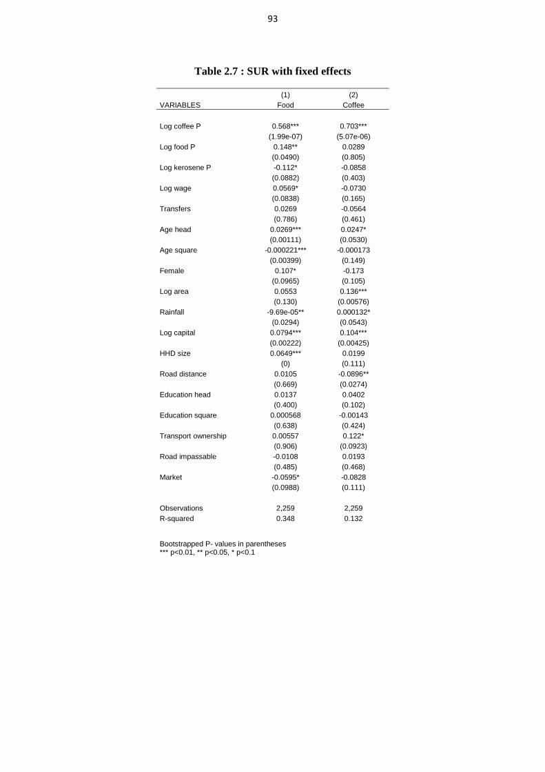
93

Table 2.7 : SUR with fixed effects

(1) (2) VARIABLES Food Coffee

Log coffee P 0.568*** 0.703***

(1.99e-07) (5.07e-06) Log food P 0.148** 0.0289

(0.0490) (0.805) Log kerosene P -0.112* -0.0858

(0.0882) (0.403) Log wage 0.0569* -0.0730

(0.0838) (0.165) Transfers 0.0269 -0.0564

(0.786) (0.461) Age head 0.0269*** 0.0247*

(0.00111) (0.0530) Age square -0.000221*** -0.000173

(0.00399) (0.149) Female 0.107* -0.173

(0.0965) (0.105) Log area 0.0553 0.136***

(0.130) (0.00576) Rainfall -9.69e-05** 0.000132*

(0.0294) (0.0543) Log capital 0.0794*** 0.104***

(0.00222) (0.00425) HHD size 0.0649*** 0.0199

(0) (0.111) Road distance 0.0105 -0.0896**

(0.669) (0.0274) Education head 0.0137 0.0402

(0.400) (0.102) Education square 0.000568 -0.00143

(0.638) (0.424) Transport ownership 0.00557 0.122*

(0.906) (0.0923) Road impassable -0.0108 0.0193

(0.485) (0.468) Market -0.0595* -0.0828

(0.0988) (0.111)

Observations 2,259 2,259 R-squared 0.348 0.132

Bootstrapped P- values in parentheses *** p<0.01, ** p<0.05, * p<0.1

94

Evolution of supply response

An interesting feature of the data is the long term longitudinal dimension which permits

analyzing how households’ behavior has changed from the first round of the survey in

91/93 to the second one in 2004.

In table 2.8 we show the results of the estimation of the supply functions for coffee and

food interacting respectively coffee and food price with the 2004 year dummy. The

results show that households are more responsive to prices in 2004 but only for food the

interaction term is statistically significant.

This result, although not conclusive, seems to give some credit to an increase in price

responsiveness over the time frame considered. Given the extensive reforms that have

been introduced in Tanzania in that very same period it would be interesting to explore

if there are links between the increased price responsiveness and the reforms in the

agricultural sector.

The problem we face in establishing any link is that during the nineties Tanzania went

through an extensive structural adjustment programme which involved changes in

almost all economic sectors and it is thus very difficult to disentangle the effect of

specific reforms from the overall adjustment. Also, changes in how supply responds to

prices can be due to technological changes which happen independently from any policy

action.

95

Table 2.8 : Evolution of supply response: FE with interaction term

(1) (2) VARIABLES Coffee Food Log food P 0.0170 -0.0322

(0.908) (0.683) Log food P*year04 0.374*

(0.0535) Log coffee P 0.682*** 0.401***

(0.000426) (0.000446) Log coffee P*year04 0.498

(0.121) Log kerosene P -0.101 -0.209***

(0.408) (0.00150) Log wage -0.0801 0.106***

(0.192) (0.00105) Transfers -0.0695* -0.00118

(0.0536) (0.984) Age head 0.0343** 0.0227***

(0.0451) (0.00615) Age square -0.000263* -0.000193**

(0.0880) (0.0110) Female -0.200 0.0201

(0.129) (0.765) Log area 0.109* 0.0912**

(0.0688) (0.0118) Rainfall 0.000167* -7.23e-05

(0.0566) (0.106) Log capital 0.185*** 0.0853***

(0.000464) (0.00104) HHD size 0.0269* 0.0810***

(0.0518) (0) Road distance -0.122** 0.0124

(0.0487) (0.528) Education head 0.0370 -0.00184

(0.218) (0.910) Education square -0.000903 0.00115

(0.660) (0.299) Transport ownership 0.125 0.0414

(0.180) (0.416) Road impassable 0.0384 -0.0162

(0.257) (0.305) Market -0.0884 -0.0570*

(0.168) (0.0983)

Observations 2,285 3,471 R-squared 0.149 0.302 Number of hhd 607 732 F 12.44 45.59 r2_w 0.149 0.302 r2_b 0.220 0.374 r2_o 0.210 0.336 Robust pval in parentheses *** p<0.01, ** p<0.05, * p<0.1

96

Testing the difference in supply response

In this section we test empirically the proposition that households facing full

functioning markets are more responsive to price changes for cash crops. In particular,

we analyzed in the theoretical section the own price elasticity of cash crops for

households which have a perfectly functioning market for food crops and compared this

to the one of households lacking access to the food market. The theoretical result shows

that under certain expectations about key measures as the income elasticity of

consumption and the cross elasticity of supply, the latter should be lower. However, we

pointed out that different results on these measures, however unexpected they can be,

can also reverse this result. In their study, de Janvry, Fafchamps and Sadoulet (1991)

use a simulation technique to test this proposition and find that households with missing

markets are actually less responsive to changes in the cash crop price.

We test this result on our sample of Tanzanian households comparing the supply

response of coffee for households that take part in the market for bananas, the main

staple food produced and consumed in the region, and households that instead are self-

sufficient.

In doing this comparison we need to take into account the potential selection bias

introduced by restricting the sample to participant in the bananas market and self-

sufficient. Given that we are using a panel dataset and the Heckman procedure is not

readily extensible to this case, we adopt instead the methodology proposed by

Wooldridge (1995) to test for selectivity in panel datasets. The methodology consists in

estimating the first stage probit equation by pooled probit and then using the inverse

mills ratio in the quantity equation. A standard t-test for the significance of the inverse

97

mills ratio is a valid test for selectivity even if this procedure is not valid to correct for

selectivity.

To reinforce the identification of the model we use three variables as proxy for fixed

transaction costs that affect the participation in the food market but not the volume

decision, these are the population density of the community were the household resides,

a dummy for the ethnic group of the head of the household (taking value of one if the

head pertains to the main ethnic group) and a dummy for the presence in the household

of a radio or a TV or a telephone. These variables should capture the degree of

information and network possibilities the household has and thus the degree of fixed

transaction costs as discussed also in Heltberg and Tarp (2002).

Results of the test are presented in table 2.9. The first column shows results for the

pooled probit where the dependent variable takes value of one if the household is self-

sufficient in the banana market and zero otherwise. The second column estimates the

coffee supply function for banana self-sufficient households as a standard fixed effects

adding the inverse mills ratio from the first step as a covariate. This is not statistically

significant which implies that, once controlling for the fixed effects, there is no

selectivity issue and the equation can be estimated as a normal fixed effects on the sub-

sample.

Table 2.10 reports estimation of coffee supply for the entire sample of households

producing coffee and bananas in the first column and then for the sub-sample of banana

self-sufficient households in the second column and for the other household who

participate to the banana market in the third column. The results show no substantive

difference in price responsiveness between the two groups which is in contrast with the

98

common belief that households who face missing food markets are less responsive on

the cash crop market.

There are two main reasons why these estimates can be biased. First, the instruments

used to identify the inverse mills ratio when testing for selectivity might be

inappropriate leading to a false rejection of the hypothesis of the presence selection bias.

Of the instruments used only population density is statistically significant and there are

reasons to think that this variable might not be orthogonal to the supply decision.

The second reason relates to the fact that multiple market imperfections are possible in

particular on the labour and credit market and this can interact with imperfections on the

food market confounding the estimates. Accounting for multiple market imperfections

is infeasible with small datasets like the one we are using.

99

Table 2.9 : Wooldridge test for selectivity

(Probit) (Fixed Effects)

VARIABLES

Self-sufficient bananas

Coffee production

Log coffee P -0.629*** 1.083

(0.000503) (0.151) Log food P -0.0417 0.232

(0.782) (0.522) Log kerosene P -0.00650 0.0178

(0.960) (0.952) Log wage 0.141** -0.437**

(0.0280) (0.0498) Transfers -0.151 0.226

(0.269) (0.251) Age head -0.00545 0.0148

(0.574) (0.732) Age square 9.51e-05 0.000272

(0.300) (0.486) Female -0.0527 0.117

(0.489) (0.735) Log area -0.0701 0.123

(0.304) (0.483) Rainfall 0.000184*** 0.000364

(0.00320) (0.219) Log capital 0.0741 0.0128

(0.141) (0.944) HHD size 0.0176 0.0209

(0.103) (0.624) Road distance -0.0285 -0.291***

(0.528) (0.00659) Education head 0.0199 0.00801

(0.380) (0.930) Education square -0.00387** 0.00410

(0.0399) (0.625) Transport ownership 0.0477 0.297

(0.481) (0.184) Road impassable 0.0579*** -0.0371

(0.000300) (0.685) Market -0.0407 0.0340

(0.551) (0.832) Density -0.000179**

(0.0103) Main ethnic group -0.0951

(0.170) Tv radio phone ownership 0.0209

(0.758) (0.0109)

Inverse Mills Ratio

-0.587

(0.682)

Constant 1.428 (0.132)

Observations 2,251 679 r2_p 0.0453

Number of hhd 363 F 6.118

r2_w 0.213 r2_b 0.104 r2_o 0.0982

Robust pvalues in parentheses *** p<0.01, ** p<0.05, * p<0.1

100

Table 2.10 : Separate FE estimations

(3) (4) (5) VARIABLES Overall Autarkic no-autarky

Log coffee P 0.821*** 0.859* 0.850***

(1.13e-05) (0.0679) (0.000366) Log food P 0.0682 0.197 -0.117

(0.645) (0.573) (0.540) Log kerosene P -0.120 0.00747 -0.117

(0.335) (0.979) (0.457) Log wage -0.0822 -0.381** 0.0314

(0.182) (0.0155) (0.684) Transfers -0.0376 0.159 -0.0464

(0.327) (0.235) (0.345) Age head 0.0319* 0.0113 0.0361*

(0.0688) (0.787) (0.0830) Age square -0.000227 0.000319 -0.000310*

(0.150) (0.391) (0.0970) Female -0.187 0.105 -0.287*

(0.169) (0.763) (0.0820) Log area 0.118* 0.0918 0.0683

(0.0522) (0.555) (0.340) Rainfall 0.000169* 0.000458** 0.000148

(0.0581) (0.0233) (0.194) Log capital 0.164*** 0.0481 0.153***

(0.00170) (0.751) (0.00888) HHD size 0.0279** 0.0275 0.0405**

(0.0471) (0.494) (0.0191) Road distance -0.127** -0.302*** -0.0438

(0.0431) (0.00432) (0.527) Education head 0.0372 0.0148 0.0629*

(0.220) (0.865) (0.0748) Education square -0.000953 0.00265 -0.00436**

(0.645) (0.714) (0.0483) Transport ownership 0.120 0.314 0.282**

(0.212) (0.151) (0.0136) Road impassable 0.00827 -0.0164 -0.00640

(0.823) (0.824) (0.885) Market -0.0860 0.00682 -0.177**

(0.188) (0.963) (0.0355)

Observations 2,251 679 1,572 Number of hhd 604 363 556

F 12.32 6.514 9.938 r2_w 0.147 0.212 0.174 r2_b 0.222 0.0999 0.226 r2_o 0.210 0.0942 0.204

Robust pval in parentheses *** p<0.01, ** p<0.05, * p<0.1

101

2.5 CONCLUSIONS

In this paper we estimated the supply response for cash and food crops for a sample of

farmers in the Kagera region of Tanzania using a long term panel dataset of households

in the region. The use of this data permits to control for households unobserved time

invariant characteristics and at the same time to analyze the impact of some variables of

interest which are quasi-fixed in the short term.

We find a positive own price supply elasticity for coffee while food supply is found to

be unresponsive to prices. We investigate the impact of transaction costs on production

and find that households more distant from a road produce less coffee. One kilometer of

additional distance reduces supply by 12%.

We find limited evidence that farmers are becoming more responsive to prices but

further research is needed to understand better the drivers of this evolution. We also find

no evidence that households facing market imperfections on the food market are less

responsive to prices for the cash crop. An overall test for separability rejects the

separability assumption.

102

Chapter 3

Supply response, market participation and transaction costs in food markets: evidence from a Tanzanian panel

3.1 Introduction

This chapter analyses the role barriers to trade in the form of high transaction costs have

on market participation and supply response in rural food markets in developing

countries.

Exploiting the availability of a long term panel dataset we develop an error components

switching regression model that takes into account individual unobserved heterogeneity.

The switching regression model endogenizes the three possible households’ choices of

being a food buyer, seller or self-sufficient and shows that measures of transaction costs

are both economically and statistically significant in explaining an increase in food

domestic production for buyers and a reduction for sellers. This implies a reduction in

the role of market exchange and a lower degree of specialization that would otherwise

arise in absence of transaction costs. The results also show the importance of

households’ heterogeneous market participation for the estimation of supply response.

High transaction costs have been considered an important feature characterizing the

functioning of rural markets in developing countries. A general definition of transaction

103

costs identifies them as all those costs that agents have to incur in order to conclude a

market transaction beyond the price of the good or service which are the immediate

object of the transaction.

The literature on the argument (Goetz 1992, Heltberg and Tarp 2002, Key et al. 2000)

has usually distinguished between two different types of transaction costs: proportional

transaction costs (PTC) and fixed transaction costs (FTC). The former vary in function

of the quantity traded and the latter instead are a lump sum representing the one off cost

of entering a market irrespective of the quantity traded.

PTCs include the costs of transferring the good traded such as its transport and the time

spent in between to reach the market. FTCs include the costs of: a) searching for a

market or a trading partner; b) negotiating and bargaining; c) screening, enforcing and

supervising contracts.

The main challenge we face when analyzing the impact of transaction costs is that they

are usually not observed and measured directly in most surveys. What we often observe

are some factors which are thought to affect them. For example, FTCs such as

searching, screening and so on are very difficult to quantify directly but we can instead

observe other variables which indicate agents’ degree of information and network

relationship available which are expected to determine their FTCs.

The effect that transaction costs have on farmers is twofold: on the one side they

directly affect the effective price received by sellers and paid by buyers and thus the

quantities exchanged. On the other side, transaction costs also generates heterogeneity

in the way households relate to markets and can potentially explain why some farmers

104

decide to take part to the market exchange while others remain self-sufficient. In

particular fixed transaction costs can be seen as barrier to trade which need to be

overcame if the farmer has to take part to the market.

The implication for the estimation of agricultural supply response is that both the

heterogeneity in market participation and the role of non-price factors have to be taken

into account to obtain correct estimates of supply response. In particular, accounting for

the heterogeneity in market participation implies the estimation of separate supply

functions for each market regime as they are likely to behave differently and to respond

to different incentives.

In the following sections after a review of the literature on supply response and market

participation we review the theoretical framework which incorporates transaction costs,

heterogeneity in market participation and supply response. Then we account for the

problem we have to face when using a panel data for this analysis and our strategy to

address it. We then report the results of the empirical analysis and finally draw some

conclusions.

3.2 Literature review

Several studies have addressed under a wide spectrum of angles and methodologies the

role that transport costs, infrastructure, isolation and transaction costs play in shaping

economic decisions and the process of economic development. In recent years a number

of studies have dedicated an increasing amount of attention to the role of rural

infrastructure in developing countries identifying channels reasons through which rural

105

infrastructure and transaction costs can influence agricultural production, income and

poverty in developing countries’ rural areas.

Transportation and transaction costs can affect directly agricultural productivity and

output. Productivity can be affected through input adoption as the price of imported

inputs rises the higher are transportation costs but also through increased price volatility

or differing specialization patterns and crop mix. Stifel and Minten (2008) present

evidence that transportation costs reduce rice yields and input use in Madagascar.

Dorosh et al. (2010) also show a significant effect of road infrastructure on agricultural

output and input adoption using a more aggregated cross-sectional spatial approach for

Sub-Saharan Africa.

One factor explaining the inverse relationship between productivity and transportation

costs runs through the effect they have on the level of specialization and choice of the

crop mix. The evidence on the link between transaction costs and specialization is

mixed. Qin and Zhang (2011) directly link the Herfindal specialization index to road

access in a Chinese rural province and find a higher degree of specialization among

better connected households. Stifel et al (2003) found for a sample of households in

Madagascar a lower level of concentration of agricultural production in more isolated

areas and a shift towards staple food production at the expenses of more valuable crops.

On the other hand, Gibson and Rozelle (2003) find that increased isolation reduces the

number of income generation activities pursued by households and thus increases

specialization of income sources. Omamo (1998) uses simulation techniques to show

that households facing higher transaction costs tend to alter the crop mix and increase

the share of food crops at the expenses of cash crops.

106

A somewhat different but interrelated aspect implied by high transaction costs concerns

the impact they have on the degree of commercialization and on farmers’ market

participation decisions. The literature on market participation and transaction costs has

shown that high transaction costs can drive households out of the market as an optimal

strategy to avoid high fixed and proportional transaction costs (De Janvry et al. 1991).

The main implication of this finding is that transaction costs will generate heterogeneity

in how households relate to the market as some will optimally choose not to take part to

market transactions. This in turn might imply heterogeneous behavior that needs to be

taken into account in empirical applications and requires an appropriate econometric

strategy.

Goetz (1992) in his pioneer study of Senegalese grain market analyses the marketing

behavior of buyers and sellers respectively. He models the discrete market participation

decision of buyers and sellers and then estimates separate market surplus equations

accounting for selectivity into the corresponding regime. The evidence is not totally

conclusive but it does show that information is a significant driver of market

participation decisions. The drawback of this study is that it looks only at how fixed

transaction costs influence households’ decision to enter the market while not allowing

for the role of transaction costs in influencing the quantity transacted.

With a similar approach, Heltberg and Tarp (2002) in their study of supply response in

Mozambique model selling farmers’ marketing behavior. They found evidence that

ownership of a means of transport and proximity to a railway increases both the

likelihood of entering the market as a seller and the quantity sold. The break-down of

the marginal effect into the entry/exit and quantity components shows that the first

107

effect is substantially larger. Implying that promotion of market access can solicit a

greater volume of additional supply from peasants entering the market for the first time

than for existing participants. The study suffers from two shortcomings. First, they use

cross-sectional data and are not able to identify any price effect which limits their ability

to compare the effectiveness of price versus non-price factors in increasing market

participation and sales. Second, the proxy used for fixed transaction costs as population

density and information dummy are not statistically significant casting some doubts on

the identification of the model.

Key, Sadoulet and de Janvry (2000) follow a different approach in their study of

Mexican farmers’ participation in the maize market. They estimate a structural model of

market participation and supply decisions taking into account the distinct role of

proportional and fixed transaction costs. They jointly estimate the supply functions and

the production thresholds using a censoring model with unobserved censoring

thresholds. Here the focus is not on marketing behavior but on production behavior

given the heterogeneity in market participation. They found that both proportional and

fixed transaction costs do matter for market entry and output decisions.

Bellemare and Barrett (2006) look at the pastoralists’ participation in livestock markets

in Ethiopia and Kenya and estimate the determinants of marketing surplus for the

different regimes of net-buyers, net-sellers and self-sufficient. Ouma et al. (2010)

analyze smallholders’ participation in banana markets in Central Africa adopting an

approach very similar to the one presented by Goetz (1992) showing that farmers

located one hour further from the nearest urban market reduce the transacted quantities

by 17% for sellers and 12% for buyers. Alene et al. (2008) present a study of maize

108

supply and fertilizer demand in Kenya and find that farmers located far from the market

reduce transacted quantities by 62%.

Some of the above studies look at the market surplus as opposed to supply. Their aim in

that case is to analyze marketing behavior estimating the determinants of the quantities

bought or/and sold while controlling for the endogenous selection into the respective

market participation regime. Other studies look instead at the production side only and

estimate the determinants of quantity produced controlling for regime selection.

Other studies have focused more on the role of transaction costs in the labour and land

market. Carter and Yao (2002) estimates regime specific equations for the households’

labor intensity taking into account their participation regime in the land rental market.

The transaction cost in their study is a measure of legal limitations which encumber

transactions in the land market in China. They use an ordered probit as selection

equation and estimate both selection and outcome equations using simulated maximum

likelihood. They use a panel dataset of Chinese households and make use of a correction

to control for households’ fixed effects. Sadoulet, de Janvry and Benjamin (1998)

model households labor intensity distinguishing across regimes of participation in the

labor market for a sample of Mexican households. They apply a two-step procedure à la

Heckman where however the first step selection equation is an ordered probit.

The above studies while all pertaining to the same stream of literature on market

participation and transaction costs differ in some important aspects. The econometric

strategy varies. Some studies make use of the ordered structure of the regime choice

while others do not. As we will show in the theoretical model in the next section an

109

ordered structure for the market participation decision is in principle preferable as it

exploits the ordered structure of the relationship, but it also complicates the estimation.

The type of data used is generally cross-sections, only few studies make use of

longitudinal data in this literature and when they do, apart from Carter and Yao (2002),

they treat them as cross-sections even if the econometric literature has established the

potentially serious biases this procedure involves when individual unobserved

heterogeneity is present. The availability of longitudinal data potentially also opens up

the possibility to explore the dynamic pattern of market participation. The main aim of

this paper is to address these shortcomings and use the longitudinal data at hand to

incorporate unobserved heterogeneity into the analysis.

3.3 Theoretical framework

Before introducing a more formal treatment of the implication of transaction costs for

market participation and the estimation of the supply function it will be useful to look at

the intuition behind just comparing the scenarios in presence and absence of transaction

costs.

Consider a farm household which both produces and consumes food. The household

will be characterized by a demand and a supply function (figure 3.1). In absence of

transaction costs the household is a net-seller if the market price (pm) is higher than the

shadow price (p*) defined as the price that would equate demand and supply of the

household. In a similar way the household would be a net-buyer if the shadow price is

higher than the market price (p’m). The passage from being a net-buyer to being a net

110

seller is a continuous one and only in the limited case when the shadow price equals

exactly the market price non-participation in the market would be a utility maximizing

choice.

Figure 3.1 Net-sellers and net-buyers

P

D m>0 S

pm

p*

p’m

m<0

Q

Thus, in absence of transaction costs households face a single price for buying and

selling and all will take part in the market either as buyers or sellers. The set of

autarchic households should tend towards emptiness.

The introduction of proportional transaction costs, as said, would increase the effective

price paid by buyers while reducing the effective price received by sellers and thus

generates a price band between the two prices. As in the case where there are no

transaction costs, the choice of the regime of market participation is based on comparing

the utility obtained in the different regimes for a particular commodity. The difference is

that the presence of a price band is likely to generate a set of households for which

utility is maximized by being self-sufficient and not taking part to the market exchange.

111

A third regime, autarky or self-sufficiency, is now possible and market participation

becomes a discrete choice for effect of the price band generated by transaction costs.

The utility obtained in different regimes and thus the decision on whether to take part in

the market depends on a comparison between the shadow price of those goods with the

buying and selling market prices. If the shadow price is higher than the buying price

then the household will maximize its utility level by being a net-buyer. If the household

shadow price is below the market selling price then the household will be better off as a

net-seller. Finally, if the shadow price falls within the band non-participation is the

utility maximizing strategy for the household. Figure 3.2 represents three different

hypothetical households differing only in term of the supply (Sa, Sb and Sc). The

different point where supply crosses demand determines household’s market position.

Figure 3.2 Households’ market position

P Sa

Sb

D Sc

Pb

Ps

Q

The role of transaction costs can be analyzed in a formal model which endogenises

market participation decisions. The model presented below follows closely the one

112

proposed by Key et al (2000), one of the most complete expositions of the role of

transaction costs in rural food markets. Consider a utility maximizing household which

consumes a set of goods ci and produces qi agricultural products. To simplify notation

let’s define mi as the marketed surplus for good i and express the cash constraint in

terms of marketed surplus taking into account transaction costs. Market prices are

corrected for proportional transaction costs which add to the market price in case of

goods purchased ( 0im < ) and reduce the effective sale price ( 0im > ). Transaction costs

(τ) are differentiated between proportional ( )piτ and fixed ( )fiτ transaction costs and

between buyers ( )bτ and sellers ( )sτ . They are not directly observed but some factors

affecting them ( ft ) are observed. zc and zp are respectively households’ consumption

and production shifters. The household’s problem is to choose quantities of

consumption goods in order to maximize utility subject to a set of constraints:

1

max ( ; )

s.t

( ; ) 0

0

( ( )) ( ( )) ( ) ( ) 0

ci

c

pi

i i i

Nm s s s m b b b s s s b b b

pi t i pi t i i fi t i fi t ii

U c z

g q z

q m c

p f p f m f f Eτ δ τ δ τ δ τ δ=

=− − =

− + + − − + = ∑

The first constraint is a standard well-behaved production function. The second is a

resource constraint imposing that quantities consumed are equal to quantities produced

deducted (added) sales (purchases). The third constraint is a cash constraint imposing

that expenditures need to be equal to revenues from the sale of farm products plus the

exogenous income E taking into account proportional and fixed transaction costs ( jiδ

113

takes value of one if the household is class j and zero otherwise). The lagrangian for this

problem is:

1

( ; )

[ ( ( )) ( ( )) ( ) ( ) ]

( ; ) ( )

ci

Nm s s s m b b b s s s b b b

pi t i pi t i i fi t i fi t ii

pi i i i

L U c z

p f p f m f f E

g q z q m c

λ τ δ τ δ τ δ τ δ

φ η=

=

+ − + + − − +

+ + − −

∑

Given the presence of fixed transaction costs which generates discontinuities in the

Lagrangean function Key et al. (2000) show how the solution can be decomposed into

two steps, first finding the optimal solution conditional on the market participation

regime and then choosing the market participation regime which maximizes utility.

The first order conditions for consumption goods, outputs and traded goods assuming

interior solutions are respectively:

0

0

( ( )) ( ( )) 0

i

i

m s s s m b b bpi t i pi t i

U

c

g

q

p f p f

δ ηδ

δφ ηδ

λ τ δ τ δ η

− =

+ =

− + + − =

We can define the decision price as:

*i

if 0, seller

if 0, buyer

p if 0, self-sufficient

m si pi i

m bi i pi i

i

p m

p p m

m

τ

τηλ

− >= + < = =

114

The problem is now to choose the utility maximizing regime by comparing utilities

under different regimes. Using the above defined decision price we can define the

maximum utility attained in each regime using the same indirect utility function

( , , )ciV p y z . Define 0( )iy p as the household income before incurring any fixed

transaction costs:

01

( )N

i i ii

y p p q E=

= +∑

Then the utility levels for different regimes can be written as:

0

0

* *0

( , ( ) , ) if seller

( , ( ) , ) if buyer

( , ( ), ) if autarkic

s m s m s s cp p f

b m b m b b cp p f

a c

V V p y p z

V V p y p z

V V p y p z

τ τ τ

τ τ τ

= − − −

= + + −

=

These expressions show that in absence of fixed transaction costs the household would

be indifferent between selling and being self-sufficient if * m spp p τ= − . From the FOC it

can be shown that utility is increasing in the decision price for sellers and decreasing in

the decision price for buyers. Thus, if *m spp pτ− > a household facing no fixed

transaction costs would be better off selling. In a similar way, the household will be

indifferent between buying and being self-sufficient if * m bpp p τ= + and it would be

better-off buying on the market if *m bpp pτ+ < .

115

Figure 3.3 Indirect utility function

pm Va D

Vs

*m s

pp p τ= + C

*m b

pp p τ= − B

Vb

A

V

116

Figure 3.3 shows the indirect utility function V as a function of the market price. The

vertical line shows the utility attainable by autarkic households which is independent of

the market price. At point C the household will be indifferent between selling and being

autarkic and for prices above C it will be a seller with utility increasing with price. At

point B the household will be indifferent between buying and being autarkic and for

prices below B it will be better-off buying with utility decreasing with the price. If the

market price is between B and C the household will be better-off staying in autarky. The

optimal market participation strategy is ABCD.

The implication of the introduction of fixed transaction costs as well as the proportional

ones can be shown looking at the fact that fixed transaction costs lower household

income and thus utility for each level of price. This will shift the utility curves to the left

as shown in figure 3.4. Fixed transaction costs will thus discourage households from

entering the market until the price is sufficiently high (low) to cover fixed transaction

costs for sellers (buyers), points E and F in figure 3.4.

Figure 3.4 Fixed transaction costs

Pm D’

E

F A’

V

117

However, fixed transaction costs do not enter household’s supply curve because only

the marginal return to production affects production decisions. The first implication of

this finding is that once entering the market either as a buyer or seller there will be a

discrete jump in the quantity produced as the decision price will change discretely. The

supply function derived has three distinct regimes for different price levels and is shown

in figure 3.5. The vertical part of the supply function corresponds to the autarkic regime

which is unresponsive to prices. The lower segment AF is the buying region and finally

the upper segment ED corresponds to the selling region. The discrete change in the

quantities produced when entering the market either as buyer or seller can also be seen

in figure 3.5 at the points Qs and Qb. These two quantities are the quantity thresholds

below which it is not optimal for the household to enter the market.

The second important implication of this distinct role of fixed transaction costs is that it

gives a way of econometrically identifying the parameters of both the market

participation and volume decisions.

Figure 3.5 Supply function

Pm D

C E

F B

A

Qb Qs Q

118

The above analysis has several implications for the estimation of supply response.

First, we need to take into account the unresponsiveness of autarchic households.

Unless this is accounted for it is likely that pooled estimates of the true underlying

supply response will be downward biased.

Pooled estimates of the supply response would in principle provide an unbiased

estimate of the unconditional supply response. They present an appropriately weighted

average of the positive supply responses of households taking part to the market and the

null supply response of self-sufficient households. However, pooled estimates cannot

provide an unbiased estimate of the underlying supply elasticity conditional to the

market participation regime which is an important piece of information if we want to

evaluate the impact of different policies on different subsamples. Moreover, pooled

estimates cannot take into account the fact that households could potentially switch

regime following a price change changing in this way the weights of the simple

elasticities.

Second, changes in prices and other non-price factors which affect market participation

decisions should be accounted for in the estimation of the overall supply response.

Third, transaction costs have a different impact on buyers and sellers and estimation of

regime specific supply functions can help identify and test the effective importance of

transaction costs on production behavior. For a seller an increase in transaction costs is

expected to have a negative effect on production. For a buyer instead an increase in

transaction costs is expected to have a positive impact on production.

119

In the following sections, after discussing the econometric challenges we face when

using longitudinal data in this context, we will try to estimate empirically this model

and analyze in a coherent framework market participation and supply decisions.

3.4 Discrete choice models for longitudinal panel data

The analysis of how transaction costs affect the market participation decision and how

this decision in turn affects supply response implies the need for models able to

consider simultaneously the discrete choice on market participation and the continuous

one regarding output. The literature on discrete choice models and selection models is

very extensive and several different techniques have been developed14. The extension of

these techniques to longitudinal panel data is however not completely straightforward

and developments in this area for panel data have been slower. This section analyses the

econometric problems related to applying discrete choice modeling to panel data.

The easiest way to show the problems that discrete choice models present in a panel

data context is to analyze the basic probit model which serves as the basis for other

more complex extensions as ordered and selection models.

The distinction between random and fixed effects normally made in a linear context also

applies to discrete choice models. The key difference is that a fixed effect estimator

does not pose any restriction to the correlation structure of the individual heterogeneity

and the set of explanatory variables while the random effect model assumes that there is

no correlation between the individual heterogeneity and the other covariates. This

14 See Greene (2008) for a review.

120

assumption, needed for consistency of the random effect model, is an important

drawback in most applications.

There are no particular problems in extending the random effect specification to discrete

choice models like the probit model. However, the same is unfortunately not true for the

fixed effect specification which has been shown in different studies to be an inconsistent

estimator of the underlying parameters. The main aspect to notice here is that, as

opposed to linear panel models, here it is not possible to find a suitable transformation

(like the within transformation) that removes the individual effects. The only alternative

is to include the full set of dummies and estimate what Greene (2001) calls a brute force

estimator. This option is feasible computationally (although quite intensive) but suffers

from the incidental parameter problem. This problem arises because a sufficient statistic

able to sweep out the fixed effects is not available and slope parameters have to be

estimated as a function of the fixed effects. Estimates of the fixed effects are

inconsistent in small t panels (they do not converge asymptotically to the true parameter

if n increases but t doesn’t) and this means that also the slope parameters would be

inconsistent.

In the absence of a fixed effect estimator the model can be estimated as a random effects

model. The additional assumption needed for consistency of the random effects is that

the individual specific effects are normally distributed with zero mean and constant

variance:

2 [0, ]i uu N σ∼

The difficulties in estimating discrete choice models for panel data also carry over to

models of sample selection which are further complicated by the fact that the common

121

two-step Hackman procedure15 often used in cross-sectional analysis to control for

selectivity is not readily available for panel data. The sample selection bias may arise

because the subsample of households not participating in the food market is non-

randomly selected.

A general model with selection can be formalized as follow:

*

*

*

*

1 if 0; 0 otherwise

y

i i i

i i i

i i i

i i i

y x

d z v

d d d

y d

β εγ

= +

= +

= > =

= ∗

d* represents the selection equation while y is the outcome variable of primary interest.

The main problem in this setting is that it is likely in most applications that

unobservables affecting the selection decision are correlated with the unobservable in

the outcome equation:

( , ) 0i iE vε ≠

If that is the case the errors in the selection and outcome equations are likely to be

correlated. OLS over the sub-sample where 1id = would give biased and inconsistent

estimates for the correlation of x and ε introduced through the correlation of v and ε.

A common solution to the general selection problem is Heckman’s two-step estimation.

Consider a situation where in the model above specified ε and v have a bivariate normal

distribution with covariance vεσ .

2 2, (0,0; , ; )v vv BVN ε εε σ σ σ∼

15

Heckman (1979).

122

We are interested in the determinants of y for a selected sample of households where d*

exceeds zero and thus 1id = . Defining φ and Φ as respectively the normal density and

cumulative distributions we have:

*

2

2

[ | 1] [ | 0]

[ | ]

[ | ]

[ | ]

( / )

1 ( / )

i i i i

i i i

i i i i

vi i i i

v

v vi v

v v

E y d E y d

E y v z

x E v z

x E v v z

zx

z

ε

ε

γβ ε γ

σβ γσσ φ γ σβ σσ γ σ

= = >= > −= + > −

= + > −

−= +− Φ −

( / )

( / )v

iv

zx

zεφ γ σβ ρσ

γ σ= +

Φ

The model then becomes:

[ | 1] [ | 1] ( )i i i i i i i iy d E y d u x z uλβ β λ γ= = = + = + +

OLS estimation on the selected sample without correction leads to biased estimates

because of the omission of the relevant term λ, the inverse Mills ratio.

An important issue concerning the Heckman procedure is the identification strategy. In

principle the model can be identified through non-linearities in the probit model.

However, this strategy can result in a weak identification with inflated second step

standard errors and unreliable estimates of the coefficients (Vella 1998). To avoid these

problems additional variables included in the selection equation but excluded from the

outcome equation should be found in order to help identification.

123

The extension of the selection model to a panel data setting is not straightforward.

Rewriting the above selection model to take into account the longitudinal nature of the

data we obtain:

*

*

*

*

1 if 0; 0 otherwise

y

it it i it

it it i it

it it it

it it it

y x

d z v

d d d

y d

β µ εγ α

= + +

= + +

= > =

= ∗

In this case the two error components, individual heterogeneity (μi) and idiosyncratic

error (εit), are assumed to be correlated with the same component in the other equation

generating a problem of selection.

Looking at the fixed effect estimator we can derive the conditions for its consistency

following Wooldridge (2010) and Vella (1998). Applying the within transformation to

the data we obtain the fixed effect estimator of β as follow:

1

1 ' 1 '

1 1 1 1

1

1 ' 1 '

1 1 1 1

ˆN T N T

it it it it it it

i t i t

N T N T

it it it it it it

i t i t

N d x x N d x y

N d x x N d x

β

β ε

−

− −

= = = =

−

− −

= = = =

=

= +

∑∑ ∑∑

∑∑ ∑∑

ɺɺ ɺɺ ɺɺ ɺɺ

ɺɺ ɺɺ ɺɺ

Where

1 1

1 1 1

T T T

it it i it it it it i it it i it

t t t

x x T d x y y T d y T d− −

= = =

= − = − =∑ ∑ ∑ɺɺ ɺɺ

Consistency of the fixed effect model thus requires '( ) 0itit itE d x ε =ɺɺ . This in turn requires

( | , , ) 0it it it iE x dε µ =

124

which imposes no restrictions on the relationship between id and ( , )i ix µ . The only

restriction is that the idiosyncratic error is independent of the selection indicator which

in turn requires no correlation between ε and v.

Thus, consistency of the fixed effect estimator would be guaranteed if the selection

operates only through the individual specific effect iα . The same result does not apply

for the random effect estimator which instead is inconsistent also if the selection

operates through the individual effect. In principle, in situations in which we are

confident that the selection operates only through the individual effect we could

estimate a fixed effect model neglecting the selection issue. However, these conditions

are not always met and it is important to at least test for selection in any case.

However, extending the Heckman procedure to panel data presents several

complications that are not easy to address. The first of these is the inconsistency of the

fixed effects probit estimator for small t-dimension panels discussed above which brings

us far away from the use of fixed effects estimators.

A first idea would be to run a pooled probit for the selection equation, obtain the inverse

Mills ratio and estimate the outcome equation by fixed effects including the selection

correction. This method however does not produce consistent estimators either

(Wooldridge 2010).

A second option, adopted by Ridder (1990) and Nijman and Verbeek (1992) would be

to estimate the first step by random effects probit, obtain correction terms and then

estimate the second step by OLS with the correction terms added. This procedure

closely resembles the Heckman procedure but the correction terms have a different and

more complex form than the inverse Mills ratio.

125

Other models to correct for selectivity in panel data have been developed. In particular,

we will focus in our empirical application on a model proposed by Zabel (1992) which

departs from two-step procedures and proposes a Full Information Maximum

Likelihood (FIML) estimation. This significantly increases the computational burden of

the estimation but provides a coherent framework for the joint estimation of selection

and outcome equations.

In the next section we adapt Zabel’s model to the ordered nature of our problem to

analyze supply decision controlling for the market participation regime.

3.5 Supply response and market participation: A panel selectivity

model with an ordered probit selection rule

We adopt a Full Information Maximum Likelihood approach instead of the two step

procedure. The model was first proposed by Zabel (1992) in the context of a binary

probit selection rule and as an alternative to other two step procedure developed before.

As shown above, in our case an ordered selection rule would be more appropriate. The

main drawback of Zabel’s approach was its computational intensity but as noted in

Greene (2006) the development of simulation methods have to some extent made it

easier to estimate such models. Carter and Yao (2002) present one application of the

same family with an ordered probit selection rule.

We sort individuals (or households) into J+1 classes according to an ordered probit

selection rule:

126

* '

*0

*0 1

*1 2

*1

0 if - < d

1 if d

2 if d

.......

if < d

it it i it

it

it

it it

j it

d Z r u

d

J

γ

µµ µµ µ

µ −

= + +

∞ ≤

≤ ≤= ≤ ≤ < +∞

where *itd is a latent unobserved variable assumed to be dependent on a vector of

explanatory variables Z , a vector of unknown parameters γ, an individual specific

heterogeneity component ir assumed to be random and an idiosyncratic random term

itu . What we actually observe is the discrete variable itd which takes values from 0 to J

to distinguish the J+1 classes.

For each of the J+1 classes we observe an outcome variable:

' with 0,1,..,itj J itJ iJ itJ itY X v d Jβ ε= + + =

itjY is the outcome variable, at time t for household i belonging to class j and is a linear

function of a vector of explanatory variables itjX , an individual specific time invariant

random effect ijv and an idiosyncratic error term itjε .

Both the outcome and selection equations allow for the presence of individual random

effects. There are J+1 random effects in the outcome equations and an additional one in

the ordered probit equation for a total of J+2 random effects. The assumptions needed

for the random components and the idiosyncratic error are:

2

2

(0, )

(0, )

ij vj

itj j

v N

N ε

σ

ε σ

∼

∼

127

for the outcome equations and

2(0, )

(0,1)i r

it

r N

u N

σ∼

∼

for the ordered probit selection equation. The variance of u is normalized to unity for

identification purposes.

To simplify the estimation we assume the individual-specific error terms are

uncorrelated with each other, an assumption which could in principle be relaxed. Each

of the idiosyncratic error terms in the outcome equations εitj and the one in the selection

equation uit have instead correlation coefficient jρ . Thus, εitj and uit follow a bivariate

normal distribution:

2 22( , ) (0,0; ,1; )itj it j j ju N ε εε σ ρ σ∼

The likelihood for individual i has the following form:

( ) ( ) ( )1

2 2

( ) Pr( | )

1

1 1

i itj it itj

t

it i j itj j it i j itj jitj ij i ij i

j j jt

L f y d j y

Z r t Z r tt v r dv dr

ε

γ ρ µ γ ρ µφ φ φ

σ ρ ρ−

= × =

+ + − + + − = Φ − Φ − −

∏∏∫∫

Where '

itj j itj ijitj

j

y X vt

ε

βσ

− −= , ϕ is the standard normal density function and Φ is the

standard normal cumulative function. The derivation uses the fact that given the joint

distribution of 2 22( , ) (0,0; ,1; )itj it j j ju N ε εε σ ρ σ∼ the conditional distribution of u given εj

is:

128

2 2( | ) ( ;1 ) ( ;1 )j jit itj j j itj j

j

u N N tε

ρ εε ρ ρ ρ

σ− = −∼

Then the log-likelihood is ln ln ii

L L= ∑ .

The likelihood requires a double integration for any observation and is computationally

intensive. However, recent developments in simulation methods provide a way to

evaluate the above likelihood function. Simulation techniques are methods to

numerically approximate otherwise intractable integrals. There are various forms of

simulation used for different kind of problems16. In our case it is enough to notice that

the above integrals are expectations over the random individual effects:

[ ]1 2(.)[ (.) (.)] /r vE E φ σ Φ − Φ

and these expectations can be approximated with the average of a sufficient number of

draws from the standard normal distribution generating r i and vij.

Letting g=1,…,G count the draws of the simulation model, the above likelihood

function can then be approximated with the following simulated likelihood function:

( ) , , 1 , ,, 2 2

1

1 1

1 1

G

it i g j itj g j it i g j itj g jsi itj g

j j jg t

Z r t Z r tL t

G ε

γ ρ µ γ ρ µφ

σ ρ ρ−

=

+ + − + + − = Φ − Φ − −

∑∏

16 Examples of recent applications of simulation techniques are, among others, Hyslop (1999) on married women labour participation choices, Cappellari and Jenkis (2004) on movements in and out of poverty, Morris (2003) on educational choices, Razo-Garcia (2010) on exchange rate ragimes and financial account openness.

129

where '

,,

itj j itj ij gitj g

j

y X vt

ε

βσ

− −= . ,i gr and ,ij gv are random draws from the respective

normal distributions and G is the total number of draws taken from the distributions of v

and u. The variance of v and u is unknown and needs to be estimated within the model.

To generate the random draws we follow Train (2009)17 and use draws derived from

Halton sequences which improve accuracy with a reduced number of draws with respect

to pseudo-random number generators. This is due to the fact that draws derived from

Halton sequences increase the coverage of the domain of integration and induce a

negative correlation between the draws thus reducing the variance of the simulation.

The Halton method works by first defining a sequence by using a particular prime

number, P. The elements of the sequence are then obtained by an iterative process

comprising a series of successive rounds. In the first round, the unit interval is split into

P equal-width segments, and elements with values equal to the P–1 segment cut-points

are defined. In the second round, each segment created in the first round is further split

into P new segments. P-1 new elements are picked for each segment. In the next round,

each segment is split P ways again and the cycling continue for as long as one needs

sequence elements. As the number of rounds increases, the unit interval gets more and

more filled in by sequence elements.

The simulated likelihood is then maximized numerically with respect to the parameters

1 1, , , , , , ..j j vj r j jεβ γ σ σ σ ρ µ µ − . This method is called Maximum Simulated Likelihood

(MSL)18.

17 See Cappellari and Jenkins (2006) for a brief review of the different methods available to generate random draws for MSL and their relative advantages. Also, they develop the Stata routine mdraws used for this application to generate Halton sequences. 18 See Train (2009) and Gourieroux and Monfort (1993).

130

In our case the classes of market participation are three, in order: buyers, autarchic and

sellers.

(0.0)

* '

*0

*0 1

*1

0 if - < d if buyer

1 if d if autarchic

2 if < d if seller

it it i it

it

it it

it

d Z r u

d

γ

µµ µµ

= + +

∞ ≤

= ≤ ≤ < +∞

For each regime of market participation we observe food supply:

(0.0)

'

'

'

if 0

if 1

if 2

it

it

it

BB itB iB itB it

AA itA iA itA it

SS itS iS itS it

Y X v d

Y X v d

Y X v d

β ε

β ε

β ε

= + + = = + + =

= + + =

The likelihood of a household being respectively a buyer, autarchic and seller at time t

is then given by the above formulas and the full log-likelihood is obtained taking the

within-group product over time of the single observation likelihoods, integrating these

products over the random effects, taking logs and summing over groups we obtain the

full log-likelihood:

{ } { } { } ( ) ( )ln lnab sB A S

it it it iA i iA i

i t

L L L L v r dv drφ φ=∑ ∏∫∫

Where the exponents b, a and s take value of 1 if the household i at time t is

respectively a buyer, autarchic or seller and zero otherwise.

The simulated likelihood is derived as follow:

{ } { } { }1ln ln

b a ss s B s A s Sit it it

i g t

L L L LG

=∑ ∑∏

131

where the super-script s denotes simulated values. In our estimation we use 50 random

draws to approximate the likelihood function. Gourieroux and Monfort (1993) show

that with this method a moderate number of replications is enough to obtain a good

approximation of the likelihood function.

We develop a Stata routine to implement the above model using Maximum Simulated

Likelihood technique. Appendix 3 reports the Stata code.

3.6 Empirical Analysis

The KHDS dataset offers several interesting insights into the evolution of agriculture in

the region and the different behaviour of households pertaining to different food market

regimes. Table 3.1 shows some descriptive statistics on households’ production

structure for 1991 and 2004 decomposed by regime of market participation in the food

market.

The share of agricultural production in total expenditures, as already noted in chapter

one, drops quite dramatically during the period across all categories. Food net-buyers

are the group where agriculture accounts for the lower share of expenditures. Staple

food maintains a high and stable share of total production across all the three categories.

Yields have actually decreased during the period. While this might be due to the life-

cycle evolution of our sample or to contingent weather-related factors it is an indication

of a stagnant agricultural sector. Notably yields are on average lower for food net-

buyers in both years. An indirect confirmation of the stagnation of agriculture comes

from input use figures. The proportion of households applying fertilizers and pesticides,

132

if low in both periods, has actually dropped even more. Again, net-buyers show a lower

inputs adoption.

133

Table 3.1 : Descriptive statistics

1991

Net-buyers Autarky Net-seller Overall

Mean Sd Mean Sd Mean Sd Mean Sd

Yield (000') 90.0 141.7 93.5 135.6 120.3 275.9 102.9 207.5

Consumption pc (000'tsh) 189.1 125.3 150.1 94.3 195.9 139.8 187.2 129.0

Production shares

Food 0.71 0.19 0.67 0.2 0.7 0.17 0.7 0.18

Coffee 0.04 0.07 0.09 0.14 0.07 0.1 0.06 0.09

Vegetables 0.03 0.06 0.02 0.04 0.03 0.04 0.03 0.05

Other cash crops 0 0.03 0.01 0.06 0 0.03 0 0.03

Fruits 0.07 0.1 0.07 0.08 0.06 0.08 0.07 0.09

Other food 0.09 0.12 0.08 0.09 0.06 0.1 0.08 0.11

Other crops 0.06 0.09 0.07 0.09 0.07 0.08 0.07 0.09

Expenditure shares

Agricultural production 0.54 0.34 0.73 0.53 0.77 0.59 0.66 0.49

Sales 0.05 0.09 0.09 0.15 0.14 0.13 0.09 0.12

Purchases 0.57 0.2 0.43 0.18 0.49 0.17 0.52 0.19

Inputs

Land size (acre) 3.64 2.76 4.48 2.95 4.95 2.97 4.29 2.94

Hired labor (% hiring) 19 40 14 35 37 48 26 44

Fertilizer (% applying) 5 21 4 21 7 26 6 23

Pesticide (% applying) 8 27 9 28 19 39 13 33

Manure (% applying) 45 50 42 50 45 50 45 50

N 329 91 295 715

2004

Net-buyer Autarky Net seller Overall

Mean Sd Mean Sd Mean sd Mean Sd

Yield (000') 54.0 76.5 69.4 118.8 83.9 103.6 69.3 96.4

Consumption pc (000'tsh) 181.9 131.6 188.5 129.7 215.5 187.9 197.7 159.4

Production shares

Food 0.72 0.17 0.73 0.18 0.72 0.16 0.72 0.17

Coffee 0.03 0.06 0.03 0.07 0.05 0.08 0.04 0.07

Vegetables 0.02 0.06 0.02 0.05 0.02 0.04 0.02 0.05

Other cash crops 0 0.03 0 0 0 0.04 0 0.03

Fruits 0.05 0.06 0.03 0.04 0.05 0.07 0.05 0.06

Other food 0.13 0.12 0.13 0.14 0.1 0.11 0.11 0.12

Other crops 0.05 0.07 0.06 0.1 0.06 0.08 0.06 0.08

Expenditure shares

Agricultural production 0.4 0.2 0.49 0.24 0.61 0.41 0.51 0.33

Sales 0.05 0.08 0.04 0.09 0.15 0.14 0.09 0.12

Purchases 0.65 0.18 0.55 0.19 0.57 0.16 0.6 0.18

Inputs

Land size (acre) 3.38 2.63 3.81 3 4.56 2.92 3.96 2.86

Hired labor (% hiring) 20 40 24 43 41 49 31 46

Fertilizer (% applying) 2 15 3 17 3 17 3 16

Pesticide (% applying) 6 24 7 26 7 25 7 25

Manure (% applying) 14 35 13 33 27 45 20 40

N 262 87 274 623

134

We estimate the switching regression model for the food market participation and

output decisions (eq. 3.1 and 3.2).

Households can position themselves into three classes with an ordered structure: buyers

(B), autarchic (A) and sellers (S). We define autarkic or self-sufficient households as the

ones that do not buy or sell any quantity of food in a given year.

We have a problem in classifying households’ market position as a high percentage of

households buy and sell food in the same year19. This is mainly an artifact of the

aggregation of four food crops into a single food aggregate. In fact, several households

have different marketing relationships for different crops. We decide to use an

aggregate food measure because in this way we can maximize the number of

observations and avoid at the same time repeating this very complex and time

consuming estimation for each crop. Further development of the model could allow in

the future speeding up the routine and running the estimation for several crops.

To address the problem of the households buying and selling food in the same season

we decide to use the net market position to classify households as food net-buyers, net-

sellers or self-sufficient20.

Households are defined as net-buyers (net-sellers) if the value of food bought in the year

is higher (lower) than the value sold. Self-sufficient huseholds are households who sell

and buy the same amount of food on the market in term of value21.

19

Out of the 3,487 observations that compose the sample 1,089 (31%) are of households that buy and sell

food in a given season. The remaining sample is composed of 2,398 observations of which 944 (39%) are buyers, 524 autarkic (21%) and 930 (38%) sellers.

20 Using this classification we have 1552 (44%) Net-buyers, 533 (15%) Self-sufficient and 1402 (40%) Net-sellers observations. 21

We recognize the difficulties involved in this classification caused by different recall periods between

production and consumption data and seasonality in the household market relationship across the year.

135

An alternative option would be to exclude from the estimation households that buy and

sell as the model of market participation based on transaction costs cannot properly

explain this behavior. In this way we can use a different classification where households

are defined as buyers (sellers) if they exclusively buy (sell) food in a given year.

Autarkic households are those who neither buy nor sell any food. We use this

alternative classification as a robustness check in section 3.7 below.

Explanatory variables in the food functions are, according to the theoretical model,

supposed to capture both households’ supply and demand factors (Z ), which determine

the relative position of the supply and demand curves, exogenous income (E ), prices

( P ) and proxies for proportional transaction costs ( pT ). In the market participation

equation the explanatory variables are all the variables included in the supply equations

plus fixed transaction costs (fT ).

We run the model as a random effects model with district ( dϑ ) and time ( tµ ) fixed

effects in both supply and participation relationship. The equations to estimate are:

(ln , , , , , , )p fit it it it it it d td f P Z E T T ϑ µ=

{ }ln (ln , , , , , ) = , ,pjit it it it it d tQ f P Z E T j B A Sϑ µ=

The dependent variables are the market participation regime indicator and the logarithm

of food output for the participation and supply equations respectively. The set of prices

used as explanatory variables includes coffee and food prices, agricultural wages and

kerosene price. All these prices are expressed in real terms by deflation with the

However, given the way data has been collected in the survey a different way of classifying households

would be impossible nor any sensitivity analysis strategy is available. We thus rely, as common in the

literature, on the above classification as the best possible approximation of the complex relationship

households have with the market.

136

Laspeyre price index at the regional level calculated from the consumer price survey

collected in conjunction with the main survey22. We use the cluster average of producer

prices for coffee while for food and kerosene we use market prices collected in the price

survey.

We control for the educational status, the age and gender of the head and for land and

capital endowment of farmers. Endowment of capital is measured by the logarithm of

the value of the household’s assets. Land endowment is measured as logarithm of the

total amount of land cultivated in acres.

We use five district dummies corresponding to the six administrative sub-regions of

Kagera (the omitted category is the Biharamulo district) to control for the unobserved

fertility and other characteristics of land. We control for weather conditions using the

total amount of rainfall in the community in the last season.

The variables used to capture transaction costs are distance to a motorable road, a

dichotomous variable indicating whether the road is impassable in certain periods of the

year or not, ownership of a means of transport (bicycle, motorbike, and car), presence of

a market in the community, population density, a dummy for ethnic minority and an

information dummy for ownership of a radio, telephone or TV. The last three should

capture the availability of information and network possibilities and thus affect fixed

transaction costs rather than proportional ones. These variables have been proposed as

measures of fixed transaction costs from different authors in studies of supply response

and transaction costs (Heltberg and Tarp 2002 use population density and ownership of

information means as measures of fixed transaction costs; Goetz 1992 uses also the

ethnicity dummy for networking opportunities). They act as identifiers in the selection

22 See Beegle, De Weerdt and Dercon (2006).

137

model as they affect only participation decisions and not output ones. Population

density data at the district level is available only for 2002 and to use it we need to make

the assumption that district density is relatively stable across time23.

The previous literature on the argument has struggled to find a convincing distinction

between variables affecting proportional and fixed transaction costs respectively. This

study is no exception. We recognize the possibility that for instance impassability of the

road could affect fixed transaction costs as well as the proportional ones. However,

given the difficulty of observing and measuring transaction costs the classification of

variables as affecting one or the other hinges on a judgement about what type of

transaction costs are more likely to be affected by that variable.

The model would not be biased if some of the variables affecting proportional

transaction costs also influence fixed transaction costs. Estimation would only be biased

if variables affecting fixed transaction costs also have an impact on variable transaction

costs. This assumption is unfortunately not testable and given the complexity of the

model it is not possible to run any sensitivity analysis. We thus maintain the assumption

that ethnicity, population density and ownership of radio/tv, after controlling for the

road network, the availability of means of transport and the presence of markets,

determine only the availability of information and the networking opportunities and thus

influence only fixed transaction costs.

23

Population density data at the ward (administrative district) level was obtained from the International Livestock Research Institute and National Census Bureau (geo-information section) of Tanzania. Source of data used for their development is the Tanzania census maps of population and housing census 2002 available from the Tanzania National Bureau of Statistics (NBS).

138

Table 3.2 : Summary statistics of main variables

Net-buyers Self-sufficient Net-sellers

Avg Sd Avg Sd Avg Sd

Food output (kg) 164.5 165.8 189.9 187.5 242.4 377.8

Coffee price (91’ TZS) 46.1 16.7 47.1 18.9 49.7 19.3

Food price (91’ TZS) 54.7 12.7 53.8 11.6 54.7 12.5

Kerosene price (91’ TZS) 89.7 30.3 94.1 33.4 98.5 31.7

Wage (91’ TZS) 158.9 82.3 174.1 82 166.4 77.8

Age head 49.4 17.1 54.5 16.9 50 16.7

Female head 0.29 0.46 0.3 0.46 0.27 0.44

Totarea (Acres) 3.87 2.98 4.77 3.94 5.37 3.9

Rainfall (100mm) 10.3 4.7 10.3 4.2 9.9 4.9

Assets (mln TZS) 0.94 1.11 1.25 1.46 1.59 2.15

HH Size 6.01 3.13 5.78 2.86 5.75 2.93

Market 0.69 0.46 0.67 0.47 0.7 0.46

Road distance (Km) 0.19 0.99 0.15 0.85 0.16 0.9

Road impassable 0.42 0.49 0.5 0.5 0.42 0.49

Education (years) 4.19 3.5 3.68 3.36 4.32 3.25

Transport ownership 0.28 0.45 0.31 0.46 0.36 0.48

Density (000’ per Km2) 0.68 1.7 0.19 0.37 0.20 0.39

Main ethnic group 0.6 0.49 0.66 0.47 0.65 0.48

Info 0.31 0.46 0.3 0.46 0.33 0.47

N 1552 533 1402

Table 3.2 presents summary statistics of the explanatory variables for each regime of

market participation.

We constrain the coefficients of the buying and selling equations to be the same. We let

only the key coefficients on transaction costs to differ among buyers and sellers. This is

not justified apriori on the theoretical ground but facilitates significantly the estimation

in reducing the number of coefficients being estimated and increasing precision of the

estimates.

Table 3.3 gives the results of the estimation. Results of the market participation

equation (column 4 in Table 3.3) show that the main factors affecting the decision are

139

cultivated land and assets value which both increase the probability of being a seller.

Family size instead increases the probability of being buyer. Quite surprisingly neither

the price variables nor the proportional transaction costs are statistically significant.

Population density and the dummy for the ethnic group, the proxy used for fixed

transaction costs, are instead highly significant. Higher population density increases the

probability of being a buyer for a given land endowment while belonging to the main

ethnic group increases the likelihood of being a seller. The third variable reflecting fixed

transaction costs is instead not statistically significant. Table 3.4 presents the average

partial effects for the ordered probit selection equation computed as the partial effect

averaged across the entire sample.

140

Table 3.3 : Results (1) (2) (3) (4) VARIABLES Net-buyers Net-seller Autarkic Oprobit

Coffee price (log) 0.162*** 0.263** 0.127

(0.045) (0.103) (0.085) Food price (log) 0.309*** -0.088

(0.058) (0.121) Kerosene price (log) 0.001 0.080 0.104

(0.052) (0.111) (0.103) Wage (log) 0.219*** 0.262*** 0.006

(0.029) (0.072) (0.056) Age head 0.014*** 0.0134 0.018**

(0.005) (0.010) (0.009) Age squared -0.000** -0.000 -0.000**

(0.000) (0.000) (0.000) Female 0.044 0.067 0.089

(0.037) (0.082) (0.069) Land area (log) 0.177*** 0.062 0.265***

(0.030) (0.073) (0.053) Rainfall (00’ mm) -0.005 -0.002 -0.009

(0.003) (0.009) (0.006) Assets (log) 0.053*** 0.116** 0.167***

(0.020) (0.050) (0.037) Size 0.086*** 0.091*** -0.076***

(0.006) (0.014) (0.010) Education (year) 0.024** 0.044** 0.024

(0.010) (0.022) (0.019) Education square -0.001 -0.001 -0.001

(0.001) (0.002) (0.001) Market -0.125** 0.007 0.010

(0.050) (0.042) (0.059) Road distance (km) 0.013 -0.019 -0.038

(0.023) (0.020) (0.028) Road impassable 0.020 -0.077* -0.098

(0.048) (0.039) (0.061) Transpown 0.021 0.135*** 0.042

(0.051) (0.040) (0.063) Density (000’/km2) -0.285***

(0.042) Methnic 0.322***

(0.101) Info -0.029

(0.061)

Note: Sample 3,487 observations. Log-likelihood=-6830. Dependent variable in column one to three is log of food output. In column four the dependent variable is the ordered probit index (buyer=0, self-sufficient=1, seller=2). Covariates not reported in the table but included in the estimation are five district dummies for the six districts in the region, two seasonal dummies for the three growing/harvesting seasons, time dummies and an urban community dummy. Standard errors in parentheses. *** p<0.01, ** p<0.05, * p<0.1.

141

Table 3.4 : Average Partial Effects Ordered Probit

Net-Buyers Autarkic Net-Sellers

Coffee price (log) -0.043 0.0002 0.043

(0.029) (0.014) (0.035)

Food price (log) 0.029 -0.0001 -0.029

(0.041) (0.015) (0.039)

Kerosene price (log) -0.035 0.0001 0.035

(0.035) (0.012) (0.040)

Wage (log) -0.002 0.0000 0.002

(0.019) (0.003) (0.019)

Land size (log) -0.089*** 0.0003 0.089***

(0.019) (0.031) (0.038)

Rainfall (100mm) 0.003 -0.000 -0.003

(0.002) (0.001) (0.002)

Assets (log) -0.056*** 0.0002 0.056**

(0.013) (0.020) (0.024)

Size 0.026*** -0.0001 -0.025***

(0.004) (0.009) (0.009)

Age -0.006** 0.0000 0.006

(0.003) (0.002) (0.004)

Education -0.007 0.0000 0.007

(0.006) (0.003) (0.006)

Female -0.034 -0.0001 0.034

(0.026) (0.008) (0.028)

Rural -0.183*** 0.0140 0.169*

(0.061) (0.060) (0.089)

Market -0.004 0.0000 0.004

(0.023) (0.001) (0.023)

Road distance (km) 0.013 -0.0001 -0.013

(0.009) (0.005) (0.011)

Road Impassable 0.039 -0.0020 -0.036

(0.024) (0.012) (0.027)

Transport own -0.016 0.0001 0.016

(0.024) (0.004) (0.025)

Density (000’/km2) 0.096*** -0.0004*** -0.096***

(0.016) (0.0000) (0.037)

Main ethnic group -0.125*** 0.0030 0.122***

(0.039) (0.034) (0.049)

Info 0.011 -0.0001 -0.011

(0.024) (0.003) (0.024)

142

Table 3.5 : Decomposition of unconditional marginal effects

Quantity Selection Total

Coffee price (log) 0.179*** 0.082 0.261***

(0.051) (0.071) (0.068)

Food price (log) 0.256** -0.057 0.199

(0.103) (0.07) (0.139)

Kerosene price (log) 0.015 0.067 0.082

(0.053) (0.081) (0.079)

Wage (log) 0.226*** 0.004 0.230***

(0.031) (0.037) (0.041)

Land size (log) 0.157*** 0.171*** 0.328***

(0.048) (0.073) (0.110)

Assets (log) 0.064*** 0.108*** 0.172***

(0.026) (0.044) (0.037)

Size 0.087*** -0.049*** 0.038*

(0.006) (0.019) (0.021)

Road distance (km) -0.002 -0.025 -0.027

(0.015) (0.020) (0.026)

Age 0.013*** 0.011 0.025***

(0.004) (0.008) (0.009)

Education 0.026*** 0.014 0.039***

(0.010) (0.012) (0.013)

Female 0.074 0.069 0.143**

(0.054) (0.059) (0.074)

Market -0.122** 0.008 -0.114*

(0.053) (0.047) (0.062)

Road Impassable -0.010 -0.077 -0.087

(0.058) (0.063) (0.092)

Transport own 0.074 0.032 0.107

(0.073) (0.051) (0.090)

Info

-0.021 -0.021

(0.045) (0.045)

Main eithnic group

0.230** 0.230**

(0.118) (0.118)

Density

-0.2** -0.2**

(0.1) (0.1)

Note: The first column shows the unconditional marginal effect of a marginal change in the covariate on the log food output coming from adjustment in the quantity weighted by the probability of being in regime j. The second column shows the unconditional marginal effect of a marginal change in the covariate on log food output coming from regime switching and weighted by the expected output if in regime j. The third column is the sum of the quantity and selection marginal effects. Standard errors in parentheses are computed using the delta method. *** p<0.01, ** p<0.05, * p<0.1.

143

The first three columns of table 3.3 show the results for the food supply equations

respectively for the buying and selling regimes and for the autarky regime. The buying

and selling equations differ only for the proportional transaction costs variables which

according to the theoretical model have a differential impact in the two regimes.

Two main results are of interest. The first concerns the own price elasticity which

although small at 0.3 is highly significant.

The second result concerns the role of proportional transaction costs. As highlighted

above we expect transaction costs to have an opposite impact on buyers and sellers.

High transaction costs should give buyers an incentive to produce more in order to

reduce their reliance on expensive market goods. On the contrary, sellers facing high

transaction costs have an incentive to reduce production as the price they receive for

their produce will be lower. The model reproduces this theoretical result quite well. The

transaction cost variables in the buying and selling equations have the expected opposite

signs with the exclusion of the transport ownership. For buyers only the presence of a

market in the community has a significant impact on food production. For sellers

transport ownership and impassable road are significant. The magnitudes of the

coefficients are quite significant in economic terms. The presence of a regular market

reduces buyers’ food production by around 13%. Ownership of a means of transport

increases sellers’ output by 14% while living in areas where the road becomes

impassable in certain periods of the year reduces sellers’ output by around 8%.

These results add some evidence to the relevance transaction costs have on rural

households’ behavior. In particular, transaction costs increase net-buyers reliance on

“home” food production while reducing net-sellers’ capacity to supply the market. High

transaction costs provide thus an incentive towards the adoption of a self-sufficiency

144

strategy and thus reduce specialization and the productivity gains associated with it.

This distinct effect of transaction costs cannot be analyzed without taking into account

the heterogeneous relation households have with the market.

A further prediction of the model is that higher transaction costs would increase the

probability of households being in the self-sufficiency region. This is the “discrete”

effect on households’ market participation as opposed to the “continuous” one on output

decisions highlighted before. This prediction is not supported by the data that show

proportional transaction costs variables not being an important determinant of market

participation choices. The ordered probit marginal effects in table 3.4 show that the

model does not identify any effect on the probability of being self-sufficient apart from

population density. This poor performance might be due to the small number of purely

self-sufficient households in our sample or to the too restrictive ordered probit

specification and it is certainly an aspect that deserves further research.

Also the price variables are not statistically different from zero in the participation

equation (table 3.3 column 4). This result is against prior expectations that higher food

prices should increase the probability of becoming a net-seller.

An interesting feature of this switching model is that we can compute different marginal

effects of interest according to the research question. In particular as shown by Huang et

al. (1991) and McDonald and Moffitt (1980), we can compute the unconditional

marginal effect for the full sample for the total supply regardless of the regime for

which it is observed as:

145

( ) ( )( ) ( )

0

1

1

( | ) Pr( )Pr( ) ( | )

( )

Jj

j jj

j j j

j j j j j j

E y d j d jM d j E y d j

x x

Z r Z r

Z r Z r X v Z r

δ δδ δ

β γ µ γ µ

γ φ γ µ φ γ µ β γ ρ

=

−

−

= == × = + × =

= Φ + − − Φ + − +

+ + − − + − + + +

∑

Where, as above, the subscript j identifies the regime of market participation. The above

expression provides the marginal effect of variable x on the total quantity supplied. The

first term represents the quantity response weighted by the probability of being in

regime j and the second term the marginal change in the probability of being in regime j

weighted by the expected value of the quantity if in regime j. The total effect can thus

be decomposed into a quantity response component and a regime switching component.

All components are computed for each household and then the marginal effect averaged

across the entire sample. Table 3.5 shows the unconditional marginal effects computed

in this way.

The total unconditional own price elasticity of food is 0.2 taking into account the

unresponsiveness of self-sufficient households and the effect of regime switching.

Comparing this result with the pooled one obtained neglecting the heterogeneity in

market participation24 it becomes clear that not taking into account the price

unresponsiveness of self-sufficient households introduces a downward bias in the

estimation of the price elasticity.

The main effects on output come from land and asset endowments, wages and coffee

price which operate through both the selection and the quantity side.

24 Appendix 1 contains the results of this pooled random effect estimation. The own price elasticity has negative sign and is not statistically different from zero.

146

3.7 Robustness checks We perform three different estimations to see if the above baseline results are robust to

different specifications. The first concern is about the role of other market imperfections

that could bias our estimates of the price elasticity and the transaction costs coefficients.

The second concern is that using the households’ net market position to distinguish

among net-buyers, net-sellers and self-sufficient could also impact on the estimates.

Finally a third issue relates to the different recall period used in the three intermediate

waves of the survey.

The first factor that could influence our results relates to the possible influence of

missing markets for insurance and credit and a failure to control adequately for land

characteristics. We thus introduce some variables to control for covariate risk factors,

access to credit and land quality. To control for covariate risk factors we use the five

years before the survey rainfall variation coefficient, the previous year rainfall deviation

from the fifteen-year median rainfall and a drought prone dummy for communities that

experienced a drought in the ten years before the survey. To control for credit

availability we use a dummy for the presence of a bank, money-lender or credit

cooperative in the community. Finally we attempt to better control for land

characteristics using the average food yield in the community expressed as kilograms

per acre and a variable indicating the roughness of the terrain defined as the difference

between the highest and lowest altitude. Table 3.6 shows the results for the estimation

including these additional variables. The main results derived in the baseline estimation

are all unchanged by the inclusion of these additional controls. The credit availability

variable has negative impact on food supply for net-buyers and autarkic households

while it has a positive although not significant one for net-sellers. This implies that at

147

least for net-buyers and autarkic households credit availability favors a strategy of

diversification out of food production. Food yields have, as expected, a positive sign in

all equations. The covariate risk factors show some puzzling results. The rainfall

variation coefficient has positive sign in the supply equations for net-buyers and net-

sellers while it is negative for autarkic households. This implies that the ex-ante

response to higher risk is increased food production for net-buyers and net-sellers while

the opposite seems to be for autarkic households. The second risk variable, rainfall

deviation from the fifteen-year median tries to catch the ex-post response to covariate

risk. The sign is negative for net-buyers and net-sellers while positive but not significant

for autarkic. The negative sign implies that households respond by increasing food

production after a negative weather shock. These results are consistent with an overall

strategy that sees higher food production as a response to higher risk. However, this is

not so for autarkic households which is puzzling as we do not expected important

behavioural differences in this respect.

The second robustness check consists in excluding from the estimation households that

buy and sell food at the same time to see if results are biased by the use of the net

market position to characterize households. Table 3.7 presents the results. There are no

major changes from the baseline estimation if not that transaction costs’ coefficients are

slightly higher and more precisely estimated as one would have expected.

Finally the third estimation checks if the use we have made of the longitudinal survey

affects the estimation. If fact, the second, third and fourth wave of the survey have a six

month recall period instead of a full year. We control for this recall difference in the

baseline estimation with time and seasonal dummies but there could still be a bias in

particular if we misclassify households’ market position. An alternative way to use

148

these data that has been proposed (Rios et al. 2008) is to merge the second and third

wave to form a comparable full year wave while dropping the fourth wave. We perform

the baseline estimation using these three full-year waves only. Table 3.8 presents the

results of the estimation. The main results are robust to this alternative use of the data

and they actually suggest that the baseline transaction costs coefficients could be

underestimated.

149

Table 3.6 : Controlling for risk, credit access and land quality

(1) (2) (3) (4) VARIABLES Net-buyers Net-sellers Autarkic Oprobit

Coffee price (log) 0.112** 0.166* 0.099

(0.045) (0.101) (0.086) Food price (log) 0.273*** -0.049

(0.059) (0.124) Kerosene price (log) 0.032 0.228** 0.056

(0.053) (0.114) (0.109) Wage (log) 0.163*** 0.183** 0.003

(0.029) (0.074) (0.058) Age head 0.014*** 0.016* 0.0166*

(0.005) (0.009) (0.009) Age squared -0.000** -0.000 -0.000*

(0.000) (0.000) (0.000) Female 0.044 0.108 0.093

(0.036) (0.082) (0.069) Land area (log) 0.183*** 0.095 0.288***

(0.030) (0.071) (0.053) Rainfall (00’ mm) 0.016** 0.005 -0.045***

(0.008) (0.016) (0.014) Assets (log) 0.059*** 0.098** 0.165***

(0.020) (0.048) (0.037) Size 0.084*** 0.087*** -0.077***

(0.006) (0.014) (0.010) Education (year) 0.021** 0.041* 0.025

(0.010) (0.022) (0.019) Education square -0.001 -0.001 -0.001

(0.001) (0.002) (0.001) Rainfall CV 0.035 0.314*** -0.603** 0.442**

(0.171) (0.111) (0.244) (0.181) Market -0.087* -0.003 0.002

(0.049) (0.042) (0.059) Road distance (km) 0.010 -0.011 -0.048*

(0.022) (0.020) (0.028) Road impassable 0.035 -0.072* -0.083

(0.048) (0.041) (0.063) Transpown 0.026 0.136*** 0.033

(0.049) (0.039) (0.063)

Rainfall deviation (100mm) -0.274*** -0.212*** 0.039 0.387***

(0.091) (0.080) (0.172) (0.134)

Drought -0.009 0.022 -0.033 -0.088*

(0.045) (0.037) (0.069) (0.053)

Credit -0.114*** 0.015 -0.120* -0.086*

(0.044) (0.037) (0.066) (0.051)

Terrain roughness -0.002 0.006 -0.009 -0.004

(0.006) (0.006) (0.008) (0.009)

Food yields (kg/acre) 0.019*** 0.007*** 0.027*** 0.005* (0.003) (0.002) (0.005) (0.003)

Density (000’/km2) -0.264*** (0.042)

Methnic 0.360*** (0.102)

Info -0.026 (0.062)

Observations 3,487 Ll -6734

Note: Dependent variable in column one to three is log of food output. In column four the dependent variable is the ordered probit index (Net-buyer=0, Self-sufficient=1, Net-seller=2). Covariates not reported in the table but included in the estimation are five district dummies for the six districts in the region, two seasonal dummies for the three growing/harvesting seasons, time dummies and an urban community dummy. Standard errors in parentheses. *** p<0.01, ** p<0.05, * p<0.1.

150

Table 3.7 : Excluding buying and selling households (1) (2) (3) (4) VARIABLES Buyers Sellers Autarkic Oprobit

Coffee price (log) 0.198*** 0.239** 0.141

(0.062) (0.107) (0.109) Food price (log) 0.315*** -0.113

(0.075) (0.150) Kerosene price (log) -0.073 0.064 0.139

(0.069) (0.115) (0.129) Wage (log) 0.222*** 0.300*** -0.020

(0.038) (0.075) (0.069) Age head 0.016*** 0.019** 0.016

(0.006) (0.010) (0.011) Age squared -0.000* -0.000* -0.000

(0.000) (0.000) (0.000) Female 0.050 0.074 0.114

(0.048) (0.086) (0.090) Land area (log) 0.175*** 0.033 0.360***

(0.039) (0.074) (0.066) Rainfall (00’ mm) -0.000* 0.000 -0.000

(0.000) (0.000) (0.000) Assets (log) 0.054** 0.110** 0.144***

(0.025) (0.049) (0.047) Size 0.098*** 0.109*** -0.092***

(0.007) (0.014) (0.013) Education (year) 0.020 0.043* 0.011

(0.014) (0.023) (0.024) Education square 0.000 -0.001 -0.001

(0.001) (0.002) (0.002) Market -0.127* 0.035 -0.085

(0.071) (0.052) (0.074) Road distance (km) 0.002 -0.022 -0.027

(0.034) (0.025) (0.036) Road impassable 0.054 -0.065 -0.181**

(0.066) (0.048) (0.080) Transpown 0.051 0.120** 0.064

(0.071) (0.049) (0.082) Density (000’/km2) -0.314***

(0.055) Methnic 0.461***

(0.128) Info 0.005

(0.081)

Observations 2,398 Ll -4892

Note: Dependent variable in column one to three is log of food output. In column four the dependent variable is the ordered probit index (Buyer=0, Self-sufficient=1, Seller=2). Covariates not reported in the table but included in the estimation are five district dummies for the six districts in the region, two seasonal dummies for the three growing/harvesting seasons, time dummies and an urban community dummy. Standard errors in parentheses. *** p<0.01, ** p<0.05, * p<0.1.

151

Table 3.8 : Three waves estimation

(1) (2) (3) (4) VARIABLES Net-Buyers Net-Sellers Autarkic OProbit

Coffee price (log) 0.204*** 0.159 0.137

(0.057) (0.148) (0.109) Food price (log) 0.277*** -0.006

(0.071) (0.164) Kerosene price (log) 0.021 0.205 0.280**

(0.062) (0.154) (0.141) Wage (log) 0.205*** 0.321*** 0.075

(0.037) (0.121) (0.083) Age head 0.015*** 0.005 0.0165*

(0.005) (0.014) (0.009) Age squared -0.000** 0.000 -0.000

(0.000) (0.000) (0.000) Female 0.003 0.196 0.039

(0.041) (0.120) (0.078) Land area (log) 0.188*** 0.017 0.268***

(0.039) (0.110) (0.066) Rainfall (00’ mm) -0.003 -0.034** 0.005

(0.004) (0.016) (0.008) Assets (log) 0.084*** 0.247*** 0.177***

(0.026) (0.072) (0.048) Size 0.072*** 0.077*** -0.072***

(0.008) (0.023) (0.012) Education (year) 0.031*** 0.046 0.030

(0.012) (0.030) (0.021) Education square -0.001 -0.001 -0.001

(0.001) (0.002) (0.002) Market -0.216*** -0.002 0.014

(0.056) (0.052) (0.077) Road distance (km) 0.010 -0.010 -0.032

(0.022) (0.022) (0.029) Road impassable -0.063 -0.075 -0.177**

(0.054) (0.050) (0.071) Transpown -0.050 0.174*** -0.000

(0.055) (0.049) (0.073) Density (000’/km2) -0.309***

(0.007) Methnic 0.074

(0.129) Info -0.015 (0.071) Observations 2,063 Ll -3792

Note: Dependent variable in column one to three is log of food output. In column four the dependent variable is the ordered probit index (Net-buyer=0, self-sufficient=1, Net-seller=2). Covariates not reported in the table but included in the estimation are five district dummies for the six districts in the region, two seasonal dummies for the three growing/harvesting seasons, time dummies and an urban community dummy. Standard errors in parentheses. *** p<0.01, ** p<0.05, * p<0.1.

152

3.8 Conclusions

Starting from the theoretical model proposed by Key et al. (2000) we estimate a model

of food supply response which incorporates the effect of transaction costs and

households’ heterogeneity in market participation using a 1991-2004 household panel

for Tanzania’s Kagera region. Taking advantage of this long-term panel we are able to

control for households unobserved heterogeneity in the estimation. We adopt simulated

maximum likelihood methods to estimate a random component switching regression

with an ordered probit as selection rule.

The results confirm the importance of taking into account the unresponsiveness of self-

sufficient producers when estimating supply response in rural contexts characterized by

a high degree of self-sufficiency. The estimated price elasticity of 0.3 for households

taking part to the market although low shows some degree of responsiveness to price

incentives in rural food markets in contrast to pooled estimated which show no response

to price incentives.

The results also provide evidence of the importance of transaction costs in developing

countries’ rural areas. The asymmetric effect of transaction costs on surplus and deficit

households shows that policies able to reduce these costs can promote higher

specialization and release unexploited productivity gains. The main results are robust to

different econometric specifications.

153

Appendix 1

Table 3.9 : Food supply pooled estimation

VARIABLES Food Output (log)

Coffee price (log) 0.082*

(0.046) Food price (log) -0.024

(0.065) Kerosene price (log) -0.173***

(0.055) Wage (log) 0.136***

(0.029) Age 0.008*

(0.005) Age square -0.000

(0.000) Female 0.068*

(0.038) Land (log) 0.217***

(0.027) Rainfall(100mm) -0.007**

(0.003) Assets (log) 0.095***

(0.019) Size 0.071***

(0.005) Education 0.024**

(0.010) Education square -0.001

(0.001) Market -0.111***

(0.031) Road distance -0.011

(0.015) Road impassable 0.002

(0.033) Transport ownership 0.072**

(0.033)

Observations 3,487 Number of HH 732 Sigma 0.718 sigma_e 0.655 sigma_u 0.295 r2_w 0.292 r2_b 0.600 r2_o 0.443 Standard errors in parentheses *** p<0.01, ** p<0.05, * p<0.1

154

Appendix 2

Stata routine for the MSL estimation

This appendix reproduces the Stata code developed to implement the error component switching regression model using maximum simulated likelihood techniques.

The first part of the code generates the random draws used for the simulation.

capture program drop mysim_d0

matrix p = (7, 11, 13, 17)

global draws "50"

keep id2

sort id2

by id2: keep if _n==1

mdraws, neq(4) dr($draws) prefix(c) burn(15) prime(p)

forvalues r=1/$draws{

gen double random_1`r'=invnormal(c1_`r')

gen double random_2`r'=invnormal(c2_`r')

gen double random_3`r'=invnormal(c3_`r')

gen double random_4`r'=invnormal(c4_`r')

}

sort id2

save "C:\...\mdraws_$draws.dta", replace

use "C:\...\simulation_panel_2.dta", clear

sort id2

merge id2 using "C:\...\mdraws_$draws.dta"

drop _merge

sort id2

The second part of the code defines the parameters to estimate and the likelihood function. The maximization is implemented using the ML Stata routine.

program define mysim_d0

args todo b lnf

155

tempvar etha1 etha2 etha3 etha4 random1 random2 random3 random4 lj pi1 pi2 pi3 sum lnpi L1 L2 last z1 z2 z3

tempname lnsig1 lnsig2 lnsig3 lnsig4 sigma1 sigma2 sigma3 sigma4 lns1 lns2 lns3 mu0 lndelta athrho1 athrho2 athrho3 rho1 rho2 rho3 delta mu1

mleval `etha1' = `b', eq(1)

mleval `etha2' = `b', eq(2)

mleval `etha3' = `b', eq(3)

mleval `etha4' = `b', eq(4)

mleval `mu0' = `b', eq(5) scalar

mleval `lndelta' = `b', eq(6) scalar

mleval `lnsig1' = `b', eq(7) scalar

mleval `lnsig2' = `b', eq(8) scalar

mleval `lnsig3' = `b', eq(9) scalar

mleval `lnsig4' = `b', eq(10) scalar

mleval `lns1' = `b', eq(11) scalar

mleval `lns2' = `b', eq(12) scalar

mleval `lns3' = `b', eq(13) scalar

mleval `athrho1' = `b', eq(14) scalar

mleval `athrho2' = `b', eq(15) scalar

mleval `athrho3' = `b', eq(16) scalar

qui {

gen double `sigma1'=exp(`lnsig1')

gen double `sigma2'=exp(`lnsig2')

gen double `sigma3'=exp(`lnsig3')

gen double `sigma4'=exp(`lnsig4')

gen double `random1' = 0

gen double `random2' = 0

gen double `random3' = 0

gen double `random4' = 0

156

gen double `lnpi'=0

gen double `sum'=0

gen double `L1'=0

gen double `L2'=0

by id2: gen byte `last'=(_n==_N)

gen double `pi1'=0

gen double `pi2'=0

gen double `pi3'=0

gen double `rho1' = tanh(`athrho1')

gen double `rho2' = tanh(`athrho2')

gen double `rho3' = tanh(`athrho3')

gen double `z1'=0

gen double `z2'=0

gen double `z3'=0

gen double `delta'=exp(`lndelta')

gen double `mu1'=`mu0'+`delta'

}

forvalues r=1/$draws{

qui {

replace `random1' = random_1`r'*`sigma1'

replace `random2' = random_2`r'*`sigma2'

replace `random3' = random_3`r'*`sigma3'

replace `random4' = random_4`r'*`sigma4'

replace `pi1' = ln(normalden(($ML_y1 - `etha1'-`random1') / exp(`lns1')))-`lns1' if a1==1

157

replace `z1' = `etha4'+`random4' + `rho1' * ($ML_y1 - `etha1'-`random1') / exp(`lns1') if a1==1

replace `pi1' = `pi1' + ln(normal((`mu0'-`z1')/sqrt(1-`rho1'^2))) if a1==1

replace `pi2' = ln(normalden(($ML_y2 - `etha2'-`random2') / exp(`lns2')))-`lns2' if a2==1

replace `z2' = `etha4'+`random4' + `rho2' * ($ML_y2 - `etha2'-`random2') / exp(`lns2') if a2==1

replace `pi2' = `pi2' + ln(normal((`z2'-`mu0')/sqrt(1-`rho2'^2))- normal((`z2'-`mu1')/sqrt(1-`rho2'^2))) if a2==1

replace `pi3' = ln(normalden(($ML_y3 - `etha3'-`random3') / exp(`lns3')))-`lns3' if a3==1

replace `z3' = `etha4'+`random4' + `rho3' * ($ML_y3 - `etha3'-`random3') / exp(`lns3') if a3==1

replace `pi3' = `pi3' + ln(normal((`z3'-`mu1')/ sqrt(1-`rho3'^2))) if a3==1

replace `lnpi'=`pi1'*a1+`pi2'*a2+`pi3'*a3

by id2: replace `sum'=sum(`lnpi')

by id2: replace `L1' =exp(`sum'[_N]) if _n==_N

by id2: replace `L2'=`L2'+`L1' if _n==_N

}

}

qui gen double `lj'=cond(!`last',0, ln(`L2'/$draws))

qui mlsum `lnf'=`lj'

if (`todo'==0|`lnf'>=.) exit

end

158

Chapter 4

Analysing the impact of trade liberalization and price shocks in rural economies

4.1 Introduction

In this chapter we analyse the impact of agricultural trade liberalization scenarios and

world price shocks on a sample of rural households in Tanzania’s Kagera region

incorporating behavioural responses and the impact on agricultural wage income. We

show that taking into account behavioural responses on consumption and production

can significantly alter the sign and magnitude of the estimate of the welfare impact. The

full-model which incorporates all the main effects on consumption and income also

shows that households at the bottom of the income distribution tend to gain from higher

prices once consumption, production and wages are allowed to adjust to the new prices.

This implies that higher prices for the main crops can increase welfare in rural areas.

This finding is in contrast with the recent literature on the impact of high commodity

prices which instead finds a negative effect on welfare and poverty (Ivanic and Martin

2008; De Janvry and Sadoulet 2009). While this might be true for both urban and rural

households in particular in the short-run we show that rural households tend to gain

instead, once all adjustments are considered, from higher commodity prices including

food. The effect is positive on average along the entire income distribution and it is so

for both net-buyers and net-sellers of food.

159

During the last decades there has been a considerable emphasis on the potential role for

trade liberalization for increasing living standards and reducing poverty in developing

countries. Trade liberalization is generally seen as one of the major policies conducive

to a path of development, long run economic growth and poverty reduction.

The advice of multilateral organizations to developing countries has been of enhancing

market openness and integration into global economy under the assumption that open

economies perform much better than closed one and that this is the fundamental step

needed to reduce poverty.

Following this advice, developing countries are increasingly signing new free trade

agreements in an effort to open their economies and benefit from the process of

globalization. The aim is to use trade reforms to enhance employment and economic

growth by increasing competition, productivity, technology transfer and foreign

investment25.

However, there is increasing concern that, even if positive in the long run, trade

liberalization could have adverse impact in the short run on poverty and on income

distribution.

These concerns have given rise to a set of studies that highlight the importance of an ex-

ante assessment of the impact that trade reforms have on the income distribution of the

population. These studies try to help policy makers in assessing either the desirability of

reforms or the trade-off between competitive reform schemes or in building up side

policies to alleviate eventual undesirable effects.

25 The evidence on the growth benefit of openness however is not totally conclusive. See Rodriguez and Rodrik (2001) and Winters (2004).

160

At the same time the significant increase in international commodity prices and in

particular the food crisis in 2008 have spurred concern on the short and long-term

impact of these price shocks on developing countries and in particular on rural areas

(Ivanic and Martin 2008).

"The demand for more poverty and distributional analysis [..] is pressing. It comes from

practically all quarters: civil society, national governments, nongovernmental

organizations, bilateral aid agencies, international development agencies, and

international financial institutions." (Bourguignon and Pereira Da Silva 2003, 2)

The issue is of particular importance for rural areas in developing countries for several

reasons: first, most of the poor are concentrated in developing countries rural areas and

have agriculture as their main source of income; second, current talks at the WTO focus

on liberalization of the agricultural trade which has been left behind with respect to

merchandise trade in the process of multilateral trade liberalization of the past decades.

Third, there is a certain consensus that high international food commodity prices will

characterize international markets in the medium-run given the structural patterns of

high demand and limited or slow supply expansion.

These circumstances have revived the debate on whether higher agricultural prices can

help in reducing rural poverty and kick-start a process of rural development and

agricultural transformation. We argue that in order to answer this question we need to

move away from a short-run analysis and look at the dynamic response both on the

demand and supply side and incorporate the impact of price changes on agricultural

wages and other agricultural related sources of income.

161

The structure of the study is the following: the next two sections discuss the links

between trade, poverty and income distribution and introduces some of the

methodologies used in the literature to assess the impact of trade reforms. Then we

describe the theoretical framework we use to simulate the welfare impact at the

household level. The final part discusses the results and draws some conclusions.

4.2 Trade, poverty and income distribution: the links

Understanding the links between trade policy, poverty and income distribution has been

an important field of research in last decades. There is a certain consensus in the

economic literature on the fact that trade openness in the long run has positive effects on

growth and per capita income and that this has beneficial effects on poverty.

However, the same consensus has not been reached on the short and medium run effects

of trade liberalization. Trade policies have strong redistributive impacts in the short and

medium run and some segments of the population could suffer more than others the

consequences. If low income households are hurt, there could be negative repercussions

on poverty.

A very useful distinction, made by Kanbur (2001), states that the disagreement on

fundamental economic issues, and among these on trade policies, lies in differences in

perspective and framework in three key aspects of economic policy: Aggregation, Time

Horizon and Market structure.

The first disagreement is on the level of aggregation used. Poverty experts and activists

have been focused on an high level of disaggregation that considers the welfare impact

at the households level or, at least, for groups of the population diversified by rural or

162

urban areas, regional classifications, gender, educational status, ethnicity, and so on.

Instead, macroeconomists and trade experts have focused more on the aggregate welfare

impact, on average income levels and on aggregate poverty indicators with few

diversifications among individuals and households characteristics. The usual approach

in the latter case is that of a representative household.

The time horizon used in the analysis has been different too. Many trade experts have

focused on the medium-term horizon implied by the equilibrium theory underlined in

the analysis. Others have focused more on the short-term impact of reforms worried

about the repercussions that short-term adjustment problems can have in the medium

and long term.

A further area of disagreement is on the market structure assumed to be prevalent in the

economy. Some of the conclusions of the theory on trade are strongly based on the

assumption of perfect competitive markets for goods and factors. Different analysts

have claimed that such a situation is hardly valid in less developed countries and have

tried to assess the impact of distortions in the distributive channel, of different

institutional settings, of the power structure and so on. All these aspects could limit

competition in both factors and goods markets.

The distributional effects of trade liberalization and the adjustment costs that these

policies can create are difficult to assess without taking into account the peculiarities of

the poor and of the trade reforms in each singular context (Winters, McCulloch and

McKay, 2004). The welfare impact of trade policy will vary according to different

circumstances and will depend heavily on the characteristics and habits of the poor, on

the specific trade reform put into place and on the structural characteristics of the

economy.

163

"...a crucial part of any specific analysis must be identify the different characteristics of

the poor including information about their consumption, production and employment

activities. Outcomes will also depend on the specific trade reform measures being

undertaken, and the economic environment in which they take place." (Winters,

McCulloch and McKay, 2004, p. 73)

Identifying winners and losers from trade reforms is extremely important from a policy

perspective in helping design policies able to minimize the impact on disadvantaged

segments of the populations.

For the reasons outlined above, the need for an empirical assessment of the possible

impact of trade reforms on the income distribution and especially on the poorest has

been largely recognized in the literature. In order to do this it is of fundamental

importance to understand how trade is linked with poverty and more in general with the

income distribution of the population.

Winters (2000), identifies several transmission channels between trade, poverty and

income distribution:

1. Price and availability of goods (consumption effect).

2. Factor markets, wages and employment (income effect).

3. Government tax and expenditure.

4. Vulnerability to external shocks (e.g. terms of trade).

5. Incentives for investments and innovation (link to long-run growth).

6. Short-run risk and adjustment costs.

164

All these links are extremely important for the distributional outcome of any trade

reform however, we focus on the first two links which capture the direct effect of trade

liberalization on prices. These are generally seen in the literature as the most important

effects that trade reforms have on households' welfare.

Trade liberalization acts by changing relative prices at the border. For example,

unilateral liberalization acts lowering prices of imports and keeping prices of substitutes

for imported goods low. This in turn has an important effect on welfare by modifying

households' real income. Which segment of the population will benefit more from lower

prices depends on the particular goods whose tariffs or quantitative barriers are reduced

and from the particular consumption and production decision of some groups or others

of the populations being considered.

The approach usually followed by the studies on the impact of price changes on welfare

characterizes households as "farm households". This characterization was first

introduced by Singh et al. (1986) and identifies households as making decisions not

only on how much to consume, but also on how much to produce and how many hours

of labour supply26.

In this way, price changes have a double effect: they affect not only consumption

expenditures but also revenues from production activities. Therefore, the effect of a

price change on household welfare, assuming quantities consumed and produced do not

adjust, depends on whether the household is a net-producer or a net-consumer of the

good whose price has changed. It follows that trade liberalization will not necessarily

increase households welfare in the short run.

26 A complete discussion of the household model is presented in chapter 2.

165

It is important to notice that usually changes in border prices caused by trade reforms

are not passed through to households one to one. The transmission mechanism is

strongly influenced by internal factors such as transport costs, institutional settings,

local competition, infrastructure and preferences toward domestically produced goods.

All these factors can weaken the impact of trade reforms on internal prices (Nicita 2009;

Bevan, Collier and Gunning 1993).

The second important link between trade policy, poverty and inequality is the effect of

trade liberalization on income and returns to factors of production. The theory behind

the link between prices and factor returns is based on the Stolper-Samuelson theorem

(Stolper and Samuelson 1941), which is a proposition of the Heckscher-Ohlin model. It

states that a raise in a good’s relative price raises the real wage of the factor used

intensively in that industry and lowers the real wage of the other factor. Thus, trade

theory predicts that reduced protection would increase the return of a country's most

abundant factor. According to this theory, following trade liberalization, labour earnings

should increase in developing countries where labour is the abundant factor. However,

this prediction depends on some strong assumptions such as full employment and

perfect competition that are rarely satisfied especially in developing countries. In fact,

the empirical evidence seldom confirms the predicted effects on labour earnings

(Goldberg and Pavcnik 2004).

The labour market in developing countries is likely to be characterized by high

unemployment and an important informal sector and is often segmented by skill, gender

and location. This makes the response to trade shocks to differ in terms of its impact on

wages or employment and on different segments of the labour market.

166

Nevertheless, it has an important impact on welfare at the household level that will

depend on factor endowments and participation decisions. There is an agreement on the

fact that a complete analysis of the welfare impact of trade reforms cannot exclude an

analysis of the labour market (Hertel and Reimer 2004; Porto 2006).

However, for most of developing countries’ rural areas the main source of income

comes from agricultural production either in the form of sales or in the form of auto-

consumption. Wage labour although important has a lower importance in a strictly rural

setting. In order to contemplate the income effect in these areas understanding

households’ production decisions is of fundamental importance. This is not to

understate the importance that interactions between urban and rural area have also in

terms of wages affecting the flow of resources from one area to the other (Harris and

Todaro 1970).

4.3 Methodologies in assessing the welfare impact of trade reforms

The studies that try to evaluate the distributional impact of macroeconomic policies in

general, and in particular of trade policies have made use of different methodologies in

accordance to the specific research question and the data available.

Hertel and Reimer (2004) have grouped these methodologies into two broad categories.

They named the first one as the “cost of living approach” which is mainly characterized

by the high level of disaggregation of the analysis. The second category has applied

computable general equilibrium models (CGE) characterized by a higher level of

aggregation. More recently the combined use of both of the two approaches has

generated a micro-macro synthesis approach.

167

All the above approaches have their limitations and strength and depending on the main

objective of the analysis, the context and the specific shock or reform analyzed one is

better able to catch some aspects of the impact of reforms than others.

The same distinction already mentioned, based on Kanbur (2001), on the areas of

disagreement in assessing economic policies can be translated into the different

methodologies used to investigate welfare impact of trade reforms. Basically,

disagreement and differences are on the level of aggregation, on the time horizon and on

the market structure. Positions on these three areas will determine the methodology used

in the analysis.

One of the pioneering studies on the distributional impact of price changes is Deaton

(1989) on the rice price in Indonesia. He uses a households survey with detailed data on

households expenditures and rice production to evaluate the impact of changes in the

rice price on Indonesian households.

The approach proposed by Deaton combines information on the price change of a

specific good, rice in his study, with households data to calculate how a measure of

household's welfare changed or would change. This is a quite straightforward way to

measure the impact of price changes on welfare at a potentially highly disaggregated

level. The key feature of this approach is the use of a living standard household survey

to calculate the welfare impact on each single household in the sample. The approach is

suitable to analyse the impact of any price shock be this trade policy induced or not.

There are several important studies that use an approach similar to the one proposed by

Deaton. Levinsohn, Berry and Friedman (2002) examine the impact on households of

the Indonesian economic crisis of 1997-1998. They use a household survey of 1993

168

with data on consumption for 58,100 households to determine a specific cost of living

change for each household after the increase in prices following the crisis. They found

that given their consumption habits and the heterogeneous price increase in rural and

urban areas the urban poor households were hurt the most from the crisis. Rural

households were better able to counteract the shock by growing their own food.

This approach has formed the basis for the analysis of the distributional impact of trade

policy changes in several studies as Porto (2006), Nicita (2009) and Chen and Ravaillon

(2003) among others which extend previous studies in different directions. Ivanic and

Martin (2008) and de Janvry and Sadoulet (2009) use this approach to analyse the

impact of increasing international food prices.

This approach has some important advantages. The first strong advantage is that these

models are relatively simple and understandable and require few assumptions and

restrictions on the parameters than macroeconomic models. They require also a

relatively small amount of data that are easily available in modern household surveys.

The second, and probably the most important, strength of this approach is that it is able

to fully exploit the heterogeneity present in the survey data and focuses on the

characteristics and behaviour of real households instead of relying on representative

households. This is a very important characteristic for so multifaceted phenomena as

poverty and inequality that, to be fully explored, require the high level of disaggregation

possible with these studies.

However, most of the studies pertaining to this stream of the literature do not explore

the labour market effect of trade reforms (point 2 in the above classification). This is a

169

usual but not exclusive feature of these studies27. This characteristic comes from the

lack of good data on the income side present in most of the household surveys

especially in the past but also from the major complexity of modelling the employment

and wage effect of trade reforms. This is a serious limitation that has been recognized in

the literature given the importance that labour market effects have on household's

welfare. Hertel and Reimer (2004) have pointed out that empirical observations tend to

show that households differ more in their income generation than in consumption

behaviour. The composition of incomes differs much more than consumption baskets

which instead are similar across households. If that is really the case, then what drives

differences in the impact of trade reforms across different households can be the income

side more than the consumption structure. Failing to take this aspect into account could

be misleading or at least unsatisfactory from the point of view of distributional effects.

Some more recent studies try to estimate the effect of trade reforms on the distribution

of income and poverty including also the effect on income. Porto (2006) calculates the

effect of Mercosur agreement on prices in Argentina and then estimates a set of

elasticities of wages to the price for skilled, unskilled and semi-skilled workers. He then

uses these elasticities to estimate the impact of Mercosur on wages. Coupling this

analysis with the consumption impact for all the households in the Argentinean survey

he computes the aggregate effect and finds a pro-poor impact of the reform. An

important result of Porto's analysis is that he found an anti-poor bias on the

consumption side and instead a pro-poor bias on the labour side that outweighs the

former effect. This further highlights the importance of the latter link.

27

Ravallion 1990 and Porto 2006 are among the exceptions.

170

A limitation of this micro-econometric approach is that the behavioural response of the

households is in general not taken into account. Substitution effects are not considered

in most of the cases and the analysis limits to a first order response to price changes.

Friedman and Levinsohn (2002) try to incorporate these second order effects into their

previous analysis of Indonesian crisis estimating a set of own and cross elasticities of

demand to modify their previous results. They show that these households’ responses

could be important in assessing welfare impact of reforms28.

One of the limitation of these studies is related to the partial equilibrium nature of the

exercise. The interaction between different sectors is not taken into account and each

sector is treated separately. This could be a quite good approximation of the real impact

if the analysis is focused on a trade reform accomplished on a single or few sectors of

the economy, but could be misleading when dealing with widespread liberalizations.

The between sector impact of such reforms is supposed to have important effects and

should be taken into account using a general equilibrium model even if CGE models are

not free from limitations.

Several studies make use of computable general equilibrium (CGE) models. These

models have been extensively used for macro simulations in the past decades as well as

to examine the distributional impact of macroeconomic reforms. CGE analysis has been

applied to a wide range of policy issues, which include, among others, income

distribution, trade policy, development strategy, taxes, long-term growth and structural

change in both developed and less developed countries. CGE models are able to capture

the overall functioning of an economy with all its macroeconomic features and the

28

See also Nicita (2004), who takes into account second-order effects in consumption.

171

interactions among different sectors and different agents of the economic system as

households, government and firms.

These models have the important feature of allowing the simulation of policy

alternatives as a controlled experiment that permits one to abstract from other shocks

that could influence the results. This is a great advantage relative to the strictly micro-

simulation analysis of the previous section when dealing with ex-post analysis.

The first application of this a CGE model to assess the distributional impact of policy

changes was made by Adelman and Robinson (1978) for South Korea. To assess the

distributional impact of reforms they introduce a further micro framework to model the

distribution of income for each group of household in the model. They assume an a-

priori income distribution with fixed variance among representative households.

Changes in the average income among groups determine income distribution variations

while changes in the average group income determine poverty variations.

The major disadvantages of CGE models are in their complexity, in the intensive use of

assumptions, including on key parameters values, and in the level of aggregation needed

to keep the model tractable. It is also difficult to measure their results against reality and

thus to check their validity and sensibility.

In order to model the entire economy, these models are quite complex and difficult to

understand for non-specialists as opposed to the simplicity of partial equilibrium

models. To clear all the markets several assumptions have to be imposed to the model

and is difficult to understand if the result is driven by the data or by the assumptions

imposed. In fact, sensitivity analysis has an important role in checking the robustness of

the results to different assumptions.

172

The assumptions made on the income distribution of groups, and the own households

classification, can sensibly affect the results. In fact, if there are important behavioural

variations inside the group, aggregation could lead to errors in the measurement of the

effects of a shock. However, the progress made in computational capacity has improved

substantially the ability of building much more disaggregated models.

More recently several studies on distributional effects of trade reforms have combined

CGE models with the micro-simulation based on household surveys data giving birth to

what has been named as “micro-macro synthesis”. The approach aims at exploiting the

advantages of both cost of living and CGE models while reducing the impact of their

limitations. The aim is to fully exploit the detailed survey dataset and at the same time

keeping the CGE tractable.

This procedure is typically a two-step procedure. In the first step, a CGE model is used

to simulate the impact on goods and factor prices of a trade reform and then, in a second

step, these are fed back into a cost of living analysis carried on using a household

survey.

One example of these studies is Chen and Ravallion (2003) that analyses the impact of

China accession to WTO. They use a Global Trade Analysis Project (GTAP) model to

explore the general equilibrium impact of trade liberalization and then apply the

simulated price changes to calculate a measure of welfare change for each household in

a Chinese survey. They take into account budget shares and net sales by the households

to compute an index of the gain/loss following the reform.

Other examples of this approach are: Bourguignon, Robilliard, and Robinson (2003) on

the financial crisis in Indonesia, Bussolo and Lay (2003) on trade policy in Colombia,

173

and Ferreira and Leite (2003) on Brazil. Ianchovichina, Nicita, and Soloaga (2001)

estimate the impact of full trade liberalization in Mexico; Ravallion and Lokshin (2004)

apply the method to Morocco. Essama-Nssah et al. (2007) use this framework to assess

the welfare impact of higher oil prices and Bibi et al. (2010) study the impact of the

global crisis on children well-being. Also all the studies presented in Hertel and Winters

(2006) on the impact of the Doha development agenda are based on this methodology.

The great advantage of this approach is that while completely exploiting the full set of

information present in the household survey, it generates the price changes using a CGE

model and so taking into account the interaction between different sectors of the

economy. This permits also to keep the CGE model tractable and the data requirement

low with respect to complex disaggregated general equilibrium models. It also makes it

easier to obtain the effect on wages and employment in the different sectors and this,

coupled with a detailed survey of income sources, can help in taking into account the

labour effect of reforms.

One problem with this kind of approach is that there is no feedback between the survey

analysis and the CGE and full consistency between the macroeconomic and the

microeconomic models is not guaranteed. In fact the equilibrium would be modified by

the household behavioural response and this should be taken into account in a fully

interacted model.

Cogneau and Robillard (2000), Rutherford, Tarr and Shepotylo (2003) and more

recently Rutherford and Tarr (2008) make an attempt to incorporate large number of

households into a standard CGE combining micro-simulation and a general equilibrium

framework to avoid the necessity to assume an a-priori income distribution for each

group of households. This approach is promising but further increases the data

174

requirement and the computational costs of the model already high for standard CGE

models.

4.4 Households’ behavioural response: a medium term impact analysis

In this study we follow the “cost of living” approach to take full advantage of the

detailed information at the household level available in the KHDS survey to undertake a

highly disaggregated analysis of the impact of different trade reforms and price shocks

scenarios. In this section we explain the methodology used to overcome some of the

shortcomings of previous studies and provide a better assessment of the impact which

takes into account behavioural responses and the impact on income.

The simplest and most commonly used methodology to evaluate the impact of trade

policies and of price changes in general on households’ welfare consists of a first order

approximation of the compensating variation needed, after the price change, to maintain

the household at the same level of utility attained before the price change29.

Introducing a standard household model where households produce and consume a set

of goods ic and are assumed to maximize utility subject to a technology and a cash

constraint i i i ii i

p c p q E= +∑ ∑ we can derive the indirect utility function which is a

representation of households’ living standards.

( , )V p yψ=

29 The compensating variation is defined as the minimum amount by which a consumer would have to be compensated after a price change in order to be as well off as before. It can be defined implicitly through

the indirect utility function: 0 1 0 0( , ) ( , )y CV p y pψ ψ− = . Most studies, included this one, actually

use the negative of the compensating variation as a money-metric measure of the change in welfare due to changes in prices.

175

Where V is utility or real income, p is a vector of prices of commodities consumed,

y Eπ= + is total income which can be decomposed into farm profits i ii

p qπ =∑ (with

0iq < indicating farm inputs) and other incomes E, here assumed to be exogenous.

Since by assumption profits are maximized we can think of π as a profit function π(p).

The effect of a change in price for good i when all other prices are kept constant is

obtained by totally differentiating V 30:

( )i i i i ii i

V V y VdV dp dp q c dp

p y p y

∂ ∂ ∂ ∂= + = −∂ ∂ ∂ ∂

where ci and qi represents respectively household consumption and production of good

i. Expressed as a share of expenditure y we obtain:

(0.0) / ( ) lni i i i

i

p q p cdV y d p

y y= −

Thus, the measure of welfare gain/loss for each household is the proportional price

variation weighted by the consumption and production shares31. A household that is a

30 The derivation makes use of two standard microeconomics results: the Hotelling lemma ii

qp

π∂ =∂

where q is gross production of good i by the household and Roy’s identity V V

cp y

∂ ∂= −∂ ∂

where c is

consumption of good i.

31 Expressed as a compensating variation dB for a change in price dp it would be equal to the negative of dV:

( ) ln/

i i i ii

p c p qdVdB d p

dV dy y y= − = −

( )i i i ip c p q

y y− is the net-consumption ratio and is the elasticity of the cost of living with respect to the

price of good i.

176

net-consumer of a good will lose from an increase in the price of that good, while a net-

producer will gain. The opposite is true if we consider a reduction in prices.

This methodology is particularly suited in cases where the absence of price data doesn't

permit to estimate a complete set of demand and supply functions. This approach is

used in a number of studies on the incidence of trade reforms (Ravallion 2004;

Levinsohn, Berry and Friedman 2003; Chen and Ravallion 2004) and price shocks

(Ivanic and Martin 2008; Coady et al. 2008).

This analysis is a valid approximation only if price variations are small and so we are

moving around the consumer optimum. This is not completely the case in several

important scenarios where products show a substantial price variation. In these cases

large price variations are likely to induce quantity adjustments that should be taken into

account. Probably, consumers will move towards goods that show high price reduction

and become relatively cheaper. Conversely, producers will orient their production

choices toward goods that have shown a lower price reduction and provide a higher

profit.

The limitation of a first order analysis can be relaxed only through the estimation of

demand and supply elasticities which identify the households’ response to price shocks

and permits a more complete analysis of the welfare impact.

A second order Taylor expansion32 of the indirect utility function permits to go beyond

a first-order analysis to incorporate households’ behavioral response both on the

32

A second order Taylor approximation of a function ( )f x around a given point x0 is given by the

formula ' 2

0 0 0 0 0

1( ) ( ) ( )( ) ''( )( )

2f x f x f x x x f x x x= + − + − . In our case the approximation is

around the starting price p1 and by rearranging and computing the first and second order derivatives of

177

consumption side through the estimation of demand elasticities and on the production

side through supply elasticities.

(0.0)

21( ) ln ( ) ln

2q c

i i i i i i i i i iV p q c d p p q c d pε ε∆ = − + −

where ciε and q

iε are respectively the demand and supply price elasticity for good i.

This method considers the behavioural responses both on the demand and on the supply

side and thus it is much more suitable to analyse non-marginal price shocks. In fact, the

bigger is the price change the less reliable is the first-order approximation of its impact

(Friedman and Levinsohn 2002).

To consider the effect that a change in price has on other sources of income we need to

relax the assumption that all income coming from sources different from sales of the

main crop is exogenous. We thus split other income into the agricultural wage income

that can be indirectly affected by a change in price and a part which remains exogenous

(i.e. transfers).

Let’s define the agricultural wage income W as the sum of the income coming from

working outside the farm in agricultural related activities L (net of hired labour H) and

income derived from sales of other residual crops or livestock or by-products of the

main activity s (e.g. selling banana beers).

( ) oth othW w L H p s= − +

Total income is then defined as:

the indirect utility function we get equation 4.2. Only the price of good i changes while all other prices

stay constant so in the derivation we are not considering cross-price effects.

178

i ii

y p q W E= + +∑

where E is now the residual income component assumed to be exogenous. The first-

order effect of a change in price is now:

[ ]

( )

ln ( )

i i i i i ii i i

i i i i i

V V y V V WdV dp dp q c dp dp

p y p y y p

Vd p p q c W

yη

∂ ∂ ∂ ∂ ∂ ∂= + = − + =∂ ∂ ∂ ∂ ∂ ∂∂= − +∂

where η is the price elasticity of the agricultural wage income with respect to the price

of good i. The full-model second order response would then be:

(0.0) ( )1ln ( ) ln

2q c

i i i i i i i i iV d p p q c W d p q cη ε ε ∆ = − + + −

This method permits overcoming the shortcomings of a pure first-order analysis and

accounts for the impact on outputs, agricultural wages and other income generating

activities related to agriculture. Porto (2007) studies the impact of price changes in rural

economies incorporating outputs, wages and income responses in the analysis of price

shocks for Mexico33. However he is forced by data restrictions to pool outputs, wages

and other income into a single agricultural wage income aggregate and to estimate a

unique elasticity to prices34. Here we have separated the output elasticity from the wage

income aggregate avoiding in this way to impose the restriction that the two responses

are the same.

33

Friedman and Levinshon (2002) and Nicita (2004) also compute second order effects but their analysis

is limited to the consumption side and does not consider the effects on outputs. 34

Using our notation the agricultural wage income in Porto incorporates sales of all crops and is thus

defined as ( )i i oth othi

W p s w L H p s= + − +∑ and the welfare effect is calculated as

1ln ( ) ln ( )

2c

i i i i i i idV d p p q c W d p cη ε = − + − .

179

We use the above methodology to simulate the impact of changes in key tradable goods

prices as food and coffee and their indirect impact on other agricultural incomes. We are

not able given the lack of reliable time series data on prices to estimate the response of

other non-traded good prices to the price change of tradable goods as done in Porto

(2006). At the same time we do not have enough data on wages to carry on an analysis

on the wage impact alone. We thus opt for estimating the aggregate agricultural wage

elasticity.

In the following section we explain the methodology used to obtain the set of elasticities

needed to implement the above analysis before analysing the results.

4.5 Estimation of demand, supply and wage-income elasticities

In this section we present the results of the estimation of supply elasticities for food and

coffee, demand elasticities for staple food, other food and non-food goods and the wage

income elasticity. These set of elasticities permits a complete analysis of output,

consumption and income response to price changes. A summary of the full set of

elasticities is reported in table 4.4.

We first estimate (see chapter two and three) supply elasticities for staple food and

coffee. Estimation of the food and coffee supply elasticities permits taking into account

the output response to prices and thus an important part of the income effect of price

changes. In fact, food and coffee production on average account for around 35% of total

income as we shall see in figure 4.1 below. How important the behavioural response

will be depends on the supply elasticities which in our case are quite low. We estimated

two models of supply response for food, a “wrong” pooled model which does not take

180

into account different regimes of market participation and a second one in chapter three

which instead estimates the supply function conditional on the market participation

regime and takes into account the unresponsiveness of self-sufficient households. We

are thus in a position to first look at the effect on welfare using the wrong model and

then compare this results with the one obtained using the correct model.

Demand elasticities

We estimate demand elasticities using the AIDS proposed by Deaton and Muellbauer

(1980) which derives an econometric specification consistent with a constrained

maximization of a single-period utility function.

In the AIDS the expenditure shares of the jth commodity group sj are a function of total

expenditure E and prices p:

ln ln( / ) , commodity groupsj j ji i j j ji

s p E P u j iα β δ= + + + =∑

P is the composite price index obtained as:

1ln ln ln ln

2j j ij ij ijj j i

P p p pα α β= + +∑ ∑∑

and 1jj

s =∑

With this system in place we can impose the theoretical restrictions of adding-up,

symmetry and homogeneity:

181

Adding-up: 1 0 0j ij jj j j

α β δ= = =∑ ∑ ∑

Symmetry: ij ji ijβ β= ∀

Homogeneity: 0ijj

β =∑

The adding-up and homogeneity restrictions are imposed by dropping one of the share

equations from the system and obtaining the remaining parameters using the adding-up

restrictions. The symmetry restrictions are obtained by restricting the parameters of the

equations.

Income elasticity is then obtained from the estimated parameters as:

1 jj

js

δη = +

Where js is the sample average expenditure share of commodity group j.

Uncompensated Marshallian own and cross price elasticities are obtained respectively

as:

(0.0)

ln

1jj j j ji i

i

jj

p

s

β δ α βε

− + = − +

∑

(0.0)

lnji j i ji ii

jii

p

s

β δ α βε

− + =

∑

Compensated Hicksian own and cross price elasticities are:

182

(0.0)

ln

1jj j j ji i j

i

j jj

p s

ss

β δ α βε

− + − = − + +

∑

(0.0)

lnji j i ji i ii

ji ii

p s

ss

β δ α βε

− + − = +

∑

We use the full KHDS panel data to estimate the above system exploiting both

geographical and time price variation35. The households’ consumption module collects

information on a wide range of food and non-food commodities. We exploit the

presence of a market price survey which collects prices in each of the 51 clusters for the

main commodities to avoid the issues involved in using unit values as a proxy for

market prices (Deaton 1987). Expenditures are grouped into staple food, other food and

non-food items36. We adopt this aggregation to be consistent with the supply

estimations and to exploit fully the market price module of the survey. The group prices

are then calculated as the weighted average of the individual good prices using the

cluster average of the budget shares of each good in the group expenditure as weights.

Total expenditure is the sum of households’ expenditure on the three commodity

aggregates.

As controls we use a number of variables able to capture the demographic composition

of the households that can influence preferences. These variables are the age of the

head, year of education of the head, the size of the household, a dummy for female

35 As a robusteness check we repeat also the estimation exploiting the time variation only. Results for the elasticity show no significant difference with respect to the pooled estimation presented above. 36 Staple food comprise bananas, beans, maize and cassava; Other food comprises other cereals, roots, fruits and vegetables, dairy products, meats, oils, sugar and salt. Non-food comprises kerosene, charcoal, firewood, batteries, soap, linen and utensils.

183

head, the proportion of adults and elder for both genders and the proportion of children,

year and district dummies.

The system is estimated as a Non-Linear Seemingly Unrelated Regressions (NLSUR).

NLSUR is the non-linear extension of Zellner’s seemingly unrelated regression model

(Zellner 1962). The non-linearity results from the composite price index which is not

linear in the parameters. Formally, the model fit by nlsur is:

1 1 1

2 2 2

( , )

( , )

.

.

( , )

i t it i t

i t it i t

imt m it imt

y f x u

y f x u

y f x u

ββ

β

= += +

= +

with m equations commodity and n × t observations. A multivariate normal distribution

is assumed for the error term as the errors for the ith observation may be correlated and

thus fitting the m equations jointly may lead to more efficient estimates. Moreover,

fitting the equations jointly allows us to impose cross-equation restrictions on the

parameters.

Results of the estimation are reported in table 4.1. Table 4.2 shows the price and income

elasticities of demand obtained from the estimated coefficients using the above formulas

(0.0) to (0.0).

184

Table 4.1 : Almost Ideal Demand System

Staple food Other food Non-food

Price staple food -0.103*** 0.0558*** 0.0470*** (0.0119) (0.00825) (0.00498)

Price other food 0.0558*** -0.0284*** -0.0274*** (0.00825) (0.00686) (0.00336)

Price non-food 0.0470*** -0.0274*** -0.0196*** (0.00498) (0.00336) (0.00269)

Expenditure -0.0649*** 0.0395*** 0.0254*** (0.00442) (0.00294) (0.00204)

HHD Size 0.00838*** -0.00491*** -0.00347*** (0.00134) (0.000890) (0.000617)

Age head -0.000790 0.00122* -0.000431 (0.00105) (0.000697) (0.000483)

Age squared 1.08e-05 -1.22e-05* 1.36e-06 (1.00e-05) (6.65e-06) (4.61e-06)

Female head 0.0292*** -0.0244*** -0.00474 (0.00906) (0.00599) (0.00416)

Education head -0.00621*** 0.00368** 0.00253** (0.00218) (0.00144) (0.00100)

Edu squared -6.69e-05 0.000124 -5.67e-05 (0.000173) (0.000114) (7.93e-05)

Prprimemale -0.0240 0.0177 0.00630 (0.0223) (0.0147) (0.0102)

Prprimefemale -0.0531** 0.0168 0.0363*** (0.0236) (0.0156) (0.0108)

Preldermale -0.0385 0.0245 0.0140 (0.0351) (0.0232) (0.0161)

Prelderfemale -0.0641** 0.0329* 0.0312** (0.0288) (0.0190) (0.0132)

Prchild -0.0468** 0.0230 0.0238** (0.0228) (0.0151) (0.0105)

Constant 0.444*** 0.303*** 0.252*** (0.0375) (0.0250) (0.0169)

Observations 3,584 r2_1 0.874 r2_2 0.889 Ll 7114

Note: The table reports results from the Almost Ideal Demand System estimation. Demand own and cross elasticities are derived from a transformation of the above coefficients (see table 4.2). The estimation uses the five waves of the KHDS. Additional controls not reported in the table are dummies for the six Kagera districts and time dummies.

185

Table 4.2: Own, cross-price and income elasticities

Marshallian uncompensated price elasticity

Income Elasticity

Hicksian compensated price elasticity

Staple Food

Other Food Non-Food Staple Food

Other Food

Non-Food

Staple Food

-1.14

(0.026)***

0.1

(0.025)***

0.15

(0.024)***

0.86

(0.01)***

-0.74

(0.017)***

0.61

(0.024)***

0.7

(0.026)***

Other Food

0.15

(0.02)***

-1.11

(0.021)***

-0.16

(0.016)***

1.12

(0.01)***

0.43

(0.017)***

-0.74

(0.02)***

0.19

(0.017)***

Non-Food

0.13

(0.01)***

-0.1

(0.01)***

-1.12

(0.013)***

1.12

(0.01)***

0.30

(0.01)***

0.13

(0.01)***

-0.88

(0.01)***

Note: Elasticities are derived from a transformation of the AIDS coefficients using formulas (0.0) to (0.0) All elasticities are computed at the sample mean expenditure share.

Agricultural wage elasticity

The effect on wages and income is accounted for by estimating the agricultural wage

income elasticity as proposed by Porto (2007). Agricultural wage income accounts on

average for 6% of total expenditure but it has higher weight for households at the

bottom of the distribution which thus rely more on off-farm wage income and other

agricultural income generating activities as shown in Figure 4.1 below.

We estimate a simple model of agricultural wage income determinants to obtain the

estimates used to compute the income effect of price changes. By agricultural wage

income we mean sources of income related to agriculture but different from coffee and

food sales which we account for through the estimation of demand and supply

elasticities. These income sources are agricultural wages from off-farm labour, sales of

products derived from crops, sales of livestock and dairy products and sales of crops

different from food and coffee. By estimating an aggregate agricultural wage

relationship without distinguish between the different agricultural activities where these

wages are earned we are able to identify only the average response to prices weighted

by the shares of each type of activity on total labour supply.

186

We estimate the wage elasticity to tradable goods prices only as these prices are

exogenously set on the international markets unlikely other non-traded goods prices.

The reduced form estimation is:

ln lnij ij ij j ijw X pα β η ϕ ε= + + + +

where the dependent variable is the logarithm of the agricultural wage income of

household i in cluster j, ijp is a vector of prices of coffee and food faced by household i

in cluster j; X is a vector of controls including age, education, size of the household,

gender of the head, the proportion of children and men in the household, average

rainfall and seasonal dummies. jϕ is a vector of cluster fixed effects and εij is a

normally distributed error term. The sample is composed of 1215 households which

report earnings from these activities and is restricted to the fifth wave of the survey.

Results of the above estimation are reported in table 4.3. The elasticities of the

agricultural wage income to the coffee and food prices are both positive and higher for

the coffee price than the food price.

187

Table 4.3 : Wage-income elasticity

(1)

VARIABLES Agriculture wage income W (log)

Coffee P (log) 0.557***

(0.191)

Food P (log) 0.277***

(0.0831)

Size 0.0682***

(0.0233)

Age head 0.0306*

(0.0173)

Age squared -0.000341**

(0.000170)

Female head -0.132

(0.142)

Education (years) 0.0386

(0.0414)

Education squared 0.000917

(0.00347)

Rainfall (mm) 0.000315

(0.00130)

Proportion children -0.951***

(0.282)

Proportion male 0.541**

(0.241)

Constant 3.347*

(1.756)

Observations 1,215

R-squared 0.150

F 3.838 Robust standard errors in parentheses

*** p<0.01, ** p<0.05, * p<0.1

Table 4.4 : Demand, Supply and wage income elasticities

Demand1 ( cε ) Supply2 ( qε ) Wage income3 (η )

Food -1.14 0.021 0.28 Coffee --- 0.78 0.56 Other Food -1.11 --- --- Non-food -1.12 --- --- 1. Demand elasticities are estimated through an AIDS using the full KHDS panel.

2. Supply elasticities are estimated in chapter 2 for coffee and food using the full KHDS panel. Food supply elasticity

derives from the pooled “wrong” model.

3. Agricultural wage income elasticities are estimated through OLS using only 2004 KHDS data.

188

4.6 Empirical analysis: evaluation of trade reforms and price shocks

We use the 2004 Kagera Health and Development Survey to evaluate the impact of

different trade and world price changes scenarios. The sample comprises 2073

households for which we have complete data on production and consumption (out of the

2774 KHDS 2004 full sample). We are thus restricting the sample to farming

households as we want to focus on the impact that price changes can have on agriculture

in the region and see if higher prices can generate growth in the agricultural sector more

than look at the overall impact on welfare in the region.

The first-order distributional impact on any price change will depend on the net-

consumption ratio of each household: net-producers will gain from a price increase

while net-consumer will lose. The prevalence of net-producers or net-consumers will

determine the overall welfare impact of any price shock and the variation across the

income distribution will determine which sector of the population will be more or less

affected.

In our sample the average net-consumption ratio is positive on average but quite low as

a share of total expenditures indicating a substantial balance between food production

and consumption. Net-consumers seem to be concentrated more at the bottom of the

income distribution (Figure 4.2). This tells us that on average gains will tend to prevail,

a fact that is not surprising given that we are considering a strictly rural area where

agriculture is the main economic activity (Figure 4.2), but also that the poor are more

vulnerable to an increase in food prices. Above all what these figures suggest is that any

impact would be limited by the fact that auto-consumption has such an important role

189

(Figure 4.2) averaging around 35% of total expenditures and 80% of total production37.

Here we face what is substantially an autarkic economy where exchange plays a limited

role and where price policies can clearly only have a limited impact.

However, when we take into account households’ behavioural response on the

consumption and production side the net-consumption ratio becomes endogenous and

previously net-consumers can become net-producers as a consequence of the shock.

Thus, the behavioural response permits to endogenize the net-supply position.

Figure 4.1: Shares of food, coffee and agricultural wage income

Note: Shares of food and coffee (upper panel) is the ratio of the sum of the value of food and coffee output over total expenditure. The share of the agricultural wage income (bottom panel) is the ratio of the value of the agricultural wage income over total expenditure. The graphs show how these shares vary along the income distribution (proxied by per-capita consumption). The lines are obtained by a non-parametric local polynomial smooth and represent the average share conditional to the income level.

37

As shown in chapter one agricultural ouput accounts on average for around 45% of total income while

the agricultural wage (the sum of off-farm wages, sales of agricultural by-products, livestock and dairy

products) accounts on average for 6% of total income. Other sources of income are wages in non-

agricultural employment, business income, transfers and other non-labour income, rent income and

autoconsumption of livestock raised by the households.

.2.2

5.3

.35

.4

10 11 12 13 14Consumption per capita (log)

Share of income from food and coffee production in total expenditure

.04

.06

.08

.1.1

2

10 11 12 13 14Consumption per capita (log)

Share of agricultural wage income in total expenditure

190

Figure 4.2: Shares of total output, auto-consumption and food net-consumption ratio

Note: Shares of production (upper panel full line) is the ratio of the sum of the value of all crops output over total expenditure. The share of auto-consumption (upper panel dashed line) is the ratio of the value of own-produced crops kept for own-consumption over total expenditure. The net-consumption ratio (bottom panel) is given by the difference between the share of consumption and the share of production of food. The graphs show how these shares vary along the income distribution (proxied by per-capita consumption). The lines are obtained by a non-parametric local polynomial smooth and represent the average share conditional to the income level.

We consider four different scenarios (Table 4.5) which have an impact on agricultural

prices and evaluate the distributional effects using the methodology discussed in the

previous section. The first two scenarios are trade reforms. The first is the Doha round

reform under discussion which was supposed to introduce a series of liberalizations in

the agricultural sector mainly cutting domestic support and export subsidies in

developed countries. The potential effects of this reform have attracted a considerable

.2.3

.4.5

.6

10 11 12 13 14Consumption per capita (log)

Production Auto-consumption

Share of production and auto-consumption in total expenditure

-.1

-.0

50

.05

.1

10 11 12 13 14Consumption per capita (log)

Net-consumption ratio and per-capita expenditure

191

amount of attention and different models have been employed to evaluate the impact on

world prices and trade flows. The second trade reform scenario is a full multilateral

liberalization. For these two we use as a measure of the price changes induced by these

reforms the ones obtained by Hertel and Winters (2006) which forecast a small increase

in world agricultural prices following implementation of the Doha agenda and a full

multilateral liberalization.

The third and fourth scenarios are increases in world prices for food and coffee. The

third is a simulation of a 50% increase in food prices in line with the kind of price shock

experienced during 2007/2008 and the fourth is a 30% increase in the coffee price in

line with the change in international coffee price experienced during the nineties.

Table 4.5 : Price change scenarios

Doha Full

liberalization Food price Coffee price

Food +1.1% +6.1% +50% ---

Coffee --- --- --- +30%

Source: Hertel and Winters (2006) for Doha and full liberalization scenarios.

For each scenario we calculate the welfare effect using formula (0.0) for each household

and then look at the variation of the average welfare effect along the income

distribution.

There are two interesting ways in which the “full model” overall welfare impact can be

decomposed to better understand which underlying factors are driving the results. First,

the overall effect can be decomposed into a consumption effect which incorporates the

first-order consumption impact plus the behavioural response given by the demand

192

elasticity38 and an income effect which includes the output (first order and supply

response) and the wage-income impacts39. A second decomposition is the one between

the classical first-order impact on consumption and production (eq. (0.0)) and the full-

model impact which includes the behavioural response on consumption, outputs and

wage-income40. The full-model impact can be further decomposed into the consumption

and the income response41. Table 4.6 shows results of the overall welfare impact and its

decompositions.

To analyse how the average impact varies across the income distribution we use a non-

parametric locally weighted polynomial smoothing (Figure 4.3 to 4.6). This approach

runs a series of regressions using only points in a neighborhood of each x of interest,

which means only points comprised into a bandwidth that has to be chosen. A weighting

function is then applied to weight observations further away from the central point. The

choice of the bandwidth is important in this analysis and is based on the trade-off

between smoothness on the one hand and precision on the other: the larger the

bandwidth, the higher the bias and the higher the smoothness, the opposite is true for a

smaller bandwidth that increases precision but at the cost of a higher complexity. There

are rules to make the best choice minimizing the tradeoff but usually the visual

38 Consumtion effects (CE) is defined as:

1ln ln ( )

2c

i i i i i iCE d p p c d p cε = − +

39 Income effect (IE) is defined as: ( )1

ln ln2

qi i i i i iIE d p p q W d p qη ε = + +

40 The full model impact is defined as: ( )1

ln ln2

q ci i i i i iFMI d p W d p q cη ε ε = + −

41 The income response is ( )1

ln ln2

qi i i iIR d p W d p qη ε = +

and the consumption response is

( )1ln ln

2c

i i i iCR d p d p cε = −

193

inspection is appropriate as suggested by Deaton (1997). After experimenting with

different bandwidth we choose a value of 0.2 in figure 4.3 to 4.642.

42

The units of the width are the units of the x variable, the logarithm of per capita consumption in our

case.

194

Table 4.6 : Welfare impact

Doha Full

liberalization Food price Coffee price

Overall welfare effect (%)

0.04 0.27 6.0 1.6

Consumption/Income decomposition

Consumption effect (%)

-0.32 -1.74 -10.6 ---

Income effect (%)

0.36

2.01

16.6

1.6

First-order/Full-model decomposition

First-order impact (%)

0.02 0.11 0.9 0.5

Full-model impact (%)

0.02

0.16

5.1

1.1

Consumption response

0.00 0.06 4.2 --

Income response

0.02 0.1 0.9 1.1

Poverty impact

Poverty head-count First-order impact (change)

-0.05 -0.2 -0.43 -0.42

Poverty head-count Full-model impact (change)

-0.1 -0.25 -2.89 -0.9

Note: The overall welfare effect and its decompositions are simple averages of the welfare effect derived for each household using the respective formulas and expressed as a percentage of total expenditure. The head-count impact is the absolute change from the baseline pre-scenario head-count index.

195

The first thing to notice is that multilateral trade liberalization scenarios would have

only a minor impact on households in the region. This is a consequence of the low

impact estimated on world agricultural prices. It is important to notice that these

estimates provide an upper bound impact as we are assuming full price transmission but

it is likely that imperfect transmission from world to local prices would attenuate even

more the impact on the local economy. Even if small the impact is notwithstanding

positive on average and the income effect tend to prevail on the negative consumption

effect.

For the two trade scenarios the breakdown of the overall impact into its first-order

component and the full-model response which includes the behavioural adjustment of

consumption, outputs and income shows that these adjustments account for about half

of the overall effect. The income response is more important than the consumption

response in these two scenarios a fact driven by the small price increase which generates

only a small consumption response. The two trade scenarios show a slight improvement

of the poverty head-count (Table 4.6).

In order to look at the distributional impact of the two trade scenarios we report the non-

parametric regression of the welfare impact on per-capita expenditures in figure 4.3 and

4.4. The effect is negative for households at the very bottom of the distribution which

are net-consumers of food and this is the case both for the first-order impact and the

full-model when income and consumption responses are incorporated.

The situation is quite different for the food price shock scenario. Here we simulate the

impact of a strong price increase of food products and the impact on households’

welfare is clearly stronger as well. The average impact is positive and the income effect

overcomes the negative impact on the consumption side, a reflection of the prevalence

196

of net-producers in the sample and of the positive wage-price elasticity which brings an

increase in the agricultural wage income. The most interesting thing is that the

adjustments included in the full-model impact account for almost 90% of the overall

effect. This shows the importance of taking into account households’ behavioural

response in particular when price changes are substantial. In fact, the suitability of a first

order approximation relies of the assumption that price changes are only marginal. The

consumption response accounts for two thirds of the full-model adjustment and the

income response accounts for the rest.

In this scenario we have an improvement of the poverty head-count reflecting the fact

that also households at the bottom of the distribution gain from the increase in food

prices once their dynamic responses on consumption and income are taken into account

(Figure 4.5). Consumption response seems to be the main driver of the adjustment for

low income households reflecting the higher share of food consumption.

197

-.00

10

.001

10 11 12 13 14Consumption per-capita (log)

First-order impact Income response Consumption response

Figure 4.3: Doha scenario

-.00

50

.005

.01

10 11 12 13 14Consumption per-capita (log)

First-order impact Income response Consumption response

Figure 4.4: Full liberalization scenario

198

-.05

0.0

5.1

10 11 12 13 14Consumption per-capita (log)

First-order impact Income response Consumption response

Figure 4.5: Food price scenario0

.005

.01

.015

.02

.025

10 11 12 13 14Consumption per-capita (log)

First-order impact Income response

Figure 4.6: Coffee price scenario

199

The non-parametric regression of the welfare impact on per-capita expenditures shows

again that the first-order effect is negative at the bottom of the distribution but when

income and consumption responses are considered the effect becomes positive along the

entire income distribution.

The coffee price scenario also shows a positive welfare impact as expected given that

coffee is not consumed in the region but represents an additional form of income. The

main component of the overall welfare effect is the income response both in the form of

higher output and an increase in the wage income component that are both more

responsive to the coffee price than to the food price. This is an indication of the

importance that coffee has in the region not only directly as the main cash crop but for

its spill-over effects on other wage and income generating activities. The indirect effect

that coffee price has on the agricultural wage income has the effect of reversing in part

the distributional impact of the price increase in favour of lower income households

which derive a higher share of their total income from off-farm wages and other income

generating activities. This can be seen in figure 4.6 which plots the average welfare

impact as a function of per-capita household expenditure.

Overall what we notice is that the kind of rural economy we are analysing are sheltered

from price changes because of the high degree of autarky where market transactions

account only for a limited part of total income. However, when price changes become

bigger the behavioural response implies a change in the net-consumption ratio, the

endogeneity of the net-supply position becomes relevant and market transaction

increase their weight in the economy. On the one hand this is encouraging for trade

policy as it shows that price changes can in principle have important dynamic effects

and can favour the building of a market-oriented economy. On the other hand, it is

200

disappointing because it shows that for these dynamic effects to be meaningful we need

price changes of a magnitude which is difficult to be reached exclusively with trade

policy instruments.

On the methodological side we notice that taking into account households’ behavioural

response and the income effect of price changes is very important and can change

significantly the assessment of the welfare impact of trade policies and price shocks in

particular as the price changes become higher. The predictions of the full-model, for the

food price scenario in particular, not only differ substantially in magnitude but also

imply a change in the sign of the welfare impact for households at the bottom of the

income distribution. An assessment based on the first-order impact only would have had

very different policy implication.

4.7 The role of market participation and transaction costs

The above analysis shows the distinct role of households’ response in muting the short-

term impact of price changes as households have time to adjust to the new set of prices.

However, this analysis hides the fact that some households are completely out of the

market economy and produce only for self-consumption.

These households will not respond to price changes unless there are price or non-price

factors that push them into the market exchange. In the previous chapter we estimated a

model of market participation and supply response that takes into account this

heterogeneity in market participation and accounts for self-selection into market

regimes. The results of the analysis show that price changes are not important

determinants of households’ choice of whether to take part in the market exchange or

201

not while other factors as endowment, risk and environmental factors seem to matter the

most. According to these estimates a change in the food price will not alter significantly

the participation choice implying that self-sufficient households will likely remain self-

sufficient after a price shock. These households are thus sheltered from any change in

food prices and this should be taken into account when evaluating the welfare impact.

A further result of the model estimated in chapter 3 is that the supply elasticity for

households that do take part to market is actually higher than the one estimated using

the pooled model of chapter 2. We thus review the simulation of the welfare impact of

the previous section incorporating the correct model of supply response into the

analysis. Table 4.7 reports the new set of elasticities used43.

Table 4.7 : Demand, Supply and wage income elasticities

Demand1 ( cε ) Supply2 ( qε ) Wage income3 (η )

Net-Buyers Net-Sellers

Self-sufficient

Net-Buyers Net-Sellers

Self-sufficient

Food -1.14 0 0.3 0 0.28 1. Demand elasticities are estimated through an AIDS using the full KHDS panel.

2. Supply elasticities are estimated in chapter 3 conditional on market participation regimes and using the full KHDS

panel.

3. Agricultural wage income elasticities are estimated through OLS using only 2004 KHDS data.

We need to notice that while self-sufficient households do not participate to any market

exchange they can still be net-producers as part of the output can be devoted to

payments in kind and it is appropriate to consider this in the computation of the

household’s net position and thus in the first-order welfare impact analysis as noted by

43

A fully consistent model would estimate also food demand elasticities conditional on market

participation as done for the supply response model. However, given the high complexity and

nonlinerities of the AIDS model this correction goes beyond the scope of this paper and we use the

pooled estimates presented above for the demand elasticity of households taking part to the market

either as sellers or buyers. We just restrict self-sufficient households’ demand elasticity to zero for

consistency.

202

Budd (1993). However, the lack of any market transactions implies that these

households will not have any behavioral response of consumption and output to the

market price.

A second factor arising from the analysis of the previous chapter is that transaction

costs have an important reallocation effect. A reduction in transaction cost in changing

the effective price received and paid by sellers and buyers respectively will shift

production from net-buying households towards net-sellers. While this is a welfare

enhancing policy and can also increase efficiency by encouraging a higher degree of

specialization, it can have side effects when combined with an increase in prices. In

fact, net-buyers will rely more heavily on market purchases to satisfy their food needs

allocating their effort to activities where they have a higher comparative advantage but

also potentially exposing themselves to changes in market prices. If households at the

bottom of the distribution are also net-buyers this shift can hurt them. We are thus in a

position to analyze the combined effect of a reduction in transaction costs and a food

price increase.

We thus first introduce the unresponsiveness of self-sufficient households into the

analysis to see how this changes the previous results and then simulate the combined

effect of a reduction in transaction costs followed by the price change. To simulate the

impact of a reduction in transaction costs we assume a hypothetical policy which

provides each community with access to a market and makes roads passable over all the

year. We calculate the impact on food output for both net-buyers and net-sellers using

the change in the predicted values from estimation of the previous chapter and apply

this change to actual quantities to obtain the hypothetical output after the policy

203

implementation44. Results of the simulation imply that food output decreases on average

by around 6% for net-buyers while it increases by around 3% for net-sellers. On this

new vector of output we apply the same methodology applied before for a 50% increase

in food prices and look at the implication in terms of welfare.

44

Defining ˆbiq as household i predicted food output from the food supply model of chapter 3 in the

baseline scenario and ˆTiq as the predicted food output from the same model but with transaction costs

set to zero then ˆ ˆ ˆ ˆ( ) /T b bi i i iq q q q∆ = − is the predicted change in food output following the

disappearance of transaction costs and ˆsi i i iq q q q= + ∆ is the hypotethical food output in absence of

transaction costs being iq the actual output produced by household i.

204

Table 4.8 : Welfare impact Food price shock

Baseline food price scenario

Market participation

Transaction costs

Overall welfare effect (%)

6.0 6.3 6.2

Consumption effect (%)

-10.6 -11.2 -11.2

Income effect (%)

16.6

17.5

17.4

First-order impact (%)

0.9 0.9 0.8

Medium-term impact (%)

5.1

5.4

5.4

Consumption response

4.2 3.6 3.6

Income response

0.9 1.8 1.8

Poverty head-count First-order impact (change)

-0.43 -0.44 -0.50

Poverty head-count Medium -run (change)

-2.89 -3.48 -3.63

Note: The baseline scenario is the one considered in the previous section which does not take into account market participation decisions and applies to all households the pooled supply elasticity. The market participation scenario takes into account different regimes of market participation and applies the elasticity of supply obtained taking market participation decisions into account. The transaction costs scenario gives the effect of the price change given a prior reduction in transaction costs. The overall welfare effect and its decompositions are simple averages of the welfare effect derived for each household using the respective formulas and expressed as a percentage of total expenditure. The head-count impact is the absolute change from the baseline scenario head-count index.

205

Table 4.8 shows how the results change when including household market participation

into the analysis. The second column shows that in the market participation scenario

the consumption response is lower while the output response is higher. The overall

welfare impact in the medium-term is higher. The lower consumption response caused

by the irresponsiveness of self-sufficent households is more than compensated by the

higher income effect caused by the higher elasticity of supply. The positive impact on

the poverty head count is also higher in the medium term.

The third column of table 4.8 shows results for the simulation following the reduction in

the transaction costs. There are no major differences with respect to the scenario in the

second column which is consistent with the fact that the overall output will remain

substantially unchanged following a reduction in transaction costs and the main effect

instead will be a reallocation of output from net-buyers to net-sellers. The effect on the

poverty head count seems however to be slightly higher.

Table 4.9 : Net-Buyers, Self-sufficient and Net-sellers welfare impact Food price shock

Net-Buyers Self-sufficient Net-Sellers

Baseline First-order -2.3 1.2 5.6

Medium-term 2.5 6.1 11.2

Market participation

First-order -2.3 1.2 5.6

Medium-term 3.4 1.6 12.7

Transaction costs

First-order -3.1 1.2 6.2

Medium-term 2.5 1.6 13.4

N 1047 292 722

Table 4.9 presents the disaggregation of the welfare impact for net-buyers, self-

sufficient and net-sellers households for the baseline food price scenario and for the

market participation and transaction costs adjustments. The disaggregation shows that

206

not taking into account the fact that self-sufficient households are not responsive to

changes in market prices overstates significantly their estimated welfare impact in the

medium-term. While in our sample the number of households that is completely self-

sufficient for food is not very high and thus the average welfare effect is not

disproportionately affected this correction can be potentially important for goods and

regions where autarky is more widespread.

The disaggregation also shows that while net-buyers are adversely affected in the short-

run by the increase in food prices, on average also for them the response of

consumption, output and wage income reverse the losses into a welfare gain. Clearly

most of the benefit goes to net-sellers.

The last panel of table 4.9 shows the effect on net-buyers and net-sellers of the change

in food prices given the reduction in transaction costs. As output reallocates from net-

buyers to net-sellers the first experience higher losses in the short-run which still reverts

to a welfare gain in the medium-run but lower than in the previous scenario. The

opposite is true for net-sellers which instead increase their gain as a result of the higher

food output.

Figure 4.7 shows the first-order welfare impact under the baseline food price scenario

and the transaction costs simulation. While the overall impact is limited we do notice

that the main effect is an increase of the losses at the bottom of the distribution meaning

that these poorer households will rely heavily on the food market to satisfy their

consumption needs after the reduction in transaction costs and thus they are more

adversely affected by a food price increase in the short-run. This is an important

consequence of a more market oriented economy were households tend to specialize in

207

some activities and rely on the market to satisfy consumption needs but at the same time

become more vulnerable to market price changes.

-.06

-.04

-.02

0.0

2.0

4

10 11 12 13 14Consumption per-capita (log)

Baseline Transaction costs

Figure 4.7: Baseline and transaction costs scenarios: First-order impact

.02

.04

.06

.08

.1.1

2

10 11 12 13 14Consumption per-capita (log)

Baseline Market participationTransaction costs

Figure 4.8 : Baseline, Market participation and transaction costsscenarios: Full-model impact

208

Figure 4.8 finally compares the medium-term welfare effects for the baseline, market

participation and transaction costs scenarios. Taking into account the non-

responsiveness of self-sufficient households has an impact mainly in the middle part of

the income distribution while again the transaction costs reduction mainly reduces the

gains at the bottom of the distribution where net-buyers are concentrated.

4.8 Conclusions

We have analyzed the welfare impact of different trade policy and price shocks

scenarios for a sample of households in the Kagera region of Tanzania. We depart from

the classic first-order impact analysis to include households’ consumption, outputs and

wage-income response showing that these can substantially change the results of the

analysis of price variations on welfare. We also consider the impact of heterogeneity in

households’ market participation with its implication that some households that do not

take part to market are unresponsive to prices.

The structural characteristic of the typical rural economy under analysis clearly implies

that any effect of price variations is limited by the low degree of commercialization of

the economy which is mainly based on semi-subsistence agriculture. However, when

price changes are ‘non-marginal’ our analysis shows that while the effect is still low in

the short-run it becomes much higher when we take into account households response

on consumption and income and thus endogenize households’ net position.

The conclusion we draw is that the effect of higher prices will be low but generally

positive and that it can be able to generate important dynamic responses and spillovers

209

that can mobilize resources in agriculture and increase the degree of commercialization

with potentially important long-run gains.

For the two trade policy scenario considered we do not find very big impacts, a fact due

to the low impact estimated on world prices and to the low degree of commercialization

of the economy we are analyzing.

210

Bibliography Adelman, I. and Robinson S., (1978). “Income Distribution Policy: A Computable General Equilibrium Model of South Korea”. Stanford, CA: Stanford University Press.

Alene A., Manyong V. M., Omanya G., Mignouna H. D., Bokanga M., Odhiambo G., (2008), “Smallholder market participation under transactions costs: Maize supply and fertilizer demand in Kenya”. Food Policy, 33, 2008 Allen R. (1999), “Tracking the agricultural revolution in England” The Economic History Review, New Series, Vol. 52, No. 2 (May, 1999), pp. 209-235 Baffes J. (2003) “Tanzania’s Coffee Sector: Constraints and Challenges in a Global Environment” The World Bank, Africa Region Working Paper Series No. 56 Bhattacharyya A. and Kumbhakar S. (1997) "Market Imperfections and Output Loss in the Presence of Expenditure Constraint: A Generalized Shadow Price Approach," American Journal of Agricultural Economics vol. 79(3), pages 860-871. Beegle K., De Weerdt J. and Dercon S., (2006) “Kagera Health and Development Survey 2004”, Basic Information Document, mimeo Bellemare, M.F., Barrett, C. B., (2006), “An ordered Tobit model of market participation: Evidence from Kenya and Ethiopia”. Am. J. Agric. Econ. 88(2), 324–337. Benjamin D., (1992), “Household composition, labor markets, and labor demand: testing for separation in agricultural household models”, Econometrica (1986-1998); Mar 1992; 60, 2; pg. 287 David Bevan, Paul Collier, Jan Willem Gunning, Trade shocks in developing countries: Consequences and policy responses, European Economic Review, Volume 37, Issues 2–3, April 1993, Pages 557-565

Bibi S., Cockburn J., Fofana I. and Tiberti L., (2010), “Impacts of the global crisis and policy responses on child well-being: a macro-micro simulation framework”, UNICEF IWP-2010-06.

Bienen, H. (1991). “The Politics of Trade Liberalization.” In J. H. Frimpong-Ansah, S. M. R.Kanbur, and P. Svedberg, eds., Trade and Development in Sub-Saharan Africa. New York: Manchester University Press.

Bowlus A. and Sicular T. (2003) “Moving toward markets? Labor allocation in rural China” Journal of Development Economics 71 (2003) 561– 583

Bourguignon F., Robilliard A.S. and Robinson S., (2003). "Representative versus real households in the macro-economic modeling of inequality" DELTA Working Papers

211

Bourguignon François and Luiz A. Pereira da Silva, (2003) eds., “The Impact of Economic Policies on Poverty and Income Distribution: Evaluation Techniques and Tools”. New York: World Bank and Oxford University Press.

Bourguignon, François, and Christian Morrisson. (1989). “External Trade and Income Distribution”. Paris: Organisation for Economic Co-operation and Development.

Bryceson D. (1999) “African Rural Labour, Income Diversification and Livelihood Approaches: A Long-Term Development Perspective” Review of African Political Economy, Vol. 26, No. 80 Bussolo, Maurizio, and Round J., eds. (2005). “Globalization and Poverty: Channels and Policy Responses”. London: Routledge.

Bussolo M. and Lay J., (2003). "Globalization and Poverty Changes in Colombia," OECD Development Centre Working Papers 226

Capéau B. and Dercon S., (2005), “Prices, unit values and local measurement units in rural surveys: an econometric approach with an application to poverty measurement in Ethiopia”, Journal of African Economies, Volume 15, Number 2, pp. 181–211 October 2005 Cappellari L. and Jenkins S., (2004) “Modelling Low Income Transitions” Journal of Applied Econometrics, Vol. 19, No. 5, Poverty, Inequality and Growth (Sep.- Oct., 2004), pp. 593-610 Cappellari L. and Jenkins S., (2006), “Calculation of multivariate normal probabilities by simulation, with applications to maximum simulated likelihood estimation”. The Stata Journal 6, Number 2, pp. 156–189 Carter M. and Yao Y., (2002), “Local versus global separability in agricultural household models: the factor price equalization effect of land transfer rights”. American Journal of Agricultural Economics, 84(3) (August 2002): 702–715 Carter M. and Olinto P., (2000), “Getting Institutions ‘Right’ for Whom: Credit Constraints and the Impact of Property Rights on the Quantity and Composition of Investment”, American Journal of Agricultural Economics, 85(1) (February 2003): 173–186 Chayanov A.V. (1926). “The Theory of Peasant Economy”, In D. Thorner, B. Kerblay, and R.E.F. Smith, eds. Irwin: Homewood

Chen and Ravallion (2003). “Household Welfare Impacts of China’s Accession to the WTO.” In Deepak Bhattasali, Shantong Li, and Will Martin, eds., China and the WTO: Accession, Policy Reform, and Poverty Reduction Strategies. New York: Oxford University Press.

Chiburis R. and Lokshin M., (2007), Maximum likelihood and two-step estimation of an ordered-probit selection model, The Stata Journal 7, Number 2, pp. 167-182

212

Collier P. and Dercon S., (2009) “African agriculture in 50 years: smallholders in a rapidly changing world?”. Expert Meeting on How to Feed the World in 2050 Food and Agriculture Organization of the United Nations Economic and Social Development Department Cleveland, William S., (1979), “Robust Locally Weighted Regression and Smoothing Scatter Plots,” Journal of the American Statistical Association 74: 829-36.

Coady D., Dorosh P. and Minten B., (2008), “Evaluating Alternative Policy Responses to Higher World Food Prices” IFPRI discussion paper 00780

Contoyannis P., Jones A. and Rice N., (2004) “The dynamics of health in the British Household Panel Survey”, Journal of Applied Econometrics 19: 473–503 Cragg J. (1971), “Some Statistical Models for Limited Dependent Variables with Application to the Demand for Durable Goods”, Econometrica, Vol. 39, No. 5 (Sep., 1971), pp. 829-844 Danielson A. (2002) Agricultural Supply Response in Tanzania: Has Adjustment Really Worked? African Development Review Volume 14, Issue 1, pages 98–112, June 2002 Davis B., Winters P., Carletto G., Covarrubias K., Quiñones E., Zezza A. and Stamoulis K. (2010) "A cross-country comparison of rural income generating activities." World Development 38, no. 1: 48-63. Deaton A., (1988), “Quality, Quantity, and Spatial Variation of Price”, The American Economic Review, Vol. 78, No. 3 (Jun., 1988), pp. 418-430

———. (1989). “Rice Prices and Income Distribution in Thailand: A Nonparametric Analysis.” Economic Journal 99 (395): 1–37.

———. (1997). “The Analysis of Household Surveys: A Microeconometric Approach to Development Policy”. Baltimore: Johns Hopkins University Press.

———. (2003). “Prices and Poverty in India, 1987–2000.” Economic and Political Weekly 25 (January): 362–68.

Deaton A. and Muellbauer J. (1980), “An almost ideal demand system”, American Economic Review 70: 312-326

De Janvry A., Fafchamps M., Sadoulet E., (1991), “Peasant Household Beahaviour with Missing Markets: Some Paradox Explained”, The Economic Journal (101) November 1991 De Janvry A. and Sadoulet E., (2009).” The Impact of Rising Food Prices on Household Welfare in India”, Working Paper Series, Institute for Research on Labor and Employment, UC Berkeley.

213

Dercon, S. (2001). “The Impact of Economic Reforms on Households in Rural Ethiopia, 1989–1995”. New York: Oxford University Press.

———. (2009), “Rural Poverty: Old Challenges in New Contexts”, The World Bank Research Observer 2009, April Dercon S., Gilligan D., Hoddinott J. and Woldehanna T. (2009), “The impact of agricultural extension and roads on poverty and consumption growth in fifteen ethiopian villages”, American Journal of Agricultural Economics, 91(4) (November 2009): 1007–1021 Dervis K., De Melo J. and Robinson S. (1982). “General Equilibrium Models for Development Policy”. Cambridge, UK: Cambridge University Press.

Dollar D., (1992). “Outward-oriented developing economies really do grow more rapidly: evidence from 95 LDCs 1976–85”. Economic Development and Cultural Change 40 (3), 523–544. Dollar D. and Kraay A. (2001). “Trade, Growth, and Poverty.” Finance and Development 38 (3): 16–19. ———. (2002). “Growth is Good for the Poor.” Journal of Economic Growth 7 (3): 195 225.

———. (2004). Trade, growth, and poverty. Economic Journal 114 (493), F22–F49. Dorosh P., Wang H., You L. and Schmidt E., (2010), “ Crop Production and Road Connectivity in Sub-Saharan Africa A Spatial Analysis” World Bank PRWP 5385 Ellis F., “Strategic Dimensions of Rural Poverty Reduction in Sub-Saharan Africa”. Paper for presentation at the workshop: Rural Development Retrospect and Prospect: A Workshop for Judith Heyer Oxford 14-15 September 2007 Essama-Nssah B., Delfin S. Go, Marna Kearney, Vijdan Korman, Sherman Robinson and Karen Thierfelder (2007), “Economy-wide and Distributional Impacts of an Oil Price Shock on the South African Economy” The World Bank, Policy Research Working Paper 4354 Eswaran M. and Kotwal A., (1993) “A theory of real wage growth in LDCs”, Journal of Development Economics 42 (1993) 243-269. Fei, J.C., and Ranis G. (1961). “A theory of economic development”. American Economic Review 514: 533–565. Fisher A.G.B. (1939). “Production, primary, secondary and tertiary”, Economic Record 15: 24-38

214

Friedman, Jed, and James Levinsohn. (2002). “The Distributional Impacts of Indonesia’s Financial Crisis on Household Welfare: A ‘Rapid Response’ Methodology”. World Bank Economic Review 16 (3): 397–423.

Gardner B.,(2000) “Economic Growth and Low Incomes in Agriculture”. American Journal of Agricultural Economics, Vol. 82, No. 5, Proceedings Issue (Dec.,2000), pp. 1059-1074

Gibson J. and Rozelle S. (2003) “Poverty and Access to Roads in Papua New Guinea, Economic Development and Cultural Change, Vol. 52, No. 1 (October 2003), pp. 159-185 Goetz, S.J. (1992) “A Selectivity Model of Household Food Marketing Behavior in Sub-Sahara Africa.” Amer. J. Agr. Econ. 74 (May 1992):444–52. Goldberg P. and Pavcnik N. (2004). “Trade, Inequality, and Poverty, What Do We Know? Evidence from Recent Trade Liberalization Episodes in Developing Countries.” NBER Working Paper 10593,National Bureau of Economic Research, Cambridge, MA.

———. (2007) "Distributional Effects of Globalization in Developing Countries," Journal of Economic Literature, American Economic Association, vol. 45(1), pages 39-82, March

Gourieroux C. and Monfort A., (1993), “Simulation-based inference: A survey with special reference to panel data models”, Journal of Eonometrics 59(1993) 5-33

Greene, W. and Hensher, David A. (2008), “Modeling Ordered Choices: A Primer and Recent Developments”. Available at SSRN: http://ssrn.com/abstract=1213093

Greene, W., (2001) “Fixed and Random Effects in Nonlinear Models”. Department of Economics Working Paper, Stern School of Business, New York University, ———. (2006) “Censored data and truncated distributions”, in Palgrave Handbook of Econometrics,

———. (2008) “Discrete Choice Modeling”, in The Handbook of Econometrics: Vol. 2, Applied Econometrics, Part 4.2., ed. T. Mills and K. Patterson, Palgrave, London. Grimard F. (2000) “Rural labour markets, households composition and rainfall in Cote d’Ivoire” Review of Development Economics 4(1), 70-86 Haan P., and Uhlendorff A. (2006), “Estimation of multinomial logit models with unobserved heterogeneity using maximum simulated likelihood”, The Stata Journal (2006) 6, Number 2, pp. 229–245 Hattink W., Heerink N. and Thijssen G., (1998), “Supply response of cocoa in Ghana: a farm-level profit function analysis”, Journal of African Economies, 7(3)

215

Harris, John R. & Todaro, Michael P. (1970), "Migration, Unemployment and Development: A Two-Sector Analysis", American Economic Review 60 (1): 126–142

Heckman, J. (1979), “Sample selection bias as a specification error”. Econometrica 47, 153–61. Heltberg R. and Tarp F., (2002), “Agricultural supply response and poverty in Mozambique”. Food Policy 27 (2002) 103–124 Hertel T. and Reimer J. (2004). “Predicting the Poverty Impacts of Trade Reform” World Bank Policy Research Working Paper 3444, November 2004

Hertel T., and Winters L. A., (2006) “Poverty and the WTO: impacts of the Doha Development Agenda”, World Bank Publications

Hirschman A.O. (1958). “The Strategy of Economic Development”. New Haven, CT: Yale University Press

Hyslop D., (1999) “State Dependence, Serial Correlation and Heterogeneity in Intertemporal Labor Force Participation of Married Women”, Econometrica Volume 67, Issue 6, pages 1255–1294

Huang C, Raunikar R. and Misra, S. (1991), “The application and economic interpretation of selectivity models”, American Journal of Agricultural economics, Vol. 73 (2) 496-501 Huang J., Otsuka K. and Rozelle S., (2008), “Agriculture in China’s Development: Past Disappointments, Recent Successes, and Future Challenges”. In Brandt L. and Rawski T. Ed., “China’s great economic transformation” , Cambridge University Press

Ivanic M. and Martin W., (2008) “Implications of higher global food prices for poverty in low-income countries”, Agricultural Economics 39 (2008) 405–416

Ianchovichina E., Nicita A. and Soloaga I. (2001). “Trade Reform and Poverty: The Case of Mexico.” The World Economy 25 (7): 945–72.

Jacoby, H., (1993), “Shadow Wages and Peasant Labour Supply: An Econometric application to the Peruvian Sierra”, Review of Economic Studies (1993) 60, 903-921

Johnston B. and Mellor J. (1961), “The Role of Agriculture in Economic Development”, The American Economic Review, Vol. 51, No. 4 (Sep., 1961), pp. 566-593

Jorgenson, D. (1961). “The development of a dual economy”. Economic Journal 71: 309-334. Jorgenson D. and Lau L., (1969). "An Economic Theory of Agricultural Household Behavior." Paper presented at Fourth Far Eastern Meeting of Econometric Society.

216

Kanbur, Ravi. (2001). “Economic Policy, Distribution and Poverty: The Nature of Disagreements. ”World Development 29 (6): 1,083–94.

Key N., Sadoulet E. and de Janvry A., (2000), “Transactions Costs and Agricultural Household Supply Response”, American Journal of Agricultural Economics, 82 (May 2000): 245–259 Kemp M. (1962), “Foreign investment and the national advantage”, Economic Record, Volume 38, Issue 81 Krueger, A.O., Schiff M. and Valdes A. (1988). "Measuring the Effect of Sectoral and Economywide Policies." World Bank Economic Review, 2: 255-271. Kuznets S. (1955). “Economic growth and income inequality”. American Economic Review 45:1-28 Lambert S. and Magnac T., (1998), “Implicit Prices and Recursivity of Agricultural Households’ Decisions”, Centre de Recherche en Economie et Statistique Working Papers n. 97-31. Levinsohn J., Berry S. and Friedman J., (2003). “Impacts of the Indonesian Economic Crisis: Price Changes and the Poor.” In Michael P. Dooley and Jeffrey A. Frankel, eds., Managing Currency Crises in Emerging Markets. Chicago: University of Chicago Press.

Lewis, A.W. (1954). “Economic Development with Unlimited Supplies of Labor.” The Manchester School Vol 22, Issue 2, pp. 139–91 Lipton, M. and Ravallion M. (1995). “Poverty and Policy.” In J. Behrman and T.N. Srinivasan, eds., Vol. 3B, Handbook of Development Economics. New York: Elsevier North- Holland.

Lopez R. E. (1984) "Estimating Labor Supply and Production Decisions of Self-Employed Farm Producers," European Economic Review, 24, 61-82.

———. (1986) "Structural Models of the Farm Household that Allow for Interdependent Utility and Profit Maximization Decisions," in Agricultural Household Models: Extensions, Applications, and Policy, ed. by Singh, Squire and Strauss. Baltimore: Johns Hopkins Press, for the World Bank, pp. 306-326.

McCulloch N., Winters L. A. and Cicera X. (2001). Trade Liberalization and Poverty: A Handbook. London: Center for Economic Policy Research.

McKay A., Morrissey O. and Vaillant C., (1998) “Aggregate Export and Food Crop Supply Response in Tanzania”, Discussion Papers 98/4, University of Nottingham, CREDIT.

217

McDonald J. and Moffitt R., (1980) “The use of tobit analysis”, the Review of economics and Statistics, Vol 62, ( 2) 318-321 Morris M. D., (2003), "The impact of grants, tax credit and education savings account on parental contributions to college expenses and the educational attainment of children," Working Papers 2003-07, University of New Orleans, Department of Economics and Finance. Mundlak Y. (1978) “On the pooling of time series and cross sectional data”. Econometrica 56, 69–86. Nakajima C., (1969), “Subsistence and commercial family farms: Some theoretical models of subjective equilibrium” in: C.R. Wharton, Jr., ed., Subsistence agriculture and economic development (Aldine Publishing Company, Chicago). Nelson F., (1977), “Censored Regression Models with Unobserved, Stochastic Censoring Thresholds”, Journal of Econometrics 6 (1977) 309-327.

Nicita A. and Olarreaga M. (2003) “Trade and Poverty in Ethiopia.” Background paper for the Ethiopia: Diagnostic Trade Integration Study. World Bank, Washington, DC.Mimeo.

Nicita, A., (2003). “The Effects of Mexican Trade Liberalization on Household Welfare.” World Bank, Washington, D.C.

———. (2004) Who Benefited from Trade Liberalization in Mexico? Measuring the Effects on Household Welfare, World Bank Policy Research Working Paper 3265.

———. (2009). “The price effect of tariff liberalization: Measuring the impact on household welfare”, Journal of Development Economics 89 (2009) 19–27

Nijman T. and Verbeek M. (1992). "Nonresponse in Panel Data: The Impact on Estimates of the Life Cycle Consumption Function" Journal of Applied Econometrics 7(3):243-57. Omamo S. (1998) “Transport Costs and Smallholder Cropping Choices: An Application to Siaya District, Kenya” American Journal of Agricultural Economics, Vol. 80, No. 1 (Feb., 1998), pp. 116-123 Ouma E., Jagwe J., Obare G., Abele S. (2010), “Determinants of smallholder farmers’ participation in banana markets in Central Africa: the role of transaction costs”, Agricultural Economics (41) 111–122 Pitt M. and Rosenzweig M. (1986) "Agricultural Prices, Food Consumption, and the Health and Productivity of Indonesian Farmers,"in Agricultural Household Models: Extensions, Applications, and Policy, ed. by Singh, Squire and Strauss. Baltimore: Johns Hopkins Press for the World Bank, pp. 153-182.

218

Ponte S. (2001) “Coffee Markets in East Africa: Local Responses to Global Challenges or Global Responses to Local Challenges?” CDR Working Paper 01.5 Centre for Development Research, Copenhagen Porto G. (2003) “Trade Reforms,Market Access, and Poverty in Argentina.” Policy Research Working Paper 3135, World Bank, Development Economics Research Group, Trade,Washington, DC. ——— (2006). “Using Survey Data to Assess the Distributional Effects of Trade Policy.” Journal of International Economics 70 (2006) 140–160

——— (2007). “Estimating Household Responses to Trade Reforms. Net Consumers and Net Producers in Rural Mexico”. Development Research Group, The World Bank August 2007 Prebisch, R. (1950). “The economic development of Latin America and its principal problems”. Reprinted in Economic Bulletin for Latin America 7(1):1-22. Qin Y. and Zhang X., (2011) “Road to Specialization in Agricultural Production: Tales of 18 Natural Villages in China” Paper presented at the AAEA 2011 Conference

Rao J.M., (1989), “Agricultural supply response: a survey”, Agricultural Economics, 3(1989) Ranis, G., and J.C.H. Fei. (1964). “Development of the Surplus Economy: Theory and Policy”. Homewood, Ill.: R.D. Irwin for the Economic Growth Center, Yale University. Ravallion, M. (1990). “Rural Welfare Effects of Food Price Changes under Induced Wage Responses: Theory and Evidence for Bangladesh.” Oxford Economic Papers 42 (3): 574–85.

———. 2001. “Growth, Inequality and Poverty: Looking beyond Averages.” World Development 29 (11): 1,803–15.

Ravallion M. and Lokshin M. (2004). “Gainers and Losers from Trade Reform in Morocco.” Policy Research Working Paper 3368, World Bank, Development Research Group, Poverty, Washington, DC.

Ravallion M. and Van de Walle D. (1991). “The Impact on Poverty of Food Pricing Reforms: A Welfare Analysis for Indonesia.” Journal of Policy Modeling 13 (2): 281–99.

Razo-Garcia, R. (2010). “Estimating the Effect of Exchange Rate Flexibility on the Financial Account Openness.” in W. Greene (editor), Advances in Econometrics: Maximum Simulated Likelihood Methods and Applications.

219

Reimer J. (2002). “Estimating the Poverty Impacts of Trade Liberalization.” Policy Research Working Paper 2790, World Bank, Development Economics Research Group, Trade, Washington, DC.

Ridder, Gert. 1990. "Attrition in Multi-Wave Panel data." In Panel Data and Labor Market Studies, ed. J. Hartog, G. Ridder and J. Theeuwes. Elsevier: North Holland.

Rios A., Masters W. and Shively G., (2008) “Linkages between Market Participation and Productivity: Results from a Multi-Country Farm Household Sample”. Paper prepared for presentation at the American Agricultural Economics Association Annual Meeting, Orlando, Florida, July 27-29, 2008

Rodríguez F. and Rodrik D., (2001). “Trade policy and economic growth: a skeptics guide to the cross-national evidence”. In: Bernanke, B., Rogoff, K. (Eds.), NBER Macroeconomics Annual 2000, Vol. 15. MIT Press, Cambridge, MA, pp. 261–325 Rosenstein-Rodan P., (1943), “Problems of Industrialization of Eastern and South-Eastern Europe”, The Economic Journal, Vol. 53, No. 210/211 (Jun. - Sep., 1943), pp. 202-211

Rutherford T. and Tarr D., (2008) “Poverty effects of Russia's WTO accession: Modeling “real” households with endogenous productivity effects” Journal of International Economics 75 (2008) 131–150 Sachs, J. (2005). “The End of Poverty: Economic Possibilities for Our Time”. New York: Penguin Press

Sachs J. and Warner A., (1995). “Economic reform and the process of global integration”. Brooking Papers on Economic Activity 1995 (1), 1–118. Sadoulet E., de Janvry A. and Benjamin C., (1998), “Household Behavior with Imperfect Labor Markets”, Industrial Relations, vol. 37, no. 1 (January 1998). Savadogo K., Reardon T. and Pietola K., (1995), “Mechanization and Agricultural Supply Response in the Sahel: a Farm-Level Profit Function Analysis”, Journal of African Economies, volume 4, number 3, pp. 336-77 Schultz T.W. (1964). 2Transforming traditional agriculture”. New Haven, CT, and London, UK: Yale University Press Skoufias E. (1994) “Using Shadow Wages to Estimate Labor Supply of Agricultural Households” American Journal of Agricultural Economics, Vol. 76, No. 2 (May, 1994), pp. 215-227 Sen A.K., (1966), “Peasants and dualism with or without surplus labor”, Journal of Political Economy, 74,425-450. Singer, H. W. (1950) “The Distribution of Gains between Investing and Borrowing Countries" American Economic Review, Papers & Proceedings, Volume XL, pp. 478

220

Singh I., Squire L. and Strauss J., (1986), “Agricultural Household Models: Extensions, Applications, and Policy”. The Johns Hopkins Univesity Press Stolper W. F., and Samuelson P. A., (1941).“Protection and Real Wages.” Review of Economic Studies 9: 58–73.

Strauss J., (1984), “Marketed Surpluses of Agricultural Households in Sierra Leone”, American Journal of Agricultural Economics, Vol. 66, No. 3 (Aug., 1984), pp. 321-331 Staatz J. and Dembélé N., (2007) “Agriculture for Development in Sub-Saharan Africa”, Background paper for the World Development Report 2008

Stifel D. and Minten B. (2008), “Isolation and agricultural productivity”. Agricultural Economics 39 (2008) 1–15. Suleiman A. (2004), “Smallholder Supply Response and Gender in Ethiopia: A Profit Function Analysis”, Sheffield Economic Research Paper Series SERP Number: 2004007 Suleiman A., Morrissey O. and Rayner T., (2004), “Crop-Level Supply Response by Agro-Climatic Region in Ethiopia” Journal of Agricultural Economics, Volume 55, Number 2 , July 2004 Taylor, J. E. and Adelman, I. (2003), “Agricultural Household Models: Genesis, Evolution, and Extensions”, Review of Economics of the Household, Vol 1 (1) 33-58 Tiffin R. and Irz X., (2006), “Is agriculture the engine of growth?” Agricultural Economics 35 (2006) 79–89 Timmer P., (1988), “The agricultural transformation”, Handbook of Development Economics, Volume I, Edited by H. Cheneo' and T.N. Srinivasan Elsevier Science Publishers B.V., 1988

———. (2005) “Agriculture and Pro-Poor Growth: An Asian Perspective” Centre for Global Development Working Paper Number 63 Train K., (2009) “Discrete Choice Methods with Simulation”, Cambridge University Press United Republic of Tanzania, (2007) “National sample census of agriculture 2002/2003” Volume vr: Regional report: Kagera region United Republic of Tanzania (2006) “National population census 2002, Analytical report Volume X” National Bureau of Statistics Ministry of Planning, Economy and Empowerment Vakis R., Sadoulet E., De Janvry A. and Cafiero C. (2004) “Testing for separability in household models with heterogeneous behavior: A mixture model approach”

221

Vella, F. (1998), “Estimating models with sample selection bias: a survey”. Journal of Human Resources 33(1), 127–69. Vella, F. and Verbeek M. (1999), “Two-step estimation of panel data models with censored endogenous variables and selection bias”. Journal of Econometrics 90, 239–63. Winter-Nelson A. and Temu A. (2002) “Institutional Adjustment and Transaction Costs: Product and Inputs Markets in the Tanzanian Coffee System” World Development Vol. 30, No. 4, pp. 561–574. Winters, L. A. (1984). “Separability and the specification of foreign trade functions”, Journal of International Economics, vol. 17, pp. 239–63.

———. (2000). “Trade, Trade Policy, and Poverty: What are the Links?” World Economy 25(9): 1339-67.

———. (2000). “Trade and Poverty: Is There a Connection?” In D. Ben-David, Håkan Nordström, and L. Alan Winters, “Trade, Income Disparity and Poverty.” WTO Special Study 5. Geneva: World Trade Organization.

———. (2004). “Trade Liberalization and Economic Performance: an Overview”. The Economic Journal, 114 (February), F4–F21.

Winters, L. A., McCulloch N., and McKay A. (2004). “Trade Liberalization and Poverty: The Evidence So Far.” Journal of Economic Literature 42 (1): 72–115.

Wood, A. (1995). “How Trade Hurt Unskilled Workers.” Journal of Economic Perspectives 9 (3): 57–80.

Wooldridge, J. (1995), “Selection corrections for panel data models under conditional mean independence assumptions”. Journal of Econometrics 68(1), 115–32. ———. (2005), “Simple solutions to the initial conditions problem in dynamic, nonlinear panel data models with unobserved heterogeneity”. Journal of Applied Econometrics 20(1), 39–54. Wooldridge, J. (2010), 2Econometric Analysis of Cross Section and Panel Data”. Cambridge, MA: MIT Press. World Bank (2007). 2World Development Report 2008: Agriculture for Development”. Washington D.C.: Oxford University Press for the World Bank. World Bank (2001). “Global Economic Prospects 2002: Making Trade Work for the World’s Poor”. Washington, DC: Development Prospects Group.

Zabel, J. (1992) “Estimating fixed and random effects models with selectivity”. Economics Letters 40, 269–72.