of marikina river basin (mrb), philippines · grace that brought me here to start a new chapter of...
TRANSCRIPT

ANALYZING THE EFFECTS OF LAND COVER/LAND USE CHANGES ON FLASHFLOOD: A CASE STUDY OF MARIKINA RIVER BASIN (MRB), PHILIPPINES
BREBANTE, BEVERLY MAE March, 2017
SUPERVISORS: Dr. D. B. P. Shrestha
Dr. D. Alkema

ANALYZING THE EFFECTS OF LAND COVER/LAND USE CHANGES ON FLASHFLOOD: A CASE STUDY OF MARIKINA RIVER BASIN (MRB), PHILIPPINES
BREBANTE, BEVERLY MAE Enschede, The Netherlands, March, 2017
Thesis submitted to the Faculty of Geo-Information Science and Earth
Observation of the University of Twente in partial fulfilment of the
requirements for the degree of Master of Science in Geo-information
Science and Earth Observation.
Specialization: Applied Earth Sciences – Natural Hazards, Risk and
Engineering
SUPERVISORS:
Dr. D. B. P. Shrestha
Dr. D. Alkema
THESIS ASSESSMENT BOARD:
Prof. Dr. V.C., Jetten (Chair)
Dr. T.A, Bogaard (External Examiner, Delft University of Technology)

DISCLAIMER
This document describes work undertaken as part of a programme of study at the Faculty of Geo-Information Science and
Earth Observation of the University of Twente. All views and opinions expressed therein remain the sole responsibility of the
author, and do not necessarily represent those of the Faculty.

i
ABSTRACT
Flooding is one of the most common type of hydrological hazards that affects various countries in varying
degrees. World-wide, flooding results to population displacement, damage to properties, disruption of
economic activities and loss of life. Flooding is of particular concern for the Philippines and for many
developing countries vulnerable to high levels of rainfall. Flooding is generally caused by intense
precipitation over a short duration or by normal rain over a longer period of time, but study shows that
some anthropogenic activities such as land use or land cover changes, channel modification, deforestation
and urbanization also influence the occurrence of this hazard. In this research, the influence of LULC
change to runoff generation and flashflood was evaluated particularly in the Marikina River Basin (MRB).
LULC classification was initially established from 1989 Landsat TM imagery and 2016 Landsat OLI imagery
of the study area and was then subjected to change detection. The classified images were then used to
simulate flood scenarios using a physically-based hydrological model. The extreme rainfall of Typhoon
Ketsana and generated rainfall of various return periods (5y-, 10y, and 20y-RP) were used as input data for
the simulation.
Results show that the influence of LULC change varies on the upper catchment and lower floodplains of
MRB. Analysis of the upstream area showed that the change of vegetative cover have an insignificant effect
to runoff generation during convective or extreme conditions. In the downstream part, urbanization have
an effect on flood extent, flood volume and flood duration. Moreover, simulation of scenarios using design
storm of 5y-, 10-y and 20-y return period revealed that increase of rainfall intensity diminishes the influence
of vegetative land covers to flood characteristics.

ii
ACKNOWLEDGEMENTS
My utmost gratefulness to the Lord God Almighty, from whom all things are made possible. It is by His
grace that brought me here to start a new chapter of my life. To God be the Glory.
I thank the Netherlands Fellowship Programmes (NFP) for extending their support in my studies which
paved the way to pursue my Master’s Degree and to the Mines and Geosciences Bureau for granting me
this opportunity and supporting me all the way in finishing my research work.
I am deeply grateful to my supervisors, Dr. Dhruba and Dr. Alkema, for providing me the guidance, critics
and encouragement from the beginning of my research proposal until the completion of my thesis. To Dr.
Jetten, for untiringly sharing his expertise in openLISEM. To Dr. Lievens, for her patience in teaching and
training in laboratory works. To Dr. Parodi, for spending part of his time remotely in clearly explaining how
HECRAS works. To Bart Krol for being our constant support this whole MSc program.
Also, I would like to express my deepest gratitude to all the instructors and staff of ITC for imparting
valuable lessons from their extensive experiences. To my AES family especially, who have been with me in
this journey and kept me motivated in every step of the way.
Special thanks to the ITC Filipino community, you’ve made my short stay here full of laughter and cook-
out dinner. My ICF family for always being my home away from home. Thank you for the moral sustenance,
for sharing your own light when I felt darkness and despair was all that is left. Thank you for your consistent
prayers and reminders that all will be well through Christ.
I also express my eternal gratitude to my family (Mom, Dad, John, Mich, DJ, Chris, Zy and Memec) for
always being my foundation and ceaseless source of strength. Your unconditional love and endless support
and prayers gave me the reason to face all my challenges with a smile.
Lastly, I dedicate this fruit of my labor, to my son Gab, for being my inspiration. Your love and
understanding have sustained all the hardships and longing all worth it.

iii
TABLE OF CONTENTS
INTRODUCTION .............................................................................................................................................. 7
1.1. Background ...................................................................................................................................................................7 1.2. Problem Description...................................................................................................................................................9 1.3. Research Objectives ....................................................................................................................................................9 1.4. Thesis Structure ........................................................................................................................................................ 10
LITERATURE REVIEW ................................................................................................................................ 11
2.1. Flooding and its influencing factors ...................................................................................................................... 11 2.2. Land use and land cover change (LULCC) impact on flood and change detection analysis ...................... 12 2.3. Hydrologic Model..................................................................................................................................................... 14
STUDY AREA .................................................................................................................................................. 17
3.1. Location and Geomorphologic Setting ................................................................................................................ 17 3.2. Climate ........................................................................................................................................................................ 18 3.3. Land use and Land cover ........................................................................................................................................ 19 3.4. Soil ............................................................................................................................................................................... 19 3.5. Socio-Economic ....................................................................................................................................................... 20 3.6. Historical Flood ........................................................................................................................................................ 22
METHODOLOGY .......................................................................................................................................... 23
4.1. Land Use and Land Cover Change Analysis ....................................................................................................... 23 4.2. Data Collection and processing ............................................................................................................................. 25 4.3. Rainfall-runoff-flashflood modelling .................................................................................................................... 32
RESULTS AND DISCUSSION .................................................................................................................... 41
5.1. Land use and land cover Classification................................................................................................................. 41 5.2. Land cover change detection .................................................................................................................................. 43 5.3. Rainfall-runoff modelling and calibration ........................................................................................................... 45 5.4. Impact of Land use/ Land cover .......................................................................................................................... 46 5.5. Response of large watershed to varying flood return period............................................................................ 49 5.6. Validation of simulated result (2016 Scenario) .................................................................................................... 52 5.7. Scope and Limitation of the Research .................................................................................................................. 53
CONCLUSION AND RECOMMENDATION ....................................................................................... 54

iv
LIST OF FIGURES
Figure 3.1 Location of Marikina River Basin (Source: Google Earth) ............................................................................ 17
Figure 3.2 Climate map of the Philippines (Source: www.pag.dost.gov.ph) ........................................................................ 18
Figure 3.3 Land cover within the study area includes (a) forest, (b) shrub, (c) agriculture and (d) built-up areas ............... 19
Figure 3.4 (a) Major soil texture units underlying the study area; (b) Soil series Map (Source: DA- BSWM); (c)
Binangonan clay exposed along the road in Brgy. Mascap, Rodriguez, Rizal; (d) Antipolo clay underlies the northern part of
Rodriguez, Rizal ............................................................................................................................................................. 20
Figure 3.5 (a) Provincial boundary map of MRB; (b) Spatial distribution of growth rate in MRB................................... 21
Figure 3.6 Devastation during the onset of TS Ondoy in 2009 (Source: http://lollitop.blogspot.nl;
http://s168.photobucket.com) ......................................................................................................................................... 22
Figure 4.1 SAM algorithm representation (ITC, 2016).................................................................................................. 24
Figure 4.2 Gumbel plot of the annual max 24-hr rain .................................................................................................... 25
Figure 4.3 Location map of rain gauging station of PAGASA and EFCOS ................................................................ 25
Figure 4.4 Intensity-Duration-Frequency Curves of the Science Garden Station ............................................................... 26
Figure 4.5 Design hyetographs of the Marikina River Basin for (a) 5y-return period; (b) 10y-return period and (c) 20y-
return period .................................................................................................................................................................... 27
Figure 4.6 (a) 1-m resolution LiDAR DEM; (b) Mosaic of resampled LiDAR DEM with 30-m SRTM .................. 28
Figure 4.7 (a) Point vector of roads, dike, levees, etc overlaid onto LiDAR DEM; (b) 30-m raster layer of infrastructure
features; ........................................................................................................................................................................... 29
Figure 4.8 River cross section of Marikina River in HECRAS format ........................................................................... 29
Figure 4.9 (a) point vector of channel elevation extracted from cross section; (b) digitized river channel of Marikina and Pasig
river; (c) 30-m resolution stream layer with interpolated channel bed elevation ................................................................... 30
Figure 4.10 Final Digital Elevation Model (DEM) generated from the integration of LIDAR, SRTM, road/dikes and
channel depth from cross sections ...................................................................................................................................... 30
Figure 4.11 (L - R) Undisturbed soil sampling; Identification land cover training data; sheet flooding during the fieldwork31
Figure 4.12 (left to right) Laboratory permeameter used for Ksat determination; Pipette analysis for fine particle size
determination; sieving machine for sand-size particle determination (Source: ITC Laboratory Manual) ............................. 32
Figure 4.13 (Left) Flow chart of LISEM Model (adapted from De Roo & Jetten, 1999); (Right) General data
requirement for OpenLISEM (Jetten & Shrestha, 2016) ............................................................................................... 33
Figure 4.14 Id map to indicate rainfall distribution for scenarios 1 & 2 (left) and 3 - 5 (right) ....................................... 33
Figure 4.15 Vegetation cover fraction in 1989 (left) and 2016 (right) calculated based on NDVI .................................. 34
Figure 4.16 Leaf area index (LAI) in 1989 (left) and 2016 (right) ............................................................................... 35
Figure 4.17 Interception storage capacity (Smax) in 1989 (left) and 2016 (right) ............................................................ 35
Figure 4.18 Road layer map showing road width in meters .............................................................................................. 37
Figure 4.19 Channel work of the study area .................................................................................................................... 38
Figure 4.20 Location of outpoints .................................................................................................................................... 38
Figure 4.21 Flow chart showing the simplified methodology of the research work ............................................................... 40
Figure 5.1 (Left) Landsat TM 7 satellite image of the study area in 1989; (Right) Landsat OLI-8 image of MRB in
2016 ............................................................................................................................................................................... 41
Figure 5.2 Land cover map of MRB in 1989 and 2016 generated from Landsat imageries ............................................. 42
Figure 5.3 Spatial distribution of built up areas within the last 3 decades ........................................................................ 44
Figure 5.4 (a) significant decrease of forest cover from 1989 to 2016 shown spatially; (b) conversion from forest cover to other
land covers ....................................................................................................................................................................... 45
Figure 5.5 OpenLISEM calibration result showing the nearest simulated curve (green) to the measured water level value at
Sto. Niño Gauging station .............................................................................................................................................. 46

v
Figure 5.6 Hydrograph of the simulated discharge against rainfall between two years as measured in outpoint 1 ................ 47
Figure 5.7 Hydrograph of the simulated discharge against rainfall between two years as measured in outpoint 2 ................ 48
Figure 5.8 Flood duration map of 1989 (left) and 2016 (right)....................................................................................... 48
Figure 5.9 Outpoint locations .......................................................................................................................................... 49
Figure 5.10 Hydrograph measured at outpoint 1 ............................................................................................................. 50
Figure 5.11 Hydrograph measured at outpoint 2 ............................................................................................................. 51
Figure 5.12 Flood depth and flood extent map of (a) 5yr-RP, (b) 10yr-RP and (c) 20yr-RP. Graphs on right illustrates the
statistical differences of flood depth and flood extent for the 3 return periods ...................................................................... 52
Figure 5.13 Comparison of simulated flood depth/extent map (left) with MGB flood susceptibility map (right) ................ 52

vi
LIST OF TABLES
Table 3-1 Population Density and Urban Population (Source: Philippine Statistics Authority, 2000, 2010 and 2015
Census of Population) ...................................................................................................................................................... 21
Table 4-1 24 hours-RIDF data from Science Garden Rain Gauge Station, Diliman, QC (Source: PAGASA) ............ 26
Table 4-2 Equations used in deriving interception variables ............................................................................................. 34
Table 4-3 Soil physical parameter values ......................................................................................................................... 36
Table 4-4 Land cover type parameters that influences runoff velocity ................................................................................. 37
Table 4-5 Constant values used to define channel properties ............................................................................................. 38
Table 5-1 Total Area coverage of various land cover types ................................................................................................ 41
Table 5-2 Error Matrix and accuracy report for 1989 classified image ............................................................................ 42
Table 5-3 Error Matrix and accuracy report for 2016 classified image ............................................................................ 43
Table 5-4 Results of OpenLISEM flood model ............................................................................................................... 49
Table 5-5 Discharge data at outpoint 1 ........................................................................................................................... 50
Table 5-6 Discharge data at outpoint 2 ........................................................................................................................... 50
Table 5-7 Summary statistics of the flood simulation for the 3 return periods.................................................................... 51

7
INTRODUCTION
1.1. Background
Over the past decades, different weather-related disasters have been affecting various countries resulting to
loss of numerous lives, damaged properties and significantly disrupted economic activities. Among all
weather-related disasters (1995-2015), 47% is attributed to flooding which have affected 2.3 billion people,
the majority of whom (95%) live in Asia (Wahlstrom & Guha-Sapir, 2015; EM-DAT, 2016). In the 21st
century, notable examples of flood events in a global scale include the 2000 Mozambique flood in Southern
Africa, which was caused by successive extreme rainfall events for several months resulting to swelling of
some rivers twice the normal water level ("List of Floods", 2017). The 2004 Haiti flood resulted in 600
casualties after two days of continuous rain. In 2006, tens of thousands of people across south-eastern
Europe suffered from flood waters due to the swelling of the Danube River (“BBC News,” 2014).
In Asia, flooding is a normal occurrence affecting thousands of people especially in developing countries
like India, Bangladesh, China, Vietnam, Pakistan and Indonesia. This is mainly attributed to the large and
heterogeneous land masses consisting of multiple river basins and flood plains coupled with high-population
densities along flood-prone areas (Wahlstrom & Guha-Sapir, 2015). In the report on the Southeast Asia
Flood Situation by the Food and Agriculture Organization of the United Nations (2016), severe localized
flooding events during the first half of the 2016 monsoon season were mentioned. This included the
localized flooding in Bangladesh brought about by heavy monsoon rains in mid-July affecting at least 3.7
million people and damaging thousands of houses (Food and Agriculture Organization of the United
Nations, 2016). The localized flood in Nepal affected 36 of the country’s 75 districts, while the flooding in
India impacted the north-eastern parts of the country due to above-average monsoon rainfall. Other
localized flood mentioned in the report occurred in China, Myanmar and Sri Lanka. In 2011, Thailand
experienced its worst flooding brought by above-average rainfall, enhanced by extreme precipitation from
four tropical storm remnants affecting 65 out of 77 provinces (Gale & Saunders, 2013).
The Philippines, one of the tropical country in Southeast Asia, is considered by the United Nations Office
for Disaster Risk Reduction (UNISDR) as one of the top five most disaster-prone countries worldwide. In
the last decade, the Philippines was devastated by several major flood events, including the 2009 flooding
of Metro Manila caused by Typhoon Ketsana that generated 6-meter high flood waters in rural areas.
Currently, flood frequency accounts to about 32% of the natural hazards affecting the country (“Global
Assessment Report on Disaster Risk Reduction 2015,” n.d.).
Flooding is one of the most common type of hydrological hazards due to the vast geographical distribution
of river floodplains and low-lying coastal areas (“Natural Disaster Association,” n.d.). It is generally caused
by intense precipitation over a short duration or by normal rain over a longer period of time. But study
shows that some anthropogenic activities such as land use or land cover (LULC) changes, channel
modification, deforestation and urbanization also influence the occurrence of this hazard (Ramesh, 2013)
and a number of studies mostly focus on the effects of LULC change.
LULC patterns may be attributed to the geologic and geomorphologic setting of an area, or can be associated
to the socioeconomic factors and its utilization in time and space (Zubair, 2006). However, geologic

8
processes such as erosion and weathering, varying weather patterns and climate change as well as changing
demands in the economy influence the inevitable changes of LULC. Studies show that these changes either
influenced by natural or anthropogenic activities have a significant impact in watershed processes
particularly in the hydrological system (Aich et al., 2016; Rawat et al., 2013; Zope et al., 2016).
Previous works have been undertaken in the last decades which aimed at recognizing and evaluating the
influence of land use to flooding. A case study in Maying River catchment in China concluded that the
conversion of woodland and grassland to cultivated lands in the upstream portion resulted to the decrease
in mean annual run-off, base flow, maximum peak discharge and mean discharge in spring and autumn
(Wang, Zhang, Liu, & Chen, 2006a). In contrast, another study showed that land use change from forest
and rangelands into cultivated areas resulted to an increase of flood peak and volume (Saghafian, Farazjoo,
Bozorgy, & Yazdandoost, 2008). Ramesh (2013) stated that urbanization within the floodplain area, as well
as installation of structural flood measures, also reduce the capacity for storage and infiltration as well as
limit flow pathways for surface run-off that can lead to inundation.
The extensive research regarding hydrological processes particularly flooding, is attributed to the increasing
availability of free and commercial remote sensed data and the development of several sophisticated
techniques, which provide new tools for advanced analysis of processes in a watershed system
(Prawiranegara, 2014). In image classification, detailed land use and land cover maps were generated using
Landsat-5/TM, MODIS, and PRODES (INPE 2015) while SPOT 5 was used for validation (Almeida et al.
, 2016). Very high resolution images such as IKONOS and QUICKBIRD were utilized in the work of Deng
et al. (2009) in analysing spatio-temporal characteristics of land use change for understanding and assessing
ecological consequence of urbanization.
Most studies on flooding use hydrological modelling such as rainfall-runoff models which initially started in
simple models and has now advanced into complex algorithms that can take into account the variability of
watershed conditions (Džubáková, 2010). Some examples of models include Saghafian et al. (2008) work
that used Hydrologic Engineering Center’s Hydrologic Modelling System (HEC-HMS) Model to simulate
hydrologic response while in the work of Ramesh (2013), he used hydrodynamic models namely HEC-
GeoRAS Model and SOBEK Model to estimate flood propagation. The hydrological model SWAT (soil
and water assessment tool) and Limburg Soil Erosion Model (LISEM) were also introduced in other
research studies (Zhang et al., 2016; Kværnø & Stolte, 2012).
The objective of hydrologic modelling is to understand the hydrologic processes or phenomena within a
watershed and of how changes within the watershed may affect this phenomena. It also aims to generate
synthetic sequences of hydrologic data for facility design or for use in forecasting and provide valuable
information for studying the potential impacts of changes in land use or climate (Xu, 2002).
This research aims to characterize the response of a large watershed particularly the Marikina River Basin
to significant LULC change. MRB is the largest river basin draining to Metropolitan Manila (Abon et al.,
2016) and serves as the headwater that causes flood downstream (Badilla, 2008). In this study, flood
simulation will be generated using physically -based hydrological model taking into account a single extreme
rainfall event and various return periods.

9
1.2. Problem Description
In the Philippines, land use conversion is rapidly occurring in response to land development or urbanization,
industrialization and increasing demand for certain agricultural produce. Forest areas are being encroached
and converted to plantations or agricultural lands that cause vegetation degradation thus minimizing
interception capacity. Urbanization, on the other hand, involves construction of hard surfaces such as
houses, paved roads, infrastructure development, and congestion of drainage systems which reduced
infiltration and increase overland flow. These, in effect, may result to the aggravation of flooding
occurrences in the future (Suriya & Mudgal, 2012).
Although numerous studies have been undertaken in Marikina River Basin in studying the influence of
LULC change in flooding, more research are needed given the emergence of new data sources, and
development of new hydrological models. How to generate and improve flood simulation and forecasting,
through incorporating additional parameters considered significant in flood analysis of a large catchment is
the main research problem of this research.
The output of this research will provide a better understanding on the influence of various LULC to floods
by analysing the correlation with the past and existing land uses to the occurrence of flooding.
1.3. Research Objectives
This research aims to determine the impact of LULC change in Marikina River Basin on flooding. This
study mainly focuses on land cover/land use change, to contribute and provide significant information to
local planners in the enhancement of comprehensive land use plans within the study area.
Specific Objectives and Research Question
To achieve the main objective, the following specific objectives are as follows:
To detect significant land cover/land use change in MRB within the last decades.
o What are the main driving forces that may have contributed to the land use change within
the study area?
To evaluate the influence of various LULC change to overland flow with extreme rains of different
return periods.
o What is the impact of the different LULC type to the generation of surface runoff and
flood characteristics?
o What LULC type is runoff generation most sensitive in terms of volume and timing?

10
1.4. Thesis Structure
This thesis report is composed of seven chapters, as listed and described below:
Chapter 1 Introduction This chapter contains the general overview of the research work,
which includes the research problem and its related objectives
and questions. The extent of the study and limitations that were
considered in the work were also stated in this chapter.
Chapter 2 Literature Review Information on concepts, methodology and other related data
gathered from previous studies and literature are discussed in this
Chapter.
Chapter 3 Study Area Description of the location, geomorphology, climate, land cover
and underlying soil units of the study are is mentioned in this
chapter.
Chapter 4 Methodology In this chapter, the research approach will be discussed and the
required dataset for the flood simulation as well as the source of
information and description is presented. Procedures of the
laboratory analysis, image analysis and flood modelling will also
be stated in detail.
Chapter 5 Results and Discussion Contains the outputs of laboratory works, image analysis and
flood simulations illustrated using maps, graphs and tables.
Results will be thoroughly discussed in this chapter to fulfil the
above-mentioned objectives and answer research questions.
Chapter 6 Conclusion Describes the conclusion obtained from the analysis of results
and Recommendation and presents the recommendation that should be taken into
consideration for future research works.

11
LITERATURE REVIEW
2.1. Flooding and its influencing factors
Flooding is generally associated with weather conditions which generate excessive volume of surface runoff
that exceeds the storage capacity of natural and artificial drainages. In an extreme event such as high rain
intensity in a short duration, infiltration capacity of the underlying soil as well as interception capacity of
vegetation may be exceeded. This results in the accumulation of water on the surface which will eventually
flow downslope as overland flow mainly due to gravity (Dimitriou, 2011; Liu et al., 2004). Overland flow
(or surface runoff) is defined as the movement of water over the Earth’s surface towards low lying areas,
ending up in a body of water (Dimitriou, 2011).
Overland flow can either be generated through infiltration excess also known as Hortonian overland flow
(HOF) or soil saturation excess known as saturation overland flow (SOF). Generally, convective rainstorms
with high intensity and usually short duration are more likely to produce Hortonian overland flow (HOF)
while long-duration advective events with low intensity typically produce saturation overland flow (SOF)
(Kirkby, 1988; Steinbrich et al., 2016).
One key factor influencing overland flow is land use and land cover particularly in the infiltration process
due to its interception capacity, deposition of surface mulch and ability to alter pore-size distribution of soil
through aggregation and root penetration (Dunne, 1983). Grassland pasture for instance as compared to
forest cover, has a higher surface albedo, lower surface roughness, lower leaf area and shallower rooting
depth leading to reduced evapotranspiration (ET) and increase in long-term discharge. In addition, with
lower leaf area and less litter, rainfall interception is less and surface capacity detention is decreased, thus a
substantial amount of rainfall runs off as overland flow (Costa et al., 2003). Archer et al.(2013) added that
broadleaf woodlands planted on hillslopes in clusters or shelterbelts within grassland can provide areas of
high infiltration capacity and subsequently prevent run-off generation during flood-producing storm events.
In the work of Sriwongsitanon & Taesombat (2011), they concluded that forest cover has a varying effect
on runoff coefficient depending on the severity of storm events, different stages of antecedent soil moisture
and other factors.
Besides LULC and rainfall, dynamics of overland flow formation is also controlled by topographic factors
of terrain slope and elevation and pedological physical properties (permeability, texture and antecedent soil
moisture) (Dimitriou, 2011; Penna et al., 2011; Petrović, 2016). In a watershed, two landscape units namely
the hillslope zones and the riparian zones are generally considered as a controlling factor in runoff generation
(McGlynn & McDonnell, 2003). According to the paper, hillslope and riparian zones exhibit distinct
hydrological characteristics due to their location in the catchment and distinctive slope characteristics such
as local slope angle and upslope contributing area. In recent research works (McGlynn et al., 2004; Penna
et al., 2011), it was concluded that during small rainfall events, runoff is typically generated in riparian zones
however during wetter antecedent conditions or larger precipitation events, hillslopes become a major
contributor to storm runoff.
Topographic properties of hillslopes are important in the generation of storm runoff (Fujimoto et al., 2011).
During small rainfall events in small catchments, runoff is predominantly attributed to runoff from the side
slopes (divergent and/or planar type of hillslope) and as precipitation increases, the valley-head (convergent
type of hillslope) starts to additionally contribute to the catchment runoff (Fujimoto et al., 2011). Dunne
(1983) added that convergent topography generated particularly high runoff rates. Moreover, in large

12
catchments, water flow pathways during and between rainfall events largely depends on slope morphology
(Beven et al., 1988).
Moreover, soil physical properties affect the infiltration capacity within a watershed. Infiltration capacity of
soils is defined as the maximum rate at which a given soil can absorb surface water input in a given situation
(Horton, 1940). This varies within a catchment area due to spatial variability of soil such as initial moisture
content, hydraulic conductivity of the soil profile, texture, structure, porosity, bulk density and organic
matter content ( Tarboton, 2003; Horton, 1945; Hillel, 1998; Bi et al., 2014).
Infiltrability is directly proportional to hydraulic conductivity (Hillel, 1998) and a change of which plays a
decisive role in generating flow paths for overland flow (Elsenbeer, 2001). The hydraulic conductivity of the
soil is greatly influenced by particle size distribution (percentage of sand, silt and clay), organic matter
content (OM) and structure (Haghnazari et al., 2015). Antecedent soil moisture also plays a role in
infiltration of rain water, especially in a pore system of a heterogeneous soil section wherein the hydraulic
potential along wider pore spaces depends on how much of the spaces have been previously filled up with
moisture (Kirkby, 1988). In dry conditions during small storms, less amount of stormflow is generated
mainly from the overland flow from the riparian zone which is characterized by high soil moisture conditions
and is therefore prone to rapid runoff response. However, in wet conditions and larger rain events when
soil moisture threshold is exceeded, there will be higher runoff ratios predominantly contributed by runoff
from hillslopes (Penna et al., 2011).
Soil bulk density on the other hand is a measure of soil compaction (Dudley et. al., 2002) and is inversely
related to soil infiltration, which is an important indicator of soil infiltration ability. When bulk density is
lower, soil infiltration depth is greater which indicates that more water can precipitate into the soil thus
reducing surface runoff (Bi et al., 2014).
As mentioned earlier, these soil properties are related to the existing land use and land cover within the
watershed. Therefore, changes in LULC can directly affect soil integrity, nutrient fluxes and native species
assemblages which in turn may alter certain soil properties like porosity, bulk density, saturated hydraulic
conductivity (Kfs) or surface soil permeability (Chappell et al., 1996) and surface roughness (Saghafian et
al., 2008). Significant variation in these soil properties and variables can influence the rates of interception,
infiltration, evapotranspiration and groundwater recharge (Archer et al., 2013; Baker & Miller, 2013) that
may result to changes in a watershed hydrologic response (Baker & Miller, 2013; Wang et al., 2006a). In
some case studies in China and Iran, alteration of land uses such as from woodland to cultivated lands
resulted to a change in mean annual run-off, base flow, maximum peak discharge and mean discharge
(Saghafian et al., 2008; Wang et al., 2006)
In most hydrological studies, land use and land cover change are given more emphasis because of its direct
relevance to many environmental and socioeconomic applications such as flood management and
formulation of comprehensive land use plans (Almeida et al., 2016; Lu & Weng, 2007).
2.2. Land use and land cover change (LULCC) impact on flood and change detection analysis
Studies show that changes in land use/land cover either influenced by natural or anthropogenic activities
have a significant impact on watershed processes particularly in the hydrological system (Aich et al., 2016;
Rawat et al., 2013; Zope et al., 2016). The changes alter the balance between rainfall and evaporation and,
consequently, the runoff response in the area (Costa et al., 2003). In the same work, the author added that

13
in a large watershed particularly, long-term discharge is altered primarily by precipitation variability and
changes in LULC in the upstream basin. Ramesh (2013) also added that urbanization within the floodplain
area as well as installation of structural flood measures also reduce the capacity for storage and infiltration
as well as limit flow pathways for surface run-off that can lead to inundation.
In analysing LULC change, remote sensing image classification is generally the initial step in this type of
research work. Since the emergence of space-borne and airborne-based data coupled with various
technological advances in remote sensing techniques and Geographical Information System (GIS), LULC
classification has been the subject of many studies (Manakos & Braun, 2014; Prawiranegara, 2014).
Procedure for image classification involves several steps e.g. selection of appropriate images, pre-processing,
selection of training samples, selection of suitable classification algorithm, post classification processing and
accuracy assessment (Lu & Weng, 2007). Moreover, these considerations depend largely on the user’s
requirement for the research work.
In general, classification techniques can be categorized into unsupervised and supervised, or parametric and
non-parametric, or hard and soft (fuzzy) classification, or per-pixel, sub-pixel and per-field (Lu & Weng,
2007). However, if utilized improperly, the classification algorithms may cause unnecessary errors of
omission and commission (Smits et al.,1999). Traditional classifiers such as K-nearest neighbour (KNN) or
maximum likelihood (ML) may operate well on Landsat TM datasets but are not fitting for e.g. backscatter
radar signals of SAR (Smits et al., 1999). Based on the comparison of some classification algorithm in one
research paper (Li et al., 2014), results show that for pixel-based classification, logistic regression (LR) gave
the best accuracy for the 6-band while maximum likelihood classifier produced the highest accuracy for the
4-band case. In addition, for object-oriented method where classification is largely dependent on
segmentation, stochastic gradient boosting (SGB) has the best performance. Lu & Weng (2007), proposed
that the use of ancillary data such as topography, soil, road and census data, may be utilized with remotely
sensed data to improve classification performance.
Once LULC maps are generated, change detection analysis can be undertaken. Change detection is the
process of identifying differences in the state of an object or phenomenon by observing it at different times
(Singh, 1989). In relation to land cover, Lillesand & Kiefer (1987) stated that change detection involves the
use of multi-temporal datasets to discriminate areas of change between dates of imaging. Major and most
sources of satellite imageries for change detection include Landsat’s Thematic Mapper (TM), Enhanced TM
Plus (ETM+) and Operational Land Imager (OLI), Satellite Probatoire d’ Observation de la Terre (SPOT),
Radar and Advanced Very High Resolution Radiometer (AVHRR), Moderate Resolution Imaging
Spectroradiometer (MODIS) and Advanced Spaceborne Thermal Emission and Reflection Radiometer
(ASTER) (Lu et al., 2004; Wu et al., 2016) due to their public availability, long record of image acquisition,
wide spatial coverage and near nadir observations (ESA Earth online, n.d.).
Various LULC change detection techniques have now been developed which takes into account the spatial,
spectral, thematic and temporal constraints (Hu & Zhang, 2013). These methods can be grouped in three
broad main categories based on the data transformation procedures and the analysis techniques used to
delimit areas of significant changes: (1) image enhancement, (2) multi-date classification and (3) comparison
of two independent land cover classification (Mas, 1999a).
Image enhancement approach involves algebra or mathematical combination of imagery from different
dates to increase the visual distinction between features (Lillesand, 1987). This includes subtraction of bands,
rationing, image regression or principal component analysis (PCA), change vector analysis, vegetation index
differencing, etc (Mas, 1999; Lillesand, 1987). The direct multi-date classification is based on the single

14
analysis of a combined dataset of two or more different dates, in order to identify areas of changes
statistically (Mas, 1999b). Post-classification comparison involves independently produced spectral
classification results from each time of interest, followed by a pixel-by –pixel or segment-by-segment
comparison to detect changes (Coppin et al., 2004; Ilsever & Unsalan, 2012). It is a common and popular
approach for change detection as it provides “from-to” change information and minimizes the impact of
sensor and environmental differences, but has some limitation in classifying historical image data (Lu et al.,
2004).
To better understand the impacts of land cover changes to occurrences of flooding, understanding of
hydrological processes within a watershed system become important. Hydrologic modelling is used by
researchers to simulate hydrologic processes in the catchment.
2.3. Hydrologic Model
Development and application of rainfall-runoff modelling started in the 19th century (Xu, 2002) and evolved
into a complex algorithms with the advances and emergence of new technologies that incorporate inter-
related variables which have major influence to hydrological processes.
Džubáková (2010) categorized rainfall-runoff models into (1) metric (also called data-based, empirical or
black box), (2) parametric (also called conceptual, explicit soil moisture accounting or grey box), and (3)
mechanistic (also called physically based or white box) model structures.
Metric models are observation oriented models which take only information from existing data without
considering the features and processes of hydrological systems (Devi et al., 2015). This model treats the
catchment as a single unit and is site specific for the catchment’s condition, thus cannot be generalized and
replicated to other watershed conditions (Džubáková, 2010). Parametric models describes all the component
of the hydrological processes and are based on the modelling of storages (reservoirs), which are filled
through fluxes such as rainfall, infiltration or percolation, and emptied through evaporation, runoff,
drainage, etc (Wagener et al., 2004). Some empirical equations are used in this model and the parameters are
assessed not only from field but also through calibration through curve fitting (Devi et al., 2015). Physical
based model is a representation of the real-world system (Xu, 2002) and is based on the understanding of
the physics of hydrological processes and are characterized by parameters that are in principle measurable
and have direct physical significance (Džubáková, 2010). Devi (2015) stated that in this method, huge
amount of data such as soil moisture content, initial water depth, topography, topology, dimensions of river
network etc. are required but finally can provide more information on the hydrological processes.
Comparing the three model types, the mechanistic or physical-based model has the advantage of
representing the spatial heterogeneity and conditions within a watershed and capacity to simulate any type
of event (Ma et al., 2016; Beven et al., 1988).

15
Some examples of physically based model
MIKE SHE Model
MIKE Systeme Hydrologique Européen (SHE) model was developed in 1990 and accounts for various
processes of hydrological cycle such as precipitation, evapotranspiration, interception, river flow,
saturated ground water flow, unsaturated ground water flow etc (Devi et al., 2015). According to the
report of Devi (2015), this model can simulate surface and groundwater movement, their interactions,
sediment, nutrient and pesticide transport and various other water quality problems within a study area.
SWAT Model
Soil and Water Assessment Tool (SWAT) is a semi-distributed hydrologic model operating on a daily
time step and uses a modified Soil Conservation Service-Curve Number (SCS CN) method to calculate
runoff (Baker & Miller, 2013). In this model, isolating hydrologic response to a single variable (i.e land
use and land cover change) is possible (Baker & Miller, 2013). Baker (2013) also added that one
advantage of using SWAT is that the input data may be obtained from global public domains and is
therefore beneficial in developing countries with few or scarce historical data or lack active monitoring
in watersheds. The gap of this model is probably its inability to compute hourly time step which is
needed in analyzing event-based flashflood.
HEC-HMS/RAS Model
Hydrologic Engineering Center's Hydrologic Modeling System (HEC-HMS) is designed to simulate
rainfall-runoff processes of dendritic watershed systems (Knebl et al., 2005). It includes several options
for infiltration, runoff routing, base flow and river routing (Saghafian et al., 2008) wherein maximum
daily rainfall was used as input in the model and converts precipitation excess to overland flow and
channel runoff (Knebl et al., 2005). HEC’s River Analysis System (HEC-RAS) is a hydraulic model that
simulate unsteady flow through the river channel network and requires as input the output hydrographs
from HMS; its parameters are representative cross-sections for each sub basin, including left and right
bank locations, roughness coefficients (Manning's n), and contraction and expansion coefficients
(Knebl et al., 2005).
Open Limburg Soil Erosion Model (OpenLISEM)
OpenLISEM is a spatially distributed physically based model that is completely incorporated in a raster
GIS which simulates hydrology and sediment transport during and immediately after a single rainfall
event on a catchment scale (Kværnø & Stolte, 2012). Originally, LISEM was developed as a soil erosion
model to calculate the effects of land use changes and explore soil conservation scenarios (De Roo et
al., 1996). Improvements of the model were later introduced to the older version and the model was
made openly available in 2011. The newer version is now able to simulate effects of detailed land use
changes or conservation measures on runoff, flooding and erosion during heavy storms
(http://blogs.itc.nl/lisem/, 2013).
Basic processes incorporated in the model are rainfall, interception, surface storage in micro-
depressions, infiltration, vertical movement of water in the soil, overland flow, channel flow (in man-
made ditches), detachment by rainfall and throughfall, transport capacity and detachment by overland

16
flow (Jetten, 2002). Parameters and variables that are sensitive to soil conservation measures such as
hydraulic conductivity, aggregate stability, raindrop energy, soil cohesion and spatial variability are also
considered in the model which are necessary in analyzing the impacts of soil conservation approaches
(de Barros, Minella, Dalbianco, & Ramon, 2014). Advantage of this model is the capacity to identify the
physical soil and surface parameters that control the magnitude and characteristics of hydrograph and
sedimentographs that reflect the degree of soil degradation within the catchment caused by
anthropogenic activities (de Barros et al., 2014).

17
STUDY AREA
3.1. Location and Geomorphologic Setting
The Philippines is an archipelagic country situated at the western Pacific located within the geographic
coordinates 4˚23’N – 21˚25’N latitude and 112˚E-127˚E longitude. It is bounded by South China Sea to the
north and west, Celebes Sea to the south and Pacific Ocean to the east (Badilla, 2008). The country is
typically characterized by rugged terrain, deep narrow valleys and extensive floodplains and is drained by 19
major river basins (“Major River Basins in the Philippines,” n.d.).
Metro Manila, is the capital region of the Philippines with a population of 12.88 million in 2015 according
to Philippine Statistics Office (2016). It is located at the western coast of Luzon and is bounded by Manila
Bay to the west, Laguna Lake to the east, Sierra Madre Mountains to the northeast and Pampanga river delta
to the northwest. A large portion of Metro Manila occupies floodplains and deltas associated with Marikina
and Pasig River.
The study area is the Marikina River Basin (herein referred to as MRB) which geographically lies between
14˚33’26.14” – 14˚50’11.91” north latitude and 121˚3’39.37” – 121˚19’32.45” east longitude (Abino, Kim,
Jang, Lee, & Chung, 2015) (Figure 3.1). It has a catchment area of 698.2 km2 with its headwaters coming
from the western slopes of Sierra Madre Mountain Range (Abon, David, & Pellejera, 2011). It is
characterized by flat and low-lying areas on the western side and grades from gently rolling hills to rugged
terrain towards the east. The rugged ridges are part of the Sierra Madre Mountains with its highest elevation
at 1122 msl (Badilla, 2008)
Figure 3.1 Location of Marikina River Basin (Source: Google Earth)

18
The Marikina River floodplain is in part defined by the Valley Fault System, with the up thrown blocks
comprising the high relief areas of Antipolo City to the east and the Diliman Plateau to the west (Abon et
al., 2011). Several rivers, including Montalban, Wawa, Tayabasan, Boso Boso, Manga, and Nangka, feed into
the 31-km Marikina River that flows southward towards Pasig River and eventually empties its load to Manila
Bay.
3.2. Climate
Philippine climate is tropical and maritime, and is mainly characterized by relatively high temperature, high
humidity and abundant rainfall (“Philippine Atmospheric, Geophysical and Astronomical Services
Administration (PAGASA),” n.d.). Rainfall distribution throughout the country varies from one region to
another, depending on the direction of the moisture-bearing winds and the location of the mountain systems
(PAGASA website).
Fluctuations in rainfall is mainly attributed to the disturbances in the monsoon flow, easterly wave,
Intertropical convergent zone (ITCZ), tropical cyclones, and local weather systems. On average, the mean
annual rainfall of the Philippines varies from 965 to 4,064 millimeters (PAGASA, n.d).
Based on the Philippine climate classification, Metro Manila has Type I climate defined as having two
pronounced seasons: dry from November to April, and wet for the rest of the year (Figure 3.2). The
maximum rain period is from June to September. Historical records of climatological extremes of rainfall
(1961-2015) taken from the Diliman Science Garden station show that the greatest 24-hr rainfall occurred
on 26 September 2009 during the passage of Tropical Storm Ketsana (local name: “Ondoy”) in Metro Manila
with 455.0 mm of rainfall. This record exceeded the normal monthly values for September (1981-2010) in
Science Garden which is 451.2 mm. (“Philippine Atmospheric, Geophysical and Astronomical Services
Administration,” n.d.; Badilla et al., 2014).
Figure 3.2 Climate map of the Philippines (Source: www.pag.dost.gov.ph)

19
3.3. Land use and Land cover
MRB consists of a variety of land use and land cover namely agricultural land, brushland, plantation, built-
up, forest land, grassland and waterbody (Figure 3.3). The rugged terrain at the upper reaches of the
catchment at the eastern ridge boundary is largely covered by thick primary and secondary forest which is
part of the Marikina Watershed Reservation. The lower slopes of the western ridge, as well as the eastern
slopes, are typically covered by grasslands, patches of second growth forests, patches of plantation of some
fruit-bearing trees, bananas, corn, some cash and root crops, and occasionally rice in negotiable slopes and
where soil is able to support it (AECOM, 2012). Agricultural land, particularly rice fields, are sporadically
located within the flat lands near natural channels and irrigation canals. Built up and commercial areas are
concentrated at the central region towards the west but land development are presently progressing north-
eastward. Few patches of bare land can also be noted within the rolling terrain of the catchment which are
presently utilized as quarry areas.
3.4. Soil
Soil series map of the study area was available from the Bureau of Soils and Water Management (Figure 3.4).
The eastern section of the catchment towards the ridge boundary is typically underlain by boulder to gravelly
material which normally grades to finer particles of silty clay loam texture belonging to the Antipolo series
undifferentiated. The lower hills consist of clay materials of the Antipolo and Binangonan clay series.
Antipolo clay is very friable and composed of fine granular clay with the presence of spherical tuffaceous
materials. The Binangonan clay is dark brown to nearly black clay, coarse granular to cloddy when dry and
sticky when wet (AECOM, 2012). Flat area adjacent to Marikina River is underlain by silt loam and clay
loam of the Marikina series which is a typical recent alluvial soil. Marikina silt loam principally covers the
valley section of the study area. Marikina clay loam on the other hand, is found on the western side of
a b
c d
Figure 3.3 Land cover within the study area includes (a) forest, (b) shrub, (c) agriculture and (d) built-up areas
(a) (b)
(c) (d)

20
Marikina Valley. In the Marikina series, soils are deep, poorly drained and occurs on level to nearly level (0.0
– 2.0% slopes) minor alluvial plain (Carating et al., 2012)). Clay loam units of the Marikina, Antipolo and
Bantay series are generally found in areas near Laguna de Bay while Novaliches clay loam is found near the
Lamesa Watershed area. Towards the western boundary of the catchment, clay loam adobe and clay adobe
of Novaliches and Guadalupe series, respectively, underlie the area. Both series are derived from volcanic
tuff (Carating et al., 2012).
3.5. Socio-Economic
Population
MRB is largely composed of the province of Rizal and a portion of Metropolitan Manila which covers 79%
and 19% of the total area, respectively, which encompasses fifteen cities and municipalities (Figure 3.5a).
a b
Figure 3.4 (a) Major soil texture units underlying the study area; (b) Soil series Map (Source: DA- BSWM); (c) Binangonan clay exposed along the road in Brgy. Mascap, Rodriguez, Rizal; (d) Antipolo clay underlies the northern part of Rodriguez, Rizal
c d

21
Based on the available data (NSO, 2015), population density had been rising gradually during the past 15
years, i.e., from 2000 to 2015 (Table 3.1) (Marikina River Basin Master Plan, n.d). It shows that Montalban
has the highest growth rate of 15% over the past 15 year record (2000 – 2015) while Pateros has the slowest
rate of 0.5% (Figure 3.5b).
Table 3-1 Population Density and Urban Population (Source: Philippine Statistics Authority, 2000, 2010 and 2015 Census of Population)
Industrialization
According to the Marikina River Basin Master Plan (RBCO, n.d.), large expanses of agricultural lands have
been rapidly been converted into residential, commercial and industrial areas. The Province of Rizal has
City/Municipality Land Area
(sq.km)
2000
Population
(‘000)
2010
Population
(‘000)
2015
Population
(‘000)
Population
Growth Rate (%)
(2000 – 2015)
Angono 2 74.7 102.4 113.1 3.4
Antipolo 246 470.9 677.7 774.7 4.3
Cainta 17 242.5 311.8 321.4 2.2
Makati 12 444.9 529.0 579.4 2.0
Marikina 22 391.2 424.1 448.9 1.0
Pasig 31 505.1 669.8 753.0 3.3
Pateros 2 58.9 64.1 63.6 0.5
Quezon City 50 2,173.8 2,761.7 2,919.6 2.3
Montalban 182 115.2 280.9 368.7 14.7
San Jose Del Monte 12 315.8 454.5 573.4 5.4
San Mateo 57 135.6 205.2 252.1 5.7
Taguig 16 467.4 644.5 801.1 4.7
Tanay 25 78.2 98.9 116.5 3.2
Taytay 20 198.2 289.0 318.6 4.0
Figure 3.5 (a) Provincial boundary map of MRB; (b) Spatial distribution of growth rate in MRB

22
been considered as the most industrialized region in the country, where major industrial establishments are
mostly resource-based (i.e. agri-business, food and beverage manufacturing, mineral products).
The industrialized areas of Rizal are the cities of Antipolo, Cainta and Taytay consisting of manufacturing
establishment as well as businesses involved in woodworks, garment production and food processing. Other
towns are involved in poultry, piggery and quarrying industries. In Metro Manila, industrial areas are also
proliferating notably in Marikina, Pasig, Quezon City and Taguig. However, industrial land usage are is
generally lessening due to its expansion outside the metropolis. Vertical development of residential units has
also been the trend due to limited space.
3.6. Historical Flood
Since the 1940’s, the first recorded flood event in Metro Manila, major floods have been devastating the
area especially during typhoon season. In the report of Bankoff (2003), he identified some of this events to
have occurred in the years 1948, 1966, 1967, 1970, 1972, 1977, 1986, 1988, 1995, 1996 and 1997. Since 2000,
more extreme flooding events took place and the most damaging was in September 2009 during the passage
of Typhoon Ketsana (local name TS Ondoy) (Figure 3.6). In this event, a 455.0mm rain was recorded within
24 hours in Science Garden Station which exceeded the normal monthly values (451.2 mm) for the month
of September (1981 to 2010) (Badilla et al., 2014). During this occurrence, a large extent of Metro Manila
particularly areas within MRB were inundated and submerged under deep flood waters. Subsequent
flooding in Marikina Valley also happened in 2011, 2012 and 2013 caused by typhoon and enhanced
moonsonal rains.
Figure 3.6 Devastation during the onset of TS Ondoy in 2009 (Source: http://lollitop.blogspot.nl; http://s168.photobucket.com)
23
METHODOLOGY
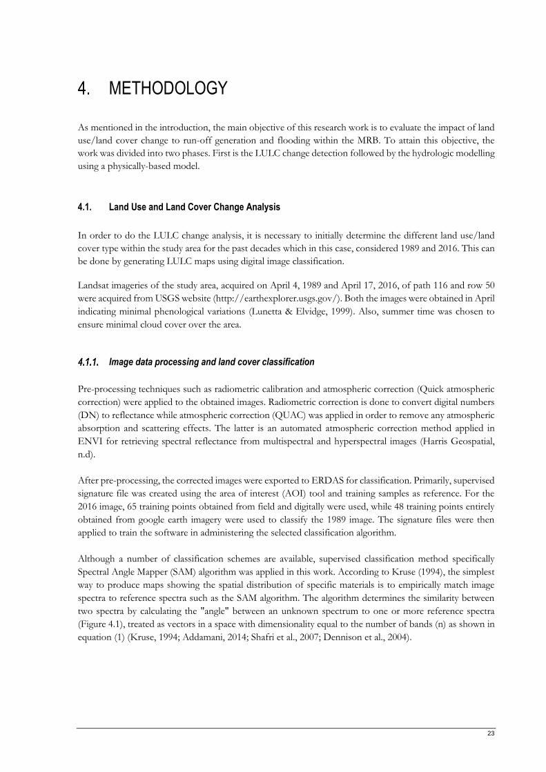
As mentioned in the introduction, the main objective of this research work is to evaluate the impact of land
use/land cover change to run-off generation and flooding within the MRB. To attain this objective, the
work was divided into two phases. First is the LULC change detection followed by the hydrologic modelling
using a physically-based model.
4.1. Land Use and Land Cover Change Analysis
In order to do the LULC change analysis, it is necessary to initially determine the different land use/land
cover type within the study area for the past decades which in this case, considered 1989 and 2016. This can
be done by generating LULC maps using digital image classification.
Landsat imageries of the study area, acquired on April 4, 1989 and April 17, 2016, of path 116 and row 50
were acquired from USGS website (http://earthexplorer.usgs.gov/). Both the images were obtained in April
indicating minimal phenological variations (Lunetta & Elvidge, 1999). Also, summer time was chosen to
ensure minimal cloud cover over the area.
Image data processing and land cover classification
Pre-processing techniques such as radiometric calibration and atmospheric correction (Quick atmospheric
correction) were applied to the obtained images. Radiometric correction is done to convert digital numbers
(DN) to reflectance while atmospheric correction (QUAC) was applied in order to remove any atmospheric
absorption and scattering effects. The latter is an automated atmospheric correction method applied in
ENVI for retrieving spectral reflectance from multispectral and hyperspectral images (Harris Geospatial,
n.d).
After pre-processing, the corrected images were exported to ERDAS for classification. Primarily, supervised
signature file was created using the area of interest (AOI) tool and training samples as reference. For the
2016 image, 65 training points obtained from field and digitally were used, while 48 training points entirely
obtained from google earth imagery were used to classify the 1989 image. The signature files were then
applied to train the software in administering the selected classification algorithm.
Although a number of classification schemes are available, supervised classification method specifically
Spectral Angle Mapper (SAM) algorithm was applied in this work. According to Kruse (1994), the simplest
way to produce maps showing the spatial distribution of specific materials is to empirically match image
spectra to reference spectra such as the SAM algorithm. The algorithm determines the similarity between
two spectra by calculating the "angle" between an unknown spectrum to one or more reference spectra
(Figure 4.1), treated as vectors in a space with dimensionality equal to the number of bands (n) as shown in
equation (1) (Kruse, 1994; Addamani, 2014; Shafri et al., 2007; Dennison et al., 2004).

24
where: n : number of bands
t : pixel spectrum
r : reference spectrum
SA : spectral angle (1)
Smaller angles denotes closer matches to the reference spectrum (Shafri et al., 2007). This algorithm is
adopted in this research work as it is considered as a very powerful classifier because it is not affected by
solar illumination factor and also contains the influence of shading effects to highlight the target reflectance
characteristic (Moughal, 2013).
Additional steps were also undertaken in ARCGIS to improve the classified image. Conditional statements
were generated to incorporate a priori knowledge about the study area using information on elevation
(DEM) and slope (e.g. Con((iff 2016 classified image=agriculture & (DEM>200), forest, 2016 classified image).
Finally, 3x3 major filtering was also performed to both images to remove isolated pixels or noise. After this,
accuracy assessment was carried out using 48 and 40 test pixels collected during fieldwork and digitally, for
the 2016 and 1989 classified image, respectively, as presented in chapter 5.
Land cover/land use change analysis
Once the independently classified image of 1989 and 2016 LULC maps are prepared, the work proceeds to
detecting land use/land cover change which is an integral part of this research work in order to establish a
relation and better understanding on the influence of different land cover types to overland flow generation.
Changes can either be triggered naturally or anthropogenically. In this present work, the observed changes
will be correlated to the socio-economic factor that could have influence such changes.
In this study, the post classification approach was used to analyse the changes of land cover types in MRB.
Post classification comparison technique is the most widely used method for change detection as there is
no need for co-registration of images involved, it has low sensitivity to spectral variation and provides a
“from-to” change information (Raja et al., 2013). Emphasis was given to the significant change of forest
Figure 4.1 SAM algorithm representation (ITC, 2016)
25
cover in the upper reaches of catchment and of built-up areas in the lower portion wherein there was a
substantial decrease and increase, respectively between 1989 and 2016. The change detection analysis was
implemented in ERDAS Imagine with the use of change matrix tool.
4.2. Data Collection and processing
Fieldwork
A three-week field activity was undertaken from September 16 to October 9, 2016 to collect primary and
secondary data such as soil samples, ground truth data for image classification, hydrometeorological data
and other research-related maps and documents. Coordination was initially done with colleagues from the
University of the Philippines-Diliman to get preliminary information as basis for field survey within the
study area. Soil core samplers and Global Positioning System (GPS) unit were the basic instruments used in
the field. In addition, ancillary information were also obtained from various institution and government
agencies to supplement the data needed for this research work.
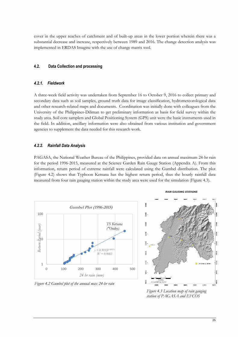
Rainfall Data Analysis
PAGASA, the National Weather Bureau of the Philippines, provided data on annual maximum 24-hr rain
for the period 1996-2015, measured at the Science Garden Rain Gauge Station (Appendix A). From this
information, return period of extreme rainfall were calculated using the Gumbel distribution. The plot
(Figure 4.2) shows that Typhoon Ketsana has the highest return period, thus the hourly rainfall data
measured from four rain gauging station within the study area were used for the simulation (Figure 4.3).
y = 0.5032e0.0083x
R² = 0.9682
1
10
100
0 100 200 300 400 500
Ret
urn
Per
iod
(yea
r)
24 hr rain (mm)
Gumbel Plot (1996-2015)
TS Ketsana("Ondoy)
Figure 4.2 Gumbel plot of the annual max 24-hr rain
Figure 4.3 Location map of rain gauging station of PAGASA and EFCOS

26
Apart from using measured rainfall data of the specific rain event of Typhoon Ketsana, design storms were
generated for simulating the hydrologic processes in the study area to evaluate its response to different
intensities of various storm return period. Utilization of design storms in a particular rainfall-run off model
may contribute largely to flood management and land use or mitigation plans. In this work, 5-, 10- and 20-
year design storms were generated using the intensity-duration-frequency (IDF) relationships, based on a 41
years of rainfall record (1969 – 2010) from the Science Garden Rain Gauging Station in Diliman, Quezon
City (Table 4.1).
Table 4-1 24 hours-RIDF data from Science Garden Rain Gauge Station, Diliman, QC (Source: PAGASA)
Computed Extreme Values (in mm) Precipitation
T (yrs) 10 min 20 min 30 mins 1 hr 2 hrs 3 hrs 6 hrs 12 hrs 24 hrs
2 23 33.4 41.2 55.5 76.7 90.3 117.4 136.3 156
5 31.4 45.5 57.6 81.8 113.2 135.7 185.1 216.1 243.1
10 37 53.6 68.5 99.3 137.5 165.8 229.9 268.9 300.7
15 40.1 58.1 74.6 109.1 151.1 182.7 255.2 298.8 333.3
20 42.3 61.3 78.9 116 160.7 194.6 272.9 319.6 356
25 44 63.7 82.2 121.3 168.1 203.8 286.5 335.7 373.6
50 49.2 71.2 92.4 137.6 190.8 231.9 328.5 385.2 427.6
100 54.4 78.7 102.5 153.8 213.3 259.9 370.2 434.4 481.2
Equivalent AVERAGE INTENSITY (mm/hr) of Computed Extreme Values
T (yrs) 10 min 20 min 30 mins 1 hr 2 hrs 3 hrs 6 hrs 12 hrs 24 hrs
2 138 100.2 82.3 55.5 38.3 30.1 19.6 11.4 6.5
5 188.4 136.6 115.2 81.8 56.6 45.2 30.8 18 10.1
10 221.8 160.7 136.9 99.3 68.7 55.3 38.3 22.4 12.5
15 240.7 174.2 149.2 109.1 75.6 60.9 42.5 24.9 13.9
20 253.8 183.8 157.8 116 80.4 64.9 45.5 26.6 14.8
25 264 191.1 164.4 121.3 84 67.9 47.7 28 15.6
50 295.3 213.6 184.8 137.6 95.4 77.3 54.7 32.1 17.8
100 326.4 236 205 153.8 106.7 86.6 61.7 36.2 20.1
Alternating block method was used to generate the design storm hyetograph derived from the IDF curves
(Figure 4.4). Given the duration and intensity, precipitation depth (mm) was consequently calculated using
the formula, P = I*Td, where I is the intensity
(mm/hr) and Td is the duration (hr). Incremental
rainfall is then computed by taking the
differences between successive precipitation
depth values and used to calculate the intensities
for each time-step. A design intensity hyetograph
in 10-min increments for a 4 hour-storm was
generated by reordering the incremental intensity
blocks in a symmetrical format on the time axis
with the maximum at the middle (Figure
4.5)(Olivera, Stolpa, Assistant, & Manager, 2002).
Figure 4.4 Intensity-Duration-Frequency Curves of the Science Garden Station

27
0
20
40
60
80
100
120
140
160
180
200
0 20 40 60 80 100 120 140 160 180 200 220 240 260
Inte
nsi
ty (
mm
/hr)
time (min)
5Y-RP Design Storm
0
50
100
150
200
250
300
0 20 40 60 80 100 120 140 160 180 200 220 240 260
Inte
nsi
ty (
mm
/hr)
time (min)
10Y-RP Design Storm
0
50
100
150
200
250
300
350
0 20 40 60 80 100 120 140 160 180 200 220 240 260
Inte
nsi
ty (
mm
/hr)
time (min)
20Y-RP Design Storm
(a)
(b)
(c)
Figure 4.5 Design hyetographs of the Marikina River Basin for (a) 5y-return period; (b) 10y-return period and (c) 20y-return period

28
Digital Elevation Model (DEM) Generation
Two sets of digital elevation data were used in this study: 1-m resolution LiDAR DEM, provided by the
National Mapping and Resource Information Authority (NAMRIA) and 30 m SRTM DEM, acquired from
USGS website (https://earthexplorer.usgs.gov/). The LiDAR elevation data only covered the lower part of
the catchment (Figure 4.6a) while SRTM DEM has a full coverage of the study area.
To keep the significant information within the floodplain from LiDAR, a mosaic of the both DEMs was
used for this research work. LiDAR DEM was initially resampled to 30-meter resolution using bilinear
interpolation in ArcMap that uses the distance-weighted average of four nearest pixel values to estimate a
new pixel value. This interpolation method leads to smoother images and represent topography with gradual
change (ITC Core Book, 2012). After resampling, both DEM (LiDAR and SRTM) were stitched together
by means of mosaic tool in ArcGIS to cover the whole watershed area (Figure 4.6b). Margin of the mosaic
image was examined for any abrupt changes that may affect the simulation.
Furthermore, infrastructures such as roads, dikes and embankments also play a significant role during flood
events by influencing overland flow routes. To retain information of these features, vector file of road
networks and dikes/levees particularly within the floodplain were obtained from Open Street Map (OSM)
and Google Earth image. The vector file (polyline) was converted to 1-m resolution raster and then to points
which correspond to each 1-m pixel of LiDAR DEM (Figure 4.7a). Elevation data of each point was
extracted from the LiDAR DEM using a spatial analyst tool in Arcmap (extract values to points). This was
followed by final conversion to raster dataset and resampling to 30-meters wherein cell value assignment
was based initially on the maximum/minimum value of the elevation attributes of the points within the cell
(Figure 4.7b).
a b
Figure 4.6 (a) 1-m resolution LiDAR DEM; (b) Mosaic of resampled LiDAR DEM with 30-m SRTM
29
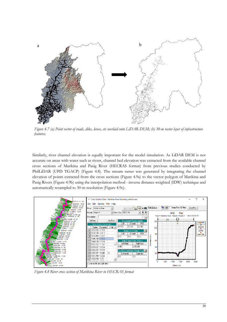
Similarly, river channel elevation is equally important for the model simulation. As LiDAR DEM is not
accurate on areas with water such as rivers, channel bed elevation was extracted from the available channel
cross sections of Marikina and Pasig River (HECRAS format) from previous studies conducted by
PhilLiDAR (UPD TGACP) (Figure 4.8). The stream raster was generated by integrating the channel
elevation of points extracted from the cross sections (Figure 4.9a) to the vector polygon of Marikina and
Pasig Rivers (Figure 4.9b) using the interpolation method - inverse distance weighted (IDW) technique and
automatically resampled to 30-m resolution (Figure 4.9c).
a b
Figure 4.7 (a) Point vector of roads, dike, levees, etc overlaid onto LiDAR DEM; (b) 30-m raster layer of infrastructure features;
Figure 4.8 River cross section of Marikina River in HECRAS format

30
Ultimately, the final DEM was created by incorporating the Mosaic DEM with the infrastructure and main
channel raster layer using cell statistics in Arcmap (Figure 4.10). This tool calculates a per-cell statistics from
multiple rasters. In this case, maximum and minimum cell statistics were used for the integration of infra
layer to DEM and minimum cell statistics for the main channel elevation.
FINAL DEM
LIDAR DEM
SRTM DEM
Infra Layer
Main channel elevation
e
a b c
Figure 4.9 (a) point vector of channel elevation extracted from cross section; (b) digitized river channel of Marikina and Pasig river; (c) 30-m resolution stream layer with interpolated channel bed elevation
Figure 4.10 Final Digital Elevation Model (DEM) generated from the integration of LIDAR, SRTM, road/dikes and channel depth from cross sections

31
Soil data analysis
Published soil texture and soil series maps covering the whole country were readily available at the
Department of Agriculture – Bureau of Soils and Water Management (DA-BSWM) from which information
of the study area was extracted. Moreover, soil physical properties of various soil series area such as saturated
hydraulic conductivity (Ksat), bulk density and soil texture were also gathered from the same agency.
Based on the provided soil data, twenty four (24) undisturbed samples were gathered from accessible areas
in the field which will represent the different soil types. Soil sampling was done using the stratified sampling
approach wherein sampling point locations were based on the soil texture units (Figure 4.11).
Analysis was done in ITC Geoscience laboratory which includes measurement of saturated hydraulic
conductivity, bulk density, soil moisture and soil texture. Initially, the 24 samples were weighed to get the
approximate initial moisture content and were fully saturated for 24 hours in a water tub as required by the
method.
In determining saturated hydraulic conductivity of the samples, a laboratory permeameter was utilized using
the constant water head method. Darcy’s Law is used to calculate the K-factor in this type of method to
determine permeability (Operating Instructions Manual) (2).
V = K * i * A * t K = V * L
A * t * h (2)
Where: V = volume volume of water flowing through the sample (cm3)
K = permeability coefficient or “K-factor” (cm/d)
i = permeability rise gradient, or: h / L (-)
A = cross-section surface of the sample (cm2)
t = time used for flow through of water volume V (d)
(d = time dimension day)
L = length of the soil sample (cm)
h = water level difference inside and outside the ring holder or sample cylinder (cm)
Textural analysis for 7 samples and 5 duplos was carried out to verify the textural identification of the
representative selected samples according to the existing soil map. Primarily, the samples were oven dried
for 24 hours and sieved to remove particles >2mm which was then weighed to determine its percentage
Figure 4.11 (L - R) Undisturbed soil sampling; Identification land cover training data; sheet flooding during the fieldwork

32
within the sample. After the removal of larger particles, ~20 g fine earth materials was taken from the sieved
fraction and was pre-treated to ensure complete dispersion of the primary particles. The pre-treatment stage
entailed removal of organic matter and cementing materials such as calcium carbonate through oxidation.
Sand-size particles were then sieved out using a 50μm sieve while the remaining silt and clay were further
analyse using pipette method to determine fractions of <50 μm (silt), <20 μm (silt) and <2 μm (clay).
Determination of sand fractions was obtain through sieving using mesh sizes from 1000 μm to 50μm.
Finally, calculation was done to all the oven dried fractions using the formula given in the manual provided
by ITC (Appendix B). Organic matter content was also determined using the Walkley Black method or by
careful ashing & weighing (ITC Particle Size Analysis Manual) (Figure 4.12).
4.3. Rainfall-runoff-flashflood modelling
For rainfall-runoff modelling OpenLISEM was selected to simulate different scenarios. It is an open source
model which can simulate soil erosion and run-off during and immediately after a rainfall event (Baartman
et al., 2013). Moreover, as it is a physically-based hydrologic and erosion model, parameters can be
accustomed to the existing condition of the study area. For this research, only the rainfall runoff is given
focus, thus the soil erosion part of the model was disregarded. Processes that were incorporated in the
model include rainfall, interception, infiltration, surface storage, overland flow, channel flow and water
discharge (Figure 4.9). This model works by computing rainfall and interception by vegetation in each raster
grid cell according to the input maps considered. Subsequently, infiltration and surface storage are subtracted
to give the net runoff and water routing to the outlet point is based on the kinematic wave principle (Jetten,
2002). OpenLISEM operates at a catchment scale and is completely incorporated in a raster Geographical
Information System (GIS) – PCRaster (De Roo et al., 1996).
Data preparation
OpenLISEM requires numerous basic input maps and data to better represent the catchment condition
(Figure 4.13). Initially, all input database such as DEM, soil map, LULC maps, outlet map, outpoint map,
road map, NDVI map, boundary map, barrier map, etc were initially prepared in ERDAS Imagine and
ARCGIS interface and resampled to 30-m cell grid size. All of the raster maps were converted to ASCII
Figure 4.12 (left to right) Laboratory permeameter used for Ksat determination; Pipette analysis for fine particle size determination; sieving machine for sand-size particle determination (Source: ITC Laboratory Manual)

33
format and imported to PCraster where the final OpenLISEM input database will be generated using a
revised script for final conversion to the format required by the model (Appendix C).
Rainfall
Essentially, high temporal event-based rainfall data in a time series format is needed. On the other hand, for
the design storm generation, intensity-duration-frequency data is required. In addition, location of rain
gauges where rainfall data was measured is necessary to delineate the rain zone (refer to Figure 4.3). To take
into account the rainfall spatial variability within the watershed, rainfall map for scenarios 1 and 2 was
generated using Thiessen polygons method in interpolating data from the four meteostations (Aries, Boso-
boso, Mt. Oro and Nangka Stations). On the contrary, for scenarios 3 to 5, it was assumed that the whole
catchment will have an equal rainfall distribution using the design storm generated from one rain gauge
station (Science Garden Station) (Figure 4.14).
Figure 4.13 (Left) Flow chart of LISEM Model (adapted from De Roo & Jetten, 1999); (Right) General data requirement for OpenLISEM (Jetten & Shrestha, 2016)
Figure 4.14 Id map to indicate rainfall distribution for scenarios 1 & 2 (left) and 3 - 5 (right)

34
For every time increment during the simulation of a storm, the model generates a map with the spatial
distribution of the rainfall intensity using a single statement that uses the rain gauge identification map and
the time series file. Thus, the model allows for spatial and temporal variability of rainfall (De Roo, Wesseling,
& Ritsema, 1996).
Interception
The first process that happens with rainfall is interception by the canopy of natural vegetation and crops.
For this, vegetation/crop maps were prepared initially by determining the cover fraction (C) (Figure 4.15)
from the normalized difference vegetation index (NDVI) (Knijff et al., 1999). Leaf area index (LAI) (Figure
4.16) is then derived from cover fraction which is used to calculate the maximum storage capacity (SMAX)
(Figure 4.17). The variables mentioned were calculated using the following equations as shown in Table 4-
2.
Table 4-2 Equations used in deriving interception variables Variables Equation
Normalized Difference
Vegetation Index
(NIR – Red)
(NIR + Red)
Cover Factor C = 1 - exp(-α*NDVI)/(β-NDVI)
where α,β are parameters that determine the shape of the NDVI curve which in this
case an α-value of 2 and β-value of 1.5 were used
Leaf Area Index LAI = ln(1-C)/-0.4
Maximum Storage
Capacity
Smax (Forest) = 0.2856 * LAI
Smax (Shrub) = 0.1713 * LAI
Smax (Grass) = 0.912 * ln(LAI) + 0.703
Smax (Crops) = 0.935+0.498 * LAI-0.00575 * (LAI)2
NDVI =
Figure 4.15 Vegetation cover fraction in 1989 (left) and 2016 (right) calculated based on NDVI

35
Figure 4.16 Leaf area index (LAI) in 1989 (left) and 2016 (right)
Figure 4.17 Interception storage capacity (Smax) in 1989 (left) and 2016 (right)

36
Infiltration and Surface Storage
Part of the rainfall not intercepted by canopy either infiltrates to the soil or stored at the surface. The rate
of infiltration depends largely on soil physical properties and land use/land cover. This is simulated by
OpenLISEM using the Green and Ampt infiltration equation which describes how water enters the soil
from a simple application of Darcy’s law (Van Mullem, 1991) (3).
Where f = surface infiltration rate
Ksat = saturated hydraulic conductivity
dh = suction exerted by the soil
dz = distance from the surface over which
the suction is applied
1 = gravity (constant) (3)
These parameters are all inherent to the underlying soil within the study area, thus information on physical
soil characteristics (Ksat, porosity, initial moisture, wetting front suction and texture) are vital. In this work,
values for the mentioned parameters were obtained from laboratory results supplemented by published data
of the Department of Agriculture - Bureau of Soils and Water Management and other related literature
(Rawls et al., 1983) (Table 4.3). The following parameters were basis for the generation of the infiltration-
related maps such as Ksat map, saturated volumetric soil moisture content map, initial volumetric soil
moisture content map and soil water tension at the wetting front map.
Table 4-3 Soil physical parameter values
Texture Bulk Density
(g/cm3) Porosity
Ksat
(mm/hr)
Initial Soil
Moisture
Wetting Front
Suction (cm)
Novaliches Loam 1.25 0.53 3 0.20 8.89
Novaliches Clay Loam 1.25 0.53 3 0.20 20.8
Antipolo Soil (undiff) 1.52 0.43 43 0.29 27.3
Antipolo Clay 1.3 0.51 0.43 0.34 31.6
Binangona Clay 1.35 0.49 0.1 0.22 31.6
Marikna Clay Loam 1.25 0.53 3 0.16 20.8
Marikina Silt Loam 1.3 0.51 0.64 0.33 16.6
Marikina Loam 1.45 0.45 4.6 0.19 8.9
Novaliches Clay Loam Adobe 1.48 0.44 9.9 0.19 20.8
Quiangua Silt Loam 1.3 0.51 12 0.14 16.6
Antipolo Clay Loam 1.4 0.47 12 0.26 20.8
Guadalupe Clay Adobe 1.48 0.44 9.9 0.20 4.9
Guadalupe Clay 1.28 0.51 0.61 0.25 31.6
Bay Clay Laom 1.25 0.53 3 0.27 20.8
Also, hard surfaces such as roads affect infiltration of water. In this model, road layer was acquired from
openstreet map and classified into primary, secondary and tertiary roads. The width of each section were
approximate measurement based from google earth image ranging from 3 meters to 30 meters (Figure 4.18).

37
Overland Flow
When infiltration and saturation is exceeded, overland flow (surface runoff) is generated. Runoff velocity
and flow direction vary spatially and is mainly determined by the terrain conditions which also defines the
channel network. Likewise, surface roughness expressed by Manning’s n and random roughness (rr) also
influence the flow of runoff and this value differs depending on land cover type (Table 4.4). Manning’s n
values of the existing land cover types in the area were obtained from literature (Chow, 1959).
Table 4-4 Land cover type parameters that influences runoff velocity Land cover type Plant height Random Roughness (RR) Manning’s n Forest 20 1.5 0.1
Shrub 3 1.5 0.1
Grass 1 1.5 0.035
Agriculture 0.5 1.8 0.035
Built-up 0 0.7 0
Water body 0 0 0
Channel Flow
Data required in this part include DEM which is used to derive input maps such as the local drain direction
map (ldd). The ldd map gives each cell the direction of runoff towards the channel network. The channel
network was defined by using OSM data, however, channels at the lower catchment were modified in
ARCGIS by adjusting the polylines based on the LIDAR DEM (Figure 4.19). In addition, channel width
was also approximated from the LIDAR DTM. On the other hand, to define channel properties, constant
values were considered in the calculation such as channel cohesion, Manning’s n value of channel, channel
side angle, channel saturated hydraulic conductivity and minimum slope (Table 4-5).
Figure 4.18 Road layer map showing road width in meters

38
Table 4-5 Constant values used to define channel properties
Figure 4.19 Channel work of the study area
Water Discharge To provide location points of measurement for the model simulation, three outpoints were defined in this work (Figure 4.20). Outpoint 1 is located at the base of the upper catchment as to differentiate the influence of land cover changes upstream in terms of discharge and water level along the channel. Outpoint 2 is located at the flood plain section while outpoint 3 is the main outlet and is located at the eastern edge of the watershed boundary.
Property Value
Channel cohesion (kPa) 8
Channel Manning’s n 0.04
Channel side angle 0
Channel Ksat 1
Minimum slope 0.002
Figure 4.20 Location of outpoints

39
Flood Model Development
Once all input maps and rainfall table are prepared, these are then inputted to OpenLISEM interface. For the simulation, the run file used is luse50m.run which contains all the options and map names of a single run whereas the rainfall file selected depends on the scenario being simulated.
Primarily, flood simulation was carried out using the rainfall data of Typhoon Ketsana in 2009 and 2016
database. For this, hourly data from four (4) rain gauging stations (Aries, Boso-boso, Mt. Oro and Nangka
Stations) within the catchment was provided by Metro Manila Development Authority – Effective Flood
Control Operation System (MMDA-EFCOS) (Refer to Figure 4.3). The 42-hours rainfall which covered the
duration from September 25 (1400H) to September 27 (0800H) was specifically used in the simulation. The
results of the initial run was then calibrated by comparing simulated water level with measured water level
at Sto. Niño gauging station. Once satisfied with the calibration result, the modified parameters will then be
utilized in running the model for the simulation of flood event using the 1989 database.
Additionally, 5-, 10- and 20-year return period rain events generated from Intensity-Duration-Frequency
(IDF) curves were also used in simulating flood scenarios. IDF Curves are derived from the statistical
frequency analysis of rainfall records over a period of time (Subyani & Al-Amri, 2015), which in this case is
1969-2010, measured from one gauging station (Science Garden Station) in Diliman, Quezon City operated
by the Philippine Atmospheric, Geophysical and Astronomical Services Administration (PAGASA). IDF
relationships are usually in a graphical form with duration plotted on the horizontal axis, intensity on the
vertical axis and a series of curves for each design return period (Chow et al., 1988). The design storms with
a 10-minute interval were generated using this information. The hyetographs of the selected design storm
were produced using the alternating block method which consist of incremental precipitation depth blocks
placed on the time axis to generate the greatest precipitation depth for all durations shorter than the storm
duration (Olivera et al., 2002).
In Figure 4.21, a simplified flowchart for running different flood scenarios is given. Five simulations were
run in openLISEM in order to answer the related research questions. These scenarios are based on different
LULC maps (1989 and 2016) and three design storms.
Scenario 1: Flood simulation using 1989 LULC map and rainfall data of Typhoon Ketsana (2009)
Scenario 2: Flood simulation using 2016 LULC map and rainfall data of Typhoon Ketsana (2009)
Scenario 3: Flood simulation using 2016 LULC map and rainfall data of 5YR- return period design storm
Scenario 4: Flood simulation using 2016 LULC map and rainfall data of 10YR- return period design storm Scenario 5: Flood simulation using 2016 LULC map and rainfall data of 20YR- return period design storm

40
Figure 4.21 Flow chart showing the simplified methodology of the research work

41
RESULTS AND DISCUSSION
5.1. Land use and land cover Classification
For the LULC classification of 1989 and 2016 Landsat images (Figure 5.1) using spectral angle mapper
(SAM) algorithm, six (6) general categories of land cover were distinguished based on a-priori knowledge of
the area and previous studies which include forest, shrub, grass, agriculture, built-up and water body (Abino
et al., 2015) (Figure 5.2). Classified maps show that grassland was the dominant land cover type in both
years. In 1989, forest was the second extensive land cover followed by shrub, built-up, agriculture and water
body as the least. However, in 2016, forest was replaced by built-up and shrub while agriculture and water
body are the least land cover type (Table 5.1).
Figure 5.1 (Left) Landsat TM 7 satellite image of the study area in 1989; (Right) Landsat OLI-8 image of MRB in 2016
Table 5-1 Total Area coverage of various land cover types
LULC Class 1989 2016
Area (hectares)
Forest 18, 683 13,350
Shrub 14,470 13,197
Grass 20,841 21,640
Agriculture 2,850 3,832
Built-up 11,928 16,952
Water Body 821 622

42
Tables 5.2 presents the producer’s and user’s accuracy statistics and error matrix, respectively of 1989 image
while tables 5.3 shows the results for 2016 image. Result of the accuracy assessment using 40 test pixels for
1989 shows an overall accuracy of 70% was reached with an overall Kappa (K^) statistics of 0.6404. For
2016, 48 test pixels were used and yielded an overall accuracy of 77.08% and K^ statistics of 0.7202.
Table 5-2 Error Matrix and accuracy report for 1989 classified image
Land Cover
Fo
rest
Sh
rub
Gra
ss
Ag
ricu
ltu
re
Bu
ilt-
up
Wat
er b
od
y
Cla
ssif
ied
T
ota
ls
Ref
eren
ce
To
tals
Nu
mb
er
Co
rrec
t
Pro
du
cers
A
ccu
racy
Use
rs
Acc
ura
cy
Forest 6 4 0 0 1 0 11 7 6 85.71% 54.55%
Shrub 1 1 2 0 0 0 4 8 1 12.50% 25.00%
Grass 0 3 3 0 0 0 6 5 3 60.00% 50.00%
Agriculture 0 0 0 6 0 0 6 7 6 85.71% 100.00%
Built-up 0 0 0 0 6 0 6 7 6 85.71% 100.00%
Water Body
0 0 0 1 0 6 7 6 6 100.00% 85.71%
Totals 7 8 5 7 7 6 40 40 28 Overall Classification
Accuracy 70.00%
Figure 5.2 Land cover map of MRB in 1989 and 2016 generated from Landsat imageries

43
Table 5-3 Error Matrix and accuracy report for 2016 classified image
Based on the matrices, it shows that in general, the classification accuracy of shrub and grass is relatively
low. This could be explained due to overlapping occurrence of these land covers. On the field, grass and
shrub occur as intergrowth in very close range, thus, labelling of entire 30-m pixel to one category will result
to some error. Moreover, the insufficiency of test samples per category may also be a limitation as not all
spectral signatures of each category could have been represented.
5.2. Land cover change detection
The independently generated LULC maps were then subjected to change detection analysis in ERDAS
Imagine using post classification method specifically matrix union and summary report of matrix function
as described in section 4.1.2. The former produced an output image file which shows how classes between
the two images overlap. The summary report produced a cross-tabulation statistics between the two
thematic image file which shows a “from-to” change of classes in either number of points, area or
percentage.
The summary matrix of the post classification method displays the change of land cover based land area in
hectare (Table 5.4) wherein each column for every land cover type totals to the area covered in 1989, while
the rows show the area of change from one class to another.
Based on the analysis, the highest general change (excluding water body) was on the agricultural land wherein
of its original 2,849 hectares in 1989, about 2,156 hectares was converted into a different land cover. The
largest conversion of agricultural land was into built-up area which accounts to a sizeable portion of 1195.47
hectares. This may be attributed to the high demand and value of land for residential projects like
subdivisions and condominiums as well as commercial buildings. Forest and shrubs were mainly changed
to grassland that may be due to some slash and burn practices (“kaingin”) or clearing.
Comparison of gain and loss reveals that forest cover has the largest loss in terms of area from 1989 to 2016
of about 5,333 hectares, followed by shrub with 1,272 hectares loss. Built-up on the other hand, gained an
additional area of about 5,023 hectares followed by agriculture and grass which gained 982 hectares and 798
Land Cover
Fo
rest
Sh
rub
Gra
ss
Ag
ricu
ltu
re
Bu
ilt-
up
Wat
er b
od
y
Cla
ssif
ied
T
ota
ls
Ref
eren
ce
To
tals
Nu
mb
er
Co
rrec
t
Pro
du
cers
A
ccu
racy
Use
rs
Acc
ura
cy
Forest 10 0 0 0 0 0 10 13 10 76.92% 100.00%
Shrub 1 6 1 1 0 0 9 8 6 75.00% 66.67%
Grass 1 1 6 1 0 0 9 9 6 66.67% 66.67%
Agriculture 1 1 1 4 0 0 7 6 4 66.67% 57.14%
Built-up 0 0 1 0 8 1 10 8 8 100.00
% 80.00%
Water Body 0 0 0 0 0 3 3 4 3 75.00% 100.00%
Totals 13 8 9 6 8 4 48 48 37 Overall Classification
Accuracy 77.08%

44
hectares, respectively. However, it should be noted that the result also produced some questionable results
which can be attributed to classification accuracy.
Table 5-4 Summary matrix showing area of land cover change from 1989 to 2016 using post classification method
1989
Area (Hectares)
Land Cover Type Forest Shrub Grass Agricult
ure Built-up
Water Body
GAIN Total Area
2016
Forest 9820.89 513.63 2843.01 68.67 58.32 45.45 3529.08 13349.97
Shrub 3178.98 7133.04 2139.84 336.69 373.14 35.73 6064.38 13197.42
Grass 4836.69 3268.89 12158.82 525.96 784.44 64.98 9480.96 21639.78
Agriculture 193.32 877.86 1335.96 692.82 621.18 110.61 3138.93 3831.75
Built-up 627.93 2593.26 2257.2 1195.47 9998.28 280.17 6954.03 16952.31
Water Body 25.29 83.52 106.65 30.15 92.97 283.77 338.58 622.35
Total Area 18683.1 14470.2 20841.48 2849.76 11928.33 820.71
LOSS 8862.21 7337.16 8682.66 2156.94 1930.05 536.94
Visual inspection and comparison between 1989 LULC map and 2016 LULC map shows that there is a
significant increase of built-up areas north-eastward (Figure 5.3a). Analysis of the socioeconomic status
within the watershed reveals that increase of population growth rate can also be observed in the similar
areas. Expansion of land development particularly subdivisions is attributed to the increasing population
and high market value which is also likely related to industrialization. According to the Formulation of an
Integrated River Basin Management and Development Master Plan for Marikina River Basin, industrial land
and commercial areas have been rapidly developing in the past 10 years.
Moreover, there was also a considerable decrease of forest cover from 18,683 hectares in 1989 to 13,350
hectares in 2016 (Figure 5.4a). As per DENR report (IRBMP, 2015), small-scale charcoal making and
“kaingin” contributed to the degradation and deforestation of the upper reaches of the catchment. Change
analysis shows that large portion of the forest cover in 1989 became shrub and grassland while areas at the
lower catchment has been converted to built-up area which increase (Figure 5.4b).
Figure 5.3 Spatial distribution of built up areas within the last 3 decades

45
5.3. Rainfall-runoff modelling and calibration
Rainfall-runoff and flashflood simulation was carried out using the actual extreme rainfall of Typhoon
Ketsana in 2009. The model generates a hydrograph which shows rainfall and discharge against time as well
as information on channel water height. The result of the model was compared to a set of measured values
of water level from Sto. Niño gauging station for calibration. Calibration is done in order to achieve an
acceptable level of predictive quality and optimize the parameter setting (ITC Core Book, 2012). In this
research, optimization of parameters was performed by fine tuning the Ksat values and Manning’s n of both
slopes and channel. These parameters both influence the infiltration rate, surface runoff generation and
response time of discharge.
The measured water level in Sto. Niño gauging station included the base flow height within the channel, as
such, the values were subtracted with the assumed base flow level prior to the flooding event which is 15.8
meters. Moreover, the measured water level values considered in the calibration only covered the time period
from 0500H (900 min) to 1800H (1680 min) as no measurement was available after the last record.
However, due to time constraints, calibration done by trial and error method was limited by generating a
hydrograph with a closest fit to the observed water level which in this case was obtained by using a
multiplication factor of 2.0 for both Manning’s n and Ksat (Figure 5.5).
Figure 5.4 (a) significant decrease of forest cover from 1989 to 2016 shown spatially; (b) conversion from forest cover to other land covers
a b

46
Figure 5.5 OpenLISEM calibration result showing the nearest simulated curve (green) to the measured water level value at Sto. Niño Gauging station
5.4. Impact of Land use/ Land cover
In this research, the impact of LULC change on runoff generation was assessed by simulating flood
scenarios using similar rainfall data to different LULC map from two periods. Earlier analysis of satellite
images verified the significant changes in land cover from 1989 to 2016 particularly at the upper reaches of
the watershed from forest to shrub/grass while change from agriculture to built-up was noted within the
floodplain of the catchment.
As illustrated in section 4.3.1, decrease in vegetation cover is in accord with the increase of built up area.
The reduction of cover is associated to the decrease in leaf area index (LAI) (see Figure 4.16) which
determines the interception storage capacity especially in the upper catchment (Figure 4.17). In the study
of Siriwardena et al. (2006), they concluded that the impact of clearing forest vegetation in the Comet
catchment in Central Queensland from 83% to 38% increase the runoff by about 40%. This was also
established in the work of Lin & Wei (2008) where they correlated the decrease of forest to the significant
increase in peak and mean flows
In this study, it can be noted that vegetation cover in 1989 is widespread as compared to 2016, thus, it is
expected that run-off will also be low during this period due to high vegetation interception. To assess
whether this concept holds true to my study area, it is necessary to quantify the effect of land cover change
particularly upstream which is considered as the run-off originating zone (Wang et al., 2006b). In doing so,
outpoint 1 (refer to Figure 4.20) was used to record the simulated peak time and peak discharge of scenarios
1 and 2 as described in section 4.3.2.
When the rainfall-runoff model was run using the 27 hour rainfall duration with an average total rainfall of
about 300mm on the land cover map of 1989, the peak discharge was 18m3/s with peak time at 1328
0
10
20
30
40
50
60
70
80
0
1
2
3
4
5
6
7
8
900 1400 1900 2400 2900
Rai
nfa
ll (m
m/h
)
Wat
er L
evel
(m
)
Duration (min)
Hydrograph of Water Level
Simulated WL (1.0)
Simulated WL (2.0)
Measured WL
P (mm/hr)

47
minutes. Using the same rain event on 2016 land cover map, the peak discharge generated was 16m3/s with
peak time at 1211 minutes (Figure 5.6).
Result shows that the decrease of forest cover in 2016 resulted to a slight decrease of runoff and discharge.
This confirms the result of the work of Sriwongsitanon & Taesombat (2011) in which they stated that during
high rainfall intensity events, watershed condition behaves differently especially in catchments with high
antecedent soil moisture. Based on their research, forest area can have high antecedent soil moisture from
previous rain events due to deeper root zone and higher soil moisture holding capacity and will entail less
amount of water to reach saturation stage thus resulting to higher runoff. They concluded that an increase
in forest area also increased the runoff coefficient and increase in non-forest area resulted to lower runoff
coefficient. This is characterized by the total discharge (Qtotal) produced by the model for both dataset, where
Qtotal = 9.4 million m3 and 7.6 million m3 for 1989 and 2016, respectively.
For the downstream part of the catchment, the significant LULC change was the increase of built up areas
from 17% of the total area in 1989 to 24% 2016. Urbanization in the floodplain adversely influence the
hydrological processes in the lower catchment by decreasing the infiltration capacity of the underlying soil
attributed to the increase of impervious surfaces. This will result to higher runoff thus enhancing flood
volume and extent. Model output shows that the peak discharge and peak time measured in outpoint 2 (refer
to figure 4.20) on 1989 LULC map was 103 m3/s at 1561 minutes while on 2016 LULC was 116 m3/s at
1566 minutes (Figure 5.7). Flood volume and flooded area in 1989 is 84.3 million m3 and 103.4 million
m2, respectively, while for 2016 is 86 million m3 and 103.7 million m2.
90
0
10
00
11
00
12
00
13
00
14
00
15
00
16
00
17
00
18
00
19
00
20
00
21
00
22
00
23
00
24
00
25
00
26
00
27
00
28
00
29
00
0
10
20
30
40
50
60
70
80
0
2
4
6
8
10
12
14
16
18
20
900 1400 1900 2400 2900
P (
mm
/hr)
Dis
char
ge (
m3
/s)
Duration (minutes)
Rainfall Intensity
Outpoint 1 (2016)
Outpoint 1 (1989)
Figure 5.6 Hydrograph of the simulated discharge against rainfall between two years as measured in outpoint 1

48
Moreover, another consequence of reduced infiltration rate is longer flood duration for 2016 as shown in
Figure 5.8. Duration difference of flood between the two scenarios is noticeable wherein a considerable area
in 2016 experienced flood in a longer period as compared to 1989. This is attributable to expansion of built-
up areas wherein the increase of hard surfaces greatly reduced the infiltration rate within the floodplain.
Moreover, intensification of construction may have also lead to the increase of obstruction to surface runoff
thus limiting the flow of water to natural or artificial channels increasing flooding period in the lowland.
90
0
10
00
11
00
12
00
13
00
14
00
15
00
16
00
17
00
18
00
19
00
20
00
21
00
22
00
23
00
24
00
25
00
26
00
27
00
28
00
29
00
0
10
20
30
40
50
60
70
80
0
20
40
60
80
100
120
140
900 1400 1900 2400 2900
P (
mm
/hr)
Dis
char
ge (
m3
/s)
Duration (minutes)
Rainfall Intensity
Outpoint 2 (2016)
Outpoint 2 (1989)
Figure 5.7 Hydrograph of the simulated discharge against rainfall between two years as measured in outpoint 2
Figure 5.8 Flood duration map of 1989 (left) and 2016 (right)

49
The summary of simulation result is presented in Table 5-7. This shows that overall, LULC change has minimal impact on flooding occurrences during extreme condition.
Table 5-4 Results of OpenLISEM flood model
Variable Unit 1989 2016
LISEM results at time min 2,998 2,998
Catchment area Ha 73,334.07 73,334.07
Total Precipitation mm 306.3 306.3
Total discharge mm 23.11 21.10
Total interception mm 0.63 0.63
Total House interception mm 0.10 0.15
Total infiltration mm 146.17 142.41
Surface storage mm 0.02 0.02
Water in runoff + channel mm 22.42 20.93
Total discharge m3 9.4 x 10⁶ 7.6 x 10⁶
Peak time precipitation min 1,201 1,201
Peak discharge/Precipitation % 7.54 6.89
Flood volume (max level) m3 84 x 106 86 x 106
Flood area (max level) m2 103.4 x 10⁶ 103.7 x 10⁶
5.5. Response of large watershed to varying flood return period
To evaluate how a large watershed such as MRB responds to extreme rainfall at different return periods, 4-
hour design rain storms at 10-minutes time steps for 5-yr, 10-yr and 20-yr return period were generated
using IDF curves and alternating block method as illustrated in section 4.2.2. The total precipitation used
for each return period are 138mm (5-yr RP), 169mm (10-yr RP) and 198mm (20-yr RP). Flood simulations
for different return periods were undertaken using LULC map of 2016 in OpenLISEM. Two outlet points
were considered in assessing hydrologic responses of the upper and lower watershed (Figure 5.9).
Figure 5.9 Outpoint locations

50
Result shows that in the upper catchment, the increase of return period only induced a minimal increase on
peak discharge as measured from outpoint 1 (Table 5-6). The peak discharge is highest in the 20y-return
period at 18 m3/s while the lowest is recorded for the 5y-RP at 16 m3/s (Figure 5.10). However, this also
suggests that as rainfall intensity increases, effect of vegetative covers in terms of interception becomes
negligible resulting to more water available for surface runoff.
Table 5-5 Discharge data at outpoint 1
On the other hand, distinct variation on flood characteristics are more observable in the downstream area
as measured at outpoint 2 (Table 5-6). A significant difference on peak discharge and peak timing was noted
wherein increase in return period denotes high peak discharge and shorter response time (Figure 5.11). The
peak discharge and peak timing for 5-, 10- and 20y-RP are 40 m3/s at 498min, 57 m3/s at 448 and 77 m3/s at
426 min, respectively.
Table 5-6 Discharge data at outpoint 2
5y-RP 10y-RP 20y-RP
Peak discharge (m3/s) 15.6 17.3 18.2
Peak time discharge (min) 141 143 148
5y-RP 10y-RP 20y-RP
Peak discharge (m3/s) 40.36 56.88 77.08
Peak time discharge (min) 498 448 426
0
2
4
6
8
10
12
14
16
18
20
0 100 200 300 400 500
Q (
m3
/s)
Duration (minutes)
Q1_5RP
Q1_10RP
Q1_20RP
Figure 5.10 Hydrograph measured at outpoint 1
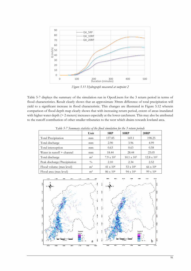
51
Table 5-7 displays the summary of the simulation run in OpenLisem for the 3 return period in terms of
flood characteristics. Result clearly shows that an approximate 30mm difference of total precipitation will
yield to a significant increase in flood characteristic. This changes are illustrated in Figure 5.12 wherein
comparison of flood depth map clearly shows that with increasing return period, extent of areas inundated
with higher water depth (> 2 meters) increases especially at the lower catchment. This may also be attributed
to the runoff contribution of other smaller tributaries to the west which drains towards lowland area.
Table 5-7 Summary statistics of the flood simulation for the 3 return periods
Unit 5RP 10RP 20RP
Total Precipitation mm 137.85 169.1 198.25
Total discharge mm 2.90 3.96 4.99
Total interception mm 0.63 0.63 0.58
Water in runoff + channel mm 18.44 28.44 25.05
Total discharge m3 7.9 x 10⁵ 10.1 x 10⁵ 12.8 x 10⁵
Peak discharge/Precipitation % 2.10 2.34 2.52
Flood volume (max level) m3 41 x 106 53 x 106 66 x 106
Flood area (max level) m2 86 x 106 94 x 106 99 x 106
0
10
20
30
40
50
60
70
80
90
0 100 200 300 400 500
Q (
m3
/s)
Duration (minutes)
Q4_5RP
Q4_10RP
Q4_20RP
Figure 5.11 Hydrograph measured at outpoint 2
a b

52
5.6. Validation of simulated result (2016 Scenario)
The simulated model for scenario 1 using rainfall data during typhoon Ketsana was validated by comparing
the flood depth map with the published flood map of the Mines and Geosciences Bureau (MGB). MGB
flood map is based worst case event in the area and mainly used flood depth and flood duration as
parameters for classification (Appendix D). Comparison of simulated flood depth and flood extent with
MGB flood susceptibility map is illustrated in Figure 5.13.
c
41
53
66
0
20
40
60
80
5RP 10RP 20RP
mill
ion
(m
3 )
Flood Volume
75
80
85
90
95
100
5RP 10RP 20RPm
illio
n (
m2 )
Flooded area
Figure 5.12 Flood depth and flood extent map of (a) 5yr-RP, (b) 10yr-RP and (c) 20yr-RP. Graphs on right illustrates the statistical differences of flood depth and flood extent for the 3 return periods
Figure 5.13 Comparison of simulated flood depth/extent map (left) with MGB flood susceptibility map (right)

53
Validation shows that the simulated result closely resembles the flood susceptibility map in terms of extent.
In terms of flood depth, it can be noted that some portions of the model output have discrepancy as
compared to the delineated zones of MGB. This however, still needs additional validation with flood depth
measurement during the actual flooding event
5.7. Scope and Limitation of the Research
This research covers the MRB with a total area of 698 sq. km. Taking into account the size of the watershed,
the study was limited to few free remotely sensed products to cover the whole area with a reasonable spatial
resolution and high temporal resolution. In this case Landsat TM 5 and OLI-8 with 30-m spatial resolution
were used for the land cover classification.
Moreover, the samples collected from field were not sufficient to represent the different soil types and
landcover types of the area. Therefore, laboratory results of the falling head permeability test for hydraulic
conductivity analysis and soil textural analysis using pipette method were only used for comparison and
confirmation, respectively. Instead, published secondary data were utilized in the parameterization of the
model.
Likewise, effect of structures within the floodplain particularly the Manggahan floodway and Napindan
Channel were disregarded in the flood simulation using the extreme rainfall record during the onset of
typhoon Ketsana (TS “Ondoy”) in 2009. In reality, these two structures influence the discharge and flow
velocity along the main river by diverting flood water to the nearby Laguna de Bay. This could have affected
the total discharge as well as the flood extent and depth in the simulation.
Furthermore, due to time constraints and the period required in undertaking each simulation which is about
72 hours, calibration and validation of the model was limited. In this work, a multiplication factor of 2 for
both Ksat and Manning’s n was considered as the best option for the time being in running the model. This
limitation may introduce some inaccuracies in the reported output of the simulation which will give a
discrepancy from the measured values. More time would have been useful for more intensive model
calibration.
54
CONCLUSION AND RECOMMENDATION
In this research work, a physically-based model – OpenLISEM – was used to simulate the runoff and
flashflood scenarios. As part of the research objective, LULC change was identified between the selected
period (1989 and 2016) to established significant changes within the area. Analysis shows that the most
dominant changes observed are the decrease of forest cover into shrub and grass at the upper reaches of
MRB and the increase of built-up areas at the lowland that compensated the decrease of agricultural area.
In general, these changes are mainly attributed to several driving factors such as human drivers (population
growth), economic conditions and local upland practices (slash and burn).
The OpenLISEM model was able to simulate flood scenarios using the classified LULC map of 1989 and
2016. The result of the study as discussed in previous chapters showed that land use land cover change may
have an influence to flashflood, however, several factors should also be considered. Analysis of the upstream
area concludes that change of vegetative cover will have an insignificant effect to runoff generation during
convective or extreme conditions. In the downstream part, urbanization have an effect on flood extent,
flood volume and flood duration.
Moreover, simulation of scenarios using design storm of 5y-, 10-y and 20-y return period revealed that
increase of rainfall intensity diminishes the influence of vegetative land covers to flood characteristics. In
the contrary, development of infrastructures within the floodplain may impact the routing of runoff which
may ensue changes to other flood properties such as depth, extent and duration.
In conclusion, the work undertaken was able to meet the research objectives in detecting significant land
cover/land use change in MRB and in evaluating the influence of various LULC change to overland flow
with extreme rains of different return periods. However, results of the study and performance of the model
can be further improved if the following are taking into account:
Produce a more accurate LULC maps by imploring other classification algorithms. Additional
images from other periods can also be considered in order to establish a more concrete relationship
between LULC change and runoff-flash flood.
Determine physical soil properties such as saturated hydraulic conductivity of each land
use/landcover per soil type to generate a more accurate representation of the study area
Proper calibration and validation of model output is necessary to be able to generate a more realistic
simulation. Acquisition of a complete data for calibration and validation is also needed
Taking into account the required simulation time needed for this research, improvement to the
model’s algorithm or system can be look into in order to optimize the applicability of the model for
large-scale watershed.

55
LIST OF REFERENCES
Abino, A. C., Kim, S. Y., Jang, M. N., Lee, Y. J., & Chung, J. S. (2015). Assessing land use and land cover of the Marikina sub-watershed, Philippines. Forest Science and Technology, 11(2), 65–75. http://doi.org/10.1080/21580103.2014.957353
Abon, C. C., David, C. P. C., & Pellejera, N. E. B. (2011). Reconstructing the Tropical Storm Ketsana flood event in Marikina River, Philippines. Hydrology and Earth System Sciences, 15, 1283–1289. http://doi.org/10.5194/hess-15-1283-2011
Abon, C. C., Kneis, D., Crisologo, I., Bronstert, A., David, C. P. C., & Heistermann, M. (2016). Evaluating the potential of radar-based rainfall estimates for streamflow and flood simulations in the Philippines. Geomatics, Natural Hazards and Risk, 7(4), 1390–1405. http://doi.org/10.1080/19475705.2015.1058862
Aich, V., Liersch, S., Vetter, T., Fournet, S., Andersson, J. C. M., Calmanti, S., … Paton, E. N. (2016). Flood projections within the Niger River Basin under future land use and climate change. Science of The Total Environment, 562, 666–677. http://doi.org/10.1016/j.scitotenv.2016.04.021
Almeida, C. A. de, Coutinho, A. C., Esquerdo, J. C. D. M., Adami, M., Venturieri, A., Diniz, C. G., … Gomes, A. R. (2016). High spatial resolution land use and land cover mapping of the Brazilian Legal Amazon in 2008 using Landsat-5/TM and MODIS data. Acta Amazonica, 46(3), 291–302. http://doi.org/10.1590/1809-4392201505504
Archer, N. A. L., Bonell, M., Coles, N., MacDonald, A. M., Auton, C. A., & Stevenson, R. (2013). Soil characteristics and landcover relationships on soil hydraulic conductivity at a hillslope scale: A view towards local flood management. Journal of Hydrology, 497, 208–222. http://doi.org/10.1016/j.jhydrol.2013.05.043
Badilla, R. A. (2008). Flood Modelling in Pasig-Marikina River Basin. (MSc Thesis), International Institute for Geo-Information Science and Earth Observation.
Baker, T. J., & Miller, S. N. (2013). Using the Soil and Water Assessment Tool (SWAT) to assess land use impact on water resources in an East African watershed. Journal of Hydrology, 486, 100–111. http://doi.org/10.1016/j.jhydrol.2013.01.041
BBC News. (2014). Retrieved from http://news.bbc.co.uk/2/hi/europe/4913182.stm Beven, K. J., Wood, E. F., & Sivapalan, M. (1988). On hydrological heterogeneity --Catchment
Morphology and Catchment Response. Journal of Hydrology Elsevier Science Publishers B.V, 100, 353–375.
Bi, Y., Zou, H., & Zhu, C. (2014). Dynamic monitoring of soil bulk density and infiltration rate during coal mining in sandy land with different vegetation. International Journal of Coal Science & Technology, 1(2), 198–206. http://doi.org/10.1007/s40789-014-0025-2
Carating, R. B., Galanta, R. G., & Bacatio, C. D. (2012). The Soils of the Philippines. (A. Hartemink, Ed.)National Science …. Dordrecht: Springer London. http://doi.org/10.1007/978-94-017-8682-9
Chappell, N., Stobbs, A., Ternan, L., & Williams, A. (1996). Localised impact of Sitka spruce (Picea sitchensis (Bong.) Carr.) on soil permeability. Plant and Soil, 182, 157–169.
Chow. (1959). Manning’s n Values. Retrieved from http://www.fsl.orst.edu/geowater/FX3/help/8_Hydraulic_Reference/Mannings_n_Tables.htm
Chow, V. T., Maidment, D. R., & Mays, L. W. (1988). Applied Hydrology. (B. J. . Clark & J. Morriss, Eds.) (Internatio). Singapore: McGraw-Hill Book Co.
Coppin, P., Jonckheere, I., Nackaerts, K., Muys, B., & Lambin, E. (2004). Digital change detection methods in ecosystem monitoring: a review. International Journal of Remote Sensing (Vol. 25). Retrieved from http://www.tandfonline.com/doi/abs/10.1080/0143116031000101675
Costa, M. H., Botta, A., & Cardille, J. A. (2003). Effects of large-scale changes in land cover on the discharge of the Tocantins River, Southeastern Amazonia. Journal of Hydrology, 283(1), 206–217. http://doi.org/10.1016/S0022-1694(03)00267-1
de Barros, C. A. P., Minella, J. P. G., Dalbianco, L., & Ramon, R. (2014). Description of hydrological and erosion processes determined by applying the LISEM model in a rural catchment in southern Brazil. Journal of Soils and Sediments, 14(7), 1298–1310. http://doi.org/10.1007/s11368-014-0903-7
De Roo, A.P.J, Offermans, R. J. E, Cremers, N. H. D. . (1996). LISEM: A single-event, physically based hydrological and soil erosion model for drainage basins. II: Sensitivity analysis, validation and
56
application. Hydrological Processes, 10(8), 11 19-1126. http://doi.org/10.1002/(SICI)1099-1085(199608)10:8<1119::AID-HYP416>3.0.CO;2-V
De Roo, A. P. J., Wesseling, C. G., & Ritsema, C. J. (1996). Lisem: A Single-Event Physically Based Hydrological and Soil Erosion Model for Drainage Basins. I: Theory, Input and Output. Hydrological Processes, 10(8), 1107–1117. http://doi.org/10.1002/(SICI)1099-1085(199608)10:8<1107::AID-HYP415>3.0.CO;2-4
Devi, G. K., Ganasri, B. P., & Dwarakish, G. S. (2015). A Review on Hydrological Models. Aquatic Procedia, 4, 1001–1007. http://doi.org/10.1016/j.aqpro.2015.02.126
Dimitriou, E. (2011). Overland Flow (pp. 536–536). Springer Netherlands. http://doi.org/10.1007/978-90-481-3585-1_104
Dudley, D. M., Tate, K. W., Mcdougald, N. K., & George, M. R. (2002). Factors Influencing Soil-Surface Bulk Density on Oak Savanna Rangeland in the Southern Sierra Nevada Foothills 1.
Dunne, T. (1983). RELATION OF FIELD STUDIES AND MODELING IN THE PREDICTION OF STORM RUNOFF. Journal of Hydrology Elsevier Science Publishers B.V, 65, 25–48.
Džubáková, K. (2010). Rainfall-Runoff Modelling: Its development, classification and possible applications. ACTA GEOGRAPHICA UNIVERSITATIS COMENIANAE, 54(2), 173–181.
Elsenbeer, H. (2001). Hydrologic flowpaths in tropical rainforest soilscapes?a review. Hydrological Processes, 15(10), 1751–1759. http://doi.org/10.1002/hyp.237
Food and Agriculture Organization of the United Nations. (2016). GIEWS Update: Southeast Asia Flood Situation.
Fujimoto, M., Ohte, N., & Tani, M. (2011). Effects of hillslope topography on runoff response in a small catchment in the Fudoji Experimental Watershed, central Japan. Hydrological Processes, 25(12), 1874–1886. http://doi.org/10.1002/hyp.7943
Gale, Emma L.; Saunders, M. A. (2013). The 2011 Thailand flood: climate causes and return periods. Weather, 68(9), 233–237. http://doi.org/10.1002/wea.2133
Global Assessment Report on Disaster Risk Reduction 2015. (n.d.). Retrieved May 31, 2016, from http://www.preventionweb.net/english/hyogo/gar/2015/en/home/data.php?iso=PHL
Haghnazari, F., Shahgholi, H., & Feizi, M. (2015). Factors affecting the infiltration of agricultural soils: review. International Journal of Agronomy and Agricultural Research.
Hillel, D. (1998). Environmental Soil Physics. Academic Press San Diego CA. http://doi.org/10.2134/jeq1999.00472425002800060046x
Horton, R. E. (1940). An approach toward a physical interpretation of infiltration capacity. In Proceedings of Soil Science Society of America (pp. 399–417).
Horton, R. E. (1945). Erosional development of streams and their drainage basins; hydrophysical approach to quantitative morphology. BULLETIN OF THE GEOLOGICAL SOCIETY OF AMERICA, 56(40), 275–370.
Hu, J., & Zhang, Y. (2013). Seasonal Change of Land-Use/Land-Cover (LULC) Detection Using MODIS Data in Rapid Urbanization Regions: A Case Study of the Pearl River Delta Region (China). IEEE Journal of Selected Topics in Applied Earth Observations and Remote Sensing, 6(4), 1913–1920. http://doi.org/10.1109/JSTARS.2012.2228469
Ilsever, M., & Unsalan, C. (2012). Two-dimensional change detection methods: Remote sensing application. Istanbul, Turkey: Springer. http://doi.org/10.1007/978-1-4471-4255-3
Jetten, V. (2002). LISEM Limburg Soil Erosion Model Windows version2.x Users Manual. Kirkby, M. (1988). Hillslope runoff processes and models. Journal of Hydrology Elsevier Science Publishers B.V,
100, 315–339. Knebl, M. R., Yang, Z.-L., Hutchison, K., & Maidment, D. R. (2005). Regional scale flood modeling using
NEXRAD rainfall, GIS, and HEC-HMS/RAS: a case study for the San Antonio River Basin Summer 2002 storm event. Journal of Environmental Management, 75(4), 325–336. http://doi.org/10.1016/j.jenvman.2004.11.024
Knijff, J. Van der, Jones, R., & Montanarella, L. (1999). Soil erosion risk assessment in Italy. Luxembourg: Office for Official Publications of the European Communities, EUR 19022, 58. Retrieved from http://scholar.google.com/scholar?hl=en&btnG=Search&q=intitle:Soil+Erosion+Risk+Assessment+in+Italy#0
Kruse, F. a. (1994). Imaging spectrometer data analysis. A Tutorial, 12. Kværnø, S. H., & Stolte, J. (2012). Effects of soil physical data sources on discharge and soil loss simulated

57
by the LISEM model. CATENA, 97, 137–149. http://doi.org/10.1016/j.catena.2012.05.001 Li, C., Wang, J., Wang, L., Hu, L., & Gong, P. (2014). Comparison of Classification Algorithms and
Training Sample Sizes in Urban Land Classification with Landsat Thematic Mapper Imagery. Remote Sensing, 6(2), 964–983. http://doi.org/10.3390/rs6020964
Lin, Y., & Wei, X. (2008). The impact of large-scale forest harvesting on hydrology in the Willow watershed of Central British Columbia. Journal of Hydrology, 359(1–2). http://doi.org/10.1016/j.jhydrol.2008.06.023
Liu, Q. ., Chen, L., Li, J. ., & Singh, V. . (2004). Two-dimensional kinematic wave model of overland-flow. Journal of Hydrology, 291(1–2), 28–41. http://doi.org/10.1016/j.jhydrol.2003.12.023
Lu, D., Mausel, P., Brondízio, E., & Moran, E. (2004). Change detection techniques. International Journal of Remote Sensing, 25(12), 2365–2401. http://doi.org/10.1080/0143116031000139863
Lu, D., & Weng, Q. (2007). A survey of image classification methods and techniques for improving classification performance. International Journal of Remote Sensing, 28(5), 823–870. http://doi.org/10.1080/01431160600746456
Lunetta, R. S., & Elvidge, C. D. (Eds.). (1999). Remote sensing cahnge detection: Environmental Monitoring methods and application. London: Taylor and Francis Ltd.
Major River Basins in the Philippines. (n.d.). Retrieved August 21, 2016, from http://www.pagasa.dost.gov.ph/index.php/floods/major-river-basins-in-the-philippines
Manakos, I., & Braun, M. (Eds.). (2014). Land Use and Land Cover Mapping in Europe (Vol. 18). Dordrecht: Springer Netherlands. http://doi.org/10.1007/978-94-007-7969-3
Mas, J.-F. (1999a). Monitoring land-cover changes: a com parison of change detection techniques*. Int. J. Remote Sensing, 20(1), 139–152.
Mas, J.-F. (1999b). Monitoring land-cover changes: A comparison of change detection techniques. International Journal of Remote Sensing, 20(1), 139–152. http://doi.org/10.1080/014311699213659
McGlynn, B. L., & McDonnell, J. J. (2003). Quantifying the relative contributions of riparian and hillslope zones to catchment runoff. Water Resources Research, 39(11), n/a-n/a. http://doi.org/10.1029/2003WR002091
McGlynn, B. L., McDonnell, J. J., Seibert, J., & Kendall, C. (2004). Scale effects on headwater catchment runoff timing, flow sources, and groundwater-streamflow relations. Water Resources Research, 40(7), n/a-n/a. http://doi.org/10.1029/2003WR002494
Moughal, T. A. (2013). Hyperspectral image classification using Support Vector Machine. Journal of Physics: Conference Series, 439, 12042. http://doi.org/10.1088/1742-6596/439/1/012042
Natural Disaster Association. (n.d.). Retrieved from http://www.n-d-a.org/ Olivera, F., Stolpa, D., Assistant, P. E., & Manager, P. E. (2002). Effect of the stoorm hyetograph
duration and shape on the watershed response. Penna, D., Tromp-Van Meerveld, H. J., Gobbi, A., Borga, M., & Dalla Fontana, G. (2011). The influence
of soil moisture on threshold runoff generation processes in an alpine headwater catchment. Hydrol. Earth Syst. Sci, 15, 689–702. http://doi.org/10.5194/hess-15-689-2011
Philippine Atmospheric, Geophysical and Astronomical Services Administration. (n.d.). Retrieved August 11, 2016, from http://www.pagasa.dost.gov.ph/index.php/climate-of-the-philippines
Prawiranegara, M. (2014). ScienceDirect Spatial Multi-Criteria Analysis (SMCA) for Basin-Wide Flood Risk Assessment as a tool in improving spatial planning and urban resilience policy making: A case study of Marikina River Basin,Metro Manila -Philippines. Procedia - Social and Behavioral Sciences, 135(135), 18–24. http://doi.org/10.1016/j.sbspro.2014.07.319
Raja, R. A. A., Anand, V., Kumar, A. S., Maithani, S., & Kumar, V. A. (2013). Wavelet Based Post Classification Change Detection Technique for Urban Growth Monitoring. Journal of the Indian Society of Remote Sensing, 41(1), 35–43. http://doi.org/10.1007/s12524-011-0199-7
Ramesh, A. (2013). Response of Flood Events to Land Use and Climate Change: Analyzed by Hydrological and Statistical Modeling in Barcelonnette, France. Phd Thesis (Springer Theses). Springer Netherlands, Dordrecht. Retrieved from https://ezproxy.utwente.nl:2096/abstract/9789400755277
Rawat, J. S., Biswas, V., & Kumar, M. (2013). Changes in land use/cover using geospatial techniques: A case study of Ramnagar town area, district Nainital, Uttarakhand, India. The Egyptian Journal of Remote Sensing and Space Science, 16(1), 111–117. http://doi.org/10.1016/j.ejrs.2013.04.002
Rawls, W. J., Brakensiek, D. L., & Miller, N. (1983). Green‐ampt Infiltration Parameters from Soils Data. Journal of Hydraulic Engineering, 109(1), 62–70. http://doi.org/10.1061/(ASCE)0733-

58
9429(1983)109:1(62) Saghafian, B., Farazjoo, H., Bozorgy, B., & Yazdandoost, F. (2008). Flood intensification due to changes
in land use. Water Resources Management, 22(8), 1051–1067. http://doi.org/10.1007/s11269-007-9210-z
Shafri, H. Z. M., Suhaili, A., & Mansor, S. (2007). The Performance of Maximum Likelihood, Spectral Angle Mapper, Neural Network and Decision Tree Classifiers in Hyperspectral Image Analysis. Journal of Computer Science, 3(6), 419–423. http://doi.org/10.3844/jcssp.2007.419.423
Singh, A. (1989). Digital change detection techniques using remotely-sensed data. International Journal of Remote Sensing, 10(6), 989–1003. http://doi.org/10.1080/01431168908903939
Siriwardena, L., Finlayson, B. L., & McMahon, T. A. (2006). The impact of land use change on catchment hydrology in large catchments: The Comet River, Central Queensland, Australia. Journal of Hydrology, 326(1), 199–214. http://doi.org/10.1016/j.jhydrol.2005.10.030
Smits, P. C., Dellepiane, S. G., & Schowengerdt, R. A. (1999). Quality assessment of image classification algorithms for land-cover mapping: A review and a proposal for a cost-based approach. International Journal of Remote Sensing, 20(8), 1461–1486. http://doi.org/10.1080/014311699212560
Sriwongsitanon, N., & Taesombat, W. (2011a). Effects of land cover on runoff coefficient. Journal of Hydrology, 410(3–4), 226–238. http://doi.org/10.1016/j.jhydrol.2011.09.021
Sriwongsitanon, N., & Taesombat, W. (2011b). Effects of land cover on runoff coefficient. Journal of Hydrology, 410(3–4), 226–238. http://doi.org/10.1016/j.jhydrol.2011.09.021
Steinbrich, A., Leistert, H., & Weiler, M. (2016). Model-based quantification of runoff generation processes at high spatial and temporal resolution. Environmental Earth Sciences, 75(21), 1423. http://doi.org/10.1007/s12665-016-6234-9
Subyani, A. M., & Al-Amri, N. S. (2015). IDF curves and daily rainfall generation for Al-Madinah city, western Saudi Arabia. Arabian Journal of Geosciences, 8(12), 11107–11119. http://doi.org/10.1007/s12517-015-1999-9
Suriya, S., & Mudgal, B. V. (2012). Impact of urbanization on flooding: The Thirusoolam sub watershed – A case study. Journal of Hydrology, 412, 210–219. http://doi.org/10.1016/j.jhydrol.2011.05.008
Van Mullem, J. A. (1991). Runoff and Peak Discharges Using Green‐Ampt Infiltration Model. Journal of Hydraulic Engineering, 117(3), 354–370. http://doi.org/10.1061/(ASCE)0733-9429(1991)117:3(354)
Wahlstrom, Margareta ; Guha-Sapir, D. (2015). The Human Costs of Weather Related Disasters. The United Nations Office for Diaster Risk Reduction, 37. http://doi.org/10.1017/CBO9781107415324.004
Wang, G., Zhang, Y., Liu, G., & Chen, L. (2006a). Impact of land-use change on hydrological processes in the Maying River basin, China. Science in China Series D: Earth Sciences, 49(10), 1098–1110. http://doi.org/10.1007/s11430-006-1098-6
Wang, G., Zhang, Y., Liu, G., & Chen, L. (2006b). Impact of land-use change on hydrological processes in the Maying River basin, China. Science in China, Series D: Earth Sciences, 49(10), 1098–1110. http://doi.org/10.1007/s11430-006-1098-6
Wikipedia. (2017). List of Floods. Retrieved from https://en.wikipedia.org/wiki/List_of_floods Wu, M., Wu, C., Huang, W., Niu, Z., Wang, C., Li, W., & Hao, P. (2016). An improved high spatial and
temporal data fusion approach for combining Landsat and MODIS data to generate daily synthetic Landsat imagery. Information Fusion, 31, 14–25. http://doi.org/10.1016/j.inffus.2015.12.005
Xu, C. (2002). Hydrologic Models. Uppsala: Uppsala University. Zhang, L., Nan, Z., Yu, W., & Ge, Y. (2016). Hydrological Responses to Land-Use Change Scenarios
under Constant and Changed Climatic Conditions. Environmental Management, 57(2), 412–431. http://doi.org/10.1007/s00267-015-0620-z
Zope, P. E., Eldho, T. I., & Jothiprakash, V. (2016). Impacts of land use–land cover change and urbanization on flooding: A case study of Oshiwara River Basin in Mumbai, India. CATENA, 145, 142–154. http://doi.org/10.1016/j.catena.2016.06.009
Zubair, A. O. (2006). Change detection in land use and land cover using Remote Sensing Data and GIS (A case study of Ilorin and its environs in Kwara State Nigeria). MSc Thesis. University of Ibadan.
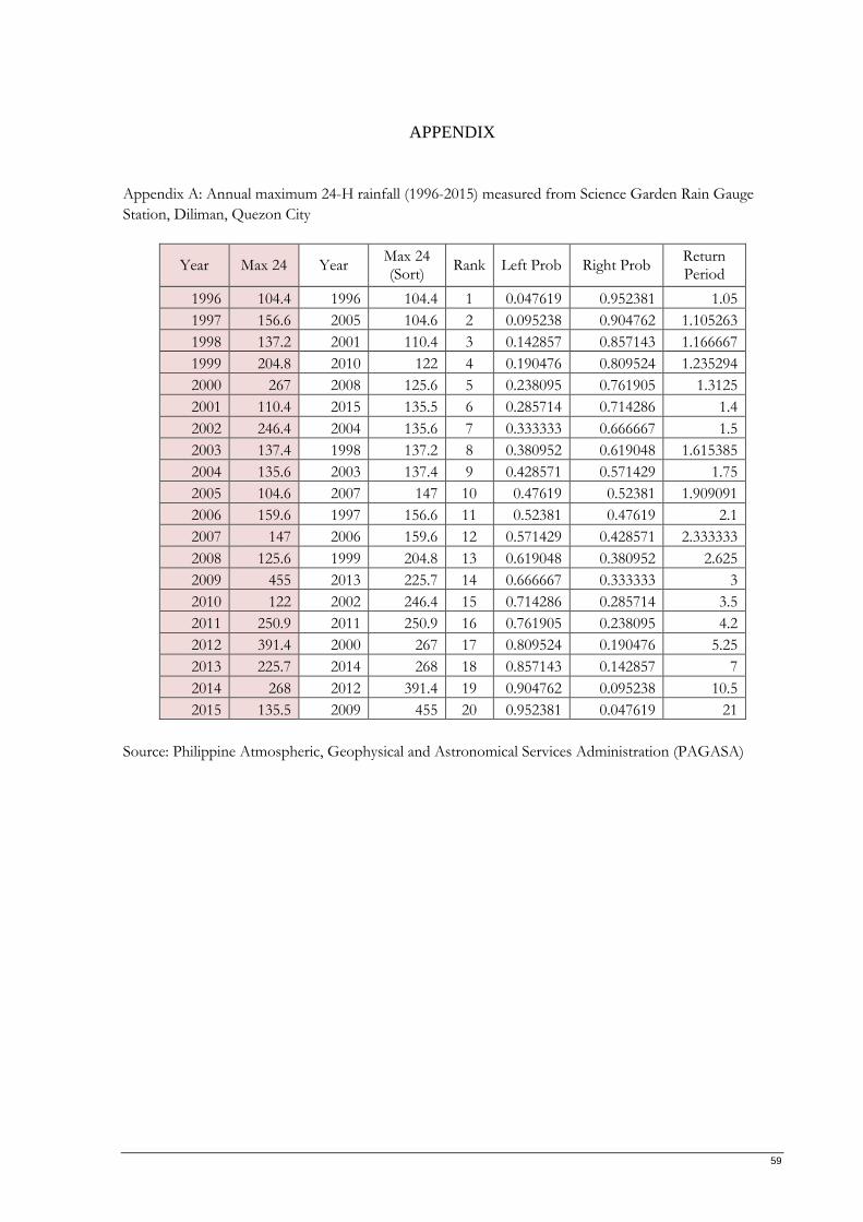
59
APPENDIX
Appendix A: Annual maximum 24-H rainfall (1996-2015) measured from Science Garden Rain Gauge
Station, Diliman, Quezon City
Year Max 24 Year Max 24 (Sort)
Rank Left Prob Right Prob Return Period
1996 104.4 1996 104.4 1 0.047619 0.952381 1.05
1997 156.6 2005 104.6 2 0.095238 0.904762 1.105263
1998 137.2 2001 110.4 3 0.142857 0.857143 1.166667
1999 204.8 2010 122 4 0.190476 0.809524 1.235294
2000 267 2008 125.6 5 0.238095 0.761905 1.3125
2001 110.4 2015 135.5 6 0.285714 0.714286 1.4
2002 246.4 2004 135.6 7 0.333333 0.666667 1.5
2003 137.4 1998 137.2 8 0.380952 0.619048 1.615385
2004 135.6 2003 137.4 9 0.428571 0.571429 1.75
2005 104.6 2007 147 10 0.47619 0.52381 1.909091
2006 159.6 1997 156.6 11 0.52381 0.47619 2.1
2007 147 2006 159.6 12 0.571429 0.428571 2.333333
2008 125.6 1999 204.8 13 0.619048 0.380952 2.625
2009 455 2013 225.7 14 0.666667 0.333333 3
2010 122 2002 246.4 15 0.714286 0.285714 3.5
2011 250.9 2011 250.9 16 0.761905 0.238095 4.2
2012 391.4 2000 267 17 0.809524 0.190476 5.25
2013 225.7 2014 268 18 0.857143 0.142857 7
2014 268 2012 391.4 19 0.904762 0.095238 10.5
2015 135.5 2009 455 20 0.952381 0.047619 21
Source: Philippine Atmospheric, Geophysical and Astronomical Services Administration (PAGASA)

60
Appendix B: Particle Size Analysis Calculation
The basis of the calculations is the oven-dry sample weight after all treatments. It is obtained by the
summation of all individual fractions:
Clay (<2 μm) = (H * 50) – (Z * 50) (wt. K)
Silt (2-20 μm) = (G * 50) – (Z * 50) – K (wt. L)
Silt (20-50 μm) = (F * 50) – (Z * 50) – K - L (wt M)
Sand (>50 μm) = A + B + C + D + E (wt N)
Sample weight = K + L + M + N *weight all in grams
Where:
A through E = weight of individual sand fractions
F = weight 20ml pipette aliquot of fraction <50 μm
G = weight 20ml pipette aliquot of fraction <20 μm
H = weight 20ml pipette aliquot of fraction <2 μm
Z = weight 20ml pipette aliquot of blank
Proportional amounts of the fractions can be calculated by:
% clay (<2 µm) = K * 100
sample wt.
% silt (2 -2 µm) = L * 100
sample wt.
% silt (20-50 µm) = M *100
sample wt.
% sand (1000-2000 µm) = A *100
sample wt.
% sand (500-1000 µm) = B *100
sample wt.
% sand (250-500 µm) = C *100
sample wt.
% sand (100-250 µm) = D *100
sample wt.
% sand (50-100 µm) = E *100
sample wt.
Source: Particle Size Analysis, ITC, Geoscience Lab.

61
Appendix C: Required input database format for OpenLisem
Variable name Data/Map name Rainfall Rainfall file
Id.map
Catchment Dem.map
Grad.map
Ldd.map
Outlet.map
Outpoint.map
Landuse LULC.map
Per.map
Lai.map
Ch.map
Roadwidt.map
Grasswid.map
Smax.map
Surface rr.map
n.map
Stonefrc.map
Crustfrc.map
Compfrc.map
Hardsurf.map
Infiltration (1st layer Green & Ampt) Ksat1.map
Psi1.map
Thetas1.map
Thetai1.map
Soildep1.map
Channels (Channel Properties) Lddchan.map
Chanwidt.map
Chanside.map
Changrad.map
Chanman.map
Chancoh.map
Channel Flood Chandepth.map
Barriers.map
Chanmaxq.map
Chanlevee.map
Hmxinit.map
Floodzone.map
Houses Housecover.map
Source: LISEM Manual version 2.x – January 2, 2002

62
Appendix D: Parameters used by Mines and Geosciences Bureau for Flood Mapping
Source: DENR – MGB Guidebook for the conduct of landslide and flood susceptibility assessment and mapping (1:10,000 scale)