of - dticfinally, the deepest expression of my thanks has to go to my fianc4, linda. her constant...
TRANSCRIPT

91 .
THE ENHANCED P~ERFORMANCE OF AN
INTEGRATED NAVIGATION SYSTEM
I4IN A IIIGIIIY I)YNAMIC ENVIRONMENT
TIIFESISBrian J. tohlenekCDC
.. . .' Second Lieutenant, UISA I1
AFIT/(,E/FNG/94 I)-0I
,for public :e"Cas ,C:"e.iSdistribýution .m ~ z:e
DEPARTMENT OF THE AIR FORCE
AIR UNIVERSITY
AIR FORCE INSTITUTE OF TECHNOLOGY
Wright-Patterson Air Force Base, Ohio

AFIT/GE/ENG/94D-O 1
r)j
A-cedC on F or.T-----.-I --- 4&. THE ENHANCED P ERFORMANCE OF AN
D-ti INTEGRATED NAVIGATION SYSTEMUr Ij IN A HIGHLY DYNAMIC ENVIRONMENT
By ---------------------------------T H E SISD~s Brian J. Boheniek
S ~ Second Lieutenant, USAF
AFIT/GE/ENG/94D-01Dt
DTIC QýfJ1% 1 ITY TLT'T
Approved for public release; distribution unlimited

The views expressed in this thesis are those of the author and do not reflect the official policy or
position of the Department of Defense or the U. S. Government.

AFIT/GE/ENG/94D-O1
THE ENHANCED PERFORMANCE OF AN INTEGRATED NAVIGATION
SYSTEM IN A HIGHLY DYNAMIC ENVIRONMENT
THESIS
Presented to the Faculty of the Graduate School of Engineering
of the Air Force Institute of Technology
Air University
In Partial Fulfillment of the
Requirements for the Degree of
Master of Science in Electrical Engineering
Brian J. Bohenek, B.S. Electrical Engineering
Second Lieutenant, USAF
December 1994
Approved for public release; distribution unlimited

Preface
The completion of this thesis is not the work of just one person but of several people who either
directly or indirectly helped make this thesis a reality. First of all, my sponsoring organization, the
Central Inertial Guidance Test Facility (CIGTF) of the 46th Test Group, Holloman AFB, NM. This
thesis was completed in support of their mission to test and evaluate the accuracy and reliability
of integrated navigation systems.
The efforts of Captain Neil Hansen, CN Air Force, in development of the PNRS models in
MSOFE which were vital in the successful completion of this thesis. I would also like to thank
1Lt William "Chip" Mosle of CIGTF who on many occasions helped me to understand the inner
workings of MSOFE which proved to be most helpful.
I would also like to thank the members of my thesis committee for their help and guidance
throughout this thesis effort. A special thanks must go out to Lt Col Robert Riggins, my thesis
advisor. His constant support and encouragement always kept me focused on where I was going
with my thesis especially when it seemed like I ran into a brick wall. I would also like to thank
Dr. Peter Maybeck for his diligence and "eagle eye" when proof-reading and evaluating my written
work. Also, thanks must go out to Captain Ron Delap for his time and effort in proof-reading and
evaluating my work along with words of encouragement.
Thanks must go out to the Guidance and Control Class of GE-94D. Their guidance and
support with class work proved to be most valuable when needed. Also to the "Tuesday and
Thursday Basketball Crew," thanks for well needed stress reliefs throughout this thesis effort. I
would especially like to thank Captain Pete Eide whose support, SEGA stress relief games, and
assistance with class work proved to invaluable for me to make it to graduation.
My family deserves a special thanks for their constant support in all that I have accomplished.
Mom, Dad, and Jason thanks for all the love and support over the years, I would not be where I
am today without you behind me.
ii

Finally, the deepest expression of my thanks has to go to my fianc4, Linda. Her constant
support, strength, love, and encouragement throughout the last year and a half always helped me
to maintain a proper perspective and focus on my thesis. She was able to put up with all of the
stress associated with medical school and would always find time for me and for this I am most
thankful.
Brian J. Bohenek
111

Table of Contents
Page
Preface ................ ............................................. ii
List of Figures ............. ......................................... viii
List of Tables .............. .......................................... xiii
Abstract .............. ............................................. xvi
I. Introduction ........... ....................................... 1-1
1.1 Background .......... ................................. 1-2
1.2 Problem Statement ........... ............................ 1-3
1.3 Summary of Previous Knowledge ............................ 1-4
1.4 Assumptions .......... ................................ 1-6
1.5 Scope ........... .................................... 1-10
1.6 Approach/Methodology .................................. 1-11
1.7 Overview of Thesis ...................................... 1-14
II. Theory .............. .......................................... 2-1
2.1 Overview ........... .................................. 2-1
2.2 Extended Kalman Filtering ................................ 2-1
2.2.1 Extended Kalman Filter Equations ...... ............... 2-1
2.2.2 Kalman Filter Order Reduction ...... ................. 2-6
2.2.3 Kalman Filter Tuning ........ ...................... 2-8
2.3 Carrier-Phase Global Positioning System Measurements ............ 2-10
2.3.1 Carrier-Phase GPS Observation Equations ............... 2-10
2.3.2 Carrier-Phase GPS Phase Range Measurement Equations . 2-13
2.3.3 Differencing Techniques ............................ 2-15
2.3.4 Cycle Slips ......... ............................ 2-22
iv

Page
2.4 Failure Detection, Isolation, and Recovery (FDIR) Scheme .......... 2-24
2.4.1 The Chi-Square Test .............................. 2-24
2.4.2 The Multiple Model Adaptive Estimator (MMAE) ...... .... 2-25
2.5 Summary .......... .................................. 2-28
III. The ENRS and PNRS Models ......... ............................. 3-1
3.1 Overview ............ .................................. 3-1
3.2 The ENRS Model .......... ............................. 3-1
3.2.1 Litton LN-93 Error State Models ...................... 3-2
3.2.2 Range/Range-Rate System Error State Model ............. 3-4
3.2.3 Differential GPS Error State Model .................... 3-11
3.3 The PNRS Model ......... ............................. 3-16
3.3.1 The PNRS Truth Model Equations .................... 3-16
3.3.2 The PNRS Measurement Equations .................... 3-18
3.4 The PNRS Double Difference Model .......................... 3-19
3.4.1 The PNRS Double Difference Error State Model ........... 3-20
3.4.2 The PNRS Double Difference Measurement Equations . . .. 3-20
3.5 The PNRS Truth and Filter Models .......................... 3-22
3.5.1 The 91-State Truth Model ........................... 3-22
3.5.2 The 19-State Filter Model ........................... 3-22
3.6 The Double Difference Truth and Filter Models .................. 3-23
3.6.1 The 89-State Double Difference Truth Model .............. 3-23
3.6.2 The 17-State Double Difference Filter Model .............. 3-23
3.6.3 The 69-State Double Difference Filter Model .............. 3-24
3.7 Other Measurements ......... ............................ 3-24
3.7.1 Barometric Altimeter Measurement ...... .............. 3-24
3.7.2 Velocity Aided Measurement ....... .................. 3-25
3.8 Summary .......... .................................. 3-26
v

Page
IV. Filter Implementation Results ......... ............................. 4-1
4.1 Overview ........... .................................. 4-1
4.2 Simulation Specifications ......... ......................... 4-1
4.3 The Removal of the Perfect Doppler Velocity Aiding ............... 4-4
4.4 The 71-State PNRS Filter without Velocity Aiding ................ 4-5
4.5 The Reduced Order PNRS Filter Results ....... ................ 4-9
4.5.1 Normal-Running Filter with Velocity Aiding ..... ......... 4-9
4.5.2 Cycle Slip Simulation Results ......................... 4-13
4.6 The Reduced Order PNRS Filter with Double Differencing .......... 4-15
4.6.1 Normal-Running Double Difference Filter ................ 4-16
4.6.2 Cycle Slip Simulation with a Double Difference Filter . . .. 4-17
4.7 FDIR Simulation Results ........ ......................... 4-21
4.7.1 FDIR Results from the ROPNRS Filter ................. 4-22
4.7.2 FDIR Results from the DDPNRS Filter ................. 4-24
4.8 Summary .......... .................................. 4-25
V. Conclusions and Recommendations ......... .......................... 5-1
5.1 Overview ........... .................................. 5-1
5.2 Conclusions .......... ................................. 5-1
5.2.1 The Removal of the Perfect Doppler Velocity Aiding Measure-
ments .......... ............................... 5-1
5.2.2 The PNRS Filter Order Reduction ..................... 5-2
5.2.3 The Implementation of Double Differencing ............... 5-2
5.2.4 The FDIR Algorithm Against Large Cycle Slips ........... 5-3
5.3 Recommendations ......... ............................. 5-3
5.3.1 Incorporation of a Realistic Doppler Velocity Model ..... 5-3
5.3.2 Implementation of the True Double Differencing of (8) . . .. 5-4
5.3.3 Investigation or Elimination of the Correlation Involved with
Double Differencing ........ ....................... 5-4
vi

Page
5.3.4 Test PNRS Filters Against Real Data ...... ............. 5-4
5.3.5 Investigation of CPGPS Measurements in MSOFE ...... .... 5-5
5.3.6 Continued Development of Proposed MMAE Algorithm . . . 5-5
Appendix A. Error State Models Definitions ........ ...................... A-1
Appendix B. Litton LN-93 INS Error State Model Dynamics and Noise Matrices B-1
Appendix C. PNRS and DDPNRS Noise Matrcies (Q(t) and R(t)) Values ..... C-1
Appendix D. 71-States PNRS Filter without Velocity Aiding Results ............. D-1
Appendix E. Reduced Order PNRS Filter Results with Velocity Aiding .......... E-1
Appendix F. Reduced Order PNRS Filter Results without Velocity Aiding ..... F-1
Appendix G. The Double Difference PNRS Filter Results .................... G-1
Appendix H. Double Difference PNRS Small Cycle Slip on Satellite #1 Results . . H-1
Appendix I. Double Difference PNRS Satellite #1 Loss Results ................ I-1
Appendix J. Double Difference PNRS Large Cycle Slip on Satellite #1 Results J-1
Appendix K. Double Difference PNRS Large Cycle Slip on Satellite #4 Results K-1
Appendix L. FDIR Results from Chi-Square Analysis ....................... L-1
L.1 Chi-Square Test from the ROPNRS Filter ...................... L-1
L.2 Chi-Square Test from the DDPNRS Filter ...................... L-7
Appendix M. Lack of Independence of GPS Satellite Differencing Proof ....... .... M-1
Bibliography .......... .......................................... BIB-1
Vita ........... ............................................... VITA-1
vii

List of Figures
Figure Page
1.1. Block Diagram of CIGTF's NRS with CPGPS ....... ................... 1-2
1.2. GPS, RRS Antenna and INS Locations on Model Test Aircraft ..... ......... 1-8
1.3. Block Diagram of CIGTFs NRS as Implemented in MSOFE ................ 1-12
1.4. NRS Implementation in MSOFE with Single Differencing Between Receiver and
Satellites ............ ........................................ 1-13
2.1. Pictorial Representation of the Total Phase-Range Measurement ............. 2-14
2.2. Illustration of CPGPS Between-Receivers Single Difference: ARij = Ri - Rj . . 2-16
2.3. Illustration of CPGPS Between-Satellites Single Difference: VR'j = Ri - Rf . . 2-18
2.4. Illustration of CPGPS Between-Time Epochs Single Difference: 6tR(ti - tj) =
R(ti) - R(tj) ............ ..................................... 2-19
2.5. Illustration of CPGPS Between Receivers/Satellites Double Difference: VARtj -
ARGBRABR -- ARJGBR,ABR .............................. 2-21
2.6. Block Diagram of MMAE Algorithm (16) ....... ..................... 2-27
2.7. Block Diagram of Proposed PNRS MMAE Algorithm .................... 2-28
2.8. Block Diagram of MMAE Algorithm with Hierarchical Structure ..... ........ 2-30
3.1. Pictorial Representation of RRS Measurements ....... .................. 3-5
3.2. Pictorial Representation of DGPS Measurements ...... ................. 3-11
4.1. Three-Dimensional Representation of Fighter Flight Profile ................. 4-2
4.2. Two-Dimensional Representation of Fighter Flight Profile ...... ............ 4-3
4.3. Three-Dimensional Representation of Fighter Flight Profile with Transponder Lo-
cations ............. ......................................... 4-5
4.4. Comparison of Vertical Velocity Error States ........ .................... 4-6
4.5. Comparison of Longitude Error States ........ ....................... 4-8
4.6. Untuned Vertical Velocity Error without Velocity Aiding .................. 4-12
viii

Figure Page
4.7. Incorrect Implementation of a Large Cycle Slip ....... .................. 4-14
4.8. Correct Implementation of a Large Cycle Slip ....... ................... 4-15
4.9. DDPNRS Filter Residuals for a Small Cycle Slip on Satellite 4 .............. 4-18
4.10. DDPNRS Phase Ambiguity Error States for a Satellite Loss Cycle Slip ..... 4-20
D.1. Longitude and Latitude Error Plots ........ ......................... D-2
D.2. Altitude and Barometric Altimeter Error Plots ....... .................. D-3
D.3. North, West, and Azimuth Tilt Error Plots ........ .................... D-4
D.4. North, West, and Vertical Velocity Error Plots .......................... D-5
D.5. RRS Range Bias, Range Velocity, and Atmospheric Propagation Delay Error Plots D-6
D.6. RRS X, Y, and Z Position Error Plots ........ ....................... D-7
D.7. GPS User Clock Bias and User Clock Drift Error Plots .................... D-8
D.8. GPS Satellites 1 and 2 Phase Ambiguity Error Plots ...... ............... D-9
D.9. GPS Satellites 3 and 4 Phase Ambiguity Error Plots .................... D-10
E.1. Longitude and Latitude Error Plots ........ ......................... E-2
E.2. Altitude and Barometric Altimeter Error Plots ...... .................. E-3
E.3. North, West, and Azimuth Tilt Error Plots ........ .................... E-4
E.4. North, West, and Vertical Velocity Error Plots .......................... E-5
E.5. RRS Range Bias and Range Velocity Error Plots ...... ................. E-6
E.6. GPS Clock Bias and Drift Error Plots ........ ....................... E-7
E.7. GPS Satellites 1 and 2 Phase Ambiguity Error Plots ...... ............... E-8
E.8. GPS Satellites 3 and 4 Phase Ambiguity Error Plots ...... ............... E-9
F.1. Longitude and Latitude Error Plots ........ ......................... F-2
F.2. Altitude and Barometric Altimeter Error Plots ....... .................. F-3
F.3. North, West, and Azimuth Tilt Error Plots ........ .................... F-4
F.4. North, West, and Vertical Velocity Error Plots .......................... F-5
F.5. RRS Range Bias and Range Velocity Error Plots ...... ................. F-6
ix

Figure Page
F.6. GPS Clock Bias and Drift Error Plots ........ ....................... F-7
F.7. GPS Satellites 1 and 2 Phase Ambiguity Error Plots ...... ............... F-8
F.8. GPS Satellites 3 and 4 Phase Ambiguity Error Plots ...... ............... F-9
G.1. Longitude and Latitude Error Plots ........ ......................... G-2
G.2. Altitude and Barometric Altimeter Error Plots ....... .................. G-3
G.3. North, West, and Azimuth Tilt Error Plots ........ .................... G-4
G.4. North, West, and Vertical Velocity Error Plots .......................... G-5
G.5. RRS Range Bias and Range Velocity Error Plots ...... ................. G-6
G.6. GPS Satellites 1 and 2 Phase Ambiguity Error Plots ...... ............... G-7
G.7. GPS Satellites 3 and 4 Phase Ambiguity Error Plots ...... ............... G-8
H.1. Longitude and Latitude Error Plots ........ ......................... H-2
H.2. Altitude and Barometric Altimeter Error Plots ....... .................. H-3
H.3. North, West, and Azimuth Tilt Error Plots ....... .................... I-4
H.4. North, West, and Vertical Velocity Error Plots .......................... H-5
H.5. RRS Range Bias, Range Velocity, and Atmospheric Propagation Delay Error Plots H-6
H.6. GPS Satellites 1 and 2 Phase Ambiguity Error Plots ...... ............... H-7
H.7. GPS Satellites 3 and 4 Phase Ambiguity Error Plots ...... ............... H-8
11.8. GPS Satellites 1 and 2 Residual Plots ................................ 1-9
H.9. GPS Satellites 3 and 4 Residual Plots ............................... H-10
1.1. Longitude and Latitude Error Plots ........ ......................... 1-2
1.2. Altitude and Barometric Altimeter Error Plots ....... .................. 1-3
1.3. North, West, and Azimuth Tilt Error Plots ........ .................... 1-4
1.4. North, West, and Vertical Velocity Error Plots ........................ . I-5
1.5. RRS Range Bias, Range Velocity, and Atmospheric Propagation Delay Error Plots 1-6
1.6. GPS Satellites 1 and 2 Phase Ambiguity Error Plots ...... ............... 1-7
1.7. GPS Satellites 3 and 4 Phase Ambiguity Error Plots .................... . I-8
x

Figure Page
1.8. GPS Satellites 1 and 2 Residual Plots ........ ........................ 1-9
1.9. GPS Satellites 3 and 4 Residual Plots ................................ 1-10
J.1. Longitude and Latitude Error Plots ........ ......................... J-2
J.2. Altitude and Barometric Altimeter Error Plots ....... .................. J-3
3.3. North, West, and Azimuth Tilt Error Plots ........ .................... J-4
3.4. North, West, and Vertical Velocity Error Plots ......................... J-5
J.5. RRS Range Bias, Range Velocity, and Atmospheric Propagation Delay Error Plots J-6
J.6. GPS Satellites 1 and 2 Phase Ambiguity Error Plots ...... ............... J-7
3.7. GPS Satellites 3 and 4 Phase Ambiguity Error Plots ...... ............... J-8
J.8. GPS Satellites 1 and 2 Residual Plots ................................ J-9
3.9. GPS Satellites 3 and 4 Residual Plots ................................ J-10
K.1. Longitude and Latitude Error Plots ........ ......................... K-2
K.2. Altitude and Barometric Altimeter Error Plots ....... .................. K-3
K.3. North, West, and Azimuth Tilt Error Plots ...... ..................... K-4
K.4. North, West, and Vertical Velocity Error Plots .......................... K-5
K.5. RRS Range Bias, Range Velocity, and Atmospheric Propagation Delay Error Plots K-6
K.6. GPS Satellites 1 and 2 Phase Ambiguity Error Plots ...... ............... K-7
K.7. GPS Satellites 3 and 4 Phase Ambiguity Error Plots ...... ............... K-8
K.8. GPS Satellites 1 and 2 Residual Plots ................................ K-9
K.9. GPS Satellites 3 and 4 Residual Plots ................................ K-10
L.1. Chi-Square Plots of Individual Residuals for Cycle Slip on Satellite #1 ..... L-2
L.2. Chi-Square Plots of Individual Residuals for Cycle Slip on Satellite #2 ..... L-3
L.3. Chi-Square Plots of Individual Residuals for Cycle Slip on Satellite #3 ..... L-4
L.4. Chi-Square Plots of Individual Residuals for Cycle Slip on Satellite #4 ..... L-5
L.5. Chi-Square Plots of Individual Residuals for Multiple Cycle Slip Scenario .... L-6
L.6. Chi-Square Plots of Individual Residuals for Cycle Slip on Satellite #1 ..... L-8
xi

Figure Page
L.7. Chi-Square Plots of Individual Residuals for Cycle Slip on Satellite #2 L-9
L.8. Chi-Square Plots of Individual Residuals for Cycle Slip on Satellite #3 L-10
L.9. Chi-Square Plots of Individual Residuals for Cycle Slip on Satellite #4 L-11
L.10. Chi-Square Plots of Individual Residuals for Multiple Cycle Slip Scenario. . . . L-12
xii

List of Tables
Table Page
2.1. CPGPS Measurement Difference Symbols ....... ..................... 2-16
2.2. Effects of CPGPS Difference Measurement Methods ...................... 2-22
4.1. RRS Transponder Transmitter Locations in the PNRS Simulations ........... 4-4
4.2. Comparison of PNRS True Filter Errors with and without Velocity Aiding . . . 4-7
4.3. Temporal Averages of True Filter Errors (lo) ...... ................... 4-10
4.4. Temporal Averages of True Filter Errors (lo) of ROPNRS Filter ............ 4-11
4.5. Temporal Averages of True Filter Errors (lo) of ROPNRS and DDPNRS Filter 4-16
4.6. Large Cycle Slip Recovery Times of Satellites 1 and 4 of the DDPNRS Filter 4-21
4.7. Multiple Cycle Slip Induction Parameters ....... ..................... 4-22
A.1. 93-state LN-93 INS Model, Category I: General Errors ...... .............. A-2
A.2. 93-state LN-93 INS Model, Category II: First Order Markov Process Error States A-3
A.3. 93-state LN-93 INS Model, Category III: Gyro Bias Error States ..... ........ A-4
A.4. 93-state LN-93 INS Model, Category IV: Accelerometer Bias Error States . . . A-4
A.5. 93-state LN-93 INS Model, Category V: Thermal Transient Error States . . .. A-5
A.6. 93-state LN-93 INS Model, Category VI: Gyro Compliance Error States . . .. A-5
A.7. 26-state RRS Error Model ......... .............................. A-6
A.8. 30-state GPS Error Model ......... .............................. A-7
A.9. 22-state DGPS Error Model ......... ............................. A-8
A.10. 4-state CPGPS Error Model ......... ............................. A-8
A.11. 91-state PNRS Truth Model: States 1-24 ........ ...................... A-9
A.12. 91-state PNRS Truth Model: States 25-43 ....... ..................... A-10
A.13. 91-state PNRS Truth Model: States 44-67 ....... ..................... A-11
A.14.91-state PNRS Truth Model: States 68-91 ....... ..................... A-12
A.15. 19-state PNRS Filter Model ......... ............................. A-13
xiii

Table Page
A.16. 89-State DDPNRS Double Difference Truth Model States 1-22 and Filter Model
States 1-22 .......... ....................................... A-14
A.17. 89-State DDPNRS Double Difference Truth Model States 23-41 and Filter Model
States 23-41 ........... ...................................... A-15
A.18. 89-State DDPNRS Double Difference Truth Model States 42-65 and Filter Model
States 42-65 ........... ...................................... A-16
A.19. 89-State DDPNRS Double Difference Truth Model States 66-89 and Filter Model
States 66-69 ........... ...................................... A-17
A.20. 17-State DDPNRS Filter Model ........ ........................... A-18
B.1. Elements of Dynamics Submatrix F11 . . . . . . .. . . . . . . . . . . . . . . . . .. . . . . . . B-2
B.2. Elements of Dynamics Submatrix F 12 . . . . . . .. . . . . . . . . . . . . . . . . .. . . . . . . B-3
B.3. Elements of Dynamics Submatrix F13. . . . . . . .. . . . . . . . . . . . . . . . . .. . . . . . . B-4
B.4. Elements of Dynamics Submatrix F 14 . . . . . . .. . . . . . . . . . . . . . . . . .. . . . . . . B-5
B.5. Elements of Dynamics Submatrix F 15 . . . . . . .. . . . . . . . . . . . . . . . . .. . . . . . . B-6
B.6. Elements of Dynamics Submatrix F 16 . . . . . . .. . . . . . . . . . . . . . . . . .. . . . . . . B-6
B.7. Elements of Dynamics Submatrix F 22 . . . . . . .. . . . . . . . . . . . . . . . . .. . . . . . . B-7
B.8. Elements of Dynamics Submatrix F 55 . . . . . . .. . . . . . . . . . . . . . . . . .. . . . . . . B-7
B.9. Elements of Process Noise Submatrix Qi .......... ..................... B-8
B.10. Elements of Process Noise Submatrix Q22 ...... ..................... .... B-8
C.1. PNRS Truth and Reduced Order Filter Model Tuning Values of Q(t) Matrix with
Velocity Aiding ........... .................................... C-2
C.2. PNRS Truth and Reduced Order Filter Model Tuning Values of Q(t) Matrix
without Velocity Aiding .......... ............................... C-3
C.3. DDPNRS Truth and Filter Model Tuning Values of Q(Q) Matrix ............. C-4
C.4. Measurement Noise Covariance Values of R(tQ) Matrix for PNRS Filter ..... C-5
C.5. Measurement Noise Covariance Values of R(t4) Matrix for DDPNRS Filter . . . C-5
D.1. Legend for Filter Tuning Plots ......... ............................ D-1
xiv

Table Page
E.1. Legend for Filter Tuning Plots ......... ............................ E-1
F.1. Legend for Filter Tuning Plots ......... ............................ F-1
G.1. Legend for Filter Tuning Plots ..................................... G-1
11.1. Legend for Filter Tuning Plots ......... ............................ H-1
1.1. Legend for Filter Tuning Plots ......... ............................ I-1
J.1. Legend for Filter Tuning Plots ......... ............................ J-1
K. 1. Legend for Filter Tuning Plots ..................................... K-1
xv

AFIT/GE/ENG/94D-01
Abstract
For the U. S. Air Force to maintain an accurate and reliable Navigation Reference System
(NRS) with Carrier-Phase Global Positioning System (CPGPS) measurements, it must develop
an accurate and robust NRS in the face of cycle slips caused by highly dynamic maneuvers. This
research investigates the implementation of a double differencing between receivers/satellites scheme
to improve the accuracy of current NRS models. The removal of the "perfect Doppler velocity aiding
measurements" (a very poor assumption of past research) was completed with stable and accurate
results. The double differencing implemented showed improvement in the accuracy of the NRS. An
investigation of two Failure Detection, Isolation, and Recovery (FDIR) algorithms for large cycle
slip failures is conducted. The two FDIR techniques are the Chi-Square test and a Multiple Model
Adaptive Estimator (MMAE). The FDIR results show that a Chi-Square test as a stand-alone
algorithm can work accurately for detection and isolation of failures with an accurate and reliable
recovery algorithm. The MMAE algorithm as conjectured seems to be the best FDIR technique to
handle single and multiple cycle slips accurately and reliably.
xvi

THE ENHANCED PERFORMANCE OF AN INTEGRATED NAVIGATION
SYSTEM IN A HIGHLY DYNAMIC ENVIRONMENT
L Introduction
The Central Inertial Guidance Test Facility (CIGTF), of the 46th Test Group, located at
Holloman AFB in New Mexico, is currently in the process of upgrading their Navigation Reference
System (NRS) to incorporate highly accurate Carrier-Phase measurements of the Global Position-
ing System (GPS). The addition of Carrier-Phase GPS measurements is expected to improve the
accuracy of the NRS to ensure that the NRS keeps an order of magnitude or better accuracy ad-
vantage over the navigation system under test. This accuracy advantage is necessary for CIGTF
to provide the Air Force with an accurate and reliable benchmark upon which to analyze the
performance of navigation systems under test.
The upgraded NRS will be composed of three different navigation systems: a Litton LN-93
Inertial Navigation System (INS), Carrier-Phase Global Positioning System (CPGPS), and the
Range/Range-Rate System (RRS) of ground transponders. The NRS is an airborne system which
optimally calculates the position and velocity errors of the test system through the use of an
Extended Kalman Filter (EKF) to correct the INS-indicated position of the aircraft. Figure 1.1
depicts the configuration of the NRS with the incorporation of CPGPS measurements.
The system under test is flown by CIGTF over the test range and measurements from the RRS
transponders, GPS receiver, and NRS INS, along with the navigation solution of the test system,
are recorded to magnetic storage devices for post-flight processing. The post-flight processing of
the data provides the NRS EKF solution, which is used in comparison with the navigation solution
of the test item.
1-1

x +6x INS Indicated User Position est EstimateINS of User States
Conversion of INS computed positioninto CPGPS and RRS Ranges
Rs
CPGPS Ranges
Rtu + 6R cGs+ 6z PSC Rue A5eps CPGPS
S-GPSEXTENDED 5x Optimal Estimate
KALMAN of INS Errors+ 6zRS FILTER
RRSR +-R"true RRS
RRS Ranges
Figure 1.1 Block Diagram of CIGTF's NRS with CPGPS
1.1 Background
The current incorporation of Differential GPS (DGPS) and RRS measurements in the NRS
has provided CIGTF with an adequate benchmark for inertial navigation system testing. Due to
the current advances in technology and the emergence of the embedded GPS/INS systems, the
accuracy levels of these new and upcoming navigation systems are beginning to approach and
possibly exceed the accuracy level of the NRS. For the NRS to continue to be considered a reliable
reference system, CIGTF must continue to upgrade the equipment and algorithms of the NRS to
improve its accuracy. The incorporation of CPGPS measurements into the NRS is the way CIGTF
has chosen to keep the accuracy of the NRS ahead of the new and upcoming systems.
The masters thesis and temporary duty assignment to CIGTF of Captain Neil Hansen of
the Canadian Forces (Air) is currently being used in the development and testing of the CIGTF
High-Accuracy Positioning System (CHAPS) which incorporates CPGPS measurements into its
navigation solution. See Figure 1.1 for a block diagram depiction of CIGTF's NRS. The goals
of this CHAPS project is to create the Sub-meter Accuracy Reference System (SARS) which will
provide overall sub-meter accuracy over 2-3 hour flight profiles with baselines of up to 300 miles
1-2

from the NRS (8). The acronym NRS will be used throughout the rest of this thesis to refer to
CHAPS and SARS, the reference system currently being used and tested by CIGTF.
To ensure the NRS can accurately evaluate an Integrated Navigation System's performance,
reducing the errors caused by high dynamics on the reference system and the implementing of a
CPGPS measurement differencing method, such as the double differencing method to be imple-
mented in this research, is the next logical step in the development of the upgraded NRS. With an
understanding of how to detect and compensate for errors associated with high dynamics, CIGTF
will continue to provide the Air Force with an accurate and reliable navigation reference system.
1.2 Problem Statement
Through the introduction of CPGPS measurements into the NRS, the overall accuracy in
the navigation solution of the reference system should be improved. In order to maintain this
high level of accuracy in all possible flight profiles, especially profiles involving highly dynamic
maneuvers, the system should be able to operate without any significant loss of accuracy in the
navigation solution. A significant cause of error in the navigation solution using CPGPS would be
"cycle slips" (For a better explanation of cycle slips, see Section 1.3 of this chapter and Chapter II,
Section 2.3.4). The capabilities of today's fighter aircraft to complete highly dynamic maneuvers
present the problem of such maneuvers causing multiple cycle slips, which over time can severely
degrade the accuracy of a navigation system such as CIGTF's NRS with CPGPS. This research
will explore the implementation of a CPGPS double differencing measurement technique to reduce
further the errors inherent in the system. Also to be covered will be the problem of cycle slips and
the development of ways to detect, isolate, and recover from the occurrence of cycle slips.
1-3

1.3 Summary of Previous Knowledge
The NRS models to be implemented in this thesis effort have come from the thesis research
of several AFIT graduate students. The thesis work of Britt Snodgrass (26), Joseph Solomon (28),
Richard Stacey (29), William Negast (23), William Mosle (20), and Neil Hansen (9) have developed
the current NRS models which are to be used in this thesis.
Neil Hansen(9) has completed the initial work in the integration of CPGPS into the current
NRS to develop the Precision Navigation Reference System (PNRS). Through a thorough investi-
gation of CPGPS characteristics, Hansen was able to construct the equations and models necessary
for implementation of CPGS into the current NRS filter. His research has shown an improvement
over the Enhanced Navigation Reference System (ENRS) results of Negast(23), who used DGPS
and not CPGPS. Although this improvement was not on the scale of an order of magnitude from
the ENRS, this- improvement validates that incorporation of CPGPS into the NRS should increase
the accuracy of the system, as expected. Hansen also investigated the effects of small and large
cycle slips (loss of phase lock between receiver and satellite) on the filter. These two types of cycle
slips were used because, through experience, it was found that these are the most realistic types of
cycle slips (9). The results from these tests showed that the effects of small cycle slips can become
"lost in the noise" and never become observable in the navigation solution (9). For large cycle slips,
the filter was able to estimate the phase ambiguity term (to be explained in Chapter II, Section
2.3.2 and apply corrections to the navigation solution with nominal errors, but the several minutes
needed for recovery is unacceptable for accurate navigation in a highly dynamic environment. Also,
Hansen did not implement any measurement differencing techniques, nor did he develop any de-
tection, isolation or recovery algorithms in his evaluation of cycle slips. His research concentrated
on the effects of cycle slips on the estimated variables.
The desire of CIGTF to operate an airborne sub-meter accuracy reference system over large
baselines of up to 300 miles (8) with various amounts of dynamics motivates the need to investigate
1-4

the accuracy of CPGPS systems in this type of environment. Lachapelle and his colleagues have
conducted dynamic land experiments to investigate the use of DGPS over a baseline of 600 miles
using both pseudorange and carrier-phase measurements (7). The conditions of the tests conducted
by Lachapelle et. al are similar to those experienced in a CIGTF flight test, therefore validating
its use in this research. The authors used a series of static and dynamic experiments to establish
the validity of the claim that the use of CPGPS measurements will increase the overall accuracy
of the system through the reduction of inherent errors in the system by using the more accurate
CPGPS measurements. The comparison of results of the static and dynamic experiments shows
that CPGPS measurement incorporation does increase the accuracy of the system by a margin of
one to eight meters with the use of CPGPS.
The method in which CPGPS measurements are taken has a profound effect on the overall
improvement of the accuracy of the navigation solution. Through the use of various methods of
single, double, or triple differencing between the different measurements, several significant inherent
errors of GPS can be eliminated or reduced significantly. Lachapelle, Gerard, and Casey have
investigated the use of single and double differencing techniques in high precision GPS navigation
(6). The effect each differencing technique has on inherent GPS errors was also covered in (6). An
in-depth discussion on the differencing techniques mentioned above and their effects on GPS errors
is given in Chapter II, Section 2.3.3.
The accurate estimation of the carrier-phase ambiguity term, the integer quantity from which
the CPGPS phase-range measurement is obtained, is important to the overall accuracy of the
CPGPS navigation solution in the presence of cycle slips. Because the phase ambiguities remain
unchanged until a cycle slip occurs, the phase ambiguities can, in principle, be held fixed for that
sequence once initially found (7). Interruptions of the receiver's phase monitoring, caused by highly
dynamic maneuvers or satellite shadowing due to surrounding terrain, cause the phase cycle count
to stop and cause phase cycles to be "slipped" and go uncounted. Once the receiver regains satellite
1-5

lock, the cycle slip terminates, and the receiver will begin counting cycles again as if the cycle slip
had never occurred, creating a navigation solution containing unacceptable errors. To correct for
this problem, the appropriate number of slipped cycles must be determined through estimation
using other measurements and added to all of the phase ambiguity terms affected by the cycle slip
to reestablish the original phase ambiguity (13). For more information into carrier-phase ambiguity
estimation and cycle slip occurrence, see Chapter II, Sections 2.3.2 and 2.3.4, respectively.
If a cycle slip does occur, it must be compensated, as stated previously, otherwise the CPGPS
receiver will provide inaccurate position readings which is unacceptable for CIGTF's upgraded NRS.
To accomplish this task, a cycle slip must first be detected, then the satellite or satellites which
have lost lock on the receiver must be determined. Once the cycle slip is detected and successfully
isolated, an algorithm to estimate the phase ambiguity term must be implemented to allow for
recovery from the cycle slip without significant degradation of the navigation solution's accuracy.
The thesis research of William Mosle (20) investigated ways of implementing failure detection,
isolation, and recovery algorithms into the NRS. Using statistical tests such as Chi-Squared and
Generalized Likelihood Ratios, Mosle was able to detect a series of different failures in the RRS
transponders and with code-phase GPS measurements successfully and recover from them. Wong
et. al in (32) discuss the importance of cycle slip removal in a GPS-INS system for high accuracy
positioning. They suggest using a Kalman filter to estimate the number of cycles slipped by keeping
track of the rate of change of the carrier phase (32). Another method of cycle slip removal can be
accomplished by using INS aiding to provide position and velocity data to the receiver to maintain
accuracy of the CPGPS measurements over the cycle slip period (11,32).
1.4 Assumptions
This section list the assumptions to be used in this thesis research. These assumptions are
clearly defined to aid the reader in making a proper evaluation of the work presented in this thesis.
1-6

1. The results presented in this thesis come from computer simulations. The truth models used
in this research are to represent the "real world." For a clear definition of all truth and filter
models implemented in this research, see Chapter III and Appendix A for a tabular listing of
the specific states.
2. The truth models developed for the Multimode Simulation for Optimal Filter Evaluation
(MSOFE)(3) used by Hansen (9) will be taken as accurate and sufficient representations of
the "real world."
3. The filter model to be used will be the reduced-order filter model of Mosle's research (20)
with the addition of four phase ambiguity states necessary for the implementation of CPGPS
measurements.
4. The one-state baro-altimeter model used in Hansen's research (9) will be assumed to be
an accurate representation of a real barometric altimeter. The use of a baro-altimeter as
an outside source of stabilization for the INS is necessary to compensate for the inherent
instability of the INS in the vertical channel (1). A description of the baro-altimeter model
can be found in Chapter II, Section 3.7.1.
5. The CPGPS antenna to be used will be placed on the top of the test aircraft's body to permit
maximum exposure of the antenna to the GPS satellite constellation. The RRS transponder
antenna will be placed on the belly of the test aircraft, again to maximize the exposure of
the antenna to the ground transponders. The two antennas will be assumed collocated at the
aircraft's center of gravity with the INS. This assumption is made to eliminate the need for
moment arm compensation in the measurements. Extensions to this research to include non-
collocated units can easily be made. Figure 1.2 depicts the locations of the INS and antennas
on a model of a typical aircraft. The locations of the antenna on the top and bottom of the
aircraft's fuselage are consistent with the locations on the test aircraft used by CIGTF. The
1-7

GPS Antenna
RRS Antenna
Figure 1.2 GPS, RRS Antenna and INS Locations on Model Test Aircraft
assumption of collocation of the INS and antennas does not hold true for CIGTF test aircraft
and is for simulation purposes only.
6. The CPGPS measurements used as inputs to the EKF implemented in MSOFE are assumed to
be differentially corrected upon entering the simulation. The noise levels associated with the
measurements are determined by the simulation's operator for implementation into MSOFE.
These adjustable noise levels allow for the simulation to represent not only one receiver but
many different receivers through proper alterations made to the input data.
7. The simulation runs to be conducted on MSOFE will be the results of 15-run Monte Carlo
analyses. Although a larger number of Monte Carlo runs would produce sample statistics
that more closely reflect the true underlying error statistics, with an infinite number of runs
producing truly optimal results, fifteen was decided upon to keep the computational burden
and time of each simulation run within reasonable limits to maximize the amount of time
devoted to true research.
8. The flight profiles and GPS satellite data used in this thesis effort will come from one of
two sources. The first source is PROFGEN and the MSOFE user subroutines ORBITS and
CALDOP. PROFGEN (22) is a software package which generates flight profile data based
on user inputs for implementation in MSOFE. The user subroutines ORBITS and CALDOP
1-8

are the results of the thesis work of Hansen and Mosle (9, 20). ORBITS calculates the
GPS satellites positions based upon GPS almanac data which is an input to the subroutine.
CALDOP determines which satellites are in view of the GPS antenna and receiver and also
calculates the Position Dilution of Precision (PDOP) for a given set of satellites which are in
view. The calculated PDOP is then compared to an operator-set maximum MAXDOP, and if
the calculated PDOP is less than MAXDOP the set of satellites is taken into the simulation.
If the PDOP is greater than MAXDOP, then CALDOP chooses another set of satellites in
view and tests the calculated PDOP until it is less than MAXDOP. The orbital trajectories
calculated by ORBITS are assumed to be correct through extensive testing and verification
completed during their development (21).
9. The Kalman filter simulation package to be used will be the established software package
MSOFE (3). All filter simulations will be run on MSOFE. All Failure Detection, Isolation,
and Recovery (FDIR) algorithms will be run on the commercial software package MATLAB
(14).
10. The differencing method to be used by CIGTF is tentatively to be a true double differenc-
ing method between receivers and satellites (10, 27). After discussion with Captain Britt
Snodgrass of CIGTF (27), it was decided to implement the double differencing method with
differentially corrected CPGPS measurements, or Method I from (8). This decision was made
because it would take a lesser amount of MSOFE recoding to be fully implemented. The time
saved in the use of this method allows for more time to be devoted to MSOFE debugging,
research, and simulation runs. Insofar as error reduction capabilities of the two different
methods mentioned, they are considered to be equivalent (25).
11. The configuration of the NRS in simulation is of a feedforward design. This configuration
does not allow for any real-time corrections to be fed back to the INS, as can be found in a
feedback configuration.
1-9

12. The double differencing method implemented will use the following satellite (SV) combina-
tions: SVl - SV4, SV2 - SV4, and SV3 - SV4 with satellite four, SV4, being arbitrarily
chosen as the base satellite. All satellite measurements are assumed independent of each
other. This allows for all process and measurement noise matrices to be diagonal (30). Ap-
pendix M contains the proof of the lack of independence of the four satellite measurements.
The independence assumption is made with full knowledge of the actual dependence of the
satellite measurements, which totally neglects the correlation between the satellites measure-
ments. To compensate for this dependence would involve significant recoding of MSOFE and
is beyond the scope of this thesis.
1.5 Scope
This thesis will concentrate on investigating the effect highly dynamic maneuvers have on
the CPGPS measurements of the NRS, and on the detection, isolation, and recovery from poor
performance. Cycle slips caused by such maneuvers will be the focus of this investigation. Of
the possible different problems faced by an integrated navigation system using CPGPS in a highly
dynamic environment, cycle slips have been determined to be the most significant. This decision
corresponds with CIGTF's main concern in highly dynamic environments.
Once the problem of cycle slip detection is conquered, the task of developing cycle slip isolation
and recovery algorithms must be completed. These algorithms are necessary to ensure that the
accuracy of the NRS stays within established tolerances during the entire flight profile, regardless
of the level of dynamics of the maneuvers of the test aircraft.
The inclusion of another CPGPS measurement technique will also be explored. The use of
a double differencing method between receivers and satellites will be implemented to improve the
accuracy of the simulated system. A double differencing technique has not been implemented at
1-10

AFIT nor CIGTF before, but is necessary to reduce/eliminate inherent errors such as the user and
satellite clock biases, atmospheric delays, and the integer phase ambiguity term.
1.6 Approach/Methodology
This research will generate accurate and reliable truth and filter error state models for an
Integrated Navigation System in a highly dynamic environments. The phenomenon of cycles slips
in the CPGPS measurements will be the concentration of this research. The study of cycle slips
will include the development of failure detection, isolation, and recovery algorithms to ensure the
accuracy of the Integrated Navigation System will not be significantly degraded during cycle slip
occurrences. The following steps will be taken to complete the stated task:
1. Hansen's 71-state filter model (9) will be reduced to 19-states (the first 15 states being Mosle's
reduced order filter (20) and the remaining four being the four CPGPS phase ambiguity
states). This filter order reduction is being accomplished to reduce the time necessary to
complete a simulation run from over two days experienced by Hansen (9) to approximately
eight hours for a full two-hour flight profile simulation run. This step will mean that retuning
of the filter will have to be completed to ensure that the accuracy of this filter will be compa-
rable to Hansen's filter. It is understood that the implementation of a reduced order filter will
never exactly reproduce the results of Hansen's work, but the retuning to be accomplished
will be to compensate for the order reduction and accuracy improvement.
2. The double differencing between receivers and satellites technique described in (8) will be
implemented. This technique is expected to increase the accuracies of the reduced order filter
through exploitation of the high accuracies attainable in CPGPS usage. This step will further
reduce the order of the filter to 17 states and reduce the order of the truth model to 89 states.
This will eliminate one of the most dominant GPS errors, the user clock bias. For a more
1-11

detailed description of the differencing techniques of CPGPS and the method to be used in
this research, see Chapter II, Section 2.3.3, Chapter III, Section 3.4.2 or (8).
3. Begin development and implementation of Cycle Slip Failure Detection, Isolation, and Recov-
ery (FDIR) algorithms. After tuning and cycle slip induction into the simulation is working
accurately and reliably, the feasibility of proposed FDIR algorithms will be studied for their
accuracy and reliability.
The NRS configuration implemented in MSOFE is depicted in Figure 1.3. When compared
to Figure 1.1, the differences between the real system and simulated system of this figure are
evident through the additions of the PROFGEN and ORBIT data blocks for flight and satellite
trajectories. Also, the real components of the NRS, the INS, GPS and RRS receivers, are replaced
by models of each component which add the modeled errors of each component to the true position
or range provided by PROFGEN or ORBITS. As can be seen in the block diagram, most of the data
INS Computed INSError States + X + 6XIN+A
x
Conversion of INS position intoPRFgue CPGTtPS and RRS Ranges
Profile Data [ 7 RN
Compute~d ýGPS >
pc i Measurements of the EXTENDED KASatellite R KALMAN
Computed RRS - R
MeasurementsI
Figure 1.3 Block Diagram of CIGTFs NRS as Implemented in MSOFE
processing is completed outside of the Extended Kalman Filter (EKF). Before any measurements
are input into the EKF, the differences between the INS-computed ranges to the GPS satellites
1-12

and RRS transponders must be subtracted from the GPS satellite and RRS transponder-computed
ranges to produce the proper error measurement for the EKF. All computations of satellite and
transponder positions and ranges are internally computed in MSOFE, while the user position comes
from the flight profile generated by PROFGEN. The outputs of the EKF are the filter's best estimate
of the INS and GPS error states.
When the double differencing technique is introduced into MSOFE, some changes must be
made to Figure 1.3. These changes are depicted in Figure 1.4. The major difference in the two
5xINS Computed INE r ror States +x + 6 x ISX +sA
x
PROFGEN Flight+Profil Data Conversion of INS
Profle Dta lposition into RRS Ranges
Differencing of INS computed
ranges between SV's i andjj z
iV R ni s+ '
SComputed RlRS z RRs INS
Measurements EXENEDA
-- •~ CVmIte GP+v°eaueet FILTER
Differencing of GPS ranges CPGPS ij
Orbit between SV's i and j
Figure 1.4 NRS Implementation in MSOFE with Single Differencing Between Receiver and Satel-lites
configurations comes in the addition of the two blocks (blocks 1 and 2) which compute the necessary
difference between satellites for the double differencing technique. The rest of the implementation
is the same as in the previous configuration of Figure 1.3.
1-13

1.7 Overview of Thesis
The methodology presented in this chapter is meant to accomplish several goals. The first
goal to be accomplished is to speed up the simulation time of the MSOFE runs without sacrificing
accuracy. Once this is accomplished, a new measurement technique will be implemented, with the
expectation that the accuracy of the system will be increased. Finally, FDIR algorithms will be
developed to preserve the system's accuracy in the face of cycle slips brought on by highly dynamic
maneuvers.
This thesis consists of five chapters. Chapter I has presented the problem to be solved and
the approach to be taken in solving it. Chapter II covers the theory involved in this thesis. Topics
covered in Chapter II include an overview of Extended Kalman Filter Theory along with Kalman
Filter tuning and filter order reduction techniques. The theory involved with Carrier-Phase GPS
includes how the measurement equations are derived, the different differencing techniques, and cycle
slips. Finally, the theory of the FDIR techniques and methods implemented will also be covered.
Chapter III presents the NRS and PNRS truth, filter, and measurement models implemented in
this thesis. The results of the filter simulations are presented in Chapter IV and Chapter V gives
conclusions and recommendations for future research.
1-14

I. Theory
2.1 Overview
The purpose of this chapter is to provide an overview of the theory involved with the Extended
Kalman Filter, Carrier-Phase GPS and proposed FDIR schemes. The Extended Kalman Filter
section will provide an overview of the equations used along with a brief discussion of filter order
reduction and filter tuning. For the Carrier-Phase GPS section, the theory associated with Carrier-
Phase GPS and the associated measurement equations are presented. A detailed explanation of the
derivation of the carrier-phase observation equations is also presented. The FDIR section includes
theoretical descriptions of the two schemes presented.
For readers unfamiliar with the topics of Extended Kalman Filtering, a review of Maybeck's
textbooks (15-17) or other texts on stochastic estimation and control is recommended. Complete
derivations and discussions of the noted topics can be found in references (15-17) from which much
of the information on Extended Kalman Filters was taken. For more information on Carrier-Phase
GPS theory, it is recommended to review (2) and (9), where much of the presented information
can be found.
2.2 Extended Kalman Filtering
2.2.1 Extended Kalman Filter Equations. The error state models of the GPS and INS
consist of a set of nonlinear state-space differential equations. These nonlinearities eliminate the
use of a Linear Kalman Filter. Because of this constraint, an EKF is to be implemented in this
thesis. The basic idea of the EKF is to relinearize about each state estimate, i(tt), once it has
been computed (16). The subsequent derivation and many of the following equations are taken
from (16).
2-1

Assume the state models are a set of non-linear continuous-time differential equations of the
form:
i(t) = fix(t),t] + G(flw(t) (2.1)
where f[x(t), t] is the state dynamics vector which in general is a nonlinear function of the state
vector x(t) and of time t. G(t) is a noise distribution matrix which is assumed for this work to be
an identity (I) matrix. The vector represented by w(t) is a white Gaussian noise process with the
following statistics:
m, = E{w()} = 0 (2.2)
and the noise strength, Q(t):
E{w(t)w T (t + r)} = Q(t)6(r) (2.3)
It is also assumed that the measurements of the system are discrete-time measurement updates
of the form:
fz(t i) = h [x( ti),t i] + v(ti) (2.4)
where z(ti) is the measurement update at time ti, h is a known vector which is a function of the
states and time. The vector h can be either linear or nonlinear. For this thesis, h is a nonlinear
function of the state vector and time due to the nonlinear nature of the GPS measurements. The
vector v(ti) represents a white Gaussian noise process with the following statistics:
m,= Ev(ti)} -= 0 (2.5)
with noise covariance, R(ti):
E {v(t,)vT(t)} =I R(ti) t = tj26)
0 tio 1
2-2

For the EKF to produce an optimal estimate of the error state vector xc(t), the system
must first be linearized. To form the linearized perturbation equations, the linearization method
described in (15) will be used. The following derivation is the linearization of Equations (2.1) and
(2.4) using this method.
First a nominal state trajectory, xn(t), is assumed to exist for all time t E T, where T
represents the complete time set under consideration, which satisfies the differential equation:
xQ(t) f[x.(), t] (2.7)
which starts from the initial condition x, (t,) = xn, where f[.,.] is the same as defined in Equation
(2.1). The nominal noise-free measurement update equation taken with respect to this nominal
trajectory becomes:
z,(ti) = h[x,(t),ti] (2.8)
where h[.,-] is as given in (2.4).
To perturb the actual state from this assumed nominal state trajectory, subtract Equation
(2.7) from (2.1):
ix(t) - ix (t)] = fx(t), t] - f[x'(t), t] + G(t)w(t) (2.9)
Now, taking a Taylor series expansion about x,, (t) on f[x(t), t] produces:
f x(t), t] = f[x(t), t] + , t! [x(t) - x, (t)] + h.o.t. (2.10)
where h.o.t. represents higher order terms which are terms of tx(t) in powers greater than one.
Now, by rearranging Equation (2.10) the following relation is produced:
f[x(t), t] - f[xM(t), t] -fx [xQ) - x.(t)] + h.o.t. (2.11)ax
2xx-(t)
2-3

which now can be substituted into Equation (2.9) to produce:
[il(t) - (01 = of[x, t] [x(t) - xn(t)] + h.o.t. + G(t)w(t) (2.12)
where 6x(t) will be used to represent [x(t) - x,.(t)]. Invoking a first order approximation and
substituting Equation (2.12) into Equation (2.9) produces:
6x(t) = F[t; x,(t)]6x(t) + G(t)w(t) (2.13)
where 5k(t) is the perturbation state derivative defined by [I(t) - ic(t)] and the matrix F[t; x, (t)]
is defined by:
F it; x. (t)] - Afix(t), t] (2.14)
Using the same procedure on Equation (2.4), the perturbed discrete-time measurement equa-
tion is expressed as:
5z(ti) = H[ti; x,(ti)]6x(ti) + v(ti) (2.15)
where the matrix H[ti; x,(ti)] is defined by:
H[t;x.(t)] = ah[x(Q), ti] (2.16)ax
H~ti;x,•(t)] - x xx,~(t,)
The nonlinear dynamics and measurement update equations have been linearized to form
"perturbation" or "error" state equations. This linearization process allows for the application of
a linearized Kalman Filter for the system described by Equations (2.13) and (2.15). The filter
implemented will output the optimal estimate of the state error vector bx represented by &x. The
estimate of the total state of the system, R(t), can be computed using:
(t) = X,(t)++ (2.17)
2-4

The preceding derivation is adequate so long as the "true" and nominal trajectories do not
differ significantly, else large unacceptable errors will result, i.e., bx(t) gets large and the higher
order terms of the Taylor series can no longer be neglected. This requirement is clearly unreasonable
for most navigation scenarios. To avoid the need for a predetermined nominal trajectory, an EKF
is to be used in this application. The EKF relinearizes about each new state estimate, i(tt), once
it has been computed. This redeclaration of the states about the new nominal trajectory ensures
that the deviations from the nominal trajectory will remain small. This validates the assumption
made earlier and allows for linear perturbation techniques to be employed with adequate results.
The state estimate and covariance are propagated from time ti to the next sample time ti+l
through the integration of the following equations:
x(t/ti) = f[•R(t/ti), t] (2.18)
P(tlti) = F[t; R(t/ti)]P(t/ti) + P(t/ti)F T[t; R(t/ti)] + G(t)Q(t)G T(t) (2.19)
where:of[x,1] (.0
F[t;i(t/ti)]- = [xt (2.20)
using the results of the previous measurement update cycle as initial conditions:
i(t/ti) = i(tQ ) (2.21)
P(ti/ti) = P(t) (2.22)
where the notation (t/ti) stands for "at time, t, based on measurements up through time ti.
2-5

With the incorporation of discrete-time measurements, zi, the EKF is accomplished through
the following equations:
K(ti) = P(t )H T [t,; i(tf)]{H[ti;i(ti )]P(t[)HT [ti; R(t7)] + R(ti)}- 1 (2.23)
i(tt) = i(t-) + K(ti){zi - h[i(t-), ti]} (2.24)
P(t+) = P(t-) - K(ti)H[ti; x(t-)]P(t•-) (2.25)
The EKF Equations (2.18) through (2.25) are programmed into MSOFE (3) for the simula-
tion.
2.2.2 Kalman Filter Order Reduction. Filter order reduction is an important step in
any filter design. Filter order reduction is the design step in which less dominant states of the
models are either eliminated, due to lack of contribution to the overall solution, or absorbed into
other more dominant states. Often implementation of a full order filter or truth model becomes
too computationally burdensome for most computer systems due to the large number of states
which must be evaluated. For example, most aircraft's computer systems have several functions
which must run simultaneously. To be able to do this on-line and in real time, the different
functions are ranked by the importance each function has in keeping the aircraft operating in a
stable environment. With this type of system, navigation filters, which are not as crucial as flight
control functions, are given lesser priority, computation time, and memory storage allocation. For
an on-line navigation filter to be able to complete its job in the time allowed, the number of states in
the filter model must be at a minimum. Otherwise, accurate measurement updates can be delayed
because the computational time for the filter can be longer than the time allotted to the filter.
This will cause the filter to have to wait until the next time computations can be made so as to
finish a run and update the states. This justifies the need for filter order reduction. Although
2-6

filter order reduction reduces the computational time of the filter, the order reduction forces the
filter to be sub-optimal as compared to full order or truth models. To compensate for this sub-
optimality problem, a process of filter tuning must be completed. Filter tuning is discussed later
in Section 2.2.3.
The models used in this thesis are the results of the previous research of Hansen (9) and
Mosle (20). Their work implemented the models of Negast (23) and his predecessors (26,28,29,31).
The LN-93 model implemented reduces the 93-state error model (5) to 39 states. This reduction
comes from the research of Lewantowicz and Keen and can found in (12). In (12), the authors
tested reduced-order models ranging from forty-one to seventeen states. The GPS and RRS models
implemented are the results of the masters' theses work of (26, 28, 29). The CPGPS models used
in this research come from (9). For a more detailed description of the INS, RRS, DPGPS, and
CPGPS models, see Chapter III.
In Hansen's research (9), a post-processing technique was adopted, as required by CIGTF.
CIGTF requires that the filter order be seventy states or less to ensure that a twenty-four hour
processing time is kept. This is based on the usage of a Hewlett-Packard 9000 minicomputer running
a ten-run Monte Carlo simulation for a two-hour aircraft flight profile (9). For this research a post-
processing technique will also be adopted. To reduce the time required to conduct a fifteen-run
Monte Carlo simulation from Hansen's research of over two days (9), the reduced order model of
Mosle's research (20) will be implemented with the addition of four phase ambiguity states necessary
for CPGPS implementation. The use of Mosle's models reduces the number of filter model states
from the seventy-one of Hansen's research to nineteen states. A more detailed description of the
models implemented in this research is given in Chapter III.
The goal of filter order reduction is to decrease the number of states of the filter model
without significant reduction in the accuracy of the state estimates from the full order or truth
2-7

model's evaluation. This makes the process of choosing which states to eliminate or combine with
other states a critical process in the design and implementation of this type of system.
2.2.3 Kalman Filter Tuning. A Kalman Filter proves to be an optimal estimator of a sys-
tem implementing dynamics and measurement equations which can be described as linear systems
driven by white Gaussian noise and deterministic inputs (15). The construction of a full order filter
model requires dynamics and measurement equations along with process and measurement noise
strengths between the filter and truth models to be identical. The process of filter order reduction
(discussed in Section 2.2.2) causes the filter-assumed process and measurement noise strengths to
be adjusted to compensate for the states which were affected in the filter order reduction. For
the Extended Kalman Filter implemented in this research, even a full order filter would not be
optimal due to the first order perturbation approximations made in deriving the Extended Kalman
Filter equations of Section 2.2.1. This process of adjusting noise strengths for model mismatching
of states is call Kalman filter "tuning." This section presents an overview of the rationale of the
tuning process used in this research.
The tuning process involves the adjustment of the values in this process noise strength matrix
Q and the measurement noise covariance matrix R. The tuning of these values continues until the
filter performance tracks the truth models to within acceptable limits. Due to the sub-optimality
of the system being implemented, the desired accuracy attained by tuning depends on the type of
application and the design engineer's discretion. For the reduction of the filter model from a full
order to some desired number of states, the filter-assumed Q and R values will in most cases be
increased except for special cases where a decrease of the Q and R terms will be necessary. An
example of a special case would be where the Qd(t4) and R(ti) values are representative at one
sample period and if the sample time is decreased the amount of uncertainty in the models and
measurements could also be decreased because the error propagation time is now shorter.
2-8

The tuning of Q takes place for three reasons. Keeping any value of the Kalman Filter gain,
K(ti), from going to zero is the first reason behind Kalman Filter tuning. The occurrence of this
problem causes the filter to become too confident in its dynamics model and to disregard totally
the information of its incoming measurements. This causes the states for which the gain value
equals zero to remain constant at the previous value and with no new measurement information
being incorporated. This is evident in Equations (2.24) and (2.25). If K(ti) = 0 then Equations
(2.24) and (2.25) become:
S= (qt) (2.26)
P(tt (t) (2.27)
showing that no new information is used in a measurement update. By increasing the Q matrix
values and decreasing the filter's confidence in its dynamics model, the K matrix can be guaranteed
to never go to zero, therefore allowing new measurement information to always be used. Another
problem to guard against involves the non-updating of individual states which is caused by indi-
vidual elements of the of the K matrix becoming zero as well as the entire K matrix becoming
zero.
The tuning of the Q values also prevents the filter covariance matrix P eigenvalues from
becoming negative. This problem is rooted in the numerical and computational accuracy of the
computer algorithms being used to run the filter simulations. This usually occurs when the range
between computed numbers is quite large or the size of the number is beyond the numerical accuracy
of the computer (for example having states with values on the order of 10+10 and other states having
values on the order of 10-10). In these two cases, a computer will often say that one or both of
the values associated with significant differences in magnitude are zero. Through increasing the Q
values, the eigenvalues can stay positive without significantly degrading the filter's performance or
accuracy.
2-9

The third reason for Q value tuning is for compensation needed for states eliminated or ab-
sorbed in filter order reduction or for the nonlinear effects ignored in the first order approximation
methods used. The states remaining after a filter order reduction which are dependent on those
states either eliminated or absorbed must be compensated for these "missing" states. The nonlinear
effects approximated in the implementation of an Extended Kalman Filter must also receive com-
pensation. This compensation comes in the form of increasing Q on those states affected directly
by filter order reduction or through relinearization.
The tuning of the measurement noise matrix R is necessary because of filter order reduction
and nonlinearity compensation. Like with the tuning of Q values for filter order reduction, the
R values associated with the states which are dependent on the states which were eliminated or
absorbed must be increased to compensate for these changes to the model. Also where linearization
of the measurement equation is needed for implementation into a linear Kalman Filter, R tuning
is used to compensate for these nonlinear effects.
The Kalman filter tuning process is by far the most time consuming portion of any design.
The tuning of Q and R must be done iteratively and with good engineering insight in order to be
successful.
2.3 Carrier-Phase Global Positioning System Measurements
2.3.1 Carrier-Phase GPS Observation Equations. A carrier-phase measurement is the
result of subtracting the generated carrier signal of the receiver from the carrier signal transmitted
by the GPS satellite being received by the receiver. This subtraction or beating of the two signals
leads to finding the phase-range, or the satellite-to-user range based on the carrier-phase. The
phase-range term is synonymous with pseudorange which is used in code-phase measurements.
The result of this subtraction step is called the carrier beat phase observable. This process is
2-10

represented by the following equation:
S= I (T) - 4 (t) (2.28)
where 4 represents the carrier beat phase observable at the receiver, k (T) represents the phase of
the carrier transmitted from the kth satellite at time T and received at time, t, and bi(t) represents
the phase of the carrier at the ith receiver at the reference signal time, t. Note: T represents the
satellite clock time of transmission while t is the receiver clock time of reception of the signal, and
throughout the rest of this thesis the i and k indicators will be dropped and the different 4 terms
will be identified by the time variable, T or t for the satellite or receiver carrier phase respectively.
The time of travel of the signal 6t is:
Rt = t - T (2.29)
By rearranging Equation (2.29), we can form:
4(t) = i(T + (2.30)
Next expand Equation (2.30) about T in a Taylor series expansion (see Equation (2.12)) produces:
eA(r) • t + h.o.i. (2.31)4D(T + 6t) = 4P(T) + a•(T R=T hot.(.1
ar ý=T
where the first derivative of $(T) with respect to time equals the frequency, f. Due to the GPS
phase/frequency relationship which is valid for highly stable oscillators over a short time interval
(such as St), the h.o.t. or higher order terms of Equation (2.31) are considered negligible. Equation
(2.31) with the frequency taken as a constant becomes:
$(T + SR) = $(T) + f . St (2.32)
2-11

Substituting Equation (2.29) into Equation (2.32) and noting that P(T + 6t) = $P(t) and 4(T) =
V9 (T), Equation (2.32) becomes:
0,(t) = Ok (T) + . (t - T) (2.33)
which can be rearranged to form:
S= k(T) - O(t= -f. (t - T) (2.34)
Now to obtain a relation of the transmission and reception times, T and t respectively, we note
the clocks of the satellite and receiver are independent of each other. Not only are these clocks
independent of each other, but each one is offset from true GPS time by some small error. If we
are to represent true GPS time as tGPS, then the reception time in relation to true GPS time is:
tGPS = t + dt (2.35)
where dt represents the user clock offset from true GPS time. Like with the reception time, the
transmission time, T, can be related to true GPS time by its own offset term, dT, plus the time
it takes for the GPS signal to propagate between the satellite and receiver. The propagation time
is the distance traveled plus errors (true range to the satellite plus ionospheric and tropospheric
errors) divided by the speed of the signal (speed of light). This relation is represented by the
following expression:
Tpropagation = (p - dion + dtrop) (2.36)C
where p is the true range between the satellite and receiver, dion is the range equivalent of the
ionospheric delay, and dtrop is the range equivalent of the tropospheric delay. The minus sign
associated with the ionospheric delay term is due to the fact that the ionosphere actually advances
2-12

the phase of the carrier signal, making it appear as if the signal travels faster than the speed of light
(9). The relation between the transmission time of Equation (2.36) and true GPS time is presented
in the following equation:
tGPS = T + dT + (p - di,, + dtrop) (2.37)C
By setting Equations (2.35) and (2.37) equal to each other, the relation between the transmission
time and reception time is:
T + dT + (p - dion + dtrop) = t + dt (2.38)C
Rearranging Equation (2.38), the following is obtained:
t - T = dT - dt + (p - dion + dtrop) (2.39)c
The carrier phase observation equation is now obtained through substituting Equation (2.39) into
Equation (2.34) giving:
= -f (dT - dt) - (p - dion + droop) (2.40)c
As can be seen in Equation (2.40), the carrier phase observable is a function of the frequency of
transmission, satellite and user clock biases, the true range, and the atmospheric delay terms.
2.3.2 Carrier-Phase GPS Phase Range Measurement Equations. A carrier phase measure-
ment is a measure of the phase shift between the satellite-generated signal and receiver-generated
signal. Because it is a phase shift, it represents only a fraction of a total wavelength. The total
phase-range measurement at some time epoch, t, is represented by the following equation:
otal(t) = rac(t) + it(t, t) + N(to) (2.41)
2-13

where 'tfrac(t) is the fractional part of the total wavelength, bi,,t(tot) is an integer number of
phase cycles from an initial epoch, to, to the current epoch, t, and N(to) is an integer phase
ambiguity term. The phase ambiguity term is also know as the cycle ambiguity and it represents
the difference between the true integer count at time to, and the current integer count at to measured
or calculated by the receiver (9). Figure 2.1 gives a pictorial representation of Equation (2.41). The
I Fractional Portion of (D
One Integer Cycle
total
Integer Portion of 4)
Integer Ambiguity Term (N)
to Time
Figure 2.1 Pictorial Representation of the Total Phase-Range Measurement
phase ambiguity term, N, remains constant as long as no cycle slips occur (See Chapter I, Section
1.3 or Section 2.3.4 of this chapter for a more detailed explanation of cycle slips). Because of the
unpredictability of the occurrence of cycle slips, the phase ambiguity term is a time-varying integer.
The carrier phase observation represented by Equation (2.40) is equal to the sum of the
fraction observation at time epoch, t, and the integer count at the same time epoch, t, and can be
represented by:
Otmeasured(t) = 4rac(t) + oi~t(to, t) (2.42)
The total phase range at time epoch, t, from Equation (2.41) can now be written as:
1 0totat(t) = $measured(t) + N(t) (2.43)
2-14

Substituting Equation (2.40) into Equation (2.43) produces the measured phase-range for the GPS
carrier-phase observable:
mrneasured(t) f (dT - dt) - (p - dion + dtrop) - N(t) (2.44)
Equation (2.44) represents the measured phase range in carrier cycles. For this type of application,
we desire the measured phase-range in length units (feet). To convert from cycle units to length
units, we multiply Equation (2.44) by the negative value of the carrier wavelength, A, to produce:
$t(t) = p + c (dT -dt) - dion + dtrop + A N(t) (2.45)
where: $(t) = -•tmasured(t) - A = the phase-range measurement at time epoch, t, or
p = true (but unknown) range from the satellite to the user
c = speed of light
dt = user clock offset
dT = satellite clock offset
A = carrier wavelength
N(t) = the integer phase ambiguity term at time epoch, t
dion = the range equivalent ionospheric delay term
dtrop = the range equivalent tropospheric delay term
2.3.3 Differencing Techniques. This section covers the various differencing techniques
which can be used to improve the accuracies of CPGPS measurments. The three methods to be
discussed are distinguished by the number of differences taken for each measurement. A description
of how each difference is taken is given, along with its specific effect on CPGPS errors such as user
clock bias, atmospheric errors, and phase ambiguity errors. Table 2.1 defines the symbols used to
describe the different differencing methods.
2-15

Table 2.1 CPGPS Measurement Difference Symbols
Symbol 11 Definition
A Difference Taken Between Two ReceiversV Difference Taken Between Two Satellites
bt Difference Taken Between Two Time Epochs
2.3.3.1 Single Differencing. Single Differencing of CPGPS measurements has three
different forms: the between-receivers single difference, between-satellites single difference, and the
between-epoch (Doppler) single difference. The between-receivers single difference is the difference
in the phase-range measurements between two receivers which are simultaneously tracking the
same satellite. Figure 2.2 provides an illustration of this differencing method. The ith receiver's
RiRj
RiAirborne Receiver
GPSReceiver
Ground Based Receiver
Figure 2.2 Illustration of CPGPS Between-Receivers Single Difference: ARij = 14 - R3
phase-range measurement is represent by the following equation:
R, = Rt, + bRuCki + 6RSclk - RRioni + Rttropi + bRNj + vi (2.46)
2-16

where: R, = the phase-range measurement to the satellite from the ith receiver
Rtj = the true (but unknown) range from the satellite to the ith receiver
bRuclk = range error due to user clock error of the ith receiver
6Rsc1k = range error due to the satellite clock error
6R,,oi = range error due to ionospheric delay term of the ith receiver
6Rt,,opi = range error due to tropospheric delay term of the ith receiver
6RN, = range error due to phase ambiguity error of the ith receiver
vi = measurement noise term
Subtracting Rj from Ri, the phase-ranges from two different receivers, produces the between-
receivers single difference which eliminates the satellite clock range error term, RSCIk. A mathemat-
ical representation of the between-receivers single difference is presented in the following equation:
ARij = ARtj + AtRU1kjt3 - A6Rio0 ij + A6Rtropj- + A6RNij + Avij (2.47)
The measurement noise term, v, will still be a zero-mean, white Gaussian process but the second
order statistics of v will change because of the differencing. This process creates an expression for
the relative distance between the two receivers and reduces the effects of the atmospheric delay
terms (if the receivers are relatively close to each other, within 200 km). The described technique
is also very similar to Differential GPS because it uses two receivers tracking the same satellites.
To have this differencing method be identical to DGPS, one of the receivers must be placed at a
fixed survey point as in DGPS. The two receivers used in this difference method must be tracking
the same four satellites in order to produce a reduced error navigation solution. This is necessary
so the errors which are satellite dependent will be consistent in the differencing conducted.
The between-satellites single difference is similar to the between-receivers single difference
except that the difference is taken between two satellite phase-range measurements to the same
2-17

receiver. Using the notation of Equation (2.46), the representation of the phase-range measurement
from the ith satellite to the receiver can be represented by:
R' + •R•ak + 6R C•k - WR.: + WRrop + SRý + v' (2.48)
Figure 2.3 depicts the between-satellites single difference. Taking the difference of the phase ranges
Satellite i Satellite j
Airborne Receiver
Figure 2.3 Illustration of CPGPS Between-Satellites Single Difference: VRt j = le - RE
between the ith and jth satellites produces the following relation:
VR2 j = VRj+ + Sejk+ son trop + V -R -+ Vvi2 (2.49)
where this equation represent the relative distance between the two satellites. Note, the user clock
error, 6Ructk, is eliminated in the differencing.
The between-time-epochs (Doppler) single difference is the difference of the phase-range mea-
surements between time epochs t 1 and t 2 . This method requires that the difference be made
between the same receiver/satellite pair. Figure 2.4 gives a pictorial representation of this differ-
encing technique. Taking the notation used previously, the phase-range at the ith time epoch can
2-18

Time Epoch i -. Time Epoch j
R(ti) / (d)
Time Epoch i Time Epoch j
Figure 2.4 Illustration of CPGPS Between-Time Epochs Single Difference: 6tR(ti -tj) = R(ti) -R(tj)
be represented by:
R(ti) = Rt(i,) + MRuvok(ti) + MRsd1k(ti) - MRjo.(t) + 5Rtrop(ti) + bRN(ti) + v(t,) (2.50)
To form the single difference, the phase-range measurement between the ith and jth epochs are
subtracted to form:
btR(ti - tj) = 6tRt(ti - tj) + 6tbRudk(tj - tj) + 6t6Rsd1k(ti - tj)
-6tRjo.(ti - tj) + M56Rtrop(ti - tj) + 6 tv (2.51)
The time-invariant phase ambiguity term is eliminated and the satellite clock and user clock errors
would be eliminated if they were time-invariant. Note: The phase ambiguity term is only time-
invariant as long as no cycle slips occur between epochs ti and tj. If a cycle slip does occur between
epochs tj and tj, then a bias equal to the number of cycles slipped would be present in Equation
(2.51) (9).
2-19

2.3.3.2 Double Differencing. The subtraction of two different single differencing
measurements described in Section 2.3.3.1 forms the double difference measurement. Three dou-
ble differencing methods exist: between receivers/time-epochs, between receivers/satellites, and
between satellites/time-epochs. The between receivers/time-epochs double difference takes the dif-
ference of a between receivers-single difference measurement at one time-epoch of one receiver pair
from another measurement at a later time-epoch using the same receiver pair which is tracking the
same satellite. This method produces the following equation for a difference between the ith and
jth receiver:
6tAR(ti - tj) = 6tA6Rt,(tj - tj) + 6tA6Ru1t•k(t - ti) - 6tA6Rj,,(ti - tj)
+6tA6Rtrop,(ti - tj) + btAvi (2.52)
This differencing technique eliminates the time-invariant phase ambiguity term along with the
satellite clock error. It also further reduces the atmospheric delay errors from the single differencing
reduction.
The between-receiver/satellites double differencing method is the method to be implemented
in this research and is depicted in Figure 2.5. This method subtracts a between-receiver single
difference with another between-receiver single difference using the same receivers and a different
satellite to produce the following equation:
VAR' = VA -7 - VA6Rio+ VA6t-p + VA3'Rr + VAv" (2.53)
where i and j represent the two different satellites from which measurement are taken. This double
difference method can be formed by using two different receivers and the same pair of satellites
as is done in Equation (2.53). The satellite clock and user clock error bias term are eliminated in
2-20

Satellite i Satellite j
'AABR
GGBRRJ GBR
Airborne Receiver (ABR)
GPSReceiver
Ground Based Receiver (GBR)
Figure 2.5 Illustration of CPGPS Between Receivers/Satellites Double Difference: VARii -
ARGBR,ABR - ARGBRABR
using this method along with a further reduction of the atmospheric errors from just using a single
differencing method.
The between satellites/time-epochs double difference is the difference between a between-
satellites single difference at one time epoch and a between-satellites single difference at a later
time epoch using the same receiver. This differencing method can be written mathematically as:
6tVR(it - tj) = 6•V6R'(ti - ti) + 6tV6R'Clk(ti - tj) - btV6R'o,(ti - tj)
+ 6tVtnR'rop(ti - tj) + •t•6vi (2.54)
This method results in the elimination of the user clock bias (if constant) and time-invariant phase
ambiguity (if no cycle slips occur). The satellite clock bias term would also be eliminated if it is a
time-invariant quantity.
2.3.3.3 Triple Differencing. This differencing method is the result of subtracting a
between receiver/satellites double difference at one time epoch from another double difference at a
2-21

later time epoch. The triple difference is expressed in the following equation:
6,VAR'j(ti - 1,) = 6tVAR'j(ti - tj) - 6,VA6Re~j,(tj - tj)
S- tj) + 6tV Av1 (2.55)
This differencing method results in the elimination of the satellite and user clock biases along
with the phase ambiguity error provided no cycle slips occur. The effects of the atmospheric delay
terms are also greatly reduced by the use of a Triple Differencing method. Table 2.2 presents each
differencing method and each error either eliminated or reduced through the implementation of
each differencing method.
Table 2.2 Effects of CPGPS Difference Measurement Methods
" Difference Terms Terms
Method Eliminated Reduced
Between Receiver Satellite Clock Bias Ionospheric DelaySingle Difference Tropospheric Delay
Between Satellite User Clock BiasSingle Difference
Between Time-Epochs Phase Ambiguity Term Ionospheric Delay
Single Difference Tropospheric Delay
Between Satellite Clock Bias Ionospheric Delay
Receiver/Satellite User Clock Bias Tropospheric DelayDouble Difference
Between Satellite Clock Bias Ionospheric Delay
Receiver/Time-Epochs Phase Ambiguity Term Tropospheric Delay
Double DifferenceBetween User Clock Bias Ionospheric Delay
Satellite/Time-Epochs Phase Ambiguity Term Tropospheric Delay
Double Difference
Triple Satellite Clock Bias Ionospheric Delay
Difference User Clock Bias Tropospheric DelayPhase Ambiguity Term
2.3.4 Cycle Slips. A cycle slip is the loss of carrier signal lock between the receiver
and the satellite. When this occurs the receiver will attempt to reacquire the signal from the
lost satellite. While attempting to reacquire the satellite, the receiver will not be counting phase
2-22

cycles and these cycles which go uncounted are called "slipped" cycles. Once lock onto the satellite
has been reestablished, the receiver will continue to count phase cycles again as if the cycle slip
never happened. The receiver will be able to determine the fractional portion of the measurement
correctly because this remains unchanged. As for the integer portion of the measurement, a different
integer phase cycle may be locked onto without the receiver knowing this has happened. The
difference in the number of phase integer cycles from before and after the cycle slips produces a
"jump" in the phase-range measurement. This jump is equal to the number of phase cycles which
were "slipped" or which went uncounted.
The frequency and duration of cycle slips is an unpredictable phenomenon due to the many
different things which can cause cycle slips. Terrain, high dynamic maneuvers such as rolls and
banked turns, weather, multipath reflections, spoofing or jamming, and noise bursts are some
common causes of cycle slips.
2.3.4.1 Simulation of Cycle Slips. The purpose of simulating cycle slips has two
main objectives: to test the robustness of the filter, and to test the robustness of Failure Detection,
Isolation, and Recovery (FDIR) algorithms for accuracy, speed, and reliability. The simulations of
cycle slips used by Hansen (the large slip, the small slip, and the loss of satellite lock) (9) will be
used to test the robustness of the reduced-order filter and FDIR algorithms.
The cycle slip is simulated as a step bias in the phase ambiguity term of the satellite in which
the cycle slip is occurring. This is done as a step bias because, as mentioned earlier, as long as a
cycle slip does not occur, the phase ambiguity term remains constant. Due to the phase ambiguity
term, RN, being in range units (feet) in MSOFE, the bias which represents a cycle slip must also be
in range units. To ensure that proper units are used to provide a realistic simulation, the following
relation from (9) will be used:
6RNQt) = 6RN(F) + K . A (2.56)
2-23

where: t+ = the time just after the cycle slip occurs
t- = the time just before the cycle slip occurs
K = the number of cycles slipped (+ or -)
A = the carrier signal's wavelength
2.4 Failure Detection, Isolation, and Recovery (FDIR) Scheme
The theory involved with two different FDIR schemes are presented in this section. The
first method, the Chi-Square test, can only be used as a failure detection scheme and, if set up
properly, it can be used for isolation by looking for patterns in the Chi-Square random variable. The
second method is proposed as a FDIR scheme which can be used to successfully detect, isolate, and
recover successfully from cycle slips. The second scheme is the Multiple Model Adaptive Estimator
(MMAE). In MMAE, the Chi-Square test is used in the implementation of the MMAE and this
along with a proposed MMAE structure is developed.
2.4.1 The Chi-Square Test. The Chi-Square test uses the residuals of the Kalman filter
to detect problems which can be failures in the system. The Chi-Square test operates on a window
in time to monitor the magnitudes of the residuals, and it will declare a failure if the magnitude
of the residuals remains larger than anticipated through the filter-computed residual covariance
matrix (20).
The extended Kalman filter residuals determine if the Chi-Square test will declare a failure.
The residual, -y(ti), is given by the following realtion:
7(4) = 4 - h[4t), tJ (2.57)
2-24

These residuals are assumed to be a zero-mean white processes, to first order, with a known
covariance, A(ti), which is given in Equation (2.58):
A(t4) = H(ti)P(tT )HT (ti) + R(ti) (2.58)
The Chi-Square test is a function of the Chi-Square random variable, X(tk), and is given by:
kX(tk) = T(ti)A-lt)(, (2.59)
i=k-N+l
where N is the size of the sliding window in time and k is the sample period the test is taken (20).
To remove any possibility of sign cancellation in the summation of Equation (2.59), the residual
values are squared. The use of the inversion of the residual covariance is to scale the square of the
residuals by the filter's confidence in the residuals. The implementation of the time window, N, is
to reduce the computational load and increase the accuracy of the algorithm. Of course, by setting
a time window, there will be a time lag between the failure onset and detection which is dependent
on the size of the time window. This dependence on N leaves a tradeoff to be made between the
speed of failure detection and the accuracy of the detection algorithm. By making N smaller, the
time necessary to detect a failure will be reduced but it will increase the likelihood of false alarms.
The Chi-Square test declares failures through a simple threshold test. If the Chi-Square random
variable exceeds the set threshold, then a failure will be declared.
2.4.2 The Multiple Model Adaptive Estimator (MMAE). The MMAE is a bank of n
Kalman filters in which each filter is modelled to represent a specific satellite undergoing a cycle slip
and in which one represents a fully functional system. Each filter receives the same measurements,
z(ti), and calculates its best estimates of the state vector, i(ti), and residuals, r(ti). The residuals
2-25

of each filter are then passed on to a conditional probability tester which is defined by the following:
pk(ti) = Prob{a = aktZ(t4) = Zi} (2.60)
where a represents the vector of uncertain parameters (which is the satellite undergoing a cycle
slip) and Z(ti) represents the measurement time history to time ti. To obtain a recursive relation
of pk(t4) (for k = 1, 2, . . ., K) complete the following iteration:
fz(ti)Ia,z(t,_1)(zilak, Zi-I)pk(t4_1 ) (2.61)Pk (t') = K (.1E31•=1 fz(t,)la,Z(tj,-)(Zi Jai, Zi-1)P(t4-1)
where each fz(ti)Ia,z(t,_i)(zi [ak, Zi-.1) can be evaluated as:
1
fz(t,)Il,z(t,_l)(zjIak, Zi- 1) iexp(27r)m/2IAk(t.)I1/26x{
0. =-2T (ti)Ak 1 (ti)7(ti) (2.62)
where -y(ti) and Ak (ti) are given in Equations (2.57) and (2.58). To rewrite the exponent of Equation
(2.62) in terms of the Chi-Square random variable at one particular time, the following is produced:
{} = -1x(t ) (2.63)
These calculated probability values, pk(ti), are used as weighting factors on each Kalman filter state
estimate. Next the MMAE adds up all of the "weighted" state estimates to produce the optimal
state estimate:K
) = (2.64)j=1
Figure 2.6 pictorially illustrates the MMAE algorithm.
2-26

AxI
__•Kalman Filter Pl
based on a 1 r 1
Kalman Filter r2
based on a 2 r"_p_ 22 X0Z. _
00
Kalman Filter r k
based on a k k
SepHypothesis conditional k
probability computation
Figure 2.6 Block Diagram of MMAE Algorithm (16)
To implement this algorithm into the PNRS filter structure for the detection, isolation, and
recovery from cycle slips, each extended Kalman filter modeled must be structured for an assumed
cycle slip on a particular satellite. With this in mind, Figure 2.6 is modified to produce the structure
shown in Figure 2.7. The setup depicted in Figure 2.7 will work well for a single cycle slip, but
to compensate for multiple cycle slips which occur during a cycle slip a "Hierarchical Structure
for Multiple Failures" as used by Menke (19) could be implemented to cope with this problem.
In the "Hierarchical Structure" once a cycle slip or failure is declared a new set of filters would
be established. The new filters would still run with the first cycle slip occurring and model any
other possible single cycle slip combinations with the first cycle slip. Also included in these newly
generated filters would be a filter modelling the system as if no cycle slip occurred (like a "back door"
filter) in case the cycle slip ended before another slip occurred. Figure 2.8 illustrates this concept.
This proposed structure is similar to the MMAE structure of Mosle (20). Mosle implemented a
system where the different filters were run and each filter use different sets of measurements.
2-27

A
Filter based on ro pNo Cycle 0
Slips A
Filter based on ,
Cycle Slip P1 A
on SV#1 > .x
A
Filter based on -
Z Cycle Slip r 2on SV#2
Filter based on 3 -- xCycle Slipon SV#3
A
Filter based on ICycle Slip r4on SV#4
P4Hypothesis conditionalprobability computation
Figure 2.7 Block Diagram of Proposed PNRS MMAE Algorithm
Due to time limitations, this type of FDIR scheme could not be implemented. This presenta-
tion is made to show what seems to be the most robust FDIR scheme for accurate implementation.
2.5 Summary
This chapter has given a brief introduction into extended Kalman filter theory to include
filter order reduction and filter tuning discussions. Also given is a detailed description of the
theory involved with CPGPS measurements. The CPGPS discussion includes descriptions of the
different measurement differencing techniques and a discussion of cycle slips and how they are put
into simulation. Finally, a description of two FDIR schemes proposed for this research is given.
2-28

The material presented in this chapter is essential to form a solid base of information for the
understanding of how the simulation packages implemented in this thesis produce the results to be
presented later.
2-29

No Cycle
SlipsNo CycleSlips Cycle Slip
Confirmed Cycle Slip on SV#1
on SV#1Cycle Slip Cycle Slipon SV#1 on SV#2
zCycle Slip
on SV#3
Cycle Slip* on SV#4
* 0
No Cycle
Slips
Cycle SlipConfirmed Cycle Slip on SV#1on SV#4
_• Cycle Slip Cycle Slip
on CSV#4 on SV#2
_• Cycle Slip
on SV#3
Figure 2.8 Block Diagram of MMAE Algorithm with Hierarchical Structure
2-30

III. The ENRS and PNRS Models
3.1 Overview
The dynamics and measurement models and equations of the Enhanced Navigation Reference
System (ENRS) (23), the Precision Navigation Reference System (PNRS) (9), and the additional
INS measurement models of the barometric altimeter and Doppler velocity aiding are developed in
this chapter. The development of the ENRS is being conducted rather than the NRS because the
PNRS is based upon the use of Differential GPS as used in the ENRS. For a detailed description
of the NRS model development and for a source of where the values of noise strengths and initial
conditions used in this thesis can be found, see (9,23,26,28,29).
The truth and filter models presented are those of the PNRS and the Double-Differenced
PNRS (DDPNRS). The PNRS models presented include the truth model from (9) and the reduced
order filter implemented by this author. The' DDPNRS models are those implemented with the
double differencing method to be discussed in Section 3.4.2.
The ENRS and PNRS are divided into three components: the LN-93 Inertial Navigation
System Error State Model, the Range/Range-Rate System Error State Model, and the GPS Error
State Model, which covers DGPS and CPGPS of the ENRS and PNRS, respectively.
3.2 The ENRS Model
The ENRS model is composed of a truth and a filter model. The truth model is used as
the representation of the "real world" in the computer simulation. The truth model is taken as
our best representation of the real world for simulation runs to be completed. The filter model is
to represent the real world but is of reduced order so that it can be embedded into a filter which
can be run in real time in a computer system on an aircraft. The reduction of order of the truth
model allows for a simulation to be run faster with adequate results, and increases the number of
simulation scenarios which can be evaluated in a given time span.
3-1

As stated in the overview, the ENRS and PNRS are made up of three separate navigational
systems or components. Figure 1.1 depicts the setup of the ENRS and PNRS. Each component
represents a different facet of Equations (3.1) and (3.2) (the ENRS and PNRS Propagation and
Measurement Equations):
FINS 0 0 WINS
6XNRS 0 FRRS 0
6XNRS + WRRS (3.1)
0 0 FGPS WGPS
HINS VINS
6ZNRS = HRRS
6XNRS + VRRS (3.2)
HGPS VGPS
where: NRS = the ENRS or PNRS (to be discussed in Section 3.3),
whichever is being used
INS = the Litton LN-93 Inertial Navigation System
GPS = DGPS or CPGPS, whichever is being used
RRS = the CIGTF Range/Range-Rate System
The models associated with each component of Equations (3.1) and (3.2) will now be discussed in
greater detail.
3.2.1 Litton LN-93 Error State Models. This section covers the 93-state Litton truth
model, the reduced 39-state truth model, and the 11-state filter model used in this research. The
93-state error state model is taken from (5) and the 39-state error model is taken from (12).
3.2.1.1 The 93-State Error Model. The Litton LN-93 INS 93-State Error Model has
been developed by Litton and documented in (5). The 93 states of the error model are broken into
3-2

six categories:X[L XxT 64x6 6x4T 6 Xx
bx= bX (3.3)
where: 6x = a 93 x 1 column vector of error states
bxj = Category 1: 13 position, velocity, altitude, and vertical channel states
(representative of the basic Pinson error model for a baro-INS
bx 2 = Category 2: 16 gyro, accelerometer, baro-altimeter, and "trend" states
which are modelled as first-order Markov processes
6x 3 = Category 3: 18 gyro bias states which are modelled as random constants
6x4 = Category 4: 22 accelerometer bias errors which are modelled
as random constants
bx 5 = Category 5: 6 thermal transient errors which are modelled
as first order Markov processes
6x 6 = Category 6: 18 gyro compliance errors which are modelled as biases
"A state space representation of the LN-93 error state model is as follows:
6Xl Fil F 1 2 F 1 3 F 1 4 F 1 5 F 1 6 6xl Wl
6x 2 0 F 22 0 0 0 0 xX2 W
6x 3 0 0 0 0 0 0 6X3 0+ (3.4)
6X4 0 0 0 0 0 0 bX 4 0
6x5 0 0 0 0 F 55 0 bx5 0
6x6 0 0 0 0 0 0 bx6 0
"A listing of the submatrices of the F and w matrices in Equation (3.4) can be found in Appendix
B, Tables B.1 through B.10. For a more detailed description of each component of Equation (3.4),
see (5).
3-3

3.2.1.2 The 39-State Error Model. Through the work of Lewantowicz and Keen in
(12), the very accurate 93-state model was reduced to a 39-state model without a significant loss
of accuracy from the 93-state model. The most essential and important states of Equation (3.4)
are retained in the 39-state model which produces:
6x, Fil F 12 F 13 F 14 6xl w1
6x 2 0 F 22 0 0 6x 2 W2+ (3.5)
6x 3 0 0 0 0 6x 3 0
6X4 0 0 0 0 6X 4 0
The noise values of each filter implementation added to each state of the truth model can be found
in Appendix C, Tables C.1 through C.3.
3.2.1.3 The 11-State Error Model. The eleven most essential states of the 39-state
truth model are retained in the filter model. Theses states cover the INS position, velocity, tilt, and
vertical channel errors. These eleven states have proven to yield a Kalman filter which can track the
truth states adequately with sufficient GPS and RRS updates (20). Table A. 15 of Appendix A gives
these eleven states and their correlation to the states of the 93-state error model. To compensate
for the order reduction from the truth to the filter model, dynamics driving noise has been added
to each state, as described in Chapter II, Section 2.2.2. The noise values added to each state can
be found in Appendix C, Tables C.1 through C.3.
3.2.2 Range/Range-Rate System Error State Model. The RRS system is comprised of
a network of ground based transponders and an airborne receiver. The transponders are located
at surveyed sites to improve the accuracy of the measurements made by the RRS. The receiver
interrogates the ground transponder's signal to determine the range between the transponder and
receiver. This produces a three-dimensional position and velocity navigation solution which is used
3-4

as a measurement update in the extended Kalman filter. Figure 3.1 gives a pictorial representation
of the RRS system.
Aircraft with onboard INS/GPS/RRS
..Air% •Transponder Measurement Signal
RRS Rs
INS Predicted Range
R ReceivingfTransmittingR ins• •.•Antenna
RRS Transponder
Figure 3.1 Pictorial Representation of RRS Measurements
This section gives the RRS MSOFE error state models and the measurement equations used
in this thesis. The development of these models can be found in (23, 26, 29). The organization
of this section will follow the pattern of the INS section. First the truth model is given, which is
followed by the filter model. Finally, the measurement equations of the truth and filter models are
given.
3.2.2.1 The 26-State RRS Truth Model. The truth model of the RRS can be broken
into seven categories. The first category consists of the states which are considered to be the
"common" errors of the RRS. These two common states are representative of the errors in the user
hardware. These states are modelled as random constants as depicted in the following state space
3-5

equations:
bXbr1 0 0o XbF 6 3.6)
I I I I(3.6)bXr 0 0 bxvr
where: 5Xbr = Range error due to equipment bias
6Xr = Velocity or "range rate" error due to equipment bias
The initial condition of these states are:
E = (3.7)bxo (to) 0
and1 ft2 0
P~xbr,,vr (to) = I(3.8)0 10-4 ft 2(38
sec2
The remaining twenty-four states are divided up into six transponder-dependent categories of four
states each. These four states represent the x, y, and z position errors of the transponder and
the atmospheric propagation delay of the transponder signal. The transponder position errors
are modeled as random constants and the atmospheric delay error is modelled as a first order
Markov process with a 300-second time constant. The following equations depict the state space
formulations of these error states:
6xi 0 0 0 0 6xi 0
6y4 0 0 0 0 6by 0+ (3.9)
6zi 0 0 0 0 6zi 0
bR.tia 0 0 0 IR 6 fta Warin
where: i 1,...,6 Number of specific transponder.
3-6

The initial conditions of these states are:
E{=xxyzo.m(to)} 0 (3.10)
and
25 ft 2 0 0 0
0 25 ft 2 0 0P•,Y,z,at.(to) = (3.11)
0 0 25 ft 2 0
0 0 0 100 ft 2
The dynamics driving noise is modelled with the following statistics:
E[wx,y,z,atm(t)] = 0 (3.12)
and
0 0 0 0
0 0 0 0 ft2
E[wxxZ,atm(t)W',y,z,atm(t + r)] = (3.13)0 0 0 0
300
where 2 = 10 ft2 . The preceding equations (3.6) through (3.13) were developed by Cubic
Corporation, the RRS designers for CIGTF, and are consistent with the previous thesis research of
(9,20,23,26,28,29,31). Table A.7 in Appendix A gives a tabular listing of the 26-state RRS truth
model.
3.2.2.2 The 2-State RRS Filter Model. The filter model of the RRS consists of only
the two common states of the 26-state truth model. These states are the range and velocity biases
due to the equipment used. The reduction of order from the truth to the filter requires the addition
of dynamics driving noise to the model for order reduction compensation. Due to this addition of
3-7

the dynamics driving noise, the state space formulation of Equation (3.6) is changed to become:
xbrj [ 0 0 [6Xbrf Wbrf=+ (3.14)
6bxrf 0 0 [ 6 xrf Wvrf
The initial mean and covariances of these filter states are assumed to be zero (20). The strengths of
the noise states, Wbrf and Wvrj, are determined through filter tuning and can be found in Appendix
C, Table C.1.
3.2.2.3 RRS Measurement Equations. The transponder measurement to be input
into the extended Kalman filter is the result of a difference measurement between two independent
range measurements between the transponder and the aircraft. The two independent measurements
which make up this difference measurement are the INS-computed range, RINS, and the RRS-
computed range, RRRS. The filter difference measurement input, 6ZRRS, is as follows:
6 ZRRS = RINS - RRRS (3.15)
The INS range measurement is the difference between the INS computed user position, XU, and
the known transponder position, XT, and is given in the following equation:
RINS = IXu - XTI (3.16)
Writing Equation (3.16) in terms of the error states of the filter (i.e. the user and transponder
position errors), we have:
RINS = /(Xu - XT)2 + (Yu - YT)
2 + (Zu - ZT)2 (3.17)
3-8

To represent this equation in term of the filter error states, a Taylor series approximation of Equa-
tion (3.17) must be taken with respect to 6Xu and 6XT (as explained in Chapter II) to produce:
RINS Rt + RINS (XU, XT) + RINS (XU, XT) 6XT (3.18)• -6XT(3.18(XuXT)nomrn
(Xu,XT)nom
where: 6Xu = [6Xu bYu 6Zu]T = errors in the user position
6XT = [6XT 6YT 6ZT]T = errors in the transponder position
Substituting Equation (3.17) into Equation (3.18) and solving for the partial derivatives about
their respective nominals yields the following result:
XT - Xu YT- Yu ZT - ZURigs = Rt - • 6Xu - •6Yu - - • ZuFIRINSI IRINSI IRigs Z
XT - XU YT - YU ZT - ZU+ IRINS I R NXT + IRigSI 6YT + IRINSI 6ZT (3.19)
The RRS range measurement is a combination of the true range from the aircraft to the
transponder plus the inherent errors of the RRS system:
RRRS = Rt + 6Ratm + 6 Rbr - V (3.20)
where: RRRS = RRS range measurement between user and transponder
Rt = true (but unknown) range between user and transponder
6 Ratm = range error due to atmospheric delay
6Mb = range error due to equipment bias
v = zero-mean white Gaussian measurement noise
The measurement noise term, v, in Equation (3.20) looks as if the noise is being subtracted from
the measurement. This is done so that when the difference measurement is taken as described in
Equation (3.15), the measurement noise will be added to the measurement which is implemented
3-9

into the extended Kalman filter and follows the form of Equation 2.4. The addition of the nega-
tive produces the same results statistically but is implemented to produce difference measurement
equations where the noise will be added in the final results, not subtracted. This convention is used
in all similar developments in this chapter. Substituting Equations (3.19) and (3.20) into Equation
(3.15) and taking the necessary differences produces:
XT - XU YT - Yu YuZT - ZuIRiNsj IRINsj IRINSI
XT - XU YT - YU ZT - Zu+ RINs XT IRINS I IRINSI
-Ratm - bRbr + V (3.21)
where the coefficients of Equation (3.21) are the components of the H matrix of the extended
Kalman filter equations described in Chapter II Section 2.2.1. As can be seen in Equation (3.21),
the true range, Rt, is cancelled out in the differencing of the two measurements as required to
have &zRns represent an error state measurement update to the extended Kalman filter. Equation
(3.21) represents the RRS truth model linearized measurement equation.
In the formation of the RRS filter measurement equation, the transponder position error states
are dropped because they are not included as states in the filter model (for a detailed description
of the filter model, see Sections 3.5.2 and 3.6.2 or Appendix A, Tables A.15 and A.20). With this
in mind, Equation (3.21), excluding the transponder position error states becomes:
XW -XU YT -Yu ZT -ZUbZRRS - I RINSI "XU - 6Rigs1 • 6Yu - IRINSI b •Zu - t5Rbr + V (3.22)
Due to the filter order reduction conducted, the measurement noise covariance, R(ti), is increased
to compensate for the missing states like the process noise covariance, Q(t), was increased in the
filter model implementation.
3-10

GPS Satellite 6 zGPS
/ IINS Predicted Range
I • • R'c.•INS
4 GPS Measurement Signal •
.. .......... D .f ... e n ti --1C.o. ........ tio............... a- ............... .•- ~ ~Differential Conrections Signal/ /
Differential Aircraft with onboard INS/GPS/RRSCorrection
Station
Figure 3.2 Pictorial Representation of DGPS Measurements
3.2.3 Differential GPS Error State Model. The concept of differentially correcting GPS
measurements is used to improve the accuracy of the airborne receiver's navigation solution. DGPS
uses a fixed known reference station to determine inherent GPS errors such as atmospheric delays,
satellite clock bias, and satellite line-of-sight position errors. By knowing the accuracy of the
reference station with respect to its exact position, these GPS errors can be determined very
accurately for implementation with another nonstationary receiver. With these errors determined,
they are used to correct the GPS signals of an airborne receiver. Figure 3.2 gives a pictorial
representation of how DGPS is implemented with an airborne receiver. For a detailed description
of where the DGPS models are derived and the differences in the code-phase GPS models of the
research conducted by (20, 26, 28, 29,31), the reader is suggested to review (23) and (9).
3.2.3.1 The 22-State Differential GPS Truth Model. The DGPS truth model is
broken into five categories: the airborne or users' receiver common states and the four sets of
satellite dependent states. The two common airborne Receiver (ABR) states are the ABR's clock
3-11

errors: the clock bias and clock drift. These common states are modelled as:
bXUe1k -b 0 1 6X1dk-b (3.23)
6XUclk.dr 0 0 bXUdk-dr
where: 6xuclk-b = range equivalent of the ABR clock bias
6XUctk-dr = range equivalent of the ABR clock drift
Where the initial conditions of these states are taken to be:
(F6XUclk-b 1) 0E = (3.24)
6XUclk-dr 0
and9 X 1014ft 1 0
pbX .I-,6,_••U.Ik-dr (to) = 9 0 0f2(3.25)
0 sec2
These errors are the most dominant and largest sources of error in GPS measurements, hence the
large uncertainties associated with these states initially. This large uncertainty remains until an
estimate of the errors is established, which in turn reduces the dominance of these errors in the
system.
The remaining four categories of DGPS error states are the satellite-dependent errors. Each
satellite has five inherent errors associated with it. Two of these errors are the atmospheric propa-
gational delay errors caused by the troposphere and ionosphere. The tropospheric and ionospheric
delay terms are modelled as first order Markov processes with time constants of 500 and 1500
seconds, respectively. The remaining three satellite dependent errors are the line-of-sight errors
between the satellite and the receiver in the x, y, and z directions. These three errors are modelled
as random constants. The state space representation of these five satellite dependent errors is
3-12

presented in the following equation:
-p 0 0 0 0 bRtropi Wtropi500
Mi0 mi 0 0 0 Rimi Wioni
1500
6 xs, 0 0 0 0 0 6xgs + 0 (3.26)
6ys, 0 0 0 0 0 6ys, 0
6zs, 0 0 0 0 0 zzSj 0
where: 6 Rtropi = range equivalent of the tropospheric delay
6Rjo0 j = range equivalent of the ionospheric delay
bxsj = satellite x position error
6 ysi = satellite y position error
bzs, = satellite z position error
The initial conditions associated with these states are:
E{ 6XDGPS} = 0 (3.27)
and
1 ft2 0 0 0 0
0 1 ft 2 0 0 0
PDGPS 0 0 0.35 ft 2 0 0 (3.28)
0 0 0 0.35 ft 2 0
0 0 0 0 0.35 ft 2
with dynamic driving noise, w(t), statistics:
E[wDGlS(t)] = 0 (3.29)
3-13

and
0.001 0 0 0 0
0 0.0004 0 0 0
ft2
E[WDcpS(t)WDGPS(t +r)] = 0 0 0 0 0 - .6(T) (3.30)
0 0 0 0 0
0 0 0 0 0
The values for the initial variance and atmospheric error dynamic driving noise strengths were
obtained from (9). These models are conservative as compared to those recommended to Negast
by CIGTF (9). A tabular listing of the 22-state DGPS error state vector can be found in Appendix
A, Table A.9. Note, the values presented in Equations (3.27) through (3.47) are for each of the
four satellites used in the system.
3.2.3.2 The 2-State DGPS Filter Model. The filter model of the DGPS error states
consists of the two common clock states plus some additive dynamics driving noise to compensate
for the filter order reduction. The state space representation of the DGPS filter model is:
bXUclk-bf 0 1 6 XUdk-b, Wxuk-bf (3.31)'XUclk -drf 0 0
6XUclk -dr
1 Wx'U zk -dr ]
The added dynamics driving noise strengths are determined through filter tuning and these values
can be found in Appendix C, Tables C.1 through C.2.
3.2.3.3 Differential GPS Pseudorange Measurement Equations. The DGPS pseudo-
range measurement equation is derived from the code-phase pseudorange measurement equation.
Taking into account that the differential corrections are applied to the signal before being sent to
the extended Kalman filter, as stated in Chapter I, Section 1.4, Assumption 6, the pseudorange
3-14

measurement equation is:
RDGPS = Rt + &Rucuk + 5Rio + 5Rtrop - v (3.32)
where: RDGPS = DGPS Pseudorange Measurement
Rt = true (but unknown) range from user to satellite
bRuvlk = range error due to ABR clock error
bRio,, = range error due to ionospheric delay
5Rtrop = range error due to tropospheric delay
v = zero-mean white Gaussian noise
Similar to the case with the RRS Measurement Equation (see Section 3.2.2.3), the extended Kalman
filter measurement update requires two measurement sources to formulate the following difference
measurement:
6ZDGPS = RINS - RDGPS (3.33)
The INS computed range, RINS, is computed in the same way as for the range to the transponders
(See Equations (3.16) through (3.19)). The difference in this range calculation is that the position
of the transponders, XT, is replaced by the position of the GPS satellites, Xs. Following the same
methodology and invoking the first order Taylor series approximation of Equation (3.18) gives:
XS - xU Ys - YU Zs - ZURigs =Rt- Xs tXux • Ys Yu -- • ZuzIRINS I IRINs I I RINs I
Xs - Xu YT - Yu ZS - Zu+ •( Xs + •6 Ys + I • bZs (3.34)IRINsI IRINsI IRINsI
Substituting Equations (3.32) and (3.34) into Equation (3.33) produces the measurement update
equation for the truth model of the extended Kalman filter:
3-15

XS - XU Ys - Yu zS - _Z
6 ZDGps-- IRINsI IRIzNs- IRINSI
Xs - Xu s+ YT - YU .Ys+Zs - Zu.Zs+ IRINSI IRINSI I RINS I
-- Ruclk - 6R&,. - bRt7 op + v (3.35)
Again the true range, Rt, is eliminated from the measurement equation as with the RRS measure-
ment update equation.
To form the DGPS filter measurement update equation, the satellite position error states
and atmospheric error states are removed from the equation because these states are not modelled
in the filter. The removing of these states transforms Equation (3.35) into the following filter
measurement update equation:
Xs - Xu Ys - YU Zs - Zu6ZDGPS - XRINS . XU - IRINsl . bYu - IR- • 6Zu -
6Rud1k + v (3.36)
where the measurement noise covariance is increased to account for those states eliminated in the
filter order reduction.
3.3 The PNRS Model
The PNRS model developed by Hansen (9) incorporates Carrier-Phase GPS measurements
into the ENRS system developed by Negast (23). The models, measurement equations, and system
quantity values presented in this section are taken from (9). The double differencing section is
developed by this author from (8) for implementation into MSOFE.
3.3.1 The PNRS Truth Model Equations. The implementation of the PNRS model into
the already existing ENRS model requires only the addition of the phase ambiguity states to the
3-16

truth model, one for each satellite. These states are modelled as time-invariant random constants
as long as no cycle slips occur (9):
b6RN1 0 0 0 0 6RN1
b5RN2 0 0 0 0 6RN2(3.37)
6RN3 0 0 0 0 6RN3
L6RN4 0 0 0 0 6RN4
with initial conditions:
E{6RN} = 0 (3.38)
and
13 ft 2 0 0 0
0 13 ft 2 0 0PbRN (3.39)
0 0 13 ft 2 0
0 0 0 13 ft 2
The value of 13ft2 for the initial state covariance was taken from (9) using the idea that the
"initially" differentially corrected carrier-phase measurement cannot be more accurate than the
differentially corrected code-phase measurement.
3.3.1.1 The PNRS Filter Model Equations. For implementation into the filter model
only the common states of Section 3.2.3.2 and the phase ambiguity states of the previous section are
used. To compensate for the filter order reduction, dynamics driving noise in the form of zero-mean
3-17

white Gaussian noise processes are added to Equation (3.37) to produce:
6RNlf 0 0 0 0 6RN1, WRNX1
6RN2f 0 0 0 0 6 RN2f WRN 2 (3.40)
bRN3f 0 0 0 0 6RN3f WRNaf
6 RN4f 0 0 0 0 6 RN4J WRN4j
where the added dynamics driving noise possess the following statistics:
E[WRNJ (t)] = 0 (3.41)
anda 0 0 0
T -A 0 b 0 0 ft 2
E[WRNJ (t)WRN (t + (3.42)sec
0 0 0 d
where the values of Equation (3.42) are determined through filter tuning and are listed in Appendix
C, Tables C.1 through C.3.
3.3.2 The PNRS Measurement Equations. To form the carrier-phase range measurement
equation, RCPGPS, Equation (2.45) is changed using the nomenclature of Section 3.2.3.3 to become:
RCPGPS = Rt + 6Ruak + bRsclk - bRion + bRtrop + 6RN - V (3.43)
where every term in Equation (3.43) is the same as the DGPS measurement equation, except
for RCPGPS which represents the phase-range measurement and 6RN which represents the range
equivalent of the cycle ambiguity term N(t). Taking into account the assumption that differential
corrections are applied to the signal prior to entrance as a measurement update to the extended
3-18

Kalman filter, Equation (3.43) becomes:
RcpGps = Rt + e5Rudk -6 R..on + 5Rtrop + SRN - V (3.44)
Note the satellite clock bias term is eliminated due to the differential corrections being applied.
This equation is a between-receivers single difference as described in Chapter II, Section 2.3.3.1.
Like with the RRS and DGPS measurement equations, the INS computed range is used as
the second measurement source for the difference measurement. Once the Taylor series expansion
of Equation (3.18) is invoked, and the difference between the INS and CPGPS ranges is taken, the
measurement update equation of the extended Kalman filter truth model is formed:
XS - XU Ys - YU Zs - Zu6 ZCPGPS = RINS - RcPGPS = •XS- X Xu - "S Yu - "b Zu
XS - XU YT -- YU zS - Zu+IRINg 6S IRIgs1 y IRINs1 z
-6RucZk + 6Ri0. - Rtrop - 6RN + v (3.45)
To form the filter model measurement equation, the satellite position and atmospheric delay terms
are eliminated (because these errors are not modelled in the filter) to produce:
=ZCPGPS RINS - RcPGPO - XSXU Xu - YS Yu -Y -- " ZuIRINSI IRINSI IRINSI
-- Rulk -- 6RN + v (3.46)
where the measurement noise covariance terms are increased to account for the filter order reduction
conducted.
3.4 The PNRS Double Difference Model
3-19

3.4.1 The PNRS Double Difference Error State Model. As stated in Section 2.3.3.2 of
Chapter II, the implementation of the Double Differencing between receivers/satellites significantly
reduces the ionospheric and tropospheric errors and eliminates the user clock errors. To simulate
this reduction in MSOFE, the dynamics driving noise strengths of Equation (3.47) are reduced to
produce the following relation:
0.0005 0 0 0 0
0 0.0002 0 0 0T f t 2 •d ~ )( . 7
E[WDDPNRS(t)WDDPNRS(t + r)] 0 o 0 0 0 0 ft- - (r) (347)sec
0 0 0 0 0
0 0 0 0 0
The decision to reduce the noise strengths by half was done because a reduction of this magnitude
is consistent with (18,25). The reduction of the noise strengths is also consistent with the research
of Negast (23) who reduced the noise strengths when he implemented DGPS into MSOFE, thereby
reducing the effects of the ionospheric and tropospheric errors.
3.4.2 The PNRS Double Difference Measurement Equations. To incorporate a between-
satellites single difference to the already differentially corrected CPGPS phase-range measurement
to form a between-receiver/satellites double difference, some changes to Equation (3.45) must be
made. To begin to form the double difference measurement equation, we start with the differentially
corrected CPGPS phase-range measurement Equation (3.44):
RcPGPS = Rt + bRuctk - 6Rio + -R-Rt,,,p + SRN + v (3.48)
3-20

Taking the between-satellites single difference between satellites i and j transforms Equation (3.44)
into:
""CPps= VR? - V6R7,o + V6RVJOP + R +Vv" (3.49)
This differencing eliminates the user clock bias term, and the variance of the differenced measure-
ment noise term is now 2 x E[v2]. This value is determined through the assumption that the noises
in the satellite measurements are independent of each other. For implementation into MSOFE,
four satellite measurements are to be used to construct the three satellite pairs necessary for this
differencing method. The satellite combinations to be used are VR•PGPS, V2PGPS,
where satellite four, SV4, is taken to be the base satellite for reasons stated in Chapter I, Sec-
tion 1.4, Assumption 12. With this convention of satellite combinations, the noises in the satellite
measurements are assumed independent of each other.
Completing the between-satellites single difference on the INS computed range, RINS, as
taken from (8) produces:
VRINS := VR7j - ASXu - B6Yu - C6ZU
+AV6X'J + BV6Yr + CV6Zs/ (3.50)
where: A -X-xu -IRR-l laNslIRiNxJ IRSNsI
IR 7,-,I iRPNSIC S
IRINSI IRINsI
The extended Kalman filter measurement update equation which implements this double differ-
encing step is:
6ZCPGPSDD = VRINS - VRCPGPS (3.51)
3-21

By substituting Equations (3.49) and (3.50) into Equation (3.51) produces:
6ZCPGPSDD : -ASXu - B6Yu - C6Zu
+AVS4' + BV6y' + CV6Zs,3
+V61Ron -VSR, -V6RN + Vv (3.52)
where Equation (3.52) can be implemented into MSOFE. This differencing method eliminates the
user clock bias and greatly reduces the effect of the atmospheric delays, 6Ri0 n and bRtrop, and
reduces the phase ambiguity error term, 6RN.
3.5 The PNRS Truth and Filter Models
This section presents the truth and filter models to be implemented in this research. The
changes to the truth and filter models which are caused by the implementation of the double
differencing measurement technique are also presented and described.
3.5.1 The 91-State Truth Model. The truth model implemented in this research is the
same truth model used in Hansen's research (9). The 91-state truth model consists of the 39-state
LN-93 INS error state model, the 26-state RRS error state model, the 22-state DGPS error state
model, and the 4-state CPGPS error state model. The truth model order of states does not exactly
follow the order described. For a complete listing of the 91-state truth model see Appendix A,
Tables A.11 through A.14.
3.5.2 The 19-State Filter Model. The filter model used consists of the first 15 states of
the truth model plus the 4-state CPGPS model. This filter model is a combination of the reduced
order filter from Mosle's research (20) and the four phase ambiguity states from Hansen's research
(9). The filter model is made up of the 11-state INS filter model described in Section 3.2.1.3, the
2-state RRS filter model described in Section 3.2.2.2, the 2-state DGPS filter model from Section
3-22

3.2.3.2, and the 4-state CPGPS filter model described in Section 3.3.1.1. A complete listing of the
19-state filter model can be found in Appendix A, Table A.15.
3.6 The Double Difference Truth and Filter Models
This section describes the changes made to implement the double differencing method in the
truth and filter models from Section 3.5. For more detailed descriptions of the different differencing
techniques, see Chapter II, Section 2.3.3.
3.6.1 The 89-State Double Difference Truth Model. The implementation of the double
differencing method described in Section 3.4.2 reduces the order of the truth model from 91 states
to 89 states. This reduction is due to the removal of the user clock bias and drift states which
results from the differencing. The satellite-dependent states are changed slightly because of the
differencing implemented. The satellite states of the first three satellites no longer just represent
the atmospheric and line-of-sight errors of the individual satellite. These modified states (states
70 through 82) are changed to represent the difference between the satellite corresponding to the
incoming measurement and the fourth satellite which is taken to be the base satellite. The remaining
states (States 83 through 89) are modelled to continue the propagation and measurement updates
of the fourth satellite. This allows for the accurate CPGPS measurements to continually update
these states which are used in the double differencing. Tables A.16 through A.19 in Appendix A
list and describe the states of the 89-state truth model.
3.6.2 The 17-State Double Difference Filter Model. The filter model associated with the
double differencing method reduces the order of the original filter from 19 states to 17 states. The
user clock bias and drift terms along with the fourth satellite's phase ambiguity terms are eliminated
for the same reasons described in Section 3.6.1. Table A.20 of Appendix A gives a listing of the
17-state double differenced filter model.
3-23

3.6.3 The 69-State Double Difference Filter Model. Due to the reduced accuracy of the
reduced order model, the 71-state filter model of Hansen's research (9) is used to investigate the
effects of the double differencing on his filter model. This filter model consists of the first 69 states
of of the 89-state truth model discussed in Section 3.6.1. Descriptions of these filter states are the
first 69 states of the truth model found in Tables A.16 through A.19 of Appendix A.
3.7 Other Measurements
This section discusses the two additional measurements necessary for stable implementation
of this filter scheme in MSOFE. The measurements to be discussed are the barometric altimeter
and the velocity aiding measurement. Much of the information presented in these two sections
comes from (20).
3.7.1 Barometric Altimeter Measurement. The purpose of this additional measurement
in the filter and truth models is to compensate for the inherent instability of the INS in the vertical
channel. The difference measurement necessary for the error state system being developed comes
from the difference between the INS predicted altitude, HINS, and the baro-altimeter's predicted
altitude, Hbar,, which is presented in the following relation:
6ZAItitude = HINS - Hbaro (3.53)
We must now develop the individual measurements of Equation (3.53). The INS-predicted altitude
consists of the aircraft's true altitude above the earth, htrue, plus the INS error in the aircraft's
altitude above the reference ellipsoid, 6h, which is depicted in the following relation:
HINS = htrim + 6h (3.54)
3-24

The barometric altimeter measurement also consists of the true altitude of the aircraft above
the earth, htr,,, but differs from HINS in that it includes the total time-correlated error in the
barometric altimeter, 6hB, plus a random measurement noise, v. The addition of the random
measurement noise is to take into account the fact that this is the "white part" of the measurement
errors. This measurement is represented by the following:
Hbaro htrue + bhB - V (3.55)
Taking Equations (3.54) and (3.55) and substituting them into Equation (3.53) produces the alti-
tude difference measurement:
bZAltitude = 6h - bhB + V (3.56)
where Equation (3.56) is encoded into MSOFE.
3.7.2 Velocity Aided Measurement. The velocity aiding of the INS through perfect
Doppler measurements is used to ensure the stability of the filter in MSOFE. This has been a
very poor assumption used in previous AFIT research. The velocity difference measurement used
takes the difference between the truth state velocity, 6V14, and the filter state velocity, bVfi, to
produce:
6zi = bVj½ - bVf1 (3.57)
where i = x, y, z (east, north, and vertical directions). This relation provides the filter with the
exact difference measurement of the vehicle's velocity. The velocity model equations are the same
for both the filter and truth models with differences in the noise levels of the two models.
The measurements described in this section were necessary for the filters in the research of
(9, 20, 23, 31) to remain stable. As was found in this research, these measurements are no longer
3-25

necessary to maintain stability. The results presented in Chapter IV make comparisons between
the filters of this research which were run with and without these measurements.
3.8 Summary
This chapter presented the modelling equations associated with each component of the NRS.
Also presented and developed are the measurement equations of the RRS, GPS, and Barometric
Altimeter. The truth and filter models of the PNRS and the Double Differenced PNRS are pre-
sented. The models described are those which have been encoded into MSOFE and are used for
simulation purposes to produce the results to be presented in Chapter IV.
3-26

IV. Filter Implementation Results
4.1 Overview
This chapter analyzes the results of the simulation runs of all versions of the PNRS filters,
both with and without the perfect Doppler velocity aiding measurements, along with an analysis
of the potential for using FDIR algorithms against large cycle slips. The chapter begins with a
description of the simulation specifications to provide background information into the meaning
of the presented results. The performance of Hansen's 71-state PNRS filter is evaluated without
the perfect velocity aiding measurements. Next, the performance of the Reduced Order PNRS
(ROPNRS) filter, both with and without the velocity aiding, and the filter's performance against
the cycle slips of (9) is discussed. The performance of the Double Difference PNRS (DDPNRS)
filter without the velocity aiding, and against the cycle slips of (9), is evaluated. Finally, a feasibility
study for the development of FDIR algorithms is presented.
The filters evaluated in this chapter are tuned conservatively for state performance. Tuning
for state performance was favored over tuning for residual performance because enhancement of the
PNRS's accuracy was the main objective of this research. For a true FDIR research effort, tuning
for residual accuracy is recommended.
4.2 Simulation Specifications
The purpose of this section is to provide the reader with specific information concerning the
conditions under which the simulations used in this thesis were conducted. The flight profile used
is discussed, along with information concerning the RRS transponders and GPS satellites.
The flight profile used is the same profile employed by previous AFIT students (9,20). It is
used in this thesis so direct comparison to previous research can be conducted. The flight profile
consists of a two-hour fighter profile which was generated by PROFGEN (22). For baseline and
tuning runs, the full two hours of the profile are used for analysis. For cycle slip analysis, only
4-1

the first one thousand seconds of the two hours are used. This use of only the first one thousand
seconds is to reduce the time necessary to complete a simulation run without any substantive loss
of analysis. Figure 4.1 gives a three-dimensional representation of the flight profile and Figure 4.2
gives the latitude, longitude, and the altitude of the flight profile in two-dimensions versus time.
..... -.......
4............ ---
• " •, :: ,; .-i .,: ............. . ..... .. --- -• .5 - 3 .'i : 'i : : .: : .:. .. . , ... ... . ....... ... ..
4 ' : . . i : " : : ' . .... .... .. .. . .. . .. .... .'......... .......... . ....... ... ..• 3 -- .. .." ." .." ., / . ... .. .: . . .. ....... : ........ ....... : ...
® I ' :. " ~ ~. . •.."'.• .....--. o
X. ........."................. ............ '...05 ' :.. ..".."....".... . .. . .. ......-.0
35 .. ..... . .Longitude,
32 .. .. .. .. . -100
Latitude (de~qrees)
Figure 4.1 Three-Dimensional Representation of Fighter Flight Profile
Note that, in Figure 4.2, the time scale label for the multiple plots is placed on the bottom
of the figure. This convention is constant throughout this thesis. The flight profile's latitude and
longitude coordinates are oriented over the CIGTF RRS Test Range for the implementation of
RRS measurement updates into the extended Kalman filter. Although CIGTF operates numerous
transponders, the number used in this thesis is limited to six. Six has been chosen to remain
consistent with previous research, and to keep the number of RRS states necessary low so as not to
4-2

-I10 1
_j 0 1000 2000 3000 4000 5000 6000 7000
"36
- - -- - - - - - - - - _ - -- - - - - - - - - - - -I - - - - - - - - - - - -
-- -- ---- 1 1 -
_j30 ,
"0 1000 2000 3000 4000 5000 6000 7000
X1 04
"4 . .. .. . . .. . .... ....... ......------ ........................... . ................... ........
0 1000 2000 3000 4000 5000 6000 7000Time (sec)
Figure 4.2 Two-Dimensional Representation of Fighter Flight Profile
overburden the system computationally. For each transponder, four states must be implemented, as
discussed in Chapter III, Section 3.2.2.1. To add any transponders to the simulation would require
the addition of four states per transponder, a burden that was deemed to be unwarranted. Table
4.1 gives the geographic locations of the transponders used in this simulation (20). Figure 4.3 gives
a three-dimensional representation of the transponder locations with respect to the aircraft flight
profile.
The measurement updates to the filter also come from the Global Positioning System Satel-
lites. The satellite positions are calculated in MSOFE (3) as described in Chapter I, Section 1.4,
Assumption 8. The four satellites chosen by the MSOFE user subroutine CALDOP consist of the
4-3

Table 4.1 RRS Transponder Transmitter Locations in the PNRS Simulations
SLocation Longitude Latitude AltitudeT1 Tula PK, NM 33.01036' -106.08'20' 1322.5272ftT2 TDC, NM 32.550581 -106.08`50' 1241.7552ft
T3 Oscura Park, NM 33.44°58' -106.22°14' 2417.5144ftT4 Salinas, NM 33.17055' -106.31044' 2695.11ftT5 Sac Peak, NM 32.47016/ -105.49015' 2804.81ftT6 Twin Buttes, NM 32.42012' -106.07038' 1365.71ft
four satellites which have the lowest PDOP and are in view of the receiver of the 10626 different
combinations of four satellites available from the twenty-four satellite constellation used in MSOFE.
Over the two-hour profile, the four satellites initially chosen do not change for two reasons. The
first reason is that the calculated PDOP does not exceed the maximum PDOP (MAXDOP) set by
the user. For this simulation, MAXDOP is equal to 5. The PDOP initially starts out at a value
of 1.539 and increases to a value of 2.466 at the end of the two hours. The increase in PDOP
is due to the changing geometry of the satellites due to the constant motion of the satellites and
receiver. The second factor which allows for the original four satellites to be used throughout the
two-hour profile is that all four satellites "remain in view" or can be seen by the GPS receiver.
This is because none of the satellites drop below the necessary elevation angle for the receiver to
be able to lock onto the satellite signal.
4.3 The Removal of the Perfect Doppler Velocity Aiding
The research of (9, 20, 23, 31) implemented a perfect Doppler velocity measurement scheme
into the EKF of MSOFE in order to ensure filter stability (a discussion of how this measurement
is modelled can be found in Chapter III, Section 3.7.2). The use of this perfect velocity aiding has
left doubt in the validity of the results of this previous research and has been a frequent suggestion
into the improvement of the validity of the results of current research. Through discussion with Dr.
Peter S. Maybeck (18), this author discovered that Mr. Robert Gray, GE-94D, was running his
GPS/INS integration EKF in MSOFE without the perfect velocity aiding and maintaining stability.
4-4

i . .. ..i. . . . . .. . . .. i .. . .. .. .. . .. .. ... .. .. . .. ... . . .
..--..
'ii i ~ ~ ~ .. ... .... .. ..... ".. . . . . .. . . . . . . . .
.t ...................55 - 1 08----------1T6... -106
1)T .(ý ... -104
0 -102
32.. 31 30 -100 10
Latitude (decqrees)
Figure 4.3 Three-Dimensional Representation of Fighter Flight Profile with Transponder Loca-
tions
This prompted the removal of the velocity measurement updates from this simulation to test if the
PNRS EKF would remain stable without the perfect Doppler velocity aiding.
The following sections present the results of MSOFE simulations without the perfect Doppler
velocity aiding measurements included in the MSOFE simulations. Later sections compare the
filter results both with and without velocity aiding to show how the removal of these measurements
affect the filter's performance.
4.4 The 71-State PNRS Filter without Velocity Aiding
The 71-state PNRS filter of Htansen's research (9) was run without the perfect velocity mea-
surements and some interesting results were found. Using the same setup and tuning parameters
4-5

from Hansen without the perfect velocity aiding produced a stable filter design, as can be seen
in Figures D.1 through D.9 in Appendix D. In fact, not only did the filter remain stable, some
of the parameters of interest actually became more accurate. The only parameter which showed
a significant decrease in accuracy was the vertical velocity error state, as expected due to the in-
herent instability of the INS in the vertical channel. Even though the vertical velocity error state
degraded in accuracy, it seems this degradation could be improved through tuning to compensate
for the missing measurements, but retuning of this filter was not completed. Figure 4.4 depicts
the vertical velocity error state of the PNRS both with and without the perfect Doppler velocity
aiding. Table 4.2 tabulates the true one-sigma errors' temporal average of the PNRS with and
PNRS Run with Velocity Aiding
S0. 5 . ............... ............ ..............I ......................-....... ......................1
_o 11I'P• '•ii•'••
00,> -0.5 .............-- .............. ............ i -................................... ................. i
-1 I I I I
0 1000 2000 3000 4000 5000 6000 7000
PNRS Run without Velocity Aiding
01'0
I-- - - - .. :. . :
> I. ........................................................... I>
-2 I I0 1000 2000 3000 4000 5000 6000 7000Time (sec)
Figure 4.4 Comparison of Vertical Velocity Error States
4-6

without velocity aiding for the parameters of interest.
Table 4.2 Comparison of PNRS True Filter Errors with and without Velocity Aiding
Velocity Longitude Latitude Altitude Baro-AltAiding (feet) (feet) (feet) (feet)(Y/N)
Yes 1.42 1.47 6.00 36.31
No 1.99 1.82 5.85 36.071
Velocity North West Azimuth North West VerticalAiding Tilt Tilt Tilt Velocity Velocity Velocity(Y/N) (degrees) (degrees) (degrees) (fps) (fps) (fps)
Yes 3.00 X 10⁻⁴ 3.00 x 10⁻⁴ 2.20 x 10⁻⁴ 0.10 0.10 0.10
No 1.97 x 10⁻⁴ 1.80 x 10⁻⁴ 1.97 x 10⁻⁴ 0.10 0.11 0.50
Velocity Xpr Xpr Xpr RRSX RRSY RRSZAiding Range Velocity Atm. Position Position Position(Y/N) (feet) (fps) (feet) (feet) (feet) (feet)
Yes 1.76 0.0072 10.106 3.88 2.96 ] 1.42No 1.74 0.0072J 0.117 3.81 3.13 1.48
Comparison of Figures D.1 through D.9 with those of Hansen's research, which can be found
in (9), show definite filter stability, with some differences which can be attributed to the lack of the
velocity aiding. Figures D.1 through D.4 show the INS errors of the system in position, tilt, and
velocity errors. The changes exhibited in these plots due to the lack of velocity aiding are consistent.
The first notable difference occurs in all of the error states except for the barometric altimeter error
state. That is, all of the filter-predicted standard deviations (l's) on the plots (the dashed line)
have greater values than their counterparts in (9). The plots of the Longitude errors from both filters
are given in Figure 4.5 as an example. The overall steady state values of the filter-predicted standard
deviation is slightly greater and the span of error propagation between measurement updates is also
greater. This phenomenon is consistent in the other INS error states. The barometric altimeter
error state is unaffected by the lack of velocity measurement because the barometric altimeter
has its own separate measurement update. This increase in the filter-predicted standard deviation
can be attributed to the filter realizing that the velocity measurements are not being taken and
4-7

10PNRS Run with Velocity Aiding
..........................
................ :.............. :.............
-
.--
I-
0 0
-J
0 1000 2000 3000 4000 5000 6000 7000
PNRS Run without Velocity Aiding10
"V .*
.. .. ...
. . ..
I III
) 5 II
Fi gur4. ais of Lgu
EoSIt
f t m t rud ecp for an increase' I ty c
In F g u r s D 1 a d D 2 Fa o thr ine4 . C o pres i sng p e o m eno n gis ud o b se rv d ST h tese s a s, t e l n i u ,
latitude, and altitude errors, show even greater increases in the filter-predicted standard deviations
during major changes in the aircraft's direction and/or altitude when the aircraft's velocity is mostlikely undergoing significant changes. By comparing the timing of these increases with the timing ofchanges in the aircraft's trajectory in Figure 4.2, one can easily see this phenomenon.
For example,the Longitude error state exhibits one of these increases in its predicted standard deviation at
4-8

approximately 3500 seconds. This "spike" or increase can be linked to the change in longitude
and altitude at the same time, as shown in Figure 4.2. This phenomenon shows an increase in the
sensitivity of the filter to changes in the aircraft's velocity during dynamic maneuvers. The increase
in sensitivity observed can be attributed to the lack of velocity measurements causing the filter to
lose confidence in itself during velocity changes which cause these errors.
This section discussed the effect that removing the perfect Doppler velocity aiding had on
the 71-state PNRS filter of Hansen's research. The following sections will cover the results from
the filter order reduction of the filter from 71 states to 19 states, and the implementation of the
Double Differencing scheme discussed in Chapter III, Sections 3.4.2 and 3.6.2, and how these filter
models handled the removal of the perfect Doppler velocity aiding.
4.5 The Reduced Order PNRS Filter Results
The following section presents the results obtained from the 19-state Reduced Order PNRS
(ROPNRS) filter. The results presented involve simulation runs of the filter both with and without
the perfect Doppler velocity aiding measurements taken. The performance of the filter in the
presence of cycle slips is also discussed.
4.5.1 Normal-Running Filter with Velocity Aiding. The reduction of the filter order
decreased the overall accuracy of the filter from Hansen's research, as expected, but surprisingly
some of the parameters of interest actually became more accurate. Table 4.3 gives the temporal
averages of the filter's true lou errors for Hansen's filter (PNRS) (9), the ROPNRS filter, and
of Mosle's reduced-order filter (ROF) (20) for the full two-hour fighter flight profile for direct
comparison. In Table 4.3, XprRng stands for the Transponder range error and XprVel stands for
the Transponder velocity error. The blanks left in the results from Mosle's research are due to
the fact that these values were not listed in his results. The inclusion of the results from Mosle's
research is done for a more realistic comparison of filter performance because Mosle used the same
4-9

Table 4.3 Temporal Averages of True Filter Errors (l0-)
Filter Long. I Lat. I Alt. 1 Baro. I NTilt WTilt AziTiltAnalyzed (feet) (feet) (feet) (feet) (degrees) I (degrees) I (degrees)
PNRS 1.42 1.47 6.00 36.31 3.00 x 10- 3.00 x 10- 3.00 x 10⁻⁴ROPNRS 4.66 4.00 4.67 35.20 1.60 x 10⁻⁵ 1.50 x 10⁻⁵ 1.16 x 10-
ROF 6.04 3.45 15.76 1_._1 ×1i07-1.50× 7 10-r 1.36 x 10⁻⁴
Filter NVel I WVel VertVel XprRng XprVelAnalyzed (fps) (fps) (fps) (feet) (fps)
PNRS 0.10 0.10 0.10 1.76 0.0072ROPNRS 0.062 0.062 0.11 2.59 0.0072
ROF 0.062 0.062 0.14
reduced order filter model, but without carrier-phase measurements. The most significant factor
which can be attributed to the increase in the accuracy of some parameters is the reduction of
the RRS transponders and GPS satellite sample rates from six and ten seconds respectively, to
two seconds for both sets of measurements. Past research of (9, 23, 26,29) most likely used such
low measurement update rates to keep the simulation times of such high order models down as
low as possible. With the reduction of order and the availability of faster computer systems (now
SPARC 20's at AFIT), the reduction of the measurement update time does not greatly increase
the simulation run time. The benefit of the decrease in the measurement update rate is shorter
error propagation times and an increase in the number of measurements taken to aid the filter in
accurately predicting the errors of it models.
Figures E.1 through E.8 of Appendix E depict the filter's performance during the two-hour
flight simulation as described in Section 4.2. The results presented show that the filter remains
stable throughout the simulation with only minor times when the error mean plus/minus the true
filter standard deviation plots (the dotted line) exceed the filter-predicted standard deviation (the
dashed line) as in Figures E.1, E.7, and E.8. These results show the filter has less confidence in
its models due to the order reduction. The results presented are also of a conservatively tuned
4-10

filter. Fine tuning was not attempted in the essence of time available for research and because
conservative tuning was decided to be acceptable for simulation purposes.
This section described the results of the PNRS filters order reduction and compared them
to the results of (9,20). The next section discusses the results of the ROPNRS filter without the
perfect Doppler velocity aiding.
4.5.1.1 Normal-Running Filter without Velocity Aiding. As described in Section
4.4, the perfect Doppler velocity aiding measurements have been a point of skepticism for results
obtained in the past. The ROPNRS filter was also run without the perfect velocity aiding to check
for filter stability. The ROPNRS filter, like Hansen's 71-state filter (9), also remained stable over the
two-hour flight profile. The ROPNRS's vertical velocity, as in Hansen's filter, suffered the greatest
accuracy degradation but remained stable. Figure 4.6 depicts the vertical velocity error without
the velocity aiding prior to filter retuning. To account for these missing measurements, the filter
was retuned and these tuning values can be found in Appendix C, Table C.2. The results of the
tuned ROPNRS filter are depicted in Appendix F, Figures F.1 through F.8. As was the case with
Hansen's filter, where some of the parameters of interest increased in accuracy, the same held true
for the ROPNRS filter. Table 4.4 gives the temporal averages of the true lo- errors for the ROPNRS
both with and without the velocity aiding measurements. As shown in the running of Hansen's filter
Table 4.4 Temporal Averages of True Filter Errors (1o) of ROPNRS Filter
Velocity Long. Lat. Alt. Baro. NTilt WTilt AziTiltAiding(Y/N) (feet) (feet) (feet) (feet) (degrees) (degrees) (degrees)
Y 4.66 4.00 4.67 135.20 1.60xlO-5 1.50 xlOi-5 1.16 x4 1 3ON 4.70 4.20 3.65[ 31.13 1.60 x 10⁻⁵ 1.70 x 10⁻⁵' 1.45 x 10⁻¹
Velocity NVel WVel VertVel XprRng XprVelAiding(Y/N) (fps) (fps) (fps) (feet) (fps)
Y 0.062 J 0.062 0.11 2.59 0.0072
N 0.060 0.052 2.23 J 2.70 0.0072
4-11

2.
2 . . . . . . . . . . ..- . .. . . . . . . . . . . . ' . . . . . . . . ... . . . . . . . . . . . . . . . . . . . . . . .. . . . . . . . .. . . . . . .. . . . . . . . . . . . ....
:: o.: .... .. . .... .. . . .. . . . . .. . . .. . . .. . . . . . ..
1 5 .....5.........
............S0.5 ... . . . . . . . .. . --- ...".. ------ ..... ... .. .. . . . ...-
u.I, > 0.50
z, 0
> -1 .5 -" --------- . .. . . . . ... ... . .. . . . . . . . . . .. .. . . . .. . ........ . . . . . . . . ... . . .:. .. . . . . . .. . . .
-\ : _ ... ...........- ------ ...... .- ---- "-- -- ---- -- --, - -- ---. - .--- " .•- -.
>-0.5
0 1000 2000 3000 4000 5000 6000 7000Time (sec)
Figure 4.6 Untuned Vertical Velocity Error without Velocity Aiding
without velocity aiding, the filter-predicted standard deviations of the INS parameters (latitude,
longitude, altitude, tilts, and velocities) were all increased, showing that the filter realizes that the
velocity aiding measurements are no longer being taken. The sensitivity of the filter to changes in
the vehicle's velocity, as exhibited in Hansen's filter and shown in Figure 4.5, does not show up in
the latitude, longitude, and altitude error plots of Figures F.1 and F.2. Another major difference
in the two filters is the accuracy of the vertical velocity . Hansen's filter-predicted vertical velocity
la error only slightly increased, as compared to the order of magnitude increase in error of the
same parameter in the ROPNRS filter. This lack of filter sensitivity and significant decrease in
the vertical velocity accuracy can be attributed to the filter order reduction. The ROPNRS filter
only models 11 INS states compared to the 39 INS states of Hansen's filter. The states which were
4-12

removed in the filter order reduction represent factors which affect the INS's velocity computations,
thereby eliminating the sensitivity and accuracy maintainability observed in Hansen's filter without
the velocity aiding measurements.
The filter stability observed without the perfect Doppler velocity measurements can possibly
be attributed to the technology improvement in the computer system or the FORTRAN compiler
under which MSOFE is run. The research of Negast (23), where the perfect Doppler system
assumption originated, was run on the old VAX system of AFIT. The research of Hansen and Mosle
(9,20) converted MSOFE from the VAX system to SUN SPARC stations. In their conversion, they
also made improvements to the core code of MSOFE, csofe, to implement fully the double precision
capabilities of the machine and the different FORTRAN compiler. This increase in numerical
accuracy may explain why we do not need the perfect velocity aiding measurements to maintain
filter stability, whereas Negast did need them. Now that it is proven that the filter can maintain
stability without the perfect velocity aiding, implementation of a realistic Doppler model should be
conducted to improve the degraded accuracy of the vertical velocity of the filter back to the results
obtained with the perfect velocity aiding, if so desired.
4.5.2 Cycle Slip Simulation Results. The simulated cycle slips of Hansen's research (9)
were used to see how the ROPNRS filter would respond to these induced errors. The same method
of cycle slip injection was used as in (9), except for the large cycle slip setup, due to an error
found in the MSOFE code. In (9), Hansen described a large cycle slip as a twenty-second loss of
lock with Satellite 1 followed by a 30,000 foot change in the range between the receiver and the
satellite. How this was implemented by Hansen is illustrated in Figure 4.7. The cycle slip is to start
at t=400 seconds and follow the previously stated description, but as can be seen in Figure 4.7,
the 30,000 foot change in the phase range comes at t=400 seconds and lasts until t=420 seconds.
During the period of a cycle slip, a receiver is no longer counting cycles and therefore cannot know
how much the cycle count is changing due to aircraft dynamics. To simulate this large cycle slip
4-13

3.5 X 10⁴
S...........................2.5 .. ........ ................. ....
Z2.
E._5E 1 .5 ---------............................... -
U)
(n 1 --------..- ..- - . ... . . .. . . .. .. . . . . .. . . . . .. .. . .- - -- - -- - -- --
0 .5 . . . .. . . . . . .. . . . . . . .. . . . .. . ...-.- - --- --- --------.-0~
-0.5
0 100 200 300 400 500 600 700 800 900 1000Time (sec)
Figure 4.7 Incorrect Implementation of a Large Cycle Slip
properly, the satellite loss takes place at t=400 seconds and lasts for twenty seconds, at which time
the receiver relocks onto the slipped satellite, and now can interpret a change in the cycle count and
determine that the range to Satellite 1 has changed by 30,000 feet. Figure 4.8 depicts the proper
implementation of a large cycle slip.
The ROPNRS filter responded practically the same way as Hansen's filter to all of the cycle
slips simulated in (9). The recovery times associated with each of the filters are relatively the
same, with justifiable differences due to the order reduction in the ROPNRS filter. The major
difference in filter responses comes from the fact that the measurement update periods of the GPS
were reduced from ten seconds to two seconds. In (9), the large cycle slip would end, and after one
4-14

3.5
3 - - - -. . . . . . . .... . . . . . . . . . . . . . .... . . . . . . . .. . . . . . . . . . .. . . . . . . . ... . . . . . . . . ... . . . . . . . ... . ..-- - - - - - - - - - - -
2 .5 - - -- - -- - - -- - -- -- - --- -. . . ...... ....... .. . .... . . . . . . . . . . .. . . .. . . . . . . . . . . . . .. . . . . . . . . . . . . . .. . .. . . . .
L U 2 -- - --. .- - - -- - - -- - - -- ... . . . . .. . . . . .. . . .. .. . . . . .. .. . .. . . . . . ... . . . . . .. . ...... . . . . . . . . . . . . . .. . . . . . . . . .
2.5
" 1 .5 ---------. --- ------- ------ ---- ---------..... . . . . . ...... .. . . . ...... ... . . . .. . .. .. . .. . . .. . . . .. . .. . . . .. . .EC-
CL
C/, 0 .5 . .. . . . . .. . . . . . . .. . . .. .. . . . . . .... . . .. . . . ... . .. . . . . .. . . . .. ... . .. . . .. . ... .. . . . . . ... . . . . . .. . . . . . .. . . . .
-0.5
-0.5 I I
0 100 200 300 400 500 600 700 800 900 1000
Figure 4.8 Correct Implementation of a Large Cycle Slip
measurement update, or ten seconds later, the effects of the cycle slip would become observable in
all other states except for the transponder velocity. By reducing the update period to two seconds,
the effect of the cycle slip becomes observable in all other states only two seconds later.
4.6 The Reduced Order PNRS Filter with Double Differencing
The following sections present the results of the implementation of the Double Differencing
scheme described in Chapter III, Section 3.4. The results discussed are for the Double Differenced
filter without the velocity measurements taken. Also discussed is how the Double Difference PNRS
(DDPNRS) filter is affected by cycle slips.
4-15

4.6.1 Normal-Running Double Difference Filter. The implementation of the double dif-
ferencing between receivers/satellites produced a stable filter without the perfect velocity aiding,
as expected. The expected improvement in the overall accuracy of the filter over that seen in
Section 4.5.1.1 however, was not observed. Table 4.5 compares the temporal averages of the true
filter errors between the ROPNRS filter and the DDPNRS filter. As is shown, the filter exhibited
improvements in the temporal averages of the true lo errors in some of the parameters of interest
but also showed some degradation in other parameters from the ROPNRS filter. The DDPNRS
filter, like the ROPNRS filter, is conservatively tuned and the tuning values of the DDPNRS filter
can be found in Appendix C, Table C.3.
The DDPNRS filter's performance is depicted in Appendix G, Figures G.1 through G.7. The
implementation of the double differencing is evident in the figures of the INS parameters and the
CPGPS phase ambiguity errors. The evidence is in the decrease in the filter-predicted standard
deviations, which reflects the filter recognition of the more accurate CPGPS measurements available
through the differencing conducted. The transponder velocity mean error is practically eliminated,
but the true lo values are increased to exceed the filter-predicted standard deviations. This is
depicted in Figure G.5. This increase in the true standard deviation (lo- value) shows a possible
Table 4.5 Temporal Averages of True Filter Errors (lo-) of ROPNRS and DDPNRS Filter
Double Long. Lat. Alt. Baro. NTilt WTilt AziTiltDifferencing
(Y/N) (feet) (feet) (feet) (feet) (degrees) (degrees) (degrees)N 4.70 4.20 3.65 31.13 1.60X10⁻⁵ 1.70x P10-5 1.45x10-
.. Y 4.13 3,29 3.23 28.29 1.90 x 10-' 1.80 x 10-' 1.90 x 10⁻¹
Double NVel WVel VertVel XprRng XprVelDifferencing
(Y/N) (fps) (fps) (fps) (feet) (fps)N I 0.060 0.052 2.23 2.70 0.0072Y 0.034 0.059 2.27 2.46 0.0119
4-16

correlation between the RRS and GPS measurements which is made observable in the double
differencing.
The increase in the filter's overall accuracy is encouraging but the lack of significant increase
leaves a question of how accurate are the current models being implemented in the system. Another
explanation of this lack of significance could be that a fine tuning effort has to be made to reap the
benefits of CPGPS and a CPGPS double differencing scheme.
4.6.2 Cycle Slip Simulation with a Double Difference Filter. The double differencing
combinations used in this research have a profound affect on how the filter responds to the induced
cycle slips. The use of Satellite 4 as the base satellite for the three difference measurements causes
changes in the condition of the fourth satellite to be reflected instantaneously in the other three
satellite measurements. In contrast, changes in the states of the other three satellites do not
immediately affect the other satellites but wait until the next GPS measurement update time, as
is the case with the ROPNRS filter. This is because the measurements of these three satellites
only differ from the ROPNRS by the fact that the fourth satellite measurement is subtracted from
them, which leaves an error state that behaves the same in all cases.
The injection of a small cycle slip into the simulation at t=400 seconds for a 10 foot error
on Satellites 1, 2, or 3 exhibits the same response as found in Hansen's research and the ROPNRS
filter. The slip becomes "lost in the noise" and is only observable in the "slipped" satellite's phase
ambiguity error term and residual, as shown in Figures 11.6 and H.8 of Appendix H for a small
cycle slip on Satellite 1. When the same cycle slip is induced on Satellite 4, the results show how
the double differencing method affects the filter's response. The cycle slip clearly shows up in all of
the filter's GPS satellite residuals but only in the phase ambiguity error of Satellite 4. Figure 4.9
depicts the residual plots of the individual residuals for a small cycle slip on Satellite 4. What can
be clearly seen is that the satellite affected by the cycle slip produces a negative spike, as opposed
to an equal positive spike which is produced in the other three residuals. This is because of the way
4-17

> 20 1 , , , , I I
-- io 200 300 400 500 600 700 800 900 1000
SI I I I I I I I I
l2 0 100 200 300 400 500 600 700 800 900 100020 lr!!!'!
? -2 0 1 1 L L i
I II I I I0 100 200 300 400 500 600 700 800 900 1000
S201. I ! I I /
-• -i - -' -
-20 -2( , , , , ,
0 100 200 300 400 500 600 700 800 900 1000Time (sec)
Figure 4.9 DDPNRS Filter Residuals for a Small Cycle Slip on Satellite 4
cycle slips are encoded in MSOFE. The range error of a cycle slip is added to the phase ambiguity
error state value of the specific satellite and then this value is subtracted from the measurement to
form the residual, which causes the negative "spike" in the residual of the affected satellite. When
differencing the fourth satellite from the other three, this error is now positive in the unaffected
satellites due to the differencing conducted. The induction of the small slip onto Satellite 4 also
causes a noticeable spike in the latitude error, which indicates correlation.
The simulation of a 200-second satellite loss, as used in Hansen (9), produced some interesting
results. All states except for the phase ambiguity error states and the residuals remained relatively
unaffected by the satellite loss. The only evidence of the satellite loss outside of the GPS error states
and residuals show up as increases in the true lo- errors and the filter-predicted standard deviations
4-18

for the duration of the satellite loss, which indicate that the filter realizes that something is wrong
with the GPS satellite measurements. An example of the phenomenon is depicted in Figures 1.1
through 1.9 of Appendix I. These figures show how a loss of Satellite 1 for 200 seconds affects
the filter's performance. The latitude, longitude, and altitude errors of Figures 1.1 and 1.2 clearly
shows the increases in the standard deviations as previously discussed. The effect that this 200-
second satellite loss has on the GPS satellite states is very interesting. In the phase ambiguity
errors states, and in the residuals, this type of cycle slip presents itself as an increase in the filter-
predicted standard deviation. In the phase ambiguity error states a satellite loss on Satellites 1, 2,
or 3 shows up only on the satellite upon which the cycle slip occurred, whereas if the loss occurs
on Satellite 4, it becomes observable in all of the satellite phase ambiguity errors simultaneously.
In the residuals, the observability of the loss of a satellite is limited to the specific satellite upon
which the loss occurs. This is because the loss of a satellite is simulated as an increase in the
measurement noise variance of the lost satellite and this increase in the variance does not affect all
of the residuals due to the differencing scheme implemented as is the case in the phase ambiguity
terms. Another interesting phenomenon observed with a satellite loss is that, as the error was
induced in each satellite individually, the maximum magnitude of the filter-predicted standard
deviation increase decreased as the loss was induced on each satellite. Figure 4.10 depicts this
phenomenon in the phase ambiguity error states. This phenomenon can be attributed to the scalar
measurement updating inherent in MSOFE. The updates are computed as scalars rather than as
vectors. The use of vector updating should eliminate this phenomenon because of the individual
updating of the states which occurs in the scalar updating would be eliminated.
The implementation of the large cycle slip exhibits the greatest effects of this double differ-
encing method. The large cycle slip is induced as a 30,000 foot range difference at 422 seconds
after a 20-second loss of the slipped satellite. When implemented on Satellites 1, 2, or 3, the results
resemble those of the ROPNRS filter. The recovery times associated with each of the parameters
of interest are comparable with those of the ROPNRS filter. Figures 3.1 through J.9 of Appendix
4-19

SV1 -SV4 Phase Ambiguity Error
50 I-
'"-50 I - - A , ,0 100 200 300 400 500 600 700 800 900 1000
SV2-SV4 Phase Ambiguity ErrorI I I I I '1I I I
. .. .. . .. .. . . . ...... . . .... . ... . . . .... ,q . . . . . . .... . . . .. . . . .. ,... . . . .. -- - - -. . ... . . . .S20 -F . - -- -; .- ..-. , .. •,,. ...... . . ... . ... : .. . .... ......... ."
2 o ....... . &
W" _- 2 0 .- ........ ...... . , , , ,- - . ....... ... .....
0 100 200 300 400 500 600 700 800 900 1000Time (sec)
SV3-SV4 Phase Ambiguity Error
20 . ----- ------- -- - - -- ......... ........20 : ----- ......--- -. ---o I ....-.... - ..-.... --.... ... ......-.... ... --
2 .......
" 0 _ .20 - -------- i ...................-.......... ,......... ,..... .......... ..- - -- - -
0 100 200 300 400 500 600 700 800 900 1000
SV4 Phase Ambiguity ErrorO L ..... .. i ...----............ i . . .... • • • i.......... i......... ......... --........ .
So • • !- - _..- -= - EE-•E •- Er: ... ..... .............. • - " . . '!••= • -- "S: I I I I • .I , , , -
L,, -o I U -- ... .... --- -.......... ---- ---- ......... ...... .. .• .......... i .......... i ..........0 100 200 300 400 500 600 700 800 900 1000
Time (sec)
Figure 4.10 DDPNRS Phase Ambiguity Error States for a Satellite Loss Cycle Slip
J depict a large cycle slip injected on Satellite 1. The results of Satellite 1 are presented to repre-
sent what happens when a large cycle slip is induced on any of the first three satellites satellites.
Although a large cycle slip on each satellite causes different residual and state behavior, the trends
exhibited are similar enough to justify the need for only one set of plots.
The disparity in results comes when the cycle slip occurs on the fourth satellite. The cycle
slip becomes observable on all of the satellite states instantaneously and becomes observable on
all of the remaining parameters except the transponder velocity after the next GPS measurement
update. The major problem involved with a large cycle slip on Satellite 4 lies in the recovery times.
All of the observed parameters take more time to recover (than they do in the ROPNRS filter) and
4-20

in the case of the Azimuth Tilt error, it does not recover by t=1000 seconds when the simulation
ends, as can be seen in Figure K.3. Table 4.6 gives approximate recovery times of the DDPNRS
filter for a large slip on Satellite 1 and 4, where DNR stands for Did Not Recover. Figures K.1
through K.9 of Appendix K depict the the DDPNRS filter's performance with a large cycle slip on
Satellite 4. The cause of this increase in recovery times can be attributed to the correlation of the
CPGPS measurements caused by the differencing scheme implemented. To avoid this problem, one
can use six satellites in the creation of the three differences needed, without the correlation in the
measurements exhibited in this filter implementation that treats one satellite (#4) as prime.
4.7 FDIR Simulation Results
The following sections will discuss the results of the analysis completed on how large cycle
slips affect the ROPNRS and DDPNRS filters. Only large cycle slips are analyzed because it was
determined that large cycle slips are the most detrimental to the system's accuracy. The analysis
provided is for a Chi-Square Test performed on each of the filter's CPGPS residuals. A discussion
of how the MMAE algorithm proposed in Chapter II, Section 2.4.2 would perform against each
cycle slip simulation is also presented. Each filter had a 30,000 foot range cycle slip induced on
it at t=422 seconds, after a 20-second loss of lock to each satellite. The last simulation of each
filter discussed involves a multiple cycle slip scenario. In this simulation, all four satellites are
Table 4.6 Large Cycle Slip Recovery Times of Satellites 1 and 4 of the DDPNRS Filter
Satellite Long. Lat. Alt. Baro. NTilt WTilt AziTiltNumber (sec) (sec) (sec) (sec) (sec) (sec) (sec)
1 20 40 20 20 30 20 204 60 160 30 30 60 230 DNR
Satellite NVel WVel VertVel XprRngNumber (sec) (sec) (sec) (sec)
1 40 20 30 304 280 170 30 190
4-21

slipped within a ten second period. Table 4.7 provides the specifics of each induced cycle slip. The
Table 4.7 Multiple Cycle Slip Induction Parameters
Satellite Cycle Slip Range 1 Induction TimeNumber (feet) (seconds)
1 30,000 4002 20,000 4023 10,000 4024 15,000 404
parameters used in this scenario were arbitrarily chosen assuming the aircraft could complete a 180
degree roll in 4 seconds, which for a F-16 is a realistic assumption.
The window size, N, of the Chi-Square test for this analysis is N=1. For the simulations
conducted, the choice of N=1 is acceptable because of the well-behaved residuals and lack of large
noise spikes in the residuals. For a real data analysis, a larger N would be necessary to reduce
false alarms caused by noisy residuals. This size N was chosen so results obtained could be used to
predict the performance of the proposed MMAE algorithm. The size of the time window represents
one GPS measurement update period which would be used by the MMAE algorithm to update its
measurement time history.
4.7.1 FDIR Results from the ROPNRS Filter. The Chi-Square test does a good job
in the detection of the original cycle slip. This can be seen in Appendix L, Section L.1, Figures
L.1 through L.5. For the single cycle slip induced on each individual satellite, it clearly begins to
show up at t=422 seconds and peaks at the next measurement update, t=424 seconds. For this
scenario, the Chi-Square test can be used to detect and isolate the error except for the observability
of the cycle slip in the other GPS states at t=424 seconds. This problem can be seen starting at
t=424 seconds in the Chi-Square tests of the unslipped satellites in Figures L.1 through L.4. This
phenomenon would cause failures to be declared in the other three satellites at t=424 seconds unless
the FDIR algorithm could compensate for the cycle slip by t=424 seconds which would eliminate
the observability problem. If the recovery portion of the FDIR algorithm could not compensate
4-22

for the cycle slip by t=424 seconds, then missed alarms would be the biggest problem associated
with this form of FDIR. Using the proposed MMAE algorithm of Chapter II, Section 2.4.2, the
failure detection, isolation, and recovery would be completed when the Kalman filter bank switched
once a cycle slip was detected. For example, consider the large cycle slip on Satellite 1. As the
Chi-Square random variable would begin to grow because of the cycle slip, the probability of the
fully functional filter and any other filter modelling Satellite 1 would be driven towards zero. On
the other hand, the filter designated for a cycle slip on Satellite 1 would only be modeling Satellites
2, 3, and 4 and the probability associated with this filter would be close to one. The extended
Kalman filter bank would switch to this filter, which is not corrupted by the bad measurement,
and the observability of the cycle slip on the other residuals at t=424 seconds would be avoided.
As can be seen in Figure L.5, each cycle slip of the multiple cycle slip scenario shows up
clearly for the Chi-Square test. Looking back on the previous discussion, the Chi-Square test
cannot be sure the increase in the values associated with Satellites 2 and 3 is not the observability
of Satellite l's cycle slip occurring unless a recovery algorithm compensates for this cycle slip by
t=424 seconds. In the MMAE algorithm, the hierarchical structure proposed would be able to
handle this situation. The first cycle slip would be picked up and the filter bank would be switched
to the filter which models a cycle slip on Satellite 1. When the simultaneous cycle slips on Satellites
2 and 3 occur, either one of the two cycle slips will be picked up first and the second cycle slips
will also be picked up before the cycle slip on Satellite 4 if the MMAE algorithm is programmed
to do so. Once the detection and recovery from the first three cycle slips is complete, the cycle slip
on Satellite 4 will be picked up and the recovery of Satellite 1 from the induced cycle slip in the
filter will give the minimum one satellite needed to run this tightly coupled system. As the other
satellites return to fully functional states, the MMAE algorithm will also return to running with
the fully functional filter. Due to the lack of simulation of this MMAE structure, this conclusion
should be considered a conjecture. Section 5.3.6 recommends what steps should be taken in order
to test fully this proposed FDIR algorithm.
4-23

4.7.2 FDIR Results from the DDPNRS Filter. The differencing scheme used in the
DDPNRS filter again has a profound affect on the detectability and isolation of cycle slips. Like
in the discussion concerning the DDPNRS filter's response to cycle slips, a cycle slip on Satellite
4 causes the greatest troubles in the detection and isolation of a cycle slip. When the single cycle
slip is induced on Satellites 1, 2, or 3, which are depicted in Appendix L, Section L.2, Figures L.6
through L.8, one can easily see that the results follow the same pattern exhibited by the ROPNRS
filter for the same scenarios. The induction of the same cycle slip on Satellite 4, which can be
found in Figure L.9, shows that a stand alone Chi-Square test could not detect the failure of just
the fourth satellite unless programmed with the knowledge that a cycle slip on satellite 4, the base
satellite, causes this type of response. A Chi-Square tester would need to complete further testing
in order to determine if this pattern was a cycle slip only on satellite 4 or a loss of all four satellites.
The MMAE algorithm proposed would be able to discern between the cycle slip on Satellite 4 and
the observable correlations on Satellites 1, 2, and 3. This is because the filter which models a cycle
slip on Satellite 4 would be modelling Satellites 1, 2, and 3 only, and the observable correlations
would not be present in this filter, and the probability evaluation algorithm would give this filter
the highest probability.
Analyzing the multiple cycle slip case for the same parameters listed in Table 4.7 provided
some interesting results. The plots of the Chi-Square test for this case can be found in Figure L.10.
Again, with just a stand-alone Chi-Square test detecting the cycle slips and differentiating them
from the observability of the cycle slips of the other satellites would require a recovery algorithm
to properly compensate for the cycle slip to eliminate this observability. The MMAE algorithm
would perform the same way as described in Section 4.7.1, where the only difficulty in accurate
detection and recovery would come when the simultaneous cycle slips on Satellites 2 and 3 occur.
Another possible problem with the Chi-Square test could occur when the cycle slip on Satellite
4 causes the Chi-Square random variables of the other three satellites either to increase again, as
exhibited with Satellite 1, or to increase in value, as exhibited with Satellites 2 and 3, which could
4-24

possibly cause false or missed alarms in the Chi-Square test unless properly compensated for in the
FDIR algorithm. As for the MMAE algorithm, this problem would not exist because the cycle slip
on Satellite 4 would cause the filter bank to switch to the filter which does not model Satellite 4,
and the observability of the cycle slip in the other residuals due to the correlation in the satellite
measurements would not exist.
4.8 Summary
The necessity for the perfect and thus highly unrealistic Doppler velocity aiding measurements
claimed in earlier research is no longer required to maintain filter stability. Improvements to the
MSOFE code itself and to the computer systems which run MSOFE allow the filter to be run
without any velocity aiding. The removal of the velocity aiding removes the doubts plaguing
past research which implemented the velocity aiding. Removal of the velocity does not come
without its drawbacks though. The magnitude of the vertical velocity error is increased by an
order of magnitude. The surprising point in the removal of the velocity aiding measurements is
that some of the parameters of interest actually became more accurate, which suggests possible
over-modelling involved with these measurements. This possible over-modeling can be described as
an over-compensation for the errors which are modelled in the filter. This would cause greater than
normal values of the errors to be added to the measurements which the filter cannot accurately
estimate.
The implementation of a double differencing method proved to be more accurate than the
single difference method employed by Hansen and this author, but not significantly. This lack of
significant improvement can be attributed to additional uncertainty in the phase ambiguity states
or incorrect simulation of CPGPS measurements in the MSOFE code.
The use of Satellite 4 as the base satellite for the double differencing causes significant prob-
lems when large cycle slips occur on Satellite 4. The correlation between the satellite measurements
4-25

is clearly evident and extends the recovery times of the filter by an order of magnitude in some
parameters. Another problem with this phenomenon is that a simple FDIR algorithm, such as a
Chi-Square test, could not isolate cycle slips unless programmed to do so properly. The use of a
MMAE algorithm is proposed and described as a way to combat this problem.
4-26

V. Conclusions and Recommendations
5.1 Overview
This chapter presents the conclusions arrived during this thesis research on the different
Precision Navigation Reference System (PNRS) filters analyzed and the proposed Failure Detection,
Isolation, and Recovery (FDIR) schemes. Also presented are recommendations of future research
topics which stem from this research in the area of the enhancement of the PNRS filters and FDIR
applications for cycle slips.
5.2 Conclusions
5.2.1 The Removal of the Perfect Doppler Velocity Aiding Measurements. The past skep-
ticism over previous results (9,20,23,31) due to the perfect Doppler velocity aiding measurements
has been eliminated. While no longer taking the velocity measurements, the PNRS filter remained
stable. This was shown for Hansen's 71-state PNRS filter (9), the Reduced Order PNRS (ROPNRS)
filter, and the Double Difference PNRS (DDPNRS) filter. The vertical velocity was the parameter
most severely affected by the removal of the velocity measurements, as expected. Although the
accuracy decreased, the filter still maintained stability over the entire simulation run of two hours.
In Hansen's filter, the decrease in the accuracy of the vertical velocity error was not too severe,
resulting only in an increase in the temporal average of the true lo- error of 0.4 feet/second. The
minor decrease in accuracy of this filter can be attributed to the high order of the filter model
which incorporates more states of the INS error model. The ROPNRS filter exhibited an order
of magnitude increase in the temporal average of the true 10- error from 0.10 feet/second to 2.23
feet/second. This significant increase can be attributed to the filter order reduction. A surprising
result comes from the increase in the accuracy of some of the parameters, which suggests possible
over-modelling in the system where an over-compensation for the modeled errors is conducted. The
5-1

removal of the perfect velocity aiding measurements provided usefulness to the results presented in
this thesis.
5.2.2 The PNRS Filter Order Reduction. The reduction of the PNRS filter order from
71 states to 19 states reduced the simulation time from over 60 hours for 15 Monte Carlo runs
to approximately 8 hours, as expected. The retuning of the filter required by the order reduction
produced a more accurate filter than the reduced order filter of Mosle's research (20), also as
expected. When the velocity aiding measurements were removed, the filter remained stable with
only the vertical velocity error showing a great decrease in accuracy. Once retuned, the filter's
performance still showed improvement over Mosle's results except for the vertical velocity error
which is most affected by the removal of the perfect velocity aiding. The behavior of the filter
against the cycle slip simulations from (9) in all four satellites basically mimicked Hansen's results
which justified the use of the ROPNRS filter throughout the rest of this research.
5.2.3 The Implementation of Double Differencing. The double differencing implemen-
tation did reduce the temporal averages of the filter's true one sigma errors in the system, but
not as significantly as was expected. The lack of significant improvement motivates the need to
investigate why a significant improvement was not observed. This lack of improvement suggests
two things: either there is something wrong with the models, such as not modeling correlations in
the measurements, or a fundamental lower bound on the simulation as it is currently set up has
been reached.
The correlation in the satellite measurements cannot be neglected as is shown when cycle
slips are induced into the system. The injection of a cycle slip onto the base satellite reeks havoc
throughout the system because no compensation for the obvious correlation with this type of double
differencing scheme has been completed. The filter's robustness to recover from a large cycle slip
is severely degraded. Also, the use of a simple FDIR algorithm would run into some difficulty
detecting a cycle slip on satellite 4 because of this correlation unless programmed to compensate
5-2

for this correlation. As for cycle slips on the other three satellites, the results exhibited are very
similar to the ROPNRS filter's response.
5.2.4 The FDIR Algorithm Against Large Cycle Slips. The use of a Chi-Square test for
cycle slip detection and isolation could work with the ROPNRS filter against large cycle slips.
False and missed alarms would plague this setup if used as a stand-alone system without proper
compensation for the observability of cycle slips in the other satellite states and residuals. This
could be accomplished through a recovery algorithm which would eliminate the observability of
the cycle slip in the other satellite components. In the DDPNRS filter, the same setup for the
ROPNRS filter would have to be setup with an additional component to deal with a large cycle
slips on satellite 4. This additional component would be another test to check for a cycle slip on
satellite 4 only, or cycle slips on all of the satellites.
The use of a MMAE algorithm with a hierarchical structure to detect multiple cycle slips
is the most practical and robust scheme available to detect, isolate, and recover accurately from
cycle slips and also to recover back to a fully operational GPS setup of four satellites. This method
provides the greatest promise in accurate FDIR performance and should be investigated further.
A shortcoming of MMAE is in the number of extended Kalman filters which need to be modelled,
which could cause a problem if limited computer time and storage space are available.
5.3 Recommendations
The following recommendations are just a few of the many possible avenues this research can
continue down. The recommendations presented represent the most important ones to improve the
results of this thesis work.
5.3.1 Incorporation of a Realistic Doppler Velocity Model. As was exhibited in this
research, the perfect Doppler velocity aiding measurements are no longer needed to maintain filter
5-3

stability. This goal was not reached without a price. The accuracy of the vertical velocity error
suffered the greatest degradation in accuracy. The incorporation of actual Doppler measurements
and of a realistic Doppler velocity model should bring the la vertical velocity errors back to 0.10
foot/second and could possibly improve the other parameters in the system.
5.3.2 Implementation of the True Double Differencing of (8). The current double differ-
encing model consists of the single difference between-receivers, the Differential Global Positioning
System corrections being assumed completed before entering the simulation. The encoding of this
single difference in MSOFE, like the current double difference between receivers/satellites, could
possibly enhance the accuracy of the PNRS filters and make it easier to track all values involved in
the calculations. The current setup only allows for tracking of the values in the double difference
portion of the code because of the assumption that the differential corrections are applied prior to
entering the simulation.
5.3.3 Investigation or Elimination of the Correlation Involved with Double Differencing.
To investigate the severity of this problem, recoding of MSOFE to accept off diagonal terms in the
measurement noise covariance matrix, R(ti), is needed. To eliminate this problem, implementing
a GPS solution of six satellites to create the three difference pairs needed, would eliminate the
correlation in the satellite measurement noises. If the elimination of this problem is chosen, a
scheme to determine which satellite in a differenced pair is experiencing a cycle slip may be needed
to isolate the slipped satellite once a cycle slip is detected. The problems experienced in this
research motivate the need for this recommendation to be implemented.
5.3.4 Test PNRS Filters Against Real Data. Incorporation of real data from the NRS of
CIGTF to further test and verify the models of the PNRS filters currently being implemented. Also,
the usage of real data may bring out problems in the current models which cannot be determined
in a simulation environment, such as over-modeling or incorrect modelling of certain errors.
5-4

5.3.5 Investigation of CPGPS Measurements in MSOFE. An investigation into how the
CPGPS measurements are simulated in MSOFE may reveal inadequacies which are the cause of the
lack of any observed significant improvement in the PNRS filters. Use or analysis of real CPGPS
data may also aid in this investigation.
5.3.6 Continued Development of Proposed MMAE Algorithm. The proposed MMAE
algorithm seems to be the most promising and robust FDIR scheme for cycle slips. Full implemen-
tation of this algorithm should be completed to verify all conjectures made in Section 5.2.4 and
Chapter IV, Sections 4.7.1 and 4.7.2. Implementation of Captain Robert Nielsen's Multiple Model
Simulation for Optimal Filter Evaluation (MMSOFE) (24) for the PNRS filter may be a useful tool
in this development.
5-5

Appendix A. Error State Models Definitions
This appendix contains tabular listings of the 93-state LN-93 INS, 26-state RRS, 30-state
GPS, and the four-state CPGPS error models. These listings are followed by listings of the 91-
state PNRS truth and 19-state PNRS filter models. Also presented are the 89-state DDPNRS truth
model along with the 17-state and 69-state filter models.
Tables A.1 through A.6 presents the 93-states of the LN-93 Errors State Model from (5). The
listing of the 26-state RRS Error State Model is presented in Table A.7. Listings of the DGPS and
CPGPS error states can be found in Tables A.9 and A.10.
The listings of the different truth and filter models are found in Tables A.11 through A.20.
The 91-state PNRS truth model is listed in Tables A.11 through A.14 and the 19-state filter model
is in Table A.15. The Double Difference PNRS truth model and 69-state filter model is listed in
Tables A.16 through A.19. The 17-state Double Difference PNRS filter models is listed in Table
A.20.
A-1

Table A.1 93-state LN-93 INS Model, Category I: General Errors
State State DefinitionNumber Symbol
1 box X component of vector angle from true to computer frame2 bey Y component of vector angle from true to computer frame3 bOz Z component of vector angle from true to computer frame4 Ox X component of vector angle from true to platform frame5 ¢y Y component of vector angle from true to platform frame6 Oz Z component of vector angle from true to platform frame7 6Vx X component of error in computer velocity8 6Vy Y component of error in computer velocity9 6 Vz Z component of error in computer velocity
10 6h Error in vehicle altitude above reference ellipsoid11 bhL Error in lagged inertial altitude12 6S 3 Error in vertical channel aiding state13 bS4 Error in vertical channel aiding state
A-2

Table A.2 93-state LN-93 INS Model, Category II: First Order Markov Process Error States
State State DefinitionNumber Symbol
14 bxc X component of gyro correlated drift rate15 bye Y component of gyro correlated drift rate16 bz. Z component of gyro correlated drift rate17 Vx, X component of accelerometer & velocity quantizer correlated noise18 Vyc Y component of accelerometer & velocity quantizer correlated noise19 Vzc Z component of accelerometer & velocity quantizer correlated noise20 6 gx X component of gravity vector errors21 6gy Y component of gravity vector errors22 &gz Z component of gravity vector errors23 bhB Total baro-altimeter correlated error24 bxt X component of gyro trend25 byt Y component of gyro trend26 bzt Z component of gyro trend27 Vxc X component of accelerometer trend28 Vyc Y component of accelerometer trend29 Vzc Z component of accelerometer trend30 bx X component of gyro drift rate repeatability31 by Y component of gyro drift rate repeatability32 bz Z component of gyro drift rate repeatability33 Sgj, X component of gyro scale factor error34 Sgy Y component of gyro scale factor error35 Sgz Z component of gyro scale factor error36 Xi X gyro misalignment about Y axis37 X2 Y gyro misalignment about X axis38 X3 Z gyro misalignment about X axis39 v1 X gyro misalignment about Z axis40 V2 Y gyro misalignment about Z axis41 v3 Z gyro misalignment about Y axis
A-3

Table A.3 93-state LN-93 INS Model, Category III: Gyro Bias Error States
State State DefinitionNumber Symbol
42 Dxxx X gyro scale factor non-linearity
43 Dyyy Y gyro scale factor non-linearity44 Dzzz Z gyro scale factor non-linearity45 SQb., X gyro scale factor asymmetry error
46 SQby Y gyro scale factor asymmetry error47 SQbz Z gyro scale factor asymmetry error
Table A.4 93-state LN-93 INS Model, Category IV: Accelerometer Bias Error States
State State Definition
Number Symbol
48 Vb, X component of accelerometer bias repeatability
49 Vby Y component of accelerometer bias repeatability50 Vbz Z component of accelerometer bias repeatability51 SA, X component of accelerometer & velocity quantizer scale factor error52 SAy Y component of accelerometer & velocity quantizer scale factor error53 SAz Z component of accelerometer & velocity quantizer scale factor error54 SQA, X component of accelerometer & velocity quantizer scale factor asymmetry55 SQAy Y component of accelerometer & velocity quantizer scale factor asymmetry56 SQAZ Z component of accelerometer & velocity quantizer scale factor asymmetry
57 fxx Coefficient of error proportional to square of measured acceleration58 fyy Coefficient of error proportional to square of measured acceleration
59 fzz Coefficient of error proportional to square of measured acceleration60 fxY Coefficient of error proportional to products of acceleration
along & orthogonal to accelerometer sensitive axis61 fxz Coefficient of error proportional to products of acceleration
along & orthogonal to accelerometer sensitive axis62 fgx Coefficient of error proportional to products of acceleration
along & orthogonal to accelerometer sensitive axis63 fYz Coefficient of error proportional to products of acceleration
along & orthogonal to accelerometer sensitive axis64 fzx Coefficient of error proportional to products of acceleration
along & orthogonal to accelerometer sensitive axis65 fzy Coefficient of error proportional to products of acceleration
along & orthogonal to accelerometer sensitive axis66 Pi X accelerometer misalignment about Z axis67 P2 Y accelerometer misalignment about Z axis68 P3 Z accelerometer misalignment about Y axis69 03 Z accelerometer misalignment about X axis
A-4

Table A.5 93-state LN-93 INS Model, Category V: Thermal Transient Error States
State State DefinitionNumber Symbol
70 Vxq X component of accelerometer bias thermal transient71 VYq Y component of accelerometer bias thermal transient72 Vzq Z component fo accelerometer bias thermal transient73 bxq X component of initial gyro drift rate bias thermal transient74 byq Y component of initial gyro drift rate bias thermal transient75 bZq Z component of initial gyro drift rate bias thermal transient
Table A.6 93-state LN-93 INS Model, Category VI: Gyro Compliance Error States
State State DefinitionNumber Symbol
76 Fxyz X gyro compliance term77 Fxyy X gyro compliance term78 Fxyx X gyro compliance term79 Fxzy X gyro compliance term80 Fxzz X gyro compliance term81 Fxzx X gyro compliance term82 Fyzx Y gyro compliance term
83 Fyzz Y gyro compliance term84 Fyzy Y gyro compliance term85 Fyxz Y gyro compliance term
86 Fyxx Y gyro compliance term87 Fyxy Y gyro compliance term88 Fzxy Z gyro compliance term89 Fzxx Z gyro compliance term90 Fzxz Z gyro compliance term92 Fzyx Z gyro compliance term93 Fzyy Z gyro compliance term93 Fzyz Z gyro compliance term
A-5

Table A.7 26-state RRS Error Model
State State DefinitionNumber Symbol
1 6Rb Range Error due to equipment bias2 bVb Velocity Error due to equipment bias3 6PTIý, Transponder 1 X component of position error4 6 PTcy Transponder 1 Y component of position error5 6PTz Transponder 1 Z component of position error6 6RTIa Transponder 1 range error due to atmospheric propagation7 bPT2. Transponder 2 X component of position error8 bPT2y Transponder 2 Y component of position error9 6PT2, Transponder 2 Z component of position error10 bRT2a Transponder 2 range error due to atmospheric propagation11 6 PT3., Transponder 3 X component of position error12 bPT3y Transponder 3 Y component of position error13 6PT3& Transponder 3 Z component of position error14 6RT3a Transponder 3 range error due to atmospheric propagation15 6 PT4, Transponder 4 X component of position error16 6PT4y Transponder 4 Y component of position error17 bPT4z Transponder 4 Z component of position error18 6RT4a Transponder 4 range error due to atmospheric propagation19 6 PT5. Transponder 5 X component of position error20 6 PT5y Transponder 5 Y component of position error21 6 PT5z Transponder 5 Z component of position error22 6RT5a Transponder 5 range error due to atmospheric propagation23 6 PT6. Transponder 6 X component of position error24 6PT6y Transponder 6 Y component of position error25 6PT6z Transponder 6 Z component of position error26 RT6Ra Transponder 6 range error due to atmospheric propagation
A-6

Table A.8 30-state GPS Error Model
State State Definition
Number Symbol
I 6R~clk User clock bias2 6 D,,,k User clock drift
3 6Rcloopi SV 2 code loop error
4 6 Rtropi SV 1 tropospheric error5 6R,,,, SV 1 ionospheric
6 6Rc6 kl SV clock error7 6X 1 SV X 1 component of position error8 6Y 1 SV Y 1 component of position error9 6Z 1 SV Z 1 component of position error
10 6R, 0oop 2 SV 2 code loop error11 6Rtrop2 SV 2 tropospheric error12 6RPio 2 SV 2 ionospheric13 bRctk2 SV 2 clock error14 6X 2 SV X 2 component of position error15 6Y 2 SV Y 2 component of position error
16 6Z 2 SV Z 2 component of position error17 6Rtoop3 SV 3 code loop error18 6Rtrop3 SV 3 tropospheric error19 6Rion3 SV 3 ionospheric20 6Rc1ks SV 3 clock error21 6X 3 SV X 3 component of position error22 6Y3 SV Y 3 component of position error23 6Z 3 SV Z 3 component of position error
24 6R, 0oop 4 SV 4 code loop error25 6 Rtrop4 SV 4 tropospheric error26 6Rjo. 4 SV 4 ionospheric27 6Relk4 SV 4 clock error
28 6X 4 SV X 4 component of position error29 6Y 4 SV Y 4 component of position error30 6Z 4 SV Z 4 component of position error
A-7

Table A.9 22-state DGPS Error Model
State State DefinitionNumber Symbol
1 6R,,,k User clock bias
2 6D, dfIk User clock drift
3 bRtopl SV 1 tropospheric error
4 bRio,• SV 1 ionospheric5 6X 1 SV X 1 component of position error
6 6Y 1 SV Y 1 component of position error
7 bZ 1 SV Z 1 component of position error
8 6Rtop2 SV 2 tropospheric error
9 RjRn 2 SV 2 ionospheric10 bX 2 SV X 2 component of position error
11 bY 2 SV Y 2 component of position error12 bZ 2 SV Z 2 component of position error13 bRtrop3 SV 3 tropospheric error14 bRo,,,3 SV 3 ionospheric
15 6X 3 SV X 3 component of position error16 6Y 3 SV Y 3 component of position error17 6Z 3 SV Z 3 component of position error18 bRtrop4 SV 4 tropospheric error
19 bRio,,4 SV 4 ionospheric20 bX 4 SV X 4 component of position error
21 b Y 4 SV Y 4 component of position error22 6Z 4 SV Z 4 component of position error
Table A.10 4-state CPGPS Error Model
State State J DefinitionNumber Symbol
1 6RN1 SV 1 range equivalent cycle ambiguity term2 6RN2 SV 2 range equivalent cycle ambiguity term3 6RN3 SV 3 range equivalent cycle ambiguity term
4 6RN4 SV 4 range equivalent cycle ambiguity term
A-8

Table A.11 91-state PNRS Truth Model: States 1-24
State State Definition RelatedNumber Symbol IState
1 box X component of vector angle from true to computer frame INS 12 bey Y component of vector angle from true to computer frame INS 23 bez Z component of vector angle from true to computer frame INS 34 Ox X component of vector angle from true to platform frame INS 45 Oy Y component of vector angle from true to platform frame INS 56 Oz Z component of vector angle from true to platform frame INS 67 6Vx X component of error in computer velocity INS 78 6Vy Y component of error in computer velocity INS 89 6 Vz Z component of error in computer velocity INS 910 Sh Error in vehicle altitude above reference ellipsoid INS 1011 bhB Total baro-altimeter correlated error INS 23
12 1 Rb Range Error due to equipment bias RRS 113 J vb Velocity Error due to equipment bias RRS 214 _R_ uck User clock bias GPS 1
15 6D,¢1k User clock drift GPS2
16 bhL Error in lagged inertial altitude INS 1117 6S 3 Error in vertical channel aiding state INS 1218 6S 4 Error in vertical channel aiding state INS 1319 Vxe X component of accelerometer & velocity quantizer INS 17
correlated noise20 VyC Y component of accelerometer & velocity quantizer INS 18
correlated noise21 Vze Z component of accelerometer & velocity quantizer INS 19
correlated noise22 6 gx X component of gravity vector errors INS 2023 6gy Y component of gravity vector errors INS 2124 6 gz Z component of gravity vector errors INS 22
A-9

Table A.12 91-state PNRS Truth Model: States 25-43
State IState Definition Related
Number Symbol [ State
25 bx X component of gyro drift rate repeatability INS 30
26 by Y component of gyro drift rate repeatability INS 31
27 bz Z component of gyro drift rate repeatability INS 32
28 Sg, X component of gyro scale factor error INS 33
29 Sgy Y component of gyro scale factor error INS 34
30 Sqz Z component of gyro scale factor error INS 35
31 Vb. X component of accelerometer bias repeatability INS 48
32 VbY Y component of accelerometer bias repeatability INS 4933 Vb. Z component of accelerometer bias repeatability INS 50
34 SA. X component of accelerometer & velocity quantizer INS 51scale factor error
35 SAy Y component of accelerometer & velocity quantizer INS 52scale factor error
36 SA, Z component of accelerometer & velocity quantizer INS 53scale factor error
37 SQAx X component of accelerometer & velocity quantizer INS 54
scale factor asymmetry
38 SQAy Y component of accelerometer & velocity quantizer INS 55
scale factor asymmetry39 SQA2 Z component of accelerometer & velocity quantizer INS 56
scale factor asymmetry
40 PI X accelerometer misalignment about Z axis INS 66
41 /12 Y accelerometer misalignment about Z axis INS 6742 /.3 Z accelerometer misalignment about Y axis INS 68
43 03 Z accelerometer misalignment about X axis INS 69
A-10

Table A.13 91-state PNRS Truth Model: States 44-67
State State Definition RelatedNumber Symbol State
44 6PTI, Transponder 1 X component of position error RRS 345 6 PTry Transponder 1 Y component of position error RRS 4
46 6 PT1Z Transponder 1 Z component of position error RRS 547 6 RT,,a Transponder 1 range error due to atmospheric propagation RRS 648 bPT2. Transponder 2 X component of position error RRS 7
49 6 PT2y Transponder 2 Y component of position error RRS 850 6PT2Z Transponder 2 Z component of position error RRS 9
51 6 RT2a Transponder 2 range error due to atmospheric propagation RRS 1052 6
PT3. Transponder 3 X component of position error RRS 11
53 6PT3y Transponder 3 Y component of position error RRS 1254 6PT3i Transponder 3 Z component of position error RRS 1355 bRT3pa Transponder 3 range error due to atmospheric propagation RRS 1456 6 PT4. Transponder 4 X component of position error RRS 1557 6PT4y Transponder 4 Y component of position error RRS 1658 6PT4Z Transponder 4 Z component of position error RRS 1759 6
RT4a Transponder 4 range error due to atmospheric propagation RRS 1860 6PT 5 , Transponder 5 X component of position error RRS 19
61 6PT5y Transponder 5 Y component of position error RRS 20
62 6PT5, Transponder 5 Z component of position error RRS 2163 6 RT5a Transponder 5 range error due to atmospheric propagation RRS 22
64 6PT6. Transponder 6 X component of position error RRS 2365 6 PT6y Transponder 6 Y component of position error RRS 24
66 6 PT6Z Transponder 6 Z component of position error RRS 2567 6 RT6a Transponder 6 range error due to atmospheric propagation RRS 26
A-11

Table A.14 91-state PNRS Truth Model: States 68-91
State State Definition Related
Number Symbol i I State
68 6RN1 SV 1 range equivalent cycle ambiguity term CPGPS 1
69 6RN2 SV 2 range equivalent cycle ambiguity term CPGPS 2
70 6RN3 SV 3 range equivalent cycle ambiguity term CPGPS 3
71 bRN4 SV 4 range equivalent cycle ambiguity term CPGPS 4
72 6Rtropl SV 1 tropospheric error DGPS 3
73 bRo,0 , SV 1 ionospheric DGPS 4
74 6X 1 SV X 1 component of position error DGPS 5
75 6Y1 SV Y 1 component of position error DGPS 6
76 bZ 1 SV Z 1 component of position error DGPS 7
77 bRtrop2 SV 2 tropospheric error DGPS 8
78 bRio, 2 SV 2 ionospheric DGPS 9
79 6X 2 SV X 2 component of position error DGPS 10
80 bY 2 SV Y 2 component of position error DGPS 11
81 6Z 2 SV Z 2 component of position error DGPS 12
82 bRtrop3 SV 3 tropospheric error DGPS 13
83 6Ro,,3 SV 3 ionospheric DGPS 14
84 bX 3 SV X 3 component of position error DGPS 15
85 6Y 3 SV Y 3 component of position error DGPS 16
86 WZ3 SV Z 3 component of position error DGPS 17
87 6 Rtrop4 SV 4 tropospheric error DGPS 18
88 6Ri,,,4 SV 4 ionospheric DGPS 19
89 6X 4 SV X 4 component of position error DGPS 20
90 bY 4 SV Y 4 component of position error DGPS 2191 6Z 4 SV Z 4 component of position error DGPS 22
A-12

Table A.15 19-state PNRS Filter Model
State State Definition RelatedNumber Symbol I _____ State
1 bex X component of vector angle from true to computer frame INS 1
2 65 Oy Y component of vector angle from true to computer frame INS 23 6)z Z component of vector angle from true to computer frame INS 3
4 Ox X component of vector angle from true to platform frame INS 45 Oy Y component of vector angle from true to platform frame INS 56 Oz Z component of vector angle from true to platform frame INS 67 6Vx X component of error in computer velocity INS 78 6Vy Y component of error in computer velocity INS 89 6Vz Z component of error in computer velocity INS 9
10 bh Error in vehicle altitude above reference ellipsoid INS 1011 6hB Total baro-altimeter correlated error INS 23
12 &Rb Range Error due to equipment bias RRS 113 [ 6
Vb Velocity Error due to equipment bias RRS 214 bRu1Ik User clock bias GPS 1
___5_ Dc User clock drift GPS 216 5 RN1 SV 1 range equivalent cycle ambiguity term CPGPS 117 6RN2 SV 2 range equivalent cycle ambiguity term CPGPS 218 6RN3 SV 3 range equivalent cycle ambiguity term CPGPS 319 6RN4 SV 4 range equivalent cycle ambiguity term CPGPS 4
A-13

Table A.16 89-State DDPNRS Double Difference Truth Model States 1-22 and Filter ModelStates 1-22
State State Definition RelatedNumber Symbol State
1 box X component of vector angle from true to computer frame INS 12 boy Y component of vector angle from true to computer frame INS 23 66Z Z component of vector angle from true to computer frame INS 34 Ox X component of vector angle from true to platform frame INS 45 qy Y component of vector angle from true to platform frame INS 56 Oz Z component of vector angle from true to platform frame INS 67 6Vx X component of error in computer velocity INS 78 6Vy Y component of error in computer velocity INS 89 6Vz Z component of error in computer velocity INS 910 6h Error in vehicle altitude above reference ellipsoid INS 1011 6hB Total baro-altimeter correlated error INS 23
12 6R b Range Error due to equipment bias ROS 113 J Vb Velocity Error due to equipment bias RRS214 6hL Error in lagged inertial altitude INS 1115 6S 3 Error in vertical channel aiding state INS 1216 bS4 Error in vertical channel aiding state INS 1317 Vxe X component of accelerometer & velocity quantizer INS 17
correlated noise18 Vyc Y component of accelerometer & velocity quantizer INS 18
correlated noise19 Vzc Z component of accelerometer & velocity quantizer INS 19
correlated noise20 bgx X component of gravity vector errors INS 2021 bgy Y component of gravity vector errors INS 2122 6gz Z component of gravity vector errors INS 22
A-14

Table A.17 89-State DDPNRS Double Difference Truth Model States 23-41 and Filter ModelStates 23-41
State State Definition RelatedNumber Symbol State
23 bx X component of gyro drift rate repeatability INS 3024 by Y component of gyro drift rate repeatability INS 3125 bz Z component of gyro drift rate repeatability INS 3226 Sg. X component of gyro scale factor error INS 3327 Sgy Y component of gyro scale factor error INS 3428 Sgz Z component of gyro scale factor error INS 3529 Vb. X component of accelerometer bias repeatability INS 4830 Vby Y component of accelerometer bias repeatability INS 4931 Vbz Z component of accelerometer bias repeatability INS 5032 SA±- X component of accelerometer & velocity quantizer INS 51
scale factor error33 SAy Y component of accelerometer & velocity quantizer INS 52
scale factor error34 SAZ Z component of accelerometer & velocity quantizer INS 53
scale factor error35 SQAx X component of accelerometer & velocity quantizer INS 54
scale factor asymmetry36 SQAy Y component of accelerometer & velocity quantizer INS 55
scale factor asymmetry37 SQA-z Z component of accelerometer & velocity quantizer INS 56
scale factor asymmetry38 A1 X accelerometer misalignment about Z axis INS 6639 P2 Y accelerometer misalignment about Z axis INS 6740 93 Z accelerometer misalignment about Y axis INS 6841 03 Z accelerometer misalignment about X axis INS 69
A-15

Table A.18 89-State DDPNRS Double Difference Truth Model States 42-65 and Filter ModelStates 42-65
State State Definition Related
Number Symbol State
42 6PT,1X Transponder 1 X component of position error RRS 3
43 6PTly Transponder 1 Y component of position error RRS 4
44 6PTjZ Transponder 1 Z component of position error RRS 5
45 65RTa Transponder 1 range error due to atmospheric propagation RRS 6
46 6 PT2X Transponder 2 X component of position error RRS 7
47 6PT2y Transponder 2 Y component of position error RRS 8
48 6 PT2Z Transponder 2 Z component of position error RRS 9
49 6 RT2,a Transponder 2 range error due to atmospheric propagation RRS 10
50 6PT 3, Transponder 3 X component of position error RRS 1151 5PT3y Transponder 3 Y component of position error RRS 12
52 6PT3z Transponder 3 Z component of position error RRS 13
53 6RT3U Transponder 3 range error due to atmospheric propagation RRS 14
54 65PT ., Transponder 4 X component of position error RRS 15
55 6PT4y Transponder 4 Y component of position error RRS 16
56 6PT4, Transponder 4 Z component of position error RRS 17
57 b5RT4 Transponder 4 range error due to atmospheric propagation RRS 18
58 5PT5• Transponder 5 X component of position error RRS 19
59 bPTpy Transponder 5 Y component of position error RRS 20
60 bPT5, Transponder 5 Z component of position error RRS 21
61 6 RT5a Transponder 5 range error due to atmospheric propagation RRS 22
62 6 PT6X Transponder 6 X component of position error RRS 2363 6PT6y Transponder 6 Y component of position error RRS 24
64 6 PT6z Transponder 6 Z component of position error RRS 2565 t1RT6a Transponder 6 range error due to atmospheric propagation RRS 26
A-16

Table A.19 89-State DDPNRS Double Difference Truth Model States 66-89 and Filter Model
States 66-69
State State Definition Related
Number Symbol State
66 VbRN1-4 SV 1-SV 4 range equivalent cycle ambiguity term CPGPS 1-4
67 jV7RN2 _4 SV 2-SV 4 range equivalent cycle ambiguity term CPGPS 2-4
68 V6RN3 - 4 SV 3-SV 4 range equivalent cycle ambiguity term CPGPS 3-4
69 V6RN4 SV 4 range equivalent cycle ambiguity term CPGPS 4
70 V6Rtopl- 4 SV 1-SV 4 tropospheric error DGPS 3-18
71 V6Ri.n1- 4 SV 1-SV 4 ionospheric DGPS 4-19
72 V6X 1- 4 SV X 1-SV 4 X component of position error DGPS 5-20
73 V6Y1 - 4 SV Y 1-SV 4 Y component of position error DGPS 6-21
74 V6Z 1 _4 SV Z 1-SV 4 Z component of position error DGPS 7-22
75 V6Rtrop2 - 4 SV 2-SV 4 tropospheric error DGPS 8-18
76 V6RIon2- 4 SV 2-SV 4 ionospheric DGPS 9-19
77 V6X2 _4 SV X 2-SV 4 X component of position error DGPS 10-20
78 V6Y2- 4 SV Y 2-SV 4 Y component of position error DGPS 11-21
79 V6Z 2 - 4 SV Z 2-SV 4 Z component of position error DGPS 12-22
80 VbRtrop3 - 4 SV 3-SV 4 tropospheric error DGPS 13-1881 V6Rin3- 4 SV 3-SV 4 ionospheric DGPS 14-1982 V6X3- 4 SV X 3-SV 4 X component of position error DGPS 15-20
83 V6Y3 - 4 SV Y 3-SV 4 Y component of position error DGPS 16-21
84 V6Z 3 _4 SV Z 3-SV 4 Z component of position error DGPS 17-22
85 V6Rtop4 SV 4 tropospheric error DGPS 18
86 V6Rion 4 SV 4 ionospheric DGPS 19
87 V6X 4 SV X 4 component of position error DGPS 20
88 V6Y4 SV Y 4 component of position error DGPS 21
89 V6Z 4 SV Z 4 component of position error DGPS 22
A-17
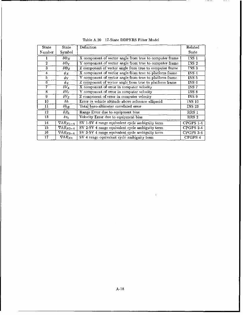
Table A.20 17-State DDPNRS Filter Model
State State Definition RelatedNumber Symbol State
1 6ex X component of vector angle from true to computer frame INS 12 61y Y component of vector angle from true to computer frame INS 23 6Ez Z component of vector angle from true to computer frame INS 34 Ox X component of vector angle from true to platform frame INS 45 Oy Y component of vector angle from true to platform frame INS 56 Oz Z component of vector angle from true to platform frame INS 67 6 Vx X component of error in computer velocity INS 78 6Vy Y component of error in computer velocity INS 89 6Vz Z component of error in computer velocity INS 910 6h Error in vehicle altitude above reference ellipsoid INS 1011 6hB Total baro-altimeter correlated error INS 23
12 6Rb Range Error due to equipment bias RRS 113 6 Vb Velocity Error due to equipment bias RRS 2
14 V6RN1_4 SV 1-SV 4 range equivalent cycle ambiguity term CPGPS 1-415 V6RN2-4 SV 2-SV 4 range equivalent cycle ambiguity term CPGPS 2-416 VbRN3 - 4 SV 3-SV 4 range equivalent cycle ambiguity term CPGPS 3-417 VbRN4 SV 4 range equivalent cycle ambiguity term CPGPS 4
A-18

Appendix B. Litton LN-93 INS Error State Model Dynamics and Noise Matrices
This appendix contains tabular listings of the elements of the LN-93 INS Error State Dynamics
matrix (F matrix) and the Process Noise matrix (Q matrix) developed by Litton. Both matrices
(F and Q) are 93 x 93 arrays which contain many zero elements, only the non-zero elements are
presented in this appendix. The elements presented in Tables B.1 through B.10 are taken directly
from (5).
Tables B.1 through B.8 list the sub-matrices of the F matrix. These sub-matrices are the
separate components of the F matrix presented in Equation (3.4) in Chapter III.
Tables B.9 and B.10 list the sub-matrices of the Q matrix. These sub-matrices are the
separate components of the Q matrix presented in Equation (3.4) in Chapter III.
B-1

Table B.1 Elements of Dynamics Submatrix F11
Element Term i1 Element T Termr
(1,3) -pY ]f (1,8) -CRY JJ(2,3) px I (2,7) CRX lJ(3,1) PY II (3,2) -Px(4,2) -Qz (4,3) _y
(4,5) wz (4,6) -wy
(4,8) -CRY
(5,1) QZ (5,3) -Qx(5,4) -wz (5,6) wx(5,7) CRX
(6,1) -QY i(6,2) Lx
(6,4) wY (6,5) -wx
(7,1) -2Vy Ly - 2VzQz (7,2) 2Vy Lx(7,3) -2VzQLx (7,5) -Az(7,6) AY (7,7) -VzCRX(7,8) 2 Q2z (7,9) -py - 2My(8,1) 2VxAy (8,2) -2VyAx - 2VxL2z
(8,3) 2Vz Ly (8,4) Az(8,6) -Ax (8,7) -2LQz(8,8) -VZ CRY (8,9) Px + 2Lx
(9,1) 2 VxLY z (9,2) 2Vygz(9,3) -2Vy zy - 2VxQx (9,4) -AY(9,5) Ax (9,7) py + 2My + VxCRx(9,8) -Px - 2LQx + VyCRy (9,10)(9,11) -k 2 (9,12) -1.0(9,13) k2 I I I
(10,9) 1.0 (10,11) k_(10,13) ki - 1.0
(11,10) 1.0 !1 (11,11) -1.0
(12,11) k 3 J[ (12,13) -- k3
(13,10)_ k4 (13,11) --k4
(13,13) k4 - 1
B-2

Table B.2 Elements of Dynamics Submatrix F 12
SElement ITerm Element J Term
(4)14) C1_t (4,15) C12t
(4)16) C13t (4,24) Clit(4,25) C1 2t (4,26) c13t
(5,14) C 21t (5,15) C 2 2t
(5,`_16) C23t (5,24) C21t(5,25) C 22t (5,26) C23t
(6,14) C 31t (6,15) C 3 2t
(6,16) C 3 3t (6,24) C 3 1t
(6,25) C32t (6,26) c33t
(7,17) Clit (7,18) C 12 t
(7,19) C13t (7,20) 1.0(7,27) Cllt (7,28) C 12 t
(7,29) C 13t
(8,17) C 21t (8,18) C 2 2 t
(8,19) C2 3t (8,21) 1.0
(8,27) c 2 1t (8,28) C22t(8,29) CI3t
(9,17) C 3 1t (9,18) C 3 2 t(9,19) C33t (9,22) 1.0(9,23) k2 (9,27) C 3 1t
(9,28) 632t (9,29) 633t
I (10,23) ] ki III II (12,23) -k 3 II I I
B-3

Table B.3 Elements of Dynamics Submatrix F1 3
[[Element Term]] Element Term
(4,30) C11 (4,31) C12(4,32) C 13 (4,33) Ciiwx
(4,34) C1 2wY (4,35) C13wz(4,36) Cilwz (4,37) C12wz
(4,38) C 1 awy (4,39) C11wy(4,40) C12wx (4,41) C13wx
(4,42) CTJw7 (4,43) C 1 2wL,
(4,44) C 1 3w2z (4,45) .5CllwxI(4,46) .5C121wyI (4,47) .5C13jwzI
(5,30) C 21 (5,31) C 22
(5,32) C 23 (5,33) C21WX
(5,34) C 22wy (5,35) C 23wz(5,36) C 21wz (5,37) C 22wz
(5,38) C 23wY (5,39) C 21wy
(5,40) C22Wx (5,41) C23WX
(5,42) C2 ,wx (5,43) c 22wy,(5,44) C 2 3 wz (5,45) .5C211wx1
(5,46) .5C 22Iwy1 (5,47) .5C231wzI
(6,30) C 31 (6,31) C 32
(6,32) C 33 (6,33) C 3 lwx
(6,34) C3 2wy (6,35) C33wz
(6,36) C 31wz (6,37) C 32wz
(6,38) C33LOy (6,39) C 3 1 Ly
(6,40) C32Wx (6,41) Ca33Lx
(6,42) C3 ,wx (6,43) C32 w'(6,44) Ca33w-- (6,45) .WC31 wxI
(6,46) .5C 32Iwy1 (6,47) .5C33IwzI
B-4

Table B.4 Elements of Dynamics Submatrix F 14
Element Term]] Element Term
(7,48) C11 (7,49) C 12
(7,50) C 13 (7,51) CllAT7(7,52) C 12AB (7,53) C 13A '(7,54) CI Ax1 (7,55) C127A6 .
(7,56) C13 1A"A (7,57) C11ABA
(7,58) C12ABA (7,59) C 13 AgA(7,60) C1 1A Au (7,61) Cji Au(7,62) C1"A"AB (7,63) .u uY-1 Y-X C12AyABz
(7,66) CliA•u (7,67) C12A•x(7,68) C 13 AB (7,69) -C13A
(8,48) C 21 (8,49) C 22
(8,50) C 23 (8,51) C-2A-I(8,52) C 22 AB (8,53) 623ABZ(8,54) C21JA 1 (8,55) C221A-I(8,56) -;C231Az (8,57) C2,ABx(8,58) C22AyB' (8,59) C 23 A B
(8,60) C21 AB A (8,61) C2 IAxAZ(8,62) C 22 AIIA (8,63) C 22 AByA(8,64) C 2 3A' A (8,65) "C28Ax5) C23 Y"•z
(8,66) C 2 1 A- (8,67) C22Aj(8,68) C 23AY (8,69) 7C23A(9,48) C 31 (9,49) C 32(9,50) C 33 (9,51) C31ABX(9,52) C 3 2AB (9,53) 633AB'
(9,54) C31 IA 1 (9,55) C3 2 JIA'I
(9,56) C33JAB J (9,57) C 3 1AB"
(9,58) C32A - "• (9,59) C3 A•
(9,60) C3 1AA f (9,61) -C3 - 'C1x AY C3Ax z
(9,62) C32Ay-A (9,63) C 3 2AAB(9,64) C 3 3 A (9,65) IC33A(xA5) C33AByAz
(9,66) C3 1A4. (9,67) C 3 2AU(9,68) C 33AI , (9,69) C 3 3A•
B-5

Table B.5 Elements of Dynamics Submatrix F 15
[[Element [Term [[Element I Term ]]
(4,73) [1, (4,74) C12
(4,75) C (4
(5,73) C21 (7,71)(5,75) C23 c_ _
(6,73) C3[ (8,71)(6,75) C33C3
(7,70) C1 (7,71) C ___12
(7,72) C13 1(8,70) C2, =8,71) L2(8,72) C23C2
(97) C31 (9,71) C32
(9,72) 033
Table B.6 Elements of Dynamics Submatrix F 16
Element Term Element Term
(4,76) CllA7 WibZ (4,77) CjlA7 wibY(4,78) Cl1A'WibX (4,79) 611A'Liby
(4,80) CllA'WibZ (4,81) C,1A~ wibx(4,82) C12A'WZibX (4,83) C12A'zwibZ(4,84) C12A'wiby (4,85) C12A'XwibZ(4,86) C12A'wibX (4,87) 612AI
(4,88) C13AAwby (4,89) C13AXWibX
(4,90) C13A'wibz (4,91) C13AI7iibX
(4,92) C13Aywiby (4,93) 1C13AuWibZ
(5,76) C21A'wibZ (5,77) CA1A wibY(5,78) C2'IA i'bx (5,79) C2lA y
(5,80) C2,AWibZ (5,81) C21AWbx
(5,82) C22A'wibx (5,83) C22A7 wibz(5,84) C22A'wibY (5,85) C22AXWibZ
(5,86) C22A'WibX (5,87) C22A WibY
(5,88) C23ABwiby (5,89) C23A':Tbx
(5,90) 623A~wibz (5,91) C23AyWibX(5,92) C23AAwiby (5,93) - 3 C23AwbZ
(6,76) C31AWibZ (6,77) C3,AiWibY
(6,78) C31A'wibx (6,79) C31A'LibY(6,80) C31AZ'Libz (6,81) C31A'Wibx
(6,82) C32A~wibx (6,83) C32AuLibz(6,84) 632AwzibY (6,85) C32A'WibZ(6,86) C32AywibX (6,87) C32A 3 by
(6,88) C33A'WibY (6,89) C33Aw ibX
(6,90) C33A'wibz (6,91) C33A'Wibx
(6,92) 633Aa wiby (6,93) U37Bw72
B-6

Table B.7 Elements of Dynamics Submatrix F 22
Element j Term Element ] Term
I (14,14) -fl_., [(15,15) -fbo
i (16,16)I-3o (17,17) -fv0i (18,18) I(19,19) I-i vzo I
] (20,20)i-Z3. ]f(21,21) -•LiJ (22,22) -)3aI (23,23) -2 o i
Table B.8 Elements of Dynamics Submatrix F55
i Element J Term Element TermlI (70,70) -• I (71,71)l-fiI
0(72,72) -/V~~(73,73) ~ J0 (74,74) -/b, JI (75,75) I--•k'A I
B-7

Table B.9 Elements of Process Noise Submatrix Q11
ft Element Term Element J Term
t (4,4) ] w,,, 55) I 'b
fI (6,6) ] •,27I (7,7) JY 71Ift (8,8) w,27 I (9,9ý)II,•
Table B.10 Elements of Process Noise Submatrix Q22
Element Term Element Term
(14,14) 2[lb,2lI (15,15) [•b cw, ]I(16,16) 2flb~o2 II (17,17) 2[0v W i
ft (8,1) [2!3vw~, II(19,19) 7~ ]ft (20,20) 2 6g~w6•,g II (21,21) /1 -6 g ]6 I
II (22,22) 2fbg~w6. II (23,23) [ZocW6 ho II
B-8

Appendix C. PNRS and DDPNRS Noise Matrcies (Q(t) and R(t)) Values
This appendix contains tabular listings of the truth and filter models dynamics driving and
measurement noise values. The tables with the dynamic driving noise values contain only the states
in which dynamics driving noise was added to other than the random processes from the models
themselves. Theses values are the scaling factors which come from (5,9,20,23,26,28,29) and from
the tuning conducted by this author.
C-1

Table C.1 PNRS Truth and Reduced Order Filter Model Tuning Values of Q(t) Matrix withVelocity Aiding
Truth State Truth Model Filter State Filter Model UnitsNumber Noise Value Number Noise Value 11 11
1 0.0 1 0.5 x 10⁻¹³ (arc-sec)2/sec2 0.0 2 0.5 x 10⁻¹' (arc-sec)1/sec3 0.0 3 5 x 10-14 (arc-sec)2/sec
4 190.4 x 10⁻¹⁵ 4 9.52 x 10⁻¹² (arc-sec)2/sec5 190.4 x 10⁻¹⁵ 5 9.52 x 10⁻¹² (arc-se)2/sec6 190.4 x 10⁻¹⁶ 6 95.2 x 10"1 (arc-sec)2 /sec7 102.9 x 10⁻⁹ 7 1.5435 x 10⁻³ ft 2 /sec3
8 102.9 x 10⁻⁹ 8 1.5435 x 10⁻³ ft 2 /sec3
9 102.9 x 10⁻⁹ 9 15.435 x 10⁻³ ft2/sec3
10 0.0 10 50.0 ft 2/sec11 33.34 11 1667.0 ft 2/sec12 0.0 12 5.0 ft 2/sec
13 0.0 13 1.0 x 10⁻¹⁰ ft 2/sec3
14 0.0 14 1.0 ft 2 Isec15 0.0 15 1.0 x 10⁻⁹ ft 2 /sec 3
16 0.0 not modeled ft 2 /sec17 0.0 not modeled ftT Isec18 (time-varying)notel not modeled ft 2 /sec 5
19 2.7451 x 10⁻¹¹ not modeled Pg 2 Isec20 2.7451 x 10⁻¹¹ not modeled pg 2 /sec21 2.7451 x 10" not modeled pg 2/sec22 1.9548 not modeled Pg2 /sec23 1.9548 not modeled pg' /sec24 1.9548 not modeled pg2/sec47 6.667 x 10⁻¹s not modeled ft2/sec51 6.667 x 10⁻¹³ not modeled ft 2/sec55 6.667 x 10⁻¹³ not modeled ft 2 /sec59 6.667 x 10-'3 not modeled ft 2/sec63 6.667 x 10⁻¹³ not modeled ft 2 /sec
67 6.667 x 10⁻¹³ not modeled ft 2 /sec68 0.0 16 2.0 ft 2 /sec69 0.0 17 2.0 ft 2 /sec70 0.0 18 2.0 ft 2 /sec71 0.0 19 2.0 ft 2 /sec
C-2

Table C.2 PNRS Truth and Reduced Order Filter Model Tuning Values of Q(t) Matrix withoutVelocity Aiding
Truth State Truth Model Filter State Filter Model UnitsNumber Noise Value Number Noise Value
1 0.0 1 0.5 X 10⁻¹³ (arc-sec)2 /sec2 0.0 2 0.5 x 10⁻¹³ (arc-sec)'/sec3 0.0 3 1 X 10-13 (arc-sec)2 /sec4 190.4 x 10⁻¹⁵ 4 9.52 x 10⁻¹² (arc-sec)2 /sec5 190.4 x 10⁻¹⁵ 5 9.52 X 10⁻¹² (arc-sec)2 /sec
6 190.4 x 10-:5 6 285.6 x 10⁻¹"' (arc-sec)21/sec7 102.9 x 10⁻⁹ 7 1.029 x 10⁻³ ft 2 /sec3
8 102.9 x 10⁻⁹ 8 1.029 x 10⁻³ ft 2 /sec3
9 102.9 x 10⁻⁹ 9 10.29 ft 2/sec 3
10 0.0 10 30.0 ft 2 /sec11 33.34 11 833.5 ft 2/sec12 0.0 12 5.0 ft 2 /sec13 0.0 13 1.0 x 10⁻¹° ft 2/sec 3
14 0.0 14 1.0 ft 2 /sec15 0.0 15 1.0 x 10⁻⁹ ft 2 /sec3
16 0.0 not modeled ft 2 /sec17 0.0 not modeled ft 2 /sec18 (time-varying)n"tel not modeled ft 2 /sec 5
19 2.7451 x 10⁻¹¹ not modeled pg 2 /sec20 2.7451 x 10⁻¹¹ not modeled P9g2/sec21 2.7451 x 10" not modeled pg2 /sec22 1.9548 not modeled pg 2 /sec23 1.9548 not modeled Pg2 /sec24 1.9548 not modeled pg 2 /sec47 6.667 x 10-'3 not modeled ft'P/sec51 6.667 x 10⁻¹³ not modeled ft 2 /sec55 6.667 x 10¹³ not modeled ft 2/sec
59 6.667 x 10⁻¹³ not modeled ft 2/sec63 6.667 x 10⁻¹³ not modeled ft 2 /sec67 6.667 x 10⁻¹³ not modeled ft 2 /sec68 0.0 16 10.0 ft 2 Isec69 0.0 17 8.0 ft 2 Isec70 0.0 18 2.0 ft 2 Isec71 0.0 19 2.0 ft 2/sec
C-3

Table C.3 DDPNRS Truth and Filter Model Tuning Values of Q(t) Matrix
Truth State Truth Model Filter State Filter MVdel UnitsNumber Noise Value Number NFie dlu U
1 0.0 1 0.5 x 10-l1 (arc-sec)2 /sec2 0.0 2 0.75 x 10⁻¹⁴ (arc-sec)2 /sec3 0.0 3 5 x 10-14 (arc-sec)2 /sec
4 190.4 x 10-'5 4 9.52 x 10¹² (arc-sec)2 /sec5 190.4 x 10⁻¹⁵ 5 9.52 x 10⁻¹² (arc-sec)2 /sec
6 190.4 x 10⁻¹⁵ 6 142.8 x 10⁻¹² (arc-sec) /sec7 102.9 x 10⁻⁹ 7 514.5 x 10⁻⁶ ft1/sec38 102.9 x 10⁻⁹ 8 514.5 x 10⁻⁶ ft 2 /seC3
9 102.9 x 10⁻⁹ 9 6.174 ft 2/sec3
10 0.0 10 30.0 ft 2/sec
11 33.34 11 500.1 ft 2/sec12 0.0 12 5.0 ft 2/sec13 0.0 13 1.0 x 10⁻¹⁰ ft 2 /seC3
14 0.0 not modeled ft 2 /sec15 0.0 not modeled ft 2 /sec16 (time-varying)n"tel not modeled ft 2 /sec 5
17 2.7451 x 10- " not modeled pg2 /sec18 2.7451 x 10'-1 not modeled pg2 /sec19 2.7451 x 10⁻¹¹ not modeled pg2 /sec20 1.9548 not modeled pgg /sec21 1.9548 not modeled Pg2 /sec22 1.9548 not modeled Pg'2 /sec45 6.667 x 10⁻¹³ not modeled ft2isec49 6.667 x 10⁻¹³ not modeled ft 2 /sec53 6.667 x 10⁻¹³ not modeled ft 2 /8sec57 6.667 x 10⁻¹³ not modeled ft 2 /sec61 6.667 x 10⁻¹³ not modeled ft 2 /sec65 6.667 x 10⁻¹³ not modeled ft2/sec66 0.0 16 10.0 ft 2/sec67 0.0 17 4.0 ft 2 /sec68 0.0 18 2.0 ft 2/sec69 0.0 19 1.0 ft2 /sec
C-4

Table C.4 Measurement Noise Covariance Values of R(ti) Matrix for PNRS Filter
Measurment 1 Truth Model Value Filter Model Value Units
RRS Range 4.0 6.0 ft 2
RRS Velocity 0.09 0.12 ft 2 /sec 2
DGPS 9.0 30.0 ft2CPGPS 2.641 x 10- 3.0 10-4 ft 2
Baro-altimeter 2500 2500 ft 2
Table C.5 Measurement Noise Covariance Values of R(ti) Matrix for DDPNRS Filter
Measurment 11 Truth Model Value if Filter Model Value Units
RRS Range 4.0 6.0 ft 2
RRS Velocity 0.09 0.12 ft 2/sec2
DGPS 9.0 30.0 ft2
CPGPS 2.641 x 10⁻⁴no•e• 3.0 x 1 0 - 4 note2 ft 2
Baro-altimeter 2500 2500 ft 2
Notes:
1. Time varying from 0.0 to 26.9667
2. Values presented are for Satellite #4 only. The values used in the differenced pairs is twice
that of the presented value in Table C.5.
C-5

Appendix D. 71-States PNRS Filter without Velocity Aiding Results
This appendix contains the plots using Hansen's 71-State PNRS Filter without the Perfect
Doppler Velocity Aiding measurements. The plots are ordered as in (9) for direct comparison
between these plots and those of (9).
A legend for the presented figures is given below.
Table D.1 Legend for Filter Tuning Plots
Symbol Definition
- Solid Line Mean Error... Dotted Line Mean Error ± True Sigma
- - Dashed Line + Filter Predicted Sigma
D-1

1 0
8 ..
1018 00
6I I!I f;I
0 il
0 1000 2000 3000 4000 5000 6000 7000
Tie(sc
8 ~ ~ ~ Fgr D. 1- Logiud and Latitude- Error........ Plots---------
... .. ... .. ....D-2..

* .. .. 11
1 5 --- --- -- --- -- -
-5 -
-10
o 1000 2000 3000 4000 5000 6000 7000
80
6 0 - ---------. .... ........ .... ......
40
-620
D D3

X10,
-1. ... .. .. ..*- -- - -- --
0 1ý5. 6
o- - ----r- --- -- - - -
0 1000 2000 3000 4000 5000 6000 7000
x 1o3
I I
E II
CD.

WON 1V I0 . Il ]II
>0.5 w
0 00 20 00 400 50 00 70
T5 5
0 1000 2000 3000 4000 5000 6000 7000
II it-oil
01 iNI:
LI I j 'liii *....i. ...U ±'iIJ i d..... .
0 1000 2000 3000 4000 5000 6000 7000
Tie(sc
1iur DA4lt*4*4**l~ North Wet *n etclVlct ro lt
0-

. 42
' C 0.015W 40'1
"" . .. . . .C 2~o
-0.015
0.0
x -0 .005 .... ........
0 1000 2000 3000 4000 5000 6000 7000
E
0 1000 2000 3000 4000 5000 6000 7000Time (sec)
Figure D.5 RRS Range Bias, Range Velocity, and Atmospheric Propagation Delay Error Plots
D-6

10,
....... ............2 5 .".:.. .. .... ............ .-.-. ...-.. ....... .-
LUJ0
' --- 0 .. .. . .. . . . . . .. . . . . . . .. . . . . . .. . . . . . . . . . . . . . . . . . . . . . . . . . . . . . . . . . .
(I50
o1 100 200 30 00 50 00 700 1000 2000 3000 4000 5000 6000 7000
10 1
Tie(s•
S5 - . . . • . ...: . . .. . .. . . . .. ..... . . .. . . .. . ... . . .. . . . .. . .. . .. ... . . I .. .. ..... ..I ....
LU ..... ." -.-'...' .i• .•- .. . .• .: . .• . . -. .... .. ..- ..-.... .... !. . ....... ..... i ........ ........ ... .. .... ...... ..
• -- --- - .. ... . . . .... . ...- . . ..:.0'a..-." ....-..- :. ... . . .••.- .. .. _ . ....... ... . ..._..- ..... ....
rn -5 ---- --- ------- :. . . . . .. ... . . . .. . .. . . .. . .. . . .. . .. .... . . .. . . .. . .. . . .. . . .. . .. . . ..-I. . . .. . .. . .. . . ...
cc
-10D0 1000 2000 3000 4000 5000 6000 7000
10
-,,, - -. - 7- -C ".. . .. . . . . :.. . . . . . . . .:. . .. . ... .. . ... : .. . .. . .. . ... . ! . ... ............:• 0 ..... ... ...... .. . .. ...... .. . . . . - !
Z,,.. . .... ..... ....... . ........ . .. .. .
N -..• _ . . : L . - .- : .• -,•• ",:"': .. • ""-"• • - -- ".• --- "- - -- -- - - --
CO -5 .cccc
-100 1000 2000 3000 4000 5000 6000 7000
Time (sec)
Figure D.6 RRS X, Y, and Z Position Error Plots
D-7

4 - . .. - - - -- - - - I- - - - - . . . . . .. . . . . . . . . . .. ... . .. . .
11111 i0 611 j ill* I 1I~ ll. II I; ]ill~i, I 1 .1 1 1
-.25
1~ 0.2,11,111 1 -JIVi.
0
.2. .... .. ... ......0.. ....0 5- -- -- --- . .. .
~ 0.1-
-0.2 5 - 1- - . .. . ....
0D-

10 I I I
8
, ', , -6
6 . . . .. . . .. . ...-- -. .. . . .. . . . .. . .i. . . .. . . .. . . .. .!. . . . .. . . . . .. . . -----.. .. . .. . . .. . .! . . .. . .. . . .. . ... . . . .. . . . .i
>-8i
0 . -64 - . . . . . . . .. .. .. . ... ... . -- -- -- --. .. ... .......... . . . . . . ... ..... ... .... .... ...... ....... ... ... .. ... ...
"8
-0
S-2
0 1000 2000 3000 4000 5000 6000 7000
10,,, ,
8 . . . .. . . .. . . . . :. . . . . ... : . . . . . . . i... .. . . .. . .. .... . . . . . . . .!.. . .. . . .. . .. . .-- - --- --- - --. . . . .. . . ....-- -- --- -
"0 4 ........ .. ',.............. ........ ........ i....... ........ ....... i-
S2
" 0E
CL -64 .. . . .. . . . .. . ....... . . .. . .. . . . ....... . . .. . . .. . ..--.. . . . .. . .. . ..--.. .. . .. . .. . .. . ---.. . . .. . ... ... i.... .. . . .. . .. ..... .
-8 . . . . .. . . .. . ..- -. . . .. . . . . . ... . .. . . .. . . .. . ... --. .. . . . . . . .. .. . . .. . .. . ... .. ----------------- --.. . . . . ..- --- -
-10 ,0 1000 2000 3000 4000 5000 6000 7000
Time (sec)
Figure D.8 GPS Satellites 1 and 2 Phase Ambiguity Error Plots
D-9

101r1 11
8 - - -- - - -- - - - - - -I . . .. .. . . ... . . . . . . . . . . . . . . . . . .. . . . . . . ..
4C.,
2 -
-8 .. ..
CL4
I' - 6 - -- - - -I - - - - - I- - - . . . . . . - - - - - - - - - - -
0 1000 2000 3000 4000 5000 6000 7000
D-01

Appendix E. Reduced Order PNRS Filter Results with Velocity Aiding
This appendix contains the results from the two-hour simulation run of the Reduced Order
PNRS filter. The results presented still contain the perfect Doppler velocity aiding measurements.
These results are used for direct comparison with the same filter run without the perfect Doppler
velocity aiding measurements of Appendix F. The plots are in the same order as Appendix D, also
for direct comparison.
A legend for the presented figures is given below.
Table E.1 Legend for Filter Tuning Plots
Symbol DefinitionSolid Line Mean Error
... Dotted Line Mean Error ± True Sigma
- - Dashed Line + Filter Predicted Sigma
E-1

15
0 ..Fi.. . . .. .. ... . i.. .. . ... ... ... . .. . .. .... .. .. ... ... .. . ]. • •... ... . .. ... ... .. .... . .. ... . .. .. . .. ... ... ...... ..
S5 .. : -.. . . . . . . . : . . . . . . . ... :.: ..- •.:-• " . .' .' . . . . . . . . . . . . . . . . ... . . . . .. - . . . . . I. . . . . . . . . . . . . .. ' . . . . . . .:. _
ILl
- .. .. ... . .. .... .. ..... . . . ...... . . .- ---
-1 0 - - - - --. ... . .. . . . .. ... . ... . . . . .. . .. .:. . . . .... . .i . . . . .. . .. . . .... .. . .. . . .. .. . . .... .. . .. . . .. . . .... . . . . .
-150 1000 2000 3000 4000 5000 6000 7000
15,, ,,,,
1 0 . . . . . .. . . .. ... ---------. . . . ... .. . . .. . .. . . .. . .. . .. . . .. . .. .i. .. . . .. . .. . .. . I -- -------------I . . . .. . .. . . .. . .! --
(D 0 - - - . . . . . .. . .. . . . -- -- -- -- -
S5 ............. : ="". ........................ .............. @ " :'"-'"•,"o" "''... ..... . ...
u•0
-j -5
- 1 0 - -------------. . ... . .• '- - -' : : .... . .... ... .. -- - - - - --.. . . . . -- ---. . - - - - - - - - - -. . . . . . . .... . . . . . . . . . . .
-150 1000 2000 3000 4000 5000 6000 7000
Time (sec)
Figure E.1 Longitude and Latitude Error Plots
E-2

20
-5
-200 1000 2000 30 00 40 00 50 00 60 00 70 100
80
60
'-20
0
6-60
-80
800 1000 2000 30 100 4000 50 100 60 100 70 100Time (sec)
Figure E.2 Altitude and Barometric Altimeter Error Plots
E-3

X10-
wD=7
S)
0z
0 1000 2000 3000 4000 5000 6000 7000
1
wM7--- - - - '- - - -7
0 1000 2000 3000 4000 5000 6000 7000
LU 0

0.2
0.
w>~ 0
0z0. -
0 1000 2000 3000 4000 5000 6000 7000
0. I I71
wi
0)
0 1000 2000 3000 4000 5000 6000 7000
. .. . .. ..* .... . . . .
wo
75-0.1
0 1000 2000 3000 4000 5000 6000 7000Time (sec)
Figure E.4 North, West, and Vertical Velocity Error Plots
E-5

10II
6 -2 --- --
4u
CL-8
0 1000 2000 3000 4000 5000 6000 7000
0.015 II
-0.005.....---............... .............. .............. ----2
I.- .......-- -- - --...... ------ 1'ý.......
*i-0.015
0 1000 2000 3000 4000 5000 6000 7000
Figure E.5 RRS Range Bias and Range Velocity Error Plots
E-6

4
0
0
0.
0.5 . . . . . . ........... ............. ........... ---------------..................
4 o.i....................... ......
S0.05-
0 . 5 t -----o-. ........ ...... .... ... ....... ..............
0.1--- - - ----------------------------------------
0
-0.05 ---
-0.15 .. . .. .. .. . ... ... .. ... . .. . .I. . ...................... . ... .... .. .....
-0.20 1000 2000 3000 4000 5000 6000 7000
Time (sec)
Figure E.6 GPS Clock Bias and Drift Error Plots
E-7

10
6 ............
4-8- -- .. .. . ..
wS2
I I
0 1000 2000 3000 4000 5000 6000 7000
Tie0sc
Figure.. ........ 7.. GPS Satllies..an.2.hae.AbigityErrr.Pot
.. ... .... ... .. .... . .. .. .....

10 I
.. . . . ...4. .. . . . .. . . .. . . . .
-2 ....
-8
0 1000 2000 3000 4000 5000 6000 7000
10
6 ........... -------------------- ................................................. .. ..
--- -- ----------......... ............. . . . . . .
-~ - - --4
I Ij
0........ 100 200 300 4000- 5000 6000 -- 7000Tie(sc
Fiur E---- 8 GPS- Satllte 3-n- hseAbgiy rolt
c/E-2

Appendix F. Reduced Order PNRS Filter Results without Velocity Aiding
This appendix contains the results from the two-hour simulation run of the Reduced Order
PNRS filter. The results presented do not contain the perfect Doppler velocity aiding measurements.
These results are used for direct comparison with the same filter with the perfect Doppler velocity
aiding measurements of Appendix E. The plots are in the same order as Appendix D for direct
comparison.
A legend for the presented figures is given below.
Table F.1 Legend for Filter Tuning Plots
Symbol Definition
Solid Line Mean Error• Dotted Line Mean Error = True Sigma
- - Dashed Line - Filter Predicted Sigma
F-1

15
SL -
5-
-I 0 . . . . . . . . .. . . . ... . .. . .. . . . .. . . .. : .. . . .. . . .. . .. . -------- . . . .. . . . . . : . . . . . . . . . .
0
C
-J-5
-10- 5 i i I
0 1000 2000 3000 4000 5000 6000 7000
15
1 0 .- - .-- -- .-- - .--.------.-.---. . . .... .... . . . ... ... ... .. I ..............
S5 :: . . . . . . . . . . .. . . :" . ....:' '.... .. ,. . . . .. .. . . . . . . . . . . . . . . . . .. . . .. . . . .. ." '• . . ." -", ..- '-. _. .-. . - ,. '- .: - .<j
0
"-J -5- . ... . . . .. . . .. ... ..... . .. -- ------ - -. •• • • z-• "S . ........~~~~~:" .........-:•, • . .- •.--.•-... -
-10
-150 1000 2000 3000 4000 5000 6000 7000
Time (sec)
Figure F.1 Longitude and Latitude Error Plots
F-2

20
15~ ~~~~~~~~~ ~~~~ .. . . ... . .. . . . . . . .. . . . . . . . . . . .... .......... -: ......... . . . .:
-1 5 ---- ---- ------ ----------. .. .-- ---------------. . .. . . .. . ... . ... : .. . .. . . ... . .i . . . . . . . . . . . . . . .! -
-10 ---..-. -.-. --.... ............ --............................ .. .................................. .....
~J
-5
80
60 o
61 0 ... • _ .... . ... ... ... ... ... .. .... _. . . . . . ...-- -- --.... . .... .. .. . . ...... .. . _!
4 0 . .... . . . .. . . .. . . :..
40
. o.
-0-20
' , - . .. .. . :. - , •
-6 0 . . .. . . . .. . . .. .i.. . . . .. . . .. . . .... ... . .. . . . .." . . . .. . . .... .i .. . .. . .. . . .. ... • . .. . .. . .. . .. .. . . . .
0 1000 2000 3000 4000 5000 6000 7000
Time (sec)
Figure F.2 Altitude and Barometric Altimeter Error Plots
F-3

CD-0 - - - -
zRCD
0S00O0 00 400 50 00 70
... ... ...
.. ........
0 1000 2000 3000 4000 5000 6000 7000
X00-
CD
I-
0 1000 2000 3000 4000 5000 6000 7000
Tim (1ec)
FiueF1Nrh etadAiuhTl ro lt
CD4

1. IA --- --
...... .... ........
> -0 5 -- --- -- --
zV
0 1000 2000 3000 4000 5000 6000 7000
0 ..... . -....
:-f -. -- - Mt - -- -
> -0.5III
0 1000 2000 3000 4000 5000 6000 7000
o0
- - - - - - - - - --)5~~ ~~~ ~ ~ ~ ~ -I-- -- - - - - - - - - - - - -- - - - - - - -- - - - . . . . . .I .. . . .. . .
0 1000 2000 3000 4000 5000 6000 7000Time (sec)
Figure FA4 North, West, and Vertical Velocity Error Plots
F-5

10I
c 2
cis
-80
0 1000 2000 3000 4000 5000 6000 7000
0.015 I
0.01
0.005.....------............... --------
w
CL
x-0.01 - - - -
-0.015 II
0 1000 2000 3000 4000 5000 6000 7000
Figure F.5 RRS Range Bias and Range Velocity Error Plots
F-6

6
0 ji
0
-60 1000 2000 3000 4000 5000 6000 7000
0.2k-------------.............-------- .-.-- .--- .--- ....... . .........
0 .. ... ... . . .-.--.-.-.---.----.-- -- -
0 0..................... ................ .........................
0
-) 0.15........-.------..-----.---.--.-----------
-0.2 I
0 1000 2000 3000 4000 5000 6000 7000Time (sec)
Figure F.6 GPS Clock Bias and Drift Error Plots
F-7

10
U6U2 - - -- -- -.. . . .. .
2w
-8 . .... .. ... ... ---- ----
-2 - - -- -- . . . . . . . . . . . . . . . .
0 1000 2000 3000 4000 5000 6000 7000
: 2
2' -2 - -- --- ---
-: --
4 _ _ _ _ -- - -- - -- --__ _ _ _ _ _ _ _
0l 100 20700 400 50;00 70Tie(sc
Figure~~~~~~~ F. -P Saelie 1 an 2 Phs Amiut Ero Plt
-6 .. .. . .. . ... .. ... .. ... .. .. ..-- --- -- --- .. . .. .. . ...F -.. .. .

10
-- - - - -- - - - - -- - - - -8O -6 - - - - - . . . . . . .. .. . . . . - - - - - . . . . . .
1. . . .. . . -- - - - --I. . . . . . .I -- - - - - - --
8j
-4 ~ .....
Scr
-10
0 1000 2000 3000 4000 5000 6000 7000
Tie(sc
Fi ur F--- ------ -- - - .. ...... GPS...... Satelites..and..Pha e.Am b guity Error Plot
6 ..... ... ..... . .... ... .. ... .... .. ... .... .. .. .--- --- -- --F- --- -- -

Appendix G. The Double Difference PNRS Filter Results
This appendix contains the results from the two-hour simulation run of the Double Difference
PNRS filter. The plots are in the same order as Appendix D minus the GPS clock error plots which
are not modeled in this filter. The ordering of this appendix is for direct comparison to previous
results.
A legend for the presented figures is given below.
Table G.1 Legend for Filter Tuning Plots
Symbol Definition
Solid Line Mean Error... Dotted Line Mean Error ± True Sigma
- - Dashed Line ± Filter Predicted Sigma
G-1

10
0 ~ ~ - ---.-- --- -. ... ..-..-. .-. .-
.0 .w 5 ...w,- ..... - ..... .. .. ... . .. ....
1J5
1 0 - - -- -- - - . . . .. . .- - - - -
1 5 I1 I1,111 1 1
10
-10
0 1000 2000 3000 4000 5000 6000 7000Time (sec)
Figure G.1 Longitude and Latitude Error Plots
0-2

20
1 5 .. . . . .,. : - - - - - --.-- -
1 0 . . . . . . . .. . . ... . .. . . .. . . .. . . ...: . . .. . . . .. . .. . . . . . .. . . .. . .. . . . .. . . .. . . .. . .. . .. . . .. . .. . . .. .I. . .. . .. . . .. . . ..
1510
-10
S-5
-1 0 - - -- -- - -- -- -- --.. . .... ... . ... . . . .. . .. . . . .. .i . . . . . .. . . . . .. . .. . .. . .... . . .. . .. . .. . .. I . . .. . . .. . . .. . ..... . . . . . . .
-1 5 - - - --- -.. .. . .. ... . . . . . . ..- -.. .. . .. . .. . . .... • .. . .. . . .. . . ... -------. . . . . .. .. . . . .. . . .. . . .. ... .
-20i
0 1000 2000 3000 4000 5000 6000 7000
60
40 x
-40
4 0 : • :•-::..............
S20
-600 1000 2000 3000 4000 5000 6000 7000
Time (sec)
Figure G.2 Altitude and Barometric Altimeter Error Plots
G-3

X1-4
2 ... ......
0z
0 1000 2000 3000 4000 5000 6000 7000
X10-
SCD
.. ..... . .. . . . . . .
0 1000 2000 3000 4000 5000 6000 7000
X00,
I-
cm05(D 0 5. . . . . . . . . . .I- --N. . . . . . . . .. . . . . . - - - - - - - - - - - - - --
... ... ..........
0----- 100- 200-300-00-500-600-00LU ~ ~ ~ ~ ~ ~ ~ Tm (sec). ... ..........
Figre 3 ort, Wst.nd.zimth.iltErrr.Pot
-- ------ ---- - . .4 .

0.-
z 0 .0 00 20 004-0 50 00 70
....w. ............ -- --------- ----------
-0.5 -- -- -
0.5...........................
CD
5 ~..........
8U1114 111 11 1110
0
(D
0 1000 2000 3000 4000 5000 6000 7000Time (sec)
Figure GA4 North, West, and Vertical Velocity Error Plots
G-5

10
8 -- --- ---... .. ..I ... .... .... ......... ...I. ... ....I
6 . .... ...- --- -. . .......... .... .... ..
01
-10
0 1000 2000 3000 4000 5000 6000 7000
0.02 I
0 .0 1 5 -- --- -- -- - - - - - - - - - - - - - -- - - - - - - -- - - - - - ---.- - - - - - - -
. . ..0. . . .. . .. . . . . . . . . . . . . . . . . . . . . . . . . . . . . . . . . . .
a) 0.01
0)
CL 0.010...
~-0.025
0 1000 2000 3000 4000 5000 6000 7000
Figure G.5 RRS Range Bias and Range Velocity Error Plots
G-6

10
8 2- - -- - -- -- . .. ... ..... .... ... .. - -- -- - -- -- -
................. -2---
- - - - - - - . . . . . . . . . .. . . . . . .
4~
UD
-8. .. . .
1 0 .. .. .. .. . . . . . . . . . . . . ..- - - -.I. . - - -
.. .. .. ...8. . ... . ...
w 2 - -----
cCL - - - --- -- -- -- -.. . .... . .. ..
0 1000 2000 3000 4000 5000 6000 7000
Tie(sc
G77

2 4 .- - -----I-
10 r
8- - - - --- ......... .......... ........... ...... -------
Sc"
-10
0 1000 2000 3000 4000 5000 6000 7000
Tie(sc
Figure.... G.7- GPS- Satellite 3 and4.Pas.AmigutyErrr.Pot
8 --- -- -- ---- ---- ----- 8- - - .. .. ..

Appendix H. Double Difference PNRS Small Cycle Slip on Satellite #1 Results
This appendix contains the results of the 1000 second simulation run of the Double Difference
PNRS filter with a small cycle slip on satellite #1. The plots are in the same order of Appendix G
for direct comparison.
A legend for the presented figures is given below.
Table H.1 Legend for Filter Tuning Plots
Symbol Definition
Solid Line Mean Error... Dotted Line Mean Error ± True Sigma
- - Dashed Line ± Filter Predicted Sigma
HI-1

15
00
0)h
.- 5
-10
0 100 200 300 400 500 600 700 800 900 1000
10
l o I. .. . . .- - - - - . . . . .. . . . . .. . . . . . . .. . . . .. . . . . . - - - - - - -
w -
~ ~1~ttib, nt <t~'4' ti\ 4~~Vi ~tN';Hf ii~ 'ltf II ~tHT tf,~ I4Lif rJ777IW 1
-152

15
5 ~ L .i .rggL .D r1 m .111 --~., - -- .. .......
10
w -
5D
.. .. . ..1 0. .. . .. .. . . .
-1 5 ----------... ... ..... ....
o<0 0 0 0 0 60 70 80 90 10
40 ~OOOGOOOOOOOOOQ
-203

x 1041 I I
------- ...... ......
• '1 0 .5 ..... .~. .• ::: . .. ... . :. -: ..-..'. ............... •....... ....... . .................. .. ......
2 0 - -- ---. ' ' . .: . . . . . . .. . .. .. . . . . . . .. . . . . . . . :. . . . . - . . . . . ,- . . . . ,._ .
w i: : ... . :.. . .. .. . .. ... . .. .. .. .. ... .. .. ... ..... .. ... .. ...... ... ... .. ... .. .. .. ..i.. ... .... ... ... .... ... .. .. .. ... ...-0 .5 . .. ..- - - - - -
0
1 0
CD 0 .5 1 ..... . .0, -o ......... :......... = -.... .. .. .- • . . . . . . .. ........ .......... i .......... : . . . . ....... -
O
-1 I .I I .......
0 100 200 300 400 500 600 700 800 900 1000
X 10-3
1.5 -•- 7 I I
® 1'
.. . .. ....
0
o .0 . .-- : --- -• . . .. . . . . . . .:... ..... ...... ... :... ..... :... .. ... -- ------..
0~~~.. . . . .. . ... .... :::: .. . - , • . .,.. .... : ........... ..... ....... . ......
• -' ..........-i .. ... .. .. .
w 0.5 ...... . .
07
a ) -1 . . . . . . . . . . . . . . . . . . . . . ... . .. . . . . . . . . . . . . . . . . . . . . . . . . . . . . .
-1.5 I I I I
0 100 200 300 400 500 600 700 800 900 1000
x 10_- 1
i® 0.5..................................
E
0 10O0 200 300 400 500 600 700 800 900 1000
Time (sec)
Figure H.3 North, West, and Azimuth Tilt Error Plots
11-4

-0.2 --- - .. ... ... .
0z .. . . . . . .. . .......
0 ........ ...........-- -- --- - - - -
0 VI ........
0 100 200 300 400 500 600 700 800 900 1000
0.55

8
-2
-4
-0.05........................................ ............
CO
a
(a-0.01. ... ... .. . . . . .. . . ..
0 100 200 300 400 500 600 700 800 900 1000
Time(1ec
Figure ..11.5 RRS. Rang Bia Range Velocity and Atmospheric PrpaatonDeayErorPlt
........H. .....6.. .

20
.15
5~ %WMMWAWNWMNMME
> -5
CO10~
0 100 200 300 400 500 600 700 800 900 1000
15
L..
cm..............................
C/,
0 100 200 300 400 500 600 700 800 900 1000Time (sec)
Figure H.6 GPS Satellites 1 and 2 Phase Ambiguity Error Plots
11-7

5 IIII II
E
CD
--i
0 100 200 300 400 500 600 700 800 900 1000
3 L - .........
CO..
0 10 200 300 400 00 60 70 80 900 100Time... (sec).. ..
Figure -- 11.7.. GP Satellite 3.nd4.hseAmiuiy.rorPlt
11-

15,
- -- - -7 7 . . - .7 .. . . . . . .
00
-5 ---- --------------------------------- ..... ------ --- -------------
0 100 200 300 400 500 600 700 800 900 1000
111-

15,
-1 0
-5..... ----------------------....------------......-------------------- -
Ch
0-6
-15
0 100 200 300 400 500 600 700 800 900 1000
1H 1

Appendix L Double Difference PNRS Satellite #1 Loss Results
This appendix contains the results of the 1000 second simulation run of the Double Difference
PNRS filter with a GPS satellite loss on satellite #1. The plots are in the same order of Appendix
G for direct comparison.
A legend for the presented figures is given below.
Table 1.1 Legend for Filter Tuning Plots
Symbol Definition-Solid Line Mean Error
... Dotted Line Mean Error ± True Sigma- - Dashed Line ± Filter Predicted Sigma
I-1

15II
10 ... .. ..
C
-10
0 100 200 300 400 500 600 700 800 900 1000
10,
L.0 - - . . . ..- . . . . .. . . . . . . . .
-10
o 10o 200 300 400 500 600 700 800 900 1000Time (sec)
Figure 1.1 Longitude and Latitude Error Plots
1-2

"15 r I I I I I I
15
10
5 ~ ~~~~ .......... ... .. ....... ............................
60o
I. ..
0
-1 5 . .. . . . ... . .... .. . . i ... . .. . .. i ... .. . .. i . . . .... . .? . . .. .. .. .. ., .. .. . .. ...-.. . .. .. . .. ,. .. . .. . .. . .. . . .. . ..-
-20
0 100 200 300 400 500 600 700 800 900 1000
60, , , ,
4 0 - -- - - - -- ...... ..... ---- ,--
20 °
S-40 RAM 0
-60 ,,,,,, i0 10O0 200 300 400 500 600 700 800 900 1000
Time (sec)
Figure 1.2 Altitude and Barometric Altimeter Error Plots
1-3

x 104
--0.5
I l . . . . .. : . ... . . . . .. .. .I ".. . . :.. . . ..... . .. . . .. ... ... .. .. . . . . . .. . .. . . . . . . .... . . . .. . .. . . . . .. . . .. . .. . .. . . .. . . ..
.. - . . ........ . -.. .... - :' - ..... . . .•.. - .= • _. _ - i , _ . .... i - - - . . _ - - . .: .L .. _ . .. • -.. -. -...
o0Z
0 100 200 300 400 500 600 700 800 900 1000
x 1041.5 I ! , . . .
S0 :: : : : : : : r,.'. . '.-. . -.-.. .... ......... . . . . . . . .. ... ,,. ....-. ...- -... . . .:. : . . . . .
" 0 '. . . . . ... .. .. . . .. . .
0.
1 - . . . . ... . . .. . .. . .. . .. .. . .. .. . .:. . .. .. . .. . ... . . .. .. . .i . .. . .. ... . . .. .. . . .. .. . .. .. .. . .. .i .. .. . .. . ..: .. .. . .. .
-1.50 100 200 300 400 500 600 700 800 900 1000
x 10.3_ 1 I' I I II
0 .5 ......
® 0 . . ... • • ...... .. . . .. .... . . . .. . •...... ... . .... ...... ' ....... ... - . ........ :. . .. .... ... , . .......0
0 - - --- .........0.5 .......... --- - . ........... : ..............................S. . . .... . .. .. . . .. .. . .. . . .. . .. ... . .... . . . .. . .. . .. ...
I~j 0-........................ - - - - - - - - -
"- . .. .. .. 7 - - -
E-I
0 100 200 300 400 500 600 700 800 900 1000Time (sec)
Figure 1.3 North, West, and Azimuth Tilt Error Plots
1-4

S 0 .2 - ---- --- • . . . . . . . .. .. . . . . .. . . .. . .. . ... . . . . .: . .. . . . . . . . . . . . . . . . . .... . . . . .. .. . . . .. .:. .. . . . .. : . . . . . ....
0 . ." .. "".........-'-""....... : " ..... ... -.. ,. ... .'...-.'-..-............ . ....... .. .. ' .. .. '
>,00 '
0 V - ', .. ....... "'". ......."'...................
V -0 .2 .- - -- - -- - - - - -- . . .. . .. . . .. ... . . . . . . . . .. . . . . .
Z -05I I I
0 100 200 300 400 500 600 700 800 900 1000
0.5 !
w .. .. .. .... ...
" •. . . . . . . . . .. .. . .... .
> • ..............
S-0.5,, ,,0 100 200 300 400 500 600 700 800 900 1000
4 -- -- -- .......... ... ..... .. - - - ..o ...: ' : .-. ... '....-...-.. .. .:. .. .::" .- ...-- - . . .-
"51
• ! -4 . . . . . . ..• . . . . . . . . . . . . . . : . . . . . . . : . . . . . . .:. . . . . . . .. .: . . . . . . . . . . . . . . . . . . . .. ,. . . . . . . . . .:. . . . . . . . . .
-6-

8
6 -- -. .. . . . . . . . .. . . . . - - - -
w
-2
-40 100 200 300 400 500 600 700 800 900 1000
0.015I I I I
0.005
w . 0 . . . . . .- - - - .. . . . . . . -- - - - - -
CO 0 ----------- .......... ................................................
j-0.005 .. ....... ... ...------.......... ...................... -- --..................
a Ix
-0.015
0 100 200 300 400 500 600 700 800 900 1000Time (sec)
Figure 1.5 RRS Range Bias, Range Velocity, and Atmospheric Propagation Delay Error Plots
1-6

40
30 - --- - . ..2
10I .. . . . . . . ./.................. - - - - . . . . . ..................
E~~~~. . .....5tM fIA ISIIMWMfI.. ... . .
~-0
-4 : ..... ... ....................-----..........
-5a.II> 20 100... 200.... 300.... 400...... 500 600 700 800 900 100
CO,
C/,
0 100 200 300 400 500 600 700 800 900 1000
157

-j3 OWN~si~~
I I
0 .. .. .100 -- -- 200 .. .. 300 .. .. 400 . .. .. .. ..500. .. 600. ... . .. .700-- -- 8000 1 0
-.4
w 0 0 0 0 0 60 70 80 9010
61
--- -- ... .. .. ... ... ..--- -- .. ..
.. . . . . . . . .
-- - - - -- - - -
2 31 ' ... ... .. ... . .. .
3 jI
0 100.. 200-300-400 -500 -600 700. 800.900.1000
......... Tim (sec)---- .... .... .
Fiue17GSStlieE n hs mirt ro lt
-3-

601
-0
.,L -20 --------- ........ -... -...-..........------------------...........------ ---- -
140
60)
0W;-
0 0 0 0 0 0 60 70 80 9010.Time...ec)
-1-9

15,
0~
CO,a......... ....0. ..... .... --- ..... ----- .....- ----
0 100 200 300 400 500 600 700 800 900 1000
1 05 ... .. . .. . -- - -- - -- - -- - -
10
a:
------ .............................. .......
- - - - - - - - -- ------- ------ --- -------- ----
-101

Appendix J. Double Difference PNRS Large Cycle Slip on Satellite #1 Results
This appendix contains the results of the 1000 second simulation run of the Double Difference
PNRS filter with a large cycle slip on satellite #1. The plots are in the same order of Appendix G
for direct comparison.
A legend for the presented figures is given below.
Table J.1 Legend for Filter Tuning Plots
Symbol Definition
-Solid Line Mean Error... Dotted Line Mean Error ± True Sigma
- - Dashed Line + Filter Predicted Sigma
J-1

II I I I I I III
0
-1 0 0 0 -----.. .. .. ------.. .... . .. . .. . .. .. ..... . . . . . . . . . . .. . . . . . . . . .... . .. .. . .. .... . . . . .. ... . .. ...- - - - .. .. ..
- -2 0 0 0 r ......... .......... .......... .......... -- -- --......... ...... ... .............. ........ . . . . .. .. . . . . . . .-200
wS-3 0 0 0 ----.... ........... ..................... ... . ..................................................... .....
0
-4 0 0 0 T . ........... . ............... ........ .................. ..... ................
-5 0 0 0 ..... ...... ..... .... ............
-6000- I I0 100 200 300 400 500 600 700 800 900 1000
500....
0
-1500
w
=- 10 0 0 .......... .......... .......... ......... I............. . .. . . . .. . . . . . . . . . . . . . . . . . . . . .Nq
--------.. . . . . . . . . . . . . . . .. . . . . . . . . . . . . .... . .. .. .. .. .. . . .... .... .. . ....- ------ ------------. .. .. .. ... .
-2000 I I0 100 200 300 400 500 600 700 800 900 1000Time (sec)
Figure J.1 Longitude and Latitude Error Plots
J-2

5000
4000 - - - --. ..... .
...... :. ......... ..... --
1 000 .... .- --- -- ---- -- --- - - .. ... - --
0
-1 0 0 0 -- - .. .. .. . . .. . . . .. . . . . -- - - - - . . . . ..
1 0 0C .. . .. . .. . . . . .. . . . .. . . . . . . . . .. . . . . .. . . . . . . . . . . . . . - - - -
0
-1000o
2000
0)
-U00 - - 100 200......... 30 400-- 50 600-- 700-- 800- 900.. 1000...... - ---Tie(sc
FiueE. liueadBrmti liee ro lt
5 0 0 ...... .- -- ------ ----..........

w
0 ~ 0 ;4E E a.E.E
0Z
0 100 200 300 400 500 600 700 800 900 1000
X 10"2.5
0)
0 ..... ... .. ..1. .....----- .... .. .... .. ....w
-0.50 100 200 300 400 500 600 700 800 900 1000
-~-3
. .. ... . .. .. .
Ea)- - - - - - - - --
... ... ... ..a. .. ..). ..... . .... - --- . ...
- -0 . . . . . - - - . . . . - - - - - - .. . . . .. . . . . .. . . . . . . . . . . . . . .
0 100 200 300 400 500 600 700 800 900 1000Time (sec)
Figure J.3 North, West, and Azimuth Tilt Error Plots
J-4

0
ci,"0w
0
> -0 . ........... .......... . . . . . . . . . . .... . . . . . . . .. . . .... . . . . . . . .. . .. .. ...--. . . . . . . . . .-- - -- -- -.
0 -300Z -30 I I I I I I I i
0 100 200 300 400 500 600 700 800 900 1000
400,,
~2" 2 0 . . .. . ... . . . . . .:.. .. . ... ... .. .. . .. . .------ .... .. .. . ..- .. .. . .. .. . .: .. . .. .. .... ----------:. . .. . ... I. .. . .. . ... .
"- 10 .................. .............. : ...... :......... ..:......... .-..... i.....................
0
-100 100 200 300 400 500 600 700 800 900 1000
150
S-1000S50 0 0 . . . .. . . . . . . .--- - . . . . . . . . . . . .... .. . ... . ... .. .. . .... . .. ... . ... ... . .. .. .... .. . .... ... .. . .. ...- ----
0
> 0
-5000 100 200 300 400 500 600 700 800 900 1000
Time (sec)
Figure J.4 North, West, and Vertical Velocity Error Plots
J-5

400 I
300 --------
w~2 0 0.. ....- -- - -.. .. .
150 - ---cc
x
-50
0 100 200 300 400 500 600 700 800 900 1000
0.015 I I
0.01
w
0000 . ... ..... . .... .... ..... I....... --------------
......... ............ ...................... .......... ........ ... ....
-0.015.
0 100 200 300 400 500 600 700 800 900 1000Time (sec)
Figure J.5 RRS Range Bias, Range Velocity, and Atmospheric Propagation Delay Error Plots
J -6

X 103.5
3 2 .5 . ..... .. .... . ..... .. . ... .. .... .... .... .. .... --
2w . .. .----- ..... -- ............ .....----------
2 2 ... ..... . ......... .. ......... ..... ....... . ....
E~.5< ~ 1.5 - - - - - - - . . . . .. . . . . . . . .. . . - - - - - - - . . . . . - - -
1 -- ...... .............-. .... ..... .... ---- ..
05
0 100 200 300 400 500 600 700 800 900 1000
200
2-00
*~ -400 .... ...----
-600.... --- .... ---E, _6 0 - ---w. .. - ----. . .. -- - ----. ....(D
-1 0 0 0 . ... .... ...... ....
-1 2 0 0 ....... ...... .... ....------...
-14000 100 200 300 400 500 600 700 800 900 1000
Time (sec)
Figure J.6 GPS Satellites 1 and 2 Phase Ambiguity Error Plots
J-7

500
0
2
• , -5 0 0 . ......... .......... . . .. . .:.......... * -- -- --..... . . .: .......... : .......... :.......... .......... : .........-500
E
.. . .. . . . . . . . . . . .
co -I1 0 0 0 . .. . .. .. : .. . .. .. . . --. .. ... ..- . .. . .. .. .. " . ... . .. .. .... . . ---.. .. . .. . . .. ...- - ---... ...... . . . .. . . . . . . . . . .
CD.
0~
SC i
2 -1500 ........ ............. ...... ............ :.... .................................
"-2000 I I I - I I I I I0 10O0 200 300 400 500 600 700 800 900 1000
-100
EW -300 - -- -- --- -< -4 0 0 . .. . .. .. .. . .. . .. .. .. .. . . .. . . .. .. .. .. ... ... . . . .... .. .. . . .. .. .... ... . .. . .. .. . .. .. ..- --.. .. . ... ..
a)
CD
-40
-500 ................................... ....................................
-600 I0 100 200 300 400 500 600 700 800 900 1000
Time (sec)
Figure J.7 GPS Satellites 3 and 4 Phase Ambiguity Error Plots
3-8
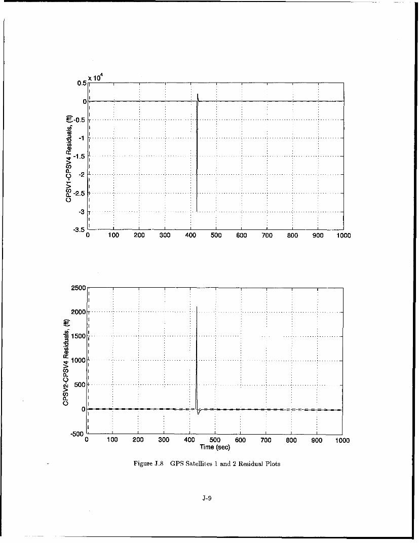
0.1
-- - -- - .. . I . . . .-1. ---- ..... --- -------
-2 ... ..... .. .. . ....... ...1. . .... ... .. .. ....... ... .... . ...
-250
-3.......----...........................
50 ... .. . .. . ------....... . .... ----
0 100 200 300 400 500 600 700 800 900 1000
Fiur J..P aeltsIad2Rsda lt
IJ 9

C/
100
-100 .. . . . -- - - - - . . . .
C20----------- :......--------- - -.... ...-..... --------- - - -
~-400
0 100 200 300 400 500 600 700 800 900 1000Time (sec)
Figure J.9 GPS Satellites 3 and 4 Residual Plots
J-10

Appendix K. Double Difference PNRS Large Cycle Slip on Satellite #4 Results
This appendix contains the results of the 1000 second simulation run of the Double Difference
PNRS filter with a large cycle slip on satellite 4. The plots are in the same order of Appendix G
for direct comparison.
A legend for the presented figures is given below.
Table K.1 Legend for Filter Tuning Plots
Symbol Definition
- Solid Line Mean Error... Dotted Line Mean Error ± True Sigma- - Dashed Line ± Filter Predicted Sigma
K-1

- 0 0 .. . .. . .. .. . . ... . - - - - -. . . . . . . . - - - - - - - - -
I ............
:-5000
-2000.
1~-0000 ....
-5000 I I
0 100 200 300 400 500 600 700 800 900 1000
1im (sec)
Fiur K..ogtd n attd ro lt
100002

2000
0
-2 0 0 0 -.-.---- --. -. ----... ..................... ... ...... ...... ... .. .... ..... ............ .......... .......... ..
0 -4 0 0 0 . .............................. .... .... ....... ........ .......... ........ ............. ..................
S-6 0 0 0 . ..... .. . . . . . . . . . . . . . . . . . . . . . . . . ............... ....................... .........
-8 0 0 0 - - -- --- -- --.. . .. ... ..- ---... .... . . . I.... .. ... .. I... ... ... .... ..... . ... . . . .. . . . .. . . . .. . . . .. . . . . . . . .
-1 0 0 0 0 -.-.----.. ..... ........................... . ............... ............ . . . .............. ...........
-120000 100 200 300 400 Soo 600 700 800 900 1000
5000
0
-10000
-12000
5-000
-2500
' -1000
-0 .... . . . .-15cU
-4 0 0 0 . . . . . . . . -
0 100 200 300 400 500 600 700 800 900 1000Time (sec)
Figure K.2 Altitude and Barometric Altimeter Error Plots
K-3

2 0 x
a)
~010
005.
a) 0.
$DaD. ......... ........................). . ..
.o -0.005 .. ....:. .... - --
a)-0.025
0 100 200 300 400 500 600 700 800 900 1000
X 10-38
a)
a)'D
4 -0- - - - - - - - - - - - - - - - - - -- - - - - - - - - - - - - - - -- - - - - . . . .
020 0 0 0 00 70 80 90 10E - - -- _--- -_-- -- -_ _... .. .... .. .. . .. .. .. .... ._.. .... .. .. . _.. .. .
-4-

__, 250 I ,
•200
2 05 0 . . . .. .. . . . . . . .. . .. . . ..... ..... . . .... . . . . . . . .. .. .. .. .. . . ... ... .. .. .. ... . .. -
2 1 5I 0 . . .. . ... . .. . . ... . .. . .. .. .. ... .. .. .. . .. .. . ... .. . .. . .. :... ... . .. ... .. .. .. .. .. . . .. .. .. .. ... .. . .. .. .. .. . ... . ..
:11150 .......... .............. ..........--- .......... .............. ....... ........... ............-----~10
05.
z -50 I0 100 200 300 400 500 600 700 800 900 1000
30U-,
- 20w.• 10
00)> 0 ...... ...
"-10'0 100 200 300 400 500 600 700 800 900 1000
500
S-500 .......... ........................ ........... 100 200 300 40 ....... ............. 1w S-1 0 0 0 . .. .. . .. .... .. .. . .. .. .. . .. .. .. . .. . .. .. . .. . . . .. . . ....... .. .. . .... .. .. .. ... . . .. . ... .. . .. . . .. . .
o 1 5 0 0 -- - --.. . .. .. .. ... .. .. . ...... ...... . ... .... . .. . .. .. .. .. . .. . ... I --- ---... .. .... .. . .. . .. . . . . .. . . . . .. . .. . . . .
S-2 0 0 0 ------. . ---. .. .. .. --.. .. .. . .. .. . .. .. .. -... .. .. . .. .... . .. .. .. .. . .. .. .. .. .... . . . . .. .. .. ... . . . .. .. .. ..
-25000 10O0 200 300 400 500 600 700 800 900 1000
Time (sec)
Figure K.4 North, West, and Vertical Velocity Error Plots
K-5

-2000
0
w
CL
~-12000
0u -800030 40 0 60 70 0 00 10
0.015
0.01
-0 0005 . . . .... ........ . ... ........
-200
0
-'0.005
-0.005
0 100 200 300 400 500 600 700 800 900 1000Time (sec)
Figure K.5 RRS Range Bias, Range Velocity, and Atmospheric Propagation Delay Error Plots
K-6

-1000
0)
2 -3000 ......... . ...
2 000
-6000 ----
-7000-0 100 200 300 400 500 600 700 800 900 1000
1000
0
E
S-4000 .. ..
a)
> ~ -5000 - - - - - - - - - - - . . . . . . . . . . .. . - - . . . .
co)
-90000 100 200 300 400 500 600 700 800 900 1000
Time (sec)
Figure K.6 GPS Satellites 1 and 2 Phase Ambiguity Error Plots
K-7

1000 I
0
w> ,: -1 0 0 0 .. ... ...... .... ..-. .. . .......... --- --. .... ....
-2 0 0 0 ... -- -- ..... . .... .. .. . -
CI)
-) 4 0 0 0 -- --- .. - .. . -- --.. .. ..... ........ . .... ...
-5000 I0 100 200 300 400 500 600 700 800 900 1000
3.5 X 10
0 ...... .....
0)
-0.50 100 200 300 400 500 600 700 800 900 1000
Time (sec)
Figure K.7 GPS Satellites 3 and 4 Phase Ambiguity Error Plots
K-8

x103.51
3 . . . . . .,. . . . . . . .,. . . . . . .. . . . . . . .. . .. . . . . . . . . .,. . ... . . . - - - . . . . . . . . .. ,. . . . . . . . . . . . . . . ..
a)I2,5 -- - - - -.. . . . . . . . ... . . . . . . . . . . . . . .... . . . . . . .. . . . . . . . . . . . . . .... . . . . . .. . . . . . . . .. .. . . . . . . . . . . .. . . . . .- - - - - -
a)n " 1 .5 t .. . .. . . . .... . . .. . .. . .. . ....- - ---.. . ..... . .. . .. .. . ..... I.. . .. .... . . .. .. . .... .. . . .. ..... . . . . . . . . . . . . . .
>CDQ " 1 .. . . . . . . . . . . . . . . . . . . ... . . . . . . .. - :.. .. . .. . . . . . . . . . . . . . . . ... . . . . . . . . ... . . . . . . . . . ... . . . . . . . . . . . . . . . . . ..-
CD 0 .5 .. . . .. .. .... . .. . .. . . .. . .. . .. . .. ... .. .. . . . .. .. . - -----.. .. .. . . .. ... . . .. . .. ... ... .. . . . .. .. . ..... . . . . . . . . . .
13.5
0
-0.50 100 200 300 400 500 600 700 800 900 1000
X 1043.5.
3g 2.5 .... ..........................
------2 . . . . . . . . . . . . . . . . .... . . ..... .. . . .. .. .. . .... .. . ... .... . .. .. . ...-- ---- -----. .. . .. .. . .. . .. .. . .. .. ..S2.5
a)It 1 .5 - . . .. . .. . .. . .. . .. . .. .. . .. .. . . .. ... . ..... . . . . . .. . . .. .. .. .. .. . . . . .... . .. .. . .... . . .. .. . ... . . .. . .. ...-- -- -
C"o,) 0 .5 t . . . . . . .... . . . . . .. . . .- - - - - - - - - - - . . . . . . . . .. . . . . . . . ... . . . . . . . .. . . . . .. . . . .. . . . . . . . . . . ... . . . . . . .. .. . . . . . . . . .
0-
-0.5 ' I0 100 200 300 400 500 600 700 800 900 1000
Time (sec)
Figure K.8 GPS Satellites 1 and 2 Residual Plots
K-9

x13.5
3 : - -- . .. .. . ... --- --- ... ...... ...
cc1.
CIL
0
-0.50 100 200 300 400 500 600 700 800 900 1000
0.5
0
-0 . I - - - -- - - - - . . . . . . . .. . . .. . . . . . .. . . . . .. . . . . - - - -
co
025 I
-3.50 100 200 300 400 500 600 700 800 900 1000
Time (sec)
Figure K.9 GPS Satellites 3 and 4 Residual Plots
K-10

Appendix L. FDIR Results from Chi-Square Analysis
This appendix contains the plots of the Chi-Square test conducted for Cycle Slip detection,
isolation, and recovery analysis. The results from simulations of the ROPNRS and DDPNRS filters
are presented.
L.1 Chi-Square Test from the ROPNRS Filter
The figures presented consist ,of the single cycle slip simulation on each of the four simulated
satellites and the final figure depicts the multiple cycle slip scenario analyzed for the ROPNRS
filter.
L-1

10x10 7
1
lOj
5 -- -- -- ... .. ............. ..... .......- -----. ....------ ..........
00420 421 422 423 424 425 426 427 428 429 430
cc 5 .........
420 421 422 423 424 425 426 427 428 429 430
X 105
CV) 10 I
cz, . .. . . .. .. . . . . . . . . . - - - -
420 421 422 423 424 425 426 427 428 429 430
Xl10
4L-2

10 x 10 5
S5 .......... ' ............ ...... ............. .......... . ..... . ............. ........... I.........
420 421 422 423 424 425 426 427 428 429 430
x 107
CO
01
420 421 422 423 424 425 426 427 428 429 430
x 10100 2I I
...... ...... - ---.. ........ .................
420 421 422 423 424 425 426 427 428 429 430
x 104
00 II-420 421 422 423 424 425 426 427 428 429 430
Time (sec)
Figure L.2 Chi-Square Plots of Individual Residuals for Cycle Slip on Satellite #2
L-3

x 106
420 421 422 423 424 425 426 427 428 429 430
X 106
c 10
420 421 422 423 424 425 426 427 428 429 430
X 106i-0 10 I
420 421 422 423 424 425 426 427 428 429 430
X 100
CO,
c 1 0, 5 --- -- - -- - --- - -- --
0•420 421 422 423 424 425 426 427 428 429 430
x 10,
CO
Time (sec)
Figure L.3 Chi-Square Plots of Individual Residuals for Cycle Slip on Satellite #3
L-

x 10
1=" II I
420 421 422 423 424 425 426 427 428 429 430
x WSI I I I I I I I I
43 - . ....... . ....----------- -
00 5420 421 422 423 424 425 426 427 428 429 430
x 105j3I I I I I I I I
CO, -- ---... .. ----- ..."• iii ........ l ....... .. .. ........ ... ... ii
00
420 421 422 423 424 425 426 427 428 429 430
x 108
0,
420 421 422 423 424 425 426 427 428 429 430Time (sec)
Figure L.4 Chi-Square Plots of Individual Residuals for Cycle Slip on Satellite #4
L-5

x 10 7
CD1 ," 1 0 ---------- .. ... .. ... .. ..... .. .... " ........... ..........----------. ............ ..........!. .........
• " 5 - - - - -. .... .. . . . . ... . . . . . . . . . . . . . . . .. . . . . . . . . ... . . . .. .. . . . .. . . . .. . . . . . . . .
I I" II I
420 421 422 423 424 425 426 427 428 429 430
x 107S4 I I I . . .
420 421 422 423 424 425 426 427 428 429 430
X 107oy)2 -CO•
" ------ ..... ....-----------...... .. ..................
420 421 422 423 424 425 426 427 428 429 430
> 1 04 07
CO I
.4 0 I-j
420 421 422 423 424 425 426 427 428 429 430Time (sec)
Figure L.5 Chi-Square Plots of Individual Residuals for Multiple Cycle Slip Scenario
L-6

L.2 Chi-Square Test from the DDPNRS Filter
The figures presented consist of the single cycle slip simulation on each of the four simulated
satellites and the final figure depicts the multiple cycle slip scenario analyzed for the DDPNRS
filter.
L-7

x 107-10-CD
CO
00420 421 422 423 424 425 426 427 428 429 430
x 109CM 4
CO
• 2 --------. . . . .... ... .... . . . .... . . .. . . .. . .. . .. .. . .. . .. .. . .. ...-
0.420 421 422 423 424 425 426 427 428 429 430
x 10s
S2 ........... .................---... ...........--- -- .....
cc 2
0
420 421 422 423 424 425 426 427 428 429 430
X 104
CO
LD
"•0 0420 421 422 423 424 425 426 427 428 429 430
Time (sec)
Figure L.6 Chi-Square Plots of Individual Residuals for Cycle Slip on Satellite #1
L-8

x10
-. - - - ... -- ----
40 42 42 2 z2 2 2 2 2 2 3
420 421 422 423 424 425 426 427 428 429 430
xlo5JExc' 15I
42C2D2 23 44 45 46 42 2 2 3'610 ~ ~ ~ ~ ~ ~ ~ ~ ~ Tm ....... se .......-c)-------------
FiueccCiSur lt fIdvda RsdasfrCceSi nStlie#
... . ..... .. ..... ..L...

x 106SI I I I I I I I Ij
U46 ----------
I' I I I I i
420 421 422 423 424 425 426 427 428 429 430
x 106CY10,. . . ....... . . .
oL420 421 422 423 424 425 426 427 428 429 430
X 107
S01420 421 422 423 424 425 426 427 428 429 430
X 105
U)4 -- ----------..... .....
m= 2 .........-- .......... :.......... :.......... ......... .. .. .............. :.......... :..........
420 421 422 423 424 425 426 427 428 429 430Time (sec)
Figure L.8 Chi-Square Plots of Individual Residuals for Cycle Slip on Satellite #3
L-10

- 10 X 107
420 421 422 423 424 425 426 427 428 429 430
x 10
CJO
C,,
01
420 421 422 423 424 425 426 427 428 429 430X 107
043420 421 422 423 424 425 426 427 428 429 430
x 108
cc 5 o ' 2 .. . .. ... . .. . ... ........ ........... ............ ..........
0
420 421 422 423 424 425 426 427 428 429 430
Time (sec)
Figure L.9 Chi-Square Plots of Individual Residuals for Cycle Slip on Satellite #4
b-il

0 0 I III420 421 422 423 424 425 426 427 428 429 430
X10
=0I
0420 421 422 423 424 425 426 427 428 429 430
X 107
Ir I420 421 422 423 424 425 426 427 428 429 430
X 10o7
-420 421 422 423 424 425 426 427 428 429 430Time (sec)
Figure L.10 Chi-Square Plots of Individual Residuals for Multiple Cycle Slip Scenario
L-12

Appendix M. Lack of Independence of GPS Satellite Differencing Proof
This proof will show, for the case of using GPS satellite combinations of SV1 - SV4, SV2 -
SV4, and SV3 - SV4, where SV stands for Space Vehicle, that independence between these
measurement combinations does not exist.
First, we assume that each measurement error can be represented by a Gaussian random
variable, m, with the following statistics:
E[m,] = 0 (M.1)
and
E[mn] = M, (M.2)
where x represents the number of the satellite measurement. It is assumed that the noises in all
original (undifferenced) measurements are independent of each other. With this assumption, the
following is true:
[m3] ifx=y=zE[m.,my mz] ]M3
0 otherwise
Taking the fourth satellite measurement, M 4 , as a base measurement, the following difference pairs
are available: m 1 - M 4 , m 2 - M 4 , m 3 - M 4 . For independence between measurements to be proven,
the following relation must be true:
E[(m -- m4)(m2 - m4)(m3 - M 4 )] =- E[mi - m 4]E[m 2 - in 4 ]E[m3 - M4] (M.4)
Combining the different quantities on the left hand side of Equation (M.4) produces:
2 _ 2 2 - 3
E[mlm 2 mi 3 - mnlim3 m 4 -M 42 m 3 m 4 + m 3 m2 - ml m 2 m 4 + mlm2 + m 2 m2 - m3] (M.5)
M-1

Using the distributive property of expected values, Equation (M.5) becomes:
E[mlm 2m3] - E[mIm3m 4] - E[m 2m 3m 4 ] + E[mam3]
-E[mim 2m 4] + E[mjm4] + E[m2m4] - E[m ] (M.6)
Invoking the independence assumption of Equation (M.3) changes Equation (M.6) to become:
-E 4~• (M.7)
Using the distributive property of expected values on the right hand side of Equation (M.4) pro-
duces:
[E[mi] - E[m4]] [E[m 2] - E[m4]] [E[m3] - E[m4]] (M.8)
From the zero mean assumption of Equation (M.1), Equation (M.8) becomes zero. Because of
the conditions set forth in Equation (M.4) were not met, the independence of the three satellite
measurement combinations does not exist.
M-2

Bibliography
1. Britting, Kenneth R. Inertial Navigation Systems Analysis. New York: Wiley-Interscience,1971.
2. Canadian GPS Associates. Guide to GPS Positioning . ISBN: 0-920-114-73-3, Fredericton,New Brunswick: University of New Brunswick Graphic Services, May 1987.
3. Carlson, Neal and Stanton Musick. User's Manual for a Multimode Simulation for OptimalFilter Evaluation (MSOFE). AFWAL-TR-88-1138, Wright-Patterson AFB OH: Avionics Lab,AFWAL/AARN-2, April 1990.
4. Cox, D. B. "Integration of GPS with Inertial Navigation Systems," Global Positioning System.Papers Published in Navigation, Volume 1:144-153, The Institute of Navigation, Alexandria,VA 22314, 1980.
5. Knudsen, L. Performance Accuracy (Truth Model/Error Budget) Analysis for the LN-93 Iner-tial Navigation Unit. Technical Report, Litton Guidance and Control Systems, January 1985.DID No. DI-S-21433 B/T:CDRL No. 1002.
6. Lachapelle, Gerard, M. E. Cannon and G. Lu. "High-Precision GPS Navigation with Emphasison Carrier Phase Ambiguity Resolution," Marine Geodesy, 15: 253-269 (1992)
7. Lachapelle, Gerard and M Casey. "Use of Phase Data for Accurate Differential GPS KinematicPositioning," Proceedings of Position, Location, and Navigation Symposium. 393-398. NewYork: IEEE Press, 1986.
8. Hansen, Neil P. Incorporating Carrier Phase GPS Measurements into the CHAPS ExtendedKalman Filter. Unpublished Report to 46th GTS/TGFGXR, Holloman AFB, New Mexico. 03May 1994.
9. Hansen, Neil P. Incorporation of Carrier Phase Global Positioning System Measurementsinto the Navigation Reference System for Improved Performance. MS Degree Thesis,AFIT/GE/ENG/93D-40. School of Engineering, Air Force Institute of Technology (AU),Wright-Patterson AFB OH, December 1993 (AD-A274136).
10. Hooser, Michael. Director Research and Development, Central Inertial Guidance Test Facility,Holloman AFB, NM. Telephone Interview. 20 July 1994.
11. Johnson, Gregory B. Closed-Loop Performance of GPS Aided INS. MS Degree Thesis,AFIT/GE/ENG/89D-19. School of Engineering, Air Force Institute of Technology (AU),Wright-Patterson AFB OH, December 1989 (AD-B139003).
12. Lewantowicz, Zdzislaw H. and Danny W. Keen. "Graceful Degradation of GPS/INS Perfor-mance With Fewer Than Four Satellites," The Institute of Navigation, National TechnicalMeeting (January 1991).
13. Mader, Gerald L. "Dynamic Positioning Using GPS Carrier Phase Measurements,"Manuscripta Geodaetica, 11: 272-277 (1986).
14. Matlab. Version 4.1. Computer software. The MathWorks, Inc. 24 Prime Park Way, Natick,MA 01760. June 1993.
15. Maybeck, Peter S. Stochastic Models, Estimation, and Control. Volume 1. New York: AcademicPress, Inc., 1979.
16. Maybeck, Peter S. Stochastic Models, Estimation, and Control. Volume 2. New York: AcademicPress, Inc., 1982.
17. Maybeck, Peter S. Stochastic Models, Estimation, and Control. Volume 3. New York: AcademicPress, Inc., 1982.
BIB-1

18. Maybeck, Peter S. Professor of Electrical Engineering, Air Force Institute of Technology,Wright-Patterson AFB, NM. Personal Interview. 12 September 1994.
19. Menke, Timothy E. and Peter S. Maybeck. "Sensor/Actuator Failure Detection in the VISTAF-16 by Multiple Model Adaptive Estimation," Proceedings of the American Control Confer-ence, San Francisco, June 1993 (1993).
20. Mosle, William B. Detection, Isolation, and Recovery of Failures in an Integrated NavigationSystem. MS Degree Thesis, AFIT/GE/ENG/93D-28. School of Engineering, Air Force Instituteof Technology (AU), Wright-Patterson AFB OH, December 1993 (AD-A274056).
21. Mosle, iLt William B. Aircraft GPS Integration Element Officer, 46th Guidance TestSquadron, Holloman AFB, NM. Telephone Interview. 18 July 1994.
22. Musick, Stanton H. PROFGEN - A Computer Program for Generating Flight Profiles. Techni-cal Report, Air Force Avionics Laboratory, WPAFB, Ohio, November 1976. AFAL-TR-76-247,DTIC ADA034993.
23. Negast, William Joseph. Incorporation of Differential Global Positioning System MeasurementsUsing an Extended Kalman Filter for Improved Reference System Performance. MS DegreeThesis, AFIT/GE/ENG/91D-41. School of Engineering, Air Force Institute of Technology(AU), Wright-Patterson AFB OH, December 1991 (AD-A243742).
24. Nielsen, Robert L. Development of a Performance Evaluation Tool (MMSOFE) for the De-tection of Failures with Multiple Model Adaptive Estimation (MMAE). MS Degree Thesis,AFIT/GE/ENG/93S-37. School of Engineering, Air Force Institute of Technology (AU),Wright-Patterson AFB OH, September 1993 (AD-A274218).
25. Riggins, Lt Col Robert N. Assistant Professor of Electrical Engineering, Air Force Institute ofTechnology, Wright-Patterson AFB, OH. Personal Interview. 2 May 1994.
26. Snodgrass, Faron Britt. Continued Development and Analysis of an New Extended KalmanFilter for the Completely Integrated Reference Instrumentation System (CIRIS). MS The-sis, AFIT/GE/ENG/90M-5. School of Engineering, Air Force Institute of Technology (AU),Wright-Patterson AFB OH, March 1990 (AD-A220106).
27. Snodgrass, Capt Britt and Capt John Raquet. Project Officers of The CIGTF High Accu-racy Post-processing Reference System, 46th Guidance Test Squadron, Holloman AFB, NM.Personal Interview. 17 March 1994.
28. Solomon, Joseph K. Development of the Extended Kalman Filter for the AdvancedCompletely Integrated Reference Instrumentation System (CIRIS). MS Degree Thesis,AFIT/GE/ENG/89M-08. School of Engineering, Air Force Institute of Technology (AU),Wright-Patterson AFB OH, March 1989 (AD-A206083).
29. Stacey, Richard D. A Navigation Reference System (NRS) Using Global Positioning System(GPS) and Transponder Aiding. MS Degree Thesis, AFIT/GE/ENG/91M-04. School of En-gineering, Air Force Institute of Technology (AU), Wright-Patterson AFB OH, March 1991(AD-A238890).
30. Talbot, Nicholas C. "High-Precision Real-Time GPS Positioning Concepts: Modeling andResults," Global Positioning System. Papers Published in Navigation, Volume IV:221-235,The Institute of Navigation, Alexandria, VA 22314, 1993.
31. Vasquez, Juan R. Detection of Spoofing, Jamming, or Failure of a Global Positioning System(GPS). MS Degree Thesis, AFIT/GE/ENG/92D-37. School of Engineering, Air Force Instituteof Technology (AU), Wright-Patterson AFB OH, December 1992 (AD-A259023).
BIB-2

32. Wong, R. V. C., K. P. Schwarz, and M. E. Cannon. "High-Accuracy Kinematic Positioning byGPS-INS," Global Positioning System. Papers Published in Navigation, Volume IV:237-250,The Institute of Navigation, Alexandria, VA 22314, 1993.
BIB-3

Vita
Second Lieutenant Brian J. Bohenek was born to Mr. and Mrs. Joseph Bohenek on 9
December 1971 in Scranton, Pennsylvania. Upon graduation from Scranton Central High School
in 1989, Brian began his undergraduate studies in Electrical Engineering at Wilkes University in
Wilkes-Barre, Pennsylvania. While at Wilkes, he enrolled in the Air Force Reserve Officer Training
Corps (ROTC) to pursue his dream of becoming an Air Force Officer. Wilkes also provided Brian
the opportunity to meet his fianc6, Miss Linda Wiernusz of Wilkes-Barre Township, Pennsylvania.
Upon graduation from Wilkes in May 1993, Brian was commissioned as a Second Lieutenant in
the United States Air Force and recognized as a Distinguished Graduate from Air Force ROTC.
In June 1993, Brian was called onto active duty in the Air Force to continue his previous career
as a student at the Air Force Institute of Technology (AFIT) Wright-Patterson AFB, Ohio. While
at AFIT, he earned a Masters of Science Degree in Electrical Engineering with a concentration
in navigation systems. Following graduation from AFIT in December 1994, the seemingly endless
academic career of Brian's was temporarily put on hold so he could become a member of the 746th
Test Squadron, Holloman AFB, New Mexico. While working at Holloman, Brian worked as a Flight
Test Engineer and prepared for his wedding to his fianc6, Linda.
Permanent address: 906 Monroe AvenueScranton, PA 18510
VITA- I

R~?CR C, OCUMENTATION PACEH.
cc!Iec-.:cr 'Tc. luO swg:east cns -or recu-n Zhis ourcer. -zr PlashingTon HeacurT.?rs ýe' ces, D'recC-r3te eT-eT"tPTh'ICSYC '~' ' rs~onDavis Hcr',.. -C:24, Amryaton, 22322-302, ean to tne Office of Mna~emernet ,r'd 3udger, Paervorl< Reduction C '- 0 tP ::n
1. AGENCY USE ONLY (Leave blank) 2. REPORT DATE 3. REPORT TY(PE ANO DATES 3~EDecember 1994 J Master's Thesis
4. TITLE AND SUBTiTL! 5. FUNZ:41G AU'IUSERSTHE ENHANCED PERFORMANCE OF AN INTEGRATEDNAVIGATION SYSTEM IN A HIGHLY DYNAMICENVIRONMENT i
6. AUTHCR(S)
Brian J. Bohenek
7.PEIRFIRMING ' .RGAMIZAT;0N '4ANE"'S) AND ADDRESS(CES) 2.?E2~'G2AI2TO
Air Force Institute of Technology, WPAFB OH 45433-6583 REP'A' t *LNSE
AFIT/GE/ENG/94D-o 1
9. SPONSCRiNG, MONITORING AGENCY NAME(S) AND ADORESS(ESi 0 P~S ~MNTRN746th Test Squadron AGENCY AZEr.RT AIUMSEAR
* 1644 Vandergrift Rd.* Holloman AFB, NM 88330-7850
11. SUPPLEMIENTARY NOTES
12a. OlSiRIBUT(ON/AVAILASIUITY STATEMIENT .12b. DIST;RIS>O;ý 'CCE:
Distribution Unlimited
13. ABSTRAC7 .,maximumn200 words)
For the U. S. Air Force to maintain an accurate and reliable Navigation Reference System (NRS) with Carrier-* Phase Global Positioning System (CPGPS) measurements, it must develop an accurate and robust NRS in the
face of cycle slips caused by highly dynamic maneuvers. This research investigates the implementation of a* double differencing between receivers/satellites scheme to improve the accuracy of current NRS models. The
removal of the "perfect Doppler velocity aiding measurements" (a very poor assumption of past research) wascompleted with stable and accurate results. The double differencing implemented showed improvement in theaccuracy of the NR.S. An investigation of two Failure Detection, Isolation, and Recovery (FDIR) algorithms forlarge cycle slip failures is conducted. The two FDIR techniques are the Chi-Square test and a Multiple ModelAdaptive Estimator (MMAE). The FDIR results show that a Chi-Square test as a stand-alone algorithm canwork accurately for detection and isolation of failures with an accurate and reliable recovery algorithm. The 1iMMAE algorithm as conjectured seems to be the best FDIR technique to handle single and multiple cycle slipsaccurately and reliably.
( 14. SUBJECT TERMS 115. NUMBER OFPAECarrier-Phase GPS, Cycle Slip, Global Positioning System, GPS, 245Extended Kalman Filter, Navigation Reference System, MSOFE '16. PRICE CODE
17. SECURITY CLASSIFICATION 118. SECURITY CLASSIFICATION 19. SECURITY CLASSIFICATION 20. LIMITATION OF ABSTRACTOREOTOF THSPG FASRC
UNCLASSIFIED UNCLASSIFIED UNCLASSIFIED UL
NSN 7540-01-280-5500 Standard Form .298 (Rev. 2-89)Prescribed by ANSi Sta. Z39-18'98-IC2