I DTIC

~OF

DESIGN OF WATER TUNNEL TO MEASUREWALL PRESSURE SIGNATURES DUE TO

TUNNEL BLOCKAGE AND WAKE EFFECTS

THESIS

Kurt A. LautenbachCaptain, USAF

AFIT/GAE/AA/88D-20

DEPARTMENT OF THE AIR FORCE

AIR UNIVERSITY

AIR FORCE INSTITUTE OF TECHNOLOGY

Wright-Patterson Air Force Base, Ohio

DISTRItUnlON STATE:/-l-rf A

ApprnvIi for public

DISCLAIMER NOTICE

THIS DOCUMENT IS BEST QUALITYPRACTICABLE. THE COPY FURNISHEDTO DTIC CONTAINED A SIGNIFICANTNUMBER OF PAGES WHICH DO NOTREPRODUCE LEGIBLY.

AFIT/GAE/AA/88D-20

DESIGN OF WATER TUNNEL TO MEASUREWALL PRESSURE SIGNATURES DUE TOTUNNEL BLOCKAGE AND WAKE EFFECTS

THESIS

Kurt A. LautenbachCaptain, USAF

AFIT/GAE/AA/88D-20

DTICMAR3 0o91

Hq

Approved for public release; distribution unlimited

AFIT/GAE/AA/88D-20

DESIGN OF WATER TUNNEL TO MEASURE WALL PRESSURE SIGNATURES

DUE TO TUNNEL BLOCKAGE AND WAKE EFFECTS

THESIS

Presented to the Faculty of the School of Engineering

of the Air Force Institute of Technology

Air University

In Partial Fulfillment of the

Requirements for the Degree of

Master of Science in Aeronautical Engineering

Acoession ForI4TIS GPA&I

DTIC TAFUn aat c,-i e d

Kurt A. Lautenbach Ju tLt, tt o n_-

Captain, Unites States Air Force

December 1988

Approved for public release; distribution unlimited

Preface

In this study, a water tunnel with a ten inch square

test section was designed and constructed for the purpose of

taking wall pressure signature data. This data is useful in

analyzing solid blockage and wake blockage of the tunnel and

can be collected without a priori knowledge of model

geometry even in cases with separated flow. Previous

studies in wind tunnels have shown that this technique

allows for accurate measurements on models which are large

in relation to the tunnel test section size. This is the

*first time such a study has been attempted in a water

tunnel. Eventually, I hope that development of this

technique in water leads to an aerodynamic test facility

where indirect force measurements can be made simultaneously

with excellent flow visualization.

I now take this opportunity to thank Maj L. Hudson for

his guidance during this project. I also thank Professor H.

Larson , Lt Col P. King and Dr. A. Nejad for their many

helpful suggestions in the design of the hardware involved.

Finally, I especially thank my wife Joanne for filling in

for me at home while I was neglecting my family in the

interests of higher education.

Kurt A. Lautenbach

ii

Table of Contents

Page

Preface .......... ......................... ii

List of Figures ......... .................... iv

List of Tables ........ .................... vii

List of Symbols ........ .................... .. viii

Abstract ......... ........................ x

I. Introduction ........ ................ 1

II. Literature Review ....... .............. 7

III. Tunnel Flow Analysis ... ............ . 18

IV. Design of Water Tunnel ... ........... . 33

Primary Requirements ......... 33Description of Present Facility . ... 33Modifications to Present Facility . 36Design of Ten Inch Square Water Tunnel 37

Test Section ... ........... .. 37Downstrean Duct ... .......... .. 40Upstream Diffuser and Stilling Tank 42Nozzle .... .............. . 44Instrumentation ... .......... .. 44

V. Conclusions and Recommendations ........ .. 49

Appendix A: Water Tunnel Component Drawings ..... . 54

Appendix B: FORTRAN Program for Calculation of VelocityField Around Sphere in Rectangular Tunnel 92

Appendix C: Acrylic Window Structural Analysis . . .. 95

Appendix D: Nozzle Design ..... .............. 102

Bibliography .i.................... 110

Vita ... .......... ............... 114

List of Figures

Figure Page

1. Wall Pressure Signature Decomposition ...... . 12

2. Location of Line Sources and Sinks .. ........ .. 13

3. Image Array and Source Sheet ... ........... .. 14

4. Coordinates for Sphere in Tunnel Imaging ..... . 18

5a. Pressure Coefficient, Wall Pressure SignaturePredicted, Wake Neglected ... .......... .. 22

5b. Pressure Coefficient, Wall Pressure SignaturePredicted, Wake Included .. .......... .. 25

6. Predicted Wall Pressure Signaturefrom Five Inch Sphere Model .. ......... .. 26

7a. Pressure Differences Along Window Centerline,Wake Neglected ..... ............... . 27

7b. Pressure Differences Along Window Centerline,Wake Included ..... ................ . 29

8a. Pressure Coefficient on Test Section Wall,Wake Neglected ..... ............... . 30

8b. Pressure Coefficient on Test Section Wall,Wake Included ..... ................ . 31

9a. Free Stream Pressure Coefficient Contours,Wake Neglected ..... ............... . 31

9b. Free Stream Pressure Coefficient COntours,Wake Included ..... ................ . 32

10. Flow Diagram ...... ................... . 35

11. Isometric View, Water Tunnel Assembly ...... . 55

12. Isometric View, Diffuser .... ............. . 56

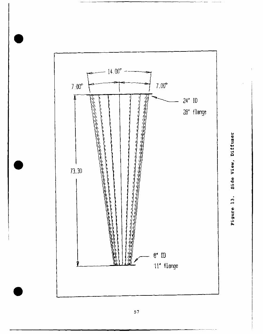
13. Side View, Diffuser .... ............... . 57

iv

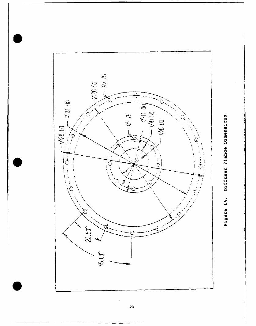
14. Diffuser Flange Dimensions ... ............ 58

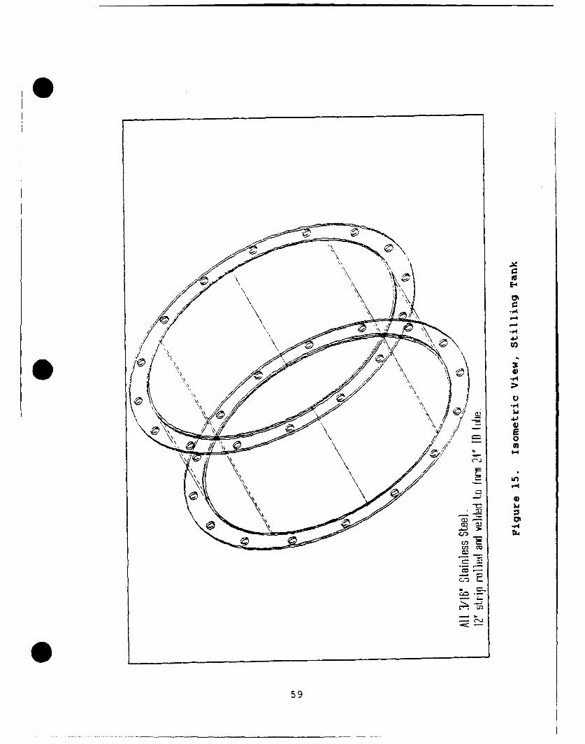
15. Isometric View, Stilling Tank .. .......... 59

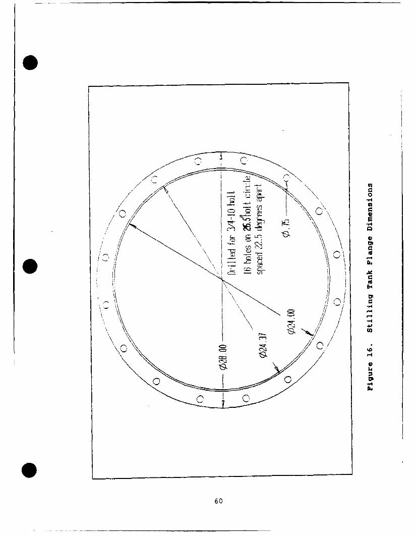
16. Stilling Tank Flange Dimensions . ......... 60

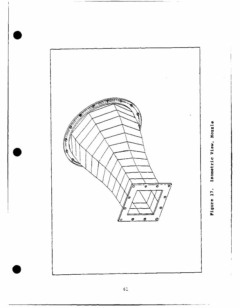
17. Isometric View, Nozzle ..... .............. 61

18. Isometric View, Test Section Assembly . ...... 62

19. Isometric View, Test Section Flange ....... 63

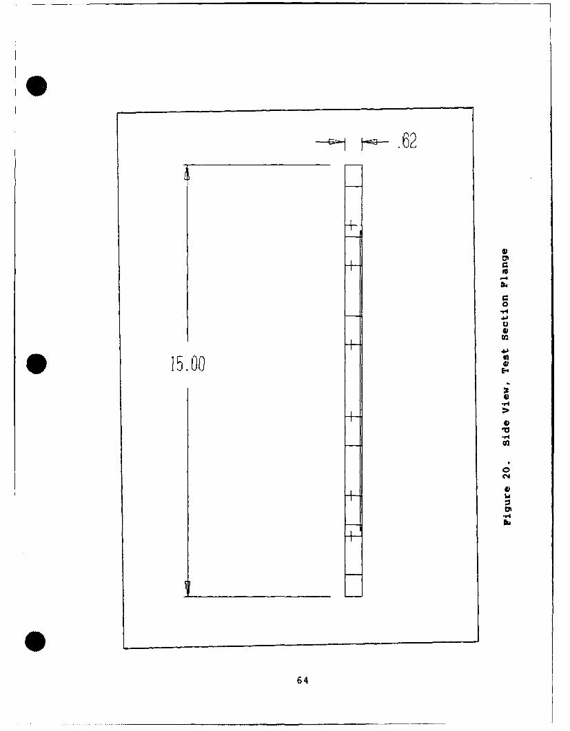
20. Side View, Test Section Flange .. .......... 64

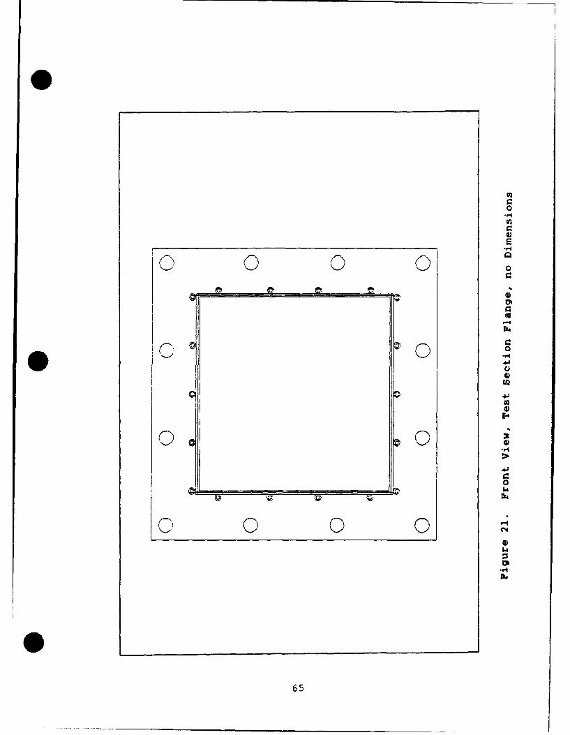
21. Front View, Test Section Flange, no Dimensions 65

22. Front View, Test Section Flange, with Dimensions 66

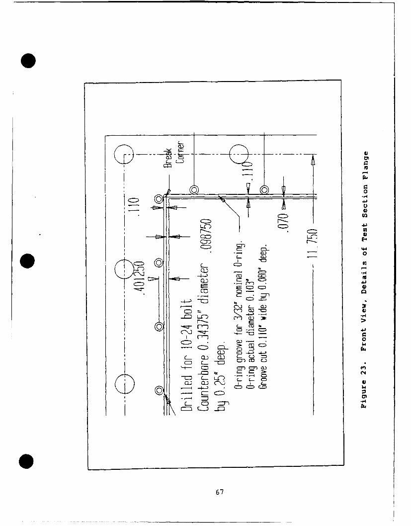
23. Front View, Details of Test Section Flange . ... 67

24. Isometric View, Test Section Ceiling/Floor . ... 68

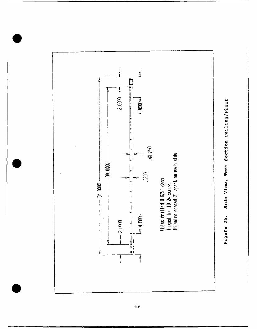
25. Side View, Test Section Ceiling/Floor . ...... 69

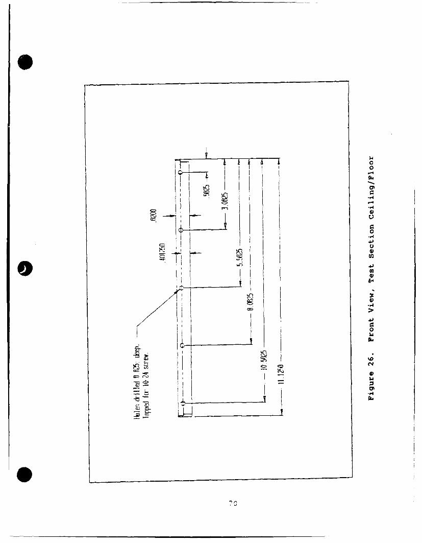
26. Front View, Test Section Ceiling/Floor ...... . 70

27. Top View, Test Section Ceiling/Floor ........ .. 71

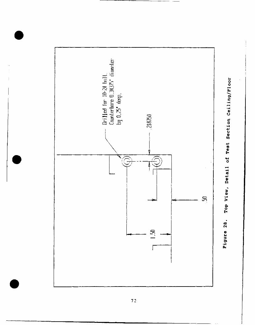
28. Top View, Detail of Test Section Ceiling/Floor 72

29. Isometric View, Test Section Corner Brace . ... 73

30. Front View, Test Section Corner Brace . ...... 74

31. Top View, Test Section Corner Brace . ....... 75

32. Side View, Test Section Corner Brace ........ .. 76

33. Isometric View, Test Section Acrylic Window . . 77

34. Front View, Test Section Acrylic Window ..... 78

35. Side View, Test Section Acrylic Window ...... . 79

36. Top View, Test Section Acrylic Window ...... 80

37. Top View, Detail of Acrylic Window ......... 81

38. Isometric View, Pitot Tube Rake . ......... 82

v

39. Top View, Pitot Tube Rake ... ............ 83

40. Isometric View, Downstream Square Duct ...... . 84

41. Front View, Downstream Square Duct Flange . . .. 85

42. Isometric View, Adapter Assembly .......... . 86

43. Front View, Adapter Large Round Flange ...... . 87

44. Front View, Adapter Small Round Flange ...... . 88

45. Front View, Adapter Reinforced Rubber Diaphragm 89

46. Isometric View, Adapter Round Diaphragm Clamp 90

47. Front View, Adapter Square Diaphragm Clamp . . .. 91

48. Cross Section of Finite Element Model of Flat Plate 99

49. Cross Section of Finite Element Model of Window 100

50. General Longitudinal Section of Nozzle ....... . 103

51. Cross Sections of Nozzle at Evenly SpacedLongitudinal Stations ... ............ 108

vi

List of Tables

Table Page

1. Physical Properties of Acrylic PLastic ...... . 89

2. Stress Analysis of Thin Acrylic Plate ...... 92

vii

List of Symbols

A vector

b Model span, or width

b Line source span5

B Tunnel width, or nozzle width

C Pressure coefficientp

E Young's modulus [psi]

0 Cylindrical coordinate angle from y-axis

or Perturbation velocity potential

P Velocity potential, or spherical coordinate angle

H Tunnel height

* r Surface of ?

F1 Boundary surface of ) where u is known

F2 Boundary surface of 0 where q is known

L Nozzle length

P Doublet strength

M Generalized nozzle radius

n Unit normal vector

P Pressure, or point

psi Pounds per square inch

psig Gage or differential pressure, pounds per square inch

q au/an, normal derivative of u

q Known value of q on F2

Qs Source or sink strength for solid blockage

viii

Qw Source or sink strength for wake blockage

r Cylindrical coordinate, radius from x-axis,or in nozzle, generalized cylindrical radius

r Generalized non-dimensional radius in nozzle

R Spherical coordinate, radius from origin,or in nozzle, cylindrical coordinate radius from x-axis

R Radius of spheres

a Stress [psi]

O Spherical coordinate, angle from x-axis,

or in nozzle, smaller of angle from y-axis or z-axis

0 Spherical coordinate angle

t thickness

u Local velocity, or velocity potential

u Known value of u on F

Au Perturbation velocity

U Free stream velocity

U Free stream velocity

o Domain for volume integral

w integrating factor, weighting function

x Rectangular coordinate, direction of free stream flow

x Non-dimensional x

y Rectangular coordinate, width

z Rectangular coordinate, height

ix

AFIT/GAE/AA/88D-20

Abstract

I

This thesis describes the design and construction of a

new test section for the AFWAL Aero Propulsion Lab six-inch

water tunnel in building 18. The new test section has a

ten-inch square cross section and is designed to measure

wall pressure signatures caused by solid and wake blockage

of the flow due to the separation bubble which forms around

bluff bodies immersed in the flow. The wall pressure

signature for a spherical model is predicted. Applications

of the method and associated requirements for

instrumentation are discussed. , \

x

DESIGN OF WATER TUNNEL TO MEASURE WALL PRESSURE SIGNATURES

DUE TO TUNNEL BLOCKAGE AND WAKE EFFECTS

I. Introduction

Water Tunnels are often used to provide flow

visualization data which is analogous to the air flows

studied in low speed wind tunnel experiments. However,

force and pressure data are generally not collected in water

tunnel experiments due to the complexity of obtaining and

mounting waterproof pressure transducers and force balances

compatible with the small models and fluid speeds typically

used. Typical flow velocities in flow visualization studies

reduce the Reynold's number to a laminar flow region.

Nonetheless, information concerning the vorticular nature of

the flow is considered of extreme utility in comparison to

full scale behavior. Indeed, excellent agreement has been

observed between water tunnel experimental results and

flight test results in many cases involving separated vortex

flows and complex vortex interaction [7:6-7].

In this study, a water tunnel is used which has had a

new test section designed to resemble a typical wind tunnel

test section. A water tunnel is distinguished from a water

channel in that the channel has a free surface between the

water and air, and partially or fully submerged models are

1

0 tested usually for marine applications. In an experiment

involving a free surface, gravity forces are important and

the Froude number must be considered [7:5]. In a low speed

wind tunnel and in this study, the model is fully immersed

in the fluid and no free surface is involved. The

predominant forces present are viscous and inertial,

therefore Reynold's Number is the appropriate measure of

model similarity for scaling purposes.

It has long been recognized that the flow about a body,

particularly an aircraft, in a wind or water tunnel is not

the same as the flow about the same body in an unconfined

space. The difference between the two flows is not due to

the fact that in actual flight an aircraft moves through

essentially still fluid while in a test tunnel a moving

fluid flows around a stationary body. Instead, the

difference is because streamlines in a closed test section

tunnel are not free to displace away from the body due to

the presence of tunnel walls. The difference between the

wall constrained case and the infinite field case is further

complicated by the effect of the boundary layer on the

tunnel walls, viscous wake, compressibility, and a few other

factors as well [29:chap 6]. Except for compressibility, it

is expected that these effects are not unique to wind

tunnels and could be observed in a water tunnel.

It is common knowledge that all of the above mentioned

* tunnel flow effects cause inaccuracy in experimental

2

measurements, and that these inaccuracies may be avoided by

using models which are small in comparison to the tunnel

test sections. Unfortunately, small models are difficult to

instrument and difficult to build accurately. Further, they

must be tested at larger velocity for the Reynold's number

to match the full scale case and large velocity increases

the Mach number on the model with the result that complete

flow similarity is often impossible to maintain between the

two cases. From the point of view of obtaining accurate

data, the ideal case is to test on a full scale model. This

is prohibitively expensive in both construction and

operation. Thus we are faced with the necessity of using

* rather larger models than the ideal for a given tunnel

facility, and then calculating corrections to the measured

pressure or force data.

Recent wind tunnel experimenters have developed methods

to use wall pressure signature data to estimate tunnel

blockage, estimate wall interference, analyze wake and

vortex flows, and calculate compressibility effects

[27]. This research will utilize flow pressure signatures

on the water tunnel walls to analyze the flow properties.

From this signature, the flow past the body can be

computationally modeled. Due to the preliminary nature of

this study, potential flow theory is used for the flow

modeling, but more complicated theories are equally

applicable. Even in cases where a large separation bubble

3

0surrounds the model, the flow outside the separation bubble

and away from the small boundary layer on the tunnel wall is

essentially potential flow, thus it should be possible to

calculate pressures along a separation bubble or even on the

model itself starting only with wall pressure signature

data. It is also possible to make predictions of the wall

pressure signatures based on either model geometry or based

on separation bubble geometry as observed in flow

visualization experiments which are well established as

water tunnel research techniques [7,32].

The long term objective of this research is to develop

the use of wall pressure signature measurement in a wind

tunnel while also developing a potential flow computer model

of the flow in the tunnel. This will enable the calculation

of pressures on the model with fairly simple experiments

since the model will not necessarily be instrumented as

models generally are for wind tunnel experiments with

pressure ports on the model and complex force measuring

mounting systems. Instead, the instrumentation will be

associated with the tunnel test section only, and will

remain the same for different models. However, the

reduction of the water tunnel wall pressure signature data

will be fairly complex.

The computation method which is most applicable to this

research is known variously as paneling theory, boundary

0 element method, boundary integral equation method, boundary

4

integral solution, and other similar names [4:46]. One of

the features of this method which distinguishes it from

finite elements methods is that only the boundary surface of

the domain of interest is discretized, rather than

discretization of the entire domain. According to Brebbia

[4:1], the boundary element method involves smaller matrix

equations and produces less numerical error than would a

finite element formulation of the same problem.

Since the experimental portion of this investigation

is to be accomplished in a water tunnel, it should be a

straight forward task to obtain flow visualization studies

to verify the computed results. Eventually, a method could

* be developed to make corrections to flow visualization

studies to account for the presence of the water tunnel

walls just as methods have already been developed to account

for the difference in measured forces on models in a free

stream and in a flow confined to a wind tunnel.

The six inch water tunnel located at Wright-Patterson

Air Force Base, Ohio, Building 18 ,room 23 is the designated

facility for the experimental portion of this thesis.

Arrangements to use this facility have been made through the

sponsor of this research, Dr. Abdollah S. Nejad of Air Force

Wright Aeronautical Laboratories, Aero Propulsion

Laboratory, Experimental Research Branch. Renovations to

the test section of the water tunnel have been designed and

constructed. Preliminary instrumentation available consists

5

of manometers to measure static pressure on the water tunnel

test section walls and dynamic pressure upstream of the test

section and at various cross sections of the test section.

Flow visualization capabilities consist of both dye and air

bubble injection systems.

6

II. LITERATURE REVIEW

The recent literature concerning tunnel corrections

calculated from wall pressure measurements in closed

solid-walled wind tunnels assuming incompressible flow was

extensively reviewed. No like material was found concerning

water tunnels. There is a large body of knowledge

concerning wall pressure measurements in transonic flow

facilities, ventilated wall (boundary layer control and

streamline control) tunnels, and flexible adaptive wall wind

tunnels which is similar in some ways to the present subject

but not applicable to this research. In addition to the

recent material concerning wall pressure measurements, this

literature review also presents an overview which points out

the major historical trends in this type of research and the

approximate period in which the different types of wind

tunnel correction methods were developed. Although the

major theme of this research is to take indirect force

measurements by means of wall pressure signatures and it

depends on knowledge of the contribution of the test section

walls on the flow characteristics, it seems that the only

use for this type of analysis so far has been to calculate

wind tunnel corrections. The order of discussion will

roughly follow the chronological order of the source

material.

7

Many of the papers reviewed for this study included

references to work done around 1930, especially to work done

by H. Glauert and by L. Prandtl. These early papers are

mentioned because they were the earliest encountered

references to the calculation of tunnel wall corrections.

According to Joppa [20:7], a solution is given in

Tragflugeltheorie, Volume II, C, Gottingen Nachrichten,

1919, by L. Prandtl for a circular wind tunnel which uses a

mathematical model including only one pair of vortices

outside of the tunnel to balance the effect of the trailing

vortex pair inside the tunnel on the walls. This solution

does not correct for the lifting line bound vortex and

therefore fails to predict longitudinal variations which are

known to exist.

Joppa also states that "The Interference of Wind

Channel Walls on the Aerodynamic characteristics of an

Aerofoil," Air Research Committee (Great Britain) Reports and

Memoranda number 867, 1923 by H. Glauert, gives a solution

for a rectangular wind tunnel. Another paper by Glauert,

"Wind Tunnel Interference on Wings, Bodies, and Airscrews."

Air Research Committee (Great Britain) Reports and Memoranda

number 1566, September, 1933 was also frequently encountered

in the bibliography of the documents reviewed in this study.

Glauert used a doubly infinite series of images of vortex

lines with the tunnel walls taken as planes of symmetry

8

betweezvortex lines in and out of the tunnel to calculate

the etect of the tunnel walls on the flow.

RF, in the latest revision of the well known book on

wind tannel testing originally written by Alan Pope, explains

an imaling system like Glauert's in detail at the beginning

of the chapter on wind tunnel wall corrections [29:chap 6].

Imaginqis a very useful technique but is easily applied

only to rectangular cross section test sections and requires

detaile knowledge of the geometry of the test object and of

the fl characteristics about the test object. Thus, while

imaging can be applied to wing models at low angle of

attack, separated flow around a bluff body or aircraft

models at high lift conditions especially with partially

stalled airfoils are not adequately handled with this

technique [20]. This imaging system, but based on a matrix

of discrete doublets to model flow around a sphere, was used

as a design aid in the present study. According to Moses,

[26] other well-known shortcomings of imaging methods, also

called singularity methods, are that complicated models,

especially powered models, are difficult to represent by

simple singularities, and that wall boundary layers and

wakes invalidate the potential flow assumptions used.

A wind tunnel correction method applicable

to bluff bodies of various aspect ratios, including stalled

lifting bodies or wings was presented in 1963 [25]. An

* important finding of this empirically based development was

9

O1that the effect of wall constraint on drag was larger on an

axisymmetric body (three dimensional) than was the effect on

drag of a body of infinite aspect ratio (two dimensional) by

a factor of 5/2. This factor also seems applicable to

partially or fully stalled lifting bodies since the stalled

regions of such flows were found to have much the same

properties as in the axisymmetric case. The chapter on wind

tunnel wall corrections in Rae and Pope's book [29:chap 61

gives a fairly complete description of Maskell's method and

indicates that the method is widely used today.

An important limitation of Maskell's method is that it

is only an adjustment to the dynamic pressure due to solid

blockage of a tunnel test section. Although this may be the

most important correction to measured lift, drag, and

velocity, the calculated correction does not vary in the

longitudinal direction and therefore does not provide

accurate corrections concerning moment measurements.

With the advent of high speed computers came more

sophisticated methods of tunnel corrections. One of the

methods, developed by Heysen [17,18,19], involves modeling

the tunnel with a vortex lattice and extending a one

dimensional array of point sources from the aircraft model

location to model the downwash. The location of the line of

point sources is adjusted iteratively. This method is

applicable to low-speed high lift models and includes

* corrections to measurement of moments and stability data.

10

Another method using vortex lattice theory is that of Joppa

[20] where an attempt was made to calculate the wake

trajectory and the wake shift due to the presence of tunnel

walls. The tunnel is again modeled as a vortex lattice, and

the lifting surface trailing vortices are modeled in

segments which are located iteratively by including the

effects of downwash on the location of the vortex. This

method is applicable to swept wings in any shape tunnel.

Both of these methods are also reviewed by Rae and Pope

[29:chap 6] under the subject of downwash corrections.

Tunnel correction methods which depend on wall pressure

z:gnatures have been developed by Hackett et al [10-16] and

b: - Ashill et al [L-3]. These methods have only been used in

wind tunnels thus far, but there do not seem to be any

factors which make it impossible to apply the methods in a

water flow, although there are some challenging design

problems involving pressure measuring instrumentation. The

design problems are addressed later in this thesis.

Hackett's first method [11,13,15] depends on the

characteristic wall pressure signature of a blunt body

asymptotically approaching a pressure coefficient value of

zero upstream while the pressure coefficient asymptotically

approaches a non zero value downstream which depends on the

size of the wake. The wall pressure signature is decomposed

into a symmetric part which is due to solid blockage and an

anti-symmetric part which is due to wake blockage. This

11

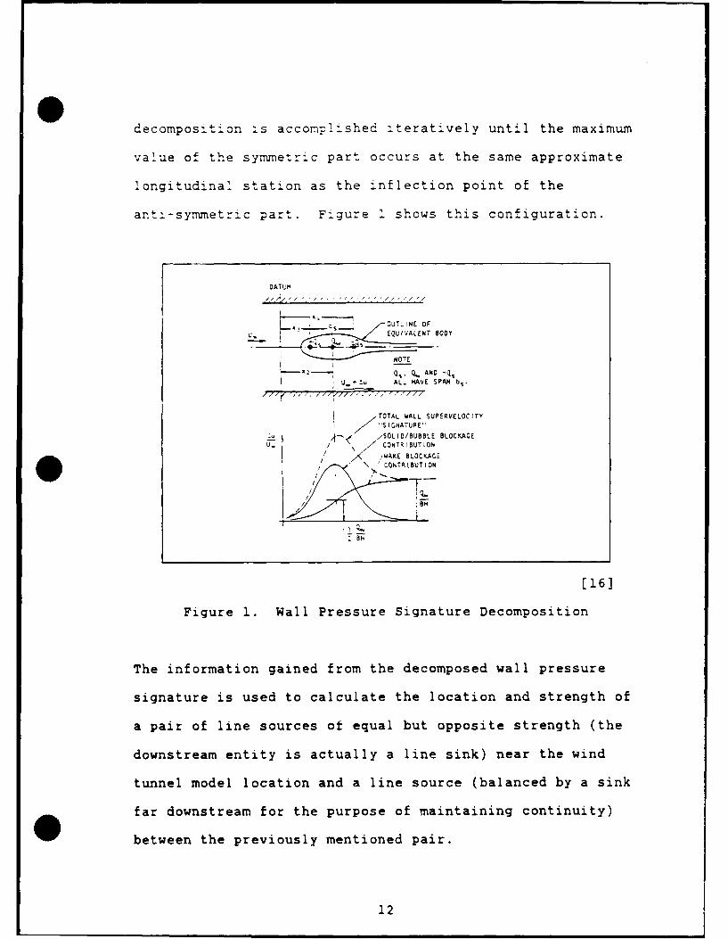
decomposition is accomplished iteratively until the maximum

value of the symmetric part occurs at the same approximate

longitudinal station as the inflection point of the

anti-symmetric part. Figure 1 shows this configuration.

DATUM

- : F OuTL INE OFU_4

sEQUIAL ENT BODY

NOTE.

Q . O ANO -Q,

; U. -2u ALL RAVE SPAN bs .

TOTAL WALL SUPERVELOCITv"S IIGNATURE"/ ' SOLID/BUBBLE BLOCKAGE

U. i < I CONTRIBUTION

/< .,WAKE BLOCKAGE

/ CONTRI BUTION

[16]

Figure 1. Wall Pressure Signature Decomposition

The information gained from the decomposed wall pressure

signature is used to calculate the location and strength of

a pair of line sources of equal but opposite strength (the

downstream entity is actually a line sink) near the wind

tunnel model location and a line source (balanced by a sink

far downstream for the purpose of maintaining continuity)

* between the previously mentioned pair.

12

E

[13]

Figure 2. Location of Line Sources and Sinks

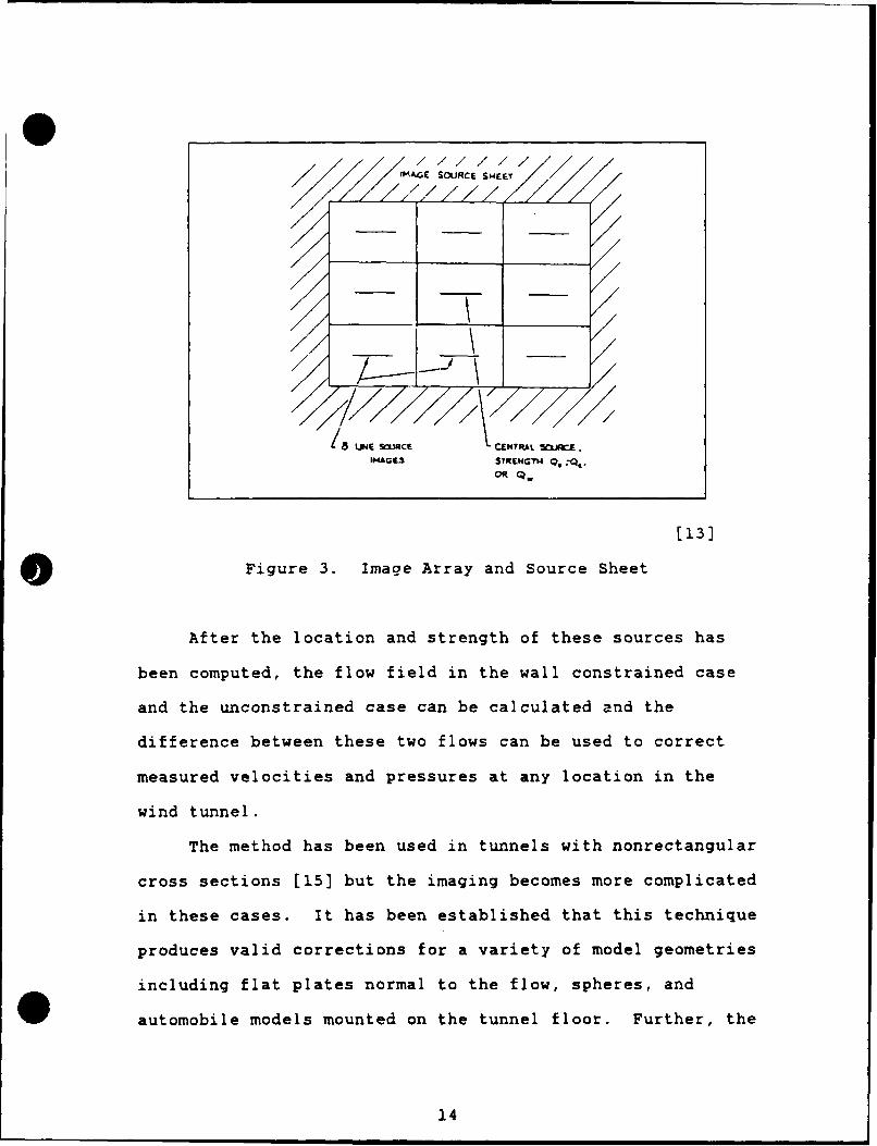
A two dimensional array of images is used to represent

the tunnel walls in the case of a rectangular tunnel. The

array of images is not doubly infinite but instead extends

outwards from the tunnel in a plane perpendicular to the

tunnel axis for only a few images then a source panel is

used to represent the rest of the images as in Figure 3.

This source panel contribution is much faster to compute and

introduces only a small error.

13

///,,/ / / /-/////IAESOURCE SHEE1AGE E ZX

/

/8 LIE souce CENTRAL SC)-.

[13]

Figure 3. Image Array and Source Sheet

After the location and strength of these sources has

been computed, the flow field in the wall constrained case

and the unconstrained case can be calculated and the

difference between these two flows can be used to correct

measured velocities and pressures at any location in the

wind tunnel.

The method has been used in tunnels with nonrectangular

cross sections [153 but the imaging becomes more complicated

in these cases. It has been established that this technique

produces valid corrections for a variety of model geometries

including flat plates normal to the flow, spheres, and

automobile models mounted on the tunnel floor. Further, the

14

corrections seem to allow for useful data to be taken at

larger tunnel cross section blockage ratios than other

correction methods, up to 13.7% in the case of sphere

models. Hackett obtained consistent results from tests

performed in different sized wind tunnels and with a variety

of model sizes in each tunnel. The method was also verified

by Walker and Wiseman [36] for a flat plate mounted normal

to the flow where it was found that various plate sizes

could be corrected to produce essentially the same drag

coefficient. Rae and Pope explain Hackett's method in some

detail under the subject of wind tunnel blockage corrections

[29:chap6]. Hackett implemented the method using look-up

* charts as it proved to be too slow to implement on-line in

the tunnel with the available computers.

Further development, resulting in another method

[12] applicable to winged vehicles, solved the slow computer

limitation. In Hackett's second method, the tunnel walls

are again modeled by imaging, but the solid and wake

blockage are modeled by a single row of vortex panels

centered in the wind tunnel. The geometry of the vortex

panels is assumed and the strengths left as the unknowns.

Since there are more data points (the wall pressure

measurements) than unknowns (vortex strengths), the solution

can be calculated without iteration by a least squares

matrix technique. This produces a correction system that

* can be used on-line in the testing environment.

15

Ashill has used a boundary integral formulation to

calculate the wall induced velocities and upwash at fighter

aircraft, automobile, and flat plate models in a wind tunnel

[1,3]. Results more accurate than those obtained by Maskell

were reported and were accomplished using only about 80 wall

pressure measurement locations on all walls in the wind

tunnel. Zhou has also reported accurate corrections on an

airfoil model using essentially the same formulation as

Ashill [36]. Basically, the method involves calculating the

perturbation potential function due to the tunnel walls and

model.

u - UOx

Where P is velocity potential,

u is perturbation potential,

U is free stream velocity, and

x is in the direction of free stream velocity.

The wall pressure data is used to gain accurate knowledge of

the perturbation potential. Another perturbation potential

may be calculated for the flow about the model in the same

free stream flow but without the tunnel walls included. The

difference between the two perturbation potentials is that

due to the presence of the tunnel walls. The integral

equations used in this method are amenable to Boundary

Element Method (BEM) solution.

16

Again, although almost all of the literature reviewed

referred to wind tunnel experiments, the recent emphasis on

development of wall pressure signature techniques seems to

point to a measurement technique which could be accomplished

in a water tunnel with less complication than other wind

tunnel force and pressure measurement methods. Also, most

of the previous applicable research was aimed at calculating

tunnel corrections to the desired free stream flow

condition, but the desired eventual result from this

research is to measure forces on a model in a flow without

instrumenting the model, but instead by instrumenting the

water tunnel.

17

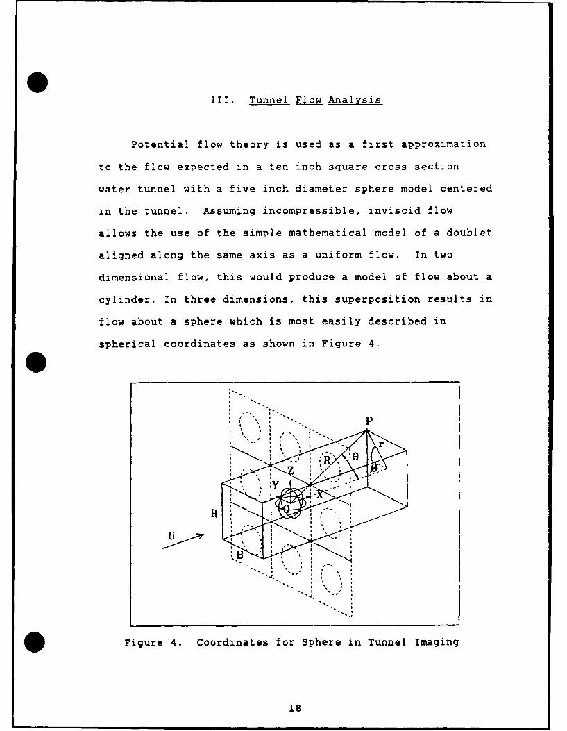
III. Tunnel Flow Analysis

Potential flow theory is used as a first approximation

to the flow expected in a ten inch square cross section

water tunnel with a five inch diameter sphere model centered

in the tunnel. Assuming incompressible, inviscid flow

allows the use of the simple mathematical model of a doublet

aligned along the same axis as a uniform flow. In two

dimensional flow, this would produce a model of flow about a

cylinder. In three dimensions, this superposition results in

flow about a sphere which is most easily described in

spherical coordinates as shown in Figure 4.

Ur: ' , - , I

0.

Figure 4. Coordinates for Sphere in Tunnel Imaging

18

Ignoring, for the moment, the tunnel walls and the

array of doublet images in the YZ plane which are also shown

in the figure above, the velocity potential in spherical

coordinates is given by [21]

P cose(R,,4 ) = UR cos O +

where 4 = velocity potential

R = distance from global origin to point

0,0 = angles defined in figure above

U = free stream velocity

p = doublet strength

The velocity at any point outside of the sphere is [21]

uR = U cosea3R [U 2n R

u= - - U + sinOR ae 4n R

R sine a(

19

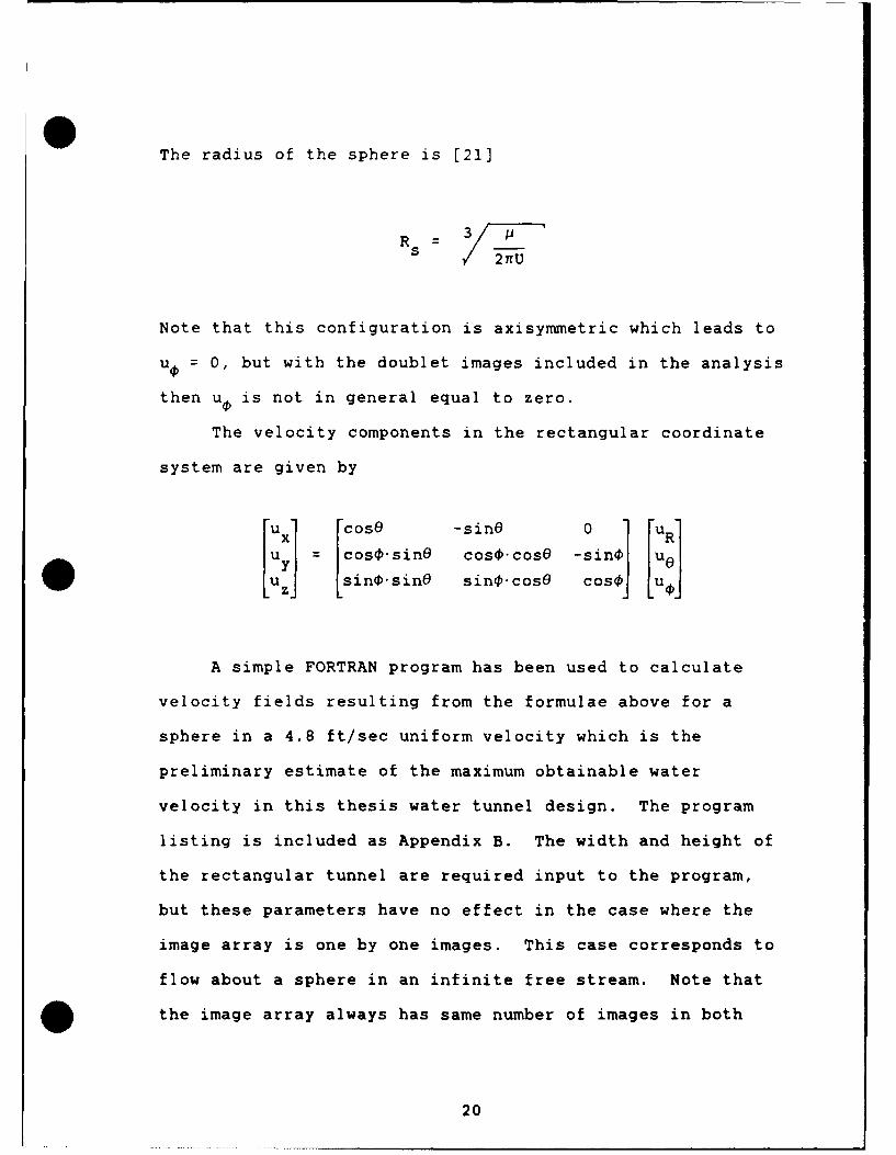
The radius of the sphere is [21]

Rs

Note that this configuration is axisymmetric which leads to

u0 = 0, but with the doublet images included in the analysis

then uP is not in general equal to zero.

The velocity components in the rectangular coordinate

system are given by

[u] [cose -sine 0 ] uRluI c os0.sin0 cosO.cos0 -sinI ueu Z s in.sinO sinOPcose cos4o [u0J

A simple FORTRAN program has been used to calculate

velocity fields resulting from the formulae above for a

sphere in a 4.8 ft/sec uniform velocity which is the

preliminary estimate of the maximum obtainable water

velocity in this thesis water tunnel design. The program

listing is included as Appendix B. The width and height of

the rectangular tunnel are required input to the program,

but these parameters have no effect in the case where the

image array is one by one images. This case corresponds to

flow about a sphere in an infinite free stream. Note that

*the image array always has same number of images in both

20

directions in the YZ plane and that the array dimernsion

should be an odd number so the central image is the domain

of interest.

As the image array size is increased, the flow fields

calculated more resemble flow in a tunnel in that the

velocity at a wall location (actually the mid point between

the central image and the next nearest image) has lesser

components in the Y or Z direction, whichever direction is

the normal to the particular wall in question. Larger image

array sizes also slow the computations considerably,

especially when generating a velocity field at many points.

An array size of 21 was deemed optimal since a desk top

computer generated results fairly quickly with this value

and the numerical error occurred only after three

significant digits when compared to results generated with a

1,000 by 1,000 array of images. The computations with such

large arrays took an impracticably long time to accomplish

and clearly indicated that the effects of image doublets at

the large distances involved are negligible. This was

expected as the velocity components contain R3 terms in the

denominator. These numerical errors are even less important

when considered along with the error introduced with the

original assumption of inviscid flow in this analysis. The

fact that this potential flow analysis predicts no wake

blockage at all is its most serious shortcoming.

Nevertheless, the flow parameters predicted on the tunnel

21

walls ox the upstream side of the sphere are expected to be

accurate enough to make design decisions for preliminary

instrumntation for the water tunnel and for the tunnel test

sectiom design itself.

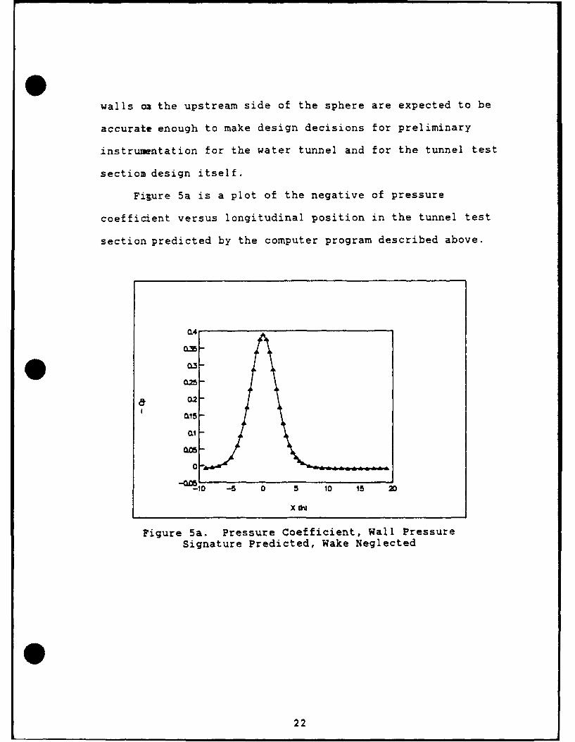
Filure 5a is a plot of the negative of pressure

coefficient versus longitudinal position in the tunnel test

section predicted by the computer program described above.

ioA& 024

0.3-

025-

0-

-0 -5 0 5 10 15 20

Figure 5a. Pressure Coefficient, Wall PressureSignature Predicted, Wake Neglected

22

The usual definition of pressure coefficient as

cp = 1 - [;12

~u

where u = local velocity

U = free stream velocity

is used in this analysis. The markers on the plot indicate

the locations of static pressure ports along the centerline

of the test section windows. The overall shape of the plot

is the same as the shape of the symmetric part of the plot

in Figure 1. Recall that the anti-symmetric part of a wall

pressure signature is that attributed to wake blockage. The

magnitude of the predicted wall pressure signature is on the

same order as some of those reported by Hackett [16] for a

sphere model which spans half of the height of a 30" by 43"

wind tunnel, in subcritical flow with a Reynold's number

about 220,000.

The previous analysis can be improved by the addition

of the velocity contribution to the flow of a Rankine oval

to simulate the wake blockage effect. This is done by

placing a point source on the downstream x-axis at its

intersection with the model sphere surface. A point sink is

placed on the positive x-axis far downstream. The velocity

potential for a point source at the origin is [21]

q0(r = =~-

47 r

which leads to the velocity components induced by the source

23

at any other point given in cartesian coordinates as [21]

q xU x(XYZ) =- ( 2 + z2)3/2

q yU x(XYZ) - 2 2 2)3/2

41 x 2 + y+ z

q zU X(XY'Z) =- 2 y2 2)3/4z (x + y + z2J3/2

where q = source strength (negative value for a sink)

The FORTRAN program in Appendix B includes the effect of

sources and sinks of any specified strength placed along the

x-axis which should be interpreted as the centerline of a

rectangular tunnel. In this analysis, however, only a

source on the downstream side of the sphere model and a sink

far downstream are used.

The resulting wall pressure signature from a doublet, a

Rankine oval as just described, and a uniform flow is shown

in Figure 5b. The source and sink strength are taken as

equal to the doublet strength which in this particular case

produces a wake diameter consistent with flow separation

from a five ir'-h sphere at approximately 1400 from the

upstream stagnation point. Note that the effect of adding

this Rankine oval has produced little effect on the wall

pressure signature upstream of the doublet (the sphere

24

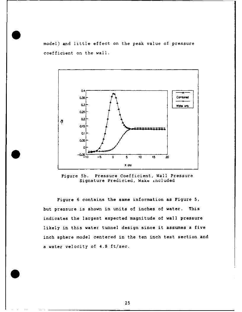
model) and little effect on the peak value of pressure

coefficient on the wall.

O4

WCe Coy

025-

2 -

01-

O0

0

-10 -5 0 5 10 15

X OV~

Figure 5b. Pressure Coefficient, Wall PressureSignature Predicted, Wake included

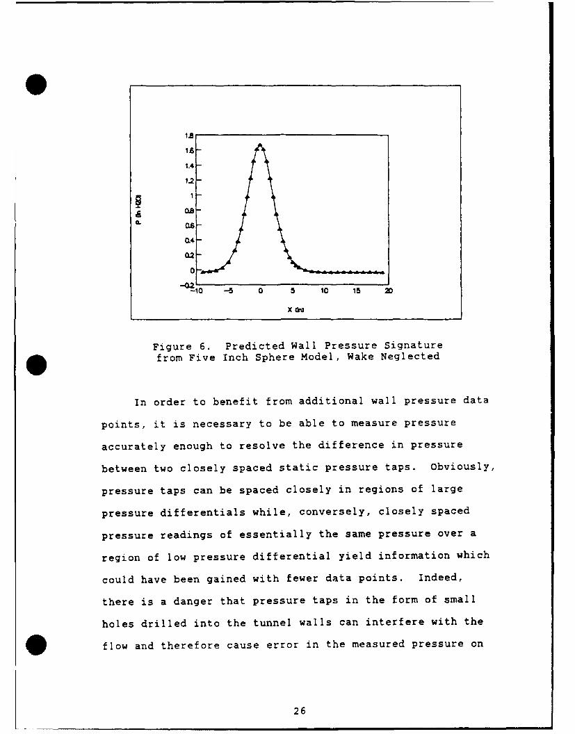
Figure 6 contains the same information as Figure 5,

but pressure is shown in units of inches of water. This

indicates the largest expected magnitude of wall pressure

likely in this water tunnel design since it assumes a five

inch sphere model centered in the ten inch test section and

a water velocity of 4.8 ft/sec.

25

1.4

1.2-

04

02

0

-10il -5 0 5 10 15 2D

x ft

Figure 6. Predicted Wall Pressure Signaturefrom Five Inch Sphere Model, Wake Neglected

In order to benefit from additional wall pressure data

points, it is necessary to be able to measure pressure

accurately enough to resolve the difference in pressure

between two closely spaced static pressure taps. Obviously,

pressure taps can be spaced closely in regions of large

pressure differentials while, conversely, closely spaced

pressure readings of essentially the same pressure over a

region of low pressure differential yield information which

could have been gained with fewer data points. Indeed,

there is a danger that pressure taps in the form of small

holes drilled into the tunnel walls can interfere with the

flow and therefore cause error in the measured pressure on

26

other pressure taps further downstream. This risk increases

with additional closely spaced pressure taps.

Figure 7a shows the expected difference in pressure

between adjacent static pressure ports for the previously

described example of a half tunnel span sphere model.

0.3

02-

QLI

0CL

-a2

5-10 - 0 5 10 15

X a

Figure 7a. Pressure Differences Along WindowCenterline, Wake Neglected

For this figure, the pressure ports are located along the

centerline of a tunnel wall and spaced one inch apart except

for a region near the sphere model where the spacing is

one-half inch. One pair of acrylic test section windows has

been modified to this configuration. The small

discontinuities in the otherwise smooth curve in Figure 7

* are due to the transition point from one inch port spacing

27

to one-half inch port spacing. Note that this is not a plot

of ap/Ox versus x which would be a smooth curve throughout

but is a plot of pressure differences calculated from point

to point with some variation in the point spacing. The

conclusion drawn from this figure is that pressure

differences must be measured to an accuracy of 0.001

inches of water which is one order of magnitude smaller than

the smallest pressure difference predicted near the sphere

model location to accurately represent a wall pressure

signature similar in magnitude to that shown in Figure 6.

The need for accuracy in pressure measurement increases

with smaller models and with lower flow velocities.

Figure 7b shows the same information as Figure 7a

except that the effect of the wake simulated by a Rankine

oval is included. The pressure differences shown on the

upstream portions of both curves are essentially the same

while the downstream portion of Figure 7b shows a smaller

peak pressure difference. Including the wake effect in the

analysis does not substantially change the accuracy required

of the wall pressure signature measuring instruments.

28

OO

0.1

0

-412

-. 3-10 -5 0 5 10 15

x

Figure 7b. Pressure Differences Along WindowCenterline, Wake Included

All of the preceding analysis concerned pressure

measurements taken along the centerline in the flow

direction of a test section wall or window. As shown in

Figure 8a which is a contour plot of the negative of

pressure coefficient over an entire test section window,

this is exactly where the largest pressure gradients are

located.

29

-9.00 -6.54 -4.09 -1.63 0.82 3.28 5.74 8.19 10.65 13.11 15.56 18.025.00 - 5.00

2 50 2 50

0 O0 0 o

000 000

-2 50 / -2 50

-5 00 -500-900 -654 -409 -1.63 0.82 3.28 5.74 819 10.65 13 11 1556 1802

Figure 8a. Pressure Coefficient on Test Section Wall,Wake Neglected

It is also apparent from Figure 8a that not much variation

of pressure exists perpendicular to the flow direction on

the wall except at x = 0. If it were desired to add more

pressure ports to the existing array along the window

centerline it seems that the most useful configuration would

be ports spaced along a single line perpendicular to the

flow and centered on the model location. The total array of

ports would then form a cross centered on the model. Figure

8b shows that this same configuration is indicated even when

wake effects are included in the analysis. The most

important difference between Figure 8a and Figure 8b is that

the pressure coefficient downstream of the model location is

larger in Figure 8b while the contours in Figure 8a are

symmetric about the sphere location at x=O.

30

-g.oo -6.50 -400 -1.50 1.00 3.50 6.00 8.50 11.00 13.50 16.00 18.505.00 = 5.00

3.00 3.00

1.00 1.00

- 1.00 -1.00

-3.00 /-3.00

-5.00 -5.00-9.00 -6.50 -4.00 -1.50 1.00 3.50 5.o a.50 11.00 13.50 15.00 18.50

Figure 8b. Pressure Coefficient on TestSection Wall, Wake Included

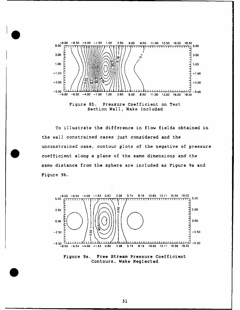
To illustrate the difference in flow fields obtained in

the wall constrained cases just considered and the

unconstrained case, contour plots of the negative of pressure

coefficient along a plane of the same dimensions and the

same distance from the sphere are included as Figure 9a and

Figure 9b.

-9.00 -6.54 -4.09 -1.63 0.82 3.28 5.74 8.19 10.65 13.11 15.56 15.025.00 5.00

2.50 2.50

0.00 0.00

-2 50 o-2.50-0

Contours, Wake Neglected

31

-9.00 -05.50 -4.00 -1.50 1.00 5.50 5.00 8.50 11.00 123.50 18.00 18.501.00 r1.00

-1.O -1.00

-3.00 -3.00

-5.00 -5.00-9.00 -6.50 -4.00 -1.50 1.00 3.50 8.00 8.50 11.00 13.50 16.00 18.50

Figure 9b. Free Stream Pressure CoefficientContours, Wake Included

For this unconstrained flow case, the overall pressure

coefficient and the pressure gradients are smaller. Also

the region where the pressure coefficient changes sign

(which indicates flow velocity lower than free stream

velocity in this case) is closer to the model location. The

maximum pressure gradient is still along a line in the

direction of the flow.

Note that Figures 8b and 9b contain the information

necessary to calculate tunnel corrections to unconstrained

stream values for the given model. Suppose that

experimental data corresponding to the case predicted in

Figure 8b was available and that it was desired to correct

this data to calculate the pressure expected in an

unconstrained flow. Then it would be necessary to take the

difference in the velocity fields corresponding to Figures

8b and 9b, and add this difference to the velocity

32

field measured in the experiment. The technique just

described does not consider the effects of boundary layer

growth along tunnel walls, or the effects of tunnel wall

confinement on wake and vortex trajectories.

The result of this flow analysis is that the geometry

of the test section design is shown to be likely to yield

measurable wall pressure signatures with a simple spherical

model centered in the tunnel. The analysis also predicts

the nature of the experimental data to be taken in the

preliminary research conducted in this water tunnel assuming

that close to uniform flow is achieved with this tunnel

design.

33

IV. DESIGN OF WATER TUNNEL

Primary Requirements

The primary performance requirements for a water tunnel

test section for this study are that uniform flow be

provided at a high enough velocity so that wall pressure

signatures can be measured conveniently. It is also

desirable to change as little as possible the existing test

rig in test cell 23 on the first floor of building 18 since

the experiment now in place will continue to be useful for

some time.

Description of Present Facility_

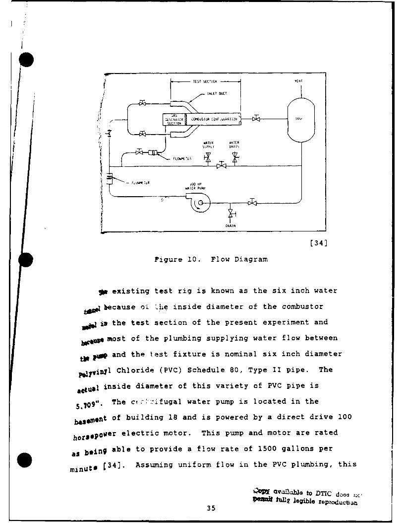
The experiment presently installed in the water tunnel

is the Multi-Ducted Inlet Combustor [34]. A block diagram

of the water flow used in this experiment is included in

Figure 10.

34

(TEST SECTION WE N T

WER WATER

RLAIER PUM

[34)

Figure 10. Flow Diagram

*v existing test rig is known as the six inch water

tdibecause ol. '.he inside diameter of the combustor

as* is the test section of the present experiment and

,,,wtmost of the plumbing supplying water flow between

tior~vand the test fixture is nominal six inch diameter

,VnlChloride (PVC) Schedule 80, Type II pipe. The

actual inside diameter of this variety of PVC pipe is

5.09 of The cfc.<:ifugal water pump is located in the

baseentof building 18 and is powered by a direct drive 100

hors power electric motor. This pump and motor are rated

as being able to provide a flow rate of 1500 gallons per

minuts [34]. Assuming uniform flow in the PVC plumbing, this

Sal"'31dj1 to DTIC dones;c

35 fullf legible reproductian

corresponds to a water velocity of 18.8 feet per second.

Using this velocity and taking the water temperature as

60 0F, which is the lowest temperature the tunnel is likely

to experience, a Reynolds number of 733,000 is obtained

based on the pipe diameter. Obviously, this is much greater

than Reynolds upper critical number of 4,000 for usual

piping installations [35] and fully developed turbulent flow

is expected in the PVC plumbing at all times.

The water supply is routed through a water softener

located next to the pump and motor, and valves are provided

to either manually fill the test rig quickly or

automatically maintain a desired water level. It is

sometimes desired to leave the tunnel drain slightly open

and have the water supply automatically maintain the level

with fresh water since this keeps the water temperature

lower than it would be otherwise. Continuous operation of

the tunnel can easily cause the water temperature to rise to

1200 F or more. The PVC and Acrylic construction of most of

the test rig could withstand somewhat higher temperatures,

150 F or more, and operator safety is not much of a concern

at this temperature, but the increase in vapor pressure of

water with temperature will cause cavitation in low pressure

regions of the test section flow.

In the test cell, the PVC plumbing providing water

flow from the pump is supported within an adjustable steel

rack which is 20 feet long, 2.5 feet wide and about three

36

feet high. The test section and instrumentation is mounted

on tcp of thiS rack at alout fi%-e feet above flcor level.

Immediately downstream of the experiment is a large steel

settling chamber about five feet in diameter and six feet

high. The settling chamber receives all water flow from the

experiment before routing the water back to the pump. This

chamber also has a six inch diameter stack extending from

the top which is kept nearly full during tunnel operation

for the purpose of maintaining a high water pressure in the

test section. With the stack full, the static pressure in

the test section is about 60" of water or 2.2 psig

depending on the exact height at the location in question in

the test section.

Modifications to Present Facility

Installation of the 10 inch square test section

requires that the present test section be disassembled and

removed. The existing supporting rack remains necessary, but

many of the adjustable support brackets need to be moved and

new brackets built. An extension to the support rack is

needed as the new test rig is about seven feet longer than

the present one. The PVC water supply pipe must also be

extended about seven feet at the upstream end of the test

section. At the downstream end of the test section, the

stagnation tank requires no modification. No modification

* of the water flow controls are envisioned at this time other

37

than moving the six inch butterfly shutoff valve at the

upstream end of the test section to accommodate the

extension in length. It must be possible to reinstall the

Multi-Ducted Inlet Combustor model with minimal

modifications to the existing interface fixtures related to

the extension in length of the support rack.

Design of Ten Inch Square Water Tunnel

As previously mentioned, the primary requirements for

this water tunnel are that uniform flow be provided at a

high encgh velocity to be able to conveniently measure

pressure differences due to solid and wake blockage at

0closely spaced stations along the tunnel walls. This

velocity is required to provide a Reynolds number comparable

to those obtained in the Air Force Institute of Technology

(AFIT) 14" low speed wind tunnel. These considerations lead

to the smallest possible test cross sectional area.

Opposing this consideration is a secondary requirement that

models of a convenient size, and possibly the identical

models used in other AFIT test facilities such as the

planned 14" square wind tunnel in Building 95, fit in this

water tunnel.

Test Section. A 10" square test section was chosen

which will provide a water flow velocity of 4.81 feet per

second assuming uniform flow. Preliminary calculations

indicate that a Reynolds number range of 329,000 to 658,000

38

may be obtained by controlling the water temperature from

0 0,60 F Lo 120 . These figures assume that the full 1,500

gallons per minute flow rate is achievable, and the

characteristic length is taken to be the test width of ten

inches. A technique currently used in the facility for

temperature control consists of running the tunnel at high

speed to raise the temperature from internal friction, and

draining water from the tunnel while replenishing with cold

tap water to lower the temperature. The increased

occurrence of cavitation at higher temperatures is

unfortunate because it will often be desired to run

experiments at the highest possible Reynolds number. The

* decrease in viscosity with higher temperature will both

directly raise the Reynolds number and may decrease pipe

friction loses which will allow greater velocity also

raising the Reynolds number. The technique of running water

tunnels at elevated temperatures to produce a high Reynold's

number is well known and a description of its use is given

by Stahl [33]. This range of Reynolds number, assuming an

air temperature of 590F and based on a characteristic length

of 14", would be achieved in the AFIT low-speed wind tunnel

at velocities of 44.1 to 88.3 feet per second.

The test section is constructed mainly of 0.62"

thick aluminum, bolted together with 10-24 socket head

screws and sealed with 0.100" nominal linear O-ring

cord. See Figures 18-32 in Appendix A for drawings. The

39

side walls are acrylic windows which are also bolted in

place and sealed with O-ring cord. See figures 33-37.

Three pairs of windows have been machined with two sets left

unmodified for future use and one set drilled for static

pressure taps spaced every one inch down the centerline of

the length of the window. The pressure tap spacing is

one-half inch in the vicinity of the proposed model location

which is 10" downstream from the beginning of the

window. This pressure tap spacing scheme was selected based

on the expected wall pressure signature from a spherical

rrodel, discussed in the previous section of this thesis,

which spans one-half of the test section for a cross

sectional area blockage ratio of 19.6%. Although the

pressure on the windows is only predicted to be between 2.5

to 3.5 psi above atmospheric, this integrates to about 900

pound. force and there was some concern about the ability of

the window flange to withstand the load. See Appendix C for

a structural analysis which concludes that the design has

sufficient strength.

A Pitot tube rake extending the full height of the

tunnel (see Figure 38 and 39, Appendix A) is mounted in the

tunnel with the fifteen total head probes arrayed

vertically. The rake is attached to the tunnel by 0.25"

diameter stainless steel rods passing through compression

fittings installed in the windows. These compression

fittings have had the normal stainless steel ferrules

40

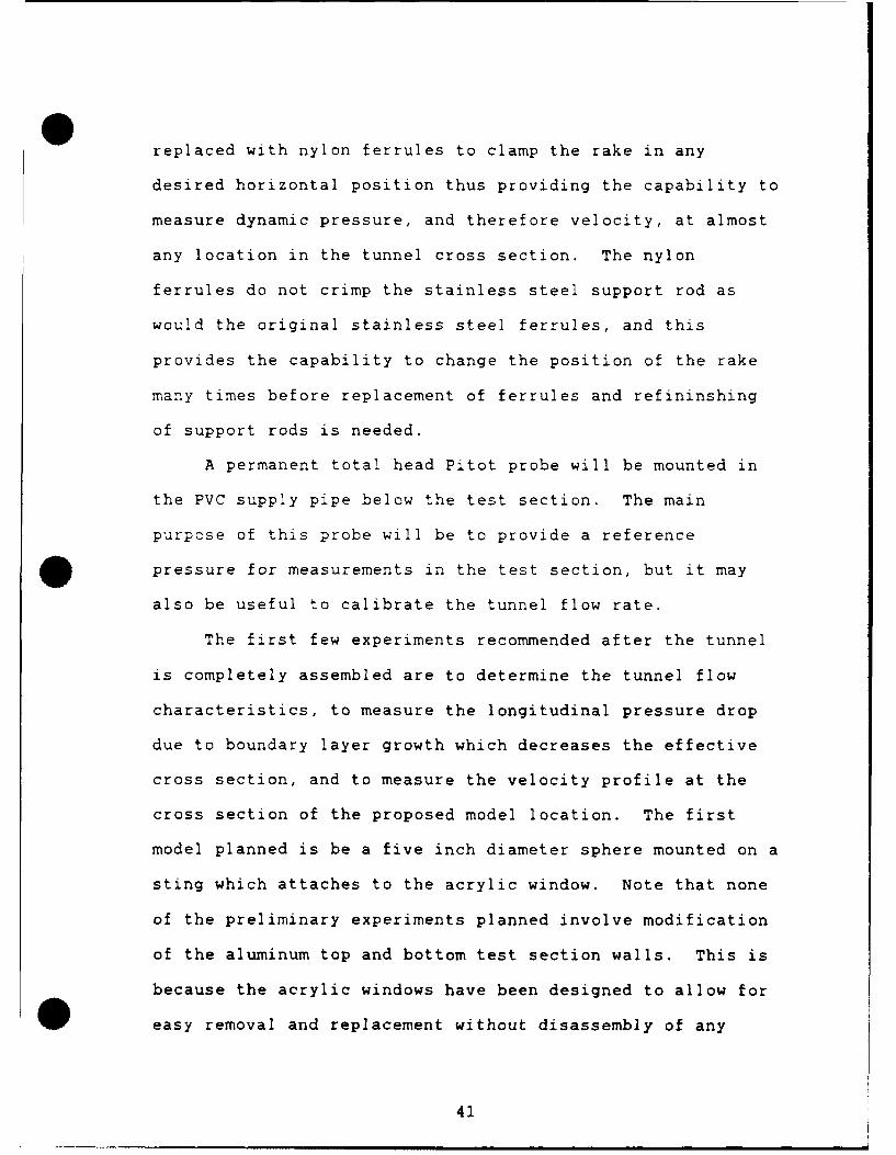
replaced with nylon ferrules to clamp the rake in any

desired horizontal position thus providing the capability to

measure dynamic pressure, and therefore velocity, at almost

any location in the tunnel cross section. The nylon

ferrules do not crimp the stainless steel support rod as

would the original stainless steel ferrules, and this

provides the capability to change the position of the rake

many times before replacement of ferrules and refininshing

of support rods is needed.

A permanent total head Pitot probe will be mounted in

the PVC supply pipe below the test section. The main

purpcse of this probe will be to provide a reference

0pressure for measurements in the test section, but it may

also be useful to calibrate the tunnel flow rate.

The first few experiments recommended after the tunnel

is completely assembled are to determine the tunnel flow

characteristics, to measure the longitudinal pressure drop

due to boundary layer growth which decreases the effective

cross section, and to measure the velocity profile at the

cross section of the proposed model location. The first

model planned is be a five inch diameter sphere mounted on a

sting which attaches to the acrylic window. Note that none

of the preliminary experiments planned involve modification

of the aluminum top and bottom test section walls. This is

because the acrylic windows have been designed to allow for

easy removal and replacement without disassembly of any

41

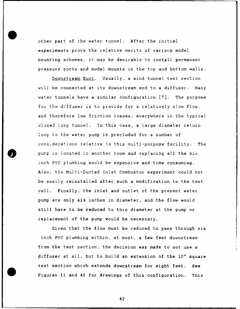
other part of the water tunnel. After the initial

experiments prove the relative merits of variotus model

mounting schemes, it may be desirable to install permanent

pressure ports and model mounts in the top and bottom walls.

Downstream Duct. Usually, a wind tunnel test section

will be connected at its downstream end to a diffuser. Many

water tunnels have a similar configuration [7]. The purpose

for the diffuser is to provide for a relatively slow flow,

and therefore low friction losses, everywhere in the typical

closed loop tunnel. In this case, a large diameter return

loop to the water pump is precluded for a number of

considerations relative to this multi-purpose facility. The

pump is located in another room and replacing all the six

inch PVC plumbing would be expensive and time consuming.

Also, the Multi-Ducted Inlet Combustor experiment could not

be easily reinstalled after such a modification to the test

cell. Finally, the inlet and outlet of the present water

pump are only six inches in diameter, and the flow would

still have to be reduced to this diameter at the pump or

replacement of the pump would be necessary.

Given that the flow must be reduced to pass through six

inch PVC plumbing within, at most, a few feet downstream

from the test section, the decision was made to not use a

diffuser at all, but to build an extension of the 10" square

test section which extends downstream for eight feet. See

Figures 11 and 40 for drawings of this configuration. This

42

length was selected as the largest that could be

accommodated in the test cell and also as the largest

commonly available dimension of 0.75" thick acrylic sheet of

which this duct was constructed. This acrylic construction

could be a benefit as the flow in the tunnel can be directly

viewed over a much longer than typical test length.

An adapter was designed to attach this duct to the PVC

plumbing without much concern for the flow characteristics

in the adapter. The most likely form of a disturbance in

the test section due to this adapter would be from vortices

generated near the corners of the adapter interface with the

square duct and the strength of the induced velocities would

be inversely proportional to distance from the vortices

[21]. The adapter is eight feet downstream from the test

section; therefore, flow in the test section is not

expected to be affected to a measurable degree. See figures

40-47 in Appendix A for drawings.

Upstream Diffuser and Stilling Tank. The purpose of

these components is to bring the water flow to as low a

velocity as possible immediately before it passes into the

test section. Any flow conditioning devices, such as

screens to reduce axial velocity differences at a cross

section or honeycombs to remove large scale turbulence, will

cause less frictional losses when implemented in a

relatively slow flow [29:chap 2]. The major design

*consideration for this diffuser is avoidance of separation

43

since a separated flow produces a jet of high velocity

water in the center of the diffuser, stilling tank and

nozzle which makes it impossible to have uniform flow in

the test section.

The geometry of the diffuser is a straight cone

with a semi-vertex angle of 70 which was selected for

reasons of both flow performance and ease of fabrication.

KlIne [22:309] shows that this is about the largest angle at

which no stall will occur over a Reynold's number range of

6,0CD to 300,000 for flat plane-walled diffusers operating

in water. Interestingly, in further research [23] extending

this work to other geometries including straight cone

diffusers, the same 70 semi-vertex angle was shown to be

close to the optimal angle for pressure recovery indicating

the least possible frictional losses. Gibson [8] compared

several diffuser geometries including square, rectangular,

and round cross section and straight versus curved diverging

boundaries and found that straight cone circular cross

section diffusers of about this semi-vertex angle produced

the lowest losses of the diffusers tested. Gibson's results

also suggest that any performance benefit in a more

complicated diffuser design would be small. A more

complicated design would probably be longer than the

straight cone design to produce the same overall area ratio

since the maximum slope in the diffuser is always limited by

the same avoidance of separation consideration. The

44

conclusion is that a more complicated diffuser design

would yield little, if any, flow performance benefit and the

additional complications involved in design and construction

are unwarranted [24].

The area ratio achievable in this design is limited by

the available length in the test cell. To produce a 24"

inside diameter in the stilling tank with the previously

mentioned 70 semi-vertex angle, the diffuser m'ist be 73.3"

long. This gives an area ratio of 4.2 and a

predicted velocity in the stilling tank of 1.14 feet per

second. This velocity assumes uniform flow and a pump flow

rate of 1,500 gallons per minute. See Figures 12-16 in

* Appendix A for drawings.

Nozzle. The purpose of the nozzle is to accelerate the

flow to the high velocity needed in the test section in a

manner producing as uniform a flow as possible. Separated

flow is not so much a concern for the nozzle as it is for

the diffuser because the pressure gradient in the flow

direction will be negative throughout a properly designed

nozzle. A complication arises, however, from the fact that

the entrance to the nozzle will be circular in cross section

while the exit will be square. See Figure 17 in Appendix A

for drawings. A description of the nozzle geometry is given

in Appendix D.

Instrumentation. To measure wall pressure signatures,

* it is necessary to measure the static pressure at a large

45

numd ports on the tunnel walls. The pair of test

se~mwindows to be used first have static pressure ports

spaevery one inch down the centerline starting at one

incWd ending at 29 inches (29 ports) and every one-half

incI the vicinity of the model from 6.5 inches to 15.5

incb 1 0 additional ports). The reference pressure for

the ,asurements will be either the pressure at the

furt, upstream static pressure port or the total pressure

:nt . t~aater supply pipe below the test section since a

tota:gessure probe will already be mounted there to serve

as a.4erence value in measuring velocity profiles in the

test Wtion With an axi-symmetric model, it may only be

necesWY to take measurements along one wall; however,

measlzeents along at least two walls will be needed for a

Iifti2 model. Thus the possibility arises that 78 static

pressure measurements must be made over a short period of

time. sd quite possibly more measurements than this for

experiments that involve unsteady flow, asymmetric model

geometrY, or asymmetric model location.

No supplier of a scani-valve suitable for use in water

was found and it is doubtful that such a device exists. One

reason this is a problem is that pressure transducers

capable of resolving the small pressure differences

predicted between adjacent static ports in this tunnel

design are very expensive, on the order of $1,000 or more

each for variable reluctance pressure transducers suitable

46tV:Ne to DTTc

46

for use in water. Without a scani-valve a large number of

transducers will be needed to take simultaneous measurements

and at this stage of development the risk of selecting an

inapprcpriate transducer precludes such a large expenditure.

it may be possible to use a transducer which is limited

tc pressure measurements in gases by designing a trap to

keep the transducer input from coming in contact with the

water. For example, the transducer can be connected to a

pressure port with a long plastic tube which forms a high

loop above the highest water level in the test rig. The

advantage to this is that such transducers are available for

about $150 each. However, such a configuration invites

* damage to the transducers in case of any deviation from the

tunnel operation procedures which would need to be developed

to keep water from siphoning into the transducers. Another

disadvantage of this scheme is that longer tube length will

slow the time response of pressure measurements. Slow

response Is not so important when measuring steady flow

effects, in fact it could help by dampening noise from small

scale turbulence, but a slow responding measurement system

would limit the type of research that can be undertaken in

this facility. Consequently, it was decided to defer the

selection of transducers until after preliminary experiments

have been completed using manometers as instrumentation.

Another transducer to measure wall pressure signatures

* which appears to offer both performance and economic

47

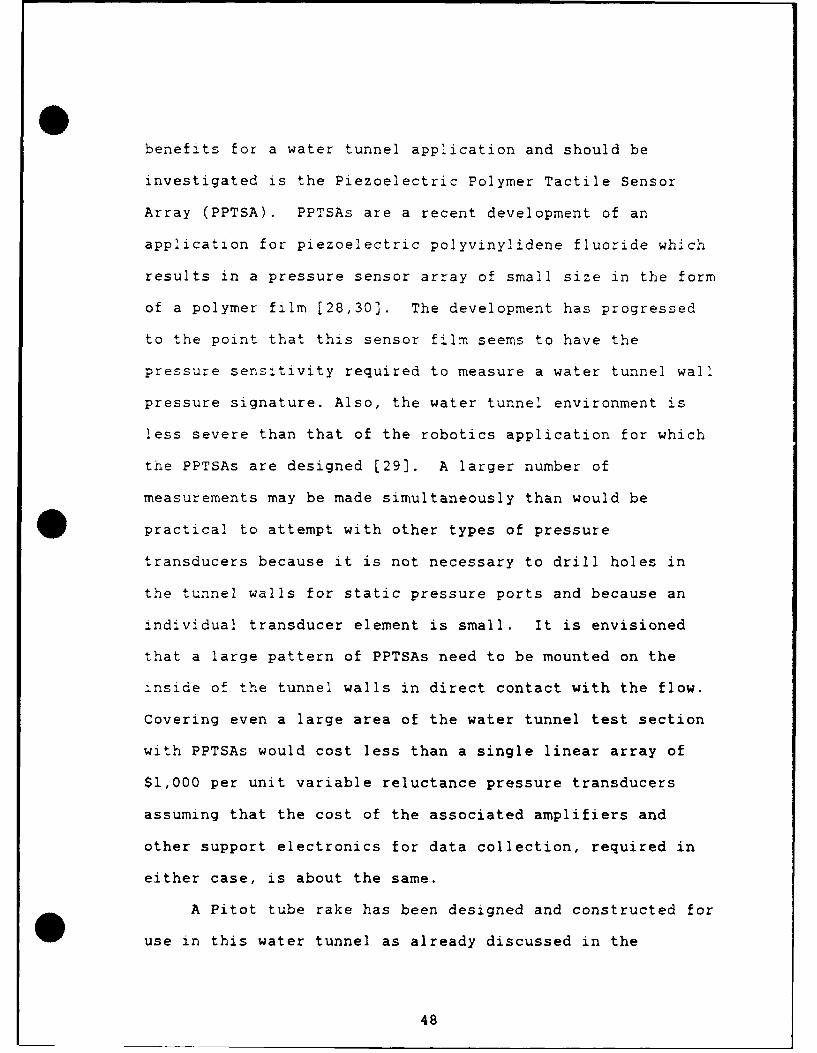
benefits for a water tunnel application and should be

investigated is the Piezoelectric Polymer Tactile Sensor

Array (PPTSA). PPTSAs are a recent development of an

application for piezoelectric polyvinylidene fluoride which

results in a pressure sensor array of small size in the form

of a polymer film [28,30]. The development has progressed

to the point that this sensor film seems to have the

pressure sensitivity required to measure a water tunnel wall

pressure signature. Also, the water tunnel environment is

less severe than that of the robotics application for which

the PPTSAs are designed [29]. A larger number of

measurements may be made simultaneously than would be

practical to attempt with other types of pressure

transducers because it is not necessary to drill holes in

the tunnel walls for static pressure ports and because an

individual transducer element is small. It is envisioned

that a large pattern of PPTSAs need to be mounted on the

inside of the tunnel walls in direct contact with the flow.

Covering even a large area of the water tunnel test section

with PPTSAs would cost less than a single linear array of

$1,000 per unit variable reluctance pressure transducers

assuming that the cost of the associated amplifiers and

other support electronics for data collection, required in

either case, is about the same.

A Pitot tube rake has been designed and constructed for

use in this water tunnel as already discussed in the

48

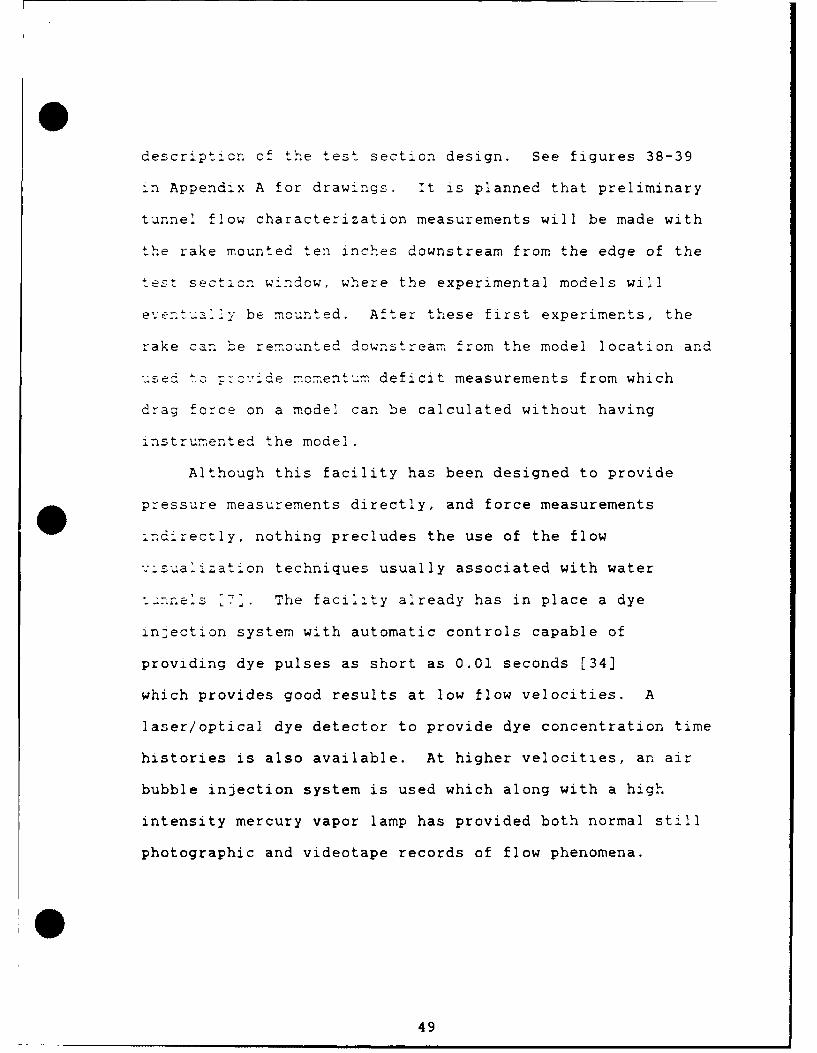
description of the test section design. See figures 38-39

:n Appendix A for drawings. It is planned that preliminary

tunnel flow characterization measurements will be made with

the rake mounted ten inches downstream from the edge of the

test sect2.cn window, where the experimental models will

eventualy be mounted. After these first experiments, the

rake can be remounted downstream from the model location and

used to -:c'.ide momentum deficit measurements from which

drag force on a mode: can be calculated without having

instrumented the model.

Although this facility has been designed to provide

pressure measurements directly, and force measurements

:ndirectly, nothing precludes the use of the flow

v-sualizat-on techniques usually associated with water

- nnes :7'. The facility already has in place a dye

injection system with automatic controls capable of

providing dye pulses as short as 0.01 seconds [34]

which provides good results at low flow velocities. A

laser/optical dye detector to provide dye concentration time

histories is also available. At higher velocities, an air

bubble injection system is used which along with a high

intensity mercury vapor lamp has provided both normal still

photographic and videotape records of flow phenomena.

49

V. Conclusions and Recommendations

The wa'l pressure signature method has been shown to be

feasible as a water tunnel experimental research project by

analysis of the flow around a spherical model in a

rectangular tunnel. The results of this analysis have been

used to make design decisions concerning a new test section

which has been constructed for the Aero Propulsion

Laboratory's six inch water tunnel.

Combined with the boundary element method, wall

pressure signature measurement in the water tunnel should

yield a solution for the flow characteristics at every point

in the flow within the tunnel test section. With the flow

field known, the resultant force on the model in the flow

can be calculated. The pitot tube rake mounted downstream

from the model provides a means of measuring the momentum

deficit in the flow which can be used to calculate the drag

on the model. The pitot tube rake can also be used to

provide input to a boundary element method analysis such as

the velocity profile across the downstream boundary and the size

and location of the viscous wake which defines the shape of

portions of the boundary.

Flow visualization techniques should also be used to

provide input to the boundary element method. The size and

lccation of separation bubbles and wakes due to a model

should be found by injecting dye, or air bubbles as

5o

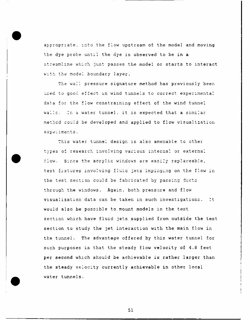
aFppropriate, into the flow upstream of the model and moving

the dye probe until the dye is observed to be in a

streamline which just passes the model or starts to interact

wi.t the model boundary layer.

The wal! pressure signature method has previously been

used to good effect in wind tunnels to correct exper:mental

data for the flow constraining effect of the wind tunnel

wa's,. in a water tunnel, it is expected that a similar

methcd could be developed and applied to flow visualization

expeLlments.

This water tunnel design is also amenable to other

types of research invclving various internal or external

flow. Since the acrylic windcws are easily replaceable,

test fixtures involving fluid jets impinging on the flow in

the test section could be fabricated by passing ducts

through the windows. Again, both pressure and flow

visualization data can be taken in such investigations. it

would also be possible to mount models in the test

section which have fluid jets supplied from outside the test

section to study the jet interaction with the main flow in

the tunnel. The advantage offered by this water tunnel for

such purposes is that the steady flow velocity of 4.8 feet

per second which should be achievable is rather larger than

the steady velocity currently achievable in other local

water tunnels.

51

It is recom ended that the first series of experiments

• "n in the wate tunnel be aimed at characterizing the flow

the test section at all flow velocities up to full speed.

- _~..~ . nc'lude measurement of the wall pressure

.natu:re x no model or pitot tube rake present to

det ::-.> the longitudinal variation of pressure in the test

:e:t zn at various velocities. Next, the pitot tube rake

znu' "D be used to measure velocity profiles at the cross

sec:ion where subsequent research will have models mounted.

t .a a-so be possible to measure velocity profiles with a

zatron tech.ique of injecting dye pulses

simultaneously at various points in the flow and measuring

the dye pulse trajectories over time with either still

photography or a videotape system. These velocity profiles

should be used to decide what, if any, flow conditioning

devices such as screens or honeycombs need to be mounted in

the stilling tank upstream from the test section. This is

an iterative process where the entire series of measurements

should be repeated after each change to the configuration of

the tunnel.

Only after the most uniform possible flow at high

velocity is established should measurements be attempted

with a model. The first model is presently envisioned to be

a five inch diameter sphere mounted on a sting support.

' ThiZ model should have several static pressure taps on its

surface which are connected to instrumentation through the

52

sting support which passes through one of the acrylic

win: ws dow:' L- cf the model.

The previously described fLow characterization

measurements should be repeated with only the sting model

support installed and then again with the sphere model also

insta' led. The data thus collected should be used to design

a data collection system using a more convenient pressure

transducer than the manometers which will have been used to

this point in the tunnel development.

Otier possibilities for instrumentation which should be

in-eztigated are hot film anemometers, laser velocimeters,

ar.- especia'ly piezoelectric polymer tactile sensor arrays

a-- ev-cus'y discussed.

Finally, any model designed for either this tunnel or

the AF:: 14" low-speed wind tunnel should by considered for

use in both facilities. Besides the benefit in model

construction economy, both test facilities have advantages

for particular tests with the water tunnel being superior

for flow visualization studies.

53

Appe.:;d: A - Water Tunnel Component Drawig

54

2I,InIn

6I

54

Li

0

El*i-4

U*1-4

.4JEl20In

'-4'-4

El

*14

55

S.d41

4.4".4e4

0 4,.1-I

Lir4

4a4)

aI-q

e4'-I

El1.4

-'.4

56

I I 24" ID

.' % 28 ' f

1 ip

II4

r-4

rl

73.30 ''0I

'It itanI

1,1 II57

- - -

- -~- -\.i~ N

'N~*~ N.

-N.

-N \~

- N. ~

0\ \\

I 0

* H!K'

\6 ~47

/4,

-'4

ha

K0

058

0I'

-4-4

4'

* 0

*i-t

/7'

0

= U,

Cd, C~

C-- -

C~ L.

059

'ON

- 0H

/6

S

NN0

4,

0

ElE0

I,

.94

61

00

/ , /

.9 V

-I4

IIS

00

62

E4'

F4)

63V

0

-~ ~-.62

0

0

0+

64

0.P4

.

141

4)

E

4)0 04)

ok

6.5Q4

650

0

M rm

LII

V

66-

-~ C

000

C=4)

w 0Lr- cu

*0 02

( ~ ~ C- % Ir

-r CD C=

__ QZ C =; -=

CCD--- 4 C L C

a.) 3f=- >

* . 0C5.4

a-) CD---

CC>4

- -- C-

67

.r*4

*1*4IV

0.. 4

4>

qr

0

02

14

68

6*8

ilu

E4

-n 0

lz CS(ni

_ -= 4

* (.2a.~69

C=Ca

44-

700

00

wID

0

34.00-

00

71.

C-)

-~ 0

0.0

r14

-~ -~-,-.41

440

0

E4i

C4

Lni

72

I U

I(U

La

0

0

-C,

II °r,1

° ° < ° *"-4

U)

4,i

0

C,'

L

7/3

Q- 0

L)0

74-

L;

- Ul__* 0

Ilk)

C., ~- __

-~ ~L

L-'.

755

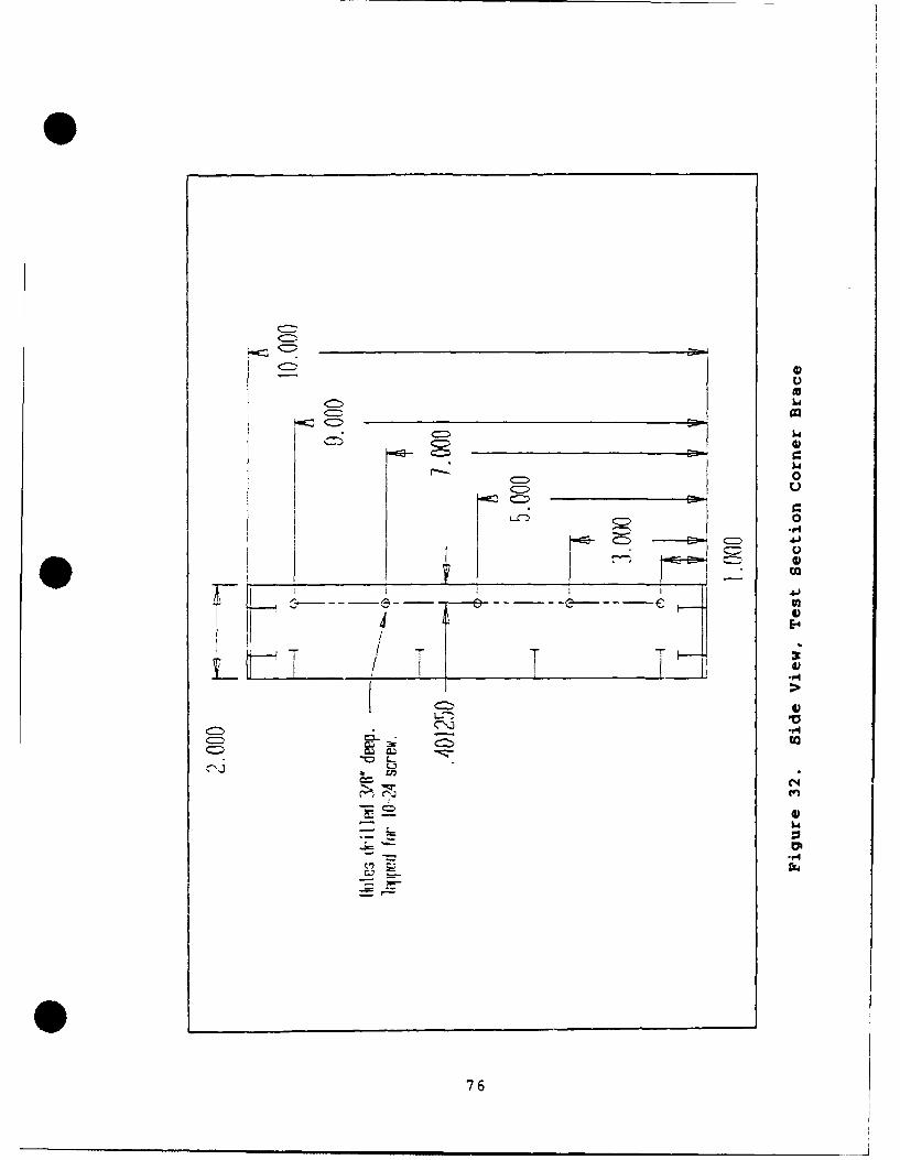
C=) 10

C=) 0cz:)E3- => A

4C

__72

16-

0

a..r4

-

0.-00

4

U-,-4

77 4

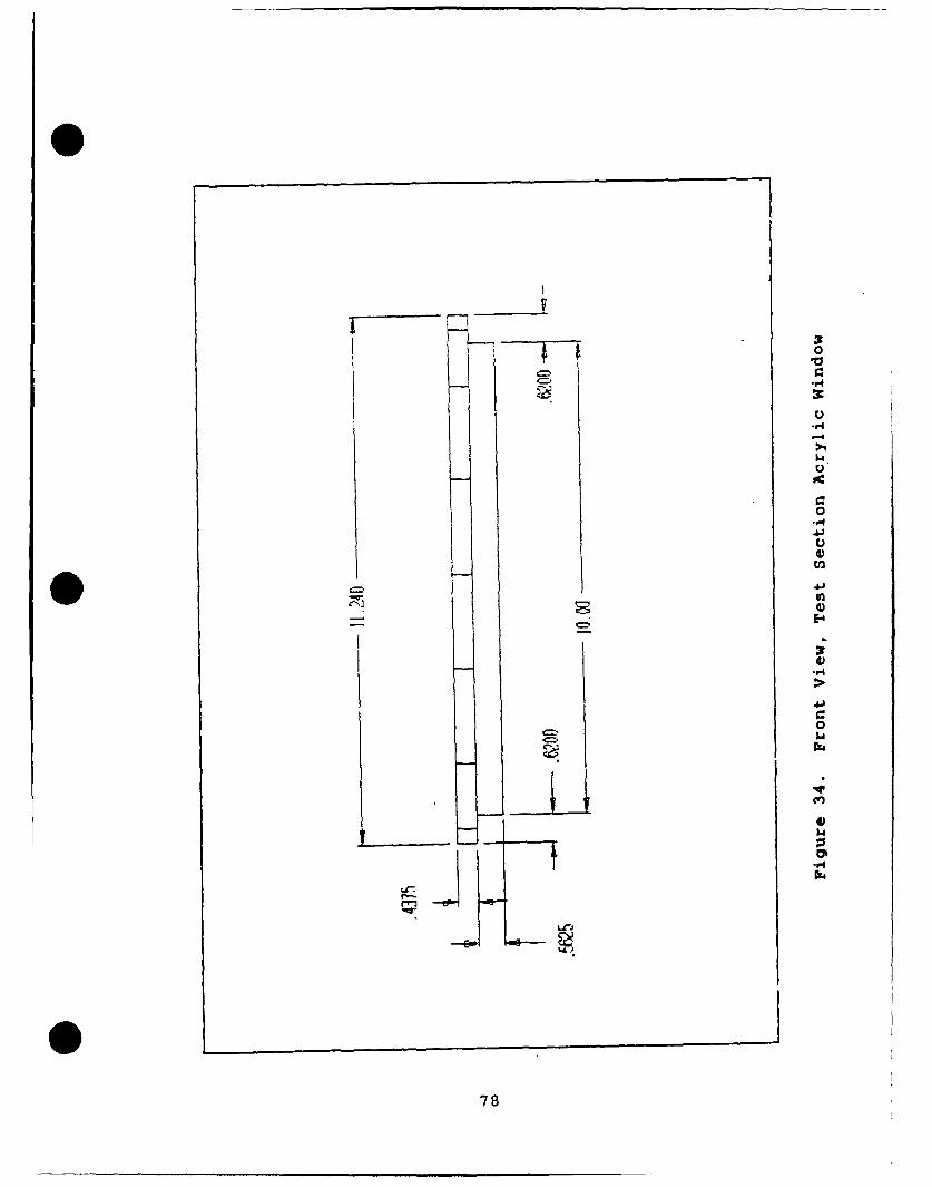
0

E-4

0

a,

ru

S a)

4'

-do-

0

* I

78

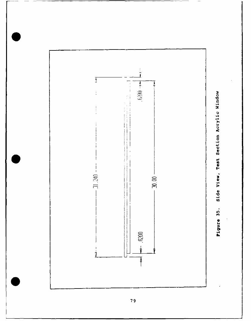
00

U

0

IID

ofI

-1-

79

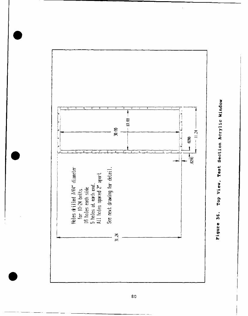
00 0 0

a, a

run

-= cn

co PA

L2 C-

a.~CcI

- ~.94- e~j o~b4

I r80

-r

0

* -7ri C= 0

TN 7

81.

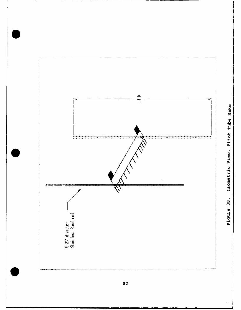
idP

A4 o

alp FK%

/~-A-/

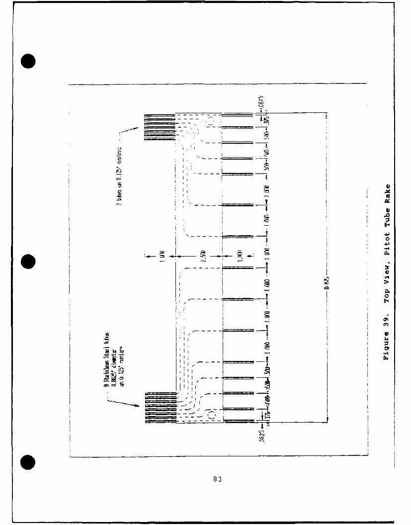
'I-'

S -

_________________________________ a

-----

--- = - - -=

A I. i

I -.

4~

I - I I 0

------- ~ I

I I I '

-- -4 04.)

~ -u--.- r4

* -I -

S~V

-'.4

I

- - - -I '0

I, I

K;-

C')

I -1 6~I I

I ILii -'.4

---

IIII,

II

- I

I rI I

~. , /I - - -

-i.. ~- - -~__

- - I

- - --- 1 1

~.r)

c-J

83

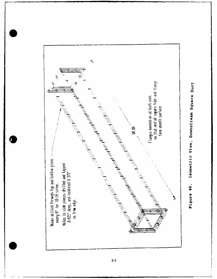
4.".

AV))

N Ot

w -=R =

cu- 2-. 0wN*:

84N

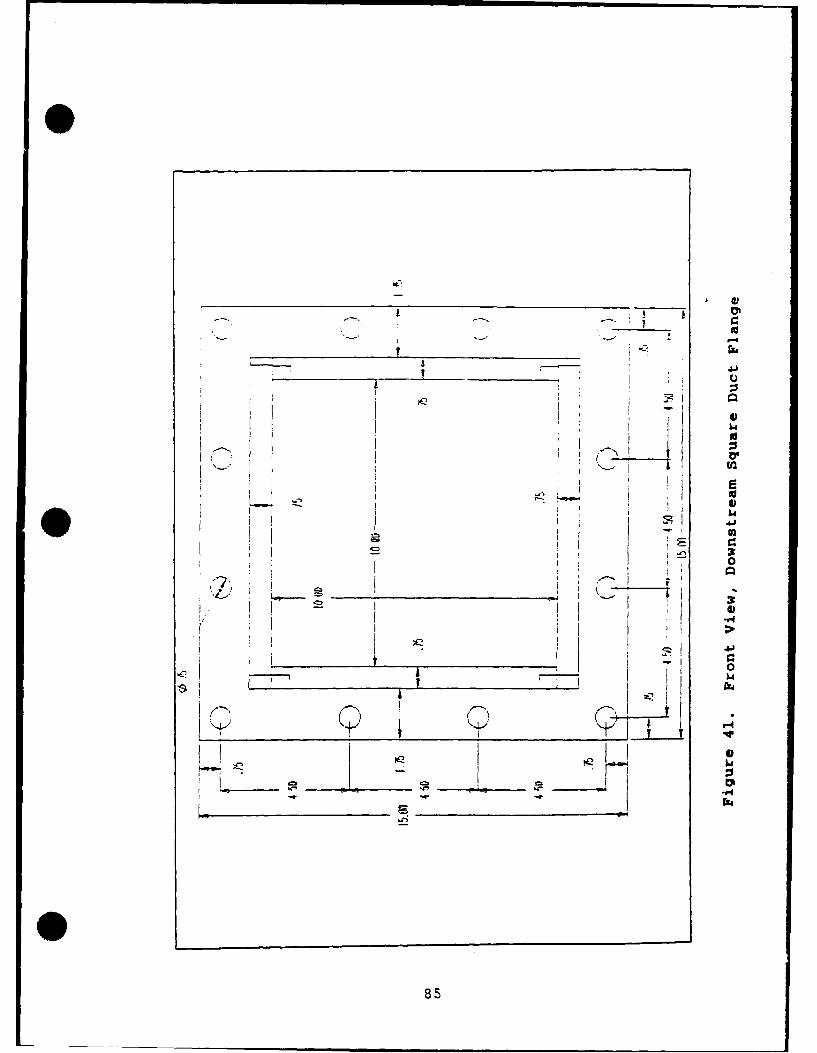
___ Va

0

__________________

~Zd

-_______ _______

C.)

I I -. El

K~KI

.-~.-...\t

I'-,.. C12

Li 0j~.d

* I El.4J

-.~

0

I?

2 II

i~) El

I I I

K El

ra~

85

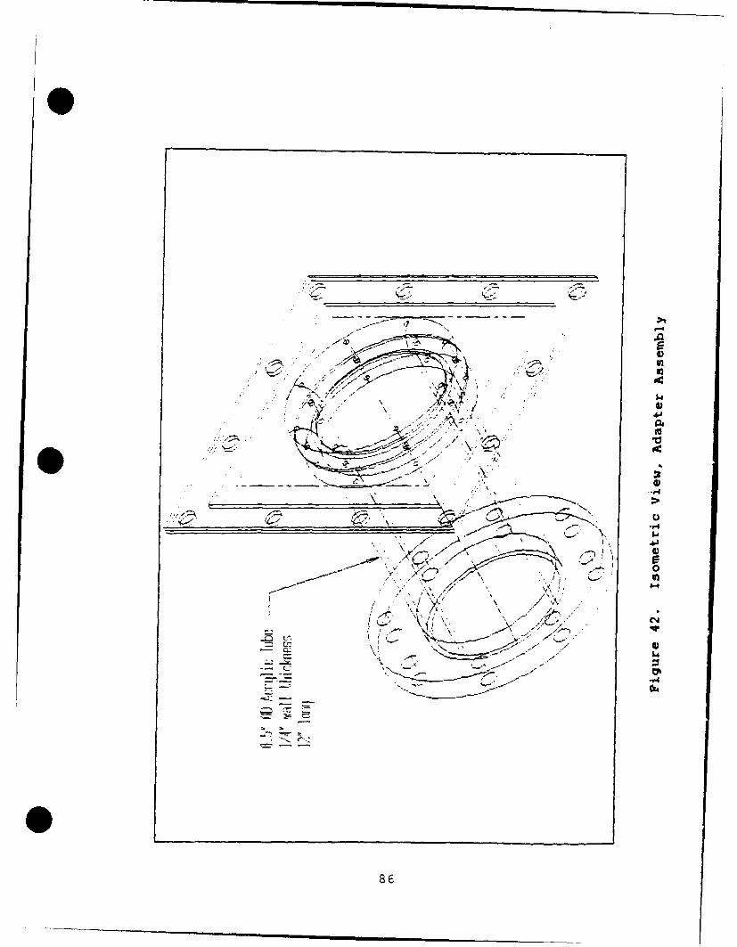
/o- ,

"'- -

... .-- *,_.-- ... . . "' .. "

S _--.-* .- , ,/ ~

',- .. . . \ .. .-

....-.,._ , .-- L , , .

. - """ " > ' A ,,S ," ' N

- -. - . , -- , ,.

".'- -',5'-i mu m-i mu nlnLma

V4

- 0k

( f I

87 -

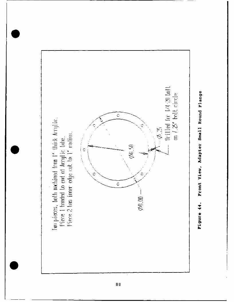
@3

C-

'U

C-~

-- - N 0- ,~ , N

-- C- -

-~ ... '-.~ --

- Er -

-- - I

-~ L.U-;. @3

-- .

0U- L~L~ -~

2I- @3

/

-,--- C~ -b a~ ..- 0

I- I.d

~ c -- ~

-~= c~ _ cc.

C.2 @3

-- C-2

-- -- oh- U- U-- -v.4-c

88

E

'.

_

I' /.

I,..

El

894

I I I II I-

0a

0

VN

N~K 0N Li"N

-~

K 040

N'K

0C C ~

' Li/

.- 0./ / - \ / 0-c I

/

/~ // -

/( *u-4

-~ /1 / -'4Li

/ .1-I4,-

0U

'-4

~0

4.

El

La

*1*4

90

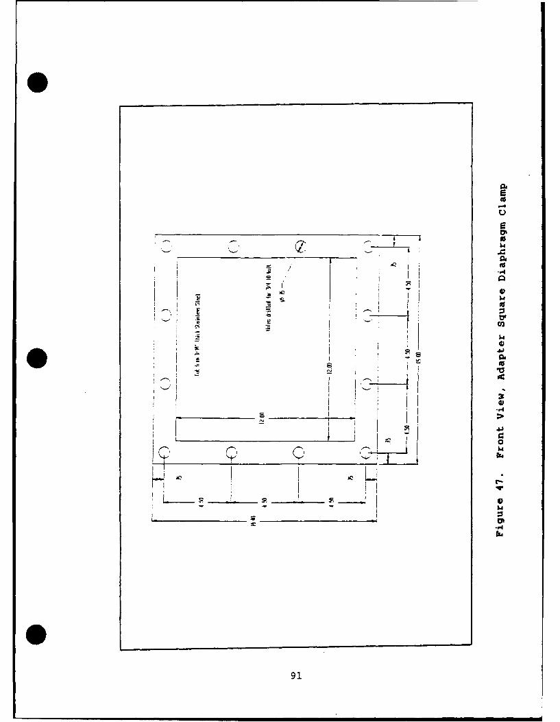
-4

919

Appendix B - FORTRAN Program for Calculation of Velocity

Field Around Sphere in Rectangular Tunnel

CC Calculate Velocity at points around a SphereC in a Rectangular Tunnel, Velocity due to:C -Uniform StreamC -Doublet Potential Flow (Karamcheti, p. 339-340)C -Doublet Images (Pope, p. 348)C -Sources and Sinks on Centerline (Karamcheti, p. 322)C INPUT: N size of doublet image array NxNC N=1 corresponds to infinite field (no tunnel effect)C B Tunnel width [ft]C H Tunnel height [ft'C D Diameter of sphere [ft]C U Free stream velocity [ft/sec]C P number of pointsC x(!...p), Y(I.. .p),Z(I... p) coordinates of pointsC mu Strength of DoubletC xsrc Location of Sources and SinksC qsrc Strength of Sources and Sinks********************************************** ******* ******

integer Preal muparameter( pi= 3.141592654 )dimension xd(201),yd(201),zd(201)dimension x(2000),y(2000),z(2000),Vx(2000),Vy(2000)dimension Vz(2000), xsrc(100),qsrc(100)character*20 infiln,outfillogical dblt,src

write(*,*) ' Enter Input File Name'read(*,6) infiln

6 format(A20)write(*,*) ' Enter Output File Name'read(*,6) outfilprint*,' Use doublet at x=0? [ .T. or .F. J'read*,dbltprint*,' Enter Number of Sources and Sinks'read*,nsrcif (nsrc .gt. 0) thenprint*,'" Location [inch], Negative is Upstream'print*, ' Iprint*,'? Strength [Multiple of Doublet Strength]'print*,' Positive for Source, Negative for Sink'endif

do 110 i=l,nsrc

92

print*,' Enter Location',ir ead* ,xs r c (,)xsrc(i) = xsrc(i)/12.Oprint*,' Enter Strength',iread* ,qsrc(4i)c OntL.nu e

open(7,fileinf iln,status='old')read(7 ,1) N,B,H,D,U-

Sformat(13,4(1x,F10. 6))

C Read coordinates of points in tunnelread(7,*) Pread(7,2) (x(i) ,y(i) ,z(i) ,i=1,p)close (7)print*,'Images:',N,'Width,Height:',B,H,'Dianeter-:'

+ D,'Uinf:',TJ2 f-orrnat(3F11!.6)

C Generate Grid points for Doublet and Doublet Imagesopen(8,file=outfil,status='new')write( 8,1) N ,B,H,. , T7

do 10 i1l,nxd(i)= 0yd(i)= B* (i4-int(n,'2)-1)zd(i)= H* (i-int(n/2)-l)

IC c o.-t -'n -ue

mu= U*2*pi*(D/2)**3

write(*,*) "'p:"' ,p

write(8,*) "'Velocity [ft/sec] at P(x,y,z)"'

+ I *IFVZI I It fi rIII

3 format(A4,7(A1O))C Calculate Velocity at the p points

do 20 i=l,pVx(i)= UVy(i)= 0Vz(i)= 0do 30 k1l,N

do 40 j1l,Nrx= x(i)ry= y(i) - yd(j)rz= z(i) - zd(k)rho2= ry**2 + rz**2R= sqrt(rx**2 + ry**2 + rz**2)if ((R.lt.1.Oe-03) .or.

+ ((rx-xsrc(m))**2+rho2).lt.l.0e-03 )thenVx(i)= 0Vy(i)= 0Vz(i)= 0

93

goto 30end i f

C Add Doublet effect for Sphereif (dblt) then

Vx(ij)= Vx(ij) +mu*( rho2/2-~rx**2 )/ (2*pi*R**5)Vy(i ) Vy(i )-3*mu*rx*ry/ (4*pi*R**5)Vz(i)= Vz(i )-3*mu*.-x*rz/ (4*pi*R**5)endif

C Add! Sink and Source effects for wakedo 100 rnzl,nsrc

qvel= Tu*qsrc (i) /(4. 0*pi )/+ ( (rx-xsrc(m))**2 + rho2 )**1.5

Vx(i)= Vx(i)-;- qvel* (rx-xsrc(m))Vy(i)= Vy(i)+ qvel* ryVz(i)= Vz(i)+ qvel* rz

'100 continue40 continue30 continue

V= sqrt(Vx(i)**2 + Vy(i)**2 +- Vz(i)**2)write(8,4) i,x(i)*12.0,y(i.)*12.0,z(i)*12 .0,

+ Vx(i) ,Vy(i) ,Vz(i) ,Vwrite(*,5) '+record ',i,' of ',p,'writt.eni'

4 f.orrat(14,7(lx,F1O.6) )5 format(A8, 14,A4,14 ,A7)20 cont inue

close( 8)stop

E "

94

Appendix C - Acrylic Window Structural Analysis

The material chosen for the side walls of the water

tunnel test section is acrylic sheet of nominal one -::ch

thickness. This material is a thermoplastic also known as

polymethylmethacrylate or by the trade names lucite and

plexiglas. Acrylic has the following physical properties

[5] relative to its use in this research facility:

Table 1. Physical Properties of Acrylic Plastic

Tensile Strength 7,000 - 11,000 ps:

Compressive Strength 11,000 - 17,000 psi

Young's Modulus 350,000 - 500,000 psi

Specific Gravity ".17 - 1.20

Poisson's ratio was not reported for this material so a

value of 0.3 was assumed. The minimum reported value of

350,000 psi for Young's modulus is used in the following

analysis.

Preliminary analysis was performed using formulae for

the stress and deflection of a thin plate under a pressure

load on one side [32:386,393]. The configuration, loading,

and boundary conditions of the acrylic window did not quite

fit any of the limited number of cases for which formulas

were provided so the NISA II PC [6] finite elements analysis

* computer program was used to provide a more refined

analysis.

95

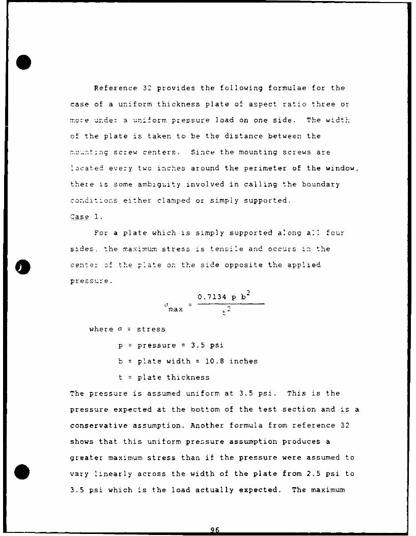
Reference 32 provides the following formulae for the

case of a uniform thickness plate of aspect ratio three or

mcre under a uniform pressure load on one side. The width

of the plate is taken to be the distance between the

----nt-ng screw centers. Since the mounting screws are

located every two inches around the perimeter of the window,

there is some ambiguity involved in calling the boundary

conditions either clamped or simply supported.

Case 1.

For a plate which is simply supported along a'l four

sides, the maximum stress is tensile and occurs in the

center of the Iate on the side opposite the applied

pressure.

0.7134 p b2

max ZI

where a = stress

p pressure = 3.5 psi

b plate width = 10.8 inches

t = plate thickness

The pressure is assumed uniform at 3.5 psi. This is the

pressure expected at the bottom of the test section and is a

conservative assumption. Another formula from reference 32

shows that this uniform pressure assumption produces a

greater maximum stress than if the pressure were assumed to

vary linearly across the width of the plate from 2.5 psi to

3.5 psi which is the load actually expected. The maximum

QFi

deflection also occurs at the center of the plate and is

given by

0.1335 p b3

Yrax= E t3

where y = deflection

E = Young's modulus = 350,000 psi

Case 2

For a plate which is clamped along all four sides, the

maximum stress is again tensile and occurs in the center of

the longest edge, on the clamped boundary on the same side

of the plate as the applied pressure. This stress is given

0.5 p b2

max t2

The maximum deflection is again at the center of the plate

and is

0.0284 p b4

Ymax

E t

Summary_ of Preliminary Analysis

The nominal one inch thick acrylic plate has an actual

minimum thickness of 0.96". Because the thickness

varies by as much as 0.040" throughout the plate, the

minimum thickness of the flange which supports the window is

0.30".

97

The following shows the result of eva'uating the

formulae given abcve at both thicknesses.

Taea 2. Summay of Stress on Thin Acrylic PLate

Ecundar-y Thickness Stress Deflection'inches] [psi] [inches]

simply supForted 0.30 3,236 0.673

simply supported 0.96 316 0.021

c.amped 0.30 2,268 0.143

clamped 0.96 221 0.004

:t is obvious from these results that the window would be

sufficiently strong if it were 0.96" thick throughout.

Since the window has a 0.30" thick flange along the entire

perimeter, however, it is noted that the maximum stress for

a 0.30" thick plate is of the same order of magnitude as

the maximum allowable stress ( 7,000 psi). Also, the maximum

stress is likely to occur near the edge of the window, which

is where the corner of the flange is located, and such a

corner is a known stress concentration factor. This

indicates that a more rigorous analysis is needed, and a

finite element analysis of the window is presented next.

The results of the above analysis for the 0.96" thick

plate with a clamped boundary are used to validate the

finite element model of the window as explained in the next

section.

NISA Finite Element Ana sis

The window was modeled using three dimensional solid

elements with nodes at each corner and at the midpoints of

the edges for a total of twenty nodes per element. Only

one-quarter of the window was modeled, and symmetric

boundary conditions were applied at the appropriate

boundaries. Many of the elements had rather large aspect

ratios, but the elements near the edges were nearly square.

Even with the large elements and the symmetry technique,

this model was near the upper limit of model complexity

possible on the personal computer version of NISA available.

The first model used was that of a plain plate, the

purpose being to compare results to the preliminary results

reported in the previous section. A diagram of the cross

section of the model, not to scale, follows.

applied pressure 3.5 psi

symmetric clamped

edge edge

Figure 48. Cross Section of Finite Element Modelof Flat Plate

The maximum deflection computed was 0.004" at the

99

center of the plate which is the same as the estimate

in Table 2. The maximum stress was 237 psi tension

at the center of the longest edge on the same side of the

plate as the applied pressure, and the maximum compressive

stress was -262 psi at the side of the plate opposite the

applied pressure. The magnitude of these stress values is

7.2% higher and 18.5% higher, respectively, than the

corresponding estimates in Table 2 above and in neither case

is the comPuted stress as large as that estimated for the

simply supported edge case above. So it seems that the

large aspect ratio elements used in the central portion of

the finite element model have not seriously degraded the

results obtained.

The finite element model for the window is obtained

from the plate model by deleting certain elements as can be

seen in Figure 49 below. Note that only a cross section of

the model is shown, and the model is in fact composed of

three dimensional elements. The flange on the long edge can

applied pressure 3.5 psi

symmetric

edge -_ clampededge

Figure 49. Cross Section of Finite Element Modelof Window

be seen in the figure, and while the flange on the short

100

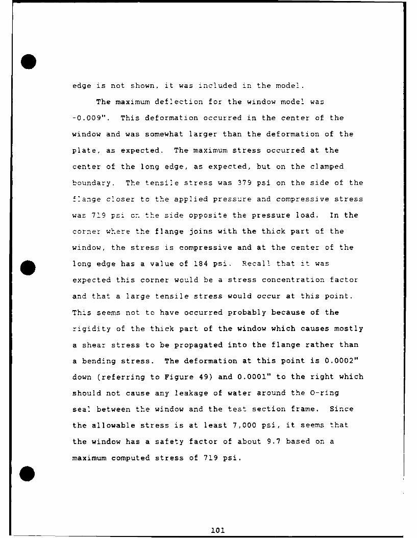
edge is not shown, it was included in the model.

The maximum deflection for the window model was

-0.009". This deformation occurred in the center of the

window and was somewhat larger than the deformation of the

plate, as expected. The maximum stress occurred at the

center of the long edge, as expected, but on the clamped

boundary. The tensile stress was 379 psi on the side of the

f:ange closer to the applied pressure and compressive stress

was 719 psi on the side opposite the pressure load. In the

corner where the flange joins with the thick part of the

window, the stress is compressive and at the center of the

long edge has a value of 184 psi. Recall that it was

expected this corner would be a stress concentration factor

and that a large tensile stress would occur at this point.

This seems not to have occurred probably because of the

rigidity of the thick part of the window which causes mostly

a shear stress to be propagated into the flange rather than

a bending stress. The deformation at this point is 0.0002"

down (referring to Figure 49) and 0.0001" to the right which

should not cause any leakage of water around the O-ring

seal between the window and the test section frame. Since

the allowable stress is at least 7,000 psi, it seems that

the window has a safety factor of about 9.7 based on a

maximum computed stress of 719 psi.

101

A6ppendix D - Nozzle Design

The problem to be addreszed in designing a nozzle fcr

this research pioject is that a relatively slow flow of

circular cross section must be accelerated to a fast flow of

square cross section which is as uniform as possible.

First, the flow in the 24" diameter stilling tank is assumed

uniform as is the flow in the 10" square test section.

Then, smooth polynomial curves are used to mate the

circular cross section to the square cross section.

The polynomials used to define the shape of the nozzle

have zero slope in the longitudinal direction at either end

of the nozzle and have an inflection point along the length

of the nozzle at a specified location. Since the boundaries

of the nozzle can be generated by simple polynomials, and

are streamlines (actually stream surfaces), it is possible

to derive a stream potential and a velocity potential for

flow inside the nozzle although this will not be shown in

this thesis. According to Professor Larsen [24], this

method has often been used to design both internal flow

diffusers and nozzles and external flow aircraft fuselage

and nacelle parts where some specified shape must be

enclosed by a smooth curved surface.

Consider the graph of a smooth curve as shown in Figure

0 50 where the slope of the curve at x = 0 and at x L is

102

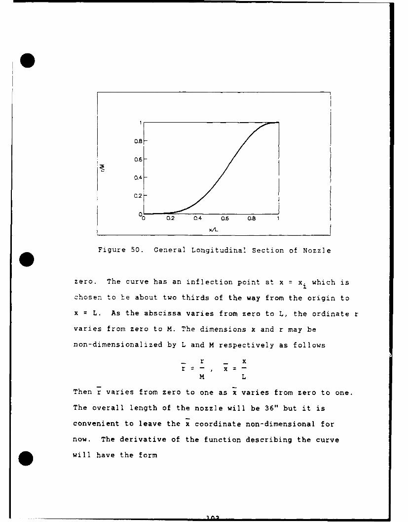
0.8

0.4-

C.2K

0 0.2 0.4 0.6 0.8 1

x/L

Figure 50. General Longitudinal Section of Nozzle

zero. The curve has an inflection point at x = x. which is

chosen to he about two thirds of the way from the origin to

x = L. As the abscissa varies from zero to L, the ordinate r

varies from zero to M. The dimensions x and r may be

non-dimensionalized by L and M respectively as follows

- r _ xr:-, x = -

M L

Then r varies from zero to one as x varies from zero to one.

The overall length of the nozzle will be 36" but it is

convenient to leave the x coordinate non-dimensional for

now. The derivative of the function describing the curve

*will have the form

dr

dx

where q must be an integer in order to keep the remaining

analysis simple, and p may be any real number. The

constant k will be evaluated later. The second derivative

of r(x) will be

2-d r k p-( 1 x )q -Pq(l-x) p - I

dx2I

Now set the second derivative equal to zero and the

resulting value of x will be x, the value at the inflection

point.

C = kxpI-x) - p(l-xi) - qx i

The roots of this equation at x = 0 and x = 1 are not of

interest so solve the equation for x. resulting in

0 = p(l-x i ) - qx i

_ px. = -

1 q+p

Since we desire x. to be about two-thirds, and q must be an

integer, set q = 2. Then a value of p = 3.5 will give

x. = 0.636.1

Substituting q 2 into equation (1) and integrating

produces

k 2k kr- xP+ -xp+2 +- x-p+3 + C

p+l p+ 2 p+3

104

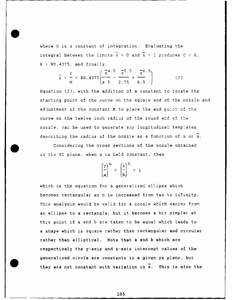
where C is a constant of integration. Evaluating the

integral between the limits x 0 and x = 1 produces C = 0,

k = 80.4375, and finally4.5 -5.5 -6.

r- - 80.4375 4 x 6.51

M 4.5 2.75 6.5

Equation (2), with the addition of a constant to locate the

starting point of the curve on the square end of the nozzle and

adjustment of the constant M to place the end point of the

curve on the twelve inch radius of the round end of the

nozzle, can be used to generate any longitudinal templates

describing the radius of the nozzle as a function of x or x.

Considering the cross sections of the nozzle obtained

in the YZ plane, when x is held constant, then

c In + [n= 1

which is the equation for a generalized ellipse which

becomes rectangular as n is increased from two to infinity.

This analysis would be valid for a nozzle which varies from

an ellipse to a rectangle, but it becomes a bit simpler at

this point if a and b are taken to be equal which leads to

a shape which is square rather than rectangular and circular

rather than elliptical. Note that a and b which are

respectively the y-axis and z-axis intercept values of the

generalized circle are constants in a given yz plane, but

they are not constant with variation in x. This is also the

105

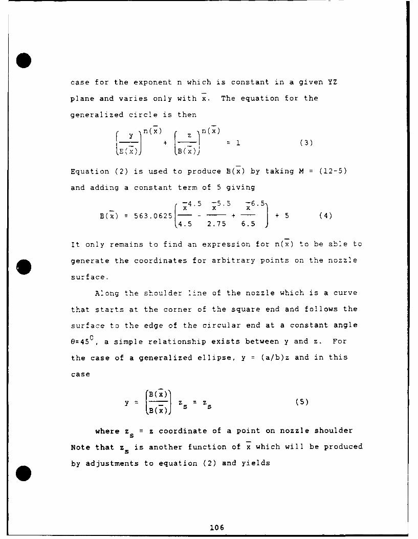
case for the exponent n which is constant in a given YZ

plane and varies only with x. The equation for the

generalized circle is then

B(x)= 1 (3)

Equation (2) is used to produce B(x) by taking M = (12-5)

and adding a constant term of 5 giving

S4.5 5.5 X -6.5B(x) = 563.0625 - - + - + 5 (4)

4.5 2.75 6.5

It only remains to find an expression for n(x) to be able to

* generate the coordinates for arbitrary points on the nozzle

surface.

Along the shoulder line of the nozzle which is a curve

that starts at the corner of the square end and follows the

surface to the edge of the circular end at a constant angle

e=450, a simple relationship exists between y and z. For

the case of a generalized ellipse, y = (a/b)z and in this

case

y - z z (5)

where z = z coordinate of a point on nozzle shoulder

Note that z is another function of x which will be produced

by adjustments to equation (2) and yields

106

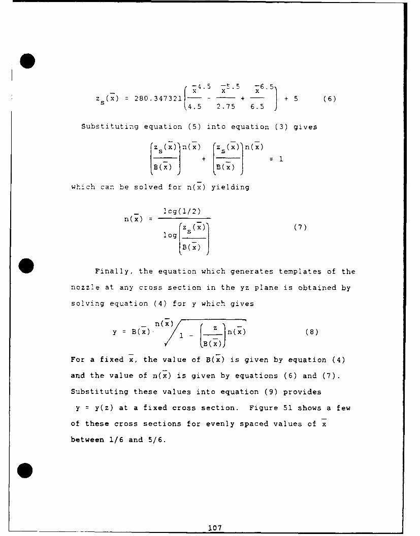
4. E 5 x6.5,zs (X) = 280.34732"- - + - + 5 (6)

84.5 2.75 6.5

Substituting equation (5) into equation (3) gives

z(x)n( {'sx)jn(x

which can be solved for n(x) yielding

lcg(1/2)n(x) =

log Zs(X) (7)

Finally, the equation which generates templates of the

nozzle at any cross section in the yz plane is obtained by

solving equation (4) for y which gives

y = B(x) n[-) r z n(x) (8)

For a fixed x, the value of B(x) is given by equation (4)

and the value of n(x) is given by equations (6) and (7).

Substituting these values into equation (9) provides

y = y(z) at a fixed cross section. Figure 51 shows a few

of these cross sections for evenly spaced values of x

between 1/6 and 5/6.

107

12

4-

% 2 4 6 8 10 12

Z fthaw

Figure 51. Cross Sections of Nozzle at Evenly SpacedLongitudinal Stations

Recall that Equation (2) can be adjusted to describe

longitudinal templates for this nozzle. These template

curves will lie in any plane which contains the

center line of the nozzle. It can be shown that these

curves will be of the form

B(x) 1 1 inxR(x) - (9)

cose l+tann(x)J

where R(x) = radius from center line of nozzle

e angle in the YZ plane away fromy-axis or z-axis

B(x) and n(x) will be developed next

108

The angle e in equation (9) should only be allowed to vary

between 00 and 450. This causes no great difficulties as

the nozzle symmetry can be exploited so that a set of

templates which covers one-eighth of the nozzle can be used

on the other octants as well.

Equation (9) is also be used to find the maximum slope

n the nozzle. The nozzle designed for this research

project has a maximum slope of 23.03 which occurs at four

locations corresponding to 0 = 0 (the y-axis and z-axis) and

_s at the same longitudinal location as the inflection

point. The nozzle length is 36" so when x 0.636, and1

note that the inflection point occurs at x. = 0.636 no

matter what the angle 6 is, then x = (0.636)(36") = 22.9".

Since anadverse pressure gradient in the flow

direction is not expected in a nozzle as it is in a

diffuser, the maximum slope of 23.030 is not expected to

cause any stalled regions in the nozzle. If this technique

is used to design any diffusers for future modifications to

this research facility, it is important to note thit this

design procedure provides no benefit as far as designing

diffusers with large flow turning angles which are any less

likely to experience separated flow. This process is

presented solely as a technique to mate a round cross

section flow with a square cross section flow.

11

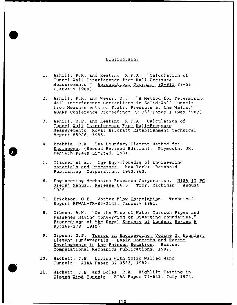
Bibli ography

1. Ashill, P.R. and Keating, R.F.A. "Calculation ofTunnel Wall Interference from Wall-PressureMeasurements," Aeronautical Journal, 92-911:36-53(January 1988)

2. Ashill, P.R. and Weeks, D.J. "A Method for DeterminingWall Interference Corrections in Solid-WaMl Tunnelsfrom Measurements of Static Pressure at the Walls,"AGARD Conference Proceedings CP-335:Paper 1 (May 1982)

3. Ashill, R.P. and Keating, R.F.A. Calculation ofTunnel Wall Interference From Wall-PressureMeasurements, Royal Aircraft Establishment TechnicalReport 85086, 1985.

4. Brebbia, C.A. The Boundary Element Method forEngineers, (Second Revised Edition). Plymouth, UK:Pentech Press Limited, 1984.

5. Clauser et al. The Encyclopedia of EngineerinngMaterials and Processes. New York: ReinholdPublishing Corporation, 1963.963.

6. Engineering Mechanics Research Corporation. NISA II PCUsers' Manual, Release 86.6. Troy, Michigan: August1986.

7. Erickson, G.E. Vortex Flow Correlation. TechnicalReport AFWAL-TR-80-3143, January 1981.

8. Gibson, A.H. "On the Flow of Water Through Pipes andPassages Having Converging or Diverging Boundaries,"Proceedings of the Royal Society of London, Series A83:366-378 (1910)

9. Gipson, G.S. Topics in EnQineering, Volume 2, BoundaryElement Fundamentals - Basic Concepts and RecentDevelopments in the Poisson Equation. Boston:Computational Mechanics Publications, 1987.

10. Hackett, J.E. Livin~g with Solid-Walled WindTunnels. AIAA Paper 82-0583, 1982.

11. Hackett, J.E. and Boles, R.A. Highlift Testing inClosed Wind Tunnels. AIAA Paper 74-641, July 1974.

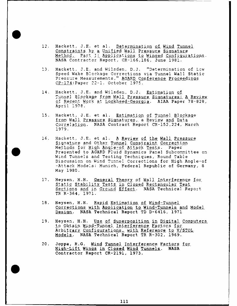
12. Hackett, J.E. et al. Determination of Wind TunnelConstraints by a Unified Wall Pressure Signature

Method. Part I: Applications to Winged Configurations.NASA Contractor Report, CR-166,186, June 1981.

13. Hackett, J.E. and Wilsden, D.J. "Determination of LcwSpeed Wake Blockage Corrections via Tunnel Wall StaticPressure Measurements," AGARD Conference ProceedingsCP-174:Paper 22-1. October 1975.

14. Hackett, J.E. and Wilsden, D.J. Estimation ofTunnel Blockage from Wall Pressure Signatures: A Reviewof Recent Work at Lockheed-Georg a. AIAA Paper 78-828,April 1978.

15. Hackett, J.E. et al. Estimation of Tunnel Blockagefrom Wall Pressure Signatures1 a Review and DataCorrelat-on. NASA Contract Report CR-152,224, March1979.

16. Hackett, J.E. et al. A Review of the Wall PressureSignature and Other Tunnel Constraint CorrectionMet'ods for High A nge-of Attack Tests. PaperPresented to AGARD Fluid Dynamics Panel Subcommittee onWind Tunnels and Testing Techniques, Round TableDiscussion on Wind Tunnel Corrections for High Angle-of-Attack Models: Munich, Federal Republic of Germany, 8May 1980.

17. Heysen, H.H. General Theory of Wall Interference forStatic Stability Tests in Closed Rectangular Test

Sections and in Ground Effect. NASA Technical ReportTR R-364, 1971.

18. Heysen, H.H. Rapid Estimation of Wind-TunnelCorrections with Application to Wind-Tunnels and ModelDesign. NASA Technical Report TD D-6416, 1971

19. Heysen, H.H. Use of Superposition in Digital Computersto Obtain Wind-Tunnel Interference Factors forArbit-rar Configurations, with Reference to V/STOLModels. NASA Technical Report TR R-302, 1969.

20. Joppa, R.G. Wind Tunnel Interference Factors forHigh-Lift Wings in Closed Wind Tunnels. NASAContractor Report CR-2191, 1973.

111

21. Karamcheti, K. Princiles of Ideal-FluidAerodynamics. Malabar, Florida: Robert E. KriegerPublishing Company, :ncorporated, 1.980.

22. Kline, S.J. "On the Nature of Stall," Journal of BasicEngneering 81:305-320 (September 1959)

23. Kline, S.J. et al. "Optimum Design of Straight-WalledDiffusers," Journal of Basic Engineering 81:321-331(September 1959)

24. Larsen, H.C., Professor Emeritus of Aerospace Veh:cleDesign, School of Engineering, Air Force Institute ofTechnology, Wright-Patterson AFB, Ohio. Personal:nterviews, 13 June through 30 September 1988.

25. Maskell, E.C. A Theor of the Blockage Effects onBluff Bodies and Stalled Win.gs in a Closed Wind Tunnel.Air Research Committee (United Kingdom), Reports &Memcranda Number 3400, 1963.

26. Moses, D.F. "Wind Tunnel Wail Corrections Deduced byIterating from Measured Wall Static Pressure" AIAAjournal 21:1667-1673 (December 1983)42

27. Newman, P.A. and Barnwel, R.W. Wind Tunnel WallInterfe renc eCorrection. NASA Conference PublicationCP-2319, January 1983.38

28. Pirolo, Capt D.G. Piezoelectric Polymer Tactile SensorArrays for Robotics. MS Thesis, AFIT/GE/ENG/87D-52.School of Engineering, Air Force Institute ofTechnology (AU), Wright-Patterson AFB, OH, December1987.

29. Rae, W.H. Jr. and Pope, A. Low-Speed Wind TunnelTesting (Second Edition). New York: John Wiley &Sons, Incorporated, 1984.

30. Reston, Capt R.R. Robotic Tactile Sensor Fabricatedfrom Piezoelectric Polyvinylidene Flouride Films. MSThesis, AFIT/GE/ENG/88D-41. School of Engineering,Air Force Institute of Technology (AU),Wright-Patterson AFB, OH, December 1988.

31. Rauscher, M. Introduction to Aeronautical_ Pynamics.New York: John Wiley & Sons, Incorporated, 1953.

32. Roark, R.J. and Young, W.C. Formulas for Stress andStrain (Fifth Edition). New York: McGraw-Hill BookCompany, 1975.

112

33. Stahl, W.H. Variable-Temperature Water Tunnel for Hi-ghReynolds Numbers. AIAA Paper 85-0051, January 1985.

34. Streby, G.D. Multi-Ducted Inlet Combustor Research andDevelopment interim Technical Report, August 1981 toAugu;st 982. Contract F33615-82-C-2074(SB5448-82-C-0518), Air Force Wright AeronauticalLaboratories, Aero Propulsion Laboratory, TechnicalReport AFWAL-TR-82-2101, October 1982.48

35. Streeter, V.L. and Wylie, E.B. Fluid Mechanics,

(Seventh Edition). New York: McGraw-Hill Book Company,1979.

36. Walker, A.S. and Wiseman, N.P. The Pressure Sinature

Method for Blockage Correct ions and Its Application tothe Industrial Wind Tunnel. BS Thesis, BU-263.Department of Aeronautical Engineering, University ofBristol, June 1981.

37. Zhou, C. Integral Method of Wall InterferenceCorrection in Low-Seed Wind Tunnels. NASA Technical

Translat-ion of "Disu Fendong Dongbi Ganrao Xiuzheng DiJifen Fangfa," Kongqi Lixue Xuebao, Number 2:1-8 (June1985). NASA-TT-20055, April 1987.

113

V ITA.

Kurt A. Lautenbach -"

He received an Associate in

Applied Science degree in Mental Health and Social Services

from Philadelphia Community College in March 1977 and a

Bachelor of Science in Chemistry from Saint Joseph's

University, Philadelphia in May 1980. He was commissioned

through Officer Training School at Lackland Air Force Base,

Texas on 15 July 1981 and assigned to the Air Force

Institute of Technology for the Undergraduate Engineering

ConVersion Program where he earned a Bachelor of Science in

Aeronautical Engineering in March 1983. He was then

assigned to Air Force Systems Command, Electronic Systems

Division at Hanscom Air Force Base, Massachusetts where he

worked in the Jam-Resistant Voice Communications

Systems Program Office first as an Aircraft Integration

Project Officer and eventually as HAVE QUICK II High Power

Amplifier Program Manager. He entered the Air Force

Institute of Technology in the Graduate Aeronautical

Engineering Program in June 1987.

11

UNCLASSIFIEDSECURITY CLASSiFfCATION OF THIS PAGE

I Form ApprovedREPORT DOCUMENTATION PAGE OMB No. 0704-0188

la REPORT SECURITY CLASSIFICATION lb RESTRICTIVE MARKINGSUNCLASSIFIED

2a. SECURITY CLASSIFICATION AUTHORITY 3 DISTRIBUTION/AVAILABILITY OF REPORTApproved for public release;

2b. DECLASSIFICATION /fDOWNGRADING SCHEDULE distribution unlimited

4. PER"OR.%%G O 9C-_1%!ZATION PEoORT NUMBER(S) 5. MONITORING ORGANIZATION REPORT NUMBER.(S)

AFIT/GAE/AA/88D-20

6a. NAME OF PERFORMING ORGANIZATION 6b. OFFICE SYMBOL 7a. NAME OF MONITORING ORGANIZATION(if applicable)

School of Engineering AFIT/ENY _ _'__ _ _ _ _

6c. ADDRESS (City, State, and ZIP Code) 7b. ADDRESS (City, State, and ZIP Code)

Air Force Institute of TechnologyWright-Patterson AFB, OH 45433-6583-/V

8a- NAME OF FUNDING /SPONSORING Bb OFFICE SYMBOL 9 PROCUREMENT INSTRUMe1NT ID A (")ATION NUMBER

ORGANIZATION (if applicable)

8c ADDRESS (City, State, and ZIP Code) 10 SOURCE OF FUNDING NUMBERS

PROGRAM PROJECT TASK WORK UNITELEMENT NO. NO. NO ACCESSION N

1. TITLE (Include Security Classification)

esign of Water Tunnel to Measure Wall Pressure SignaturesDue to Tunnel Blockage and Wake Effects

12. PERSONAL AUTHOR(S)

Kurt A. Lautenbach, B.S.. Capt. USAF13a. TYPE OF REPORT 13b. TIME COVERED 14. DATE OF REPORT (Year, Month, Day) 15 PA E COUNT

MS Thesis FROM TOI ng r pmhpr16. SUPPLEMENTARY NOTATION

17. COSATI CODES 18 SUBJECT TERMS (Continue on reverse if necessary and identify by block number)

FIELD GROUP SUB-GROUP

14 02 Water Tunnel01 01 Wind Tunnel Tptcf

19. ABSTRACT (Continue on reverse if necessary and identify by block number)

Thesis Advisor: Maj Lanson J. Hudson, USAFInstructorDepartment of Aeronautics and Astronautics

This thesis describes the design and construction of a new testsection for the AFWAL Aero Propulsion Lab six-inch water tunnel inbuilding 18. The new test section has a ten-inch square cross sectionand is designed to measure wall pressure signatures caused by solid andwake blockage of the flow due to the separation bubble which forms aroundbluff bodies immersed in the flow. The wall pressure signature for aspherical model is predicted. Applications of the method and associatedrequirements for instrumentation are discussed.

20. DISTRIBUTION /AVAILABILITY OF ABSTRACT 21. ABSTRACT SECURITY CLASSIFICATION

] UNCLASSIFIED/UNLIMITED 0 SAME AS RPT Q DTIC USERS

22a NAME OF RESPONSIBLE INDIVIDUAL 22b, TELEPHONE (include Area Code) 22c. OFFICE SYMBOL

Maj Lanson J. Hudson, USAF (513I255-2362 ENY

DDForm 1473, JUN 86 Previous editions are obsolete. SECURITY CLASSIFICATION OF THIS PAGEUNCLASSIFIED