Odor Threshold Emission Factors for Common WWTP Processes

Authored by:

Michael A. McGinley, P.E. St. Croix Sensory, Inc.

And

Charles M. McGinley, P.E.

St. Croix Sensory, Inc.

Presented at Water Environment Federation / Air & Waste Management Association

Specialty Conference: Odors and Air Emissions 2008 Phoenix, AZ: 6-9 April 2008

Copyright © 2008

St. Croix Sensory Inc.

P.O. Box 313, 3549 Lake Elmo Ave. N. Lake Elmo, MN 55042 U.S.A.

800-879-9231 stcroix@fivesenses.com

ODOR THRESHOLD EMISSION FACTORS FOR COMMON WWTP PROCESSES

Michael A. McGinley, P.E. and Charles M. McGinley, P.E. St. Croix Sensory, Inc.

3549 Lake Elmo Ave. N., P.O. Box 313, Lake Elmo, MN 55042 ABSTRACT Odor threshold values of waste water treatment plant (WWTP) processes (i.e. screenings, primaries, aeration, dewatering, etc.) have frequently been reported in individual case study presentations, however, no one source has provided an overview of many odor samples collected at various locations. A review of over seven years of WWTP odor sample results (over 1,000 samples) tested by a commercial laboratory yielded a statistical overview of odor threshold values of common WWTP processes. Emissions from each stage of WWTP as well as odor control processes were reviewed. These results can be used as emission factors for comparison to actual odor study testing results and for estimating odor emissions from plants under development. The geometric mean value would be used as a value for a typical process running under normal conditions. The 3rd quartile value (75th percentile) can be used as a more conservative value or as a likely maximum value for a typical process. All test results were performed following the protocols of dynamic olfactometry testing standards: ASTM International E679-04, EN13725:2003, and AS/NZ 4323.3-2001. The review of odor threshold values also provides correlations of 1) odor threshold values with hydrogen sulfide concentration and 2) samples processed at two olfactometer presentation flow rates (i.e. 0.5-LPM vs. 20-LPM). KEYWORDS odor, odor threshold, detection threshold, olfactometry, olfactometer, emission factors INTRODUCTION St. Croix Sensory conducts odor evaluations for various consulting firms, sanitation districts, industries, universities, and government agencies throughout the U.S. and Canada. Odor threshold determination with dynamic dilution olfactometry is conducted following EN13725:2003 and ASTM International E679-04. Thousands of environmental air samples per year are evaluated from industries such as wastewater treatment, composting, municipal solid waste, agricultural, and various manufacturing.

This paper will present a statistical overview of over 1,000 odor threshold values from common WWTP processes. The results were compiled by reviewing over 10,000 data points collected at St. Croix Sensory and sorting these data by specific industry and process. Client confidentiality was maintained throughout the process of this review by assigning threshold values to specific categories “in the blind” without knowledge or bias of the clients, project names, sampling protocols, or wastewater treatment plant locations. This paper only presents statistical summaries with no references to identifiable information about specific samples. METHODOLOGY Over 10,000 data points collected from 1999-2007 were reviewed in DataSense™ Olfactometry Software at St. Croix Sensory. The source of each odor sample was determined based on the sample description listed in the database as provided by the client on Chain of Custody documentation. Of the 10,000 data points, approximately one quarter were identified as collected from a wastewater treatment plant. Of these WWTP samples, 1,774 had identifiable process sources. To summarize the results, WWTP processes were grouped into ten main categories and coded with three digits to aid in data entry: 000 Control Samples (e.g. blanks, ambient) 100 Collection Systems 200 Preliminary Treatment 300 Primary Treatment

400 Biological Treatment 500 Sludge Thickening 600 Digesters 700 Dewatering 800 Biosolids 900 Odor Control Systems Each of these main categories was broken down into several sub-categories. For example, category 900 included 910 – Carbon Outlets, 930 – Chemical Scrubber Outlets, 940 – Bio-Scrubber Outlets, and 950 – Biofilter Outlets. Odor thresholds values were determined on an AC’SCENT® International Olfactometer with a presentation flow rate of 20-lpm, following dynamic dilution olfactometry standards CEN EN13725:2003, Air Quality – Determination of Odour Concentration by Dynamic Olfactometry, and ASTM International E679-04, Standard Practice for Determination of Odor and Taste Threshold by a Forced-Choice Ascending Concentration Series Method of Limits (Appendix X.3).

For each sub category with more than 10 samples identified (n>10), the detection threshold values were evaluated to summarize basic statistical information including the samples size, n, and the geometric mean, as well as the 1st quartile (25th percentile), median, and 3rd quartile (75th percentile). In addition to the review of each process, the correlation between hydrogen sulfide and odor detection threshold was examined for all odor samples, regardless of industry source. There were 3,584 samples with a hydrogen sulfide concentration reported by the client on Chain of Custody documentation. RESULTS Control Samples Category 000, control samples, includes two subcategories, samples labeled as blanks and samples labeled as ambient, background, upwind, etc. Table 1 shows the statistical summary of the results for these control sample categories. Of 130 samples categorized as blanks, 80% had a detection threshold (DT) less than 20, 93.1% had a DT less than 30, and 96.9% had a DT less than 40. The maximum detection threshold of the blank samples was 60 and the geometric mean of the detection threshold is 13.0. Table 1 - Statistical summary of detection threshold results for category 000, control samples. Code Category n Geo. Mean Min. Max. 1st Quart. Median 3rd Quart.

010 Blanks 130 13 5 58 8 11 21

020 Ambient/Background 26 40 7 4,529 21 36 62

For the 26 samples categorized as ambient or background, 69.2% had a DT value less than 50 and 92.3% had a DT less than 100. The geometric mean for the ambient/background samples is 39.6. Figure 1 is a box plot that graphically presents the statistical summary information. The plot shows that all detection threshold results of the blanks samples are within the 75th percentile (under the 3rd quartile) of the ambient/background samples. Box plots graphically represent numerical data through a summary of five numbers including the lowest observation, the 1st quartile, the median, the 3rd quartile, and the highest observation. Spacing between the different values in one box plot can indicate the variability of the data. The 1st quartile, represented by the bottom of the box, is the cut-off point where 25% of all values are less than the value (the 25th percentile). The median, represented by a line bisecting the box, is where 50% of data points are less than and 50% of data points are greater than the value (the 50th percentile). The 3rd quartile, represented by the top of the box, is the cut-off where 25% of data points are greater than the value and 75% are less than the value (the 75th

percentile). The interquartile range is the range between the 1st and 3rd quartile, the distance from the bottom to top of the box. Outliers are values that are greater than or less than 1.5 times the interquartile range. The largest and lowest values that are not considered outliers are marked with a whisker (i.e. tick mark) and a line is drawn to connect the top or bottom of the box to the whisker. The ultimate minimum and maximum are labeled with closed circles. These are not shown on all graphs since in some cases the y-axis scale was adjusted for clarity. Outlier data points that are less than 3 times the interquartile range below the 1st quartile or above the 3rd quartile are considered mild outliers and identified with an open circle. Outlier data points that are 1.5 to 3 times the interquartile range below the 1st quartile or above the 3rd quartile are considered extreme outliers and displayed with a star data point. Figure 1 - Box plot of detection threshold results for category 000, control samples. Note that an ambient background data point at 4,529 is not shown on the graph since the y-axis was scaled for clarity.

0

25

50

75

100

125

150

175

200

225

250

Odo

r Det

ectio

n Th

resh

old

Valu

e (D

ilutio

n R

atio

)

Blanks Ambient/Background

Collection Systems Table 2 contains the statistical summaries of results of the two collection system categories identified with greater than ten records. The 15 Pump Station samples (i.e. ventilation) had a detection thresholds geometric mean of 639 with a range of 35 to 5,488. The 17 Wet Well samples had a geometric mean of 2,245 with a range of 333 to 33,000. Figure 2 is a box plot that graphically represents a summary of the results.

Table 2 - Statistical summary of detection threshold results for Category 100, collection systems. Code Category n Geo. Mean Min. Max. 1st Quart. Median 3rd Quart.

120 Pump Stations 15 639 35 5,488 175 1,100 1,988

130 Wet Wells 17 2,245 338 33,000 1,116 2,963 3,650

Figure 2 - Box plot of detection threshold results for category 100, collection systems. Note that two wet well data points (17,336 and 33,000) are not shown on the graph since the y-axis was scaled for clarity.

0

1000

2000

3000

4000

5000

6000

7000

8000

9000

10000

Odo

r Det

ectio

n Th

resh

old

Valu

e (D

ilutio

n R

atio

)

Pump Station Wet Well

Preliminary Treatment Six subcategories of preliminary treatment have more than 10 records. These subcategories include headworks, screen room/screen area, aeration grit chamber, grit bin/basin, grit building, and influent box. Table 3 summarizes the detection threshold results of these six sources. Aeration grit chamber and influent box had the highest maximum values and geometric means. All geometric means ranged from 476 to 3,200. Figure 3 graphically presents the statistical summary of the preliminary treatment results. The aeration grit chamber and influent box samples also had the widest spread of results. The median values ranged from 498 to 4,683.

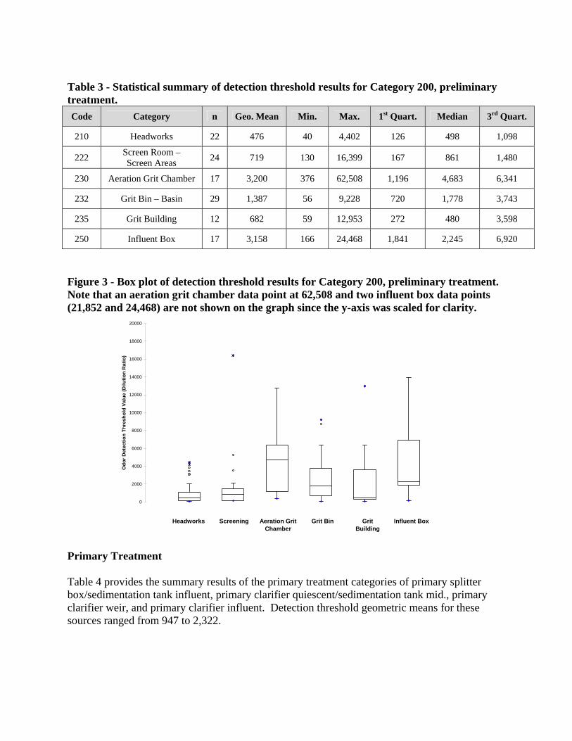
Table 3 - Statistical summary of detection threshold results for Category 200, preliminary treatment. Code Category n Geo. Mean Min. Max. 1st Quart. Median 3rd Quart.

210 Headworks 22 476 40 4,402 126 498 1,098

222 Screen Room – Screen Areas 24 719 130 16,399 167 861 1,480

230 Aeration Grit Chamber 17 3,200 376 62,508 1,196 4,683 6,341

232 Grit Bin – Basin 29 1,387 56 9,228 720 1,778 3,743

235 Grit Building 12 682 59 12,953 272 480 3,598

250 Influent Box 17 3,158 166 24,468 1,841 2,245 6,920

Figure 3 - Box plot of detection threshold results for Category 200, preliminary treatment. Note that an aeration grit chamber data point at 62,508 and two influent box data points (21,852 and 24,468) are not shown on the graph since the y-axis was scaled for clarity.

0

2000

4000

6000

8000

10000

12000

14000

16000

18000

20000

Odo

r Det

ectio

n Th

resh

old

Valu

e (D

ilutio

n R

atio

)

Headworks Screening Aeration GritChamber

Grit Bin Grit Building

Influent Box

Primary Treatment Table 4 provides the summary results of the primary treatment categories of primary splitter box/sedimentation tank influent, primary clarifier quiescent/sedimentation tank mid., primary clarifier weir, and primary clarifier influent. Detection threshold geometric means for these sources ranged from 947 to 2,322.

Table 4 - Statistical summary of detection threshold results for Category 300, primary treatment. Code Category n Geo. Mean Min. Max. 1st Quart. Median 3rd Quart.

320 Primary Splitter Box / Sed. Tank Influent 25 2,552 227 69,365 1,052 2,741 5,628

322 Primary Clarifier Quies. / Sed. Tank Mid. 69 947 12 20,088 436 1,277 2,153

324 Primary Clarifier Weir 32 2,322 115 12,387 2,262 3,166 5,363

326 Primary Clarifier Effluent 50 2,959 224 31,162 1,982 2,911 4,884

Figure 4 presents the box plots for the primary treatment sources. The primary clarifier quiescent/sedimentation tank mid. has the lowest median detection threshold, while the other three sources had similar medians, which had a small range from 2,741 to 3,166. Figure 4 - Box plot of detection threshold results for Category 300, primary treatment. Note that a splitter box data point at 69,365, a clarifier quiescent data point at 20,088, and two clarifier effluent data points (21,272 and 31,162) are not shown on the graph since the y-axis was scaled for clarity.

0

2000

4000

6000

8000

10000

12000

14000

16000

18000

20000

Odo

r Det

ectio

n Th

resh

old

Valu

e (D

ilutio

n R

atio

)

Splitter Box /Sed. Tank Influent

Clarifier Quiesent /Sed. Tank Mid.

Clarifier Weir Clarifier Effluent

Biological Treatment Biological treatment samples evaluated include the trickling filter, aeration basin, intermediate clarifier weir, and final clarifier. Over 100 aeration basin samples were identified. The detection threshold geometric means ranged from a low of 96 for the final clarifier to 1,006 for the trickling filter.

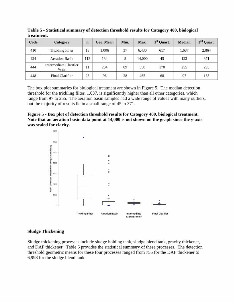
Table 5 - Statistical summary of detection threshold results for Category 400, biological treatment. Code Category n Geo. Mean Min. Max. 1st Quart. Median 3rd Quart.

410 Trickling Filter 18 1,006 37 6,430 617 1,637 2,864

424 Aeration Basin 113 134 8 14,000 45 122 371

444 Intermediate Clarifier Weir 11 234 89 550 178 255 295

448 Final Clarifier 25 96 28 465 68 97 135

The box plot summaries for biological treatment are shown in Figure 5. The median detection threshold for the trickling filter, 1,637, is significantly higher than all other categories, which range from 97 to 255. The aeration basin samples had a wide range of values with many outliers, but the majority of results lie in a small range of 45 to 371. Figure 5 - Box plot of detection threshold results for Category 400, biological treatment. Note that an aeration basin data point at 14,000 is not shown on the graph since the y-axis was scaled for clarity.

0

1000

2000

3000

4000

5000

6000

7000

Odo

r Det

ectio

n Th

resh

old

Valu

e (D

ilutio

n R

atio

)

Trickling Filter Aeration Basin Intermediate Clarifier Weir

Final Clarifier

Sludge Thickening Sludge thickening processes include sludge holding tank, sludge blend tank, gravity thickener, and DAF thickener. Table 6 provides the statistical summary of these processes. The detection threshold geometric means for these four processes ranged from 755 for the DAF thickener to 6,998 for the sludge blend tank.

Table 6 - Statistical summary of detection threshold results for Category 500, sludge thickening. Code Category n Geo. Mean Min. Max. 1st Quart. Median 3rd Quart.

530 Sludge Holding Tank 39 2,571 79 38,360 1,135 3,344 7,237

535 Sludge Blend Tank 17 6,998 1,866 19,578 4,399 6,907 13,129

540 Gravity Thickener 33 868 49 5,311 333 1,119 2,953

550 DAF Thickener 22 755 29 6,113 303 653 3,922

Figure 6 displays the box plots for these sludge thickening processes. The sludge blend tank had the highest median detection threshold, 6,907, and the widest spread of results with the 1st quartile at 4,399 and 3rd quartile at 13,128. The sludge holding tank and sludge blend tank had the highest maximum detection threshold values of 19,578 and 38,360, respectively. Figure 6 - Box plot of detection threshold results for Category 500, sludge thickening. Note that three sludge holding tank data points (28,943, 29,160, and 38,360) are not shown on the graph since the y-axis was scaled for clarity.

0

2000

4000

6000

8000

10000

12000

14000

16000

18000

20000

Odo

r Det

ectio

n Th

resh

old

Valu

e (D

ilutio

n R

atio

)

Sludge Holding Tank

Sludge Blend Tank Gravity Thickener DAF Thickener

Digesters Digester sources were placed into two categories, digester (anaerobic) vent with 14 samples and aerobic digester with 10 samples. Table 7 contains the summary statistics for these sources. The detection threshold geometric mean is 1,471 for the digester vent and 279 for the aerobic digester.

Table 7- Statistical summary of detection threshold results for Category 600, digesters. Code Category n Geo. Mean Min. Max. 1st Quart. Median 3rd Quart.

620 Digester Vent 14 1,471 77 11,473 456 2,385 5,288

630 Aerobic Digester 10 279 22 5,704 73 236 747

Figure 7 displays the box plots for these two categories. The digester vent samples had a wider range of results with the value for the 25th percentile (1st quartile) at 456 and the value for the 75th percentile (3rd quartile) at 5,288. The maximum value for the aerobic digester, excluding outliers, is lower than the median value for the digester vent. Figure 7 - Box plot of detection threshold results for Category 600, digesters.

0

2000

4000

6000

8000

10000

12000

Odo

r Det

ectio

n Th

resh

old

Valu

e (D

ilutio

n R

atio

)

Digester Vent Aerobic Digester

Dewatering Five dewatering processes were identified with more than 10 records in our database. These processes included dewatering building, belt filter press, belt filter press room, centrate, and truck loading bay. Table 8 provides a summary of the detection threshold values for the dewatering processes. The geometric means of the detection threshold for the five processes only ranged from 994 to 1,703.

Table 8 - Statistical summary of detection threshold results for Category 700, dewatering. Code Category N Geo. Mean Min. Max. 1st Quart. Median 3rd Quart.

725 Dewatering Building 22 1,105 133 73,586 273 1,105 3,020

730 Belt Filter Press 10 1,703 108 10,508 1,409 2,665 3,357

735 Belt Filter Press Room 15 994 48 3,568 678 1,288 2,122

750 Centrate 15 1,150 298 47,255 390 588 1,920

760 Truck Loading Bay 23 1,638 76 65,613 762 2,268 3,883

The box plots of dewatering processes are displayed in Figure 8. While the belt filter press room has the lowest geometric mean of detection threshold, 994, the centrate process has the lowest median detection threshold value of 588. While the maximum reported values were highest for dewatering building and tuck loading bay, the interquartile range of 25th to 75th percentile were vary similar with the 1st quartile values ranging from 273 to 1,409 and the 3rd quartile range from 2,122 to 3,883. Figure 8 - Box plot of detection threshold results for Category 700, dewatering. Note that a dewatering data point (73,586), a belt filter press data point (10,508), two centrate data points (12,853 and 47,255), and a truck loading bay data point (65,613) are not shown on the graph since the y-axis was scaled for clarity.

0

1000

2000

3000

4000

5000

6000

7000

8000

9000

10000

Odo

r Det

ectio

n Th

resh

old

Valu

e (D

ilutio

n R

atio

)

Dewatering Building

Belt Filter Press Belt FilterPress Room

Centrate Truck Loading Bay

Biosolids Biosolids processes identified include Biosolids and compost material. Table 9 provides the summary statistics for the Biosolids processes. Note that details of the types of compost materials and biosolids were not identified in the specific sample descriptions. The geometric mean detection threshold values are 584 for Biosolids and 707 for compost material. Table 9 - Statistical summary of detection threshold results for Category 800, biosolids. Code Category n Geo. Mean Min. Max. 1st Quart. Median 3rd Quart.

810 Biosolids 12 584 167 4,794 362 427 772

820 Compost Material 45 707 155 4,686 409 693 1,221

Figure 9 presents the box plots for the biosolids processes. The two processes have similar statistical values with a median threshold value of 427 for biosolids and 693 for compost material. The 45 samples identified as compost materials had a wider range of threshold values compared to the 12 biosolids samples. Figure 9 - Box plot detection threshold results for Category 800, biosolids.

0

500

1000

1500

2000

2500

3000

3500

4000

4500

5000

Odo

r Det

ectio

n Th

resh

old

Valu

e (D

ilutio

n R

atio

)

Biosolids Compost Material

Odor Control Systems Four odor control systems were identified among the WWTP process samples including carbon, chemical scrubbers, bio-scrubbers, and biofilters. Since the sources for control system inlets vary greatly, the statistical summary would not be representative of anything; therefore, only control system outlet samples were reviewed. Of all sample sets evaluated, the scrubber and biofilter outlets were the two largest samples with 185 and 140 data points, respectively. Odor

control systems was the main category with the highest overall number of samples. Table 10 provides a summary of the statistics from this sample set. Bio-scrubber outlets had the highest detection threshold geometric mean with a value of 1,843. The biofilter outlets had the lowest detection threshold geometric mean of 198; however, carbon system outlets were very similar with a geometric mean of 202. Table 10 - Statistical summary of detection thrreshold results for Category 900, odor control systems. Code Category n Geo. Mean Min. Max. 1st Quart. Median 3rd Quart.

910 Carbon Outlets 92 202 19 10,773 55 99 774

930 Scrubber Outlets 185 444 5 14,855 163 357 1,416

940 Bio-Scrubber Outlets 23 1,843 236 6,363 1,104 2,524 3,232

950 Biofilter Outlets 140 198 14 30,412 61 165 470

Figure 10 displays the box plots for the four types of odor control system outlets. The median detection threshold value of 99 for carbon systems was the lowest of all types. The 75th percentile of carbon and biofilter system outlets are lower than the 75th percentile of the chemical scrubber outlets and below the median of the bio-scrubber outlets. Figure 10 - Box plot detection threshold results for Category 900, odor control systems. Note that three carbon system data points (9,865, 10,047, and 10,773), a chemical scrubber data point (14,855), and four biofilter data points (9,188, 10,338, 16,680, and 30,412) are not shown on the graph since the y-axis was scaled for clarity.

0

1000

2000

3000

4000

5000

6000

7000

Odo

r Det

ectio

n Th

resh

old

Valu

e (D

ilutio

n R

atio

)

Carbon Chemical Scrubber Bio-Scrubber Biofilter

Hydrogen Sulfide Odor Threshold Correlation From 1999-2007, there were 3,584 WWTP odor samples submitted to St. Croix Sensory with hydrogen sulfide concentration information provided on Chain of Custody documentation. The hydrogen sulfide concentrations were not measured or otherwise confirmed by St. Croix Sensory. There were 2,373 samples with hydrogen sulfide concentration of 0.01-20ppm. These results were plotted to examine a correlation between hydrogen sulfide and odor detection threshold. Figure 11 is the plot of log detection threshold vs. log hydrogen sulfide concentration. The best fit line has an equation of Log (detection threshold) = 0.43 * Log(H2S Conc.) + 3.28 [R=0.60] Note that the x-axis intercept, x=0 or 100=1ppm, is a log detection threshold of 3.28, which is DT=103.28=1,905. This is a hydrogen sulfide detection threshold value of 0.52ppb (1,000ppb/1,905), a value generally in agreement with published odor threshold data. Figure 11 - Relationship of detection threshold and hydrogen sulfide concentration displayed as a log-log plot of threshold values determined for samples with reported hydrogen sulfide concentrations in the range of 10 ppb to 20ppm.

y = 0.43x + 3.28R2 = 0.36

0.0

0.5

1.0

1.5

2.0

2.5

3.0

3.5

4.0

4.5

5.0

-2.5 -2.0 -1.5 -1.0 -0.5 0.0 0.5 1.0 1.5

Log Hydrogen Sulfide Conc. (log ppm)

Log

Det

ectio

n Th

resh

old

(Log

DT)

Comparison of Olfactometer Presentation Flow Rates Over 100 samples in the database were analyzed on both the AC’SCENT International Olfactometer with a presentation flow rate of 20-LPM and an Illinois Institute of Technology Research Institute (IITRI) Olfactometer with a presentation flow rate of 0.5-LPM. Tests run on the AC’SCENT Olfactometer were conducted according the EN13725:2003 and ASTM E679-04 (Appendix X.3). Tests run on the IITRI Olfactometer were conducted according to ASTM E679-04 (Appendix X.2). A review of the samples evaluated at both presentation flow rates provided the following correlation equation for Detection Threshold (DT) values of 50-6,000 determined at 20LPM (DT’s of 5-3,000 determined at 0.5LPM): Log(DT0.5LPM) = 0.24 * [Log(DT20LPM)]2.0

The following equation can be utilized when converting from a DT at 0.5LPM to DT at 20LPM: Log(DT20LPM) = 2.04 * [Log(DT0.5LPM)]0.5 DISCUSSION AND CONCLUSIONS A review of odor detection threshold results from over 1,000 samples of various WWTP process sources provides a statistical summary for determining emission factors for comparison to measurements made during actual testing or for estimating emissions from plants under development. When interpreting the results presented in this paper it is important to note that all data points are based on samples received by a commercial laboratory without any qualification of the samples. For example, in the review of carbon system outlets, some high values could be the result of samples collected from systems that were tested with the expectation that they were not performing well. Additionally, variations in values are likely the outcome of the wide range of variables related to the wastewater and related air emissions. It is also important to note that the geometric mean can be biased high due to many outlier values on the high end. It is important to not only look at the geometric mean provided in the data tables, but also the information provided by the box plots. For example, a median value that is significantly lower than the geometric mean would suggest there were several high outlier points. The following are a list of notable results from this data review of WWTP samples:

Table 11 - Summary of Detection Threshold (DT) geometric mean results for selected process categories. Code Category DT

Geo. Mean

010 Blanks 13

020 Ambient/Background 40

210 Headworks 480

222 Screen Room – Screen Areas 720

230 Aeration Grit Chamber 3,200

232 Grit Bin - Basin 1,400

235 Grit Building 680

250 Influent Box 3,200

320 Primary Splitter Box / Sed. Tank Influent 2,600

322 Primary Clarifier Quies. / Sed. Tank Mid. 950

324 Primary Clarifier Weir 2,300

326 Primary Clarifier Effluent 3,000

410 Trickling Filter 1,000

424 Aeration Basin 130

444 Intermediate Clarifier Weir 230

448 Final Clarifier 100

530 Sludge Holding Tank 2,600

535 Sludge Blend Tank 7,000

540 Gravity Thickener 870

550 DAF Thickener 760

910 Carbon Outlets 200

930 Scrubber Outlets 440

940 Bio-Scrubber Outlets 1,800

950 Biofilter Outlets 200

The review of odor detection threshold values with corresponding hydrogen sulfide concentration provides a poor overall correlation. However, the graph and resulting trendline can be used in some instances to provide a fair estimate of the expected value of one variable if the other is known. It is most important to note that for higher concentrations of hydrogen sulfide, knowing the concentration will allow you to make an estimate of order of magnitude of the detection threshold. The same is not true for low hydrogen sulfide concentration. Many samples reviewed with hydrogen sulfide concentrations less than 10ppb had detection threshold values across a wide range since other chemical odorants were also present in some samples. A review of threshold values determined at both 0.5LPM and 20LPM provides a correlation equation that can be used to take the detection threshold (DT) value from one presentation flow rate to estimate the DT value expected with another flow rate. The following equation can be used to convert threshold values in the range of 50-6,000, determined at 20LPM, to the value that would be expected at 0.5LPM: Log(DT0.5LPM) = 0.24 * [Log(DT20LPM)]2.0

While this equation will provide a reasonable estimate when needing to compare a value determined with one presentation flow rate to the expected value determined by the other flow rate. One must keep in mind the actual value could vary depending on the source and chemistry of the odorous air sample. ACKNOWLEDGEMENTS The authors would like to acknowledge the clients, staff and assessors at St. Croix Sensory, Inc. for their involvement in determination of the threshold results used for the data in this report. REFERENCES ASTM International (2004). E679-04: Standard Practice for Determination of Odor and Taste

Threshold by a Forced-Choice Ascending Concentration Series Method of Limits. Philadelphia, PA, USA.

Committee for European Normalization (CEN) (2003). EN13725: Air Quality – Determination

of Odour Concentration by Dynamic Olfactometry, Brussels, Belgium. Water Environment Federation (2004) Control of Odors and Emissions from Waste Water

Treatment Plants, 1st ed.; Manual of Practice No. 25; Alexandria, Virginia.