IFT-UAM/CSIC-16-032

Odd viscosity in the quantum critical region of a

holographic Weyl semimetal

Karl Landsteiner1, Yan Liu2 and Ya-Wen Sun3

Instituto de Fısica Teorica UAM/CSIC, C/ Nicolas Cabrera 13-15,

Universidad Autonoma de Madrid, Cantoblanco, 28049 Madrid, Spain

Abstract

We study odd viscosity in a holographic model of a Weyl semimetal. The model is

characterised by a quantum phase transition from a topological semimetal to a trivial

semimetal state. Since the model is axisymmetric in three spatial dimensions there

are two independent odd viscosities. Both odd viscosity coefficients are non-vanishing

in the quantum critical region and non-zero only due to the mixed axial gravitational

anomaly. It is therefore a novel example in which the mixed axial gravitational anomaly

gives rise to a transport coefficient at first order in derivatives at finite temperature.

We also compute anisotropic shear viscosities and show that one of them violates

the KSS bound. In the quantum critical region, the physics of viscosities as well as

conductivities is governed by the quantum critical point.

1Email: karl.landsteiner@uam.es2Email: yanliu.th@gmail.com3Email: yawen.sun@csic.es

arX

iv:1

604.

0134

6v1

[he

p-th

] 5

Apr

201

6

Introduction.– One of the most surprising outcomes of string theory is the application

of the AdS/CFT correspondence to the physics of strongly interacting quantum many-body

systems [1]. The need to develop models that allow to address the question of real-time

transport in strongly interacting quantum fluids has arisen from experiments in completely

different areas of physics: in the quark gluon plasma generated in heavy ion collisions, the

collective behavior of ultra-cold atoms, the strange metal phase of the high-Tc superconduc-

tors and most recently the hydrodynamic electronic flow observed in Graphene and similar

materials [2–5].

Graphene is a “Dirac” semimetal in which the electrons are well described by the Dirac

equation. The motion of electrons in Graphene is however restricted to two spatial dimen-

sions. In the last few years new materials whose electronics is described by the Dirac or Weyl

equation in three spatial dimensions have been demonstrated [6–8]. These Weyl semimetals

have a plethora of exciting and exotic transport properties related to the chiral anomaly of

three dimensional relativistic fermions.

As in Graphene the electron fluid within a Weyl semimetal might as well be strongly

interacting due to the smallness of the Fermi velocity compared to the speed of light. It

seems therefore natural to ask if holography can be applied to such systems as well. In

this case holography should play a similar important role for the understanding of quantum

transport of Weyl semimetals as it already does in the theory of the quark gluon plasma [9].

In particular we ask the question if one can learn something new from holographic models

utilizing universal properties of these materials such as the (effective) presence of chiral

anomalies. We will address this question and answer it to the affirmative.

Holographic Weyl semimetal.– Recently a holographic model of a Weyl semimetal has

been developed in [10, 11]. Let us briefly review the most salient feature of this model. Its

action is given by

S =

∫d5x√−g[

1

2κ2

(R +

12

L2

)− 1

4e2F2 − 1

4e2F 2 − (DµΦ)∗(DµΦ)− V (Φ) (0.1)

+ εµνρστAµ

(α

3

(FνρFστ + 3FνρFστ

)+ ζRβ

δνρRδβστ

)],

with Fµν = ∂µVν − ∂νVµ, Fµν = ∂µAν − ∂νAµ and DµΦ = (∂µ − iqAµ)Φ. The holographic

dictionary determines the field content of the model. The metric encodes the dynamics of

the energy momentum tensor. There are two gauge fields. The first one, denoted by Vµ, is

dual to a conserved vector U(1) current that can be identified with the electric current. The

second one, Aµ, is an axial gauge field. It couples to the complex scalar field Φ via an axial

covariant derivative. The axial current suffers also from the axial anomaly which has three

parts: one is the electro-magnetic contribution to the axial anomaly, the second one is the

purely axial U(1)3A anomaly and the third one is the gravitational contribution to the axial

anomaly (i.e. mixed axial gravitational anomaly). These three anomalies are represented

by the Chern-Simons terms in the action (0.1). The scalar field potential is chosen to be

1

V (Φ) = m2|Φ|2 + λ2|Φ|4. The mass determines the dimension of the operator dual to Φ and

we chose it to be m2L2 = −3.4 The boundary value of the scalar field is dual to a mass

deformation in the field theory.

In [11] the boundary conditions5

limr→∞

rΦ = M , limr→∞

Az = b (0.2)

together with asymptotic AdS behaviour of the metric were considered. Choosing further-

more the scalar field charge q = 1 and the scalar self coupling λ = 1/10 it was found that

the model undergoes a quantum phase transition as function of the dimensionless parameter

M/b. Note that the mixed axial gravitational anomaly is included in the holographic Weyl

semimetal model (0.1) while it does not play any role in all the discussions of [11], including

the phase transition and electric conductivities. This model can be understood as a gravity

analogue of the Lorentz breaking Dirac system with Lagrangian[γµ(i∂µ − evµ − γ5bδ

zµ) +M

]Ψ = 0 . (0.3)

This Lorentz breaking Dirac system has been used as a model for Weyl semimetals before

in e.g. [14–17].

At zero temperature for M/b < 0.744 the scalar field vanishes in the IR towards r = 0

whereas the axial gauge field takes a non-vanishing value Az|r=0 = beff . In this regime

the model has a non-vanishing anomalous Hall conductivity given by σAHE = 8αbeff . For

M/b > 0.744 the axial gauge field vanishes in the IR whereas the scalar field takes a finite

value that is determined by the minimum of the potential V ′(Φ) = 0. In this phase the

anomalous Hall conductivity vanishes. The model undergoes therefore a topological quantum

phase transition between a topological state of semimetal state with non-vanishing anomalous

Hall conductivity and a trivial semimetal state with vanishing anomalous Hall conductivity.

There is an emergent Lifshitz symmetry at the critical point M/b ' 0.744 and it governs

the quantum critical physics at finite temperature [18]. Moreover, at low temperature the

ohmic DC conductivity scales as σxx = σyy = cT and σzz = cT except near the quantum

critical regime [11] as can be expected from a three dimensional Weyl- or Dirac semimetal.

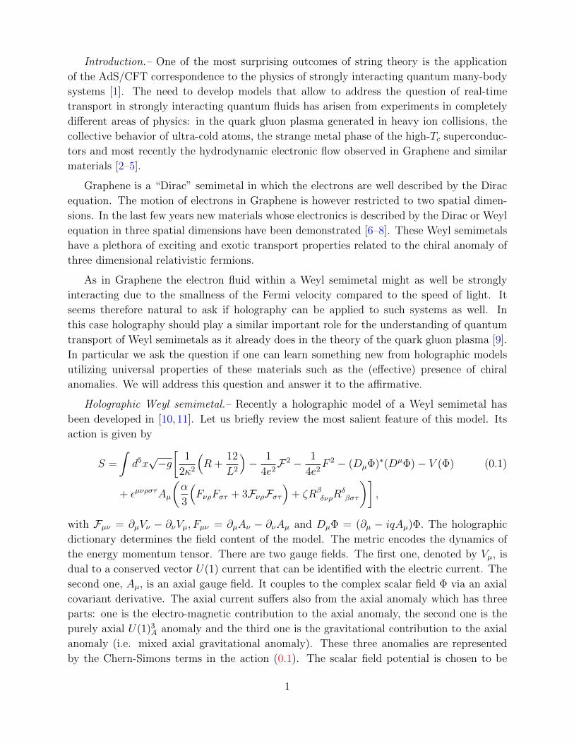
A cartoon illustration for our model (0.1) is shown in Fig. 1.

Viscosities.– A necessary ingredient for the presence of odd viscosity is broken time

reversal symmetry [19–22]. This is in principle provided by the axial gauge field background

b. We note however that this is a UV parameter and we could expect that the viscosity

is determined rather by the IR properties, similar to the anomalous Hall conductivity. It

follows then that in the topological trivial phase in which time reversal symmetry is restored

at the endpoint of the holographic RG flow beff = 0 we should not expect substantial odd

4Here L is the scale of the AdS space. In the following we set 2κ2 = e2 = L = 1.5The same setup with different boundary conditions was also used in [12, 13] to realize axial charge

dissipations in the study of negative magnetoresistivity of the holographic Dirac semimetal.

2

0 (M/b)c M/b

T

Weyl

semimetal

quantum

critical

topologically

trivial semimetal

Figure 1: The cartoon picture for the holographic Weyl semimetal model in the coupling constant

(M/b) - temperature (T ) plane. At zero temperature a topological quantum phase transition occurs

at the critical value (M/b)c. At finite temperature the dashed line is a smooth crossover and in the

quantum critical regime the physics is governed by the quantum critical behaviour.

viscosity. On the other hand one can also argue that odd viscosity should be absent in the

topological phase at zero temperature. At weak coupling the argument goes as follows: the

low energy effective model describing a Weyl semimetal is

S =

∫d4xΨ(iγµ∂µ − eγµvµ − γ5γzbeff)Ψ . (0.4)

By a field redefinition the parameter beff can be removed from the action at the cost of

introducing the anomalous effective term

Γanom =

∫d4x√−γ(beff · z)εµνρλ

(αFµνFρλ +

α

3FµνFρλ + ζRα

βµνRβαρλ

). (0.5)

The anomaly (0.5) encodes the response at zero temperature and shows that there is Hall

conductivity but no odd (Hall) viscosity. Rather the gravitational response is third order in

derivatives as the Riemann curvature is second order in derivatives on the metric. We note

that at finite temperature this derivative counting is not necessarily correct anymore. A well

known example for this is the contribution of the mixed axial gravitational anomaly to the

chiral vortical effect [23,24]. As we will show now in our holographic model the gravitational

contribution to the axial anomaly is also able to induce odd viscosity (a first order effect in

derivatives) once temperature is switched on.

In an axisymmetric system characterised by a time reversal breaking vector such as ~b

there are seven6 independent viscosities [21] in which there are two independent odd viscosity

6In a 3+1 dimensional axisymmetry system with a time reversal breaking vector, there are seven compo-

nents in the viscosity tensor, including three shear viscosities, two odd viscosities and two bulk viscosities.

Besides the four components below, there are another two bulk viscosities and one shear viscosity which

come from the spin zero components of xx+ yy and zz, which we do not consider in this paper.

3

tensor components. We can define the viscosities via the Kubo formula

ηij,kl = limω→0

1

ωIm[GRij,kl(ω, 0)

], (0.6)

with the retarded Green’s function of the energy momentum tensor

GRij,kl(ω, 0) = −

∫dtd3xeiωtθ(t)〈[Tij(t, ~x), Tkl(0, 0)]〉 . (0.7)

Since we chose our coordinates such that ~b = bez is a convenient basis, for the two shear

viscosities which are related to the symmetric part of the retarded Green’s function under

the exchange of (ij)↔ (kl)

η‖ = ηxz,xz = ηyz,yz , η⊥ = ηxy,xy = ηT,T (0.8)

and for the two odd components of viscosity which are related to the antisymmetric part

ηH‖ = −ηxz,yz = ηyz,xz , ηH⊥ = ηxy,T = −ηT,xy (0.9)

where T denotes the index combination xx − yy. We note that ηH⊥ can be understood as

Hall viscosity in the plane orthogonal to ~b whereas ηH‖ is specific to axisymmetric three

dimensional systems. The later has been shown to arise also via the coupling of elastic

gauge fields to the electron gas in Weyl semimetals [25]. In that case the odd or Hall

viscosity is best thought of as a property of the phonon gas arising via the electron-phonon

Chern-Simons interactions. This effective Hall viscosity is related to the underlying Hall

conductivity of the electron gas and arises from the electronic point of view as an axial Hall

conductivity. In contrast here we will be dealing with Hall or odd viscosity as an intrinsic

property of the strongly coupled electron fluid. Hall viscosity arising from gravitational

θ−terms in holographic models dual to 2 + 1 dimensional field theories has been studied

before in e.g. [26–32]. In contrast our system is dual to a 3 + 1 dimensional theory with a

mixed axial gravitational anomaly represented by the five dimensional gravitational Chern-

Simons term in (0.1).

We use the following ansatz for the background at finite temperature

ds2 = −udt2 +dr2

u+ f(dx2 + dy2) + hdz2

A = Azdz , Φ = φ (0.10)

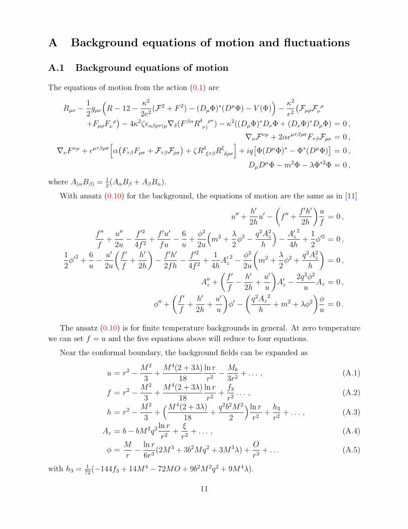
with the fields u, f, h, Az, φ real functions of r. Background equations of motion are sum-

marised in appendix A. It turns out that they are independent of the Chern-Simons couplings

α and ζ and the numerical solutions have been studied in [11]. At finite temperature there

is a horizon at a finite value r = r0. The entropy density is given by the area element of the

horizon s = 4πf√h∣∣r=r0

. In order to probe the interesting non-trivial IR physics and relate

our findings to possible applications to physical Weyl semimetals we should work at small

4

temperatures. At higher temperatures it is rather the UV-completion of the model that is

probed.

Longitudinal viscosity: In order to compute the viscosities we switch on the following

perturbations: δgiz = hiz(r)e−iωt , δAi = ai(r)e

−iωt for i ∈ {x, y}. They form the complex

combination h± = hxz ± ihyz and a± = ax ± iay. The resulting equations of motion are

rather cumbersome to treat, but after a lengthy but straightforward analysis the solutions

to lowest order in ω can be written as (see appendix B for details)

h± = r2 − M2

3+M4(2 + 3λ)

18

ln r

r2+

1

r2

[f3 +

ω

4

([if 2

√h± 4ζ

q2Azφ2f 2

h

]∣∣∣r=r0

)]+ . . . (0.11)

near the conformal boundary. Here f3 is the coefficient of the 1/r2 term in the asymptotic

expansion of metric function (A.2). From the first order term in ω we can read off the

following two viscosity coefficients,

dissipative viscosity: η‖ = ηxz,xz = ηyz,yz =f 2

√h

∣∣∣∣r=r0

(0.12)

dissipationless odd viscosity: ηH‖ = ηyz,xz = −ηxz,yz = 4ζq2Azφ

2f 2

h

∣∣∣∣r=r0

. (0.13)

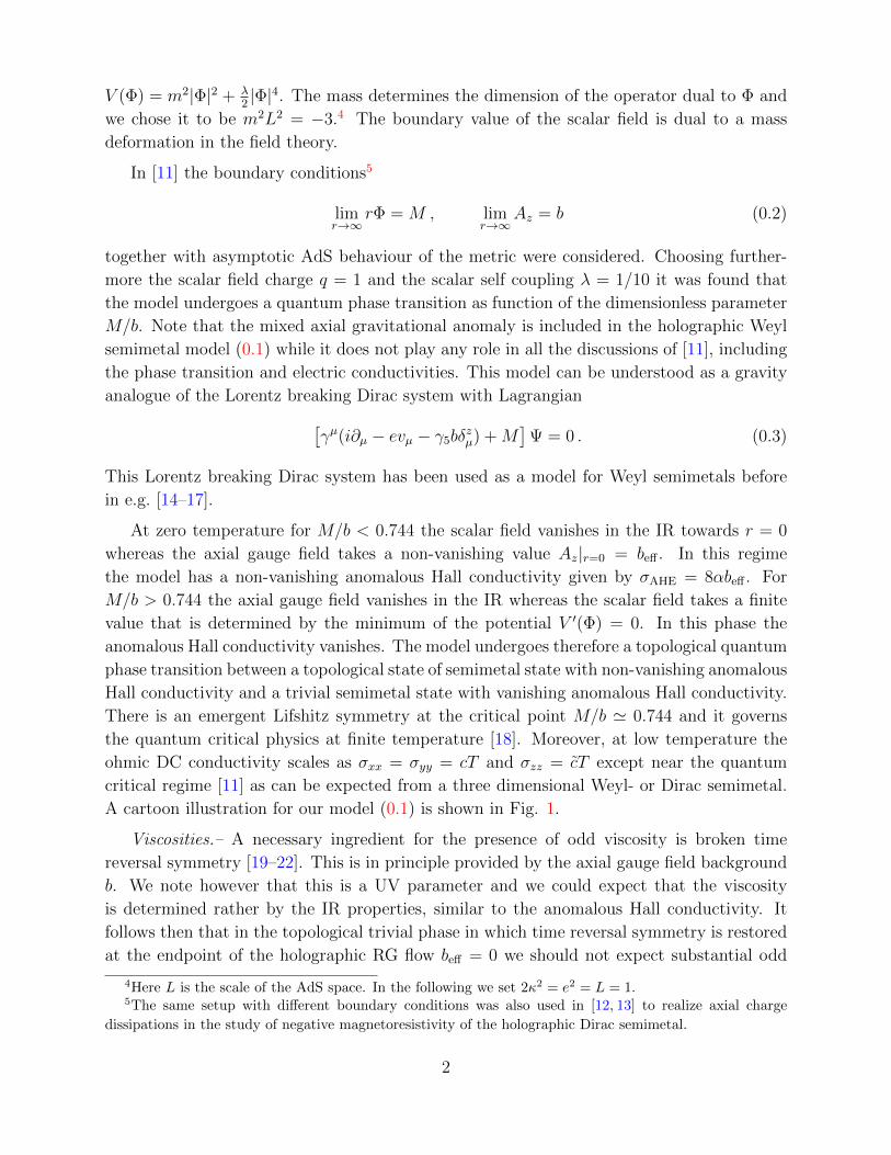
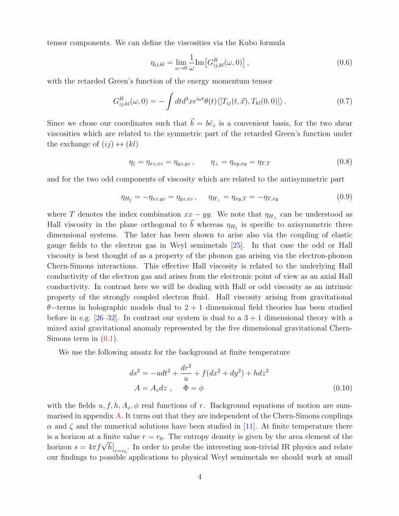
The dissipative viscosity is a form of shear viscosity and it is interesting to express it nor-

malized to the entropy densityη‖s

= f4πh|r=r0 . As can be seen from Fig. 2 the shear viscosity

drops significantly below the standard result of KSS bound [33]. In view of the various

results of violation of the KSS bound in anisotropic theories [34, 35] this is not unexpected.

Still it is very interesting to note that the shear viscosity reaches a minimum in the quantum

critical region of M/b ≈ 0.744 as shown in Fig. 2.

T/b=0.05

T/b=0.04

T/b=0.03

��� ��� ��� ��� ��� ��� ������

���

���

���

���

���

�

�

�πη∥�

Figure 2: The longitudinal shear viscosity over entropy density 4πη‖s as a function of M/b at

different temperatures.

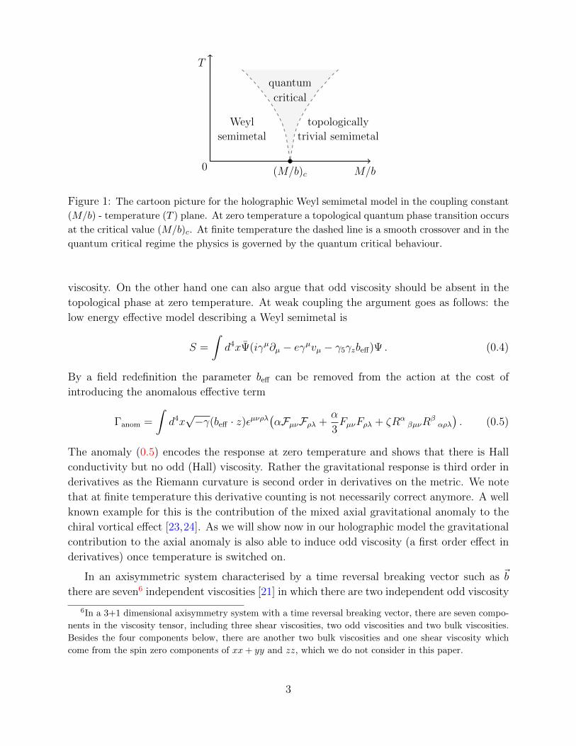
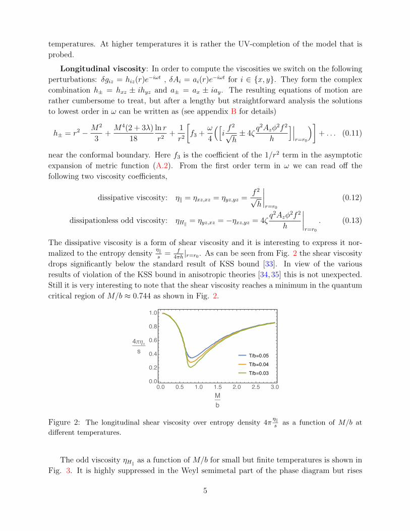
The odd viscosity ηH‖ as a function of M/b for small but finite temperatures is shown in

Fig. 3. It is highly suppressed in the Weyl semimetal part of the phase diagram but rises

5

steeply as the quantum critical region around M/b ' 0.744 is entered. It peaks roughly

at the critical value and then falls off in a somewhat slower fashion as M/b increases. The

extreme M/b→∞ limit can be reached by setting b = 0 keeping M finite. In this case the

field Az is simply zero along the holographic RG flow and from (0.13) it follows that the odd

viscosity vanishes again in this limit.

T/b=0.05

T/b=0.04

T/b=0.03

��� ��� ��� ��� ��� ��� ����

�

��

��

��

��

�

�

η�∥

��

Figure 3: Odd viscosity ηH‖ as a function of M/b at different temperatures.

Transverse viscosity: We switch on the perturbations δgxx − δgyy = 2hL(r)e−iωt ,

δgxy = hxy(r)e−iωt and form the complex combination H± = hL ± ihxy. Expanding to first

order in ω we find (see appendix C for details)

H± = r2 − M2

3+M4(2 + 3λ)

18

ln r

r2+

1

r2

(f3 +

ω

4

([if√h± 8ζq2φ2fAz

]∣∣∣r=r0

))+ . . .

(0.14)

near the conformal boundary. Using the holographic dictionary we can read off the viscosities

from the terms at first order in ω at order 1/r2 in the large r expansion. The dissipative

viscosity is

η⊥ = f√h∣∣∣r=r0

. (0.15)

We note that in this case the KSS bound is exactly obeyed η⊥/s = 1/4π. The non-dissipative

odd viscosity is

ηH⊥ = 8ζq2φ2fAz

∣∣∣r=r0

. (0.16)

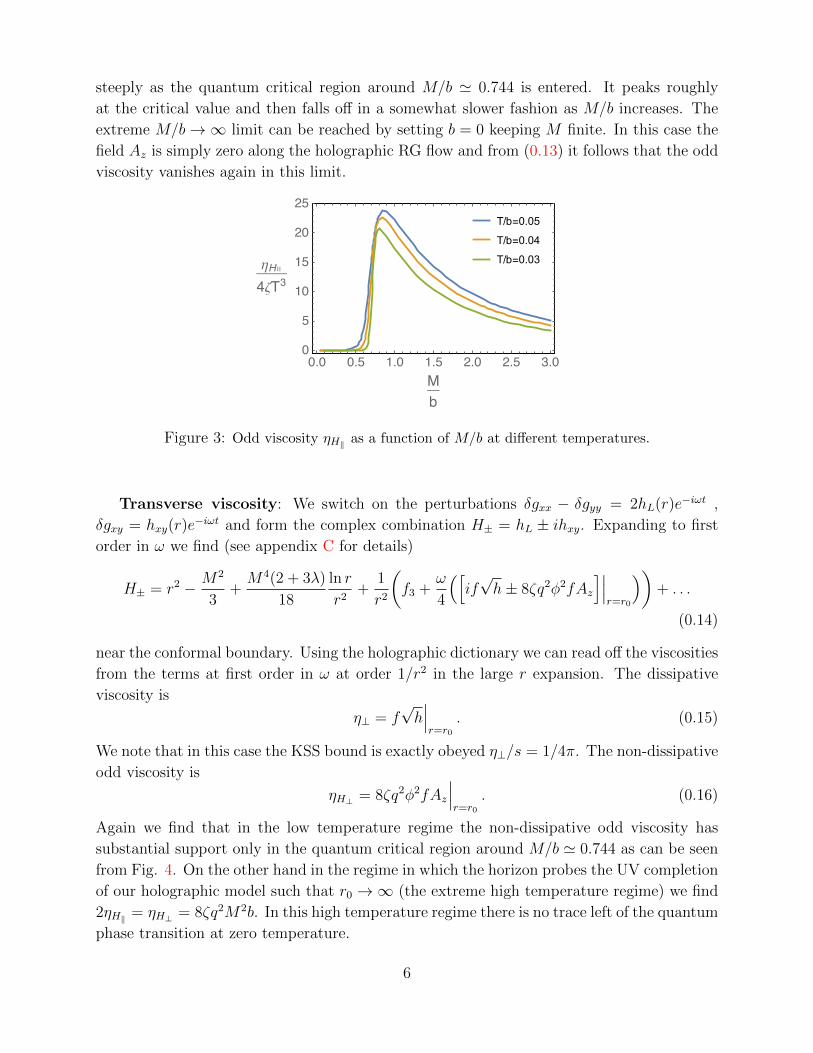
Again we find that in the low temperature regime the non-dissipative odd viscosity has

substantial support only in the quantum critical region around M/b ' 0.744 as can be seen

from Fig. 4. On the other hand in the regime in which the horizon probes the UV completion

of our holographic model such that r0 →∞ (the extreme high temperature regime) we find

2ηH‖ = ηH⊥ = 8ζq2M2b. In this high temperature regime there is no trace left of the quantum

phase transition at zero temperature.

6

T/b=0.05

T/b=0.04

T/b=0.03

��� ��� ��� ��� ��� ��� ����

��

��

��

��

���

�

�

η�⊥

��

Figure 4: Odd viscosity ηH⊥ as a function of M/b at different low temperatures.

We also note that the analytic results on the viscosities (together with our previous result

on the conductivities in [11]) allow us to obtain the non-trivial relation

η‖η⊥

=2ηH‖

ηH⊥

=σ‖σ⊥

=f

h

∣∣∣∣r=r0

(0.17)

where σ‖ = σzz = f√h

∣∣r=r0

, σ⊥ = σxx = σyy =√h∣∣r=r0

.

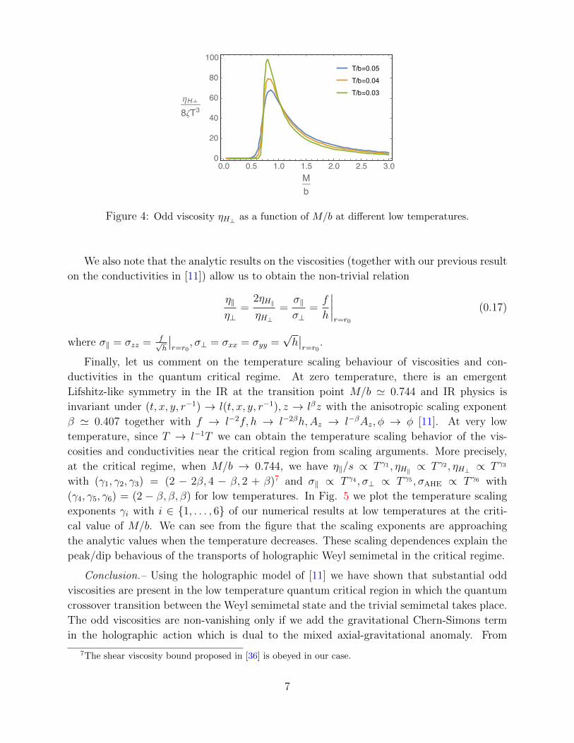
Finally, let us comment on the temperature scaling behaviour of viscosities and con-

ductivities in the quantum critical regime. At zero temperature, there is an emergent

Lifshitz-like symmetry in the IR at the transition point M/b ' 0.744 and IR physics is

invariant under (t, x, y, r−1) → l(t, x, y, r−1), z → lβz with the anisotropic scaling exponent

β ' 0.407 together with f → l−2f, h → l−2βh,Az → l−βAz, φ → φ [11]. At very low

temperature, since T → l−1T we can obtain the temperature scaling behavior of the vis-

cosities and conductivities near the critical region from scaling arguments. More precisely,

at the critical regime, when M/b → 0.744, we have η‖/s ∝ T γ1 , ηH‖ ∝ T γ2 , ηH⊥ ∝ T γ3

with (γ1, γ2, γ3) = (2 − 2β, 4 − β, 2 + β)7 and σ‖ ∝ T γ4 , σ⊥ ∝ T γ5 , σAHE ∝ T γ6 with

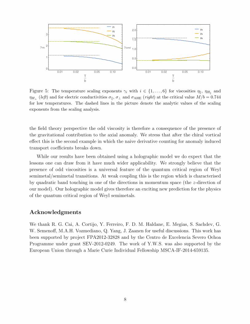
(γ4, γ5, γ6) = (2 − β, β, β) for low temperatures. In Fig. 5 we plot the temperature scaling

exponents γi with i ∈ {1, . . . , 6} of our numerical results at low temperatures at the criti-

cal value of M/b. We can see from the figure that the scaling exponents are approaching

the analytic values when the temperature decreases. These scaling dependences explain the

peak/dip behavious of the transports of holographic Weyl semimetal in the critical regime.

Conclusion.– Using the holographic model of [11] we have shown that substantial odd

viscosities are present in the low temperature quantum critical region in which the quantum

crossover transition between the Weyl semimetal state and the trivial semimetal takes place.

The odd viscosities are non-vanishing only if we add the gravitational Chern-Simons term

in the holographic action which is dual to the mixed axial-gravitational anomaly. From

7The shear viscosity bound proposed in [36] is obeyed in our case.

7

γ1

γ2

γ3

���� ���� ���� �����

�

�

�

�

�

��

γ4

γ5

γ6

���� ���� ���� ����

���

���

���

���

���

�

�

���

Figure 5: The temperature scaling exponents γi with i ∈ {1, . . . , 6} for viscosities η‖, ηH‖ and

ηH⊥ (left) and for electric conductivities σ‖, σ⊥ and σAHE (right) at the critical value M/b = 0.744

for low temperatures. The dashed lines in the picture denote the analytic values of the scaling

exponents from the scaling analysis.

the field theory perspective the odd viscosity is therefore a consequence of the presence of

the gravitational contribution to the axial anomaly. We stress that after the chiral vortical

effect this is the second example in which the naive derivative counting for anomaly induced

transport coefficients breaks down.

While our results have been obtained using a holographic model we do expect that the

lessons one can draw from it have much wider applicability. We strongly believe that the

presence of odd viscosities is a universal feature of the quantum critical region of Weyl

semimetal/semimetal transitions. At weak coupling this is the region which is characterised

by quadratic band touching in one of the directions in momentum space (the z-direction of

our model). Our holographic model gives therefore an exciting new prediction for the physics

of the quantum critical region of Weyl semimetals.

Acknowledgments

We thank R. G. Cai, A. Cortijo, Y. Ferreiro, F. D. M. Haldane, E. Megias, S. Sachdev, G.

W. Semenoff, M.A.H. Vozmediano, Q. Yang, J. Zaanen for useful discussions. This work has

been supported by project FPA2012-32828 and by the Centro de Excelencia Severo Ochoa

Programme under grant SEV-2012-0249. The work of Y.W.S. was also supported by the

European Union through a Marie Curie Individual Fellowship MSCA-IF-2014-659135.

8

References

[1] J. Zaanen, Y. W. Sun, Y. Liu and K. Schalm, “Holographic Duality in Condensed Mat-

ter Physics,” Cambridge University Press, 2015.

M. Ammon and J. Erdmenger, “Gauge/Gravity Duality: Foundations and Applica-

tions,” Cambridge University Press, 2015.

H. Nastase,“Introduction to the AdS/CFT Correspondence,” Cambridge University

Press, 2015.

[2] J. Zaanen, Science 351, 1026-1027 (2016).

[3] D. A. Bandurin, I. Torre, R. K. Kumar, M. B. Shalom, A. Tomadin, A. Principi, G.

H. Auton, E. Khestanova, K. S. Novoselov, I. V. Grigorieva, L. A. Ponomarenko, A. K.

Geim, M. Polini, Science 351, 1055-1058 (2016), [arXiv:1509.04165 [cond-mat.str-el]].

[4] J. Crossno, J. K. Shi, K. Wang, X. Liu, A. Harzheim, A. Lucas, S. Sachdev, P. Kim,

T. Taniguchi, K. Watanabe, T. A. Ohki, K. C. Fong, Science 351, 1058-1061 (2016),

[arXiv:1509.04713 [cond-mat.mes-hall]].

[5] P. J. W. Moll, P. Kushwaha, N. Nandi, B. Schmidt, A. P. Mackenzie, Science 351,

1061-1064 (2016), [arXiv:1509.05691 [cond-mat.str-el]].

[6] A. Vishwanat, Physics 8, 84.

[7] O. Vafek and A. Vishwanat, Annual Review of Condensed Matter Physics, Vol. 5: 83-

112, [arXiv:1306.2272 [cond-mat.str-el]].

[8] P. Hosur and X. Qi, Comptes Rendus Physique 14, 857 (2013), [arXiv:1309.4464 [cond-

mat.str-el]].

[9] J. Casalderrey-Solana, H. Liu, D. Mateos, K. Rajagopal and U. A. Wiedemann,

arXiv:1101.0618 [hep-th].

[10] K. Landsteiner and Y. Liu, Phys. Lett. B 753, 453 (2016), [arXiv:1505.04772 [hep-th]].

[11] K. Landsteiner, Y. Liu and Y. W. Sun, Phys. Rev. Lett. 116 (2016) no.8, 081602,

[arXiv:1511.05505 [hep-th]].

[12] A. Jimenez-Alba, K. Landsteiner, Y. Liu and Y. W. Sun, JHEP 1507, 117 (2015)

[arXiv:1504.06566 [hep-th]].

[13] Y. W. Sun and Q. Yang, arXiv:1603.02624 [hep-th].

[14] A. A. Burkov and L. Balents, Phys. Rev. Lett. 107, 127205, [arXiv:1105.5138 [cond-

mat.mes-hall]].

[15] A. G. Grushin, Phys. Rev. D 86 (2012) 045001, [arXiv:1205.3722 [hep-th]].

[16] A. A. Zyuzin and A. A. Burkov, Phys. Rev. B 86 (2012) 115133, [arXiv:1206.1868

[cond-mat.mes-hall]].

[17] G. E. Volovik, arXiv:1604.00849 [cond-mat.other].

9

[18] S. Sachdev, “Quantum phase transitions,” Cambridge University Press, 1999.

[19] J. E. Avron, R. Seiler, and P. G. Zograf, Phys. Rev. Lett. 75, 697, [arXiv:cond-

mat/9502011]

[20] C. Hoyos, Int. J. Mod. Phys. B 28 (2014) 1430007, [arXiv:1403.4739 [cond-mat.mes-

hall]].

[21] E. M. Lifschityz and L. P. Pitaevski, “Physical Kinetics,” Butterworth-Heinemann,

1981.

[22] F. M. Haehl, R. Loganayagam and M. Rangamani, JHEP 1505, 060 (2015),

[arXiv:1502.00636 [hep-th]].

[23] K. Landsteiner, E. Megias and F. Pena-Benitez, Phys. Rev. Lett. 107 (2011) 021601,

[arXiv:1103.5006 [hep-ph]].

[24] K. Landsteiner, E. Megias, L. Melgar and F. Pena-Benitez, JHEP 1109 (2011) 121,

[arXiv:1107.0368 [hep-th]].

[25] A. Cortijo, Y. Ferreiros, K. Landsteiner and M. A. H. Vozmediano, Phys. Rev. Lett.

115, 177202 (2015), [arXiv:1603.02674 [cond-mat.mes-hall]].

[26] O. Saremi and D. T. Son, JHEP 1204 (2012) 091, [arXiv:1103.4851 [hep-th]].

[27] J. W. Chen, S. H. Dai, N. E. Lee and D. Maity, JHEP 1209, 096 (2012),

[arXiv:1206.0850 [hep-th]].

[28] R. G. Cai, T. J. Li, Y. H. Qi and Y. L. Zhang, Phys. Rev. D 86, 086008 (2012),

[arXiv:1208.0658 [hep-th]].

[29] D. C. Zou and B. Wang, Phys. Rev. D 89, no. 6, 064036 (2014), [arXiv:1306.5486

[hep-th]].

[30] H. Liu, H. Ooguri and B. Stoica, Phys. Rev. D 90 (2014) no.8, 086007, [arXiv:1403.6047

[hep-th]].

[31] W. Fischler and S. Kundu, arXiv:1512.01238 [hep-th].

[32] T. Y. Zhao and T. Wang, arXiv:1512.01919 [gr-qc].

[33] P. Kovtun, D. T. Son and A. O. Starinets, Phys. Rev. Lett. 94 (2005) 111601, [hep-

th/0405231].

[34] A. Rebhan and D. Steineder, Phys. Rev. Lett. 108, 021601 (2012), [arXiv:1110.6825

[hep-th]].

[35] S. Jain, N. Kundu, K. Sen, A. Sinha and S. P. Trivedi, JHEP 1501, 005 (2015),

[arXiv:1406.4874 [hep-th]].

[36] S. A. Hartnoll, D. M. Ramirez and J. E. Santos, JHEP 1603, 170 (2016)

[arXiv:1601.02757 [hep-th]].

10

A Background equations of motion and fluctuations

A.1 Background equations of motion

The equations of motion from the action (0.1) are

Rµν −1

2gµν

(R− 12− κ2

2e2(F2 + F 2)− (DµΦ)∗(DµΦ)− V (Φ)

)− κ2

e2

(FµρF ρ

ν

+FµρFρν

)− 4κ2ζεαβρτ(µ∇δ(F

βαRδ ρτν) )− κ2((DµΦ)∗DνΦ + (DνΦ)∗DµΦ) = 0 ,

∇νFνµ + 2αεµτβρσFτβFρσ = 0 ,

∇νFνµ + εµτβρσ

[α(FτβFρσ + FτβFρσ

)+ ζRδ

ξτβRξδρσ

]+ iq

[Φ(DµΦ)∗ − Φ∗(DµΦ)

]= 0 ,

DµDµΦ−m2Φ− λΦ∗2Φ = 0 ,

where A(αBβ) = 12(AαBβ + AβBα).

With ansatz (0.10) for the background, the equations of motion are the same as in [11]

u′′ +h′

2hu′ −

(f ′′ +

f ′h′

2h

)u

f= 0 ,

f ′′

f+u′′

2u− f ′2

4f 2+f ′u′

fu− 6

u+φ2

2u

(m2 +

λ

2φ2 − q2A2

z

h

)− A′z

2

4h+

1

2φ′2 = 0 ,

1

2φ′

2+

6

u− u′

2u

(f ′

f+h′

2h

)− f ′h′

2fh− f ′2

4f 2+

1

4hA′z

2 − φ2

2u

(m2 +

λ

2φ2 +

q2A2z

h

)= 0 ,

A′′z +

(f ′

f− h′

2h+u′

u

)A′z −

2q2φ2

uAz = 0 ,

φ′′ +

(f ′

f+h′

2h+u′

u

)φ′ −

(q2Az

2

h+m2 + λφ2

)φ

u= 0 .

The ansatz (0.10) is for finite temperature backgrounds in general. At zero temperature

we can set f = u and the five equations above will reduce to four equations.

Near the conformal boundary, the background fields can be expanded as

u = r2 − M2

3+M4(2 + 3λ)

18

ln r

r2− Mb

3r2+ . . . , (A.1)

f = r2 − M2

3+M4(2 + 3λ)

18

ln r

r2+f3

r2. . . , (A.2)

h = r2 − M2

3+(M4(2 + 3λ)

18+q2b2M2

2

) ln r

r2+h3

r2+ . . . , (A.3)

Az = b− bM2q2 ln r

r2+

ξ

r2+ . . . , (A.4)

φ =M

r− ln r

6r3(2M3 + 3b2Mq2 + 3M3λ) +

O

r3+ . . . (A.5)

with h3 = 172

(−144f3 + 14M4 − 72MO + 9b2M2q2 + 9M4λ).

11

We have two radially conserved quantities (√h(u′f − uf ′))′ = 0 and (u′

√hf − h′√

huf −

AzA′zuf√h)′ = 0, which give f3 = −1

3Mb + 1

4Ts with s the entropy density of the system in the

unit 16πG = 1 and 2bξ − 4MO + b2M2q2 − 3Ts + 4Mb + (79

+ λ2)M4 = 0 separately. Thus

h3 = −13Mb + 1

4Ts− 1

2bξ − 1

8b2M2q2.

The renormalised action is given by

Sren = S +

∫r=r∞

d4x√−γ(

2K − 6− |Φ|2 − 1

2R[γ] +

1

2(log r2)

[1

4F 2 +

1

4F2

+ |DmΦ|2 + (1

3+λ

2)|Φ|4 − 1

4

(RabRab −

1

3R2)])

(A.6)

where γab is the induced metric on the boundary, K is the extrinsic curvature and Rab[γ] is

the intrinsic Ricci tensor.

A.2 Classfication of fluctuations

To study the transport properties of the system, we turn on the following perturbations and

study the corresponding linearized equations of motion

δgµν = hµνe−iωt, δVµ = vµe

−iωt, δAµ = aµe−iωt, δΦ = (φ1 + iφ2)e−iωt. (A.7)

Since the time-reversal symmetry breaking parameter b is along the z direction, these pertur-

bations can be classified according to their spin under the rotation symmetry group SO(2)

in the xy plane as follows.8

• Spin 2: hxy, hT = 12

(hxx−hyy

). These two fields couple together and they are responsible

for the transverse shear and odd viscosities (appendix C).

• Spin 1: hxz, hyz, ax, ay, vx, vy, htx, hty. The equations for vx, vy couple together and

decouple from other modes. The mixed anomaly term plays no role in the euqations of

vx, vy, thus the transverse electric conductivities are the same as in [11]. The modes

hxz, hyz, ax, ay couple with each other and they contribute to the longitudinal shear and

odd viscosities (appendix B). The modes htx, hty couple together which are responsible

for the thermal conductivity (appendix D).

• Spin 0: htz, hzz, hxx + hyy, at, az, vt, vz, φ1, φ2. The equations for vz is still the same as

in [11]. This sector will also contribute to one shear viscosity and two bulk viscosities.

For our purpose of studying the odd viscosity we do not study these modes in this

paper.

The equations of motion for the fluctuations vx, vy and vz are the same as the case

without mixed anomaly term [11]. Given the fact that the background is also the same as

in [11], the discussions on the phase transitions and electric conductivities in [11] still apply

straightforwardly and the mixed axial gravitational anomaly does not play any role here.

8We chose the radial gauge ar = vr = gµr = grµ = 0.

12

B Longitudinal viscosity

To compute the longitudinal viscocities of this system, we perturb the background solu-

tions by δgxz = hxz(r)e−iωt , δgyz = hyz(r)e

−iωt , δAx = ax(r)e−iωt , δAy = ay(r)e

−iωt . After

redefining the fields

Y± = gxx(hxz ± ihyz

)=

1

f

(hxz ± ihyz

), a± = ax ± iay , (B.1)

we have the following linearized equations(1± 2ζω√

hC1

)Y ′′± +

[2f ′

f+ P1 ±

2ζω√h

(2f ′

fC1 +D1

)]Y ′± +

[ω2

u2

±2ζω√h

(E1 +

f ′

fD1 +

f ′′

fC1

)]Y± +

[A′zf± 2ζω√

h

S1

f

]a′± +

[2q2Azφ2

uf± 2ζω√

h

W1

f

]a± = 0 ,

a′′± +

(u′

u+h′

2h

)a′± +

(ω2

u2− 2q2φ2

u± 8αωA′z

u√h

)a±

−fh

[A′z ±

2ζω√hS1

]Y ′± ±

2ζω√h

(− f ′S1

h+ fG1

)Y± = 0 ,(B.2)

where the coefficients C1, P1, D1, E1, S1,W1, G1 are

C1(r) = 2A′z ,

P1(r) =u′

u− h′

2h,

D1(r) = 2A′′z + 2(u′u− h′

h

)A′z ,

E1(r) = −(u′u

+f ′

f

)A′′z +

(2ω2

u2+f ′2

f 2+f ′h′

fh− 3f ′u′

fu+h′u′

hu− f ′′

f− u′′

u

)A′z ,

S1(r) = 2h′′ − h′2

h− 2hf ′′

f+hf ′2

f 2, (B.3)

W1(r) = −2hf ′3

f 3+

2h′3

h2+

2hf ′2u′

f 2u− 2h′2u′

hu+

4hf ′f ′′

f 2− f ′′h′

f− 3hf ′′u′

fu+f ′h′′

f

− 4h′h′′

h+

3u′h′′

u− hu′′f ′

uf+u′′h′

u− 2hf ′′′

f+ 2h′′′ ,

F1(r) = −S1/h = −2h′′

h+

2f ′′

f− f ′2

f 2+h′2

h2,

G1(r) =u′f ′2

uf 2− u′h′2

uh2− f ′′h′

fh− u′f ′′

uf+f ′h′′

fh+u′h′′

uh− u′′f ′

uf+u′′h′

uh.

B.1 Finite temeprature solutions

To calculate the retarded Green’s function, we take the following redefination for the per-

turbations at finite temperature and small ω/T

Y± = u−iω/(4πT )(Y

(0)± + ωY

(1)± + . . .

), a± = u−iω/(4πT )

(a

(0)± + ωa

(1)± + . . .

)(B.4)

13

where Y(0,1)± , a

(0,1)± are regular functions of r − r0 near the horizon. Then the equations for

these fields at zeroth order in ω become (uf 2

√hY

(0)′

± +uf√hA′za

(0)±

)′= 0 , (B.5)

a(0)′′

± +(u′u

+h′

2h

)a

(0)′

± −2q2φ2

ua

(0)± −

fA′zhY

(0)′

± = 0 . (B.6)

At first order in ω we have9

Y(1)′′

± +(u′u

+2f ′

f− h′

2h

)Y

(1)′

± +A′zfa

(1)′

± +2q2φ2Azuf

a(1)± ±

2ζ√hfS1a

(0)′

±

+[− iA′zu

′

4πTfu± 2ζ√

hfW1

]a

(0)± +

2ζ√hC1Y

(0)′′

± +[− iu′

2πTu± 2ζ√

h

(D1 +

2f ′

fC1

)]Y

(0)′

±

+[− i

4πT

(u′′u

+2f ′u′

fu− u′h′

2uh

)+

2ζ√h

(E1 +

f ′

fD1 +

f ′′

fC1

)]Y

(0)± = 0 ,

a(1)′′

± +(u′u

+h′

2h

)a

(1)′

± −2q2φ2

ua

(1)± −

fA′zhY

(1)′

± ∓ 2ζ√h

fS1

hY

(0)′

± +[ ifA′zu′

4πThu

± 2ζ√h

(− f ′S1

h+ fG1

)]Y

(0)± −

iu′

2πTua

(0)′

± +[± 8α

u√hA′z −

i

4πT

(u′′u

+u′h′

2uh

)]a

(0)± = 0 .

The first zeroth order equation (B.5) reduces to fY(0)′

± +A′za(0)± = 0 under regular bound-

ary conditions for the fields Y(0)± and a

(0)± . We have two possible classes of zeroth order

solutions due to two remaining integration constants after imposing the infalling boundary

conditions at the horizon. We focus on the zeroth order solutions Y(0)± = 1, a

(0)± = 0, i.e. the

a± modes are sourceless at leading order10. With regular boundary condition at the horizon

and sourceless boundary condition at the boundary Y(1)± can be solved to be11

Y(1)± =

i

4πTlnu+

∫ r

r0

[−A

′za

(1)±

f+(−i f

21√h1

∓4ζq2Az1φ

21f

21

h1

)√huf 2±2ζ

(uf

)′ f

u√hA′z

]dr , (B.7)

where f1, h1, Az1 are near horizon values of f, h, Az respectively and a(1)± is determined by

a(1)′′

± +(u′u

+h′

2h

)a

(1)′

± −(2q2φ2

u− A′2z

h

)a

(1)± +

(if 2

1√h1

± 4ζq2Az1φ

21f

21

h1

) A′z

uf√h

± 2ζ√h

[−(uf

)′ f 2

uhA′z

2 − f ′S1

h+ fG1

]= 0 .

9The ω2 term in E1 of (B.3) should be ignored in the following equations.10The second regular solution at zeroth order is a

(0)± being the solution of a

(0)′′

± +(u′

u + h′

2h

)a(0)′

± −(2q2φ2

u −A′2

z

h

)a(0)± = 0 and Y

(0)± = c−

∫ rr0

A′z

f a(0)± dr. By choosing suitable c we can set Y

(0)± sourceless near the boundary.

11We have used the fact that the near horizon expansion of the background equation of motion gives us

that Az2 =q2φ2

1

2πT Az1 with Az2, φ1, Az1 the horizon values of A′z, φ and Az.

14

It follows that near the conformal boundary one specific solution of a(1)± behaves as

a(1)± = a

(s0)± −M2q2a

(s0)±

ln r

r2+a

(2)±

2r2+ · · · . (B.8)

After adding the homogeneous solution for a(1)± with infalling boundary condition near the

horizon to the specific solution, one can always choose the combined solution of a(1)± such that

the source term in a(1)± is zero. From (B.1), (B.4) and (B.7) we have the following solution

at the conformal boundary12

hxz ± ihyz = fu−iω

4πT

(1 + ωY

(1)± + . . .

)= f

(1 +

ω

4r4

(if 2

1√h1

± 4ζq2Az1φ

21f

21

h1

)+ . . .

)= r2 − M2

3+M4(2 + 3λ)

18

ln r

r2+

1

r2

[f3 +

ω

4

(if 2

1√h1

± 4ζq2Az1φ

21f

21

h1

)]+ . . .(B.9)

From this solution we can get the following conformal boundary solutions for hxz and hyzup to first order in ω

hxz = r2−M2

3+M4(2 + 3λ)

18

ln r

r2+

1

r2

(f3+

iω

4

f 21√h1

)+. . . , hyz = − iω

4r2

(4ζq2Az1φ

21f

21

h1

)+. . . ,

where hyz is sourceless. Similarly due to the rotation symmetry in the x-y plane we can also

obtain the following solutions with sourceless hxz by multiplying the solutions of Y± by ±i

hxz =iω

4r2

(4ζq2Az1φ

21f

21

h1

)+. . . , hyz = r2−M

2

3+M4(2 + 3λ)

18

ln r

r2+

1

r2

(f3+

iω

4

f 21√h1

)+. . . .

B.2 Holographic renormalization

Near the conformal boundary, the fluctuations responsible for the longitudinal viscosities are

hxz ' h(0)xz r

2 + h(0)xz

(− M2

3+ω2

4

)+

ln r

r2

[h(0)xz

144(16M4 + 24M4λ− 6M2ω2 + 9ω4)

+ 72a(0)x bM2q2

]+h

(2)xz

4r2+ . . . ,

hyz ' h(0)yz r

2 + h(0)yz

(− M2

3+ω2

4

)+

ln r

r2

[h(0)yz

144(16M4 + 24M4λ− 6M2ω2 + 9ω4)

+ 72a(0)y bM2q2

]+h

(2)yz

4r2+ . . . ,

ax ' a(0)x + a(0)

x

(−M2q2 +

ω2

2

) ln r

r2+a

(2)x

r2+ . . . ,

ay ' a(0)y + a(0)

y

(−M2q2 +

ω2

2

) ln r

r2+a

(2)y

r2+ . . . .

12Note that we have set the source term to be 1 and one can multiply the solution with an arbitrary

constant to get a new solution.

15

Up to the quadratic order in perturbations, from (A.6) we have the following renormalized

on shell action13

Son-shell =

∫dω

2πd3x

[a(0)x (−ω)a(2)

x (ω) + a(0)y (−ω)a(2)

y (ω) +8

3iαωba(0)

y (−ω)a(0)x (ω)

− 8

3iαωba(0)

x (−ω)a(0)y (ω) + h(0)

xz (−ω)h(2)xz (ω) + h(0)

yz (−ω)h(2)yz (ω)

+O(ω2) + contact terms

],

where

contact terms = (−2ζ − bM2q2)a(0)x (−ω)h(0)

xz (ω)− 1

2bM2q2h(0)

xz (−ω)a(0)x (ω)

+(−2ζ − bM2q2)a(0)y (−ω)h(0)

yz (ω)− 1

2bM2q2h(0)

yz (−ω)a(0)y (ω)

+M2q2(a(0)y (−ω)a(0)

y (ω) + a(0)x (−ω)a(0)

x (ω))

+(h(0)xz (−ω)h(0)

xz (ω)

+h(0)yz (−ω)h(0)

yz (ω))(

4f3 −7M4

12+ 2MO − Mb

3− M4λ

2

)+O(ω2).

Note that the contact terms are real and it will not contribute to the imaginary part of the

retarded Green’s function. Thus if we normalize the source terms to be 1, up to the first

order in ω we have

Gxz,xz = h(2)xz +

(4f3 −

7M4

12+ 2MO − Mb

3− M4λ

2

), Gxz,yz = h(2)

yz (B.10)

with source for hxz and sourceless condition for hyz while

Gyz,yz = h(2)yz +

(4f3 −

7M4

12+ 2MO − Mb

3− M4λ

2

), Gyz,xz = h(2)

xz (B.11)

with source in hyz and sourceless condition for hxz.

B.3 Results for longitudinal viscosities

Thus from (B.10), (B.11) and the result we obtained in section B.1 we have

ImGxz,xz = ImGyz,yz = ωf 2

1√h1

, ImGyz,xz = 4ωζq2Az1φ

21f

21

h1

= 4ωζq2Azφ

2f 2

h

∣∣∣∣r=r0

. (B.12)

Thus

η‖ = ηxz,xz = ηyz,yz =f 2

√h

∣∣∣∣r=r0

, ηH‖ = −ηxz,yz = ηyz,xz = 4ζq2Azφ

2f 2

h

∣∣∣∣r=r0

. (B.13)

Using s = 4πf√h∣∣r=r0

, We haveη‖s

= f4πh

∣∣r=r0

. Note that the Chern-Simon term of the

gauge fields does not contribute to the formulaes above. This indicates that only the mixed

anomaly contributes to the Hall viscosity in the holographic model.

13Since we focus on the viscocities, i.e. the retarded Green’s function in the hydrodynamic limit, we only

write out the result up to the leading order in the frequency.

16

C Transverse viscosity

To calculate the transverse viscosities we consider the perturbations δgxx = hxx(r)e−iωt, δgxy =

hxy(r)e−iωt, δgyy = hyy(r)e

−iωt on the background solutions. Define

hT =1

2(hxx − hyy) , Z± = gxx

(hT ± ihxy

)=

1

f

(hT ± ihxy

), (C.1)

we have (1± 4ζω√

hC2

)Z ′′± +

[P2 +

2f ′

f± 4ζω√

h

(D2 +

2f ′

fC2

)]Z ′±

+[Q2 +

f ′

fP2 +

f ′′

f± 4ζω√

h

(E2 +

f ′

fD2 +

f ′′

fC2

)]Z± = 0 , (C.2)

where C2, P2, D2, Q2, E2 are

C2(r) = 2A′z,

P2(r) =u′

u+h′

2h− f ′

f,

D2(r) = 2A′′z + 2A′z

(u′u− f ′

f

), (C.3)

Q2(r) =ω2

u2− f ′

f

( h′2h

+u′

u

)+f ′2

f 2− f ′′

f,

E2(r) = −(u′u

+f ′

f

)A′′z +

(2ω2

u2+

2f ′2

f 2− 2f ′u′

fu− f ′′

f− u′′

u

)A′z.

C.1 Finite temeprature solutions

At finite temperature and small frequency we can expand Z± = u−iω/(4πT )(Z

(0)± +ωZ

(1)± +. . .

),

and we have14 [(uf√h)Z

(0)′

±

]′= 0 ,

Z(1)′′

± +(u′u

+h′

2h+f ′

f

)Z

(1)′

± ± 4ζ√hC2Z

(0)′′

± +[− iu′

2πTu± 4ζ√

h

(D2 + 2C2

f ′

f

)]Z

(0)′

±[− i

4πT

(u′′u

+u′

u

( h′2h

+f ′

f

))± 4ζ√

h

(E2 +

f ′

fD2 +

f ′′

fC2

)]Z

(0)± = 0 .

Thus Z(0)± = 1 and

Z(1)± =

i

4πTlnu+

∫ r

r0

[(− if1

√h1 ∓ 4ζ(4πTf1Az2)

) 1

uf√h± 4ζ

(uf

)′ f

u√hA′z

]dr (C.4)

14The ω2 term in E2 should be ignored.

17

with regular boundary condition at the horizon and sourceless boundary condition at the

boundary, where f1, h1, Az2 are horizon values of f, h, A′z.

Thus we have the following solution at the conformal boundary (using the relation in

footnote 11)

hT ± ihxy = fu−iω

4πT

(1 +

iω

4πTlnu+ ω

∫ r

r0

[(− if1

√h1 ∓ 4ζ(4πTf1Az2)

) 1

uf√h

± 4ζ(uf

)′ f

u√hA′z

]dr + . . .

)= r2 − M2

3+M4(2 + 3λ)

18

ln r

r2+

1

r2

(f3 +

ω

4

(if1

√h1 ± 8ζq2φ2

1f1Az1

))+ . . .(C.5)

Similar to the longitudinal case, depending on whether we set hT or hxy to be sourceless,

up to first order in ω we have

hT = r2−M2

3+M4(2 + 3λ)

18

ln r

r2+

1

r2

(f3+

iω

4f1

√h1

)+. . . , hxy = − iω

4r2

(8ζq2φ2

1f1Az1

)+. . .

or

hT =iω

4r2

(8ζq2φ2

1f1Az1

)+. . . , hxy = r2−M

2

3+M4(2 + 3λ)

18

ln r

r2+

1

r2

(f3+

iω

4f1

√h1

)+. . . .

C.2 Holographic renormalisation

Near the conformal boundary, the fluctuations for the transverse viscocities are

hT ' h(0)T r2 + h

(0)T

(− M2

3+ω2

4

)+h

(0)T

144

ln r

r2

(16M4 + 24M4λ− 6M2ω2 + 9ω4

)+h

(2)T

4r2+ . . . ,

hxy ' h(0)xy r

2 + h(0)xy

(− M2

3+ω2

4

)+h

(0)xy

144

ln r

r2

(16M4 + 24M4λ− 6M2ω2 + 9ω4

)+h

(2)xy

4r2+ . . . .

Up to the quadratic order in perturbations, we have the following renormalized on shell

action

Son-shell =

∫dω

2πd3x

[h

(0)T (−ω)h

(2)T (ω) + h(0)

xy (−ω)h(2)xy (ω)− 8iαω3bh

(0)T (−ω)h(0)

xy (ω)

+ 8iαω3bh(0)xy (−ω)h

(0)T (ω) + h(0)

xz (−ω)h(2)xz (ω) + h(0)

yz (−ω)h(2)yz (ω) + contact terms

],

where

contact terms =(h

(0)T (−ω)h

(0)T (ω) + h(0)

xy (−ω)h(0)xy (ω)

)(− 8f3 +

7M4

36

− 2MO − Mb

3+M2ω2

8− 3ω4

16

). (C.6)

18

Thus if we normalize the source terms to be 1, up to the first order in ω we have

Gxy,xy = h(2)xy +

(− 8f3 +

7M4

36− 2MO − Mb

3

), Gxy,T = h

(2)T (C.7)

with source in hxy and sourceless boundary condition for hT while

GT,T = h(2)T +

(− 8f3 +

7M4

36− 2MO − Mb

3

), GT,xy = h(2)

xy (C.8)

with source in hT and sourceless boundary condition for hxy.

C.3 Results for transverse viscosities

From (C.7) and the solution found in section C.1 we have

ImGxy,xy = ImGT,T = ωf1

√h1 , ImGxy,T = −ImGT,xy = ω8ζq2φ2fAz

∣∣∣r=r0

. (C.9)

Thus we have

η⊥ = ηxy,xy = ηT,T = f√h∣∣∣r=r0

, ηH⊥ = ηxy,T = −ηT,xy = 8ζq2φ2fAz

∣∣∣r=r0

, (C.10)

and η⊥s

= 14π.

D On the spin 1 sector

For completion, we also study the other modes of spin 1 sector of this system which has not

been studied so far. Consider fluctuations δgtx = htxe−iωt, δgty = htye

−iωt on the background

solutions and they are responsible for the thermal conductivities of the dual system. Define

s± = htx ± ihty, and we have the following equations(1∓ 4ζω√

hA′z

)(s′± −

f ′

fs±)

= 0. (D.1)

This equation reduces to s′±−f ′

fs± = 0. The solution to this equation is s± = cf , where c is

a constant. Thus the resulting thermal conductivities are κx = κy = 0 as expected since the

underlying system is at zero density.

19