od hudby pÅ es mozek k diofantskÃ½m rovnicÃm - modelovÃ¡nÃ...

Od hudby přes mozek k diofantským rovnicímmodelování tonality v hudbě pomocíneurálních oscilátorů

Michal Hadrava25. května 2017

Katedra kybernetiky FEL ČVUTÚstav informatiky AV ČRNárodní ústav duševního zdraví

REPRESENTATION OF MUSICAL PITCH 357

tones. These three contours are roughly circular segments with a smaller radius for the segment connecting the major triad components, a some- what larger radius for the segment connecting the remaining scale tones, and a large radius for the segment connecting the nondiatonic tones. In addition, the tones fall in a regular pattern of increasing pitch height along each of the three contours.

In the three-dimensional solution (stress = 0.108), the three circular segments of the two-dimensional configuration outlined a conical form, with the circular segment connecting the major triad tones located below the circular segment connecting the other diatonic tones, which fell below the circular segment connecting the nondiatonic tones. This solution was very similar to the slightly idealized configuration shown in Fig. 3. This configuration, rather than the actual three-dimensional solution, is shown because it is easier to depict in two-dimensional projection. In the figure, the points are located on the surface of a right circular cone with the radius at the base equal to the height of the cone. The major triad components fall on a circular cross section of half the radius of the circular cross section containing the other scale tones, and one-quarter the radius of the circular cross section containing the nondiatonic tones. The 13 tones contained within the octave interval are spaced with equal angular sep- arations around the cone such that the points corresponding to the two Cs fall at an angular separation of 270”. The program CONGRU was used to determine the correspondence between the obtained three-dimensional configuration and the conical configuration shown in Fig. 3. This program rotates and normalizes the distances in one configuration to maximize agreement with the second configuration. The resulting R value of .939 indicated a close correspondence between the three-dimensional solution and the conical configuration, suggesting that the configuration in Fig. 3 is

FIG. 3. The idealized three-dimensional conical configuration. (Krumhansl 1979)

1

PERCEIVED HARMONIC STRUCTURE 29

did not yield clusters that related system-atically to musical background. Conse-quently, the remaining analyses were per-formed on the data averaged over subjects.

Differences Between Contexts

The data for each scale context (C major,G major, or harmonic minor in A) consistedof a matrix of relatedness judgments on the156 pairs of distinct chords. The correlationbetween the C major and G major contextmatrices was .89, that for C major and Aminor contexts was .81, and that for the Gmajor and A minor contexts was .78, allhighly significant (/x.OOl). Thus, similarresults were obtained for the three scale con-texts, indicating that the pattern of resultsmay reflect characteristics of the chords,such as chord type, that are independent ofthe context scales. Alternatively, or in ad-dition, the similarity of the results for Gmajor and A minor may be mediated throughthe close relationship of each of these tonal-

ities to C major. Analyses evaluating thesetwo kinds of explanations are presentedlater.

A t test for differences between nonin-dependent correlations determined, however,that the correlation between the results forC and G major contexts was significantlygreater than the other two correlations,t(\53) = 3.30 and 4.88, ps < ,01, for the twocomparisons, respectively. The pattern ofcorrelations may reflect the strong relation-ship between a major scale and the majorscale built on its dominant, the slightlyweaker relationship between a major scaleand its relative minor, and finally, the rel-atively remote harmonic relationship be-tween G major and A minor.

Analyses on the Set of 13 Chords

Multidimensional scaling and clusteringof the 13 chords. Multidimensional scaling(Kruskal, 1964; Shepard, 1962) and hier-archical clustering (Johnson, 1967) methods

(a) 13 CHORDS

00o

(c) G MAJOR

0

o (b) C MAJOR

o

Oo

(d) A MINOR

Figure 2. Multidimensional scaling of the results for the 13 chords in C major, G major, and A minor.(Panels a, b, c, and d all show the identical configuration. In Panel a the points are labeled accordingto the name of the corresponding chords. The major chords are indicated by upper case letters, C, D,E, F, and G. The minor chords are indicated by lower case letters, a, b, d, and e. The diminished chordsare indicated as b°, f#°, and g#°, and the augmented chord as C-K In Panels b, c, and d the points arelabeled according to the scale position of the root of the triad in the keys of C major, G major, and Aminor, respectively. An open circle indicates that the corresponding chord does not belong to the key.)

(Krumhansl, Bharucha a Kessler 1982)

2

346

ek/d

CAROL L. KRUMHANSL AND EDWARD J. KESSLER

f » d b k -

qt

a ' fx /

Relative^ /V«. 1 Parallel A"

/ Circle of fifths

eFigure 5. An equivalent two-dimensional map of the multidimensional scaling solution of the 24 majorand minor keys. (The vertical [dashed] edges are identified and the horizontal [solid] edges are identified,giving a torus. The circle of fifths and parallel and relative relations for the C major key are noted.)

for instance, as the closer distance betweenC major and A minor than between C majorand C minor. Another finding is that a majorkey is closer to the minor key built on itsthird scale degree (the relative minor of thedominant key) than it is to the minor keybuilt on its second scale degree (the relativeminor of the subdominant key). For in-stance, C major and E minor are closer thanare C major and D minor. In fact, this wasanticipated by Schoenberg (1969, p. 68) andmay reflect the greater number of chordsshared by the major key and the relativeminor of the dominant key. Other compar-isons of this sort can easily be made usingthis spatial map of key regions. Moreover,this representation provides a framework forapproaching the problem taken up later ofhow chords relate to different tonal centersand how the sense of key develops as thelistener hears sequences of chords.

Other spatial representations. Other pre-viously proposed spatial representations havebeen described in detail by Shepard (1982a;see also Shepard, 1981, 1982b) and will bementioned only briefly here. The first suchrepresentation in the literature is the helicalstructure of single tones (Drobisch, 1846,cited in Ruckmick, 1929; Pickler, 1966; Re-vesz, 1954; Shepard, 1964). In this three-dimensional configuration, the single tonesare spaced along a helical path in order of

increasing pitch height such that tones sep-arated by an octave interval are relativelyclose as the helix winds back over itself onsuccessive turns. The projection of the pointson the plane perpendicular to the verticalaxis of the helix is often referred to as "tonechroma," and the projection on the axis as"tone height." This representation, then, si-multaneously specifies the close relation be-tween tones separated by small intervals andthat between tones at octave intervals. Thishelical representation is preferable for mu-sical pitches to the unidimensional psycho-physical scale of pitch that combines bothfrequency and log frequency as proposed byStevens (Stevens & Volkmann, 1940; Ste-vens, Volkmann, & Newman, 1937), be-cause there is a strong identification betweentones differing by octaves. This octave effectis seen in their interchangeable use in musictheory and composition and in judgments ofintertone relatedness (Allen, 1967; Boring,1942, p. 376; Krumhansl, 1979; Licklider,1951, pp. 1003-1004; and numerous othertreatments). Shepard (1982a) argues thatthe tones should be equally spaced in termsof log frequency around the helix becauseboth the selection of musical tones and per-formance in transposition tasks (Attneave& Olson, 1971) indicate that the log fre-quency scale applies to musical pitches.

Shepard (1981, 1982a, 1982b) has re-

(Krumhansl a Kessler 1982)

3

branches, all of which represent the tonic I/F (hence d = 0in the tree), should be understood as connectingtogether. Event 2 in Figure 25 attaches to Event 41 inFigure 26, and the designation for Event 19 in Figure 26refers to Event 19 in Figure 25. The predicted values ofsurface dissonance, hierarchical tension, and attractionappear between the staves. (Incidentally, Event 34branches differently than does the equivalent first eventin Figure 7. Here it connects not to the final cadence[Event 41] but back to Event 19, showing the return to

/F. This happens because a prolongational analysisalways makes the most global connection possible. InFigure 7 the context was a single phrase; here it is theentire chorale.)

Figure 27 shows the fit of the empirical data with thepredictions in Figures 25-26: R2(2,38) = .79, p < .0001,R2

adj =.78 ; p(attraction) < .0001, b = .47; p(tension) <.0001, b = .67. The high correlation is all the moreimpressive given that a correlation tends to decrease asthe number of events increases (because there are morepossible points of deviation, as shown in the seconddegree of freedom). Attraction and tension are bothindividually significant in the multiple regression.

The analysis in Figures 25-26 departs from the TPSanalysis of the chorale in two places. The first concernsthe interpretation of Event 4 in Figure 25. In TPS it is

I3

conventionally treated as a secondary dominant,IV2/IV, and by the shortest path attaches to the follow-ing IV. But this solution, shown by the dashed branch,gives a high tension value of 23 because of the doubleinheritance from IV (8 + 5). The right-branchingalternative, the solid branch coming from the previousV6, takes a longer local path but achieves a better bal-ance between right and left branching in the phrase asa whole, and it gives a moderate tension value of 15.Olli Väisälä (personal communication, October 26,2004) points out, however, that the Roman numeralanalysis of IV2/IV itself violates the principle of theshortest path. The most efficient interpretation ofEvent 4 is instead as I/F with a flatted seventh in thebass, yielding a low tension value of 5. This option isshown in parentheses in Figure 25 and by the dottedbranch in the tree. In this view, Event 4 is at animmediately underlying level, transformed at themusical surface by the chromatic descent in the bass.(Imagine Event 4 with F3 instead of E 3 in the bass;the progression makes perfect sense.) Of these solu-tions, the best match with the data is the intermediateone with the tension value of 15, and this is what wehave followed here.

The second departure from the TPS analysis concernsthe point at which the third phrase shifts from F to C.

I3

344 F. Lerdahl and C. L. Krumhansl

FIGURE 25. Analysis of the Bach chorale, phrases 1-2.

This content downloaded from 128.84.127.40 on Wed, 3 Apr 2013 13:59:23 PMAll use subject to JSTOR Terms and Conditions

J. S. Bach (1685 – 1750): ”Christus, der is mein Leben”, BWV 281(Lerdahl a Krumhansl 2007).

4

In TPS, the reorientation is taken to occur on the down-beat of bar 5 with V6

5/C, as illustrated in Figure 28a. Thisinterpretation treats the melodic F5 on the third beat ofbar 5 as a neighboring 4 between a prolonged 3 in C.The resulting tension values, however, are too high atthe F5. Väisälä suggests instead the analysis in Figure 28b,in which the shift to F takes place later in the phrase. Inthis interpretation, which we have taken here, the F5is not a mere neighbor in C but is the goal, 8 in F, of alinear progression from the C5 that begins the phrase.

This reading leads to a different prolongational tree andfits better with the data.

These alternative interpretations of the first and thirdphrases illustrate the gradient nature of prolongationalderivational process and how empirical data can illumi-nate which “preferred” interpretation may best conformto listeners’ intuitions. It is noteworthy that bothinstances involve choices in Roman-numeral analysis.From the present perspective, Roman-numeral analysisis not just a pedagogical labeling device but is a meansof establishing location in pitch space. Different spatiallocations yield different distances, hierarchical relation-ships, and degrees of tension.

There are a few places where the model cannot find agood fit with the data. Event 12 has too low a tensionvalue because, as I6 prolonged from I, it inherits no ten-sion. Yet it also acts as a passing chord in a progressionof outer-voice parallel 10ths. The theory does not yethave a way of addressing this voice-leading pattern.There is also a poor fit at Events 24-25 (this would be thecase also under the TPS interpretation in Figure 28a).These events are embellishing 16th notes of littleimportance to the experience of tension. However, thestop-tension task brings attention to them. The modeldoes not yet take into account the effect of relativeduration, so that these fleeting events have more weightin the statistical analysis than they ought to have.

Modeling Tonal Tension 345

FIGURE 26. Analysis of the Bach chorale, phrases 3-4.

FIGURE 27. Tension graph for the Bach chorale.


J. S. Bach: ”Christus, der is mein Leben”, BWV 281 (Lerdahl aKrumhansl 2007).

5

Both deviations suggest directions in which the theorymight be improved.

Chopin Prelude

Chopin’s E major Prelude (analyzed in TPS, Chapter 3)is an exceptionally concentrated example of nineteenth-century chromaticism. We assume a prior reductionof the Prelude’s surface to block four-part harmony.Figures 29-31 display the TPS prolongational analysisof the Prelude’s three phrases. Each phrase begins withthe same chord ( /E), so that, at a global level notshown, Event 17 branches off Event 1 and Event 33 off

I5

Event 17; finally, Event 1 attaches to Event 47. As pro-longations of the tonic, all these events inherit 0, and thepatterns of tension and relaxation take place withinthe phrases.

A number of details in the figures require comment.In Figure 29, Events 6 and 8 could be regarded as sepa-rate chords (viio6 and iii6, respectively), but it is equallyvalid to treat them as voice-leading anticipations to theensuing chords (the D in Event 6, the G in Event 8).The latter interpretation better fits the data and is takenhere. In the tree, the indication “1[0]” means that Event16 inherits 0 from Event 12 (since both are V chords)but that the seventh (A3) in Event 16 adds 1 to its local


FIGURE 28. Alternative analyses of the third phrase of the Bach: (a) as in TPS; (b) with a delayed tonicization of C. (Only the soprano and bass linesare shown.)

FIGURE 29. Analysis of the first phrase of Chopin’s E major Prelude.


F. Chopin (1810 – 1849): Preludium E dur, Op. 28, No. 9, 1835 – 1839(Lerdahl a Krumhansl 2007).

6

judgments from the onset of each event to the onset ofthe next event. The slow tempo (two seconds per chord)suggested that this would give a representative value forthe tension of each event. The motivation for findingthese discrete values was that it was desirable to workwith a single number for each event as various theoret-ical analyses were considered. This approach makesfewer assumptions than the exponential decay modelused in prior treatments of the continuous responsemethod (Krumhansl, 1996).

Figure 32 shows the fit of the predictions in Figures29-31 to the data: R2(2,44) = .42, p < .0001, R2

adj =.40;p(attraction) = .34, b = .11; p(tension) < .0001, b = .62.The correlation is not strong. Although the overallprobability is low, the contribution of attraction doesnot approach statistical significance. We shall find a bettersolution, but before doing so let us review the maintrouble spots. First, the discrepancy for Events 1-5 is anartifact of the continuous-tension task and can be dis-counted: the position of the slider was initially set at 0and participants needed to hear a few events before theywere able to position the slider near an appropriate levelof overall tension. The predicted tension is too low,however, for part of the rest of the first phrase (espe-cially Events 14-16) and much of the second phrase(Events 23-29). The fit in the third phrase is particularlypoor, with the predicted values too high (Events 38-32)and then too low (Events 44-46).

The difficulty with Events 14-16 seems to be that inthe prolongational analysis Event 12 inherits no tensionfrom Event 7 (the two are identical), yet listeners payattention instead to the slow descent of the melody. Thesituation is comparable to that of the second phrase ofthe Bach (Event 12 in Figure 25): in both cases, the linear

melodic progression maintains tension that the theorydoes not account for. The model’s predictions for Events23-29, in contrast, could be increased by a differentanalysis within the theory. The TPS analysis in Figure 30follows Aldwell and Schachter (1979) by interpretingEvents 24-28 as a prolongation of an enharmonicallyshifting diminished seventh chord; thus the A major andB minor chords (Events 25 and 27) are assigned passingstatus. In another plausible analysis, Events 24-27 wouldrecursively branch to the right, on the rationale that thelistener is sufficiently baffled by the intense chromati-cism that the only recourse is to hear each event in termsof the immediately preceding one. This tree structurewould increase the predicted tension to correspondrather well to the data. We refrain from presentingthis alternative only because of another option to bediscussed shortly.

The third phrase presents the greatest problems,beginning with the large distance value assigned to themove to F at Event 37. As mentioned in TPS (p. 78), dmay obtain too great a distance between I and II;Events 38-43 then inherit this value. In addition, listen-ers tend to lag in their responses when presented withdistant modulations; they need time to adjust to the newcontext (see Krumhansl & Kessler, 1982, for related evi-dence). The data shows this in the descending curvesbetween Events 37-39, 41-43, and 45-47. In each case,the local I-V-I progression gradually establishes the newtonic for the listener, even though in the prolongationalanalysis the second I is a repetition of the first. There is aclash between final-state analysis and real-time listening.The conflict is most severe at the return to E at the finalcadence (Events 44-45). The listener expects a repeat ofthe sequential pattern in the previous bars, I-V-I-IV,


FIGURE 32. Tension graph for the TPS analysis of the Chopin prelude.


F. Chopin: Preludium E dur, Op. 28, No. 9 (Lerdahl a Krumhansl 2007).

7

Messiaen Quartet

Figures 45-46 give the opening parallel phrases of thefifth movement (“Louange à l’Eternité de Jésus”) fromMessiaen’s Quartet for the End of Time. Events are num-bered according to melodic and/or harmonic changes.The melody in the original is played on the cello and the

repeated chords on the piano, but for the experimentboth parts were played on the piano. To shorten theexperiment slightly, the lengths of Events 12, 18, 20, 32,38, and 40 were reduced from half to quarter notes. At amore global level than is shown, Event 31 attaches toEvent 11. In the original, Events 39-40 continue into aconsequent phrase beginning on IV 11/E; however, the


FIGURE 45. Analysis of the first phrase of Messiaen’s Quartet for the End of Time, V.

FIGURE 46. Analysis of the second phrase of the Messiaen.


O. Messiaen (1908 – 1992): Quatuor pour la fin du temps, 5. věta, 1940– 1941 (Lerdahl a Krumhansl 2007).

8

subjects heard the music only up to Event 40. It is there-fore assumed in the analysis that Event 40 ends in a halfcadence in relation to the tonic E major chord. Events 1-10are subordinate to Event 11 because they lack explicitharmonic support; similarly for Events 21-30 to Event 31.In both cases, an E major harmony is implied.

All the pitches in Figure 45 and up to the fourth bar ofFigure 46 belong to a single octatonic collection, oct1,or, equivalently, Eoct—that is, an E major tonic over anoctatonic scale. (Messiaen, 1944, calls the octatonicscale the second mode of limited transposition.) Withthe introduction of F and A at Event 33, the E major ofEvents 31-32 function retrospectively as a hypermodu-latory pivot to Edia (E major tonic in a diatonic context).The interspatial distance rule consequently adds 1 toEvents 33-40. The F major chord at Events 37-38 servesas a flattened supertonic in Edia. Within the given har-monic framework, melodic pitches can be nonhar-monic in different ways. For example, Events 14-15 areoctatonic scale tones outside the E major chord; but attheir repetition in the parallel phrase, Events 34-35 arechromatic nonscale tones within an E major diatoniccontext. The melodic notes in Events 39 and 40 areunresolved appoggiaturas (B implies A, G implies F ),a characteristic stylistic feature described in Messiaen(1944).

As with the hexatonic interpretation of the chromaticGrail theme, the question arises whether listeners hearthe octatonic-to-diatonic interpretation assigned inFigures 45-46 or whether they try to fit the entire passageinto a diatonic schema. The tension graph in Figure 47supports the former interpretation: R2(2,37) = .76,p < .0001, R2

adj = .75; p(attraction) = .0009, b = .33;

p(tension) < .0001, b = 67. As with the Chopin excerpt,the presented tempo was slow (4 seconds per quarter-note beat), so the discrete values labeled “predicted” inthe graph were computed from the continuous-tensionjudgments by averaging the judgments from the onsetof each event to the onset of the next event. Again, thecontinuous-tension task causes a misleading discrep-ancy for the first few events. Here events 21-25 repeatEvents 1-5, however. If the data values for events 21-25substitute for those of Events 1-5, the excellent result isR2(2,37) = .85, p < .0001, R2

adj = .84 ; p(attraction) <.0001, b = .35; p(tension) < .0001, b = .71. We note that,as in the case of the diatonic excerpts, the b values forattraction are consistently lower than those for tension;indeed, attraction appears generally weaker relativeto tension for the nondiatonic excerpts than for thediatonic excerpts.

In several places the model makes inaccurate predic-tions. Event 18 is given too high a tension value. Thedesynchronization of melody and harmony at thispoint—the G major chord arrives two 16th notesbefore the beat—probably softens the perception ofdissonance when the C arrives. Perhaps the tensiondata for Events 26-31 are higher than predictedbecause of anticipatory tension for the chords to reen-ter. The relatively high tension perceived at Event 36may result from the ongoing trajectory of the melody inmid-phrase. As far as we can see, however, any adjust-ment made in the model to improve these specificinstances would produce greater negative consequenceselsewhere.

The octatonic-to-diatonic interpretation is almostmatched by an entirely diatonic analysis, for which

Modeling Tonal Tension 355

FIGURE 47. Tension graph for the Messiaen.


O. Messiaen: Quatuor pour la fin du temps, 5. věta (Lerdahl aKrumhansl 2007).

9

I. Xenakis (1922 – 2001): Metastaseis, 1953 – 1954.10

176 R Ecke, J D Farmer and D K Umberger

1.0

0.8

0 . 6 k

0.4

0.2

0 0.1 0.2 0.3 0 . 4 R

0 .5

Figure 1. The Arnold tongues for the sine map, equation ( l ) , plotted as a function of the nonlinearity parameter k and the winding number parameter Q. The black regions correspond to parameter values where there are stable periodic orbits, labelled by their winding numbers p / q .

into independent oscillators, such as in Rayleigh-Benard convection 131 and other fluid flows.

In this paper we perform several numerical experiments to investigate the scaling properties of the Arnold tongues. Our efforts focus on the subcritical region, below the first transition to chaos. We observe several interesting scaling laws. One apparent consequence of these scaling laws is that the complement of the Arnold tongues (the ergodic region) forms a fat fractal [4-61, with a fat-fractal exponent of $. This is supported by numerical experiments where we measure 0.6 < /3 < 0.7 for k in the range [0.4,0.9]. We conjecture that this number is universal.

Our results contradict several tenets of conventional wisdom. For example, there has been a wide feeling that the subcritical regime is uninteresting, since there is a soluble renormalisation theory [7,8]. Although there is nothing wrong with this theory, it is inadequate: it says nothing about the widths of the Arnold tongues. Our numerical results tangibly demonstrate that the widths of the tongues have interesting scaling properties. In contradiction to previous statements, the subcritical scalings are by no means trivial.

Another widely misunderstood point about the tongues concerns a scaling law due to Arnold, obtained through a perturbation calculation in the limit of small nonlinearity. This scaling has been mistakenly applied in the wrong limit in attempts to calculate analytically the value of the fat-fractal exponent. Our results demonstrate that Arnold’s scaling law only applies in the limit in which it was originally obtained. In the opposite limit we find an alternative scaling law, leading to a fat-fractal exponent of $.

Before proceeding, we would like to emphasise that the work reported here is by no means the final word on the scaling of the subcritical Arnold tongues. Most of

(Ecke, Farmer a Umberger 1989)

11

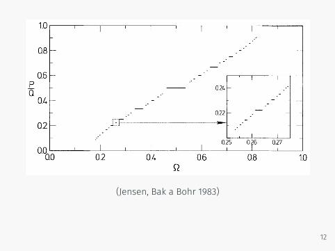
(Jensen, Bak a Bohr 1983)

12

simultaneously (Rossing, 1990). To examine how the brainstemresponse represents the envelope periodicity of the stimulus, weevaluated the temporal regularity of the FFR using the autocor-relational analysis. The running autocorrelograms for musician

and nonmusician groups are plotted inFigures 6A and 7A, with red indicating thehighest autocorrelations (periodicity). Forthe consonant interval, both groupsshowed the highest autocorrelation at 30.2ms, the dominant envelope periodicity ofthe stimulus. There was no significantgroup difference in the strength of theenvelope periodicity (t test, p ! 0.39; mu-sicians, 0.787; nonmusicians, 0.816).However, the morphology of the autocor-relation function was found to differ be-tween the two groups. This difference isevident in Figure 6A: the band of color"30.2 ms is sharper (i.e., narrower) for themusicians and broader for the nonmusi-cians, suggesting that the phase-locked ac-tivity to the temporal envelope is more ac-curate (i.e., sharper) in musicians thannonmusicians (cf. Krishnan et al., 2005).The sharpness of the autocorrelation func-tion showed a significant group difference(t test, p # 0.05; musicians, 0.395; nonmu-sicians, 0.521), i.e., the width was sharperin musicians (Fig. 6A). Moreover, therewas a significant correlation between yearsof musical training and the sharpness (r !$0.52, p # 0.05), such that the longer anindividual has been practicing music, thesharper the function (Fig. 6B). Of particu-lar interest is that nonmusicians showedstrong periodicities not only at intervals of30.2 ms but also every 10 ms. This 10 msperiod corresponds to 99 Hz (the lowertone, G). Thus, it is assumed that the peri-odicity at 30.2 ms for the nonmusicians isdriven in part by the robust neural phaselocking to the period of the lower tone, G.Thus, to isolate the periodicity at 30.2 ms,we calculated the change in periodicityfrom 30.2 ms (r1) to 10 ms (r2) using (r1 $r2)/(r1 % r2). Using this metric, we found asignificant group difference between mu-sicians and nonmusicians: musiciansshowed higher values than nonmusicians(ANOVA, F ! 6.7, p # 0.05). In addition,these values were positively correlatedwith years of musical training (r ! 0.454,p # 0.05).

In the autocorrelogram of the responseto the dissonant interval, the two highestperiodicities of both musicians and non-musicians matched the pattern in thestimulus autocorrelation: musicians with54.15 ms (r ! 0.678) and 42.4 ms (r !0.550) and nonmusicians with 54 ms (r !0.706) and 42.6 ms (r ! 0.611). Group dif-ferences were not significant. Autocorrelo-grams of the two groups are illustrated in

Figure 7A (left, musicians; right, nonmusicians). Here, musiciansalso exhibited sharper phase locking to the more dominant pe-riod of the stimulus, 54.1 ms (t test, p # 0.01; musicians, 0.453;nonmusicians, 0.647). In addition, the sharpness of the autocor-

Figure 2. Stimulus and response spectra for the consonant (A) and the dissonant (B) intervals. The response spectrum displaysthe average of all 26 subjects. The stimulus and response spectral amplitudes are scaled relative to their respective maximumamplitudes. Parentheses denote combination tones that do not exist in stimuli. f1 denotes the lower tone and f2 denotes the uppertone of each interval. See also Table 1.

Figure 3. Musicians show heightened responses to the harmonics of the upper tone and sum tones in the consonant interval.A, Grandaverage spectra for musicians (red) and nonmusicians (black) for the consonant interval. f1 and f2 denote G and E. B, Amplitudes offrequencies showing significant group differences. Error bars represent&1 SE. C, Pearson’s correlations (r and p) between amplitudes andyears of musical training. Significant correlations appear in bold. D, Individual amplitudes of the second harmonic of E (top) and f2 % 3f1

(!E f0%G H3) (bottom) as a function of years of musical training for all subjects (n!26) including the amateur group. Filled black circlesrepresent nonmusicians, open black circles amateur musicians, and red circles represent musicians.

Lee et al. • Selective Subcortical Enhancement in Musicians J. Neurosci., May 6, 2009 • 29(18):5832–5840 • 5835

(Lee et al. 2009)

13

1fdudt = f (u, v,λ)

+ εp(u, v,ρ, ε)

1fdvdt = g(u, v,λ)

+ εq(u, v,ρ, ε)

3.4 The normal form of the Hopf bifurcation 87

Finally, using the representation z = ρeiϕ, we obtain

z = ρeiϕ + ρiϕeiϕ,

orρeiϕ + iρϕeiϕ = ρeiϕ(α + i− ρ2),

which gives the polar form of system (3.6):!

ρ = ρ(α− ρ2),ϕ = 1.

(3.8)

Bifurcations of the phase portrait of the system as α passes through zerocan easily be analyzed using the polar form, since the equations for ρ andϕ in (3.8) are uncoupled. The first equation (which should obviously beconsidered only for ρ ≥ 0) has the equilibrium point ρ = 0 for all values ofα. The equilibrium is linearly stable if α < 0; it remains stable at α = 0but nonlinearly (so the rate of solution convergence to zero is no longer ex-ponential); for α > 0 the equilibrium becomes linearly unstable. Moreover,there is an additional stable equilibrium point ρ0(α) =

√α for α > 0. The

second equation describes a rotation with constant speed. Thus, by super-position of the motions defined by the two equations of (3.8), we obtain thefollowing bifurcation diagram for the original two-dimensional system (3.6)(see Figure 3.5). The system always has an equilibrium at the origin. Thisequilibrium is a stable focus for α < 0 and an unstable focus for α > 0.At the critical parameter value α = 0 the equilibrium is nonlinearly stableand topologically equivalent to the focus. Sometimes it is called a weaklyattracting focus. This equilibrium is surrounded for α > 0 by an isolatedclosed orbit (limit cycle) that is unique and stable. The cycle is a circle ofradius ρ0(α) =

√α. All orbits starting outside or inside the cycle except

at the origin tend to the cycle as t → +∞. This is an Andronov-Hopfbifurcation.

This bifurcation can also be presented in (x, y, α)-space (see Figure 3.6).The appearing α-family of limit cycles forms a paraboloid surface.

x1

x2 x2

x1

x2

x1

α = 0 α > 0α < 0

FIGURE 3.5. Supercritical Hopf bifurcation.(Kuznetsov 1998)

14

1fdudt = f (u, v,λ)

+ εp(u, v,ρ, ε)

1fdvdt = g(u, v,λ)

+ εq(u, v,ρ, ε)






ρ = ρ(α− ρ2),ϕ = 1.

(3.8)







x1

x2 x2

x1

x2

x1

α = 0 α > 0α < 0

FIGURE 3.5. Supercritical Hopf bifurcation.(Kuznetsov 1998) 14

1fdudt = f (u, v,λ) + εp(u, v,ρ, ε)

1fdvdt = g(u, v,λ) + εq(u, v,ρ, ε)






ρ = ρ(α− ρ2),ϕ = 1.

(3.8)







x1

x2 x2

x1

x2

x1

α = 0 α > 0α < 0

FIGURE 3.5. Supercritical Hopf bifurcation.(Kuznetsov 1998) 14

1fdudt = f (u, v,λ) + εp(u, v,ρ, ε)

1fdvdt = g(u, v,λ) + εq(u, v,ρ, ε)

(u, v) 7→ (z, z),λ 7→ (a,b,d),ρ 7→ (x, x), Taylorův rozvoj

15

1fdzdt

= z(a+ b|z|2 +∞∑k=0

dkεk+1|z|2k+4) +∑k>0

√ε|k|−1

(z x x

)k

8.3 Bautin (generalized Hopf) bifurcation 313

1

3

2

1

23

H+

H -

β

T

T

β

0

0

1

2

FIGURE 8.7. Bautin bifurcation

and no cycles. Crossing the Hopf bifurcation boundary H− from region1 to region 2 implies the appearance of a unique and stable limit cycle,which survives when we enter region 3. Crossing the Hopf boundary H+creates an extra unstable cycle inside the first one, while the equilibriumregains its stability. Two cycles of opposite stability exist inside region 3and disappear at the curve T through a fold bifurcation that leaves a singlestable equilibrium, thus completing the circle.

The case s = 1 in (8.25) can be treated similarly or can be reduced tothe one studied by the transformation (z, β, t) !→ (z,−β,−t).

8.3.3 Effect of higher-order termsLemma 8.5 The system

z = (β1 + i)z + β2z|z|2 ± z|z|4 + O(|z|6)

is locally topologically equivalent near the origin to the system

z = (β1 + i)z + β2z|z|2 ± z|z|4. ✷

The proof of the lemma can be obtained by deriving the Taylor expan-sion of the Poincare map for the first system and analyzing its fixed points.It turns out that the terms of order less than six are independent of O(|z|6)terms and thus coincide with those for the second system. This means thatthe two maps have the same number of fixed points for corresponding pa-rameter values and that these points undergo similar bifurcations as the

(Kuznetsov 1998)

dk 7→ d

16

1fdzdt

= z(a+ b|z|2 +∞∑k=0

dkεk+1|z|2k+4) +∑k>0

√ε|k|−1

(z x x

)k8.3 Bautin (generalized Hopf) bifurcation 313

1

3

2

1

23

H+

H -

β

T

T

β

0

0

1

2

FIGURE 8.7. Bautin bifurcation

and no cycles. Crossing the Hopf bifurcation boundary H− from region1 to region 2 implies the appearance of a unique and stable limit cycle,which survives when we enter region 3. Crossing the Hopf boundary H+creates an extra unstable cycle inside the first one, while the equilibriumregains its stability. Two cycles of opposite stability exist inside region 3and disappear at the curve T through a fold bifurcation that leaves a singlestable equilibrium, thus completing the circle.

The case s = 1 in (8.25) can be treated similarly or can be reduced tothe one studied by the transformation (z, β, t) !→ (z,−β,−t).

8.3.3 Effect of higher-order termsLemma 8.5 The system

z = (β1 + i)z + β2z|z|2 ± z|z|4 + O(|z|6)

is locally topologically equivalent near the origin to the system

z = (β1 + i)z + β2z|z|2 ± z|z|4. ✷

The proof of the lemma can be obtained by deriving the Taylor expan-sion of the Poincare map for the first system and analyzing its fixed points.It turns out that the terms of order less than six are independent of O(|z|6)terms and thus coincide with those for the second system. This means thatthe two maps have the same number of fixed points for corresponding pa-rameter values and that these points undergo similar bifurcations as the

(Kuznetsov 1998)

dk 7→ d

16

1fdzdt

= z(a+ b|z|2 + dε|z|4∞∑k=0

(ε|z|2)k) +∑k>0

√ε|k|−1

(z x x

)k

geometrická řada∞∑k=0

(ε|z|2)k = 11− ε|z|2

, |z| <√1ε

17

1fdzdt

= z(a+ b|z|2 + dε|z|4

1− ε|z|2

)+∑k>0

√ε|k|−1

(z x x

)kLarge, Almonte a Velasco 2010; Lerud et al. 2014

18

by multiple nonlinear transformations is not redundant; informa-tion is added at every processing stage, and each stage wouldcontribute to perceptual processing in important, and possiblyunique ways.

While odd-order nonlinearities in the FFR are typicallyattributed to the cochlea, the generation site of even-order non-linearities is far less clear (Bhagat and Champlin, 2004). In ourmodel of the FFR, the absence of contribution of the cochlea andthe strictly even-order nature of the response are true by defi-nition. However, it is easy to see how this could be the case in thehuman auditory system as well: Every prominent frequency in allresponses can be generated by even-order interaction between

stimulus components (see Fig. 4). The response at 2f1 ! f2, forinstance, is a typical example of a cubic distortion product;however in this case the frequency 2f1 actually occurs in thestimuli as the second harmonic of f1. Thus the component at2f1 ! f2 could be a simple difference tone. If one compares all thenonlinearities in the response to the frequencies in the stimuli,the potential quadratic nature of all response frequencies is clear.As the generation of even-order nonlinearities in scalp-recordedpotentials is much more likely neural, possibly as a result ofenvelope-following, than that of odd-order nonlinearities, thesimilarity of our model FFR to the actual FFR is perhaps furtherexplained.

Fig. 4. Model & data comparison. Comparisons of model predictions and auditory brainstem responses of nonmusicians to (A) the consonant interval (99 Hz, 166 Hz) and (B) thedissonant interval (93 Hz, 166 Hz), and of musicians to (C) the consonant interval and (D) the dissonant interval. The labels above each spectral component refer only to their specificfrequencies as functions of the primaries, and do not necessarily reflect the generating processes of those components (see Discussion).

K.D. Lerud et al. / Hearing Research 308 (2014) 41e4946

(Lerud et al. 2014)

19

by multiple nonlinear transformations is not redundant; informa-tion is added at every processing stage, and each stage wouldcontribute to perceptual processing in important, and possiblyunique ways.

While odd-order nonlinearities in the FFR are typicallyattributed to the cochlea, the generation site of even-order non-linearities is far less clear (Bhagat and Champlin, 2004). In ourmodel of the FFR, the absence of contribution of the cochlea andthe strictly even-order nature of the response are true by defi-nition. However, it is easy to see how this could be the case in thehuman auditory system as well: Every prominent frequency in allresponses can be generated by even-order interaction between

stimulus components (see Fig. 4). The response at 2f1 ! f2, forinstance, is a typical example of a cubic distortion product;however in this case the frequency 2f1 actually occurs in thestimuli as the second harmonic of f1. Thus the component at2f1 ! f2 could be a simple difference tone. If one compares all thenonlinearities in the response to the frequencies in the stimuli,the potential quadratic nature of all response frequencies is clear.As the generation of even-order nonlinearities in scalp-recordedpotentials is much more likely neural, possibly as a result ofenvelope-following, than that of odd-order nonlinearities, thesimilarity of our model FFR to the actual FFR is perhaps furtherexplained.

Fig. 4. Model & data comparison. Comparisons of model predictions and auditory brainstem responses of nonmusicians to (A) the consonant interval (99 Hz, 166 Hz) and (B) thedissonant interval (93 Hz, 166 Hz), and of musicians to (C) the consonant interval and (D) the dissonant interval. The labels above each spectral component refer only to their specificfrequencies as functions of the primaries, and do not necessarily reflect the generating processes of those components (see Discussion).

K.D. Lerud et al. / Hearing Research 308 (2014) 41e4946

(Lerud et al. 2014)

20

TONAL ORGANIZATION IN MUSIC 343

this experiment can be compared with thatof Krumhansl and Shepard (1979). Corre-lations between the 12 different profilesshowed a very similar pattern of probe tonejudgments for the major chord element andthe three cadences in major, IV-V-I, II-V-I, and VI-V-I. The average correlation be-tween these (.896, p < .01) indicates a con-sistent pattern of ratings for these elements.The profile for the major scale was somewhatless similar, having an average correlationof .796 with the other major profiles. Con-sequently, we will take as the major key pro-file the average ratings given the 12 probetones for the major chord and the three ca-dences in major. This profile is shown at thetop of Figure 2, where the average probetone judgments are plotted with respect toC major. Of course, the profile for any othermajor key would be identical, except shiftedthe appropriate number of semitones up ordown. Similarly, the profiles for the minorchord and the cadences in minor were verymuch alike, with an average correlation of.910 (p < .01). Again, the minor scale profilewas less similar, with an average correlationof .727 with the others. Thus, the minor keyprofile, also shown in Figure 2, is the averageof the profiles for the minor chord and theminor cadences.

The major and minor key profiles sharea number of features with each other andalso with the scale-completion judgments ofKrumhansl and Shepard (1979). In both keyprofiles the tonic, C, received higher ratingsthan all the other tones: t(9) = 16.84 formajor, and t(9) = 13.42 for minor, p < .001for both. In addition, all nontonic scale tones(using the harmonic form for minor) hadhigher average ratings than did nondiatonictones: *(9) = 6.05 and 9.23, /?<.001, formajor and minor, respectively. Within theset of diatonic tones, the components of thetonic chord, C, E, and G in major and C,E* (D#), and G in minor, were judged asfitting more closely with the major and mi-nor elements than were the other diatonictones: *(9) = 16.28 and 9.77, p < .001, formajor and minor, respectively. Thus, the rat-ings in this study strongly confirmed the hi-erarchy obtained by Krumhansl and Shep-ard (1979). This hierarchy was also evidentin the multidimensional scaling solution oftones judged in a major scale context

MAJOR KEY PROFILE

I I I I I I I IC C" D D« E F F« G G1 A A( B

PROBE TONE

Figure 2. The obtained major and minor key profilesfrom the first experiment. (The profile for the major key[upper graph] is the average rating given each of the12 tones of the chromatic scale following a major chordand the three cadences [IV-V-I, II-V-I, and VI-V-I]in a major key. The minor key profile [lower graph] isaveraged over the minor chord and the three cadencesin minor. The profiles are shown with respect to C majorand minor, respectively.)

(Krumhansl, 1979) and is entirely consistentwith the qualitative predictions of musictheory.

Interkey distance. We next used the ma-jor and minor key profiles, which have beenshown to be extremely reliable and inter-pretable, as an indirect measure of interkeydistance. The correlations between the pro-files, shifted to the appropriate tonics, aretaken as a measure of this distance. To il-lustrate this process, Figure 3 shows the pro-file for C major superimposed on the profilefor A minor (the C minor profile shifteddown three half steps or equivalently up ninehalf steps). The ratings of the two profileswere then correlated. These two particularprofiles were quite similar, giving a high cor-relation, as would be expected for a majorkey and its relative minor. This same pro-cedure was applied to all major-major, ma-

(Krumhansl a Kessler 1982)

TONAL HIERARCHIES IN INDIAN MUSIC 403

This produced rating profiles for the 10 rags,which are plotted in Figure 5, averaged overall 16 subjects. The profiles for Indian andWestern listeners were quite similar; for in-dividual rags, the intergroup correlations av-eraged .871 and were significant (p < .01) foreach of the 10 rags. Consequently, the profilesshown in Figure 5 are those for the two groupscombined. Differences between the two groupsare described later.

Tonal hierarchies. A number of statisticaltests were performed to determine whether theratings from the experiment conformed to thepredicted tonal hierarchy. The series of testscan best be described with respect to Figure6, where each branch corresponds to a testperformed. The figure shows the average ratinggiven to the tones in each of the following sets:non-mat tones, that tones, Sa (C), Pa (G), vadi,

samvadi, and the remaining tHat tones. In theseanalyses, the ratings given to the tones in eachset were computed for each subject, averagedover the 10 rag contexts. The first test com-pared the ratings for that and non-that tones,finding a significant preference for that overnon-that tones, f(l, 15) = 129.16, p < .01.The non-that tones were then eliminated, andthe next analysis compared Sa (C) with theother that tones, showing a preference for Sa(C), the tonic, over the other that tones, F(\,15) = 39.30, p < .01. Sa (C) was then elim-inated and the next test showed a significantpreference for Pa (G) over the remaining thattones, F(l, 15) = 42.97, p < .01. After Pa (G)was eliminated, the next analysis showed asignificant preference for the vadi over the re-maining tones, F(l, 15) = 18.41, p < .01.However, once the vadi was eliminated, no

BHAIRAV

C C* D D* E F F* G C* A A* B

YAMAN

C C* D D* E F F* G C* A A* B

BILAVAL

C C* 0 D* E F F* G C* A A* B

KHAMAJ

C C* D D' E F F* C C* A A' B

KAFI

C C* D 0* E F F* G G* A A* 8

ASAVRI

C C#D D#E F F#G G* A A* B

BHAIRVI

C C* 0 0* E F F# G G* A A* B

TOD I

C C#0 0*E F F#G G#A A# B

PURVI

C C* D 0* E F F* G G* A A* B

MARVA

C C' D D* E F F* G G* A A* B

Figure 5. The obtained rating profiles for 10 rags. (Each profile consists of the ratings, averaged over 16subjects, given to the 12 chromatic scale tones in the context of each of the rags.)

(Castellano,Bharucha aKrumhansl 1984)

Tonal Schemata in the Perception of Music in Bali and in the West 155

Fig. 12. Results for the pelog 1, 2, and 3 contexts for the Western and Kokar groups. There is a close similarity between the responses for these two groups.

This content downloaded from 128.97.27.21 on Tue, 12 May 2015 23:04:34 UTCAll use subject to JSTOR Terms and Conditions

156 Edward J. Kessler, Christa Hansen, &c Roger N. Shepard

Fig. 13. Results for the slendro 1 and 2 contexts for the Western and Kokar groups. The Kokar group, but not the Western group, consistently rates the important gong tone higher than the other tones of the slendro scale.

This content downloaded from 128.97.27.21 on Tue, 12 May 2015 23:04:34 UTCAll use subject to JSTOR Terms and Conditions

(Kessler, Hansen aShepard 1984)

21

1fdzdt

= z(a+ b|z|2 + dε|z|4

1− ε|z|2

)+∑k>0

√ε|k|−1

(z x x

)k

z ≡ reıθ, 1fdzdt

= eıθ(1fdrdt + ır 1

fdθdt

), x ≡ ρeıθ

22

eıθ(1fdrdt + ır 1

fdθdt

)=

reıθ(α+ ıω + (β1 + ıδ1) r2 + (β2 + ıδ2)

εr4

1− εr2

)+

∑k>0

√ε|k|−1

(r ρ ρ

)keık·(−θ θ −θ

)

1fdθdt

23

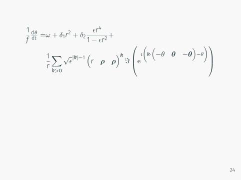
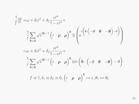
1fdθdt =ω + δ1r2 + δ2

εr4

1− εr2+

1r∑k>0

√ε|k|−1

(r ρ ρ

)k=

eı

(k·(−θ θ −θ

)−θ

)

=ω + δ1r2 + δ2εr4

1− εr2+

1r∑k>0

√ε|k|−1

(r ρ ρ

)ksin(k ·(−θ θ −θ

)− θ

)

f ≡ 1, δ1 ≡ δ2 ≡ 0,(r ρ ρ

)k7→ c, θ1 ↔ θ2

24


εr4

1− εr2+

1r∑k>0

√ε|k|−1

(r ρ ρ

)k=

eı

(k·(−θ θ −θ

)−θ

)=ω + δ1r2 + δ2

εr4

1− εr2+

1r∑k>0

√ε|k|−1

(r ρ ρ


)− θ

)

f ≡ 1, δ1 ≡ δ2 ≡ 0,(r ρ ρ

)k7→ c, θ1 ↔ θ2

24

dθ1dt = ω1 +

∑k>0

√ε|k|−1c sin

(k ·(−θ1 θ2 −θ2

)− θ1

)dθ2dt = ω2 +

∑k>0

√ε|k|−1c sin

(k ·(−θ2 θ1 −θ1

)− θ2

)

k 7→((m− 1) k 0

),((k− 1) m 0

)

25

dθ1dt = ω1 +

√εk+m−2c sin (kθ2 −mθ1)

dθ2dt = ω2 +

√εm+k−2c sin (mθ1 − kθ2)

202 E.W. Large

1 1.2 1.4 1.6 1.8 2

9:58:57:56:5 7:45:4 5:34:3 3:2 2:11:1

ω i / ω 0

16:15 17:12 16:9 15:89:8 8:56:5 5:4 5:34:3 3:2 2:11:1

cc

A)

B)

C CD E F G A B

pitch class (ET frequencies)

Fig. 4 Resonance regions. A) Bifurcation diagram showing natural resonances in a gradient frequency nonlinear oscillator array as a function of connection strength, c , and frequency ratio ω i /ω0. An infinite number of resonances are possible on this interval; the analysis considered the unison (1:1), the octave (2:1) and the twenty-five most stable resonances in between. B) Bifurcation diagram for a nonlinear oscillator network with internal connectivity reflecting an equal tempered chromatic scale. Internal connectivity can be learned via a Hebbian rule given passive exposure to melodies. Resonance regions whose center frequencies match ET ratios closely enough are predicted to be learned.

is coupling strength, a parameter that would be learned, and ε is the degree of nonlinearity in the coupling. This bifurcation analysis (Figure 4) assumes ε =1 (maximal nonlinearity) and plots resonance regions as a function of coupling strength on the vertical axis and relative frequency, ω i /ω0, on the horizontal axis. The phase equations (9) were used to derive the boundaries of the resonance regions, or Arnold tongues according to

km

± cm + kmk

.

The analysis varied oscillator frequency and coupling strength, assuming equal stimulation to each oscillator at a fixed frequency (the tonic, ω0). The result depicts the long-term stability of various resonances in the network, displayed as a bifurcation diagram called Arnold tongues (Figure 4A). It predicts how different pools of neural oscillators will respond by showing the boundaries of resonance

(Large 2010)

26

A Dynamical Systems Approach to Musical Tonality 207

C C# D D# E F F# G G# A A# B

2

4

6

C Majorst

abilit

y

r2=0.95ε =0.78


2

4

6

C Minor

stab

ility

r2=0.77ε =0.85

A) B)

Fig. 6 Comparison of theoretical stability predictions and human judgments of perceived stability for two Western modes. A) C major, B) C minor.

stability analysis, frequency ratios were fixed according to the previous analysis of learning (Figure 4B). It was further assumed that all the non-zero c were equal, effectively eliminating one free parameter (although in principle, the coupling strength, c , could be different for each resonance as a result of learning). Relative stability of each resonance was predicted by 2/)1( −+mkε , where k and m are the numerator and denominator of the frequency ratio, respectively, and 0 ≤ ε ≤ 1 is a parameter that controls nonlinear gain (Hoppensteadt & Izhikevich, 1997). The analysis assumed that each tone listeners heard as part of the context sequence was stabilized in the network, and those that were not heard were not stabilized. This assumption reflects the behavior of the network simulated in the previous analysis. Thus, each context tone received a stability value of

2/)1( −+mkε , and those that did not occur in the context sequence received a stability value of 0. For major and minor Western modes, the parameter ε was chosen to maximize the correlation ( r2 , different from oscillator amplitude, r, used previously) with the stability ratings of listeners. This provides a single parameter fit to the perceptual data on stability, shown in Figure 6.

Predicted stability matched the perceptual judgments well (C major: r2 = .95, p < .0001, ε = 0.78 ; C minor: r2 = .77, p < .001, ε = 0.85), as shown in Figure 6. In other words, the theoretical stability of higher-order resonances of nonlinear oscillators predicts empirically measured tonal stability for major and minor tonal contexts. This result is significant because it does not depend on the statistics of tone sequences, but instead it predicts the statistics of tone sequences, which are known to be highly correlated with stability judgments (Krumhansl, 1990).

5 Discussion

While the properties of nonlinear resonance predict the main perceptual features of tonality well, this theory makes two additional significant predictions: 1) that nonlinear resonance should be found in the human auditory system and 2) that animals with auditory systems similar to humans may be sensitive to tonal relationships. Recently, evidence has been found in support of both predictions.

Helmholtz (1863) described the cochlea as a time-frequency analysis mechanism that decomposes sounds into orthogonal frequency bands for further analysis by the central auditory nervous system. Von Bekesey (1960) observed

A Dynamical Systems Approach to Musical Tonality 207


2

4

6

C Major

stab

ility

r2=0.95ε =0.78


2

4

6

C Minor

stab

ility

r2=0.77ε =0.85

A) B)

Fig. 6 Comparison of theoretical stability predictions and human judgments of perceived stability for two Western modes. A) C major, B) C minor.

stability analysis, frequency ratios were fixed according to the previous analysis of learning (Figure 4B). It was further assumed that all the non-zero c were equal, effectively eliminating one free parameter (although in principle, the coupling strength, c , could be different for each resonance as a result of learning). Relative stability of each resonance was predicted by 2/)1( −+mkε , where k and m are the numerator and denominator of the frequency ratio, respectively, and 0 ≤ ε ≤ 1 is a parameter that controls nonlinear gain (Hoppensteadt & Izhikevich, 1997). The analysis assumed that each tone listeners heard as part of the context sequence was stabilized in the network, and those that were not heard were not stabilized. This assumption reflects the behavior of the network simulated in the previous analysis. Thus, each context tone received a stability value of

2/)1( −+mkε , and those that did not occur in the context sequence received a stability value of 0. For major and minor Western modes, the parameter ε was chosen to maximize the correlation ( r2 , different from oscillator amplitude, r, used previously) with the stability ratings of listeners. This provides a single parameter fit to the perceptual data on stability, shown in Figure 6.

Predicted stability matched the perceptual judgments well (C major: r2 = .95, p < .0001, ε = 0.78 ; C minor: r2 = .77, p < .001, ε = 0.85), as shown in Figure 6. In other words, the theoretical stability of higher-order resonances of nonlinear oscillators predicts empirically measured tonal stability for major and minor tonal contexts. This result is significant because it does not depend on the statistics of tone sequences, but instead it predicts the statistics of tone sequences, which are known to be highly correlated with stability judgments (Krumhansl, 1990).

5 Discussion

While the properties of nonlinear resonance predict the main perceptual features of tonality well, this theory makes two additional significant predictions: 1) that nonlinear resonance should be found in the human auditory system and 2) that animals with auditory systems similar to humans may be sensitive to tonal relationships. Recently, evidence has been found in support of both predictions.

Helmholtz (1863) described the cochlea as a time-frequency analysis mechanism that decomposes sounds into orthogonal frequency bands for further analysis by the central auditory nervous system. Von Bekesey (1960) observed

(Large 2010)

p < .01, but were lower than those for the Indian data,t(9)¼ 2.60, p¼ .01. We then computed the correlationsbetween the Western data and the durations of thetones in each raga. For the Western listeners, these cor-relations, mean r2(11) ¼ .80, min ¼ .72, max ¼ .88, allp < .01, were not significantly different from the corre-lations with the model (p ¼ .17). Finally, we comparedthe Indian and Western listeners’ correlations betweentheir ratings and tone durations. These were not signif-icantly different from one another (p ¼ .32). Thus, forthe Indian listeners the model outperformed the dura-tions, but not for the Western listeners, and both groupswere equal in the extent to which their data matched thedurations.

Next, the listener judgments were combined intoa single variable (10 ragas " 12 tones) for step-wiseregression analyses that included a wide range of factorsthat might be expected to generalize across cultures. The

factors considered were: predictions of the neurody-namic model (Equation 2), tone durations, harmonicity([k þ m – 1]/[km], see Gill & Purves, 2009), resonanceregion widths (Shapira Lots & Stone, 2008), and sixmeasures of consonance (Krumhansl, 1990, p. 57, Table3.1). For the neurodynamic model, the parameter ! wasfit to the average of the Indian and Western data foreach raga separately (see Method).

Because the stability ratings of Indian and Westernlisteners were highly correlated, the first regressionanalysis was performed to determine which variablescould account for the grand average ratings. Table 2(top) shows the results. The neurodynamic modelentered at step 1 and accounted for a highly significantamount of the variance for all ragas taken together,R2 (119) ¼ .79, p < .0001, as well as separately. Dura-tion came in at step 2 with both dynamics and durationcontributing significantly (at p < .0001) to fitting theaveraged data, R2 (118) ¼ .84, p < .0001, suggestinga combination of intrinsic dynamics and tone durationaccounts well for these patterns. Of the remaining vari-ables, the width of the resonance region (Shapira Lots& Stone, 2008) was the only one to contribute signif-icantly (at p ¼ .04) to the fit of the data. Because thecontribution is relatively modest and the resonanceregion model is closely related to the neurodynamicmodel conceptually, we did not consider it in the nextanalysis.

We then asked whether culturally specific variablesmight explain the remaining differences between theIndian and Western participants (bottom Table 2). Weconsidered several variables, including that (scale)membership, drone, the vadi and samvadi, which aretones emphasized in the individual raga, that might bemore salient for the Indian listeners, and the toneprofiles of several major and minor keys related to Cmajor and C minor that might be more salient for theWestern listeners. For the Indian data, two of thesemade highly significant contributions over and abovethe neurodynamic model and tone duration: whetherthe tone was in the drone (p ¼ .0002; the p-valuesgiven are those when the variable was first addedto the model) and whether the tone was in the that(p < .0001). The former shows an appreciation of thecentral role of the drone in anchoring melodies inthe style; the latter reflects the concept of scale mem-bership. For the Western data, two factors made sig-nificant contributions: the tone profiles of C minor(p ¼ .005) and G major (p ¼ .03), which reflect theWestern concept of major and minor scales. The fit ofthe full regression models to the respective data isshown in Figures 4 and 5.

FIGURE 3. The fit of the neurodynamic model predictions and theduration statistics to the average data. Shown in the figure are thetone profiles for 10 North Indian ragas averaged across Indian andWestern listeners (circles), the predictions of stability (Equation 2) foreach raga, based on an analysis of mode-locking dynamics (dots) alongwith the ! value for the maximum correlation, and the predictions basedon the relative durations of tones (triangles).

326 Edward W. Large, Ji Chul Kim, Nicole Kristine Flaig, Jamshed J. Bharucha, & Carol Lynne Krumhansl

(Large, Kim et al. 2016)

27


εr4

1− εr2+ . . .

1r∑k>0

√ε|k|−1

(r ρ ρ


)− θ

)

dθdt =fω

f ≡ f (1+ δ0),ff≡ f ,

τ ≡ f t,∆ ≡ δ0ω + (1+ δ0)

(δ1r2 + δ2

εr4

1− εr2

),

dθdτ = dθ

df t=1fdθdt ,

dθdτ = dθ

df t=1fdθdt

28


εr4

1− εr2+ . . .

1r∑k>0

√ε|k|−1

(r ρ ρ


)− θ

)dθdt =fω

f ≡ f (1+ δ0),ff≡ f ,

τ ≡ f t,∆ ≡ δ0ω + (1+ δ0)

(δ1r2 + δ2

εr4

1− εr2

),

dθdτ = dθ

df t=1fdθdt ,

dθdτ = dθ

df t=1fdθdt

28

dθdτ =ω +∆+ . . .

1+ δ0r

∑k>0

√ε|k|−1

(r ρ ρ


)− θ

)dθdτ =fω

(φ φ

)≡(θ θ

)−(ω fω

)τ

29

dφdτ =∆+

1+ δ0r

∑k>0

√ε|k|−1

(r ρ ρ

)k. . .

sin(k ·(− (ωτ + φ)

(fωτ + φ

)−(fωτ + φ

))− (ωτ + φ)

)

ϕ ≡ φ− h (ϕ,φ, τ)

9.3 Averaging the Phase Equations 263

is not periodic unless the vector of frequencies 0 is proportional to a vector of integers. The averaging theory is well developed for such quasi-periodic functions. It provides a time-dependent near-identity change of variables

¢ = cp + Eh(cp, t)

that transforms (9.22) to

where llT g( cp) = lim -T g(Ot + cp, 0) dt T->oo 0

is the "average" of g. Since 9 is a quasi-periodic function, this limit exists, and the function g is well defined. Its form depends crucially on the vector of frequencies o. It should be stressed that the full system (9.22) and the averaged system have distinct solutions (see Figure 9.7 for an illustration), which may diverge from each other even when they have identical initial

\

0 0 0 0 0 0 0 0 0 0 0 0 0 0 0 0 0 0 0 0 0 V VVVVVVVVVVVVVVVVVVVV(_tW

Figure 9.7. Numerical simulation of = E(cost - tP) and the averaged system cj; = -E!.p for E = 0.05).

states. Averaging theory guarantees their closeness on time scale 1/ E and even on the infinite time scale if additional requirements are imposed.

9.3.1 Averaging Theory

In this section we give a short exposition of the averaging theory that we use here. Even though we assume that ¢ E ']['n, the theory is valid if we substitute ']['n by any compact subset of jRn.

There is an intimate relationship between averaging and normal form theories (Arnold 1982, Sanders and Verhulst 1985). Both theories employ a change of variables that simplifies the right-hand side of a dynamical system. The normal form theory provides a change of variables that removes nonresonant monomials. Averaging theory provides a change of variables that removes time-dependent terms, which are in some sense nonresonant too.

(Hoppensteadt a Izhikevich 1997)

30

dϕdτ

≈ limT→∞

1T

∫ T

0

dφdτ

dτ

(Hoppensteadt a Izhikevich 1997, Theorem 9.6)

31

dϕdτ ≈∆+

1+ δ0r

∑√ε|k|−1

(r ρ ρ

)ksin(k ·(−ϕ ϕ −ϕ

)− ϕ

)

(−f f −f

)· k = f

S = {m+ s | m ∈ M, s ∈ S0}

32

dϕdτ ≈∆+

1+ δ0r

∑√ε|k|−1

(r ρ ρ


)− ϕ

)(−f f −f

)· k = f

S = {m+ s | m ∈ M, s ∈ S0}

32

(1 4

)·(ξ1 ξ2

)−(2 3

)·(η1 η2

)= 4

(a1 a2

)·(ξ1 ξ2

)−(b1 b2

)·(η1 η2

)= c

208 M. Clauscn and A. Fortenbacher

[ I I -4 ,1 -3 ] -2 ,1 - I I~ 12 13 I 4 I 4 3 2 1- 0 -1 -2 -3 -4

b2 b2 bl

b2 b2 bl b~

a l

a]

a l a2 al a2

bl

a2

a2

Figure 2: graph representation as adjacency matrix

represented by a graph, and all additions and subtractions can be performed by following labelled edges. This method speeds up the completion procedure. But surprisingly, the formulation of computations as a graph problem yields a new very fast algorithm which no longer is a completion procedure.

The graph represenialion G(a, b, c) of an inhomogeneous linear diophantine equation (1) is a labelled digraph with set of nodes

{ d E Z [ -ma~(b ,c ) < d < maxa}

and set of labelled edges

{d24 d + a ~ [ d < 0, i _ < m } O { d ~ d - b j [ d > O , j <_n} .

Recall that for a computation (Pl,.. . ,PIl~Ii-l,s), the defect of any proposal pi is a node of this graph. An edge d -% d+ ai corresponds to incrementing a proposal (~_, ~7) at

4i, an edge d ~ d - bj to incrementing ~?j. For example, the equation with a = (1, 4), b = (2, 3), c = 4 has a graph representation given in Figure 2.

Simi]iar to the description of minimal solutions as computations (Section 2) we now want to state a correspondence between solutions and walks in G(a ,~ c). Equivalent to the greatest computation for a given minimal solution s is a monotone walk in G(a, ~ c):

is monotone if the conditions

d k < 0 anddk, < O ~ ik < i~, d~ > 0 anddk, > 0 ~ j k <j~,

hold for all 1 _< k < k' _< l. t~oughly speaking, a monotone walk first follows edges with a lower labelling. In the graph given by Figure 2 both

O~2~4.~h2b_~_122~3b_~2 0

(Clausen a Fortenbacher 1989)

33

(1 4

)·(ξ1 ξ2

)−(2 3

)·(η1 η2

)= 4(

a1 a2)·(ξ1 ξ2

)−(b1 b2

)·(η1 η2

)= c


[ I I -4 ,1 -3 ] -2 ,1 - I I~ 12 13 I 4 I 4 3 2 1- 0 -1 -2 -3 -4

b2 b2 bl

b2 b2 bl b~

a l

a]

a l a2 al a2

bl

a2

a2




{ d E Z [ -ma~(b ,c ) < d < maxa}









O~2~4.~h2b_~_122~3b_~2 0


33

(1 4

)·(ξ1 ξ2

)−(2 3

)·(η1 η2

)= 4(

a1 a2)·(ξ1 ξ2

)−(b1 b2

)·(η1 η2

)= c


[ I I -4 ,1 -3 ] -2 ,1 - I I~ 12 13 I 4 I 4 3 2 1- 0 -1 -2 -3 -4

b2 b2 bl

b2 b2 bl b~

a l

a]

a l a2 al a2

bl

a2

a2




{ d E Z [ -ma~(b ,c ) < d < maxa}









O~2~4.~h2b_~_122~3b_~2 0

(Clausen a Fortenbacher 1989) 33

dϕdτ

≈ ∆+1+ δ0r

∑k∈M

√ε|k|−1

(r ρ ρ


)− ϕ

)

δ1 ≡ δ2 ≡ 0, r ≡ ρi ≡√γ

34

dϕdτ

= δ0ω+(1+ δ0)∑k∈M

√ε|k|−1√

γ|k|−1 sin(k ·(−ϕ ϕ −ϕ

)− ϕ

)

εγ 7→ ε

35

dϕdτ

= δ0ω + (1+ δ0)∑k∈M

√ε|k|−1 sin

(k ·(−ϕ ϕ −ϕ

)− ϕ

)

(Jensen, Bak a Bohr 1983)

36

dϕdτ

= δ0ω + (1+ δ0)∑k∈M

√ε|k|−1 sin

(k ·(−ϕ ϕ −ϕ

)− ϕ

)

(Jensen, Bak a Bohr 1983) 36

120 E.W. Large

��

��

f��f�

c

Fig. 2. Bifurcation diagram showing natural resonances in a tonotopic nonlinear oscil-lator array as a function of connection strength and frequency ratio (adapted from [4])

where cij is complex, representing the magnitude and phase of the connectionbetween any two nonlinear oscillators at a point in time [33], and δij and kij

are real parameters representing the speed of change of the connection. Thevariables, zi and zj are the complex valued state variables of the two oscillatorsconnected by cij . Previous analysis of the learning rule suggested that as alistener experiences Western musical sequences, connections within and betweennetworks would essentially be pruned, learning the frequencies of Western equaltemperament (ET). However, no experiments with learning were reported [4].

frequency

neuraloscillators

DCN

IC

memory

cochlea

efferentafferent

internal

stimulus

Fig. 3. Model architecture of phase-locking neural dynamics in the auditory system.Fixed connections are shown in gray, learned connections in black. Higher levels operateonly at lower frequencies, modeling deterioration of phase-locking at higher auditorylevels.

(Large 2011)

37

(A,A)-otevřený diskrétní dynamický systém (Spivak 2016):

• A ≡ {(f ,ϕ) | f ∈ Rn>0,ϕ ∈ Tn},

• S ≡ {(f , ϕ) | f : R>0 → R>0, ϕ : R>0 → T},• f upd : A2 × S→ S,• f rdt : S→ A

38


• A ≡ {(f ,ϕ) | f ∈ Rn>0,ϕ ∈ Tn},• S ≡ {(f , ϕ) | f : R>0 → R>0, ϕ : R>0 → T},

• f upd : A2 × S→ S,• f rdt : S→ A

38


• A ≡ {(f ,ϕ) | f ∈ Rn>0,ϕ ∈ Tn},• S ≡ {(f , ϕ) | f : R>0 → R>0, ϕ : R>0 → T},• f upd : A2 × S→ S,

• f rdt : S→ A

38


• A ≡ {(f ,ϕ) | f ∈ Rn>0,ϕ ∈ Tn},• S ≡ {(f , ϕ) | f : R>0 → R>0, ϕ : R>0 → T},• f upd : A2 × S→ S,• f rdt : S→ A

38

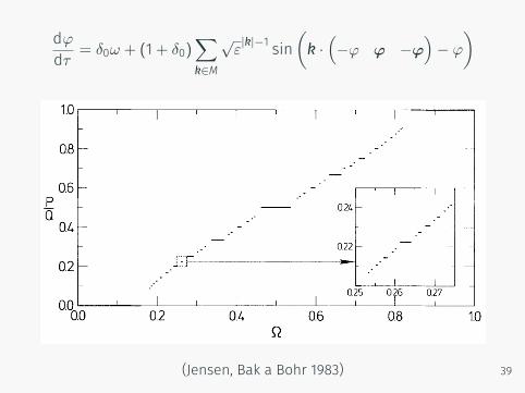
dϕdτ

= δ0ω + (1+ δ0)∑k∈M

√ε|k|−1 sin

(k ·(−ϕ ϕ −ϕ

)− ϕ

)


J = (1+ δ0)∑k∈M

√ε|k|−1

(−k1 − 1) cos(k ·(−ϕ ϕ −ϕ

)− ϕ

)


[ I I -4 ,1 -3 ] -2 ,1 - I I~ 12 13 I 4 I 4 3 2 1- 0 -1 -2 -3 -4

b2 b2 bl

b2 b2 bl b~

a l

a]

a l a2 al a2

bl

a2

a2




{ d E Z [ -ma~(b ,c ) < d < maxa}









O~2~4.~h2b_~_122~3b_~2 0


40

J = (1+ δ0)∑k∈M

√ε|k|−1

(−k1 − 1) cos(k ·(−ϕ ϕ −ϕ

)− ϕ

)208 M. Clauscn and A. Fortenbacher

[ I I -4 ,1 -3 ] -2 ,1 - I I~ 12 13 I 4 I 4 3 2 1- 0 -1 -2 -3 -4

b2 b2 bl

b2 b2 bl b~

a l

a]

a l a2 al a2

bl

a2

a2




{ d E Z [ -ma~(b ,c ) < d < maxa}









O~2~4.~h2b_~_122~3b_~2 0


40

dϕdτ

= δ0ω + (1+ δ0)∑k∈M

√ε|k|−1 sin

(k ·(−ϕ ϕ −ϕ

)− ϕ

)


matice ekvilibrií Mij ≡ #{s ∈ S | f rdt(s) = j, f upd(i, s) = s}(Spivak 2016)

42

120 E.W. Large

��

��

f��f�

c

Fig. 2. Bifurcation diagram showing natural resonances in a tonotopic nonlinear oscil-lator array as a function of connection strength and frequency ratio (adapted from [4])

where cij is complex, representing the magnitude and phase of the connectionbetween any two nonlinear oscillators at a point in time [33], and δij and kij

are real parameters representing the speed of change of the connection. Thevariables, zi and zj are the complex valued state variables of the two oscillatorsconnected by cij . Previous analysis of the learning rule suggested that as alistener experiences Western musical sequences, connections within and betweennetworks would essentially be pruned, learning the frequencies of Western equaltemperament (ET). However, no experiments with learning were reported [4].

frequency

neuraloscillators

DCN

IC

memory

cochlea

efferentafferent

internal

stimulus

Fig. 3. Model architecture of phase-locking neural dynamics in the auditory system.Fixed connections are shown in gray, learned connections in black. Higher levels operateonly at lower frequencies, modeling deterioration of phase-locking at higher auditorylevels.

ϕin : ((astim,aeff),aaff) 7→ (astim,aeff,aaff)

ϕout : aaff → aaff

Nij =∑

k∈ϕout−1(j)

M ϕin(i,k) k = M ϕin(i,j) j

(Spivak 2016)

43

Mary A. Castellano, Jamshed J. Bharucha aCarol L. Krumhansl. “Tonal hierarchies in the music ofnorth India”. In: Journal of Experimental Psychology.General 113.3 (1984), s. 394.

M. Clausen a A. Fortenbacher. “Efficient solution of lineardiophantine equations”. In: Journal of SymbolicComputation 8.1–2 (čvc—srp. 1989), s. 201–216. doi:10.1016/S0747-7171(89)80025-2.

Robert E. Ecke, J. Doyne Farmer a David K. Umberger.“Scaling of the Arnold tongues”. In: Nonlinearity 2.2(1989), s. 175.

44

http://dx.doi.org/10.1016/S0747-7171(89)80025-2

Frank C. Hoppensteadt a Eugene M. Izhikevich. Weaklyconnected neural networks. Sv. 126. AppliedMathematical Sciences. Springer-Verlag New York, 1997.doi: 10.1007/978-1-4612-1828-9.

M. Høgh Jensen, Per Bak a Tomas Bohr. “Complete devil’sstaircase, fractal dimension, and universality ofmode-locking structure in the circle map”. In: PhysicalReview Letters 50.21 (1983), s. 1637.

Edward J. Kessler, Christa Hansen a Roger N. Shepard.“Tonal schemata in the perception of music in Bali andin the West”. In: Music Perception. An InterdisciplinaryJournal 2.2 (1984), s. 131–165.

45

http://dx.doi.org/10.1007/978-1-4612-1828-9

Carol L. Krumhansl. “The psychological representation ofmusical pitch in a tonal context”. In: CognitivePsychology 11.3 (1979), s. 346–374.

Carol L. Krumhansl, Jamshed J. Bharucha aEdward J. Kessler. “Perceived harmonic structure ofchords in three related musical keys”. In: Journal ofExperimental Psychology. Human Perception andPerformance 8.1 (1982), s. 24.

Carol L. Krumhansl a Edward J. Kessler. “Tracing thedynamic changes in perceived tonal organization in aspatial representation of musical keys”. In: PsychologicalReview 89.4 (1982), s. 334.

Yuri A. Kuznetsov. Elements of applied bifurcation theory.Springer, 1998.

46

Edward W. Large. “A dynamical systems approach tomusical tonality”. In: Nonlinear Dynamics in HumanBehavior. Ed. Raoul Huys a Viktor K. Jirsa. Springer, 2010,s. 193–211.

Edward W. Large. “Musical tonality, neural resonance andHebbian learning”. In: International Conference onMathematics and Computation in Music. Springer. 2011,s. 115–125.

Edward W. Large, Felix V. Almonte a Marc J. Velasco. “Acanonical model for gradient frequency neural networks”.In: Physica D - Nonlinear Phenomena 239.12 (červ. 2010),s. 905–911. doi: 10.1016/j.physd.2009.11.015.

47

http://dx.doi.org/10.1016/j.physd.2009.11.015

Edward W. Large, Ji Chul Kim et al. “A neurodynamicaccount of musical tonality”. In: Music Perception. AnInterdisciplinary Journal 33.3 (2016), s. 319–331.

Kyung Myun Lee et al. “Selective subcorticalenhancement of musical intervals in musicians”. In:Journal of Neuroscience 29.18 (2009), s. 5832–5840.

Fred Lerdahl a Carol L. Krumhansl. “Modeling tonaltension”. In: Music Perception. An InterdisciplinaryJournal 24.4 (2007), s. 329–366.

Karl D. Lerud et al. “Mode-locking neurodynamics predicthuman auditory brainstem responses to musicalintervals”. In: Hearing Research 308.SI (ún. 2014),s. 41–49. doi: 10.1016/j.heares.2013.09.010.

48

http://dx.doi.org/10.1016/j.heares.2013.09.010

David I. Spivak. “The steady states of coupled dynamicalsystems compose according to matrix arithmetic”. Ver. 2.In: arXiv preprint arXiv:1512.00802 (24. ún. 2016). arXiv:1512.00802v2 [math.DS]. url:https://arxiv.org/abs/1512.00802v2 (cit.05. 04. 2017).

49

http://arxiv.org/abs/1512.00802v2

https://arxiv.org/abs/1512.00802v2

od hudby pÅ es mozek k diofantskÃ½m rovnicÃm - modelovÃ¡nÃ...

Documents