ocean data view user’s guide - santa barbara coastal...
TRANSCRIPT
Ocean Data View
User’s Guide
Version 3.0
May 17, 2005

Version 3.0
License Agreement By downloading or using this Software, you agree to be bound by the following legal agreement between you and the Alfred-Wegener-Institute for Polar and Marine Research (AWI). If you do not agree to the terms of this Agreement, do not download or use the Software. 1. SCIENTIFIC USE AND TEACHING Ocean Data View can be used free of charge for non-commercial, non-military research and teaching purposes. If you use the software for your scientific work, you must reference Ocean Data View in your publications as follows: Schlitzer, R., Ocean Data View, http://www.awi-bremerhaven.de/GEO/ODV, 2005. 2. COMMERCIAL AND MILITARY USE For the use of Ocean Data View or any of its components for commercial or military applications and products, a special, written software license is needed. Please contact the address below for further information. 3. REDISTRIBUTION Redistribution of the Ocean Data View software on CD-ROM, DVD, or other electronic media or the Internet is not per-mitted without the prior written consent of the AWI. Please contact the address below for further information. 4. WARRANTY DISCLAIMER THE ODV SOFTWARE IS PROVIDED "AS IS" WITHOUT WARRANTY OF ANY KIND, EITHER EXPRESSED OR IMPLIED, INCLUDING, BUT NOT LIMITED TO, THE IMPLIED WARRANTIES OF MERCHANTABILITY AND FITNESS FOR A PARTICULAR PURPOSE. THE ENTIRE RISK AS TO THE QUALITY AND PERFORMANCE OF THE SOFTWARE IS WITH YOU. SHOULD THE SOFTWARE PROVE DEFECTIVE, YOU ASSUME THE COST OF ALL NECESSARY SERVICING, REPAIR OR CORRECTION. IN NO EVENT WILL AWI, ITS CONTRIBUTORS OR ANY ODV COPYRIGHT HOLDER BE LIABLE TO YOU FOR DAMAGES, INCLUDING ANY DIRECT, INDIRECT, GENERAL, SPECIAL, EXEMPLARY, INCIDENTAL OR CONSEQUENTIAL DAMAGES HOWEVER CAUSED AND ON ANY THEORY OF LIABILITY ARISING OUT OF THE USE OR INABILITY TO USE THE SOFTWARE (INCLUDING BUT NOT LIMITED TO LOSS OF DATA OR DATA BEING RENDERED INACCURATE OR LOSSES SUSTAINED BY YOU OR THIRD PARTIES, A FAILURE OF THE SOFTWARE TO OPERATE WITH ANY OTHER SOFTWARE OR BUSINESS INTERRUPTION). © 2005 Reiner Schlitzer, Alfred Wegener Institute, Columbusstrasse, 27568 Bremerhaven, Germany.
Email: [email protected]
ii

Ocean Data View User’s Guide
Contents INTRODUCTION .............................................................................................................................................. 1
1.1 GENERAL OVERVIEW ............................................................................................................................1 1.2 EASE OF USE .........................................................................................................................................1 1.3 DENSE DATA FORMAT...........................................................................................................................1 1.4 EXTENSIBILITY......................................................................................................................................1 1.5 DERIVED VARIABLES ............................................................................................................................1 1.6 PLOT TYPES...........................................................................................................................................2 1.7 ODV MODES.........................................................................................................................................2 1.8 GRAPHICS OUTPUT................................................................................................................................5 1.9 POINT ESTIMATION AND BOX AVERAGING............................................................................................5 1.10 NETCDF SUPPORT ................................................................................................................................5
2 INSTALLING AND RUNNING ODV.................................................................................................. 7
2.1 INSTALLING OCEAN DATA VIEW...........................................................................................................7 2.2 INSTALLING OPTIONAL PACKAGES........................................................................................................7 2.3 RUNNING OCEAN DATA VIEW...............................................................................................................7
3 ODV SCREEN LAYOUT ...................................................................................................................... 9
3.1 MAIN MENU ..........................................................................................................................................9 3.2 3-LINE TEXT WINDOW ........................................................................................................................10 3.3 GRAPHICS CANVAS .............................................................................................................................11 3.4 MODE TAB BAR ..................................................................................................................................13 3.5 STATUS BAR........................................................................................................................................13 3.6 CURRENT STATION AND CURRENT SAMPLE ........................................................................................13 3.7 PLOTTING ............................................................................................................................................14
4 ODV COLLECTIONS ......................................................................................................................... 15
4.1 ODV DATA CONCEPT .........................................................................................................................15 4.2 CREATING COLLECTIONS ....................................................................................................................16 4.3 COLLECTION FILES SUMMARY ............................................................................................................17 4.4 MIGRATING BETWEEN WINDOWS, UNIX AND MAC OS X..................................................................18
5 IMPORTING DATA............................................................................................................................ 19
5.1 ODV SPREADSHEET FILES ..................................................................................................................19 5.2 WOCE HYDROGRAPHIC DATA............................................................................................................19 5.3 WOD HYDROGRAPHIC DATA..............................................................................................................20 5.4 WOA94 HYDROGRAPHIC DATA..........................................................................................................20 5.5 SD2 HYDROGRAPHIC DATA ................................................................................................................21 5.6 OTHER HYDROGRAPHIC DATA ............................................................................................................21 5.7 IMPORT OPTIONS DIALOG ...................................................................................................................22
6 EXPORTING DATA............................................................................................................................ 24
6.1 SPREADSHEET FILES............................................................................................................................24 6.2 ODV COLLECTION ..............................................................................................................................24 6.3 ASCII LISTINGS ..................................................................................................................................24 6.4 EXPORTING X/Y/Z PLOT DATA ...........................................................................................................24 6.5 EXPORTING REFERENCE DATASETS ....................................................................................................24
7 DERIVED VARIABLES...................................................................................................................... 25
7.1 BUILT-IN DERIVED VARIABLES ...........................................................................................................25 7.2 DERIVED VARIABLE MACROS .............................................................................................................27 7.3 EXPRESSIONS.......................................................................................................................................29
8 INTERACTIVE CONTROLS AND ODV MODES.......................................................................... 31
8.1 CHOOSING CURRENT SAMPLE AND CURRENT STATION.......................................................................31
iii

Version 3.0
8.2 CHANGING VARIABLE SETTINGS.........................................................................................................31 8.3 CHANGING SELECTION CRITERIA........................................................................................................31 8.4 CHANGING MAP PROJECTIONS............................................................................................................32 8.5 FULL SCREEN STATION MAPS.............................................................................................................33 8.6 PROPERTY-PROPERTY PLOTS ..............................................................................................................34 8.7 ZOOMING AND AUTOMATIC SCALING .................................................................................................34 8.8 CHANGING WINDOW LAYOUT ............................................................................................................35 8.9 CHANGING DISPLAY OPTIONS.............................................................................................................35 8.10 PRINTING ............................................................................................................................................39 8.11 POSTSCRIPT FILES...............................................................................................................................39 8.12 GIF, PNG AND JPG FILES...................................................................................................................39 8.13 PRODUCING SCATTER PLOTS ..............................................................................................................40 8.14 DEFINING A SECTION ..........................................................................................................................40 8.15 PLOTTING A SECTION ..........................................................................................................................41 8.16 COLOR-ZOOMING................................................................................................................................42 8.17 COLOR MAPPING FUNCTION ...............................................................................................................42 8.18 DISPLAYING GRIDDED FIELDS ............................................................................................................43 8.19 DIFFERENCE FIELDS............................................................................................................................44 8.20 DEFINING ISO-SURFACES ....................................................................................................................44 8.21 PLOTTING SURFACE DISTRIBUTIONS...................................................................................................45
9 NETCDF SUPPORT............................................................................................................................ 47
9.1 NETCDF OVERVIEW...........................................................................................................................47 9.2 USING NETCDF FILES .........................................................................................................................47
10 MANIPULATING COLLECTIONS.................................................................................................. 51
10.1 CHANGING THE SET OF COLLECTION VARIABLES ...............................................................................51 10.2 SORTING AND CONDENSING................................................................................................................51 10.3 DELETING SELECTED STATION-SUBSET..............................................................................................51
11 UTILITIES ........................................................................................................................................... 52
11.1 DATA INVENTORY TABLES .................................................................................................................52 11.2 GEOSTROPHIC FLOWS .........................................................................................................................52 11.3 3D ESTIMATION ..................................................................................................................................52 11.4 BOX AVERAGING ................................................................................................................................53 11.5 FINDING OUTLIERS .............................................................................................................................53 11.6 FINDING DUPLICATE STATIONS...........................................................................................................53
12 GRAPHICS OBJECTS........................................................................................................................ 54
12.1 ANNOTATIONS ....................................................................................................................................54 12.2 LINES AND POLYGONS ........................................................................................................................55 12.3 RECTANGLES AND ELLIPSES ...............................................................................................................55 12.4 SYMBOLS ............................................................................................................................................55 12.5 SYMBOL SETS AND LEGENDS..............................................................................................................55
13 MORE … .............................................................................................................................................. 57
13.1 GAZETTEER OF UNDERSEA FEATURES ................................................................................................57 13.2 DRAG-AND-DROP................................................................................................................................57 13.3 ODV COMMAND FILES (BATCH MODE)..............................................................................................58 13.4 USING PATCHES ..................................................................................................................................59 13.5 2D ESTIMATION ..................................................................................................................................60 13.6 EDITING DATA ....................................................................................................................................60 13.7 CHANGING THE COLOR PALETTE ........................................................................................................62 13.8 GENERAL SETTINGS ............................................................................................................................62 13.9 DATA STATISTICS ...............................................................................................................................62 13.10 TEMPORAL DATA DISTRIBUTION PLOTS .........................................................................................65 13.11 ANIMATIONS ...................................................................................................................................65
iv

Ocean Data View User’s Guide
14 TIPS AND TRICKS ............................................................................................................................. 67
14.1 DATA QUALITY CONTROL WITH ODV ................................................................................................67 14.2 VISUALIZING DATA FROM XYZ ASCII FILES .....................................................................................67 14.3 OVERLAYING A PROPERTY DISTRIBUTION WITH CONTOUR LINES OF ANOTHER PROPERTY ................68 14.4 PRE-COMPUTING AND STORING NEUTRAL DENSITY VALUES IN COLLECTIONS...................................69 14.5 USING ODV GRAPHICS IN PUBLICATIONS AND WEB PAGES ...............................................................69 14.6 MAKING CRUISE MAPS .......................................................................................................................70 14.7 PREPARING CUSTOM COASTLINE AND BATHYMETRY FILES................................................................70
15 APPENDIX ........................................................................................................................................... 73
15.1 ODV DIRECTORY STRUCTURE ............................................................................................................73 15.2 QUALITY FLAG MAPPING ....................................................................................................................73 15.3 GENERIC ODV SPREADSHEET FORMAT...............................................................................................75 15.4 GENERAL ODV SPREADSHEET FORMAT .............................................................................................76 15.5 O4X EXCHANGE FORMAT ....................................................................................................................77 15.6 O3X EXCHANGE FORMAT ....................................................................................................................78 15.7 CONTROL SEQUENCES AND FUNCTIONS IN ODV ANNOTATIONS.........................................................79 15.8 HARDWARE REQUIREMENTS AND LIMITATIONS..................................................................................79
v

Version 3.0
List of Figures Figure 1-1: Full-screen station map drawn in MAP mode ..................................................................................2 Figure 1-2: Property-property plots of selected stations .....................................................................................3 Figure 1-3: Scatter plots showing the data of all stations in the map..................................................................3 Figure 1-4: Property distributions along sections ...............................................................................................4 Figure 1-5: Property distributions on iso-surfaces ..............................................................................................4 Figure 1-6: Arrow plot of historical shipdrift data ..............................................................................................5 Figure 3-1: The ODV application window...........................................................................................................9 Figure 3-2: The 3-line text window ....................................................................................................................10 Figure 3-3: Activation areas and contents of ODV popup windows. .................................................................11 Figure 3-4: The canvas menu.............................................................................................................................12 Figure 3-5: The map menu.................................................................................................................................12 Figure 3-6: The data plot menu .........................................................................................................................13 Figure 3-7: The mode tab bar ............................................................................................................................13 Figure 3-8: The status bar .................................................................................................................................13 Figure 4-1: The variables selection dialog box .................................................................................................16 Figure 4-2: The variables definition dialog box ................................................................................................17 Figure 5-1: The import options dialog box ........................................................................................................22 Figure 7-1: The Edit Expression dialog box ......................................................................................................30 Figure 8-1: The selection criteria dialog box ....................................................................................................32 Figure 8-2: Map of the Southern Ocean with cruise track of R.V. Polarstern ANT VIII/2 ................................33 Figure 8-3: Property-property plots of five selected stations from the South Atlantic Ventilation Experiment
(SAVE)........................................................................................................................................................34 Figure 8-4: The display options dialog box of the map .....................................................................................36 Figure 8-5: The display options dialog box of data plot windows (STATION mode) ........................................37 Figure 8-6: The display options dialog box of data plot windows (non-STATION mode) .................................38 Figure 8-7: The display options properties dialog box ......................................................................................39 Figure 8-8: Scatter plots showing the data of all stations in the map. One of the stations is highlighted using
symbol sets. ................................................................................................................................................40 Figure 8-9: The GEOSECS western Atlantic section .........................................................................................41 Figure 8-10: The WOCE A16 section ................................................................................................................42 Figure 8-11: The color mapping dialog box ......................................................................................................43 Figure 8-12: Weighted averaging of data values (red symbols) at a grid node (+). See text for details. ..........44 Figure 8-13: The iso-surface variables dialog box ............................................................................................45 Figure 8-14: Temperature and salinity distributions on iso-surfaces................................................................46 Figure 9-1: The netCDF emulation dialog (step 1 of 4) ....................................................................................48 Figure 9-2: The netCDF emulation dialog (step 2 of 4) ....................................................................................49 Figure 9-3: The netCDF emulation dialog (step 3 of 4) ....................................................................................49 Figure 9-4: The netCDF emulation dialog (step 4 of 4) ....................................................................................50 Figure 10-1: The collection variables definition dialog box..............................................................................51
vi

Ocean Data View User’s Guide
Figure 12-1: Sample scatter plot using symbols sets and legends to highlight the data of a particular station 56 Figure 13-1: Using patches to identify the extent of water masses ....................................................................60 Figure 13-2: The station header dialog box .......................................................................................................61 Figure 13-3: The data edit dialog box................................................................................................................61 Figure 13-4: The statistics dialog box................................................................................................................63 Figure 13-5: A sample data histogram...............................................................................................................63 Figure 13-6: A sample data distribution plot .....................................................................................................64 Figure 13-7: Temporal data distribution for the Reid and Mantyla data collection ..........................................65 Figure 14-1: Identification of outliers for a zonal section in the North Atlantic................................................67 Figure 14-2: Oxygen contour lines on top of color shaded phosphate distribution ...........................................68 Figure 14-3: Schematic diagram of an ODV coastline/bathymetry segment. ....................................................71
List of Tables Table 2-1: ODV command line arguments ...........................................................................................................7 Table 3-1: ODV popup windows ........................................................................................................................11 Table 4-1: The ODV station metadata fields. .....................................................................................................15 Table 4-2: Summary of ODV collection files ......................................................................................................17 Table 4-3: Summary of ODV configuration files ................................................................................................17 Table 7-1: List of built-in derived variables .......................................................................................................25 Table 8-1: Regular expression syntax for cruise labels......................................................................................32 Table 15-1: Mapping of ARGO-to-ODV quality codes ......................................................................................74 Table 15-2: Mapping of IGOSS-to-ODV quality codes .....................................................................................74 Table 15-3: Mapping of WOCE-to-ODV quality codes.....................................................................................74 Table 15-4: Mapping of WOD01-to-ODV “entire station” quality codes........................................................75 Table 15-5: Mapping of WOD01-to-ODV “individual observed-level” quality codes ....................................75 Table 15-6: Formatting control sequences in ODV annotations........................................................................79 Table 15-7: Available auto-functions in ODV annotations. ...............................................................................79 Table 15-8: ODV limitations (data collections and graphical display) .............................................................80
vii

Ocean Data View User’s Guide
Introduction
1.1 General Overview Ocean Data View (ODV) is a computer program for the interactive exploration and graphical display of oceanographic and other geo-referenced profile, sequence or gridded data. The multi-platform version of ODV runs on computers with the Windows (9x/NT/2000/XP), Linux, UNIX, and Mac OS X operating systems. ODV data collection and configuration files are platform independent. They can be created on and exchanged between any of the supported systems. ODV lets you interactively browse through large sets of station data. You can produce high-quality station-maps, general property-property plots of one or more stations, scatter plots of selected stations, property sections along arbitrary cruise tracks and property distributions on general iso-surfaces. ODV supports display of original scalar and vector data by colored dots, numerical data values or arrows. In addition, two fast gridding algorithms provide estimates on automatically generated rectangular grids, and allow color shading and contouring of tracer fields along sections and on iso-surfaces. A large num-ber of derived quantities can be calculated on-the-fly. These variables may be displayed and analyzed in the same way as the basic variables stored on disk.
1.2 Ease of Use ODV is designed to be flexible and easy-to-use. Users need not know the details of the internal data storage format nor are they required to have programming experience. ODV always displays a map of available sta-tions on the screen and facilitates navigating through the data by letting the user select stations, sections and iso-surfaces with the mouse. The screen layout and various other configuration features can be modified eas-ily, and favorite settings can be stored in configuration files for later use. ODV can create and manage very large data collections on relatively inexpensive, widely available and mobile hardware. Existing data collec-tions can be extended easily when new data arrive. ODV greatly facilitates data quality control and can also be useful for teaching and training.
1.3 Dense Data Format The ODV data format is optimized for variable-length, irregularly-spaced profile, sequence or station data. It provides dense storage and allows instant access to any station, even in very large data collections. The data format is flexible and accepts data for up to 50 variables in any individual data collection. Type and number of variables may vary from one collection to another. ODV maintains quality flags for every individual data value. These quality flags may be used by ODV for data quality filtering and permit exclusion of, for instance, bad or questionable data from the analysis. Numerical values and quality flags can be edited and modified easily. All modifications are logged. Inadvertent changes can be reversed, if necessary.
1.4 Extensibility ODV allows easy import of new data into existing collections and also allows easy export of data from a col-lection. Oceanographic data in the following widely used formats can directly be read into the ODV system:
• WOCE WHP data (distributed over the Internet by the WHPO at SCRIPPS), • World Ocean Database (distributed on CD-ROM and over the Internet by NODC), • World Ocean Atlas 1994 (WOA94; distributed on CD-ROM by NODC), • NODC SD2 data • Java Ocean Atlas spreadsheet format, • ODV spreadsheet format.
1.5 Derived Variables In addition to the basic measured variables stored in the data files, ODV can calculate and display a large number of derived variables. Algorithms for these derived variables are either coded in the ODV software (potential temperature, potential density, dynamic height (all referenced to arbitrary levels), neutral density, Brunt-Väisälä Frequency, sound speed, oxygen saturation, etc.) or are defined in user provided macro files or expressions. The macro language is easy and general enough to allow a large number of applications. Use of expressions and macro files for new derived quantities broadens the scope of ODV considerably and allows easy experimentation with new quantities not yet established in the scientific community. ODV provides a built-in macro editor that facilitates creation and modification of ODV macros.
1
Version 3.0
Any basic or derived variable may be displayed in one or more plots. In addition, any variable can be used to define iso-surfaces (e.g., depth horizons, isopycnals, isothermals or isohalines; property minimum or maxi-mum layers like, for instance, the intermediate water salinity minimum layer can be defined as iso-surfaces by use of the zero-crossing of the vertical derivative (a derived quantity) of these variables).
1.6 Plot Types ODV displays data in two basic ways: (1) either by showing the original data at the data locations as colored dots of user-defined size, numeric values, or arrows; or (2) by projecting the original data on variable resolu-tion or equidistant rectangular grids and then displaying the gridded fields. Method 1 produces the most ele-mentary and honest views of the data, instantly revealing occasional bad data values and regions of poor sam-pling. In contrast, method 2 produces nicer plots and avoids the overlapping of the colored dots that occurs in method 1, especially for large dot-sizes. It has to be noted, however, that the gridded fields of method 2 repre-sent data-products and that small-scale or extreme features in the data may be lost due to the gridding proce-dure. For both display-modes, ODV allows the export of section or surface data to ASCII files or the clipboard for use with dedicated gridding, shading and contouring software. For quick overviews over large data sets ODV also lets you produce animated GIF files of the map or arbitrary data plot windows.
1.7 ODV Modes ODV can operate in five different modes MAP, STATION, SCATTER, SECTION, and SURFACE. You can easily switch between these modes at any time by pressing keys F8 through F12 or by selecting one of the pre-defined layout templates via Configuration>Use Template from the main menu or Use Template from the canvas popup menu. The current mode and the active configuration file are always indicated in the right-most pane of the ODV status bar. STATION mode is the default mode (initial mode for new data collections).
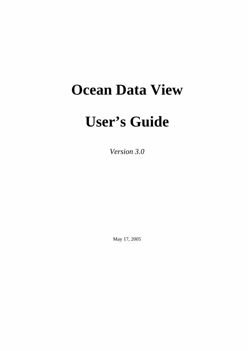
MAP mode is intended for full-page station maps and does not provide any data plots. Use this mode to pro-duce high quality cruise maps (define size and position of the map window, choose among five possible map projections, define appropriate coastline and topography settings, mark individual stations with station num-bers and cruise labels, produce printouts or PNG, JPG, and EPS PostScript files).
Figure 0-1: Full-screen station map drawn in MAP mode
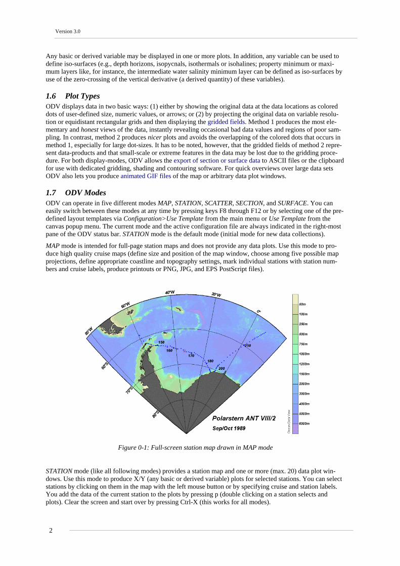
STATION mode (like all following modes) provides a station map and one or more (max. 20) data plot win-dows. Use this mode to produce X/Y (any basic or derived variable) plots for selected stations. You can select stations by clicking on them in the map with the left mouse button or by specifying cruise and station labels. You add the data of the current station to the plots by pressing p (double clicking on a station selects and plots). Clear the screen and start over by pressing Ctrl-X (this works for all modes).
2
Ocean Data View User’s Guide
Figure 0-2: Property-property plots of selected stations
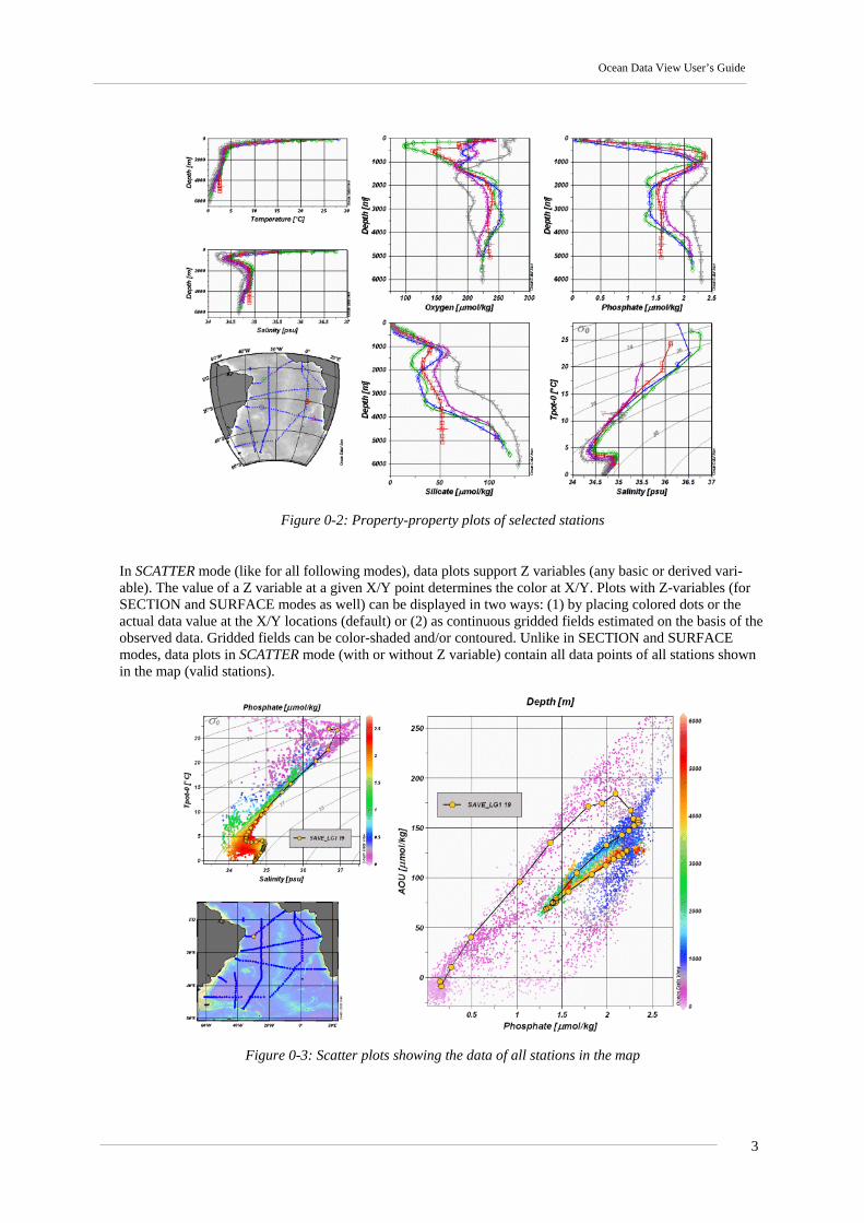
In SCATTER mode (like for all following modes), data plots support Z variables (any basic or derived vari-able). The value of a Z variable at a given X/Y point determines the color at X/Y. Plots with Z-variables (for SECTION and SURFACE modes as well) can be displayed in two ways: (1) by placing colored dots or the actual data value at the X/Y locations (default) or (2) as continuous gridded fields estimated on the basis of the observed data. Gridded fields can be color-shaded and/or contoured. Unlike in SECTION and SURFACE modes, data plots in SCATTER mode (with or without Z variable) contain all data points of all stations shown in the map (valid stations).
Figure 0-3: Scatter plots showing the data of all stations in the map
3

Version 3.0
SECTION mode also supports Z variables on data plots and allows all plot types of the SCATTER mode, but the set of stations used for the plots is restricted to a section band usually following a given cruise track. Sec-tion bands can be defined arbitrarily and their width can be adjusted to select the right set of stations. Use this mode to display property distributions along sections, property/property plots for all stations within a section and to calculate and investigate geostrophic velocities perpendicular to the cross-section.
Figure 0-4: Property distributions along sections
SURFACE mode lets you define surfaces in 3D (Longitude/Latitude/Depth) space defined as points of constant values of a given variable (e.g., depth, density, temperature, etc) and lets you display property distributions of other variables on this surface. In SURFACE mode you can also produce arbitrary property/property plots for the given surface.
Figure 0-5: Property distributions on iso-surfaces
4
Ocean Data View User’s Guide
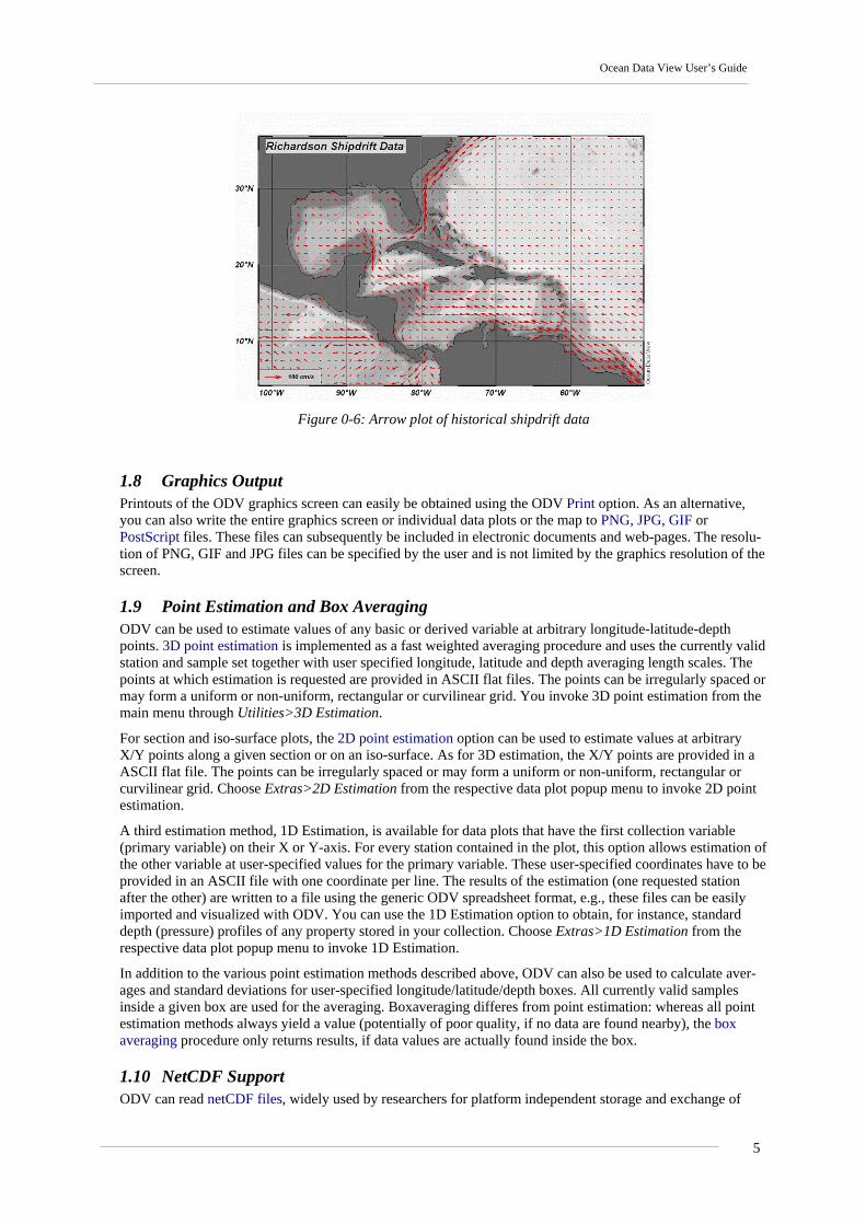
Figure 0-6: Arrow plot of historical shipdrift data
1.8 Graphics Output Printouts of the ODV graphics screen can easily be obtained using the ODV Print option. As an alternative, you can also write the entire graphics screen or individual data plots or the map to PNG, JPG, GIF or PostScript files. These files can subsequently be included in electronic documents and web-pages. The resolu-tion of PNG, GIF and JPG files can be specified by the user and is not limited by the graphics resolution of the screen.
1.9 Point Estimation and Box Averaging ODV can be used to estimate values of any basic or derived variable at arbitrary longitude-latitude-depth points. 3D point estimation is implemented as a fast weighted averaging procedure and uses the currently valid station and sample set together with user specified longitude, latitude and depth averaging length scales. The points at which estimation is requested are provided in ASCII flat files. The points can be irregularly spaced or may form a uniform or non-uniform, rectangular or curvilinear grid. You invoke 3D point estimation from the main menu through Utilities>3D Estimation.
For section and iso-surface plots, the 2D point estimation option can be used to estimate values at arbitrary X/Y points along a given section or on an iso-surface. As for 3D estimation, the X/Y points are provided in a ASCII flat file. The points can be irregularly spaced or may form a uniform or non-uniform, rectangular or curvilinear grid. Choose Extras>2D Estimation from the respective data plot popup menu to invoke 2D point estimation.
A third estimation method, 1D Estimation, is available for data plots that have the first collection variable (primary variable) on their X or Y-axis. For every station contained in the plot, this option allows estimation of the other variable at user-specified values for the primary variable. These user-specified coordinates have to be provided in an ASCII file with one coordinate per line. The results of the estimation (one requested station after the other) are written to a file using the generic ODV spreadsheet format, e.g., these files can be easily imported and visualized with ODV. You can use the 1D Estimation option to obtain, for instance, standard depth (pressure) profiles of any property stored in your collection. Choose Extras>1D Estimation from the respective data plot popup menu to invoke 1D Estimation.
In addition to the various point estimation methods described above, ODV can also be used to calculate aver-ages and standard deviations for user-specified longitude/latitude/depth boxes. All currently valid samples inside a given box are used for the averaging. Boxaveraging differes from point estimation: whereas all point estimation methods always yield a value (potentially of poor quality, if no data are found nearby), the box averaging procedure only returns results, if data values are actually found inside the box.
1.10 NetCDF Support ODV can read netCDF files, widely used by researchers for platform independent storage and exchange of
5

Version 3.0
geo-science data or model output. ODV lets you define one or more views of the data in the netCDF file by letting you select coordinates and variables from the file, subset the netCDF data by means of an easy-to-use netCDF emulation wizard. ODV then presents the contents of the netCDF file as if it was a native ODV collec-tion. The full suite of ODV’s analysis and visualization tools is available for the exploration of the netCDF data, and there is no need to translate and re-write the data first. Depending on the structure and contents of a netCDF file, different ODV emulations are possible. Settings of individual emulations can be saved on disk for later use. NetCDF files are platform independent and can be used on all ODV supported systems.
6
Ocean Data View User’s Guide
2 Installing and Running ODV
2.1 Installing Ocean Data View You run Ocean Data View either from an ODV run-time environment on a CD-ROM or DVD (the eWOCE directory on DVD 2 of the WOCE V3 data release contains such a run-time environment) or from an ODV installation on your computer. If you plan to use ODV regularly, you should install the software on your ma-chine. ODV installation files are available for Windows (9x/NT/2000/XP), Linux, UNIX, and Mac OS X sys-tems. Visit http://www.awi-bremerhaven.de/GEO/ODV/downloads-odvmp.html for the latest version. Installa-tion instructions are provided in INSTALL files.
2.2 Installing Optional Packages Complementary high-resolution coastline and topography files or ready-to-use data collections are available as optional packages (visit http://www.awi-bremerhaven.de/GEO/ODV/downloads-odvmp.html and http://www.awi-bremerhaven.de/GEO/ODV/downloads-data.html ). Again, see the INSTALL files for installa-tion instructions and further information.
2.3 Running Ocean Data View (1) Starting ODV Once ODV is installed on your system you can start the program in a number of ways.
On Windows, the installation procedure will create an ODV icon on your desktop and will automatically asso-ciate .var collection files with the ODV application. To launch ODV, you can double-click a .var file or the ODV desktop icon. Alternatively, you can also use the Start>Program Files>Ocean Data View (mp) option. You may drag the ODV desktop icon onto the Windows taskbar. Then, a single click on the taskbar ODV icon will start ODV.
Any ODV supported file can be dragged onto the ODV icon on the desktop or the Windows taskbar. This will start ODV and open the dragged file in a single operation. When ODV is running, you can drag an ODV sup-ported file onto the ODV window to open this file. Supported file types include ODV collections (.var), netCDF files (*.nc, *cdf), ODV spreadsheet files (.txt) and others.
On Linux, UNIX and Mac OS X systems you can create aliases or icons for the ODV executable odvmp or the ODV startup script file run_odv. Use methods specific to your operating system to create desktop, taskbar, or dock icons or aliases. The ODV executable odvmp is located in the bin_… directory of your ODV installa-tion (the “…” represents a system dependent suffix, e.g., macx on MacOS X or linux-i386 on Linux systems). Once a desktop or taskbar/dock icon is created you start ODV by double or single-clicking on the ODV icon. On most systems you can also drag-and-drop ODV collection .var files, netCDF files or any supported data import file onto the ODV icon.
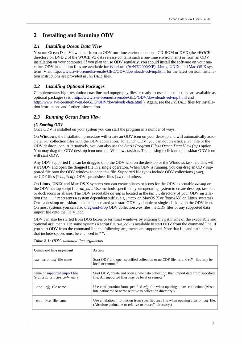
ODV can also be started from DOS boxes or terminal windows by entering the pathname of the executable and optional arguments. On some systems a script file run_odv is available to start ODV from the command line. If you start ODV from the command line the following arguments are supported. Note that file and path names that include spaces must be enclosed in “ “.
Table 2-1: ODV command line arguments
Command line argument Action
.var, .nc or .cdf file name Start ODV and open specified collection or netCDF file. nc and cdf files may be local or remote.
name of supported import file (e.g., .txt, .csv, .jos, .o4x, etc.)
Start ODV, create and open a new data collection, then import data from specified file. All supported files may be local or remote. 
-cfg .cfg file name Use configuration from specified .cfg file when opening a .var collection. (Abso-lute pathname or name relative to collection directory.)
-nce .nce file name Use emulation information from specified .nce file when opening a .nc or .cdf file. (Absolute pathname or relative to .nc/.cdf directory.)
7

Version 3.0
-x .cmd file name Start ODV and execute specified ODV command file.
-q Shutdown ODV after all command line arguments have been processed. ¶ Remote files are automatically downloaded to your local machine and then processed. You specify remote files using http://... or ftp://... type URLs. Note that if you are behind a firewall, a socket server software, such as SocksCap on Windows, must be used to launch ODV, if you want to access remote files.
(2) Quick Installation Dialog
When ODV runs for the first time, you will be prompted for the following Quick Installation information:
1. the full path-name of the directory that contains the bin_… directory (ODVMPHOME environment variable),
2. the full path-name of a directory on your disk which will be used by ODV during runtime to write temporary files (ODVMPTEMP environment variable). Note that you must have write permission for this directory. You can use the system tmp directory, or you can create a special directory on a local disk (e.g., /odvmptemp) for this purpose. The use of directories on network drives is not recom-mended because of network transmission delays.
3. the name of your computer,
4. your user or login name.
Press OK to finish the Quick Installation. Then customize ODV font and external programs settings using the Configuration>General Settings dialog. Press F1 or use option Help>User’s Guide, if you need help. Context sensitive help is provided, when you press the Help button on many ODV dialogs.
(3) Using ODV Once ODV is running, you open a particular data collection, netCDF file or any of the supported import data files using the File>Open option. A standard file-open dialog will appear, and you can choose the appropriate file type and file name to be opened. If you open a supported import data file, ODV will automatically create a new collection from the data in the specified file and will then open the newly created data collection. Note that after opening a collection, ODV loads the configuration settings from the most recent ODV session with this collection. Please note that this most recent configuration might apply station and sample selection filters. As a consequence, only a subset of the stations in the data collection may be shown in the station map. Use Configuration>Use Template>default to obtain a default map with all collection stations or use Configura-tion>Selection Criteria to modify the selection criteria and obtain a different station/sample subset.
You may load other, previously saved, configuration files using Configuration>Load Configuration, you may choose one of the pre-defined layout templates using Configuration>Use Template or you may change the various settings interactively using the Configuration menu options or the popup menus that appear when you right-click the mouse while over the canvas area, the map, or one of the data plots. On Mac OS X systems hold down the Alt key while clicking the mouse to simulate a right mouse button click.
In addition to opening local files with File>Open, you can also access remote datasets using the File>Open URL option. ODV will prompt you for a Uniform Resource Locator address (URL) pointing to a netCDF or supported import file and will then download and open the respective file. You may specify URLs with the http: or ftp: protocol identifiers. Note that if you are behind a firewall, you may need a socket server software, such as SocksCap on Windows, to complete http: or ftp: requests.
8
Ocean Data View User’s Guide
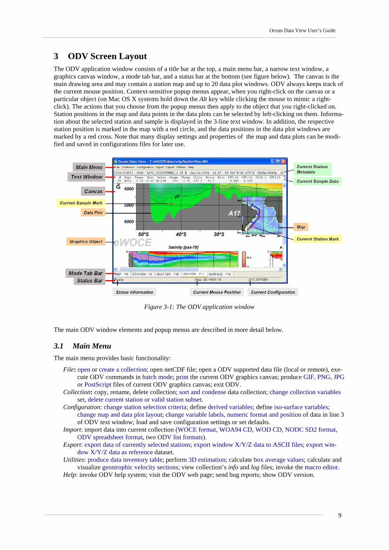
3 ODV Screen Layout The ODV application window consists of a title bar at the top, a main menu bar, a narrow text window, a graphics canvas window, a mode tab bar, and a status bar at the bottom (see figure below). The canvas is the main drawing area and may contain a station map and up to 20 data plot windows. ODV always keeps track of the current mouse position. Context-sensitive popup menus appear, when you right-click on the canvas or a particular object (on Mac OS X systems hold down the Alt key while clicking the mouse to mimic a right-click). The actions that you choose from the popup menus then apply to the object that you right-clicked on. Station positions in the map and data points in the data plots can be selected by left-clicking on them. Informa-tion about the selected station and sample is displayed in the 3-line text window. In addition, the respective station position is marked in the map with a red circle, and the data positions in the data plot windows are marked by a red cross. Note that many display settings and properties of the map and data plots can be modi-fied and saved in configurations files for later use.
Figure 3-1: The ODV application window
The main ODV window elements and popup menus are described in more detail below.
3.1 Main Menu The main menu provides basic functionality:
File: open or create a collection; open netCDF file; open a ODV supported data file (local or remote), exe-cute ODV commands in batch mode; print the current ODV graphics canvas; produce GIF, PNG, JPG or PostScript files of current ODV graphics canvas; exit ODV.
Collection: copy, rename, delete collection; sort and condense data collection; change collection variables set, delete current station or valid station subset.
Configuration: change station selection criteria; define derived variables; define iso-surface variables; change map and data plot layout; change variable labels, numeric format and position of data in line 3 of ODV text window; load and save configuration settings or set defaults.
Import: import data into current collection (WOCE format, WOA94 CD, WOD CD, NODC SD2 format, ODV spreadsheet format, two ODV list formats).
Export: export data of currently selected stations; export window X/Y/Z data to ASCII files; export win-dow X/Y/Z data as reference dataset.
Utilities: produce data inventory table; perform 3D estimation; calculate box average values; calculate and visualize geostrophic velocity sections; view collection’s info and log files; invoke the macro editor.
Help: invoke ODV help system; visit the ODV web page; send bug reports; show ODV version.
9
Version 3.0
3.2 3-Line Text Window
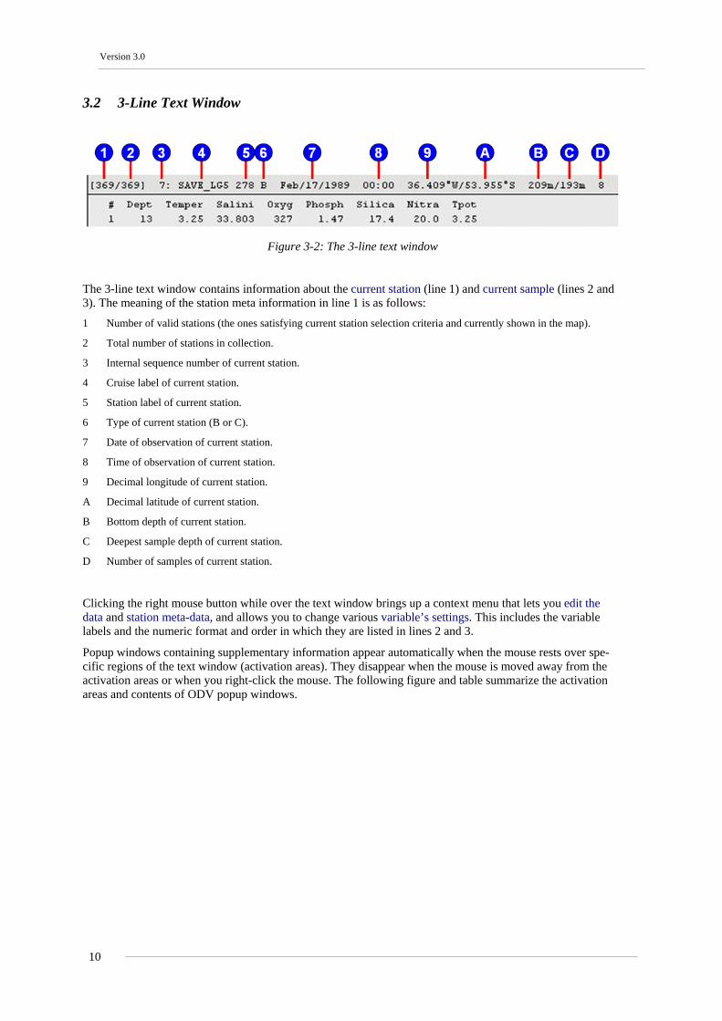
Figure 3-2: The 3-line text window
The 3-line text window contains information about the current station (line 1) and current sample (lines 2 and 3). The meaning of the station meta information in line 1 is as follows:
1 Number of valid stations (the ones satisfying current station selection criteria and currently shown in the map).
2 Total number of stations in collection.
3 Internal sequence number of current station.
4 Cruise label of current station.
5 Station label of current station.
6 Type of current station (B or C).
7 Date of observation of current station.
8 Time of observation of current station.
9 Decimal longitude of current station.
A Decimal latitude of current station.
B Bottom depth of current station.
C Deepest sample depth of current station.
D Number of samples of current station.
Clicking the right mouse button while over the text window brings up a context menu that lets you edit the data and station meta-data, and allows you to change various variable’s settings. This includes the variable labels and the numeric format and order in which they are listed in lines 2 and 3.
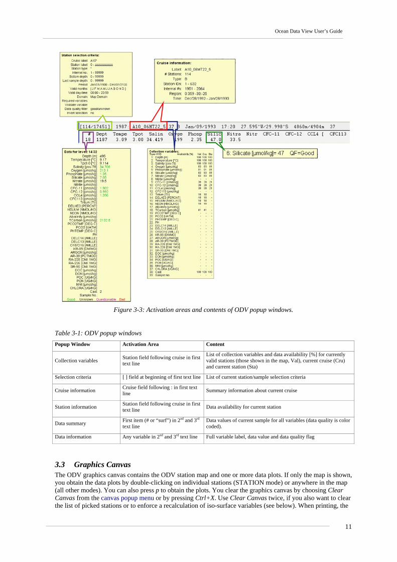
Popup windows containing supplementary information appear automatically when the mouse rests over spe-cific regions of the text window (activation areas). They disappear when the mouse is moved away from the activation areas or when you right-click the mouse. The following figure and table summarize the activation areas and contents of ODV popup windows.
10
Ocean Data View User’s Guide
Figure 3-3: Activation areas and contents of ODV popup windows.
Table 3-1: ODV popup windows Popup Window Activation Area Content
Collection variables Station field following cruise in first text line
List of collection variables and data availability [%] for currently valid stations (those shown in the map, Val), current cruise (Cru) and current station (Sta)
Selection criteria [ ] field at beginning of first text line List of current station/sample selection criteria
Cruise information Cruise field following : in first text line Summary information about current cruise
Station information Station field following cruise in first text line Data availability for current station
Data summary First item (# or “surf”) in 2nd and 3rd text line
Data values of current sample for all variables (data quality is color coded).
Data information Any variable in 2nd and 3rd text line Full variable label, data value and data quality flag
3.3 Graphics Canvas The ODV graphics canvas contains the ODV station map and one or more data plots. If only the map is shown, you obtain the data plots by double-clicking on individual stations (STATION mode) or anywhere in the map (all other modes). You can also press p to obtain the plots. You clear the graphics canvas by choosing Clear Canvas from the canvas popup menu or by pressing Ctrl+X. Use Clear Canvas twice, if you also want to clear the list of picked stations or to enforce a recalculation of iso-surface variables (see below). When printing, the
11

Version 3.0
ODV graphics canvas is mapped to the paper size of your printer.
You can arbitrarily resize the ODV application window by pressing the resize button in the upper right corner of the application window or by dragging the window frame. Horizontal and/or vertical scrollbars will appear on the graphics canvas if the ODV application window is smaller than the canvas area. Slide the scrollbars or drag the graphics canvas (press and hold down the left mouse button and move the mouse) to select the view-able canvas area.
Clicking the right mouse button (on a Mac OS X system hold down the Alt key and click the mouse) while over the map, the data plots or the canvas area invokes the following popup menus:
Figure 3-4: The canvas menu
On the canvas popup menu the following options are avail-able: • clear the graphics canvas and restore the station map.
when done twice, clears the list of picked stations (MAP and STATION modes), or enforces a re-calculation of iso-surface variables (SURFACE mode).
• produce GIF, PNG, JPG, or PostScript file for the entire graphics canvas,
• print the graphics canvas, • re-scale all windows to full-scale, • undo the last change, • define derived variables, • define iso-surface variables (SURFACE mode only), • change variable labels, numeric format and position of
data in line 3 of ODV text window, • add or manage the canvas graphics objects, • change map and data window layout, • save or load a configuration file, • exit ODV.
Figure 3-5: The map menu
On the map popup menu the following options are available: • zoom in and out map domain, • open map to full domain of collection, • produce standard, global map, • produce PostScript, GIF, PNG or JPG file of the map, • change station selection criteria, • change map display options (projection, topography and coast-
line settings, station annotation style), • define section (SECTION mode only), • select a new current station by name or internal number, • access the map’s Extras menu that lets you produce plots of
the stations temporal distribution, view map statistics, produce map animations, view Gazetteer data, add graphics objects to the map, and copy the map’s data to the clipboard.
12
Ocean Data View User’s Guide
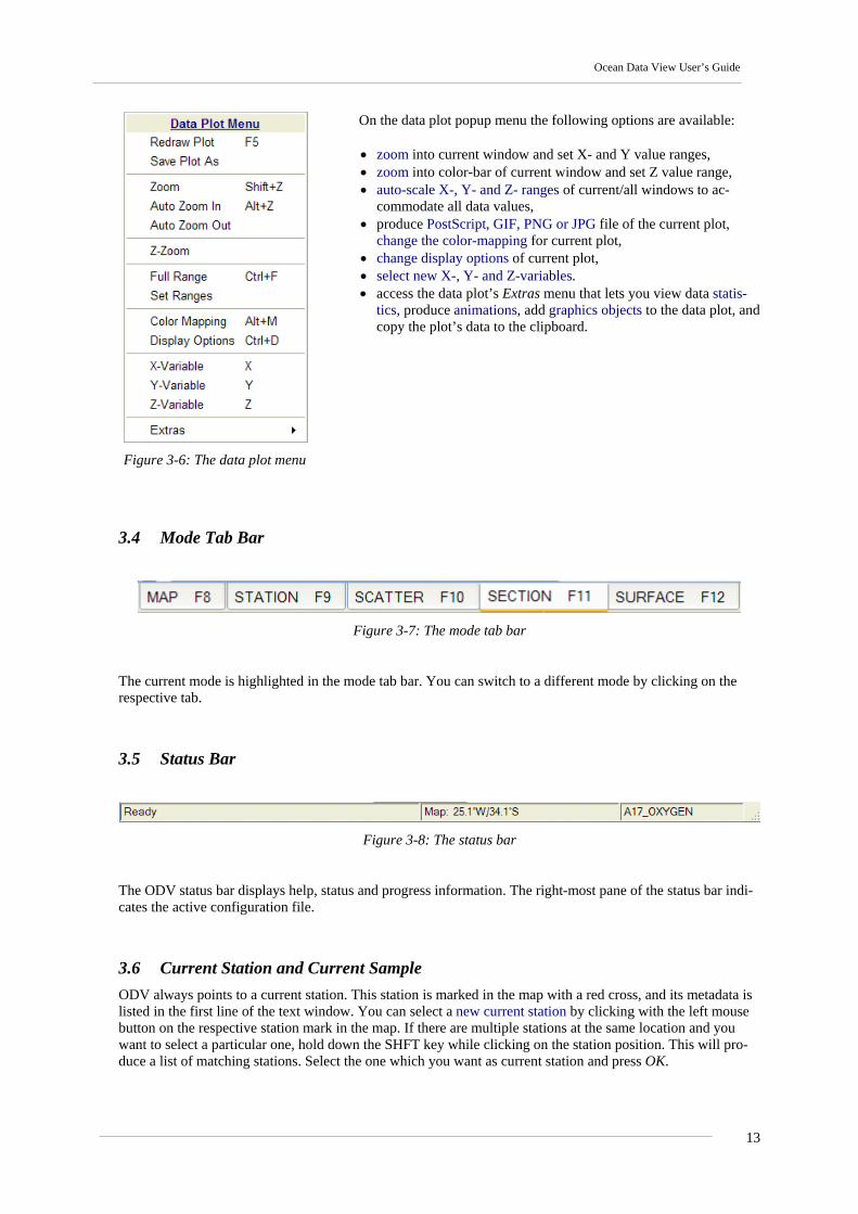
Figure 3-6: The data plot menu
On the data plot popup menu the following options are available: • zoom into current window and set X- and Y value ranges, • zoom into color-bar of current window and set Z value range, • auto-scale X-, Y- and Z- ranges of current/all windows to ac-
commodate all data values, • produce PostScript, GIF, PNG or JPG file of the current plot,
change the color-mapping for current plot, • change display options of current plot, • select new X-, Y- and Z-variables. • access the data plot’s Extras menu that lets you view data statis-
tics, produce animations, add graphics objects to the data plot, and copy the plot’s data to the clipboard.
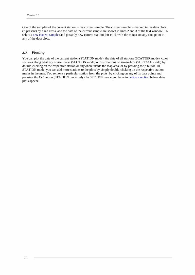
3.4 Mode Tab Bar
Figure 3-7: The mode tab bar
The current mode is highlighted in the mode tab bar. You can switch to a different mode by clicking on the respective tab.
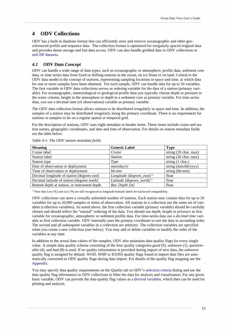
3.5 Status Bar
Figure 3-8: The status bar
The ODV status bar displays help, status and progress information. The right-most pane of the status bar indi-cates the active configuration file.
3.6 Current Station and Current Sample ODV always points to a current station. This station is marked in the map with a red cross, and its metadata is listed in the first line of the text window. You can select a new current station by clicking with the left mouse button on the respective station mark in the map. If there are multiple stations at the same location and you want to select a particular one, hold down the SHFT key while clicking on the station position. This will pro-duce a list of matching stations. Select the one which you want as current station and press OK.
13
Version 3.0
One of the samples of the current station is the current sample. The current sample is marked in the data plots (if present) by a red cross, and the data of the current sample are shown in lines 2 and 3 of the text window. To select a new current sample (and possibly new current station) left-click with the mouse on any data point in any of the data plots.
3.7 Plotting You can plot the data of the current station (STATION mode), the data of all stations (SCATTER mode), color sections along arbitrary cruise tracks (SECTION mode) or distributions on iso-surface (SURFACE mode) by double-clicking on the respective station or anywhere inside the map area, or by pressing the p button. In STATION mode, you can add more stations to the plots by simply double-clicking on the respective station marks in the map. You remove a particular station from the plots by clicking on any of its data points and pressing the Del button (STATION mode only). In SECTION mode you have to define a section before data plots appear.
14
Ocean Data View User’s Guide
4 ODV Collections ODV has a built-in database format that can efficiently store and retrieve oceanographic and other geo-referenced profile and sequence data. The collection format is optimized for irregularly spaced original data and provides dense storage and fast data access. ODV can also handle gridded data in ODV collections or netCDF datasets.
4.1 ODV Data Concept ODV can handle a wide range of data types, such as oceanographic or atmospheric profile data, sediment core data, or time series data from fixed or drifting stations in the ocean, on ice floats or on land. Central to the ODV data model is the concept of stations, representing sampling locations in space and time, at which data for one or more samples have been obtained. For each sample, ODV can handle data for up to 50 variables. The first variable in ODV data collections serves as ordering variable for the data of a station (primary vari-able). For oceanographic, meteorological or geological profile data you typically choose depth or pressure in the water column, height in the atmosphere or depth in a sediment core as primary variable. For time series data, you use a decimal time (of observations) variable as primary variable.
The ODV data collection format allows stations to be distributed irregularly in space and time. In addition, the samples of a station may be distributed irregularly along the primary coordinate. There is no requirement for stations or samples to lie on a regular spatial or temporal grid.
For the description of stations, ODV uses eight metadata or header items. These items include cruise and sta-tion names, geographic coordinates, and date and time of observation. For details on station metadata fields see the table below.
Table 4-1: The ODV station metadata fields.
Meaning Generic Label Type Cruise label Cruise string (20 char. max) Station label Station string (20 char. max) Station type Type string (1 char.) Date of observation or deployment mon/day/yr string (mm/dd/yyyy) Time of observation or deployment hh:mm string (hh:mm) Decimal longitude of station [degrees east] Longitude [degrees_east] 1) float Decimal latitude of station [degrees north] Latitude [degrees_north] 1) float Bottom depth at station, or instrument depth Bot. Depth [m] float 1) Note that Lon (°E) and Lat (°N) are still recognized as longitude/latitude labels for backward compatibility.
ODV collections can store a virtually unlimited number of stations. Each station may contain data for up to 50 variables for up to 20,000 samples or times of observation. All stations in a collection use the same set of vari-ables (collection variables). As noted above, the first collection variable (primary variable) should be carefully chosen and should reflect the “natural” ordering of the data. You should use depth, height or pressure as first variable for oceanographic, atmospheric or sediment profile data. For time-series data use a decimal time vari-able as first collection variable. ODV internally uses the primary coordinate to sort the data in ascending order. The second and all subsequent variables in a collection are arbitrary. The collection variables are specified when you create a new collection (see below). You may add or delete variables or modify the order of the variables at any time.
In addition to the actual data values of the samples, ODV also maintains data quality flags for every single value. A simple data quality scheme consisting of the four quality categories good (0), unknown (1), question-able (4), and bad (8) is used. If no quality information is provided during import of new data, the unknown quality flag is assigned by default. WOD, WHP or IGOSS quality flags found in import data files are auto-matically converted to ODV quality flags during data import. For details of the quality flag mapping see the Appendix.
You may specify data quality requirements on the Quality tab in ODV’s selection criteria dialog and use the data quality flag information in ODV collections to filter the data for analysis and visualization. For any given basic variable, ODV can provide the data quality flag values as a derived variables, which then can be used for plotting and analysis.
15
Version 3.0
4.2 Creating Collections You create a new ODV collection by choosing File>New from the main menu. Then select a directory in which the collection should be created and specify a name for the new collection. ODV then lets you define the variables that will be stored in the collection. Note that the first collection variable should reflect the “natu-ral” ordering of the data. It is used by ODV to sort the data in ascending order. For profile data, the first collec-tion variable should be depth, height or pressure. For time-series data, the first variable should be a decimal time variable. The second and all subsequent variables are arbitrary. Note that the maximum number of vari-ables in any given collection is 50. If you plan to use derived variables, avoid defining more than 45 (basic) variables.
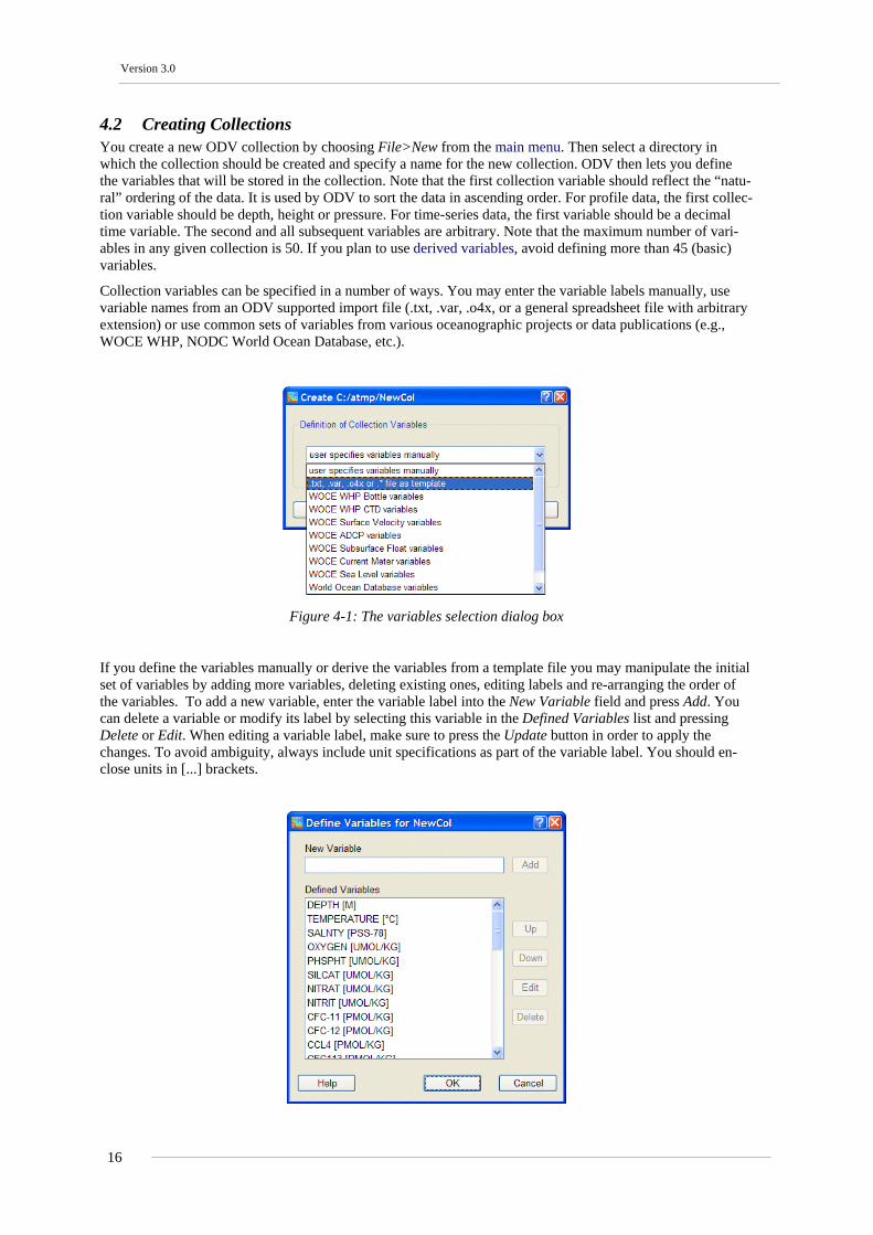
Collection variables can be specified in a number of ways. You may enter the variable labels manually, use variable names from an ODV supported import file (.txt, .var, .o4x, or a general spreadsheet file with arbitrary extension) or use common sets of variables from various oceanographic projects or data publications (e.g., WOCE WHP, NODC World Ocean Database, etc.).
Figure 4-1: The variables selection dialog box
If you define the variables manually or derive the variables from a template file you may manipulate the initial set of variables by adding more variables, deleting existing ones, editing labels and re-arranging the order of the variables. To add a new variable, enter the variable label into the New Variable field and press Add. You can delete a variable or modify its label by selecting this variable in the Defined Variables list and pressing Delete or Edit. When editing a variable label, make sure to press the Update button in order to apply the changes. To avoid ambiguity, always include unit specifications as part of the variable label. You should en-close units in [...] brackets.
16

Ocean Data View User’s Guide
Figure 4-2: The variables definition dialog box
You can use formatting control sequences in the variable labels to create subscripts, superscripts, and special symbols.
To complete the definition of variable labels press OK. ODV will create the collection; it will switch to STATION mode and draw a default, global map. Note that the collection is empty initially. You should use options from the Import menu to import data into the collection.
4.3 Collection Files Summary This section provides an overview over the various files that comprise an ODV collection. The information is for interested users and may be useful in case of problems or unexpected behavior. Normally, a user need not be concerned with the collection file structure.
ODV stores the information about collection variables, stations and the actual data values in separate files (.var, .hob and .dob, respectively). cfg files don't contain data values per se, but store configuration settings that define the way the user "looks" at the data in a collection. Configuration settings include items such as map domain, station selection criteria, window-layout and many other parameters. The required .var, .hob and .dob files of a collection must all be located in the same directory. cfg files may be stored anywhere on the disk. Note that you should not edit any of the collection files manually.
Table 4-2: Summary of ODV collection files Extension Format Comment Basic files Must be present. <col>.var ASCII Defines collection variables, stores collection name and number of stations. On
Windows this file type is automatically associated with the ODV executable, e.g. double-clicking on the .var file starts ODV and opens the respective collection.
<col>.hob binary Stores the station meta-data (name, position, date, etc.). <col>.dob binary Stores the actual station data and quality flags. Info File Optional <col>.info ASCII Description of the collection (in freeform text format). ODV automatically cre-
ates an .info file containing information on dimensions and variables, when open-ing a netCDF file.
Auxiliary Files If not present, ODV automatically creates these files. <col>.inv ASCII Collection inventory listing by cruises. <col>.cid binary Cruise ID numbers <col>.log ASCII Collection log file. Keeps records of data changes. <col>.idv ASCII Lists IDs of key variables used as input for derived variables (depth, temperature,
oxygen, etc.) <col>.cfl ASCII Contains names of most recently used configuration file and output directory. <col> above represents the collection name. Note that all files must be located in the same directory (collection directory).
Table 4-3: Summary of ODV configuration files Extension Format Comment <any>.cfg binary Configuration files storing layout, value ranges, derived and iso-surface variable
selections, and many other settings. The name of the collection that owns a con-figuration is recorded inside the cfg file. Certain restrictions apply, if a different collection uses the cfg file.
<any>.sec ASCII Stores section outlines and characteristics.
17
Version 3.0
File names are arbitrary (indicated as <any> above). Cfg and sec files may be located in any directory.
4.4 Migrating Between Windows, UNIX and Mac OS X Data collections and configuration files produced with the ODV multi-platform software are platform inde-pendent and can be used on all supported systems without modification. Data collections and configuration files produced with the ODV versions 4.0 or higher for Windows and Solaris are also supported by the ODV multi-platform software.
18
Ocean Data View User’s Guide
5 Importing Data
5.1 ODV Spreadsheet Files ODV can read and import data from a variety of spreadsheet-type ASCII files. If the format of the import file is generic ODV spreadsheet format compliant, the data import will be fully automatic and no user interaction is required. Generic ODV spreadsheet files can be dropped on the ODV window or icon. Other spreadsheet data files can be read and imported as well, if they satisfy the general ODV spreadsheet format requirements. The import of general ODV spreadsheet files usually requires user interaction. ODV will prompt for informa-tion about the specific file format and will ask the user to identify specific meta-data and data columns.
ODV supports spreadsheet data files with or without station meta-data information and with or without column label information. ODV spreadsheet files may contain comments. The column separation character may be one of the following: TAB, semicolon (;), comma (,), SPACE, or slash (/). The missing data indicator value(s) may be a list of arbitrary numerical value(s) or a blank field. Multiple values must be separated by one or more spaces. Fields in the import file that are empty or contain one of these values or are considered missing.
ODV generic and general spreadsheet files may contain data for many stations from many cruises. All samples of a given station must be in consecutive order but need not necessarily be sorted. When reading the file, ODV breaks the data into stations whenever one or more of the entries for Cruise, Station, and Type change from one line to the next. If Station is not provided in the data file, the date mon/day/yr and the Longitude [de-grees_east] and Latitude [degrees_north] values are checked, and a station break occurs whenever one or more of these values change. The imported data from these files are added to the currently open data collec-tions, or, if no collection is currently open, are used to create a new collection.
To import data from a generic ODV spreadsheet file into the currently open collection choose Import>ODV Spreadsheet and use the standard file-select dialog to identify the data file that you want to import. Specify import options and press OK to start the data import. Generic ODV spreadsheet files can also be dragged-and-dropped onto the ODV icon or an open ODV window.
To import data from a general ODV spreadsheet file into the currently open collection choose Import>ODV Spreadsheet and use the standard file-select dialog to identify the data file that you want to import. If the file format deviates from the generic ODV spreadsheet format, a Spreadsheet File Properties dialog box appears and lets you specify the column separation character and the missing data value(s) (multiple values must be separated by one or more spaces; fields that are empty or contain one of these values or are considered miss-ing). You can also identify the line containing the column labels (leave empty if not present) and the first data line. ODV provides reasonable defaults for all items and only a few changes should be necessary in most cases. For the Column Sep. Character choose the character that will give a vertical list of labels in the Column Labels box. Press OK when all spreadsheet file properties are set, or press Cancel to abort the import.
If the labels for the metadata columns deviate from the specifications of the generic ODV spreadsheet format (see below), a Header Variable Association dialog box appears that lets you associate input columns with the collection metadata variables, or it lets you set defaults for those variables not provided in the input file. Al-ready associated variables are marked by asterisks (*). To define a new association select items in the Source File and Target Collection lists and press Associate. To invoke a conversion during import press Convert and choose one of the available conversion algorithms. To delete an existing association, select the respective variables and press Undo. If the import file does not contain information for one or more collection header variables you can specify defaults: (1) select the respective target variable; (2) press Set Default and (3) enter the default value. Note that the specified default settings are used for all data lines in the file. Press OK when done or Cancel to abort the import procedure. Finally specify import options and press OK to start the data import.
5.2 WOCE Hydrographic Data You can use ODV to import original hydrographic data in WHP exchange format into existing or new data collections. WHP exchange format data files can be found at the WHP DAC (http://whpo.ucsd.edu/) or on the final WOCE data release on DVD-ROM. To import the data into an existing collection, open the collection. To import into a new collection, create the collection and make sure you choose either WOCE WHP Bottle vari-ables or WOCE WHP CTD variables when defining the variables to be stored in the collection.
To import WHP exchange format bottle data into the currently open collection choose Import>WOCE WHP Bottle (exchange format)>Single File from ODV’s main menu. Use the standard file-selection dialog to select the WHP data set. Note that the default extension of WHP exchange files is .csv. If your data file has a differ-
19

Version 3.0
ent extension, choose file-type All Files in the file-selection dialog. Then specify import options and press OK to start the data import. ODV will read and import all stations in the data file. ODV identifies and imports the WOCE data quality flags in addition to the actual data values. These quality flags can later be used to filter the data by excluding, for instance, bad or questionable data from the analysis. You can modify the data quality filter by choosing selection criteria from the map popup menu (choose the Sample Selection tab).
To import CTD data into the currently open collection, choose Import>WOCE WHP CTD (exchange for-mat)>Single File from ODV’s main menu and select the .zip file that contains the CTD data to be imported. Then specify vertical sub-sampling parameters or keep the default setting, which is no sub-sampling. ODV will then unpack the .zip file and import all CTD stations into the currently open collection.
You can import data from multiple WHP exchange files in a single import operation. In such a case the same import options are used for all files imported during the operation. For multi-file data import you have to pre-pare a ASCII file with default extension .lst that contains the names of the files to be imported. Use full path-names, and specify one file name per line. Then choose either Import>WOCE WHP Bottle (exchange for-mat)>Multiple Files or Import>WOCE WHP CTD (exchange format)>Multiple Files, specify import options and press OK to start the data import.
Note that ODV can handle up to 20,000 samples per station. If a CTD station contains more samples, it will be truncated. Also note that ODV automatically converts pressure in the source files to depth in the collection. If you need pressure as a variable, activate the derived variable Pressure(Depth).
During import, ODV maps WHP or IGOSS quality flags found in the WOCE import files to corresponding ODV quality flags. For details of the quality flag mapping see the Appendix.
5.3 WOD Hydrographic Data You can use ODV to import original hydrographic data from the World Ocean Database (WOD) into existing or new data collections. The WOD data files can be imported directly from the WOD CD-ROMs or from on-line data files after download over the Internet. To import into an existing collection, open the collection. To import into a new collection, create the collection and make sure you choose World Ocean Database variables when defining the variables stored in the collection. To import WOD data into the currently open collection choose Import>World Ocean Database>Single File. Use the standard file selection dialog to identify a zipped .gz data file of the WOD data set to be imported. Choose file-type All Files (*.*) if you want to select a WOD file that is already unzipped. Specify station selection criteria to be satisfied by WOD stations or simply press OK to import all stations falling into the current map domain, specify import options and press OK to start the data import. ODV will read the selected WOD data file and import all stations that satisfy the station selection criteria. The cruise label of imported stations is constructed from the WOD identifier, e.g., ”WOD98”, “WOD01”, etc. followed by the two digit NODC country-code and the six digit OCL cruise number. The unique OCL profile number is used by ODV as station number. ODV recognizes and uses data quality flags found in the import files.
You can import data from multiple WOD files in a single import operation. In such a case the same station selection criteria and import options are used for all files imported during this operation. For multi-file data import you have to prepare a ASCII file with default extension .lst that contains the names of the files to be imported. Use full pathnames, and specify one file name per line. Then choose Import>World Ocean Data-base>Multiple Files, specify station selection criteria to be satisfied by WOD stations (simply press OK to import all stations falling into the current map domain), specify import options and press OK to start the data import. ODV will read all the files listed in the ASCII file and will import all stations that satisfy the station selection criteria.
Note that during WOD data import only stations falling into the current map domain are actually imported into the collection. To make sure that all stations are imported, choose Global Map from the map popup menu before starting the import.
During import, ODV maps WOD quality flags found in the import files to corresponding ODV quality flags. For details of the quality flag mapping see the Appendix.
5.4 WOA94 Hydrographic Data You can use ODV to import original hydrographic data directly from the distribution CDs of the World Ocean Atlas 1994 by choosing Import>World Ocean Atlas 94>Single File. Use the standard Windows file-select dialog to identify the data file (*.ol) of the WOA94 data set that you want to import. Specify station selection
20
Ocean Data View User’s Guide
criteria to be satisfied by WOA94 stations (simply press OK to import all stations falling into the current map domain), specify import options and press OK to start the data import. ODV will read the selected WOA94 data file and import all stations that satisfy the station selection criteria.
You can import data from multiple WOA94 files using the same station selection criteria and import options in a single import operation. To do so, prepare an ASCII file (default extension .lst) containing the names of the files to be imported (full pathnames, one per line). Choose Import>World Ocean Atlas 94>Multiple Files, specify station selection criteria to be satisfied by WOA94 stations (simply press OK to import all stations falling into the current map domain), specify import options and press OK to start the data import. ODV will read all the files listed in the ASCII file and will import all stations that satisfy the station selection criteria.
Note that only stations falling into the current map domain are imported into the collection. To make sure that all stations are imported, choose Global Map from the map pop-up menu before starting the import.
5.5 SD2 Hydrographic Data You can use ODV to import original hydrographic data from NODC SD2 files into existing or new data col-lections. To import into an existing collection, open the collection. To import into a new collection, create the collection and make sure you choose NODC SD2 variables when defining the variables stored in the collec-tion. To import SD2 data into the currently open collection choose Import>NODC SD2 Format>Single File. Use the standard file-selection dialog to identify the data file to be imported. Specify import options and press OK to start the data import.
If you want to import multiple SD2 files in one import operation, put all the SD2 files in a single directory and produce a file containing the list of SD2 file-names that you want to import (default list-file extension .lst; one file-name per line). Choose Import>NODC SD2 Format>Multiple Files and select the list-file.
5.6 Other Hydrographic Data In addition to ODV spreadsheet, WOCE WHP, World Ocean Database, World Ocean Atlas 1994 and SD2, ODV supports the import of data from a variety of other formats. These include the Java Ocean Atlas spread-sheet format as well as the netCDF formats of most WOCE data streams. To import data in one of these for-mats into the currently open collection select the appropriate option from the Import menu. Note that for many import routes there is a choice between single and multiple file import. For multiple file import you have to specify an ASCII file that contains the full pathnames of all files to be imported. For single file import you have to specify the file that contains the data to be imported. All import routes require that the user specifies appropriate import options. During import, ODV maps data quality flags found in the import files to corre-sponding ODV quality flags. For details of the quality flag mapping see the Appendix.
ODV also supports a wide variety of other spreadsheet formats, including simple three column files with XYZ data. For backwards compatibility ODV still supports the o4x and o3x exchange formats.
21

Version 3.0
5.7 Import Options Dialog
When importing data, ODV will present an Import Options dialog that lets you control the actions taken during data im-port.
Figure 5-1: The import options dialog box
Import Mode Add/Replace Station Data: Choose this option if you want to add data from the import file to the collec-tion. If the Check for Existing Stations box is checked, ODV searches the collection for stations with the same name, date and position and (if found) asks for permission to replace the existing station in the collection with the new version from the import file (see Cruise Label Association below for a descrip-tion of the station search procedure).
Merge Data (selected variables): Choose this option if you want to add data for one or more variables (merge variables) and leave existing data for other variables unchanged. A ”merged” value of a ”merge variable” at a given sample depends on existing and new variable values according to the following ta-ble: Existing value New value Merged value yes yes Average of existing and new values yes no Existing value no yes New value no no Missing value
Note that the Check for Existing Stations box cannot be unchecked for this mode. Before adding data, ODV searches the collection for matching stations (see Cruise Label Association below for a descrip-tion of the station search procedure) and if found, reads the original station from the collection, adds the data for the selected variables and replaces the original station with the updated version. If no matching station is found, the user is notified. Update Data (selected variables): Choose this option if you want to update data for one or more vari-ables (update variables) and leave existing data for other variables unchanged. An ”updated” value of an ”update variable” at a given sample only depends on the new variable values and existing values are discarded. Note that the Check for Existing Stations box cannot be unchecked for this mode. Before up-dating data, ODV searches the collection for matching stations (see Cruise Label Association below for a description of the station search procedure) and if found, reads the original station from the collection, updates the data for the selected variables and replaces the original station with the updated version. If no matching station is found, the user is notified.
22
Ocean Data View User’s Guide
Cruise Label Association When replacing or merging data, ODV first searches the target collection for an existing station that matches the given station to be imported. This search is made by comparing cruise name, station name, station type, longitude, latitude and date. For a successful match, all items except cruise name are re-quired to be identical. For cruise name you can establish alias names using the Target and Source combo-boxes. If, for instance, in the existing collection a set of stations is named 06MT15/3 and in the import file the same stations are named METEOR15/3 you can set up an alias name by first choosing 06MT15/3 from the Target combo-box and then typing METEOR15/3 in the source field. Note that the default entries in the Source field are the same as the target names, so in case the cruise labels in the import file and in the collection are identical, you do not need to modify the Cruise Label Association at all.
Variable Association Usually the number, order and meaning of variables stored in the import file differ from the number, order and meaning of variables stored in the collection. Therefore you must establish a source/target as-sociation of variables. ODV automatically associates variables with matching labels (name and units). Note that associated variables are marked with a *. You can click on such a variable to identify its as-sociated variable. To establish a variable association manually click on the respective source variable, then click on the target variable to be associated with the source variable and either press the Associate or Convert but-tons. Use Associate if the data values in the import file should be imported without modification, but use Convert if you need to transform units during import. When using Convert, you can choose be-tween predefined, commonly used transformations and you can establish your own general linear trans-formation formula. For ODV Spreadsheet imports you can set default values for target variables for which no correspond-ing source variable is provided in the import file. This is useful, for instance, if you import longi-tude/latitude maps of some quantity Z from ASCII files containing three columns X/Y/Z, but not con-taining data for the specific surface or depth level. To set a default value for a target value, first select a the variable in the Target Collection list, then press the Use Default button and enter the desired default value for this target variable. Note that this target variables is now marked with a + sign. The specified value will be used for every sample of every station imported during this operation. Source variables not associated with a target variable will not be imported into the collection. If you merge data into the collection, establish associations only for those variables that you want to add to the collection. Note that the first variable in any ODV collection must be associated in any case.
23
Version 3.0
6 Exporting Data
6.1 Spreadsheet Files You can export the data of the currently selected stations into a single ASCII ODV spreadsheet file by choos-ing Export>ODV Spreadsheet from ODV's main menu. Then select the variables to be included in the export file (default: all variables) and specify destination directory and file-name using the standard file-select dialog-box. Note that spreadsheet files can be re-imported using the Import>ODV Spreadsheet. Note that valid ODV spreadsheet file names may not contain spaces or any of the following characters: \ / :.
6.2 ODV Collection You can export the data of the currently selected stations into a new ODV collection by choosing Ex-port>ODV Collection from ODV's main menu. Then select the variables to be included in the new collection (default: all variables) and specify destination directory and file-name using the standard file-select dialog-box. Note that valid ODV collection names may not contain spaces or any of the following characters: \ / :.
6.3 ASCII Listings You can export the data of the currently selected stations into a single ASCII listing file by choosing Ex-port>ODV4.x Listing from ODV's main menu. Then select the variables to be included in the export file (de-fault: all variables) and specify destination directory and file-name using the standard Windows file-select dialog-box. Note that ODV4.x Listing files can be re-imported using the Import> ODV4.x Listing. For further information on the ODV4.x Listing format click here. Note that valid ODV listing names may not contain spaces or any of the following characters: \ / :.
6.4 Exporting X/Y/Z Plot Data You can export the data values displayed in ODV plot windows to ASCII files for subsequent processing (av-eraging, gridding, contouring, etc.) by choosing Export>X/Y/Z Data from ODV’s main menu. Enter a descrip-tive text identifying the data of this export (txtID) and click OK. ODV will create a sub-directory in the local ODV directory (normally <home>\odv_local) named export\txtID. All exported files will be written to this directory. If it already exists, ODV asks for your permission to delete all files from the directory before con-tinuing. Note that the names of the exported files start with “win?” where ? represents the respective window number. The actual x-y-z-sigma_z data are found in files win?.oai (one data point per line).
For windows with gridded fields, ODV also exports the results of the gridding operation (files win?.oao). The format of the .oao files is as follows:
0 (ignore)
nx ny (no of x and y grid-points)
... nx X-grid values ... (X-grid positions)
... ny Y-grid values ... (Y-grid positions)
... nx*ny gridded values ... (estimated field, X-line by X-line starting at first Y-grid value)
... nx*ny gridded values ... (estimation quality, X-line by X-line starting at first Y-grid value)
6.5 Exporting Reference Datasets You can save the original data of the current plot windows in ASCII files and use these data later as reference datasets by choosing Export>X/Y/Z Data as Reference from ODV’s main menu. Enter a descriptive text iden-tifying the reference data (txtID) and click OK. ODV will create a sub-directory in the local ODV directory (normally <home>\odv_local) named reference\txtID and writes all files to this directory. If the directory al-ready exists, ODV asks for your permission to delete the current contents before continuing. Reference data are used by ODV for defining difference variables.
24

Ocean Data View User’s Guide
7 Derived Variables In addition to the basic variables stored in the collection files, ODV can calculate a large number of derived variables which (once defined) are available for analysis and use in the data plots in the same way as the basic variables. There are three types of derived variables:
• built-in derived variables including many commonly used parameters from physical and chemical oceanography.
• macro files of user defined expressions stored in files for use with arbitrary ODV collections.
• expressions defined by the user “on-the-fly” for the current collection only.
To define or delete derived variables choose the Derived Variables option from the canvas popup menu or Configuration>Derived Variables from the main menu. To add a macro choose Macro File from the “Choices” list; to add an user defined expression choose Expression. To add a built-in derived variable choose any other item in the “Choices” list.
7.1 Built-in Derived Variables Algorithms for many physical oceanographic parameters, such as potential temperature, potential density (rela-tive to arbitrary reference pressures), neutral density, Brunt-Väisälä Freq., and dynamic height, are built into the ODV software. In addition, various parameters of the carbon dioxide system in seawater, the saturation concentrations and partial pressures of many gases and many other variables from chemical oceanography are also available as easily selectable derived variables. Some useful mathematical expressions, such as the ratio of two arbitrary variables as well as vertical integrals and derivatives, are also available. A list of built-in de-rived variables is shown below. All these variables can be requested by the user, they are then calculated by ODV on-the-fly, and they can be analyzed and visualized in the same way as the basic variables stored in the collection files.
To define or delete built-in derived variables choose the Derived Variables option from the canvas popup menu. ODV will show list-boxes of available and already defined derived variables. To add a derived variable select an item from the Choices list and press Add. If you define a derived variable that needs additional in-formation for its definition (e.g., potential temperature and potential density require the reference pressure) you have to provide this information on dialog boxes that appear automatically. Many derived variables re-quire that you identify the appropriate input variable(s).
To delete a derived variable select this variable in the Already Defined list box and press Delete or simply double-click on the item to be deleted. Note that when deleting a variable that is required as input by other derived variables, these quantities are deleted as well. To edit ODV macros and expressions (for more infor-mation on these special derived variables see below) select the respective variable in the Already Defined list box and press Edit.
Table 7-1: List of built-in derived variables Variable Comment AOU [µmol/kg] Apparent oxygen utilization Brunt-Väisälä Freq. [cycl/h] EOS80 CFC-11 Saturation [%] Warner & Weiss, Deep Sea Res., 32,1485-1497,1985 CFC-12 Saturation [%] Warner & Weiss, Deep Sea Res., 32,1485-1497,1985 CFC-10 Saturation [%] Bullister & Wisegarver, Deep Sea Res., 45,1285-1302,1998 CFC-113 Saturation [%] Bu & Warner, Deep Sea Res., 42,1151-1161,1995 CH4 Saturation [%] Wiesenburg & Guinasso, J. Chem. Eng. Data,24,356-,1979 CO*
2(TCO2,TALK) [µmol/kg] (details) CO3
2-(TCO2,TALK) [µmol/kg] (details) Day of Month(header mon/day/year) Day of the Month derived from header mon/day/year Day of Month (time variable) Day of the Month derived from a time variable Day of Year(header mon/day/year) [days] Day of the Year [days] derived from header mon/day/year Day of Year(time variable) [days] Day of the Year [days] derived from a time variable Difference from Reference Data (details) Dynamic Height [dyn m] EOS80 (any reference pressure) fCO2(TCO2,TALK) [µAtm] (details) Freezing Temperature [°C] F. Millero, UNESCO Tech. Papers in the Marine Science, No. 28., 29-35, 1978 HCO3
-(TCO2,TALK) [µmol/kg] (details) Latitude Decimal latitude derived from station header
25

Version 3.0
Longitude Decimal longitude derived from station header Month of Year(header mon/day/year) Month of Year derived from header mon/day/year Month of Year(time variable) Month of Year derived from a time variable Neutral Density [kg/m3] Jackett & McDougall, J. Phys. Ocean., 237-263, 1997 (more) OmegaA(TCO2,TALK) (details) OmegaC(TCO2,TALK) (details) Oxygen Saturation [%] Weiss, Deep Sea Res., 17, 721-735, 1970 pCFC-11 [pptv] Warner & Weiss, Deep Sea Res., 32,1485-1497,1985 pCFC-12 [pptv] Warner & Weiss, Deep Sea Res., 32,1485-1497,1985 pCFC-10 [pptv] Bullister & Wisegarver, Deep Sea Res., 45,1285-1302,1998 pCFC-113 [pptv] Bu & Warner, Deep Sea Res., 42,1151-1161,1995 pCH4 [ppbv] Wiesenburg & Guinasso, J. Chem. Eng. Data,24,356-,1979 pCO2(TCO2,TALK) [µAtm] (details) pHtot(TCO2,TALK) (details) Potential Density [kg/m3] EOS80 (any reference pressure) Potential Temperature [°C] Bryden, Deep Sea Res.,20,401-408, 1973 (any reference pressure) Potential Vorticity [10-12 m-1 s-1] Planetary potential vorticity (derived from Brunt Vaissala Frequency Q=f/g*N2) Pressure [db] Saunders, J. Phys. Ocean., 1981 Quality Flag Any variable Ratio Any two variables Revelle Factor(TCO2,TALK) (d fCO2 / d TCO2) / (fCO2 / TCO2). (details) Sound Speed [m/s] Fofonoff & Millard, Unesco Tech. Pap. in Mar. Sci._, No. 44, 53 pp, 1983 Specific Heat Cp [J/(kg °C)] F. Millero et al, J. Geoph. Res., 78, 4499-4507, 1973 Time(header mon/day/year) [yr] Decimal time [yr] derived from header mon/day/year Time(time variable) [yr] Decimal time [yr] derived from a time variable Vertical Derivative Any variable Second Vertical Derivative Any variable Vertical Integral Any variable Year(header mon/day/year) Year derived from header mon/day/year Year(time variable) Year derived from a time variable
Parameters of the carbon dioxide system in sea water The following parameters of the carbon dioxide system in sea water are provided as derived variables:
1. pH (total scale), 2. fugacity and partial pressure of CO2 (fCO2 and pCO2 ), 3. concentrations of CO*
2, CO32-, and HCO3
-, 4. Revelle, or homogeneous buffer, factor, 5. solubility ratios [CO3
2-]*[Ca2+] / Ksp for calcite and aragonite, OmegaC and OmegaA. All these quantities are calculated as functions of in-situ depth (or pressure), temperature, salinity, total inor-ganic carbon (TCO2), total alkalinity (TALK), phosphate and silicate. If phosphate and/or silicate data are not available, concentration values of zero are assumed. ODV uses the alkalinity definition of Dickson (1981) and treats all terms except HS, S and NH3. pH is calculated using an iterative Newton method.
The choice of equilibrium constants follows the summary of Dickson&Goyet (1994): K1, K2 are from Roy et al. (1993), K0 is from Weiss (1974), KB is from Dickson (1990), KS is from Dickson (1990), KF is from Dick-son&Riley (1979), KW is from Millero (1995), K1p, K2p, K3p and KSi are from Millero (1995), and the solubility products Ksp of calcite and aragonite are from Mucci (1983). The pressure dependence of the equilibrium con-stants is from Millero (1995). Typographical errors in various publications (as summarized in Lewis&Wallace (1998)) are considered.
The carbon chemistry implementation in ODV (versions 2.1 and later) has been checked by comparing with other, independent software output, and the results have been found to be in very good agreement with values from the CO2SYS.EXE application of Lewis&Wallace (1998). Note that previous ODV versions calculated "potential" pH and carbon system parameters, e.g., the values a water parcel would have if raised to the surface adiabatically. These values are different from the in-situ values obtained by ODV versions 2.1 and later. DOE (U.S. Department of Energy). 1994. Handbook of methods for the analysis of the various parameters of the carbon dioxide system in sea water. Version 2. ORNL/CDIAC-74. A. G. Dickson and C. Goyet (eds.), Carbon Dioxide Information Analysis Center, Oak Ridge National Laboratory, Oak Ridge, Tenn.
Lewis, E., and D. W. R. Wallace. 1998. Program Developed for CO2 System Calculations. ORNL/CDIAC-105. Carbon Dioxide Informa-tion Analysis Center, Oak Ridge National Laboratory, U.S. Department of Energy, Oak Ridge, Tennessee.
26

Ocean Data View User’s Guide
Usage of Vertical Integral The user first selects the variable for which the vertical integral is to be calculated (designated A in the follow-ing; any basic or already defined derived variable can be used) and specifies the starting depth z0 for the inte-gral (default: 0 m). For each sample of a given station, ODV will calculate the integral A*dz from z0 to the respective level. The units of the integral are the units of the quantity A times length (km used by ODV). For variables with volumetric concentration units (e.g., moles per cubic meter) the calculated integral is equivalent to "standing stock per square meters". Note that by definition the value of the integral at z0 is zero. (Example: To obtain the salt content in the top 500 m of the water column, select salinity as variable for the integral and use 0 as start value. Then look up the value of the vertical integral at 500 m (by interpolating between neighboring points) or in SURFACE mode define the integral at depth=500 as an iso-surface variable.)
7.2 Derived Variable Macros You can implement new derived variables not included in the list of built-in derived quantities provided that the value of your new derived variable for a specific sample only depends on other variable values of the same sample. In these cases you specify the input variables and the formula of the new derived quantity in a macro file. Macro files must have the extension .mac, they must be located in the ODV macros directory (<home>\odv_local\macros) and their format must follow the specifications given below. You can use the ODV Macro Editor (invoked by: Utilities>Invoke Macro Editor) to facilitate macro definition. Use the exam-ple macro files that are distributed with ODV as sample files for your own definitions.
You activate a macro derived variable by selecting Derived Variables from the canvas popup menu and choos-ing Macro File from the list of available quantities. Then select one of the macro files found in the ODV mac-ros directory <home>\odv_local\macros and identify the variables needed to calculate the new quantity. If one of the required variables is not available, press Not Available to abort setup of the macro file.
7.2.1 Macro Editor
You can create and edit Ocean Data View macro files using the Utilities>Invoke Macro Editor option. Select an existing macro file or choose a new macro name and define the macro following the instructions below. When done press OK and specify a name for the macro.
Macro Variable Label: Enter the label and units of the macro variable. Note that you can use various formatting
control sequences.
Format: Enter numeric format for ODV text-window: field-length and number of decimals.
Comments Enter one or more lines of comments describing the macro variable.
Input Variables List of input variables needed for the macro variable. To add an input variable, enter it’s label and units into the New field and press the << button (note that you can use the formatting sequences listed above). To delete a defined input variable, select it in the Defined list-box and press the >> button. Note that an ODV macro can have a maximum of nine input variables.
Expression In the Expression field you specify the operations to be performed when calculating the macro variable. You can use the operators + - * / ** for the basic arithmetic operations, sqrt for the square root, min and max for minimum and maximum of preceding two operands, ln and exp for the natural logarithm and exponential, sin and cos for sine and cosine (arguments in radians), and abs for the absolute value, respectively. Type in the macro formula using Reverse Polish Notation (operands precede operators; e.g., Hewlett-Packard calculator-style) and use, for instance, the sequence #1 to reference the value of input variable #1.
Use the symbols %H, %t, %d, %x, and %y to refer to topographic height at the station position (given in me-ters; positive for land and negative for ocean), time of observation (in years since 1900; e.g., %t=84.4877 for Jun/27/84), day-of-the-year, (east-) longitude and (north-) latitude, respectively. Note that the topographic height %H is only available if you have installed one of the GEBCO1 or ETOPO2 optional packages.
You can store intermediate results in internal variables %0, %1, …, %9 using operators =%0, =%1, …, =%9. Stored values can be used later in the calculation by typing %0, %1, etc. Note that the =%n operators consume their operands, e.g., the respective value is taken off the stack. You must separate operands and operators by one or more spaces. Continue the definition of the macro expression on following lines, if necessary. Note that
27
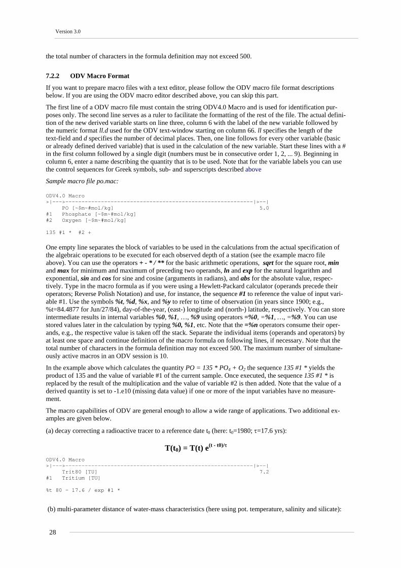
Version 3.0
the total number of characters in the formula definition may not exceed 500.
7.2.2 ODV Macro Format
If you want to prepare macro files with a text editor, please follow the ODV macro file format descriptions below. If you are using the ODV macro editor described above, you can skip this part.
The first line of a ODV macro file must contain the string ODV4.0 Macro and is used for identification pur-poses only. The second line serves as a ruler to facilitate the formatting of the rest of the file. The actual defini-tion of the new derived variable starts on line three, column 6 with the label of the new variable followed by the numeric format ll.d used for the ODV text-window starting on column 66. ll specifies the length of the text-field and d specifies the number of decimal places. Then, one line follows for every other variable (basic or already defined derived variable) that is used in the calculation of the new variable. Start these lines with a # in the first column followed by a single digit (numbers must be in consecutive order 1, 2, ... 9). Beginning in column 6, enter a name describing the quantity that is to be used. Note that for the variable labels you can use the control sequences for Greek symbols, sub- and superscripts described above
Sample macro file po.mac:
ODV4.0 Macro >|--->----------------------------------------------------------|>--| PO [~$m~#mol/kg] 5.0 #1 Phosphate [~$m~#mol/kg] #2 Oxygen [~$m~#mol/kg] 135 #1 * #2 + One empty line separates the block of variables to be used in the calculations from the actual specification of the algebraic operations to be executed for each observed depth of a station (see the example macro file above). You can use the operators + - * / ** for the basic arithmetic operations, sqrt for the square root, min and max for minimum and maximum of preceding two operands, ln and exp for the natural logarithm and exponential, sin and cos for sine and cosine (arguments in radians), and abs for the absolute value, respec-tively. Type in the macro formula as if you were using a Hewlett-Packard calculator (operands precede their operators; Reverse Polish Notation) and use, for instance, the sequence #1 to reference the value of input vari-able #1. Use the symbols %t, %d, %x, and %y to refer to time of observation (in years since 1900; e.g., %t=84.4877 for Jun/27/84), day-of-the-year, (east-) longitude and (north-) latitude, respectively. You can store intermediate results in internal variables %0, %1, …, %9 using operators =%0, =%1, …, =%9. You can use stored values later in the calculation by typing %0, %1, etc. Note that the =%n operators consume their oper-ands, e.g., the respective value is taken off the stack. Separate the individual items (operands and operators) by at least one space and continue definition of the macro formula on following lines, if necessary. Note that the total number of characters in the formula definition may not exceed 500. The maximum number of simultane-ously active macros in an ODV session is 10.
In the example above which calculates the quantity PO = 135 * PO4 + O2 the sequence 135 #1 * yields the product of 135 and the value of variable #1 of the current sample. Once executed, the sequence 135 #1 * is replaced by the result of the multiplication and the value of variable #2 is then added. Note that the value of a derived quantity is set to -1.e10 (missing data value) if one or more of the input variables have no measure-ment.
The macro capabilities of ODV are general enough to allow a wide range of applications. Two additional ex-amples are given below.
(a) decay correcting a radioactive tracer to a reference date t0 (here: t0=1980; τ=17.6 yrs):
T(t0) = T(t) e(t - t0)/τ
ODV4.0 Macro >|--->----------------------------------------------------------|>--| Trit80 [TU] 7.2 #1 Tritium [TU] %t 80 - 17.6 / exp #1 *
(b) multi-parameter distance of water-mass characteristics (here using pot. temperature, salinity and silicate):
28
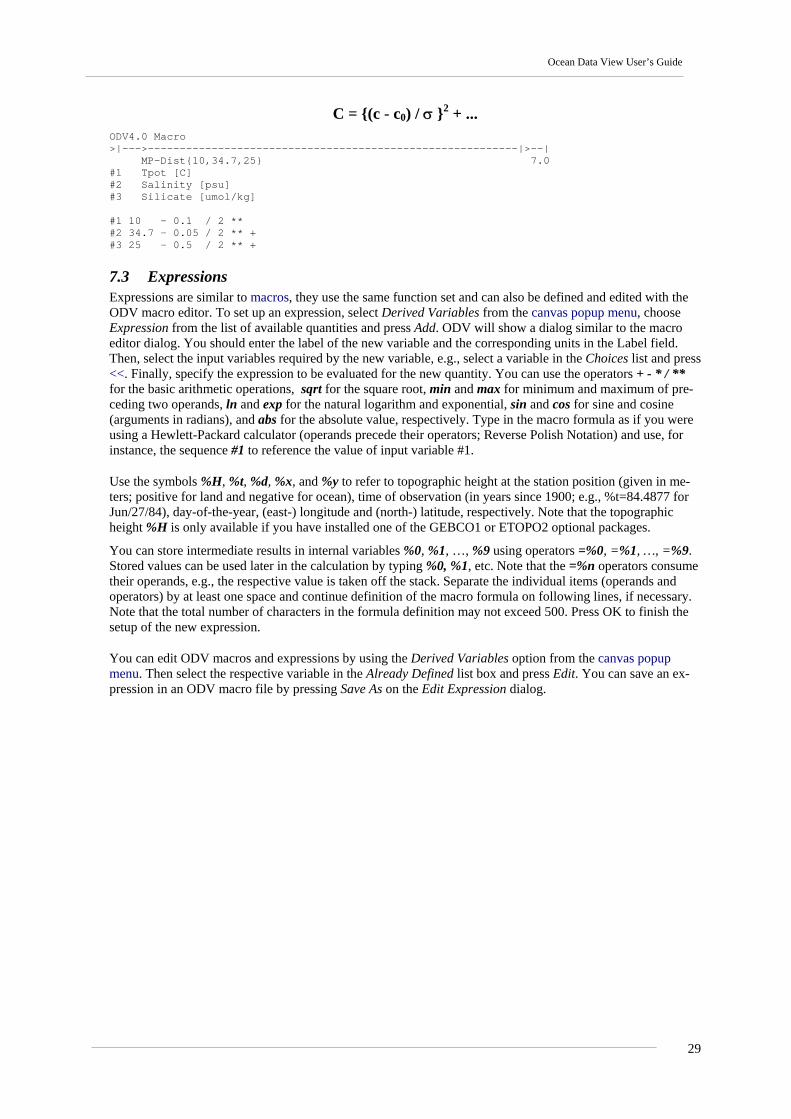
Ocean Data View User’s Guide
C = {(c - c0) / σ }2 + ... ODV4.0 Macro >|--->----------------------------------------------------------|>--| MP-Dist{10,34.7,25} 7.0 #1 Tpot [C] #2 Salinity [psu] #3 Silicate [umol/kg] #1 10 - 0.1 / 2 ** #2 34.7 - 0.05 / 2 ** + #3 25 - 0.5 / 2 ** +
7.3 Expressions Expressions are similar to macros, they use the same function set and can also be defined and edited with the ODV macro editor. To set up an expression, select Derived Variables from the canvas popup menu, choose Expression from the list of available quantities and press Add. ODV will show a dialog similar to the macro editor dialog. You should enter the label of the new variable and the corresponding units in the Label field. Then, select the input variables required by the new variable, e.g., select a variable in the Choices list and press <<. Finally, specify the expression to be evaluated for the new quantity. You can use the operators + - * / ** for the basic arithmetic operations, sqrt for the square root, min and max for minimum and maximum of pre-ceding two operands, ln and exp for the natural logarithm and exponential, sin and cos for sine and cosine (arguments in radians), and abs for the absolute value, respectively. Type in the macro formula as if you were using a Hewlett-Packard calculator (operands precede their operators; Reverse Polish Notation) and use, for instance, the sequence #1 to reference the value of input variable #1.
Use the symbols %H, %t, %d, %x, and %y to refer to topographic height at the station position (given in me-ters; positive for land and negative for ocean), time of observation (in years since 1900; e.g., %t=84.4877 for Jun/27/84), day-of-the-year, (east-) longitude and (north-) latitude, respectively. Note that the topographic height %H is only available if you have installed one of the GEBCO1 or ETOPO2 optional packages.
You can store intermediate results in internal variables %0, %1, …, %9 using operators =%0, =%1, …, =%9. Stored values can be used later in the calculation by typing %0, %1, etc. Note that the =%n operators consume their operands, e.g., the respective value is taken off the stack. Separate the individual items (operands and operators) by at least one space and continue definition of the macro formula on following lines, if necessary. Note that the total number of characters in the formula definition may not exceed 500. Press OK to finish the setup of the new expression.
You can edit ODV macros and expressions by using the Derived Variables option from the canvas popup menu. Then select the respective variable in the Already Defined list box and press Edit. You can save an ex-pression in an ODV macro file by pressing Save As on the Edit Expression dialog.
29

Version 3.0
Figure 7-1: The Edit Expression dialog box
30
Ocean Data View User’s Guide
8 Interactive Controls and ODV Modes
8.1 Choosing Current Sample and Current Station When a collection is open and ODV has drawn the station map, one of the valid stations in the map is the cur-rent station. This station is marked with a red cross, and the station meta-information is shown in the top line of the ODV text window. There are several ways to select a new current station:
(1) Click the left mouse button on any station in the map. If there are multiple stations at the same location and you want to select a particular one, hold down the SHFT key while clicking on the station posi-tion. This will produce a list of matching stations. Select the one which you want as current station and press OK. Without the SHFT key, the last matching station is selected by default.
(2) Choose Current Station by Name from the map popup menu and specific cruise label, station label and station type.
(3) Choose Current Station by Number from the map popup menu (or simply press #) and specify the in-ternal sequence number of the station.
(4) Press the right arrow key (->) to select the next valid station. (5) Press the left arrow key (<-) to select the previous valid station.
One of the samples of the current station is the current sample. The data values of the current sample are listed in line 3 of ODV’s text window. If data plots are on the screen the current sample is also marked by red cross hairs in each of the plots. In property/property plots, all data values of the current station are highlighted by a red line. The highlighting style can be changed using the Display Options dialog of the respective plot. High-lighting can also be switched off altogether.
You can select the next or previous sample of the same station by pressing the up/down and PgUp/PgDn ar-row-keys, or you can make any data point in any of the data plots the current sample by simply clicking on it with the left mouse button. Note that the information in the ODV text window is automatically updated when-ever you select a new current station or sample.
If you rest the mouse over the items in lines 2 and 3 of the text window, popup windows appear showing more detailed information on the data value, including its quality flag. You can change the numeric format and order in which the variables are listed in the text window by choosing Variables Settings from the text-window popup menu.
8.2 Changing Variable Settings For any collection variable you can modify its labels, the default min/max range, the numeric format and the position in line 3 of ODV’s text-window using the Variables Settings option of the text window popup menu (click right mouse button while over the text window and select Variables Settings).
First select a variable that you want to modify using the Variable control (if the mouse was over the respective variable when you right-clicked, this variable is already pre-selected). Then modify the different properties for this variable. You change the variable label and units string by editing the Label item. Note that the units should be enclosed between [ and ] brackets. You change the default lower and upper value ranges of the vari-able by setting the Minimum and Maximum entries. You modify the numeric format used to list data for the variable in line 3 of the text window by setting the Format entries. The first number specifies the length of the field (in characters) and the second number specifies the number of decimal places. Finally, you can change the position of the variable in the text window using the Position combo-box (select the new position of the variable, e.g. potential temperature next to (in-situ) temperature). Continue making changes for other variables (select them using the Variable combo-box) and press OK when you are done.
8.3 Changing Selection Criteria While drawing the station map, ODV checks every station in the collection and determines whether it satisfies the current station selection criteria. Only stations that pass this test are considered valid. Only these stations are marked in the map and only this station subset is available for subsequent browsing and plotting.
You can modify the station and sample selection criteria by using Selection Criteria from the map popup menu or Configuration>Selection Criteria from the main menu. Choose the category that you want to modify by clicking on the respective tab, e.g., Name/Range, Date/Time, Availability and Sample Selection, and modify
31
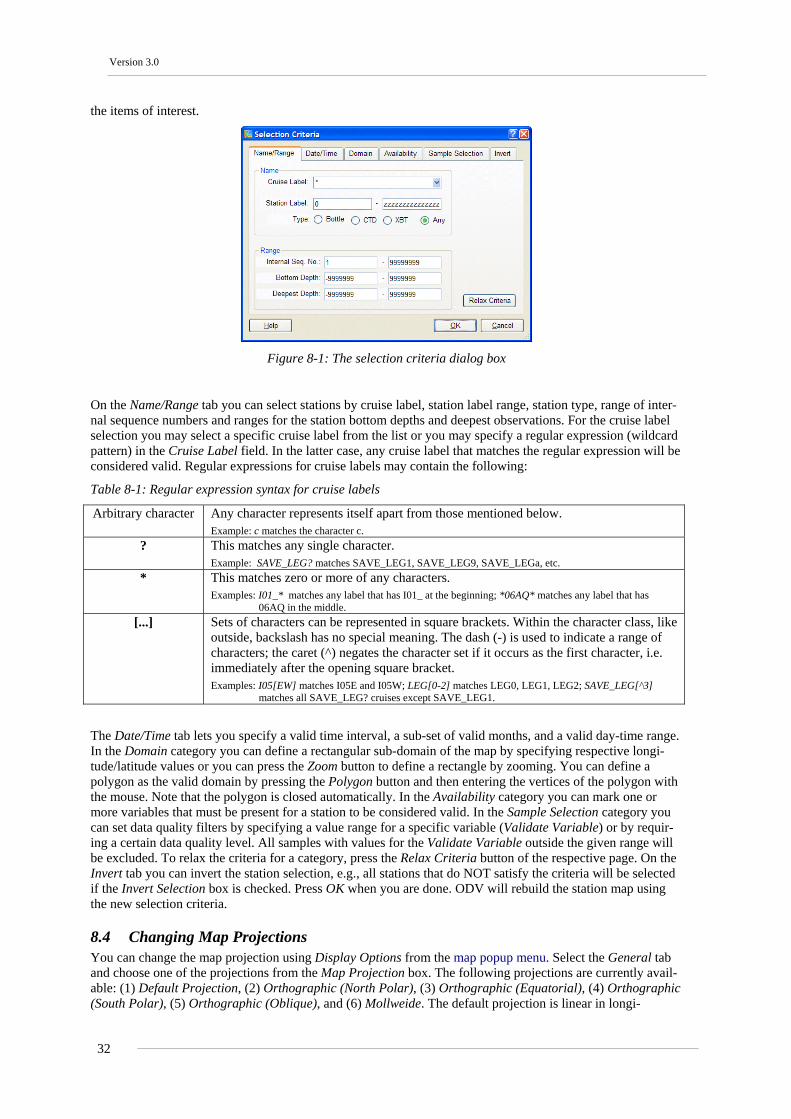
Version 3.0
the items of interest.
Figure 8-1: The selection criteria dialog box
On the Name/Range tab you can select stations by cruise label, station label range, station type, range of inter-nal sequence numbers and ranges for the station bottom depths and deepest observations. For the cruise label selection you may select a specific cruise label from the list or you may specify a regular expression (wildcard pattern) in the Cruise Label field. In the latter case, any cruise label that matches the regular expression will be considered valid. Regular expressions for cruise labels may contain the following:
Table 8-1: Regular expression syntax for cruise labels
Arbitrary character Any character represents itself apart from those mentioned below. Example: c matches the character c.
? This matches any single character. Example: SAVE_LEG? matches SAVE_LEG1, SAVE_LEG9, SAVE_LEGa, etc.
* This matches zero or more of any characters. Examples: I01_* matches any label that has I01_ at the beginning; *06AQ* matches any label that has
06AQ in the middle. [...] Sets of characters can be represented in square brackets. Within the character class, like
outside, backslash has no special meaning. The dash (-) is used to indicate a range of characters; the caret (^) negates the character set if it occurs as the first character, i.e. immediately after the opening square bracket. Examples: I05[EW] matches I05E and I05W; LEG[0-2] matches LEG0, LEG1, LEG2; SAVE_LEG[^3]
matches all SAVE_LEG? cruises except SAVE_LEG1.
The Date/Time tab lets you specify a valid time interval, a sub-set of valid months, and a valid day-time range. In the Domain category you can define a rectangular sub-domain of the map by specifying respective longi-tude/latitude values or you can press the Zoom button to define a rectangle by zooming. You can define a polygon as the valid domain by pressing the Polygon button and then entering the vertices of the polygon with the mouse. Note that the polygon is closed automatically. In the Availability category you can mark one or more variables that must be present for a station to be considered valid. In the Sample Selection category you can set data quality filters by specifying a value range for a specific variable (Validate Variable) or by requir-ing a certain data quality level. All samples with values for the Validate Variable outside the given range will be excluded. To relax the criteria for a category, press the Relax Criteria button of the respective page. On the Invert tab you can invert the station selection, e.g., all stations that do NOT satisfy the criteria will be selected if the Invert Selection box is checked. Press OK when you are done. ODV will rebuild the station map using the new selection criteria.
8.4 Changing Map Projections You can change the map projection using Display Options from the map popup menu. Select the General tab and choose one of the projections from the Map Projection box. The following projections are currently avail-able: (1) Default Projection, (2) Orthographic (North Polar), (3) Orthographic (Equatorial), (4) Orthographic (South Polar), (5) Orthographic (Oblique), and (6) Mollweide. The default projection is linear in longi-
32
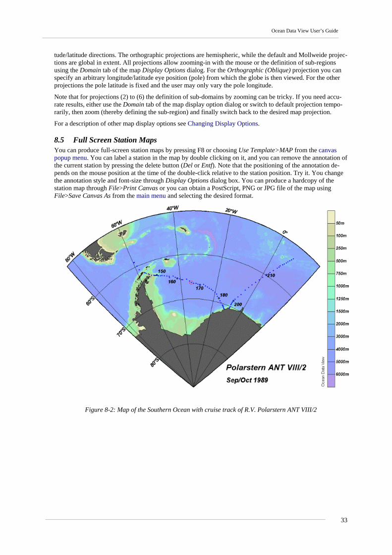
Ocean Data View User’s Guide
tude/latitude directions. The orthographic projections are hemispheric, while the default and Mollweide projec-tions are global in extent. All projections allow zooming-in with the mouse or the definition of sub-regions using the Domain tab of the map Display Options dialog. For the Orthographic (Oblique) projection you can specify an arbitrary longitude/latitude eye position (pole) from which the globe is then viewed. For the other projections the pole latitude is fixed and the user may only vary the pole longitude.
Note that for projections (2) to (6) the definition of sub-domains by zooming can be tricky. If you need accu-rate results, either use the Domain tab of the map display option dialog or switch to default projection tempo-rarily, then zoom (thereby defining the sub-region) and finally switch back to the desired map projection.
For a description of other map display options see Changing Display Options.
8.5 Full Screen Station Maps You can produce full-screen station maps by pressing F8 or choosing Use Template>MAP from the canvas popup menu. You can label a station in the map by double clicking on it, and you can remove the annotation of the current station by pressing the delete button (Del or Entf). Note that the positioning of the annotation de-pends on the mouse position at the time of the double-click relative to the station position. Try it. You change the annotation style and font-size through Display Options dialog box. You can produce a hardcopy of the station map through File>Print Canvas or you can obtain a PostScript, PNG or JPG file of the map using File>Save Canvas As from the main menu and selecting the desired format.
Figure 8-2: Map of the Southern Ocean with cruise track of R.V. Polarstern ANT VIII/2
33

Version 3.0
8.6 Property-Property Plots When ODV is in STATION mode (indicated in the lower right corner of the window; switch to STATION mode by pressing F9 or choosing one of the predefined STATION templates via Use Template>… from the canvas popup menu) you can produce property/property plots of the current station by pressing p or by double-clicking the left mouse on the current station in the map. You can add the data of other stations to the plots by either double-clicking on them or by selecting them as current station and pressing p. To delete one of the selected stations from the plots, make it the current station (for instance, by clicking on one of its data points in one of the plots) and press the delete key (Del or Entf , etc.). To clear the screen press Ctrl-X and to clear the list of selected stations press Ctrl-X twice.
See also: zooming and auto-scaling; selecting new X-and Y-variables; changing display options; printing; PostScript file.
Figure 8-3: Property-property plots of five selected stations from the South Atlantic Ventilation Experiment
(SAVE)
8.7 Zooming and Automatic Scaling You can change the variable ranges of any data plot by moving the mouse over this window, clicking the right mouse button to invoke the data plot popup menu and choosing either Full Range or Zoom. For Full Range, the X- and Y-Ranges of the current window are adjusted to accommodate all plotted data values in this win-dow. If you use Full Range (All) you can auto-scale all data plots on the screen.
If you select Zoom, a red zoom-frame appears around the current window. To manipulate this zoom-frame move the mouse over it, press the left mouse button and drag the frame to desired locations. To accept the current setting of the zoom-frame and adjust the variable ranges accordingly double-click the left mouse but-ton or press ENTER. If you want to abort the zoom operation and keep the present variable ranges, press ESC or click the right mouse button.
In addition to this the standard zoom procedure that allows maximum control, a "quick-zoom" option is also
34
Ocean Data View User’s Guide
available. When the mouse is over the map or any data plot press (and hold down) the Ctrl key (on Macintosh systems use the Apple key) and press (and hold down) the left mouse button to drag a zoom box. Releasing the left mouse button applies the zoom box settings to the window from which the “quick-zoom” was initiated.
8.8 Changing Window Layout ODV keeps window layout information separately for each of its modes (STATION, SCATTER, SECTION and SURFACE). The layout information includes position and size of map and data-plots, number of data-plots, variables on X-, Y- and Z-axis, size of symbols and the selection of topography files for the map. In each of its modes, you can change the respective window layout by invoking the canvas popup menu (click the right mouse button while over the canvas area) and choosing Window Layout. ODV will outline the current layout and lets you move, resize, delete or create windows. To perform one of these operations on a window, move the mouse inside that window and invoke the layout-popup menu by clicking the right mouse button and select the appropriate option.
If you choose Move/Resize a red zoom-frame appears around the respective window. You move and resize this zoom frame by moving the mouse over it, pressing the left mouse button and dragging. To accept the new size and position for the window double-click the left mouse button or press ENTER. To abort the Move/Resize operation leaving the window position unchanged press ESC. Note that overlay windows (see below) can not be moved or resized.
You create new windows by moving the mouse over one of the existing windows, right-clicking and choosing option Create New Window or Create Overlay Window. In both cases the initial properties of the new window are derived from the existing one. If you use Create New Window, the new window will be placed in the mid-dle of the ODV graphics canvas and you have to position and resize it using the Move/Resize option described above. If you use Create Overlay Window, some properties required for overlay windows will be set automati-cally, and the new window will be properly aligned with the existing one. You modify the properties of a new window after leaving Window Layout mode and invoking the Display Options dialog of the respective win-dow.
To select new variables on X-, Y- and Z-axis of a given window, select the appropriate option and choose a variable from the list-box that appears. Note that by default variable values increase to the right and upwards. If you want to reverse the direction (e.g., depth in depth profiles) check the Reverse Range box. Press OK to accept the choice.
You leave Window Layout mode by choosing either Accept or Cancel. Note that you can modify other proper-ties of map and data plots using the Display Options function from the map and data-plot popup menus.
8.9 Changing Display Options You can modify display properties of the map and any data plot using the Display Options function from the map and data-plot popup menus. To invoke these menus move the mouse over the respective window and click the right mouse button. Note that for overlay windows (two or more windows stacked on top of each other) this method gives you access to the top-most window only. In those cases use Configuration>Window Properties>… to change the properties of any particular window.
8.9.1 Map
The Map Display Options dialog lets you modify map properties from four categories: General, Layers, Do-main and Annotations. You access any of these categories by clicking on the respective tab. Detailed descrip-tions follow below.
35

Version 3.0
Figure 8-4: The display options dialog box of the map
General Select the color palette used for the map, choose a background color and specify whether grid lines should be drawn or not. Specify a map projection and choose color and symbol size for the station dots. Choose (auto-matic) for Station Dots’ Color to obtain different colors for different cruise labels.
Layers ODV can draw ocean bathymetry, coastlines, land topography and other, additional features like lakes, rivers, borders, sea-ice extend, ocean fronts etc. into the map window. For a sample .gif figure of a map with many layers see the samples directory of your ODV installation. A low resolution, global version of these geographi-cal feature files (GlobLR series) is provided by default when you install ODV. Higher resolution global and regional datasets are available as optional packages and can be downloaded and installed at any time. Choose one of the installed series from the Series list. Check the Draw Color Bar box if a bathymetry/topography color bar should be drawn.
The geographical features mentioned above are implemented and drawn by ODV as individual layers. These layers are grouped into seven layer sets: (1) pre-Bathymetry, (2) Ocean Bathymetry, (3) pre-Coastlines, (4) Coastlines, (5) pre-Topography, (6) Land Topography, (7) post-Topography. You compose a layer set by selecting it in the Layer Sets list and pressing the Compose button. ODV will show a list of available layers for this layer set. Choose one or more layers from the Available list (using standard single or multi-selection tech-niques), specify drawing characteristics and press the << button to add the layers to the Selected list. To re-move layers from the Selected list, select them and press >>.
When specifying drawing characteristics follow these rules:
(a) if the features should be outlined by lines (stroked), choose the appropriate line-width, -type and –color or choose none as color, if you don’t want outlines. Note that due to limitations of Windows, lines that are more than 1 pixel wide, will always be solid on the screen and in PNG and JPG files. ODV PostScript files, however, honor your selection for any line-width.
(b) if the features should be filled, choose the appropriate Fill color or none, if you don’t want filling.
If you choose automatic for line and fill colors, ODV will use default colors. Note that for some layer sets automatic defaults to none. Also note that some feature files like rivers or borders should not be filled, and you should explicitly set the fill color to none.
When ODV produces the map it processes the layer sets in the order given above. For a given layer set it draws the individual layers in the order in which they appear in the Selected list (note that ocean bathymetry and land topography layers are sorted automatically when you add them). You should define sea-ice distribu-tions in the pre-Coastlines set and lakes, rivers and borders in the post-Topography category.
Domain Specify a longitude/latitude sub-domain or switch to the full domain of the collection or to a global map.
36
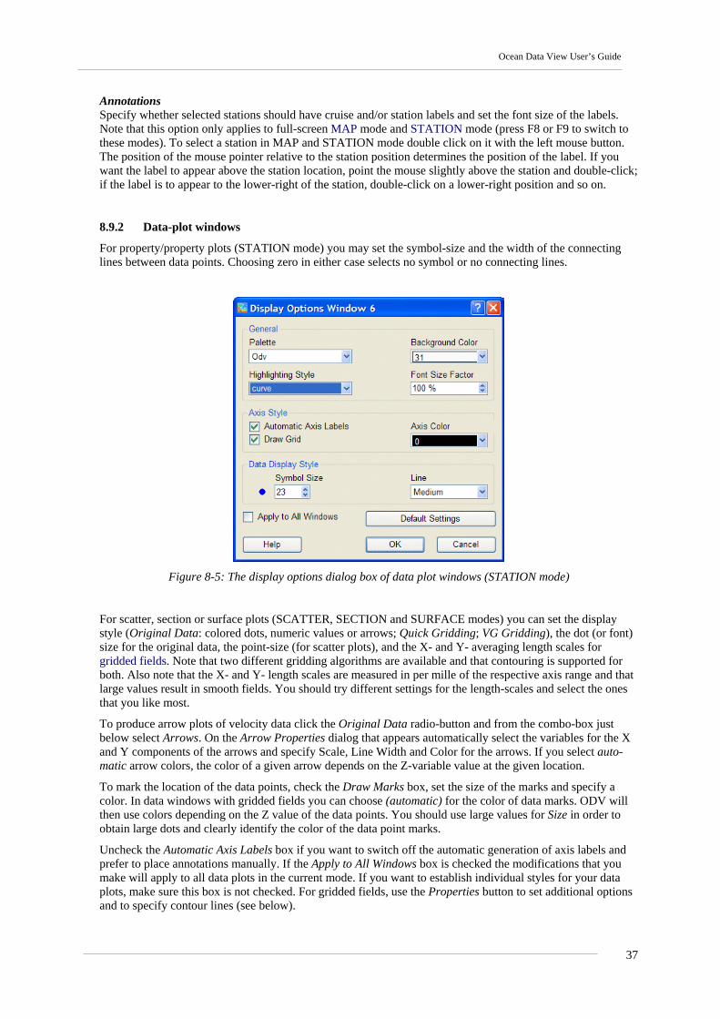
Ocean Data View User’s Guide
Annotations Specify whether selected stations should have cruise and/or station labels and set the font size of the labels. Note that this option only applies to full-screen MAP mode and STATION mode (press F8 or F9 to switch to these modes). To select a station in MAP and STATION mode double click on it with the left mouse button. The position of the mouse pointer relative to the station position determines the position of the label. If you want the label to appear above the station location, point the mouse slightly above the station and double-click; if the label is to appear to the lower-right of the station, double-click on a lower-right position and so on.
8.9.2 Data-plot windows
For property/property plots (STATION mode) you may set the symbol-size and the width of the connecting lines between data points. Choosing zero in either case selects no symbol or no connecting lines.
Figure 8-5: The display options dialog box of data plot windows (STATION mode)
For scatter, section or surface plots (SCATTER, SECTION and SURFACE modes) you can set the display style (Original Data: colored dots, numeric values or arrows; Quick Gridding; VG Gridding), the dot (or font) size for the original data, the point-size (for scatter plots), and the X- and Y- averaging length scales for gridded fields. Note that two different gridding algorithms are available and that contouring is supported for both. Also note that the X- and Y- length scales are measured in per mille of the respective axis range and that large values result in smooth fields. You should try different settings for the length-scales and select the ones that you like most.
To produce arrow plots of velocity data click the Original Data radio-button and from the combo-box just below select Arrows. On the Arrow Properties dialog that appears automatically select the variables for the X and Y components of the arrows and specify Scale, Line Width and Color for the arrows. If you select auto-matic arrow colors, the color of a given arrow depends on the Z-variable value at the given location.
To mark the location of the data points, check the Draw Marks box, set the size of the marks and specify a color. In data windows with gridded fields you can choose (automatic) for the color of data marks. ODV will then use colors depending on the Z value of the data points. You should use large values for Size in order to obtain large dots and clearly identify the color of the data point marks.
Uncheck the Automatic Axis Labels box if you want to switch off the automatic generation of axis labels and prefer to place annotations manually. If the Apply to All Windows box is checked the modifications that you make will apply to all data plots in the current mode. If you want to establish individual styles for your data plots, make sure this box is not checked. For gridded fields, use the Properties button to set additional options and to specify contour lines (see below).
37
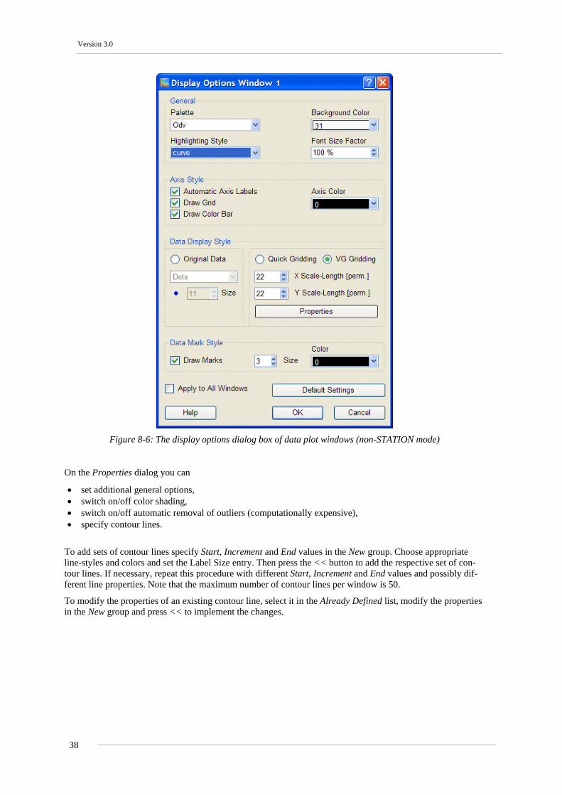
Version 3.0
Figure 8-6: The display options dialog box of data plot windows (non-STATION mode)
On the Properties dialog you can
• set additional general options, • switch on/off color shading, • switch on/off automatic removal of outliers (computationally expensive), • specify contour lines.
To add sets of contour lines specify Start, Increment and End values in the New group. Choose appropriate line-styles and colors and set the Label Size entry. Then press the << button to add the respective set of con-tour lines. If necessary, repeat this procedure with different Start, Increment and End values and possibly dif-ferent line properties. Note that the maximum number of contour lines per window is 50.
To modify the properties of an existing contour line, select it in the Already Defined list, modify the properties in the New group and press << to implement the changes.
38

Ocean Data View User’s Guide
Figure 8-7: The display options properties dialog box
8.10 Printing Choose Print Canvas from the File or canvas popup menus to print the contents of the current ODV graphics window.
WIN32 ODV invokes a standard Windows print-dialog box and lets you select one of the printers available on your system. Press OK to start the printing. Note that print jobs for complicated screen graphics tend to be large and time-consuming. If you have access to a PostScript printer, use the PostScript option instead.
UNIX Not tested.
8.11 PostScript Files To produce PostScript versions of the entire screen or of individual plots, right-click on the canvas or the re-spective data plot and choose Save Canvas As or Save Plot As (alternatively, you can also press Ctrl-S while over the canvas or data plot) and choose PostScript (*.eps) as file type. ODV then presents the PostScript Set-tings dialog and lets you specify the orientation of the PostScript output, set scaling parameters and choose the name and destination of the output file. The resulting PostScript file can be printed by sending it to a Post-Script printer, or it can be imported into LaTex, Word, PageMaker or pdf documents. If you intend to include the eps output file in other documents, make sure to uncheck the Show Collection Info box.
8.12 GIF, PNG and JPG Files You can export the current ODV graphics screen or individual data plots in GIF, PNG or JPG files by choos-ing Save Canvas As from the canvas popup menu or Save Plot As from a data plot popup menu and selecting the respective file type. These options can also be invoked by shortcut key-strokes: (1) pressing Ctrl-S while the mouse is over the canvas area saves the ODV graphics canvas while (2) pressing Ctrl-S with the mouse over the map or a data plot will save the respective data plot. ODV will present a file-save dialog box that lets you choose the appropriate output file type (GIF (*.gif), PNG (*.png) or JPG (*.jpg)). Note that the default output file name is derived from the current configuration name. You can choose any other name or destina-tion, if required. ODV then lets you define the pixel resolution of the output file. The default is to use the graphics resolution of your screen. You can request higher (e.g., 300 dpi) or smaller resolutions, by uncheck-ing the Use Screen Resolution box and specifying the desired resolution. Note that the maximum achievable resolution is limited by the available memory on your system.
39
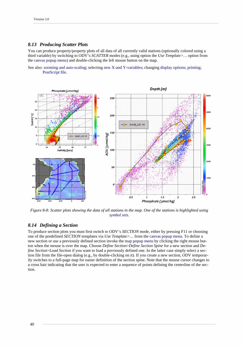
Version 3.0
8.13 Producing Scatter Plots You can produce property/property plots of all data of all currently valid stations (optionally colored using a third variable) by switching to ODV’s SCATTER modes (e.g., using option the Use Template>… option from the canvas popup menu) and double-clicking the left mouse button on the map.
See also: zooming and auto-scaling; selecting new X-and Y-variables; changing display options; printing; PostScript file.
Figure 8-8: Scatter plots showing the data of all stations in the map. One of the stations is highlighted using
symbol sets.
8.14 Defining a Section To produce section plots you must first switch to ODV’s SECTION mode, either by pressing F11 or choosing one of the predefined SECTION templates via Use Template>… from the canvas popup menu. To define a new section or use a previously defined section invoke the map popup menu by clicking the right mouse but-ton when the mouse is over the map. Choose Define Section>Define Section Spine for a new section and De-fine Section>Load Section if you want to load a previously defined one. In the latter case simply select a sec-tion file from the file-open dialog (e.g., by double-clicking on it). If you create a new section, ODV temporar-ily switches to a full-page map for easier definition of the section spine. Note that the mouse cursor changes to a cross hair indicating that the user is expected to enter a sequence of points defining the centerline of the sec-tion.
40

Ocean Data View User’s Guide
Figure 8-9: The GEOSECS western Atlantic section
You enter a point by moving the cross hair to the desired location and clicking the left mouse button. To re-move a point, move the mouse close to it and click the right mouse button. To accept the set of points press ENTER or specify the last point with a double-click of the left mouse button. Note that you may construct rather complicated sections following arbitrary cruise tracks as shown in the picture on the left.
After specifying the section spine, ODV assigns a default width for the section band and selects distance from the starting point (the first point entered) as the default along-section coordinate. A dialog box appears that lets you change the default characteristics of the section. You can change the characteristics of the section at any time by choosing Define Section>Change Characteristics from the map popup menu. Choose among Distance, Longitude and Latitude as along-section coordinate, set the width of the section band, choose a color for the section bathymetry and specify a title for the section. For the section bathymetry you may use station bottom depths or depths from the ETOPO2 global bathymetric dataset. You may also choose to draw no section bathymetry at all. The ETOPO2 item is available in the Bathymetry combo-box after installing the ETOPO2 optional package.
You can save the current section in a file by choosing the Define Section>Save Section As option. You can use saved sections later, by choosing Define Section>Load Section. To undefine a section, select Define Sec-tion>Undefine Section.
Note that all stations inside the section band marked in the map belong to the section and are plotted in subse-quent plot operations.
8.15 Plotting a Section Once you have defined a section you can plot color property distributions along the section and prop-erty/property plots for all stations belonging to the section by double-clicking the left mouse button while over the map or by pressing p. For color property distributions along the section choose Section Coordinate on the X-axis and arbitrary variables for Y and Z.
See also: zooming and auto-scaling; color-zooming; changing the color mapping function; selecting new X, Y-and Z-variables; changing display options; displaying gridded fields; values; printing; PostScript file.
41

Version 3.0
Figure 8-10: The WOCE A16 section
8.16 Color-Zooming Color section plots and color distributions on iso-surfaces allow modifications of the Z-variable ranges by color zooming. To invoke color-zooming move the mouse over the section or iso-surface plot that you want to modify and click the right mouse button to bring up the data plot popup menu. Selecting Z-Zoom will draw a red zoom-frame around the color bar of the respective window. Manipulate and drag this zoom-frame as de-scribed above. To accept the current setting of the zoom-frame and adjust the Z-variable range accordingly double-click the left mouse button or press ENTER. If you want to abort the zoom operation and keep the present variable range, press ESC or click the right mouse button.
8.17 Color Mapping Function For any plot with a Z-variable, such as color section plots or color distributions on iso-surfaces, you can ma-nipulate the color mapping of the Z-variable values. To invoke the color-mapping option move the mouse over the respective plot window and click the right mouse button to bring up the data plot popup menu. Select the Color Mapping option and change the color mapping interactively. For non-linear color-mappings move the Median trackbar to the Z-value which is to receive the highest color-resolution and increase the non-linearity using the Nonlinearity trackbar. Press the Auto Adjust button to establish a possibly non-linear setting based on the Z-variable histogram, or press the Linear Mapping button to restore a linear color mapping. Note that in addition to changing the color mapping function, you can also load different color palettes.
42
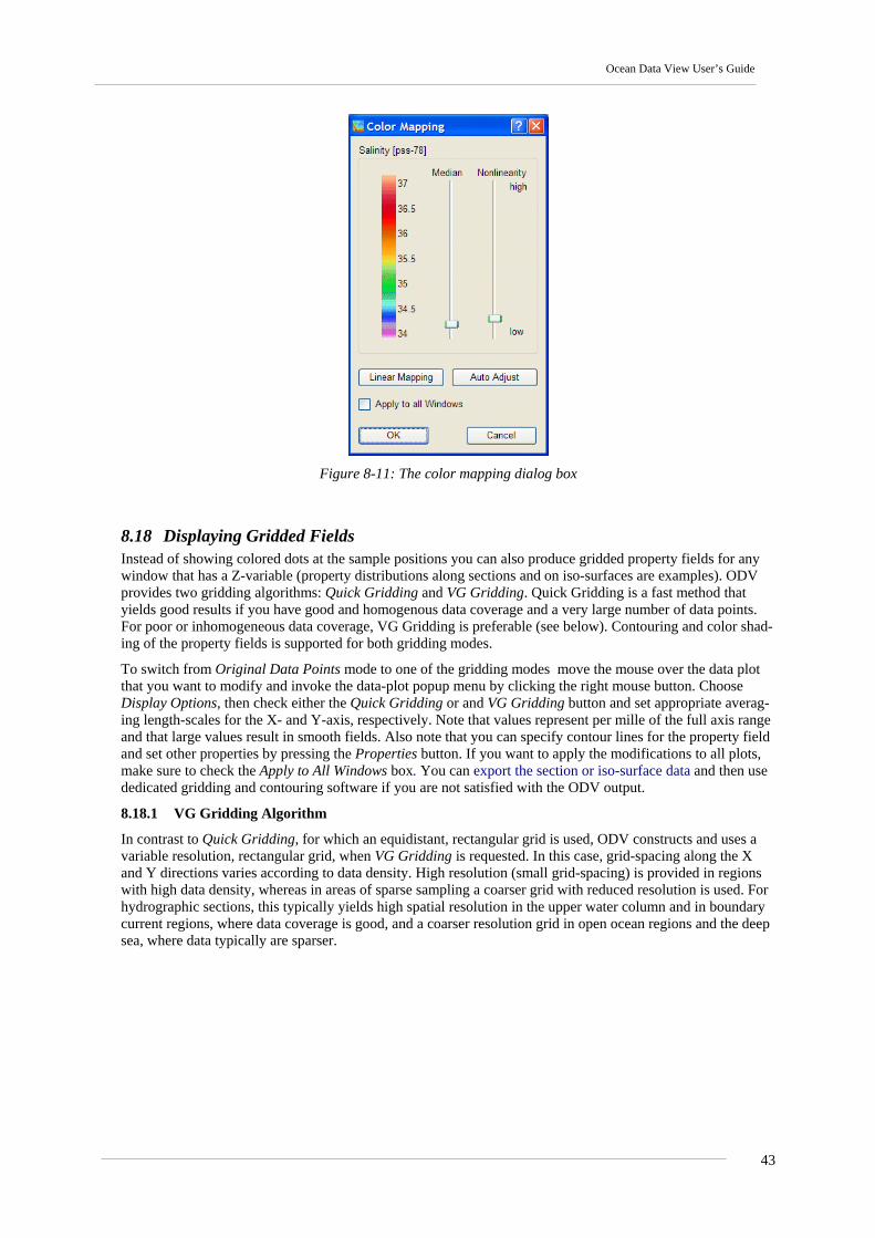
Ocean Data View User’s Guide
Figure 8-11: The color mapping dialog box
8.18 Displaying Gridded Fields Instead of showing colored dots at the sample positions you can also produce gridded property fields for any window that has a Z-variable (property distributions along sections and on iso-surfaces are examples). ODV provides two gridding algorithms: Quick Gridding and VG Gridding. Quick Gridding is a fast method that yields good results if you have good and homogenous data coverage and a very large number of data points. For poor or inhomogeneous data coverage, VG Gridding is preferable (see below). Contouring and color shad-ing of the property fields is supported for both gridding modes.
To switch from Original Data Points mode to one of the gridding modes move the mouse over the data plot that you want to modify and invoke the data-plot popup menu by clicking the right mouse button. Choose Display Options, then check either the Quick Gridding or and VG Gridding button and set appropriate averag-ing length-scales for the X- and Y-axis, respectively. Note that values represent per mille of the full axis range and that large values result in smooth fields. Also note that you can specify contour lines for the property field and set other properties by pressing the Properties button. If you want to apply the modifications to all plots, make sure to check the Apply to All Windows box. You can export the section or iso-surface data and then use dedicated gridding and contouring software if you are not satisfied with the ODV output.
8.18.1 VG Gridding Algorithm
In contrast to Quick Gridding, for which an equidistant, rectangular grid is used, ODV constructs and uses a variable resolution, rectangular grid, when VG Gridding is requested. In this case, grid-spacing along the X and Y directions varies according to data density. High resolution (small grid-spacing) is provided in regions with high data density, whereas in areas of sparse sampling a coarser grid with reduced resolution is used. For hydrographic sections, this typically yields high spatial resolution in the upper water column and in boundary current regions, where data coverage is good, and a coarser resolution grid in open ocean regions and the deep sea, where data typically are sparser.
43

Version 3.0
Figure 8-12: Weighted averaging of data values (red symbols) at a grid node (+). See text for details.
After construction of the grid, property values ∑⋅∑=i
iii
ie dc αα are calculated at every grid point using a
simple weighted-averaging scheme. For efficiency reasons, only data values di from a small neighborhood of the grid-point are considered for summation (see figure above). The weights αi decrease exponentially with increasing distance between data and grid-point: , with and separate averag-ing length-scales L
ri e−=α 22 )/()/( yx LyLxr ∆+∆=
x and Lx in X and Y directions, respectively. Averaging length-scales vary over the domain, and are proportional to local grid-spacing. Thus, small averaging length-scales are used in areas with small grid-spacing (high grid resolution, e.g., in the upper water column or in boundary current regions, etc.), whereas in regions with large grid-spacing, large averaging length-scales are applied automatically. This ap-proach of spatially varying length-scales allows resolving small-scale features in areas of dense data coverage and at the same time provides smooth and stable fields in other regions with sparse data coverage. The user-provided length-scales Lx0 and Ly0 on the Display Options dialog are measured in per-mille of the respective axis range and are representative for the area of poorest data coverage (coarsest grid). The ODV implementa-tion of the weighted averaging algorithm is highly optimized for speed to allow field estimations within a few seconds, even for fields with thousands of data points.
Once estimates have been obtained for all grid nodes, the field is passed to shading and contouring routines for display on the screen or a printer.
8.19 Difference Fields You can compare property distributions of the currently selected stations with previously saved reference data and produce difference fields by defining property differences as derived variables. Choose Derived Variables from ODV’s canvas menu (or press Alt+D) and select Difference from Reference. Then choose the Expor-tID.txt file of the reference dataset that you want to use in one of the subdirectories of reference data directory tree. ODV will show a list of available reference data files from that directory. Select an .oal file that has the variable for which you want to produce the difference field as Z variable and appropriate X and Y variables (e.g., for producing longitude vs. depth sections, make sure the reference data file has longitude as X and depth as Y variable). Then identify the Z, X and Y variables in the current collection (if longitude or latitude are required, define them as derived variables prior to invoking the Difference from Reference option) to complete the definition of the difference variable. Note that the name of the new variable is composed of the name of the Z variable and the identification string of the reference data set. Once defined, you can use the difference variable in any data plot.
8.20 Defining Iso-Surfaces After switching to SURFACE mode (by pressing F12 or selecting one of the predefined SURFACE templates), ODV enables the Iso-Surface Variables option on the canvas popup menu and allows the definition of iso-surface variables. ODV shows a list of currently defined iso-surface variables and lets you edit and delete existing iso-surface variables or create new ones. To delete an existing iso-surface variable double-click on it with the left mouse or select it using a single left mouse click and press Delete. To add a new iso-surface vari-able first construct it inside the New box and then press Add. Constructing an iso-surface variable requires that you specify the variable that you want to display on a given surface (display variable), the variable that defines the surface (surface variable) and a numeric value for the surface variable. For top or bottom property distribu-
44
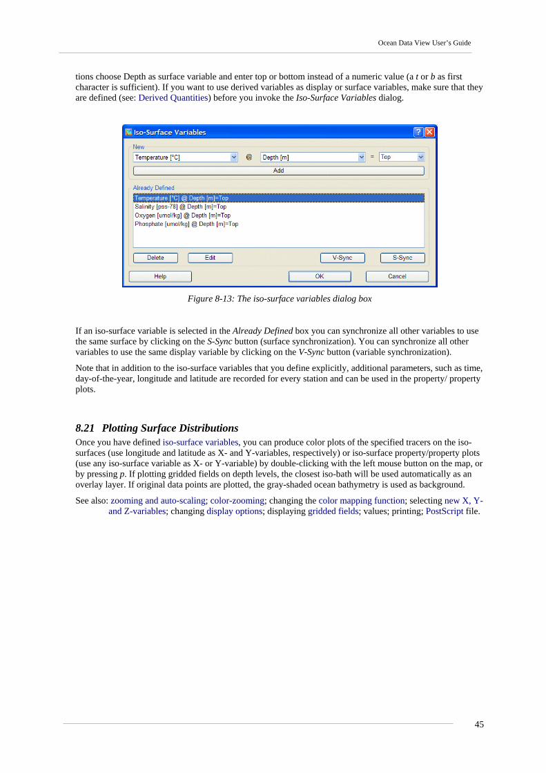
Ocean Data View User’s Guide
tions choose Depth as surface variable and enter top or bottom instead of a numeric value (a t or b as first character is sufficient). If you want to use derived variables as display or surface variables, make sure that they are defined (see: Derived Quantities) before you invoke the Iso-Surface Variables dialog.
Figure 8-13: The iso-surface variables dialog box
If an iso-surface variable is selected in the Already Defined box you can synchronize all other variables to use the same surface by clicking on the S-Sync button (surface synchronization). You can synchronize all other variables to use the same display variable by clicking on the V-Sync button (variable synchronization).
Note that in addition to the iso-surface variables that you define explicitly, additional parameters, such as time, day-of-the-year, longitude and latitude are recorded for every station and can be used in the property/ property plots.
8.21 Plotting Surface Distributions Once you have defined iso-surface variables, you can produce color plots of the specified tracers on the iso-surfaces (use longitude and latitude as X- and Y-variables, respectively) or iso-surface property/property plots (use any iso-surface variable as X- or Y-variable) by double-clicking with the left mouse button on the map, or by pressing p. If plotting gridded fields on depth levels, the closest iso-bath will be used automatically as an overlay layer. If original data points are plotted, the gray-shaded ocean bathymetry is used as background.
See also: zooming and auto-scaling; color-zooming; changing the color mapping function; selecting new X, Y-and Z-variables; changing display options; displaying gridded fields; values; printing; PostScript file.
45

Version 3.0
Figure 8-14: Temperature and salinity distributions on iso-surfaces
46
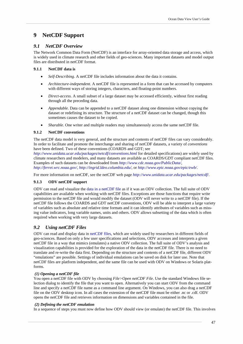
Ocean Data View User’s Guide
9 NetCDF Support
9.1 NetCDF Overview The Network Common Data Form (NetCDF) is an interface for array-oriented data storage and access, which is widely used in climate research and other fields of geo-sciences. Many important datasets and model output files are distributed in netCDF format.
9.1.1 NetCDF data is
• Self-Describing. A netCDF file includes information about the data it contains.
• Architecture-independent. A netCDF file is represented in a form that can be accessed by computers with different ways of storing integers, characters, and floating-point numbers.
• Direct-access. A small subset of a large dataset may be accessed efficiently, without first reading through all the preceding data.
• Appendable. Data can be appended to a netCDF dataset along one dimension without copying the dataset or redefining its structure. The structure of a netCDF dataset can be changed, though this sometimes causes the dataset to be copied.
• Sharable. One writer and multiple readers may simultaneously access the same netCDF file.
9.1.2 NetCDF conventions
The netCDF data model is very general, and the structure and contents of netCDF files can vary considerably. In order to facilitate and promote the interchange and sharing of netCDF datasets, a variety of conventions have been defined. Two of these conventions (COARDS and GDT; see http://www.unidata.ucar.edu/packages/netcdf/conventions.html for detailed specifications) are widely used by climate researchers and modelers, and many datasets are available as COARDS/GDT compliant netCDF files. Examples of such datasets can be downloaded from http://www.cdc.noaa.gov/PublicData/, http://ferret.wrc.noaa.gov/, http://ingrid.ldeo.columbia.edu/, or http://www.epic.noaa.gov/epic/ewb/.
For more information on netCDF, see the netCDF web page http://www.unidata.ucar.edu/packages/netcdf/.
9.1.3 ODV netCDF support
ODV can read and visualize the data in a netCDF file as if it was an ODV collection. The full suite of ODV capabilities are available when working with netCDF files. Exceptions are those functions that require write permission to the netCDF file and would modify the dataset (ODV will never write to a netCDF file). If the netCDF file follows the COARDS and GDT netCDF conventions, ODV will be able to interpret a large variety of variables such as absolute and relative time formats and it can identify attributes of variables such as miss-ing value indicators, long variable names, units and others. ODV allows subsetting of the data which is often required when working with very large datasets.
9.2 Using netCDF Files ODV can read and display data in netCDF files, which are widely used by researchers in different fields of geo-sciences. Based on only a few user specifications and selections, ODV accesses and interprets a given netCDF file in a way that mimics (emulates) a native ODV collection. The full suite of ODV’s analysis and visualization capabilities is provided for the exploration of the data in the netCDF file. There is no need to translate and re-write the data first. Depending on the structure and contents of a netCDF file, different ODV “emulations” are possible. Settings of individual emulations can be saved on disk for later use. Note that netCDF files are platform independent, and the same file can be used with ODV on Windows or Solaris plat-forms.
(1) Opening a netCDF file You open a netCDF file with ODV by choosing File>Open netCDF File. Use the standard Windows file se-lection dialog to identify the file that you want to open. Alternatively you can start ODV from the command line and specify a netCDF file name as a command line argument. On Windows, you can also drag a netCDF file on the ODV desktop icon. In all cases the extension of the netCDF file must be either .nc or .cdf. ODV opens the netCDF file and retrieves information on dimensions and variables contained in the file.
(2) Defining the netCDF emulation In a sequence of steps you must now define how ODV should view (or emulate) the netCDF file. This involves
47

Version 3.0
selection and subsetting (if required) of coordinate axis (dimensions), association of ODV header variables with information from the netCDF file and the definition of the primary variable (first variable in an ODV collection), which determines the logical structure of a “station” (e.g., profile, sequence, etc.) and the sort-order within a station.
ODV first asks whether a new emulation is to be defined or whether a previously defined and saved emulation should be used. If you choose a previously defined emulation, no additional input is required and ODV pro-ceeds as if it was using a native ODV collection: it draws a station map and offers the full suite of ODV analy-sis and display capabilities. Note that ODV will not modify an open netCDF file and treats it as a read-only dataset. As a consequence, all ODV functions that require data-write operations (data import, header and data editing, collection manipulation operations, etc.) are disabled when working with netCDF files.
(2.a) Selecting netCDF coordinates If you define a new emulation, the first step is to select netCDF coordinates. ODV will show a list of coordi-nates contained in the file.
Figure 9-1: The netCDF emulation dialog (step 1 of 4)
Using extended selection techniques (hold down the Ctrl or Shft keys while clicking the left mouse button) select all the coordinates that you want to use. If multiple coordinates are provided for the common coordi-nates X (Longitude), Y (Latitude), Z (Depth/Height), and T (Time), make sure to select only one for each direction.
For a given selection of coordinates, the set of netCDF variables that are defined on these dimensions is shown in the Corresponding Variables list. Make sure that the variables that you are interested in are shown in this list. Other variables in the netCDF file that depend on coordinates not selected in the Dimensions list are not shown as Corresponding Variables. These variables will remain unavailable unless you select the correspond-ing dimensions. To view the complete header information of the netCDF file (similar to a “ncdump –h” call) press netCDF Info.
(2.b) Specifying header information Next, you must identify the netCDF variables that provide header (or meta-) information for the ODV stations: e.g., longitude (Longitude [degrees_east]), latitude (Latitude [degrees_north]), date (mon/day/yr), etc. This is done by establishing associations between variables from the netCDF file (Source Variables list) and the ODV header variables (Target Variables list). ODV will try to identify and associate variables automatically. Man-ual association of variables is only necessary for those header variables not marked by a * in the first column. Usually it is sufficient to associate Longitude [degrees_east], Latitude [degrees_north], and mon/day/yr. For header variables not associated with any netCDF variable, ODV uses default settings. You can modify the default value for a header variable (e.g., Cruise, etc.) by selecting it in the Target Variables list and pressing Set Default.
To establish a (1-to-1) association between a netCDF variable and an ODV header variable, select the netCDF variable in the Source Variables list and the header variable in the Target Variables list and press Associate. To establish a conversion between a netCDF and ODV header variable (usually needed for netCDF time vari-ables), select the two variables as above and then press Convert. Choose one of the available conversion op-tions from the combo-box and press OK. For the General Linear Transformation provide a scale factor and an
48
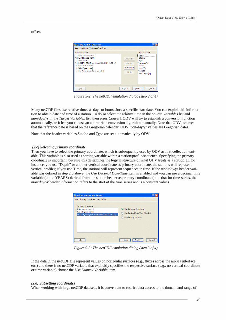
Ocean Data View User’s Guide
offset.
Figure 9-2: The netCDF emulation dialog (step 2 of 4)
Many netCDF files use relative times as days or hours since a specific start date. You can exploit this informa-tion to obtain date and time of a station. To do so select the relative time in the Source Variables list and mon/day/yr in the Target Variables list, then press Convert. ODV will try to establish a conversion function automatically, or it lets you choose an appropriate conversion algorithm manually. Note that ODV assumes that the reference date is based on the Gregorian calendar. ODV mon/day/yr values are Gregorian dates.
Note that the header variables Station and Type are set automatically by ODV.
(2.c) Selecting primary coordinate Then you have to select the primary coordinate, which is subsequently used by ODV as first collection vari-able. This variable is also used as sorting variable within a station/profile/sequence. Specifying the primary coordinate is important, because this determines the logical structure of what ODV treats as a station. If, for instance, you use “Depth” or another vertical coordinate as primary coordinate, the stations will represent vertical profiles; if you use Time, the stations will represent sequences in time. If the mon/day/yr header vari-able was defined in step 2.b above, the Use Decimal Date/Time item is enabled and you can use a decimal time variable (units=YEARS) derived from the station header as primary coordinate (note that for time-series, the mon/day/yr header information refers to the start of the time series and is a constant value).
Figure 9-3: The netCDF emulation dialog (step 3 of 4)
If the data in the netCDF file represent values on horizontal surfaces (e.g., fluxes across the air-sea interface, etc.) and there is no netCDF variable that explicitly specifies the respective surface (e.g., no vertical coordinate or time variable) choose the Use Dummy Variable item.
(2.d) Subsetting coordinates When working with large netCDF datasets, it is convenient to restrict data access to the domain and range of
49
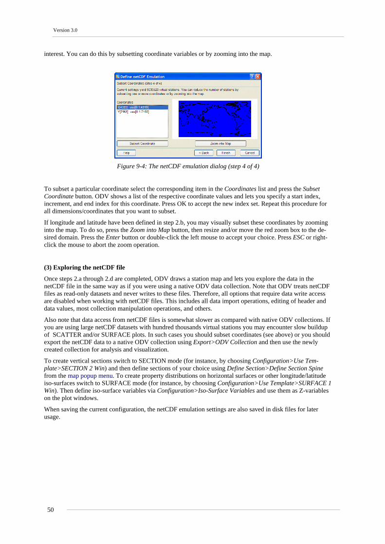
Version 3.0
interest. You can do this by subsetting coordinate variables or by zooming into the map.
Figure 9-4: The netCDF emulation dialog (step 4 of 4)
To subset a particular coordinate select the corresponding item in the Coordinates list and press the Subset Coordinate button. ODV shows a list of the respective coordinate values and lets you specify a start index, increment, and end index for this coordinate. Press OK to accept the new index set. Repeat this procedure for all dimensions/coordinates that you want to subset.
If longitude and latitude have been defined in step 2.b, you may visually subset these coordinates by zooming into the map. To do so, press the Zoom into Map button, then resize and/or move the red zoom box to the de-sired domain. Press the Enter button or double-click the left mouse to accept your choice. Press ESC or right-click the mouse to abort the zoom operation.
(3) Exploring the netCDF file
Once steps 2.a through 2.d are completed, ODV draws a station map and lets you explore the data in the netCDF file in the same way as if you were using a native ODV data collection. Note that ODV treats netCDF files as read-only datasets and never writes to these files. Therefore, all options that require data write access are disabled when working with netCDF files. This includes all data import operations, editing of header and data values, most collection manipulation operations, and others.
Also note that data access from netCDF files is somewhat slower as compared with native ODV collections. If you are using large netCDF datasets with hundred thousands virtual stations you may encounter slow buildup of SCATTER and/or SURFACE plots. In such cases you should subset coordinates (see above) or you should export the netCDF data to a native ODV collection using Export>ODV Collection and then use the newly created collection for analysis and visualization.
To create vertical sections switch to SECTION mode (for instance, by choosing Configuration>Use Tem-plate>SECTION 2 Win) and then define sections of your choice using Define Section>Define Section Spine from the map popup menu. To create property distributions on horizontal surfaces or other longitude/latitude iso-surfaces switch to SURFACE mode (for instance, by choosing Configuration>Use Template>SURFACE 1 Win). Then define iso-surface variables via Configuration>Iso-Surface Variables and use them as Z-variables on the plot windows.
When saving the current configuration, the netCDF emulation settings are also saved in disk files for later usage.
50
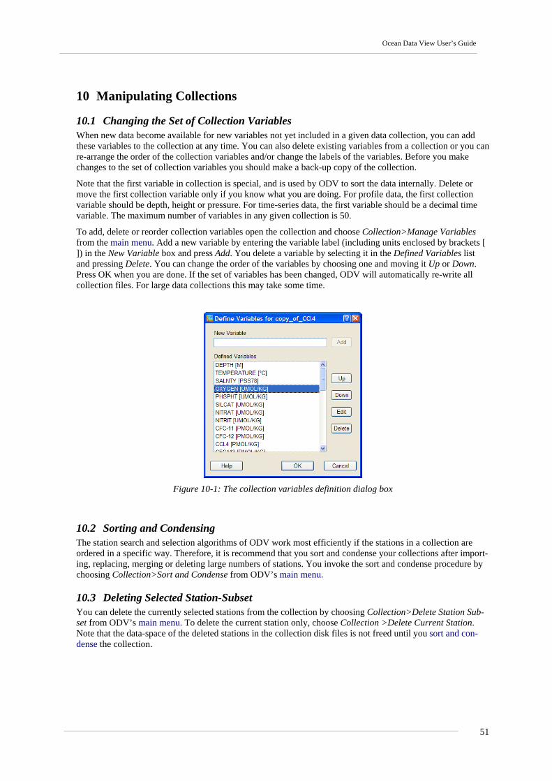
Ocean Data View User’s Guide
10 Manipulating Collections
10.1 Changing the Set of Collection Variables When new data become available for new variables not yet included in a given data collection, you can add these variables to the collection at any time. You can also delete existing variables from a collection or you can re-arrange the order of the collection variables and/or change the labels of the variables. Before you make changes to the set of collection variables you should make a back-up copy of the collection.
Note that the first variable in collection is special, and is used by ODV to sort the data internally. Delete or move the first collection variable only if you know what you are doing. For profile data, the first collection variable should be depth, height or pressure. For time-series data, the first variable should be a decimal time variable. The maximum number of variables in any given collection is 50.
To add, delete or reorder collection variables open the collection and choose Collection>Manage Variables from the main menu. Add a new variable by entering the variable label (including units enclosed by brackets [ ]) in the New Variable box and press Add. You delete a variable by selecting it in the Defined Variables list and pressing Delete. You can change the order of the variables by choosing one and moving it Up or Down. Press OK when you are done. If the set of variables has been changed, ODV will automatically re-write all collection files. For large data collections this may take some time.
Figure 10-1: The collection variables definition dialog box
10.2 Sorting and Condensing The station search and selection algorithms of ODV work most efficiently if the stations in a collection are ordered in a specific way. Therefore, it is recommend that you sort and condense your collections after import-ing, replacing, merging or deleting large numbers of stations. You invoke the sort and condense procedure by choosing Collection>Sort and Condense from ODV’s main menu.
10.3 Deleting Selected Station-Subset You can delete the currently selected stations from the collection by choosing Collection>Delete Station Sub-set from ODV’s main menu. To delete the current station only, choose Collection >Delete Current Station. Note that the data-space of the deleted stations in the collection disk files is not freed until you sort and con-dense the collection.
51
Version 3.0
11 Utilities
11.1 Data Inventory Tables You can produce an inventory table of the currently open collection by choosing Utilities>Inventory Table from ODV’s main menu. The output file is plain ASCII and is written to the collection directory (extension .inv).
11.2 Geostrophic Flows In SECTION mode, ODV lets you calculate and visualize geostrophic velocities via the Utilities>Geostrophic Flows option. Define a reference layer by choosing a depth horizon or a specific value for any other basic or derived variable (i.e., potential density, etc.) and specify the name of the .o4x output file that receives the re-sults. Note that by default this file is written to subdirectory GeoVel of the collection directory (this subdirec-tory is created automatically if not already present). ODV will start the calculations and export the station-pair results and geostrophic velocities to the .o4x file specified above.
Once completed, ODV allows you to invoke a new ODV session on the newly calculated section pair and velocity data. If you click on Yes, the new ODV will create a new collection in the GeoVel directory and will automatically import the .o4x file just written. Using standard ODV procedures, you should then define an appropriate map domain by zooming into the map, you should switch to SECTION mode by pressing F11, and you should define Geostr. Vel. [cm/s], Geostr. Vel. (north comp.) [cm/s] and/or Geostr. Vel. (east comp.) [cm/s] as Z-variable of one or more plot windows. The station label of a given station-pair A->B:alpha consists of the original station numbers A and B of the stations used in the pair and the direction alpha of flow for posi-tive values of Geostr. Vel. [cm/s] (alpha=0: eastward; alpha=90: northward; etc.).
Geostrophic velocities are derived from dynamic height differences between two hydrographic stations. Be-cause, in general, the observed depths for the two stations do not match, in a first step the measurements have to be mapped to a set of common depths (ODV uses piecewise linear least squares for the interpolation on a predefined set of standard depths). Then dynamic heights at the standard depths are calculated for both sta-tions, and the geostrophic velocities for the station pair (at the standard depths) are obtained from the dynamic height differences. ODV also calculates average values for all variables in the collection (pair-averages). Both, the pair-averages and the geostrophic velocities are representative for the mid-point between the two stations involved, and ODV writes those values to the output .o4x file for a “virtual” pair station located at the mid-point between the two stations in the pair (note the station label of the pair station contains the station labels of the original stations involved).
Note that geostrophic velocities are not calculated close to the Equator or for stations with sparse hydrographic observations. Because results are very sensitive to data errors, you should quality control the temperature and salinity data of the section carefully prior to invoking the Utilities>Geostrophic Flows option. One way to proceed is to flag suspicious data as Questionable or Bad using the Edit Data option and to accept only Good and Unknown data by applying appropriate selection criteria. Also, by applying appropriate station selection criteria, you should make sure that only stations for a given expedition are included in the calculations and that stations from other cruises are excluded (watch out for other oceanographic lines crossing the section-band).
11.3 3D Estimation You can estimate values for a basic or derived variable at arbitrary geographical locations by choosing Utili-ties>3D Estimation. ODV will prompt you for a ASCII file that contains the longitude, latitude, and depth values of the points for which Z-variable estimates are to be obtained. This 3D point definition file has to be prepared prior to invoking the Utilities>3D Estimation option. When creating the point definition file, specify one point per line, and provide decimal longitude, latitude and depth values in this order, with one or more spaces separating the individual values. ODV will let you choose the variable for which the estimation should be performed and it lets you specify x/y/z averaging length scales used for the estimation. Note that the length scale units for longitude and latitude are in per mille of the current map ranges, whereas the unit of the depth length scale is in meters. Choosing large values for the averaging length scales will result in smooth estimates. For the 3D Estimation all original data points from all stations currently shown in the map will be used. The weight with which a given data point influences the estimate at a specific target location is inversely propor-tional to the distance between data and target points.
52
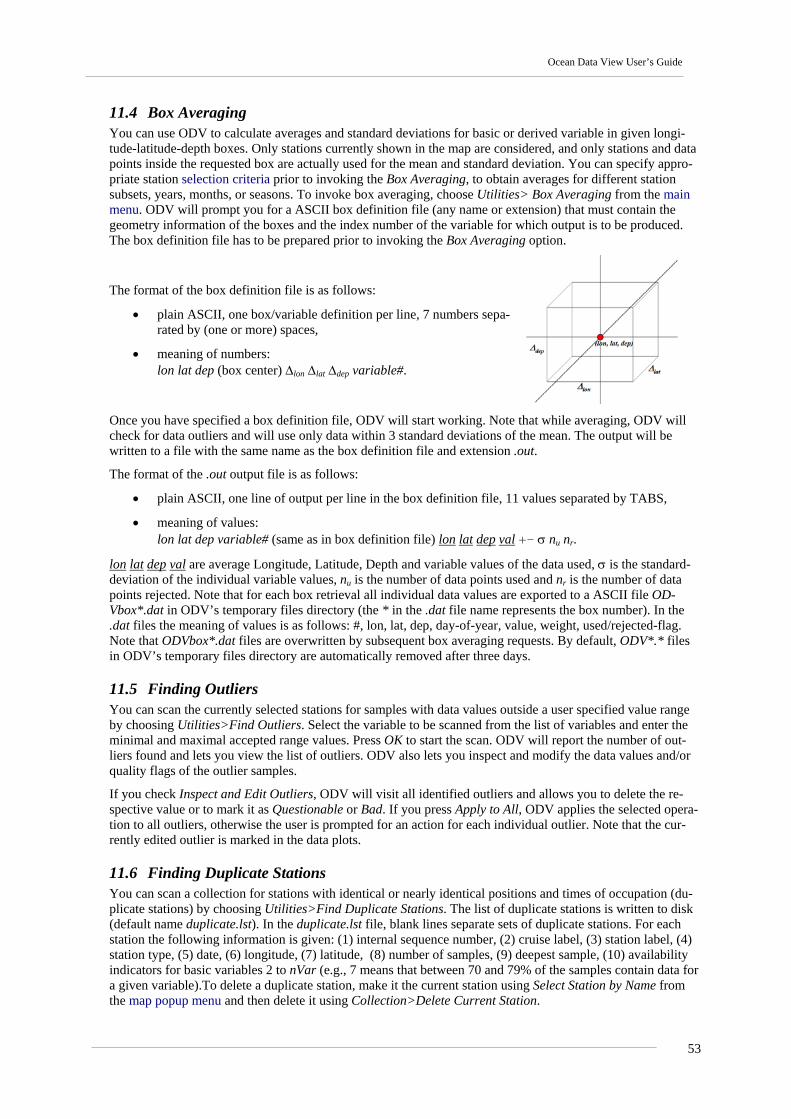
Ocean Data View User’s Guide
11.4 Box Averaging You can use ODV to calculate averages and standard deviations for basic or derived variable in given longi-tude-latitude-depth boxes. Only stations currently shown in the map are considered, and only stations and data points inside the requested box are actually used for the mean and standard deviation. You can specify appro-priate station selection criteria prior to invoking the Box Averaging, to obtain averages for different station subsets, years, months, or seasons. To invoke box averaging, choose Utilities> Box Averaging from the main menu. ODV will prompt you for a ASCII box definition file (any name or extension) that must contain the geometry information of the boxes and the index number of the variable for which output is to be produced. The box definition file has to be prepared prior to invoking the Box Averaging option.
The format of the box definition file is as follows:
• plain ASCII, one box/variable definition per line, 7 numbers sepa-rated by (one or more) spaces,
• meaning of numbers: lon lat dep (box center) ∆lon ∆lat ∆dep variable#.
Once you have specified a box definition file, ODV will start working. Note that while averaging, ODV will check for data outliers and will use only data within 3 standard deviations of the mean. The output will be written to a file with the same name as the box definition file and extension .out.
The format of the .out output file is as follows:
• plain ASCII, one line of output per line in the box definition file, 11 values separated by TABS,
• meaning of values: lon lat dep variable# (same as in box definition file) lon lat dep val +- σ nu nr.
lon lat dep val are average Longitude, Latitude, Depth and variable values of the data used, σ is the standard-deviation of the individual variable values, nu is the number of data points used and nr is the number of data points rejected. Note that for each box retrieval all individual data values are exported to a ASCII file OD-Vbox*.dat in ODV’s temporary files directory (the * in the .dat file name represents the box number). In the .dat files the meaning of values is as follows: #, lon, lat, dep, day-of-year, value, weight, used/rejected-flag. Note that ODVbox*.dat files are overwritten by subsequent box averaging requests. By default, ODV*.* files in ODV’s temporary files directory are automatically removed after three days.
11.5 Finding Outliers You can scan the currently selected stations for samples with data values outside a user specified value range by choosing Utilities>Find Outliers. Select the variable to be scanned from the list of variables and enter the minimal and maximal accepted range values. Press OK to start the scan. ODV will report the number of out-liers found and lets you view the list of outliers. ODV also lets you inspect and modify the data values and/or quality flags of the outlier samples.
If you check Inspect and Edit Outliers, ODV will visit all identified outliers and allows you to delete the re-spective value or to mark it as Questionable or Bad. If you press Apply to All, ODV applies the selected opera-tion to all outliers, otherwise the user is prompted for an action for each individual outlier. Note that the cur-rently edited outlier is marked in the data plots.
11.6 Finding Duplicate Stations You can scan a collection for stations with identical or nearly identical positions and times of occupation (du-plicate stations) by choosing Utilities>Find Duplicate Stations. The list of duplicate stations is written to disk (default name duplicate.lst). In the duplicate.lst file, blank lines separate sets of duplicate stations. For each station the following information is given: (1) internal sequence number, (2) cruise label, (3) station label, (4) station type, (5) date, (6) longitude, (7) latitude, (8) number of samples, (9) deepest sample, (10) availability indicators for basic variables 2 to nVar (e.g., 7 means that between 70 and 79% of the samples contain data for a given variable).To delete a duplicate station, make it the current station using Select Station by Name from the map popup menu and then delete it using Collection>Delete Current Station.
53

Version 3.0
12 Graphics Objects You can add text annotations, symbols, lines and other geometric objects to the ODV graphics canvas, thereby giving it a finishing, professional touch. The following graphics objects are supported: (1) text annotations, (2) straight lines, (3) rectangles and squares, (4) ellipses and circles, (5) polylines (straight-line segments or Bezier smoothed), (6) filled polygons (straight-line segments or Bezier smoothed), (7) symbols, (8) symbol sets and (9) legends. Detailled descriptions of these objects follow below.
Any ODV graphics object is owned by the graphics canvas, the map or a specific data plot window. The ob-jects are drawn, whenever the respective parent object is drawn. The coordinates of a graphics object are either specified in the coordinate system of the owner window or of the graphics canvas (coordinates of the back-ground are in cm from the lower left corner). The initial owner and coordinate system of an object are the window, from which creation was initiated (see below). Like most other properties of a graphics object, own-nership and the coordinate system may be edited and modified at any time.
All graphics objects are part of the current configuration, and they are stored in the cfg file of this configura-tion.
Creation Except for legends, which are created automatically, you create and add any other graphics object by choosing Extras>Add Graphics Object>... (”...” represents the desired object type) from the map or data plot popup menus or by choosing Add Graphics Object>... from the canvas popup menu. After initial creation, dialog boxes appear that let you define various properties of the object. These properties can be changed (see ”Edit” below) at any time. A graphics object is owned by the window (or canvas area) from which the creation was initiated, and the coordinates of the graphics object are in the respective window coordinate system. As a con-sequence, all objects of a window follow automatically when the respective window is moved or resized.
Graphics objects can also be created as copies of existing objects via the Copy Object option of the graphics object context menu, or the Copy button of the graphics objects management dialog (see below). You may also import graphics objects from ODV .gob files, previously created by exporting existing graphics objects or window objects, such as bathymetry polygons from section plots, contour lines from gridded field plots, col-ored data points from any data plot with a Z-variable or the selection polygon from station maps.
Edit and Delete The properties of a given object can be modified by moving the mouse over it (for symbol sets move the mouse over one of the symbols), clicking the right mouse button and choosing Edit Object from the popup menu. Dialog boxes (different for the different objects) appear and let you change properties easily and quickly. Any graphics object may be clipped to its parent window (check the clip to window box), and you may request that it is drawn before the data of the window are drawn (check the pre-data plot box).You delete an object by moving the mouse over it, clicking the right mouse button and choosing Delete Object.
Dragging If the attribute allow dragging of a graphics object is set, the object can be re-positioned by simply dragging it to a different location. To drag an object, move the mouse over it, click and hold down the left mouse button and move the mouse. By default, dragging is switched on initially for all graphics objects except symbol sets linked to actual data values. You can change the allow dragging attribute at any time using the respective Edit dialog (see above).
Managing Graphics Objects You can manage the graphics objects of the canvas, map or any data plot using the respective Extras>Manage Graphics Objects option. You may edit, export, copy, re-order and delete single items or groups of selected objects.
12.1 Annotations You can add annotations to the ODV graphics window by choosing (Extras>)Add Graphics Ob-ject>Annotation from the canvas, map or data plot popup menus. A cross-hair cursor will appear, and you should move it to the location where the annotation should appear and then click the left mouse button. Note that the window from which the creation was initiated owns the respective object. When adding (or editing) annotations you may set the position, orientation (degrees, counter-clockwise), font size (pt), color and align-ment parameter of the annotation text. Annotations can have a frame, and the annotation rectangle can be filled
54

Ocean Data View User’s Guide
before drawing the annotation. You can choose different colors for these items. Note that the maximum length of the annotation text is 255 characters. In ODV annotions, you can use various formatting control sequences as well as functions for auto-text substitution.
Like all graphics objects, you can drag an annotation to a different position by moving the mouse cursor over it, pressing and holding down the left mouse button and moving the mouse. You can edit an annotation by moving the mouse over it, clicking the right mouse button and choosing Edit Object from the popup menu. To delete an annotation (all annotations) choose Delete Object (Delete All Objects) from its popup menu.
Note that the axis labels of the data plot windows are implemented as (automatic) annotations. They are cre-ated automatically when the plot window is drawn and they are deleted when the respective data plot window is deleted. You can drag, edit or delete axis labels, but please note that the automatic versions re-appear if the plot window is redrawn. If you want to change an axis label permanently, you should create an annotation manually by choosing Extras>Add Graphics Object>Annotation from the canvas popup menu. Make sure that you save the configuration after defining the new annotation and delete the automatic axis annotation before printing or writing PostScript files.
12.2 Lines and Polygons You add straight lines, polylines and polygons to the map, data plots or canvas by choosing (Extras>)Add Graphics Object>Line, ...>Polyline or ...>Polygon from the map, data plot or canvas popup menus. In all three cases the cursor changes to a cross hair and you should proceed by specifying the nodes of the object. For a ”Line” you must define starting- and endpoint: move the cross-hair to the start of the line and click the left mouse button, then move to the end-point and click the left button again. For Polyline or Polygon you may define up 1000 points. Note that polygons are closed automatically by ODV. If you want to delete a point, move the cross hair close to it and click the right mouse button. You end the definition of polygon or polyline points by pressing ENTER.
Once you have specified the nodes of the line, polyline or polygon, ODV presents a dialog box that lets you define color, width and type of the (poly)line and the fill-color of the polygon (ignored for Line and Polyline; choose ”none” as fill-color to avoid filling of the polygon). Also note that lines wider than 1 pixel are always solid on many screen and printer devices. However, the requested line-type is always honored in ODV Post-Script files. Polylines and polygons may be smoothed by checking the Bezier smoothing box.
12.3 Rectangles and Ellipses You add rectangles (squares) and ellipses (circles) to the map, data plots or canvas by choosing (Extras>)Add Graphics Object>Rectangle, or ...>Ellipse from the map, data plot or canvas popup menus. A red zoom rec-tangle will appear that represents the bounding box of the new rectangle or ellipse. The zoom rectangle can be moved and resized, press ENTER to accept a setting. A dialog box appears that lets you define properties of the rectangle or ellipse (for details see Lines and Polygons).
12.4 Symbols You add symbols (dots, squares, diamonds, triangles, inverted triangles, stars, crosses, pluses) to the map, data plots or canvas by choosing (Extras>)Add Graphics Object>Symbol from the map, data plot or canvas popup menus. A cross-hair cursor will appear, and you should move it to the location where the symbol should ap-pear. Then click the left mouse button. The Symbol Properties dialog box appears and lets you set various symbol properties.
12.5 Symbol Sets and Legends You can highlight a subset of the data points in a plot window or a subset of stations in the map by assigning a symbol to the selected data points (symbol-set). To create a symbol-set for a data window or the map, move the mouse over this window and choose Extras>Add Graphics Object>Symbol Set. The symbol set selection dialog box appears and lets you select the subset of data points (specify cruise labels, stations and/or individual samples). Press the << button to add the points to the list of selections. Press OK once all desired points are selected. Then the symbol set properties dialog box appears which lets you define the symbol characteristics. A symbol set can have a descriptive text (legend), which will automatically be added to the legends of the respective window (check the add to legends box). Unlike other graphics objects, symbol sets cannot be dragged because they are associated with the selected data points. You can change all properties of a symbol set at any time by moving the mouse over any one of its symbols, clicking the right mouse button and choos-
55

Version 3.0
ing Edit Graphics Object.
If a data window or the map contain symbol sets with the add to legends option switched on, a legend box containing the symbol and legend text of all symbol sets for this window appears. Legend sets can be dragged to different locations and their properties (the size of the legend box is modified by changing the font size for the legend text) can be modified at any time (move mouse over legend set, click right mouse button and choose Edit Graphics Object).
Figure 12-1: Sample scatter plot using symbols sets and legends to highlight the data of a particular station
56
Ocean Data View User’s Guide
13 More …
13.1 Gazetteer of Undersea Features ODV can be used to identify undersea features like seamounts, ridges, fracture zones, troughs, basins, etc. To invoke the gazetteer option, choose Extras>Gazetteer from the map popup menu (or press Ctrl-g while the mouse is over the map). The gazetteer dialog box is shown and lets you select a specific database, lets you specify feature selection criteria as well as size and color of the gazetteer marks drawn by ODV. When you press the Switch On button (or Update, if you have modified the gazetteer settings), the information from the selected gazetteer database is loaded, and the feature positions are marked in the map. Moving the mouse close to a feature point invokes a popup window displaying the name of the feature. To switch off the gazetteer marks, invoke the gazetteer dialog box again and press the Switch Off button.
A number of gazetteer files are provided with the ODV distribution. These include: (1) GazetteerGEBCO.gzt from the International Hydrographic Bureau (IHB), (2) GazetteerBGN.gzt from the US Defense Mapping Agency, and (3) WHP_Sections.gzt, which is a compilation of the sections occupied during the WOCE Hydro-graphic Programme. You can produce feature subsets by specifying a feature type and/or feature name sub-string using the gazetteer dialog box. Note that the name and type selections are case-insensitive. Use the gaz-etteer feature selection if you know the name of a feature (or part of the name) and want to identify its location (note that you might have to open the map to global extent in order to see the feature mark). Gazetteer settings are not saved in configuration files. Whenever you open a collection, the gazetteer option is switched off ini-tially and you have to switch it on in order to use it.
Gazetteer files can be edited and extended. You can also create your own, new gazetteer databases. In order to use a private gazetteer with ODV, the file must have the extension .gzt, it must be located in the ODV gazet-teer directory (normally: c:\Program Files\Ocean Data View (mp)\include\gazetteers) and its format must sat-isfy the specifications below:
The first line of the file must start with % GZT01: followed by the name of the file.
Then there are 7 lines starting with % and containing arbitrary comments.
The next line must be: Feature;Type;No;East-Longitude;North-Latitude; there has to be one blank line following.
The rest of the file contains the actual item definitions. Each feature is listed on a separate line.
The name of the feature, its type, the number of longitude/latitude points and the longitude/latitude entries are separated by semicolons ”;”. Longitude is specified in degrees East (0-360). The number of longi-tude/latitude points can be up to 1500, and the length of a line may be up to 200,000 characters.
13.2 Drag-and-Drop On most platforms you can drag and drop ODV supported files on the ODV window or icon. Depending on the extension of the dropped file, ODV will perform the following actions:
.var: close current collection or netCDF file and open dropped one. .nc or .cdf: close current collection or netCDF file and open dropped netCDF file. .txt (ODV spreadsheet files), .o4x (ODV list files), .csv (WOCE WHP exchange files), .jos (Java Ocean Atlas spreadsheet files):
import data from dropped file into currently open collection. If no collection is open when the file is dropped, ODV creates a new collection in the directory of the dropped file and imports the data into the newly created collection.
On all platforms, ODV supported file names can also be used as command line arguments. Start ODV from any terminal window by typing: odvmp [file name[.extension]]. Note that for file name you either use abso-lute pathnames or pathnames relative to the directory from which you start ODV. If you use a relative path-name, “.” and “..” are not allowed. You can use command line arguments to …
1. start ODV and open an existing collection: use the collection name for file name. If you omit an ex-
57
Version 3.0
tension, the default .var is used.
2. create a new collection and import data: use the name of the data file (must be one of ODV’s import types, e.g., .o4x, .txt, .csv, .jos) to be imported for file name. In this case you must provide the exten-sion. ODV will create a new collection in the directory of the import file and will import the data from the file. The collection variables are determined from information in the data file.
13.3 ODV Command Files (Batch Mode) You can store commands for frequently used operations, such as opening a collection, loading specific con-figuration files and creating graphics or data output files in ODV command files. ODV command files can be executed at any time using the File>Execute Command File option or using the “–x cmd_file” command line option. The default extension of ODV command files is .cmd. The default location is the directory odv_local/cmd_files in the user’s home directory. Create directory cmd_files, if it is not already present and place your command files in this directory.
The following commands are currently supported in ODV command files:
set_base_directory base directory
Define a base directory. All subsequent file names must be either absolute pathnames or names relative to base directory.
Example: set_base_directory c:/ewoce/data
open_collection collection Open collection collection.
Example: open_collection c:/ewoce/WoceBtl.var
open_netcdf netCDF file, nce file Open netCDF file netCDF file using emulation from file nce file.
Example: open_netcdf c:/netcdf/wind.nc, c:/nce_files/abc.nce
load_cfg cfg file Load configuration file cfg file.
Example: load_cfg c:/cfg_files/abc.cfg
set_annotation_style ptSize, textColor, bckgrdColor, frameColor, frameWidth
Set the style of text annotations subsequently created with create_annotation. ptSize is the font size in points, textColor is the color of the text, bckgrdColor is the background color of the text bounding box, frameColor is the frame color of the text bounding box, and frameWidth is the width of the frame around the text bounding box. All colors are specified as index values into the current color palette. Specify –1 for bckgrdColor and/or frameColor to avoid draw-ing of a background box or frame. Note that all arguments to set_annotation_style are integers. Default values are: 16, 0, -1, -1, 0, which will produce 16pt black text without box or frame.
Example: set_annotation_style 24, 8, 7, 0, 1
create_annotation iw, x, y, orientation, textAlign, “text”
Create a text annotation text for window iw at position x, y (window iw coordinates) oriented along orientation de-grees measured counter-clockwise from positive x-axis. textAlign determines the alignment of the text relative to (x, y): center_center 0, center_top 1, center_bottom 2, right_top 3, right_bottom 4, left_top 5, left_bottom 6, right_center 7, left_center
58

Ocean Data View User’s Guide
8. Note that iw and textAlign are integers, x, y, and orientation are floats. Note that the annotation text has to be enclosed in “” characters.
Example: create_annotation -1, 10., 8., 30., 0, “Some Text”
export_data data file Export the data of the current station set to file data file using the generic ODV spreadsheet format.
Example: export_data c:/output/odv_data.txt
export_graphics iw, graphics file, dpi Save graphics of window iw in file graphics file using a resolution of dpi dots-per-inch. Use graphics file extensions .eps, .gif, .png or .jpg for PostScript, GIF, PNG or JPEG output, respectively. Although the dpi argument is not used for PostScript, a dpi value must still be provided.
Example: export_graphics –1, c:/output/odv_graph.eps, 300
quit Terminate and exit ODV.
Example: quit
In all file-names above you should use a slash “/” as directory separation character for platform independence. Once a base directory is defined by set_base_directory, all subsequent relative filenames are considered relative to base directory. If no base directory is defined and a collection or netCDF file has been opened, relative filenames are considered relative to the collection or netCDF directory. Multiple arguments must be separated by commas “,”. The window index parameter iw may have the following values: -1 (graphics can-vas), 0 (map), positive integer (data plot iw). Lines in ODV command files may not exceed 255 characters in length. Lines with # as first character are treated as comments and are not executed.
13.4 Using Patches You can define water-mass patches by specifying polygons in the X/Y space of any data plot currently dis-played on the screen. To do so, move the mouse over the data plot that you want to use for definition (e.g., theta/S plot) and click the right mouse button. From the popup menu choose Define Patch (note that the cursor changes to a cross-hair) and define the nodes of the patch-polygon by clicking the left mouse button at the node positions (you delete points by moving the mouse close to them and clicking the right button). Terminate definition of the polygon by pressing Enter or double-clicking the left mouse button. Note that the polygon is automatically closed by ODV. ODV then prompts you for a patch name (no extension) and writes the patch definition to a file in the collection directory.
Once you have defined one or more water-mass patches for a collection, you can use them to compose and activate the derived variable Patches. Choose Derived Variables from the canvas popup menu and select Patches from the Choices list. You can compose the Patches variable by selecting one or more of the available water-mass patches (defined previously as described above) into it. Press OK when you are done. To evaluate the Patches variable for a given sample, ODV determines whether the sample is inside one of the patch-polygons selected into the variable, and (if found) assigns the number of the respective patch as Patches value. If the sample is outside all the selected patches, its value is set to the missing data value.
Like all other variables (basic or derived) you can use the Patches variable on any axis of any data-plot. Use it, for instance, as Z-variable along sections or for iso-surface variables in order to display the spatial extent of specific water masses (see plot).
59
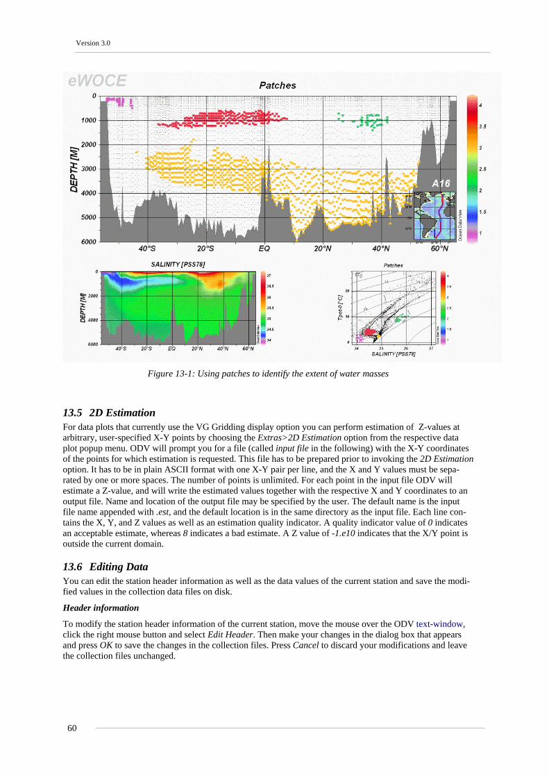
Version 3.0
Figure 13-1: Using patches to identify the extent of water masses
13.5 2D Estimation For data plots that currently use the VG Gridding display option you can perform estimation of Z-values at arbitrary, user-specified X-Y points by choosing the Extras>2D Estimation option from the respective data plot popup menu. ODV will prompt you for a file (called input file in the following) with the X-Y coordinates of the points for which estimation is requested. This file has to be prepared prior to invoking the 2D Estimation option. It has to be in plain ASCII format with one X-Y pair per line, and the X and Y values must be sepa-rated by one or more spaces. The number of points is unlimited. For each point in the input file ODV will estimate a Z-value, and will write the estimated values together with the respective X and Y coordinates to an output file. Name and location of the output file may be specified by the user. The default name is the input file name appended with .est, and the default location is in the same directory as the input file. Each line con-tains the X, Y, and Z values as well as an estimation quality indicator. A quality indicator value of 0 indicates an acceptable estimate, whereas 8 indicates a bad estimate. A Z value of -1.e10 indicates that the X/Y point is outside the current domain.
13.6 Editing Data You can edit the station header information as well as the data values of the current station and save the modi-fied values in the collection data files on disk.
Header information
To modify the station header information of the current station, move the mouse over the ODV text-window, click the right mouse button and select Edit Header. Then make your changes in the dialog box that appears and press OK to save the changes in the collection files. Press Cancel to discard your modifications and leave the collection files unchanged.
60
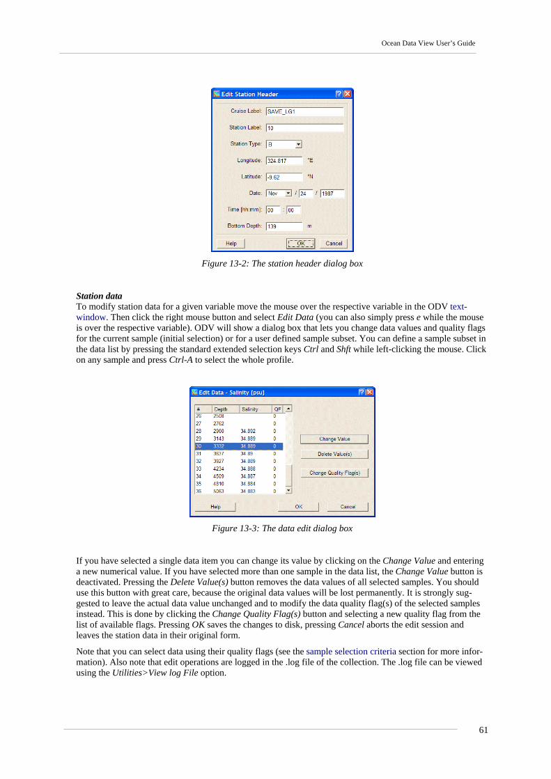
Ocean Data View User’s Guide
Figure 13-2: The station header dialog box
Station data To modify station data for a given variable move the mouse over the respective variable in the ODV text-window. Then click the right mouse button and select Edit Data (you can also simply press e while the mouse is over the respective variable). ODV will show a dialog box that lets you change data values and quality flags for the current sample (initial selection) or for a user defined sample subset. You can define a sample subset in the data list by pressing the standard extended selection keys Ctrl and Shft while left-clicking the mouse. Click on any sample and press Ctrl-A to select the whole profile.
Figure 13-3: The data edit dialog box
If you have selected a single data item you can change its value by clicking on the Change Value and entering a new numerical value. If you have selected more than one sample in the data list, the Change Value button is deactivated. Pressing the Delete Value(s) button removes the data values of all selected samples. You should use this button with great care, because the original data values will be lost permanently. It is strongly sug-gested to leave the actual data value unchanged and to modify the data quality flag(s) of the selected samples instead. This is done by clicking the Change Quality Flag(s) button and selecting a new quality flag from the list of available flags. Pressing OK saves the changes to disk, pressing Cancel aborts the edit session and leaves the station data in their original form.
Note that you can select data using their quality flags (see the sample selection criteria section for more infor-mation). Also note that edit operations are logged in the .log file of the collection. The .log file can be viewed using the Utilities>View log File option.
61

Version 3.0
13.7 Changing the Color Palette You can change the color palette that ODV uses for scatter, section and iso-surface plots using Display Op-tions from the data plot popup menu and selecting one of the available palette files in the Palette combo box. ODV will redraw the data window using the new palette. Note that on high or true color systems you can use different palettes for the different data windows, on systems with only 256 colors all data windows use the same palette (the last one chosen).
On Windows you can create new color palettes or modify existing palettes by means of the PalEdt.exe pro-gram in the ODV binaries directory (normally c:\Program Files\Ocean Data View (mp)\bin_w32). PalEdt.exe can be invoked from ODV by choosing Utilities>Invoke Palette Editor.
ODV-style color palettes define 177 colors: • 0-15: basic colors (used in ODV STATION mode); color 8 used for section topography; • 16-31: gray-scale; color 31 used as background color of ODV plot windows; • 32-144: main palette used for color-shading; • 145-160: colors used for map bathymetry and continents; • 161-176 colors used for map land topography.
13.8 General Settings You can customize general ODV settings such as the graphics and text fonts that ODV uses, or the “good coverage criteria” with the Configuration>General Settings option of the main menu.
Font: Choose a font and various font properties and set the global font scaling factor f. Increase the value for f, if you want larger graphics text and axis annotations, or decrease it otherwise. Note that the more exotic fonts might not be supported in ODV’s PostScript output.
The Text Window>Font Size entry determines the font size used for ODV’s text window, dialog boxes and popup windows.
Canvas: Adjust the width and height of the ODV graphics canvas, e.g., the white area onto which the map and data plots are drawn. Enlarge the graphics canvas if for a maximized ODV window there are gray areas below and/or to the right of the current canvas. Shrink the graphics canvas if for a maximized ODV window there are scroll-bars on the X and/or Y axis of the canvas. Note that you have to exit and restart ODV for size changes to take effect.
Print: Check the Show Collection Info box if you want the ODV time-stamp and collection/configuration info on printouts.
Good Coverage Criteria: Some ODV operations, like for instance interpolation on standard depths or calculation of various derived variables require that there are "sufficient" input data available. Dynamic height, for instance requires tempera-ture and salinity, and the respective profiles should not have too wide data holes. Using the Good Coverage Criteria dialog box you can set and modify the test criteria. These criteria are applied to any variable required for a specific operation. If one or more required variables fail the test, the respective operation is not per-formed.
# Obs number of required observations per station;
Fraction > percentage of samples that must contain data for a given variable;
delta-Z.. specifies the depth dependent tolerable gap between data points.
Program Locations: Enter the full paths of your Web browser (needed for ODV help) and text viewer (needed for viewing text files).
13.9 Data Statistics You can obtain statistics information of the data shown in an arbitrary plot window or the map by using the Extras>Statistics option from the data plot popup menu of the respective plot or from the map popup menu. The window statistics dialog box (see below) will appear and show mean, standard deviation as well as mini-
62

Ocean Data View User’s Guide
mum value and maximum value for the X, Y, and (if present) Z variables of the respective window. Note that mean and standard deviation are calculated using the currently visible data only, while minimum and maxi-mum are based on all available data.
ODV will automatically perform a linear regression of the X and Y data and displays the parameters of the resulting least-squares line. Also shown are the regression coefficient, the root-mean-square difference of the Y data from the line and the total number of data points used for the regression. Note that only the currently displayed data points are used for the regression. You can add the least squares line to the data plot by pressing Show Fit. Note that the line is implemented as a graphics object. You can modify the line style, and you can delete the line when no longer needed.
Figure 13-4: The statistics dialog box
You obtain distribution histograms of the X, Y, and (if present) Z data by pressing on the respective Histogram button. An example histogram is shown below. Note that the histogram is based on the currently visible data only (see example below).
Figure 13-5: A sample data histogram
63

Version 3.0
You obtain a plot of the data distribution in X/Y space by pressing the X/Y Distribution button (see example below: the figure shows the number of XBT temperature profiles from the WOCE Upper Ocean Thermal pro-gramme; data are available from http://www.ewoce.org).
Figure 13-6: A sample data distribution plot
64
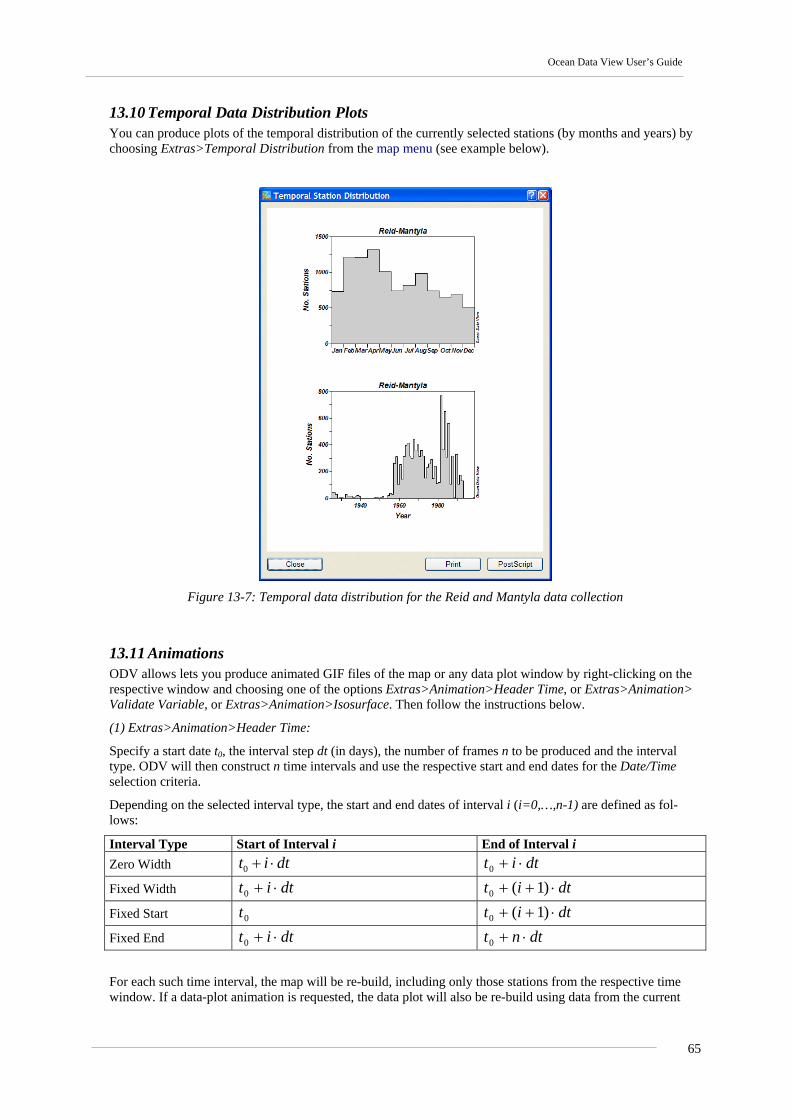
Ocean Data View User’s Guide
13.10 Temporal Data Distribution Plots You can produce plots of the temporal distribution of the currently selected stations (by months and years) by choosing Extras>Temporal Distribution from the map menu (see example below).
Figure 13-7: Temporal data distribution for the Reid and Mantyla data collection
13.11 Animations ODV allows lets you produce animated GIF files of the map or any data plot window by right-clicking on the respective window and choosing one of the options Extras>Animation>Header Time, or Extras>Animation> Validate Variable, or Extras>Animation>Isosurface. Then follow the instructions below.
(1) Extras>Animation>Header Time:
Specify a start date t0, the interval step dt (in days), the number of frames n to be produced and the interval type. ODV will then construct n time intervals and use the respective start and end dates for the Date/Time selection criteria.
Depending on the selected interval type, the start and end dates of interval i (i=0,…,n-1) are defined as fol-lows:
Interval Type Start of Interval i End of Interval i Zero Width dtit ⋅+0 dtit ⋅+0
Fixed Width dtit ⋅+0 dtit ⋅++ )1(0
Fixed Start 0t dtit ⋅++ )1(0
Fixed End dtit ⋅+0 dtnt ⋅+0
For each such time interval, the map will be re-build, including only those stations from the respective time window. If a data-plot animation is requested, the data plot will also be re-build using data from the current
65

Version 3.0
station set only. The current map or data-plot snapshot will then be added to the animation file.
(2) Extras>Animation>Validate Variable:
This option is available for data plot windows only. Select a validate variable and specify a start value v0, the interval step dv, the number of frames n to be produced and the interval type. ODV will then construct n inter-vals for the validate variable and use the respective start and end values for the Validate Variable selection criteria.
Depending on the selected interval type, the start and end values of interval i (i=0,…,n-1) are defined as fol-lows:
Interval Type Start of Interval i End of Interval i Zero Width dviv ⋅+0 dviv ⋅+0
Fixed Width dviv ⋅+0 dviv ⋅++ )1(0
Fixed Start 0v dviv ⋅++ )1(0
Fixed End dviv ⋅+0 dvnv ⋅+0
For each such interval the data-plot will be re-build, including only those data from the respective validate variable interval. The current data-plot snapshot will then be added to the animation file.
(3) Extras>Animation>Isosurface :
This option is available for isosurface data plot windows only. Select a start value s0, the interval step ds, and the number of frames n to be produced. ODV will then construct n isosurface values and will re-build the data-plot window for each such value. The current data-plot snapshot will then be added to the animation file.
For all animations ODV will draw an animation bar indicating the current animation interval. The animation bar is centered below the respective window.
66
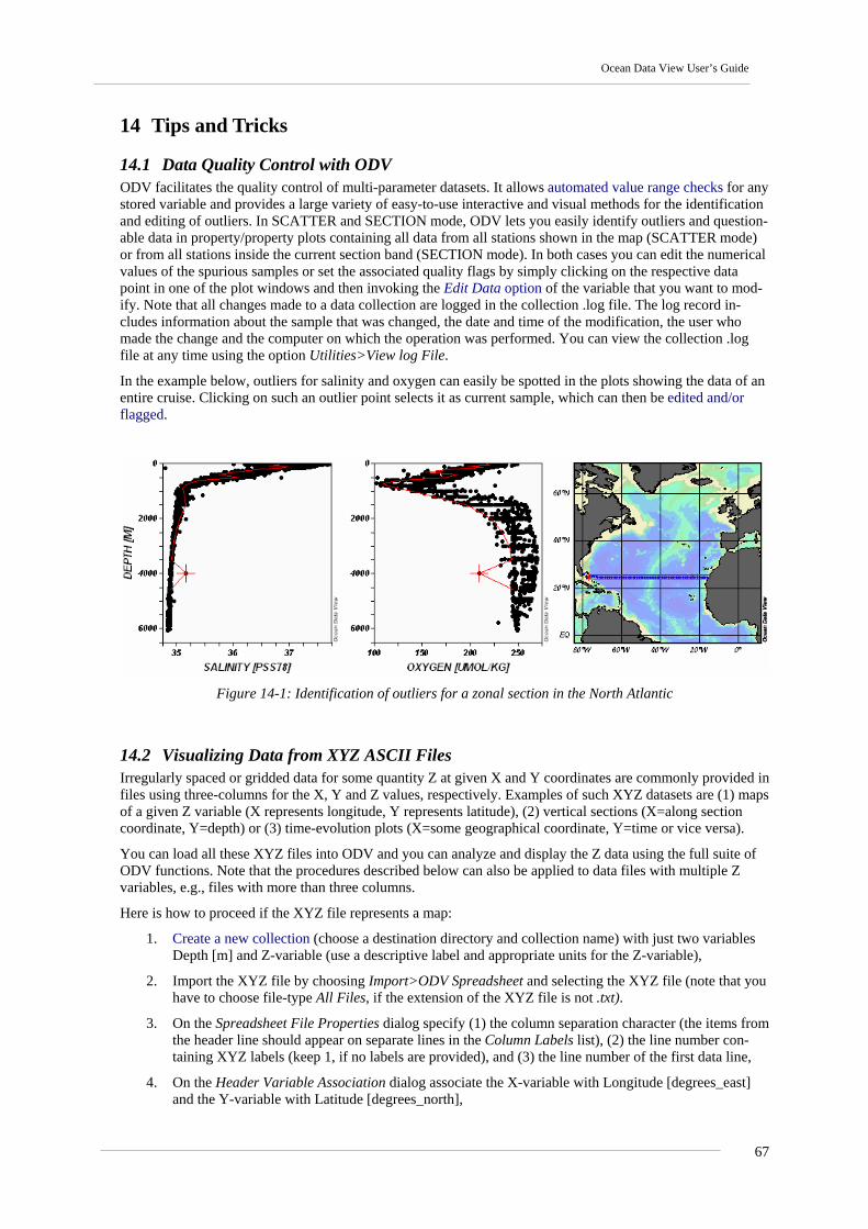
Ocean Data View User’s Guide
14 Tips and Tricks
14.1 Data Quality Control with ODV ODV facilitates the quality control of multi-parameter datasets. It allows automated value range checks for any stored variable and provides a large variety of easy-to-use interactive and visual methods for the identification and editing of outliers. In SCATTER and SECTION mode, ODV lets you easily identify outliers and question-able data in property/property plots containing all data from all stations shown in the map (SCATTER mode) or from all stations inside the current section band (SECTION mode). In both cases you can edit the numerical values of the spurious samples or set the associated quality flags by simply clicking on the respective data point in one of the plot windows and then invoking the Edit Data option of the variable that you want to mod-ify. Note that all changes made to a data collection are logged in the collection .log file. The log record in-cludes information about the sample that was changed, the date and time of the modification, the user who made the change and the computer on which the operation was performed. You can view the collection .log file at any time using the option Utilities>View log File.
In the example below, outliers for salinity and oxygen can easily be spotted in the plots showing the data of an entire cruise. Clicking on such an outlier point selects it as current sample, which can then be edited and/or flagged.
Figure 14-1: Identification of outliers for a zonal section in the North Atlantic
14.2 Visualizing Data from XYZ ASCII Files Irregularly spaced or gridded data for some quantity Z at given X and Y coordinates are commonly provided in files using three-columns for the X, Y and Z values, respectively. Examples of such XYZ datasets are (1) maps of a given Z variable (X represents longitude, Y represents latitude), (2) vertical sections (X=along section coordinate, Y=depth) or (3) time-evolution plots (X=some geographical coordinate, Y=time or vice versa).
You can load all these XYZ files into ODV and you can analyze and display the Z data using the full suite of ODV functions. Note that the procedures described below can also be applied to data files with multiple Z variables, e.g., files with more than three columns.
Here is how to proceed if the XYZ file represents a map:
1. Create a new collection (choose a destination directory and collection name) with just two variables Depth [m] and Z-variable (use a descriptive label and appropriate units for the Z-variable),
2. Import the XYZ file by choosing Import>ODV Spreadsheet and selecting the XYZ file (note that you have to choose file-type All Files, if the extension of the XYZ file is not .txt).
3. On the Spreadsheet File Properties dialog specify (1) the column separation character (the items from the header line should appear on separate lines in the Column Labels list), (2) the line number con-taining XYZ labels (keep 1, if no labels are provided), and (3) the line number of the first data line,
4. On the Header Variable Association dialog associate the X-variable with Longitude [degrees_east] and the Y-variable with Latitude [degrees_north],
67
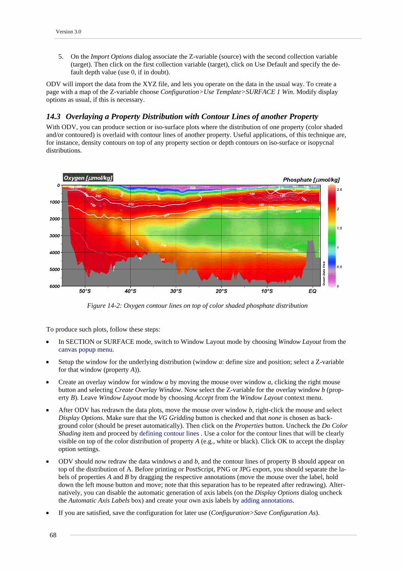
Version 3.0
5. On the Import Options dialog associate the Z-variable (source) with the second collection variable (target). Then click on the first collection variable (target), click on Use Default and specify the de-fault depth value (use 0, if in doubt).
ODV will import the data from the XYZ file, and lets you operate on the data in the usual way. To create a page with a map of the Z-variable choose Configuration>Use Template>SURFACE 1 Win. Modify display options as usual, if this is necessary.
14.3 Overlaying a Property Distribution with Contour Lines of another Property With ODV, you can produce section or iso-surface plots where the distribution of one property (color shaded and/or contoured) is overlaid with contour lines of another property. Useful applications, of this technique are, for instance, density contours on top of any property section or depth contours on iso-surface or isopycnal distributions.
Figure 14-2: Oxygen contour lines on top of color shaded phosphate distribution
To produce such plots, follow these steps:
• In SECTION or SURFACE mode, switch to Window Layout mode by choosing Window Layout from the canvas popup menu.
• Setup the window for the underlying distribution (window a: define size and position; select a Z-variable for that window (property A)).
• Create an overlay window for window a by moving the mouse over window a, clicking the right mouse button and selecting Create Overlay Window. Now select the Z-variable for the overlay window b (prop-erty B). Leave Window Layout mode by choosing Accept from the Window Layout context menu.
• After ODV has redrawn the data plots, move the mouse over window b, right-click the mouse and select Display Options. Make sure that the VG Gridding button is checked and that none is chosen as back-ground color (should be preset automatically). Then click on the Properties button. Uncheck the Do Color Shading item and proceed by defining contour lines . Use a color for the contour lines that will be clearly visible on top of the color distribution of property A (e.g., white or black). Click OK to accept the display option settings.
• ODV should now redraw the data windows a and b, and the contour lines of property B should appear on top of the distribution of A. Before printing or PostScript, PNG or JPG export, you should separate the la-bels of properties A and B by dragging the respective annotations (move the mouse over the label, hold down the left mouse button and move; note that this separation has to be repeated after redrawing). Alter-natively, you can disable the automatic generation of axis labels (on the Display Options dialog uncheck the Automatic Axis Labels box) and create your own axis labels by adding annotations.
• If you are satisfied, save the configuration for later use (Configuration>Save Configuration As).
68
Ocean Data View User’s Guide
Note that for a window entirely overlain by another window (like window a), the only way to access and mod-ify its properties is via the Configuration>Window Properties option from the main menu.
14.4 Pre-computing and Storing Neutral Density Values in Collections Compared to most other derived variables that can be calculated easily and quickly on-the-fly, such as poten-tial temperature, potential density, Brunt-Väisälä Frequency and others, the calculation of neutral density is computationally expensive and relatively time-consuming. While this is not a problem for small data collec-tions or when plotting only a small number of stations, using on-the-fly neutral density calculations with large collections and on long sections can be slow and inefficient. If you are working with large datasets and need neutral density regularly, you should consider to pre-compute neutral density and store the results in collection files on disk. You can then use the pre-computed values from the disk files. Please note that the stored neutral density values need to be re-computed whenever you change depth, temperature and/or salinity values in the collection (e.g., after data edits or calibration changes). It is your responsibility to repeat the neutral density pre-computation described below.
To create a new collection with pre-computed neutral density values for all stations or a station subset of an existing data collection follow these steps:
1. Open the existing collection and select the stations to be included in the new collection with pre-computed neutral density. If you want to process the entire collection, make sure you have a global map and the number of selected stations is identical to the number of stations in the collection (e.g., two numbers at the beginning of line 1 in ODV’s text window should agree).
2. Define Neutral Density as a derived quantity using option Derived Variables from the canvas popup menu.
3. Export the station data including neutral density to an ODV spreadsheet file, by choosing Ex-port>ODV Spreadsheet. Specify a name for the new dataset (denoted as xxx.txt in the following) and make sure that Neutral Density is selected for output in the Select Variables for Output list. The miss-ing value string can be left blank.
4. Use xxx.txt to create a new collection by simply dragging and dropping this file on the ODV desktop icon (Windows and some other platforms) or by starting ODV from a terminal window with “odvmp xxx.txt” (Unix, Linux, Mac OS X). The newly created collection xxx will have Neutral Density as one of its basic variables stored in the disk files.
14.5 Using ODV Graphics in Publications and Web Pages ODV graphics files of the entire ODV canvas or individual data plots can easily be included in print docu-ments, posters or on Web pages.
To create GIF, PNG or JPG files of the entire ODV graphics canvas or of individual plots press Ctrl-s while the mouse is over the canvas or the respective plot window and choose GIF, PNG or JPG as output type. Then specify the desired resolution of the graphics file (default: screen resolution) and use the GIF, PNG or JPG graphics files in your web pages or in text documents. For print documents you can either produce GIF and PNG files with high resolution, or you can use ODV PostScript (.eps) output instead.
A variety of typesetting and page design software supports the import of Encapsulated PostScript files (.eps) in mixed text/graphics pages (e.g., MS Word or compatibles, LaTeX, Adobe PageMaker, etc.). If you use the LaTex typesetting system, see the file Pssample.tex (usually in directory c:\Program Files\Ocean Data View (mp)\Samples) for an example on how to include PostScript graphics in TeX documents. Note that the re-quired epsf and epsfig style files are also included in the samples directory.
If you use Word or PageMaker or other publishing software follow these guidelines: Compose your page as usual and insert the respective ODV PostScript file at the right position. Adjust the size of the figure appropri-ately. When you are done composing the page you can directly print the document on a PostScript printer. If no PostScript printer is available you need to have a PostScript printer-driver and the GhostScript/GhostView package (http://www.cs.wisc.edu/~ghost/aladdin/index.html) installed on your machine. In that case select the PostScript printer-driver as printer and redirect the output into a file. Open this file with GhostView and print to any printer connected to your system.
69

Version 3.0
14.6 Making Cruise Maps You can use ODV to create high quality stations maps for any given data collection using ODV’s MAP mode (all stations or station subsets). Station maps can also be produced, even if you don’t have access to the actual station data but only to the station meta-data (e.g., station postions, etc.). Here is how to proceed:
• In an empty directory on your disk create an ASCII file that will contain the geographic information of your cruise track. This file should have a descriptive name (e.g., CruiseTrack_xxx.txt, where xxx represents the name of your cruise) and it should comply with the generic ODV spreadsheet format specifications.
As first line of the file use the following header line (note that columns are TAB separated): Cruise Station Type mon/day/yr hh:mm Longitude [degrees_east] Latitude [degrees_north] Bot. Depth [m] Dummy1 Dummy2 Immediately following the header line, add one data line for each station or cruise track node and provide the following information for the respective station or node: Cruise The name of the cruise Station Station label or number Type “B” mon/day/yr Station date or current date hh:mm Station time or “00:00” Longitude [degrees_east] Decimal longitude of station Latitude [degrees_north] Decimal latitude of station Bot. Depth [m] Bottom depth at station location or “0” Dummy1 “0” Dummy2 “0”
• On Windows systems drag-and-drop the prepared cruise track file on the ODV(mp) desktop icon; on all other platforms open a terminal window, change directory to the directory containing the cruise track file and start ODV from the terminal window with the cruise track file name as a command line argument (e.g., “odvmp CruiseTrack_xxx.txt”).
• In ODV switch to MAP mode and zoom into the map to define the domain of interest. Specify size and color of the station dots and define the annotation style using the map Display Options. Highlight and annotate specific stations by double-clicking on them or use Extras>Add Graphics Ob-jects>Symbol Sets from map popup menu to highlight and/or connect stations.
• Add new stations to the end of the cruise track .txt file, if necessary, and drag-and-drop the updated cruise track file on the ODV(mp) desktop icon (Windows) or invoke ODV using the cruise track file name as a command line argument (all other platforms).
14.7 Preparing Custom Coastline and Bathymetry Files ODV comes with a coarse resolution global set of coastline and bathymetry files (GlobLR). Higher resolution versions of coast/bathymetry data are available as optional packages for the whole globe (GlobHR) or for selected regions (Baltic, BayOfBiscay, MedHR, and MeditHR). If you need high-resolution representations of coastline and bathymetry for a region not included in the ODV distribution and if you have such high-resolution data available, here is how to produce ODV usable files.
Preparing New Files The data for the coastline and bathymetry contours must be in separate files. Use World.coa as name for the coastline file. The names of the bathymetry files must follow the xxxm.coa scheme, where xxx represents the depth value of the respective contour (no white space between the depth value and the m; example: 1000m.coa). For a sample .coa file see the samples directory of your ODV installation.
The latitude/longitude coordinates of the coastline or depth contour are stored in individual polygon segments (see Figure below). The first nS nodes of a segment represent a part of the actual coastline or bathymetry con-tour. This part of the segment is stroked when the outline of the contour is requested. In addition, each segment can have an optional, second part which will not be stroked but is only used to properly close the segment. Segments that also contain this second part can be filled and/or stroked. The total number nT of nodes in any segment must not exceed 1500. If a segment has no second part, the number of stroke points nS must be equal to nT.
70
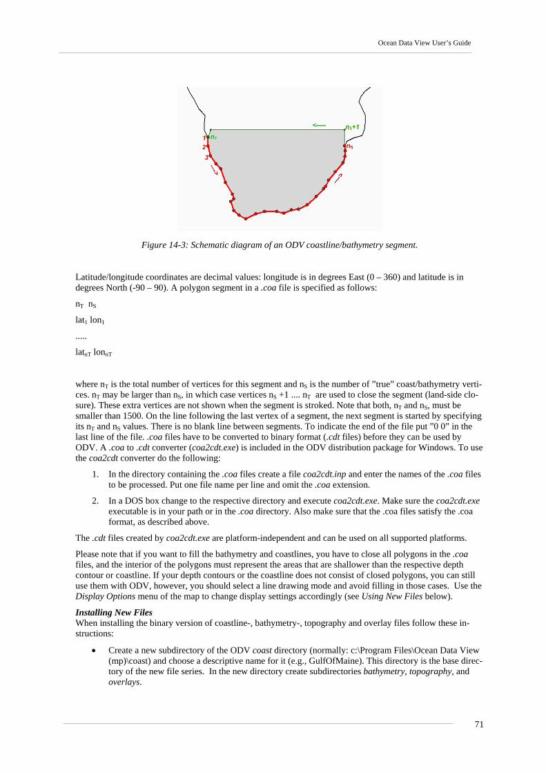
Ocean Data View User’s Guide
Figure 14-3: Schematic diagram of an ODV coastline/bathymetry segment.
Latitude/longitude coordinates are decimal values: longitude is in degrees East (0 – 360) and latitude is in degrees North (-90 – 90). A polygon segment in a .coa file is specified as follows:
nT nS
lat1 lon1
.....
latnT lonnT
where nT is the total number of vertices for this segment and nS is the number of ”true” coast/bathymetry verti-ces. nT may be larger than nS, in which case vertices nS +1 .... nT are used to close the segment (land-side clo-sure). These extra vertices are not shown when the segment is stroked. Note that both, nT and nS, must be smaller than 1500. On the line following the last vertex of a segment, the next segment is started by specifying its nT and nS values. There is no blank line between segments. To indicate the end of the file put ”0 0” in the last line of the file. .coa files have to be converted to binary format (.cdt files) before they can be used by ODV. A .coa to .cdt converter (coa2cdt.exe) is included in the ODV distribution package for Windows. To use the coa2cdt converter do the following:
1. In the directory containing the .coa files create a file coa2cdt.inp and enter the names of the .coa files to be processed. Put one file name per line and omit the .coa extension.
2. In a DOS box change to the respective directory and execute coa2cdt.exe. Make sure the coa2cdt.exe executable is in your path or in the .coa directory. Also make sure that the .coa files satisfy the .coa format, as described above.
The .cdt files created by coa2cdt.exe are platform-independent and can be used on all supported platforms.
Please note that if you want to fill the bathymetry and coastlines, you have to close all polygons in the .coa files, and the interior of the polygons must represent the areas that are shallower than the respective depth contour or coastline. If your depth contours or the coastline does not consist of closed polygons, you can still use them with ODV, however, you should select a line drawing mode and avoid filling in those cases. Use the Display Options menu of the map to change display settings accordingly (see Using New Files below).
Installing New Files When installing the binary version of coastline-, bathymetry-, topography and overlay files follow these in-structions:
• Create a new subdirectory of the ODV coast directory (normally: c:\Program Files\Ocean Data View (mp)\coast) and choose a descriptive name for it (e.g., GulfOfMaine). This directory is the base direc-tory of the new file series. In the new directory create subdirectories bathymetry, topography, and overlays.
71
Version 3.0
• Copy the coastline file (normally called World.cdt) into the series base directory (e.g., c:\Program Files\Ocean Data View (mp)\coast\ GulfOfMaine).
• Copy all bathymetry files (e.g., 100m.cdt, 500m.cdt, etc.) into the bathymetry subdirectory, all topog-raphy files into the topography directory and all general purpose overlay files (rivers, lakes, borders, etc.) into the overlays directory. If no topography and/or overlay files are available the respective di-rectories remain empty.
Using New Files To use the newly installed files in ODV maps do the following:
• Invoke the map Display Options dialog box (e.g., right-click the mouse while over the map and choose Display Options) and select the Layers tab.
• Choose the newly installed series name (e.g., GulfOfMaine) in the Series combo-box.
• Compose the layer-set(s) of interest by selecting a layer-set (e.g., Ocean Bathymetry) and then press-ing Compose. Select the contour files that you want to use in the Available list, set the desired stroke and fill properties and finally press << to add the files to the Selected list (note: if you forget to press << no file is added). To remove files from the Selected list select them and press >>.
When specifying drawing characteristics follow these rules:
(a) If the features should be outlined by lines (stroked), choose the appropriate line-width, -type and –color or choose none as color, if you don’t want outlines. Note that due to limitations of the op-erating system, on some Windows versions thick lines will always be drawn as solid lines on the screen and in GIF, PNG and JPG output files. ODV PostScript files, however, honor your selec-tion for any line-width.
(b) If the features should be filled choose the appropriate Fill color or none, if you don’t want filling.
If you choose automatic for line and fill colors, ODV will use default colors. Note that for some layer sets automatic defaults to none. Also note that some feature files like rivers or borders should not be filled and you should explicitly set the fill color to none.
ODV processes the layer sets in the order as listed in the Display Options dialog box. For a given layer set it draws the individual layers in the order in which they appear in the Selected list (note that ocean bathymetry and land topography layers are sorted automatically when they are added). You should define sea-ice distribu-tions in the pre-Coastlines set and lakes, rivers and borders in the post-Topography category.
72

Ocean Data View User’s Guide
15 Appendix
15.1 ODV Directory Structure The default installation directory for ODV is c:\Program Files\Ocean Data View (mp) on Windows and /usr/local/odvmp for UNIX (indicated as <odv_root> below; for UNIX replace \ by / in the following). The installation directory is the root for a number of subdirectories containing files of specific type. Installation files that may be modified by the user, such as macro files, palette files or sample data collections, are installed in subdirectory odv_local under the user’s home directory (indicated as <home>).
<odv_root>\bin_w32 on Windows platforms, ...or... <odv_root>\bin_linux-i386 on Linux i386 platforms, ...or... <odv_root>\bin_solaris-sparc on SUN Solaris Sparc platforms, ...or... <odv_root>\bin_irix6.5_mips on SGI Irix platforms, ...or... <odv_root>\bin_aix-powerpc on IBM AIX powerpc platforms, ...or... <odv_root>\bin_macx on Mac OS X platforms:
ODV executable, help files, and PostScript preamble file.
<odv_root>\coast\GlobLR: Low-resolution coastline and topography files for the whole globe.
<odv_root>\coast\GlobHR: High-resolution coastline and topography files for the whole globe (available as optional package).
<odv_root>\doc: ODV html help files (pdf version available from ODV web page).
<odv_root>\include: Default directory for ODV include files (e.g., ETOPO2 global topography available as optional package). Note that there are several sub-directories containing other files of a given type.
<odv_root>\include\atmhist: Concentration histories of various atmospheric trace gases.
<odv_root>\include\gazetteers: ODV gazetteer database files.
<odv_root>\samples: Directory for ODV sample files. Use these files as templates for data import or macro files.
<home>\odv_local\data: Default base-directory for ODV data collections. You can place your data collections anywhere on disk or CD-ROM, however, it is recommended that you create individual sub-directories for every collection that you maintain.
<home>\odv_local\data\SAVE: Sample ODV data collection containing the South Atlantic Ventilation Experiment data.
<home>\odv_local\include\macros: ODV macro files (.mac).
<home>\odv_local\include\palettes: ODV palette files (.pal).
User’s default Temp directory: Directory for temporary files. Files with names starting with ODV are routinely removed from this directory, if they are older than 3 days.
15.2 Quality Flag Mapping During data import, ODV converts data quality flags found in the import files to corresponding ODV quality
73
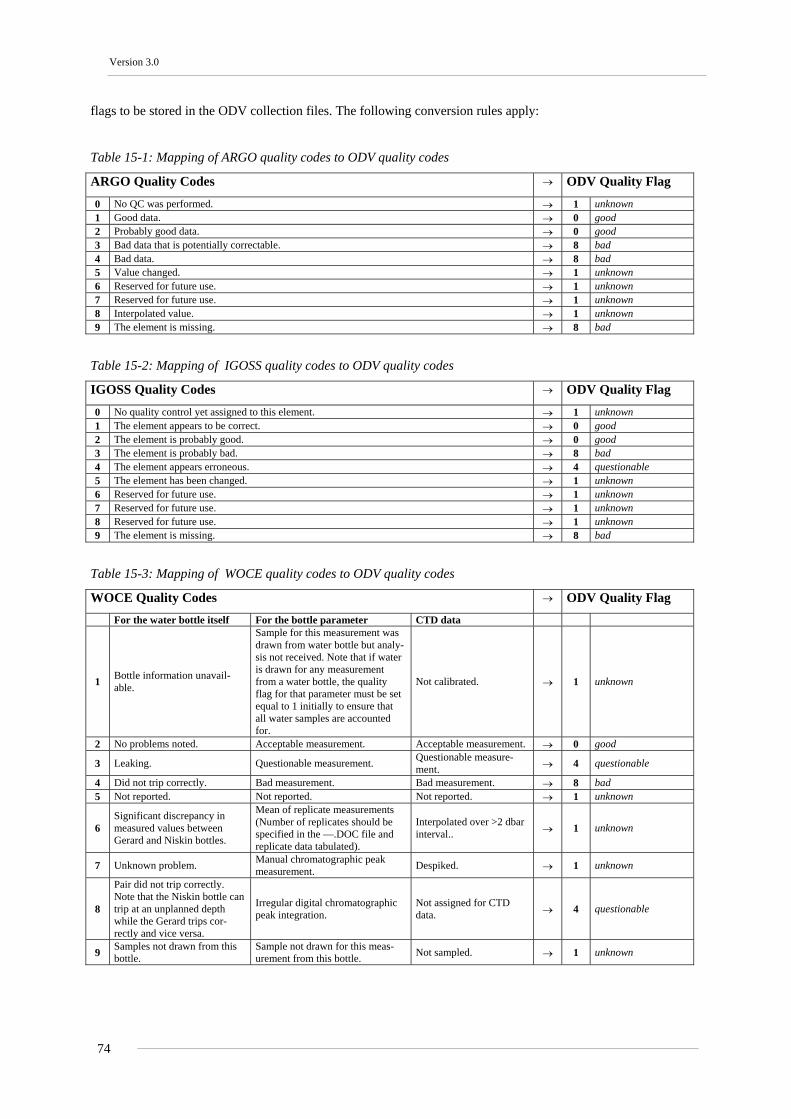
Version 3.0
flags to be stored in the ODV collection files. The following conversion rules apply:
Table 15-1: Mapping of ARGO quality codes to ODV quality codes
ARGO Quality Codes → ODV Quality Flag
0 No QC was performed. → 1 unknown 1 Good data. → 0 good 2 Probably good data. → 0 good 3 Bad data that is potentially correctable. → 8 bad 4 Bad data. → 8 bad 5 Value changed. → 1 unknown 6 Reserved for future use. → 1 unknown 7 Reserved for future use. → 1 unknown 8 Interpolated value. → 1 unknown 9 The element is missing. → 8 bad
Table 15-2: Mapping of IGOSS quality codes to ODV quality codes
IGOSS Quality Codes → ODV Quality Flag
0 No quality control yet assigned to this element. → 1 unknown 1 The element appears to be correct. → 0 good 2 The element is probably good. → 0 good 3 The element is probably bad. → 8 bad 4 The element appears erroneous. → 4 questionable 5 The element has been changed. → 1 unknown 6 Reserved for future use. → 1 unknown 7 Reserved for future use. → 1 unknown 8 Reserved for future use. → 1 unknown 9 The element is missing. → 8 bad
Table 15-3: Mapping of WOCE quality codes to ODV quality codes
WOCE Quality Codes → ODV Quality Flag For the water bottle itself For the bottle parameter CTD data
1 Bottle information unavail-able.
Sample for this measurement was drawn from water bottle but analy-sis not received. Note that if water is drawn for any measurement from a water bottle, the quality flag for that parameter must be set equal to 1 initially to ensure that all water samples are accounted for.
Not calibrated. → 1 unknown
2 No problems noted. Acceptable measurement. Acceptable measurement. → 0 good
3 Leaking. Questionable measurement. Questionable measure-ment. → 4 questionable
4 Did not trip correctly. Bad measurement. Bad measurement. → 8 bad 5 Not reported. Not reported. Not reported. → 1 unknown
6 Significant discrepancy in measured values between Gerard and Niskin bottles.
Mean of replicate measurements (Number of replicates should be specified in the —.DOC file and replicate data tabulated).
Interpolated over >2 dbar interval.. → 1 unknown
7 Unknown problem. Manual chromatographic peak measurement. Despiked. → 1 unknown
8
Pair did not trip correctly. Note that the Niskin bottle can trip at an unplanned depth while the Gerard trips cor-rectly and vice versa.
Irregular digital chromatographic peak integration.
Not assigned for CTD data. → 4 questionable
9 Samples not drawn from this bottle.
Sample not drawn for this meas-urement from this bottle. Not sampled. → 1 unknown
74

Ocean Data View User’s Guide
Table 15-4: Mapping of WOD01 “entire station” quality codes to ODV quality codes
World Ocean Database 2001 Quality Codes → ODV Quality Flag Entire station Individual depth observations
0 accepted station. accepted value. → 0 good
1 failed annual standard deviation check. duplicates or inversions in recorded depth (same or less than previous depth). → 4 questionable
2 two or more density inversions (Levitus, 1982 criteria). density inversion → 4 questionable
3 flagged cruise. → 4 questionable 4 failed seasonal standard deviation check. → 4 questionable 5 failed monthly standard deviation check. → 4 questionable 6 flag 1 and flag 4. → 4 questionable
7 bullseye from standard level data or failed annual and monthly standard deviation check. → 4 questionable
8 failed seasonal and monthly standard deviation check. → 4 questionable
9 failed annual, seasonal and monthly standard deviation check. → 4 questionable
Table 15-5: Mapping of WOD01 “individual observed-level” quality codes to ODV quality codes
World Ocean Database 2001 Quality Codes → ODV Quality Flag Individual observed-level parameters
0 accepted value. → 0 good 1 range outlier (outside of broad range check). → 4 questionable 2 failed inversion check. → 4 questionable 3 failed gradient check. → 4 questionable 4 observed level "bullseye" flag and zero gradient check. → 4 questionable 5 combined gradient and inversion checks. → 4 questionable 6 failed range and inversion checks. → 8 bad 7 failed range and gradient checks. → 8 bad 8 failed range and questionable data checks. → 8 bad 9 failed range and combined gradient and inversion checks. → 8 bad
If WOD “entire station” and “individual observed sample” flags are available, ODV maps the two values to ODV quality flags separately, and then uses the maximum of the two ODV flags as the quality flag of the sample.
15.3 Generic ODV Spreadsheet Format
The ODV generic spreadsheet format is the preferred exchange format for import of data into ODV collections and for data export from ODV collections. It allows for automatic data exchange and requires no user interac-tion.
Category Specification
General ASCII coding
File extension .txt
Comment lines Start with // as first two characters (comment lines are added to the collection .info file during import). Comment lines may appear anywhere in the file.
Columns Station header information (metadata) and data values for up to 50 variables are stored in separate columns. Header and data columns can be in arbitrary order. All non-comment lines in the file must have the same number of columns.
Column separation character TAB or ;
Header Line (first non-comment line; must be present)
1. Contains column labels.
2. The following metadata header labels must be used exactly as given below: "Cruise", "Station", "Type", "mon/day/yr", "hh:mm", "Longitude
75
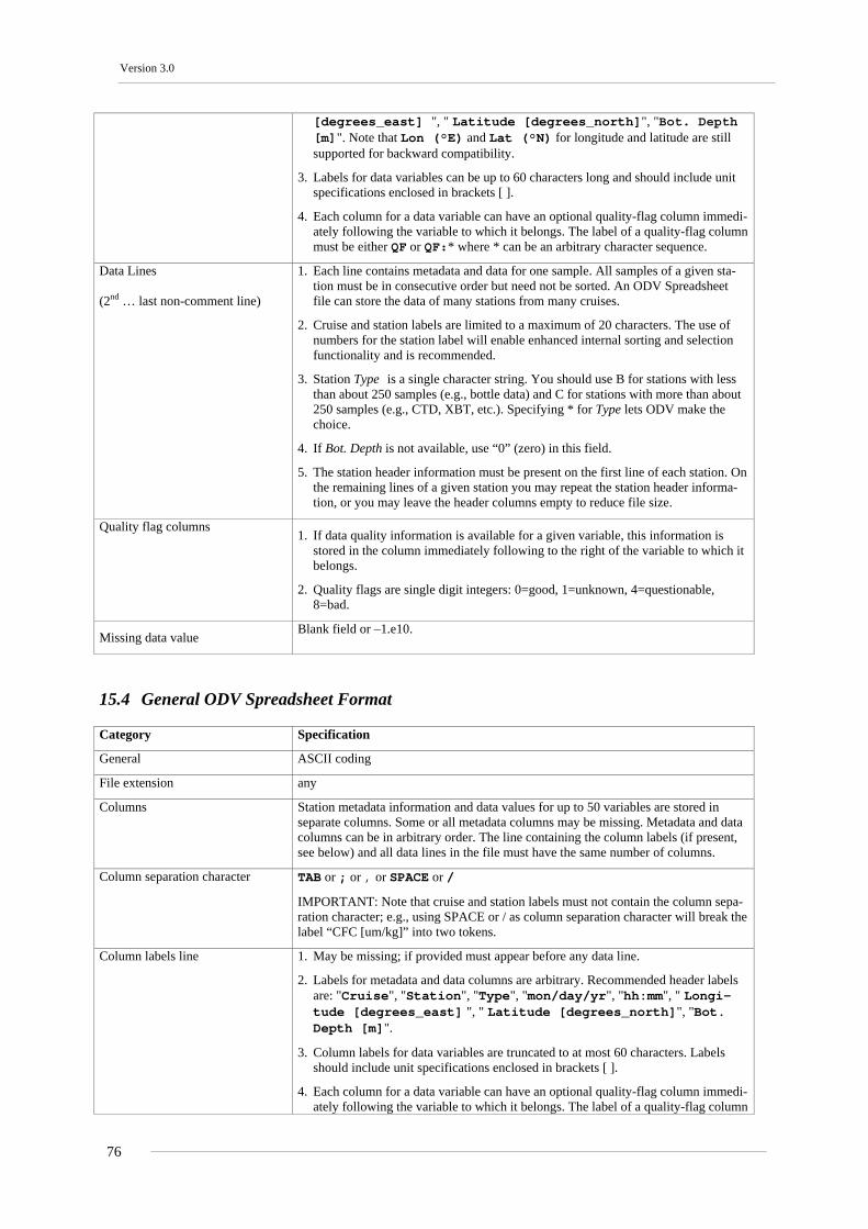
Version 3.0
[degrees_east] ", " Latitude [degrees_north]", "Bot. Depth [m]". Note that Lon (°E) and Lat (°N) for longitude and latitude are still supported for backward compatibility.
3. Labels for data variables can be up to 60 characters long and should include unit specifications enclosed in brackets [ ].
4. Each column for a data variable can have an optional quality-flag column immedi-ately following the variable to which it belongs. The label of a quality-flag column must be either QF or QF:* where * can be an arbitrary character sequence.
Data Lines (2nd … last non-comment line)
1. Each line contains metadata and data for one sample. All samples of a given sta-tion must be in consecutive order but need not be sorted. An ODV Spreadsheet file can store the data of many stations from many cruises.
2. Cruise and station labels are limited to a maximum of 20 characters. The use of numbers for the station label will enable enhanced internal sorting and selection functionality and is recommended.
3. Station Type is a single character string. You should use B for stations with less than about 250 samples (e.g., bottle data) and C for stations with more than about 250 samples (e.g., CTD, XBT, etc.). Specifying * for Type lets ODV make the choice.
4. If Bot. Depth is not available, use “0” (zero) in this field.
5. The station header information must be present on the first line of each station. On the remaining lines of a given station you may repeat the station header informa-tion, or you may leave the header columns empty to reduce file size.
Quality flag columns 1. If data quality information is available for a given variable, this information is
stored in the column immediately following to the right of the variable to which it belongs.
2. Quality flags are single digit integers: 0=good, 1=unknown, 4=questionable, 8=bad.
Missing data value Blank field or –1.e10.
15.4 General ODV Spreadsheet Format
Category Specification
General ASCII coding
File extension any
Columns Station metadata information and data values for up to 50 variables are stored in separate columns. Some or all metadata columns may be missing. Metadata and data columns can be in arbitrary order. The line containing the column labels (if present, see below) and all data lines in the file must have the same number of columns.
Column separation character TAB or ; or , or SPACE or /
IMPORTANT: Note that cruise and station labels must not contain the column sepa-ration character; e.g., using SPACE or / as column separation character will break the label “CFC [um/kg]” into two tokens.
Column labels line 1. May be missing; if provided must appear before any data line.
2. Labels for metadata and data columns are arbitrary. Recommended header labels are: "Cruise", "Station", "Type", "mon/day/yr", "hh:mm", " Longi-tude [degrees_east] ", " Latitude [degrees_north]", "Bot. Depth [m]".
3. Column labels for data variables are truncated to at most 60 characters. Labels should include unit specifications enclosed in brackets [ ].
4. Each column for a data variable can have an optional quality-flag column immedi-ately following the variable to which it belongs. The label of a quality-flag column
76

Ocean Data View User’s Guide
must be either QF or QF:* where * represents an arbitrary character sequence.
Data lines 1. May start at any line of the file. All lines following the first data line are assumed to be data lines as well (no comments at the end of the file!).
2. Each line contains metadata and data for one sample. All samples of a given sta-tion must be in consecutive order but need not be sorted. An ODV spreadsheet file can store the data of many stations from many cruises.
3. Station Type is a single character string (use B for stations with less than 250 samples (e.g., bottle data) and C for stations with more than about 250 samples (e.g., CTD, XBT, etc.). Specifying * for Type lets ODV make the choice.
4. If Bot. Depth is not available, use “0” (zero) in this field.
5. The station header information (if header columns are included) must be present on all lines.
Quality flag columns 1. If data quality information is available for a given variable, this information is
stored in the column immediately following to the right of the variable to which it belongs.
2. Quality flags are single digit integers. They must be one of the following: 0=good, 1=unknown, 4=questionable, 8=bad.
Missing data value Blank field or any numerical value beyond the range of good data.
15.5 o4x Exchange Format ODV .o4x exchange files contain information on the type of the data, the number and labels of variables, the actual data values and the data quality flags in a single ASCII file with extension .o4x. Typically, .o4x files contain three sections: (1) a (possibly missing) comment section consisting of an arbitrary number of free-format lines of at most 200 characters each (this part may be missing), (2) a variables section that describes the type of the data and the number and labels of variables in the file, and (3) the data section that contains the actual data values and data quality flags. Data quality flags may be missing; if they appear they must be single digit ODV quality flags. For a sample .o4x file see the samples directory of your ODV installation.
The .o4x variables section begins with the keyword ODV4.0 Listing and should be formatted as shown in the sample below. Any records before the ODV4.0 Listing line are treated as comments and will be added to the collection .info file during import.
Sample .o4x variables section (Note that the "....+." lines at the top and bottom only serve as rulers and are not part of the file.) ....+....1....+....2....+....3....+....4....+....5....+....6.... ODV4.0 Listing File Name: import4.o4x Type: HYD Nstat: 12 Variables: 8 Depth [m] 6.0 Temperature [°C] 8.2 Salinity [psu] 8.3 Oxygen [~$m~#mol/kg] 6.0 Phosphate [~$m~#mol/kg] 8.2 Silicate [~$m~#mol/kg] 8.1 Nitrate [~$m~#mol/kg] 7.1 Nitrite [~$m~#mol/kg] 6.1 ....+....1....+....2....+....3....+....4....+....5....+....6....
One empty line separates the variables section of the data file from the header line of the first station (see file import4.o4x in the ODV samples directory for an example). Station header lines must start with a # in column 1. The following items are: (1) cruise-label of the station (cols. [3:22], format a20); (2) station-label ([24:43], a20); (3) station-type (either B, C or X for bottle, CTD or XBT data; [45:45], a1); (4) date mm/dd/yyyy
77

Version 3.0
([47:66], i2,1x,i2,1x,i4); (5) east longitude (decimal; [58:64], f7.3); (6) north latitude (decimal; [66:72], f7.3); (7) bottom depth ([m]; [74:78], i5); (8) depth of deepest observation ([m]; [80:84], i5); (9) number of depths sampled ([85:89], i5); (10) number of variables for which data are provided in the file ([91:93], i3). In the example file, the station 06MT18/558 is of type "Bottle", it contains 14 observed depths and data for 8 vari-ables at these observed depths are to follow. These variables have to be identified by specifying their numbers (as defined in the variables section at the beginning of the file) on the second header line (e.g., 1 represents Depth and, for instance, 6 represents Silicate). Note that as the only format restriction, the variable numbers on the second header line have to be separated by at least one blank.
For each observed depth (14 in the example file) one line of data has to follow. Each of these lines must con-tain a data and quality flag value for every variable specified on the second header line in that order. Missing values have to be set to -1.000E+10 in the data file. Note that data and quality flag values have to be separated by at least one space. Quality flags are single digit integers with the following meaning: 0=Good, 1=Unknown, 4=Questionable, 8=Bad. Immediately after the last data line of a given station follows the first header line (starting with the #) of the next station to be imported or the end-of-file if the station is the last to be read.
Once the.o4x file has been created, start ODV and open or create the collection that is to receive the new data. Then choose ODV4.x Listing from the Import menu. Select the ASCII data file created above as data import file. Specify import options and press OK to start the data import. ODV will then read the import file and add/merge the stations to the collection. Note that you can also drag-and-drop .o4x files onto ODV.
15.6 o3x Exchange Format To import data using the .o3x exchange format you have to provide two ASCII files, one containing the actual data for all the stations that you want to import (default extension is .o3x) and one (small) file that describes the variables included in the data file (extension must be .var). For a sample .o3x file see the samples directory of your ODV installation.
Sample .var File ....+....1....+....2....+....3....+....4....+....5....+....6.... ODV4.0 Collection: SAVE Type: HYD Nstat: 0 Variables: 7 Depth [m] 6.0 Temperature [°C] 8.2 Salinity [psu] 8.3 Oxygen [~$m~#mol/kg] 6.0 Phosphate [~$m~#mol/kg] 8.2 Silicate [~$m~#mol/kg] 8.1 Nitrate [~$m~#mol/kg] 7.1 ....+....1....+....2....+....3....+....4....+....5....+....6....
Note that the “....+.” lines at the top and bottom only serve as rulers and are not part of the .var file. Also note that the .var file has the same format as ODV4.x collection definition files but that the information needed for the data import is confined to entries concerning the variables. In line 5 of the file starting in column 13 you have to specify the number of variables included in the data file to be imported. Then, after one blank line you have to provide variable label and numeric format for all the variables on separate lines. The numeric format has the appearance ll.d (ll is the total length in characters and d is the number of decimal figures) and starts in column 61.
Sample .o3x header lines ....+....1....+....2....+....3....+....4....+....5....+....6....+....7... # REID_ET 212 B 6/21/1967 243.167 -28.233 3400 3310 34 7 1 2 3 4 5 6 7
The data for all the stations to be imported have to be provided in a single ASCII file (default extension .o3x). This file has to meet the following format specification (note that the ruler at the top is not part of the file):
The file must begin with the header line of the first station to be imported. Station header lines must start with a # in column 1. The following items are: (1) cruise-label of the station (cols. [3:12], format a10); (2) station-
78

Ocean Data View User’s Guide
label ([14:23], a10); (3) station-type (either B, C or X for bottle, CTD or XBT data; [25:25], a1); (4) date mm/dd/yyyy ([27:36], i2,1x,i2,1x,i4); (5) east longitude (decimal; [38:44], f7.3); (6) north latitude (decimal; [46:52], f7.3); (7) bottom depth ([m]; [54:58], i5); (8) depth of deepest observation ([m]; [60:64], i5); (9) num-ber of depths sampled ([66:69], i4); (10) number of variables for which data are provided in the file ([71:73], i3). In the example above, the station REID_ET/212 is of type “Bottle”, it contains 34 observed depths and data for 7 variables at these observed depths are to follow. These variables have to be identified by specifying their numbers as defined in the .var file on the second header line (e.g., 1 represents Depth and, for instance, 6 represents Silicate). Note that as the only format restriction, the variable numbers on the second header line have to be separated by at least one blank.
For each observed depth (34 in the example above) one line of data has to follow. Each of these lines must contain a numerical value for every variable specified on the second header line in that order. Missing values have to be set to -1.000E+10 in the data file. Immediately after the last data line of a given station follows the first header line (starting with the #) of the next station to be imported or the end-of-file if the station is the last to be read.
Once the .var and .o3x files have been created, run ODV and open or create the collection that is to receive the new data. Then choose ODV3.0 Listing from the Import menu. Select the ASCII data file created above as data import file and identify the variables to be imported by selecting the import .var file as the data source. Specify import options and press OK to start the data import. ODV will then read the import file and add/merge the stations to the collection. Note that the data quality flags are set to Unknown if you import data using ODV3.0 exchange format.
15.7 Control Sequences and Functions in ODV Annotations Table 15-6: Formatting control sequences in ODV annotations.
Control Sequence Result
~$ Switches to Symbol font (Greek symbols)
~# Switches to normal text font
~% Produces per mille character (‰)
~^ Next character drawn as superscript
~_ Next character drawn as subscript.
Example: “~$S~#CO~_2 [~$m~#mol/kg” will produce ΣCO2 [µmol/kg].
Table 15-7: Available auto-functions in ODV annotations.
Function Substituted Text
=date() Current date
=time() Current time
=user() User and host name
=collection() Full path of current collection
=cfg_file() Full path of current configuration file
=sec_file() Full path of current section file
15.8 Hardware Requirements and Limitations The multi-platform version of ODV runs on computers with the Windows (9x/Me/NT/2000/XP), Linux, Mac OS X, and various UNIX operating systems. Note that on some systems administrator privileges are required to install ODV.
The hardcopy routines of ODV have been tested on black white and color Apple LaserWriter, Canon Laser
79
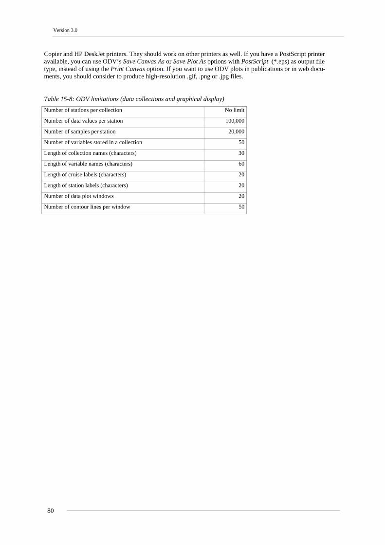
Version 3.0
Copier and HP DeskJet printers. They should work on other printers as well. If you have a PostScript printer available, you can use ODV’s Save Canvas As or Save Plot As options with PostScript (*.eps) as output file type, instead of using the Print Canvas option. If you want to use ODV plots in publications or in web docu-ments, you should consider to produce high-resolution .gif, .png or .jpg files.
Table 15-8: ODV limitations (data collections and graphical display)
Number of stations per collection No limit
Number of data values per station 100,000
Number of samples per station 20,000
Number of variables stored in a collection 50
Length of collection names (characters) 30
Length of variable names (characters) 60
Length of cruise labels (characters) 20
Length of station labels (characters) 20
Number of data plot windows 20
Number of contour lines per window 50
80