Occupation-industry mismatch in the cross-section and the aggregate

Saman Darougheh sdma@nationalbanken.dk

DANMARKS NATIONALBANK

The Working Papers of Danmarks Nationalbank describe research and development, often still ongoing, as a contribution to the professional debate.

The viewpoints and conclusions stated are the responsibility of the individual contributors, and do not necessarily reflect the views of Danmarks Nationalbank.

2 2 NO V E M B E R 2 01 9 — N O . 1 4 7

W O R K I N G P A P E R — D A N M AR K S N A T IO N A L B A N K

2 2 NO V E M B E R 2 01 9 — N O . 1 4 7

Abstract I define occupations that are employed in more industries as “broader” occupations. I study the implications of broadness for mismatch of the unemployed and vacancies across occupations and industries. I empirically find that workers in broader occupations are better insured against industry-specific shocks. A recent literature has found that mismatch did not significantly contribute to the rise in unemployment during the Great Recession. I build a general equilibrium model that uses occupational broadness as a microfoundation of mismatch. The model uncovers a general equilibrium channel that realigns the strong cross-sectional effects of mismatch with its missing aggregate impact. I argue that mismatch across occupations and industries cannot significantly contribute to aggregate unemployment fluctuations.

Resume Jeg definerer erhvervsgrupper, der dækker flere brancher, som “bredere” erhvervsgrupper. Jeg undersøger på erhvervsgruppeniveau breddens konsekvenser for mismatch mellem ledige arbejdstagere og ledige stillinger på tværs af erhvervsgrupper og brancher. Jeg finder empirisk belæg for, at arbejdstagere i bredere erhvervsgrupper er bedre forsikret mod branchespecifikke stød. Nyere litteratur viser dog, at mismatch ikke bidrog signifikant til stigningen i ledigheden under den sidste recession. Jeg konstruerer en generel ligevægtsmodel, der bruger erhvervsgruppernes bredde som en et mikrofundament for mismatch. Modellen viser en generel ligevægtskanal, som forener de stærke tværsnitseffekter af mismatch med den manglende effekt på aggregeret niveau. Jeg argumenterer for, at mismatch på tværs af erhvervsgrupper og brancher ikke kan bidrage signifikant fluktuationer i den aggregerede ledighed.

Occupation-industry mismatch in the cross-section and the aggregate

Acknowledgements The authors wish to thank colleagues from Danmarks Nationalbank. The authors alone are responsible for any remaining errors.

Key words Macroeconomics, labor economics, unemployment, mismatch JEL classification E24; J22; J24; J63; J64

Occupation-industry mismatch in the cross-section and theaggregate*

Saman Darougheh†

is version: November 15, 2019

Abstract

I dene occupations that are employed in more industries as “broader” occupations. I studythe implications of broadness for mismatch of unemployed and vacancies across occupationsand industries. I empirically nd that workers in broader occupations are better insured againstindustry-specic shocks. A recent literature has found that mismatch did not signicantly con-tribute to the rise in unemployment during the Great Recession. To explain the seeming con-tradiction between the impact of mismatch on individual unemployment risk and aggregateunemployment outcomes, I build a general equilibriummodel that uses occupational broadnessas a microfoundation of mismatch. e model uncovers an important general equilibrium chan-nel that realigns the strong cross-sectional eects of mismatch with its missing aggregate impact.I conclude that mismatch across occupations and industries cannot signicantly contribute toaggregate unemployment uctuations. (JEL E24, J22, J24, J63, J64)

*Previously circulated under the title “Specialized human capital and unemployment”. I am indebted tomy advisors PerKrusell and Kurt Mitman. I also thank Almut Balleer, Mark Bils, Tobias Broer, Gabriel Chodorow-Reich, Mitch Downey,Richard Foltyn, Karl Harmenberg, Erik Hurst, Gregor Jarosch, Hamish Low, Hannes Malmberg, Kaveh Majlesi, GiuseppeMoscarini, Arash Nekoei, Erik Oberg, Jonna Olsson, Torsten Persson, Morten Ravn, Aysegul Sahin, Josef Sigurdsson,David Stromberg, Ludo Visschers, and numerous seminar participants for their comments.

†Danmarks Nationalbank. E-mail: s.darougheh@gmail.com.

1

1 Introduction

Between and , the United States experienced one of the largest downturns in the post-warera. During that period, the US unemployment rate increased from .% to %. Simultaneously,the job-nding rate decreased persistently and the Beveridge curve shied outwards – the samenumber of vacancies and unemployed workers led to fewer hires than before. One explanation forthis dramatic disruption of the labormarket is “mismatch unemployment” – the idea that job seekersmay be of a dierent type than what rms are looking for.ere aremanypotential dimensions ofmismatch, and they all require some friction that prevents

job seekers from adjusting to the requirements of the vacancies. To see which dimensions are mostimportant in explaining unemployment, I carry out an empirical investigation that lets the dataspeak without imposing any structural assumptions. I perform a machine learning exercise wherethe individual unemployment status is predicted out of sample using independent variables from theCPS. I nd that an individual’s occupation and industry are among the most important predictorsof their unemployment status.1is is in line with the notion of mismatch: human capital that isspecic to occupations or industries might impede the unemployed from changing labor markets.If shocks aect occupations and industry asymmetrically, an individual’s current occupation andindustry will be an important determinant of their unemployment risk.It is a well-known hypothesis that industries are aected unequally by aggregate business cycles

(Lilien, 1982), and that the Great Recession aected some industries more than others. As for oc-cupations, the sharp increase in unemployment during the Great Recession was accompanied bya rise in the dispersion of occupation-specic unemployment rates, as displayed in Figure 1. Forexample, the unemployment rate of construction-related occupations increased by up to percent-age points, whereas it increased by less than percentage points in many other occupations. isdierential impact of the recession by occupation could potentially be explained by the industriesthat employ workers in these occupations: construction-related occupations have larger unemploy-ment responses because the construction industry faced a large downturn during the recession. eright-hand panel shows that this is not the case: I residualize the individual-level unemploymentstatus with individual demographics and full interactions of industry, state and year. Yet, aer con-trolling for all these factors, occupations still display heterogenous unemployment dynamics duringthe Great Recession.It appears that mismatch is a potent explanation of unemployment risk in the cross-section. Yet,

the seminal paper by Sahin et al. (2014) found that only a small part of the large increase in U.S.1For details on the empirical exercise see Appendix B.

2

unemployment during Great Recession can be attributed to mismatch. How can we realign thisseeming contradiction?In this paper, I estimate cross-sectional and aggregate implications of mismatch. To this end,

I distinguish between occupations that are specialized and used by very few industries, and thosethat are general and employed in many dierent industries. I will refer to less specialized occupa-tions as “broader” occupations. Previous research has found that a larger share of human capital isoccupation-specic than industry-specic (Kambourov and Manovskii, 2009a). is suggests thatthe unemployed are ceteris paribus less willing to change occupations than to change industries inorder to nd a new job. Since individuals in broader occupations have a larger set of industries fromwhich to sample job oers, I argue that they are less dependent on any single industry and therebybetter insured against mismatch unemployment caused industry-specic shocks. I rst conrmempirically that broadness is an important determinant in cross-sectional unemployment risk. Ithen use a model to show that this cross-sectional relevance does not translate into a large aggregateimpact of broadness: aggregate shocks that aect less broad occupations do not conincide with largerunemployment responses.In the empirical part of the paper, I measure the broadness of each occupation using the dis-

persion of its workers across industries. I then estimate the extent to which occupation-specicbroadness dampened the impact of the Great Recession’s cross-sectional unemployment risk usingdata from the CPS. Similar to Autor, Dorn, and Hanson (2013a), I use geographical variation in in-dustry composition to isolate the eect of broadness from other occupation-specic eects. Duringthe Great Recession, occupation-specic unemployment rates increased less for broader occupations.ese eects are large: a one-standard deviation increase in broadness mitigates the unemploymentresponse of the occupation by half. As suggested by the theory, these changes in unemploymentrates stem from dierences in job-nding rates. I focus on the construction industry, as it had alarge in ow of unemployed workers in that period, and nd that the job-nding rates of broaderoccupations were up to % higher than those of specialists.I then connect these strong cross-sectional ndings to the literature that estimates the impact

of mismatch on aggregate unemployment responses. I rst conrm that there was more mismatchduring the Great Recession: the pool of unemployed workers in the Great Recession consisted ofmuch more specialized workers than in previous recessions. ese are largely driven by the slump inthe construction sector that aectedmany specialized occupations. Taken at face value, the empiricalcross-sectional results would suggest that the high degree of mismatch during the Great Recessioncan explain a large share of the strong and persistent unemployment response during that recession.How can we then make sense of the ndings of (Sahin et al., 2014), who argue that mismatch had a

3

Figure 1: Dispersion of occupation-level unemployment rates during Great Recession

1991 1994 1997 2000 2003 2006 2009 2012 2015Year

0.00

0.01

0.02

0.03

0.04

Std:

Une

mp

Rate

1991 1994 1997 2000 2003 2006 2009 2012 2015Year

0.00

0.01

0.02

0.03

0.04

Std:

Une

mp

Rate

(Res

idua

lized

)

Standard deviations of occupation-level unemployment rates. Le: occupation-specic unemployment rates. Right:occupation-specic unemployment rates, where I partial out individual demographics, and all combinations of industry,state and year xed eects. Computation explained in Appendix A.

limited contributed to the aggregate unemployment response during the Great Recession?To reconcile the cross-sectional and aggregate ndings, I propose a model that features a con-

tinuum of occupations that are either specialized and employable in a single industry, or broad andemployable in many industries. Industries either buy input from broad or specialized occupations:“broad industries” only employ broad occupations, while “specialized industries” buy from a singlespecialized occupation each. Every occupation is a Lucas and Prescott (1974) type island with aDiamond-Mortensen-Pissarides (DMP) style frictional labor market. e model will uncover animportant general equilibrium channel that explains the missing impact of mismatch on aggregateunemployment: broad occupations are insured against aggregate shocks since they can fall back toother industries. By using these other industries as an outside option, they spread the original shockto more industries and aect more workers.In the model, the unemployed can change occupations at any time, but incur a cost when doing

so. e general equilibrium model replicates the empirical insurance value of broadness in the cross-section: the unemployment rate of broad occupations increases less in response to a shock ontobroad industries, than the unemployment rate of specialist occupations in response to a shock tospecialist industries. Both shocks generate a similar DMP-style response within the directly aectedoccupations, as a fall in productivity will imply a lower market tightness and higher unemployment.Aggregate output falls in both cases and causes prices in the remaining sectors to fall. If the value ofbeing in the aected occupations falls enough, the unemployed incur the moving cost and switch toother occupations. A shock to broad industries additionally allows for adjustment across industries:workers in the aected broad occupations can costlessly relocate to other broad industries. As output

4

in other broad industries rises, their prices fall: the labor supply response spreads the impact of theshock across all broad industries. e direct impact on broad occupations is hence smaller than theimpact on specialist occupations, and the labor markets of broad occupations do not deteriorate asmuch. is is not true for aggregate shocks that aect all industries equally: broadness does notinsure against shocks that perfectly correlate across all industries.So, the model replicates the direct eect of broadness on occupation-level unemployment. How-

ever, this does not imply that shocks to broad industries lead to smaller aggregate unemploymentresponses than those to specialized occupations. is is because a shock to any broad industry doesnot only aect the workers that are employed in that industry but also the broad workers in otherindustries. e size of the aected worker force is proportional to the broadness of the occupation:an occupation that is employable in e.g. industries will only be aected by one h of each industry-specic shock, but that shock will aect times as many individuals. e dierence between shocksto broad or specialized industries then boils down to whether strong shocks to few workers leadto more aggregate unemployment than weak shocks to many workers. An important nonlinearityin this framework is that workers will switch occupations whenever their occupation deterioratestoo much: specialists will respond to the large devaluation of their occupation by switching to moreproductive occupations, thereby improving the aggregate unemployment rate. As the value of broadoccupations never falls as much, they tend to migrate less. In the quantitative simulations, aggregateunemployment responds more to recessions concentrated on broad industries.e model predicts that recessions that generate more mismatch do not lead to larger unemploy-

ment responses. is suggests that the large unemployment response during the Great Recessionwas not caused by mismatch, in line with the ndings of Sahin et al. (2014). e model explainsthese ndings by emphasizing the strong crowding-out eect that workers in thick markets generatewhen responding to shocks.

Literature Gathmann and Schonberg (2010) use task-based human capital to categorize occupa-tions as specialized if they share few tasks with other occupations. My notion of specialization iswith respect to the distribution of industries that employ those occupations. While similar, theyhave dierent implications: Gathmann and Schonberg (2010) focus on occupational mobility, whileI analyze mobility within occupations and across industries. Both papers are related to a larger litera-ture on the portability on human capital. Becker (1962) looks at rm-specic versus general humancapital. Neal (1995) and Shaw (1984) focus on occupation and industry-specic human capital. Kam-bourov and Manovskii (2009b) rst demonstrated that more human capital is occupation-specicthan industry-specic – a necessary condition for the theoretical argument in this paper. Sullivan

5

(2010) conrms these ndings, but emphasizes occupation-level heterogeneity. ese results havesince been corroborated by Zangelidis (2008) using UK data, and Lagoa and Suleman (2016) usingPortuguese administrative data.Conceptually, the transferability of human capital relates to the structure of labormarkets: within

which boundaries are the unemployed searching for jobs? While Nimczik (2017) estimates labormar-kets non-parametrically, human-capital based approaches provide testable theoretical foundations.Using the task-based approach, Macaluso (2017) nds that unemployed workers whose skills areless transferable to other locally demanded occupations were more prone to mismatch unemploy-ment during the Great Recession. By providing a theoretical foundation for measuring mismatchunemployment, her approach is similar tomine. Our papersmainly dier in what dimension of porta-bility of human capital we relate to mismatch unemployment during the Great Recession. Relatedly,Gottfries and Stadin (2017) suggest that mismatch is a more important determinant of unemploy-ment than imperfect information. A complementary story to human-capital based mismatch isgeographical mismatch: Yagan (2016) shows that the convergence of geographical labor markets hitby an asymmetric shock is slow, suggesting that geographical mismatch contributes to employmentresponses.Instead of looking at cross-sectional heterogeneity in mismatch unemployment during the Great

Recession, one might compare total mismatch unemployment during the Great Recession with thatfrom other recessions. A key contribution here is Sahin et al. (2014) who compute a mismatch indexfor each period by estimating the variance of market tightness across labor markets. Unlike thehuman-capital based papers, they do not argue for any particular dimension of mismatch. Instead,they demonstrate that across occupations, industries, and geographies, variances in labor markettightness during the Great Recession did not signicantly exceed those in other recessions. My quan-titative results support that nding: shocks which generate more mismatch lead to a higher varianceof unemployment responses across labor markets, but not larger volatility of aggregate unemploy-ment. A priori, the large unemployment response during the Great Recession is not indicative ofmismatch. Herz and Van Rens (2011) and Barnichon and Figura (2015) perform related longitudinaldecompositions of mismatch unemployment.Conceptually, my empirical variation stems from geographical heterogeneity in industry expo-

sure, similar to Autor, Dorn, and Hanson (2013b) and Helm (2019). Here, the variation in industryexposure is not used as a shi-share instrument, it is the variable of interest itself: broader occupa-tions are less exposed to shocks due to the nature of their industry exposure. As in the aforemen-tioned papers, the spatial variation in broadness then comes from the heterogenous geographicalpresence of industries across labor markets. While they focus on homogenous industry exposure of

6

all individuals in geographical labor markets, I compute a dierential exposure for each occupation.Since this exposure varies by occupation even within state and industry, I can exibly control forindustry-by-state xed eects and do not need to impose a Bartik-type structure.On the theoretical side, I integrate the canonical DMP framework of the frictional labor market

with the idea of multiple labor markets as in Lucas and Prescott (1974). In a similar fashion, Shimer(2007) and Kambourov and Manovskii (2009a) model mismatch as caused by frictional mobilityacross frictionless labor markets. Shimer and Alvarez (2011) develop a tractable version of thisframework in which relocation costs time and hence raises unemployment. Carrillo-Tudela andVisschers (2014) nest the directed search of occupations with random search within each occupation.In their framework, occupations all produce a homogeneous good. I contribute to this literaturein two ways. First, I contribute to this literature by integrating the notion of industries into theoccupational framework in a tractable way. Second, each occupation produces a diversied good:there are decreasing returns to scale in each occupation. is implies that the thresholds at whichindividuals enter and leave occupations are no longer a function of productivity only, but a two-dimensional hyperplane. I suggest a solution method for this environment. In Pilossoph (2012) andChodorow-Reich and Wieland (2019), taste shocks in the relocation choice yield gross mobility thatexceeds net mobility. In their simulations, they reduce the number of labor markets to two. Instead,my methodology allows me to keep track of the entire distribution.In sections 2 and 3, I rst describe the concept of broad and specialized human capital, and

measure its impact on unemployment responses. Building on these cross-sectional results, section 4describes the model, and section 5 analyzes aggregate shocks.

2 Broad and specialized occupations

is section introduces the notion of specialized occupations and relates it to unemployment risk andthe notion of mismatch unemployment. Conceptually, rms are grouped into industries dependingon what type of output they produce. I argue that rms with a similar output will use similar pro-duction functions and conclude that rms in the same industry will use similar input compositionsin production. In this paper, the focus is on the composition of dierent occupations that are beingused in production. Conceptually, occupations can be thought of as categories of workers dependingon their typically performed tasks: workers who perform similar tasks will be assigned the sameoccupation.I now juxtapose managers and electricians. Managers are used by rms in many dierent in-

dustries in their production process. Electricians are employed in much fewer industries, mainly by

7

Figure 2: Stylized occupation-industry networkIndustries

OccupationsElectricianManager

ConstructionFinance

Here, managers are employable in more industries than elec-tricians, which makes them broader.

rms in the construction industry. is stylized occupation-industry matrix is displayed in Figure2. I dene the broadness of an occupation by the degree to which the demand for its typically per-formed tasks is well-spread across many industries. e exemplary managers would be broader thanelectricians.Notice that broadness is a function of the input-output network of industries and occupations,

and hence an equilibrium outcome. In the face of price and wage changes, rmsmay choose to adjusttheir production functions and change the input composition of occupations. As the occupation-industry network changes, tasks will becomemore or less industry-specic, and the occupation-levelbroadness will change.

2.1 Broadness and mismatch

Many studies refer to situations in which the matching of workers to rms is suboptimal with theterm “mismatch”. In this paper, I follow a literature that does not concern with the allocation ofworkers to rms, but focuses on their allocation to labor markets. e benchmark allocation ofworkers to labor markets is one that a social planer would chose that is unconstrained by frictionsregarding the relocation of workers across markets. Dierences in total unemployment between thecompetitive equilibrium and the benchmark allocation are referred to as “mismatch unemployment”.It is important to stress that “mismatch unemployment” is not a normative term. e notion isbeing used for accounting purposes, and to answer how much of aggregate unemployment can be

8

explained by dierences to the benchmark allocation. It is useful to understand the causes underlying uctuations in aggregate unemployment, even if they are ecient.Broadness was dened as a metric of the production network, and not in relation to mismatch.

However, broadness may have implications for mismatch and thereby for unemployment risk. Idemonstrate this using again the stylized case of managers and electricians.2 For simplicity, assumethat workers are completely stuck in their occupation, but free to move across industries. Now, imag-ine that the productivity in the rms in the construction sector falls so much that rms in that sectorare no longer hiring, and many workers have been laid o. Since both sectors use managers in theirproduction function, the unemployed managers can search for jobs in the nance sector. In contrast,the unemployed electricians have no such outside option, and have to wait for the construction sectorto recover. e reason that electricians are more aected by the recession in the construction sectoris that they can not respond that easily to industry-level labor demand. Since they are in a less broadoccupation, they are more likely to be mismatched across industries, and thereby at a higher risk ofbeing unemployed.We assumed that workers are stuck in their occupations, but can change industries exibly. is

simplifying assumption will not hold in reality. We do not need this strong simplifying assumption, itis sucient that the adjustment costs across occupations are on average higher than across industries.Whywould this be the case? First, Kambourov andManovskii (2009a) have spawned a large literaturethat demonstrates that more human capital is specic to occupations than to industries. Giving uphuman capital (and changing the occupation) is costly to workers. erefore, this suggests thatworkers are less willing to change occupations than to change industries. Second, occupationallicensing impedes worker reallocation across occupations. No such licensing is specic to industries.To conrm the argument brought forward, I will now empiricallymeasure broadness and provide

evidence which suggests that individuals in broader occupations were indeed lessmismatched duringthe Great Recession.

2.2 Measuring broadness

Conceptually, broadness refers to howwell-spread the usage of an occupation is across the productionprocesses of many dierent industries. Empirically, I compute for each occupation o its share ofemployment so,i in each industry i. Its broadness is thenmeasured as one minus its Herndahl indexof concentration across these shares, as shown in (1). We have that mo ∈ [, ] and increases in an

2I provide a simple static model in Appendix C that formalizes the argument brought forward here.

9

occupation’s level of broadness.

so,i =Eo,i∑i Eo,i

mo = −∑iso,i (1)

is measure of broadness is ad hoc and not suggested by any particular model. It has severalattributes that make it attractive. First, it is well-known: much research around trade or competitioninvolves the Herndahl Index, and researchers are likely to be familiar with its properties. Secondly,it is stable: any metric of broadness necessarily is computed at the occupation-level, and a functionof industries. At highest reasonable aggregation, this already leads to around occupation-by-industry bins. Additional splicing of the data by time or geography, or ner categories of occupationsand industries would mean that many occupation-industry bins will face few observations.e suggested measure is more robust to noise in such scenarios than alternative specications,

for example one that counts for each occupation the number of industries with positive employment.Another measure that comes to mind evolves around occupational mobility and builds on sharesso,i that do not measure raw employment, but reemployment out of unemployment. Such a measurewould ensure that the unemployed can indeed move across industries and we do not simply observemany unconnected occupation-by-industry submarkets. However, it is much more noisy for tworeasons. First, by relying on the unemployed it ignores % of the data and reduces the alreadyrelatively low sample size. Second, measuring mobility across occupations or industries is prone tomismeasurement, since a wrong coding of occupations in either of two periods will generate a falselyidentied move (Kambourov and Manovskii, 2009b). Together, this implies that a metric based onmovers is much more noisy.For the remainder of this section, I will describe the morphology of broadness. First, Figure

3 plots changes in occupation-specic broadness across time against the number of observationsused to compute broadness. Note that the dierence is centered around zero and is less dispersed foroccupationswithmore observations, indicating that dierences in broadness can largely be attributedto measurement error and less to actual structural change. is is in line with an argument that rmscannot quickly change their production functions andhence do not respond to short-run uctuationsin the composition of labor supply and the distribution of wages (Sorkin, 2015). erefore, unlessotherwise indicated, in the remainder of the paper, I will use several years of data to compute a moreprecise estimate of broadness.To provide some intuition for dierent employment structures that are hidden behind the one-

10

Figure 3: Measured broadness does not change for occupations with many observations

0 1000 2000 3000 4000 5000 6000

Number of observations

−0.4

−0.2

0.0

0.2

mo,

2008−

mo,

2003

For each occupation, the dierence in measured broadness between and is plotted against theminimum numberof observations for that occupation in either year.

Figure 4: ree exemplary occupations across the support of broadness

0.0

0.2

0.4

0.6

0.8

1.0

0.0

0.2

0.4

0.6

0.8

1.0

0.0

0.2

0.4

0.6

0.8

1.0

Industry1 Elementary and secondary schoo2 Administration of human resour3 Educational services, n.e.c.

Industry1 Miscellaneous retail stores2 Offices and clinics of optomet3 Department stores

Industry1 Computer and data processing s2 Wired communications3 Computers and related equipmen

0.15: Special Education Teachers 0.50: Opticians, Dispensing 0.95: Sales Engineers

dimensional measure of broadness, Figure 4 plots the cross-sectional distribution of employment forteachers, opticians, and sales engineers. Note that like most specialized occupations, teachers havemost of their employment in a single industry. Opticians mostly work in retail and clinics. Mostoccupations with broadness around . have two major industries that they are employed at. As isthe case for most very broad occupations, sales engineers work in a large variety of industries. elargest employing industry of sales engineers only contributes to % of their employment.I plot the distribution of broadness across occupations in Figure 5. Broadness has full support:

under the chosen metric, some occupations are measured as very broad, while others are very spe-cialized. ere are however more broad than specialized occupations in the US economy.

11

Figure 5: Distribution of broadness across occupations

0.0 0.2 0.4 0.6 0.8 1.0

Broadness (measured in 2015)

0

20

40

60

3 Empirical investigation

Having developed a measure of broadness, I will now devise an empirical strategy to identify therelationship between broadness and the change in unemployment rates during the Great Recession.In this section, I will rst compare individuals that were all previously employed in the constructionsector, and show that those in broader occupations had higher job-nding rates than their peersin more specialized occupations. In a similar setup, I will then compute average unemploymentchanges for each occupation, and show that unemployment increases during the Great Recessionwere smaller for broader occupations.In what follows, we want to relate occupation-level broadness to occupation-level job-nding

rates or unemployment rates. Many characteristics vary across occupations, and subsuming all ofthese dierences into in occupation-level broadness will lead to biased estimates. To isolate theeect of broadness from other occupation-specic characteristics, I use geographic variation inindustry networks. As there are dierent industries present in dierent US states, occupations will bedierentiably broad across US states. is allows me to compute broadnessmo,z for each occupationo and state z, as in (2).

so,i ,z =Eo,i ,z∑i Eo,i ,z

mo,z = −∑iso,i ,z (2)

12

Figure 6: Geographical heterogeneity of broadness

0.0 0.2 0.4 0.6 0.8 1.00

2

4

6

8ElectriciansRoofersElectrical Engineers

Geographical variation of broadness for three dierent occupations. Broadnessmeasured fordetailedoccupation categories,using data from - .

To reduce the noise, I will use data from to to compute mo,z : I use data prior tothe Great Recession to prevent spurious correlations as employment eects might aect both themeasured broadness and the unemployment response. ere was a minor change in the coding ofoccupations in the CPS in , which is why I do not use data prior to that year.Figure 6 displaysmo,z for three selected occupations in the construction sector. Cross-occupation

heterogeneity in broadness is much larger than within-occupation heterogeneity of broadness acrossstates. Yet, within-occupation heterogeneity still appears large enough to potentially cause detectabledierences in job-nding rates.

3.1 Did the unemployed in broader occupations have a higher job-nding rate duringthe Great Recession?

In this section, we will test whether the unemployed in broader occupations had higher job-ndingrates during the Great Recession. As before, unobserved occupation characteristics that correlatewith occupation-level broadness will lead to biased results, and I will use occupation-by-state-levelbroadness to dierence out occupation-xed eects.Here, I focus on unemployed workers coming from the construction sector. Two thirds of

these unemployed workers had been employed in construction-related occupations that under two-digit representation aggregate into a single major occupation. erefore, I am using the detailedoccupational categories of which there are in my sample. However, as these occupations areunevenly represented, most of the power will come from about occupations with more than observations.

13

Table 1: Job-nding rates are higher for individuals in broader occupations

Dependent variable: monthly probability of being hired(1) (2) (3) (4)

Broadness 0.0724∗∗ 0.0794∗∗∗ 0.0600∗ 0.0714∗∗

(0.0293) (0.0253) (0.0353) (0.0347)

Occ FE Yes Yes Yes Yes

State x Month FE No No Yes Yes

Indiv Demographics No Yes Yes Yes

Only male No No No YesObservations 7865 7864 7756 7173

Data from CPS. Sample: unemployed workers in the construction sectorin and . Broadness standardized and computed using data beforerecession. Standard errors in parentheses. SE two-way clustered at the stateand occupation level. ∗∗∗ signicant at ., ∗∗ at ., ∗ at ..

e setup is then as follows: x any particular month, and focus on all unemployed individualswhose last employmentwas in the construction sector. Figure 6 displays the distribution of broadnessacross states for three typical occupations of the construction sector. I compute the probability ofbeing employed in the subsequent month for all of these occupations. Is it true that individualsfrom the same occupation that are in a state where their occupation is broader have a higher job-nding rate? As before, this setup allows the introduction of state-level xed eects to control forthe possibility that occupations are systematically broader in states that were less strongly hit by theGreat Recession. In theory, this single-month setup should be enough for identication. As I havesmall samples in each period and many xed eects to control for, I pool data from and to estimate these eects. For this purpose, I create one xed eect for each state and month. eregression I estimate is given by (3): I relate the job-nding rate of each individual j in occupation o,state z andmonth t to their occupation-by-state broadness, individual demographics X j, occupation-xed eects Θo and state-by-month xed eects Λz,t . X j contains three education groups, a squaredterm in age, three race groups, and sex.

f j,o,z,t = αmo,z + BX j + Λz,t +Θo + є j,o,z,t (3)

Table 1 shows the results. Columns (1)–(2) build the regression by adding controls and column

14

(3) shows the main specication. e average monthly job-nding rate in that period for that sampleamounted to .. A one standard-deviation increase in the job-nding rates corresponds to anincrease in monthly job-nding rates of ., or %. Column (3) is only signicant at the %level, but this lack of precision can be attributed to the large number of controls, and dierentialjob-nding rates by gender. To make this point, in column (4) I focus on the subset of males: whenreducing the sample to males, the results become more precise.

Selection While there are several common selection issues that I try to address with the controls inthe nal specication, one is particular to this type of setup. e ability of an unemployed worker tond a job is expected to correlate withmarket tightness: it is reasonable to believe that nding a job iseasier in labor markets with a lower unemployment rate. erefore, a randomly drawn unemployedworker from a low-unemployment labor market is expected to have less ability than a randomlydrawn unemployed worker from a high-unemployment labor market. Broadness acts similarly:being unemployed in a market with higher broadness signals less ability than being unemployed ina market with lower broadness. erefore, we expect that randomly drawn unemployed workersfrom a broader occupation are on average less able than those drawn from a less broad occupation.is selection bias will be weaker in labor markets with a larger in ow of the unemployed. I thustry to address this issue by focussing on the construction sector. Note that any remaining bias willdownward-bias the empirical estimate forα, sincewewill instead assign some of the lower job-ndingrates caused by an unobserved lower ability to the higher broadness of the occupation.

3.2 Did broader occupations have a lower unemployment response during the GreatRecession?

e setup with individual-level regressions on job-nding rates helps us cleanly isolate the impact ofbroadness. In order to tie these estimates back to themotivating dierential unemployment responsesin the cross-section, I now aggregate the individual unemployment status to compute occupation-by-state unemployment rates. en, I relate changes in unemployment rates to broadness. To reducenoise, I will aggregate occupations into major groups, and use several years of data prior to therecession to compute mo,z . My setup is schematized by Figure 7. For each occupation and state, Iregress the dierence in unemployment rates between and against the occupation-statelevel of broadness. I choose and as the two years since they characterize the peak andtrough of unemployment during that period. e regression setup is summarized by (4).

15

Figure 7: e regression setup

2006 2007 2008 2009year

0.00

0.02

0.04

0.06

0.08

0.10

0.12

Unem

ploy

men

t rat

e

ManagementState

Alabama (0.98)Florida (0.97)

2006 2007 2008 2009year

0.00

0.02

0.04

0.06

0.08

0.10

0.12Personal Care and Service

StateAlabama (0.89)Florida (0.91)

Each panel illustrates the simple setup within occupation and acrossstates. Occupation-state specic broadness in brackets. By putting to-gether both panels I can dierence out the state-specic eects.

uo,z, − uo,z, = αmo,z + Λz +Θo + єo,z (4)

Figure H.11 draws the regression line against all observations. Table 2 summarizes the empiricalresults aer standardizing mo,z . e baseline result is displayed in column (3): on average, onestandard deviation increase in broadness is associated with a reduced increase in unemployment. Toput this into perspective, themean increase in occupation-state specic unemployment rates between and weighted by occupation-by-state cell sizes was . (unweighted: .), implyingthat a one standard deviation change in broadness explains a third of the increase in unemploymentduring that period.e coecient of interest increases between columns (1) and (3). As occupations vary on other

dimensions besides broadness and it is unclear how that correlates with broadness, I will not readtoo much into the results in column (1). e coecient becomes stronger when controlling for state-xed eects (3). is suggests that high-broadness states also tended to be aected more by the GreatRecession, which biased the estimates in columns (2).Finally, I control for two types of heterogeneities across occupation-by-state bins. One type is

individual-level characteristics which control for demographics that are potentially associated with

16

Table 2: Broader occupations’ unemployment rates are less responsive to recession

Dependent variable: dierence in unemployment rates between and (1) (2) (3) (4)

Broadness -0.00960 -0.0153 -0.0168∗∗ -0.0273∗∗

(0.00912) (0.00992) (0.00769) (0.0103)

Occ FE No Yes Yes Yes

State FE No No Yes Yes

Individual Demographics No No No Yes

Industry × State No No No Yes

N 1228 1228 1228 1228

Observations weighted by the number of observations used to compute cell averages.Broadness standardized and computed using data before recession. Standard errorsin parentheses and two-way clustered at state and occupation level. ∗∗∗ signicant at., ∗∗ at ., ∗ at ..

a lower reemployment rate. Another type is the industry of last employment, interacted with state.Industry-by-state xed eects control for a dierential exposure of industries to the recession, whichis allowed to vary by state. I control for bothheterogeneities by appyling the Frisch–Waugh–Lovell the-orem: in each year, I partial out individual-level broadness and unemployment status for a quadraticterm in age, three racial groups, three education groups, two sex groups, and × industry-by-stategroups. en, I compute cell means for each state, occupation and year, and compute the inter-yeardierence as before. e ndings are summarized in column (4) in Table 2. e point estimates riseconsiderably, suggesting that one standard-deviation decrease in broadness contributed more thanhalf of the rise in unemployment during that period.

reat to identication All remaining variation aer the residualization at the occupation-by-state dimension is captured by my measure. Any such variation that is unrelated to broadness willbias my estimates. For example, individuals’ selection into riskier occupations might depend on theirrisk aversion. If the correlation between risk aversion and ability is not zero, individuals’ ability willvary by occupation-by-state and in uence unemployment changes that bias the the estimate for α.

17

4 Macroeconomic model

We have documented that the broadness of an occupation strongly mitigates the extent to whichshocks to its industries lead to mismatch. During the Great Recession, individuals in broader occu-pations faced higher job-nding rates and lower unemployment rates than those in more specializedoccupations. is suggests that individuals in specialized occupations face a higher risk of beingmismatched. e number of such individuals is larger in recessions that aect more specialized oc-cupations. Industry-specic shocks aect occupations employed in those occupations. To the extentthat dierent industries employ occupations of varying broadness, shocks to dierent industrieswill vary in the degree to which they aect specialized occupations, and thereby cause mismatchunemployment.A large literature discussed the extent to whichmismatch unemployment was relevant in explain-

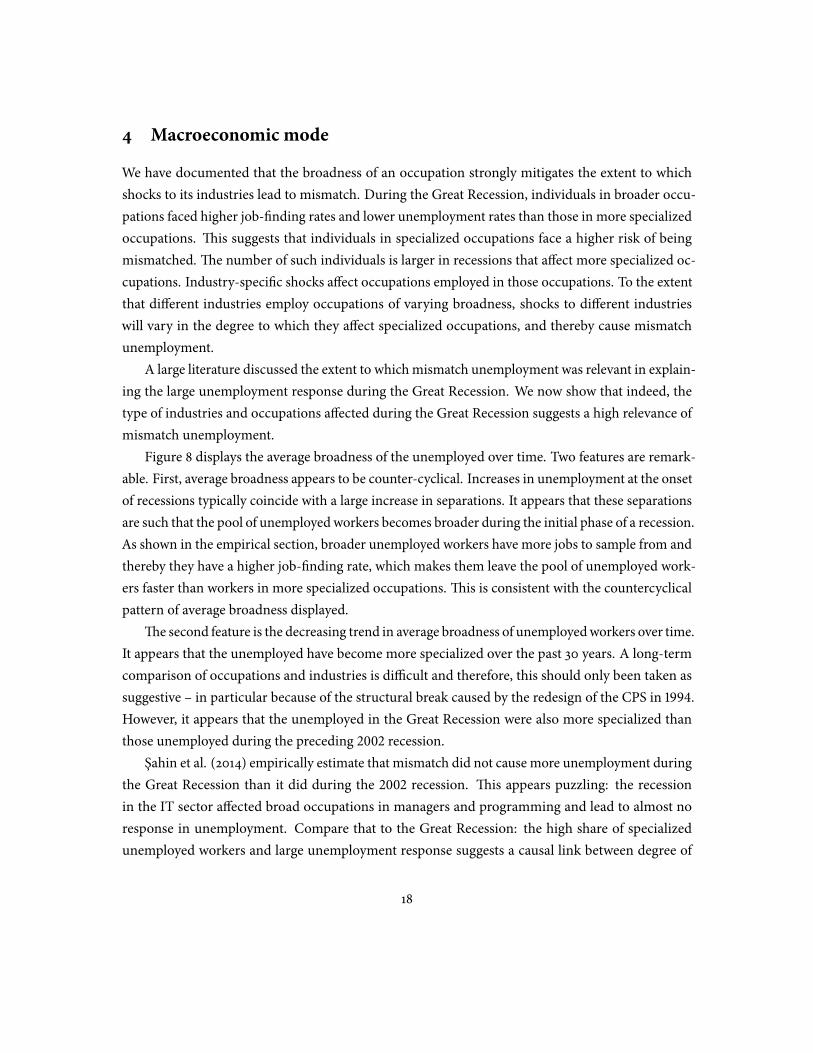
ing the large unemployment response during the Great Recession. We now show that indeed, thetype of industries and occupations aected during the Great Recession suggests a high relevance ofmismatch unemployment.Figure 8 displays the average broadness of the unemployed over time. Two features are remark-

able. First, average broadness appears to be counter-cyclical. Increases in unemployment at the onsetof recessions typically coincide with a large increase in separations. It appears that these separationsare such that the pool of unemployedworkers becomes broader during the initial phase of a recession.As shown in the empirical section, broader unemployed workers have more jobs to sample from andthereby they have a higher job-nding rate, which makes them leave the pool of unemployed work-ers faster than workers in more specialized occupations. is is consistent with the countercyclicalpattern of average broadness displayed.e second feature is the decreasing trend in average broadness of unemployedworkers over time.

It appears that the unemployed have become more specialized over the past 30 years. A long-termcomparison of occupations and industries is dicult and therefore, this should only been taken assuggestive – in particular because of the structural break caused by the redesign of the CPS in .However, it appears that the unemployed in the Great Recession were also more specialized thanthose unemployed during the preceding recession.Sahin et al. (2014) empirically estimate that mismatch did not cause more unemployment during

the Great Recession than it did during the recession. is appears puzzling: the recessionin the IT sector aected broad occupations in managers and programming and lead to almost noresponse in unemployment. Compare that to the Great Recession: the high share of specializedunemployed workers and large unemployment response suggests a causal link between degree of

18

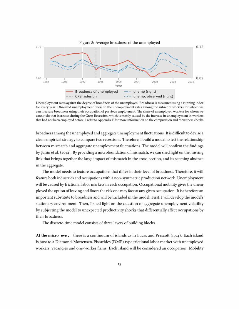
Figure 8: Average broadness of the unemployed

1984 1988 1992 1996 2000 2004 2008 2012 2016Year

0.68

0.78

0.02

0.12

Broadness of unemployedCPS redesign

unemp (right)unemp, observed (right)

Unemployment rates against the degree of broadness of the unemployed. Broadness is measured using a running indexfor every year. Observed unemployment refers to the unemployment rates among the subset of workers for whom wecan measure broadness using their occupation of previous employment. e share of unemployed workers for whom wecannot do that increases during the Great Recession, which is mostly caused by the increase in unemployment in workersthat had not been employed before. I refer to Appendix E for more information on the computation and robustness checks.

broadness among the unemployed and aggregate unemployment uctuations. It is dicult to devise aclean empirical strategy to compare two recessions. erefore, I build a model to test the relationshipbetween mismatch and aggregate unemployment uctuations. e model will conrm the ndingsby Sahin et al. (2014). By providing amicrofoundation ofmismatch, we can shed light on themissinglink that brings together the large impact of mismatch in the cross-section, and its seeming absencein the aggregate.e model needs to feature occupations that dier in their level of broadness. erefore, it will

feature both industries and occupations with a non-symmetric production network. Unemploymentwill be caused by frictional labor markets in each occupation. Occupational mobility gives the unem-ployed the option of leaving and oors the risk onemay face at any given occupation. It is therefore animportant substitute to broadness and will be included in the model. First, I will develop the model’sstationary environment. en, I shed light on the question of aggregate unemployment volatilityby subjecting the model to unexpected productivity shocks that dierentially aect occupations bytheir broadness.e discrete-time model consists of three layers of building blocks.

At the micro level, there is a continuum of islands as in Lucas and Prescott (1974). Each islandis host to a Diamond-Mortensen-Pissarides (DMP) type frictional labor market with unemployedworkers, vacancies and one-worker rms. Each island will be considered an occupation. Mobility

19

Figure 9: e input-output structure between occupations and industries

Industries

Occupations

narrowbroad

Final sector

Industries

Occupations

narrowbroad

Final sector

Intermediate Good

e production network of the economy. Notice that the two networks are isomorphic, as Section 4.3 shows.

across islands is frictional: the unemployed can change islands only aer incurring a xed cost thatcaptures loss of occupation-specic human capital and red tape. Additionally, the employed and theunemployed exit the labor force at the exogenous rate ζ . Newworkers enter the labor force at the samerate, decide which occupation to enter rst, and begin their careers as the unemployed. One-workerrms in each occupation produce a dierentiated intermediate good that is sold to industries.

At the meso-level, a continuum of islands buy the occupation-specic inputs, face idiosyncraticand persistent productivity shocks and produce dierentiated industry-specic goods. I assume aproduction network between occupations and industries that is not symmetric: occupations dierin the demand structure for their produced services.e model features two types of occupations. A measure γ of occupations is labelled “broad”:

they provide a service that is employed by a large number of industries. Ameasure −γ of occupationsis labelled “specialists” and provides a service that is only used by a single industry. is input-outputnetwork is illustrated in Figure (9). Because of their distinct demand structure, broad and specialistoccupations are dierentially aected by these shocks.

In the aggregate, the nal good is produced by aggregating the output from the continuum ofindustries. e model is stationary: individual industries and occupations are volatile, but we focusour attention to equilibria where aggregate variables such as total output and average unemploymentwill remain constant over time.I will now describe these building blocks in more detail.

20

4.1 Final sector

ere is a unit measure of industries that each produces intermediate output y(i). e nal sectorproduces aggregate output Y by integrating the output from the industries with elasticity θ. eenvironment is dynamic. For ease of exposition, I ignore time indices until they are necessary.

Y = [ ∫[,] y(i)θ−θ di]

θθ−

(5)

p(i) = (Yy(i)

)

θ

(6)

4.2 Specialized industries

Each industry i features a competitive equilibrium in which rms produce the intermediate outputy(i) at zero prot. Each specialist industry i is linked to a unique specialist occupation with thesame index. Firms in the linked occupation i provide intermediate output z(i) which is used byrms in industry i in the production of y(i). is is illustrated by (7), where A(i) is the industry-specic idiosyncratic productivity shock. Notice that the industry-level problem is static. Denotethe industry-specic and occupation-specic prices as p(i) and pz(i). Perfect competition impliesthat industry-specic prices are computed as input prices divided by productivity (8)

y(i) = A(i)z(i) (7)

p(i) = pz(i)A(i)

(8)

4.3 Broad industries

Firms in each broad industry i employ a CRS production function with elasticity of substitution θb.ey use labor services from occupations indexed o ∈ [, γ].

y(i) = A(i)x(i)

x(i) ≡ [Ax ∫[,γ] z(i , o)θb−θb do]

θbθb−

21

where as before, A(i) denotes industry-specic productivity. Ax is a constant productivity parameter,and z(i , o) denotes how much input of occupation o rms in industry i are using. Firms in broadindustries also face perfect competition. e rms’ problem is to optimize their input compositionfor a given vector of prices and a given level of output (9).

minz(i ,o)o ∫[,γ] pz(o)z(i , o)do (9)

s.t. y(i) = A(i) [ ∫[,γ] z(i , o)θb−θb do]

θbθb−

e appendix shows that optimal input composition is given by (10), where Px is the price indexassociated with producing x(i). e optimal input composition is identical across industries, as theyonly dier in their productivities. is dierence in productivities only aects their level of output,but not the composition of x(i).

z(i , o)x(i)

= (Px

pz(o))

θb,∀i , o (10)

Px = [Ax ∫[,γ] pz(o)−θb]

−θb

We use this result to solve for the equilibrium in the broad sectors as follows: we dene x to bethe total intermediate good available, produced using all occupation-level services as input:

x ≡ [Ax ∫[,γ] z(o)θb−θb do]

θbθb−

x = ∫[,γ] x(i)di (11)

e question remains as to how x is distributed across industries. e appendix answers thisquestion by using feasibility (11) and a rewritten rm’s problem to compute equilibrium x(i) shares(12). For each industry, its share of intermediate inputs relates to its idiosyncratic productivity A(i),an average productivity-index across broad industries Ab, as well as the elasticity of substitutionacross industries θ, as shown in (12).

22

x(i)x

= (A(i)Ab

)

θ−

(12)

Ab = [ ∫[,γ] A(i)θ−di]

θ−

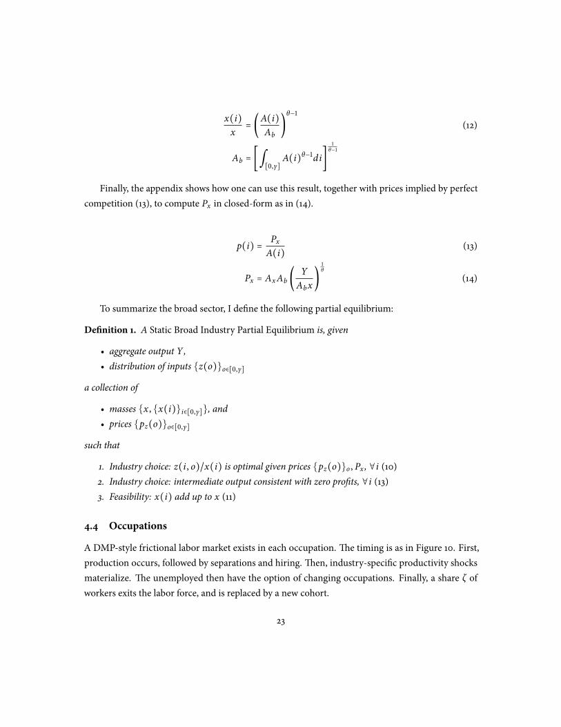
Finally, the appendix shows how one can use this result, together with prices implied by perfectcompetition (13), to compute Px in closed-form as in (14).

p(i) = PxA(i)

(13)

Px = AxAb (YAbx

)

θ

(14)

To summarize the broad sector, I dene the following partial equilibrium:

Denition 1. A Static Broad Industry Partial Equilibrium is, given

• aggregate output Y ,• distribution of inputs z(o)o∈[,γ]

a collection of

• masses x , x(i)i∈[,γ], and• prices pz(o)o∈[,γ]

such that

1. Industry choice: z(i , o)/x(i) is optimal given prices pz(o)o , Px , ∀i (10)2. Industry choice: intermediate output consistent with zero prots, ∀i (13)3. Feasibility: x(i) add up to x (11)

4.4 Occupations

A DMP-style frictional labor market exists in each occupation. e timing is as in Figure 10. First,production occurs, followed by separations and hiring. en, industry-specic productivity shocksmaterialize. e unemployed then have the option of changing occupations. Finally, a share ζ ofworkers exits the labor force, and is replaced by a new cohort.

23

Figure 10: Timing of events within each period

t

production, vacancies

hiring, separation

productivity shocks realize

mobility

labor force entry, exit

t + ∆

Figure 11: Dynamics within each occupation

M(m(Ω))

V (Ω)(−c)

J(Ω)(p(Ω) − w(Ω))

U(Ω)(b)

E(Ω)(w(Ω))

Exit(0)

Exit(0)

Uq(m(Ω))) f(m(Ω))

δ

δ + ζ ζ

ζU − k > U?

emain innovation compared to the canonical DMP setup is labor market mobility aer therealization of productivity shocks. Here, productivity shocks are not realized at the start of the period.is is slightly unconventional but simplies the notation when dening labor market adjustment:the denition of a period start will not aect any outcomes in the model.Figure 11 summarizes the dynamics within all occupations, both broad and specialized. As the

gure suggests, the fundamental structure of all occupations is the same. Broad and specializedoccupations dier in their price function p(Ω), as they face a dierent demand structure. erelevant state variable Ω diers across broad and specialized occupations – we will discuss thesedierences in detail.e purple boxes in the schematic are standard in the DMP environment: posting a vacancy

implies a ow cost of c, and the value function of vacancies is denoted as V . e unemployed’s valuefunctions are denoted asU , they receive b in each period. emarket tightness is denoted asm = v/u.e unemployed and the vacancies match according toM(m(Ω)). e resulting one-worker rmsproduce output at value p(Ω), of which the workers receives wage w(Ω). e value functions ofrms and workers are denoted as J and E. Matches separate at rate δ. When that happens, workersbecome unemployed and the rms simply exit.

24

e white boxes in that schematic are nonstandard. In each period, the unemployed have theoption of incurring xed cost k and changing their occupation. I assume that relocation is directedand workers have perfect information: if they decide to leave, workers will relocate to the occupationthat delivers the highest attainable utility U . We take U as given here, but will endogenize it later on.k summarizes loss of human capital and other barriers to occupational mobility.e second innovation is exogenous labor force exit. I assume labor force exit for a technical rea-

son: in its absence, multiple steady states may exist. At rate ζ > , the employed and the unemployedexit the labor force. Firms connected to exiting workers also exit the market.Next, I provide a more technical summary of the model. Note that the state vector Ω, all value

functions and policy functions dier across broad and specialized occupations and require subscriptj ∈ b, s. I now drop this subscript for clarity, but will add it when required.Denote the value of staying in an occupation as U stay(Ω). As they have to pay a xed cost k, we

can dene the value before the leaving stage as

U(Ω) = maxU stay(Ω),U − k

In each period, the unemployed either nd a job at rate f (m(Ω)), or stay unemployed and areallowed to change occupations again. Both employed and unemployed workers exit the labor forceat the exogenous rate ζ with the terminal value . is implies that the eective discount rate ρ is asum of both impatience and the exit rate: ρ = ρ + ζ .

U stay(Ω) = b∆ + e−ρ∆ [( − e− f (m(Ω))∆)E[E(Ω′

)] + e− f (Ω′)∆E[U(Ω)]] (15)

Vacancies match at rate q(m). e remaining value functions can be written as

E(Ω) = w(Ω)∆ + e−(ρ+ζ)∆E [e−δ∆E[E(Ω′)] + ( − e−δ∆)E[U(Ω′

)]] (16)

J(Ω) = [ps(Ω) −w(Ω)]∆ + e−(ρ+ζ+δ)∆E[J(Ω′)] (17)

V(Ω) = −c∆ + ( − e−q(m(Ω))∆) e−ρ∆E[J(Ω′

)] (18)

In equilibrium, market tightness is governed by free entry, (19), and wages are determined byNash bargaining with workers’ bargaining power β, (20).

25

V(Ω) = (19)

βJ(Ω) = ( − β) (E(Ω) −U(Ω)) (20)

Connecting occupations and industries Firms in broad and specialized occupations dier in theset of industries they provide their input for. is implies dierent demand structure and pricingfunctions for their output. is model is structured with simplifying the computation of these pric-ing functions in mind: we will now derive analytical solutions for the pricing functions of bothoccupation types. e logic will be the same: industry-level prices are given by the nal sector CESaggregator, given industry-level output. Industry-level output is a function of occupation-level out-put. Since all rms produce one unit of output, it is sucient to know occupation-level employmentto compute occupation-level output.For specialized occupations, this amounts to using (6), industry-level technology (7), and free-

entry, (8), to compute ps (21). ps is a composite of a, and a bracketed term. e bracketed termcomputes the price of industry-level output, combining total occupation-level input ( − u)ℓ andindustry-level productivity a. e outer a translates occupation-level output into industry-leveloutput and ensures that occupation-level rms gain all the revenues from selling multiple unitswhenever their connected industry is more productive.is pricing function ps determines the state vector: u and ℓ together yield the number of one-

workerrms. For each specializedoccupation, the productivity of the connected industry a is relevantto compute industry-level output and prices, and hence appears in the state vector. Aggregate outputY is constant, and hence does not characterize the state space. at is, the specialist occupation’sstate vector can be written as Ωs = a, u, ℓ.

ps(a, u, ℓ) = a (Y

a( − u)ℓ)

θ

(21)

pb(u, ℓ) = (x

( − u)ℓ)

θb⋅ Px (22)

We apply a similar logic for the price of output from broad occupations, pb. Using the appropriateequations from the industry side together with feasibility, we obtain pb (22). is price is composedof two products: the rst bracketed term denotes the relative importance of any particular occupation

26

in producing x. e second term Px denotes the value of each unit of output x. Broad occupationsare perfectly insured against industry shocks since they can sell to any industry i ∈ [, γ]. is iswhy no productivity-related variable a is required to compute pb: the relevant state vector for broadoccupations is Ωb = u, ℓ.

Laws of motion It remains to describe the transitions for Ωb and Ωs. I will denote by gx; j the lawof motion for dimension x ∈ a, u, ℓ and occupation type j ∈ b, s. We begin with specializedoccupations. For now, we will take the law of motion for the labor force gl ;s(a′, a, u, ℓ) as given.Productivity a follows an AR(1) process, and the law of motion for the unemployment rate has to becorrected for changes due to migration:

gu;s(a, u, ℓ, ℓ′) = − e−ζ∆( − u(a, u, ℓ))ℓℓ′

(23)

u(a, u, ℓ) = ( − e−δ∆)( − u) + e− f (m(a,u,ℓ))∆u

where u(Ω) denotes the unemployment rate post separations and matching, but prior to relocation.Note that without relocation (ζ = and ℓ′ = ℓ), we recover gu;s = u.Laws of motion for broad occupations are similar. e main noticeable dierence is the lack of

a as a state variable.

ub(u, ℓ) = ( − e−δ∆)( − u) + e− f (mb(u,ℓ))∆u

gu;b(u, ℓ, ℓ′) = − e−ζ∆( − ub(u, ℓ))ℓℓ′

(24)

We can summarize each type of occupation by dening a partial equilibrium.

Denition 2. A Stationary Recursive Specialist Occupation Partial Equilibrium takes as given

• A price function ps(Ωs)

• A law of motion for labor gℓ;s(Ωs)

• A leaving utility U

and contains

• A set of value functions Js(Ωs), Es(Ωs),U stays (Ωs),Us(Ωs),• Wages ws(Ωs)

27

• Law of motion for u gu;s(Ωs , ℓ′),• Market tightness ms(Ωs)

such that

1. Given gu;s ,w,U ,Y : Js , Es ,U stays ,Us satisfy (15)-(17)2. Given Js , Es ,U stays : wages satisfy Nash bargaining (20)3. Given Js: m satises free-entry (19)4. Law of motion gu;s is consistent with m (24)

Denition 3. A Recursive Broad Occupation Partial Equilibrium is, taken as given

• A price function pb(Ωb)

• A law of motion for labor gℓ;b(Ωb)

• A leaving utility U

and contains

• A set of value functions Jb(Ωb), Eb(Ωb),Ustayb (Ωb),Ub(Ω),

• Wages wb(Ωb)

• Law of motion for u gu;b(Ωb , ℓ′),• Market tightness mb(Ωb)

such that

1. Given gu;b ,w,U ,Y : Jb , Eb ,Ustayb ,Ub satisfy (15)-(17)

2. Given Jb , Eb ,Ustayb : wages satisfy Nash bargaining (20)

3. Given Jb: m satises free-entry (19)4. Law of motion gu;s is consistent with m (25)

4.5 Mobility

So far, labor force ows across occupations have been taken as exogenous. Here I describe the laborforce ows that will be consistent with individual-level decisions.e unemployed can incur a movement cost k and move to any occupation of their liking. We

presume that if they move, they will go to the occupation that will deliver the highest expected utilityto an unemployed worker. is highest utility in each sector is denoted as Ub and Us.

28

Ub = max(u,ℓ)∶gb(u,ℓ)>

Ub(u, ℓ)

U s = max(a,u,ℓ)∶gs(a,u,ℓ)>

Us(a, u, ℓ)

where gb and gs denote the density of broad occupations over the (u, ℓ) space, and specialistoccupations over the (a, u, ℓ) space.Asmentionedbefore, themobility cost is independent of the type (broad/specialist) of originating

and destination occupation. erefore, the relevant variable for the optimization problem is the bestattainable utility of any of those, denoted U . e present-discounted value of moving net of themigration cost k will be denoted U .

U = maxUb , Us

U = U − k

It is optimal for the unemployed to leave whenever their next period’s value Ub(Ω′b) or Us(Ω′

s)

is below U . All unemployed workers have this option, and will use it whenever their utility Ub(u, ℓ)or Us(a, u, ℓ) < U . In what follows, I will describe the law of motion for the labor force in the broadoccupations (25).To understand mobility, denote by U ′(gℓ) next-period utility as a function of mobility at the

end of this period. ere are four cases to distinguish. In case (i) U ′() ∈ (U ,U).. If withoutmobility, next period’s utility is strictly between the boundaries, there is no incentive for workers toleave. Moreover, as occupation does not belong to the set of “best occupations for the unemployedto enter”, no worker will enter. In case (ii) U ′() ≥ U : next period’s utility would be at or above U .In equilibrium, U has to be the highest attainable utility value: we will observe positive mobility intothe occupation. However, positive mobility is only an equilibrium outcome if U ′(gℓ) ≥ U . us, weknow that mobility will be such that U ′(gℓ) = U . Next, we have to deal with U ′() ≤ U . Wheneverthat is the case, unemployed workers will leave the occupation. e measure leaving is such thateither (iii) all unemployed workers have le, but next-period’s utility remains below the threshold, or(iv) the utility has moved to the threshold U – whatever requires fewer mobility. e law of motionfor the specialist occupations’ labor force (26) follows the same spirit.

29

g ℓ;b(u,ℓ)

=

⎧ ⎪ ⎪ ⎪ ⎪ ⎪ ⎪ ⎪ ⎪ ⎪ ⎪ ⎨ ⎪ ⎪ ⎪ ⎪ ⎪ ⎪ ⎪ ⎪ ⎪ ⎪ ⎩

e−ζ∆ℓ

ifUb(g u

;b(u,ℓ,e−

ζ∆ℓ),e−ζ∆ℓ)

∈(U,U

)

x∶Ub(g u

;b(u,ℓ,ℓ′=x),x

)=U

ifUb(g u

;b(u,ℓ,e−

ζ∆ℓ),e−ζ∆ℓ)

≥U

(−

u b(u,ℓ)

)e−

ζ∆ℓ

ifUb(g u

;b(u,ℓ,e−

ζ∆ℓ),e−ζ∆ℓ)

<U

x∶Ub(g u

;b(u,ℓ,ℓ′=x),x

)=U

otherwise

(25)

g ℓ;s(a′,a,u,ℓ)=

⎧ ⎪ ⎪ ⎪ ⎪ ⎪ ⎪ ⎪ ⎪ ⎪ ⎪ ⎨ ⎪ ⎪ ⎪ ⎪ ⎪ ⎪ ⎪ ⎪ ⎪ ⎪ ⎩

e−ζ∆ℓ

U(a′,g

u(a,u,ℓ,e−

ζ∆ℓ),e−ζ∆ℓ)

∈(U,U

)

x∶U(a′,g

u(a,u,ℓ,ℓ′=x),ℓ′=x)

=U

U(a′,g

u(a,u,e−

ζ∆ℓ,e−

ζ∆ℓ),ℓ)≥U

(−

u(a,u,ℓ)

)e−

ζ∆ℓ

U(a′,,e−ζ∆(−

u(a,u,ℓ)

)ℓ)

≤U

x∶U(a′,g

u(a,u,ℓ,ℓ′=x),ℓ′=x)

=U

elseifU(a′,g

u(a,u,e−

ζ∆ℓ),,e−

ζ∆ℓ)

≤U

(26)

30

4.6 General equilibrium

So far, we have described the building blocks of the model in isolation. To close the model, twomargins need to be addressed. First, Y is being taken as exogenous by all agents in the economy,but must be consistent with industry-level output. Second, the amount of inputs used by industries∫ z(i , o)di has to be consistent with the employment level at each occupation o. ird, the distribu-tion and ows of labor across occupations have to be consistent with the (constant) aggregate laborforce.

4.7 Connection between industries and occupations

Industries are lined up on the unit interval. Industries i > γ are specialist industries. Each industryhas a productivity stateA(i). It is linked to a specialist occupationwith state (a, u, ℓ), where a = A(i),and (u, ℓ) are drawn from the stationary distribution Gs(a, u, ℓ):

A(i) ∼ logNormal(s.t. stationary AR (1)) ∀i ∈ [, ] (27)

(u(i), ℓ(i)) ∼ Gs(a, u, ℓ∣a = a(i)) ∀i ∈ (γ, ] (28)

Industries i ≤ γ are broad industries. ey have productivity states A(i), but no (u, ℓ) state,since they are not linked to any particular occupation.We have the following feasibility constraint:

z(o) = ( − u(o))ℓ(o) ,∀o ∈ [, ] (29)

Prices for broad and narrow occupations come from the demand structure of the correspondingindustries:

pb(u, ℓ) = (x

ℓ( − u))

θbPx (30)

ps(a, u, ℓ) = a (Y

a( − u)ℓ)

θ

(31)

Feasibility in terms of labor is stated as follows:

31

L = γ ∫U×L ℓdGb(u, ℓ) + ( − γ) ∫A×U×L ℓdGs(a, u, ℓ)

L = Lb + ( − γ) ∫A×U×L ℓdGs(a, u, ℓ) (32)

where L is a parameter.

Denition 4. A General Equilibrium is a collection of

1. Aggregate output Y2. Specialist industry states A(i), u(i), ℓ(i)i∈(γ,]3. Broad industry states A(i)i∈[,γ]4. Occupation-level distributions Gb(u, ℓ),Gs(a, u, ℓ)5. Occupation-level output z(o)o∈[,γ]6. Leaving threshold U7. Laws of motion for labor gℓ;s(a, a′, u, ℓ), gℓ;b(u, ℓ)8. Prices of occupation-specic output ps(a, u, ℓ), pb(u, ℓ)9. All previous variables (value-functions, masses, prices...)

such that

1. Y is consistent with industry output (5)2. z(i) is consistent with occupation-level output (29)3. Specialist industry states consistent with specialist occupation distribution (28)4. U is consistent with Gb ,Gs

5. Prices are consistent with industry-level demand and feasibility (30)-(31)6. Laws of motion for labor are consistent with U ,U (25)-(26)7. Gb ,Gs are consistent with the productivity process and gℓ;s , gℓ;b , gu;s , gu;b8. ∀i ∈ (γ, ]: given A(i), z(i): p(i) solves specialist industry prices (8)9. ∀i ∈ (γ, ]: given ps(a, u, ℓ), gℓ;s ,U: Js , Es ,Us ,w , gu;s ,ms solve Stationary Recursive Spe-cialist Occupation PE

10. ∀i ∈ [, γ]: given Y , z(o)i∈[,γ]: x , x(i), pz solve Broad Industry PE11. Given Lb , pb(u, ℓ),U ,U: Jb , Eb ,Ub ,m, u, gu;b solve Recursive Broad Occupation PE12. Feasibility w.r.t L (32)

32

Table 3: Parameters of the model

Parameter Value Description Source

Generalρ 0.001 Discount rate∆ 0.333 Length of periodIndustriesσ 0.050 Productivity stdρA 0.800 Productivity autocorrθ 4.500 Elasticity, Final sectorNetworkAx 4.322 Productivity (x) Labor force distributionγ 0.500 Measure of broad occupations Illustrationθ 0.500 Elasticity, broad industries High complementarityOccupationsA 1.355 Matching productivity Literatureα 0.510 Matching elasticity Literaturec 0.127 Vacancy posting cost Average unemployment rateb 0.955 Home production HM (2008)β 0.052 Bargaining Power: Worker HM (2008)δ 0.100 Monthly separation rate Shimer (2005)ζ 0.006 Labor force entry/exit Average working yearsk 0.103 Moving cost

All rates in quarterly units.

4.8 Parameter selection

e general strategy behind parameter selection is to make the potential impact of broadness as largeas possible, so as to give this exercise the spirit of a benchmark. For other parameters, I will eitherselect values that expose the mechanism more clearly or are in line with the literature.e unit of time is a quarter. To prevent issues from time aggregation, the period length is a

month. Here, I trade o precision and computational complexity.In this paper, I study dierential responses between specialist and broad occupations. In the data,

broad occupations and industries dier in other dimensions that have little to dowith thismechanism.For the sake of exposing this particular mechanism, I do not recalibrate broad occupations andindustries to dierent productivity processes or labor market structures. While the discount rateappears small, together with the labor force exit rate, they add up to an eective annual discount rateof ..

33

Industries I assume that volatility and persistence of industry-specic productivity processes are ofsimilarmagnitude of those typicallymeasured for aggregate productivity. Higher values here increasethe insurance provided by broadness. I normalize the average broad and specialist innovations to bezero. Industry-specic goods are substitutes, which implies that a positive productivity shock at theindustry level yields higher equilibrium employment in linked occupations. By choosing high valuesfor σ and θ, I increase the role for broadness: large productivity shocks and highly substitutableindustry-level outputs will imply that labor demand is highly elastic with respect to productivityshocks. In this type of environment, the dierence in volatility of unemployment between broad andspecialized occupations will be higher.

Network I have empirically measured the average broadness of the economy to be .. However,to more clearly expose underlying mechanisms, I will set γ = ., as this will ease the comparisonbetween shocks to broad and specialized industries. e main results from the aggregate exercisesare independent of γ, and I will emphasize whenever that is not the case. e labor-force weightedaverage broadness of the economy is similar to the average occupation-level broadness, and thereforeI calibrate Ax to yield an average labor force share of γ in broad occupations. ere is little evidenceon the within-sector substitutability of dierent occupations. Finally, θ has been understudied in theempirical literature. Here, all broad occupations are identical, and therefore aggregate uctuationswill not induce any substitution across occupations. Hence, θ only plays a role in relative productivitybetween broad and specialized occupations, something that is already calibrated using Ax . In anycase, I have used the rise and fall of construction-specic demand together with relative weak outsideoptions for blue-collar workers in the construction sector to estimate an elasticity of substitutionaround . between blue-collared and white-collared workers in the construction sector. Recogniz-ing that the chosen split and sector are at the lower end of the distribution for θ, I choose θ = .. Asemphasized before, this particular parameter does not aect the results.

Occupations Shimer (2007) makes the point that perfectly competitive local labor markets candisplay an aggregate behavior similar to the typically calibrated matching function. at is, thereis no bijection between aggregate labor ows and required local labor market matching functions.Moreover, vacancy data is quite noisy and a precise estimation of matching parameters at the occu-pation level appears infeasible. erefore, there is no clear and robust empirical guidance to set uplabor-market-level matching parameters. α is set to a median value in the domain between and, in line with Petrongolo and Pissarides (2001). As explained in Shimer (2005), the level of markettightnessm is meaningless. e productivity of the matching function A controls this level and there-

34

fore I simply set A to the value in Shimer (2005). I calibrate c to match an average unemploymentrate of u = ..ere are several ways of creating high unemployment uctuations in this environment. One

can select a wage process that is more persistent than what is implied by Nash bargaining, forceproductivity to be very volatile, or calibrate the rm’s share of the surplus to be small and volatile. Forease of implementation, I here choose to do the latter and follow Hagedorn and Manovskii (2008)in calibrating home production and bargaining power. While this does aect the absolute responsesof unemployment rates to a productivity shock, relative unemployment rates across occupations willnot be aected.Finally, k will govern the rate at which workers respond to shocks by changing occupations.

Unfortunately, there is no causal evidence of the link between occupation-specic shocks and exitrates. Moreover, even the unconditional rate at which the unemployed change occupations is notwell documented. is is because occupation data is measured with noise. Since occupation changesare measured as dierences in individual-specic occupation tags, measurement error attributes toan upward bias in estimated occupational transition rates. e CPS introduced dependent coding in1995 to address this issue. However, unemployed agents’ occupation tags are still measured withoutdependent coding. I summarize this issue in Appendix D and argue that, in practice, observedoccupational mobility is not a good target for k. To calibrate k, I simulate an economy in whichmobility is impossible. I observe the uctuations in the unemployed’s value function, and computethe corresponding th and th percentiles. k is set to match the dierence in these percentilevalues. Notice that the resulting k is small: the costs of changing occupations are around one tenth ofa worker’s average quarterly wage. I will emphasize results that depend on the resulting calibrationfor k.

4.9 Steady state

is model nests occupational directed search with random search in each occupation. Moreover,each occupation has decreasing returns to scale. ese components, together with the exogenouslabor force exit rate, ensure that the steady state is unique. It is useful to analyze the steady state togain some familiarity with the environment before moving on to the question that this model wasdesigned to address.Table 4 summarizes some aggregate statistics of the steady state. As most of the labor force

is in broad occupations and industries are substitutes, the production of total output draws morefrom broad industries, which in equilibrium sell their intermediate goods at lower prices. However,

35

Table 4: Key statistics of the steady state

Moment Value Description

IndustriesY 0.9619 Total outputyb 0.3980 Total output, broad indys 0.3887 Total output, narrow indPb 1.2166 Price index, broadPs 1.2231 Price index, specialistOccupationsvb 0.3139 Vacancies, broadE[vs] 0.4249 Vacancies, specialistub 0.0492 Unemp, broadEℓ[us] 0.0564 Unemp, narrow occ (weighted average)std[us] 0.0216 Unemp, narrow occ (weighted std)E[wb] 1.0000 Wage, broad occE[ws] 1.0020 Wage, narrow occ (average)Lb 0.5050 Measure broad labor

this large dierence in prices is not visible in wages: because of free entry of rms, dierences insector-level prices are dominated by dierential entry costs, as there are more vacancies in specialistoccupations.

4.9.1 Mobility and compensating dierentials

We begin our steady state analysis by analyzing the behavior of individuals within a single givenoccupation. Figure 12 plots the value functions for unemployed workers in specialized occupationsover the three state variables. All three state variables impact the value of occupation-level rms.As the unemployed expect to eventually become employed, a change in the value of rms will bere ected in wage changes, and thereby aect the value of the unemployed.Higher productivity will imply a higher total production of the industry-level good, which lowers

industry prices and hence occupation-level prices. However, each rm in each industry is able toproduce more output, which overcomes the price eect and implies that the occupation-specicoutput yields a higher price when productivity increases. When the labor force increases, themeasureof occupation-specic rms increases and the evaluation of occupation-specic goods decreases, thusreducing the price of the occupation-level good. e less intuitive dimension is the unemploymentrate: a higher unemployment rate increases the value of the unemployed. is is because we are

36

Figure 12: Value function of the unemployed

−0.1 0.0

log productivity

129.86

129.88

129.90

129.92 U(a, u, l)U lowU high

0.0 0.1 0.2 0.3

unemployment rate1.0 1.1 1.2 1.3

labor forceValues at constant dimensions: a=0.03, u=0.07, l=0.99

holding all other dimensions constant. In this class of models, free entry pins down a rate of markettightness: a higher unemployment rate will, ceteris paribus, simply mean a higher vacancy rate, andwill not aect the job-nding rate. Additionally, a higher unemployment rate implies that a smallershare of workers are employed, which leads to a higher price of the occupation-level good.e key take-away from the value functions is that individuals typically want to enter into an

occupation that has high productivity and a low labor force, and leave those with high labor forceand low productivity. We can see this more clearly when looking at the path of an occupation overtime. Figure 13 plots the dynamics of a specialized simulated occupation. e rst three panelsdisplay the evolution of the state vector Ωs = a, u, ℓ. a is exogenously drawn from the industry’sproductivity sequence, while u and ℓ are equilibrium outcomes. e fourth panel displays U(Ωs),which is in equilibrium bound between U and U . Episodes where Us is at its entry and exit valuesare highlighted in green and purple. Whenever a positive productivity shock would push Us aboveU , ℓ increases to prevent that from happening. Notice that these migrants start unemployed, andwe can see a spike in u at those periods. Labor markets are calibrated to capture the uidity of theUS labor markets. In good times, these additional unemployed workers nd a job very quickly, andthese spikes in u vanish quickly: mobility does not contribute largely to measured unemployment uctuations.Whenever the occupation is not at the upper boundary, we have nomobility into that occupation.

Exogenous labor force exit will slowly reduce the labor force present in the occupation. is acts as astabilizing factor: we observe much more directed mobility into an occupation than out of it. In thisparticular simulation, there is only one episode where active exit out of an occupation was necessary.at episode is highlighted in purple. As unemployed individuals are those that exit the occupation,

37

Figure 13: Dynamics of a simulated specialized occupation

1.0

1.1a

0.05

0.10

u

1.0

1.1`

0 5 10 15 20 25 30

t (quarters)

U

U

U(a, u, `)

Dynamics of a simulated specialized occupation. First three panels draw the evolution of the state vector a, u, ℓ, andthe fourth panel depicts the evolution of the value function.

we observe a sharp decline in both labor force and unemployment rate.Next, we analyze the stationary distribution that is implied by the dynamics of each occupation.

Figure 14 displays the cross-sectional distribution of labor markets. e blue and red lines denotethe lower and upper boundary of the labor force for any given unemployment rate and productivity.Notice that these boundaries increase in both productivity and unemployment rates, as the valuefunctions also increase in a and u. Occupations move in this state space for three reasons. First,productivity shocks will shi occupations across these panels. Second, an occupation’s (u, ℓ) adjustsif it nds itself outside of (ℓ, ℓ) at the new productivity state a′. ird, unemployment rates changeanytime they are not equal to the stationary unemployment rate implied by the current job-ndingrate. Fourth, an exogenous labor force exit will lead to a slow depreciation of labor, until occupationsare pushed towards ℓ.Notice that many occupations with the lowest productivity state have a higher unemployment

rate than occupations with the highest productivity state. is is because unemployment rates are notonly a function of the job-nding rate, but also of mobility: occupations with high productivity stateswill receive a lot of occupation switchers, who start unemployed, thereby increasing their unemploy-ment rate. On the other hand, the unemployed leave low productivity occupations, decreasing theirunemployment rate.

38

Figure 14: Mobility

0.0 0.1 0.2

u

0.75

1.00

1.25

`

a = −0.16

0.0 0.1 0.2

u

a = −0.03

0.0 0.1 0.2

u

a = 0.03

0.0 0.1 0.2

u

a = 0.16

`(a, u) `(a, u) g(a, u, `)

e distribution of specialized labor markets across productivity, unemployment rates and labor force, for four selectedproductivity states. Circle size is proportional to mass.

Figure 15: Key labor market variables in specialized and broad occupations

130.95 131.00 131.05

U

0.1 0.2 0.3

J

0.00 0.05 0.10 0.15

u

1.00 1.05

w

Red: distribution of variable across specialized occupations, with red line denoting mean. Blue: (degenerate) distributionof variable across broad occupations.

39

4.9.2 Compensating dierentials and wage proles

Nowwe highlight wage formation in this model. Figure 15 displays a few labor market characteristicsfor both broad and specialized occupations. e rst panel displays the distribution of the utilitiesof the unemployed in specialized occupations against those in broad occupations. e distributionof labor markets in broad occupations is degenerate on (u, ℓ), which is why Us collapses on a singlevalue, indicated by the blue line. Without exogenous mobility, any Ub ∈ [U ,U] would be consistentwith a steady state. As we have chosen ζ > , Ub = U is the unique equilibrium: for any Us < U wehave positive exit but no entry, inconsistent with the dened steady state.is will mean that averageUb is higher than averageUs in this economy in any equilibriumwith

non-zero k. e strict relationship between U and J implies that also Jb > E[Js], as can be seen inthe second panel. From the free-entry condition, this will imply a strictly higher market tightness inbroad occupations, and thus a higher job-nding rate in broad occupations. As the third panel shows,this higher job-nding rate leads to a lower unemployment rate on average in broad occupations.Wages are on average equal in the two economies: there is no compensating dierential for choosingthe more risky specialized occupations. is is because agents are risk-neutral.However, there are still some interesting wage dynamics going on in specialized occupations. To

see these, Figure 16 again considers the simulated specialized occupation that we have seen earlier.Now, instead of plotting the evolution of utilities Us, we plot the evolution of wages ws. Wheneverthere is mobility into the occupation, wages in the occupation are higher than average. Wages thenrevert back to average, and eventually are even lower than those in broad occupations. is is becauserelocation frictions prevent households from moving to broad occupations as soon the wage rate intheir current occupation is dominated by that of broad occupations. Eventually, when the state ofthe occupation deteriorates too much, individuals leave.At the rm level, ecient contracts under one-sided commitment oen imply that rms hire

workers at a low wage rate, but promise them a steep wage prole. is reduces turnover as workersstay to receive the higher promised future wages. In this environment, workers are already “stuck”in their labor market. To be enticed to enter an occupation that is eventually deteriorating, workersreceive a starting wage that is higher than that in broad occupations.We conclude that in this particular framework with risk-neutral agents, workers need not be

compensated for the additional riskiness of specialized occupations. However, they are being compen-sated for the expected deterioration of their labor market by receiving a higher wage when entering.

40

Figure 16: Evolution of wages in specialized occupations

1.0

1.1a

0.05

0.10

u

1.0

1.1`

0 5 10 15 20 25 30

t (quarters)

wb

w(a, u, `)

Dynamics of a simulated specialized occupation. First three panels draw the evolution of the state vector a, u, ℓ, andthe fourth panel depicts the evolution of wages.

5 Aggregate shock

Having set up the machinery, we can now turn to the eects from aggregate shocks. Before turningto the main results, I will summarize two additional experiments that I perform in the appendix, tohelp us understand the model better.In the rst exercise, I study a recession in which all industries are aected. Our intuition tells us

that broadness does not provide insurance against shocks that are perfectly correlated across indus-tries, and we would expect both types of occupations faring similarly in such a recession. AppendixF.1 shows that this is not the case: broad occupations are actually hit worse by aggregate shocks. Istudy this phenomenon in detail in the appendix. In short, the aggregate productivity shock interactswith the industry-specic productivity process. A negative productivity shock reduces the disper-sion of eective productivities across industries. All value functions are concave in productivity andhence benet from the relative compression. is eect is not present in broad occupations, whichexplains these qualitative ndings.Second, I study a recession in which both broad and specialized industries are aected in Ap-

pendix F.2. Qualitatively, this targets a period like that Great Recession, in which industries with oc-cupations of varying broadness were aected. In this exercise, I compare the response of job-ndingrates and unemployment rates across broad and specialized occupations, and can qualitatively re-produce the empirical ndings: In the same recession, broader occupations’ job-nding rates andunemployment rates were less responsive than those of the specialized occupations.Now, we turn our attention back to dierent types of recessions: ose that generate mismatch

41

because they aect specialized occupations. We contrast them against recessions that aect broad oc-cupations and hence generate less mismatch. We will see that the intuition from the cross-sectionalresults in the empirical section is misleading when estimating aggregate eects of mismatch: Re-cessions in more specialized occupations do lead to larger output losses, but not to larger or morepersistent unemployment responses.

A(i , t) =⎧⎪⎪⎪⎨⎪⎪⎪⎩

A(t) + A(i , t) if i ∈ I

A(i , t) else(33)

A(i , t) = ϕA(i , t − ) + єt

A(t) =⎧⎪⎪⎪⎨⎪⎪⎪⎩

µ if t ≤ T

else

Equation (33) describes the productivity process. A common aggregate component A(t) willaect the productivity of a subset of industries that belong to the set I . For those industries, theireective productivity sequence is the product of their idiosyncratic productivity A(i , t) and A(t).e remaining industries are not aected by the aggregate component. is aggregate component hasconstant value µ, and switches back to zero aer T quarters. In the following illustrative simulation,I set T to quarters. e productivity shock has size µ = −., and the size of I is .: % ofindustries are aected by the recession.is recession is unexpected by the agents. As soon as the initial shock hits, all agents have perfect

foresight about the remaining evolution of the process. is type of zero-probability aggregate shocksare oen referred to as “MIT shocks”.3

is experiment is comparing recessions that are aecting either broad or specialized occupations.ese recessions are identical in all but the type of industries that are aected. In one recession, the% of industries that are aected all have i < γ: only industries employing broad occupations areaected, and I refer to that recession as a “broad recession”. e other recession draws the measure. of industries among those with i > γ, and I call that recession a “narrow recession”.e top panel in gure 17 compares the evolution of the prices of occupation-specic goods across

both recessions. I contrast the value of broad goods in broad recessions against that of specializedgoods in specialized recessions. As established earlier, workers in broader occupations are insured

3Studying the economy’s deterministic response to shocks that are ex-ante unexpected is useful to understand itsresponse to recurring aggregate shocks, see Boppart, Krusell, and Mitman (2018)

42

Figure 17: Cross-sectional responses

0 2 4 6 8 10 12 14

0.98

1.00

pb(t), Broad shockps(t), Narrow shock

0 2 4 6 8 10 12 14

t (quarters)

2.0

2.5

3.0fb(t), Broad shockfs(t), Narrow shock

43

against industry-specic recessions as they can sell their good to unaected sectors. is insurancemanifests itself in a lower sensitivity of the price of the occupation-level good. e bottom panel plotsthe evolution of job-nding rates. e consequence of the price evolution is that the job-nding ratesof the unemployed in broad occupations are less responsive than that of specialized occupations.ese are the implications of the direct eect. ey qualitatively track what we measured in the

empirical section. However, we have to take into account the size of the populations aected by eachshock. e rst panel in Figure 18 compares the relative labor forces that are directly aected bythe shock in each type of recession: shocks in specialized industries directly aect the specializedoccupations that are connected. As a measure . of industries are shocked in each scenario, and thelabor force has been calibrated to be equally distributed among broad and specialized occupations,a measure . of workers is aected in the specialized recession. In contrast to that, the recessionin measure . of broad industries aects all workers in broad industries. In the model, this isbecause the reduction of occupation-level prices aects both rms that had been selling to the aectedindustries, and those that had been selling to industries which are not aected.In the real world, this important general equilibrium eect is more intuitive: engineers in con-

struction are insured against construction-sector shocks as they can move to other unaected indus-tries. However, by moving to other industries, they will aect workers that were previously alreadyactive in those industries. Broadness insures individuals against industry-specic shocks, but theoccupation as a whole has to take a hit.e second panel in Figure 18 addresses the question of mobility by comparing the relative

changes in the labor forces. In this model, moving entails a xed cost. erefore, individuals thatincur larger losses are more likely to change occupations. Workers in specialized occupations arenot insured against the shock: ey fare worse in the recession and respond more by changingoccupations. Workers that change occupations always target the best available labor market andtherefore dampen the impact of the aggregate productivity shock on the unemployment rate.e response of the aggregate unemployment rate is a composite of all these eects: how hard

are workers hit in the cross-section, how many of them are directly aected by either recession, andto what extent do they respond by changing occupation. Figure 19 compares the aggregate unem-ployment responses of the whole economy in both types of recessions. e aggregate unemploymentrate response is roughly similar in both types of recessions. e reason for the unemployment ratesbeing similar is the aforementioned general equilibrium eect: broadness insures the individual,not the whole occupation. us, a shock to specialized occupations aects few workers a lot, whilea shock to broad occupations aects many workers a little bit. Which type of recession leads to alarger unemployment response is model-specic. In this model, the important nonlinearity is the

44

Figure 18: Comparison compositions

0 2 4 6 8 10 12 14

0.2

0.3

0.4

0.5Lb(t), Broad shockLs(t), specialist shock

0 2 4 6 8 10 12 14

t (quarters)

0.980

0.985

0.990

0.995

1.000Lb(t), Broad shockLs(t), Narrow shock

Figure 19: Aggregate unemployment response

0 2 4 6 8 10 12 14

t (quarters)

0.052

0.054

u(t), Broad shocku(t), Narrow shock

45

Figure 20: Aggregate output response

0 2 4 6 8 10 12 14

t (quarters)

0.985

0.990

0.995

1.000 Broad shockNarrow shock

aforementioned occupation-switching. A shock to specialized occupations leads to larger relocationof labor. ese relocating workers move to labor markets with higher job-nding rates and therebyimprove the aggregate unemployment rate.is does not imply that a shock to broad occupations leads to a larger welfare drop. Here, the

appropriate welfare measure is aggregate consumption. e aggregate consumption is computedby subtracting the vacancy costs and the mobility costs from the aggregate output. e vacancycosts are comparable in both recessions, and the mobility costs are larger in the specialized recession.erefore, it is sucient to show that the output losses are larger in the specialized recession than inthe broad recession (Figure 20), to conclude that the shock to specialized industries leads to largerwelfare losses. Why are the output losses larger in a specialized recession? In the broad recession,rms in the broad occupations sell their output exibly to unaected industries. Firms in specializedoccupations do not have this option when their industries are aected in a specialized recession.ey continue to sell their output to the industries aected by the productivity shock. erefore, ashock to specialized industries leads to a larger misallocation of labor and larger output losses.

6 Conclusion

Understanding the determinants of unemployment is key in providing solid policy advice. ispaper connects the phenomenon of mismatch unemployment to two key outcomes: heterogeneousunemployment risk in the cross-section, and unemployment uctuations in the aggregate. I do soby modeling mismatch as a result of adjustment frictions across occupations and industries. ekey variation - dierences in broadness across occupations - is an important determinant of unem-

46

ployment risk in the cross-section. For policy makers, this is a concept that can be readily appliedto estimate exposure of occupations to unemployment uctuations and guide labor market poli-cies. e externalities of occupational mobility leave room for welfare gains of policy improvements.For example, occupational retraining could be targeted at more specialized occupations to provideinsurance to workers that are particularly aected by a recession.ese strong cross-sectional results are contrasted by the missing eect of mismatch in the ag-

gregate. In the model, recessions that cause more mismatch do not lead to larger unemployment uctuations. is is because the direct eect is confronted by a general equilibrium eect cased byworkers in broad occupations that switch industry and thereby spread the impact of the recessionontomore productmarkets. ese two eects are of similar order ofmagnitude. e exact qualitativedierence between broad andnarrow recessions is ambiguous anddepends on the nonlinearities builtinto the model. Quantitatively, these two eects roughly oset each other: the large cross-sectionalimplications of mismatch do not carry over to the aggregate. ereby, this paper explains how Sahinet al. (2014) found that mismatch did not contribute largely to the rise of unemployment during theGreat Recession despite the large dierences in exposure across sectors.Recessions that cause more mismatch do not cause larger unemployment responses, but they do

lead to larger losses of output and welfare. is is because they lead to more misallocation of labor.erefore, there is potential room for regulation: policy makers should pay more attention to sectorsthat employ specialized occupations, as uctuations in these sectors are more costly. One way todo so is by regulating those sectors more. Alternatively, monetary policy could be targeted moretowards stabilizing these sectors (Bouakez, Rachedi, and Santoro, 2018). During the Great Recession,some policy makers have been using such arguments to defend stabilizing policies in the housingmarket. However, a full macroeconomic analysis is still warranted.An extensive literature has assessed the degree to which amismatch in labormarkets contributed

to the large unemployment response during the Great Recession. A key motivation behind this anal-ysis is that one of the sectors aected in the recession was construction, which features a particularlylarge number of mismatch-prone specialists. In this paper, I do not address whether mismatch un-employment was especially large during the Great Recession. Rather, my results suggest that a shockof similar size to other sectors might have caused less mismatch, but not smaller unemploymentresponses.

47

References

Acemoglu, Daron and William B Hawkins (Sept. 2014). “Search with multi-worker rms”. In:eoretical Economics 9.3, pp. 583–628. issn: 19336837.

Autor, David H., David Dorn, and Gordon H. Hanson (Oct. 2013a). “The china syndrome: locallabor market eects of import competition in the United States”. In: American Economic Review103.6, pp. 2121–2168. issn: 0002-8282.

— (2013b). “The china syndrome: local labor market impacts of import competition in the unitedstates”. In: American Economic Review 103.6, pp. 2121–2168. issn: 0002-8282.

Barnichon, Regis and Andrew Figura (Oct. 2015). “Labor market heterogeneity and the aggregatematching function”. In: American Economic Journal: Macroeconomics 7.4, pp. 222–249. issn:1945-7707.

Becker, Gary S. (Oct. 1962). “Investment in human capital: a theoretical analysis”. In: Journal ofPolitical Economy 70.5, Part 2, pp. 9–49. issn: 0022-3808.

Boppart, Timo, Per Krusell, andKurtMitman (Apr. 2018). “ExploitingMIT shocks in heterogeneous-agent economies: the impulse response as a numerical derivative”. In: Journal of EconomicDynamics and Control 89, pp. 68–92. issn: 01651889.

Bouakez, Hafedh, Omar Rachedi, and Emiliano Santoro (Jan. 2018). Sectoral heterogeneity, produc-tion networks, and the eects of government spending. Cahiers de recherche. Centre interuniver-sitaire de recherche en economie quantitative, CIREQ.

Carrillo-Tudela, Carlos and Ludo Visschers (2014). Unemployment and endogenous reallocation overthe business cycle. IZA Discussion Papers. Institute of Labor Economics (IZA).

Chodorow-Reich, Gabe and JohannesWieland (Aug. 2019). “Secular labor reallocation and businesscycles”. In: Journal of Political Economy, p. 705717. issn: 0022-3808.

Gathmann, Christina and Uta Schonberg (Jan. 2010). “How general is human capital? A task-basedapproach”. In: Journal of Labor Economics 28.1, pp. 1–49. issn: 0734-306X.

Gottfries, Nils andKarolina Stadin (2017). Thematching process: search ormismatch?CESifoWorkingPaper Series 1. CESifo Group Munich.

Hagedorn, Marcus and Iourii Manovskii (Aug. 2008). “The cyclical behavior of equilibrium unem-ployment and vacancies revisited”. In: American Economic Review 98.4, pp. 1692–1706. issn:0002-8282.

Helm, Ines (Jan. 2019). “National industry trade shocks, local labor markets, and agglomerationspillovers”.

48

Herz, Benedikt andijs VanRens (July 2011). Structural unemployment. EconomicsWorking Papers.Department of Economics and Business, Universitat Pompeu Fabra.

Kambourov, Gueorgui and Iourii Manovskii (Apr. 2009a). “Occupational mobility and wage inequal-ity”. In: Review of Economic Studies 76.2, pp. 731–759. issn: 00346527.

— (Feb. 2009b). “Occupational specicity of human capital”. In: International Economic Review50.1, pp. 63–115. issn: 00206598.

Lagoa, Sergio and Fatima Suleman (Apr. 2016). “Industry- and occupation-specic human capital:evidence from displaced workers”. In: International Journal of Manpower 37.1, pp. 44–68. issn:0143-7720.

Lilien, David M (Aug. 1982). “Sectoral shis and cyclical unemployment”. In: Journal of PoliticalEconomy 90.4, pp. 777–793. issn: 0022-3808.

Lucas, Robert E. and Edward C. Prescott (Feb. 1974). “Equilibrium search and unemployment”. In:Journal of Economic eory 7.2, pp. 188–209. issn: 00220531.

Macaluso, Claudia (Jan. 2017). Skill remoteness and post-layo labor market outcomes. 2017 MeetingPapers. Society for Economic Dynamics.

Neal, Derek (Oct. 1995). “Industry-specic human capital: evidence from displaced workers”. In:Journal of Labor Economics 13.4, pp. 653–677. issn: 0734-306X.

Nimczik, Jan Sebastian (Jan. 2017). Job mobility networks and endogenous labor. Annual Conference2017 (Vienna): Alternative Structures forMoney and Banking. Verein fur Socialpolitik / GermanEconomic Association.

Petrongolo, Barbara andChristopher A. Pissarides (June 2001). “Looking into the black box: a surveyof the matching function”. In: Journal of Economic Literature 39.2, pp. 390–431. issn: 0022-0515.

Pilossoph, Laura (2012). “A multisector equilibrium search model of labor reallocation”. In: SSRNElectronic JournalMay, pp. 1–38. issn: 1556-5068.

Sahin, Aysegul et al. (Nov. 2014). “Mismatch unemployment”. In: American Economic Review 104.11,pp. 3529–3564. issn: 0002-8282.

Shaw, Kathryn L. (1984). “A formulation of the earnings function using the concept of occupationalinvestment”. In:e Journal of Human Resources 19.3, p. 319. issn: 0022166X.

Shimer, Robert (Feb. 2005). “The cyclical behavior of equilibrium unemployment and vacancies”.In: American Economic Review 95.1, pp. 25–49. issn: 0002-8282.

— (Aug. 2007). “Mismatch”. In: American Economic Review 97.4, pp. 1074–1101. issn: 0002-8282.Shimer, Robert and Fernando Alvarez (2011). “Search and rest unemployment”. In: Econometrica79.1, pp. 75–122. issn: 0012-9682.

49

Sorkin, Isaac (Apr. 2015). “Are there long-run eects of the minimumwage?” In: Review of EconomicDynamics 18.2, pp. 306–333. issn: 10942025.

Sullivan, Paul (June 2010). “Empirical evidence on occupation and industry specic human capital”.In: Labour Economics 17.3, pp. 567–580. issn: 09275371.

Yagan, Danny (2016). “The enduring employment impact of your great recession location”.Zangelidis, Alexandros (Sept. 2008). “Occupational and industry specicity of human capital inthe british labour market”. In: Scottish Journal of Political Economy 55.4, pp. 420–443. issn:00369292.

50

W O R K I N G P A P E R — D A N M AR K S N A T IO N A L B A N K

2 2 N O V E M B E R 2 01 9 — NO . 1 4 7

L i n k to ap p e n d i x e s :

h t t p s : / / w w w . n a t i o n a l b a n k e n . d k / d a / p u b l i k a t i o n e r / D o c u m e n t s / 2 0 1 9 / 1 1 / A p p e n d i x % 2 0 w o r k i n g % 2 0 p a p e r %

2 0 n r . % 2 0 1 4 7 . p d f